Volume 4, Issue 1, July 2014 Load Frequency Control in a ... 4/Issue 1/IJEIT1412201407_51.pdf ·...

ISSN: 2277-3754

ISO 9001:2008 Certified International Journal of Engineering and Innovative Technology (IJEIT)

Volume 4, Issue 1, July 2014

290

Abstract— Power System Load Frequency Control (LFC)

problems are caused even by the small load perturbations which

continuously disturb the normal operation of the power system.

The objectives of LFC are to minimize the transient deviations in

area frequency and tie-line power interchange and to ensure their

steady state error to be zero. This paper proposes the computation

procedure for obtaining the Power System Ancillary Service

Requirement Assessment Indices (PSASRAI) of a Two-Area

Thermal Reheat Interconnected Power System (TATRIPS) in a

restructured environment. These Indices indicates the Ancillary

Service requirement to improve the efficiency of the physical

operation of the power system. As Proportional plus Integral (PI)

type controllers have wide usages in efficiently controlling the

LFC problems. In this paper the PI controllers are adopted for the

restructured power system and gain of the controllers are obtained

using Bacterial Foraging Optimization (BFO) algorithm. These

controllers are implemented to achieve a faster restoration time in

the output responses of the system when the system experiences

with various step load perturbations. These various PSASRAI are

computed based on the settling time and peak over shoot of the

control input deviations of each area. To ensure a faster settling

time and reduced peak over shoot of the control input

requirement, energy storage devices have an attractive option for

meeting out the demands Here Hydrogen Energy Storage (HES)

unit can be efficiently utilized to meet the peak demand and

enhanced Power System Ancillary Service Requirement

Assessment Indices. In this paper the PSASRAI are calculated for

different types of transactions and the necessary remedial

measures to be adopted are also suggested.

Index Terms— Ancillary Service, Bacterial Foraging

Optimization, Hydrogen Energy Storage, Proportional plus

Integral Controller, Power System Ancillary Service

Requirement Assessment Indices, Restructured Power System.

I. INTRODUCTION

Power system composed of several interconnected control

areas and the various areas are interconnected through

tie-lines. The scheduled energy exchange between control

areas is done by tie-lines. A small load fluctuation in any area

causes the deviation of frequencies of all the areas and also in

the tie-line power flow. These deviations have to be corrected

through supplementary control. This supplementary control is

basically referred as Load-Frequency Control (LFC).

Maintaining frequency and power interchanges with

interconnected control areas at the scheduled values are the

major objectives of a LFC. The electric power business at

present is largely in the hands of Vertically Integrated Utilities

(VIU) which own generation, transmission and distribution

systems that supply power to the customer at regulated rates.

The electric power can be bought and sold between the

interconnected VIU through the tie-lines and moreover such

interconnection should provide greater reliability [1]. In an

interconnected power system, a sudden load perturbation in

any area causes the deviation of frequencies of all the areas

and also in the tie-line powers. This has to be corrected to

ensure the generation and distribution of electric power

companies to ensure good quality [2]. This can be achieved by

optimally tuning the Load-Frequency controller gains. Many

investigations in the area of Load-Frequency Control (LFC)

problem for the interconnected power systems in a

deregulated environment have been reported over the past

decades [3-7]. These studies try to modify the conventional

LFC system to take into account the effect of bilateral

contracts on the dynamics and improve the dynamic and

transient response of the system under various operating

conditions. The frequency and the interchanged power are

kept at their desired values by means of feedback of the Area

Control Error (ACE) integral, containing the frequency

deviation and the error of the tie-line power, and controlling

the prime movers of the generators. The controllers so

designed regulate the ACE to zero [8, 9].

Ancillary services can be defined as a set of activities

undertaken by generators, consumers and network service

providers and coordinated by the system operator that have to

maintain the availability and quality of supply at levels

sufficient to validate the assumption of commodity like

behavior in the main commercial markets. There are different

types of ancillary services such as the real power generating

capacity related voltage support, regulation, etc. In power

generation capacity related Ancillary services are the one in

which regulation is based on load following capability.

Spinning Reserve (SR) based on Ancillary services is a type

of operating reserve, which is a resource capacity

synchronized to the system that is unloaded, is able to respond

immediately to serve load, and is fully available within ten

minutes. Non Spinning Reserve (NSR) based Ancillary

services are the one in which NSR is not synchronized to the

system and Replacement Reserve (RR) is a resource capacity

non synchronized to the system, which is able to serve load

normally within thirty or sixty minutes. Reserves can be

Load Frequency Control in a Restructured Power

System with Hydrogen Energy Storage unit with

the Computation of Ancillary Service

Requirement Assessment Indices ND. Sridhar

1, I.A.Chidambaram

2

ISSN: 2277-3754



291

provided by generating units or interruptible load in some

cases. Ancillary services can be divided into the following

three categories and are listed below [10]. (i)

Frequency Control Ancillary Services (FCAS): This is

related to spot market implementation, short-term

energy-balance and power system frequency. (ii) Network

Control Ancillary Services (NCAS): This is related to aspects

of quality of supply other than frequency (primarily voltage

magnitude and system security). (iii) System Restoration

Ancillary Services (SRAS): This is related to system

restoration or re-starts following major blackouts.

Investigation of the power system markets shows that

frequency control is one of the most profitable ancillary

services. Load Frequency Control requirement should be

expanded to include the planning functions necessary to

insure the resources needed for LFC implementation. Thus,

the LFC system keeps track of the momentary active power

imbalance, detects it, corrects it and communicates an

adequate amount of the balance energy services basis, to the

market operating system [11].

In this paper various methodologies were adopted in

computing Power System Ancillary Service Requirement

Assessment Indices (PSASRAI) for Two-Area Thermal

Reheat Interconnected Power System (TATRIPS) in a

restructured environment. With the various Power System

Ancillary Service Requirement Assessment Indices

(PSASRAI) like Feasible Assessment Indices (FAI) or

Feasible Ancillary Service Requirement Assessment Indices

(FASRAI) Comprehensive Assessment Indices (CAI) or

Comprehensive Ancillary Service Requirement Assessment

Indices (CASRAI) the remedial measures to be taken can be

adjudged like integration of additional spinning reserve,

incorporation of effective intelligent controllers, load

shedding etc. With the conventional frequency control, a

governor may no longer be able to compensate for sudden

load changes due to its slow response. Therefore, in an inter

area mode, damping out the critical electromechanical

oscillations is to be carried out effectively in the restructured

power system. Moreover, the system‟s control input

requirement should be monitored and remedial actions to

overcome the control input deviation excursions are more

likely to protect the system before it enters an emergency

mode of operation. Special attention is therefore given to the

behavior of network parameters, control equipments as they

affect the voltage and frequency regulation during the

restoration process which in turn reflects in PSASRAI.

Heuristic optimization techniques are general purpose

methods that are very flexible and can be applied to many

types of objectives functions and constraints [12].

Now-a-days the complexities in the power system are being

solved with the use of Evolutionary Computation (EC) such

as Bacterial Foraging Optimization [BFO] mimics how

bacteria forage over a landscape of nutrients to perform

parallel non-gradient optimization [13]. The BFO algorithm

is a computational intelligence based technique that is not

affected larger by the size and nonlinearity of the problem and

can be convergence to the optimal solution in many problems

where most analytical methods fail to converge. This more

recent and powerful evolutionary computational technique

BFO [14] is found to be user friendly and is adopted for

simultaneous optimization of several parameters for both

primary and secondary control loops of the governor. Most

of the proposed LFC strategies have not been resulted as the

most successful options due to system operational constraints

associated with thermal power plants. The main reason is the

non-availability of required power other than the stored

energy in the generator rotors, which can improve the

performance of the system, in the wake of sudden increased

load demands. In order to compensate for sudden load

changes, an active power source with fast response such as

Hydrogen Energy Storage (HES) has a wide range of

applications such as power quality maintenance for

decentralized power supplies. The HES systems have

effective short-time overload output and have efficient

response characteristics in the particular [15, 16]. In this

study, BFO algorithm is used to optimize the Proportional

plus Integral (PI) controller gains for the load frequency

control of a Two-Area Thermal Reheat Interconnected Power

System (TATRIPS) in a restructured environment with and

without HES unit. Various case studies are analyzed to

develop Power System Ancillary Service Requirement

Assessment Indices (PSASRAI) namely, Feasible

Assessment Index (FAI) and Complete Assessment Index

(CAI) which are able to predict the normal operating mode,

emergency mode and restorative modes of the power system.

II. MODELING OF A TWO-AREA THERMAL

REHEAT INTERCONNECTED POWER SYSTEM

(TATRIPS) IN RESTRUCTURED SCENARIO

Even though the utilities of the power system act as

monopoly in the Vertical Integrated Utility (VIU) to provide

secure and relative cheap energy it has a drawback that it is an

uncontrollable bureaucratic organization. The deregulation

philosophy broke the monolithic power sector into distinct

parts, as generators, transmission, distribution, trader, etc The

traditional centralized energy generation methods are

replaced or completed by distributed generation as the gas

engines, energy storing devices, Photo Volatile or small

hydro, etc. It poses several issues as the controllability of the

net, the standardized design and operation, scale of

economics, etc. The present trend is the introduction of low-

energy –need technologies and the better efficiency of the

usage [17, 18]. In the restructured competitive environment of

power system, the Vertically Integrated Utility (VIU) no

longer exists. The deregulated power system consists of

GENCOs, DISCOs, Transmissions Companies (TRANSCOs)

and Independent System Operator (ISO). Although it is

conceptually clean to have separate functionalities for the

GENCOs, TRANSCOs and DISCOs, in reality there will

exist companies with combined or partial responsibilities.

ISSN: 2277-3754



292

With the emergence of the distinct identities of GENCOs,

TRANSCOs, DISCOs and the ISO, many of the ancillary

services of a VIU will have a different role to play and hence

have to be modeled differently. Among these ancillary service

controls one of the most important services to be enhanced is

the Load-frequency control.

The LFC in a deregulated electricity market should be

designed to consider different types of possible transactions,

such as Poolco-based transactions, bilateral transactions and a

combination of these two [7]. In the new scenario, a DISCO

can contract individually with a GENCO for acquiring the

power and these transactions will be made under the

supervision of ISO. To make the visualization of contracts

easier, the concept of “DISCO Participation Matrix” (DPM)

is used which essentially provides the information about the

participation of a DISCO in contract with a GENCO. In DPM,

the number of rows will be equal to the number of GENCOs

and the number of columns will be equal to the number of

DISCOs in the system. Any entry of this matrix is a fraction of

total load power contracted by a DISCO toward a GENCO.

As a results total of entries of column belong to DISCOi of

DPM is 1i ijcpf . In this study two-area interconnected

power system in which each area has two GENCOs and two

DISCOs. Let GENCO 1, GENCO 2, DISCO 1, DISCO 2 be

in area 1 and GENCO 3, GENCO 4, DISCO 3, DISCO 4 be in

area 2 as shown in Fig 1. The corresponding DPM is given as

follows [4]

Fig .1 Schematic diagram of two-area system in restructured

environment

O

C

N

E

G

cpfcpfcpfcpf

cpfcpfcpfcpf

cpfcpfcpfcpf

cpfcpfcpfcpf

OCSID

DPM

44434241

34333231

24232221

14131211

(1)

Where cpf represents “Contract Participation Factor” and is

like signals that carry information as to which the GENCO has

to follow the load demanded by the DISCO. The actual and

scheduled steady state power flow through the tie-line

are given as

jL

i j

ijjL

i j

ijscheduledtie PcpfPcpfP

4

3

2

1

2

1

4

3

,21 (2)

2112,21 /2 FFsTP actualtie (3)

And at any given time, the tie-line power

error errortieP ,21 is defined as

scheduledtieactualtieerrortie PPP ,21,21,21 (4)

The error signal is used to generate the respective ACE

signals as in the traditional scenario

errortiePFACE ,21111 (5)

errortiePFACE ,12222 (6)

For two area system as shown in Fig.1, the contracted power

supplied by ith

GENCO is given as

j

DISCO

j

jii PLcpfPg

4

1

(7)

Also note that 21,1 PLPLPL LOC

and 43,2 PLPLPL LOC . In the proposed LFC

implementation, contracted load is fed forward through the

DPM matrix to GENCO set points. The actual loads affect

system dynamics via the input LOCPL, to the power system

blocks. Any mismatch between actual and contracted

demands will result in frequency deviations that will drive

LFC to re dispatch the GENCOs according to ACE

participation factors, i.e., apf11, apf12, apf21 and apf22. The state

space representation of the minimum realization model of

„ N ‟ area interconnected power system may be expressed as

[19].

xCy

duxx

(8)

WhereTT

N1)-e(N

T

1)-(Nei

T

1 ]...xp,...xp,[xx , n - state

vector

N

i

i Nnn1

)1(

NPPuuu TCNC

TN ,]...[],...[ 11 - Control input vector

NPPddd TDND

TN ,]...[],...[ 11 - Disturbance input vector

,yyy TN ]...[ 1 N2 - Measurable output vector

where A is system matrix, B is the input distribution

matrix, is the disturbance distribution matrix, C is the

control output distribution matrix, x is the state vector, u is

the control vector and d is the disturbance vector consisting

of load changes.

ISSN: 2277-3754



293

III. HYDROGEN ENERGY STORAGE SYSTEM

(HESS)

Generally the optimization of the schedule of distributed

energy sources depends on the constraints of the problem

which are load limits, actual generation capabilities, status of

the battery, forecasted production schedule. Hydrogen is a

serious contender for future energy storage due to its

versatility. Consequently, producing hydrogen from

renewable resources using electrolysis is currently the most

desirable objective available.

A. Aqua Electrolyzer for production of Hydrogen

An aqua electrolyzer is a device that produces hydrogen

and oxygen from water. Water electrolysis is a reverse

process of electrochemical reaction that takes place in a fuel

cell. An aqua electrolyzer converts dc electrical energy into

chemical energy stored in hydrogen. From electrical circuit

point of view, an aqua electrolyzer can be considered as a

voltage-sensitive nonlinear dc load. For a given aqua

electrolyzer, within its rating range, the higher the dc voltage

applied, the larger is the load current. That is, by applying a

higher dc voltage, more H2 can be generated. In this paper, the

aqua electrolyzer is considered as a subsystem which absorbs

the rapidly fluctuating output power. It generates hydrogen

and stores in the hydrogen tank and this hydrogen is used as

fuel for the fuel cell.

B. Constant electrolyzer power

The effects of operating the electrolyzer at constant power

has to be studied which is the common practice for

conventional electrolysis plants. The electrolyzer and the

hydrogen storage tanks are designed so that no wind energy is

dissipated, and the amount of hydrogen obtained is more

efficient. The electrolyzer rating is decided to be equal to [15]

)(minmaxmaxmax tPPpP igwe (9)

The hydrogen storage tanks are sized according to the

following criterion [15].

NtforVtV HH ....1)(0 max (10)

So that the hydrogen storage does not reach the lower and

upper limits during the simulation period. For each of the

hydrogen-load scenarios, simulations have been run for

different wind power capacities. The required hydrogen

storage capacity for the different hydrogen-filling scenarios

and wind power capacities have to be obtained which results

in a nonlinear relationship between the required hydrogen

storage and the installed wind power. It can be noted that for a

fixed wind power capacity, a lower hydrogen-filling rate leads

to larger hydrogen storage as with the normal operating

conditions; only excess wind power is used for hydrogen

production. If the hydrogen-filling rate is low, it takes longer

time to reduce the hydrogen content in the storage tanks.

Thus, a higher storage capacity is necessary to prevent that the

upper limit is reached. The production cost of hydrogen as a

function of wind power capacity for the different

hydrogen-filling scenarios. The hydrogen production cost

increases rapidly, because of the extra investment in

electrolyzer and especially hydrogen storage tanks needed to

prevent dissipation of wind energy. All the curves of

hydrogen filling scenarios reach a point where the increase in

cost changes significantly. This point is chosen as the

maximum preferable wind power capacity for the

corresponding scenario. Hydrogen production cost increases

approximately linearly with wind power capacity below this

point. A part of PWPG or/and PPV is to be utilized by AE for the

production of hydrogen to be used in fuel-cell for generation

of power. The transfer function can be expressed as first order

lag:

AE

AEAE

sT

KsG

1)( (11)

C. Fuel cell for energy storage

Fuel cells are static energy conversion device which

converts the chemical energy of fuel (hydrogen) directly into

electrical energy. They are considered to be an important

resource in hybrid distributed power system due to the

advantages like high efficiency, low pollution etc. An

electrolyzer uses electrolysis to breakdown water into

hydrogen and oxygen. The oxygen is dissipated into the

atmosphere and the hydrogen is stored so it can be used for

future generation. A fuel cell converts stored chemical

energy, in this case hydrogen, directly into electrical energy.

A fuel cell consists of two electrodes that are separated by an

electrolyte as shown in Fig 2. Hydrogen is passed over the

anode (negative) and oxygen is passed over the cathode

(positive), causing hydrogen ions and electrons to form at the

anode. The energy produced by the various types of cells

depends on the operation temperature, the type of fuel cell,

and the catalyst used. Fuel cells do not produce any pollutants

and have no moving parts.

Fig 2. Structure of a fuel cell

The transfer function of Fuel Cell (FC) can be given by a

simple linear equation as

ISSN: 2277-3754



294

FC

FC

FCsT

KsG

1)( (12)

Hydrogen is one of the promising alternatives that can be

used as an energy carrier. The universality of hydrogen

implies that it can replace other fuels for stationary generating

units for power generation in various industries. Having all

the advantages of fossil fuels, hydrogen is free of harmful

emissions when used with dosed amount of oxygen, thus

reducing the greenhouse effect [16]. Essential elements of a

hydrogen energy storage system comprise an electrolyzer unit

which converts electrical energy input into hydrogen by

decomposing water molecules, the hydrogen storage system

itself and a hydrogen energy conversion system which

converts the stored chemical energy in the hydrogen back to

electrical energy as shown in fig 3. The over all transfer

function of hydrogen Energy storage unit has can be

FC

FC

AE

AE

HES

HES

HESsT

K

sT

K

sT

KsG

1*

11)( (13)

Fig 3 Block diagram of the hydrogen storage unit

D. Control design of Hydrogen Energy Storage unit

Fig. 4 Linearized reduction model for the control design

The control actions of Hydrogen Energy Storage (HES)

units are found to be superior to the action of the governor

system in terms of the response speed against, the frequency

fluctuations [15]. The HES units are tuned to suppress the

peak value of frequency deviations quickly against the sudden

load change, subsequently the governor system are actuated

for compensating the steady state error of the frequency

deviations. Fig.4 shows the linearized reduction model for the

control design of two area interconnected power system with

HES units. The HES unit is modeled as an active power

source to area 1 with a time constant THES, and gain constant

KHES. Assuming the time constants THES is regarded as 0 sec

for the control design [7], then the state equation of the system

represented by Fig. 4 becomes

HES

p

p

T

pp

p

p

p

p

T P

T

k

F

P

F

TT

ka

TT

T

K

T

F

P

F

0

0

10

202

01

1

1

2

12

1

22

212

1212

1

1

1

2

12

1

(1

4)

The design process starts from the reduction of two area

system into one area which represents the Inertia centre mode

of the overall system. The controller of HES is designed for

the equivalent one area system to reduce the frequency

deviation of inertia centre. The equivalent system is derived

by assuming the synchronizing coefficient T12 to be large.

From the state equation of 12TP in Eq (14)

2112

12

2FF

T

PT

(15)

Setting the value of T12 in Eq (15) to be infinity yields ΔF1

= ΔF2. Next, by multiplying state equation of

21 FandF by

1

1

p

p

k

Tand

212

2

p

p

ka

Trespectively, then

HEST

pp

pPPF

kF

k

T 121

1

1

1

1 1

(16)

122122

2212

2 1T

pp

pPF

akF

ka

T

(17)

By summing Eq (16) and Eq (17) and using the above

relation ΔF1= ΔF2 =ΔF

DHES

p

p

p

p

p

p

p

p

ppPCP

ak

T

k

TF

ak

T

k

T

akkF

122

2

1

1

122

2

1

1

1221 1

11

(18)

Where ΔPD is the load change in this system and the control

ΔPHES = -KHES ΔF is applied then.

D

HES

PBKAs

CF

(19)

ISSN: 2277-3754



295

Where

122

2

1

1

1221

11

ak

T

k

T

akkA

p

p

p

p

pp

122

2

1

1

1

aK

T

K

TB

p

p

p

p

Where C is the proportionality constant between change in

frequency and change in load demand. Since the control

action of HES unit is to suppress the deviation of the

frequency quickly against the sudden change of ΔPD, the

percent reduction of the final value after applying a step

change ΔPD can be given as a control specification. In Eq (19)

the final values with KHES = 0 and with KHES 0 are C/A and

C/(A+KHES B) respectively therefore the percentage reduction

is represented by

100)/(B) K+C/(A HES

RAC (20)

For a given R, the control gain of HES is calculated as

)100( R

BR

AKHES

(21)

The linearized model of an interconnected two-area reheat

thermal power system in deregulated environment is shown in

Fig.5 after incorporating HES unit

IV. DESIGN OF DECENTRALIZED PI CONTROLLERS

The proportional plus Integral controller gain values (Kpi,

KIi ) are tuned based on the settling time of the output

response of the system (especially the frequency deviation)

using Bacterial Foraging Optimization (BFO) technique. The

closed loop stability of the system with decentralized PI

controllers are assessed using settling time of the system

output response. It is observed that the system whose output

response settles fast will have minimum settling time based

criterion [20] and can be expressed as

)(min),( siip KKF (22)

dtACEKACEKU Ip 111 (23)

dtACEKACEKU Ip 222 (24)

Where, Kp = Proportional gain, KI = Integral gain,

ACE = Area Control Error, U1, U2 = Control input

requirement of the respective areas, si = settling time of the

frequency deviation of the ith

area under disturbance. The

relative simplicity of this controller is a successful approach

towards the zero steady state error in the frequency of the

system. With these optimized gain values the performance of

the system is analyzed and various PSRAI are computed

V. BACTERIAL FORAGING OPTIMIZATION (BFO)

TECHNIQUE

A. Review of Bacterial Foraging Optimization

The BFO method was introduced by Passino [13]

motivated by the natural selection which tends to eliminate

the animals with poor foraging strategies and favor those

having successful foraging strategies. The foraging strategy is

governed by four processes namely Chemotaxis, Swarming,

Reproduction and Elimination and Dispersal. Chemotaxis

process is the characteristics of movement of bacteria in

search of food and consists of two processes namely

swimming and tumbling. A bacterium is said to be swimming

if it moves in a predefined direction, and tumbling if it starts

moving in an altogether different direction. To represent a

tumble, a unit length random direction )( j is generated.

Let, “j” is the index of chemotactic step, “k” is reproduction

step and “l” is the elimination dispersal event. lkji ,, , is

the position of ith

bacteria at jth

chemotactic step kth

reproduction step and lth

elimination dispersal event. The

position of the bacteria in the next chemotatic step after a

tumble is given by

)()(,,,,1 jiClkjlkj ii (25)

If the health of the bacteria improves after the tumble, the

bacteria will continue to swim to the same direction for the

specified steps or until the health degrades. Bacteria exhibits

swarm behavior i.e. healthy bacteria try to attract other

bacterium so that together they reach the desired location

(solution point) more rapidly. The effect of swarming [14] is

to make the bacteria congregate into groups and moves as

concentric patterns with high bacterial density.

Mathematically swarming behavior can be modeled

S

i

p

m

im

mrepelentrepelent

S

i

p

m

im

mattractattract

iS

i

icc

wh

d

lkjccJlkjPJ

1

2

1

1 1

2

1

exp

exp

..,,,,

(26)

Where CCJ - Relative distance of each bacterium from the

fittest bacterium, S - Number of bacteria, p - Number of

parameters to be optimized,m - Position of the fittest

bacteria, attractd , attract , repelenth , repelent - different

co-efficient representing the swarming behavior of the

bacteria which are to be chosen properly. In Reproduction

step, population members who have sufficient nutrients will

reproduce and the least healthy bacteria will die. The healthier

population replaces unhealthy bacteria which get eliminated

owing to their poorer foraging abilities. This makes the

population of bacteria constant in the evolution process. In

this process a sudden unforeseen event may drastically alter

the evolution and may cause the elimination and / or

dispersion to a new environment. Elimination and dispersal

ISSN: 2277-3754



296

helps in reducing the behavior of stagnation i.e., being

trapped in a premature solution point or local optima.

B. Bacterial Foraging Algorithm

In case of BFO technique each bacterium is assigned with a

set of variable to be optimized and are assigned with random

values [ ] within the universe of discourse defined through

upper and lower limits between which the optimum value is

likely to fall. In the proposed method of proportional plus

integral gain (KPi, KIi) (i =1, 2) scheduling, each bacterium is

allowed to take all possible values within the range and the

objective function which is represented by Eq (22) is

minimized. In this study, the BFO algorithm reported in [14]

is found to have better convergence characteristics and is

implemented as follows.

Step -1 Initialization;

1. Number of parameter (p) to be optimized.

2. Number of bacterial (S) to be used for searching the total

region.

3. Swimming length (Ns), after which tumbling of bacteria

will be undertaken in a chemotactic loop

4. NC - the number of iteration to be undertaken in a

chemotactic loop (NC>NS)

5. Nre - the maximum number of reproduction to be

undertaken.

6. Ned -the maximum number of elimination and dispersal

events to be imposed over bacteria

7. Ped - the probability with which the elimination and

dispersal events will continue.

8. The location of each bacterium P (1-p, 1-s, 1) which is

specified by random numbers within [-1, 1]

9. The value of C (i), which is assumed to be constant in this

case for all bacteria to simplify the design strategy.

10. The value of d attract, W attract, h repelent and W repelent. It is to be

noted here that the value of dattract and h repelent must be

same so that the penalty imposed on the cost

function through “JCC‟‟ of Eq (26) will be “0‟‟ when all

the bacteria will have same value, i.e. they have converged.

After initialization of all the above variables, keeping one

variable changing and others fixed the value of “U‟‟ is

obtained by obtaining the simulation of system using the

parameter contained in each bacterium. For the corresponding

minimum cost, the magnitude of the changing variable is

selected. Similar procedure is carried out for other variables

keeping the already optimized one unchanged. In this way all

the variables of step 1- initialization are obtain and are

presented below

S = 6, Nc = 10, Ns = 3, Nre =15, Ned = 2, Ped =0.25, dattract

=0.01, wattract =0.04, hrepelent =0.01, and wrepelent =10, p = 2.

Step - 2 Iterative algorithms for optimization:

This section models the bacterial population chemotaxis

Swarming, reproduction, elimination, and dispersal (initially,

j=k=l= 0) for the algorithm updating i automatically

results in updating of `P’.

1. Elimination –dispersal loop: 1 ll

2. Reproduction loop: 1 kk

3. Chemotaxis loop: 1 jj

a) For i =1, 2…S, calculate cost for each bacterium i as

follows. Compute value of cost ),,,( lkjiJ Let

)),,(),,,((),,,(),,,( lkjPlkjJlkjiJlkjiJ iccsw [i.e.,

add on the cell to cell attractant effect obtained through Eq

(26) for swarming behavior to obtain the cost value obtained

through Eq (22)].Let ),,,( lkjiJJ swlast to save this value

since a better cost via a run be found. End of for loop.

b) For i=1, 2….S take the tumbling / swimming decision.

Tumble: generate a random vectorpi )( with each ele

ment pmim ,.......2,1)( , a random number ranges from [-1,

1].Move the position the bacteria in the next chemotatic step

after a tumble by Eq (25). Fixed step size in the direction of

tumble for bacterium ‘i’ is considered. Compute

),,1,( lkjiJ and then let

)),,1(),,,1((),,1,(),,1,( lkjPlkjJlkjiJlkjiJ iccsw (27)

Swim: Let m = 0 ;( counter for swim length), While m<Ns

(have not climbed down too long), Let m=m+1,

If lastsw JlkjiJ ),,1,( (if doing better), let

lkjiJJ swlast ),,1,( and let

ii

iiClkjlkj

T

ii

,,,,1 (28)

Where iC denotes step size; i Random vector; iT

Transpose of vector i .using Eq (20) the

new ),,1,( lkjiJ is computed. Else let m=Ns .This the end

of while statement

c). Go to next bacterium (i+1) is selected if i ≠S (i.e. go to

step- b) to process the next bacterium

4. If j< Nc, go to step 3. In this case, chemotaxis is continued

since the life of the bacteria is not over.

5. Reproduction

a). For the given k and l for each i=1,2…S, let

)},,,({min ]...1{ lkjiJJ swNjhealthi

c be the health of the

bacterium i (a measure of how many nutrients it got over its

life time and how successful it was in avoiding noxious

substance). Sort bacteria in the order of ascending cost Jhealth

(higher cost means lower health).

b). when Sr =S/2 bacteria with highest Jhealth values die

and other Sr bacteria with the best Value split [and the copies

that are placed at the same location as their parent].

6. If k<Nre, go to 2; in this case, as the number of specified

reproduction steps have not been reached, so the next

generation in the chemotactic loop is to be started.

7. Elimination –dispersal: for i = 1, 2… S with probability Ped,

eliminates and disperses each bacterium [this keeps the

number of bacteria in the population constant] to a

random location on the optimization domain.

ISSN: 2277-3754



297

VI. SIMULATION RESULTS AND OBSERVATIONS

The Two-Area Thermal Reheat Interconnected

Restructured Power System considered for the study consists

of two GENCOs and two DISCOs in each area. The nominal

parameters are given in Appendix. The optimal solution for

the objective function expressed in eqn (22) is obtained using

the frequency deviations of control areas and tie- line power

changes. The gain values of HES (KHES) are calculated by

using Eq (21) for the given value of speed regulation

coefficient (R). The gain value is of the HES is found to be

KHES = 0.67 The Proportional plus Integral controller gains

(Kp Ki) are tuned with BFO algorithm by optimizing the

solutions of control inputs for the various case studies as

shown in Table 1 and 2. The results are obtained by

MATLAB 7.01 software and 100 iterations are chosen for the

convergence of the solution using BFO algorithm. These PI

controllers are implemented in a Two-Area Thermal Reheat

Interconnected restructured Power System with HES unit

considering different utilization of capacity (K=0, 0.25, 0.5,

0.75, 1.0) and for different type of transactions. The

corresponding frequency deviations f, tie- line power

deviation Ptie and control input deviations Pc are obtained

with respect to time as shown in figures 6, 7. Simulation

results reveal that the proposed PI controller for the

restructured power system coordinated with HES units greatly

reduces the peak over shoot / under shoot of the frequency

deviations and tie- line power flow deviation. And also it

reduces the control input requirements and the settling time of

the output responses are also reduced considerably is shown

in Table 3. More over Power System Ancillary Service

Requirement Assessment Indices (PSASRAI) namely,

Feasible Assessment Indices (FAI) when the system is

operating in a normal condition with both units in operation

and Comprehensive Assessment Indices (CAI) are one or

more unit outage in any area are obtained as discussed. In this

study GENCO-4 in area 2 is outage are considered. From

these Assessment Indices indicates the restorative measures

like the magnitude of control input requirement, rate of

change of control input requirement can be adjudged.

A. Feasible Restoration Indices

Scenario 1: Poolco based transaction The optimal Proportional plus Integral (PI) controller gains

are obtained for TATIPS considering various case studies for

framing the Feasible Assessment Indices (FAI) which were

obtained based on Area Control Error (ACE) as follows:

Case 1: In the TATRIPS considering both areas have two

thermal reheat units. For Poolco based transaction, consider a

case where the GENCOs in each area participate equally in

LFC. For Poolco based transaction: the load change occurs

only in area 1. It denotes that the load is demanded only by

DISCO 1 and DISCO 2. Let the value of this load demand be

0.1 p.u MW for each of them i.e. ∆PL1= 0.1 p.u MW, ∆PL 2=

0.1 p.u MW, ∆PL3 = ∆PL4= 0.0. DISCO Participation Matrix

(DPM) [7] referring to Eq (1) is considered as [1- 4]

0000

0000

005.05.0

005.05.0

DPM (29)

Note that DISCO 3 and DISCO 4 do not demand power

from any of the GENCOs and hence the corresponding

contract participation factors (columns 3 and 4) are zero.

DISCO 1 and DISCO 2 demand identically from their local

GENCOs, viz., GENCO 1 and GENCO 2. Therefore, cpf11 =

cpf12 = 0.5 and cpf21 = cpf22 = 0.5. The frequency deviations

(F) of area, tie-line power deviation (Ptie) and control input

requirements deviations (Pc) of both areas are as shown the

Fig 6. The settling time ( s ) and peak over /under shoot (Mp)

of the control input deviations (Pc) in both the area were

obtained from Fig 6. From the Fig 6 (d) and (e) the

corresponding Feasible Assessment Indices

4321 ,, FAIandFAIFAIFAI are calculated as follows

Step 6.1 The Feasible Assessment Index 1 ( 1 ) is obtained

from the ratio between the settling time of the control input

deviation )( 11 scP response of area 1 and power system

time constant ( 1pT ) of area 1

1

111

)(

p

sc

T

PFRI

(30)


from the ratio between the settling time of the control input

deviation )( 22 scP response of area 2 and power system

time constant ( 2pT ) of area 2

2

222

)(

p

sc

T

PFRI

(31)


from the peak value of the control input deviation

)(1 pcP response of area 1 with respect to the final value

)(1 scP

)()( 113 scpc PPFRI (32)


from the peak value of the control input deviation

)(2 pcP response of area 1 with respect to the final value

)(2 scP

)()( 224 scpc PPFRI (33)

Case 2: This case is also referred a Poolco based transaction

on TATRIPS where in the GENCOs in each area participate

not equally in LFC and load demand is more than the GENCO

in area 1 and the load demand change occurs only in area 1.

This condition is indicated in the column entries of the DPM

matrix and sum of the column entries is more than unity.

ISSN: 2277-3754



298

Case 3: It may happen that a DISCO violates a contract by

demanding more power than that specified in the contract and

this excess power is not contracted to any of the GENCOs.

This uncontracted power must be supplied by the GENCOs in

the same area to the DISCO. It is represented as a local load of

the area but not as the contract demand. Consider scenario-1

again with a modification that DISCO 1 demands 0.1 p.u MW

of excess power i.e., ∆Puc, 1= 0.1 p.u MW and ∆Puc, 2 = 0.0

p.u MW. The total load in area 1 = Load of DISCO 1+Load of

DISCO 2 = ∆PL1 + ∆Puc1+∆PL2 =0.1+0.1+0.1 =0.3 p.u MW.

Case 4: This case is similar to Case 2 to with a modification

that DISCO 3 demands 0.1 p.u MW of excess power i.e.,

∆Puc, 2 = 0.1 p.u MW and., ∆Puc, 1 = 0 p.u MW. The total

load in area 2 = Load of DISCO 3+Load of DISCO 4 = ∆PL1

+∆PL2 + ∆Puc2 =0+0+0.1 = 0.1 p.u MW.

Case 5: In this case which is similar to Case 2 with a

modification that DISCO 1 and DISCO 3 demands 0.1 p.u

MW of excess power i.e., ∆Puc, 1= 0.1 p.u MW and ∆Puc, 2 =

0.1 p.u MW. The total load in area 1 = Load of DISCO

1+Load of DISCO 2 = ∆PL1 + ∆Puc1 +∆PL2 = 0.1+0.1+0.1

= 0.3 p.u MW and total demand in area 2 = Load of DISCO

3+Load of DISCO 4 = ∆PL3 + ∆Puc2 +∆PL4 = 0+0.1+0 = 0.1

p.u MW

Scenario 2: Bilateral transaction

Case 6: Here all the DISCOs have contract with the GENCOs

and the following DISCO Participation Matrix (DPM) be

considered [7].

15.04.02.02.0

25.03.04.01.0

2.01.015.03.0

4.02.025.04.0

DPM (34)

In this case, the DISCO 1, DISCO 2, DISCO 3 and DISCO 4,

demands 0.15 p.u MW, 0.05 p.u MW, 0.15 p.u MW and

0.05 p.u MW from GENCOs as defined by cpf in the DPM

matrix and each GENCO participates in LFC as defined by

the following ACE participation factor apf11 = apf12 = 0.5 and

apf21 = apf22 = 0.5. The dynamic responses are shown in Fig.

7. From this Fig 7 the corresponding

4321 ,, FAIandFAIFAIFAI are calculated.

Case 7: For this case also bilateral transaction on TATRIPS is

considered with a modification that the GENCOs in each area

participate not equally in LFC and load demand is more than

the GENCO in both the areas. But it is assumed that the load

demand change occurs in both areas and the sum of the

column entries of the DPM matrix is more than unity.

Case 8: Considering in the case 7 again with a modification


∆Puc 1= 0.1 p.u.MW and ∆Puc 2 = 0.0 p.u MW. The total load

in area 1 = Load of DISCO 1+Load of DISCO 2 = ∆PL1 +

∆Puc1+∆PL2 =0.15+0.1+0.05 =0.3 p.u MW and total load in

area 2 = Load of DISCO 3+Load of DISCO 4 = ∆PL3 +∆PL4

=0.15+0.05 =0.2 p.u MW

Case 9: In the case which similar to case 7 with a modification

that DISCO 3 demands 0.1 p.u.MW of excess power i.e.,

∆Puc, 2 = 0.1 p.u MW. The total load in area 1 = Load of

DISCO 1+Load of DISCO 2 = ∆PL3 +∆PL4 =0.15+0.05 =0.2

p.u.MW and total demand in area 2 = Load of DISCO 3+Load

of DISCO 4 = ∆PL3 +∆PL4 + ∆Puc3 =0.15+0.05+0.1 =0.3 p.u

MW

Case 10: In the case which similar to case 7 with a


MW of excess power i.e., ∆Puc, 1= 0.1 p.u MW and ∆Puc, 2 =

0.1 p.u MW. The total load in area 1 = Load of DISCO 1 +

Load of DISCO 2 = ∆PL1 + ∆Puc1 +∆PL2 = 0.15+0.1+0.05

= 0.3 p.u MW and total load in area 2 = Load of DISCO 3 +

Load of DISCO 4 = ∆PL3 + ∆Puc3 +∆PL4 =0.15+0.1+0.05

= 0.3 p.u MW. For the Cases 1-10, Feasible Assessment

Indices ( 4321 ,,, FAIandFAIFAIFAI ) or 432,1 , and

are calculated are tabulated in Table 4.

B. Comprehensive Assessment Indices

Apart from the normal operating condition of the

TATRIPS few other case studies like one unit outage in an

area, outage of one distributed generation in an area are

considered individually. With the various case studies and

based on their optimal gains the corresponding CAI is

obtained as follows.

Case 11: In the TATRIPS considering all the DISCOs have

contract with the GENCOs but GENCO4 is outage in area-2.

In this case, the DISCO 1, DISCO 2, DISCO 3 and DISCO 4,

demands 0.15 p.u MW, 0.05 p.u MW, 0.15 pu.MW and 0.05

pu.MW from GENCOs as defined by cpf in the DPM matrix

(26). The output GENCO4 = 0.0 p.u MW.

Case 12: Consider in this case which is same as Case 11 but

DISCO 1 demands 0.1 p.u MW of excess power i.e., ∆Puc 1=

0.1 p.u.MW and ∆Puc 2 = 0.0 p.u MW. The total load in

area 1 = Load of DISCO 1+Load of DISCO 2 = ∆PL1 +

∆Puc1+∆PL2 =0.15+0.1+0.05 =0.3 p.u MW and total load in

area 2 = Load of DISCO 3+Load of DISCO 4 = ∆PL3 +∆PL4

=0.15+0.05 =0.2 p.u MW.

Case 13: This case is same as Case 11 with a modification


∆Puc 3 = 0.1 p.u MW. The total load in area 1 = Load of

DISCO 1+Load of DISCO 2 = ∆PL3 +∆PL4 =0.15+0.05 =0.2

p.u MW and total demand in area 2 = Load of DISCO 3+Load

of DISCO 4 = ∆PL3 +∆PL4 + ∆Puc3 =0.15+0.05+0.1 =0.3 p.u

MW

Case 14: In this case which is similar to Case 11 with a


MW of excess power i.e., ∆Puc 1= 0.1 p.u.MW and ∆Puc 3 =

0.1 p.u MW. The total load in area 1 = Load of DISCO

1+Load of DISCO 2 = ∆PL1 + ∆Puc1 +∆PL2 = 0.15+0.1+0.05

= 0.3 p.u MW and total load in area 2 = Load of DISCO

3+Load of DISCO 4 = ∆PL3 + ∆Puc3 +∆PL4 =0.15+0.1+0.05

= 0.3 p.u MW. For the Case 11-14, the corresponding

Assessment Indices are referred as Comprehensive

Assessment Indices ( 4321 ,,, CAIandCAICAICAI ) are

ISSN: 2277-3754



299

obtained using Eq (30 to 33) as 876,5 , and and P is

the ancillary service requirement for various case studies and

are shown in Table 5.

A. Power System Ancillary Service Requirement

Assessment Indices (PSASRAI)

a) Based on Settling Time

(i) If 1,,, 6521 then the integral controller gain

of each control area has to be increased causing the speed

changer valve to open up widely. Thus the speed- changer

position attains a constant value only when the frequency

error is reduced to zero.

(ii) If 5.1,,,0.1 6521 then more amount

of distributed generation requirement is needed. Energy

storage is an attractive option to augment demand side

management implementation by ensuring the Ancillary

Services to the power system.

(iii) If 5.1,,, 6521 then the system is

vulnerable and the system becomes unstable and may even

result to blackouts.

b) Based on peak undershoot

(i) If 2.0,,,15.0 8743 then Energy Storage

Systems (ESS) for LFC is required as the conventional

load-frequency controller may no longer be able to attenuate

the large frequency oscillation due to the slow response of the

governor for unpredictable load variations. A fast-acting energy

storage system in addition to the kinetic energy of the generator

rotors is advisable to damp out the frequency oscillations.

(ii) If 3.0,,,2.0 8743 then more amount of

distribution generation requirement is required or Energy

Storage Systems (ESS) coordinated control with the FACTS

devices are required for the improvement relatively stability of

the power system in the LFC application and the load shedding

is also preferable

(iii)If 3.0,,, 8743 then the system is vulnerable

and the system becomes unstable and may result to blackout.

Fig. 5 Simulink model of a Two- Area Thermal Reheat Interconnected Power System (TATRIPS) in restructured environment with

Hydrogen Energy Storage unit.

ISSN: 2277-3754



300

0 2 4 6 8 10 12 14 16 18 20-0.35

-0.3

-0.25

-0.2

-0.15

-0.1

-0.05

0

0.05

0.1

Without Hydrogen Energy Storage

With Hydrogen Energy Storage

0 5 10 15 20 25 30-0.08

-0.07

-0.06

-0.05

-0.04

-0.03

-0.02

-0.01

0

0.01

Without Hydrogen Energy Stoarge


0 2 4 6 8 10 12 14 16 18 20-0.25

-0.2

-0.15

-0.1

-0.05

0

0.05

0.1



0 2 4 6 8 10 12 14 16 18 200

0.02

0.04

0.06

0.08

0.1

0.12



0 2 4 6 8 10 12 14 16 18 20-0.01

-0.008

-0.006

-0.004

-0.002

0

0.002

0.004

0.006

0.008

0.01



Fig.6 Dynamic responses of the frequency deviations, tie- line power deviations and Control input deviations for TATRIPS in the restructured scenario-1

(poolco based transactions)

0 5 10 15 20 25-0.35

-0.3

-0.25

-0.2

-0.15

-0.1

-0.05

0

0.05



0 5 10 15 20 25-0.06

-0.05

-0.04

-0.03

-0.02

-0.01

0

0.01

0.02



0 5 10 15 20 25-0.45

-0.4

-0.35

-0.3

-0.25

-0.2

-0.15

-0.1

-0.05

0

0.05



0 2 4 6 8 10 12 14 16 18 200

0.02

0.04

0.06

0.08

0.1

0.12



ΔF

1 (

Hz)

Time (s)

ΔF

2 (

Hz)

Time (s)

ΔP

tie 1

2 (p

.u.M

W)

Time (s)

ΔP

c 1 (

p.u

.MW

)

Time (s)

ΔP

c 2 (

p.u

.MW

)

Time (s)

ΔF

1 (

Hz)

Time (s)

Time (s)

ΔF

2 (

Hz)

ΔP

c 1 (

p.u

.MW

) Δ

Pti

e 12,

erro

r (p

.u.M

W)

Time (s)

Time (s)

ISSN: 2277-3754



301

0 5 10 15 20 25-0.01

0

0.01

0.02

0.03

0.04

0.05

0.06

0.07



0 2 4 6 8 10 12 14 16 18 20-0.01

0

0.01

0.02

0.03

0.04

0.05



Fig.7 Dynamic responses of the frequency deviations, tie- line power deviations, and Control input deviations for TATRIPS in the

restructured scenario-2 (bilateral based transactions)

TABLE IV (a) Feasible Assessment Indices (FAI) without and with HES unit (utilization factor K=1) for TATRIPS

TABLE IV (b) Feasible Assessment Indices (FAI) without and with HES unit (utilization factor K=0.75) for TATRIPS

TATRIPS

Feasible Assessment Indices (FAI) based on

control

input deviations )( cP

without HES unit (utilization factor K=0)

Feasible Assessment Indices (FAI) based on

control


with HES unit (utilization factor K=1)

1 2 3 4

HESwithoutP 1 2 3 4

HESP

Case 1 0.975 0.886 0.133 0.027 1.056 0.804 0.711 0.091 0.007 0.534

Case 2 1.086 0.967 0.212 0.031 1.284 0.807 0.784 0.101 0.009 0.564

Case 3 1.326 1.025 0.297 0.045 3.262 0.814 0.901 0.125 0.011 0.591

Case 4 1.185 1.322 0.224 0.067 0.782 0.925 0.929 0.129 0.015 0.596

Case 5 1.461 1.375 0.302 0.085 3.947 1.032 1.074 0.229 0.042 0.462

Case 6 0.926 0.875 0.148 0.095 1.261 0.801 0.701 0.104 0.055 0.486

Case 7 1.126 0.916 0.216 0.098 1.452 0.887 0.896 0.142 0.071 0.531

Case 8 1.325 1.025 0.326 0.101 3.499 0.912 0.958 0.201 0.079 0.562

Case 9 1.234 1.327 0.215 0.184 1.031 0.852 1.042 0.162 0.144 0.608

Case 10 1.376 1.345 0.341 0.196 3.269 1.004 1.104 0.271 0.158 0.628

TATRIPS

Feasible Assessment Indices (FAI) based on control





with HES unit (utilization factor K=0.75)

1 2 3 4

HESwithoutP 1 2 3 4

HESP

Case 1 0.975 0.886 0.133 0.027 1.056 0.872 0.801 0.102 0.011 0.465

Case 2 1.086 0.967 0.212 0.031 1.284 0.881 0.814 0.123 0.012 0.471

Case 3 1.326 1.025 0.297 0.045 3.262 0.882 0.921 0.134 0.015 0.531

Case 4 1.185 1.322 0.224 0.067 0.782 0.968 0.982 0.141 0.019 0.562

Case 5 1.461 1.375 0.302 0.085 3.947 1.204 1.109 0.254 0.045 0.454

Case 6 0.926 0.875 0.148 0.095 1.261 0.808 0.781 0.121 0.055 0.472

Case 7 1.126 0.916 0.216 0.098 1.452 0.934 0.884 0.159 0.074 0.533

Case 8 1.325 1.025 0.326 0.101 3.499 0.947 0.942 0.213 0.082 0.521

Case 9 1.234 1.327 0.215 0.184 1.031 0.947 1.051 0.182 0.152 0.558

Case 10 1.376 1.345 0.341 0.196 3.269 1.101 1.124 0.283 0.159 0.591

ΔP

tie 1

2 (p

.u.M

W)

ΔP

c 2 (

p.u

.MW

)

Time (s)

Time (s)

ISSN: 2277-3754



302

TABLE IV(c) Feasible Assessment Indices (FAI) without and with HES unit (utilization factor K=0.5) for TATRIPS

TABLE IV (d) Feasible Assessment Indices (FAI) without and with HES unit (utilization factor K=0.25) for TATRIPS

TABLE V (a) Comprehensive Assessment Indices (CAI) without and with HES unit (utilization factor K=1) for TATRIPS

TABLE V (b) Comprehensive Assessment Indices (CAI) without and with HES unit (utilization factor =0.75) for TATRIPS

TATRIPS

Feasible Assessment Indices (FAI) based on control i






1 2 3 4

HESwithoutP 1 2 3 4

HESP

Case 1 0.975 0.886 0.133 0.027 1.056 0.859 0.785 0.111 0.015 0.398

Case 2 1.086 0.967 0.212 0.031 1.284 0.901 0.822 0.149 0.017 0.416

Case 3 1.326 1.025 0.297 0.045 3.262 0.952 0.918 0.188 0.026 0.428

Case 4 1.185 1.322 0.224 0.067 0.782 0.962 0.954 0.151 0.041 0.526

Case 5 1.461 1.375 0.302 0.085 3.947 1.294 1.138 0.264 0.062 0.398

Case 6 0.926 0.875 0.148 0.095 1.261 0.811 0.801 0.133 0.069 0.442

Case 7 1.126 0.916 0.216 0.098 1.452 0.945 0.881 0.178 0.084 0.461

Case 8 1.325 1.025 0.326 0.101 3.499 0.958 0.962 0.258 0.089 0.445

Case 9 1.234 1.327 0.215 0.184 1.031 0.938 1.111 0.187 0.173 0.495

Case 10 1.376 1.345 0.341 0.196 3.269 1.201 1.158 0.292 0.181 0.498

TATRIPS







1 2 3 4

HESwithoutP 1 2 3 4

HESP

Case 1 0.975 0.886 0.133 0.027 1.056 0.871 0.782 0.101 0.011 0.436

Case 2 1.086 0.967 0.212 0.031 1.284 0.888 0.811 0.129 0.020 0.451

Case 3 1.326 1.025 0.297 0.045 3.262 0.901 0.921 0.141 0.021 0.523

Case 4 1.185 1.322 0.224 0.067 0.782 0.958 0.953 0.151 0.023 0.542

Case 5 1.461 1.375 0.302 0.085 3.947 1.181 1.102 0.262 0.055 0.445

Case 6 0.926 0.875 0.148 0.095 1.261 0.801 0.778 0.125 0.064 0.464

Case 7 1.126 0.916 0.216 0.098 1.452 0.932 0.881 0.169 0.079 0.491

Case 8 1.325 1.025 0.326 0.101 3.499 0.942 0.962 0.232 0.082 0.471

Case 9 1.234 1.327 0.215 0.184 1.031 0.931 1.112 0.181 0.161 0.538

Case 10 1.376 1.345 0.341 0.196 3.269 1.101 1.131 0.291 0.165 0.549

TATRIPS

Comprehensive Assessment Indices (CAI) based on

control input deviations )( cP




with HES unit (utilization factor K=1)

5 6 7 8

HESwithoutP 5 6 7 8

HESP

Case 11 1.134 1.517 0.346 0.298 1.103 1.001 1.238 0.301 0.236 0.499

Case 12 1.524 1.524 0.383 0.341 3.194 1.083 1.344 0.311 0.301 0.595

Case 13 1.345 1.623 0.432 0.496 1.894 1.002 1.419 0.372 0.419 0.573

Case 14 1.627 1.735 0.457 0.512 3.271 1.428 1.552 0.388 0.478 0.589

TATRIPS







5 6 7 8

HESwithoutP 5 6 7 8

HESP

Case 11 1.134 1.517 0.346 0.298 1.103 1.024 1.333 0.306 0.244 0.448

Case 12 1.524 1.524 0.383 0.341 3.194 1.101 1.411 0.321 0.306 0.529

Case 13 1.345 1.623 0.432 0.496 1.894 1.012 1.500 0.379 0.411 0.542

Case 14 1.627 1.735 0.457 0.512 3.271 1.438 1.602 0.400 0.485 0.548

ISSN: 2277-3754



303

TABLE V(c) Comprehensive Assessment Indices (CAI) without and with HES unit (utilization factor K=0.5) for TATRIPS

TABLE V (d) Comprehensive Assessment Indices (CAI) without and with HES unit (utilization factor K=0.25) for TATRIPS

VII. CONCLUSION

This paper proposes the design of various Power System

Ancillary Service Requirement Assessment Indices

(PSASRAI) which highlights the necessary requirements to

be adopted in minimizing the frequency deviations, tie-line

power deviation in a two-area Thermal reheat

interconnected restructured power system in a faster

manner to ensure the reliable operation of the power

system. The PI controllers are designed using BFO

algorithm and implemented in a TATRIPS without and

with HES unit. This BFO Algorithm was employed to

achieve the optimal parameters of gain values of the

various combined control strategies as BFO algorithm is

easy to implement without additional computational

complexity, with quite promising results and ability to

jump out the local optima. Moreover, Power flow control

by HES unit is also found to be efficient and effective for

improving the dynamic performance of load frequency

control of the interconnected power system than that of the

system without HES unit. From the simulated results it is

observed that the restoration indices calculated for the

TATRIPS with HES unit indicates that more sophisticated

control for a better restoration of the power system output

responses and to ensure improved Power System Ancillary

Service Requirement Assessment Indices (PSASRAI) in

order to provide good margin of stability than that of the

TATRIPS without HES unit.

ACKNOWLEDGMENT

The authors wish to thank the authorities of

Annamalai University, Annamalainagar, Tamilnadu, India

for the facilities provided to prepare this paper.

REFERENCES [1] Mukta, Balwinder Singh Surjan, “Load Frequency Control

of Interconnected Power System in Deregulated

Environment: A Literature Review”, International Journal

of Engineering and Advanced Technology (IJEAT) ISSN:

2249 – 8958, Vol. 2, Issue-3, pp. 435-441, 2013.

[2] Sinha S.K., Prasad R., Patel R.N., “Automatic Generation

Control of restructured Power System with combined

intelligent techniques”, International Journal of Bio-

Inspired Computation, Vol. 2, No.2, pp. 124-131, 2013.

[3] F.Liu, Y.H.Song, J.Ma, S.Mei, Q.Lu, “Optimal load-

Frequency control in restructured power systems”, IEE

proceeding on Generation Transmission and Distribution,

Vol. 150, No.1, pp. 87-95, 2003.

[4] S. Farook, P. Sangameswara Raju “AGC controllers to

optimize LFC regulation in deregulated power system”,

International Journal of Advances in Engineering

&Technology Vol. 1, Issue-5, pp. 278-289, 2011.

[5] Bevrani H, Mitani Y, Tsuji K., “Robust decentralized AGC

in a restructured power system”, Energy Conversion and

Management, Vol. 45, pp.2297-2312, 2004

[6] V.Donde, M.A.Pai, I.A.Hiskens, Simulation and

Optimization in an AGC System after Deregulation, IEEE

Transactions of Power System, Vol. 16, No.3, pp.481-489,

2001.

[7] I.A.Chidambaram and B.Paramasivam, “Optimized Load-

Frequency Simulation in Restructured Power System with

Redox Flow Batteries and Interline Power Flow

Controller”, International Journal of Electrical Power and

Energy Systems, Vol.50, pp 9-24, Feb 2013.

[8] Y.L. Karnavas, K.S. Dedousis, “Overall performance

evaluation of evolutionary designed conventional AGC

controllers for interconnected electric power system studies

in deregulated market environment”, International Journal

TATRIPS







5 6 7 8

HESwithoutP 5 6 7 8

HESP

Case 11 1.134 1.517 0.346 0.298 1.103 1.049 1.313 0.314 0.251 0.386

Case 12 1.524 1.524 0.383 0.341 3.194 1.191 1.422 0.322 0.311 0.449

Case 13 1.345 1.623 0.432 0.496 1.894 1.081 1.541 0.400 0.423 0.328

Case 14 1.627 1.735 0.457 0.512 3.271 1.479 1.612 0.405 0.493 0.469

TATRIPS







5 6 7 8

HESwithoutP 5 6 7 8

HESP

Case 11 1.134 1.517 0.346 0.298 1.103 1.067 1.209 0.322 0.261 0.349

Case 12 1.524 1.524 0.383 0.341 3.194 1.141 1.285 0.329 0.308 0.421

Case 13 1.345 1.623 0.432 0.496 1.894 1.149 1.452 0.401 0.432 0.439

Case 14 1.627 1.735 0.457 0.512 3.271 1.342 1.531 0.416 0.498 0.446

ISSN: 2277-3754



304

of Engineering, Science and Technology,Vol.2, No.3, pp

150-166, Feb 2010.

[9] Tan Wen, Zhang. H, Yu.M, “Decentralized load frequency

control in deregulated environments”, Electrical Power and

Energy Systems Vol.41, pp.16-26, 2012.

[10] J.O.P.Rahi, Harish Kumar Thakur, Abhash Kumar Singh,

Shashi Kant Gupta, “Ancillary Services in Restructured

Environment of Power System”, International Journal of

Innovative Technology and Research (IJITR) ISSN:

2320–5547, Vol. 1, Issue No. 3, pp.218-225, 2013.

[11] Elyas Rakhshani,, Javad Sadesh “Practical viewpointsd on

load frequency control problem in a deregulated power

system”, Energy Conversion and Management, Vol. 51, No.

5, pp.1148 -1156, 2010.

[12] D. Saxena, S.N. Singh, K.S. Verma, “Application of

computational intelligence in emerging power systems”,

International Journal of Engineering, Science and

Technology,Vol.2, No.3, pp 1-7, 2010.

[13] K.M.Passino, “Biomimicry of bacterial foraging for

distributed optimization and control”, IEEE Control Syst

Magazine, Vol.22, No.3, pp. 52-67, 2002.

[14] Janardan Nanda, Mishra.S., Lalit Chandra Saikia, “Maiden

Application of Bacterial Foraging-Based optimization

technique in multi-area Automatic Generation Control”,

IEEE Transaction on Power System, Vol.24, No.2, pp.

602-609, 2009.

[15] Dimitris Ipsakis, Spyros Voutetakis, Panos Seferlisa, Fotis

Stergiopoulos and Costas Elmasides, “Power management

strategies for a stand-alone power system using renewable

energy sources and hydrogen storage”, International Journal

of Hydrogen Energy Vol.34, pp 7081-7095, 2009.

[16] Ke´louwani S, Agbossou K, Chahine R, “Model for energy

conversion in renewable energy system with hydrogen

storage”, Journal of Power Sources Vol.140, pp.392–399,

2005.

[17] Peter Kadar, “Application of Optimization Techniques in

the Power System Control”, ACTA Polytechnica

Hungarica, Vol.10, No.5, pp.221-236, 2013. .

[18] Vijay Rohilla, K.P. Singh Parmar, Sanju Saini,

“Optimization of AGC Parameters in the Restructured

Power System Environment Using GA”, International

Journal of Engineering Sciences & Emerging Technologies,

Vol. 3, Issue . 2, pp.30-40, 2012

[19] I.A. Chidambaram, S. Velusami, “Design of decentralized

biased controllers for load-frequency control of

interconnected power systems”, Electric Power

Components and Systems, Vol.33, No.12, pp.1313-1331,

2005.

[20] K.Sabani, A. Sharifi, M. Aliyari sh, M.Teshnehlab, M.

Aliasghary, “Load Frequency Control in Interconnected

Power system using multi-objective PID controller”,

Journal of Applied Sciences Vol. 8, No.20, pp.3676-3682,

2008.

AUTHOR BIOGRAPHY

ND. Sridhar received Bachelor of Engineering in

Electrical and Electronics Engineering (1996), Master of

Engineering in Power System Engineering (2002) from

Annamalai University, Annamalainagar, India. In 1997

he joined as lecturer in the in the Department of Electrical

Engineering, Annamalai University and from 2010 he is

working as Associate Professor in the Department of Electrical

Engineering, Annamalai University, Annamalainagar, India. He is

currently pursuing Ph.D degree in Electrical Engineering at Annamalai

University, Annamalainagar. His research interests are in Power System

Stability, Optimization Techniques, Distributed Generation,

[email protected]

I.A.Chidambaram received Bachelor of Engineering in

Electrical and Electronics Engineering (1987), Master

of Engineering in Power System Engineering (1992) and

Ph.D in Electrical Engineering (2007) from Annamalai

University, Annamalainagar. During 1988 - 1993 he

was working as Lecturer in the Department of Electrical Engineering,

Annamalai University and from 2007 he is working as Professor in the

Department of Electrical Engineering, Annamalai University,

Annamalainagar. He is a member of ISTE and ISCA. His research

interests are in Power System stability and control, Restructured power

system, Electrical Measurements and Control system.

[email protected]

APPENDIX

A.1 Data for Thermal Reheat Power System [7]

Rating of each area = 2000 MW, Base power = 2000

MVA, fo = 60 Hz, R1 = R2 = R3 = R4 = 2.4 Hz / p.u.MW,

Tg1 = Tg2 = Tg3 = Tg4 = 0.08 s, Tr1 = Tr2 = Tr1 = Tr2 = 10 s,

Tt1 = Tt2 = Tt3 = Tt4 = 0.3 s, Kp1 = Kp2 = 120Hz/p.u.MW,

Tp1 = Tp2 = 20 s, 1 = 2 = 0.425 p.u.MW / Hz, Kr1 = Kr2 =

Kr3 = Kr4 = 0.5, 122 T = 0.545 p.u.MW / Hz, a12 = -1.

A.2 Data for the HES unit [16]

KAE = 0.002, TAE = 0.5, KFC = 0.01, TFC = 4

TABLE I. Optimized Controller parameters of the TATRIPS

TATRIPS

Controller gain of

AREA 1

Controller gain of

AREA 2

Kp1 Ki1 Kp2 Ki2

Case 1 0.341 0.459 0.191 0.081

Case 2 0.384 0.368 0.212 0.096

Case 3 0.428 0.396 0.236 0.127

Case 4 0.396 0.421 0.242 0.134

Case 5 0.412 0.436 0.253 0.139

Case 6 0.316 0.513 0.121 0.196

Case 7 0.336 0.527 0.139 0.184

Case 8 0.341 0.564 0.218 0.171

Case 9 0.357 0.568 0.247 0.195

Case 10 0.364 0.571 0.274 0.187

Case 11 0.384 0.576 0.277 0.175

Case 12 0.401 0.584 0.279 0.205

Case 13 0.419 0.587 0.286 0.237

Case 14 0.462 0.591 0.296 0.244

mailto:[email protected]

ISSN: 2277-3754



305

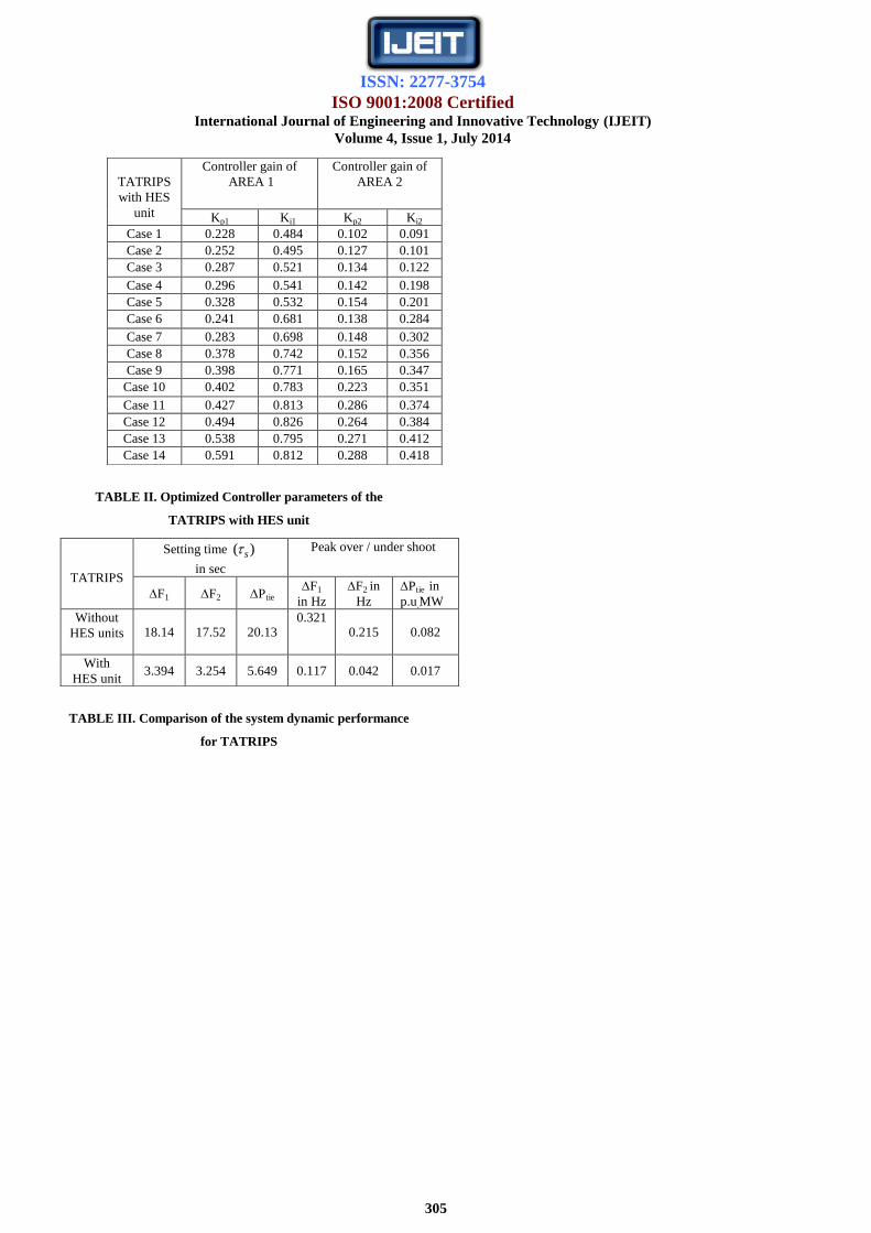
TABLE II. Optimized Controller parameters of the

TATRIPS with HES unit

TABLE III. Comparison of the system dynamic performance

for TATRIPS

TATRIPS

with HES

unit

Controller gain of

AREA 1

Controller gain of

AREA 2

Kp1 Ki1 Kp2 Ki2

Case 1 0.228 0.484 0.102 0.091

Case 2 0.252 0.495 0.127 0.101

Case 3 0.287 0.521 0.134 0.122

Case 4 0.296 0.541 0.142 0.198

Case 5 0.328 0.532 0.154 0.201

Case 6 0.241 0.681 0.138 0.284

Case 7 0.283 0.698 0.148 0.302

Case 8 0.378 0.742 0.152 0.356

Case 9 0.398 0.771 0.165 0.347

Case 10 0.402 0.783 0.223 0.351

Case 11 0.427 0.813 0.286 0.374

Case 12 0.494 0.826 0.264 0.384

Case 13 0.538 0.795 0.271 0.412

Case 14 0.591 0.812 0.288 0.418

TATRIPS

Setting time )( s in sec

Peak over / under shoot

F1 F2 Ptie F1

in Hz

F2 in

Hz

Ptie in

p.u.MW

Without

HES units 18.14 17.52 20.13 0.321

0.215 0.082

With

HES unit 3.394 3.254 5.649 0.117 0.042 0.017

Volume 4, Issue 1, July 2014 Load Frequency Control in a ... 4/Issue 1/IJEIT1412201407_51.pdf ·...

Documents

Transcript of Volume 4, Issue 1, July 2014 Load Frequency Control in a ... 4/Issue 1/IJEIT1412201407_51.pdf ·...