
Volume 3, Issue 4 December 2016 - NSCJ · Volume 3, Issue 4 December 2016 Featured article: A...
52
North Sea Conference & Journal LTD 2 Charlestown Walk, Cove Bay, AB12 3EZ, Aberdeen, Scotland, United Kingdom http://www.nscj.co.uk/JECM/ | [email protected] | +44(0)1224 875635 Volume 3, Issue 4 December 2016 Featured article: A GIS-based statistical approach to prioritize the retrofit of housing stocks at the urban scale Alessio Mastrucci 1* , Olivier Baume 2 , Francesca Stazi 3 , Ulrich Leopold 4 1 International Institute for Applied Systems Analysis, Schlossplatz 1, A-2361 Laxenburg, Austria 2 Resource Centre for Environmental Technologies - Public Research Centre Henri Tudor, 6A, avenue des Hauts-Fourneaux, L-4362 Esch-sur-Alzette, Luxembourg 3 Dipartimento di Ingegneria Civile, Edile e Architettura - Universita Politecnica delle Marche, Via Brecce Bianche 12, 60131 Ancona, Italy 4 Luxembourg Institute of Science and Technology, 5 avenue des Hauts-Fourneaux, L-4362 Esch-sur-Alzette.
Transcript of Volume 3, Issue 4 December 2016 - NSCJ · Volume 3, Issue 4 December 2016 Featured article: A...

North Sea Conference & Journal LTD
2 Charlestown Walk, Cove Bay, AB12 3EZ, Aberdeen, Scotland, United Kingdom http://www.nscj.co.uk/JECM/ | [email protected] | +44(0)1224 875635
Volume 3, Issue 4 December 2016
Featured article:
A GIS-based statistical approach to prioritize the retrofit of housing stocks at the urban scale Alessio Mastrucci1*, Olivier Baume2, Francesca Stazi3, Ulrich Leopold4 1International Institute for Applied Systems Analysis, Schlossplatz 1, A-2361 Laxenburg, Austria 2Resource Centre for Environmental Technologies - Public Research Centre Henri Tudor, 6A, avenue des Hauts-Fourneaux, L-4362 Esch-sur-Alzette, Luxembourg 3Dipartimento di Ingegneria Civile, Edile e Architettura - Universita Politecnica delle Marche, Via Brecce Bianche 12, 60131 Ancona, Italy 4Luxembourg Institute of Science and Technology, 5 avenue des Hauts-Fourneaux, L-4362 Esch-sur-Alzette.
i ©2016
ISSN 2056-9386
Volume 3 (2016) issue 4
TABLE OF CONTENTS pages
Article 1: Wind power plant resonances Luis Sainz1*, Marc Cheah-Mane2*, Lluis Monjo3, Jun Liang2, Oriol Gomis-Bellmunt1 1Department of Electrical Engineering, ETSEIB-UPC, Av. Diagonal 647, Barcelona 08028, Spain 2School of Engineering, Cardiff University, CF24 3AA, Cardiff, U.K 3Department of Industrial and Design System Engineering, ESTCE, Univ. Jaume I, Av. de Vicent Sos Baynat, s/n, 12071 Castelló de la Plana, Spain
168-
179
Article 2: The need for lithium – an upcoming problem for electrochemical energy storages? Daniel Schultz1, Wilhelm Kuckshinrichs1*
1Institute for Energy and Climate Research – Systems Analysis and Technology Evaluation, Forschungszentrum Jülich, 52425 Jülich, Germany
180-
185
Article 3: A GIS-based statistical approach to prioritize the retrofit of housing stocks at the urban scale Alessio Mastrucci1*, Olivier Baume2, Francesca Stazi3, Ulrich Leopold4 1International Institute for Applied Systems Analysis, Schlossplatz 1, A-2361 Laxenburg, Austria 2Resource Centre for Environmental Technologies - Public Research Centre Henri Tudor, 6A, avenue des Hauts-Fourneaux, L-4362 Esch-sur-Alzette, Luxembourg 3Dipartimento di Ingegneria Civile, Edile e Architettura - Universita Politecnica delle Marche, Via Brecce Bianche 12, 60131 Ancona, Italy 4Luxembourg Institute of Science and Technology, 5 avenue des Hauts-Fourneaux, L-4362 Esch-sur-Alzette.
186-
190
Article 4: Parametric modeling of producer gas-combustor and heat exchanger integration for micro-gas turbine application Mackay A.E. Okure1, Wilson B. Musinguzi2*, Terese Løvås3 1School of Engineering, Makerere University, P.O. Box 7062, Kampala, Uganda 2Faculty of Engineering, Busitema University, P.O. Box 236, Tororo, Uganda 3Department of Energy and Process Engineering, NTNU, Trondheim, Norway
191-
200
Article 5: Behavior, cutting property and environmental load of machine tool in mist of strong alkaline water Ikuo Tanabe1* 1Department of Mechanical Engineering, Nagaoka University of Technology, 1603-1 Kamitomioka Nagaoka Niigata, 940-2188 Japan
201-210

ii ©2016
ISSN 2056-9386
Volume 3 (2016) issue 4
Article 6: Korea's policies, R&D investment and competitiveness in the LED industry Joon Han1, Chul-Ho Park1*, Ji-Sun Ku1, Ho-Sik Chon2 1Center for Climate Technology Cooperation, Green Technology Center Korea, Seoul, Korea 2Division of Policy Research, Green Technology Center Korea, Seoul, Korea
211-216

ISSN 2056-9386
Volume 3 (2016) issue 4, article 1
168 ©2016
Wind power plant resonances
风力发电厂的共振
Luis Sainz1*, Marc Cheah-Mane2*, Lluis Monjo3, Jun Liang2, Oriol Gomis-Bellmunt1
1Department of Electrical Engineering, ETSEIB-UPC, Av. Diagonal 647, Barcelona 08028, Spain 2School of Engineering, Cardiff University, CF24 3AA, Cardiff, U.K
3Department of Industrial and Design System Engineering, ESTCE, Univ. Jaume I, Av. de Vicent Sos Baynat, s/n, 12071 Castelló
de la Plana, Spain
Accepted for publication on 30th July 2016
Abstract - Onshore and offshore wind power plants comprising
wind turbines equipped with power converters are increasing in
number worldwide. Harmonic emissions in power converters
distort currents and voltages, leading to power quality problems.
Low order resonances in the collector grid can increase the
impact of wind turbine emissions. These resonances may also
produce electrical instabilities in poorly damped wind power
plants. The paper performs frequency scan with
Matlab/Simulink simulations and compares low order
frequencies of parallel resonances in onshore and offshore wind
power plants. It also investigates the influence of wind power
plant variables on resonance. Finally, simplified equivalent
circuits of wind power plants are proposed to study low order
parallel resonances.
Keywords - Wind power generation, resonance, frequency
scan.
I. INTRODUCTION
The presence of wind power plants (WPPs) with wind
turbines (WTs) equipped with power electronics is currently
increasing in traditional power systems [1]. Several power
quality concerns related to harmonic emissions of these WTs
are present in WPPs [1] [6]. These concerns increase with
parallel resonances in the WPP collector grid at frequencies
close to harmonic emissions. These resonances are due to the
interaction between inductors and capacitors of the WPP
network, [1], [4] [9]. Several works study WPP resonance to
address harmonic concerns [4] [9]. The most important
WPP harmonic and resonance issues are illustrated in [4], [6],
[8]. Recent works also study resonance influence on stability
of WT converters [10] [12]. Low order resonances are the
most worrisome because they can be close to low order
harmonic emissions of power converters and to the poorly
damped frequency range. Resonance studies are mainly based
on frequency scan analysis, which establishes the frequency
range and peak impedance values of resonances. A few works
include analytical expressions to determine low order parallel
resonance frequency [8], [13], [14]. The influence of WPP
parameters on resonances is also discussed in most of the
above studies. In order to investigate this influence further, it
is necessary to examine WPP resonance frequencies in depth
from frequency scan or analytical expressions which
characterize resonance frequencies as a function of WPP
parameters [14].
The present work analyzes WPP parallel resonance from
frequency scan with Matlab/Simulink simulations. It
compares low order parallel resonance frequencies in onshore
and offshore WPPs. The impact of WPP parameters on
resonance is also investigated. Approximated equivalent
circuits for analyzing WPP parallel resonance are proposed
from the above studies.
II. WIND POWER PLANTS
The configuration of a generic WPP layout is shown in
Fig. 1. Type 4 WTs are supplied from the strings of the Nr x Nc
HV/MV
transformers
WT1Nc
WTNrNc
MV
underground/submarine
cable
(onshore/offshore WPPs)
WT11
WTNr1
Nr Nc
MV/LV
transformer
MV collector
bus
High frequency
filter
Main grid
HV submarine cable
(offshore WPPs)
Capacitor
bank
Fig.1. Wind power plant layout

Sainz et al. (2016) Wind power plant resonances
169 Journal of Energy Challenges and Mechanics ©2016
collector grid through step-down medium to low voltage
(MV/LV) transformers. High frequency filter capacitors are
usually installed on the grid-side of WT converters to mitigate
frequency switching harmonics [4], [5]. The strings are
interconnected with medium voltage (MV) underground
cables in onshore WPPs and MV submarine cables in offshore
WPPs. These cables are clustered at the MV collector bus [4],
[5], [6] [10], [13]. In onshore WPPs, capacitor banks can
also be connected to this bus in order to compensate reactive
power. The MV collector bus is connected to the main grid
with two step-down high to medium voltage (HV/MV)
transformers in parallel. In onshore WPPs, the transformers
are directly connected to the main grid while, in offshore
WPPs, high voltage (HV) submarine cables are used to link
the transformers to the main grid on shore.
Voltage distortion of the WPP collector grid usually
remains below standard limits because WT converter
harmonic emissions are generally low [2], [3], [15], [16].
However, parallel resonances may increase distortion above
these limits and affect WT operation if the resonance
frequency is close to WT converter emission harmonics [4],
[5]. These resonances may also affect stability of WT
converters [10] [12]. The frequency scan method is
commonly used in the literature to characterize the resonance
problem at WT terminals and approach harmonic penetration
and WT stability studies.
II. WIND POWER PLANT HARMONIC MODEL
In order to perform frequency scan, the WPPs are
characterized by the equivalent circuit in Fig. 2, and the
equivalent harmonic impedance ZEq, k at the WTs must be
determined to identify resonance frequencies. To do that, the
harmonic impedances of the main grid, ZS, k, HV/MV and
MV/LV transformers, ZT, k, HV and MV
underground/submarine cables, ZL, k, capacitor bank, ZCb, k, and
high frequency filters, ZCf, k, are modeled as follows [4], [5],
[7]:
2
,2
2
,s
,2
, ,
, ,, ,
, ,
2
, ,
1
11 tan
1 tan
11 tan
1 tan
sinh tanh 2
2
1 1,
OS k S
S S
N
T k cc cc
N cc
x k x k
C k Cx kL k Lx k
x k x k
NbCb k Cf k
Cb f
UZ jk
S
UZ jk
S
D DZ Z Y Y
UZ j Z j
k Q C k
(1)
where k = fk/f1 (with fk and f1 being the analyzed harmonic
frequency and the main grid fundamental frequency,
respectively), 1 = 2·f1 and,
UO, SS and tanS are the main grid open-circuit voltage,
ZT, k/2
WT11
Nr Nc
WTNrNc
ZS, k
ZT, k
WT1Nc
ZEq, k
HV submarine cable
(offshore WPPs)
HV/MV
transformers
MV
underground/submarine
cable
(onshore/offshore WPPs)
Main grid
MV/LV
transformer
MV collector
bus
ZL, k
YC, k/2
YC, k/2
ZL, k
YC, k/2
YC, k/2
IWT, k ZCf, k
WTNr1
High frequency
filter
ZCb, k
Capacitor
bank
Fig.2. Wind power plant equivalent circuit
TABLE 1. WPP PARAMETERS (WTS OF PWT = 5 MW)
Main grid
U0 (f1) 150 kV (50 Hz)
SS (10…100)·NrNcPWT
tanS 20 pu
HV/MV
transformers
UN, H/UN, M 150/33 kV
SN 125 MVA
cc (tancc) 0.1 pu (12 pu)
MV/LV
transformer
UN, M/UN, L 33/0.69 kV
SN 5 MVA
cc (tancc) 0.05 pu (12 pu)
HV submarine
cable
(offshore WPPs)
Rx 0.032 /km
Lx 0.401 mH/km
Cx 0.21 F/km
DHV 1 to 50 km
MV underground
/submarine cable
(onshore/offshore
WPPs)
Rx 0.041 /km
Lx 0.38 mH/km
Cx 0.23 F/km
DMV 0.5 to 1 km
Compensation
and filter
equipment
QCb 0 … 50 Mvar
Cf 1000 F

Sainz et al. (2016) Wind power plant resonances
170 Journal of Energy Challenges and Mechanics ©2016
short-circuit power and XS/RS ratio at the point of
coupling.
UN, p /UN, s, SN, cc and tancc are the HV/MV and MV/LV
transformer rated primary/secondary voltages and power,
per-unit short-circuit impedance and Xcc/Rcc ratio.
x, k = (ZLx, k·YCx, k)1/2 is the propagation constant of the
cable, ZLx, k = Rx + jLxk1 and YLx, k = jCxk1 are the cable
distributed parameters and D is the cable length.
UNb and QCb are the capacitor bank rated voltage and
reactive power consumption (i.e., the capacitor bank
size).
Cf is the WT high frequency filter capacitor.
The transformers are modeled as RL equivalent circuits and
the WTs are modeled as ideal current sources. These models
are accurate enough to analyze the influence of WPP
parameters on low order resonances. The WT current source
model is commonly chosen to perform frequency scan studies
because it offers a useful insight into low order parallel
resonance analysis [1], [4], [5] [8], [13]. Table 1 shows usual
WPP parameter values.
II. ONSHORE AND OFFSHORE WPP RESONANCES
The frequency response of an 8x5 onshore and an 8x5
offshore WPP (data in Table 1) is determined to compare their
low order parallel resonances. Both WPPs consist of 40 type 4
WTs (i.e., full-scale VSC WTs), each with a rated capacity of
5 MW, arranged in five strings of 33 kV
underground/submarine cables. These strings collect eight
WTs (separated 1 km from each other) at the collector
substation. This substation is directly connected to the main
grid in the onshore WPP and by a 25 km submarine cable in
the offshore WPP. The short circuit power of the main grid is
2500 MVA and capacitor banks are not connected to the
collector bus of the onshore WPP (i.e., QCb = 0 Mvar). The
results of the equivalent harmonic impedance ZEq, k at WTNr1
(see Fig. 2) are illustrated in Fig. 3. From these results, it can
be noted that
WPP connection to shore by the HV submarine cable is
the only difference between the onshore and offshore
WPPs. The difference between the first parallel
resonances of the onshore WPP (at f1on = 592 Hz) and
offshore WPP (at f1off = 336 Hz) is due to the transversal
capacitors of the cable. These capacitors shift the parallel
resonance to low order frequencies, which are close to
WT harmonic emissions.
The HV submarine cable of the offshore WPP also
produces a parallel resonance at f2off = 902 Hz which does
not appear in the onshore WPP. The frequency of this
parallel resonance depends on the cable length, as is
analyzed in Subsection 4.3.
Parallel resonances above 1 kHz (i.e., f3off f2on and
f4off f3on) are not affected by the capacitors of the HV
submarine cable, thus being similar in both WPPs.
III. ONSHORE WPP RESONANCE STUDY
The frequency response of the 8x5 onshore WPP in
Section II (data in Table 1) is analyzed to study the influence
of the main grid short circuit ratio, SCR = SS/(Nr·Nc·PWT),
WPP layout (i.e., number of WTs and strings Nr, and Nc), MV
underground cable length, DMV, and capacitor bank size, QCb,
on low order parallel resonances. To study the influence of
these parameters, Matlab/Simulink simulations are made by
varying their values. In these simulations, frequency scan is
ZW
T (
)
0.001
100
1
10
0.01
0.1
f (kHz)
f1off = 336 Hz f3off f2on = 1109 Hz
0 0.8 1.2 0.4 1.6 2.0
f2off = 902 Hz
f1on = 592 Hz
f4off f3on = 1290 Hz
Fig. 3. Frequency scan of 8x5 onshore (black line) and offshore (red
line) WPPs (data in Table 1, with SS = 2500 MVA, DHV = 25 km,
DMV = 1 km and QCb = 0 Mvar)
ZW
T (
)
0.001
100
1
10
0.01
0.1
f (kHz)
0 0.8 1.2 0.4 1.6 2.0
749 Hz 592 Hz
f 1on (
kH
z)
0.55
0.9
0.65
0.7
0.6
SCR = SS/(Nr·Nc·PWT) (pu) 10 50 100
a)
b)
0.75
788 Hz
20 30 40 60 70 80 90
0.8
0.85
12.5
50
100
SCR (pu)
Fig. 4. Influence of the short circuit ratio, SCR, of the main grid on
8x5 onshore WPP resonance (data in Table 1, with DMV = 1 km and
QCb = 0 Mvar): a) Frequency scan. b) Frequency of first parallel
resonance vs Short circuit ratio (black lines: Equivalent circuit in
Fig. 2; red lines: Equivalent circuit in Fig. 19)
Sainz et al. (2016) Wind power plant resonances
171 Journal of Energy Challenges and Mechanics ©2016
performed at WTNr1 (see Fig. 2) and the equivalent harmonic
impedance ZEq, k is obtained. Subsequently, the frequency of
the parallel resonances is numerically identified from the
frequency scan.
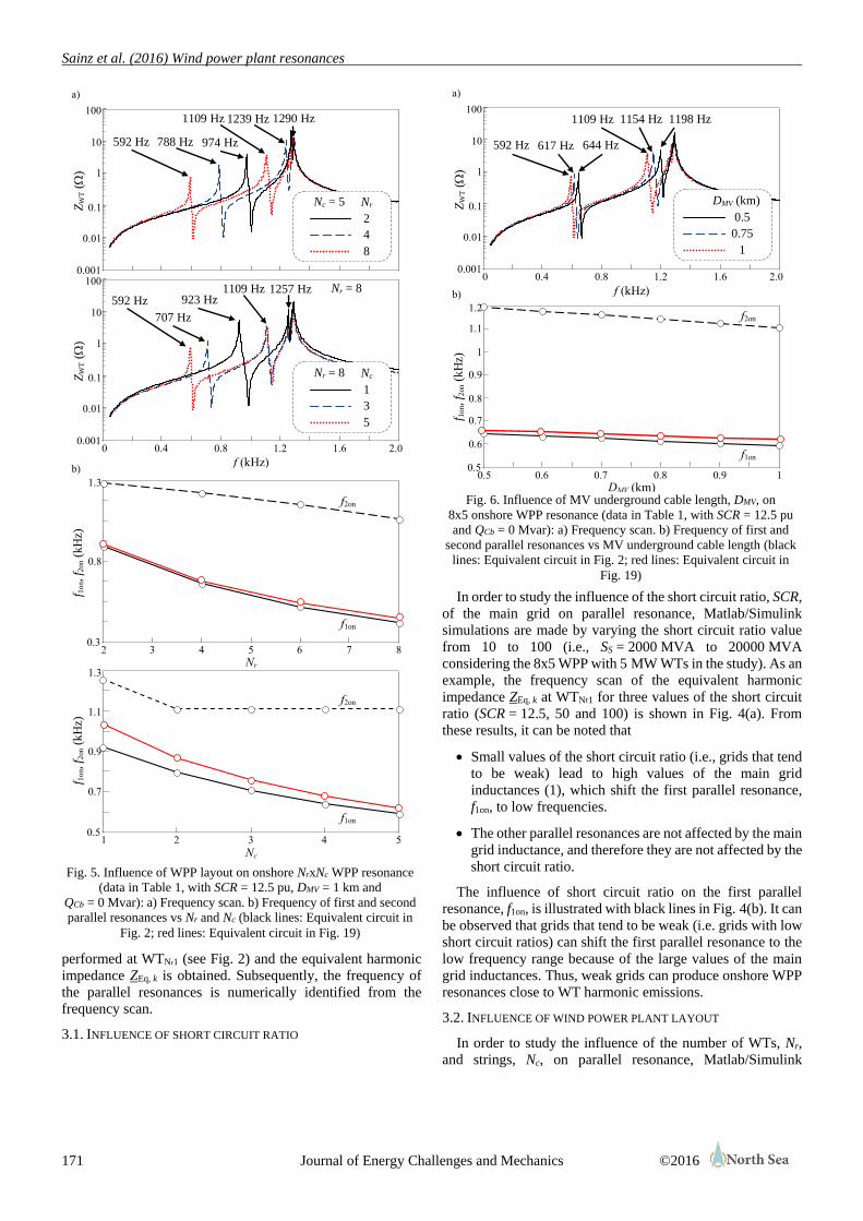
3.1. INFLUENCE OF SHORT CIRCUIT RATIO
In order to study the influence of the short circuit ratio, SCR,
of the main grid on parallel resonance, Matlab/Simulink
simulations are made by varying the short circuit ratio value
from 10 to 100 (i.e., SS = 2000 MVA to 20000 MVA
considering the 8x5 WPP with 5 MW WTs in the study). As an
example, the frequency scan of the equivalent harmonic
impedance ZEq, k at WTNr1 for three values of the short circuit
ratio (SCR = 12.5, 50 and 100) is shown in Fig. 4(a). From
these results, it can be noted that
Small values of the short circuit ratio (i.e., grids that tend
to be weak) lead to high values of the main grid
inductances (1), which shift the first parallel resonance,
f1on, to low frequencies.
The other parallel resonances are not affected by the main
grid inductance, and therefore they are not affected by the
short circuit ratio.
The influence of short circuit ratio on the first parallel
resonance, f1on, is illustrated with black lines in Fig. 4(b). It can
be observed that grids that tend to be weak (i.e. grids with low
short circuit ratios) can shift the first parallel resonance to the
low frequency range because of the large values of the main
grid inductances. Thus, weak grids can produce onshore WPP
resonances close to WT harmonic emissions.
3.2. INFLUENCE OF WIND POWER PLANT LAYOUT
In order to study the influence of the number of WTs, Nr,
and strings, Nc, on parallel resonance, Matlab/Simulink
f 1o
n, f 2
on (
kH
z)
0.3
1.3
0.8
Nr 2 8
a)
b)
3 4 5 6 7
ZW
T (
)
0.001
100
1
10
0.01
0.1
592 Hz
1109 Hz
788 Hz
1239 Hz
974 Hz
1290 Hz
ZW
T (
)
0.001
100
1
10
0.01
0.1
f (kHz)
592 Hz
0 0.8 1.2 0.4 1.6 2.0
1109 Hz
707 Hz
923 Hz 1257 Hz
0.5
1.3
0.9
Nc 1 5 2 3 4
Nr = 8
0.7
1.1
f2on
f1on
f2on
f1on
f 1o
n, f 2
on (
kH
z)
Nc = 5
2
4
8
Nr
Nr = 8
1
3
5
Nc
Fig. 5. Influence of WPP layout on onshore NrxNc WPP resonance
(data in Table 1, with SCR = 12.5 pu, DMV = 1 km and
QCb = 0 Mvar): a) Frequency scan. b) Frequency of first and second
parallel resonances vs Nr and Nc (black lines: Equivalent circuit in
Fig. 2; red lines: Equivalent circuit in Fig. 19)
ZW
T (
)
0.001
100
1
10
0.01
0.1
f (kHz)
1109 Hz
0 0.8 1.2 0.4 1.6 2.0
617 Hz 592 Hz
0.5
1.2
0.7
0.8
0.6
DMV (km) 0.5 0.7 1
a)
b)
1
644 Hz
0.6 0.8 0.9
1154 Hz 1198 Hz
1.1
0.9
f 1o
n, f 2
on (
kH
z)
f2on
f1on
0.5
0.75
1
DMV (km)
Fig. 6. Influence of MV underground cable length, DMV, on
8x5 onshore WPP resonance (data in Table 1, with SCR = 12.5 pu
and QCb = 0 Mvar): a) Frequency scan. b) Frequency of first and
second parallel resonances vs MV underground cable length (black
lines: Equivalent circuit in Fig. 2; red lines: Equivalent circuit in
Fig. 19)
Sainz et al. (2016) Wind power plant resonances
172 Journal of Energy Challenges and Mechanics ©2016
simulations are made by varying the Nr value from 2 to 8 and
the Nc value from 1 to 5. As an example, the frequency scan of
the equivalent harmonic impedance ZEq, k at WTNr1 for three
values of Nr (Nr = 2, 4 and 8) and for three values of Nc
(Nc = 1, 3 and 5) is shown in Fig. 5(a). From these results, it
can be noted that
High number of the WTs and strings shift the first and
second parallel resonances, f1on and f2on, to low
frequencies.
The influence of WPP layout on the first and second parallel
resonances f1on and f2on is illustrated with black lines in
Fig. 5(b). It can be observed that parallel resonances are closer
to low order harmonics in large onshore WPPs than in small
onshore WPPs because parallel resonance frequencies move to
lower order harmonics with increasing the number of WTs and
strings. An exhaustive study of this influence is presented in
[14].
3.3. INFLUENCE OF MV UNDERGROUND CABLE LENGTH
In order to study the influence of MV underground cable
length, DMV, on parallel resonance, Matlab/Simulink
simulations are made by varying the cable length value from
0.5 km to 1 km. As an example, the frequency scan of the
equivalent harmonic impedance ZEq, k at WTNr1 for three values
of the cable length (DMV = 0.5, 0.75 and 1 km) is shown in
Fig. 6(a). From these results, it can be noted that
High values of the MV cable length shift the first and
second parallel resonances, f1on and f2on, to low
frequencies because of the higher value of transversal
capacitors of the cable. However, these resonance
frequencies exhibit a low sensitivity to MV cable length.
The other parallel resonance is not affected by cable
length.
The influence of MV cable length on the first and second
parallel resonances f1on and f2on is illustrated with black lines in
Fig. 6(b). It can be observed that, although the frequency of
the parallel resonances is only slightly affected by cable
length, it decreases with long MV underground cables. Thus,
WPPs with WTs far away from each other can produce
onshore WPP resonances close to WT harmonic emissions.
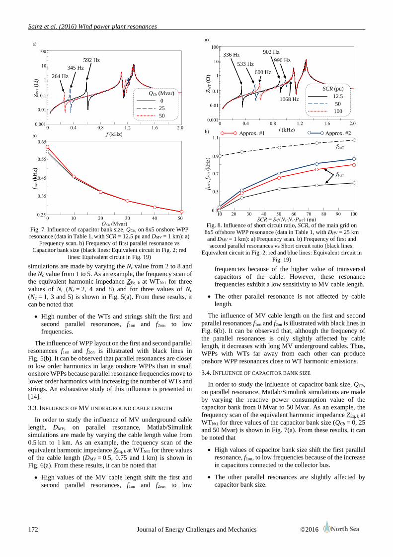
3.4. INFLUENCE OF CAPACITOR BANK SIZE
In order to study the influence of capacitor bank size, QCb,
on parallel resonance, Matlab/Simulink simulations are made
by varying the reactive power consumption value of the
capacitor bank from 0 Mvar to 50 Mvar. As an example, the
frequency scan of the equivalent harmonic impedance ZEq, k at
WTNr1 for three values of the capacitor bank size (QCb = 0, 25
and 50 Mvar) is shown in Fig. 7(a). From these results, it can
be noted that
High values of capacitor bank size shift the first parallel
resonance, f1on, to low frequencies because of the increase
in capacitors connected to the collector bus.
The other parallel resonances are slightly affected by
capacitor bank size.
0.3
1.1
0.7
0.5
10 50 100
a)
b)
0.9
20 30 40 60 70 80 90 Z
WT (
)
0.001
100
1
10
0.01
0.1
f (kHz)
336 Hz
0 0.8 1.2 0.4 1.6 2.0
902 Hz
533 Hz 990 Hz
600 Hz
1068 Hz
Approx. #1 Approx. #2
f 1o
ff, f 2
off (
kH
z)
f2off
f1off
SCR = SS/(Nr·Nc·PWT) (pu)
12.5
50
100
SCR (pu)
Fig. 8. Influence of short circuit ratio, SCR, of the main grid on
8x5 offshore WPP resonance (data in Table 1, with DHV = 25 km
and DMV = 1 km): a) Frequency scan. b) Frequency of first and
second parallel resonances vs Short circuit ratio (black lines:
Equivalent circuit in Fig. 2; red and blue lines: Equivalent circuit in
Fig. 19)
ZW
T (
)
0.001
100
1
10
0.01
0.1
f (kHz)
0 0.8 1.2 0.4 1.6 2.0
592 Hz
345 Hz
264 Hz
f 1on (
kH
z)
0.25
0.65
0.45
0.35
QCb (Mvar) 0 20 30 10 40 50
a)
b)
0.55
0
25
50
QCb (Mvar)
Fig. 7. Influence of capacitor bank size, QCb, on 8x5 onshore WPP
resonance (data in Table 1, with SCR = 12.5 pu and DMV = 1 km): a)
Frequency scan. b) Frequency of first parallel resonance vs
Capacitor bank size (black lines: Equivalent circuit in Fig. 2; red
lines: Equivalent circuit in Fig. 19)

Sainz et al. (2016) Wind power plant resonances
173 Journal of Energy Challenges and Mechanics ©2016
The influence of capacitor bank size on the first parallel
resonance, f1on, is illustrated with black lines in Fig. 7(b). It can
be observed that larger capacitor bank sizes lead to lower
frequency values of the first parallel resonance. Thus, reactive
power compensation at the collector bus can produce onshore
WPP resonances close to WT harmonic emissions. An
exhaustive study of capacitor size influence is presented in
[14].
IV. OFFSHORE WPP RESONANCE STUDY
The frequency response of the 8x5 offshore WPP in
Section II (data in Table 1) is analyzed to study the influence
of the main grid short circuit ratio, SCR = SS/(Nr·Nc·PWT),
WPP layout (i.e., number of WTs and strings, Nr and Nc), HV
submarine cable length, DHV, and MV submarine cable length,
DMV, on low order parallel resonances. To do this,
Matlab/Simulink simulations are made by varying their
values. A frequency scan at WTNr1 (see Fig. 2) is performed in
these simulations and the equivalent harmonic impedance
ZEq, k is obtained. Subsequently, the frequency of the parallel
resonance is numerically identified from the frequency scan.
4.1. INFLUENCE OF SHORT CIRCUIT RATIO
In order to study the influence of short circuit ratio, SCR, of
the main grid on parallel resonance, Matlab/Simulink
simulations are made by varying the short circuit ratio value
from 10 to 100 (i.e., SS = 2000 MVA to 20000 MVA
considering the 8x5 WPP with 5 MW WTs in the study). As
an example, the frequency scan of the equivalent harmonic
impedance ZEq, k at WTNr1 for three values of the short circuit
ratio (SCR = 12.5, 50 and 100 pu) is shown in Fig. 8(a). From
these results, it can be noted that
0.3
1.3
0.8
Nr 2 8
a)
b)
3 4 5 6 7
ZW
T (
)
0.001
100
1
10
0.01
0.1
336 Hz 902 Hz
360 Hz
1056 Hz
378 Hz
1162 Hz 1276 Hz
1239 Hz
1109 Hz
ZW
T (
)
0.001
100
1
10
0.01
0.1
f (kHz)
336 Hz
0 0.8 1.2 0.4 1.6 2.0
902 Hz
355 Hz 961 Hz
376 Hz
1049 Hz
0.3
1.1
0.7
Nc 1 5 2 3 4
0.5
0.9
Approx. #1 Approx. #2
f 1o
ff, f 2
off, f 3
off
(kH
z)
f2off
f1off
f2off
f1off
f 1o
ff, f 2
off (
kH
z)
f3off
Nc = 5
2
4
8
Nr
Nr = 8
1
3
5
Nc
Fig. 9. Influence of WPP layout on NrxNc offshore WPP resonance
(data in Table 1, SCR = 12.5 pu, DHV = 25 km and DMV = 1 km): a)
Frequency scan. b) Frequencies of first, second and third parallel
resonances vs Nr and Nc (black lines: Equivalent circuit in Fig. 2;
red and blue lines: Equivalent circuit in Fig. 19)
0.2
1.2
0.4
DHV (km) 0 20 50
a)
b)
0.6
10 30 40
ZW
T (
)
0.001
100
1
10
0.01
0.1
f (kHz)
336 Hz
1109 Hz
0 0.8 1.2 0.4 1.6 2.0
902 Hz
578 Hz
785 Hz 240 Hz
0.8
1
Approx. #1 Approx. #2
f 1o
ff, f 2
off (
kH
z)
f2off
f1off
1
25
50
DHV (km)
Fig. 10. Influence of HV submarine cable length DHV on
8x5 offshore WPP resonance (data in Table 1, with SCR = 12.5 pu
and DMV = 1 km): a) Frequency scan. b) Frequency of first and
second parallel resonances vs MV submarine cable length (black
lines: Equivalent circuit in Fig. 2; red and blue lines: Equivalent
circuit in Fig. 19)
Sainz et al. (2016) Wind power plant resonances
174 Journal of Energy Challenges and Mechanics ©2016
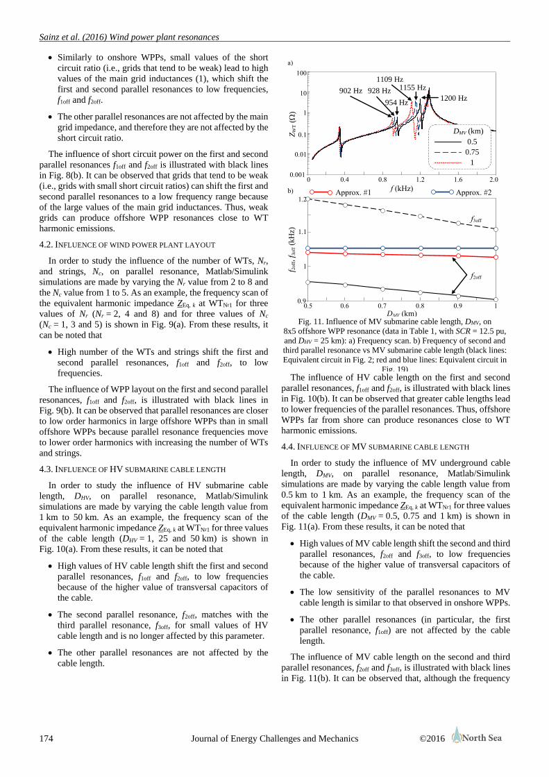
Similarly to onshore WPPs, small values of the short
circuit ratio (i.e., grids that tend to be weak) lead to high
values of the main grid inductances (1), which shift the
first and second parallel resonances to low frequencies,
f1off and f2off.
The other parallel resonances are not affected by the main
grid impedance, and therefore they are not affected by the
short circuit ratio.
The influence of short circuit power on the first and second
parallel resonances f1off and f2off is illustrated with black lines
in Fig. 8(b). It can be observed that grids that tend to be weak
(i.e., grids with small short circuit ratios) can shift the first and
second parallel resonances to a low frequency range because
of the large values of the main grid inductances. Thus, weak
grids can produce offshore WPP resonances close to WT
harmonic emissions.
4.2. INFLUENCE OF WIND POWER PLANT LAYOUT
In order to study the influence of the number of WTs, Nr,
and strings, Nc, on parallel resonance, Matlab/Simulink
simulations are made by varying the Nr value from 2 to 8 and
the Nc value from 1 to 5. As an example, the frequency scan of
the equivalent harmonic impedance ZEq, k at WTNr1 for three
values of Nr (Nr = 2, 4 and 8) and for three values of Nc
(Nc = 1, 3 and 5) is shown in Fig. 9(a). From these results, it
can be noted that
High number of the WTs and strings shift the first and
second parallel resonances, f1off and f2off, to low
frequencies.
The influence of WPP layout on the first and second parallel
resonances, f1off and f2off, is illustrated with black lines in
Fig. 9(b). It can be observed that parallel resonances are closer
to low order harmonics in large offshore WPPs than in small
offshore WPPs because parallel resonance frequencies move
to lower order harmonics with increasing the number of WTs
and strings.
4.3. INFLUENCE OF HV SUBMARINE CABLE LENGTH
In order to study the influence of HV submarine cable
length, DHV, on parallel resonance, Matlab/Simulink
simulations are made by varying the cable length value from
1 km to 50 km. As an example, the frequency scan of the
equivalent harmonic impedance ZEq, k at WTNr1 for three values
of the cable length (DHV = 1, 25 and 50 km) is shown in
Fig. 10(a). From these results, it can be noted that
High values of HV cable length shift the first and second
parallel resonances, f1off and f2off, to low frequencies
because of the higher value of transversal capacitors of
the cable.
The second parallel resonance, f2off, matches with the
third parallel resonance, f3off, for small values of HV
cable length and is no longer affected by this parameter.
The other parallel resonances are not affected by the
cable length.
The influence of HV cable length on the first and second
parallel resonances, f1off and f2off, is illustrated with black lines
in Fig. 10(b). It can be observed that greater cable lengths lead
to lower frequencies of the parallel resonances. Thus, offshore
WPPs far from shore can produce resonances close to WT
harmonic emissions.
4.4. INFLUENCE OF MV SUBMARINE CABLE LENGTH
In order to study the influence of MV underground cable
length, DMV, on parallel resonance, Matlab/Simulink
simulations are made by varying the cable length value from
0.5 km to 1 km. As an example, the frequency scan of the
equivalent harmonic impedance ZEq, k at WTNr1 for three values
of the cable length (DMV = 0.5, 0.75 and 1 km) is shown in
Fig. 11(a). From these results, it can be noted that
High values of MV cable length shift the second and third
parallel resonances, f2off and f3off, to low frequencies
because of the higher value of transversal capacitors of
the cable.
The low sensitivity of the parallel resonances to MV
cable length is similar to that observed in onshore WPPs.
The other parallel resonances (in particular, the first
parallel resonance, f1off) are not affected by the cable
length.
The influence of MV cable length on the second and third
parallel resonances, f2off and f3off, is illustrated with black lines
in Fig. 11(b). It can be observed that, although the frequency
0.9
1.2
1
DMV (km) 0.5 0.7 1
a)
b)
1.1
0.6 0.8 0.9
ZW
T (
)
0.001
100
1
10
0.01
0.1
f (kHz)
1109 Hz
0 0.8 1.2 0.4 1.6 2.0
902 Hz 928 Hz 1155 Hz
954 Hz 1200 Hz
Approx. #1 Approx. #2
f 2off, f 3
off (
kH
z)
f3off
f2off
0.5
0.75
1
DMV (km)
Fig. 11. Influence of MV submarine cable length, DMV, on
8x5 offshore WPP resonance (data in Table 1, with SCR = 12.5 pu,
and DHV = 25 km): a) Frequency scan. b) Frequency of second and
third parallel resonance vs MV submarine cable length (black lines:
Equivalent circuit in Fig. 2; red and blue lines: Equivalent circuit in
Fig. 19)
Sainz et al. (2016) Wind power plant resonances
175 Journal of Energy Challenges and Mechanics ©2016
of the parallel resonances is only slightly affected by cable
length, it decreases with long MV submarine cables. Thus,
WPPs with WTs far away from each other can produce
resonances close to WT harmonic emissions.
V. INFLUENCE OF WPP ELECTRICAL PARAMETERS
In order to study the influence of WPP electrical parameters
on parallel resonance, the frequency scan of the equivalent
harmonic impedance ZEq, k at WTNr1 with the parameter values
in Table 1 and with the parameter values increased by 20% is
compared for onshore and offshore WPPs.
5.1. ONSHORE WIND POWER PLANTS
The influence of the following electrical parameters is
analyzed:
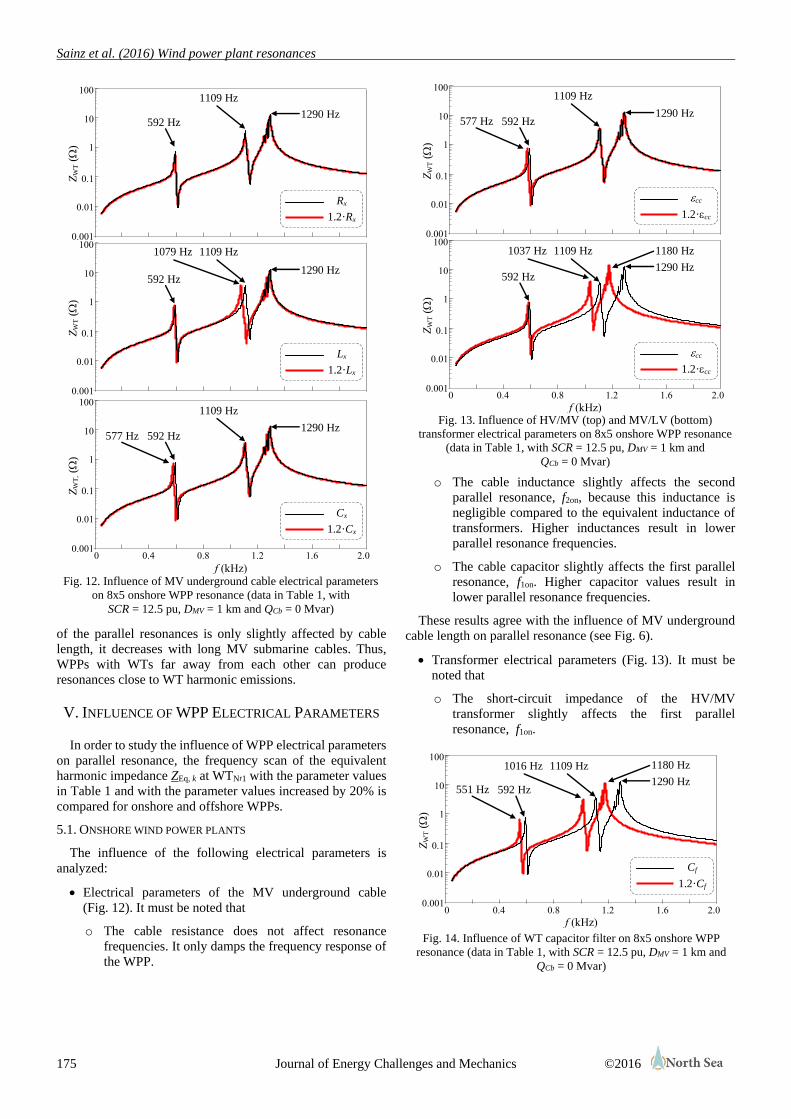
Electrical parameters of the MV underground cable
(Fig. 12). It must be noted that
o The cable resistance does not affect resonance
frequencies. It only damps the frequency response of
the WPP.
o The cable inductance slightly affects the second
parallel resonance, f2on, because this inductance is
negligible compared to the equivalent inductance of
transformers. Higher inductances result in lower
parallel resonance frequencies.
o The cable capacitor slightly affects the first parallel
resonance, f1on. Higher capacitor values result in
lower parallel resonance frequencies.
These results agree with the influence of MV underground
cable length on parallel resonance (see Fig. 6).
Transformer electrical parameters (Fig. 13). It must be
noted that
o The short-circuit impedance of the HV/MV
transformer slightly affects the first parallel
resonance, f1on.
f (kHz) 0 0.8 1.2 0.4 1.6 2.0
ZW
T (
)
0.001
100
1
10
0.01
0.1
1109 Hz
592 Hz
1016 Hz
551 Hz
Cf
1.2·Cf
1290 Hz
1180 Hz
Fig. 14. Influence of WT capacitor filter on 8x5 onshore WPP
resonance (data in Table 1, with SCR = 12.5 pu, DMV = 1 km and
QCb = 0 Mvar)
f (kHz) 0 0.8 1.2 0.4 1.6 2.0
ZW
T (
)
0.001
100
1
10
0.01
0.1
1109 Hz
ZW
T (
)
0.001
100
1
10
0.01
0.1
1037 Hz
cc
1.2·cc
cc
1.2·cc
1290 Hz
1290 Hz
1180 Hz
1109 Hz
592 Hz 577 Hz
592 Hz
Fig. 13. Influence of HV/MV (top) and MV/LV (bottom)
transformer electrical parameters on 8x5 onshore WPP resonance
(data in Table 1, with SCR = 12.5 pu, DMV = 1 km and
QCb = 0 Mvar)
ZW
T, (
)
0.001
100
1
10
0.01
0.1
f (kHz)
0 0.8 1.2 0.4 1.6 2.0
ZW
T (
)
0.001
100
1
10
0.01
0.1
ZW
T (
)
0.001
100
1
10
0.01
0.1
Rx
1.2·Rx
Lx
1.2·Lx
Cx
1.2·Cx
1290 Hz
1290 Hz
1290 Hz
1109 Hz 1079 Hz
1109 Hz
1109 Hz
592 Hz
592 Hz
592 Hz 577 Hz
Fig. 12. Influence of MV underground cable electrical parameters
on 8x5 onshore WPP resonance (data in Table 1, with
SCR = 12.5 pu, DMV = 1 km and QCb = 0 Mvar)
Sainz et al. (2016) Wind power plant resonances
176 Journal of Energy Challenges and Mechanics ©2016
o The short-circuit impedance of the MV/LV
transformer significantly affects the second parallel
resonance, f2on.
WT filter capacitor (Fig. 14). The presence of this
capacitor must be considered in onshore WPP resonance
studies because it significantly affects all the parallel
resonances.
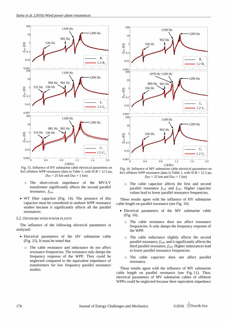
5.2. OFFSHORE WIND POWER PLANTS
The influence of the following electrical parameters is
analyzed:
Electrical parameters of the HV submarine cable
(Fig. 15). It must be noted that
o The cable resistance and inductance do not affect
resonance frequencies. The resistance only damps the
frequency response of the WPP. They could be
neglected compared to the equivalent impedance of
transformers for low frequency parallel resonance
studies.
o The cable capacitor affects the first and second
parallel resonance f1off and f2off. Higher capacitor
values lead to lower parallel resonance frequencies.
These results agree with the influence of HV submarine
cable length on parallel resonance (see Fig. 10).
Electrical parameters of the MV submarine cable
(Fig. 16).
o The cable resistance does not affect resonance
frequencies. It only damps the frequency response of
the WPP.
o The cable inductance slightly affects the second
parallel resonance, f2off, and it significantly affects the
third parallel resonance, f3off. Higher inductances lead
to lower parallel resonance frequencies.
o The cable capacitor does not affect parallel
resonance.
These results agree with the influence of MV submarine
cable length on parallel resonance (see Fig. 11). Thus,
electrical parameters of MV submarine cables of offshore
WPPs could be neglected because their equivalent impedance
Z
WT (
)
0.001
100
1
10
0.01
0.1
f (kHz)
0 0.8 1.2 0.4 1.6 2.0
ZW
T (
)
0.001
100
1
10
0.01
0.1
ZW
T (
)
0.001
100
1
10
0.01
0.1
336 Hz
902 Hz
332 Hz
894 Hz
336 Hz
902 Hz
314 Hz
881 Hz
1109 Hz
1109 Hz
1109 Hz
336 Hz
902 Hz
1290 Hz
1290 Hz
1290 Hz
Rx
1.2·Rx
Lx
1.2·Lx
Cx
1.2·Cx
Fig. 15. Influence of HV submarine cable electrical parameters on
8x5 offshore WPP resonance (data in Table 1, with SCR = 12.5 pu,
DHV = 25 km and DMV = 1 km)
ZW
T (
)
0.001
100
1
10
0.01
0.1
f (kHz)
0 0.8 1.2 0.4 1.6 2.0
ZW
T (
)
0.001
100
1
10
0.01
0.1
ZW
T (
)
0.001
100
1
10
0.01
0.1
1109 Hz
336 Hz
902 Hz
1109 Hz
336 Hz
902 Hz
1078 Hz
1109 Hz
336 Hz
902 Hz
1290 Hz
1290 Hz
1290 Hz
Rx
1.2·Rx
Lx
1.2·Lx
Cx
1.2·Cx
889 Hz
Fig. 16. Influence of MV submarine cable electrical parameters on
8x5 offshore WPP resonance (data in Table 1, with SCR = 12.5 pu,
DHV = 25 km and DMV = 1 km)
Sainz et al. (2016) Wind power plant resonances
177 Journal of Energy Challenges and Mechanics ©2016
is small and only affects the high frequency parallel
resonances.
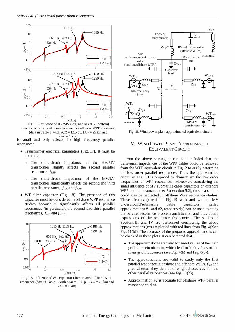
Transformer electrical parameters (Fig. 17). It must be
noted that
o The short-circuit impedance of the HV/MV
transformer slightly affects the second parallel
resonance, f2off.
o The short-circuit impedance of the MV/LV
transformer significantly affects the second and third
parallel resonance, f2off and f3off.
WT filter capacitor (Fig. 18). The presence of this
capacitor must be considered in offshore WPP resonance
studies because it significantly affects all parallel
resonances (in particular, the second and third parallel
resonances, f2off and f3off).
VI. WIND POWER PLANT APPROXIMATED
EQUIVALENT CIRCUIT
From the above studies, it can be concluded that the
transversal impedances of the WPP cables could be removed
from the WPP equivalent circuit in Fig. 2 to easily determine
the low order parallel resonances. Thus, the approximated
circuit of Fig. 19 is proposed to characterize the low order
frequencies of WPP resonances. Moreover, considering the
small influence of MV submarine cable capacitors on offshore
WPP parallel resonance (see Subsection 5.2), these capacitors
could also be neglected in offshore WPP resonance studies.
These circuits (circuit in Fig. 19 with and without MV
underground/submarine cable capacitors, called
approximations #1 and #2, respectively) can be used to study
the parallel resonance problem analytically, and thus obtain
expressions of the resonance frequencies. The studies in
Sections III and IV are performed considering the above
approximations (results plotted with red lines from Fig. 4(b) to
Fig. 11(b)). The accuracy of the proposed approximations can
be checked in these plots. It can be noted that,
The approximations are valid for small values of the main
grid short circuit ratio, which lead to high values of the
main grid inductances (see Fig. 4(b) and Fig. 8(b)).
The approximations are valid to study only the first
parallel resonance in onshore and offshore WPPs, f1on and
f1off, whereas they do not offer good accuracy for the
other parallel resonances (see Fig. 11(b)).
Approximation #2 is accurate for offshore WPP parallel
resonance studies.
f (kHz) 0 0.8 1.2 0.4 1.6 2.0
ZW
T (
)
0.001
100
1
10
0.01
0.1
Cf
1.2·Cf
336 Hz
852 Hz
1290 Hz
902 Hz
1109 Hz 1015 Hz 1180 Hz
330 Hz
Fig. 18. Influence of WT capacitor filter on 8x5 offshore WPP
resonance (data in Table 1, with SCR = 12.5 pu, DHV = 25 km and
DMV = 1 km)
f (kHz) 0 0.8 1.2 0.4 1.6 2.0
ZW
T (
)
0.001
100
1
10
0.01
0.1
ZW
T (
)
0.001
100
1
10
0.01
0.1
336 Hz
902 Hz 869 Hz
875 Hz
336 Hz
1290 Hz
902 Hz
1109 Hz 1037 Hz
1109 Hz
1180 Hz
1290 Hz
cc
1.2·cc
cc
1.2·cc
Fig. 17. Influence of HV/MV (top) and MV/LV (bottom)
transformer electrical parameters on 8x5 offshore WPP resonance
(data in Table 1, with SCR = 12.5 pu, DHV = 25 km and
DMV = 1 km)
ZT, k/2
WT11
Nr Nc
WTNrNc
ZS, k
ZT, k
WT1Nc
ZEq, k
HV submarine cable
(offshore WPPs)
HV/MV
transformers
Main grid
MV/LV
transformer
MV collector
bus
YC, k
YC, k
IWT, k ZCf, k
WTNr1
High frequency
filter
ZCb, k
Capacitor
bank
MV
underground/submarine
cable
(onshore/offshore WPPs)
Fig.19. Wind power plant approximated equivalent circuit

Sainz et al. (2016) Wind power plant resonances
178 Journal of Energy Challenges and Mechanics ©2016
VII. CONCLUSION
This paper studied parallel resonance in onshore and
offshore WPPs from frequency scan. Extensive
Matlab/Simulink simulations were performed to determine the
equivalent impedance at WT terminals. The frequency of the
parallel resonance was numerically identified from this
impedance. The paper compared low order frequencies of
parallel resonances in onshore and offshore WPPs and
investigated the impact of WPP parameters on resonance. The
following conclusions were drawn:
WT filter capacitors and cables are the factors most and
least affecting WPP parallel resonance, respectively.
Offshore WPPs have parallel resonances at lower order
frequencies than onshore WPPs because of the
transversal capacitors of the HV submarine cable which
connects the WPPs with shore. Moreover, this cable
produces a parallel resonance around 1 kHz which does
not appear in onshore WPPs.
Weaker grids lead to parallel resonances closer to low
frequencies. This is because grids with low short circuit
ratios can produce onshore and offshore WPP resonances
close to WT harmonic emissions due to large main grid
inductance values.
Large WPPs have parallel resonance at lower frequencies
than small WPPs because of the influence of the number
of WTs and strings on resonance.
Onshore and offshore WPPs with WTs far away from
each other have parallel resonances at low order
frequencies because of the transversal capacitors of the
MV underground cables.
Reactive power compensation at the onshore WPP
collector bus can produce parallel resonances close to
WT harmonic emissions.
Offshore WPPs far from shore have parallel resonances
close to low order harmonics.
Based on these conclusions, the paper also proposed
approximated equivalent circuits to study low order parallel
resonance in onshore and offshore WPPs.
ACKNOWLEDGMENTS
L. Sainz’s work was carried out with the financial support of
the “Ministerio de Economía y Competitividad” (grant
ENE2013-46205-C5-3-R), which the authors gratefully
acknowledge.
M. Cheah-Mane’s work received funding from the People
Programme (Marie Curie Actions) of the European Union
Seventh Framework Programme FP7/2007-2013/ under REA
grant agreement no. 317221, project title MEDOW.
REFERENCES
[1] L. H. Kocewiak, Harmonics in large offshore wind farms,
Thesis for the PhD Degree in Electrical Engineering,
Dep. of Energy Technology, Aalborg University,
Denmark.
[2] S. A. Papathanassiou and M. P. Papadopoulos,
“Harmonic analysis in a power system with wind
generation,” IEEE Trans. Power Delivery, 21, (4), pp.
2006-2016, 2006.
[3] S. T. Tentzerakis and S. A. Papathanassiou, “An
investigation of the harmonic emissions of wind
turbines,” IEEE Trans. Energy Conversion, 22, (1), pp.
150-158, 2007.
[4] IEEE PES Wind Plant Collector System Design Working
Group, “Harmonics and resonance issues in wind power
plants,” Proc. of the IEEE Power and Energy Society
General Meeting, July 2011, pp. 1-8.
[5] K. Yang, On Harmonic Emissions, Propagation and
Aggregation a Wind power Plants, Thesis for the PhD
Degree, Dep. of Engineering Sciences and Mathematics,
Lulea University of Technology, Sweden.
[6] U. Axelsson, U. Holm, M. Bollen and K. Yang,
“Propagation of harmonic emission from the turbines
through the collection grid to the public grid,” Proc. 22nd
Int. Conf. and Exhibition on Electricity Distribution
(CIRED 2013), 2013, pp. 1-4.
[7] R. Zheng, M. Bollen and J. Zhong, “Harmonic
resonances due to a grid-connected wind farm,” Proc.
14th Int. Conf. on Harmonics and Quality of Power
(ICHQP 2010), Sept. 2010, pp. 1-7.
[8] J. Li, N. Samaan and S. Williams, “Modeling of large
wind farm systems for dynamic and harmonics analysis,”
Proc. IEEE/PES Transmission and Distribution
Conference and Exposition, April 2008.
[9] F. Ghassemi and K-L Koo, “Equivalent network for wind
farm harmonic assessments,” IEEE Trans. on Power
Delivery, 25, 3, pp. 1808-1815, 2010.
[10] S. Zhang, S. Jiang, X. Lu, B. Ge and F. Zheng,
“Resonance issues and damping techniques for
grid-connected inverters with long transmission cable,”
IEEE Trans. on Power Electronics, 29, 1, pp. 110-120,
2014.
[11] L. Harnefors, A. G. Yepes, A. Vidal and J.
Doval-Gandoy, “Passivity-based controller design of
grid-connected VSCs for prevention of electrical
resonance instability,” IEEE Trans. on Industrial
Electronics, 62, 2, pp. 702–710, 2015.
[12] X. Chen and J. Sun, “A study of renewable energy
systems harmonic resonance based on a DG test-bed,”
Proc. 26th IEEE Applied Power Electronics Conference
and Exposition (APEC 2011), March 2011, pp.
995-1002.
[13] S. Schostan, K.-D. Dettmann, D. Schultz and J. Plotkin,
“Investigation of an atypical sixth harmonic current level
of a 5 MW wind turbine configuration,”Proceedings of
the Int. Conf. on Computer as a tool (EUROCON),
September 1998.
[14] LL. Monjo, L. Sainz, J. Liang and J. Pedra, “Study of
resonance in wind parks,” Electric Power Systems
Research, 128, pp. 30-38, 2015.

Sainz et al. (2016) Wind power plant resonances
179 Journal of Energy Challenges and Mechanics ©2016
[15] EN Standards, Voltage characteristics of electricity
supplied by public electricity networks, EN 50160 Ed. 3,
2003.
[16] IEEE Standard for interconnecting distributed resources
with electric power systems, IEEE Standard 15471, 2005.

ISSN 2056-9386
Volume 3 (2016) issue 4, article 2
180 ©2016
The need for lithium – an upcoming problem for
electrochemical energy storages?
锂之需要 – 电化学能量储存即将带来的问题?
Daniel Schultz1, Wilhelm Kuckshinrichs1*
1Institute for Energy and Climate Research – Systems Analysis and Technology Evaluation, Forschungszentrum Jülich, 52425
Jülich, Germany
Accepted for publication on 29th November 2015
Abstract - In the context of the transition of energy systems,
storage technologies currently attract high attention. As one of
the most promising technologies, lithium-ion battery systems
could be used not only for zero-emission mobility but also for
several purposes surrounding the integration of renewable en-
ergy sources into the grid. But if these applications experience a
large-scale penetration, manifold natural resources will be re-
quired for construction. This work has the aim to identify future
demand paths for the essential resource lithium and to clarify
whether temporary or even permanent critical situations on the
lithium world market are to expect. For this, a simulation model
was built, mapping the future market penetration of relevant
applications of lithium batteries. By combining with particular
material requirements, partly exclusive real data, and adding
other demand, the annual total lithium demand can be modelled.
Results show that especially when the electric mobility kicks in,
an enormous rise in demand for lithium has to be expected,
accompanied by considerably additional demand generated by
stationary energy storage purposes.
With the pending demand rise in mind, the supply side was
analyzed. Due to ongoing technical progress, broadening the
quantity of recoverable resources, a situation of permanent
scarcity turns out to be unlikely. This will be even truer if lithium
recycling becomes profitable and common.
Adopting the flow perspective, a different situation emerges:
Presently, Chilean and Australian extraction dominates, but
expansion prospects are limited. The installation of extraction
capacities at a huge, nearly untouched Bolivian deposit requires
much capital and know-how from outside, but the current na-
tionalistic economic policy has the potential to discourage foreign
investments. As a result, a temporary physical scarcity on the
lithium market is supposable, causing a deficit in supply and an
increase in market prices. Furthermore, a Bolivian market entry
raises the market power of South American exporters, possibly
leading to some kind of collaboration and again causing a risk for
the broad penetration of battery technologies.
Keywords - Energy storage, Battery storages, Resource criti-
cality, Lithium, Electric Vehicles.
I. INTRODUCTION
The structural change of energy systems with the main goal
of replacing climate-damaging coal, oil and other
non-renewable energy sources by renewable energy capacities
like wind energy plants or solar collectors represents a com-
plex economic and technical challenge. In the power sector,
increasing fluctuating and noncontrollable generation can
result in more unstable power supply with higher risks of
blackout situations and therefore induced discussions about
the necessity of conventional power plants as ‘backup capaci-
ties’ [1] and about an extension of the grid [2]. In the mobility
sector, oil fueled transport dominates, while clean alternative
traction technologies using hydrogen or electricity still face
several technical or economic challenges [3].
Several electrochemical energy storage applications are
already in use to overcome handicaps of clean energy.
Worldwide a small number of stationary energy storages are
operating, providing network stabilization services as well as
taking advantage of temporal price differences by storing
energy for arbitrage, which helps to balance differing genera-
tion and load patterns. Furthermore, batteries are an important
power source option for any electric mobility which is inde-
pendent from an expensive permanent power supply on track.
If worldwide mobility is converted to electric traction, a tre-
mendous increase of demand for batteries can arise.
Due to favorable electrochemical characteristics, already
reached marketability for several purposes and ongoing re-
search, it is strongly expected that for the energy transition
lithium ion batteries will play a major role [4]. For their con-

Schultz and Kuckshinrichs (2016) The need for lithium – an upcoming problem for electrochemical energy storages?
181 Journal of Energy Challenges and Mechanics ©2016
struction, numerous natural resources will be required, be-
ginning with the essential alkali metal lithium. As lithium is
finite, like any natural resource, the question arises whether
the lithium supply will be able to meet the demand generated
by power, mobility and other markets. A supply bottleneck can
be of permanent or temporary nature, depending on the con-
stitution of the market and reserve base. This paper’s aim is to
identify possible shortfall situations by connecting future
demand scenarios with feasible resource and market condi-
tions.
In Section II, the diffusion of the potential high scale ap-
plications stationary energy storages and electric mobility is
modelled. In Section III, the resulting demand for lithium is
calculated, which provides the basis for a critical examination
of the supply side in Section IV. Section V concludes.
II. APPLICATIONS AND DIFFUSION MODELLING
2.1. STATIONARY ENERGY STORAGES
The benefits from stationary energy storages are manifold:
If power supply exceeds load, for example due to massive
renewable energy generation, batteries can absorb power and
avoid uneconomical forced shutting downs. And if load ex-
ceeds generation, batteries can offer their stored power and
therefore substitute backup generation capacity. Furthermore,
placing storages at critical spots of the electricity network
could help to cope with bottleneck situations in the short run
and also avoid network extension in the long run.
In 2014, around 500 Megawatt (MW) installed capacity was
in operation [5]. The individual size of storage systems differs
from <1 MW to >30 MW – this modularity is one advantage
over dominating pumped hydro storages with a total of around
140 Gigawatt (GW) installed capacity. The future diffusion of
battery storages will be influenced by several factors, includ-
ing the future extension of renewable energy generation,
alternative energy storage technologies including pow-
er-to-heat and power-to-gas as well as by the legislative and
economic framework on the market.
To obtain possible paths of diffusion, two scenarios have
been modelled. Scenario ‘Market Niche’ assumes an increase
of installed capacity to 300 GW in 2050, whereas scenario
‘Boost’ assumes an upsurge to 1,000 GW. Based on the dif-
fusion research of Rogers [6], an S-curve model was adopted,
mathematically expressed by the hyperbolic tangent concept.
Fig. 1 shows the capacity numbers each year.
Fig. 1, Installed capacity of stationary energy storages.
By comparing every year with the previous one, the current
net construction can easily be calculated. Adding end-of-life
replacements, total production is obtained. To include ran-
domness, it is assumed that the life-time of the batteries is
normally distributed with a mean of 20 years in scenario
‘Market Niche’ and 14 years in scenario ‘Boost’ and a stand-
ard deviation of 2.5 for both scenarios. The resulting total
production p.a. can be obtained from Fig. 2 by adding up net
construction and replacements for the respective scenario.
Fig. 2, Net construction and end-of-life replacements of stationary
energy storages.
2.2. TRACTION BATTERIES OF ELECTRIC VEHICLES
Despite market potential for other types of vehicles like
busses, trucks, trains and ships, the following analysis is
focused on electric cars. Today, manifold models are offered,
which can be categorized as in Table 1.
TABLE 1, DEFINITIONS OF ELECTRIC CAR TYPES
Technology Examples
ICE Conventional com-
bustion engine
VW Golf, Honda Civic,
Ford Focus, etc.
HEV Combustion and
electric engine
Toyota Prius,
Honda Insight
PHEV As HEV, but with
plug-in to recharge
Chevrolet Volt,
BMW í8
BEV Electric engine only,
recharged by plug-in
Tesla Model S,
Nissan Leaf
While cars of the category ‘Internal Combustion Engine’
(ICE) and ‘Hybrid Electric Vehicles’ (HEV) carry compara-
tively small batteries, provides the option to connect ‘Plug-in
Hybrid Electric Vehicles’ (PHEV) and ‘(Full) Battery Electric
Vehicles’ (BEV) to the electricity network for battery sizes up
to 85 kilowatt hours (kWh, Tesla Model S 85). In the follow-
ing, the groups of PHEV and BEV are combined and denoted
by the term ‘Electric Vehicle’ (EV).
Despite ambitious aims of several governments, worldwide
only 665,000 cars out of more than 800 million in total were
classified as EV at the end of 2014 [7]. But according to sale
statistics, almost half of them were sold only in 2014, more
than doubling 2012 sales. Strong distinctions between coun-
tries can be obtained: While in Norway more than 11% of all
in 2014 sold cars were BEV, China and most other European
countries exhibited a share of less than 1% for EV altogether.
Only the Netherlands, Sweden and the U.S. (in particular
California) reached EV sale quotas of 1% or more. As most
0
20
40
60
80
100
2010 2020 2030 2040 2050 2060
B: Replacements
B: Net construction
MN: Replacements
MN: Net Construction
GW
0
200
400
600
800
1000
2010 2020 2030 2040 2050 2060
Boost
Market Niche
GW
Schultz and Kuckshinrichs (2016) The need for lithium – an upcoming problem for electrochemical energy storages?
182 Journal of Energy Challenges and Mechanics ©2016
important reasons for these differences, consumer financial
incentives, offered by governments, and an available charging
infrastructure were found statistically significant [8].
Learning effects and high research effort during the last
years led to remarkable technical progress especially in the
field of traction batteries, where the energy density (energy per
space unit) has been increased and the battery cost (price per
energy unit) has been reduced substantially. If this track can be
retained and furthermore supported by a proper political
framework, chances for a continued increase of market share
are pretty good.
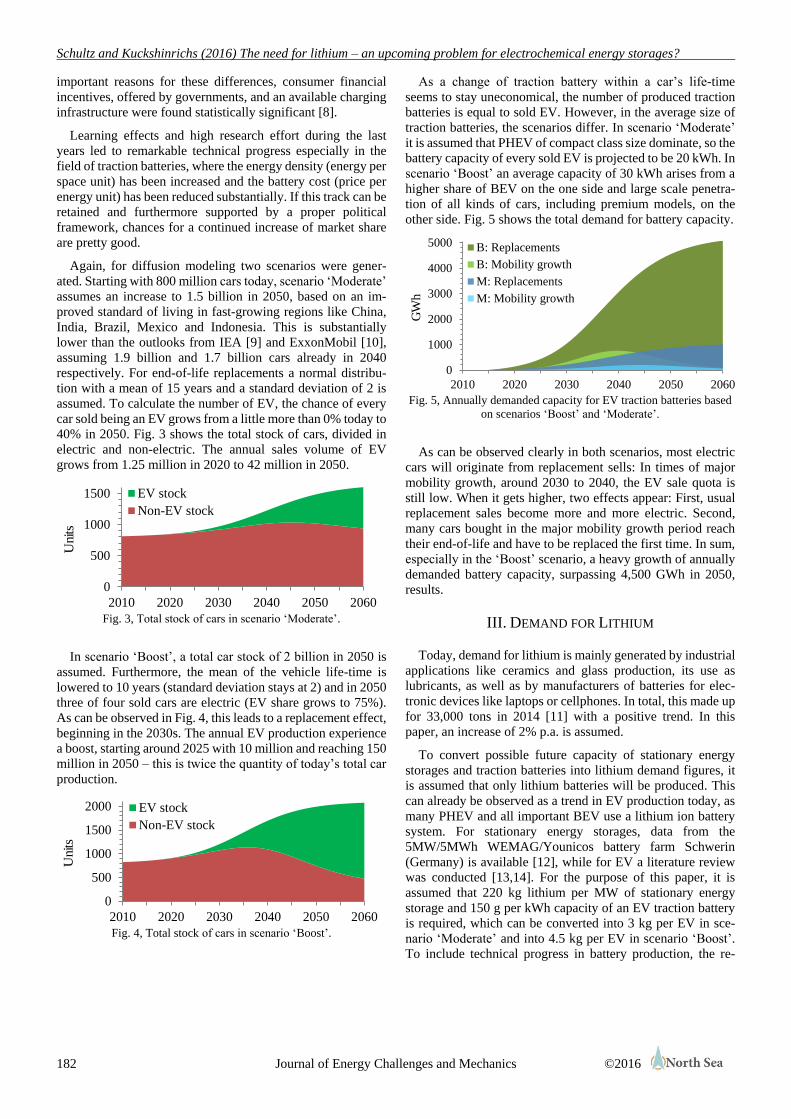
Again, for diffusion modeling two scenarios were gener-
ated. Starting with 800 million cars today, scenario ‘Moderate’
assumes an increase to 1.5 billion in 2050, based on an im-
proved standard of living in fast-growing regions like China,
India, Brazil, Mexico and Indonesia. This is substantially
lower than the outlooks from IEA [9] and ExxonMobil [10],
assuming 1.9 billion and 1.7 billion cars already in 2040
respectively. For end-of-life replacements a normal distribu-
tion with a mean of 15 years and a standard deviation of 2 is
assumed. To calculate the number of EV, the chance of every
car sold being an EV grows from a little more than 0% today to
40% in 2050. Fig. 3 shows the total stock of cars, divided in
electric and non-electric. The annual sales volume of EV
grows from 1.25 million in 2020 to 42 million in 2050.
Fig. 3, Total stock of cars in scenario ‘Moderate’.
In scenario ‘Boost’, a total car stock of 2 billion in 2050 is
assumed. Furthermore, the mean of the vehicle life-time is
lowered to 10 years (standard deviation stays at 2) and in 2050
three of four sold cars are electric (EV share grows to 75%).
As can be observed in Fig. 4, this leads to a replacement effect,
beginning in the 2030s. The annual EV production experience
a boost, starting around 2025 with 10 million and reaching 150
million in 2050 – this is twice the quantity of today’s total car
production.
Fig. 4, Total stock of cars in scenario ‘Boost’.
As a change of traction battery within a car’s life-time
seems to stay uneconomical, the number of produced traction
batteries is equal to sold EV. However, in the average size of
traction batteries, the scenarios differ. In scenario ‘Moderate’
it is assumed that PHEV of compact class size dominate, so the
battery capacity of every sold EV is projected to be 20 kWh. In
scenario ‘Boost’ an average capacity of 30 kWh arises from a
higher share of BEV on the one side and large scale penetra-
tion of all kinds of cars, including premium models, on the
other side. Fig. 5 shows the total demand for battery capacity.
Fig. 5, Annually demanded capacity for EV traction batteries based
on scenarios ‘Boost’ and ‘Moderate’.
As can be observed clearly in both scenarios, most electric
cars will originate from replacement sells: In times of major
mobility growth, around 2030 to 2040, the EV sale quota is
still low. When it gets higher, two effects appear: First, usual
replacement sales become more and more electric. Second,
many cars bought in the major mobility growth period reach
their end-of-life and have to be replaced the first time. In sum,
especially in the ‘Boost’ scenario, a heavy growth of annually
demanded battery capacity, surpassing 4,500 GWh in 2050,
results.
III. DEMAND FOR LITHIUM
Today, demand for lithium is mainly generated by industrial
applications like ceramics and glass production, its use as
lubricants, as well as by manufacturers of batteries for elec-
tronic devices like laptops or cellphones. In total, this made up
for 33,000 tons in 2014 [11] with a positive trend. In this
paper, an increase of 2% p.a. is assumed.
To convert possible future capacity of stationary energy
storages and traction batteries into lithium demand figures, it
is assumed that only lithium batteries will be produced. This
can already be observed as a trend in EV production today, as
many PHEV and all important BEV use a lithium ion battery
system. For stationary energy storages, data from the
5MW/5MWh WEMAG/Younicos battery farm Schwerin
(Germany) is available [12], while for EV a literature review
was conducted [13,14]. For the purpose of this paper, it is
assumed that 220 kg lithium per MW of stationary energy
storage and 150 g per kWh capacity of an EV traction battery
is required, which can be converted into 3 kg per EV in sce-
nario ‘Moderate’ and into 4.5 kg per EV in scenario ‘Boost’.
To include technical progress in battery production, the re-
0
1000
2000
3000
4000
5000
2010 2020 2030 2040 2050 2060
B: Replacements
B: Mobility growth
M: Replacements
M: Mobility growth
GW
h
0
500
1000
1500
2000
2010 2020 2030 2040 2050 2060
EV stock
Non-EV stock
Units
0
500
1000
1500
2010 2020 2030 2040 2050 2060
EV stock
Non-EV stock
Units
Schultz and Kuckshinrichs (2016) The need for lithium – an upcoming problem for electrochemical energy storages?
183 Journal of Energy Challenges and Mechanics ©2016
quired amount of lithium per battery unit of both applications
is lowered by 1% annually.
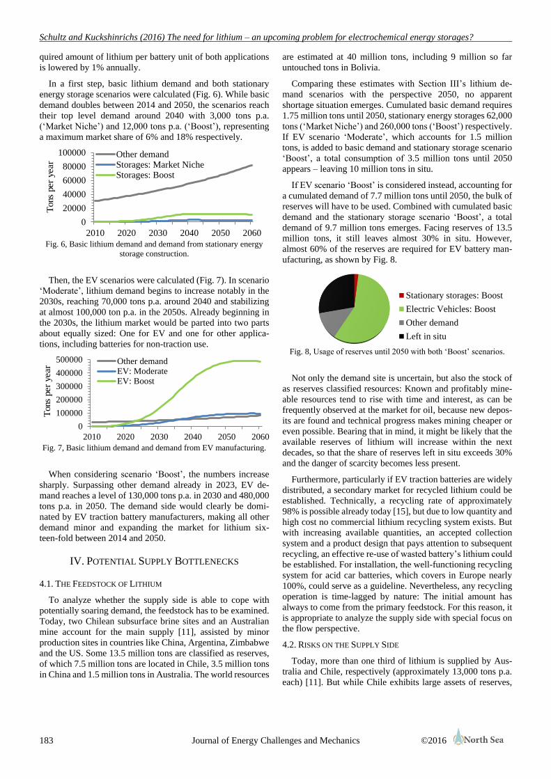
In a first step, basic lithium demand and both stationary
energy storage scenarios were calculated (Fig. 6). While basic
demand doubles between 2014 and 2050, the scenarios reach
their top level demand around 2040 with 3,000 tons p.a.
(‘Market Niche’) and 12,000 tons p.a. (‘Boost’), representing
a maximum market share of 6% and 18% respectively.
Fig. 6, Basic lithium demand and demand from stationary energy
storage construction.
Then, the EV scenarios were calculated (Fig. 7). In scenario
‘Moderate’, lithium demand begins to increase notably in the
2030s, reaching 70,000 tons p.a. around 2040 and stabilizing
at almost 100,000 ton p.a. in the 2050s. Already beginning in
the 2030s, the lithium market would be parted into two parts
about equally sized: One for EV and one for other applica-
tions, including batteries for non-traction use.
Fig. 7, Basic lithium demand and demand from EV manufacturing.
When considering scenario ‘Boost’, the numbers increase
sharply. Surpassing other demand already in 2023, EV de-
mand reaches a level of 130,000 tons p.a. in 2030 and 480,000
tons p.a. in 2050. The demand side would clearly be domi-
nated by EV traction battery manufacturers, making all other
demand minor and expanding the market for lithium six-
teen-fold between 2014 and 2050.
IV. POTENTIAL SUPPLY BOTTLENECKS
4.1. THE FEEDSTOCK OF LITHIUM
To analyze whether the supply side is able to cope with
potentially soaring demand, the feedstock has to be examined.
Today, two Chilean subsurface brine sites and an Australian
mine account for the main supply [11], assisted by minor
production sites in countries like China, Argentina, Zimbabwe
and the US. Some 13.5 million tons are classified as reserves,
of which 7.5 million tons are located in Chile, 3.5 million tons
in China and 1.5 million tons in Australia. The world resources
are estimated at 40 million tons, including 9 million so far
untouched tons in Bolivia.
Comparing these estimates with Section III’s lithium de-
mand scenarios with the perspective 2050, no apparent
shortage situation emerges. Cumulated basic demand requires
1.75 million tons until 2050, stationary energy storages 62,000
tons (‘Market Niche’) and 260,000 tons (‘Boost’) respectively.
If EV scenario ‘Moderate’, which accounts for 1.5 million
tons, is added to basic demand and stationary storage scenario
‘Boost’, a total consumption of 3.5 million tons until 2050
appears – leaving 10 million tons in situ.
If EV scenario ‘Boost’ is considered instead, accounting for
a cumulated demand of 7.7 million tons until 2050, the bulk of
reserves will have to be used. Combined with cumulated basic
demand and the stationary storage scenario ‘Boost’, a total
demand of 9.7 million tons emerges. Facing reserves of 13.5
million tons, it still leaves almost 30% in situ. However,
almost 60% of the reserves are required for EV battery man-
ufacturing, as shown by Fig. 8.
Stationary storages: Boost
Electric Vehicles: Boost
Other demand
Left in situ
Fig. 8, Usage of reserves until 2050 with both ‘Boost’ scenarios.
Not only the demand site is uncertain, but also the stock of
as reserves classified resources: Known and profitably mine-
able resources tend to rise with time and interest, as can be
frequently observed at the market for oil, because new depos-
its are found and technical progress makes mining cheaper or
even possible. Bearing that in mind, it might be likely that the
available reserves of lithium will increase within the next
decades, so that the share of reserves left in situ exceeds 30%
and the danger of scarcity becomes less present.
Furthermore, particularly if EV traction batteries are widely
distributed, a secondary market for recycled lithium could be
established. Technically, a recycling rate of approximately
98% is possible already today [15], but due to low quantity and
high cost no commercial lithium recycling system exists. But
with increasing available quantities, an accepted collection
system and a product design that pays attention to subsequent
recycling, an effective re-use of wasted battery’s lithium could
be established. For installation, the well-functioning recycling
system for acid car batteries, which covers in Europe nearly
100%, could serve as a guideline. Nevertheless, any recycling
operation is time-lagged by nature: The initial amount has
always to come from the primary feedstock. For this reason, it
is appropriate to analyze the supply side with special focus on
the flow perspective.
4.2. RISKS ON THE SUPPLY SIDE
Today, more than one third of lithium is supplied by Aus-
tralia and Chile, respectively (approximately 13,000 tons p.a.
each) [11]. But while Chile exhibits large assets of reserves,
0
100000
200000
300000
400000
500000
2010 2020 2030 2040 2050 2060
Other demandEV: ModerateEV: Boost
Tons
per
year
0
20000
40000
60000
80000
100000
2010 2020 2030 2040 2050 2060
Other demandStorages: Market NicheStorages: Boost
Tons
per
year

Schultz and Kuckshinrichs (2016) The need for lithium – an upcoming problem for electrochemical energy storages?
184 Journal of Energy Challenges and Mechanics ©2016
could be the prospects of expanding Australian supply nar-
rowed. Particularly if EV experiences a boom within a short
time period, raising lithium demand from 33,000 tons today to
180,000 tons in 2030 and further to 560,000 tons in 2050,
other sources will have to be made accessible and developed
quickly and simultaneously. But as can be well observed at the
extraction of unconventional oil, large amounts of capital and
know-how are required for large-scale projects. Adopting this
to the extraction of lithium, several possible risks appear: The
number of professionals could be insufficient, causing a ‘bot-
tleneck of know-how’ and resulting in a slow speed of con-
struction and increased costs for completion.
Moreover, large amounts of capital have to be allocated for
long-term investments. To invest, actors need favorable sur-
rounding conditions at political and economic levels. In the
case of the brine lakes of Bolivia, disposing with approxi-
mated 9 million tons the world’s largest sources, the political
framework could become an issue. Recent acts of nationali-
zation in the telecommunication and even energy sector and
depreciative statements of the Bolivian government directed
against foreign investors are likely to discourage engagement
from outside. A possible result can be observed in allied
Venezuela, where projects for the development of heavy oil
resources achieve only little or no progress at all, because of
missing know-how and capital. If this happens in times with
strongly increasing demand for lithium, the risk for a supply
shortage at the world market will be raised.
Another possible risk on the supply side is based on its
geographic distribution [16]. Today, nearly 60% of the re-
source base is suspected to be located in South American
countries, and due to high Chilean reserves even two-thirds of
the reserves are South American. As most battery and car
manufacturers are located in Europe, Northern America and
Asia, it seems reasonable to expect a high export share for
South American lithium. If one takes the oil market as a
comparison again, one can observe that big net exporters allied
and tried to join forces with the aim of gaining control of the
market; they formed the cartel OPEC, which is responsible for
several world oil crises with periods of lowered supply and
high market prices. If South American net exporting countries
unite with the aim of gaining market control and raising their
profit, and establish a collaboration as well, another risk of
reduced supply on the world market will appear.
In any case, if supply expansion cannot follow an increase
in lithium demand, this can affect applications like stationary
energy storages and electric mobility for two reasons. First,
manufacturers have to cope with a restricted amount of lithium
available, potentially leading to problems within the supply
chain and resulting in production downtimes in the worst case.
Second, the usual market result in situations of supply short-
age is a growing price level. At battery manufacturer’s level,
this is represented by increasing costs for input factors. Espe-
cially for products that are being launched onto the market,
this could become a considerable handicap, with price sensi-
tive customers bailing out as soon as increasing input costs are
forwarded. Today, the price development of lithium is quite
stable [11], but this has not to last forever.
V. CONCLUSION
A simulation model was developed and possible paths of
market penetration for two possibly large-scale applications of
lithium ion batteries were generated. Due to the early market
launch stage of both applications, the scenarios differed to a
large extent. In all scenarios, a major phase of growing pene-
tration was introduced, followed by a phase of leveling. In the
case of stationary energy storages the yearly gross construc-
tion rate rises accordingly, with end-of-life replacements
replacing net constructions. However, in the case of electric
mobility two effects interfere with each other and cause a
strong and massive increase of the production of electric cars.
First, it is expected that the number of cars worldwide will
grow substantially, resulting in EV net constructions. Second,
the share of produced cars being electric increases over time.
This causes the effect of partly replacing the oil fueled car fleet
by electric vehicles, which is due to the high number of cars a
large market as well.
Then, the resulting demand for lithium was calculated and
confronted with today’s lithium demand. It turned out that the
lithium need for stationary energy storages could gain a sound
market share at the world lithium market. Furthermore, and
not surprising, the demand for EV traction batteries has the
potential to revolutionize the lithium market, with being even
the lithium requirements of scenario ‘Moderate’ more than all
other demand summed up. If EV experiences a boom, the
market will change completely and quadruple the first time
until 2030 and another time until 2050.
Analyzing data of known lithium sources, this does not
seem as a major risk in terms of exhausting world reserves,
especially if a market for lithium recycling is introduced. But
with possible strongly rising demand in mind, the authors see
serious potential for risks on the supply side, which may result
in temporary shortage situations and rising price levels at the
lithium world market. First, input factor markets for the con-
struction of depletion facilities could face a shortage, for
example due to a lack of professionals. Second, an unfavorable
investment framework particularly in Bolivia could delay a
sufficient buildup of facilities as well. Third, a collaboration of
net exports located in South America could try to take ad-
vantage of a high market share and ration supply to maximize
profits and/or enforce political objectives.
To counteract those potential future risks, the market for
lithium on the one side and applications for lithium technolo-
gies on the other side should be carefully observed. Further-
more, to keep the recycling option, starting today attention
should be paid to product designs making subsequent disas-
sembling and recycling as easy as feasible. To counter short-
ages in facility construction as well as the time lag between
primary and secondary market, preparatory steps for future
development of today unused deposits could be carried out
already today. In addition, actors could work towards a more
cooperative atmosphere to avoid Bolivian solo attempts in
developing possibly crucial deposits.

Schultz and Kuckshinrichs (2016) The need for lithium – an upcoming problem for electrochemical energy storages?
185 Journal of Energy Challenges and Mechanics ©2016
REFERENCES
[1] H. Weigt. “Germany’s wind energy: The potential for
fossil capacity replacement and cost saving”, Applied
Energy, 86(10), pp. 1857-1863, 2009.
[2] M. Fürsch, S. Hagspiel, C. Jägemann, S. Nagl, D.
Lindenberger, and E. Tröster. “The role of grid exten-
sions in a cost-efficient transformation of the European
electricity system until 2050”, Applied Energy, 104, pp.
642-652, 2013.
[3] O. Egbue; S. Long. “Barriers to widespread adoption of
electric vehicles: An analysis of consumer attitudes and
perceptions”, Energy Policy, 48, pp. 717-729, 2012.
[4] B. Scrosati; J. Garche. “Lithium batteries: Status, pro-
spects and future”, Journal of Power Sources, 195(9), pp.
2419-2430, 2010.
[5] U.S. Department of Energy. “DOE Global Energy
Storage Database”, www.energystorageexchange.org,
2015.
[6] E. Rogers. Diffusion of Innovations. Glencoe, Ill., USA:
Free Press, 1962.
[7] International Energy Agency. Global EV Outlook 2015.
Paris, 2015.
[8] W. Sierzchula, S. Bakker, K. Maat, and B. van Wee.
“The influence of financial incentives and other so-
cio-economic factors on electric vehicle adoption”, En-
ergy Policy, 68, pp. 183-194, 2014.
[9] International Energy Agency. World Energy Outlook
2014. Paris, 2014.
[10] ExxonMobil. The Outlook for Energy: A View to 2040.
Irving, Texas, USA, 2015.
[11] USGS. Mineral commodity summaries 2015. Reston,
Virginia, USA, 2015.
[12] J.C. Koj, A. Schreiber, P. Stenzel, P. Zapp, J. Fleer, I.
Hahndorf. Life Cycle Assessment of a large-scale battery
system for primary control provision. Jülich, Germany,
2014.
[13] S. Konietzko, M. Gernuks. Ressourcenverfügbarkeit von
sekundären Rohstoffen – Potenzialanalyse für Lithium
und Kobalt. LithoRec Final Report, Braunschweig,
Germany, 2011.
[14] H. Vikström, S. Davidsson, M. Höök. “Lithium availa-
bility and future production outlooks”, Applied Energy,
110, pp. 252-266, 2013.
[15] J.H. Miedema, H.C. Moll. “Lithium availability in the
EU27 for battery-driven vehicles: The impact of recy-
cling and substitution on the confrontation between
supply and demand until 2050”, Resources Policy, 38, pp.
204-211, 2013.
[16] C. Grosjean, P.H. Miranda, M. Perrin, P. Poggi. “As-
sessment of world lithium resources and consequences of
their geographic distribution on the expected develop-
ment of the electric vehicle industry”, Renewable and
Sustainable Energy Reviews, 16, pp. 1735-1744, 2012.

ISSN 2056-9386
Volume 3 (2016) issue 4, article 3
186 ©2016
A GIS-based statistical approach to prioritize the
retrofit of housing stocks at the urban scale
基于地理信息系统的统计方法用于城市规模住房存量
改造的优先等级处理
Alessio Mastrucci1*, Olivier Baume2, Francesca Stazi3, Ulrich Leopold4
1International Institute for Applied Systems Analysis, Schlossplatz 1, A-2361 Laxenburg, Austria 2Resource Centre for Environmental Technologies - Public Research Centre Henri Tudor, 6A, avenue des Hauts-Fourneaux,
L-4362 Esch-sur-Alzette, Luxembourg 3Dipartimento di Ingegneria Civile, Edile e Architettura - Universita Politecnica delle Marche, Via Brecce Bianche 12, 60131
Ancona, Italy 4Luxembourg Institute of Science and Technology, 5 avenue des Hauts-Fourneaux, L-4362 Esch-sur-Alzette
[email protected] (Alessio Mastrucci); [email protected] (Ulrich Leopold)
Abstract - Cities are responsible for about 70% of the overall
primary energy consumption in Europe and play a major role in
addressing carbon mitigation. In this respect, the housing sector
has been identified as a key sector for its high energy savings
potential achievable by implementing retrofit measures. However,
a detailed characterization of the housing energy consumption
profile and spatial distribution is needed to properly assess the
energy saving potential at the urban scale and further support
sustainable urban planning and energy policies.
This study focused on a statistical approach based on
Geographical Information Systems (GIS) developed to identify
the energy consumption profile of urban housing stocks, the
energy savings potential achievable by implementing retrofit
measures and their respective spatial distribution across one
entire city. The final energy consumption of individual dwellings
is predicted by running a multiple linear regression model based
on measured energy consumption available at aggregated level
(post-code area level) and GIS data about characteristics of
buildings and household. Energy savings potential and cost-
effectiveness of standard retrofit measures are subsequently
calculated and results are finally displayed as maps for decision
support in sustainable urban planning. The methodology was
applied to the exemplary housing stock of Rotterdam city,
consisting of almost 300,000 units.
Relevant results are provided to prioritize retrofit measures
implementation according to energy savings potential and cost-
effectiveness. Different types of maps can be produced to show
energy consumption and energy saving potential patterns across
the city. The methodology is generically applicable to other
contexts and provides an effective tool for decision support in
carbon mitigation policies of housing stocks at the urban scale.
Keywords – Building stock; Energy savings; Costs; Sustainable
urban planning.
I. INTRODUCTION
Cities play a major role in addressing carbon mitigation as
they are responsible for about 70% of the overall primary
energy consumption in Europe [1]. A significant part of the
energy consumption and greenhouse gases emission of cities
is attributable to the building sector. As a consequence, the
European Directive 2012/27/EU[2] required the Member
States a long term strategy for mobilizing investment in this
sector. In particular, the housing sector has been identified as
one of those with the highest energy savings potential
achievable through the implementation of retrofit measure.
However, a detailed characterization of the housing energy
consumption profile and spatial distribution is needed to
properly assess the energy savings potential at the urban scale
and further support sustainable urban planning and energy
policies. Several types of bottom-up housing stock models
have been developed to this end [3]. Statistical models use
historical data to attribute final energy consumption to single
or groups of buildings using a range of statistical techniques.
Even though statistical models are limited in predicting the
impact of new technologies, they can efficiently be used to
estimate the actual energy consumption profile of the building
stock including the effect of the real state of renovation and
behavior of occupants. A few statistical models have been
already developed for the housing sector, however there is a

Mastrucci et al. (2016) A GIS-based statistical approach to prioritize the retrofit of housing stocks at the urban scale
187 Journal of Energy Challenges and Mechanics ©2016
lack of studies at the urban scale and taking into account the
spatial distribution of energy consumption [4].
The objective of this study was to identify the energy
savings and CO2 reduction potential of retrofit measures for
urban housing stocks in order to prioritize their
implementation across one entire city also using cost-
effectiveness criteria. A statistical approach based on
Geographical Information Systems (GIS) was developed for
this scope. The final energy consumption of individual
dwellings was predicted by running a multiple linear
regression model based on measured energy consumption
available at aggregated level (post-code area level) and GIS
data about characteristics of buildings and households. Energy
savings potential and cost-effectiveness of standard retrofit
measures were subsequently computed using benchmark
values and results were finally displayed as maps for decision
support in sustainable urban planning.
The methodology was developed as part of the European
INTERREG IVB NEW project MUSIC [5] to be implemented
into the web-based integrated decision support platform
iGUESS [6].
II. CASE STUDY
The housing stock of Rotterdam city, counting 297,312
dwellings in 2012, was taken as a case study. Six typologies of
dwellings can be identified, distributed into houses (detached,
semi-detached, row-houses) and apartments (maisonette,
“galerij” flats, “portiek” flats). Houses account for 24% of the
total number of dwellings in Rotterdam with a predominance
of row-houses (16%) and a minor share of semi-detached (7%)
and detached houses (1%). Apartments represent about 76% of
the stock divided into maisonettes (22%), galerij flats (19%)
and portiek flats (35%). About 51% of the dwellings were
built before 1965, 10% in the period 1965-74, 23% in 1975-
1991 and 13% in 1991-2005.
The main energy carrier for space heating, domestic hot
water and hob cooking is natural gas, while about 17% of
dwellings are connected to the urban heating network.
Electricity is mainly used for lighting and appliances and
partly for domestic hot water.
Data about dwellings and households were extracted from
the GIS address database of the Municipality, including
information about floor surface, type of dwelling and period of
construction, number of occupants. Measured natural gas
consumption are available on a yearly basis at the post-code
area level. National building libraries and standards [7,8] were
used to apportion the total energy consumption into different
end-uses and to estimate the energy saving potential and
investment costs for standard retrofit packages.
III. METHODOLOGY
A bottom-up statistical approach based on GIS was
developed at the city scale to predict the final energy
consumption of the housing stock [4]. Multiple linear
regression is used to disaggregate measured natural gas
consumption values available at post-code area level to single
dwellings depending on building and household features. The
equation at the basis of the model for gas is Eq (1):
y = β0 + xfloor βfloor +Σi xtype,i βtype,i + ε (1)
where the dependent variable y represents measured yearly
average gas consumption per dwelling at post-code level, the
independent variable xfloor the average floor surface of
dwellings, xtype,i the percentage of dwellings per type and
period of construction (26 combinations) in the post-code, β0,
βfloor, βtype,i the regression coefficients to be estimated
commonly by ordinary least squares technique and ε a random
error term. The residuals were carefully analyzed and their
spatial distribution displayed at post-code level so to identify
areas with higher consumption deviation and detect possible
spatial patterns. The software QGIS [9] was used for this scope.
The total natural gas consumption was apportioned into
different end uses and the energy savings potential and costs
of standard retrofit measures were calculated based on national
benchmark values and standards [7,8]. Standard retrofit
packages include isolation of external walls, roof and ground
floor, windows replacement and boiler replacement according
to Dutch regulations (Table 1).
An index to evaluate the cost-effectiveness of retrofit
measures Cen.sav (€ / kWh a) was defined according to Eq (2):
Cen.sav= Iretr / Esav (2)
where Iretr (€) is the investment cost of the standard retrofit
measure package and Esav (kWh) is the yearly energy savings
potential. Such index is suitable to prioritize the
implementation of retrofit measures for residential buildings
across the city.
TABLE 1, STANDARD RETROFIT PACKAGES FOR THE BUILDING
ENVELOPE IN THE NETHERLANDS (ADAPTED FROM [7]).
Retrofit package U-value
(kWh/m2K)
Rc-value
(m2K/kWh)
External wall insulation 0.36 2.53
Roof insulation 0.36 2.53
Ground floor insulation 0.36 2.53
Double Glazing LowE - HR++ 1.80 -
Energy consumption and energy savings predicted for single
dwellings were aggregated across the city at the block level
and their distribution was spatially analyzed using GIS. The
block level was selected as the target level where to show
information useful for decision support in urban planning as
this level gives sufficient detail in results and at the same time
keeps sensitive data protected (e.g. information for single
buildings). Maps were generated at the block level for the total
primary energy consumption for space heating and domestic
hot water in the current state, the total energy savings potential
achievable through standard retrofit measures and the average
cost of energy savings.
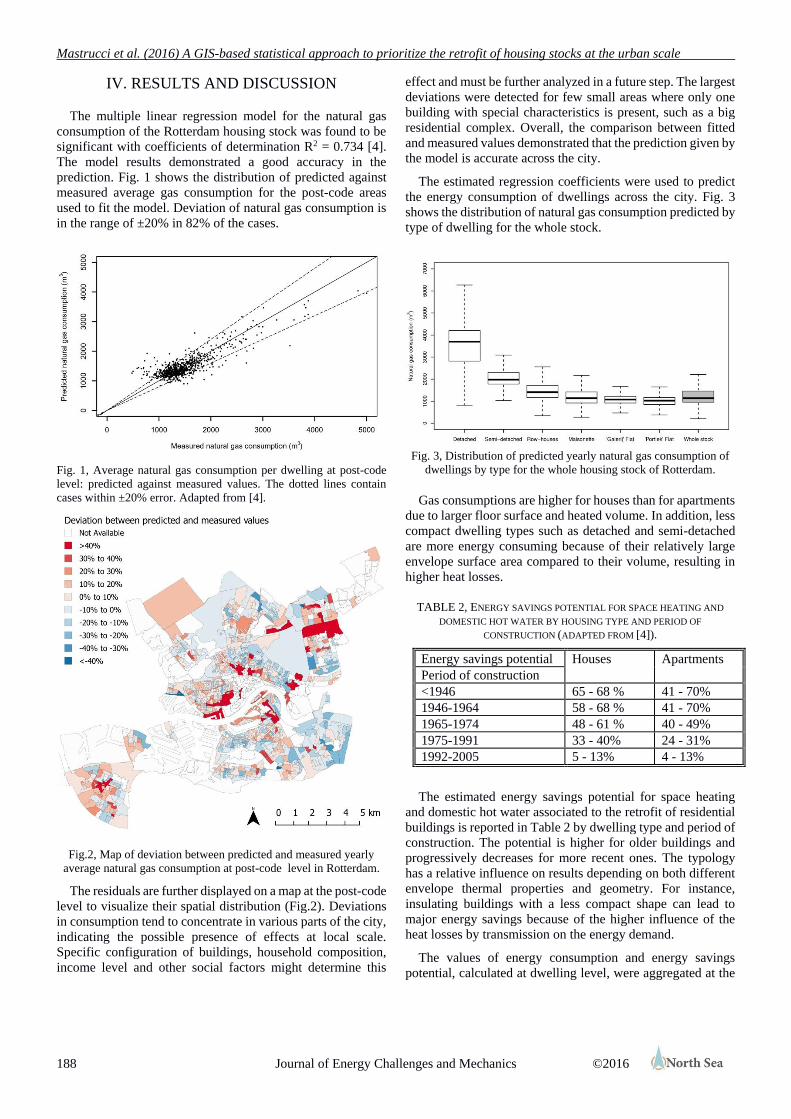
Mastrucci et al. (2016) A GIS-based statistical approach to prioritize the retrofit of housing stocks at the urban scale
188 Journal of Energy Challenges and Mechanics ©2016
IV. RESULTS AND DISCUSSION
The multiple linear regression model for the natural gas
consumption of the Rotterdam housing stock was found to be
significant with coefficients of determination R2 = 0.734 [4].
The model results demonstrated a good accuracy in the
prediction. Fig. 1 shows the distribution of predicted against
measured average gas consumption for the post-code areas
used to fit the model. Deviation of natural gas consumption is
in the range of ±20% in 82% of the cases.
Fig. 1, Average natural gas consumption per dwelling at post-code
level: predicted against measured values. The dotted lines contain
cases within ±20% error. Adapted from [4].
Fig.2, Map of deviation between predicted and measured yearly
average natural gas consumption at post-code level in Rotterdam.
The residuals are further displayed on a map at the post-code
level to visualize their spatial distribution (Fig.2). Deviations
in consumption tend to concentrate in various parts of the city,
indicating the possible presence of effects at local scale.
Specific configuration of buildings, household composition,
income level and other social factors might determine this
effect and must be further analyzed in a future step. The largest
deviations were detected for few small areas where only one
building with special characteristics is present, such as a big
residential complex. Overall, the comparison between fitted
and measured values demonstrated that the prediction given by
the model is accurate across the city.
The estimated regression coefficients were used to predict
the energy consumption of dwellings across the city. Fig. 3
shows the distribution of natural gas consumption predicted by
type of dwelling for the whole stock.
Fig. 3, Distribution of predicted yearly natural gas consumption of
dwellings by type for the whole housing stock of Rotterdam.
Gas consumptions are higher for houses than for apartments
due to larger floor surface and heated volume. In addition, less
compact dwelling types such as detached and semi-detached
are more energy consuming because of their relatively large
envelope surface area compared to their volume, resulting in
higher heat losses.
TABLE 2, ENERGY SAVINGS POTENTIAL FOR SPACE HEATING AND
DOMESTIC HOT WATER BY HOUSING TYPE AND PERIOD OF
CONSTRUCTION (ADAPTED FROM [4]).
Energy savings potential Houses Apartments
Period of construction
<1946 65 - 68 % 41 - 70%
1946-1964 58 - 68 % 41 - 70%
1965-1974 48 - 61 % 40 - 49%
1975-1991 33 - 40% 24 - 31%
1992-2005 5 - 13% 4 - 13%
The estimated energy savings potential for space heating
and domestic hot water associated to the retrofit of residential
buildings is reported in Table 2 by dwelling type and period of
construction. The potential is higher for older buildings and
progressively decreases for more recent ones. The typology
has a relative influence on results depending on both different
envelope thermal properties and geometry. For instance,
insulating buildings with a less compact shape can lead to
major energy savings because of the higher influence of the
heat losses by transmission on the energy demand.
The values of energy consumption and energy savings
potential, calculated at dwelling level, were aggregated at the

Mastrucci et al. (2016) A GIS-based statistical approach to prioritize the retrofit of housing stocks at the urban scale
189 Journal of Energy Challenges and Mechanics ©2016
block level and displayed as spatial maps for the entire city of
Rotterdam (Figs. 4-5).
Fig.4, Map of primary energy consumption at block level for space
heating and domestic hot water of dwellings across Rotterdam.
Fig. 4 displays maps of primary energy consumption for
space heating and domestic hot water of dwellings across the
whole city. Higher energy consumption is registered for the
city center and adjacent areas characterized by high density
and the presence of older flats and row-houses. In contrast, the
city suburbs have total lower energy consumption due to a
lower density, despite the presence of detached and semi-
detached houses more energy consuming.
Fig.5, Map of energy savings potential at the block level for space
heating and domestic hot water of dwellings across Rotterdam.
Fig. 6, Map of cost of yearly energy savings at the block level for
space heating and domestic hot water of dwellings across
Rotterdam.
The map in Fig. 5 shows the energy savings potential for
combined space heating and domestic hot water achievable
through the implementation of typical retrofit measures for
buildings. The map is suitable to identify across the city areas
where the retrofit of residential buildings is more promising in
terms of energy savings. These areas are characterized by a
dense urban tissue and the predominance of old buildings.
A map was drawn at the block level to show the cost-
effectiveness of retrofit measures across the city (Fig. 6). The
cost of energy savings depends on the type and period of
construction of dwellings present in a specific area. Lower cost
values indicate higher cost-effectiveness of retrofitting. The
cost of energy savings decreases for older buildings, indicating
an higher cost-effectiveness of retrofit measures (Table 3).
The areas of Rotterdam where the distributed retrofit is
expected to be more cost-effective are mainly located in the
belt around the city center and in some of the suburbs where
the presence of older buildings is larger. However, by
comparison of this map (Fig. 6) with the energy savings
potential map (Fig. 5) it emerges that not every area where the
retrofit is more cost-effective has a large energy savings
potential. This depends mainly on the urban density, for
instance areas in the outskirts with old detached houses and
low density tissue, have high cost-effectiveness values for
retrofit but low energy savings potential. The two maps can be
used in combination to support decision and prioritization of
retrofit measures across the city.
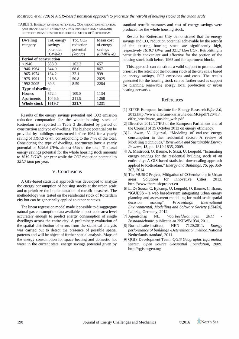
Mastrucci et al. (2016) A GIS-based statistical approach to prioritize the retrofit of housing stocks at the urban scale
190 Journal of Energy Challenges and Mechanics ©2016
TABLE 3, ENERGY SAVINGS POTENTIAL, CO2 REDUCTION POTENTIAL
AND MEAN COST OF ENERGY SAVINGS IMPLEMENTING STANDARD
RETROFIT MEASURES FOR THE HOUSING STOCK OF ROTTERDAM.
Dwelling
category
Tot. energy
savings
potential
(GWh/a)
Tot. CO2
reduction
potential
(kton/a)
Mean cost
of energy
savings
(€/MWh /a)
Period of construction
<1946 853.0 162.2 657
1946-1964 344.9 68.0 867
1965-1974 164.2 32.1 939
1975-1991 218.3 50.8 2025
1992-2005 39.3 8.59 2284
Type of dwelling
Houses 572.4 109.8 1134
Apartments 1046.6 211.9 1268
Whole stock 1619.7 321.7 1231
Results of the energy savings potential and CO2 emission
reduction computation for the whole housing stock of
Rotterdam are reported in Table 3 distributed by period of
construction and type of dwelling. The highest potential can be
provided by buildings constructed before 1964 for a yearly
saving of 1197,9 GWh, corresponding to the 74% of the total.
Considering the type of dwelling, apartments have a yearly
potential of 1046.6 GWh, almost 65% of the total. The total
energy savings potential for the whole housing stock amounts
to 1619.7 GWh per year while the CO2 reduction potential to
321.7 kton per year.
V. Conclusions
A GIS-based statistical approach was developed to analyze
the energy consumption of housing stocks at the urban scale
and to prioritize the implementation of retrofit measures. The
methodology was tested on the residential stock of Rotterdam
city but can be generically applied to other contexts.
The linear regression model made it possible to disaggregate
natural gas consumption data available at post-code area level
accurately enough to predict energy consumption of single
dwellings across the entire city. A preliminary evaluation of
the spatial distribution of errors from the statistical analysis
was carried out to detect the presence of possible spatial
patterns and will be object of further spatial analysis. Maps of
the energy consumption for space heating and domestic hot
water in the current state, energy savings potential given by
standard retrofit measures and cost of energy savings were
produced for the whole housing stock.
Results for Rotterdam City demonstrated that the energy
savings and CO2 reduction potential achievable by the retrofit
of the existing housing stock are significantly high,
respectively 1619.7 GWh and 321.7 kton CO2 . Retrofitting is
particularly convenient and effective for the portion of the
housing stock built before 1965 and for apartment blocks.
This approach can constitute a valid support to promote and
prioritize the retrofit of the housing stock at the city scale based
on energy savings, CO2 emissions and costs. The results
generated for the housing stock can be further used as support
for planning renewable energy local production or urban
heating networks.
References
[1] EIFER European Institute for Energy Research.Eifer 2.0,
2012.http://www.eifer.uni-karlsruhe.de/IMG/pdf/120417_
eifer_broschuere_ansicht_web.pdf
[2] Directive 2012/27/EU of the European Parliament and of
the Council of 25 October 2012 on energy efficiency.
[3] L. Swan, V. Ugursal, “Modeling of end-use energy
consumption in ther residential sector: A review of
Modeling techniques,” Renewable and Sustainable Energy
Reviews, 13, pp. 1819-1835, 2009.
[4] A. Mastrucci, O. Baume, F. Stazi, U. Leopold. “Estimating
energy savings for the residential building stock of an
entire city: A GIS-based statistical downscaling approach
applied to Rotterdam,” Energy and Buildings, 75, pp. 358-
367, 2014.
[5] The MUSIC Project, Mitigation of CO2emissions in Urban
areas: Solutions for Innovative Cities, 2013.
http://www.themusicproject.eu
[6] L. De Sousa, C. Eykamp, U. Leopold, O. Baume, C. Braun.
“iGUESS – a web basedsystem integrating urban energy
planning and assessment modelling for multi-scale spatial
decision making”, Proceedings International
Environmental, Modelling and Software Society (iEMSs),
Leipzig, Germany, 2012.
[7] Agentschap NL, Voorbeeldwoningen 2011 -
Bestaandebouw, publicatie-nr.2KPWB1034, 2011.
[8] Normalisatie-instituut, NEN 7120:2011. Energy
performance of buildings -Determination method.National
Netherlands standard, 2011.
[9] QGIS Development Team. QGIS Geographic Information
System, Open Source Geospatial Foundation, 2009.
http://qgis.osgeo.org

ISSN 2056-9386
Volume 3 (2016) issue 4, article 4
191 ©2016
Parametric modeling of producer gas-combustor and
heat exchanger integration for micro-gas turbine
application
发生气参数化建模 – 用于微型燃气轮机之燃烧器与热
交换器集成
Mackay A.E. Okure1, Wilson B. Musinguzi2*, Terese Løvås3
1School of Engineering, Makerere University, P.O. Box 7062, Kampala, Uganda 2Faculty of Engineering, Busitema University, P.O. Box 236, Tororo, Uganda
3Department of Energy and Process Engineering, NTNU, Trondheim, Norway
*Corresponding Author: [email protected]
Accepted for publication on 14th September 2016
Abstract - An alternative way of improving the use of biomass
resources in rural areas of developing countries is to design
suitable combined heat, and power (CHP) small-scale plants for
distributed generation. A gasification-based CHP system can
potentially have higher electricity efficiency than a direct
combustion-based CHP system. The combustible gas from wood
gasification is fired in a combustor that is integrated with a heat
exchanger to facilitate effective heat transfer from the hot flue
gases to the 100kWe micro gas turbine working fluid. Burning a
gas in the combustor has an edge over the solid biomass because
the gaseous fuel offers high heat exchanger temperature as well
as stable combustion/continuous operation. Two parameters that
have potential for efficiency advancement are investigated in this
work: increased turbine inlet temperature and heat exchanger
effectiveness. This paper presents a parametric model analysis of
the combustion process in the combustor and heat transfer to the
turbine working medium across the heat exchanger. Aspen Plus
Process Modeling software (aspenONE® Engineering for
Universities V7.3) was used for implementation and performing
sensitivity analysis of the system. The heat exchanger and
combustor integration process analysis has also shown good
performance with the flue gases from combustion of producer
gas providing sufficient thermal energy needed to raise the
turbine working fluid to the required turbine inlet temperature.
The analysis of the heat exchanger has provided parameters
essential for decision making on the sizing of the heat exchanger.
The practical value added was revealing the parameters needed
in the design specification of the heat exchanger suitable for the
heat duty of a typical 100kWe externally fired micro gas turbine
based on gasification of biomass and subsequent producer gas
combustion. The heat exchanger effectiveness of 0.635 was
achieved in this parametric study. Furthermore, the results
revealed that the heat exchanger effectiveness increased with
decrease in adiabatic flame temperature. The heat duty of the hot
combustion gases plays a role in the value of the adiabatic flame
temperature that can give a desired effectiveness and at the same
time satisfy the heat balance between the two streams.
Keywords - Parametric modeling, Producergas-Combustor, Heat
Exchanger, Indirectly Fired Micro-gas Turbine.
I. INTRODUCTION
An alternative way of improving the use of biomass
resources in rural areas of developing countries is to design
suitable combined heat and power (CHP) small-scale plants
for distributed generation. Among solid biomass
thermochemical conversion processes, combustion is the most
advanced and market-proven one, while pyrolysis and
gasification can still be considered to be at a pre-commercial
stage of development according to Maraver et al. [1]. A
gasification-based CHP system can potentially have higher
electricity efficiency than a direct combustion-based CHP
system as demonstrated in [2]-[4]. Another of its advantages is
that gas firing produces less CO2 per unit power than does a
liquid or solid fuel as shown by Pilavachi [5]. According to
Leilei et al. [2], small-scale biomass-fuelled CHP systems
have a particularly strong relevance in improving the quality
of life, especially in rural communities in developing
countries. The first step in designing a CHP plant is to
determine the best configuration in terms of the
thermodynamic integration of all the subsystems and the

Musinguzi et al. (2016) Parametric Modeling of Producergas-Combustor and Heat Exchanger Integration for …
192 Journal of Energy Challenges and Mechanics ©2016
optimization of the overall energy efficiency. Bassily [6]
reports the main methods for improving the efficiency or
power of the combined cycle as: increasing the turbine inlet
temperature (TIT), inlet air-cooling, applying gas reheat,
steam or water injection into the gas turbine (GT), and
reducing the irreversibility of the heat recovery steam
generator (HRSG).
By replacing the combustion chamber of a gas turbine with
a high temperature heat exchanger, the electrical efficiency of
a solid biomass fuelled power plant can be increased from
15-20% to 25-30% [7] for typical plant sizes of 100 kWel. The
main reasons why hot air gas turbines (HGT) have not
succeeded until now are the high operating air temperature of
over 850oC, ash sintering, slagging and fouling, material
problems on the heat exchanger due to the low heat transfer of
flue gas to air and large heat exchanger areas required as
reported by Gaderer et al. [8]. In most applications, heat
exchangers are very important to the overall efficiency, cost,
and size of the system. Current heat exchanger designs rely
heavily on fin-and-tube or plate heat exchanger designs, often
constructed using copper and aluminum. Recent developments
in material science, including advances in ceramics and
ceramic matrix composites, open opportunities for new heat
exchanger designs; Sommers et al. [9]. The major factors
affecting heat exchanger performance are effectiveness,
pressure drop and leakage of the heat transfer medium.
For process intensification, steam injection into the turbine
working medium has shown greater increase in efficiency of
externally fired microturbines due to increased specific heat of
the turbine working medium. Delattin et al. [10] reports that
steam addition of up to the surge limit of 3.3% of the mass of
air flowing into the microturbine can increase the electric
efficiency by 5%.
This paper reports on the parametric modeling of the high
temperature heat exchanger and combustor integration
utilizing a combustible gas from a wood gasifier for improved
heat transfer to the turbine working medium. Thus the heat
exchanger effectiveness is a key parameter to analyze.
II. MATERIALS AND METHODS
The researchers modeled the heat exchanger and combustor
integration and analyzed its performance theoretically. The
authors have carried out parametric modeling of the system to
reveal the relationship of different parameters in the system in
order to achieve the desired output of heat transferred to the
turbine working fluid. The turbine inlet parameters are
specified by the design model chosen and thus the turbine inlet
temperature is set at 950oC. Attempt to have the highest
possible practical value of the key parameter of heat exchanger
effectiveness and thus high heat transfer to the turbine medium
was made in the analysis.
Fig. 1 illustrates the system modeled in this paper. The hot
wood gas from the gasifier and preheated combustion air enter
the combustor integrated with the heat exchanger. The high
temperature combustion gases flow through the shell-side of
the chamber packed with heat exchanger tubes carrying the
turbine working medium (air plus a small amount of steam).
The heated tube-side stream is led to the gas turbine for power
generation. The exhaust from the turbine is led to the heat
recovery steam generator (HRSG) which delivers the steam
needed for injection into compressed air at the right
compressor outlet pressure. The mixing takes place at
common pressure. The exhaust from combustion is used for
combustion air preheating.
Thermodynamic chemical equilibrium analysis of the
combustor was carried out using the RGibbs reactor. This type
of reactor uses the method of direct minimization of Gibbs free
energy. It is useful when the reaction stoichiometry is not
known or is high in number due to many components
participating in the reaction. This is the only Aspen Plus block
that deals with solid, liquid and gas phase equilibrium. For the
heat exchanger, the HEATX block was used for shell-and tube
analysis of the flow. Both the equation of state and ideal
property methods were used in the simulation to compute the
thermodynamic and flow properties of the streams. The
producer fuel properties in Table I published by the authors in
earlier work, were used for the modeling [11], [12].
Process optimization, under atmospheric combustion and
heat exchange, used thermodynamic equilibrium and exergy
analysis. Aspen Plus Process Modeling software (aspenONE®
Engineering for Universities V7.3) was used for
implementation and performing sensitivity analysis of the
system. The thermodynamic analysis of this system considers
continuous deterministic steady-state conditions. Stepwise
procedure with simulation using
ASPEN PLUS process modeling is used in the
thermodynamic analysis of the cycle. The ASPEN PLUS
Gibbs reactor was used for combustion with the assumption
that the reaction follows the Gibbs equilibrium. The process
parameters in the analysis were correlated with those available
in the literature by Schuster et al. [13], Kentaro et al. [14],
Chiaramonti et al. [15], Kautz et al. [7], Daniele et al. [16],
Lieuwen et al. [17]. These parameters represent commercially
available technologies or processes in advanced development
stage.

Musinguzi et al. (2016) Parametric Modeling of Producergas-Combustor and Heat Exchanger Integration for …
193 Journal of Energy Challenges and Mechanics ©2016
Fig. 1, Schematic of the system under study.
III. DERIVATION OF THE PARAMETRIC
MODEL OF THE COMBUSTOR AND
HEAT EXCHANGER
A number of important practical issues must be addressed in
designing a wood gas combustion system in order to achieve
sufficient stability in the operation of the combustor/heat
exchanger combination. Indeed complex interactions between
combustion phenomena and fluid mechanics have been
sighted as not well understood [17]. In particular, burners
involve complex, less understood interactions between
swirling flow dynamics, flow field alterations induced by
volumetric expansion across the flame, and flame propagation.
Unlike in natural gas combustion where premixed burners
are used, combustion of wood gas from the gasifier favorably
utilizes non-premixed burners as portrayed by the majority of
the fundamental investigations on wood gas (syngas)
combustion characteristics [17]. The non-premixed burners
preferred in wood gas combustion are believed to significantly
lower the operability issues that are detrimental to safe
combustion. This study therefore exams two important
parameters namely adiabatic flame temperature and heat
exchanger effectiveness as theoretical basis for the interaction
between the combustor and heat exchanger system.
3.1 Adiabatic Flame Temperature
For purposes of analysis, it is assumed that the combustor
operates at steady-state, steady flow conditions and that in this
case, no work or power transfer occurs in addition to
negligible changes in kinetic and potential energy fluxes.
Energy transfer from the generated gases as heat to the
surroundings (heat exchanger surfaces) due to combustion can
be partly influenced by the properties of fuel burned,
equivalent ratio, state of reactants (fuel and oxidant
phase/temperature) and product state (completeness of
combustion and product temperature) [18]. The adiabatic
flame temperature gives insights on the maximum possible
temperature in the combustor zone so that proper materials for
combustor surfaces can be chosen for a given combustion
Table I, Characteristic properties of the Producer gas generated in a downdraft fixed bed gasifier [11], [12].
Property Value
Wood feed rate 0.02 (kg/s)
Steam (gasifying medium) flow rate at 500oC, 1 bar 0.012 (kg/s)
Reactor temperature in the gasification zone 820 (oC)
Net producer gas flow from the gasifier 0.028 (Nm3/s)
Component distribution in the wood gas 43.27% H2, 14.42% CO, 7.84% CH4,17.31% CO2,
17.16% H2O (mol(%)/mol of wood gas)
HHV of gaseous fuel 13.9 (MJ/kg)
LHV of gaseous fuel 13.4 (MJ/kG)
pgm 0.02 (kg/s)
Sintering temperature of the carry-over ash in wood gas 1334 (oC)
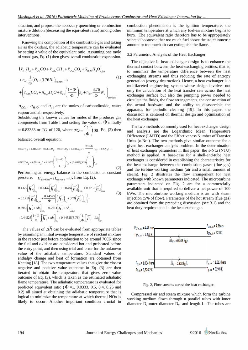
Musinguzi et al. (2016) Parametric Modeling of Producergas-Combustor and Heat Exchanger Integration for …
194 Journal of Energy Challenges and Mechanics ©2016
situation, and propose the necessary quenching or combustion
mixture dilution (decreasing the equivalent ratio) among other
interventions.
Knowing the composition of the combustible gas and taking
air as the oxidant, the adiabatic temperature can be evaluated
by setting a value of the equivalent ratio. Assuming one mole
of wood gas, Eq. (1) then gives overall combustion expression.
product
airairOHCO
oxidantair
fuelOHCOCHCOH
NnOnOHnCOn
NOn
OHxCOxCHxCOxHx
2222
22
2242
76.31
76.31
22
2242
(1)
2COn , OHn2
and airn are the moles of carbondioxide, water
vapour and air respectively.
Substituting the known values for moles of the producer gas
components from Table I and setting the value of initially
at 0.83333 or TO of 120, where 1001
TO , Eq. (2) then
balanced overall equation:
2
1
)76.3)(44525.0(2
)1(
44525.02
7611.02
3957.0
)2
76.32
(
44525.0
21716.0
21731.0
40784.01442.0
24327.0
NOOHCO
NOOHCOCHCOH
(2)
Performing an energy balance in the combustor at constant
pressure; 0tan tsreacproducts HH , from Eq. (2),
2
0
2
0
2
0
2
0
2
0
2
0
2
0
2
0
4
00
2
0
1)76.3(44525.0
144525.0
7611.03957.0
76.344525.0
1716.0
1731.00784.01442.04327.0
Nf
Of
OHf
COf
Nf
Of
OHf
COf
CHf
COf
Hf
hh
hh
hh
hh
hhh
hhhh
(3)
The values of h can be evaluated from appropriate tables
by assuming an initial average temperature of reactant mixture
in the reactor just before combustion to be around 700K since
the fuel and oxidant are considered hot and preheated before
the entry point, and then using trial-and-error for the unknown
value of the adiabatic temperature. Standard values of
enthalpy change and heat of formation are obtained from
Keating [18]. The two temperature values that give the closest
negative and positive value outcome in Eq. (3) are then
iterated to obtain the temperature that gives zero value
outcome of Eq. (3), which is taken as the estimated adiabatic
flame temperature. The adiabatic temperature is evaluated for
predicted equivalent ratio ( =1, 0.8333, 0.5, 0.4, 0.25 and
0.2) all aimed at obtaining the adiabatic temperature that is
logical to minimize the temperature at which thermal NOx is
likely to occur. Another important condition crucial in
combustion phenomenon is the ignition temperature; the
minimum temperature at which any fuel-air mixture begins to
burn. The equivalent ratio therefore has to be appropriately
selected because either too much fuel above the stoichiometric
amount or too much air can extinguish the flame.
3.2 Parametric Analysis of the Heat Exchanger
The objective in heat exchanger design is to enhance the
thermal contact between the heat-exchanging entities, that is,
to minimize the temperature difference between the heat
exchanging streams and thus reducing the rate of entropy
generation (exergy destruction). Hence, a heat exchanger is a
multifaceted engineering system whose design involves not
only the calculation of the heat transfer rate across the heat
exchanger surface but also the pumping power needed to
circulate the fluids, the flow arrangements, the construction of
the actual hardware and the ability to disassemble the
apparatus for periodic cleaning [19]. In this paper, the
discussion is centered on thermal design and optimization of
the heat exchanger.
The two methods commonly used for heat exchanger design
and analysis are the Logarithmic Mean Temperature
Difference (LMTD) and the Effectiveness Number of Transfer
Units (ε-Ntu). The two methods give similar outcome for a
given heat exchanger analysis problem. In the determination
of heat exchanger parameters in this paper, the ε-Ntu (NTU)
method is applied. A base-case for a shell-and-tube heat
exchanger is considered in establishing the characteristics for
the heat exchange between the combustion gases (flue gas)
and the turbine working medium (air and a small amount of
steam). Fig. 2 illustrates the flow arrangement for heat
exchange with known parameters indicated. The microturbine
parameters indicated on Fig. 2 are for a commercially
available unit that is required to deliver a net power of 100
kWe. The microturbine working medium is air with steam
injection (5% of flow). Parameters of the hot stream (flue gas)
are obtained from the preceding discussion (sec 3.1) and the
heat duty requirements in the heat exchanger.
Fig. 2, Flow streams across the heat exchanger.
Compressed air and steam mixture which form the turbine
working medium flows through n parallel tubes with inner
diameter D, outer diameter Do, and length L. The tubes are
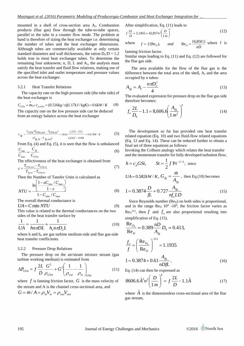
Musinguzi et al. (2016) Parametric Modeling of Producergas-Combustor and Heat Exchanger Integration for …
195 Journal of Energy Challenges and Mechanics ©2016
mounted in a shell of cross-section area As. Combustion
products (flue gas) flow through the tube-to-tube spaces,
parallel to the tube in a counter flow mode. The problem at
hand is therefore of sizing the heat exchanger i.e. determining
the number of tubes and the heat exchanger dimensions.
Although tubes are commercially available at only certain
standard diameters and wall thicknesses, the ration Do/D = 1.2
holds true in most heat exchanger tubes. To determine the
remaining four unknowns; n, D, L and As, the analysis must
satisfy the heat transfer and fluid flow relations, making use of
the specified inlet and outlet temperature and pressure values
across the heat exchanger.
3.2.1 Heat Transfer Relations
The capacity rate on the high pressure side (the tube side) of
the heat exchanger is
KkWkgKkJskgcmC GTmpGTGTm /6.0)/17.1)(/516.0(,
(4)
The capacity rate on the low pressure side can be deduced
from an energy balance across the heat exchanger
KkW
outfgTinfgT
inGTmToutGTmTGTmC
fgC /417.0
8.6192.626,1
523223,1)6.0(
),,(
),,(
(5)
From Eq. (4) and Eq. (5), it is seen that the flow is unbalanced
GTm
fg
C
C
C
C
max
min (6)
The effectiveness of the heat exchanger is obtained from
inGTminfg
inGTmoutGTm
TT
TT
,,
,,
(7)
Then the Number of Tansfer Units is calculated as
maxmin
maxmin
/1
1
/1ln
CC
CC
NTU
(8)
The overall thermal conductance is
NTUCUA min (9)
This value is related to the thermal conductances on the two
sides of the heat transfer surface by
LDnhDLhnUA oo
111 (10)
where h and ho are gas turbine medium-side and flue gas-side
heat transfer coefficients.
3.2.2 Pressure Drop Relations
The pressure drop on the air/steam mixture stream (gas
turbine working medium) is estimated from
GTminoutGTm
GTm GG
D
LfP
112 22
(11)
where f is fanning friction factor, G is the mass velocity of
the stream and A is the channel cross-sectional area, and
outoutinin VVAmG /
After simplification, Eq. (11) leads to 4
2
1857,422455.2
2
m
Dn
D
Lf
(12)
where nD
andff DD
5.850,16Re),(Re where f is
fanning friction factor.
Similar steps leading to Eq. (11) and Eq. (12) are followed for
the flue gas side.
The area available for the flow of the flue gas is the
difference between the total area of the shell, As and the area
occupied by n tubes:
4
2
osfg
DnAA
(13)
The evaluated expression for pressure drop on the flue gas side
therefore becomes:
2
216.606,81.1
2
m
A
D
Lf
fg
h
o (14)
The development so far has provided one heat transfer
related equation (Eq. 10) and two fluid-flow related equations
(Eq. 12 and Eq. 14). These can be reduced further to obtain a
final set of three equations as follows:
Invoking the Colburn analogy which relates the heat transfer
and the momentum transfer for fully developed turbulent flow;
3/2Pr2
1, fStGStch p ; since
,/582.0 KkWUAfg
fgA
mG
, then Eq.(10) becomes
LDnf
A
fL
D
o
fg727.03874.01 (15)
Since Reynolds number (ReD) on both sides is proportional,
and in the range ReD 104 -106, the friction factor varies as
ReD-0.2, then f and of are also proportional resulting into
simplification of Eq. (15).
1935.1Re
Re
,413.0389.0Re
Re
2.0
D
Do
h
fgD
D
h
h
f
f
DA
nD
nDfL
Afg61.03874.01 , (16)
Eq. (14) can then be expressed as
AD
Lf
m
DnA ˆ1.1
2
1ˆ6.8606
4
23
(17)
where A is the dimensionless cross-sectional area of the flue
gas stream,
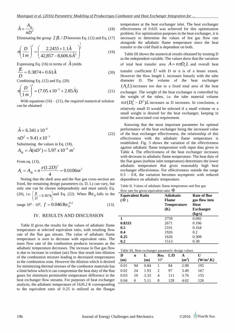
Musinguzi et al. (2016) Parametric Modeling of Producergas-Combustor and Heat Exchanger Integration for …
196 Journal of Energy Challenges and Mechanics ©2016
2ˆ
nD
AA
fg (18)
Eliminating the group DfL /2 between Eq. (12) and Eq. (17)
2
1
3
2
ˆ6.606,8857,42
ˆ1.12455.2
1
A
A
m
Dn (19)
Expressing Eq. (16) in terms of A yields
AD
fL ˆ61.03874.0 (20)
Combining Eq. (12) and Eq. (20)
)ˆ85.21005.7(1
5
2
Axm
Dn
(21)
With equations (16) – (21), the required numerical solution
can be obtained
32
6
1041.9
10341.6ˆ
xnD
xA (22)
Substituting the values in Eq. (18), 282 1097.5)(ˆ mxnDAAfg
From eq. (13),
22
0106.04
)2.1(m
DnAA fgs
Noting that the shell area and the flue gas cross-section are
fixed, the remaining design parameters (n, D, L) can vary, but
only one can be chosen independently and must satisfy Eq.
(20), i.e.
3874.0
D
fL and Eq. (22). When DRe falls in the
range 104 – 106, 2.0Re046.0 Df
[13].
IV. RESULTS AND DISCUSSION
Table II gives the results for the values of adiabatic flame
temperature at selected equivalent ratio, with resulting flow
rate of the flue gas stream. The value of adiabatic flame
temperature is seen to decrease with equivalent ratio. The
mass flow rate of the combustion products increases as the
adiabatic temperature decreases. The increase in flue gas flow
is due to increase in oxidant (air) flow that result into dilution
of the combustion mixture leading to decreased temperatures
in the combustion zone. However the dilution which is desired
for minimizing thermal stresses of the combustor materials has
a limit below which it can compromise the heat duty of the flue
gases for minimum permissible temperature difference in the
heat exchanger flow streams. For purposes of heat exchanger
analysis, the adiabatic temperature of 1626.2 K corresponding
to the equivalent ratio of 0.25 is utilized as the fluegas
temperature at the heat exchanger inlet. The heat exchanger
effectiveness of 0.635 was achieved for this optimization
problem. For optimization purposes in the heat exchanger, it is
necessary to determine the values of hot gas flow rate
alongside the adiabatic flame temperature since the heat
transfer to the cold fluid is dependent on both.
Table III shows the numerical results obtained by treating D
as the independent variable. The values show that the variation
of total heat transfer area LDnA o and overall heat
transfer coefficient U with D or n is of a lesser extent.
However the flow length L increases linearly with the tube
diameter D. The volume of the heat exchanger
)( LAs increases too due to a fixed total area of the heat
exchanger. The weight of the heat exchanger is controlled by
the weight of the tubes, i.e. the tube material volume
LDDn )( 22
0 increases as D increases. In conclusion, a
relatively small D would be selected if a small volume or a
small weight is desired for the heat exchanger, keeping in
mind the associated cost requirement.
Knowing that the most important parameter for optimal
performance of the heat exchanger being the increased value
of the heat exchanger effectiveness, the relationship of this
effectiveness with the adiabatic flame temperature is
established. Fig. 3 shows the variation of the effectiveness
against adiabatic flame temperature with input data given in
Table 4. The effectiveness of the heat exchanger increases
with decrease in adiabatic flame temperature. The heat duty of
the flue gases (turbine inlet temperature) determines the lower
adiabatic temperature that gives reasonably high heat
exchanger effectiveness. For effectiveness outside the range
0.3 – 0.8, the variation becomes asymptotic with reduced
dependence on adiabatic temperature.
Table II, Values of adiabatic flame temperature and flue gas
flow rate for given equivalent ratio
Equivalent Ratio
( )
Adiabatic
Flame
Temperature
(K)
Rate of flue
gas flow into
Heat
Exchanger
(kg/s)
1 2759 0.092
0.8333 2671 0.106
0.5 2101 0.164
0.4 1926 0.2
0.25
0.2
1626
1513
0.308
0.38
Table III, Heat exchanger parametric design values
D
(m)
n L
(m)
ReD
105
L/D A
(m2)
U
(W/m2.K)
0.01 94 0.84 1 84 2.98 195
0.02 24 1.93 2 97 3.49 167
0.03 10 3.33 4 111 3.76 155
0.04 6 5.11 8 128 4.62 126
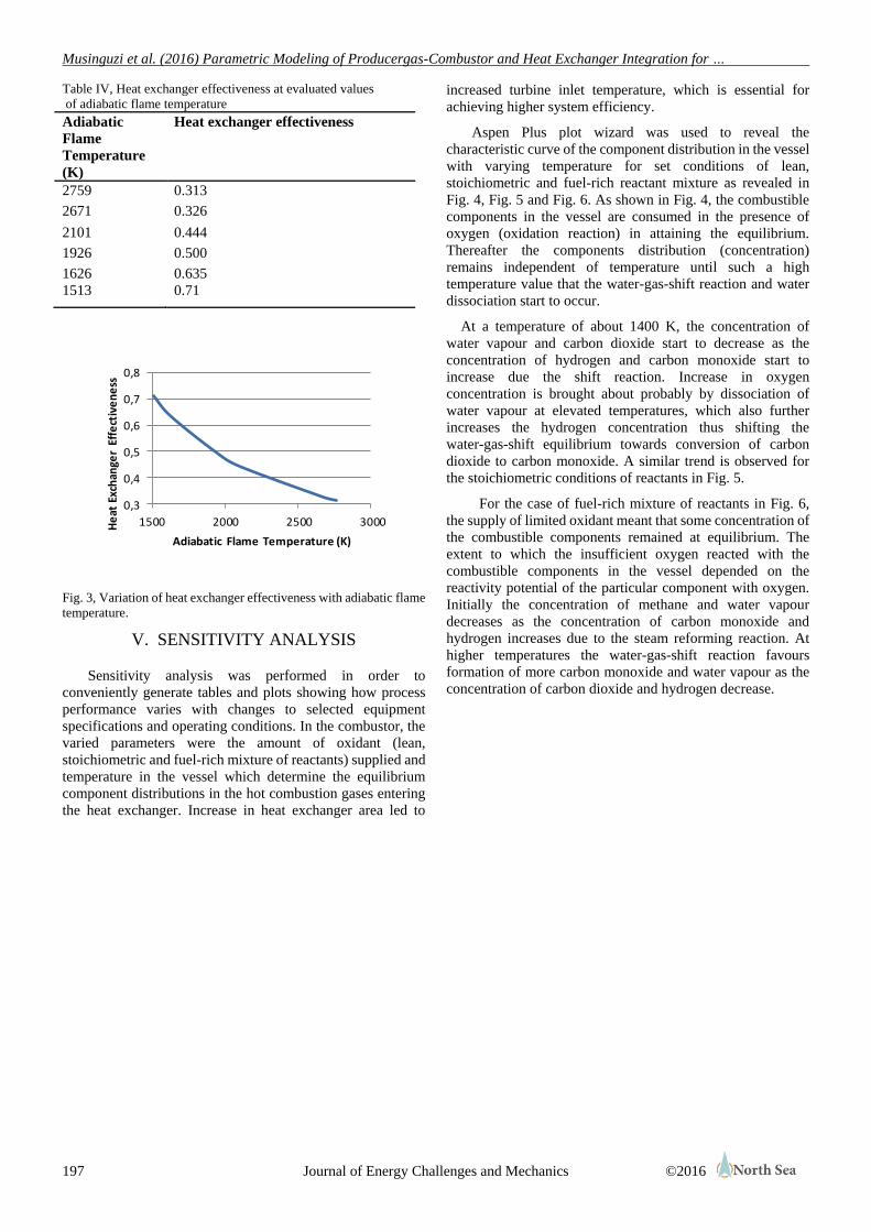
Musinguzi et al. (2016) Parametric Modeling of Producergas-Combustor and Heat Exchanger Integration for …
197 Journal of Energy Challenges and Mechanics ©2016
Table IV, Heat exchanger effectiveness at evaluated values
of adiabatic flame temperature
Adiabatic
Flame
Temperature
(K)
Heat exchanger effectiveness
2759 0.313
2671 0.326
2101 0.444
1926 0.500
1626
1513
0.635
0.71
0,3
0,4
0,5
0,6
0,7
0,8
1500 2000 2500 3000He
at E
xch
ange
r Ef
fect
ive
ne
ss
Adiabatic Flame Temperature (K)
Fig. 3, Variation of heat exchanger effectiveness with adiabatic flame
temperature.
V. SENSITIVITY ANALYSIS
Sensitivity analysis was performed in order to
conveniently generate tables and plots showing how process
performance varies with changes to selected equipment
specifications and operating conditions. In the combustor, the
varied parameters were the amount of oxidant (lean,
stoichiometric and fuel-rich mixture of reactants) supplied and
temperature in the vessel which determine the equilibrium
component distributions in the hot combustion gases entering
the heat exchanger. Increase in heat exchanger area led to
increased turbine inlet temperature, which is essential for
achieving higher system efficiency.
Aspen Plus plot wizard was used to reveal the
characteristic curve of the component distribution in the vessel
with varying temperature for set conditions of lean,
stoichiometric and fuel-rich reactant mixture as revealed in
Fig. 4, Fig. 5 and Fig. 6. As shown in Fig. 4, the combustible
components in the vessel are consumed in the presence of
oxygen (oxidation reaction) in attaining the equilibrium.
Thereafter the components distribution (concentration)
remains independent of temperature until such a high
temperature value that the water-gas-shift reaction and water
dissociation start to occur.
At a temperature of about 1400 K, the concentration of
water vapour and carbon dioxide start to decrease as the
concentration of hydrogen and carbon monoxide start to
increase due the shift reaction. Increase in oxygen
concentration is brought about probably by dissociation of
water vapour at elevated temperatures, which also further
increases the hydrogen concentration thus shifting the
water-gas-shift equilibrium towards conversion of carbon
dioxide to carbon monoxide. A similar trend is observed for
the stoichiometric conditions of reactants in Fig. 5.
For the case of fuel-rich mixture of reactants in Fig. 6,
the supply of limited oxidant meant that some concentration of
the combustible components remained at equilibrium. The
extent to which the insufficient oxygen reacted with the
combustible components in the vessel depended on the
reactivity potential of the particular component with oxygen.
Initially the concentration of methane and water vapour
decreases as the concentration of carbon monoxide and
hydrogen increases due to the steam reforming reaction. At
higher temperatures the water-gas-shift reaction favours
formation of more carbon monoxide and water vapour as the
concentration of carbon dioxide and hydrogen decrease.
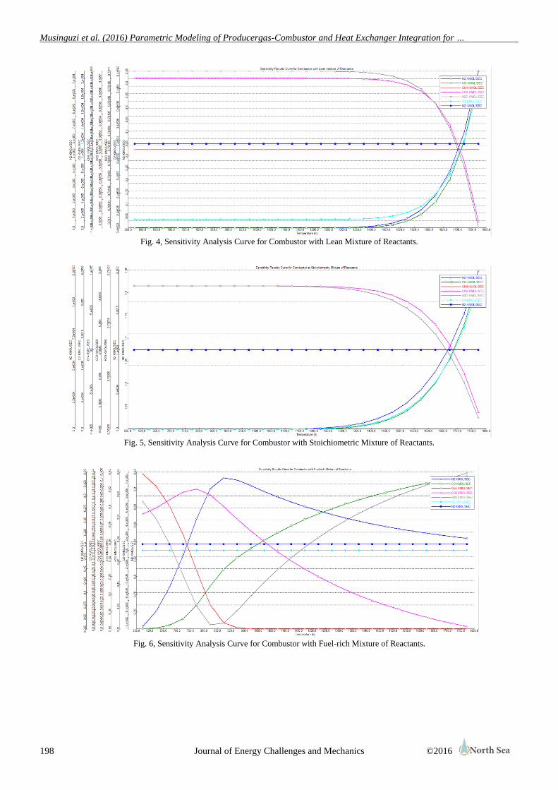
Musinguzi et al. (2016) Parametric Modeling of Producergas-Combustor and Heat Exchanger Integration for …
198 Journal of Energy Challenges and Mechanics ©2016
Fig. 4, Sensitivity Analysis Curve for Combustor with Lean Mixture of Reactants.
Fig. 5, Sensitivity Analysis Curve for Combustor with Stoichiometric Mixture of Reactants.
Fig. 6, Sensitivity Analysis Curve for Combustor with Fuel-rich Mixture of Reactants.

Musinguzi et al. (2016) Parametric Modeling of Producergas-Combustor and Heat Exchanger Integration for …
199 Journal of Energy Challenges and Mechanics ©2016
VI. CONCLUSION
The authors have carried out parametric modeling of the
system to reveal the relationship of different parameters in the
system in order to achieve the desired output of heat
transferred to the turbine working fluid. The turbine inlet
parameters are specified by the design model chosen and thus
the turbine inlet temperature is set at 950oC. Though attempts
to have the highest possible practical value of the key
parameter of heat exchanger effectiveness and thus high heat
transfer to the turbine medium were made, the author’s cannot
comfortably conclude that this is a generally accepted optimal
value but rather a near optimal one.
The value of adiabatic flame temperature is seen to decrease
with equivalent ratio. The mass flow rate of the combustion
products increases as the adiabatic temperature decreases. The
increase in flue gas flow is due to increase in oxidant (air) flow
that results into dilution of the combustion mixture leading to
decreased temperatures in the combustion zone. However the
dilution which is desired for minimizing thermal stresses of
the combustor materials has a limit below which it can
compromise the heat duty of the flue gases for minimum
permissible temperature difference in the heat exchanger flow
streams. For purposes of heat exchanger analysis, the adiabatic
temperature of 1626.2 K corresponding to the equivalent ratio
of 0.25 is utilized as the fluegas temperature at the heat
exchanger inlet. For optimization purposes in the heat
exchanger, it is necessary to determine the values of hot gas
flow rate alongside the adiabatic flame temperature since the
heat transfer to the cold fluid is dependent on both. The
stoichiometry of the combustion products determines the
equilibrium concentrations and parameters of the combustion
gas as revealed by the Aspen Plot wizard curves.
The analysis of combustion of the wood gas has revealed
that high temperatures can be achieved in the combustor
region. The heat exchanger and combustor integration process
analysis has also shown good performance with the flue gases
from combustion of producer gas providing sufficient thermal
energy needed to raise the turbine working fluid to the
required turbine inlet temperature. The analysis of the heat
exchanger has provided parameters essential for decision
making on the sizing of the heat exchanger. The practical
value added was revealing the parameters needed in the design
specification of the heat exchanger suitable for the heat duty of
a typical 100kWe externally fired micro gas turbine based on
gasification of biomass and subsequent producer gas
combustion. The heat exchanger effectiveness of 0.635 was
achieved in this parametric study. Due to high temperature
involved in the process, materials that can withstand high
temperature stresses have to be chosen.
The choice of a suitable Gasification system is driven by
the need and local conditions at the target end user, keeping in
mind that the system integration should have a good balance of
being most efficient, cost effective, reliable, least polluting,
sustainable in the long run and socially beneficial. Innovative
systems which take into consideration the local conditions
such as biomass fuel characteristics have shown great success
in other countries. Therefore issues of unpredictable fuel
behavior during thermochemical conversion, unreliable
operating conditions, and low overall efficiency need to be
addressed through continued research to make the gasification
technology more attractive.
ACKNOWLEDGEMENT
This work was funded by the Norwegian Agency for
Development Cooperation (NORAD) through the Energy and
Petroleum (EnPe) Project, as part of the collaboration between
The Norwegian University of Science and Technology
(NTNU), Trondheim, Norway and Makerere University,
Kampala, Uganda.

Musinguzi et al. (2016) Parametric Modeling of Producergas-Combustor and Heat Exchanger Integration for …
200 Journal of Energy Challenges and Mechanics ©2016
REFERENCES
[1] D. Maraver, A. Sin, J. Royo, F. Sebastián. “Assessment
of CCHP systems based on biomass combustion for
small-scale applications through a review of the
technology and analysis of energy efficiency
parameters”, Applied Energy, 102, pp. 1303-1313,
2013.
[2] D. Leilei, L. Hao, R. Saffa. “Development of small-scale
and micro-scale biomass-fuelled CHP systems –
A literature review”, Applied Thermal Engineering, 29,
pp. 2119-2126, 2008.
[3] J.H. Juan, A.A. Guadalupe, B. Antonio. “Gasification of
biomass wastes in an entrained flow gasifier:
Effect of the particle size and the residence time”, Fuel
Processing Technology, 91, pp. 681-692, 2010.
[4] M. Puig-Arnavat, C.B. Joan, C. Alberto. “Review and
Analysis of Biomass Gasification models”,
Renewable and Sustainable Energy Reviews,14, pp.
2841-2851, 2010.
[5] P.A. Pilavachi. “Power generation with gas turbine
systems and combined heat and power”, Applied
Thermal Engineering, 20, pp. 1421-1429, 2000.
[6] A.M. Bassily. “Enhancing the efficiency and power of
the triple-pressure reheat combined cycle by means
of gas reheat, gas recuperation, and reduction of the
irreversibility in the heat recovery steam generator”,
Applied Energy, 85, pp. 1141-1162, 2008.
[7] M. Kautz, H. Ulf. “The externally-fired gas-turbine
(EFGT-Cycle) for decentralized use of biomass”,
Applied Energy , 84, pp. 795-805, 2007.
[8] M. Gaderer, G. Gallmetzer, H. Spliethoff. “Biomass fired
hot air gas turbine with fluidized bed
combustion”, Applied Thermal Engineering, 30, pp.
1594-1600, 2010.
[9] A. Sommers, Q. Wang, X. Han, C. T'Joen, Y. Park, A.
Jacobi. “Ceramics and ceramic matrix composites
for heat exchangers in advanced thermal systems—A
review”, Applied Thermal Engineering, 30, pp. 2137-
2152, 2010.
[10] F. Delattin, B. Svend, J.D. Ruyck. “Effects of steam
injection on microturbine efficiency and
performance”, Energy , 33, pp. 241-247, 2007.
[11] W.B. Musinguzi, M.A.E. Okure, L. Wang, A. Sebbit, T.
Løvås. “Thermal characterization of Uganda's
Acacia hockii, Combretum molle, Eucalyptus grandis
and Terminalia glaucescens for gasification”,
Biomass and Bioenergy, 46, pp. 402-408, 2012.
[12] W.B. Musinguzi, M.A.E. Okure, A. Sebbit, T. Løvås,
I.P. Da Silva. “Thermodynamic Modeling of
Allothermal Steam Gasification in a Downdraft
Fixed-bed Gasifier”, Advanced Materials Research,
875- 877, pp. 1782 -1793, 2014.
[13] G. Schuster, G, Löffler, K. Weigl, H. Hofbauer.
“Biomass steam gasification – an extensive
parametric modeling study”, Bioresource
Technology, 77, pp. 71-79, 2001.
[14] U. Kentaro, Y. Kouichi, N. Tomoaki, Y. Kunio.
“High temperature steam-only gasification of woody biomass”, Applied Energy, 87, pp. 791-798, 2009.
[15] D. Chiaramonti, R. Giovanni, M. Francesco.
“Preliminary design and economic analysis of a biomass
fed micro-gas turbine plant for decentralized energy
generation in Tuscany,” Paper GT2004-53546, The
American Society of Mechanical Engineers (ASME)
Turbo Expo proceedings, Vienna, Austria, June 14-
17,2004. [16] C. Daniele, D. Paolo, C. Giorgio. “Performance
evaluation of small size externally fired gas turbine (EFGT) power plants integrated with direct biomass
dryers”, Energy , 31, pp. 1459-1471, 2005.
[17] T. Lieuwen, V. McDonell, D. Santavicca, T.
Sattelmayer. “Burner Development and Operability
Issues Associated with Steady Flowing Syngas Fired
Combustors”, Combustion Science Technology, 180,
pp.1169-1192, 2008.
[18] E.L. Keating. Applied Combustion. New York: Taylor
& Francis Group, 2007.
[19] A. Bejan, G. Tsatsaronis, M. Moran. Thermal Design
and Optimization. New York: John Wiley and Sons
Inc., 1996.

ISSN 2056-9386
Volume 3 (2016) issue 4, article 5
201 ©2016
Behavior, cutting property and environmental load of
machine tool in mist of strong alkaline water
机床在强碱性水雾中的行为,切割性能与环境负荷
Ikuo Tanabe1*
1Department of Mechanical Engineering, Nagaoka University of Technology, 1603-1 Kamitomioka Nagaoka Niigata, 940-2188
JAPAN
Accepted for publication on 11th August 2016
Abstract - In the 21st century, as it is important to produce
products with care for protecting the earth, a producer must be
careful to conserve energy, save resources and reduce waste which
pollutes environment. Further, in case of a machine tool, much
lubricating oil was used for smooth drive, electrical energy of
forced cooling was used for high accuracy and much cutting oil
was also used for lubrication and cooling. This is a large problem
for protecting the earth. Therefore, the behavior of a machine tool
in the mist of strong alkaline water was investigated and evaluated.
Properties of strong alkaline water were firstly investigated for
alkali-proof, corrosion and safety of health. Then the bench lathe
was remodeled in the vessel with the mist of strong alkaline water
(pH12.5), thermal deformation between the spindle and the tool
post was measured for evaluation of accuracy. And cutting using
CNC milling machine in the vessel with the mist of strong alkaline
water was performed for investigating the effect of water
evaporation in the strong alkaline water. It is concluded from the
results that; (1) Alkali-proof regarding several elements of a
machine tool and safety of health were cleared in the experiment,
(2) The forced cooling using mist of strong alkaline water had a
very strong influence. Thus, it could be said that the thermal
deformation of structure can be effectively cooled by using a mist of
strong alkaline water, (3) Thermal deformation of the bench lathe
was very small despite no-forced cooling, (4) Accuracy of the
machine tool was very good and the tool life was very long despite
no-cutting oil, (5) Mist of strong alkaline was eco-friendly.
Keywords - forced cooling, machine tool, high accuracy, strong
alkaline water, cutting, eco-Friendly
I. INTRODUCTION
Since the beginning of the 21st century, the importance to
manufacture products in an environmentally-conscious [1]
way has been highlighted. In this regard, manufacturers not
only need to conserve energy, but they also need to scrutinize
in order to save resources and reduce environmentally-harmful
pollutants. Nowadays, there are many researches related to the
environmental impact of men [2], as well as countermeasures
to reduce it [3]; however, these are still insufficient.
Particularly, in the field of manufacturing, most machine tools
highly depend on cutting and cooling oils to achieve the high
accuracy. This represents a large environmental problem,
since in most cases the cutting and cooling oils are misused,
introduced into the environment and generate undesired
pollution [4]. Consequently, the importance of developing
new manufacturing ideas that consider parameters such as
high accuracy, high quality and a low environmental impact
had been underlined. Hence, manufacturers will be in the need
of daring plans, unique ideas and new technologies [5].
Therefore, even though the cutting concept of this research
is ecology, it also included other concepts related to the
industrial sector. Among these are: suitable cost of a machine
tool, low running and maintenance cost with high precision
machining. Thus, this study is to achieve the application of the
ecology and multiple industrial sector-related concepts, in
conjunction with the advances of production engineering
technology. For instance, regarding machine tool technology,
while restraint of the thermal deformation on a machine tool
was attempted to achieve high accuracy and quality, it was at
the expense of using costly equipment and a large quantity of
electrical energy. Even then, those countermeasures taken
were not enough to satisfy these parameters [6].
Therefore, behavior of a machine tool in mist of strong
alkaline water were investigated and evaluated. Properties of
strong alkaline water were firstly investigated for alkali-proof,
corrosion and safety of health. Then the bench lathe was
remodeled in the vessel with mist of strong alkaline water
(pH12.5), thermal deformation between the spindle and the
tool post was measured for evaluation of accuracy. And
cutting using CNC milling machine in the vessel with mist of
strong alkaline water was performed for investigating the
effect of water evaporation in the strong alkaline water.

Tanabe (2016) Behavior, cutting property and environmental load of machine tool in mist of strong alkaline water
202 Journal of Energy Challenges and Mechanics ©2016
II. THE CORROSION RESISTANCE OF MATERIALS IN
STRONG ALKALINE WATER
The strong alkali water with pH value above 12.5 has high
interfacial permeability, dissolving, emulsification, and
separation properties. For these properties, it is well using for
washing, sterilization, corruption prevention. Moreover, when
strong alkaline water is kept long time in the air, it lost alkali
property and become normal water of pH 7.0. This fact also
regarded as very excellent for using it as cleaning agent with
improved environmental protection.
In this section, the reactions of the various materials in
strong alkaline water are tested. The specification of the
device for making alkaline water is shown in Table 1. It is
small and compact for making alkaline water of pH12.5. Fig. 1
shows the measurement results of pH values for keeping 10 L
of strong alkaline water (pH12.5) in three containers (diameter
φ25 mm, height 230 mm) and kept exposed to air for 2
months, in three different environment conditions. These
conditions are different temperatures of 20oC, 40
oC and 12
oC
with humidity 60% respectively. It is confirmed that the
change in pH value even for the most decreasing condition
with 40 oC is just drop from pH 12.5 to pH12.0 during two
months experiment. In the practical application of this method,
there exist natural evaporation and evaporation due to
generated cutting heat and it is necessary to fill up alkaline
water to keep maintain the amount and pH value of water.
However, from this experiment, it can be considered that this
decreasing rate of pH value is quite enough to endure for the
practical application of proposed method.
In the corrosion engineering, logarithmic value of metal ion
concentration lesser than (-6) could not be corroded at
equilibrium state. Here, according to the corrosion
characteristic [7] of strong alkaline water, steel could not
corrode in the alkaline water above pH10. Similarly, Nickel in
the Nickel based alloys shows no chemical reaction in the
range of pH8.5~pH13.0. Moreover, titanium alloys also shows
no effect under pH13.0 range. From these facts, it can be
considered that it is possible to operate underwater metal
AAAAA
cutting processing of Titanium and Nickel alloy materials for
compulsory water evaporative cooling with using the optimum
range of pH values between pH10.0~pH13.0. The corrosion
characteristics of these materials are also confirmed by
experiment.
In the experiment, the tested materials are steel, titanium
alloy, nickel alloy and those being used well in industries such
as, copper, aluminum, brass and carbide (tool material) as
shown in Table 3.
These materials are put in the test tubes containing water
with three pH values, pH7.0, pH10.0, pH12.5 and keep in a
room with constant temperature of 20±1 oC and 60% moisture
for two months (see Table 2). The pH value is made to kept
constant by changing alkaline water once per week.
The result of the experiment regarding to alkali resistance of
the materials are shown in Table 3. The results shown there
was no corrosion exhibit for the tested materials placing inside
strong alkaline water for two months except aluminum. From
this result, it was confirmed that the underwater cutting
process for titanium alloys and nickel alloys can be applicable
for compulsory tool cooling effect with the exception of
aluminum. For cutting aluminum, it is necessary to take
precaution and improvement as it is corroded in strong
alkaline water. For the case of copper and brass, there occurred
change in color.
Table 2 Materials and conditions used in corrosion test
Medium in the vessel Strong alkaline water (pH 12.5)
Ambient conditions Room temp.: 20±1℃, Humidity: 60%
Period Two months
Table 1 Specification of the system for making strong alkaline water and safty of health for strong alkaline water
Method of generation Closed generation type Assistant material Potassium carbonate
Value of pH pH 12.5 Safety
of
health
Smell ○ Odourless
Quantity of generation 10 ℓ/h Touch △ Wear gloves & glasses
Voltage & Power 100 V & 300W Breath △ Wear mask
Size 495W×430D×1100H Drink ×
○:No problem △:Avoid ×:Prohibition
Fig. 1 Variation of pH values in different temperatures
20℃
40℃
11.9
12.1
12.3
12.5
12.7
Measuring time days
Chan
ge
of
acid
ity
pH
0 10 20 30 40 50 60
12℃
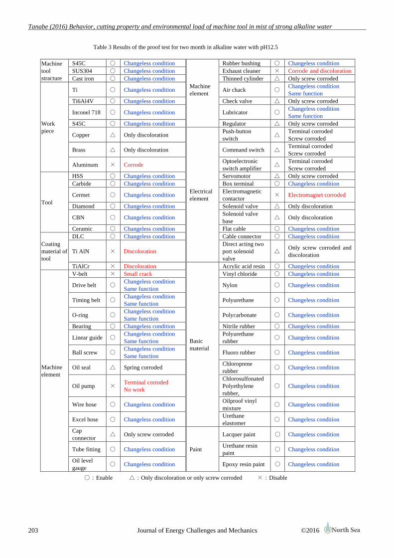
Tanabe (2016) Behavior, cutting property and environmental load of machine tool in mist of strong alkaline water
203 Journal of Energy Challenges and Mechanics ©2016
Table 3 Results of the proof test for two month in alkaline water with pH12.5
Machine
tool
stracture
S45C ○ Changeless condition
Machine
element
Rubber bushing ○ Changeless condition
SUS304 ○ Changeless condition Exhaust cleaner × Corrode and discoloration
Cast iron ○ Changeless condition Thinned cylinder △ Only screw corroded
Work
piece
Ti ○ Changeless condition Air chack ○ Changeless condition
Same function
Ti6Al4V ○ Changeless condition Check valve △ Only screw corroded
Inconel 718 ○ Changeless condition Lubricator ○ Changeless condition
Same function
S45C ○ Changeless condition Regulator △ Only screw corroded
Copper △ Only discoloration
Electrical
element
Push-button
switch △
Terminal corroded
Screw corroded
Brass △ Only discoloration Command switch △ Terminal corroded
Screw corroded
Aluminum × Corrode Optoelectronic
switch amplifier △
Terminal corroded
Screw corroded
Tool
HSS ○ Changeless condition Servomotor △ Only screw corroded
Carbide ○ Changeless condition Box terminal ○ Changeless condition
Cermet ○ Changeless condition Electromagnetic
contactor × Electromagnet corroded
Diamond ○ Changeless condition Solenoid valve △ Only discoloration
CBN ○ Changeless condition Solenoid valve
base △ Only discoloration
Ceramic ○ Changeless condition Flat cable ○ Changeless condition
Coating
material of
tool
DLC ○ Changeless condition Cable connector ○ Changeless condition
Ti AlN × Discoloration
Direct acting two
port solenoid
valve
△ Only screw corroded and
discoloration
TiAlCr × Discoloration
Basic
material
Acrylic acid resin ○ Changeless condition
Machine
element
V-belt × Small crack Vinyl chloride ○ Changeless condition
Drive belt ○ Changeless condition
Same function Nylon ○ Changeless condition
Timing belt ○ Changeless condition
Same function Polyurethane ○ Changeless condition
O-ring ○ Changeless condition
Same function Polycarbonate ○ Changeless condition
Bearing ○ Changeless condition Nitrile rubber ○ Changeless condition
Linear guide ○ Changeless condition
Same function
Polyurethane
rubber ○ Changeless condition
Ball screw ○ Changeless condition
Same function Fluoro rubber ○ Changeless condition
Oil seal △ Spring corroded Chloroprene
rubber ○ Changeless condition
Oil pump × Terminal corroded
No work
Chlorosulfonated
Polyethylene
rubber,
○ Changeless condition
Wire hose ○ Changeless condition Oilproof vinyl
mixture ○ Changeless condition
Excel hose ○ Changeless condition Urethane
elastomer ○ Changeless condition
Cap
connector △ Only screw corroded
Paint
Lacquer paint ○ Changeless condition
Tube fitting ○ Changeless condition Urethane resin
paint ○ Changeless condition
Oil level
gauge ○ Changeless condition Epoxy resin paint ○ Changeless condition
○:Enable △:Only discoloration or only screw corroded ×:Disable
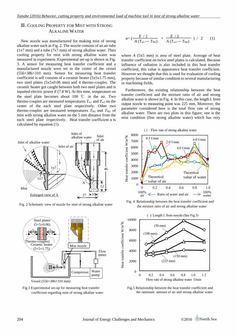
Tanabe (2016) Behavior, cutting property and environmental load of machine tool in mist of strong alkaline water
204 Journal of Energy Challenges and Mechanics ©2016
Ⅲ. COOLING PROPERTY FOR MIST WITH STRONG
ALKALINE WATER
New nozzle was manufactured for making mist of strong
alkaline water such as Fig. 2. The nozzle consists of an air tube
(1x7 mm) and a tube (7x7 mm) of strong alkaline water. Then
cooling property for mist with strong alkaline water was
measured in experiment. Experimental set-up is shown in Fig.
3. A sensor for measuring heat transfer coefficient and a
manufactured nozzle were set in the center of the vessel
(556×386×310 mm). Sensor for measuring heat transfer
coefficient is self consists of a ceramic heater (5x5x1.75 mm),
two steel plates (5x5x0.06 mm) and 4 thermo-couples. The
ceramic heater got caught between both two steel plates and is
inputted electric power E (7.8 W). At this time, temperature on
the steel plate becomes about 100 ℃ in the air. Two
thermo-couples are measured temperatures Tw1 and Tw2 on the
center of the each steel plate respectively. Other two
thermo-couples are measured temperatures TM1 and TM2 of
mist with strong alkaline water on the 5 mm distance from the
each steel plate respectively. Heat transfer coefficient α is
calculated by equation (1).
(1)
where A (5x5 mm) is area of steel plate. Average of heat
transfer coefficient on twice steel plates is calculated. Because
influence of radiation is also included in this heat transfer
coefficient, this value is appearance heat transfer coefficient.
However we thought that this is used for evaluation of cooling
property because of similar condition to several manufacturing
or machining fields.
Furthermore, the existing relationship between the heat
transfer coefficient and the mixture ratio of air and strong
alkaline water is shown in Fig. 4. In this case, the length L from
output nozzle to measuring point was 225 mm. Moreover, the
parameter considered here is the total flow rate of strong
alkaline water. There are two plots in this figure; one is the
mist condition (fine strong alkaline water) which has very
AAA
Fig.3 Experimental set-up for measuring heat transfer
coefficient regarding mist of strong alkaline water
Flow meter
Vessel (556×386×310 mm)
L
Mist nozzle
Water pump
Compressor
Steel plates
(5×5×0.06)
Ceramic heater
(5×5×1.75)
5 5
Thermo-couples)
α= ( + ) / 2
E / 2 E / 2
A (Tw1 ― TM1) A (Tw2 ― TM2)
Fig. 2 Schematic view of nozzle for mist of strong alkaline water
Enlarged view of A
Inlet of alkaline water
Inlet of air
Mist
1x7
1x7
A
Inlet of air
Inlet of alkaline water
46
12
10 27
.5
( ):Flow rate of strong alkaline water
0.5 ℓ/min
2.0 ℓ/min
4.0 ℓ/min
6.0 ℓ/min
Theoretical
value of air
Theoretical
value of water
8000
7000
6000
5000
4000
3000
2000
1000
0
Hea
t tr
ansf
er c
oef
fici
ent
W/m
2K
Fig. 4 Relationship between the heat transfer coefficient and
the mixture ratio of air and strong alkaline water
0 0.2 0.4 0.6 0.8 1.0 Ratio of water and air
100% air
100% water
( ): Length L from noozle (See Fig.3)
Fig.5 Relationship between the heat transfer coefficient and
the optimum amount of air and strong alkaline water
(50 mm)
(100 mm)
(150 mm)
(225 mm)
10000
8000
6000
4000
2000
0
Hea
t tr
ansf
er c
oef
fici
ent
W/m
2K
0 0.2 0.4 0.6 0.8 1.0 1.2
Flow rate of strong alkaline water ℓ/min
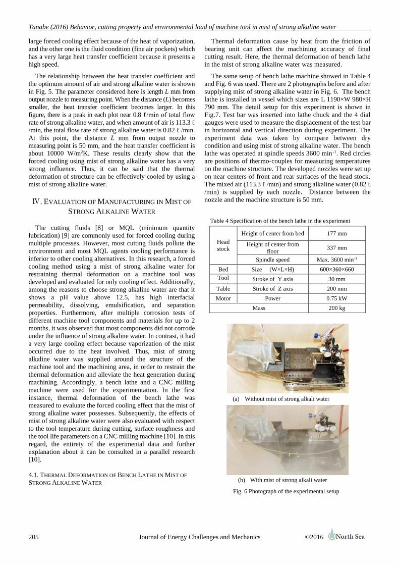
Tanabe (2016) Behavior, cutting property and environmental load of machine tool in mist of strong alkaline water
205 Journal of Energy Challenges and Mechanics ©2016
large forced cooling effect because of the heat of vaporization,
and the other one is the fluid condition (fine air pockets) which
has a very large heat transfer coefficient because it presents a
high speed.
The relationship between the heat transfer coefficient and
the optimum amount of air and strong alkaline water is shown
in Fig. 5. The parameter considered here is length L mm from
output nozzle to measuring point. When the distance (L) becomes
smaller, the heat transfer coefficient becomes larger. In this
figure, there is a peak in each plot near 0.8 ℓ/min of total flow
rate of strong alkaline water, and when amount of air is 113.3 ℓ
/min, the total flow rate of strong alkaline water is 0.82 ℓ /min.
At this point, the distance L mm from output nozzle to
measuring point is 50 mm, and the heat transfer coefficient is
about 10000 W/m2K. These results clearly show that the
forced cooling using mist of strong alkaline water has a very
strong influence. Thus, it can be said that the thermal
deformation of structure can be effectively cooled by using a
mist of strong alkaline water.
Ⅳ. EVALUATION OF MANUFACTURING IN MIST OF
STRONG ALKALINE WATER
The cutting fluids [8] or MQL (minimum quantity
lubrication) [9] are commonly used for forced cooling during
multiple processes. However, most cutting fluids pollute the
environment and most MQL agents cooling performance is
inferior to other cooling alternatives. In this research, a forced
cooling method using a mist of strong alkaline water for
restraining thermal deformation on a machine tool was
developed and evaluated for only cooling effect. Additionally,
among the reasons to choose strong alkaline water are that it
shows a pH value above 12.5, has high interfacial
permeability, dissolving, emulsification, and separation
properties. Furthermore, after multiple corrosion tests of
different machine tool components and materials for up to 2
months, it was observed that most components did not corrode
under the influence of strong alkaline water. In contrast, it had
a very large cooling effect because vaporization of the mist
occurred due to the heat involved. Thus, mist of strong
alkaline water was supplied around the structure of the
machine tool and the machining area, in order to restrain the
thermal deformation and alleviate the heat generation during
machining. Accordingly, a bench lathe and a CNC milling
machine were used for the experimentation. In the first
instance, thermal deformation of the bench lathe was
measured to evaluate the forced cooling effect that the mist of
strong alkaline water possesses. Subsequently, the effects of
mist of strong alkaline water were also evaluated with respect
to the tool temperature during cutting, surface roughness and
the tool life parameters on a CNC milling machine [10]. In this
regard, the entirety of the experimental data and further
explanation about it can be consulted in a parallel research
[10].
4.1. THERMAL DEFORMATION OF BENCH LATHE IN MIST OF
STRONG ALKALINE WATER
Thermal deformation cause by heat from the friction of
bearing unit can affect the machining accuracy of final
cutting result. Here, the thermal deformation of bench lathe
in the mist of strong alkaline water was measured.
The same setup of bench lathe machine showed in Table 4
and Fig. 6 was used. There are 2 photographs before and after
supplying mist of strong alkaline water in Fig. 6. The bench
lathe is installed in vessel which sizes are L 1190×W 980×H
790 mm. The detail setup for this experiment is shown in
Fig.7. Test bar was inserted into lathe chuck and the 4 dial
gauges were used to measure the displacement of the test bar
in horizontal and vertical direction during experiment. The
experiment data was taken by compare between dry
condition and using mist of strong alkaline water. The bench
lathe was operated at spindle speeds 3600 min -1. Red circles
are positions of thermo-couples for measuring temperatures
on the machine structure. The developed nozzles were set up
on near centers of front and rear surfaces of the head stock.
The mixed air (113.3 ℓ /min) and strong alkaline water (0.82 ℓ
/min) is supplied by each nozzle. Distance between the
nozzle and the machine structure is 50 mm.
Table 4 Specification of the bench lathe in the experiment
Head
stock
Height of center from bed 177 mm
Height of center from
floor 337 mm
Spindle speed Max. 3600 min-1
Bed Size (W×L×H) 600×360×660
Tool
post Stroke of Y axis 30 mm
Table Stroke of Z axis 200 mm
Motor Power 0.75 kW
Mass 200 kg
(b) With mist of strong alkali water
Fig. 6 Photograph of the experimental setup
(a) Without mist of strong alkali water
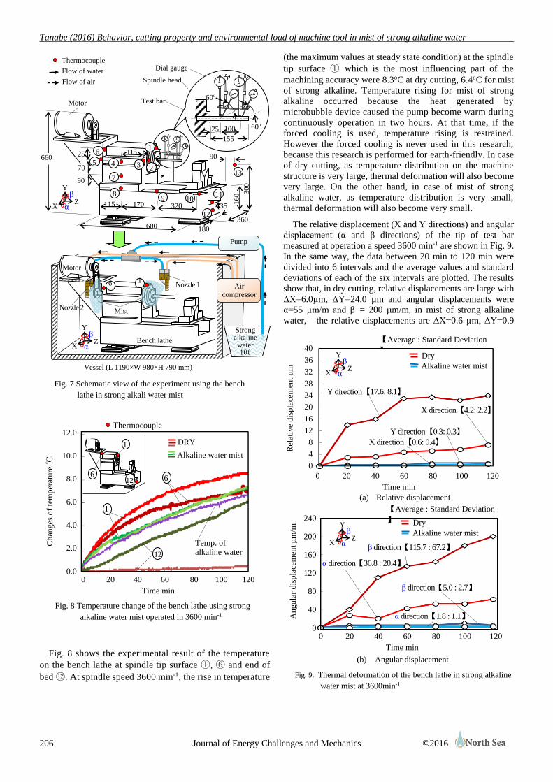
Tanabe (2016) Behavior, cutting property and environmental load of machine tool in mist of strong alkaline water
206 Journal of Energy Challenges and Mechanics ©2016
Fig. 8 shows the experimental result of the temperature
on the bench lathe at spindle tip surface ①, ⑥ and end of
bed ⑫. At spindle speed 3600 min-1, the rise in temperature
(the maximum values at steady state condition) at the spindle
tip surface ① which is the most influencing part of the
machining accuracy were 8.3oC at dry cutting, 6.4oC for mist
of strong alkaline. Temperature rising for mist of strong
alkaline occurred because the heat generated by microbubble device caused the pump become warm during
continuously operation in two hours. At that time, if the
forced cooling is used, temperature rising is restrained.
However the forced cooling is never used in this research,
because this research is performed for earth-friendly. In case
of dry cutting, as temperature distribution on the machine
structure is very large, thermal deformation will also become
very large. On the other hand, in case of mist of strong
alkaline water, as temperature distribution is very small,
thermal deformation will also become very small.
The relative displacement (X and Y directions) and angular
displacement (α and β directions) of the tip of test bar
measured at operation a speed 3600 min-1 are shown in Fig. 9.
In the same way, the data between 20 min to 120 min were
divided into 6 intervals and the average values and standard
deviations of each of the six intervals are plotted. The results
show that, in dry cutting, relative displacements are large with
ΔX=6.0µm, ΔY=24.0 µm and angular displacements were
α=55 µm/m and β = 200 µm/m, in mist of strong alkaline
water, the relative displacements are ΔX=0.6 µm, ΔY=0.9
AAA
Fig. 8 Temperature change of the bench lathe using strong
alkaline water mist operated in 3600 min-1
Temp. of alkaline water temperature
Alkaline water mist
DRY
12
1
6 6
1
12
Thermocouple 12.0
10.0
8.0
6.0
4.0
2.0
0.0
Chan
ges
of
tem
per
ature
℃
0 20 40 60 80 100 120
Time min
Thermocouple
Flow of water
Flow of air
Motor
Dial gauge
Test bar
Spindle head
600
660
360
70
90
115
170 320 35
16
0
115
30
0
90
180
10 11
12
13
8
7
4 3 2
1
9
25
Motor
Air compressor
6 1
Vessel (L 1190×W 980×H 790 mm)
Pump
Strong alkaline water 10ℓ
Mist
Bench lathe
Nozzle 2
Nozzle 1
Fig. 7 Schematic view of the experiment using the bench
lathe in strong alkali water mist
5
6
100
0 155
25 60o
60o
X
Y
Z α
β
X
Y
Z α
β
Fig. 9. Thermal deformation of the bench lathe in strong alkaline
water mist at 3600min-1
Y direction【0.3: 0.3】
X direction【0.6: 0.4】
X direction【4.2: 2.2】
Y direction【17.6: 8.1】
【Average : Standard Deviation
】 Dry
Alkaline water mist
40
36
32
28
24
20
16
12
8
4
0
Rel
ativ
e dis
pla
cem
ent
μm
0 20 40 60 80 100 120
Time min
(a) Relative displacement
α direction【1.8 : 1.1】
β direction【5.0 : 2.7】
β direction【115.7 : 67.2】
α direction【36.8 : 20.4】
【Average : Standard Deviation
】 Dry
Alkaline water mist
0 20 40 60 80 100 120
Time min
(b) Angular displacement
240
200
160
120
80
40
0
Angula
r dis
pla
cem
ent
μm
/m
X
Y
Z α
β
X
Y
Z α
β
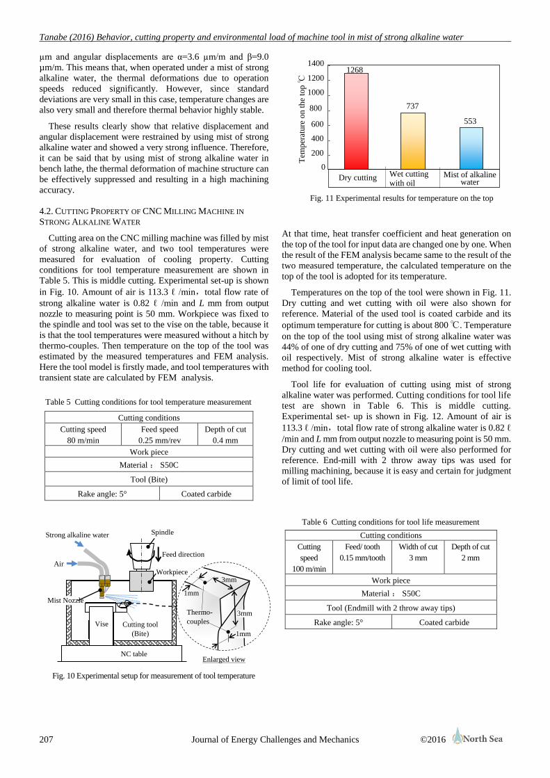
Tanabe (2016) Behavior, cutting property and environmental load of machine tool in mist of strong alkaline water
207 Journal of Energy Challenges and Mechanics ©2016
µm and angular displacements are α=3.6 µm/m and β=9.0
µm/m. This means that, when operated under a mist of strong
alkaline water, the thermal deformations due to operation
speeds reduced significantly. However, since standard
deviations are very small in this case, temperature changes are
also very small and therefore thermal behavior highly stable.
These results clearly show that relative displacement and
angular displacement were restrained by using mist of strong
alkaline water and showed a very strong influence. Therefore,
it can be said that by using mist of strong alkaline water in
bench lathe, the thermal deformation of machine structure can
be effectively suppressed and resulting in a high machining
accuracy.
4.2. CUTTING PROPERTY OF CNC MILLING MACHINE IN
STRONG ALKALINE WATER
Cutting area on the CNC milling machine was filled by mist
of strong alkaline water, and two tool temperatures were
measured for evaluation of cooling property. Cutting
conditions for tool temperature measurement are shown in
Table 5. This is middle cutting. Experimental set-up is shown
in Fig. 10. Amount of air is 113.3 ℓ /min,total flow rate of
strong alkaline water is 0.82 ℓ /min and L mm from output
nozzle to measuring point is 50 mm. Workpiece was fixed to
the spindle and tool was set to the vise on the table, because it
is that the tool temperatures were measured without a hitch by
thermo-couples. Then temperature on the top of the tool was
estimated by the measured temperatures and FEM analysis.
Here the tool model is firstly made, and tool temperatures with
transient state are calculated by FEM analysis.
At that time, heat transfer coefficient and heat generation on
the top of the tool for input data are changed one by one. When
the result of the FEM analysis became same to the result of the
two measured temperature, the calculated temperature on the
top of the tool is adopted for its temperature.
Temperatures on the top of the tool were shown in Fig. 11.
Dry cutting and wet cutting with oil were also shown for
reference. Material of the used tool is coated carbide and its
optimum temperature for cutting is about 800 ℃. Temperature
on the top of the tool using mist of strong alkaline water was
44% of one of dry cutting and 75% of one of wet cutting with
oil respectively. Mist of strong alkaline water is effective
method for cooling tool.
Tool life for evaluation of cutting using mist of strong
alkaline water was performed. Cutting conditions for tool life
test are shown in Table 6. This is middle cutting.
Experimental set- up is shown in Fig. 12. Amount of air is
113.3 ℓ /min,total flow rate of strong alkaline water is 0.82 ℓ
/min and L mm from output nozzle to measuring point is 50 mm.
Dry cutting and wet cutting with oil were also performed for
reference. End-mill with 2 throw away tips was used for
milling machining, because it is easy and certain for judgment
of limit of tool life.
Table 5 Cutting conditions for tool temperature measurement
Cutting conditions
Cutting speed
80 m/min
Feed speed
0.25 mm/rev
Depth of cut
0.4 mm
Work piece
Material : S50C
Tool (Bite)
Rake angle: 5° Coated carbide
Table 6 Cutting conditions for tool life measurement
Cutting conditions
Cutting
speed
100 m/min
Feed/ tooth
0.15 mm/tooth
Width of cut
3 mm
Depth of cut
2 mm
Work piece
Material : S50C
Tool (Endmill with 2 throw away tips)
Rake angle: 5° Coated carbide
Fig. 10 Experimental setup for measurement of tool temperature
Cutting tool
(Bite)
Enlarged view
Spindle
Feed direction
Workpiece
Strong alkaline water
g alkaline water
Air
Vise Vise
NC table
Mist Nozzle
3mm
Thermo-
couples
1mm
3mm
1mm
Fig. 11 Experimental results for temperature on the top
Tem
per
ature
on t
he
top ℃
Dry cutting Wet cutting with oil
Rake face
Flank face
1268
737
553
Mist of alkaline water
0
200
400
600
800
1000
1200
1400
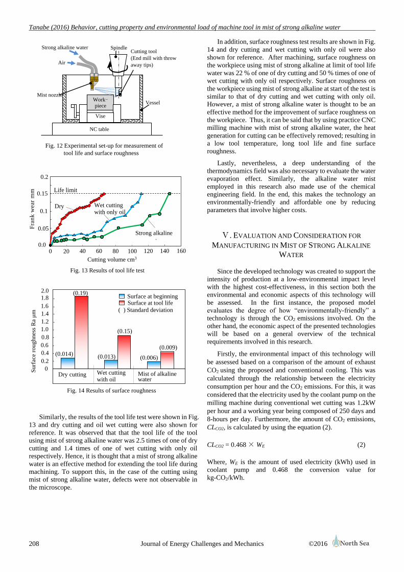
Tanabe (2016) Behavior, cutting property and environmental load of machine tool in mist of strong alkaline water
208 Journal of Energy Challenges and Mechanics ©2016
Similarly, the results of the tool life test were shown in Fig.
13 and dry cutting and oil wet cutting were also shown for
reference. It was observed that that the tool life of the tool
using mist of strong alkaline water was 2.5 times of one of dry
cutting and 1.4 times of one of wet cutting with only oil
respectively. Hence, it is thought that a mist of strong alkaline
water is an effective method for extending the tool life during
machining. To support this, in the case of the cutting using
mist of strong alkaline water, defects were not observable in
the microscope.
In addition, surface roughness test results are shown in Fig.
14 and dry cutting and wet cutting with only oil were also
shown for reference. After machining, surface roughness on
the workpiece using mist of strong alkaline at limit of tool life
water was 22 % of one of dry cutting and 50 % times of one of
wet cutting with only oil respectively. Surface roughness on
the workpiece using mist of strong alkaline at start of the test is
similar to that of dry cutting and wet cutting with only oil.
However, a mist of strong alkaline water is thought to be an
effective method for the improvement of surface roughness on
the workpiece. Thus, it can be said that by using practice CNC
milling machine with mist of strong alkaline water, the heat
generation for cutting can be effectively removed; resulting in
a low tool temperature, long tool life and fine surface
roughness.
Lastly, nevertheless, a deep understanding of the
thermodynamics field was also necessary to evaluate the water
evaporation effect. Similarly, the alkaline water mist
employed in this research also made use of the chemical
engineering field. In the end, this makes the technology an
environmentally-friendly and affordable one by reducing
parameters that involve higher costs.
Ⅴ. EVALUATION AND CONSIDERATION FOR
MANUFACTURING IN MIST OF STRONG ALKALINE
WATER
Since the developed technology was created to support the
intensity of production at a low-environmental impact level
with the highest cost-effectiveness, in this section both the
environmental and economic aspects of this technology will
be assessed. In the first instance, the proposed model
evaluates the degree of how “environmentally-friendly” a
technology is through the CO2 emissions involved. On the
other hand, the economic aspect of the presented technologies
will be based on a general overview of the technical
requirements involved in this research.
Firstly, the environmental impact of this technology will
be assessed based on a comparison of the amount of exhaust
CO2 using the proposed and conventional cooling. This was
calculated through the relationship between the electricity
consumption per hour and the CO2 emissions. For this, it was
considered that the electricity used by the coolant pump on the
milling machine during conventional wet cutting was 1.2kW
per hour and a working year being composed of 250 days and
8-hours per day. Furthermore, the amount of CO2 emissions,
CLCO2, is calculated by using the equation (2).
CLCO2 = 0.468 × WE (2)
Where, WE is the amount of used electricity (kWh) used in
coolant pump and 0.468 the conversion value for
kg-CO2/kWh.
Vessel
Fig. 12 Experimental set-up for measurement of
tool life and surface roughness
Cutting tool
(End mill with throw
away tips)
Spindle
Vise
Work-piece
NC table
Air
Strong alkaline water
Mist nozzle
Wet cutting with only oil
Fig. 13 Results of tool life test
Fra
nk
wear
mm
0.15
0.0
0.05
0.1
0.2
Dry
Strong alkaline
water mist
Life limit
Cutting volume cm3
80 120 0 40 20 60 100 140 160
Surf
ace
roughnes
s R
a μ
m
Wet cutting with oil
0
0.2
0.4
0.6
1.0
1.6
Dry cutting
(0.15)
( ) Standard deviation
(0.009)
Mist of alkaline water
(0.014) (0.006)
Surface at beginning Surface at tool life
0.8
1.2
1.4
1.8
2.0 (0.19)
(0.013)
Fig. 14 Results of surface roughness
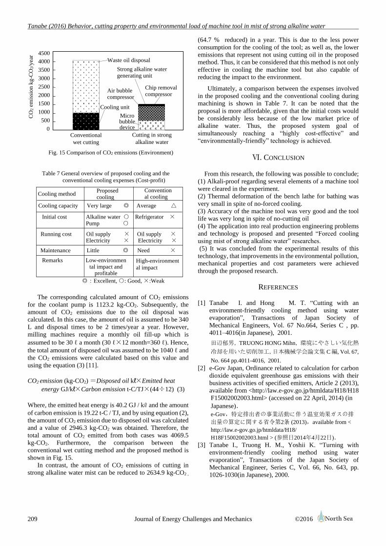
Tanabe (2016) Behavior, cutting property and environmental load of machine tool in mist of strong alkaline water
209 Journal of Energy Challenges and Mechanics ©2016
The corresponding calculated amount of CO2 emissions
for the coolant pump is 1123.2 kg-CO2. Subsequently, the
amount of CO2 emissions due to the oil disposal was
calculated. In this case, the amount of oil is assumed to be 340
L and disposal times to be 2 times/year a year. However,
milling machines require a monthly oil fill-up which is
assumed to be 30 ℓ a month (30 ℓ×12 month=360 ℓ). Hence,
the total amount of disposed oil was assumed to be 1040 ℓ and
the CO2 emissions were calculated based on this value and
using the equation (3) [11].
CO2 emission (kg-CO2) =Disposed oil kℓ×Emitted heat
energy GJ/kℓ×Carbon emission t-C/TJ×(44÷12) (3)
Where, the emitted heat energy is 40.2 GJ / kℓ and the amount
of carbon emission is 19.22 t-C / TJ, and by using equation (2),
the amount of CO2 emission due to disposed oil was calculated
and a value of 2946.3 kg-CO2 was obtained. Therefore, the
total amount of CO2 emitted from both cases was 4069.5
kg-CO2. Furthermore, the comparison between the
conventional wet cutting method and the proposed method is
shown in Fig. 15. In contrast, the amount of CO2 emissions of cutting in
strong alkaline water mist can be reduced to 2634.9 kg-CO2 ,
(64.7 % reduced) in a year. This is due to the less power
consumption for the cooling of the tool; as well as, the lower
emissions that represent not using cutting oil in the proposed
method. Thus, it can be considered that this method is not only
effective in cooling the machine tool but also capable of
reducing the impact to the environment.
Ultimately, a comparison between the expenses involved
in the proposed cooling and the conventional cooling during
machining is shown in Table 7. It can be noted that the
proposal is more affordable, given that the initial costs would
be considerably less because of the low market price of
alkaline water. Thus, the proposed system goal of
simultaneously reaching a “highly cost-effective” and
“environmentally-friendly” technology is achieved.
Ⅵ. CONCLUSION
From this research, the following was possible to conclude;
(1) Alkali-proof regarding several elements of a machine tool
were cleared in the experiment.
(2) Thermal deformation of the bench lathe for bathing was
very small in spite of no-forced cooling.
(3) Accuracy of the machine tool was very good and the tool
life was very long in spite of no-cutting oil
(4) The application into real production engineering problems
and technology is proposed and presented “Forced cooling
using mist of strong alkaline water” researches.
(5) It was concluded from the experimental results of this
technology, that improvements in the environmental pollution,
mechanical properties and cost parameters were achieved
through the proposed research.
REFERENCES
[1] Tanabe I. and Hong M. T. “Cutting with an
environment-friendly cooling method using water
evaporation”, Transactions of Japan Society of
Mechanical Engineers, Vol. 67 No.664, Series C , pp.
4011–4016(in Japanese), 2001.
田辺郁男,TRUONG HONG Mihn,環境にやさしい気化熱
冷却を用いた切削加工,日本機械学会論文集 C編, Vol. 67,
No. 664 pp.4011-4016, 2001.
[2] e-Gov Japan, Ordinance related to calculation for carbon
dioxide equivalent greenhouse gas emissions with their
business activities of specified emitters, Article 2 (2013),
available from <http://law.e-gov.go.jp/htmldata/H18/H18
F15002002003.html> (accessed on 22 April, 2014) (in
Japanese).
e-Gov,特定排出者の事業活動に伴う温室効果ガスの排
出量の算定に関する省令第2条 (2013),available from <
http://law.e-gov.go.jp/htmldata/H18/
H18F15002002003.html > (参照日2014年4月22日).
[3] Tanabe I., Truong H. M., Yoshii K. “Turning with
environment-friendly cooling method using water
evaporation”, Transactions of the Japan Society of
Mechanical Engineer, Series C, Vol. 66, No. 643, pp.
1026-1030(in Japanese), 2000.
Strong alkaline water generating unit
Fig. 15 Comparison of CO2 emissions (Environment)
CO
2 e
mis
sion k
g-C
O2/y
ear
Conventional
wet cutting
Cutting in strong
alkaline water
Chip removal compressor
Micro bubble device
Air bubble compressor
4000
4500
3500
3000
2500
2000
1500
1000
500
0
Waste oil disposal
Cooling unit
◎:Excellent, ○: Good, ×:Weak
Table 7 General overview of proposed cooling and the
conventional cooling expenses (Cost-profit)
Proposed cooling
Conventional cooling
Cooling method
Cooling capacity Very large ◎ Average △
Initial cost Alkaline water ○ Refrigerator × Pump ○
Running cost Oil supply × Oil supply × Electricity × Electricity ×
Maintenance Little ◎ Need ×
Remarks High-environment
al impact
Low-environmental impact and
profitable

Tanabe (2016) Behavior, cutting property and environmental load of machine tool in mist of strong alkaline water
210 Journal of Energy Challenges and Mechanics ©2016
田辺郁男,TRUONG HONG Mihn,吉井一夫,環境にや
さしい気化熱冷却を用いた切削加工(第1報,気化熱冷却
の効果と旋盤チップ冷却への適用),日本機械学会論文集
C編, Vol. 66, No. 643, pp.1026-1030, 2000.
[4] Tanabe, I., Ikeda, S. and Urano, K., Estimation of
optimum temperature for cooling oil on a spindle using
inverse analysis of neural network (Effect of relearning),
Transactions of Japan Society of Mechanical Engineers,
Series C, Vol. 69, No.679, pp. 819-824 (in Japanese),
2003.
田辺郁男,池田祥生,浦野好市,ニューラルネットワーク
の逆解法による主軸冷却油最適温度の推定(再学習の効
果),日本機械学会論文集 C編, Vol. 69, No. 679, pp.819-824,
2003.
[5] Tanabe I., Yamanaka K., Mizutani J. and Yamada Y. “A
new design of lathe structure for reducing thermal
deformation (Design of zero-center on three directions,
self-compulsory cooling and design of thermal
synchronism)”, Transactions of Japan Society of
Mechanical Engineers (Series C), Vol. 65, No.639, pp.
4508-4513 (in Japanese),1999.
田辺郁男,山中邦彦,水谷淳之介,山田泰宏,熱変形抑制
のための新しい旋盤構造設計(三次元零芯設計,セルフ強
制冷却,熱同期設計),日本機械学会論文集 C編, Vol. 65,
No. 639, pp.4508-4513, 1999.
[6] Tanabe I., Ye H. S., Iyama T. and Abe Y. “Control of tool
temperature using neural network for machining
work-piece with low thermal conductivity”, Transactions
of Japan Society of Mechanical Engineers (Series C), Vol.
77, No.776, pp. 1556-1564 (in Japanese), 2011.
田辺郁男,イエー・トット・ソー,井山徹郎,阿部洋太朗,
低熱伝導材料加工のためのニューラルネットワークを用
いた工具温度管理,日本機械学会論文集 C編, Vol. 77, No.
776, pp.1556-1564, 2011.
[7] Shiddaira S., Material science for corrosion and corrosion
resistance (in Japanese), AGNE technological center,
pp.30-32, 255-257, 287-288, 1995.
下平三郎, 腐食・防食の材料科学, アグネ技術センター,
pp.30-32, 255-257, 287-288, 1995.
[8] Shintani S., Hand book for cutting fluid, Kogyo Chosakai
Publishing Co., Ltd., (2004), pp. 33-48 (in Japanese). 新谷滋記,切削油剤ハンドブック,株式会社 工業調
査会, pp. 33-48, 2004.
[9] Okada M., Hosokawa A., Asakawa N., Fujita Y. and Ueda
T. “Influence of minimum quantity lubrication on tool
temperature in end milling of difficult-to-cut materials
having low thermal conductivity”, Transactions of Japan
Society of Mechanical Engineers (Series C), Vol. 78,
No.792, pp. 3093-3103 (in Japanese), 2012. 岡田将人, 細川晃, 浅川直紀, 藤田祐介, 上田隆司,低熱
伝導率難削材のエンドミル加工におけるMQLの工具温度
への影響,日本機械学会論文集C編, Vol. 78, No. 792( 2012),
pp.3093-3103.
[10] Tanabe I. “Development of forced cooling using mist of
strong alkaline water for restraining thermal deformation
on a machine tool”, MM-science journal, DECEMBER ,
pp. 521-526, 2014.
[11] Enviroment agency, “Law (enforce No3) for Global
Warming Countermeasures in Japan-(Exhaust coefficient
list)” , 2006.

ISSN 2056-9386
Volume 3 (2016) issue 4, article 6
211 ©2016
Korea’s policies, R&D investment and competitiveness
in the LED industry
韩国在光敏二极管行业的政策,研发投资和竞争力
Joon Han(韓準)1, Chul-Ho Park(朴哲皞)1*, Ji-Sun Ku(具智善)1, Ho-Sik Chon(全浩植)2
1 Center for Climate Technology Cooperation, Green Technology Center Korea, Seoul, Korea 2 Division of Policy Research, Green Technology Center Korea, Seoul, Korea
[email protected] (Joon Han); [email protected] (Chul-Ho Park)
Accepted for publication on 8th January 2017
Abstract - The Korean government released its plan to carry
out intensive short-term investment in LED-related R&D
projects to develop LED as a growth engine for Korea in the near
future. It also announced ambitious goals regarding how to
support LED technology and distribute it. In addition, it
designated LED as a suitable business for small- and
medium-sized enterprises (SMEs) to encourage the development
of SMEs in the field. However, Korea’s LED industry faces
difficulties because of strong challenges from globalized
multinational companies and the lack of fundamental technology.
This research is to review Korea’s LED policies and plans, its
R&D investment in the field for years, and its competitiveness so
as to assess the correlations of the three. The amount of R&D
investment in the field can be a clear example of the
government’s support to nurture the industry and its
competitiveness in the LED industry can be a good index to
determine whether such investment is successful or not. Lastly,
the research provides some suggestions for the vitalization of the
LED industry in Korea.
Keywords - LED, Policy, R&D investment, Competitiveness,
Korea
I. INTRODUCTION
LED (Light-emitting diode) lighting is a lighting fixture
consisting of a LED light source and module. It has
advantages such as long-life and highly efficient lighting,
which contribute to reducing energy consumption and CO2
emissions. Because of these advantages, the Korean
government designated it as one of 27 Core Green
Technologies 1 (NST, 2009). And the Korean government
1 27 core green technologies are as followings. (1) Monitoring
and modeling for climate change (2) Climate change
assessment and adaptation (3) Silicon-based solar cells (4)
planned to promote the domestic LED industry as an
export-led green industry through intensive short-term
investment which can lead to improved price competitiveness
and localized technology (PCGG, 2009).
However, the Korean LED industry experiences a lot of
difficulties as, basically, it lacks fundamental technology and
is aggressively challenged by foreign businesses equipped
with vertical integration, high quality and low cost. Moreover,
there was a serious conflict between SMEs and large
businesses over the issue of designating the industry as an
SME-suitable industry, which, some evaluated, might further
lower Korea’s LED competitiveness. In this regard, it is
required to evaluate the current situations from diverse
perspectives as they happened despite the government’s
policies to nuture the industry.
This research is to review the Korean government’s policies
and plans to develop, and distribute LED technology. It deals
with the government’s R&D investment in the field for years
Non-silicon based solar cells (5) Bio energy (6) Light water
reactors (7) Next-generation fast reactors (8) Nuclear fusion
energy (9) Hydrogen energy (10) Fuel cell (11) Plant growth
promotion (12) Integrated gasification combined cycle (13)
Green cars (14) Infrastructure for intelligent transport and
logistics (15) Green city and urban renaissance (16) Green
buildings (17) Green Process technology (18) LED/green IT
(19) IT-combined electric machines (20) Secondary batteries
(21) CO₂ capture, storage, and sequestration (22) Non-CO₂
sequestration (23) Assessment and management of water
quality (24) Alternative water resources (25) Waste reduction,
recycling and energization (26) Monitoring and processing of
hazardous substances (27) Virtual reality
Han et al. (2017) Korea’s policies, R&D investment and competitiveness in the LED industry
212 Journal of Energy Challenges and Mechanics ©2016
and its competitiveness so as to assess the correlations of the
policies, R&D investment and competitiveness. The amount
of R&D investment of the government in the LED industry
can be a clear example that shows the level of the
government’s nurturing policies. Its competitiveness in the
LED industry, which is the result of such investment, can be
an important index to determine whether the investment is
successful or not. Through this, the research also provides
some suggestions for the vitalization of the LED industry in
Korea.
II. METHODS
For this study, three different aspects were examined:
national LED promotion policies and plans, government
expenditure on LED R&D, and the level of LED technology.
First, the national master plan released by the government and
its reports on LED were reviewed.2 It also goes over the issue
of designating the LED industry as an SME-suitable industry
because the SME-suitable industry designation scheme has a
lot of impact on Korea’s LED industry. Second, the
government’s expenditure on LED R&D in Korea was
analyzed. The national R&D database named ‘National
Science & Technology Information Service (NTIS)’ was used.
It is a portal service offered by the National Science &
Technology Council and provides information on national
R&D projects including R&D-related businesses, projects,
human resources, lab equipment & devices, research
outcomes, etc.3 Third, the competitiveness of Korea’s LED
technology was assessed compared with those of major
developed countries. Finally, based on the analysis, this study
suggests some points for policies to promote the LED
industry.
III. NATIONAL POLICY AND PLANS FOR THE LED
INDUSTRY IN KOREA
3.1. NATIONAL STRATEGY TO PROMOTE THE LED INDUSTRY
The previous Korean government (Feb. 2008 ~ Feb. 2013)
announced “Green Growth” as a national agenda and
emphasized green technology which could facilitate not only
economic development but also environmental conservation.
It designated LED technology as green technology that should
be quickly developed, demonstrated, distributed and timely
commercialized through intensive short-term investment. By
localizing LED components and enhancing their price
competitiveness, the LED industry was expected to be
2 The statistics related to the distribution of LED in Korea
hasn’t been properly accumulated by the government yet so
this research doesn’t deal with the evaluation on it. 3 NTIS homepage (http://www.ntis.go.kr)
developed as a leading export industry of Korea (PCGG,
2009).
The Korean government set the goals for the world market
share of Korean LED products at 20% and their luminous
efficiency (210 lm/W) by 2020 (joint assessment by related
departments, 2012). The LED Lighting 2060 Plan was
announced where the national goals for the LED distribution
rate would be 100% in public offices and 60% in the whole
country by 2020. It was also planned to improve LED
efficiency and decrease its price through increased R&D
investment, to enhance consumer awareness about domestic
LED lighting through follow-up services, and to establish a
collaboration system between large companies and SMEs
(MKE, 2011). Under the National Energy Master Plan 2.0, all
lamps installed in subway, tunnels, public offices and
passenger terminals should be replaced with LED ones by
2020.
3.2. DESIGNATION OF LED AS AN SME-SUITABLE INDUSTRY
Designating LED as an SME-suitable industry was an
important issue in the Korean LED market in that it
substantially affects Korea’s competitiveness in the industry.
The Korean government introduced the SME-suitable industry
designation scheme in 2011. It is aimed to foster the
competitiveness and growth of Korea’s SMEs by restricting
the entry and expansion of large companies into the field. And
LED production was included in the scheme in November
2011. After the decision, large companies’ sales and
production of LED and its components in the consumer market
were prohibited in Korea except for multi-faceted reflector
(MR), parabolic anodized reflector (PAR), and bulb type LED.
It was expected to ease economic polarization between large
companies and SMEs in the LED industry. However, there
was a serious conflict between them over the policy. While
SMEs supported the scheme, large domestic companies
opposed it. Large companies insisted that domestic SMEs
would play just a simple role of assembling parts in LED
production while foreign companies would make inroads into
the domestic market. Looking at the result after the
designation, they insisted it was doubtful whether the scheme
really contributed to improving domestic competitiveness and
supporting the economic growth of SMEs in the domestic
market. Actually, the competition among domestic SMEs in
the LED market has become intensified and has made
domestic SMEs concentrate on producing low price LED
products. This caused an invasion of foreign LED companies
with low-priced, high-quality LED products and the
deterioration of the technological competitiveness of SMEs. It
was reported that foreign LED companies occupied up to
60~70% of the consumer LED market in Korea (KCCP,
2013).
In January 2015, the Korean government finally cancelled
the designation of LED as a suitable market for SMEs. In line
with it, large domestic companies and SMEs made a
‘cooperation agreement for the development of LED lighting

Han et al. (2017) Korea’s policies, R&D investment and competitiveness in the LED industry
213 Journal of Energy Challenges and Mechanics ©2016
products’ without government enforcement to strengthen
global competitiveness of the Korean LED industry and
promote mutual cooperation. (KCCP, 2015). According to the
agreement, large domestic companies would not enter the
domestic LED procurement market until 2018, making an
effort to promote the domestic LED industry through signing
an Original Equipment Manufacturing (OEM) and/or an
Original Design Manufacturing (ODM) with SMEs.
This agreement could be reached because of the
understanding that it is necessary for the two players to
cooperate for the vitalization of Korea’s LED industry and
mutual growth and prosperity. In fact, the global LED lighting
market is dominated by three major lightning companies -
namely Osram, Philips and GE - which strengthen their
competitiveness through vertical integration (Sanderson et al,
2008). Against this backdrop, it is essential to establish such
collaboration system in Korea. In fact, there used to be some
attempts led by large companies to achieve vertical integration
in the Korean LED industry; however, such plans were given
up in the middle or substantially changed soon. It was because
the vertical integration by large domestic businesses didn’t
create much comparative advantage while foreign businesses
entering the Korean market could expand their production
capacity and lower production costs through it. In this regard,
it is necessary to strengthen collaboration between SMEs and
large companies so that such close cooperation can produce
advantages like the ones vertical integration can create.
IV. GOVERNMENT EXPENDITURE ON LED R&D IN
KOREA
4.1. ANNUAL GOVERNMENT EXPENDITURE ON LED R&D IN
KOREA
Annual government expenditure on LED R&D4 in Korea
and its relative proportion to total government R&D
expenditure on green technology between 2011 and 2014 are
presented in Fig. 1. The Korean government spent 20.1 million
USD in 2011, 20.4 million USD in 2012, 32.7 million USD in
2013 and 108.7 million USD in 2014, accounting for 0.9%,
0.8%, 1.2% and 4.3% of annual total government R&D
expenditure on green technology respectively. During the
period from 2011 to 2014, the rate of government expenditure
on LED R&D had increased by 5.4 times. It is quite a big
figure considering the fact that Korea’s total R&D investment
in green technology increased by 1.1 times during the period.
(MSIP>C, 2014). Such huge increase in the government’s
R&D investment in LED fit its policy to nurture the industry.
4 Ministry of Science, ICT and Future Planning (MSIP) and
Green Technology Center (GTC) provide a report including
annual government expenditure on green technology.
Source: MSIP & GTC (2015)
Fig.1, Annual government expenditure on LED R&D in Korea
between 2011 and 2014
4.2. ANNUAL GOVERNMENT EXPENDITURE ON DIFFERENT
STAGES OF LED R&D
Depending on R&D stages, the national R&D could be
classified into ‘basic research’, ‘applied research’ and
‘experimental development’ (OECD, 2002). Investment in
basic research is the investment to support theoretical or
experimental researches to be conducted to acquire new
knowledge of natural phenomena or observable facts without
any particular use or application. Private enterprises invest in
basic research to prepare technologies required for the next
generation. Applied research is the creative study to obtain the
new scientific knowledges for specific practical aim or
objective and typically utilizes results obtained from basic
researches. The business enterprise sector creates new project
to explore promising results of basic research program. The
results of applied research are typically valid for limited
number of products, methods, operations or systems.
Experimental development is systematic work to improve
those already produced or installed or to produce new
materials, products and devices through knowledge gained
from basic research, applied research and practical experience.
The annual government expenditure on different stages of
LED R&D in Korea between 2011 and 2014 is shown in Fig.
2. A large amount of LED R&D budget was used for the stage
of ‘experimental development’ research in Korea, ranging
from 44.3% ~ 63.1% of total government expenditure on LED
R&D annually. The share of experimental development
increased greatly at 63.1% in 2014. Such increase can be
interpreted as the result of the Korean government’s LED
promotion policies, one of which considered LED lighting as
the technology needed to be developed, demonstrated, and
distributed within a short period of time. (PCGG, 2009). In
order to obtain a tangible outcome, the Korean government

Han et al. (2017) Korea’s policies, R&D investment and competitiveness in the LED industry
214 Journal of Energy Challenges and Mechanics ©2016
intensively invested in LED R&D, especially in the stage of
‘experimental development’ research.
However, in order for LED technology to be a real growth
engine, Korea should have fundamental technology. It can be
possible by expanding investment in basic research among the
four LED R&D stages. As Korea’s LED R&D is concentrated
on experimental development and Korea’s LED companies
fail to obtain fundamental LED technology, the investment
hasn’t made noticeable results like the industry’s growing
rapidly and becoming a growth engine as the government
expected. In this regard, it is very important to increase LED
R&D budgets for ‘basic research not only for the development
of the LED industry, but also for the development of
next-generation LED products in Korea.
Source: MSIP & GTC (2015)
Fig.2, Annual government expenditure on different stages of LED
R&D in Korea between 2011 and 2014
4.3. ANNUAL GOVERNMENT EXPENDITURE ON LED R&D LED
BY DIFFERENT INSTITUTIONS AND COMPANIES
In Korea, most national projects for LED R&D are carried
out by Combined Research Institutions (CRIs), University and
Colleges (U&Cs), and SMEs. Others include Public Research
Institutions (PRIs), Large Enterprises (LEs) and High
Potential Enterprises (HPEs). As presented in Fig. 3, 37.1%
and 38.4% of annual total government expenditure on LED
R&D in 2011 and 2012 were allocated to U&Cs respectively,
contributing to its highest proportion of R&D activities in
Korea. Then from 2013, SMEs started to take the largest share
and it reached at 41.2% in 2014. This seems to be affected by
the decision of the Korean government to designate LED
production as a suitable business for SMEs.
Source: MSIP & GTC (2015)
Fig.3, Annual government expenditure on LED R&D carried out by
different institutions and companies between 2011 and 2014
V. COMPETITIVENESS OF KOREA’S LED
TECHNOLOGY
It is a global trend to make a high-efficient, low-priced LED
lighting. Competition among LED companies is more
intensified than ever before, especially in the field of lighting
modules and lighting engines. At present, Korean companies
have LED technologies with 190lm/W of luminous efficiency
and over 50,000 hours of lifetime and have made efforts to
improve energy efficiency and price competitiveness of LED
products.
This study evaluated the competitiveness of Korean LED
lighting products by comparing it with those of major
developed countries. Fig. 4 shows Korea’s technology
competitiveness, price competitiveness, and quality
competitiveness on different stages of the LED supply chain
against major competitors, namely, the US, Japan and
European countries (Germany, Italy, the Netherlands, etc.) As
shown in Fig. 4, Korean LED price levels are quite
competitive in comparison to those of major developed
countries. However, the competitiveness of Korean LED
product’s quality and technology is relatively inferior to those
of major developed countries. In addition, the localization
ratio of LED materials is only 40% in Korea, while those of
chips, modules, optical parts and heat sinks used for LED
production are 60 to 80% (KAPID, 2014). The reason why the
competitiveness of Korean LED materials is low is that
Korean companies do not have enough fundamental
technology. The Korean LED industry lacks fundamental
technology such as a LED packaging technology and has a
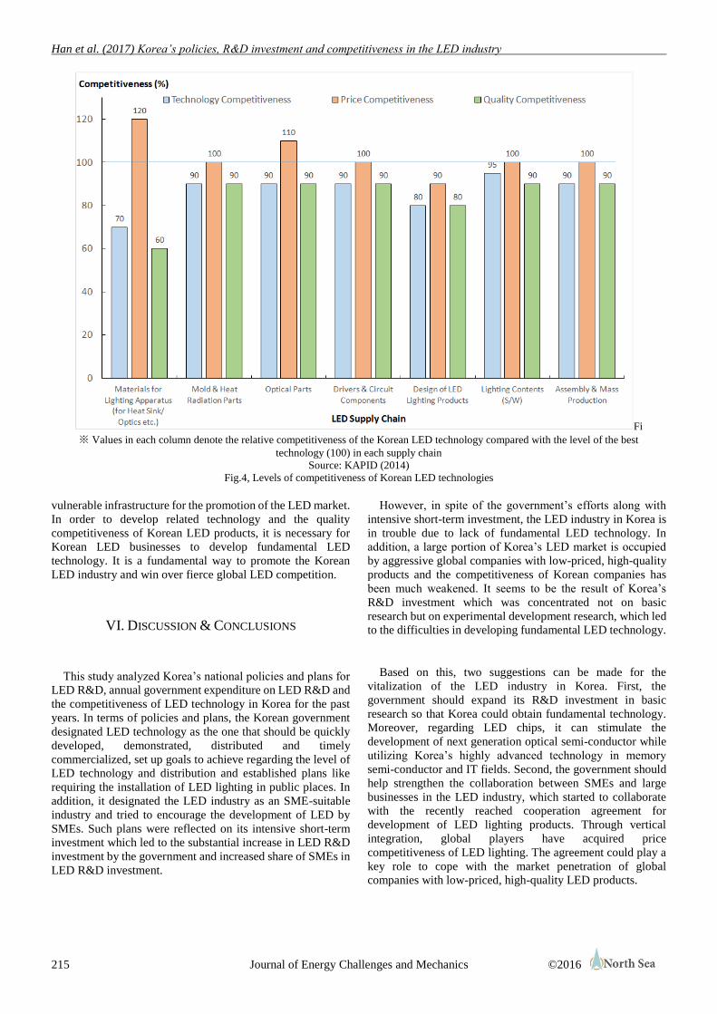
Han et al. (2017) Korea’s policies, R&D investment and competitiveness in the LED industry
215 Journal of Energy Challenges and Mechanics ©2016
vulnerable infrastructure for the promotion of the LED market.
In order to develop related technology and the quality
competitiveness of Korean LED products, it is necessary for
Korean LED businesses to develop fundamental LED
technology. It is a fundamental way to promote the Korean
LED industry and win over fierce global LED competition.
VI. DISCUSSION & CONCLUSIONS
This study analyzed Korea’s national policies and plans for
LED R&D, annual government expenditure on LED R&D and
the competitiveness of LED technology in Korea for the past
years. In terms of policies and plans, the Korean government
designated LED technology as the one that should be quickly
developed, demonstrated, distributed and timely
commercialized, set up goals to achieve regarding the level of
LED technology and distribution and established plans like
requiring the installation of LED lighting in public places. In
addition, it designated the LED industry as an SME-suitable
industry and tried to encourage the development of LED by
SMEs. Such plans were reflected on its intensive short-term
investment which led to the substantial increase in LED R&D
investment by the government and increased share of SMEs in
LED R&D investment.
However, in spite of the government’s efforts along with
intensive short-term investment, the LED industry in Korea is
in trouble due to lack of fundamental LED technology. In
addition, a large portion of Korea’s LED market is occupied
by aggressive global companies with low-priced, high-quality
products and the competitiveness of Korean companies has
been much weakened. It seems to be the result of Korea’s
R&D investment which was concentrated not on basic
research but on experimental development research, which led
to the difficulties in developing fundamental LED technology.
Based on this, two suggestions can be made for the
vitalization of the LED industry in Korea. First, the
government should expand its R&D investment in basic
research so that Korea could obtain fundamental technology.
Moreover, regarding LED chips, it can stimulate the
development of next generation optical semi-conductor while
utilizing Korea’s highly advanced technology in memory
semi-conductor and IT fields. Second, the government should
help strengthen the collaboration between SMEs and large
businesses in the LED industry, which started to collaborate
with the recently reached cooperation agreement for
development of LED lighting products. Through vertical
integration, global players have acquired price
competitiveness of LED lighting. The agreement could play a
key role to cope with the market penetration of global
companies with low-priced, high-quality LED products.
Fi
※ Values in each column denote the relative competitiveness of the Korean LED technology compared with the level of the best
technology (100) in each supply chain
Source: KAPID (2014)
Fig.4, Levels of competitiveness of Korean LED technologies

Han et al. (2017) Korea’s policies, R&D investment and competitiveness in the LED industry
216 Journal of Energy Challenges and Mechanics ©2016
REFERENCES
[1] Joint assessment by related departments in Korea.
Assessment on LED development and distribution
policies and follow-up measures. an agenda for the 6th
assessment meeting. 2012.
[2] Korea Association for Photonics Industry Development
(KAPID). Survey on the Utilization of lighting Apparatus
and Study on Saving Lighting Power Consumption.
Ministry of Trade, Industry and Energy (MOTIE), 2014.
[3] Korean Commission for Corporate Partnership (KCCP).
KCCP's position on the article of The Seoul Economic
Daily(11.17) related with businesses suitable for SMEs.
2013.
[4] Korean Commission for Corporate Partnership (KCCP).
Corporate partnership for cooperation and development
of LED lighting product between large companies and
SMEs. 2015.
[5] Ministry of Science, ICT and Future Planning (MSIP)
and Green Technology Center (GTC). Statistics
Yearbook 2014 of Green Technology - Research and
Development. 2015.
[6] Ministry of Knowledge Economy (MKE). Proposing
"2060 LED Lighting Plan" for Green Lighting Society.
2011.
[7] National Research Council of Science & Technology
(NST). Green Technology R&D Comprehensive Plan.
2009.
[8] OECD. Frascati Manual: Proposed standard practice
for surveys on research and experimental development.
2002. http://www.oecd.org/sti/frascatimanual
[9] Presidential Committee on Green Growth (PCGG). Core
Green Technologies and Commercialization Strategies.
Agenda for the 3th Meeting of Committee on Green
Growth. 2009.
[10] S. W. Sanderson, K. L. Simons, J. L. Walls, and Y. Lai.
“Lighting Industry: Structure and Technology in the
Transition to Solid State,” 2008 Industry Studies
Conference Paper, 2008.