Volume 20, Number 3, January 2018 - bi.go.id · volume 20, number 3, january 2018 issn 1410 - 8046...
153
Volume 20, Number 3, January 2018 ISSN 1410 - 8046 THE EFFECT OF FINANCIAL LIBERALIZATION AND CAPITAL FLOWS ON INCOME VOLATILITY IN ASIA-PACIFIC Feriansyah, Noer Azam Achsani, Tony Irawan ONLINE BANKING IMPLEMENTATION: RISK MAPPING USING ERM APPROACH Mochamad Aji Jaya Sakti, Ferry Syarifuddin, Noer Azam Achsani MARKET STRUCTURE AND COMPETITION OF SHARIAH BANKING IN INDONESIA Sunarmo ANNS-BASED EARLY WARNING SYSTEM FOR INDONESIAN ISLAMIC BANKS Saiful Anwar, A.M. Hasan Ali SELECTING EARLY WARNING INDICATIORS FOR IDENTIFYING CORPORATE SECTOR DISTRESS: STRENGTHENING CRISIS PREVENTION Arlyana Abubakar, Rieska Indah Astuti, Rini Oktapiani NOWCASTING HOUSEHOLD CONSUMPTION AND INVESTMENT IN INDONESIA Tarsidin, Idham, Robbi Nur Rakhman
Transcript of Volume 20, Number 3, January 2018 - bi.go.id · volume 20, number 3, january 2018 issn 1410 - 8046...

Volume 20, Number 3, January 2018
ISSN 1410 - 8046
THE EFFECT OF FINANCIAL LIBERALIZATION AND CAPITAL FLOWS ON INCOME VOLATILITY IN ASIA-PACIFIC
Feriansyah, Noer Azam Achsani, Tony Irawan
ONLINE BANKING IMPLEMENTATION:RISK MAPPING USING ERM APPROACH
Mochamad Aji Jaya Sakti, Ferry Syarifuddin, Noer Azam Achsani
MARKET STRUCTURE AND COMPETITION OFSHARIAH BANKING IN INDONESIA
Sunarmo
ANNS-BASED EARLY WARNING SYSTEMFOR INDONESIAN ISLAMIC BANKS
Saiful Anwar, A.M. Hasan Ali
SELECTING EARLY WARNING INDICATIORS FORIDENTIFYING CORPORATE SECTOR DISTRESS:
STRENGTHENING CRISIS PREVENTIONArlyana Abubakar, Rieska Indah Astuti, Rini Oktapiani
NOWCASTING HOUSEHOLD CONSUMPTION ANDINVESTMENT IN INDONESIA
Tarsidin, Idham, Robbi Nur Rakhman
Bulletin of Monetary Econom
ics and Banking - Volum
e 20, Num
ber 3, January 2018

Bulletin of Monetary Economics and BankingBank Indonesia
PatronBoard of Governors of Bank Indonesia
Editor-in-ChiefDr. Perry WarjiyoBank Indonesia, University of Indonesia, Indonesia
Board of EditorsProf. Dr. Anwar Nasution, University of Indonesia, IndonesiaProf. Dr. Miranda S. Goeltom, University of Indonesia, IndonesiaProf. Dr. Insukindro, Gadjah Mada University, IndonesiaProf. Dr. Iwan Jaya Azis, Cornell University, USAProf. Takahiro Akita, Rikkyo University, JapanProf. Dr. Iftekhar Hasan, Fordham University, USAProf. Dr. Masaaki Komatsu, Hiroshima Jogakuin University, JapanDr. M. Syamsuddin, Bandung Institute of Technology, IndonesiaDr. Perry Warjiyo, Bank Indonesia, University of Indonesia, IndonesiaDr. Iskandar Simorangkir, Bank Indonesia, University of Indonesia, IndonesiaDr. Solikin M. Juhro, Bank Indonesia, University of Indonesia, IndonesiaDr. Haris Munandar, Bank Indonesia, IndonesiaDr. M. Edhie Purnawan, Gadjah Mada University, IndonesiaDr. Burhanuddin Abdullah, Institut Manajemen Koperasi Indonesia, Indonesia
Managing EditorDr. Ferry Syarifuddin, Bank Indonesia, Bogor Agriculture University, IndonesiaDr. Andi M. Alfian Parewangi, University of Indonesia, Indonesia
The Bulletin of Monetary Economics and Banking is a refereed international journal publishes original manuscripts on subject areas including monetary economics, finance, banking, macroprudential, payment systems, international economics and development economics.
This bulletin is published by Bank Indonesia Institute, Bank Indonesia. Contents and research outcome in the articles of this bulletin are entirely the responsibility of the authors and do not represent Bank Indonesia’s views.
The bulletin is published quarterly in January, April, July, and October. We invite all authors to write in this bulletin. Manuscript is delivered in soft files to Bank Indonesia Institute, Bank Indonesia, Sjafruddin Prawiranegara Tower, 21st Floor, Jl. M.H. Thamrin No. 2, Jakarta, website BMEB: (www.journalbankindonesia.org) and email : [email protected].
Accredited - SK: 36A / E / KPT / 2016

Bulletin of Monetary Economics and Banking
Volume 20, Number 3, January 2018
CONTENT
The Effect of Financial Liberalization and Capital Flows on Income Volatilityin Asia-PacificFeriansyah, Noer Azam Achsani, Tony Irawan _________________________ 257
Online Banking Implementation: Risk Mapping Using ERM ApproachMochamad Aji Jaya Sakti, Ferry Syarifuddin, Noer Azam Achsani ________ 279
Market Structure and Competition of Shariah Banking in IndonesiaSunarmo _________________________________________________________ 307
Anns-Based Early Warning System for Indonesian Islamic BanksSaiful Anwar, A.M. Hasan Ali _______________________________________ 325
Selecting Early Warning Indicatiors forIdentifying Corporate Sector Distress: Strengthening Crisis PreventionArlyana Abubakar, Rieska Indah Astuti, Rini Oktapiani _________________ 343
Nowcasting Household Consumption and Investment in IndonesiaTarsidin, Idham, Robbi Nur Rakhman ________________________________ 375

THE EFFECT OF FINANCIAL LIBERALIZATION ANDCAPITAL FLOWS ON INCOME VOLATILITY IN ASIA-PACIFIC
Feriansyah1 2, Noer Azam Achsani2, Tony Irawan3
1. Jalan mujahidin lorong langgar shotto no. 635, 26 ilir, Kota Palembang, Sumatera Selatan, 30135. HP: +6289639167250. E-mail: [email protected]. Departement of Economics, Bogor Agricultural University, Indonesia. E-mail: [email protected]. Departement of Economics and School of Management and Business, Bogor Agricultural University, Indonesia. E-mail: [email protected]. Departement of Economics, Bogor Agricultural University, Indonesia. E-mail: [email protected]
This paper examines the effect of financial liberalization on income volatility focused on the direction of capital flows in the Asia-Pacific region. By using a dynamic panel model, this study investigates the effect of financial liberalization on income volatility in 19 Asia-Pacific countries over the period 1976-2015. The results show that the financial liberalization in the Asia-Pacific region associated with low income volatility is only perceived by developed countries, while not for developing countries. This paper also investigates the effect of capital flows on different types of directions. The results show that capital outflows will be associated with low income volatility, whereas capital inflows will be associated with high income volatility. The negative effect of financial liberalization on income volatility in developing countries is caused by the majority of those countries holding larger capital inflows, compared to capital outflows. Therefore, the excess capital inflows in developing countries increase the pressure and the vulnerability to the crisis.
Keywords: Asia-Pacific, Capital Flows, Financial Liberalization, Macroeconomic VolatilityJEL Classification: F41, F36
ABSTRACT

Bulletin of Monetary Economics and Banking, Volume 20, Number 3, January 2018258
I. INTRODUCTIONSince 1990, the economic globalization has created a world trade liberalization followed by integrated global financial markets (Rajan, 2001). Financial market transactions freedom is characterized by an increasingly free movement of capital in industrialized countries, especially countries in Europe and America. The increasing degree of financial sector liberalization in the industrialized countries subsequently has spread to various regions in the world, especially countries in the Asia-Pacific. Chinn and Ito (2008) revealed that since 1970, the financial openness of developing countries in the Asia-Pacific region has the greatest level relative to other regions. The high financial market activity in Asia-Pacific according to Borensztein and Loungani (2011) has shown that the integrated capital flows in the Asia-Pacific region and the mobility of capital has moved freely, thus making most of the liabilities of companies and banking countries in Asia-Pacific region began to be dominated by various foreign currency units.
Figure 1 shows de jure and de facto financial liberalization data movements in the Asia-Pacific. De jure level of financial liberalization shows the index of financial liberalization issued by Chinn and Ito (2008). This variable calculates the degree of capital account openness to foreign funding in a country. Meanwhile, the financial openness representing de facto financial liberalization is calculated using the measurement of financial openness of Lane and Milesi-Ferretti (2007). The method of calculating financial openness is by summing the total capital inflows and outflows divided by gross domestic product. The degree of financial openness in the Asia-Pacific has always increased over time. The data show that in 1976 the average degree of financial openness in the Asia-Pacific was only 0.45 index unit, then increased eightfold by the year 2015 to 3.4 index units. Similarly, the degree of
Figure 1.Average Degree of Financial Liberalization and Openness in Asia-Pacific Countries
0
0,5
1
1,5
2
2,5
3
3,5
4
1976
1980
1984
1988
1992
1996
2000
2004
2008
2012
Index Financial Openness (de facto)
Asia-Pacific

The Effect of Financial Liberalization and Capital Flows on Income Volatility in Asia-Pacific 259
financial liberalization shows an increasing trend over time, except in 1997 which decreased due to the global financial crisis.
Economic globalization that makes the financial sector more integrated in the Asia-Pacific region becomes an interesting phenomenon to be observed. One of the reasons is, financial liberalization can affect the level of economic stability. According to Mirdala et al. (2015), the development of studies and empirical research on financial liberalization in the world began because of the effects of financial liberalization on the economy. These findings concluded that the liberalization process of capital flows led by industrialized countries which have been a stimulus in improving the efficiency of wealth allocation and sharing international financial risks. The allocation efficiency of wealth and the sharing of international risks will then affect the growth and maintain the economic stability. In addition to the benefit from allocation efficiency and risk sharing internationally, the flow of capital across countries will also determine economic outcomes and will further influence the volatility of macroeconomic variables. Ultimately, the risk of such macroeconomic volatility will affect the economic growth and will implicate the level of welfare in an economy indirectly.
Kose, Prasad, and Terrones (2006) have proved that the economic globalization marked by an increasing in the volume of international trade and financial flows has weakened the negative relationship between volatility and economic growth. Similarly, Ahmed and Suardi (2009), Pancaro (2010), Torki (2012) and Mirdala et al. (2015) have found that financial openness has contributed significantly to influencing income and consumption volatility. The integrated economy will contribute by lowering the volatility of output and consumption. The findings are reinforced by Ozcan, Sorensen, and Yosha (2013) who revealed that the integrated flow of cross-border capital will maintain fluctuations in macroeconomic variables.
Therefore the positive benefits of financial liberalization are still debated both in theory and empirical studies. Kose, Prasad, and Terrones (2003) revealed that the relationship between financial liberalization to income and consumption volatility
Asia-Pacific
0,4
0,45
0,5
0,55
0,6
0,65
0,7
0,75
1976
1980
1984
1988
1992
1996
2000
2004
2008
2012Index Financial Liberalization (de jure)

Bulletin of Monetary Economics and Banking, Volume 20, Number 3, January 2018260
is still not conclusive and well explained. The lack of clarity on the relationship is due to the two forces in financial openness. These forces may increase or reduce the economic volatility. International financial openness can reduce volatility due to diversification in risk sharing. On the other hand, financial openness can lead to greater specialization and increase volatility levels. According to Mirdala et al. (2015), the advantages of financial liberalization in reducing economic instability are affected by economic conditions within a country. The existence of financial market openness empirically gives more positive effect for developed countries while not for developing countries.
The influence of financial liberalization on the uncertainty of the economic remains unclear. Therefore, an analysis of the impact of financial liberalization on income volatility in the Asia-Pacific region becomes important to be investigated. Since the Asia-Pacific region is still dominated by developing countries, this study will ultimately provide an important conclusion whether the presence of financial liberalization in the Asia-Pacific region will provide benefits or not. Moreover, the influence of the direction of capital flow becomes an important consideration in this study. The behavior of capital inflows and capital outflows in influencing income volatility is expected to explain the possible effect of different financial liberalization on income volatility, especially in developed and developing countries.
II. THEORY Ramey and Ramey (1995) have proved that the volatility and growth output are negatively correlated. This indicates that countries with high volatility have low economic growth. The relationship concludes that the volatility of output that affects economic growth indirectly plays an important role because it will have implications for the level of welfare in an economy. The existence of these empirical relationships makes Kose et al. (2006) to examine the relationships between outputs volatility and growth in the context of globalization in light of the phenomenon of trade openness and financial integration in many countries by interacting the financial integration and trade openness to output volatility. The results showed that financial integration and trade openness have diluted the negative relationship between output volatility and growth.
In the relationship between financial integration and economic volatility, Kose et al. (2003) argued that international financial integration was having two major potential advantages. Firstly, financial integration may increase global allocation of capital and help countries to have better portfolio. Secondly, a country that has an integrated financial market usually will create a positive sentiment. Economic agents will assume that financial market integration will create stable output volatility. However, from the vast overview of existing literature, it is difficult to conclude that financial integration will actually reduce income volatility. In fact, there are several studies that find an opposite result, that international financial integration can increase income volatility.
Kose et al. (2003) examined the impact of financial integration on the volatility of income and consumption by using samples of industrialized countries in the period of 1960-1999. The results showed that high financial openness will be

The Effect of Financial Liberalization and Capital Flows on Income Volatility in Asia-Pacific 261
associated with a relative increase in consumption and income volatility. Mirdala et al. (2015) studied the relationship between international financial integration and fluctuations in revenues. The results showed that the relationship between financial openness and economic development in developed countries was insignificant. As a result the effect of financial integration on the volatility of income and consumption disappears over time. Similarly, the financial integration impact on the volatility of income and consumption in developing countries decreases with the improvement of economic and institutional conditions. However the relationship between financial integration and volatility is positive which means that financial integration has resulted in greater volatility in income and consumption. Mujahid and Alam (2014) have investigated the relationship of financial transparency with macroeconomic volatility in Pakistan. Financial and trade openness significantly correlated positively to the volatility of output, consumption, and investment. Easterly, Islam, and Stiglitz (2001) probed the factors affecting volatility in 74 countries in the period of 1960-1997. The results found that an increasing financial system, resulting in financial openness could increase the risk of increased volatility in output growth.
This type of financial openness and the presence of other country-specific characteristics may also be meaningful. Kose et al. (2006) provided a conclusion that the existence of financial and trade openness has a positive effect on the economy by weakening the negative effects of volatility on economic growth. The existence of these important findings makes the study of financial and trade openness is growing. Ahmed and Suardi (2009) had developed a research from Kose et al. (2003) who studied the effect of trade and financial liberalization on macroeconomic volatility in Sub-Saharan Africa. By using representatives from 25 countries in the Sub-Saharan Africa region from 1971-2005. The results showed that an increase in financial openness in the Sub-Saharan Africa region leads to lower volatility in output and consumption. In contrast to conventional beliefs, trade openness in Sub-Saharan Africa will result in even greater instability in the economy. Bekaert, Harvey, and Lundblad (2006) examined the impact of market liberalization on equities and the openness of capital accounts to the consumption growth volatility. They found that financial liberalization was associated with low volatility of consumption growth.
The existence of differences in the empirical results of the study on the relationship of financial openness to the volatility of the economy is one of the issues in the academic literature. This suggests that the scope of the research in aggregation can mask important structural details that can potentially explain mixed results. Kose, Prasad, and Terrones (2009) have investigated the possibility that capital inflows and outflows can be important references to observing the potential for different effects on economic volatility. The capital flows used to focus on the level of external assets (capital outflows) and the level of external liabilities (capital inflows). This theory explains that capital outflows driven by the holders of domestic capital by buying offshore assets will create variations in dealing with risks from home countries. In addition, domestic investors may be able to increase profits from a given risk by increasing the number of capital outflows in purchasing external assets. Domestic financial assets kept outside will help domestic capital holders share their wealth risk in the face of a loss of output

Bulletin of Monetary Economics and Banking, Volume 20, Number 3, January 2018262
shocks in the home country, where each asset holder will still eLibarn income from abroad. It can be concluded that the existence of large external assets (capital outflows) is likely to be associated with low fluctuations in economic variables. Conversely, the external liabilities (capital inflows) are predicted to affect economic volatility in different directions. The recipient country experiences capital inflows, which in turn will increase the specific risks in their own country in the presence of additional risks from the donor country. Additional risk is possible due to capital flight and negative events due to world shocks. Large external obligations will then be associated with massive economic volatility.
III. METHODOLOGY3.1. Data The data used in this study are secondary data collected from various sources. The data used are panel data with time series at the annual frequency of the period 1976-2015 and cross-section consisting of 19 countries in the Asia-Pacific region. Data used from World Development Indicators (WDI), Database of Economic Freedom in the World, Chinn-Ito Indicators and External Wealth of Nations. The data used in this study are GDP growth volatility, GNP growth volatility, financial openness (de facto size), financial liberalization (de jure size), total external liabilities, total external assets, trade openness, income per capita, inflation rate, inflation rate volatility, terms of trade volatility, discretionary fiscal policy, fiscal policy procyclicality, financial development, and institutional quality.
The financial liberalization variables in this study, denoted by FLit, are based on de jure and de facto financial liberalization. The de facto financial liberalization data is represented by the financial openness collected from the External Wealth of Nations published by Lane and Milesi-Ferretti (2007). The de facto size of financial openness is the sum of the international financial gross assets and the international financial liabilities relative to GDP.
(1)
Whereas for the size of financial liberalization de jure symbolized by financial liberalization and is illustrated by indicators Chinn and Ito (2008) to examine the potentially different impact of capital inflows and outflows on income volatility, this study divided international investment positions into two categories, total external assets and total external liabilities which measured relative to GDP. Where the total external asset is the proxy of capital inflows and the total external liabilities are the proxy of capital outflows.

The Effect of Financial Liberalization and Capital Flows on Income Volatility in Asia-Pacific 263
Table 1.Data Sharing Capital Outflows and Capital Inflows
(2)
(3)
Capital Outflows Capital Inflows
Total Aset
external assets total: indicate the accumulated value of the stock of capital
outflows
external liabilities total: indicate the accumulation of capital inflows stock
value
The control variables are denoted by Zit incorporating trade openness, income per capita, inflation rate, inflation rate volatility, terms of trade volatility, financial development, institutional quality, discretionary fiscal policy, and procyclicality fiscal policy. For discretionary fiscal policy was built using the method proposed by Fatas and Mihov (2003). This study uses annual data for 19 Asia-Pacific countries from the period 1976-2015 and estimates the following regression for each country:
= + + + t +
Where G is the logarithm of real government spending and Y is the logarithm of real GDP. Deterministic time trends are used to capture the observed trends in government spending at all times. The data from the size of the discretionary fiscal policy is εt. While for procyclicality fiscal policy data are built using Lane method (2003) which involves running a regression of each country with regression estimate as follows:
By using annual data where CG is the logarithm of the cyclical real government expenditure and CGDP is the logarithm of the real cyclical component of GDP. The logarithm of the cyclical component of a series is obtained by using the deviation log of the Hodrick-Prescott trend. β2 measures the elasticity of government expenditure on output growth. A positive value indicates a procyclical fiscal state and the above unity value indicates a more comparable response than a fiscal policy to output fluctuations. The coefficient β2 is a cyclicality that is estimated to measure the procyclicality fiscal policy.

Bulletin of Monetary Economics and Banking, Volume 20, Number 3, January 2018264
Table 2. Average of Dependent and Independent Variables per Decade
1976-1985 1986-1995 1996-2005 2006-2015Volatility growth of GDP 0.03 0.025 0.027 0.022Volatility growth of GNP 0.09 0.081 0.091 0.088Financial openness 0.89 1.66 2.49 3.62Financial liberalization 0.46 0.53 0.56 0.57Total external asset/GDP 0.41 0.85 1.38 2.02Total external liabilities/GDP 0.55 0.65 0.74 0.77Trade openness 0.77 0.84 1.02 1.02Income per capita 5735.46 11900.51 18969.82 30699.47Inflation 15.62 6.66 2.82 3.08Inflation volatility 7.57 6.76 2.38 1.69Terms of trade volatility 6.63 3.79 5.1 3.71Discretionary fiscal policy volatility
0.0221 0.0127 0.0121 0.0128
Financial development 0.56 0.75 0.89 0.97Institutional quality 5.88 6.18 6.41 6.37
* Procyclical fiscal policy is not reported by the construction. this variable does not vary over time.
To be able to provide more detailed information will be described table showing the average variables used per decade. The data to be explained include dependent and independent variables. In Table 2, the dependent variables used include the growth volatility of GDP and GNP. In every decade the average income volatility overall declined except in the 1996-2005 decade. The GNP variable has the highest volatility value when compared to the volatility of GDP. For independent variables financial openness (de facto) and financial liberalization (de jure) always increase in every decade. That is, for the Asia-Pacific region there has been an increase in the flow of capital increase per decade of time. In addition, the data flow of capital flow consisting of total external assets and total external liabilities on an average always increase per every decade. The increase in capital inflows and outflows is due to the increasing integration of financial markets of Asia Pacific countries to global financial markets.
Table 2 also shows the movement of control variables used in research per decade of time. The movement of trade openness data shows ever-increasing movements every decade. This indicates that the exchange of goods and services activities in Asia-Pacific countries has always increased over decades per decade of time. Similarly for per capita income on a regular basis in the Asia-Pacific region is always increasing every decade. Increased income per capita also showed a very significant increase where in the decade 1976-1985 only amounted to 5735.46 (US $) increased significantly by 30699.47 (US $) in the decade 2006-2015. Data inflation on average declined in the decade 1976-1985 to 1996-2005 and rose again in the decade 2006-2015. The increase in inflation at the end of the decade is due to some of the symptoms of the global financial crisis, such as the subprime

The Effect of Financial Liberalization and Capital Flows on Income Volatility in Asia-Pacific 265
mortgage crisis and the European crisis. As for inflation volatility always decline every decade. The lower inflation volatility indicates that the price level stabilizes over time. Similarly with the data terms of trade volatility which in every decade always decrease. This is shown in the decade 1976-1985 terms of trade volatility is at the number 6.63 and at the end of the decade 2006-2015 dropped significantly about 3.71. Discretionary fiscal policy data declined in the first three decades and rose again in the last decade. Discretionary fiscal policy indicates the volatility of a government’s expenditure shocks. The decade of 1976-1985 discretionary fiscal policy fell to the period 1996-2005 from 0.0221 to 0.0121, then climbed back in the last decade to 0.0128.
3.2. Empirical ModelThis study will basically look at how financial liberalization affects the volatility of revenue growth in the Asia-Pacific region by considering the effect of different moving capital flow directions. The estimation model analysis method uses dynamic panel data. The dynamic models that are considered for the 15 Asia-Pacific countries from 1976-2015 are as follows:
i = 15; t = 1980, 1985, 1990,....2015Where i and t identify each state and time period, ui denotes the influence of
the state that cannot be observed, and vt denotes the influence of time.The model contains four sets of variables: (1) a collection of dependent
variables (Yit), (2) a collection of variables of financial liberalization proxy (FLit) and capital flow direction (CFit), (3) dummy variable (Dit) : 1 for developed countries and 0 countries for developing countries, and (4) a set of control variables (Zit). The dependent variables consist of two measures of income volatility, namely the volatility of GDP growth and the volatility of GNP growth. The volatility of the two income variables is calculated by the standard deviation of five years from GDP growth and GNP growth. The empirical results will be estimated separately for the two different volatility measures. There are two problems of endogenous forces in this model. First, dependent lag variables as control variables are correlated with unobserved country fixed effect (ui). To solve this problem, this study used the GMM estimates proposed by Arelano Bond (1991). Second, for other independent variables (FIit, CFit, Zit) may be correlated with error term (εit).
IV. RESULT AND ANALYSIS4.1. Macroeconomic Volatility in Asia-PacificThis section explores the dynamics of income growth volatility from 1976 to 2015. Figure 2 shows income growth volatility by dividing the Asia-Pacific into two groups of countries, namely: developed countries and developing countries. The income growth volatility data in this study is divided into two groups, namely the growth volatility of gross domestic product and the growth volatility of gross national product.
(4)

Bulletin of Monetary Economics and Banking, Volume 20, Number 3, January 2018266
Figure 2. Income Volatility Developments in The Asia-Pacific based onIncome Groups from 1976-2015
0,04
0,09
0,14
0,19
0,24
1980 1990 2000 2010
stand
ar d
evia
si
Asia Pacific Developed CountriesAsia Pacific Developing Countries
Gross Domestic Product Volatility
0,04
0,09
0,14
0,19
0,24
1980 1990 2000 2010
Dev
iatio
n St
anda
rd
Asia Pacific Developed Countries
Asia Pacific Developing Countries
Gross National Product Volatility
Figure 2 shows general pattern of volatility in both income groups fluctuates over time. The interesting point of Figure 2 is that the income growth volatility in developing countries is always higher than in developed countries from 1976 to 2003, but after 2003 the position of income volatility was in the opposite position. After 2003 developed countries have higher income volatility, compared to developing countries. These conditions occur both on the growth volatility of gross domestic product and gross national product. Another interesting point shown in Figure 2 is income volatility during the period 1998-2000. The increase in

The Effect of Financial Liberalization and Capital Flows on Income Volatility in Asia-Pacific 267
income growth volatility during this period was due to the financial crisis that hit the world. The existence of financial crisis will eventually increase the instability of the economic conditions shown in each income variable.
4.2. Financial Liberalization and Openness in Asia-PacificThis section explores the movement of financial liberalization and openness from 1976 to 2015. Figure 3 illustrates the development of de jure and de facto financial liberalization in Asia-Pacific over time. The graph showed the level of de jure’s financial liberalization, while the graph financial openness shows the level of de facto’s financial liberalization. Financial liberalization and openness data were shared by the Asia-Pacific Developed Countries and Asia-Pacific Developing Countries. Figure 3 shows an increasing pattern of financial liberalization, and openness data over time in the Asia-Pacific, Asia-Pacific developed countries and Asia-Pacific developing countries. It is seen that the level of financial liberalization for Asia-Pacific data averaged in 1975 is at the 0.44 level, an increase of 0.64 in the data end of 2015. There are only at some point that decreased due to the global financial crisis that hit the world. Figure 3 also shows that there is a difference in the level of financial liberalization data between Asia-Pacific developed countries and Asia-Pacific developing countries. The data on the level of financial liberalization in the developed countries show higher levels of financial liberalization, when compared to developing countries. This indicates that countries in the Asia-Pacific developed countries are more open and have a very low financial market constraint to global financial markets, when compared with Asia-Pacific developing countries.
Figure 3. The Development of Financial Liberalization and Opennessin The Asia-Pacific from 1976-2015
0,2
0,3
0,4
0,5
0,6
0,7
0,8
0,9
1
Fina
ncia
l Lib
eral
izat
ion
1973 1983 1993 2003 2013Year
Asia Pacific Developed CountriesAsia Pacific Developing Countries
Developed Countries

Bulletin of Monetary Economics and Banking, Volume 20, Number 3, January 2018268
Figure 3 also shows that financial openness has increased overtime in the Asia-Pacific region. Financial openness indicates that financial activities occurring in the Asia-Pacific to global financial markets always increase over time. It also shows that the capital market activity in Asia-Pacific countries is getting more integrated with international capital markets. Financial openness in the Asia-Pacific developed countries is greater, when compared with the Asia-Pacific developing countries. In addition, financial openness activities in the developed countries experienced a very rapid growth when compared to developing countries that only showed the slow growth of financial activity.
Figure 4. The Average Rate of Financial Liberalization is based on Income Levelsin The Asia-Pacific from 1976 to 2015
0
1
2
3
4
5
6
7
Fina
ncia
l Ope
nnes
s
1973 1983 1993 2003 2013Year
Asia-PasifikAsia Pacific Developed Countries
Asia Pacific Developing Countries
0,38
1111
0,370,94
0,860,95
0,75
0,82
ChileCanada
United StatesHong Kong
MacaoSouth Korea
Singapore
New ZealandJapan
Australia
Developed Countries

The Effect of Financial Liberalization and Capital Flows on Income Volatility in Asia-Pacific 269
0,64
0,160,31
0,370,65
0,790,16
0,130,11
0,39
0,61
PeruPakistan
PhilippinesThailandMalaysia
IndonesiaIndia
ChinaBangladesh
Developing CountriesAsia Pacific
The next section is to show the level of financial liberalization in each country that becomes the object of research. Figure 4 shows the data on the level of financial liberalization divided into developed countries and developing countries. Overall, the average rate of financial liberalization in the Asia-Pacific shows the number of 0.61. Based on the income characteristics of countries belonging to the Asia-Pacific, the developed countries showed a high rate of financial liberalization of 0.82, while in the Asia-Pacific developing countries showed a low rate as much as 0.39. This is consistent with the explanation of Figure 3 which shows that on average the rate of financial liberalization in the developing countries is greater than in the developing countries.
Figure 5 shows the data on the degree of financial openness are data calculated using the measurement of financial openness Lane and Milesi-Ferreti (2006). Overall, the average rate of financial openness in the Asia-Pacific was 1.94. Based on income group that divided of Asia-Pacific developing countries and developed countries. The level of financial openness shows a much different figure. The Asia-Pacific developed countries has an average financial openness level of 2.99, while for the developing countries shows an average rate of financial openness of 0.77. There is a considerable difference in the level of financial liberalization in both groups, with the difference in the degree of financial openness of 2.22. This is also due to the capital flow constraint factor in Figure 4, where Asia-Pacific developing countries tend to have high levels of constraints on financial markets. This is what causes the capital flow activities of the developing countries to global financial market is very low when compared with the group of developed countries.

Bulletin of Monetary Economics and Banking, Volume 20, Number 3, January 2018270
Figure 5. The Average Rate of Financial Openness is based on Income Levelsin The Asia-Pacific from 1976 to 2015
ChileCanada
United States
Hong KongMacao
Korea SelatanSingapore
New ZealandJapan
Australia
Developing Countries
0,831,11
0,9912,88
3,090,75
7,98
1,430,98
1,38
2,99
PeruPakistan
Philippines
ThailandMalaysia
IndonesiaIndia
ChinaBangladesh
Developing Countries
Asia Pacific
0,570,60
1,03
0,951,53
0,840,38
0,600,44
0,77
1,94
An interesting analysis of Figure 5 is an indicator of financial liberalization that has not yet determined the level of country’s financial openness. This is seen in the condition of financial liberalization and openness in Indonesia. Indonesia has a high level of financial liberalization in Figure 4, but the level of openness and financial activity in Indonesia on global financial markets is still low compared to Malaysia, Philippines, and Thailand. The existence of this important distinction is one of the reasons why this study uses two measures the level of domestic financial liberalization on global financial markets. The use of these two indicators is based on the reasons for complementary weakness of each size (Quinn, Schindler, and Toyoda, 2011).

The Effect of Financial Liberalization and Capital Flows on Income Volatility in Asia-Pacific 271
4.3. Development of Capital Outflows and Inflows in The Asia PacificFigure 6 shows total accumulated capital flows of total assets and liabilities averaged from 1976 to 2015. Total external assets and liabilities data show the US dollar billion. On average, for countries in the Asia-Pacific, total external assets show 675.8, while total external liabilities on average 656.6. This shows that on average, the total capital outflows is still dominant in the Asia-Pacific when compared to the total capital inflows. Figure 6 also shows the average total capital flows based on income groups. The activity of both capital inflows and outflows on average is still dominated by developed countries. On average, total activity of capital inflows and outflows (total external assets + total external liabilities) are 2.250, while developing countries if averaged only 314.79. The dominance of substantial financial activity in developed countries is associated with high liberalization and financial openness in these countries. The developed countries have a high degree of financial openness due to the structure of the industrial economy, so to expand its domestic production pattern requires a high capital flow.
Figure 6. Average Total Capital Inflows and Outflows (Total Assets andExternal Liabilities) of Asia-Pacific Countries Period 1976-2015
Chile
Canada
United States
Hong Kong
Macao
Korea Selatan
Singapore
New Zealand
Japan
Australia
Asia Pacific Developed Countries
Asia Pacific
72,251,1
814,6659,1
6860,05903,6
818,51077,4
8,523,2232,9174,5
445,9569,7
77,532,7
1535,42459,7
509,4282,6
1132,81117,2
656,6675,8
Total LiabilitiesTotal Aset
Total LiabilitiesTotal Aset
Peru
Pakistan
Philippines
Thailand
Malaysia
Indonesia
India
China
Bangladesh
Asia PacificDeveloping Countries
Figure 6 shows that for developed countries, the United States still dominates activity in global financial markets. Then followed by Japan and Hong Kong. The total external liabilities in each country are 6860, 1535.4, and 818.5. Meanwhile, the total external assets of each country are 5903.6, 2459.7, and 1077.4. The interesting points are shown in the figure relate to the state of the state capital flow direction in the United States, where the total external liabilities are on average larger than the total external assets. Similar conditions were also shown by Chile, Canada, South Korea, New Zealand, and Australia. While for Japan and Hong Kong are in the opposite condition, where the total external liability average is smaller than the total external assets. State conditions similar to Japan and Hong Kong are Singapore and Macao. The country with the lowest total inbound and outbound

Bulletin of Monetary Economics and Banking, Volume 20, Number 3, January 2018272
capital inflows in the developed countries is Macao of 31.7. Figure 6 further reassembles the Asia-Pacific countries by developing countries. In the developing countries, the highest and most significant capital flow activity is China with an average total external liability of 585.69. While the total average external assets in China amounted to 1371.02. High capital inflows and outflows after China are India and Indonesia. An interesting point is shown in conditions in China, where the total external asset is on average much larger than the total external obligation. This is in contrast to other developing countries, where in contrast the total external obligation is much greater than the total external asset. The country with the lowest total capital inflows and outflows in the developing countries is Pakistan at 41.83.
4.4. The Effect of Financial Liberalization and Capital Flows on Income Volatility in the Asia-PacificThis section examines the effect of financial liberalization on income growth volatility in terms of GDP and GNP. Theoretically, the effect of financial liberalization on income volatility is still debatable because it has two forces. Financial liberalization not only reduces income volatility but also increases volatility. Table 4 provides estimates of the effects of financial liberalization and other factors on income volatility in the Asia-Pacific region using the GMM method. Financial liberalization factors are divided into two, namely financial liberalization factor which shows de jure financial liberalization (Chinn and Ito, 2008) and financial openness factor which shows de facto financial liberalization (Lane and Milesi-Ferretti, 2007). The estimation results also include the dummy variable of Asia-Pacific developed countries (where the value of 1 is for developed countries, while the value of 0 is for developing countries). In addition, dummy Asia-Pacific developed countries interacted with financial openness. This is intended to see the chance of different effect from financial openness among country income groups such as findings from Kose et al. (2003)and Mirdala et al. (2015). Other factors are also included in this estimate: trade openness, income per capita, inflation, inflation volatility, term of trade volatility, discretionary fiscal policy volatility, fiscal policy procyclicality, financial development, and institutional quality.
Estimation results began by showing the impact of financial openness on the volatility of income growth variable in the Asia-Pacific region. Estimation results show that financial openness has a significant negative relationship to income growth volatility. It means that financial openness in the Asia-Pacific region will have a positive effect by reducing income growth volatility. The estimation results show a significant effect on the volatility variable of GDP and GNP growth with coefficient of -0.0062 and -0.0053. This is similar to the findings of Ahmed and Suardi (2009) who have studied in Sub-Saharan Africa and Kose et al. (2003;2006) who have researched using aggregate samples. However a question show based on research facts from Mirdala et al. (2015) which indicates that financial market openness is more profitable for developed countries while it is disadvantageous to developing countries. This study corrects the estimation results of the effect of financial openness in the Asia-Pacific Region as a whole by including dummy variables (developed countries = 1, developing countries = 0) and dummy which

The Effect of Financial Liberalization and Capital Flows on Income Volatility in Asia-Pacific 273
is interacted by financial openness. The results show that developed country has higher intercept value when compared to developing countries for the volatility of GDP and GNP. The average difference in the value of volatility between developed and developing countries if all independent variables equal 0 for the volatility of GDP and GNP growth is 0.0726 and 0.0746.
Another interesting result is the value of slope financial openness developing countries shows a significant positive relationship for all equations of GDP and GNP growth volatility with coefficient value: 0.0525 and 0.0560. This explains that the financial openness in the Asia-Pacific region to the global financial market has not had a positive effect on the group of developing country countries. That is, an increase in financial openness in developing countries will increase income growth volatility. While the results of dummy interaction with financial openness in developed countries showed significant negative relationship for GDP and GNP volatility. Where the estimation results for the slope dummy interaction (FI × Asia developed countries) in GDP and GNP volatility are as follows (slope dummy interaction - slope financial openness): -0.0036 and -0.0025. However, these results are consistent with research from Mirdala et al. (2015), Evans and Hnatkovska (2007), Neaime ( 2005)and Kose et al. (2003) which explains the existence of financial openness in developing countries has increased the degree of income volatility. On the other hand, the existence of financial openness is only advantageous for developed countries.
Table 3. Estimated Results of The Influence of Financial Liberalization and The Direction of Capital Flows on Macroeconomic Volatility in The Asia Pacific Region
VGDP VGNP
Financial openness -0.0062*** (0.005)
0.0525** -0.029
-0.0053*** (0.010)
0.0560**-0.016
Asia-Pasifik developed countries (dummy)
0.0726** -0.018
0.0746*** -0.008
Financial openness -0.0561** -0.0585*** (0.009)
Asia-Pasifik developed countries -0.015Financial liberalization -0.0033
(0.840)-0.0014 (0.934)
Total Asset / Gross Domestic Product
-0.049***-0.001
-0.040***-0.001
Total Liabilities / Gross Domestic Product
0.043**-0.01
0.039***-0.007
Trade openness 0.0188* (0.068)
0.0075-0.327
0.025**-0.012
0.0161 (0.100)
0.0041-0.58
0.225**-0.016
Income per capita 0.0103*** (0.000)
0.0082***0
0.012***0
0.0097*** (0.000)
0.0076***0
0.012***0
Inflation -0.0277-0.706
-0.0204-0.755
-0.036-0.564
-0.0058-0.933
0.0016-0.979
-0.014-0.813

Bulletin of Monetary Economics and Banking, Volume 20, Number 3, January 2018274
Table 3. Estimated Results of The Influence of Financial Liberalization and The Direction of Capital Flows on Macroeconomic Volatility in The Asia Pacific Region Continued
VGDP VGNP
Inflation volatility 0.4419*-0.061
0.4509**-0.039
0.479**-0.016
0.3692*-0.095
0.3757*-0.063
0.405-0.028
Terms of trade volatility 0.4679***-0.003
0.5313***-0.001
0.4759***-0.003
0.4310***-0.006
0.4969*** -0.002
0.438***-0.006
Discretionary fiscal policy 0.117-0.512
-0.0225-0.919
0.002-0.986
0.124-0.443
0.0241-0.907
0.013-0.925
Fiscal policy procyclicality 0.0338* (0.095)
0.0354**-0.04
0.023-0.126
0.0263-0.116
0.0278* -0.072
0.017-0.25
Financial development 0.0082-0.605
-0.0037-0.815
0.002-0.862
0.0048-0.723
-0.0088-0.517
0.0002-0.985
Institutional quality 0.0005-0.91
-0.0025-0.585
-0.002-0.575
-0.0004-0.922
-0.0031-0.497
-0.002-0.472
Observation 133 133 133 133 133 133Sargan (p-value) 0.304 0.544 0.372 0.275 0.428 0.238AR (1) -2.45
[0.014]-2.76[0.006]
-2.47[0.013]
-2.47[0.013]
-2.79[0.005]
-2.41[0.016]
AR (2) 0.94[0.345]
0.95[0.345]
0.12[0.903]
1.41[0.160]
1.41[0.159]
0.97[0.331]
Information : value in () is p-value ***, **, * significant on 1%, 5%, 10%
Furthermore Table 3 describes the effect of capital inflows and outflows on income growth volatility. In theory, the effect of international financial openness has two forces. Where the two forces may reduce or even increase the risk of economic volatility. On the one hand, financial openness can reduce volatility due to international risk sharing which will then maintain the stability of the economy. However on the other hand, financial openness can lead to greater specialization which will be increasing income growth volatility (Kose et al., 2003). In this section, various empirical results of financial openness different effects are examined. Research is aimed by examining the issue through the different effects possibility of capital flows different movements towards income growth volatility. Total assets or GDP show the accumulated stock value of capital outflows. Total liabilities or GDP show the accumulated stock value of capital inflows. Table 4 shows that a higher level of total external assets is associated with significantly lower income growth volatility. That is an increase in capital outflow will maintain the stability of domestic income. This is seen in the growth volatility equation of GDP and GNP with coefficients of -0.049 and -0.040. Meanwhile, Table 4 also shows that a higher level of total external liabilities is associated with the high volatility of income growth. It can be seen in the growth volatility equation of GDP and GNP with coefficients of 0.043 and 0.039. This finding implies that the diversification of international risk sharing which is a key advantage of financial liberalization is determined by the accumulation of external assets (capital outflows). Meanwhile,

The Effect of Financial Liberalization and Capital Flows on Income Volatility in Asia-Pacific 275
the external level of liabilities (capital inflows) has the opposite effect on income growth volatility.
The difference effect of capital inflows and outflows in this section can be a basic for explaining detail why financial openness gives negative effect to the income growth volatility in developing countries, while not for developed countries. The negative effect of financial liberalization on Asia-Pacific developing countries due to the free flow of capital in these countries is still dominated by capital inflows, while very low capital outflow activity. According to Elekdag, Kose, and Cardarelli (2009) capital inflows often create important challenges for policymakers because of their potential to generate excessive pressure, loss of competitiveness due to appreciated exchange rates, and increased vulnerability to crises. Stiglitz (2002) argues that the negative side of capital liberalization may bring about excessive instability in financial markets rather than an increase in the effect of growth inductions, if an economy is still not very mature. Rodrik and Subramanian (2009) also argue that the accumulation of capital from developing countries is not enough not because they are less saving but because they have no chance to invest. The low chances of investing, followed with an increase in incoming capital, will add pressure to developing countries and no profit can be made with increased investment. Thus, the financial liberalization that has been dominated by capital inflows in developing countries has increased the risk of domestic income volatility. So the benefits of financial liberalization are only obtained by the developed countries.
Table 3 also explains other factors affecting income volatility in the Asia-Pacific region. The trade openness of the estimates shows a positive and significant impact on GDP and GNP growth volatility in the Asia-Pacific region. This is consistent with the results of research Kose et al. (2003), Dupasquier and Osakwe (2006), Ahmed and Suardi (2009), and Neaime (2005) that trade openness has a positive effect on the income growth volatility. The existence of trade liberalization has increased the fluctuation level of domestic import and export prices which will then create uncertainty of domestic consumption and production, which in turn will increase income growth volatility. Other results show a significant positive effect in terms of trade volatility on income growth volatility. An increase in trade fluctuations will increases the uncertainty of trade positions on Asia-Pacific countries that ultimately increases economic fluctuations. This result is similar to that of Kose et al. (2003), Ahmed and Suardi (2009), and Neaime (2005), Fiscal policy procyclicality also exerts an influence on GDP and GNP growth volatility. This shows that fiscal indiscipline can also cause fluctuation in income through building inflationary pressure which damage government credibility. This result is similar to that of Ahmed and Suardi (2009).
Furthermore, the estimation results show the effect of income per capita on income growth volatility that has a positive and significant impact. This is consistent with research from Easterly et al. (2001) which showed positive results on economic volatility. This means that the higher of income per capita will increase economic volatility. Variable inflation volatility showed a significant positive effect on volatility of GDP and GNP. This consistent with the research of Ahmed and Suardi (2009) and Neaime (2005), that the existence of these negative effects according to Friedman (1977) due to the adverse effects of inflation uncertainty on

Bulletin of Monetary Economics and Banking, Volume 20, Number 3, January 2018276
economic growth. Increased inflation uncertainty will distort the effectiveness of price mechanisms in allocating resources efficiently, thereby causing a negative effect on income volatility. Meanwhile, financial development and institutional quality showed that they did not significantly affect the growth volatility of GDP and GNP.
V. CONCLUSIONThe impact of financial openness as a measure of de facto’s financial liberalization shows a negative relationship and significant to income growth volatility in overall Asia-Pacific. This shows that the existence of financial openness has a positive effect by weakening the instability of economic conditions. Furthermore, the results of this study separate countries in the Asia-Pacific region based on income groups using dummy variables. The results show that the negative relationship between financial openness and income growth volatility in the Asia-Pacific region, is only occurring in high-income countries, whereas not for developing countries. Financial openness related to income growth volatility. This shows that financial openness has a negative effect by increasing GDP and GNP volatility in developing countries. The effect of financial liberalization as a measure of de jure’s financial liberalization shows insignificant results on all income growth volatility.
The accumulation of total external assets as a proxy of capital outflows shows a negative relationship to income growth volatility. This indicates that more capital outflows will keep income variables stable. On the other hand, the accumulation of total external liabilities as a proxy of capital inflows indicates a positive relationship to all income growth volatility. This indicates that more capital inflows actually increase the instability of income variable. The positive effect of capital outflows to GDP and GNP volatility is due to international risk sharing, while the negative effect of capital inflows on GDP and GNP volatility is due to the specialization that leads to a risk shift. There is a negative effect of financial liberalization on Asia-Pacific developing countries as the flow of free capital in these countries is still dominated by capital inflows, while very low capital outflows. So that the benefits of financial liberalization with international risk sharing occur only in developed countries, while not for developing countries.
REFERENCES Ahmed, A. D. and S. Sandi. (2009). Macroeconomic Volatility, Trade, and Financial
Liberalization in Africa. World Development, 37 (10): 1623–1636. Bekaert, G., C. R. Harvey, and C. Lundblad. (2006). Growth volatility and financial
liberalization. Journal of International Money and Finance, 25 (3): 370–403. Borensztein, E., and P. Loungani. (2011). Asian Financial Integration: Trends and
Interruptions, Working Paper International Monetary Fund, no. 4. Chinn, M. D., and H. Ito. (2008). A New Measure of Financial Openness. Journal of
Comparative Policy Analysis: Research and Practice, 10 (3): 309–322.Dupasquier, C., and P. N. Osakwe. (2006). Trade Regimes, Liberalization and
Macroeconomic Instability in Africa, Working Paper Singapore Centre for Applied and Policy Economics, no. 4.

The Effect of Financial Liberalization and Capital Flows on Income Volatility in Asia-Pacific 277
Easterly, W., R. Islam, and J. E. Stiglitz. (2001). Shaken and stirred: explaining growth volatility, Annual World Bank Conference on Development Economics, 191–211.
Elekdag, S., M. A. Kose, and R. Cardarelli. (2009). Capital Inflows; Macroeconomic Implications and Policy Responses, Working Paper International Monetary Fund, no. 19.
Evans, M. D. D., and V. V. Hnatkovska. (2007). International Financial Integration and the Real Economy, IMF Staff Papers, 54 (2): 220–269.
Fatas, A., and I. Mihov. (2003). The Case for Restricting Fiscal Policy Discretion. The Quarterly Journal of Economics, 118 (4): 1419–1447.
Friedman, M. (1977). Nobel Lecture: Inflation and Unemployment. Journal of Political Economy, 85 (3): 451–472.
Kose, M. A., E. S. Prasad., and M. E. Terrones. (2003). Financial Integration and Macroeconomic Volatility, SSRN Electronic Journal.
Kose, M. A., E. S. Prasad., and M. E. Terrones. (2006). How do trade and financial integration affect the relationship between growth and volatility? Journal of International Economics, 69 (1): 176–202.
Kose, M. A., E. S. Prasad., and M. E. Terrones. (2009). Does financial globalization promote risk sharing? Journal of Development Economics, 89 (2): 258–270.
Lane, P. R., and G. M. Milesi-Ferretti. (2007). The external wealth of nations mark II: Revised and extended estimates of foreign assets and liabilities, 1970-2004. Journal of International Economics, 73 (2): 223–250.
Mirdala R., A. Svrcekova and J. Semancikova. 2015. On the Relationship between Financial Integration, Financial Liberalization, and Macroeconomic Volatility, Working Paper Munich Personal Repec Archive, no. 66143.
Mujahid, H., and S. Alam. (2014). The impact of financial openness , trade openness on macroeconomic volatility in Pakistan : ARDL Co Integration approach, 5 (1): 1–8.
Neaime, S. (2005). Financial Market Integration and Macroeconomic Volatility in the MENA Region: An Empirical Investigation1. Review of Middle East Economics & Finance, 3(3): 231–255.
Pancaro, C. (2010). Macroeconomic Volatility After Trade and Capital Account Liberalization, SSRN eLibrary, (October).
Quinn, D., M. Schindler., and A. M. Toyoda. (2011). Assessing measures of financial openness and integration, IMF Economic Review, 59 (3) : 488–522.
Rajan, R. S. (2001). Economic globalization and Asia: Trade, finance, and taxation, ASEAN Economic Bulletin, 18 (1): 1–11.
Ramey, G., and V. Ramey. (1995). Cross-Country Evidence on the Link Between Volatility and Growth. American Economic Review, 85 (5): 1138–51.
Rodrik, D., and A. Subramanian. (2009). Why did financial globalization disappoint? IMF Staff Papers, 56 (1): 112–138.
Stiglitz, J. E. (2002). Globalization and Its Discontents. New York: W.W Norton & Company.
Torki, L. (2012). Effects of Financial Liberalization on Macroeconomic Volatilities: Applications to Economic Growth, Exchange Rate, and Exchange Rate Pass-Through, 16 (31): 71-84.

This page is intentionally left blank
Bulletin of Monetary Economics and Banking, Volume 20, Number 3, January 2018278

ONLINE BANKING IMPLEMENTATION:RISK MAPPING USING ERM APPROACH
Mochamad Aji Jaya Sakti1, Noer Azam Achsani2, Ferry Syarifuddin3
1. School of Management and Business, Bogor Agricultural University, Indonesia.2. Departement of Economics and School of Management and Business, Bogor Agricultural University, Indonesia. E-mail: [email protected]. Senior Economic Researcher, Bank Indonesia Institute, Central Bank of Indonesia. E-mail: [email protected]
The implementation of online banking in Indonesia is in line with the increasing of mobile device users who have become a part of people’s lifestyle, hence online banking offers easiness to access on banking services. This study is to examine risk mapping on the implementation online banking using ERM approach, including risk mitigation strategies for identified risks. This research was conducted at XYZ Bank who has implemented online banking. The results of this study find 55 potential risks. Some of it identified risks related to bank system security such as vulnerability to viruses, malware, hacking, also access information by an unauthorized person. Risk mitigation strategies applied by XYZ Bank is mostly done by managing the risk because the implementation online banking is still on the development process, and the Bank remains optimistic with the future prospect of online banking by staying with government regulations.
Keywords: Risk, Banking, Online Banking, ERMJEL Classification: D81, G21, O33, Q55
ABSTRACT

Bulletin of Monetary Economics and Banking, Volume 20, Number 3, January 2018280
I. INTRODUCTIONReferring to Law Number 10 of 1998 regarding the amendment of Law Number 7 of 1992 concerning banking, the Bank is a business entity that collects funds from the community and distributes it back to the community in other forms in order to improve the living standard of the community. One part of the activities, undertaken by the Bank, is to collect funds from the community and serve the financial transactions of customers. However, the business activities undertaken by the Bank cannot be separated from risks both calculated and unpredicted.
Based on the above phenomenon, it is necessary to manage risk in order to anticipate potential risks in fund management and customer transaction services. Referring to Bank Indonesia regulation Number 11/25/PBI/2010 amendment of PBI Number 5/8/PBI/2003 on May 19, 2003, concerning the Application of Risk Management for Commercial Banks, there are eight types of risks that must be managed or considered by banks which are the credit risk, market risk, operational risk, liquidity risk, compliance risk, legal risk, reputation risk, and strategic risk.
The phenomenon of the online banking application, in Indonesia, is in line with the increase in mobile device users that have become part of people’s life. The online banking offers an easy access to banking services such as account opening, transfer, bill payment, or other financial planning. The emergence of new companies, based on financial technology (fin-tech) in the financial industry competition where they make technological innovations and products very quickly, demand the banking industry to make adjustments in the business processes and infrastructure that were originally processed manually or offline into the automation process or online with the aim of speeding up services to customers and surviving within the competition (Bank Indonesia, 2016). This change in bank services will create good value and customer experience to the eyes of the customers, and with the improvement of infrastructure can be utilized as a supporting tool in online banking risk management.
Compared to the conventional banking services, where the customers or potential customers must approach the Bank to conduct transactions, online banking services are perceived to be easier and more flexible. Changing the manual process to digital allows a more flexible process, where customers who initially have to go to the Bank office, which provides more comfort through the use of channels that work with the Bank (Eistert et al., 2013). The use of online banking technology has potential risks that must be managed and considered by the Bank. Bank Indonesia (BI) and the Financial Services Authority (OJK) acting as regulators in the financial industry apply some rules regarding online banking implementation. Some of these rules are as follows:1) PBI 9/15/2007 On Implementation of Risk Management in the Use of
Information Technology by Commercial Banks, the regulation in the account opening process is set forth in PBI 14/27 / PBI / 2012 concerning the Implementation of Anti Money Laundering and Counter-Terrorism Financing Program for Commercial Banks where Mandatory Commercial Banks must do Customer Due Diligent (CDD) and Enhancement Due Diligent (EDD) towards prospective customers in order to apply Know Your Customer (KYC) principles.
Online Banking Implementation: Risk Mapping Using Erm Approach 281
2) POJK Number 01/POJK.07/2013 on August 6, 2013, regarding Consumer Financial Services Protection and SE OJK Number 12/SEOJK.07/2014 on Information Submission in The Framework of Product and/or Financial Services Marketing aims at Bank to deliver related information on the financial services used by prospective customers in a transparent manner by explaining the risks attached to each Bank product to be used by the customer.The scope of this study covers the risk mapping of online banking application
with the Enterprise Risk Management (ERM) approach. Stages of the process were undertaken following the eight ERM frameworks which are internal environment, objective setting, event identification, risk assessment, risk response, control, information and communication, and monitoring. The reason for using ERM method in this research is to get a comprehensive picture of the integration process between the Bank’s business objectives, the risks inherent in the business process, as well as the risk mitigation strategy chosen to keep the business process running. The expected output of this online banking risk mapping can be useful for the Bank in managing the risk of online banking services.
The second part of this paper presents a literature review related to online banking risks. The third section describes the data and methodology used. The fourth section presents the results of the discussion on online banking risk mapping, while the fifth section presents the conclusions of this study.
II. THEORY2.1. The Linkage between Risks and Online Banking The concept of online banking technology is not just a switch from an offline system to an online system, but also provision of both added value and convenience to the community as well as speed in terms of accessing banking services through technology. The online banking combines two parts, namely the external part associated with the customer experience and the internal part associated with operational processes that are effective and efficient (Eistert et al., 2013).
The use of technology in business processes is closely related to risk. The ease of accessing digital information and that of connections through mobile devices lead to growing risks in the use of technology. The balance between risk management and business processes is important where the use of technology should be an opportunity for business growth, while failure in risk management will harm the business (Baldwin & Shiu, 2010).
The broad concept of risk is an essential foundation for understanding risk management concepts and techniques. Studying the various definitions found in the literature is expected to improve the understanding of the concept of risk which becomes increasingly clear. Some of these differences in the definition of risk are due to the fact that the subject of risk is very complex with many different fields causing different understanding. The risk is divided into three senses: possibility, uncertainty, and the probability of an outcome that is different to the expected outcome (Diversitas, 2008). The systematic management of risks is covered in the concept of risk management. Risk management is a strategy that every industry must adapt to anticipate potential emerging losses that include risk identification activities, risk measurement, risk mapping, risk management, and risk control

Bulletin of Monetary Economics and Banking, Volume 20, Number 3, January 2018282
(Djohanputro, 2008). Risk management also has other objectives such as obtaining greater effectiveness and efficiency by controlling risk in every company activity (Darmawi, 2006).
The risk categories that exist in online banking include transaction risk, compliance risk, reputation risk, and information security risk (Osunmuyiwa, 2013). While the adoption of e-banking will lead to potential operational and reputation risks (Ndlovu & Sigola, 2013). In addition, the authors argue that the potential for fraud and information security risk are some of the biggest challenges in addition to investment costs for e-banking infrastructure that requires a high cost.
One of the risks that arise from the implementation of online banking is the information security. A common problem affecting information security is the lack of a Bank in implementing controls that lead to a loss in terms of privacy, causing misuse of client confidential information that may affect clients trust in transactions using e-banking (Omariba, Masese, & Wanyembi, 2012). Customer knowledge of security in IT is a factor affecting security in internet banking access. The higher the customer knowledge about information security, the more diligent they will be in conducting activities through the internet (Zanoon & Gharaibeh, 2013).
2.2. Online banking risk mapping using the Enterprise Risk Management (ERM) methodUnderlying the author’s thinking is that (COSO-ERM, 2004) any organization is established to generate value for the stakeholders. All of the organizations face uncertainty and challenges and the function of management is to determine how much uncertainty is received as a compensation for increasing the value of the firm. The framework of the ERM presents four-goal categories and eight components related to corporate entities as the objects of ERM analysis. The four categories of corporate objectives include strategic, operational, reporting, and compliance. Meanwhile, the eight components related to the corporate entity include the internal environment, objective setting, event identification, risk assessment, risk response, control activities, information and communication, and monitoring - all of the ERM activities must be monitored and evaluated as the basis of subsequent development.
(Cormican, 2014) in his research on “Integrated Enterprise Risk Management: From Process to Best Practice” stated that the critical success factor of the ERM is the result of proper identification and risk grouping. This research used primary data obtained through interview and questionnaire filling. The result of this research is about the application of ERM, in theory, the practice of which has not been applied to Industry.
(Osunmuyiwa, 2013) in his research on “Online Banking and The Risk Involved” reviewed the implementation of online banking services that will provide the customers with the convenience and flexibility in accessing banking services via the Internet at home or elsewhere without having to come to the bank. In addition to these ease and flexibility factors, there are potential risks that arise in connection with this online banking application including strategic risk,

Online Banking Implementation: Risk Mapping Using Erm Approach 283
Table 1.Previous Research Related to Online Banking and ERM
transaction risk, compliance risk, reputation risk, and information security risk.(Sarma & Singh, 2010) in his journal about “Risk Analysis and Applicability of
Biometric Technology for Authentication”, one of the ways to mitigate risks is to apply security access using biometric authentication such as fingerprint detection, face, voice, body movement, and others. This study discusses how risk mitigation uses biometrics without using the ERM.
(Bahl, 2012) in his paper on “E-Banking: Challenges and Policy Implication” review the implementation of e-banking as a new opportunity for the banking industry. Although some countries have successfully implemented e-banking, to further refine the implementation of e-banking macroeconomic policy is required to determine the terms of cost and sustainability. Table 1 presents some of the previous research that has been done regarding the implementation of online banking and ERM.
Title Authors Methods ResultsIntegration of Risk Management into Strategic Planning: A New Comprehensive Approach
Isabela Ribeiro Damaso Maia & George Montgomery Machado Chaves (2016)
SWOT and ERM
The research was conducted in public company where the obtained result was the biggest risk caused by strategic risk. The company failed to integrate risk management to company strategies.
Integrated Enterprise Risk Management: From Process to Best Practice
Kathryn Cormican (2014)
ERM The critical success factors of the ERM are the results of risk identification and grouping.
Risk Mapping in the Tannery Industry with ERM Approach
Helen Wiryani, Noer Azam Achsani, Lukman M. Baga (2013)
ERM The strategy that needs to be developed for effective risk mitigation for PT XYZ is to prioritize the handling of the highest risk first and then to lower risk.
Implementation of Enterprise Risk Management in order to Improve the Effectiveness of Operational Activities of CV Anugerah Berkat Calindojaya
Mellisa and Fidelis Arastyo Andono (2013)
ERM The ERM implementation helps CV.ABC in finding risks at high, medium, and low levels. Risks that are classified as high risk are risks that must be considered by management and should be handled as soon as possible. The risk classified as medium risk has not a significant impact on the company. The risk that is classified as low risk is a risk that comes after the medium and high risks.
Report on The Current State of Enterprise Risk Oversight
Mark Beasley, Bruce Branson, Bonnie Hancock (2015)
ERM There are still many companies that have not carefully taken care of risks, especially those related to strategies. The need to evaluate the process of risk management is based on the volume and complexity and the events experienced by the company

Bulletin of Monetary Economics and Banking, Volume 20, Number 3, January 2018284
Table 1.Previous Research Related to Online Banking and ERM - Continued
Title Authors Methods ResultsOnline Banking and The Risk Involved
Lufolabi Osunmuyiwa (2013)
Literature review
The potential risks that arise in connection with the implementation of this online banking include risks such as strategic risk, transaction risk, compliance risk, reputation risk, and information security risk.
Internet Banking: Risk Analysis and Applicability of Biometric Technology for Authentication
Gunajit Sarma and Pranav Kumar Singh (2010)
Literature review
One way to mitigate security risks related to online banking system access is through the application of security access using biometric authentication such as fingerprint detection, face, voice, body movement, and others.
Internet Banking, Security Models, and Weakness
Bilal Ahmad Sheikh and Dr. P. Rajmohan (2015)
Literature review
Access security model of the internet banking that is currently widely used is based on user identification and authentication methods. However, if the Bank does not mitigate the risk of data loss and access security, it will result in fraud. The new solution to strengthen the access security is using biometric authentication
The Role and Importance of Risk Management In Internet Banking
Mojtaba Mali, Hossein Niavand, and Farzaneh Haghighat Nia (2014)
ERM The most vulnerable risk is security risk related to transaction security, customer data security, and user access security. These risks need to be identified, classified, and risk assessments involving management in banks that have the competence to determine potential risks
E-Banking: Challenges and Policy Implication
Dr. Sarita Bahl (2012) The implementation of e-banking as a new opportunity in the banking industry. Although some countries have successfully implemented e-banking, to further refine the implementation of e-banking, macroeconomic policy is required to determine the terms of cost and sustainability
III. METHODOLOGYThe types of data used in this study are primary and secondary data. The collected primary data were obtained from interviews and questionnaires, while secondary data were obtained through the publication of annual reports, financial reports, and other sources related to this research. The implementation of this research was conducted at Bank XYZ Head Office as an object that has implemented online banking.

Online Banking Implementation: Risk Mapping Using Erm Approach 285
Sampling for primary data was done with a specific purpose (purposive sampling) i.e. the sample taken with the purpose and certain considerations addressed to the respondents who will be interviewed in depth. The respondents, in this study, are internal Bank XYZ who have competency, capacity, and experience in the field of operational and risk management processes including risk management division, operational division, and business division. Each division provided as much as two respondents at the managerial level and two respondents at the head of unit level. Thus, a total of respondents 12 respondents was used. The respondents were selected to represent their respective divisions and directly involved in the creation of operational processes and online banking risk assessment process at Bank XYZ.
Research stages started from the data collection through the questionnaire filling which was done by conducting in-depth interviews to obtain information about the potential risks and risk mitigation that will be done. This research was conducted by using the descriptive approach in the form of the case study which was a detailed study (and in-depth related) of the object to be studied. Risk research carried out through the ERM (Enterprise Risk Management) method adapts to the ERM framework for obtaining risk mapping of the implementation of online banking.
IV. RESULTS AND ANALYSISThe online banking risk mapping, at Bank XYZ, was conducted using the ERM framework. The stages of the implementation in this research were conducted by referring to the eight components of ERM, namely internal environment, objective setting, event identification, risk assessment, risk response, control, information, and communication, monitoring.
4.1. ERM 1: Internal EnvironmentThe implementation of online banking services, at Bank XYZ, is done by focusing on serving the smartphone user segment. This is in line with the company’s goal of improving service to customer oriented and utilizing digital technology. Bank XYZ’s governance is implemented by applying Good Corporate Governance (GCG) which is to identify and control risk to improve the existing business process and apply the four eyes principles in which every process is done by dual control. Every business process, that is executed, must have standardized rules set forth in the form of policies or procedures and set its periodic evaluation plan.
4.2. ERM 2: Objective SettingThe objective setting of Bank XYZ can be seen from the four priority sides based on the ERM framework which includes Strategic Objective, Operating Objective, Reporting Objective, and Compliance Objective. In the strategic objective, XYZ Bank took the initiative to innovate in finance by developing online banking business that utilizes smartphone media to be able to provide financial and non-financial transactions to the community. In the operating objective, Bank

Bulletin of Monetary Economics and Banking, Volume 20, Number 3, January 2018286
XYZ continuously improves the Bank’s operational processes to enhance the effectiveness and efficiency of work processes and costs, in addition to conducting periodic evaluations of work processes that have been previously applied. In the reporting objective provides transparent and accurate reports for both internal and external parties. This is necessary so that the company can take appropriate steps for decision making and as accountability to stakeholders. The compliance objective complies with the regulations set by the government and regulator (BI and OJK) as well as the rules applicable regionally and internationally to be in line with the established Bank Business Plan.
4.3. ERM 3: Event IdentificationThe risk identification process of the online banking application at Bank XYZ is based on the deposition of risk categories based on BI and OJK rules covering credit risk, market risk, operational risk, liquidity risk, compliance risk, legal risk, reputation risk, and strategic risk. The risk identification process is conducted through in-depth interviews with those who have competencies in the areas of risk and operational processes. Based on the results of the identification, 55 potential risks from the implementation of online banking at Bank XYZ were observed. Table 2 presents potential risk obtained based on the identification results.
Table 2.Risk Identification Results
Risk Categories Risks No Risks Identification
Liquidity risksR1 Banks are bankrupt and customer funds are non-refundable
R2 The customer keeps funds in small amount and short term, so the Bank does not get big fund in the long-term
Credit risks
R3 The Customer feeling the obligation to pay the loan to the Bank is reduced because it is not directly related to the Bank
R4 The Customer does not make any loan payments to the Bank
R5 Bank does not conduct customer analysis for customer who applies for loan
R6 The Bank can not provide customer loan data or information for reporting
R7 Lack of transparency on loan product information to customers leading to customer complaints
R8 A change of policy from the government or regulator related to credit regulations
Market risksR9 Changes in the value of the Rupiah (currency)R10 Changes in interest rates

Online Banking Implementation: Risk Mapping Using Erm Approach 287
Table 2.Risk Identification Results - Continued
Risk Categories Risks No Risks Identification
Strategic risks
R11 Fail to achieve product sales targetR12 Fail to develop products according to customers' needsR13 Fail to acquire new customersR14 Fail in prioritizing strategyR15 Competitors get a large market share
R16 The Bank's fails to build an integrated network system with partners
R17 Top management that has the capability to provide strategic direction, withdraw from the company
R18 Partner work is not in line with agreement
Operational risks
R19 Customer can not transact due to forgotten PIN or User IDR20 The absence of clear procedures and business processes
R21 The controlling process of the activity that has been executed does not exist yet
R22 The password or PIN length is very complicatedR23 Customer fails to make transactions via ATMR24 Less effective process
R25 Error doing data input caused by lack of information on the input procedure
R26 The political situation that leads to riots or demonstrationsR27 Natural disasters on a national scale
R28 Theft of Bank information by Customer/Internal Party/External Parties
R29The customer can not access the transaction through online banking due to the absence of the network or trouble with the system provider (down)
R30 Bank systems are vulnerable to viruses or malwareR31 SMS or Email delivery as transaction proof failed to be sentR32 Failure to store customer data and back it upR33 Theft of customer user ID by external parties
R34 The fraud perpetrator acts on behalf of the client and unlawfully accesses the customer's account
R35 Fraud actor that acts on behalf of the Bank and requests User ID or Password of the customer for fraud

Bulletin of Monetary Economics and Banking, Volume 20, Number 3, January 2018288
Table 2.Risk Identification Results - Continued
Risk Categories Risks No Risks Identification
R36 Fraud perpetrators work with Bank employees to link ATMs with personal account numbers or other accounts
R37 Fraud perpetrators use other domains to access the Bank systemR38 The Customer denies transactions that have been made
R39 The Customer has made an initial deposit for opening an account, but the account opening is rejected by the Bank
R40 The Bank system is hijacked by external partiesR41 Employees open fake accounts with customers to get incentives
R42 The Customer can not provide identity cards and other mandatory documents
R43 Customers do not receive ATM cardsR44 The Bank does not have backup for Customer data
Reputation Risks
R45 Fraud is detrimental to customersR46 Failed transactionR47 Customer's location of the transaction does not receive signalR48 Customer complaints services are long
R49 Employees of the Bank require remuneration to the Customer for the services provided
Compliance RisksR50 The Bank does not fulfill the data fulfillment obligation for KYC
CustomerR51 Rule changes from the regulatorR52 Rules of BI and/or OJK that cannot be fulfilled by the Bank
Legal risks
R53 The Bank cannot resolve the dispute with the Customer
R54 Lack of clauses in the agreement made by the Bank with the Customer
R55 Changes in laws and regulations that cause the Bank to change all or part of its agreement with the customer
Source: Processed Data of Bank XYZ (2016)
4.4. ERM 4: Risk AssessmentThe next stage of risk identification is risk assessment based on probability and impact. The categorization of risks based on probability is divided into five scales i.e. very low, low, medium, high, and very high (Godfrey, 1996). The impact scale indicator refers to the criteria of risk probability indicators established by internal Bank XYZ. The indicators are obtained based on historical data of events within a period of one year (2016-2017) i.e. based on data of customer’s complaints audit and internal complaints of bank related to system or IT. Table 3 represents risk indicators based on probability.

Online Banking Implementation: Risk Mapping Using Erm Approach 289
Table 3.Risk Indicators based on Probability
Table 4.Risk Indicator based on Impacts
The classification of risk categories based on impact is divided into five scales: neglected, small, medium, large, and very large (Godfrey, 1996). The risk impact indicators used are sourced from the criteria indicated by Bank XYZ that are financial, regulatory, reputation, legal, and information security impacts. Each of these guidelines has its own risk impact weight in accordance with acceptable risk acceptance by Bank XYZ. Table 4 presents an impact-based risk indicator.
No Categories Guidelines Scale1 Very low (improbable) ≤ 10 incidences per year 12 Low (remote) 11 – ≤ 20 incidences per year 23 Medium (occasional) 21 – ≤ 30 incidences per year 34 High (probable) 31 – ≤ 40 incidences per year 45 Very high (frequent) > 41 incidences per year 5
Source: Processed Data of Bank XYZ (2016)
No CategoriesGuidelines
ScaleFinancial Regulatory Reputation Legal Information
security1 Negligible Profit is
reduced < 10%
There is no reprimand from the regulator
• No complaints in local/national media
• There are no mistakes in the agreement clause
• Classification of internal data/information
1
• Customer complaints increased by 10%
• There is no violation of the law
• There is no claim from the Customer
• Data leak/information that does not provide benefits to internal parties
2 Marginal Profit is reduced 10 % - ≤ 20%
There is a verbal reprimand from the regulator
• Submission of complaints to at least one Local/national media
• Customer complaints increased from 10.1% - 20%
• The existence of deficiencies in the agreement clause (minor)
• There is no violation of the law
• There is no claim from the Customer
• Classification Internal data/information
• Data leak/information that provides benefits to internal parties
2

Bulletin of Monetary Economics and Banking, Volume 20, Number 3, January 2018290
Table 4.Risk Indicator based on Impacts - Continued
No CategoriesGuidelines
ScaleFinancial Regulatory Reputation Legal Information
security3 Serious Profit is
reduced 20% - ≤ 30%
• There is a written reprimand from the regulator
• No penalties
• Submission of complaints to at least two local/national Media
• Customer complaints increased from 20.1% - 30%
• The existence of an error in the agreement clause (minor)
• There is no violation of the law
• There is no claim from the Customer
• Classification of internal data/information
• Leakage of data/information that does not provide benefits to external parties
3
4 Critical Profit is reduced 30% - ≤ 40%
• There is at least one written reprimand from the regulator
• There are penalties
• Submission of complaints to at least two Local/national medias
• Customer complaints increased from 30.1% to 40%
• The existence of an error in the agreement clause (major)
• There is no violation of the law
• There is no claim from the Customer
• Classification of internal data/information
• Data leak/information that provides benefits to external parties
4
5Catastrophic
Profit is reduced > 40%
• There are written reprimands from the regulator > 1
• There are penalties
• Submission of complaints to at least 3 local /national medias
• Customer complaints increased> 40%
• The existence of a violation of the law
• The existence of a claim from the Customer
• Classification of confidential data/information
• Data leak/information that provides benefits to internal and/or external parties
5
Source : Bank XYZ processed Data (2016)
Having determined the risk indicators based on both the probability and impact, the next step is scoring which is carried out to determine the risk level of each identified potential risk. The level of risk is divided into five categories of risk level as follows: High (H), Medium to High (MH), Medium (M), Low to Medium (LM), and Low (L). Table 5 presents the result of risk scoring of each identified potential risk.

Online Banking Implementation: Risk Mapping Using Erm Approach 291
Table 5.Risk Scoring Results
Risk Categories No Risk Identification Score P Score D
Total Score
(P x D)
Risk Levels
Liquidity Risks
R1 Banks are bankrupt and customer funds are non-refundable 1 5 5 MH
R2
The customer keeps funds in small amount and short term, so the Bank does not get big fund in the long-term
5 2 10 M
Credit Risks
R3
The Customer feeling the obligation to pay the loan to the Bank is reduced because it is not directly related to the Bank
3 2 6 M
R4 The Customer does not make any loan payments to the Bank 5 5 25 H
R5Bank does not conduct customer analysis for customer who applies for loan
3 4 12 H
R6The Bank can not provide customer loan data or information for reporting
1 4 4 MH
R7Lack of transparency of loan product information to customers, leading to customer complaints
2 5 10 MH
R8Policy changes from government or regulators regarding credit regulations
1 4 4 MH
Market Risks
R9 Changes in the value of the Rupiah (currency) 3 1 3 LM
R10 Changes in interest rates 1 2 2 LM
Strategic Risks
R11 Fail to achieve product sales target 2 4 8 MH
R12 Fail to develop products according to customers' needs 1 4 4 MH
R13 Fail to acquire new customers 5 4 20 HR14 Fail in prioritizing strategies 1 4 4 MH
R15 Competitors get a large market share 3 4 12 H
R16The Bank fails to build an integrated network system with partners
1 2 2 LM
R17
Top management, that has the capability to provide strategic direction, withdraw from the company
1 1 1 L

Bulletin of Monetary Economics and Banking, Volume 20, Number 3, January 2018292
Table 5.Risk Scoring Results - Continued
Risk Categories No Risk Identification Score P Score D
Total Score
(P x D)
Risk Levels
R18 Partner work is not in line with the agreement 1 5 5 MH
R19 Customer can not transact due to forgotten PIN or User ID 5 2 10 M
Operational Risks
R20 The absence of clear procedures and business processes 1 3 3 M
R21The controlling process of the activities that have been executed does not exist yet
1 5 5 MH
R22 The password or PIN length is very complicated 3 1 3 LM
R23 Customer fails to make transactions via ATM 2 2 4 LM
R24 Less effective process 1 5 5 MH
R25Errors during data input caused by lack of information procedure input
1 3 3 M
R26 The political situation that leads to riots or demonstrations 1 1 1 L
R27 Natural disasters on a national scale 1 4 4 MH
R28Theft of Bank information by Customer / Internal Party / External Parties
1 5 5 MH
R29
The customer can not access the transactions through online banking due to the absence of the network or trouble with the system provider (down)
5 2 10 M
R30 Bank systems are vulnerable to viruses or malware 1 4 4 MH
R31 SMS or Email delivery as transaction proof failed to be sent 3 1 3 LM
R32 Fail to store customer data and back it up 1 5 5 MH
R33 Theft of customer user ID by external parties 1 5 5 MH
R34The fraud perpetrator acts on behalf of the client and unlawfully accesses the customer's account
1 5 5 MH
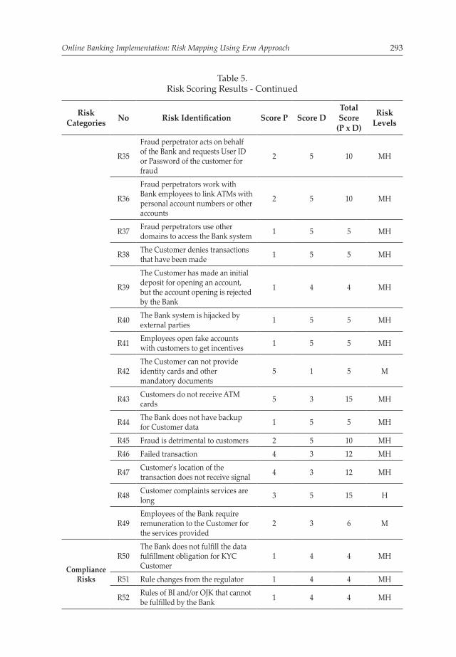
Online Banking Implementation: Risk Mapping Using Erm Approach 293
Table 5.Risk Scoring Results - Continued
Risk Categories No Risk Identification Score P Score D
Total Score
(P x D)
Risk Levels
R35
Fraud perpetrator acts on behalf of the Bank and requests User ID or Password of the customer for fraud
2 5 10 MH
R36
Fraud perpetrators work with Bank employees to link ATMs with personal account numbers or other accounts
2 5 10 MH
R37 Fraud perpetrators use other domains to access the Bank system 1 5 5 MH
R38 The Customer denies transactions that have been made 1 5 5 MH
R39
The Customer has made an initial deposit for opening an account, but the account opening is rejected by the Bank
1 4 4 MH
R40 The Bank system is hijacked by external parties 1 5 5 MH
R41 Employees open fake accounts with customers to get incentives 1 5 5 MH
R42The Customer can not provide identity cards and other mandatory documents
5 1 5 M
R43 Customers do not receive ATM cards 5 3 15 MH
R44 The Bank does not have backup for Customer data 1 5 5 MH
R45 Fraud is detrimental to customers 2 5 10 MHR46 Failed transaction 4 3 12 MH
R47 Customer's location of the transaction does not receive signal 4 3 12 MH
R48 Customer complaints services are long 3 5 15 H
R49Employees of the Bank require remuneration to the Customer for the services provided
2 3 6 M
Compliance Risks
R50The Bank does not fulfill the data fulfillment obligation for KYC Customer
1 4 4 MH
R51 Rule changes from the regulator 1 4 4 MH
R52 Rules of BI and/or OJK that cannot be fulfilled by the Bank 1 4 4 MH

Bulletin of Monetary Economics and Banking, Volume 20, Number 3, January 2018294
Table 5.Risk Scoring Results - Continued
Risk Categories No Risk Identification Score P Score D
Total Score
(P x D)
Risk Levels
Legal Risks
R53 The Bank cannot resolve the dispute with the Customer 1 5 5 MH
R54Lack of clauses in the agreement made by the Bank with the Customer
1 4 4 MH
R55
Changes in the laws and regulations that cause the Bank to change all or part of its agreement with the customer
1 5 5 MH
Source: Bank XYZ processed Data (2016)
Once the risk score results are obtained, we can proceed to make the risk map according to the five risk levels. To make the differentiation easier, the five levels of risk were divided into several colors: High (H) red, Medium to High (MH) orange, Medium (M) yellow, Low to Medium (LM) dark green, and Low (L) green. Figure 1 represents the results of the risk mapping that has been done.
Figure 1. Results of Risk Mapping prior to Mitigation
Negligble (1) Marginal (2) Serious (3) Critical (4) Catastrophic (5)
Frequent(5) R42 R2, R19, R29 R43 R13 R4
Probable(4)
R46, R47
Occasional(3)
R9, R22, R31 R3 R5, R15 R48
Remote(2)
R23 R49 R11 R7, R35, R36,R45
Improbable(1)
R17, R26
R10, R16 R20, R25 R6, R8, R12, R14,
R27, R30, R39, R50, R51, R52,
R54
R1, R18, R21, R24, R28, R32, R33, R34, R37, R38, R40, R41, R44, R53, R55
Source: Processed data of Bank XYZ (2016)
4.5. ERM 5: Risk ResponseBased on the results of the risk mapping that has been done, the risk mitigation measure can be carried out. The identified potential risks are risk mitigation measures so that each risk can be monitored and not shifted towards a higher

Online Banking Implementation: Risk Mapping Using Erm Approach 295
Table 6.Risk Response to the Identified Risks
level of risk. The main priority of the risk mitigation starts with the High-risk level, followed by level Medium to High, Medium, Low to Medium, and finally low-risk level. The risk response to the identified risks, at Bank XYZ, is shown in Table 6.
Risk Category Identified Risks Risk ResponsesLiquidity Risks Banks are bankrupt and customer funds
are non-refundable1. Apply the rules set by BI and OJK,
in particular, the implementation of risk management for liquidity risk.
2. Socialize with the customer on the fact that the Bank's fund is guaranteed by LPS with a maximum amount of 2 Billion Rupiah per customer.
The customer keeps funds in small amount and short term, so the Bank does not get big fund in the long-term
1. Reward the customers who make deposits in certain nominal and a certain period of time.
2. Provide interest rates above the average of the competitors.
Credit Risks The Customer feeling the obligation to pay the loan to the Bank is reduced because it is not directly related to the Bank
1. The Bank shall be required the verification of the customer upon the submission of the loan through a visit to the customer, by telephone, or other media in accordance with BI and/or OJK rules related to KYC (know your customer).
2. Mandatory credit agreement on approved loan. Credit agreements may be sent by mail or email.
The Customer does not make loan payments to the Bank
The Bank sets out the Client's criteria to be granted such as:1. Customer's balance for 6
consecutive months amounts to Rp. 500,000 and above.
2. Make transactions through online banking each month, at least 5 times.
3. Establish the criteria for customer’s job that is eligible for a loan.
Bank does not conduct customer analysis for customer who applies for loan
1. Banks are required to establish rules or policies regarding credit processes that include credit required documents, credit application process, data verification, credit limit, credit approval until the control process must be performed.

Bulletin of Monetary Economics and Banking, Volume 20, Number 3, January 2018296
Table 6.Risk Response to the Identified Risks - Continued
Risk Category Identified Risks Risk Responses2. Banks can collaborate with third
parties to conduct credit score analysis process of the customers applying for loans.
The Bank can not provide customer loan data/information for reporting
1. Fulfill all customer information required under SID rules (debtor information system) in online banking system
2. Storage is required on server or cloud to store customer's data as the whole process is done online.
3. Set the retention period for customer data storage.
Lack of transparency of loan product information to customers, leading to customer complaints
1. The Bank provides a special menu on the online banking display that contains product information in the form of product specifications, costs, and the risks attached to the product.
2. The existence of disclaimer-specific pages prior to the submission of credit sent by the customer containing information that the customer has been given explanation and understand the product he selected.
3. Banks are required to submit credit agreements on loans approved by letter or email from customers.
There is a change of policy from the government/regulator related to credit regulations.
1. The compliance working unit monitors every published government, BI and/or OJK. regulations and reviews the rules
2. Coordinate with work units related to changes in rules such as business, operational, IT, and other units for action.
Market Risks Changes in the value of Rupiah (currency)
1. The risk of changes in the value of Rupiah can be ignored because the current online banking implementation uses the Rupiah as currency.
Changes in interest rates 1. Inform the Customer of interest rate changes through email, SMS, or other media.

Online Banking Implementation: Risk Mapping Using Erm Approach 297
Table 6.Risk Response to the Identified Risks - Continued
Risk Category Identified Risks Risk ResponsesStrategic Risks Fail to achieve product sales target 1. Determine realistic product sales
target according to target market segment.
2. Create tools that contain information on the achievement of sales targets for each sale as material evaluation of target achievement.
Fail to develop products according to customers' needs
1. Analyze the market to determine which market segments to target by utilizing market analytic divisions or using consultant services.
Fail to acquire new customers 1. Conduct promotion through various media, especially social media.
2. Provide promotion by cooperating with store/merchant to offer discount on the purchase certain product.
Fail in prioritizing strategies 1. Set realistic target priorities to be achieved as directed by management. Target priority is submitted along with the timeline/date of its realization.
Competitors get a large market share 1. Provide customer services such as free transaction fee for 50 transactions every month.
2. Offer interest rates above the average of the competitors.
The Bank fails to build an integrated network system with partners
1. Provides 2 network models namely online mode and offline mode. So if the online mode of the system is not running, it will be transferred automatically to offline mode.
Top management that has the capability to provide strategic direction, withdraw from the company
1. Divide the tasks and responsibilities to some senior management. In addition to providing training to employees who are considered to have good potential.
Partner work is not in line with the agreement
1. Make a cooperation agreement (MCC) that contains agreement on the responsibility of both parties, the completion of work, including the steps that must be taken in case of default.

Bulletin of Monetary Economics and Banking, Volume 20, Number 3, January 2018298
Table 6.Risk Response to the Identified Risks - Continued
Risk Category Identified Risks Risk ResponsesOperational Risks Customer can not transact due to
forgotten PIN or User ID1. Provide the User ID/Password
forgot feature on the online banking application and connect it to the email/mobile phone number of the Customer.
The absence of clear procedures and business processes
1. The working units, connected to the online banking process, work together to coordinate the formulation of policies or procedures to develop the operational processes and control those to be run.
The controlling Process of the activities, that have been executed, does not yet exist
1. Standardize rules in the form of Policies or SOPs which contains operational processes that run along with the control process that must be carried out.
Password length/PIN is very complicated 1. Provide PIN / Password reset feature in the online banking application connected with customer's email/phone number.
2. Use biometric authentication in the form of fingerprint scanning or face recognition.
Customer fails to make transactions via ATM
1. Make transaction features, via smartphone, as a key feature in online banking services.
Less effective process 1. Evaluate the process that has been implemented by involving various related units so that more objective input and suggestions can be obtained.
Error in the input data caused by lack of information in the input procedure
1. Create an input procedure that is poured in the form of user manual document.
2. Specify mandatory fields in accordance with BI and/or OJK requirements to be adjusted in the online banking system.
Political situation that leads to riot/demonstration
1. Make transaction features via smartphone as a key feature in online banking services.
Natural disasters on a national scale 1. Make transaction features via smartphone as a key feature in online banking services.

Online Banking Implementation: Risk Mapping Using Erm Approach 299
Table 6.Risk Response to the Identified Risks - Continued
Risk Category Identified Risks Risk Responses2. The security of server/IT devices/
network systems supporting the online banking implementation must be carried out through the Business Continuity Plan (BCP) to keep business processes running.
Theft of Bank information by Customer / Internal Party / External Parties
1. Classify the data into 3 categories which are general, internal, and secret.
2. Restrictions on access to information according to classification based on positions and working units.
3. Standardization of the documents or files naming according to classification.
4. Encrypt if documents or files are sent via email.
The customer can not access the transaction through online banking due to the absence of the network or trouble with the system provider (down)
1. Working with providers with a wide internet network.
2. Provides information to the Customer through display on the Customer's smartphone in relation to the constraints that are being experienced, and directing the Customer to transact through other channels such as ATM.
Bank systems are vulnerable to viruses or malware
1. Periodically update antivirus and firewall.
2. Restrict access to certain web via internet.
3. Restrict access to USB usage on a computer or laptop device.
SMS/Email delivery as transaction proof fails to send
1. Provide proof of transaction notification in online banking feature in the form of transaction history information for the customer.
Fail to store customer data and back it up 1. The need for storage or special storage in the server or cloud to store Customer data in connection with all customer input data carried out online.
2. Set a retention period for customer data storage.

Bulletin of Monetary Economics and Banking, Volume 20, Number 3, January 2018300
Table 6.Risk Response to the Identified Risks - Continued
Risk Category Identified Risks Risk ResponsesTheft of customer user ID by external parties
1. Include information related to the confidentiality of User ID and password at the end of the online banking display when opening an account.
2. Set a password change so that the Customer has to change the password every 3 months.
3. Perform a periodical reminder via SMS or email to the Customer on the need to maintain the confidentiality of the User ID and password.
The fraud perpetrator acts on behalf of the client and unlawfully accesses the customer's account
1. Submitting the authentication code to the Customer's mobile phone for any transactions done by the Customer as a means of verifying the validity of the transaction.
The fraud perpetrator acts on behalf of the Bank and asks the User ID/Password of the customer for fraud
1. Perform a periodical reminder via SMS or email to the Customer on the need to maintain the confidentiality of the User ID and password.
2. Provide harsh sanctions to employees who are proven of committing fraud.
Fraud perpetrators work with Bank employees to link ATMs with personal account numbers or other accounts
1. Apply dual control process (checker and maker) on the linking ATM number process with Customer's account.
2. Provide harsh sanctions to employees who are proven of committing fraud.
Fraud perpetrators use other domains to access the Bank system
1. Restricting system access using only the Bank's internal domains.
The Customer denies transactions that have been made
1. Send the authentication code to the Customer's mobile phone for any transactions done by the Customer as a means of verifying the validity of the transaction.
2. The delivery of transaction evidence by email or SMS.
The Customer has made an initial deposit for opening an account, but the account opening is rejected by the Bank
1. Information is provided that the account opening process, made by the Customer, is semi-active and the Customer will be able to use the account on a regular basis after obtaining approval from the Bank.

Online Banking Implementation: Risk Mapping Using Erm Approach 301
Table 6.Risk Response to the Identified Risks - Continued
Risk Category Identified Risks Risk Responses2. Require the inclusion of column
of account number of destination account for refund in case of account opening decline.
3. Rules are made regarding refund of customer’s funds and their returning SLA to the Customer.
The Bank system is hijacked by external parties
1. The IT Security working unit is required to monitor all system and network security used by the Bank such as performing the vulnerability assessment. Such monitoring shall be conducted periodically.
Employees open fake accounts with customers to get incentives
1. The Bank is required to verify to the Customer upon opening of the proposed account through a visit to the Customer, by telephone, or other media in accordance with BI and/or OJK rules related to KYC (know your customer).
2. Create a direct integration between the Bank system and the Dukcapil system (Population and Civil Registry) to verify the customer data.
The Customer can not provide identity cards and other mandatory documents
1. Create a mandatory document field for the customer so that account opening cannot be processed further if the document is not provided.
Customers do not receive ATM cards 1. Make a notification to the system that the customer has not received yet the ATM card for H + 2 since the opening of Customer's account was approved by Bank.
The Bank does not have backup for Customer data
1. A special storage for customer data back up is required in the server or cloud separated from the core storage.
Reputational Risks
Fraud that is detrimental to customers 1. Provide harsh sanctions to employees who are proven of committing fraud.
2. Socialize all employees regarding the actions of fraud and sanctions.

Bulletin of Monetary Economics and Banking, Volume 20, Number 3, January 2018302
Table 6.Risk Response to the Identified Risks - Continued
Risk Category Identified Risks Risk ResponsesFailed transaction 1. Work with providers that have a
wide internet network.2. Ensure that the infrastructure that
supports online banking services runs well.
3. Compulsory rules must be made when receiving complaints from the Customer, such as the Customer is directed to transact through ATM.
Customer's location of the transaction does not receive signal
1. Work with providers that have a wide internet network.
2. ATM Provides information to the Customer through display on the Customer's smartphone in relation to the constraints that are being experienced, and direct the Customer to transact through other channels such as ATM.
Customer complaints services are long 1. Create a special unit that handles customer complaints.
2. Establish the SLA and inform the customer.
3. Inform the Customer that the complaint service can be reached through the contact center.
Employees of the Bank require remuneration to the Customer for the services provided
1. Provide an appeal to the Client not to provide any kind of compensation to Bank officers through email or SMS media.
2. Provide strict sanctions to Bank officers who are proven to require remuneration from the Customer.
Compliance Risks The Bank does not accomplish the data fulfillment obligation for KYC Customer
1. Ensure that the Bank's system meets all Customer's required information according to KYC (know your customer) rules at the time of account opening.
2. The KYC process is recommended to be performed by a third party with due regard to the rules of BI and/or OJK.
3. The Compliance Work Unit has reviewed the KYC scheme by third parties.
4. Socialization related to KYC process conducted by the third party.

Online Banking Implementation: Risk Mapping Using Erm Approach 303
Table 6.Risk Response to the Identified Risks - Continued
Risk Category Identified Risks Risk ResponsesRule changes from the regulator 1. The Compliance Work Unit
monitors every published government, BI and/or OJK regulations and reviews the rules.
2. Coordinate with work units related to changes in rules such as business, operational, IT, and other units for action.
Rules of BI and/or OJK that cannot be fulfilled by the Bank
1. The Compliance Work Unit reviews the rules of BI and/or OJK and coordinates with relevant work units regarding business process readiness, system readiness, rule readiness, and other infrastructure required to comply with these rules.
Legal Risks The Bank cannot resolve the dispute with the Customer
1. List all of the terms of the relationship between the Bank and the Client including the procedure of settlement in the event of a dispute. All of which are contained in clauses/agreements and approved by the Customer at the opening of online banking.
Lack of clauses in the agreement made by the Bank with the Customer
1. The Legal Work Unit is obliged to review the entire clause of the agreement and ensure all aspects of the agreement have been met.
Changes in laws and regulations that cause the Bank to change all or part of its agreement with the customer
1. The Legal Work Unit monitors every change in published legislation and reviews the rules.
2. Coordinate with work units in relation to changes in rules such as business, operational, IT, and other units for action.
Source: Bank XYZ processed Data (2016)
After the risk mitigation, the process continues with the risk mapping stage which is carried out to obtain an overview of the residual risk. This stage is done through the distribution of questionnaires and in-depth interviews with the parties with competencies in the field of risk and operational processes. The purpose of doing the risk mapping, after mitigation, is to obtain a picture of changes in the risks that occur when the mitigation actions are executed. The risk map, after the risk mitigation process at Bank XYZ, is shown in Figure 2.

Bulletin of Monetary Economics and Banking, Volume 20, Number 3, January 2018304
Figure 2. Results of Risk Mapping Post Mitigation
Negligble (1) Marginal (2) Serious (3) Critical (4) Catastrophic (5)
Frequent(5) R2, R42 R19, R29, R43
R46, R47
R13, R4
Probable(4)
R5, R15
Occasional(3)
R3, R22, R31
R9, R23
Remote(2)
R49 R11 R7, R35, R36, R45 R48
Improbable(1)
R17, R26, R10, R16
R20R6, R8, R12, R14,
R25, R27, R30, R32,R33, R34, R37
R1, R18, R21, R24,R28, R38, R39, R50,
R51, R52, R54 R40, R41, R44,
R53, R55
Sumber: Data Bank XYZ (2016) diolah
Based on the results of risk mapping, after mitigation, it can be seen that there are five potential risks, that previously included the High-risk level, have turned into Medium to High-risk level. However, there are also potential risks that have been mitigated but remain at the same level of risk as before, such as the risk of partner or third party work not in accordance with the agreement. Based on the results of the discussions with respondents, this is due to various factors such as the condition of the partner company experiencing the problem, or the person responsible in the process of withdrawing from the company who took the risk despite mitigation but the risk level has not changed. This level of risk is mandatory for periodic monitoring so that the risk level does not move into higher risk levels.
4.6. ERM 6: Control ActivitiesControl measures are taken to minimize losses incurred by risk and ensure the effectiveness of the responses to risk. Control can be done by Bank XYZ by giving a clear job description for each employee covering specific responsibilities and authorities in the work. The strict monitoring of the implementation of procedures or policies through periodic inspections by the Internal Audit working unit covering all processes should be undertaken along with periodic evaluations of all performance executed in order to address issues or problems arising from the process undertaken which become an important part of the control process.
4.7. ERM 7: Information and CommunicationThe results of the risk assessment that have been undertaken and the risk mitigation advice that has been given must be transmitted and socialized to each related work unit both internal or external to the company, and third-party that is related

Online Banking Implementation: Risk Mapping Using Erm Approach 305
to activities to be followed up so that the potential risk can be controlled. The transmission to the related parties can be in the form of a document procedure or policy or a Cooperation Agreement. In addition, the selection of the communication methods is also important to ensure that the information is delivered. Internal communication methods can be internal meetings using meeting minutes, special portals commonly accessed by employees email. The method of information transmission should also be easy to understand and adequately explained so that each employee understands the information submitted.
4.8. ERM 8: MonitoringAll identified risks must be periodically monitored to keep the risks under control. The supervision can be done through the monitoring of ongoing activities or processes or performing separate evaluations or a combination of both. In addition, there is a need to hold the regular internal meeting to discuss issues or problems arising from the process undertaken. In conducting the monitoring activities, each working unit associated with the process, Internal Audit, along with Risk Management, conducts assessments of various risks, monitors operational activities, and reports the evaluation results to the senior management.
V. CONCLUSIONSThe potential risks identified in the implementation of online banking services are reviewed through eight risk categories established by BI and OJK among as many as 55 potential risks. Strategies applied for effective risk mitigation are more often done for mitigating identified risks. This is done because the online banking business is in the process of development, so the Bank is optimistic about the prospect of online banking business which should still be guided by the rules that apply.
The results of this study are intended to guide in minimizing the emergence of risks through periodic risk control that involves working units related to the online banking process. Furthermore, monitoring, based on the results of customer complaints data and the internal audit of the process undertaken, can be used as the basis for improvement and evaluation in order to monitor other risks that may emerge in the process and were not previously identified.
Implications for the Bank, in connection with the implementation of online banking, in terms of strategic areas i.e. all the company’s strategy to be achieved must be included in a written documents or presentations and socialized to all employees. The operational areas of continuous improvement must be performed through suggestions for innovative and creative process improvement in order to achieve company goals. The reporting field should provide back up data for reporting in relation to some previously unavailable data. Perform data storage or customer information and transaction documents in digital form according to regulatory provisions and retention period of storage. The areas of compliance make sourced policy or procedure in accordance with the applicable law and regulatory regulations. In addition, standardizing the control process for each policy or procedure undertaken with the objective of minimizing the risk posed.

Bulletin of Monetary Economics and Banking, Volume 20, Number 3, January 2018306
REFERENCESBahl, S. (2012). E-Banking: Challenges & Policy Implications. Proceedings of
“I-Society 2012” at GKU, 1–12.Baldwin, A., Shiu, S. (2010). Managing Digital Risk Trends, Issues, and Implications
for Business. (n.d.).Bank Indonesia. (2016). Financial Technology (FinTech) “Analisa Peluang Indonesia
dalam Era Ekonomi Digital dari Aspek Infrastruktur, Teknologi, SDM, dan Regulasi Penyelenggara dan Pendukung Jasa Sistem Pembayaran. Temu Ilmiah Nasional Peneliti 2016 – Kemenkominfo, 1–31
Godfrey. (1996). Control of Risk a Guide to The Systematic Management of Risk from Construction1.pdf. (n.d.).
Cormican, K. (2014). Integrated Enterprise Risk Management : From Process to Best Practice. Modern Economy, (April), 401–413.
COSO-ERM. (2004). Enterprise Risk Management — Integrated Framework, 3(September), 1–16. https://doi.org/10.1504/IJISM.2007.013372
Darmawi. (2006). Manajemen Risiko. Edisi ke-10. Jakarta : Bumi Aksara.Djohanputro, B. (2008). Manajemen Risiko Korporat. Pendidikan dan
Pembinaan Manajemen. Jakarta.Diversitas, K. I. (2008). Tinjauan pustaka, 5–20.Eistert, T., Deighton, J., Marcu, S., Gordon, F., & Ullrich, M. (2013). Banking in a Digital
World. AT Kearney, 23. Retrieved from http://www.atkearney.de/financial-institutions/ideas-insights/featured-article/ /asset_publisher/4rTTGHNzeaaK/content/banking-in-a-digital-world
Ndlovu, I., & Sigola, M. (2013). Benefits and Risks of E-Banking: Case of Commercial Banking In Zimbabwe. The International Journal Of Engineering And Science, 2(4), 34–40. Retrieved from http://www.theijes.com/papers/v2-i4/part. (2)/G0242034040.pdf
Omariba, Z. B., Masese, N. B., & Wanyembi, G. (2012). Security and Privacy of Electronic Banking. International Journal of Computer Science Issues, 9(4), 432–446. Retrieved from http://ijcsi.org/papers/IJCSI-9-4-3-432-446.pdf
Osunmuyiwa, O. (2013). Online Banking and the Risks Involved, 5(2), 50–54.Sarma, G., & Singh, P. K. (2010). Internet Banking : Risk Analysis and Applicability
of Biometric Technology for Authentication. International Journal of Pure and Applied Sciences and Technology, 1(2), 67–78.
Zanoon, N., & Gharaibeh, N. K. (2013). The Impact of Customer Knowledge on the Security of E-Banking. International Journal of Computer Science and Security (IJCSS), 7(2), 81–92. Retrieved from http://www.cscjournals.org/library/manuscriptinfo.php?mc=IJCSS-862

MARKET STRUCTURE AND COMPETITION OFISLAMIC BANKING IN INDONESIA
Sunarmo1
1 Students of Economics and Islamic Finance Specialization, Study Program of the Middle East and Islamic University of Indonesia
The aim of this study is to investigate the market structure and competition of Islamic Banking with H-statistics (Panzar and Roose) model using panel data over a period of July 2010 to September 2014. The result of H-statistics test for long-run equilibrium showed disequilibrium condition. It means that Islamic banking in developing stage. While the market structure and competition test confirmed that the value of the degree of H-statistics generally in monopolistic competition market with score 0.53 to 1.06.
Keywords: equilibrium, structure and competition, Islamic banking in Indonesia, H-statistics (Panzar and Roose model)JEL Classification: C23, D40, D58, G21, L11
ABSTRACT

Bulletin of Monetary Economics and Banking, Volume 20, Number 3, January 2018308
I. INTRODUCTIONThe implementation of the dual banking system, in 2008, stipulated that banks in Indonesia have now embraced two working systems that are based on conventional principles and sharia. A large number of banks will certainly increase banking competition in the country, not to mention the competition in Islamic banking. As of October 2014, there are 13 sharia banks consisting of four foreign exchange banks, six non-foreign exchange banks and three mixed commercial banks (www.ojk.go.id).
The size of competition and the market structure are seen from the market power, which is the ability of a company (seller) to raise its relative price compared to its competitors without losing all its sales. The market power is the difference between the price and the marginal cost expressed relative to the price, which is formulated as L = (P-MC)/P where L is the Lerner index which is an indicator of market power, P is the price at which the firm sells its output, and MC is the company’s marginal cost for the volume of the firm. When P = MC, the firm competes as in perfect competition where the product is sold homogeneously, then L = 0. If P> MC, then L> 0 means that monopolist profit is maximal (Pyndick and Rubinfeld, 2012).
This study uses the company’s share approach on the grounds that this approach is more specific. The theory that can give a clear picture as revealed by Cruch and Ware in Teguh (2013) mentioning that there are two groups of oligopoly companies, namely oligopolies that control some sales or all sales. The first group represents the 8 largest companies that control 75% of the total output in the market. The second represents the 8 companies that control at least 33% of the total market output, if 8 companies control less than 33% of the market share, the industry can be said not concentrated. This statement is supported by Lubis (2012) which uses 8 sample banks in Indonesia.
Based on these two studies, the researcher used samples of 8 sharia commercial banks using the percentage of finance share approach which is the result of the financing amount of each sharia bank proxy to total financing of all sharia banking.
Figure 1. The Rating of Sharia Banks Based on Financing in October 2014 (Processed)
47.78
22.14
9.19 7.614.77 3 2.53 1.74
BankMuamalatIndonesia
Bank SyariahMandiri
Bank RakyatIndonesia
Syariah
Bank PaninSyariah
Bank NegaraIndonesia
Syariah
BankBukopinSyariah
Bank JabarBanten
Bank CentralAsia Syariah

Market Structure and Competition of Islamic Banking in Indonesia 309
Figure 1 showed that the largest percentage of financing is owned by Bank Muamalat Indonesia (47.78%), followed by Bank Syariah Mandiri (22.14%), BRI Syariah (9.19%), Panin Syariah Bank (7.61%), BNI Syariah (4.77%), Bank Bukopin Syariah (3%), and BJB Syariah and BCA Syariah with 2.53% and 1.74%, respectively. The large difference in terms of financing between the top four banks and the four bottom banks indicates that the sharia banking industry is sufficiently concentrated.
The banking concentration will bring competition to some banks, leading to monopoly. Uncompetitive competition is based on structural industry approach i.e. Structure-Conduct-Performance (SCP). The SCP approach assumes a one-way approach between the structure and performance (Martin, 1988). This is a disadvantage of the SCP approach. Thus, a new approach to measuring the competition parameters, based on the behavior, is the New Empirical Industrial Organization (NEIO). One form of this method is the Panzar and Roose model or better-known as the model of H-statistics. Researcher uses this method as it has advantages over other models that are able to determine the broader market structures, estimates using linear regression, simple variables, and the use of individual data (cross section) which is more accurate in predicting market power (Panzar and Roose, 1987). This paper aims to determine both the competition and market structure of sharia banking based on Panzar and Roose parameters.
The second part explores the theories and basic test models. The third section is a research methodology and the fourth section reviews the estimation results. The last part is a conclusion.
II. THEORY2.1. The Development of Sharia BankingThe development of industrial economic calculation was very rapid after the approach of industrial economic model formulated by Bain (1956) through a combination of deductive and empirical approaches. This development has also had an impact on the banking industry. Banks, as strategic institutions in the intermediation of funds, play a significant role in the economic growth. Currently, the banking industry is not only based on the conventional principles, but also on sharia principles. The development of Islamic banking, internationally, was first initiated by Egypt at the Session of the Minister of Foreign Affairs of the Organization of Islamic Conference Organizations (ICO) in Karachi, Pakistan, in December 1970. In subsequent developments in the 1970s, efforts to establish Islamic banks began to spread to many countries. Some countries such as Iran, Pakistan, and Sudan have even transformed their entire financial system into no interest system.
The development of sharia banking continues to the Southeast Asia countries, one of which is Indonesia. The establishment of an Indonesian Islamic bank began in 1980 through discussions on the theme of Islamic banks as pillars of Islamic economy. As a trial, the idea of Islamic banking was practiced on a relatively small scale such as in Bandung (Bait At-Tamwil Salman ITB) and Jakarta (Cooperative Ridho Gusti). Then, in 1990, the Indonesian Ulema Council initiated the

Bulletin of Monetary Economics and Banking, Volume 20, Number 3, January 2018310
establishment of the first Islamic bank, Bank Muamalat Indonesia, which officially operated on May 1, 1992.
Today, the number of sharia banks is increasing due to at least two reasons. Firstly, the crisis of 1998 where Bank Muamalat, in that year, was stronger in facing the crisis. Secondly, Central Bank of Indonesia regulations that have officially implemented dual banking system supported by the enactment of Law Number. 21 of 2008 concerning Sharia Banking.
Both of these causes encouraged the conventional banks to open branches of sharia banks from the initial sharia units, only in the form of development into an independent sharia bank. The increasing number of sharia banks operating in Indonesia certainly pushed the level of competition between banks.
The relevant sizes of banking competition are used i.e. Panzar and Roose models (1987). The usual model, called H statistics, is based on the behavior of individuals or companies in the economy. The PR-H statistic test, in banking, was first performed by Shaffer (1982) with a sample of banks in New York, where the general results of banking in New York operate on monopolistic competition. This is similar to that of Molyneux and Forbes (1995) for banking in Europe, in countries such as France, Germany, Spain, and Britain in the period of 1986-1989, but the banking sector in Italy is indicated as a monopoly market. In addition, many economists such as Panzar and Roose (1987; 1982), Nathan and Neave (1989), Perrakis (1991), Bikker et al (2006) and Goddard and Wilson (2009) recommend the H-statistic PR models. Their study results assumed that companies are free to enter or exit the market without losing capital, and between firms, may lead to competition since it was first established (Gasaymeh, et al, 2014).
2.2. Non-structural approachIf in a structural approach with the SCP model prioritizing one-way approach where the performance of a banking can be seen from its structure, this is certainly not in accordance with the actual conditions in which the banking performance will be more visible from its competing behavior. Then, came the New Empirical Industrial Organization model. The Panzar Roose model, also known as H-Statistics, is an approach commonly used by researchers, especially in the banking industry.
This model was developed by Panzar and Rose in 1987 to measure the degree of competition in an industry, especially banking and competition derivatives in long-term equilibrium, monopoly, and monopolistic competition industries. There are two factors in the acceptance of banking which are the input price and control variable. Assuming that the n - input itself and output production function. The empirical model of H-statistics can be written as follows:
(1)
(2)
where TR is the total revenue, wi as an input factor consisting of wage labor, cost of funds and fixed capital costs. While the CF represents the controlled variable including total capital to total assets and total debt to total assets.

Market Structure and Competition of Islamic Banking in Indonesia 311
The H-statistical value reflects the competitive market structure and is the sum of the elasticity coefficients in the control variables. The representation of the H-statistic values is equal to 0 or negative, then it includes monopolistic competition or collusion oligopoly. It ranges between 0 and 1 for the case of monopolistic competition and if it is 1, then the form of competition is perfect.
The H-statistic model test has different results, it relates to the panel model used whether through Common-Constant, Fixed Effect method or Random Effect method (Naylah, 2010).
Some of the advantages of using H-statistic model are: (1) able to see the broader market structure, (2) can be estimated using linear regression model, (3) only need some variable for testing. Therefore, the Panzar and Roose (PR H-Statistics) model is very comprehensive if used to analyze competition, especially in the banking industry (Panzar and Roose, 1987).
The size of the competition is reflected in the form of market structure. In policy making, banks will consider the form of market structure so that the policy is taken on target. In addition, banks will gain profit or loss based on where they operate. Figure 2 presents the forms of market structure in the economy.
Perfect competition
Imperfect competition
Monopoly
Monopsony
Oligopoly
Oligopsony
Monopolistic
Marketsaccording tostructures
Source: Pindyck and Rubinfeld (2010), processed.
Figure 2. Forms of Markets in Economics
Based on figure 2 above, it can be explained that the perfect competition on the market is an industry where there are many sellers and buyers, and no seller and buyer can influence the price on the market (price taker). Monopoly is a market that has only one seller and many buyers (price maker). Instead, the monopsony market is a market with many sellers but only one buyer. The monopoly and monopsony are closely related. As a sole producer, the position of monopoly is unique. If the monopolist raises the price then he should not worry about competition. This is because the monopolist controls all the output to be sold (Pyndick and Rubinfeld, 2010).

Bulletin of Monetary Economics and Banking, Volume 20, Number 3, January 2018312
The oligopoly market structure is a market structure where few firms compete with one another and the entry of other firms is inhibited, in contrast to the oligopsony which is the market structure with more sellers and more barriers to entry into the market. Basically, the monopolistic market lies between two types of markets namely perfectly competitive market and monopoly market with each company having unique products.
2.3. Empirical Review
Table 1.Summary of Previous H-Statistical Research in The Banking Industry
No Aspects Description1 Author Muhamed Zulkhibri Abdul Majid and Fadzlan Sufian
Title Market Structure and Competition in Emerging Market: Evidence from Malaysian Islamic Banking Industry
Period 2001 – 2005Results H-Statistics ranged between 0.375 - 0.616 while in the equilibrium test the value
ranged between 0824 - 0883 and rejected the Wald test, meaning that the market structure and competition of Islamic banking, in Malaysia, is in the market of monopolistic competition.
2 Author Farhad khodadad Kashi and Jamal Zarein BeynabadiTitle The Degree of Competition in Iranian Banking Industry Panzar – Rosse
ApproachPeriod 2005 – 2010Results H-Statistic of 0.7101, rejecting the Wald test for the monopoly market and
perfect competition with a 1% significance, meaning that the Iranian banks compete in the monopolistic competition market.
3 Author Rima Turk ArissTitle Competitive Condition in Islamic and Conventional Banking: A Global
PerspectivePeriod 2000- 2006Results H statistics showed that the banking in the Middle East operates on
monopolistic market competition and the Lerner index value showed that Islamic banking is more competitive than the conventional.
4 Author Maal NaylahTitle The Influence of Market Structure on the Indonesian Banking PerformancePeriod 2004 – 2008Results Testing of market structure (CR4): oligopolistic form of low moderate
concentration (Type IV)5 Author Andi Fahmi Lubis
Title Indonesian Banking Market Power Period 1990 – 2004 Results Bresnahan-Lau model test showed that the level of competition on the credit
market of Indonesian banking industry is still quite high based on the markup coefficient of 0.0223

Market Structure and Competition of Islamic Banking in Indonesia 313
Table 1.Summary of Previous H-Statistical Research in The Banking Industry (Continued)
No Aspects Description6 Author Anwar Salameh Gasaymeh, Zulkefly A, Mariani Abdul, Mansor Jusoh
Title Competition and Market Structure of Banking Sector: A Panel Study of Jordan and GCC Countries
Period 2003 – 2010 Results The only dynamic Oman model test operates on monopolistic competition,
whereas the Jordan and other GCC countries are in monopolistic competition.7 Author Moh Athoillah
Title Market Structure of the Indonesian Banking Industry: Roose - Panzar TestPeriod 2002 – 2007 Results The condition of the banking market is in the long-term balance and
monopolistic market structure with a value of 0.9318 Author Ratna Sri Widyastuti and Boedi Armanto
Title Competition of the Indonesian Banking IndustryPeriod 2001 – 2006 Results The competition test showed that during the consolidation period, all
commercial banks had monopolistic structure and post API, all banks were on collusive oligopoly market.
9 Author Jean- Michel Sahut, Mehdi Mili, and Maroua Ben KrirTitle Factors of Competitiveness of Islamic Banks in the New Financial OrderPeriod 2000 – 2007 Results Tests of PR-H statistics showed that the Islamic banks (0.0259055) are larger
and significantly competitive than conventional banks (0.006566) and are in the monopolistic market. The Lerner Index test showed that the degree of market power of Islamic banks is (0.8063) greater than that of conventional banks (0.2621)
III. METHODOLOGY3.1. Types and Sources of DataThe data used is panel data which is a combination of individual data (cross-section) and time series data with a sample 8 sharia commercial banks operating in Indonesia and classified based on financing in October 2014 with a time frame between June 2010 - September 2014.
Table 2.Eight Sharia Commercial (C8) Banks
Ranking Sharia Banks 1 Bank Muamalat 2 Bank Syariah Mandiri3 BRI Syariah4 Panin Syariah5 BNI Syariah 6 Bukopin Syariah 7 BJB Syariah 8 BCA Syariah
Source: Financial Statements of Banking Publications, Bank Indonesia and the Financial Services Authority, processed.

Bulletin of Monetary Economics and Banking, Volume 20, Number 3, January 2018314
3.2. Variable RestrictionsThe variables consist of three independent variables, including labor inputs, cost of funds, fixed capital cost, and two controlled variables i.e. primary ratio, the asset to loan ratio, while the dependent variable uses the income ratio and return on asset (ROA).
Table 3.PR-H Statistic Variables
Names of Data Types of Variables Time Frame Units of
Measurement Sources of
DataTotal Revenue (TR) Bound Monthly Ratio BI and FSAReturn on Asset (ROA) Bound Monthly Ratio BI and FSAWages of labor (WL) Free Monthly Ratio BI and FSACost of funds (WF) Free Monthly Ratio BI and FSAFixed capital costs (WK) Free Monthly Ratio BI and FSAPrimary ratio (Y1) Free Monthly Ratio BI and FSAAsset to loan ratio (Y2) Free Monthly Ratio BI and FSA
Description of variable constraints:1. Total revenue (TR) is total bank income derived from non-interest operational
income for sharia banking which is proxy to total asset2. Return on Assets (ROA) is the ability of a bank to make the profit through the
use of its assets. The ROA is in proxy from the profit before tax to total assets3. Wages of Labor (WL) is the operational cost of the bank in terms of labor wages.
The wage of labor is the burden the bank must pay to its workers. It uses the ratio of wages to total assets
4. The cost of funds (WF) is the burden borne by banks for bonuses on third parties (customers)
5. The Fixed capital cost (WK) is an administrative and promotional burden to be borne by a bank that is proxied using owned assets.
6. The Primary ratio (Y1) is a ratio of capital health which measures the extent to which the decrease in total incoming assets can be covered by capital
7. The asset to loan ratio (Y2) is the ratio to measure the amount of financing disbursed by the total assets owned by sharia banks.
3.3. Models and Methods of AnalysisData analysis is the process of simplifying the data into a form that is easier to read and interpret. The econometric model for panel data was used in the present research. The form of the equation was as follows:
Yit = β0 + β1X1it + β2X2it + β3X3it + βnX3it + εit (3)
The stages of panel data test consist of Pooled Least Square modeling, Fixed Effect, and Random Effect.

Market Structure and Competition of Islamic Banking in Indonesia 315
3.4. PR H-Statistic MethodThe PR H-statistic method is one form of market power measurement in the banking industry with the un-structural approach. The un-structural approach is more of determining the company’s behavioral aspects in influencing the market conditions (Widyastuti and Armanto, 2013). This method was first developed by Panzar and Roose in 1987 and used to measure the degree of market power in the banking industry. The measure of market power through the PR H-statistics is derived from the sum of the input of price elasticity coefficients i.e. labor costs (WL), cost of funds (WF) and fixed capital costs (WK), which respond to the total revenue. The representation of the sum of input variables can be used to determine the market structure in which the firm operates.
Some of the advantages of the PR H-statistic method are: (1) able to see the broader market structure, (2) can be estimated using econometric model with regression, (3) the variable used is quite simple, (4) using the individual data (cross-section) as a form of competition among banks.
The PR-H Statistics method is applied to companies with one type of product. Thus, banks are treated as producers with output in the form of loans. The assumptions of this method are long-run equilibrium and the maximization of profit earning (Panzar and Roose, 1987).
Before estimating the PR H-statistic, a long-run equilibrium test is intended, for, in case of balance, the research can proceed to market power, whereas if not, the research is stopped. However, Shaffer (1985) in Widyastuti and Armanto (2013), said that if the study shows a disequilibrium condition, it indicates that the banking industry is developing dynamically during research observation, thus, the research can proceed.
The equation of long-run equilibrium test of the PR-H statistic method is as follows:
LnROAit = β 0 + β1Ln(WL,it)+ β2Ln(WF,it) + β3 Ln(WK,it) + β4Ln( Y1,it)+ β5Ln(Y2,it) + εit (4)
The long-run equilibrium is interpreted as follows: If PR - H statisticROA < 0 there is no equilibriumIf PR – H statisticROA = 0 there is equilibriumPR – H statisticROA is the sum of the elasticities of β1, β2, and β3. Whereas, the equation to see the degree of market power is only by replacing the variable Return on Asset (ROA) with total bank income to total assets (TR).
So, the equation becomes:
Ln(TRit) = β 0 + β1Ln(WL,it)+ β 2Ln(WF,it) + β3 Ln(WK,it) + β4Ln( Y1,it)+ β5Ln(Y2,it) + εit (5)
Description:lnTRit = Non-interest income/total assets lnROAit = Profit before tax/total assetslnWF,it = Bonus expense (wadiah)/total assets lnWL,it = Labor load/ total assets

Bulletin of Monetary Economics and Banking, Volume 20, Number 3, January 2018316
lnWK,it = Operational load/total assets lnY1,it = Total capital/total assetslnY2,it = Total debt/total assetsThe interpretation of the market power is as follows.PR-H statisticTR = 0 monopolistic competitionPR-H statisticTR = 1 perfect competitionPR-H statisticTR 0 < HTR < 1 = Monopolistic Competition
All of the variables in the PR H-statistic method use the addition of natural logarithm (ln) to show elasticity, since the market power values range between 0 and 1 so that the degree of the market indicator is immediately detected.
IV. RESULTS AND ANALYSIS4.1. Panzar and Roose (PR H- Statistics) analysisThe panel data estimation is done on Eviews 7 with the timeframe of July 2010-September 2014, which is grouped every 3 months. Thus, there are 17 test result data of test phase, consisting of the best method selection (PLS, FEM, or REM), equilibrium test, and PR H-Statistic test. The results and discussion of each test are described as follows.
4.2. The Best Model of Sharia Bank Equilibrium Test
Table 4.Selection of The Best Model of Sharia Bank Equilibrium Test
Periods TestModel Selection
Prob Significance 0.05 Best Model Conclusion
July – September 2010
ChowHousman
0.00000.0507
0.050.05
FEMREM
The best model is REM, because 0.0507 > 0.05
October – December 2010
ChowHousman
0.00000.0000
0.050.05
FEMFEM
The best model is FEM, because 0.0000 < 0.05
January – March 2011
ChowHousman
0.00000.3875
0.050.05
FEMREM
The best model is REM, because 0.3875 > 0.05
April – June 2011
ChowHousman
0.00000.0320
0.050.05
FEMFEM
The best model is FEM, because 0.0320 < 0.05
July – September 2011
ChowHousman
0.00000.0479
0.050.05
FEMFEM
The best model is FEM, because 0.0479 < 0.05
October – December 2011
ChowHousman
0.00000.9381
0.050.05
FEMREM
The best model is REM, because 0.9381 > 0.05
January – March 2012
ChowHousman
0.00010.9839
0.050.05
FEMREM
The best model is REM, because 0.9839 > 0.05

Market Structure and Competition of Islamic Banking in Indonesia 317
Periods TestModel Selection
Prob Significance 0.05 Best Model Conclusion
April – June 2012
ChowHousman
0.00000.8299
0.050.05
FEMREM
The best model is REM because 0.82>0.05
July – September 2012
ChowHousman
0.00000.0000
0.050.05
FEMFEM
The best model is FEM, because 0.0000 < 0.05
October – December 2012
ChowHousman
0.00000.4376
0.050.05
FEMREM
The best model is REM, because 0.4376 > 0.05
January – March 2013
ChowHousman
0.00000.0000
0.050.05
FEMFEM
The best model is REM, because 0.0000 < 0.05
April – June 2013
ChowHousman
0.00280.8007
0.050.05
FEMREM
The best model is REM, because 0.8007 < 0.05
July – September 2013
ChowHousman
0.00000.5859
0.050.05
FEMREM
The best model is REM, because 0.5859 > 0.05
October – December 2013
ChowHousman
0.00000.2848
0.050.05
FEMREM
The best model is REM, because 0.2848 > 0.05
January – March 2014
ChowHousman
0.00000.6506
0.050.05
FEMREM
The best model is REM, because 0.6506 > 0.05
April – June 2014
ChowHousman
0.00000.7878
0.050.05
FEMREM
The best model is REM, because 0.7878 > 0.05
July – September 2014
ChowHousman
0.00000.8698
0.050.05
FEMREM
The best model is REM, because 0.8698 > 0.05
Source: Appendix 2.
Table 4.Selection of The Best Model of Sharia Bank Equilibrium Test (Continued)
The selection of the best model for sharia bank equilibrium test, as in Table 12, is Fixed effect model and Random Effect Model (REM). The FEM modeling took place in the period of October-December 2010, April-June 2011, July-September 2011, July-September 2012, and January-March 2013, while the other twelve periods used the REM test. However, this test often raises the problem of correlation between interference variables (autocorrelation), and to overcome it, the REM test method of Generalized Least Square (GLS) is used.

Bulletin of Monetary Economics and Banking, Volume 20, Number 3, January 2018318
4.3. Best Model of PR H-Statistics Test in Sharia Banking
Table 5.Selection of The Best Models of PR H-Statistics Test in Sharia Banking
Periods TestPemilihan Model
Prob Significance 0,05 Best model Conclusion
July – September 2010
ChowHousman
0.00000.3360
0.050.05
FEMREM
The best model is REM, because 0.3360 > 0.05
October – December 2010
ChowHousman
0.00000.7003
0.050.05
FEMREM
The best model is REM, because 0.7003 > 0.05
January – March 2011
ChowHousman
0.00000.0201
0.050.05
FEMFEM
The best model is FEM, because 0.0201 < 0.05
April – June 2011
ChowHousman
0.00000.0044
0.050.05
FEMFEM
The best model is FEM, because 0.0044 < 0.05
July – September 2011
ChowHousman
0.00000.0048
0.050.05
FEMFEM
The best model is FEM, because 0.0048 < 0.05
October – December 2011
Chow 0.0005 0.05 FEM The best model is REM, because 0.5280 > 0.05
January – March 2012
HousmanChow
0.52800.0001
0.050.05
REMFEM
The best model is REM, because 0.1144 > 0.05
April – June 2012
HousmanChow
0.11440.0001
0.050.05
REMFEM
The best model is FEM, because 0.0000 < 0.05
July – September 2012
ChowHousman
0.00000.0000
0.050.05
FEMFEM
The best model is FEM, because 0.0000 < 0.05
October – December 2012
ChowHousman
0.00020.6590
0.050.05
FEMREM
The best model is REM, because 0.6590 > 0.05
January – March 2013
ChowHousman
0.00000.0000
0.050.05
FEMFEM
The best model is REM, because 0.0000 < 0.05
April – June 2013
ChowHousman
0.00000.0015
0.050.05
FEMFEM
The best model is FEM, because 0.0015 < 0.05
July – September 2013
ChowHousman
0.00000.0000
0.050.05
FEMFEM
The best model is REM, because 0.0000 < 0.05
October – December 2013
Chow 0.4769 0.05 PLS The best model is PLS, because 0.4769 > 0.05
January – March 2014
ChowHousman
0.00000.0000
0.050.05
FEMFEM
The best model is FEM, because 0.0000 < 0.05

Market Structure and Competition of Islamic Banking in Indonesia 319
Table 5.Selection of Best Models of PR H-Statistics Test in Sharia Banking (Continued)
Periods TestPemilihan Model
Prob Significance 0,05 Best model Conclusion
April – June 2014
ChowHousman
0.00000.0000
0.050.05
FEMFEM
The best model is FEM, because 0.0000 < 0.05
July – September 2014
ChowHousman
0.00000.0000
0.050.05
FEMFEM
The best model is FEM, because 0.0000 < 0.05
Source:
In general, in Table 14, the best model used in the estimation of the PR-H statistics sharia banking is the Fixed Effect Model (FEM) of 11 periods, while the Random effect is 5 periods i.e. July-September 2010, October-December 2010, October-December 2011, January-March 2012, and October-December 2012. Meanwhile, the Pooled Least Square model (PLS) is used in the period of October-December 2013. The PLS modeling, in that period, shows that the eight-sharia banking is assumed to have the same intercept and slope.
4.4. Long Run Equilibrium Test Results of Sharia BankingThis test is used to view the long-run equilibrium and is the sum of the input variable coefficients of the estimation using the Eviews 6.0 i.e. labor cost (InWL), cost of funds (InWF), and capital cost (InWK) which are the main requirements of continuing to H - Statistics.
Figure 3. The Result of Long-Run Equilibrium Test of Sharia Banking, from July–September 2010 to July–September 2014
-1
-0.5
0
0.5
1
1.5
2
Jul -Sep
Okt -Des
Jan -Mar
Apr -Jun
Jul -Sep
Okt -Des
Jan -Mar
Apr -Jun
Jul -Sep
Okt -Des
Jan -Mar
Apr -Jun
Jul -Sep
Okt -Des
Jan -Mar
Apr -Jun
Jul -Sep
2010 2011 2012 2013 2014
-0.74
0.32 0.4
1.021.16
-0.86
0.64
0.27
1.43
0.82
1.1
0.5 0.58 0.650.78
-0.47
1.64

Bulletin of Monetary Economics and Banking, Volume 20, Number 3, January 2018320
Sharia banking appears to have a tendency to approach the equilibrium level indicated by the value close to 0. However, the movement is quite extreme in the period of July-September with (1.16 points), July-September 2012 (1.43 points), and July-September 2014 (1.64 points).
Sharia banking is in disequilibrium condition and tends to approach 0. This is similar to the research conducted by Widyastuti and Armanto (2013) and Sahut, et al. (2012).
This condition indicates that sharia banking is in a developing condition which means that sharia banking is not yet dominating the economy. This is in line with the Financial Services Authority survey in 2013 on financial literacy, which showed that the community’s understanding of banking was only 21.80%, which was lower compared to the Philippines (27%), Malaysia (66%), Thailand (73%) and Singapore with the highest level of understanding of the banking sector i.e. 98%.
The low level of banking literacy, in Indonesia, indicates that many people do not use banking as a financial intermediary institution. This has an impact on the low DPK owned by sharia banks and the hampering growth of the real sector.
The continuous development of sharia banking, in Indonesia, is caused by the visibility of its new market share of about 5% of the total banking assets in Indonesia. So, it takes hard work to add customers. One of the efforts made by the Financial Services Authority and Bank Indonesia is the promotion of Islamic finance, policy-making, and legislation. However, their efforts are certainly not enough to increase the market share of sharia banking. Therefore, there is a need for the role of the banking itself and the community. The efforts that need to be done by sharia banking is the increase in the number of branches and ATMs in the regions. In 2017, FSA recorded the number of operational headquarters (KPO) of sharia banks as follows: 152 offices, 136 sub-branches and 53 cash offices (still lacking).
Another effort that can be carried out is through the role of ulama in providing education on Islamic finance through Islamic study materials in mosques. With the collaboration of the government, banks, and community, it is expected that the future of sharia banking will be more advanced, growing and stable.

Market Structure and Competition of Islamic Banking in Indonesia 321
4.5. PR H-Statistics Test Results of Sharia Banking
Figure 4. PR H-Statistics Results Conventional and Sharia Bankingfrom July-September 2010 to July-September 2014
Jul -Sep
Okt -Des
Jan -Mar
Apr -Jun
Jul -Sep
Okt -Des
Jan -Mar
Apr -Jun
Jul -Sep
Okt -Des
Jan -Mar
Apr -Jun
Jul -Sep
Okt -Des
Jan -Mar
Apr -Jun
Jul -Sep
2010 2011 2012 2013 2014
0
0.2
0.4
0.6
0.8
1
1.2H-statistic parameter
Figure 4 shows that the pattern of the strength of sharia banking always falls within a range of more than 0 to more than 1, indicating that it is in the perfect market and monopolistic competitions.
Perfect competition conditions occur twice i.e. in the period of July-September 2013 (1.05) and July-September 2014 (1.06). Meanwhile, the other periods operate in the monopolistic market. This means that the diversity of products and advertising in sharia banking during this period is quite dominant in order to increase the number of customers. The strong competition amongst sharia banks is caused by the dominance of conventional banking that opened the branch of sharia after the endurance of Bank Muamalat Indonesia during the economic crisis of 1998 (Faiz, 2010).
Another factor is the regulation of the Ministry of Religious Affairs of the Republic of Indonesia related to the pilgrimage funds that must be deposited into Islamic banking, which reflect the government’s trust in Islamic banks in the management of pilgrim funds. In addition, sharia state securities products (retail Sukuk) issued by the government was recently quite enthused by the community. However, the products of Islamic banks themselves, in practice, are still dominated by the sale and purchase agreement (Murabaha) (Natadipurba, 2015).
Generally present in a monopolistic market and perfect competition means that although the product differentiation is quite good, there is still a perfect competition condition. This shows that sharia banking has not been consistent in making innovative financial products. Therefore, in the future, shariah banking needs to make superior financial products that will become his trademark. Thus, each sharia bank has its own market share and can compete from the non-price side.

Bulletin of Monetary Economics and Banking, Volume 20, Number 3, January 2018322
V. CONCLUSIONS5.1. Conclusions Based on the description and discussion, it can be concluded that:1. The equilibrium test results show the value close to 0, meaning that the
condition of sharia banking, in the long run, does not show equilibrium. This means that sharia banking is in a developing condition. Therefore, the collaboration between the government, especially FSA and BI, banking and community is needed to increase the growth of sharia banking in the future.
2. The H-statistic test results show that sharia banking operates on the monopolistic market and perfect competition. This means that sharia banking has not been consistent in developing its products. So, it requires the development of excellent products with specific characteristics and market share.
5.2. SuggestionsThe suggestions submitted by the author for further research improvements are as follows:1. In order for the results to be more comprehensive, there is a need for additional
variables and period of study.2. The high level of competition in sharia banking demands the government, in
this case, the Financial Services Authority and related parties, to improve the level of interbank competition.
REFERENCESAl-Obaidin, A.M. (2008). Market Structure, Concentration and Performance in
the Commercial Banking Industry of Emerging Markets Eropean. Journal of Economics, Finance and Administrative Science. No. 12:104 – 115.
Ariss, Rima Turk. (2010). Competitive Condition in Islamic and Conventional Banking : A Global Perspective. Journal Review of Financial Economics.
Athoillah, Moh. (2010). Struktur Pasar Industri Perbankan Indonesia: Rosse – Panzar Test. Journal of Indonesian Applied Economics.
Badan Pusat Statistik Republik Indonesia. from www. BPS.go.id.Berger, Demirguc-Kunt, Levine, N and Haubrich, J. (2004). Bank Concentration
and Competition: An Evolution in the Making. Global Perspective. Journal of Money,Credit, and Banking.
Billas, A. Richard. (1985). Microeconomic Theory. Second Edition. McGraw-Hill Book Company. Singapore.
Bisnis. (2014). Retrieved July, 2015, from www.bisnis.com.Carlton, Dennis and Perloff, Jeffrey. (2006). Modern Industrial Organization. Fourth
Edition. Addison Wesley. USA.Faiz, Ihda. (2010). Ketahanan Kredit Perbankan Syariah Terhadap Krisis Keuangan
Global. Jurnal Ekonomi Islam La_Riba. Vol. IV no.2. Gasaymeh, A, Karim Abdul Z, dkk. (2014). Competition and Market Structure
of Banking Sector: A Panel Study of Jordan and Gulf Council Cooperation Countries (GCC). Jurnal Ekonomi Malaysia. 48: 23- 24.
Market Structure and Competition of Islamic Banking in Indonesia 323
Gujarati, Damodar. (2007). Dasar – Dasar Ekonometrika Jilid 1 Edisi 3. Erlangga. Jakarta.
Hasibuan, Nurimansyah. (1993). Ekonomi Industri: Persaingan,Monopoli dan Regulasi. LP3ES. Yogyakarta.
Otoritas Jasa Keuangan. (2017). Retrieved October, 2017, from http://www.ojk.go.id/id/kanal/syariah/tentang-syariah/Pages/Sejarah-Perbankan-Syariah.aspx.
Howe, Stewart. (1978). Industrial Economics: An Applied Approach. The Macmillan Press LTD. USA.
Infobank. (2014). Retrieved Januari, 2014, from http://www.infobank.com.Ismail. (2010). Manajemen Perbankan dari Teori Menuju Aplikasi. Kencana Prenada
Media Grup. Jakarta.Kashi dan Jamal. (2013). The Degree of Competition in Iranian Banking Industry
Panzar – Rosse Approach.African Journal of Management. Vol.7(43).pp.4380 – 4385.
Kompas online.(2014). bisniskeuangankompas.com. Diakses Juli 2015.Kontan online. (2014). Retrieved Juli 2015, from http//www.keuangan.kontan.co.idBank Indonesia. Laporan Keuangan Publikasi Bank. from http://www.bi.go.id.Otoritas Jasa Keuangan. Laporan Keuangan Publikasi Bank. from http://www.ojk.
go.id. Lubis, Fahmi Andi. (2012). Market Power Perbankan Indonesia. Buletin Ekonomi
Moneter dan Perbankan Bank Indonesia. Mankiw,N. Gregory. (2009). Macroeconomic. Seventh Edition. Worth Publisher. USA.Molyneux, P. dan Forbes, W. (1995). Market Structure and Performance in Eropean
Banking. Applied Economics. 27: 155 – 159.Natadipurba, Chandra. (2015). Ekonomi Islam 101. Bandung : Mobidelta Indonesia.Naylah, Maal. (2010). Pengaruh Struktur Pasar Terhadap Kinerja Perbankan
Indonesia. (Tesis). Universitas Diponegoro. Semarang.Panzar, J. and Roose, J. (1987). Testing for Monopoly Equilibrium. Journal of
Industrial Economics. Pindyck and Rubinfeld. (2010). Mikroekonomi. Edisi Keenam. Jilid 2. Jakarta: Indeks. Pindyck and Rubinfeld. (2012). Mikroekonomi. Edisi Kedelapan. Jilid 1. Jakarta:
Erlangga. Rosadi,Dedi. (2012). Ekonometrika dan Analisis Runtun Waktu Terapan dengan Eviews.
Yogyakarta : CV Andi Offset.Sahut Michel, Mili Mehdi, Krir Ben. (2012). Factors of Competitiveness of Islamic
Banks in the New Financial Order. 8th International Conference on Islamic Economics and Finance.
Shaffer, S. (1982). A Non – Structural Test for Competition in Financial Markets. Bank Structure and Competition, Conference Proccedings. 225 – 224.
Silalahi, Ulber. (2009). Metode Penelitian Sosial. Jakarta : Refika Aditama.Smirlock, M.(1985). Evidence on the (Non) Relationship Between Concentration
and Profitability in Banking . Journal of Money, Credit and Banking. Vol 17, No.1:69 -83
Stigler, J, George. (1947). The Kinked Oligopoly Demand Curve and Rigid Price. USA : Homewood – Illinous.

Bulletin of Monetary Economics and Banking, Volume 20, Number 3, January 2018324
Subandi,Ghozali Imam. (2013). Determinan Efisiensi dan Dampaknya Terhadap Kinerja Profitabilitas Industri Perbankan di Indonesia. Jurnal Keuangan dan Perbankan. 17: 123 – 135.
Sukirno, Sadono. (2010). Mikro Ekonomi Teori Pengantar. Edisi Ketiga. Jakarta : Raja Grafindo Persada.
Suliyanto. (2011). Ekonometrika Terapan: Teori dan Aplikasi dengan SPSS. Yogyakarta : Andi Offset
Taswan. (2010). Manajemen Perbankan Konsep, Teknik & Aplikasi. Yogyakarta : UPP STIM YKPN.
Teguh, Muhammad.(2013). Ekonomi Industri. Jakarta : RajaGrafindo Persada. Undang – Undang Nomor 21 tahun 2011 tentang Otoritas Jasa KeuanganUniversitas Lampung. (2011). Format Penulisan Karya Ilmiah Universitas Lampung.
Penerbit Universitas Lampung. Bandar Lampung.Widarjono, Agus. (2009). Ekonometrika Pengantar dan Aplikasinya. Edisi Ketiga.
Yogyakarta. Ekonusia. Widyastuti, Sri. R dan Armanto, Boedi. (2013). Kompetisi Industri Perbankan
Indonesia. Buletin Ekonomi Moneter dan Perbankan Bank Indonesia. Zulkhibri.et.al. (2007). Market Structure and Competition in Emerging Market:
Evidence from Malaysian Islamic Banking Industry.MPRA Paper No.12126
ANNS-BASED EARLY WARNING SYSTEM FORINDONESIAN ISLAMIC BANKS
Saiful Anwar1, A.M. Hasan Ali2
1. Lecturer at STIE Ahmad Dahlan, Jakarta and Risk Oversight Committee, PT. Bank BRI Syariah. Email: [email protected]. Lecturer at UIN Syarif Hidayatullah, Jakarta Email: [email protected]
This research proposes a development of Early Warning System (EWS) model towards the financial performance of Islamic bank using financial ratios and macroeconomic indicators. The result of this paper is ready-to-use algorithm for the issue that needs to be solved shortly using machine learning technique which is not widely applied in Islamic banking. The research was conducted in three stages using Artificial Neural Networks (ANNs) technique: the selection of variables that significantly affect financial performance, developing an algorithm as a predictor and testing the predictor algorithm using out of sample data. Finally, the research concludes that the proposed model results in 100% accuracy for predicting Islamic bank’s financial conditions for the next two consecutive months.
Keywords: Early Warning System, Artificial Neural Networks, Islamic Banks, Financial Distress.JEL Classification: C45, C53, G33, G21
ABSTRACT

Bulletin of Monetary Economics and Banking, Volume 20, Number 3, January 2018326
I. INTRODUCTION The golden period experienced by Islamic banks has apparently been passed. The growth over 20% per year that occurred in 2009 until 2011 is continuously experiencing a decreasing trend. In 2012, Indonesian Central Bank reported that the growth of market shares of Islamic banks doubly decreased to 9.44% and further experienced a negative trend with a growth rate of 6.07% in 2013. Finally, for the first time in Indonesian Islamic Bank’s development period, the market shares of Islamic banks experienced a negative growth of 4% in December 2014. The year actually became a difficult year for Islamic banking due to the increase of interest rate which caused the cost of bank funds to soar. In the first semester of 2013, the SBI interest rate stood still at 5.75% which was then kept increasing towards 7.75% in October 2014. This growth rate had a direct impact on the increase of deposit rates of conventional banks as the competitors of Islamic banks in collecting third-party funds. At the end of 2014, one of the Islamic banks offered a profit sharing rate for its deposit products which was equivalent to 10%-11% of interest rate in order to compete with conventional banks which offered averagely 8.07% in the same period for the one month of deposit. The significant pressure on the cost of funds affected the growth rate of market shares of Islamic banking decreasing. The profit of Islamic bank grew only 15.1% in 2014 compared with previous year which successfully reached 43.8% growth. The hard pressure towards Islamic bank’s profit was triggered not only by the weakening of national economy marked by high inflation and the continuously weakening exchange rate but also due to the weakness of the Good Corporate Governance of Islamic banks.
The Non-Performing Financing (NPF) ratio of Islamic banks at the end of 2014 reached 4.33%, a very significant increase compared with the previous period which was only 2.62%. The more worrying conditions will be more clear when looking more detail at the absolute amount of NPF, whereas the default financing category increased to 2.24%, amounted to Rp4.465 trillion. This is almost equal to the total amount of NPF in 2013 which amounted to Rp4.828 trillion. This condition got worse with the widespread news of fraud occurred in the biggest Islamic bank in Indonesia which loosed hundreds of billions of rupiahs, causing the increase of reputational risk for Islamic banking industry.
The condition has created excessive distressing which comes from the social and economic views. The excessive distressing appears since the Islamic banking industry employs around 42 thousand employees which their lives and families’ welfare depend on. Additionally, it would decline the derivative industries such as education whereas thousands of schools and universities already offered Islamic finance subject and already attracted tens of thousands of students throughout Indonesia. The social turbulence with significant economic loss will surely happen when a particular Islamic bank experiences difficulty. This local problem could be spread out which then created systemic risk.
Further, the systemic risk in Islamic bank could degrade the reputation of Islamic bank as a type of business institution which uses the symbol of religion. This could be a boomerang for Islamic economic development wherein intensive socialization has been conducted about the fact that the Islamic economy with its financing instruments is thought as an alternative financing system. The system is expected to become a catalyst for economic fluctuations due to maysir (gambling), ghoror (speculation), and riba (interest) transaction (Chapra, 2009).

Anns-Based Early Warning System for Indonesian Islamic Banks 327
Financial Services Authority (OJK) Act number 21 of 2011, the institution is mandated to organize a system of regulation and supervision which is integrated towards the entirety of activities in the financial services sector as to create a financial system condition which is organized, fair, transparent, and accountable, as well as to grow in a sustainable and stable way so that it is able to protect consumer and public interests. Accordingly, OJK has a responsibility to conduct preventive actions, one of which is to develop early warning system (EWS) for Islamic bank’s failure detection. According to Indonesian, The EWS works to perform monitoring and supervision by providing signals indicating the probability of a declining in a bank’s performance. According to that signals, the OJK can determine which banks are necessary to get strict supervision and give aid in a short time in the form of financing or managerial supervision to immediately pulled out the bank from bad conditions that probably lead towards bankruptcy.
Othman (2012) reveals that financial authority has two methods to develop EWS which are an on-site examination and off-site examination methods. The prior method is conducted by performing a direct assessment on the day to day banking operation. Pettway and Sinkey (1980) suggest EWS using accounting data and market information to determine the priority of the banks which need an on-site examination. Meanwhile, the off-site examination is a statistics or mathematics based method to determine the probability of a bank’s bankruptcy (Othman, 2012). The effectivity of this method is measured according to its accuracy in classifying whether a particular bank is in a troubled or not compared to its actual condition.
Beaver (1966) is the first researcher who makes prediction using Univariate Discriminant Analysis method to make a prediction of bankruptcy. Two years after that, Altman (1968) introduced a model to predict a company’s bankruptcy using Multiple-Discriminant Analysis (MDA) method which is now widely known as the Altman Z-score. In the 1980s, Takahashi (1984) and Friedmen et al. (1985) utilized the Recursive Partitioning Algorithm to predict bankruptcy. Bellovary et al. (2007) applied the statistical method and mathematical models to make a prediction. He observed many statistical and mathematical method starting from a simple statistical method until a complex data mining method such as neural networks.
Bellovary et al. (2007) reported that the use of the statistical method and data mining technique which introduced since year 1990s, resulted in a wide variety of accuracy. He observed 106 researchers who use statistical methods resulted in accuracy rate ranging from 24% to 94% in predicting a company’s bankruptcy. Moreover, 40 researchers who use data mining techniques such as neural network resulted in accuracy rate ranging from 71% to 100%. Liao et al. (2012) reported that the usage of data mining technique received more attention since the number of the researcher who uses the technique is rapidly growing. The technique has many types such as artificial neural network, clustering, association rule, artificial intelligence, bioinformatics, fuzzy logic, support vector machine and so forth. Particularly, for the case of Indonesian Islamic bank research, Anwar and Ismal (2011) reported that the artificial neural network method empirically possesses a higher accuracy rate compared to support vector machine method in predicting the profit sharing rate of Islamic banks in Indonesia. The result depicted that the artificial neural network model has a better ability in understanding the context of the diversity and volatility of data patterns.
Bulletin of Monetary Economics and Banking, Volume 20, Number 3, January 2018328
Accordingly, this research summarizes problems associated with Indonesian Islamic bank’s performance that is necessary to solve, which are:1. The decreasing of the financial performance of Islamic banks is considered to
be main cause why many targets proclaimed by OJK are failed to be achieved such as the percentage of market share and profitability ratios.
2. The uniqueness of operational and business model of Islamic banks which lead to the special risks that are not found in conventional banks, such as displaced commercial risk and investment risk.
3. The very volatile economic conditions, such as the instability of exchange rates which causes the disturbance on achieving the growth rate targeted through the rise of credit risk and the liquidity problem in money market which creates difficulty to Islamic banks in obtaining a low cost of fund.Therefore, it is necessary for Islamic banks to have EWS signaling the decreasing
of financial performance. The EWS must be suitable with the characteristics and uniqueness of Islamic banks, ultimately in determining the best algorithms that understand those conditions properly. In order to answer the problems, the development of an EWS model is highly needed. For that purpose, this research will attempt to explore, to empirically test and to analyze as many as possible the reason for performance decrease in Islamic bank guided by research questions below:1. What kind of variables could give negative impact to financial performance of
Islamic banks?2. How accurate are artificial neural networks (ANNs) as prediction algorithm in
making a prediction (in term of accuracy)?This research will use Bank Syariah Mandiri, the biggest Islamic bank in
Indonesia, as a case study in measuring the accuracy and stability of ANNs as a prediction algorithm in EWS
II. THEORY 2.1. Financial DistressThe term of systemic risk is defined as the probability of severity that would affect other banks when a bank experiences problems. In another word, when a bank faces a financial decrease, it would possibly trigger financial decrease to other banks and at the end, the entire industry could be collapsed. This is why financial problems in a bank will frighten other parties and the economic system as a whole (Othman, 2012).
The financial problem was discussed by Altman (1993) who differentiated the conditions of a company’s financial condition into four types: failure, insolvency, default, and bankruptcy. In detail, failure is a condition where the rate of return of money invested experiences a continuous decreasing which its value is less than return received in a similar industry. Meanwhile, insolvency is a condition where the company encounters difficulties in fulfilling its obligations at a certain time and temporary. If this insolvency continues for a long time, its conditions will lead to bankruptcy when the value of total obligation exceeds the value of total asset possessed by a company.

Anns-Based Early Warning System for Indonesian Islamic Banks 329
This research uses financial distress term because the researcher believes that a business’ failure is not something that suddenly happens. Certainly, there is a series of continuous signals alarming bad condition of a company, if the signal is ignored without some effort to make improvement so that the current condition will lead towards a bankruptcy. This is in line with Cybinski’s (2001) opinion that explains the definition of financial distress as: “Failed and non-failed firms do not lie in separate boxes, but rather lie on a continuum of failed and non-failed”.
In addition, Arena (2008) defines the character of a bank failure when the government performs recapitalization action in order to inject a sum of money or when that bank is identified as frozen which is disallowed conducting business.
Bankruptcy does not only happen to conventional banks, a few Islamic banks in the world also experience bankruptcy such as (Othman, 2012):1. The International Islamic Bank of Denmark which was liquidized in 1986 due
to channeling funding with an excessive exposure to a consumer.2. The Islamic Investment Companies of Egypt which was closed in 1988 due to
poor GCG, the lack of responsibility in the management, and the poor quality of the supervision which caused the bank to proceed transactions that do not comply with sharia law.
3. The closure of the Islamic Bank of South Africa in November 1997 due to its involvement in a debt amounting to R50-R70 million. This happened as the banking authority parties did not conduct enough supervision, consequently opening an opportunity for the management to commit fraud by channeling funding to related parties.
4. The Berhard Islamic Bank of Malaysia (BIMB) has experienced a significant loss at the end of June 2005. The loss suffered amounted to RM457 million due to a Non-Performing Financing amounted RM774 million.
5. The bankruptcy of the Ihlas Finance House (IFH) in Turkey in 2001. This happened due to poor GCG which the bank did transactions in the money market causing liquidity problem.
6. The failure to pay of sharia bonds issued by the Dubai World which requested restructuration of the debt payment amounted USD4 billion. This incident is known as the Dubai Debt Crisis due to its exorbitant amount.
7. The last case is the bankruptcy of the Arcapita Bank BSC. This bank was the first investment bank in America. The bankruptcy occurred when the bank failed to conduct an agreement with the creditor amounted USD1.1 billion for a syndication financing that the due date will be on March 28, 2012.
2.2. Model of BankruptcyThe model of bankruptcy was first introduced by Meyer and Pifer in 1970. This research was continued by Martin (1977), Altman et. al (1981), Gunther (1983) and Espahbodi (1991). These four researchers have one similarity, which is the use of financial ratios as their independent variables to predict whether a bank will go bankrupt or not.
The initial researcher who predicts the bankruptcy of Islamic banks are Al-Osaimy and Bamakhramah in 2004. Applying the Discriminant Analysis method, Al-Osaimy and Bamakhramah (2004) predicted the profitability of Islamic banks

Bulletin of Monetary Economics and Banking, Volume 20, Number 3, January 2018330
using financial ratios as independent variables. This model was followed by Hall, Mujawan, and Morena (2008) who conducted an analysis of the credit risks of Islamic banks by using the Artificial Neural Networks model.
2.3. Decision Support System and The Algorithm Decision-making is the result of a highly complicated process aiming to anticipate the conditions that will occur in the future, be it the positive and beneficial ones or otherwise based on data, information, and modern knowledge and past experiences
This decision-making process begins with one’s awareness who lives in a complex system and then continued by classifying external factors which are related to the problem. Afterward, the classification process will select the most significant factors that will be used as the basis for making a decision. The factors are then processed by using the additive factor employed as a prediction machine that will be used as a guide in the decision-making process. This prediction machine will ease someone in simplifying all the information which has already been classified beforehand and then providing options as predictions. Each option has been weighted which then to be chosen as the most suitable decision.
In the last few decades, humans have been assisted by the rapid development of information technology. This assistance is marked by the availability of state-of-the-art useful software in making a decision on both company and individual levels. Specifically, in the financial industry, Wen et al. (2008) propose a knowledge-based decision support system using ANNs as a prediction algorithm that measures and predicts the financial performance of a company. Beforehand, Tsang et al. (2004) propose a software supporting decision-making process by predicting the investment performance of a company, this system is named as Evolutionary Dynamic Data Investment Evaluator (EDDIE) employing genetic programming as prediction algorithm.
In the theoretical approach, Matheson and Howard (1968) explained that the decision support system (DSS) is a system that implements scientific procedures in a highly complex situation where some one necessitates to make decisions. This system uses a computation model that will quantitatively evaluate every option offered and then gives a comparison by calculating the weight of each available option. Subsequently, the system gives a suggestion to the user in making the decision. In detail, Wen et al. (2008) explained the parts of a sub-system comprising a DSS as follows: (1) Data management subsystem. (2) Knowledge management subsystem. (3). Model management subsystem. (4) Dialogue subsystem.
As a system, each subsystem does not work alone, instead, the subsystem is being clustered and linked with each other to perform their duties in giving feedback and suggestions to the users. This DSS works initially by processing data in the data management subsystem. Afterwards, the DSS analyzes on each connection created to the whole successfully gathered data which are collected by the knowledge management subsystem. Next, the model management subsystem will model the data in which the results will be used to compare the available option as a basis for decisions according to the best-weighted factor. The best available option is then suggested to the users and displayed on the dialogue subsystem.

Anns-Based Early Warning System for Indonesian Islamic Banks 331
ANNs is one of the branches of machine learning method which simulates the workings of a nervous system. This model works in groups and has a structure consisting of cells called neurons forming a neural network that similar to the human brain. The elements which support a neuron’s operation comprise input, weight functioning as a learning method, transformation function which will determine whether the incoming information is important enough to be forwarded to other neurons by comparing the weight of the information according to its threshold. Similar to the human brain, neurons in ANNs require a training process to perform a comprehension process such as recognizing patterns, generalizing a problem, and conducting a self-study to improve capabilities in doing analyses and drawing conclusions.
Technically, ANNs work as follows. Starting from a neuron called j possessing a few sources of input such as (x1, x2, x3, ..., xj) and an output (yj). Each input coming into the j neuron that has a weight in the form of (w1j, w2j, w3j, ..., wij) defined as the level of urgency from each input. Then, information that entering the j neuron is the sum of all the value of the incoming information multiplied by each of its weight so called the net value (uj). Next, the uj will be compared with the threshold (tj) of the j neuron and simultaneously determined whether the incoming information will be sent to the next neuron where each neuron has different tj values. If uj is larger than tj, then the j neuron will process and then send it to other neurons in the form of an output (yj). To do this, the neuron needs a function called the activation function which is responsible for activating the uj and transforming it into yj. The most often used function as activation is the logistic and sigmoid functions.
The typology or architecture of ANNs that most often used in a research is multilayered (West et al., 1997). Therefore, this research will combine a few neurons in a multilayered form to be used in pattern recognition such as conducting a classification and a prediction. This multilayer is in the form of a feed-forward network consisting of the input layer, hidden layers, and output layer. Mathematically, the ANN model is written as follows:
y = f(x,θ) + ε
Wherein: x is a vector of the dependent or output variables which are the sources of information, θ is the weight of independent or input variables and ε is the random error component. Next, the equation is an equation derived from a function which will be used to run the task of estimation and prediction of a number of available data. This equation can be written as follows:
Where: Y=Output; f=The activation function of the layer output; v0=The output bias; m= The sum of hidden neuron units; h=The activation function of the hidden layer; λj=The bias of hidden units (j = 1,. . . ,m); n=The sum of units serving as input; xi= Input vector (i = 1,. . . ,n); wij= The weight from input unit i to the hidden unit j; vj= The weight from the hidden unit j to the output(j = 1,. . . ,m).

Bulletin of Monetary Economics and Banking, Volume 20, Number 3, January 2018332
III. METHODOLOGY3.1. Data The Indonesian Islamic bank as research population in this research consists of 12 full-fledged Islamic Banks and 22 Islamic windows. This research chooses Bank Syariah Mandiri as a sample since the bank is considered as the largest Islamic bank with asset amounting to Rp82 trillion with a profit reaching Rp180 billion. The data used in this research are primary data collected from Indonesian central bank, and Bank Syariah Mandiri.
Since the Risk Based Bank Rating (RBBR) begins to be implemented in an Indonesian Islamic bank as a basic platform for bank supervision, this research will use the primary parameters in RBBR as input variables which focuses on the three types of risks which are credit risk, liquidity risk, and operational risk.
Initially, the variable selection is conducted through desk study regarding EWS in conventional or Islamic banks. There are 14 variables selected as follow: Credit Risk Parameters consist of Total Financing to Total Asset (TPBY/TA), Financing Income to Total Asset (PPBY/TA), Debt-based Financing to Total Funding, (PUP/TPBY). Non Performing Financing to Total Financing (PBMSLH/TPBY). Impairment Loss (CKPN) for Murabahah Financing to Total Financing (CKPN/TPBY). Loan Loss Provision to Non-Murabaha Financing (PPAP/TPBY), Asset growth (ASET G); (2) Liquidity Risk Parameters consist of Total Liquid Asset to Total Asset (ALIQ/TA), Total Financing to Total Debt (TPBY/HTG), Total Non-Core Deposit to Total Deposit (NCD/TD); (3) Operational Risks Parameter consist of Wages Expense to Total Asset (BG/TA). Further, this research uses macro economic variables consisting of American dollar exchange rate to rupiah (KURS), Inflation total (INF), interest rate (BI RATE). Meanwhile, the output variables used in this research is the profit value (LABA) obtained from Bank Syariah Mandiri. Further, the collected time series data varying from January 2013 until February 2015 which period are classified into two levels: Validation Level and Testing Level.
3.2. Method or Estimation Technique This research follows Anwar and Mikami (2011) and Anwar and Ismal (2011) who compared the accuracy rate of prediction between statistical method and ANNs. Accordingly, ANNs is found as the best algorithm for making a prediction for the case of Indonesian Islamic bank. Therefore, this research employs ANNs to find the best prediction model according to the accuracy level. The last step is applying the best prediction model to predict the financial performance of Bank Syariah Mandiri. In this step, the researcher will predict the financial performance through in-sample and out of sample data at a bank level. The positive growth of profit and negative growth of profit will be indicated by signs “Up (Naik)” and “Down (Turun)”. All steps conducted in this research uses application which name is Alyuda Neuro Intelligence version 2.
IV. RESULTS AND FINDINGSData collected is consisted of 26-time series which are randomly partitioned to be used in the training process (69.23%), the validation process (15.38%) and testing

Anns-Based Early Warning System for Indonesian Islamic Banks 333
process totaling 15.38%. Afterward, this research conducts variable selection according to the level of significance, architecture selection, prediction model selection and accuracy level testing.
The variable selection process consists of three steps: (1) Designing the ANN’s architecture. (2) Providing training to the ANN. (3) Evaluating the reliability of the ANNs. In designing the architecture of ANNs, this research uses the “exhaustive search method” to determine the best ANN architecture. This method consumes a significant amount of time due to fulfilling it is aimed to review all the type of available architecture of the ANNs that may be used. This process is then limited by using the r-squared amounting to 0.000001 as fitness criteria and the amount of iteration totaling 20,000 iterations. The ANNs training process is then conducted by initially setting three configurations. The first configuration employs the logistic function as the activation function on hidden layers. Further, the sum-of-squares errors method is chosen to minimize output errors. Lastly, the expected output is set between 0 and 1 because it uses the logistic function on hidden layers. After the three configurations are set, the ANNs subsequently are trained by using certain limits to avoid over-training conditions which cause non-optimal results. These limits are as follows:1. The learning algorithm is determined by using the back propagation method.2. The momentum rate is limited to 0.1.3. The training process will be stopped when the mean squared error decreases
to 0.000001 or when this process runs until the 20,000 iterations; whichever condition is met first.
4. The last process is conducted to ensure the ANNs is reliable enough in doing its job as selector.
Figure 1. The Importance Level of Each Input Variable

Bulletin of Monetary Economics and Banking, Volume 20, Number 3, January 2018334
Figure 2. ANNs’ Network Architecture
The network reliability will be investigated by using the statistical approach according to correlation value (r), R2, the average absolute error value (AE) and the average relative absolute error value (ARE), as shown in the following picture. Accordingly, the ANNs architecture is selected ANN(14-7-1) which has 3 layers that each input has 14 nodes. Further, the hidden layer consists of 7 nodes and the output layer consists of 1 node (Figure 1).
Based on the selected architecture, ANNs results in 11 input variables which significantly affect the financial risk of Bank Syariah Mandiri which are: Total Financing to Total Debt ratio, Exchange Rate, Total Non Core Deposit to Total Deposit ratio, Debt-based Financing to Total Funding ratio, Total Financing to Total Asset ratio, Non Performing Financing to Total Financing ratio, Total Liquid Asset to Total Asset ratio, Interest Rate, Inflation, Loan Loss Provision to Non-Murabaha Financing ratio, and Impairment Loss for Murabahah Financing to Total Financing ratio. Subsequently, this research is able to proceed to develop a prediction model using the significant variable that selected by ANNs by initially transform the output variables into risk signals (SIGN) which show whether in the next period a bank will experience an increased risk or otherwise. In the prediction model development, this research is required to select the new architecture of ANNs since there is a reduction of 14 input variables into 11 variables. Using similar limitations, Alyuda chooses the ANN(11-2-1) as the best network architecture as depicted in Figure 2.

Anns-Based Early Warning System for Indonesian Islamic Banks 335
4.1 Network Training and Validation Step In this step, the chosen network is trained to understand the data’s conditions so that it can be used to make a prediction. The training process is stopped automatically by Alyuda when the network reaches the lowest error point and does not experience any more improvement. In this learning phase, the network gives weight for each variable as shown in the Figure 3.
Figure 3. The Importance Level of Each Variable25
20
15
10
TPB/TA PBMSLH/TPBY PPAP/TPBY TPBY/HTG INF KURSPUB/TPBY CKPN/TPBY ALIQ/TA NCD/TD BI RATE
5
0
The Figure 3. depicts that almost all variables are considered as having a significant weight in affecting the risk signal of Bank Syariah Mandiri. The exchange rate variable has the largest weight which means that the exchange rate produces a direct impact to the customers who affected by market risks since they buy raw materials from outside the country using USD and sell the product inside the country in Rupiah. Meanwhile, Non-Performing Financing to Total Financing variable has the smallest weight which means the variable is considered to indirectly expose the business risk of the bank.
The network that has been trained is then used to make a prediction. This process uses 17-time series data to run its learning process. The table below depicts the ANN’s ability in learning. This learning process produces good enough prediction ability since the network successfully understood the data’s behavior results in 58%, accuracy rate. In the next stage, the network conducts a validation process according to prior knowledge whereas the ANN network successfully understood the data characteristics perfectly (100%) as shown in the Table 1.
Table 1. The Results of the Prediction in Validation ProcessRow TPBY/TA PUP/TPBY PBMSLH/TPBY CKPN/TPBY PPAP/TPBY ALIQ/TA TPBY/HTG NCD/TD INF BI RATE KURS Target Output Match?
VLD 18 0.166411 0.769912 0.017356 0.01926 0.020616 0.198556 0.821079 0.684776 0.0399 0.075 12189.06 Naik Naik OKVLD 19 0.165142 0.76838 0.018326 0.018573 0.020843 0.223461 0.809647 0.634617 0.0456 0.075 12206.67 Naik Naik OKVLD 20 0.170288 0.75875 0.01711 0.018346 0.019429 0.225136 0.816756 0.654784 0.0483 0.075 12390.77 Naik Naik OKVLD 21 0.016389 0.762632 0.016273 0.017516 0.018429 0.233064 0.807076 0.63813 0.0623 0.075 12644.87 Naik Naik OK

Bulletin of Monetary Economics and Banking, Volume 20, Number 3, January 2018336
Table 2. The Results of the Prediction in Validation Process
Table 3. The Data Query for Out of Sample Testing
Afterwards, the network finally required to be validated. During this phase, the network successfully achieved 75% accuracy rate which means the ANNs was able to answer 3 data conditions correctly. This accuracy level decreased slightly by 25% in the validation process since there are only 4-time series data available (Table 2). However, these results give enough confidence to the researcher that ANN(11-2-1) has produced satisfying results. Accordingly, the ANN(11-2-1) will be used as a prediction algorithm for the early warning system.
ROW TPBY/TA PUP/TPBY PBMSLH/TPBY
CKPN/TPBY
PPAP/TPBY ALIQ/TA TPBY/
HTG NCD/TD INF BI RATE KURS Target Output Match?
TST 22 0.168205 0.753462 0.014302 0.019213 0.01657 0.233239 0.804875 0.632029 0.0836 0.075 12658.3 Naik Naik OK
TST 23 0.159687 0.763987 0.012159 0.023305 0.014517 0.250164 0.789801 0.65826 0.0696 0.075 12938.29 Naik Naik Wrong
TST 24 0.157009 0.763046 0.013027 0.024802 0.015353 0.25937 0.77536 0.632321 0.0629 0.0775 13079.1 Naik Naik OK
TST 25 0.160544 0.0758017 0.013687 0.023513 0.016099 0.262724 0.774115 0.625974 0.0638 0.0775 13249.84 Naik Naik OK
4.2. Model Testing The last step for the early warning system development is to do testing to the chosen algorithms to predict the risks of Bank Syariah Mandiri by using out-of-sample input variable. Alyuda provides a query tool for inserting out-of-sample data into the network manually. Out-of-sample data means that the data is not yet used in the training, learning, and validation test phase. The data is then recalculated by using the chosen architecture and the weight resulted from the prior step to predict future information as the predicted output variable. The out-of sample data used are January and February 2015 are shown in Table 3.
PERIODE TPBY/TA
PUP/TPBY
PBMSLH/TPBY
SKPN/TPBY
PPAP/TPBY ALIQ/TA TPBY/
HTG NCD/TD INF BI RATE KURS
Jan-15 0.16 0.76 0.01 0.02 0.02 0.26 0.78 0.63 0.06 0.08 13079.1
Feb-15 0.16 0.76 0.01 0.02 0.02 0.26 0.77 0.63 0.06 0.08 13249.84
The predicted output variable will then be compared with the actual condition. Accordingly, during January and February 2015, the EWS will generate a sign that profit will increase which means the risk is decreasing or otherwise. Accordingly, the researcher did an input for February 2015 by manually inputting each variable into the columns provided by Alyuda. Figure 4. depicts the prediction given by the system for January that the profit is predicted to increase where the bank booked profit amounted to Rp52.460 billion. It means the bank will experience a decreasing risk. Accordingly, the system made a prediction with the accuracy of 100% for January as it is consistent with the actual conditions.

Anns-Based Early Warning System for Indonesian Islamic Banks 337
Figu
re 4
. The
Janu
ary
Out
of S
ampl
e Te
stin
g Re
sults

Bulletin of Monetary Economics and Banking, Volume 20, Number 3, January 2018338Fi
gure
5. T
he F
ebru
ary
Out
of S
ampl
e Te
stin
g Re
sults

Anns-Based Early Warning System for Indonesian Islamic Banks 339
Using the same method, the researchers did an input for February 2015 by manually inputting each variable into the column provided by Alyuda. It can be seen that the system also has the same ability in the February 2015. Figure 5. depicts the prediction given by the system for February 2015 that the profit is predicted to increase while the bank is actually got profit in February was Rp92.246 billion.
According to the prediction result, the proposed EWS system is able to reach 100% accuracy in predicting two consecutive months using out-of-sample input variables. The result is in line with Bellovary et al. (2007) reported that usage of data mining method such as neural network resulted in accuracy rate in making prediction ranging from 71% to 100% since ANNs has a better ability in understanding the context of data pattern variety and its volatility (Anwar and Ismal, 2012). Accordingly, Liao et al, (2012) reported that the usage of data mining method tends to increase. Specifically, Anwar and Ismal (2012) reported that the ANNs empirically provide higher accuracy rate compared to Support Vector Machine method in predicting the profit sharing rate of Islamic banks in Indonesia.
V. CONCLUSION The decreasing financial condition of Islamic banking requires the best effort to resolve. The bankruptcy as the worst impact will not only result in financial and systemic risks but also will endanger the reputation of Islamic law itself. It is too expensive to pay since the Islamic economy is not mature yet and believed to be an alternative system against the capitalistic economy. Therefore, this research attempts to develop a system that can provide early warnings or deliver future information at an early time so that the risk of bankruptcy could be avoided.
The results from this research obtained the conclusion that from 14 variables collected as input variables, there are 11 variables considered to give significant impact in affecting Islamic bank’s profitability. Accordingly, the research determines ANN(12-2-1) as the best algorithm that will be embedded in EWS. Finally, the testing results showed that the accuracy level generated by the algorithm using in-sample data is 75% accuracy rate. Afterwards, it was employed to predict the conditions in the incoming 2 consecutive months by using out-of-sample data which result in 100% accuracy rate. This indicates that the proposed EWS is suitable to predict bankruptcy risk of Indonesian Islamic bank.
REFERENCES Al-Osaimy, M. H. & Bamakhramah, A. S. (2004). An Early Warning System for
Islamic Banks Performance. Islamic Economics, 17(1), 3-14.Altman, E. I. (1968). Financial Ratios, Discriminant Analysis and the Prediction of
Corporate Bankruptcy. Journal of Finance, 589-609.Altman, E. I. & Brenner, M. (1981). Information Effects and Stock Market Response
to Signs of Firm Deterioration. Journal of Financial & Quantitative Analysis, 16(1), 35-51.
Altman, E. I. (1993). Corporate Financial Distress and Bankruptcy: A Complete Guide to Predicting & Avoiding Distress and Profiting from Bankruptcy (2nd Edition ed.). New York: John Wiley & Sons. Inc.

Bulletin of Monetary Economics and Banking, Volume 20, Number 3, January 2018340
Anwar, S., & Mikami, Y. (2011). Comparing Accuracy Performance of ANN, MLR, and GARCH Model in Predicting Time Deposit Return of Islamic Bank. International Journal of Trade Economics and Finance, 2(1), 44-51.
Anwar, S., & Ismal, R. (2011, May). Robustness Analysis of Artificial Neural Networks and Support Vector Machine in Making Prediction. Presented at Parallel and Distributed Processing with Applications (ISPA), 2011 IEEE 9th International Symposium on (pp. 256-261). IEEE.
Arena, M., (2008). Bank failures and bank fundamentals: A comparative analysis of Latin America and East Asia during the nineties using bank-level data. Journal of Banking and Finance, 32, 299-310.
Beaver, W. H. (1966). Financial Ratios as Predictors of Failure. Journal of Accounting Research, 4, 71-111.
Bellovary, J. L., Giacomino, D. E., & Akers, M. D. (2007). A review of bankruptcy prediction studies: 1930 to present. Journal of Financial Education, 1-42.
Chapra, M. U. (2009). The Global Financial Crisis: Can Islamic Finance Help Minimise the Severity and Frequency of Such a Crisis in the Future?. Islam and Civilisational Renewal (ICR), 1(2).
Cybinski, P. (2001). Description, explanation, prediction–the evolution of bankruptcy studies?. Managerial Finance, 27(4), 29-44.
Espahbodi, P. (1991). Identification of Problem Banks and Binary Choice Models. Journal of Banking & Finance, 15(1), 53-71.
Frydman, H., E. Altman and D. Kao. 1985. Introducing recursive partitioning for Winter 2007 15 financial classifications: The case of financial distress. The Journal of Finance, 40(1): 269-291.
Gunther, J. W., & Moore, R. R. (2003). Early warning models in real time. Journal of banking & finance, 27(10), 1979-2001
Hall, M. J. B., & Muljawan, D. Suprayogi, & Moorena, L.(2009). Using the artificial neural network to assess bank credit risk: a case study of Indonesia. Applied Financial Economics, 19(22), 1825-1846.
Keuangan, Otoritas Jasa (2015). Statistik Perbankan Indonesia, from http://www.ojk.go.id/data-statistik-perbankan-indonesia.
Liao, S. H., Chu, P. H., & Hsiao, P. Y. (2012). Data mining techniques and applications–A decade review from 2000 to 2011. Expert Systems with Applications, 39(12), 11303-11311.
Martin, D. (1977). Early Warning of Bank Failure: A Logit Regression Approach. Journal of Banking & Finance, 1(3), 249-276.
Meyer, P. A., & Pifer, H. W. (1970). Prediction of bank failures. The Journal of Finance, 25(4), 853-868.
Othman, J. (2012). Analysing Financial Distress in Malaysian Islamic Banks: Exploring Integrative Predictive Methods. Doctoral dissertation. Durham University.
Pettway, R. H., & Sinkey, J. F. (1980). Establishing On-Site Bank Examination Priorities: An Early-Warning System Using Accounting and Market Information. The Journal of Finance, 35(1), 137-150.
Takahashi, K., Y. Kurokawa and K: Watase. (1984). Corporate bankruptcy prediction in Japan. Journal of Banking and Finance, 8(2): 229-247.

Anns-Based Early Warning System for Indonesian Islamic Banks 341
Tsang, E., Yung, P., & Li, J. (2004). EDDIE-Automation, a decision support tool for financial forecasting. Decision Support Systems, 37(4), 559-565.
Wen, W., Chen, Y.H., and Chen, I.C. (2008) “A knowledge-based decision support system for measuring enterprise performance”. Knowledge-Based Systems, Vol 21, p.148–163, 2008.
West, P. M., P. L. Brockett, and L. L. Golden (1997), A comparative analysis of neural networks and statistical methods for predicting consumer choice, Marketing Science, 16(4), 370-391.

This page is intentionally left blank
Bulletin of Monetary Economics and Banking, Volume 20, Number 3, January 2018342

SELECTION OF EARLY WARNING INDICATOR TO IDENTIFY DISTRESS IN THE CORPORATE SECTOR:
CRISIS PREVENTION STRENGTHENING EFFORTS
Arlyana Abubakar1, Rieska Indah Astuti2, Rini Oktapiani3
1. Senior Economic Researcher, Macroprudential Policy Department, Bank Indonesia; email: [email protected]. Economic Researcher, Macroprudential Policy Department, Bank Indonesia; email: [email protected]. Research Fellow, Macroprudential Policy Department, Bank Indonesia; email : [email protected]
Opinions in the present paper are those of the authors and do not officially represent the opinions of DKMP or Bank Indonesia.
This study aims to develop an Early Warning Indicator (EWI) that can provide early signals in the presence of pressure on the financial condition of the corporate sector. Thus, efforts to prevent deeper deterioration can be anticipated earlier in order to maintain the stability of the financial system. In the first stage, based on the company’s financial reports, the probable indicators are grouped into four categories i.e. liquidity indicator, solvency indicator, profitability indicator, and activity indicator. The indicators, selected as EWI, are the indicators that can predict the occurrence of corporate distress events, in the Q1 of 2009, with the minimum statistical error. The results of the statistical evaluation showed that in terms of aggregate, the indicators of Debt to Equity Ratio (DER), Current Ratio (CR), Quick Ratio (QR), Debt to Asset Ratio (DAR), Solvability Ratio (SR), and Debt Service Ratio (DSR) signal within a year before a distress event occurs in the Q1 of 2009. Thus, these indicators can be considered as EWI in the presence of corporate financial distress.
Keywords: early warning indicator, financial distressJEL Classification: G01, C15
ABSTRACT
Bulletin of Monetary Economics and Banking, Volume 20, Number 3, January 2018344
I. INTRODUCTION1.1. BackgroundSeveral episodes of economic and financial crisis provided lessons on the importance of measuring the systemic risk of the financial system. The increased connectivity between economic agents is followed by an increase in risks of interconnection through the common exposure between agents. This is shown in the analysis of National Financial Account & Balance Sheet (FABS) until the Q2 of 2015 (Appendix), where there was a high interconnection between the Non-Financial Corporate Sector (NFC) and the financial sector, particularly banking. On the other hand, the corporation is also highly interconnected with the external sector so as to be exposed to external risks, which, among others, is caused by high corporate foreign debt. Therefore, an early warning indicator is needed as a signal of the existence of financial pressure in the corporate sector so that efforts to prevent the occurrence of systemic risks arising from the corporate sector can be anticipated earlier.
Early Warning Indicator (EWI) is a tool that can be used in the implementation of macroprudential assessment and surveillance. The EWI is useful for early identification of potential risks so that the authorities can take preventive steps to reduce the increasing systemic risks. Therefore, the EWI must meet several requirements, such as statistical forecasting ability, providing crisis or pressure signals as early as possible, in order for the authority to have sufficient time in preparing the necessary policy (Drehmann, 2013).
Financial distress is a condition where a company has difficulty paying off, its financial obligations to its third parties (Andrade and Kaplan, 1998). Pranowo et al. (2010) stated that the indication of the occurrence of financial distress, nationally, is a phenomenon where there are delistings of some public companies in Indonesia Stock Exchange (IDX) due to liquidity difficulties as the Asian financial crisis in 1998/1999 and the global financial crisis in 2008/2009. Another phenomenon, that indicates the financial distress, is the increasing number of companies that can not fulfill the obligation to the bank as reflected by the increase of Non-Performing Loan (NPL) in 2005 and 2009. The historical data showed, in 2006, there was an increase in NPL, which was equal to 11.5% (from 61 trillion rupiahs to 68 trillion rupiahs), compared to the previous year. In March 2009, there was an increase of 9.4% in the NPL, from 55.4 trillion rupiahs (in September 2008) to 60.6 trillion rupiahs. Based on the above phenomena and the data availability, corporate financial distress in Indonesia is assumed to occur in early 2009.
II. THEORYVulnerability, in the corporate sector, could be defined as a risk of the declining corporate financial condition and it will continue to deteriorate until it reaches a threshold that can trigger an increase in systemic risk (Gray, 2009). A corporation is said to be in financial distress if the corporation can not fulfill its financial obligations to a third party (Andrade and Kaplan, 1998).
Several studies have been conducted to predict corporate financial distresses. Altman (2000) built a new model to predict corporate financial distress which was the development of previous models, namely Z-Score model (1968) and

Selection of Early Warning Indicator to Identify Distress in the Corporate Sector: Crisis Prevention strengthening Efforts 345
Zeta (1977) credit risk model. The information, that was used, was in the form of corporate finance ratios that were analyzed through a linear regression model. The financial ratios used as the explanatory variables in the model were as follows: working capital/total assets, retained earnings/total assets, earnings before interest and tax/total assets, market value equity/book value of total liabilities, and sales/total assets.
Platt and Platt (2002) explained that the most dominant financial ratios to predict the existence of financial distress are EBITDA/sales, current assets/current liabilities, and cash flow growth rate that have a negative relationship to the possibility of corporations will experience financial distress. The bigger the ratio, the less likely the corporation is experiencing financial distress. In addition, other financial ratios include net fixed assets/total assets, long-term debt/equity, and payable notes/total assets, which are positively related to the possibility of corporations experiencing financial distress. The greater this ratio, the more likely the corporation will experience financial distress.
Fitzpatrick (2004) used three main variables to predict financial distress: the size of the firm’s assets, the magnitude of leverage, and the standard deviation of assets. While Asquith et al. (1994) used the interest coverage ratio to define the financial distress.
The research conducted by the Bank of Japan (BoJ), in Ito et al. (2014), identified 10 leading indicators that can provide information regarding the conditions of imbalances that occur in the activities of the financial sector in Japan. Two out of the ten indicators are corporate sector indicators, namely business fixed investment to GDP ratio and corporate credit to GDP ratio.
In Indonesia, Luciana (2006) found that the financial ratios, derived from the income statement, balance sheet, and corporate cash flow statements, are significant variables in determining the corporate financial distress. The study was conducted on corporations listed in the Stock Exchange in 2000-2001, consisting of 43 corporations with net income and positive equity book value, 14 corporations with negative net income and still listed, and 24 corporations with net income and negative equity book value but still listed. The analysis used was a multinomial logit regression to test the significance of financial ratios derived from the three financial statements to the financial distress.
Pranowo et.al. (2010) conducted a study related to financial distress on 220 corporations listed in the BEI and found that there were 4 indicators that were most significant in influencing the financial distress i.e. current ratio (current assets to current liabilities), efficiency (EBITDA to total assets), leverage (due date account payable to fund availability), and equity (paid in capital). In addition, the research results showed that the mining sector was the most affected by the global financial crisis, while the agricultural sector was the most resilience and the best in overcoming the problems caused by the global crisis.
III. METHODOLOGYThis chapter discusses, in depth, the methodology used to determine the EWI of corporate financial distress in Indonesia. The methodology used, in this research, is a replication of a research methodology conducted by the Bank of Japan in Ito,

Bulletin of Monetary Economics and Banking, Volume 20, Number 3, January 2018346
et al. (2014) to determine the leading indicators of the imbalances of the financial sector activities in Japan.
3.1. Analytical Framework of Financial ImbalancesThis research is part of the framework of the preparation of financial imbalances indicator that begins with the EWI preparational study for corporate financial distress in accordance with the available data. This EWI compilation analysis is also part of the macroprudential assessment and surveillance in analyzing corporate behavior that can lead to imbalances in the financial system.
Excessive Risk Taking Behavior
Financial Imbalances*
Assessment orSurveillance
Area
Procyclical
* Ketidakseimbangan dalam Sistem Keuangan (Financial Imbalances) adalah suatu kondisi denganindikasi peningkatan potensi Risiko Sistemik akibat dari perilaku yang berlebihan daripelaku pada Sistem Keuangan (Draft PDG Kebijakan Makroprudensial, Bank Indonesia)
EndogenousExogenous
Financial Distress Indicators
Sensitivity Analysis(Stress Testing )
Risk Identification
Area
Risk Signalling
Interconnec -tedness
Central BankGeneral Government Rest of The World
HouseholdsOther Financial Corporations
Other Depository Corporations
Non Financial Corporations
Time Series Cross Section
GlobalDomestic
Source of Risk Source of Risk
Central BankGeneral Government Rest of The World
HouseholdsOther Financial Corporations
Other Depository Corporations
Non Financial Corporations
Risk Profile Analysis
Risk Profile Analysis
Network Analysis
Sensitivity Analysis(Stress Testing )
Figure 1. Analytical framework of Financial Imbalances
3.2. Research Data and Distress Event DeterminationThe present study uses individual data of corporations listed on the BEI from the Q4 of 2004 until the Q1 of 2015. The determination of the distress event refers to Pranowo, et.al. (2010) who stated that the period of distress is marked by an increase in the bank NPLs as well as the significant number of corporations delisting. The results of Pranowo, et.al. (2010) also showed that corporations in Indonesia experienced financial distress in the Q1 of 2009, which was also supported by the Altman Z-Score number that increased significantly and peaked in the same period.

Selection of Early Warning Indicator to Identify Distress in the Corporate Sector: Crisis Prevention strengthening Efforts 347
Figure 2 shows that the Q1 of 2009 was the period with the highest share of corporate distress, which was 49.5% of the total listed corporations. The increase in the share of corporate distress is due to the depreciation of the rupiah and the economic slowdown.
The economic slowdown was influenced by the slowdown in export growth as a result of the 2008 global financial crisis, where there was a decline in demand for exported goods from importing countries. That condition affected the corporate earnings in Indonesia, especially for export-oriented corporations. In addition, the exchange rate depreciation, from the Q4 of 2008 until the Q2 of 2009 caused increments in production costs, resulting in a decrease in corporate performance.
Overall, increased production costs, reduced export demand and weakening public purchasing power as a result of the economic slowdown and the depreciation of the exchange rate caused the corporation to experience a decline in performance as reflected in the decline in Return on Assets (ROA) and Return on Equity (ROE) by 0.71% and 1.86%, respectively compared to the previous period. Figure 3 shows the development of exchange rates as well as the development of corporate performance projected by Return on Assets (ROA) and Return on Equity (ROE).
Peak Distress Event
2009Q1Altman Z-Score Korporasi Publik
Non-Keuangan
Pang
sa
50%
45%
40%
35%
30%
25%
20%
15%
10%Jun-08 Dec-08 Jun-09 Jun-10Dec-09 Dec-10 Jun-11 Dec-11 Jun-12 Dec-12 Jun-13 Dec-13 Jun-14 Dec-14
Safe Zone
31.0%
Grey Zone Distress Zone
23.0%
46.0%
Source: Bank Indonesia (2014)
Figure 2. Distress Event based on Altman Z-Score

Bulletin of Monetary Economics and Banking, Volume 20, Number 3, January 2018348
Another phenomenon, that revealed the Q1 of 2009 period was a distress period for corporates, was the increase in NPL and the number of corporation delisting as presented in Figure 4.
Figure 3. The evolution of the Rupiah Exchange Rate andCorporate Performance in Indonesia
30.00 14,000
12,000
10,000
8,000
6,000
4,000
ROA (%)
2,000
2004
Q120
04Q3
2005
Q120
05Q3
2006
Q120
06Q3
2007
Q120
07Q3
2008
Q120
08Q3
2009
Q120
09Q3
2010
Q120
10Q3
2011
Q120
11Q3
2012
Q120
12Q3
2013
Q120
13Q3
2014
Q1
2015
Q1
2014
Q3
-
25.00
20.00
15.00
10.00
5.00
Source: Bloomberg
3.31
7.39
11,631
-
ROE (%)Exchange rate
NPL growth ratio (%)
Source: LBU –BI
10.00
9.00
8.00
7.00
6.00
5.00
4.00
3.00
2.00
1.00
-
9,36
4,51
2004
Q120
04Q3
2003
Q120
03Q3
2005
Q120
05Q3
2006
Q120
06Q3
2007
Q120
07Q3
2008
Q120
08Q3
2009
Q120
09Q3
2010
Q120
10Q3
2011
Q120
11Q3
2012
Q120
12Q3
2013
Q120
13Q3
2014
Q1
2015
Q120
14Q3
Figure 4. NPL growth ratio (%) and Delisting Corporations

Selection of Early Warning Indicator to Identify Distress in the Corporate Sector: Crisis Prevention strengthening Efforts 349
The decrease in corporate performance, in the Q1 of 2009, resulted in an increase in credit risk projected by the NPL of 0.76% compared to the previous period. In addition, the number of delisting corporations also experienced a relatively significant increase compared to the previous period, of which, there were 12 delisting corporations throughout 2009.
3.3. EWI determination for Financial Distress corporations To determine whether an indicator can be used as an EWI or not, the indicator must meet certain requirements. According to Blancher, et. al (2013), an indicator can be grouped as EWI if it can provide signals before the crisis. Furthermore, EWI can be distinguished as a leading indicator or near-term indicator, based on the period in which the indicator begins to signal. An indicator is called a leading indicator if it is able to signal more than a year before a crisis. While the indicator is categorized into a near-term indicator if it is able to provide a signal within the span of one year before the crisis.
12
10
8
6
4
2
0
Triwulan Delisting
Event Analysis of Delisting Corporations
1990 - 2000 2000 - 2005
20041999
Asian FinancialCrisis
Subprime MortageCrisis
20 Korporasidelisting sepanjangtahun 1999
12 Korporasidelisting sepanjangtahun 2009
2009
2005 - 2014

Bulletin of Monetary Economics and Banking, Volume 20, Number 3, January 2018350
Some criteria that must be met by an indicator to be categorized as EWI for corporate financial distress are:1. Indicators can detect the presence of imbalances in corporations less than 1
year before the peak period of distress i.e. the Q1 of 2009.2. The used indicators can minimize various statistical errors when predicting
the corporate distress event in the Q1 of 2009.Figure 6 presents some of the steps used to determine the EWI financial distress
of corporations.
Figure 5. Early Warning IndicatorT
- ..
Source : Blancher, et.al (2013)
T - 4
T - 3
T - 2
T - 1
T
Pre-Crisisleading
Indicator
Near-CrisisNear TermIndicator
TimePeriod (Year
Early WarningIndicator (EWI)
KRISIS

Selection of Early Warning Indicator to Identify Distress in the Corporate Sector: Crisis Prevention strengthening Efforts 351
Figure 6. EWI Financial Distress Determination Framework for Corporations
Pemilihan Kandidat Indikator
Menghitung Trend kandidat Indikator dengan 1 Sided HPFilter λ = 1.600 & Moving Average (MA)
Menghitung Gap kandidat Indikator (Selisih aktual dengan trend)
Menghitung standard deviasi gap (σ) -> RMS
Menghitung Upper dan Lower Threshold
Pemilihan indikator sebagai EWI of Corporate Financial Distress:1. Indikator memberikan sinyal stress dengan berada diatas upper threshold atau dibawah lower threshold setidaknya dalam satu tahun sebelum periode stress korporasi 2009Q12. Kondisi 1 berlangsung minimal 2 triwulan dalam satu tahun sebelum 2009Q1 atau memiliki predictive power minimal 67%3. EWI terpilih adalah EWI yang meminimumkan loss function: L
Stat
istic
alEv
alua
tion
3.3.1. Potential EWI determination for Corporate Financial Distress The first step taken to determine the EWI for corporate financial distress is the determination of potential indicators that can provide an overview of the financial condition of the corporation. The potential indicator is derived from the corporate financial report, consisting of the balance sheet, income statement, and cash flow. The category of potential indicators, used in the present study, included the liquidity indicators, solvency indicators, profitability indicators, activity indicators and cash flow indicators. The following is an explanation of the potential indicators used (Wiehle, et al. (2005) and Jakubík & Teplý (2011)):
a. Liquidity IndicatorThis indicator represents the ability of a corporation to meet its short-term liabilities as well as its long-term liabilities with short-term assets. The higher the level of corporate liquidity, the lower the potential of distress occurrence. Some of the indicators included in the liquidity indicator group are:1. Current Ratio (CR) This ratio is a short-term liquidity measure that describes the comparison
between short-term assets and short-term liabilities. In general, a well-performing corporation has a current ratio value greater than or equal to 1. A corporation with a current value ratio lower than 1 implies that the value of the networking capital held is negative so that the corporation will face financial distress. The current ratio value is determined by the following equation:

Bulletin of Monetary Economics and Banking, Volume 20, Number 3, January 2018352
2. Quick Ratio (QR) This ratio is a measure of the short-term liquidity that describes the liquidity
status of a corporation. Mathematically, the ratio is calculated by the following equation:
The main focus of this ratio is the value of a liquid asset (cash plus a short-term receivable account) owned by a corporation. The low value of the liquid assets of a corporation indicates that the corporation will face liquidity problems in the short-term. In addition, the low value of liquid assets also represents the size of the corporation’s inventory where, in general, almost more than 50% of the inventory is financed by liquid assets. The magnitude of the inventory value held by a corporation represents the ownership of a large liquid asset value which can be a source of vulnerability to the corporation because it is exposed to liquidity risk.
b. Solvency IndicatorThis indicator explains the ability of a corporation to meet its long-term liabilities. The high value of debt ratio and duration of debt repayment period will lead to a high potency of corporate distress. Some indicators that are parts of the solveny indicator groups are:1. Debt to Equity Ratio (DER) This ratio measures the proportion of corporate financing derived from debt
and equity in its capital structure. In addition, this ratio is also a measure of corporate financial leverage where high leverage value not accompanied by a sustainable increase in profit will lead to the corporation facing financial distress.
2. Debt to Asset Ratio (DAR) In addition to the Debt to Equity Ratio (DER), other ratios that can be used
as corporate financial leverage indicators is Debt to Asset Ratio (DAR). This ratio measures how many assets, owned by corporations, are able to cover financing derived from both short-term and future debt obligations. The higher DAR value implies that the value of the assets held is insufficient to cover the obligation so that the company faces solvency problems.
3. Interest Coverage Ratio (ICR) The ICR describes the long-term solvency of the corporation and measures the
efficiency of a corporation in covering interest expenses derived from long-term and short-term liabilities. Mathematically, the ICR can be calculated by the following equation:
In general, the low value of the ICR implies that a corporation has solvability problems because the incomes are not sufficient to cover the lending rate burden.

Selection of Early Warning Indicator to Identify Distress in the Corporate Sector: Crisis Prevention strengthening Efforts 353
4. Solvability Ratio (SR) This ratio measures the ability of a corporation to fulfill all of its short-term
and long-term liabilities. The capability is measured from asset ownership, especially liquid assets. The low value of the solvability ratio reflects the corporation facing solvability problems because of insufficient asset ownership to cover all its obligations. The SR can be calculated by the following equation:
5. Debt Service Ratio (DSR) This ratio measures the ability of corporations to meet the obligations at
risk including debt repayments and interest installments. The capability is measured based on earnings of the corporation before substracting the interest payments, taxes, depreciation, and amortization. The DSR can be calculated as follows:
A higher DSR value reflects that the corporation does not have enough gross earnings to cover the risk debt either short-term liabilities or debt installments or interest installments. This condition leads the corporations to face solvency problems.
c. Profitability IndicatorThis indicator explains how corporations maximize profits by using the existing inputs. The higher the profitability of the company, the lower the potential for corporate distress. Some indicators that fall into the profitability indicator group are:1. Gross Profit Margin (GPM) This ratio measures the amount of gross profit earned by the corporation from
the sale results in the current period. The gross profit margin can be determined by the following equation:
A lower ratio implies that the cost incurred for the sale is relatively greater than the sales revenue received by the corporation. This reflects that a corporation is experiencing a decline in profit or performance.
2. Return on Asset (ROA) A common profitability indicator used to assess a corporation’s performance is
Return on Assets (ROA). This ratio measures the ratio between the net income of a corporation and its total assets. A higher ROA value reflects the high net income value obtained by maximizing the fixed asset efficiently.

Bulletin of Monetary Economics and Banking, Volume 20, Number 3, January 2018354
3. Return on Equity (ROE) In addition to ROA, another important indicator used to measure a corporation’s
performance is Return on Equity (ROE). This indicator measures the ratio of the net income earned by a corporation to shareholder’s equity. The higher the value of ROE, the higher the return to be obtained by shareholder will be.
d. Activity IndicatorThis indicator measures the efficiency of the corporation through the use of various inputs. Corporations are considered ideal if they use effective inputs to generate maximum profit. The lower the level of corporate efficiency, the higher the potential for corporate distress. Some indicators that are parts of the group of activity indicators are:1. Inventory Turnover (I_Turn) This ratio measures the correlation between sales and corporate inventory.
Inventory Turnover can be calculated using the following equation:
This ratio can also be used to measure the efficiency of a corporation over the sale of inventory. A higher ratio implies a more efficient corporation in managing inventory. Conversely, the low ratio signifies that the amount of the inventory was unsold, causing the cash used to purchase inventory to be eroded and the corporation will face problems with cash flow.
2. Asset Turnover (A_Turn) This ratio explains how efficiently corporations make use of the assets to
generate income. A higher ratio implies that the corporation has used the asset efficiently. The extreme value of turnover asset implies that the corporation is lacking productive assets so it can not maximize the profit to be gained. Mathematically, the asset turnover value can be determined by the following equation:
In addition to the above indicators, other indicators that can be used as potential EWI representing the corporate cash flow is Capital Expenditure to Depreciation and Amortization Ratio. This ratio compares the investment in fixed asset or Capital Expenditure to the depreciation and amortization value in the current period. A higher ratio implies that corporations are expanding where the used cash is more for new investments than to finance depreciation and amortization.Furthermore, EWI will be determined for both aggregate or sector. The sector
determination is adjusted to the grouping of corporate business sector at the Indonesia Stock Exchange (IDX), as follows:1. Agricultural Sector (JAKAGRI)2. Basic Industrial & Chemical Sector (JAKBIND)

Selection of Early Warning Indicator to Identify Distress in the Corporate Sector: Crisis Prevention strengthening Efforts 355
3. Manufacturing sector (JAKCONS)4. Infrastructure, Utilities & Transportation Sector (JAKINFR)5. Various Industries (JAKMIND)6. Mining Sector (JAKMINE)7. Property & Real Estate (JAKPROP)8. Trade, Service & Investment (JAKTRAD)
3.3.2 Trend and Threshold DeterminationTo determine whether the potential indicator, used in this study, meets the EWI criteria or not, the first step is to analyze the trends of each indicator. This trend analysis is done to see how far an indicator deviates from its long-term trend and identifies whether the deviation exceeds the threshold. A deviation that exceeds the threshold, either lower or upper threshold, determines whether the indicator can detect potential corporate distress event in Indonesia or not. Some stages of trend analysis and threshold indicator determination are as follows:1. Long-Term Trend Calculations The long-term trends of the potential indicators were calculated using two
methodologies: one sided HP filter with smoothing parameter (λ) of 1600 given that the data used are quarterly data (Drehman, 2011) and backward Moving Average (MA) for either 1, 2 or 3 years. The use of the MA itself is focused on the 3 years MA backward as it is more effective in describing short-term fluctuations (Ito et al., 2014 in Surjaningsih et al., 2014). The determination of trend calculation methodology is based on several factors such as the time series characteristics of each indicator and the result of statistical evaluation which minimize various statistical errors.
2. Gap Indicator Calculation After the trend analysis is done, the next step is the gap calculation for each
potential indicator. This stage is done to find out how big an indicator deviates from long-term trend. The gap value itself is the difference between the actual value of the indicator (xi) and the long-term trend value (xi
t).
3. Standard Deviation Determination (Root Mean Square) In identifying whether an indicator provides a distress signal or not, what
needs to be done is the analysis of the historical movement of the indicator and compare it with the particular threshold. To know which threshold value is optimal in giving information about signal given by indicator, some threshold levels should be made. The threshold level is determined by the standard mean deviation (Root Mean Square/RMS) of each indicator calculated using the following equation:

Bulletin of Monetary Economics and Banking, Volume 20, Number 3, January 2018356
4. Threshold Determination (Upper dan Lower Threshold) The threshold level formed either upper or lower threshold is a multiple of the
standard deviation value (σ). Both upper and lower thresholds are calculated by the following equation:
Upper Threshold: xit + k σ
Lower Threshold: xit - k σ
5. Where xi is both the actual value of the indicator and the indicator trend value generated from one sided HP Filter (λ = 1600) and 3 years MA backward. While k is a standard deviation multiplier factor used to perform the best threshold value determination simulation in detecting distress signals. The k values vary from 1, 1.25, 1.5, 1.75 and 2.
6. An indicator is said to give a distress signal if the actual value exceeds the upper threshold or lower threshold before the distress event.
Actual value above the upper threshold: xi > ( xi
t + k σ ) Actual value below the lower threshold: xi < ( xi
t - k σ )
3.3.3. Statistical EvaluationBasically, the indicator selected as EWI can only give a signal before the distress event and does not give any signal outside that period. Possible conditions are that the indicator gives the signal and the distress event occurs (correct signal A) or the indicator gives no signal at all and the distress event does not occur (correct signal D).
In some studies, there is an indicator that can not signal properly i.e. the indicator gives signal but the distress event does not occur (Type II error/risk of issuing false signal [B]) or the indicator does not give signal but distress event occurs (Type I error/risk of missing crisis [C]). In brief, the conditions are described in Table 1.
Table 1.Statistical Errors
Tabel of Statistical ErrorsActual
Stress Event No Stress Event
PredictedSignal Issued Correct Signal (A) Type II Errors(B)No Signal Issued Type I Errors(C) Correct Signal (C)
Source: Ito, et.al (2014)
The statistical evaluation of the selected EWIs, in this study, adopted the statistical method used by Ito et.al (2014) to evaluate the financial activity index (FAIX) in Japan. Using this method, the next level of threshold, which will minimize “loss”, will be determined, where the loss itself is the weighted average of the probability of type I error and type II error. The formula for calculating the loss function can be written as follows:

Selection of Early Warning Indicator to Identify Distress in the Corporate Sector: Crisis Prevention strengthening Efforts 357
Where A, B, C, and D are related to the number of periods that occur when the indicator gives the signal and the distress occurs (A), the indicator gives the signal but the distress does not occur (B), the indicator gives no signal but the distress occurs (C) giving signal and distress does not occur (D). L(μ,τ) is the loss obtained by the regulator based on the value of the regulator preference parameter (μ) and a specific threshold (τ).
The value of the regulator preference parameter (μ) can vary from 0 to 1, if the μ=0,5 value implies that the regulator minimizes the value of type I and type II errors in a balanced manner while the μ>0,5 value indicates that the regulator prefers to minimize type I error compared to type II error. The P value is the ratio between the number of periods in which the indicator gives a signal with the total observed period. T1(τ) and T2(τ) are probabilities of type I and type II error, respectively. In addition to minimizing the loss value, the selected EWI is also an EWI that has predictive power (1 - type I Error) or the power to signal above 67%. Thus, it can be interpreted that the indicator can signal with at least 2/3 of the period of stress that occurs.
3.3.4. Robustness testReferring to Ishikawa et al. (2012), robustness test of an EWI can be done by looking at the historical behavior of the EWI through the analysis of the degree of real-time estimation problem up to the period of distress occurrence. Furthermore, robustness test on the EWI is performed using the standard deviation or Root Mean Square (RMS) value until the period where the distress occurs, the next best threshold is specified in the signal. An EWI is said to be robust if the result of a statistical evaluation of such historical behavior can minimize the loss as obtained from the results of the EWI selection analysis by using the entire sample. Significantly different statistical differences between out-of-sample testing (robustness check) and EWI (all sample) selection analysis implies that the model contains real-time estimation problem and the model is not robust.
IV. RESULTS AND ANALYSIS4.1. Statistical Evaluation AnalysisTo obtain EWI by using the methodology described previously, it is necessary to formulate the indication of stress condition from each potential indicator as summarized in Table 2. the potential EWIs are financial ratios derived from corporate financial statements consisting of balance sheet, income statement and cash flow (Pranowo, et al, 2010). The indicators are then grouped into four categories (Jakubik & Teply, 2011) i.e. liquidity indicators, solvency indicators, profitability indicators, and activity indicators.

Bulletin of Monetary Economics and Banking, Volume 20, Number 3, January 2018358
Table 2.Summary of Potential EWI for Corporation Financial Distress
Indikator Definisi Indikator KondisiLiquidity Indicators
Current Ratio (CR) (Current Asset / Current Liabilities) CR < Lower ThresholdQuick Ratio (QR) (Cash + Acc. Receivable) / Current Liabilities) QR < Lower Threshold
Solvency IndicatorsDebt to Equity Ratio (DER) (Total Debt / Total Equity) DER > Upper ThresholdDebt to Asset Ratio (DAR) (Total DEbt / Total Asset) DAR > Upper ThresholdInterest Coverage Ratio (ICR) (EBIT / Interest Expense) ICR < Lower ThresholdSolvability Ratio (SR) (Total Asset / Total Liabilities) SR < Lower ThresholdDebt Service Ratio (DSR) ((Current Liabilities + Interest Expense) / EBITDA) DSR > Upper Threshold
Profitability IndicatorsGross Profit Margin (GPM) (Operating Profit / Sales) GPM < Lower ThresholdReturn on Asset (ROA) (Net Income / Total Asset) ROA < Lower ThresholdReturn on Equity (ROE) (Net Income / Total Equity) ROE < Lower Threshold
Activity IndicatorsInventory Turnover (I_Turn) (Sales / Inventory) I_Turn < Lower ThresholdAsset Turnover (A_Turn) (Sales / Total Asset) A_Turn < Lower Threshold
Cash Flow IndicatorsCapEx to Dep_Amor Ratio (C_DA) (Capital Expenditure / Depreciation and Amortization) C_DA < Lower Threshold
Source: Jakubik & Teply (2011)
The results of the selected indicator analysis are presented in statistical tabulation and graph. Based on Table 3, the Noise to Signal Ratio (NSR) analysis results showed that the long-term trend obtained through the one-sided method of the HP filter was better in giving distress signals when compared to the Moving Average. This result applies to all indicators with accuracy prediction above 67% and a minimum statistical error among other indicators.
The statistical evaluation (Table 3) showed that some indicators, that can signal distress in the NFC sector in aggregate, are Debt to Equity Ratio (DER) as leading indicator and Current Ratio (CR), Quick Ratio (QR), Debt to Asset Ratio (DAR), Solvability Ratio (SR), and Debt Service Ratio (DSR) which is a near-term indicator. Historically, the DER has been shown to consistently signal within a year before the 2009 distress event with accurate signals that capture distress over 67% (leading). While the other indicators are near term as they signal in a relatively short period of time within a year before the occurrence of distress.
For sectoral, there are four leading indicators, namely DER (agricultural sector, various industries, and property & real estate), DSR (basic & chemical industry), DAR (various industries), and Asset Turnover (trade, services and investment). In addition, there are several sectors that have near-term indicator, including the agricultural sector (Capital Expenditure to Depreciation & Amortization); infrastructure, utility and transportation sectors (Interest Coverage Ratio, Inventory Turnover and Asset Turnover); various industries (SR); mining sector (ROA and ROE); trade, services and investment (QR) sectors.

Selection of Early Warning Indicator to Identify Distress in the Corporate Sector: Crisis Prevention strengthening Efforts 359
Table 3.Statistical Evaluation of Potential EWI for Corporation Financial Distress
Indicator Kategori Model Trend Threshold Predictive Power Loss
First Signal(Distress : 2009Q1)
λ = 1600AGGREGATECR Liquidity Indicator μ = 0.5 one-side HP Filter 1σ(lower) 80% 0.131 2008Q2QR Liquidity Indicator μ = 0.5 one-side HP Filter 1σ(lower) 80% 0.048 2008Q2DER Solvency Indicator μ = 0.5 one-side HP Filter 1σ(lower) 80% 0.095 2007Q4DAR Solvency Indicator μ = 0.5 one-side HP Filter 1σ(lower) 80% 0.107 2008Q2SR Solvency Indicator μ = 0.5 one-side HP Filter 1σ(lower) 80% 0.131 2008Q2DSR Solvency Indicator μ = 0.5 one-side HP Filter 1σ(lower) 80% 0.095 2008Q1JAKAGRIDER Solvency Indicator μ = 0.5 one-side HP Filter 1σ(lower) 80% 0.095 2006Q2C_DA Cash Flow Indicator μ = 0.5 one-side HP Filter 1σ(lower) 80% 0.071 2008Q1JAKBINDDSR Solvency Indicator μ = 0.5 one-side HP Filter 1σ(lower) 80% 0.048 2007Q4JAKINFRICR Solvency Indicator μ = 0.5 one-side HP Filter 1σ(lower) 80% 0.060 2008Q2I_TURN Activity Indicator μ = 0.5 one-side HP Filter 1.5σ(lower) 100% 0.000 2008Q1A_TURN Activity Indicator μ = 0.5 one-side HP Filter 1.25σ(lower) 80% 0.048 2008Q2JAKMINDDER Solvency Indicator μ = 0.5 one-side HP Filter 1σ(lower) 100% 0.095 2006Q2DER Solvency Indicator μ = 0.5 one-side HP Filter 1.25σ(lower) 80% 0.060 2007Q3SR Solvency Indicator μ = 0.5 one-side HP Filter 1.25σ(lower) 80% 0.048 2008Q2JAKMINEROA Profitability Indicator μ = 0.5 one-side HP Filter 1σ(lower) 80% 0.060 2008Q2ROE Profitability Indicator μ = 0.5 one-side HP Filter 1.25σ(lower) 80% 0.048 2008Q2JAKPROPDER Solvency Indicator μ = 0.5 one-side HP Filter 1σ(lower) 100% 0.107 2006Q4JAKTRADQR Liquidity Indicator μ = 0.5 one-side HP Filter 1.25σ(lower) 80% 0.012 2008Q2A_TURN Activity Indicator μ = 0.5 one-side HP Filter 1σ(lower) 100% 0.119 2006Q3
Leading Indicator Near-Term Indicator
Source : Calculations of the author
4.2. Graphs of the Selected EWIVisually, the following graphs can illustrate the ability of each indicator to signal before the occurrence of a distress event. The red vertical line indicates the beginning of the distress occurrence, while the shaded area is the period identified by each indicator as the period of distress. That was indicated by the value of the indicator passing the predefined threshold based on the statistical evaluation of the period.
Figure 7 shows that, in terms of aggregate, the CR, QR, DER, DAR, SR, and DSR are able to signal potential early distress with a prediction accuracy above 80%. Among the 6 indicators, only the DER began to signal over a year before the distress in the Q4 of 2007. The initial position data, in 2015, indicated that the corporate financial condition was at a safe level. Thus, it is expected that within

Bulletin of Monetary Economics and Banking, Volume 20, Number 3, January 2018360
the next year, the company’s financial condition will be safe. Banks can continue to channel loans to the real sector to drive the economy which is expected to boost the economic growth.
Figure 7. EWI of the Selected Industry
2,20
2,00
1,80
1,40
1,60
1,20
1,00Q4
2004Q2 Q4
2005Q2 Q4
2006Q2 Q4
2007Q2 Q4
2008Q2 Q4
2009Q2 Q4
2010Q2 Q4
2011Q2 Q4
2012Q2 Q4
2013Q2 Q4
2014
Sovability Ratio (SR)
Threshold ± 1,StdSolvability RatioTrend HP Filter 1,6K
Debt Service Ratio (DSR)
1,40
1,20
1,00
0,60
0,80
040
0,20
-Q4
2004Q2 Q4
2005Q2 Q4
2006Q2 Q4
2007Q2 Q4
2008Q2 Q4
2009Q2 Q4
2010Q2 Q4
2011Q2 Q4
2012Q2 Q4
2013Q2 Q4
2014
Threshold ± 1,StdDSRTrend HP Filter 1,6K
1,70
1,60
1,50
1,40
1,30
1,20
1,10
100
0,90
0,80Q4
2004Q2 Q4
2005Q2 Q4
2006Q2 Q4
2007Q2 Q4
2008Q2 Q4
2009Q2 Q4
2010Q2 Q4
2011Q2 Q4
2012Q2 Q4
2013Q2 Q4
2014
Current Ratio (CR)
Threshold ± 1,StdCurrent RatioTrend HP Filter 1,6K
0,90
0,80
0,70
0,60
0,50
0,40
0,30Q4
2004Q2 Q4
2005Q2 Q4
2006Q2 Q4
2007Q2 Q4
2008Q2 Q4
2009Q2 Q4
2010Q2 Q4
2011Q2 Q4
2012Q2 Q4
2013Q2 Q4
2014
Current Ratio (CR)
Threshold ± 1,StdQuick RatioTrend HP Filter 1,6K
Quick Ratio (QR)2,00
1,80
1,60
1,40
1,20
1,00
0,80
0,60
0,40Q4
2004Q2 Q4
2005Q2 Q4
2006Q2 Q4
2007Q2 Q4
2008Q2 Q4
2009Q2 Q4
2010Q2 Q4
2011Q2 Q4
2012Q2 Q4
2013Q2 Q4
2014
Threshold ± 1,StdDERTrend HP Filter 1,6K
0,70
0,65
0,60
0,50
0,55
0,45
0,40
Debt to Asset Ratio (DAR)
Q42004
Q2 Q42005
Q2 Q42006
Q2 Q42007
Q2 Q42008
Q2 Q42009
Q2 Q42010
Q2 Q42011
Q2 Q42012
Q2 Q42013
Q2 Q42014
Threshold ± 1,StdDARTrend HP Filter 1,6K

Selection of Early Warning Indicator to Identify Distress in the Corporate Sector: Crisis Prevention strengthening Efforts 361
2,20
2,00
1,80
1,40
1,60
1,20
1,00Q4
2004Q2 Q4
2005Q2 Q4
2006Q2 Q4
2007Q2 Q4
2008Q2 Q4
2009Q2 Q4
2010Q2 Q4
2011Q2 Q4
2012Q2 Q4
2013Q2 Q4
2014
Sovability Ratio (SR)
Threshold ± 1,StdSolvability RatioTrend HP Filter 1,6K
Debt Service Ratio (DSR)
1,40
1,20
1,00
0,60
0,80
040
0,20
-Q4
2004Q2 Q4
2005Q2 Q4
2006Q2 Q4
2007Q2 Q4
2008Q2 Q4
2009Q2 Q4
2010Q2 Q4
2011Q2 Q4
2012Q2 Q4
2013Q2 Q4
2014
Threshold ± 1,StdDSRTrend HP Filter 1,6K
1,70
1,60
1,50
1,40
1,30
1,20
1,10
100
0,90
0,80Q4
2004Q2 Q4
2005Q2 Q4
2006Q2 Q4
2007Q2 Q4
2008Q2 Q4
2009Q2 Q4
2010Q2 Q4
2011Q2 Q4
2012Q2 Q4
2013Q2 Q4
2014
Current Ratio (CR)
Threshold ± 1,StdCurrent RatioTrend HP Filter 1,6K
0,90
0,80
0,70
0,60
0,50
0,40
0,30Q4
2004Q2 Q4
2005Q2 Q4
2006Q2 Q4
2007Q2 Q4
2008Q2 Q4
2009Q2 Q4
2010Q2 Q4
2011Q2 Q4
2012Q2 Q4
2013Q2 Q4
2014
Current Ratio (CR)
Threshold ± 1,StdQuick RatioTrend HP Filter 1,6K
Quick Ratio (QR)2,00
1,80
1,60
1,40
1,20
1,00
0,80
0,60
0,40Q4
2004Q2 Q4
2005Q2 Q4
2006Q2 Q4
2007Q2 Q4
2008Q2 Q4
2009Q2 Q4
2010Q2 Q4
2011Q2 Q4
2012Q2 Q4
2013Q2 Q4
2014
Threshold ± 1,StdDERTrend HP Filter 1,6K
0,70
0,65
0,60
0,50
0,55
0,45
0,40
Debt to Asset Ratio (DAR)
Q42004
Q2 Q42005
Q2 Q42006
Q2 Q42007
Q2 Q42008
Q2 Q42009
Q2 Q42010
Q2 Q42011
Q2 Q42012
Q2 Q42013
Q2 Q42014
Threshold ± 1,StdDARTrend HP Filter 1,6K

Bulletin of Monetary Economics and Banking, Volume 20, Number 3, January 2018362
Based on Figure 8 up to Figure 14, each sector in the corporation has a different EWI. There are indicators that can be EWI in a sector, but can not signal distress in other sectors. This is due to the characteristics of the business between different sectors. Solvency indicators, such as DER, DAR, DSR, and SR, are still the dominant EWI indicators in various sectors, namely agriculture, basic & chemical industries, various industries, and property & real estate. Unlike the mining sector where the distress signals are given through profitability indicators, ROA and ROE, and trade, service and investment sectors dominated by activity indicators (inventory turnover and asset turnover) and liquidity indicators (quick ratio). In general, the DER can be an EWI that represents the financial condition of the company in aggregate or sectoral. However, the monitoring and assessment of other complementary indicators is needed, especially for sectors that are high connected to the financial sector.
Figure 8. EWI of the Agricultural Selected Sector
CapEx to Dep_Amor Ratio (C_DA)
Threshold ± 1,StdC_DATrend HP Filter 1,6K
10,00
9,00
8,00
7,00
6,00
5,00
4,00
3,00
2,00
1,00
-Q4
2004Q2 Q4
2005Q2 Q4
2006Q2 Q4
2007Q2 Q4
2008Q2 Q4
2009Q2 Q4
2010Q2 Q4
2011Q2 Q4
2012Q2 Q4
2013Q2 Q4
2014
3,00
2,50
2,00
1,50
1,00
0,50
-
(0,50)Q4
2004Q2 Q4
2005Q2 Q4
2006Q2 Q4
2007Q2 Q4
2008Q2 Q4
2009Q2 Q4
2010Q2 Q4
2011Q2 Q4
2012Q2 Q4
2013Q2 Q4
2014
Debt to Equity ratio (DER)
Trend HP Filter 1,6KDERThreshold ± 1,Std
2,20
2,00
1,80
1,40
1,60
1,20
1,00Q4
2004Q2 Q4
2005Q2 Q4
2006Q2 Q4
2007Q2 Q4
2008Q2 Q4
2009Q2 Q4
2010Q2 Q4
2011Q2 Q4
2012Q2 Q4
2013Q2 Q4
2014
Sovability Ratio (SR)
Threshold ± 1,StdSolvability RatioTrend HP Filter 1,6K
Debt Service Ratio (DSR)
1,40
1,20
1,00
0,60
0,80
040
0,20
-Q4
2004Q2 Q4
2005Q2 Q4
2006Q2 Q4
2007Q2 Q4
2008Q2 Q4
2009Q2 Q4
2010Q2 Q4
2011Q2 Q4
2012Q2 Q4
2013Q2 Q4
2014
Threshold ± 1,StdDSRTrend HP Filter 1,6K
1,70
1,60
1,50
1,40
1,30
1,20
1,10
100
0,90
0,80Q4
2004Q2 Q4
2005Q2 Q4
2006Q2 Q4
2007Q2 Q4
2008Q2 Q4
2009Q2 Q4
2010Q2 Q4
2011Q2 Q4
2012Q2 Q4
2013Q2 Q4
2014
Current Ratio (CR)
Threshold ± 1,StdCurrent RatioTrend HP Filter 1,6K
0,90
0,80
0,70
0,60
0,50
0,40
0,30Q4
2004Q2 Q4
2005Q2 Q4
2006Q2 Q4
2007Q2 Q4
2008Q2 Q4
2009Q2 Q4
2010Q2 Q4
2011Q2 Q4
2012Q2 Q4
2013Q2 Q4
2014
Current Ratio (CR)
Threshold ± 1,StdQuick RatioTrend HP Filter 1,6K
Quick Ratio (QR)2,00
1,80
1,60
1,40
1,20
1,00
0,80
0,60
0,40Q4
2004Q2 Q4
2005Q2 Q4
2006Q2 Q4
2007Q2 Q4
2008Q2 Q4
2009Q2 Q4
2010Q2 Q4
2011Q2 Q4
2012Q2 Q4
2013Q2 Q4
2014
Threshold ± 1,StdDERTrend HP Filter 1,6K
0,70
0,65
0,60
0,50
0,55
0,45
0,40
Debt to Asset Ratio (DAR)
Q42004
Q2 Q42005
Q2 Q42006
Q2 Q42007
Q2 Q42008
Q2 Q42009
Q2 Q42010
Q2 Q42011
Q2 Q42012
Q2 Q42013
Q2 Q42014
Threshold ± 1,StdDARTrend HP Filter 1,6K

Selection of Early Warning Indicator to Identify Distress in the Corporate Sector: Crisis Prevention strengthening Efforts 363
CapEx to Dep_Amor Ratio (C_DA)
Threshold ± 1,StdC_DATrend HP Filter 1,6K
10,00
9,00
8,00
7,00
6,00
5,00
4,00
3,00
2,00
1,00
-Q4
2004Q2 Q4
2005Q2 Q4
2006Q2 Q4
2007Q2 Q4
2008Q2 Q4
2009Q2 Q4
2010Q2 Q4
2011Q2 Q4
2012Q2 Q4
2013Q2 Q4
2014
3,00
2,50
2,00
1,50
1,00
0,50
-
(0,50)Q4
2004Q2 Q4
2005Q2 Q4
2006Q2 Q4
2007Q2 Q4
2008Q2 Q4
2009Q2 Q4
2010Q2 Q4
2011Q2 Q4
2012Q2 Q4
2013Q2 Q4
2014
Debt to Equity ratio (DER)
Trend HP Filter 1,6KDERThreshold ± 1,Std
Figure 9. EWI of Basic & Chemical Industry Sector
Threshold ± 1,StdDSRTrend HP Filter 1,6K
Q42004
Q2 Q42005
Q2 Q42006
Q2 Q42007
Q2 Q42008
Q2 Q42009
Q2 Q42010
Q2 Q42011
Q2 Q42012
Q2 Q42013
Q2 Q42014
Debt Services Rotio (DSR)10,00
9,00
8,00
7,00
6,00
5,00
4,00
3,00
2,00
1,00
-
Figure 10. EWI of Infrastructure, Utilities & Transportation Selected Sector
13,00
11,00
9,00
7,00
5,00
3,00
1,00Q4
2004Q2 Q4
2005Q2 Q4
2006Q2 Q4
2007Q2 Q4
2008Q2 Q4
2009Q2 Q4
2010Q2 Q4
2011Q2 Q4
2012Q2 Q4
2013Q2 Q4
2014
Interest Cov. Ratio
Threshold ± 1,5 StdICRTrend HP Filter 1,6K
Threshold ± 1,StdI_TurnTrend HP Filter 1,6K
Q42004
Q2 Q42005
Q2 Q42006
Q2 Q42007
Q2 Q42008
Q2 Q42009
Q2 Q42010
Q2 Q42011
Q2 Q42012
Q2 Q42013
Q2 Q42014
Inventory Tumeover (I_Turn)254,00
204,00
154,00
104,00
54,00
4,00
Q42004
Q2 Q42005
Q2 Q42006
Q2 Q42007
Q2 Q42008
Q2 Q42009
Q2 Q42010
Q2 Q42011
Q2 Q42012
Q2 Q42013
Q2 Q42014
Asset Turnover (A_Turn)
Threshold ± 1,25 StdA_TurnTrend HP Filter 1,6K
0,70
0,65
0,60
0,55
0,50
0,45
0,40
0,35
0,30

Bulletin of Monetary Economics and Banking, Volume 20, Number 3, January 2018364
13,00
11,00
9,00
7,00
5,00
3,00
1,00Q4
2004Q2 Q4
2005Q2 Q4
2006Q2 Q4
2007Q2 Q4
2008Q2 Q4
2009Q2 Q4
2010Q2 Q4
2011Q2 Q4
2012Q2 Q4
2013Q2 Q4
2014
Interest Cov. Ratio
Threshold ± 1,5 StdICRTrend HP Filter 1,6K
Threshold ± 1,StdI_TurnTrend HP Filter 1,6K
Q42004
Q2 Q42005
Q2 Q42006
Q2 Q42007
Q2 Q42008
Q2 Q42009
Q2 Q42010
Q2 Q42011
Q2 Q42012
Q2 Q42013
Q2 Q42014
Inventory Tumeover (I_Turn)254,00
204,00
154,00
104,00
54,00
4,00
Q42004
Q2 Q42005
Q2 Q42006
Q2 Q42007
Q2 Q42008
Q2 Q42009
Q2 Q42010
Q2 Q42011
Q2 Q42012
Q2 Q42013
Q2 Q42014
Asset Turnover (A_Turn)
Threshold ± 1,25 StdA_TurnTrend HP Filter 1,6K
0,70
0,65
0,60
0,55
0,50
0,45
0,40
0,35
0,30
Figure 11. EWI of Selected Various Industrial Sectors
2,00
1,90
1,80
1,70
1,60
1,50
1,40
1,30
1,20
1,10
1,00Q4
2004Q2 Q4
2005Q2 Q4
2006Q2 Q4
2007Q2 Q4
2008Q2 Q4
2009Q2 Q4
2010Q2 Q4
2011Q2 Q4
2012Q2 Q4
2013Q2 Q4
2014
Solvability Ratio (SR)
Q42004
Q2 Q42005
Q2 Q42006
Q2 Q42007
Q2 Q42008
Q2 Q42009
Q2 Q42010
Q2 Q42011
Q2 Q42012
Q2 Q42013
Q2 Q42014
Debt to Asset Ratio (DAR)0,85
0,80
0,75
0,70
0,65
0,60
0,55
0,50
0,45
0,40
Threshold ± 1,25 StdDARTrend HP Filter 1,6K
Q42004
Q2 Q42005
Q2 Q42006
Q2 Q42007
Q2 Q42008
Q2 Q42009
Q2 Q42010
Q2 Q42011
Q2 Q42012
Q2 Q42013
Q2 Q42014
Debt to Equity ratio (DER)4,50
4,00
3,50
3,00
2,50
2,00
1,50
1,00
0,50
-
Threshold ± 1,StdDERTrend HP Filter 1,6K

Selection of Early Warning Indicator to Identify Distress in the Corporate Sector: Crisis Prevention strengthening Efforts 365
2,00
1,90
1,80
1,70
1,60
1,50
1,40
1,30
1,20
1,10
1,00Q4
2004Q2 Q4
2005Q2 Q4
2006Q2 Q4
2007Q2 Q4
2008Q2 Q4
2009Q2 Q4
2010Q2 Q4
2011Q2 Q4
2012Q2 Q4
2013Q2 Q4
2014
Solvability Ratio (SR)
Q42004
Q2 Q42005
Q2 Q42006
Q2 Q42007
Q2 Q42008
Q2 Q42009
Q2 Q42010
Q2 Q42011
Q2 Q42012
Q2 Q42013
Q2 Q42014
Debt to Asset Ratio (DAR)0,85
0,80
0,75
0,70
0,65
0,60
0,55
0,50
0,45
0,40
Threshold ± 1,25 StdDARTrend HP Filter 1,6K
Q42004
Q2 Q42005
Q2 Q42006
Q2 Q42007
Q2 Q42008
Q2 Q42009
Q2 Q42010
Q2 Q42011
Q2 Q42012
Q2 Q42013
Q2 Q42014
Debt to Equity ratio (DER)4,50
4,00
3,50
3,00
2,50
2,00
1,50
1,00
0,50
-
Threshold ± 1,StdDERTrend HP Filter 1,6K
Figure 12. EWI of Mining Selected Sector
Threshold ± 1 StdROETrend HP Filter 1,6K
0,70
0,60
0.50
0,40
0,30
1,20
0,10
-
(0,10)
(0,20)
Return on Equity (ROE)
Q42004
Q2 Q42005
Q2 Q42006
Q2 Q42007
Q2 Q42008
Q2 Q42009
Q2 Q42010
Q2 Q42011
Q2 Q42012
Q2 Q42013
Q2 Q42014
Threshold ± 1 StdROATrend HP Filter 1,6K
0,40
0,30
0.20
0,10
-
(0,10)
(0,20)
Return on Asset (ROA)
Q42004
Q2 Q42005
Q2 Q42006
Q2 Q42007
Q2 Q42008
Q2 Q42009
Q2 Q42010
Q2 Q42011
Q2 Q42012
Q2 Q42013
Q2 Q42014

Bulletin of Monetary Economics and Banking, Volume 20, Number 3, January 2018366
Threshold ± 1 StdROETrend HP Filter 1,6K
0,70
0,60
0.50
0,40
0,30
1,20
0,10
-
(0,10)
(0,20)
Return on Equity (ROE)
Q42004
Q2 Q42005
Q2 Q42006
Q2 Q42007
Q2 Q42008
Q2 Q42009
Q2 Q42010
Q2 Q42011
Q2 Q42012
Q2 Q42013
Q2 Q42014
Threshold ± 1 StdROATrend HP Filter 1,6K
0,40
0,30
0.20
0,10
-
(0,10)
(0,20)
Return on Asset (ROA)
Q42004
Q2 Q42005
Q2 Q42006
Q2 Q42007
Q2 Q42008
Q2 Q42009
Q2 Q42010
Q2 Q42011
Q2 Q42012
Q2 Q42013
Q2 Q42014
Figure 13. EWI of Selected Real estate and Property sector
Threshold ± 1 StdDERTrend HP Filter 1,6K
Debt Equity ratio (DER)6,50
5,50
4.50
3,50
2,50
1,50
0,50
(0,50)Q4
2004Q2 Q4
2005Q2 Q4
2006Q2 Q4
2007Q2 Q4
2008Q2 Q4
2009Q2 Q4
2010Q2 Q4
2011Q2 Q4
2012Q2 Q4
2013Q2 Q4
2014

Selection of Early Warning Indicator to Identify Distress in the Corporate Sector: Crisis Prevention strengthening Efforts 367
Figure 14. EWI of Trade, Service & Investment Sector
Threshold ± 1 StdA_TurnTrend HP Filter 1,6K
1,50
1,30
1.10
1,90
0,70
0,50
0,30Q4
2004Q2 Q4
2005Q2 Q4
2006Q2 Q4
2007Q2 Q4
2008Q2 Q4
2009Q2 Q4
2010Q2 Q4
2011Q2 Q4
2012Q2 Q4
2013Q2 Q4
2014
Asset Tumover (A_Turn)
Threshold ± 1,25 StdQuik RatioTrend HP Filter 1,6K
Q42004
Q2 Q42005
Q2 Q42006
Q2 Q42007
Q2 Q42008
Q2 Q42009
Q2 Q42010
Q2 Q42011
Q2 Q42012
Q2 Q42013
Q2 Q42014
Quit Ration (QR)
0,70
0,70
0,80
0,90
1,00
0,50
0,40
0,30
4.3. Robustness Test ResultsTo ensure that the obtained test results are robust, a robustness test was performed by analyzing the degree of real time estimation problem until the period of distress based on the EWI’s historical behavior (Ishikawa, et al, 2012). An EWI is said to be robust if the result of a statistical evaluation of such historical behavior can minimize the loss as obtained from the results of the EWI selection analysis by using the entire sample. Significantly different statistical differences between out of sample testing (robustness check) and EWI (all sample) selection analysis implies that the model contains a real time estimation problem and the model is not robust.

Bulletin of Monetary Economics and Banking, Volume 20, Number 3, January 2018368
Figure 15. Selected EWI performance Comparison All Samples vs Real Time Estimation Problem
Assessment for all periodCurrent Ratio (CR)
1,70
1,60
1,50
1,40
1,30
1,20
1,10
100
0,90
0,80
Threshold ± 1,StdCurrent Ratio Trend HP Filter 1,6K
Q42004
Q2 Q42005
Q2 Q42006
Q2 Q42007
Q2 Q42008
Q2 Q42009
Q2 Q42010
Q2 Q42011
Q2 Q42012
Q2 Q42013
Q2 Q42014
100
1,60
1,50
1,40
1,30
1,20
1,10
0,90
0,80
Threshold ± 1,StdCurrent RatioTrend HP Filter 1,6K
Q42004
Q2 Q42005
Q2 Q42006
Q2 Q42007
Q2 Q42008
Q2 Q42009
Q2 Q42010
Q2 Q42011
Q2 Q42012
Q2 Q42013
Q2 Q42014
Current Ratio (CR)
Threshold ± 1,StdQuick RatioTrend HP Filter 1,6K
0,90
0,80
0,70
0,60
0,50
0,40
0,30Q4
2004Q2 Q4
2005Q2 Q4
2006Q2 Q4
2007Q2 Q4
2008Q2 Q4
2009Q2 Q4
2010Q2 Q4
2011Q2 Q4
2012Q2 Q4
2013Q2 Q4
2014
0,80
0,75
0,70
0,65
0,60
0,55
0,50
0,45
0,40
0,35
0,30
Threshold ± 1,StdCurrent RatioTrend HP Filter 1,6K
Q42004
Q2 Q42005
Q2 Q42006
Q2 Q42007
Q2 Q42008
Q2 Q42009
Q2 Q42010
Q2 Q42011
Q2 Q42012
Q2 Q42013
Q2 Q42014
Debt Equity Ratio (DER)
Q42004
Q2 Q42005
Q2 Q42006
Q2 Q42007
Q2 Q42008
Q2 Q42009
Q2 Q42010
Q2 Q42011
Q2 Q42012
Q2 Q42013
Q2 Q42014
2,00
1,80
1,60
1,40
1,20
1,00
0,80
0,60
0,40
Threshold ± 1,StdDERTrend HP Filter 1,6K
2,00
1,80
1,60
1,40
1,20
1,00
0,80
0,60
0,40
0,20
-
Threshold ± 1,StdDERTrend HP Filter 1,6K
Q42004
Q2 Q42005
Q2 Q42006
Q2 Q42007
Q2 Q42008
Q2 Q42009
Q2 Q42010
Q2 Q42011
Q2 Q42012
Q2 Q42013
Q2 Q42014
Debt Asset Ratio (DAR)
1,70
0,65
0,60
0,55
0,50
0,45
0,40
Threshold ± 1,StdDARTrend HP Filter 1,6K
Q42004
Q2 Q42005
Q2 Q42006
Q2 Q42007
Q2 Q42008
Q2 Q42009
Q2 Q42010
Q2 Q42011
Q2 Q42012
Q2 Q42013
Q2 Q42014
1,70
1,60
1,65
1,50
1,55
1,40
1,45Threshold ± 1,StdDARTrend HP Filter 1,6K
Q42004
Q2 Q42005
Q2 Q42006
Q2 Q42007
Q2 Q42008
Q2 Q42009
Q2 Q42010
Q2 Q42011
Q2 Q42012
Q2 Q42013
Q2 Q42014
Current Ratio (CR)1,70
1,60
1,50
1,40
1,30
1,20
1,10
100
0,90
0,80
Threshold ± 1,StdCurrent Ratio Trend HP Filter 1,6K
Q42004
Q2 Q42005
Q2 Q42006
Q2 Q42007
Q2 Q42008
Q2 Q42009
Q2 Q42010
Q2 Q42011
Q2 Q42012
Q2 Q42013
Q2 Q42014
100
1,60
1,50
1,40
1,30
1,20
1,10
0,90
0,80
Threshold ± 1,StdCurrent RatioTrend HP Filter 1,6K
Q42004
Q2 Q42005
Q2 Q42006
Q2 Q42007
Q2 Q42008
Q2 Q42009
Q2 Q42010
Q2 Q42011
Q2 Q42012
Q2 Q42013
Q2 Q42014
Current Ratio (CR)
Threshold ± 1,StdQuick RatioTrend HP Filter 1,6K
0,90
0,80
0,70
0,60
0,50
0,40
0,30Q4
2004Q2 Q4
2005Q2 Q4
2006Q2 Q4
2007Q2 Q4
2008Q2 Q4
2009Q2 Q4
2010Q2 Q4
2011Q2 Q4
2012Q2 Q4
2013Q2 Q4
2014
0,80
0,75
0,70
0,65
0,60
0,55
0,50
0,45
0,40
0,35
0,30
Threshold ± 1,StdCurrent RatioTrend HP Filter 1,6K
Q42004
Q2 Q42005
Q2 Q42006
Q2 Q42007
Q2 Q42008
Q2 Q42009
Q2 Q42010
Q2 Q42011
Q2 Q42012
Q2 Q42013
Q2 Q42014
Debt Equity Ratio (DER)
Q42004
Q2 Q42005
Q2 Q42006
Q2 Q42007
Q2 Q42008
Q2 Q42009
Q2 Q42010
Q2 Q42011
Q2 Q42012
Q2 Q42013
Q2 Q42014
2,00
1,80
1,60
1,40
1,20
1,00
0,80
0,60
0,40
Threshold ± 1,StdDERTrend HP Filter 1,6K
2,00
1,80
1,60
1,40
1,20
1,00
0,80
0,60
0,40
0,20
-
Threshold ± 1,StdDERTrend HP Filter 1,6K
Q42004
Q2 Q42005
Q2 Q42006
Q2 Q42007
Q2 Q42008
Q2 Q42009
Q2 Q42010
Q2 Q42011
Q2 Q42012
Q2 Q42013
Q2 Q42014
Debt Asset Ratio (DAR)
1,70
0,65
0,60
0,55
0,50
0,45
0,40
Threshold ± 1,StdDARTrend HP Filter 1,6K
Q42004
Q2 Q42005
Q2 Q42006
Q2 Q42007
Q2 Q42008
Q2 Q42009
Q2 Q42010
Q2 Q42011
Q2 Q42012
Q2 Q42013
Q2 Q42014
1,70
1,60
1,65
1,50
1,55
1,40
1,45Threshold ± 1,StdDARTrend HP Filter 1,6K
Q42004
Q2 Q42005
Q2 Q42006
Q2 Q42007
Q2 Q42008
Q2 Q42009
Q2 Q42010
Q2 Q42011
Q2 Q42012
Q2 Q42013
Q2 Q42014

Selection of Early Warning Indicator to Identify Distress in the Corporate Sector: Crisis Prevention strengthening Efforts 369
Robustness to real time estimation problem- The end of 2009Q1 -
Current Ratio (CR)1,70
1,60
1,50
1,40
1,30
1,20
1,10
100
0,90
0,80
Threshold ± 1,StdCurrent Ratio Trend HP Filter 1,6K
Q42004
Q2 Q42005
Q2 Q42006
Q2 Q42007
Q2 Q42008
Q2 Q42009
Q2 Q42010
Q2 Q42011
Q2 Q42012
Q2 Q42013
Q2 Q42014
100
1,60
1,50
1,40
1,30
1,20
1,10
0,90
0,80
Threshold ± 1,StdCurrent RatioTrend HP Filter 1,6K
Q42004
Q2 Q42005
Q2 Q42006
Q2 Q42007
Q2 Q42008
Q2 Q42009
Q2 Q42010
Q2 Q42011
Q2 Q42012
Q2 Q42013
Q2 Q42014
Current Ratio (CR)
Threshold ± 1,StdQuick RatioTrend HP Filter 1,6K
0,90
0,80
0,70
0,60
0,50
0,40
0,30Q4
2004Q2 Q4
2005Q2 Q4
2006Q2 Q4
2007Q2 Q4
2008Q2 Q4
2009Q2 Q4
2010Q2 Q4
2011Q2 Q4
2012Q2 Q4
2013Q2 Q4
2014
0,80
0,75
0,70
0,65
0,60
0,55
0,50
0,45
0,40
0,35
0,30
Threshold ± 1,StdCurrent RatioTrend HP Filter 1,6K
Q42004
Q2 Q42005
Q2 Q42006
Q2 Q42007
Q2 Q42008
Q2 Q42009
Q2 Q42010
Q2 Q42011
Q2 Q42012
Q2 Q42013
Q2 Q42014
Debt Equity Ratio (DER)
Q42004
Q2 Q42005
Q2 Q42006
Q2 Q42007
Q2 Q42008
Q2 Q42009
Q2 Q42010
Q2 Q42011
Q2 Q42012
Q2 Q42013
Q2 Q42014
2,00
1,80
1,60
1,40
1,20
1,00
0,80
0,60
0,40
Threshold ± 1,StdDERTrend HP Filter 1,6K
2,00
1,80
1,60
1,40
1,20
1,00
0,80
0,60
0,40
0,20
-
Threshold ± 1,StdDERTrend HP Filter 1,6K
Q42004
Q2 Q42005
Q2 Q42006
Q2 Q42007
Q2 Q42008
Q2 Q42009
Q2 Q42010
Q2 Q42011
Q2 Q42012
Q2 Q42013
Q2 Q42014
Debt Asset Ratio (DAR)
1,70
0,65
0,60
0,55
0,50
0,45
0,40
Threshold ± 1,StdDARTrend HP Filter 1,6K
Q42004
Q2 Q42005
Q2 Q42006
Q2 Q42007
Q2 Q42008
Q2 Q42009
Q2 Q42010
Q2 Q42011
Q2 Q42012
Q2 Q42013
Q2 Q42014
1,70
1,60
1,65
1,50
1,55
1,40
1,45Threshold ± 1,StdDARTrend HP Filter 1,6K
Q42004
Q2 Q42005
Q2 Q42006
Q2 Q42007
Q2 Q42008
Q2 Q42009
Q2 Q42010
Q2 Q42011
Q2 Q42012
Q2 Q42013
Q2 Q42014

Bulletin of Monetary Economics and Banking, Volume 20, Number 3, January 2018370
Assessment for all period
Current Ratio (CR)1,70
1,60
1,50
1,40
1,30
1,20
1,10
100
0,90
0,80
Threshold ± 1,StdCurrent Ratio Trend HP Filter 1,6K
Q42004
Q2 Q42005
Q2 Q42006
Q2 Q42007
Q2 Q42008
Q2 Q42009
Q2 Q42010
Q2 Q42011
Q2 Q42012
Q2 Q42013
Q2 Q42014
100
1,60
1,50
1,40
1,30
1,20
1,10
0,90
0,80
Threshold ± 1,StdCurrent RatioTrend HP Filter 1,6K
Q42004
Q2 Q42005
Q2 Q42006
Q2 Q42007
Q2 Q42008
Q2 Q42009
Q2 Q42010
Q2 Q42011
Q2 Q42012
Q2 Q42013
Q2 Q42014
Current Ratio (CR)
Threshold ± 1,StdQuick RatioTrend HP Filter 1,6K
0,90
0,80
0,70
0,60
0,50
0,40
0,30Q4
2004Q2 Q4
2005Q2 Q4
2006Q2 Q4
2007Q2 Q4
2008Q2 Q4
2009Q2 Q4
2010Q2 Q4
2011Q2 Q4
2012Q2 Q4
2013Q2 Q4
2014
0,80
0,75
0,70
0,65
0,60
0,55
0,50
0,45
0,40
0,35
0,30
Threshold ± 1,StdCurrent RatioTrend HP Filter 1,6K
Q42004
Q2 Q42005
Q2 Q42006
Q2 Q42007
Q2 Q42008
Q2 Q42009
Q2 Q42010
Q2 Q42011
Q2 Q42012
Q2 Q42013
Q2 Q42014
Debt Equity Ratio (DER)
Q42004
Q2 Q42005
Q2 Q42006
Q2 Q42007
Q2 Q42008
Q2 Q42009
Q2 Q42010
Q2 Q42011
Q2 Q42012
Q2 Q42013
Q2 Q42014
2,00
1,80
1,60
1,40
1,20
1,00
0,80
0,60
0,40
Threshold ± 1,StdDERTrend HP Filter 1,6K
2,00
1,80
1,60
1,40
1,20
1,00
0,80
0,60
0,40
0,20
-
Threshold ± 1,StdDERTrend HP Filter 1,6K
Q42004
Q2 Q42005
Q2 Q42006
Q2 Q42007
Q2 Q42008
Q2 Q42009
Q2 Q42010
Q2 Q42011
Q2 Q42012
Q2 Q42013
Q2 Q42014
Debt Asset Ratio (DAR)
1,70
0,65
0,60
0,55
0,50
0,45
0,40
Threshold ± 1,StdDARTrend HP Filter 1,6K
Q42004
Q2 Q42005
Q2 Q42006
Q2 Q42007
Q2 Q42008
Q2 Q42009
Q2 Q42010
Q2 Q42011
Q2 Q42012
Q2 Q42013
Q2 Q42014
1,70
1,60
1,65
1,50
1,55
1,40
1,45Threshold ± 1,StdDARTrend HP Filter 1,6K
Q42004
Q2 Q42005
Q2 Q42006
Q2 Q42007
Q2 Q42008
Q2 Q42009
Q2 Q42010
Q2 Q42011
Q2 Q42012
Q2 Q42013
Q2 Q42014
1,40
1,20
1,00
0,80
0,60
0,40
0,20
-Q4
2004Q2 Q4
2005Q2 Q4
2006Q2 Q4
2007Q2 Q4
2008Q2 Q4
2009Q2 Q4
2010Q2 Q4
2011Q2 Q4
2012Q2 Q4
2013Q2 Q4
2014
Threshold ± 1,StdDSRTrend HP Filter 1,6K
Debt Service Ratio (DSR)
1,40
1,20
1,00
0,80
0,60
0,40
0,20
-Q4
2004Q2 Q4
2005Q2 Q4
2006Q2 Q4
2007Q2 Q4
2008Q2 Q4
2009Q2 Q4
2010Q2 Q4
2011Q2 Q4
2012Q2 Q4
2013Q2 Q4
2014
Threshold ± 1,StdDSRTrend HP Filter 1,6K
2,00
1,90
1,80
1,70
1,60
1,50
1,40
1,30
1,20Q4
2004Q2 Q4
2005Q2 Q4
2006Q2 Q4
2007Q2 Q4
2008Q2 Q4
2009Q2 Q4
2010Q2 Q4
2011Q2 Q4
2012Q2 Q4
2013Q2 Q4
2014
Threshold ± 1,StdSovability Ratio Trend HP Filter 1,6K
Solvability Ratio (SR)2,20
2,00
1,80
1,60
1,40
1,20
1,00Q4
2004Q2 Q4
2005Q2 Q4
2006Q2 Q4
2007Q2 Q4
2008Q2 Q4
2009Q2 Q4
2010Q2 Q4
2011Q2 Q4
2012Q2 Q4
2013Q2 Q4
2014
Threshold ± 1,StdSovabilitiy RatioTrend HP Filter 1,6K
1,40
1,20
1,00
0,80
0,60
0,40
0,20
-Q4
2004Q2 Q4
2005Q2 Q4
2006Q2 Q4
2007Q2 Q4
2008Q2 Q4
2009Q2 Q4
2010Q2 Q4
2011Q2 Q4
2012Q2 Q4
2013Q2 Q4
2014
Threshold ± 1,StdDSRTrend HP Filter 1,6K
Debt Service Ratio (DSR)
1,40
1,20
1,00
0,80
0,60
0,40
0,20
-Q4
2004Q2 Q4
2005Q2 Q4
2006Q2 Q4
2007Q2 Q4
2008Q2 Q4
2009Q2 Q4
2010Q2 Q4
2011Q2 Q4
2012Q2 Q4
2013Q2 Q4
2014
Threshold ± 1,StdDSRTrend HP Filter 1,6K
2,00
1,90
1,80
1,70
1,60
1,50
1,40
1,30
1,20Q4
2004Q2 Q4
2005Q2 Q4
2006Q2 Q4
2007Q2 Q4
2008Q2 Q4
2009Q2 Q4
2010Q2 Q4
2011Q2 Q4
2012Q2 Q4
2013Q2 Q4
2014
Threshold ± 1,StdSovability Ratio Trend HP Filter 1,6K
Solvability Ratio (SR)2,20
2,00
1,80
1,60
1,40
1,20
1,00Q4
2004Q2 Q4
2005Q2 Q4
2006Q2 Q4
2007Q2 Q4
2008Q2 Q4
2009Q2 Q4
2010Q2 Q4
2011Q2 Q4
2012Q2 Q4
2013Q2 Q4
2014
Threshold ± 1,StdSovabilitiy RatioTrend HP Filter 1,6K
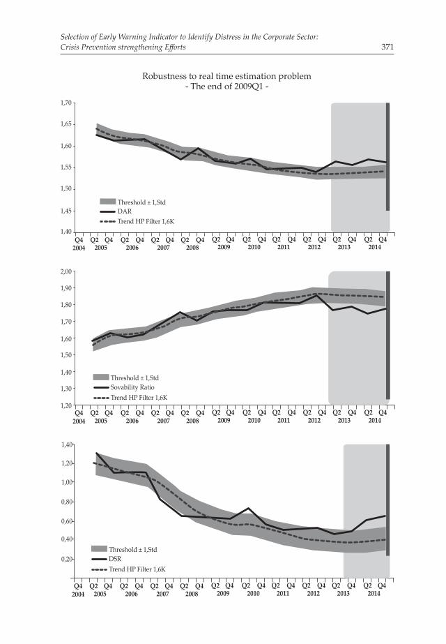
Selection of Early Warning Indicator to Identify Distress in the Corporate Sector: Crisis Prevention strengthening Efforts 371
Robustness to real time estimation problem- The end of 2009Q1 -
Current Ratio (CR)1,70
1,60
1,50
1,40
1,30
1,20
1,10
100
0,90
0,80
Threshold ± 1,StdCurrent Ratio Trend HP Filter 1,6K
Q42004
Q2 Q42005
Q2 Q42006
Q2 Q42007
Q2 Q42008
Q2 Q42009
Q2 Q42010
Q2 Q42011
Q2 Q42012
Q2 Q42013
Q2 Q42014
100
1,60
1,50
1,40
1,30
1,20
1,10
0,90
0,80
Threshold ± 1,StdCurrent RatioTrend HP Filter 1,6K
Q42004
Q2 Q42005
Q2 Q42006
Q2 Q42007
Q2 Q42008
Q2 Q42009
Q2 Q42010
Q2 Q42011
Q2 Q42012
Q2 Q42013
Q2 Q42014
Current Ratio (CR)
Threshold ± 1,StdQuick RatioTrend HP Filter 1,6K
0,90
0,80
0,70
0,60
0,50
0,40
0,30Q4
2004Q2 Q4
2005Q2 Q4
2006Q2 Q4
2007Q2 Q4
2008Q2 Q4
2009Q2 Q4
2010Q2 Q4
2011Q2 Q4
2012Q2 Q4
2013Q2 Q4
2014
0,80
0,75
0,70
0,65
0,60
0,55
0,50
0,45
0,40
0,35
0,30
Threshold ± 1,StdCurrent RatioTrend HP Filter 1,6K
Q42004
Q2 Q42005
Q2 Q42006
Q2 Q42007
Q2 Q42008
Q2 Q42009
Q2 Q42010
Q2 Q42011
Q2 Q42012
Q2 Q42013
Q2 Q42014
Debt Equity Ratio (DER)
Q42004
Q2 Q42005
Q2 Q42006
Q2 Q42007
Q2 Q42008
Q2 Q42009
Q2 Q42010
Q2 Q42011
Q2 Q42012
Q2 Q42013
Q2 Q42014
2,00
1,80
1,60
1,40
1,20
1,00
0,80
0,60
0,40
Threshold ± 1,StdDERTrend HP Filter 1,6K
2,00
1,80
1,60
1,40
1,20
1,00
0,80
0,60
0,40
0,20
-
Threshold ± 1,StdDERTrend HP Filter 1,6K
Q42004
Q2 Q42005
Q2 Q42006
Q2 Q42007
Q2 Q42008
Q2 Q42009
Q2 Q42010
Q2 Q42011
Q2 Q42012
Q2 Q42013
Q2 Q42014
Debt Asset Ratio (DAR)
1,70
0,65
0,60
0,55
0,50
0,45
0,40
Threshold ± 1,StdDARTrend HP Filter 1,6K
Q42004
Q2 Q42005
Q2 Q42006
Q2 Q42007
Q2 Q42008
Q2 Q42009
Q2 Q42010
Q2 Q42011
Q2 Q42012
Q2 Q42013
Q2 Q42014
1,70
1,60
1,65
1,50
1,55
1,40
1,45Threshold ± 1,StdDARTrend HP Filter 1,6K
Q42004
Q2 Q42005
Q2 Q42006
Q2 Q42007
Q2 Q42008
Q2 Q42009
Q2 Q42010
Q2 Q42011
Q2 Q42012
Q2 Q42013
Q2 Q42014
1,40
1,20
1,00
0,80
0,60
0,40
0,20
-Q4
2004Q2 Q4
2005Q2 Q4
2006Q2 Q4
2007Q2 Q4
2008Q2 Q4
2009Q2 Q4
2010Q2 Q4
2011Q2 Q4
2012Q2 Q4
2013Q2 Q4
2014
Threshold ± 1,StdDSRTrend HP Filter 1,6K
Debt Service Ratio (DSR)
1,40
1,20
1,00
0,80
0,60
0,40
0,20
-Q4
2004Q2 Q4
2005Q2 Q4
2006Q2 Q4
2007Q2 Q4
2008Q2 Q4
2009Q2 Q4
2010Q2 Q4
2011Q2 Q4
2012Q2 Q4
2013Q2 Q4
2014
Threshold ± 1,StdDSRTrend HP Filter 1,6K
2,00
1,90
1,80
1,70
1,60
1,50
1,40
1,30
1,20Q4
2004Q2 Q4
2005Q2 Q4
2006Q2 Q4
2007Q2 Q4
2008Q2 Q4
2009Q2 Q4
2010Q2 Q4
2011Q2 Q4
2012Q2 Q4
2013Q2 Q4
2014
Threshold ± 1,StdSovability Ratio Trend HP Filter 1,6K
Solvability Ratio (SR)2,20
2,00
1,80
1,60
1,40
1,20
1,00Q4
2004Q2 Q4
2005Q2 Q4
2006Q2 Q4
2007Q2 Q4
2008Q2 Q4
2009Q2 Q4
2010Q2 Q4
2011Q2 Q4
2012Q2 Q4
2013Q2 Q4
2014
Threshold ± 1,StdSovabilitiy RatioTrend HP Filter 1,6K
1,40
1,20
1,00
0,80
0,60
0,40
0,20
-Q4
2004Q2 Q4
2005Q2 Q4
2006Q2 Q4
2007Q2 Q4
2008Q2 Q4
2009Q2 Q4
2010Q2 Q4
2011Q2 Q4
2012Q2 Q4
2013Q2 Q4
2014
Threshold ± 1,StdDSRTrend HP Filter 1,6K
Debt Service Ratio (DSR)
1,40
1,20
1,00
0,80
0,60
0,40
0,20
-Q4
2004Q2 Q4
2005Q2 Q4
2006Q2 Q4
2007Q2 Q4
2008Q2 Q4
2009Q2 Q4
2010Q2 Q4
2011Q2 Q4
2012Q2 Q4
2013Q2 Q4
2014
Threshold ± 1,StdDSRTrend HP Filter 1,6K
2,00
1,90
1,80
1,70
1,60
1,50
1,40
1,30
1,20Q4
2004Q2 Q4
2005Q2 Q4
2006Q2 Q4
2007Q2 Q4
2008Q2 Q4
2009Q2 Q4
2010Q2 Q4
2011Q2 Q4
2012Q2 Q4
2013Q2 Q4
2014
Threshold ± 1,StdSovability Ratio Trend HP Filter 1,6K
Solvability Ratio (SR)2,20
2,00
1,80
1,60
1,40
1,20
1,00Q4
2004Q2 Q4
2005Q2 Q4
2006Q2 Q4
2007Q2 Q4
2008Q2 Q4
2009Q2 Q4
2010Q2 Q4
2011Q2 Q4
2012Q2 Q4
2013Q2 Q4
2014
Threshold ± 1,StdSovabilitiy RatioTrend HP Filter 1,6K

Bulletin of Monetary Economics and Banking, Volume 20, Number 3, January 2018372
Overall, robustness test results indicated that the indicator is robust enough to provide signals before the distress event period. Based on Table 4, the loss generated by the out of sample tends to be smaller when compared to the analysis of all samples with the same prediction accuracy.
Table 4. Statistical Evaluation Result Comparison:All Samples vs Real Time Estimation Problem
Indikators
AGGREGATE
Kategori Model Trend
CR
QR
DER
DAR
SR
DSR
Liquidity Indicator
Liquidty Indicator
Solvency Indicator
Solvency Indicator
Solvency Indicator
Solvency Indicator
one-sided HP Filter
one-sided HP Filter
one-sided HP Filter
one-sided HP Filter
one-sided HP Filter
one-sided HP Filter
0,131
0,083
0,095
0,107
0,131
0,95
2008Q2
200Q2
2007Q4
2008Q2
2008Q2
2008Q1
80%
80%
80%
80%
80%
80%
0,111
0,056
0,028
0,28
0,28
0,083
80%
80%
80%
80%
80%
80%
Threshold PredictivePower Loss First Signal
(Distress : 2009Q1Predictive
Power
Robuness to real timeestimation problem- The end of 2009Q1
Assessment for all period
Loss
= 0,5µ
= 0,5µ
= 0,5µ
= 0,5µ
= 0,5µ
= 0,5µ
𝜆𝜆= 1600
1𝛔𝛔 (Lower)
1𝛔𝛔 (Lower)
1𝛔𝛔 (Upper)
1𝛔𝛔 (Upper)
1𝛔𝛔 (Lower)
1𝛔𝛔 (Upper)
Leading Indicator Near-Term Indicator
V. CONLUSIONS5.1. ConclusionsBased on the results of the analysis it can be summarized that:1. The result of Noise to Signal Ratio (NSR) analysis revealed that the long-term
trend obtained through the one-sided HP filter method was better in giving distress signal when compared to Moving Average.
2. The statistical evaluation of several potential EWI for corporate financial distress showed that some indicators can signal early distress or vulnerability in the non-financial corporate sector in terms of aggregate such as Debt to Equity Ratio (DER) as a leading indicator and Current Ratio (CR)), Quick Ratio (QR), Debt to Asset Ratio (DAR), Solvability Ratio (SR), and Debt Service Ratio (DSR) as near-term indicator.
3. For sectoral, there are 4 leading indicators, namely (a) DER for agriculture, miscellaneous industry and property & real estate sector; (b) DSR for basic & chemical industry sectors; (c) DAR for various industrial sectors; and (d) Asset Turnover for trade, services and investment sectors.
4. In addition, there are some sectors that have near term indicator, including (a) the agriculture sector (Capital Expenditure to Depreciation & Amortization); (b) infrastructure, utilities and transportation sectors (Interest Coverage Ratio, Inventory Turnover and Asset Turnover); (c) various industries (Solvability Ratio (SR); (d) mining sector (Return on Assets, ROA; and Return on Equity, ROE); and (e) trade, services and investment sectors (Quick Ratio, QR).

Selection of Early Warning Indicator to Identify Distress in the Corporate Sector: Crisis Prevention strengthening Efforts 373
5. The identified Early Warning Indicator (EWI), both sectorally and aggregately, can be used to identify the occurrence of corporate sector distress. Thus, efforts to prevent rising risks that could lead to a financial crisis can be anticipated earlier and the stability of the financial system will be maintained.
6. Given the fact that the identification of EWI signaling capability is based on historical data behavior, it can not catch changes in the behavior of economic actors in the future. Thus, the use of this EWI still needs to be complemented by other indicators.
5.2. Future Development AreasTo improve the analysis results, there are several future development agenda such as:1. It is necessary to examine the use of other methodologies related to the
preparation of EWI such as the Area Under Receiver Operating Characteristic (AUROC) curves to improve the analysis results obtained in this research.
2. This methodology can then be applied to other sectors of the economy so that a comprehensive financial activity indicator and heatmap can be obtained.
REFERENCESAllen et al. (2002). A Balance Sheet Approach to Financial Crisis. IMF Working Paper,
WP/02/210.Altman, E. I. dan Hotchkiss, E. (2006). Corporate Financial Distress and Bankcrupty
3rd Edition. New York: John Wiley and Son, Inc.Andrade, G. dan Kaplan, S. N. (1998). How Costly Is Financial (Not Economic)
Distress? Evidence from Highly Leveraged Transactions That Became Distressed. The Journal of Finance, Vol. 53, No. 5. (Oct., 1998), pp. 1443-1493.
Asquith P., Gertner, R. dan Scharfstein, D. (1994). Anatomy of Financial Distress: An Examination of Junk-Bond Issuers. Quarterly Journal of Economics, 109: 1189-1222.
Bhunia, A., Uddin Khan, S. I. dan Mukhuti, S. (2011). Prediction of Financial Distress - A Case Study of Indian Companies. Asian Journal of Business Management,3(3), 210-218.
Blancher, N., et. al. (2013). Systemic Risk Monitoring (―SysMo‖) Toolkit—A User Guide. IMF Working Paper, WP/13/168.
Drehmann, M., et. al. (2010). Countercyclical capital buffers: exploring options. ((BIS) Working Papers No. 317).
Drehmann, M., Borio, C. dan Tsatsaronis, K. (2011). Anchoring countercyclical capital buffers: the role of credit aggregates. ((BIS) Working Papers No. 355).
Fitzpatrick. (2004). An Empirical Investigation of Dynamics of Financial Distress. A Dissertation Doctor of Philosophy, Faculty of the Graduate School of the State University of New York at Buffalo, USA.
Gapen, M. T., et. al. (2004). The Contingent Claims Approach to Corporate Vulnerability Analysis: Estimating Default Risk and Economy-Wide Risk Transfer.IMF Working Paper, WP/04/121.
Gray, D dan Malone, S.W. (2009). Macrofinancial Risk Analysis. England: John Wiley

Bulletin of Monetary Economics and Banking, Volume 20, Number 3, January 2018374
& Sons, Inc. Ishikawa, A., et. al. (2012). The Financial Activity Index. (Bank of Japan Working
Paper Series, No.12-E-4).Ito, Y., et. al. (2014). New Financial Activity Indexes: Early Warning System for Financial
Imbalances in Japan. (Bank of Japan Working Paper Series, No.14-E-7).Jakubík, P. dan Teplý, P., (2011). The JT Index as an Indicator of Financial Stabilityof Corporate Sector. Prague Economic Papers, 2011(2), 157-176.Bank Indonesia. (2009). Kajian Stabilitas Keuangan. Jakarta: Bank Indonesia.Luciana Spica Almilia. (2004). Analisis Faktor-faktor yang Mempengaruhi Kondisi
Financial Distress suatu Perusahaan yang Terdaftar di Bursa Efek Jakarta. Jurnal Riset Akuntansi Indonesia, Vol. 7. No. 1: 1-22.
Platt, H., dan Platt, M. B. (2002). Predicting Financial Distress. Journal of Financial Service Professionals, 56: 12-15.
Pranowo, K., et. al. (2010). Determinant of Corporate Financial Distress in an Emerging Market Economy: Empirical Evidence from the Indonesian Stock Exchange 2004-2008. International Research Journal of Finance and Economics, Issue 52.
Surjaningsih, N., Yumanita, D. dan Deriantino, D. (2014). Early Warning Indicator Risiko Likuiditas Perbankan. Bank Indonesia Working Paper No. 1.
Wiehle, U., et. al. (2005). 100 IFRS Financial Ratios.Wiesbaden, Germany: Cometis AG.
AppendixNetwork Analysis Result Based on Financial Account Data & Balance Sheet
Gross Exposure 2015Q2 Net Exposure 2015Q2
ODC - HH4.486,09
ROW -NFC5.886,31
NFC - ODC3.286,84
ODC11.482,57
HH7.732,69
OFC4.468,37
LG928,17
CG4.412,87
NFC
14.542,04
ROW
11.675,38
CB3.356,06
Gross Exposure 2015Q2
Source: Bank Indonesia
-151,39
-12,79
-3,71
27,56
HH-> NFC47,19
5,23
5,91
58,12
71,04ROW
CG
CB
HH
OFC
LG
ODCNFC
Net Exposure 2015Q2
Net Inflow
Net Outflow

NOWCASTING HOUSEHOLD CONSUMPTION AND INVESTMENT IN INDONESIA
Tarsidin, Idham, Robbi Nur Rakhman1
1. The authors would like to express appreciation to Yoga Affandi and Sahminan for their input, Ferry Kurniawan for his assistance and Prof. Dr. Abuzar Asra and authors’ colleagues at the Economic and Monetary Policy Department (DKEM) for their input. The email addresses of the authors are as follows: [email protected], [email protected], and [email protected]. The opinions expressed in this paper are those of the authors and do not necessarily represent the position or policy of Bank Indonesia.
It is imperative for the Central Bank to know the current state of the economy as the basis underlying projections of future economic conditions. To that end, current economic conditions, in this case household consumption and investment, could be predicted using nowcasting. In this research, a nowcasting model was developed for the two aforementioned macroeconomic variables using a Dynamic Factor Model (DFM). The indicators used when nowcasting household consumption included: motor vehicle sales, total deposits, the lending rate on consumer loans, M1, and the Rupiah Exchange Rate (NEER), while the indicators used for nowcasting investment included: cement sales, motor vehicle production, electric energy consumption, outstanding loans, and M1. Accuracy testing showed that the nowcasting model for household consumption using DFM was sound, while the forecast error for nowcasting investment was significant but remained below the benchmark.
Keywords: Nowcasting, Mixed Frequency Regression, Dynamic Factor ModelJEL Classification: C38, C53
ABSTRACT

Bulletin of Monetary Economics and Banking, Volume 20, Number 3, January 2018376
I. INTRODUCTIONAccording to the Forecasting and Policy Analysis (FPAS) framework, Bank Indonesia utilises the ARIMBI core model and several satellite models, such as SOFIE, MODBI, ISMA, and BIMA. The five models are fundamentally macroeconomic models used for short-term (up to two years) and medium-term (2-5 years) projections. In addition, Bank Indonesia also has several indicator models, including GDP, inflation and exchange rate models, which are used to produce near-term forecasts (for the current quarter and subsequent period) as well as nowcasting (current quarter).
Indicator models are crucial considering the importance of the Central Bank knowing the current state of the economy as the basis underlying projections of future economic conditions in line with international best practices at other central banks, including the Riksbanken and Bank of England.2 Furthermore, projections based on the indicator models are used as inputs for the macroeconomic models. Therefore, projections for the current quarter and subsequent period are fundamentally generated by the indicator models.
Considering the importance of indicator models, further development was required. Currently, Bank Indonesia only has indicator models for GDP, inflation, and the exchange rate but is lacking models for GDP components, such as consumption, investment, and exports/imports. This research developed an indicator model for nowcasting household consumption and investment. The model was expected to improve the accuracy of Bank Indonesia’s economic projections and, therefore, support more precise monetary policymaking.
Nowcasting has developed rapidly over the past decade. The most commonly used methods include Bridge Equation, Mixed Data Sampling (MIDAS) developed by Ghysels, et al. (2004)), Mixed Frequency VAR (MF-VAR developed by Mariano and Murasawa (2010) as well as Schorfheide and Song (2013)) and the Dynamic Factor Model (DFM, otherwise known as the Mixed Frequency Factor Model (MF-FM), developed by Mariano and Murasawa (2003) and Giannone, et al. (2008)).
Nowcasting GDP in Indonesia has been performed by Kurniawan (2014) using the MIDAS approach along with the Mixed Frequency Factor Model, as well as by Luciani, et al. (2015) using the Dynamic Factor Model. Nowcasting has been proven to effectively bolster economic assessments in Indonesia.
II. THEORYUnder the ITF framework, it is imperative that Bank Indonesia is constantly aware of the current state of the economy and how close the economy is to equilibrium as the basis underlying projections of future economic conditions. By knowing the state of the economy and projections of upcoming conditions, Bank Indonesia can determine the appropriate monetary policy response to adopt. Over the past decade, nowcasting has been developed to assess the current state of the economy.
2. As cited by Angelini, et al. (2008), Andersson and Reijer (2015) as well as Bell, et al. (2014) amongst others.

Nowcasting Household Consumption and Investment in Indonesia 377
The term nowcasting defines the projections of a macroeconomic variable, for instance GDP, for the current quarter using higher frequency data.
2.1. Nowcasting for Economic AssessmentPrior to the 1990s, economic assessments were primarily based on the economic index developed by Burns and Mitchell (1946). The (US) Conference Board and OECD further developed the economic index, which was fundamentally an estimation of the business cycle by extracting the cycles of various series,3 determining the turning points4, determining the indicators with similar dynamics as the reference series and regressing into a single index. The Coincident Economic Index developed by the Conference Board and OECD illustrated the current state of the economy using nonfarm payrolls, personal income (after transfers), the industrial production index, as well as manufacturing and trade sector sales.
Nonetheless, various innovative new approaches began to appear around 1990 to estimate the coincident economic index using econometric methods. One such approach was developed by Stock-Wilson (1989) using Maximum Likelihood Factor Analysis, which is considered a milestone in the development of nowcasting.
Nowcasting, which is a method to project the state of the economy, was developed around the start of the 21st century. There are similarities between the coincident economic index and nowcasting, namely that both using high-frequency indicators to capture the dynamics of a reference series (for example GDP). The difference is that the coincident economic index is a composite of various indicators with similar dynamics as the reference series, while nowcasting is an estimation of the magnitude of the reference series using representative indicators. Unlike the coincident economic index, nowcasting not only estimates the direction of current economic conditions but also the magnitude. Seminal papers on nowcasting include Bridge Equation Mariano and Murasawa (2203), Ghysels, et al. (2004), Giannone, et al. (2008) and Doz, et al. (2011).
Bańbura, et al. (2012) suggested that ideally, a nowcasting model would formulate several major characteristics relating to market behaviours and institute policy referring to actual data in real-time. In relation to the nowcasting model, Bell, et al. (2014), applied two methods, namely the industry model and the weighted survey model. The industry model used industry-level data and a series of indicators for nowcasting GDP, while the weighted survey model merely relied on survey indicators (excluding formally published data).
There is now a range of literature that deals with nowcasting GDP for economic assessment. Nowcasting in the UK was conducted by Bell, et al. (2014), in the Euro area by Angelini, et al. (2008) and in Sweden by Andersson and Reijer (2015). Furthermore, nowcasting has also been performed in Indonesia by Kurniawan (2014) and Luciani, et al. (2015).
3. Using the Phase Average Trend (PAT) method, Hodrick-Prescott (HP) filter or Christiano-Fidgerald (CF) filter as per the OECD (2012).4. Using the Bry-Boschan algorithm.

Bulletin of Monetary Economics and Banking, Volume 20, Number 3, January 2018378
In addition to nowcasting GDP, nowcasting other variables (such as inflation) as well as components of GDP (including household consumption and investment) has also been achieved but the literature remains limited. Nowcasting of GDP components was performed by Baffigi, et al. (2004), amongst others, who conducted nowcasting using the Bridge Equation Method. The results showed that the retail sales index is an important component of household consumption, while the Consumer Confidence Index (CCI) plays only a minor role (possibly due to correlation with other indicators). Motor vehicle registrations was another indicator with close correlation to the consumption of durable goods. On the other hand, however, survey data was found to represent a sound proxy of investment, particularly the short-term dynamics of demand along with construction.
Sørensen (2011) stated that considering the large contribution of household consumption to GDP, household consumption is an important factor when assessing the state of the economy. A simple regression (OLS) nowcasting method was used à la Bridge equation, where the indicator was selected using the general-to-specific approach based on information criteria, model reduction tests and misspecification tests. The salient indicators found by Sørensen (2011) included: new registrations of passenger vehicles, the velocity of money and the Consumer Confidence Index (CCI), while the retail sales index was not found to be significant.
2.2. Nowcasting MethodAs mentioned previously, several nowcasting methods are commonly used, including Bridge Equation, Mixed Data Sampling (MIDAS), Mixed Frequency VAR, and Mixed Frequency Factor Model (often referred to as Dynamic Factor Model). The four methods are explored in the following section, as cited in Foroni and Marcellino (2013).
1) Bridge EquationThe Bridge Equation is a linear regression that correlates high-frequency variables (for instance monthly retail sales) with lower frequency variables (quarterly GDP for example), thereby producing an estimation of the latest economic conditions prior to the release of the quarterly data. This method was introduced by Baffigi, et al. (2004). The Bridge model can be expressed as the following equation:
(2.1)
where: yt : reference series (quarterly)xt : monthly indicators aggregated to quarterly indicatorsβi (L) : lag polynomial coefficients
The Bridge Equation is resolved through two stages as follows: (i) the monthly indicators are projected for the current quarter (for instance using ARIMA or VAR)

Nowcasting Household Consumption and Investment in Indonesia 379
and then aggregated to obtain a quarterly value; and (ii) the aggregated indicator value is set as the regressor. Bańbura, et al, (2012) found that the Bridge Equation only captured limited aspects of the nowcasting process, which is understandable considering the monthly indicators are aggregated into quarterly data, thus some of the latest information is lost.
2) Mixed Data SamplingThe aggregation process involved in the Bridge Equation, where monthly indicators are aggregated into quarterly data, has the potential to lose some of the important information from the data. To overcome that problem, an estimation method was developed based on mixed frequency data. Ghysels, et al. (2004) introduced a method known as Mixed Data Sampling (MIDAS). In this case, the dependent variable yt (representing lower-frequency, quarterly data) is regressed against a distributed lag of xt (representing higher-frequency, monthly data). The MIDAS equation can be specified as follows:
(2.2)
where: yt : reference series (quarterly)xt : monthly indicators b(L1⁄m;θ)=∑K
k=0c(k;θ) Lmk : lag polynomial coefficients
The main characteristic of MIDAS is that the parameterisation of the lagged coefficients c(k;θ) is modelled using the parsimonious distributed lag polynomials in order to avoid parameter proliferation that could emerge as well as issues related to the selection of the lag-order. In this case, parameterisation can be achieved using the exponential Almon lag, Beta lag, linear scheme, hyperbolic scheme, and geometric scheme.
Bańbura, et al. (2012) suggested that MIDAS represents an improvement on the Bridge Equation, which is understandable because MIDAS is fundamentally similar to the Bridge Equation. The only difference is that the temporal aggregation of mixed-frequency indicators is omitted. Nonetheless, MIDAS contains the problem of dimensionality and is limited in terms of the number of variables. A further review of MIDAS was conducted by Andreou, et al. (2010), who decomposed the MIDAS regression into two components, namely an aggregate component with the same weighting and a nonlinear component, and compared them to the Conventional Least Square Regression (temporal aggregation with the same weighting). The results showed that the MIDAS estimator is more efficient (robust).
3) Mixed Frequency VARAnother common nowcasting approach is the Mixed Frequency VAR, for instance using a quarterly reference series and a monthly component series (indicators). By modelling the reference series and component series simultaneously, co-

Bulletin of Monetary Economics and Banking, Volume 20, Number 3, January 2018380
movement between the reference series and mixed frequency indicators can be analysed. Two Mixed Frequency VAR (MF-VAR) approaches are presented in the literature, namely the classical approach developed by Mariano and Murasawa (2010) as well as the Bayesian approach developed by Schorfheide and Song (2013). The MF-VAR equation can be express as follows:
where: y*tm : reference series (latent m-to-m growth)xtm
: monthly indicators Lm : lag operator
4) Mixed Frequency Dynamic Factor ModelThe Mixed Frequency Dynamic Factor Model is another common nowcasting approach. Using a factor model, the unobserved state of the economy is extracted and a new coincident indicator is constructed. More information is obtained using this approach and the projections estimated are more accurate. The methodology was developed from the Stock-Watson coincident index by Mariano and Murasawa (2003) for small-scale models and by Giannone, et al. (2008) for large-scale models. A detailed description of the methodology is presented in Bańbura, et al. (2011a).
Giannone, et al. (2008), as cited by Angelina, et al. (2008) and Foroni and Marcellino (2013), coined the approach, bridging with factors, considering the (quarterly) reference series is regressed with the (monthly) common factors as a form of bridging equation. As a preliminary step, the common factors are extracted from the monthly data series on a large scale using a two-step estimator. The model specification can be expressed as follows:
(2.3)
(2.4)
(2.5)
5. For explanations on state space models and the Kalman filter refer to Hamilton (1994).
where: xtm
: monthly indicatorsftm
: common factorsΛ : factor loadings ξtm
: idiosyncratic component
The monthly common factors are subsequently averaged. Time aggregation is applied by aligning the quarterly data with that of the third month in the respective quarter, while the first and second months data are calculated using the Kalman filter.5 The next stage involves projecting the reference series, for instance

Nowcasting Household Consumption and Investment in Indonesia 381
the quarterly GDP series, based on the estimated common factors that have been regressed into quarterly data. The equation can be expressed as follows:
(2.6)
where: : quarterly reference series : quarterly aggregated
Doz, et al. (2011) demonstrated consistency between the two-step estimator and maximum likelihood. In this case, the asymptotic properties were tested with various misspecifications. The results showed that the Factor Model with a maximum likelihood was robust to the misspecifications. Furthermore, Doz, et al. (2011) proposed two-step procedures to estimate the common factors when the model parameters are unknown. The first step is to calculate the preliminary estimators of the factors and estimators of the model parameters using Principal Component Analysis (PCA). The second stage involves calculating the heteroscedasticity of the idiosyncratic components and/or common factor dynamics. The actual values of the parameters are subsequently replaced with the estimations according to PCA and the factor dynamics are estimated from the preliminary estimates of the respective factors.
Bańbura and Rünstler (2011) developed the Factor Model by combining the model with the projection equation for quarterly GDP growth using the mixed-frequency approach similar to Mariano and Murasawa (2003) in order to include a static equation that linked the common factors (ft) with the latent variables in the form of monthly GDP growth (yt), which can be expressed as follows:
where: yt : reference seriesft : common factorsεt : white noise error
The Dynamic Factor Model was subsequently developed further by Aruoba, et al. (2012) in order to use mixed-frequency and high-frequency data (including weekly, monthly and continuous data). As confirmed by Aruoba, et al. (2012), Stock and Wilson (1989) did not model the Factor Model with mixed-frequency and high-frequency data, while Mariano and Murasawa (2003) only modelled mixed-frequency data not high-frequency data.
Bańbura and Rünstler (2011) also developed the model by deriving the weighting of each indicator in the model, thereby revealing the actual contribution of each respective indicator to the projection. Meanwhile, Diebold and Rudebusch (1996) stressed the need for a regime switching synthesis in the Dynamic Factor Model and explored a framework to that end. In addition, the interplay between the reference series and its common factors should be observed, as modelled using
(2.7)

Bulletin of Monetary Economics and Banking, Volume 20, Number 3, January 2018382
6. Refer to Andersson and Reijer (2015).7. Refer to Angelina, et al. (2008).8. Refer to Kurniawan (2014).9. Refer to Luciani, et al. (2015).
(3.1)
(3.2)
Factor-Augmented Vector Autoregression (FAVAR) mentioned by Andersson and Reijer (2015).
III. METHODOLOGY3.1. MethodNowcasting using the Factor Model is commonly used by central banks to predict current quarter GDP, including the Riksbanken6, Norges Bank, European Central Bank (ECB)7, Bank Indonesia8, and by international organisations including ADB9. The capacity to accommodate numerous indicators ensures the popularity of the Factor Model. Nowcasting household consumption and investment is not dissimilar to nowcasting GDP. Therefore, the nowcasting method typically used for GDP can also be applied to nowcasting other lower-frequency variables (including household consumption and investment), as suggested by Bańbura, et al (2011b).
The preferred method in this research is the Mixed Frequency Dynamic Factor Model (abbreviated to DFM). There are a number of significant variations to the estimates and projections using DFM. In this research, the authors were inclined to follow the approach of Giannone, et al. (2008), developed by Bańbura and Rünstler (2011) and modified by Kurniawan (2014). The model specification can be expressed as follows:
where: zt : consists of reference series (yt) and monthly indicators (xt)ft : common factorsΛ : factor loadings ut : idiosyncratic component βt : consists of common factors (ft) and idiosyncratic component (ut)F : autoregressive coefficientsεt : white noise error
The state space in Equations 3.1 and 3.2 was built in the form of a matrix as follows:

Nowcasting Household Consumption and Investment in Indonesia 383
Measurement Equation:
Transition Equation:

Bulletin of Monetary Economics and Banking, Volume 20, Number 3, January 2018384
Equations 3.1 and 3.2 were estimated in two stages, known as the two-step estimator. The first stage involved estimating the representative parameters of the state space using the principal components (from the balanced panel of monthly indicators10), thus estimating the magnitude of the common factors. In the second stage, the common factors were re-estimated by applying a Kalman smoother to the entire information set. The reference series (household consumption and investment) was subsequently projected by regressing the latent variables in the form of year-on-year household consumption growth and year-on-year investment growth against the common factors.
3.2. DataThe data used in this research was for the period from 2003-2015. The estimations were based on data from 2003-2015 and the pseudo out-of-sample testing used 2015 data. The reference series were household consumption and investment, while the component series were various representative indicators selected from a range of candidate indicators. The reference series had a quarterly frequency and the data is published by BPS-Statistics Indonesia. Meanwhile, the indicators in the component series were mixed frequency, with the majority in the form of monthly data. Not all data for the indicators was available from 2003-2015. Therefore, the data was ragged data with differing availability across the period.
Since 2015, BPS-Statistics Indonesia has released data using 2010 as the base year for 2010-2015 data. Previous BPS data used 2000 as the base year. In a departure from the previous data, household consumption data using 2010 as the base year does not contain the consumption of non-profit institutions. Data with a base year of 2010 was applied in this research, therefore the data did not contain the consumption of non-profit institutions. For earlier years (2003-2009), however, backcasting was applied to the growth in order to obtain household consumption without the consumption of non-profit institutions. Similarly, for investment the data used had a base year of 2010, so for previous years backcasting was again applied.
The data was divisible into soft data and hard data, as suggested by Bańbura and Rünstler (2011) as well as Bańbura, et al. (2012). Soft data (such as survey data and financial data) is available before hard data (such as statistical data released by BPS-Statistics Indonesia). Hard data contains more reliable information. The representative indicators were also categorised as hard indicators and soft indicators, consistent with Angelina, et al. (2008). Hard indicators are released later than soft indicators but the data contained is more reliable. The contribution of soft data is large at the beginning of the quarter but small at the end and vice versa for hard data. Considering the different contributions, the two types of data were also assigned different weights. Bańbura and Rünstler (2011) stated that hard data (real activity data) is an invaluable source of information but when the late
10. As mentioned by Bańbura, et al. (2012), xt only contains observable monthly indicators, thus omitting quarterly series of household consumption and investment, as well as monthly latent series.

Nowcasting Household Consumption and Investment in Indonesia 385
publication is taken into account, hard data becomes less relevant. In this case, survey and financial data become more important.
3.3. StagesThe stages of nowcasting household consumption and investment involved:
indicator selection, filtering and transformation, the nowcasting exercise, and model performance evaluation.
1) Indicator Selection Although the modelling was not required to find causality between the
component series and reference series, this does not imply that any indicator could be inputted to the model. The indicators should have a close relationship with their reference series, in this case household consumption and investment (PMTB). OECD (2012) found that their economic relevance must be considered when selecting the indicators (economically significant and a broad scope). In a different context (leading indicators, not coincident indicators), OECD (2012) stated that the indicators should meet one of the following criteria: early stage, rapidly responsive, expectation-sensitive or prime mover. Similar findings were put forward by Riksbanken, cited by Andersson and Reijer (2015), namely that the selected indicators should influence the business cycle, the variables should react at the beginning of the business cycle and the series should gauge the beginning of the production chain as well as the expectations of economic agents (typically collated from surveys).
In addition to economic relevance, a number of other requirements must also be met. OECD (2012) stressed the need for an indicator with a monthly frequency that is rarely revised, published on time and with a long data series. During the initial stage, several candidate indicators were selected that meet the requirements in terms of economic relevance and practical considerations. The candidate indicators were subsequently whittled down using several criteria in order to observe the correlation with the reference series (based on the coefficient of correlation) and similarity of the common factors with the reference series (based on Principal Component Analysis). Several indicators were thus selected for use in the estimations. In the literature, relatively large data sets were also used, exceeding 50 variables, arguing that each variable contains specific information about the economy that might be absent from the other variables.
2) Filtering and Transformation Prior to use in the estimations, the data must be filtered using seasonal
adjustments with X-12 or TRAMO/SEATS. More robust estimations are possible by omitting seasonal factors from the reference series and component series. Nonetheless, when the data was used for projections, the prediction was the actual value that contains seasonal factors. Therefore, the results must be multiplied or added to the seasonal factors for comparison with the realised data.

Bulletin of Monetary Economics and Banking, Volume 20, Number 3, January 2018386
Another common approach is to exclude the seasonal adjustment. Therefore, direct comparisons with the realised data are possible. This approach is appropriate if similar seasonal factors are found in the reference series and component series. The estimations may be compromised, however, if the seasonal factors are different in the reference series and component series, leading to less robust estimations. Considering that the data on household consumption and investment released by BPS-Statistics Indonesia has not had the seasonal factors removed, seasonal adjustments were preferred in this research.
The correlation between the reference series and component series (indicators) depends on whether the indicators are stock data or flow data, and how the indicators are transformed before being inputted into the model (for instance the stationarity requirements), as suggested by Bańbura, et al. (2012). Data may be presented in the form of level, percentage, index or unit. Level data was based on constant prices (real value). Data in level, index and unit were transformed into year-on-year growth. Percentage data, on the other hand, was transformed into the difference with the previous year. The reference series and indicators were then standardised for comparison.
3) Nowcasting Exercise As mentioned previously, the estimations were made using the Dynamic
Factor Model and data for the period from 2003-2015. In this case, a nowcasting exercise was conducted systematically using various combinations of component series, namely consisting of 4, 5, and 6 indicators from the range of candidate indicators selected. The best model was chosen based on pseudo out-of-sample testing of the data from 2015 to predict household consumption and investment in each quarter of the year. The model with the smallest RMSE was selected, demonstrating that the prediction model was more accurate.
A more rigorous test was conducted for the fourth quarter of 2015, namely weekly predictions for the first, second, and third months in line with data availability (released data). To that end, the approach of Camacho and Perez-Quiros (2010) was used to evaluate the results of the nowcasting exercise by using real-time conditions and revised data. Consequently, a real-time dataset was built consisting of vintage data (historical data) available for each of the nowcasting data points.
To enhance the prediction capabilities, Giannone, et al. (2008) as well as Bańbura and Rünstler (2011) proposed uncertainty measures (that show the marginal gain on the prediction precision) to assess the role of latest data releases. Furthermore, Bańbura and Rünstler (2011) stressed the need for different weightings on each indicator in every prediction period. Therefore, when using the prediction model, different indicators could be used or even large datasets (consisting of timely indicators and/or indicators containing important information).

Nowcasting Household Consumption and Investment in Indonesia 387
4) Model Performance Evaluation The next stage involves evaluating the performance of the selected model.
The evaluation takes into account a comparison with the benchmark models, including the Bridge Equation and ARIMA model. A comparison with the Bridge Equation was chosen due to the simplicity of the model. Meanwhile, the ARIMA model is known for its near-term forecasting accuracy compared to naïve methods and other simple models.
IV. RESULTS AND ANALYSISThe following section explores the results of the indicator selection, data management as well as estimations and predictions using the Dynamic Factor Model (DFM). In this case, a number of models with several different combinations of indicators were estimated in order to produce a more robust nowcasting model.
4.1. Indicator SelectionAs mentioned previously, there were two requirements of indicator selection, namely economic relevance and practical considerations. Based on those considerations, a number of candidate indicators were selected for household consumption and investment that met both requirements, at least to some extent. From there, a number of candidate indicators were subsequently selected in order to observe their coefficient of correlation and contribution to explain the reference series for potential use in the estimations.
1) Indicators of Household Consumption Household consumption is the largest component of GDP. During the
observation period from 2003-2015, household consumption accounted for 54-63% of GDP. A number of indicators were found to have a high coefficient of correlation to household consumption as follows: • Indicators representing the magnitude of household consumption,
including motor vehicle sales and the retail sales index;• Indicators reflecting consumer opinion of economic conditions that
underlie their consumption decisions, including the consumer confidence index (composite, current economic condition, and expectation) as well as consumer tendency index;
• Economic performance indicators, which ultimately impact the level of household income and consumption, including the industrial production index, export YTD, import YTD, loading/unloading of cargo (through domestic and international ports), and the stock price index at the Indonesia Stock Exchange; and
• Indicators related to banking, economic liquidity, and exchange rates, which influence consumers’ consumption decisions, including total deposit, credit (consumer and total), 1, 3 and 6-month term deposit rates, the consumer lending rate, M1, M2 as well as the Rupiah exchange rate against the US dollar and the effective exchange rate, both nominal and real.

Bulletin of Monetary Economics and Banking, Volume 20, Number 3, January 2018388
Of the various candidate indicators mentioned, several indicators with the highest coefficient of correlation were selected. Table 1 presents the coefficients of correlation of several candidate indicators in terms of level and year-on-year growth (its difference for data in percentages) against household consumption. Indicators with a correlation coefficient value of 0.70 or more and a year-on-year growth correlation coefficient value of 0.15 or more as well as the correct correlation sign were selected for the evaluation stage.
Table 1.Correlation Coefficients of Indicators of Household Consumption
No. Indicators
Correlation Coefficient
LevelGrowth y-o-y(Its difference for data in %)
1 Motor vehicle sales 0.90 0.252 Retail sales index 0.97 0.303 Consumer confidence index:
CCI - composite 0.83 0.13CCI - current economic condition 0.89 0.19CCI - expectation 0.69 0.09
4 Consumer tendency index -0.24 0.005 Industrial production index 0.96 0.186 Export YTD 0.59 -0.157 Import YTD 0.36 -0.118 Loading/unloading of cargo:
Cargo loading in domestic ports 0.74 -0.34Cargo unloading in domestic ports -0.28 -0.17Cargo loading in international ports -0.30 -0.27Cargo unloading in international ports 0.78 -0.06
9 Stock price index at IDX 0.97 0.1910 Total deposit 0.98 0.4811 Credit:
Consumption 0.99 0.06Total 0.99 0.37
12 Deposit rate:1 month -0.59 -0.323 months -0.60 -0.326 months -0.63 -0.35
13 Consumer lending rate -0.92 -0.3414 M1 0.98 0.4115 M2 0.98 0.5416 Rupiah exchange rate:
Rupiah to USD 0.65 0.09NEER -0.91 -0.19REER 0.60 -0.39

Nowcasting Household Consumption and Investment in Indonesia 389
Based on those criteria, the following indicators were selected: motor vehicle sales, retail sales index, consumer confidence index - current economic condition, industrial production index, stock price index at the Indonesia Stock Exchange, total deposit, credit, consumer lending rate, M1, M2, and Nominal Effective Exchange Rate (NEER). To reduce the potential number of indicator combinations, a number of indicators were discarded due to their close resemblance to other indicators (with a higher correlation coefficient).
A number of practical considerations are presented in Table 2. All indicators have a monthly frequency, no (significant) data revisions and a publication lag of 7 days to 3 months. Despite a publication lag of 2-3 months, the industrial production index was included due to the important information contained in the indicator. A lag of three months was rare, with two months the norm.
Table 2.Practical Considerations of Indicators of Household Consumption
No. Indicators Frequency Data Revision
Publication Lag
1 Motor vehicle sales Monthly No 7 – 15 days
2 Retail sales index Monthly Yes, but not significant
7 days
3 Consumer confidence index - current economic condition
Monthly No 9 days
4 Industrial production index Monthly Yes, but not significant
2 – 3 months
5 Stock price index at IDX Monthly No 1 day
6 Total deposit Monthly No 2 months
7 Total credit Monthly No 2 months
8 Consumer lending rate Monthly No 2 months
9 M1 Monthly Yes, but not significant
2 months
10 M2 Monthly Yes, but not significant
2 months
11 Rupiah exchange rate (NEER) Monthly No 1 month
The candidate indicators selected based on the correlation of coefficient were subsequently analysed using Principal Component Analysis (PCA) to identify similarities between the common factors and household consumption. The results are presented in Figure 4.1, where component 1 contributed 34.70%, component 2 contributed 18.50%, and component 3 contributed 15.80% (with the three components explaining nearly 70% in total). No evidence was found of certain indicators having an extremely close correlation with household consumption. Therefore, the 11 indicators were used in the DFM estimation.

Bulletin of Monetary Economics and Banking, Volume 20, Number 3, January 2018390
2) Indicators for Investment Investment, or Gross Fixed Capital Formation (GFCF), is also a significant
component of GDP. Although the contribution to GDP is not massive, in the range of 25-35% during the observation period of 2003-2015, investment plays a salient role in an economy. Investment consists of construction and non-construction investment (including machinery and equipment, vehicles, other equipment, cultivated biological resources, and intellectual property products). Several indicators correlate closely with investment, which can be categorised as follows:
Figure 1.Principal Component Analysis of Indicators of Household Consumption
-.6
-.4
-.2
.0
.2
.4
.6
-.6 -.4 -.2 .0 .2 .4 .6
RCDPLCONS_DCSPRL_YOY
MOTVSAL_YOY
RETSALI_YOYCCONFICE_YOY
IPI_YOY
IDXCI_YOY
DEPNS_YOYCRDNS_YOY
M1NS_YOY
M2NS_YOY
NEERPI_YOY
Component 1 (34.7%)
Com
pone
nt 2
(18.5
%)
Orthonormal Loadings
-.6
-.4
-.2
.0
.2
.4
.6
-.6 -.4 -.2 .0 .2 .4 .6
CSPRL_YOY
MOTVSAL_YOY
RETSALI_YOYCCONFICE_YOY
IPI_YOYIDXCI_YOY
DEPNS_YOY
CRDNS_YOY
RCDPLCONS_D
M1NS_YOY
M2NS_YOYNEERPI_YOY
Component 1 (34.7%)
Com
pone
nt 3
(15.8
%)
Orthonormal Loadings

Nowcasting Household Consumption and Investment in Indonesia 391
• Indicators representing the size of investment, including capital spending (state budget), cement sales, and motor vehicle production;
• Indicators reflecting corporate and household expectations of economic conditions, which underlie their investment decisions, including the consumer confidence index (composite, current economic condition, and expectation), selling prices (realization and expectation) as well as usage of labor (realization and expectation);
• Indicators of corporate conditions, which indicate corporate ability to invest, including corporate financial conditions and access to credit;
• Economic performance indicators, which ultimately influence corporate and household ability to invest, including the industrial production index, production capacity utilization, electricity consumption, export YTD, import YTD, loading/unloading of cargo (through domestic and international ports), market capitalization and stock price index at the Indonesia Stock Exchange; and
• Indicators related to banking, economic liquidity, and exchange rates, which influence corporate and household investment decisions, including credit (working capital, investment, and total), lending rates (working capital and investment), M1, M2 as well as the Rupiah exchange rate against the US dollar and the effective exchange rate, both nominal and real.Several indicators with the highest coefficient of correlation were selected from
the various candidates. Table 3 presents the coefficients of correlation of several candidate indicators in terms of level and year-on-year growth (its difference for data in percentages) against investment. Indicators with a correlation coefficient value of 0.70 or more and a year-on-year growth correlation coefficient value of 0.15 or more as well as the correct correlation sign were selected for the evaluation stage.
Table 3.Correlation Coefficients of Indicators of Investment
No. Indicators
Correlation Coefficient
LevelGrowth y-o-y(Its difference for data in %)
1 Capital spending (state budget) 0.36 -0.102 Cement sales 0.86 0.183 Motor vehicle production 0.91 0.474 Consumer confidence index:
CCI - composite 0.84 0.18CCI - current economic condition 0.90 0.22CCI - expectation 0.70 0.14
5 Business tendency index -0.26 0.146 Business activity:
Realization 0.16 0.12Expectation 0.03 0.09

Bulletin of Monetary Economics and Banking, Volume 20, Number 3, January 2018392
Table 3.Correlation Coefficients of Indicators of Investment - Continued
No. Indicators
Correlation Coefficient
LevelGrowth y-o-y(Its difference for data in %)
7 Selling prices:Realization 0.21 0.07Expectation 0.03 0.37
8 Usage of labor:Realization 0.01 0.04Expectation 0.17 -0.04
9 Financial condition 0.51 0.2310 Access to credit 0.72 -0.0911 Industrial production index 0.95 0.2612 Production capacity utilization 0.66 0.0913 Electricity consumption 0.98 0.2414 Export YTD 0.63 0.3215 Import YTD 0.47 0.5016 Loading/unloading of cargo:
Cargo loading in domestic ports 0.76 0.00Cargo unloading in domestic ports -0.26 0.17Cargo loading in international ports -0.28 0.16Cargo unloading in international ports 0.79 0.10
17 Market capitalization 0.96 0.1318 Stock price index at IDX 0.97 0.0919 Credit:
Working capital 0.98 0.62Investment 0.95 0.30Total 0.98 0.71
20 Lending rate:Working capital -0.84 -0.49Investment -0.89 -0.54
21 M1 0.99 0.4222 M2 0.97 0.1623 Rupiah exchange rate:
Rupiah to USD 0.62 0.23NEER -0.91 -0.41REER 0.60 -0.50
Based on those criteria, the following indicators were selected: cement sales, motor vehicle production, the consumer confidence index - state of the economy, industrial production index, electricity consumption, export YTD, import YTD, credit (working capital, investment and total), lending rates (working capital and investment), M1 and the Nominal Effective Exchange Rate (NEER). To reduce the potential number of indicator combinations, a number of indicators

Nowcasting Household Consumption and Investment in Indonesia 393
were discarded due to their close resemblance to other indicators (with a higher correlation coefficient), namely the consumer confidence index - composite was represented by the consumer confidence index - current economic condition, which is also considered more accurate for nowcasting of investment in the current quarter; working capital credit and investment credit were also omitted because they are represented by total credit, the lending rate on working capital was represented by the lending rate on investment and M2 was represented by M1. Meanwhile, the indicators of export YTD and import YTD were selected because of a high correlation coefficient value in terms of year-on-year growth and, from the perspective of economic relevance, a close correlation with investment despite a correlation coefficient of less than 0.70.
A number of practical considerations are presented in Table 4. All indicators are shown to have a monthly frequency, no (significant) data revisions and a publication lag of 7 days to 3 months. Similar to the household consumption nowcasting model, despite a publication lag of 2-3 months, the industrial production index was included.
No. Indicators Frequency Data Revision
Publication Lag
1 Cement sales Monthly No 11 – 15 days
2 Motor vehicle production Monthly No 7 – 15 days
3 Consumer confidence index - current economic condition
Monthly No 9 days
4 Industrial production index Monthly Yes, but not significant
2 – 3 months
5 Electricity consumption Monthly No 45 days
6 Export YTD Monthly Yes, but not significant
1 month
7 Import YTD Monthly Yes, but not significant
1 month
8 Total credit Monthly No 2 months
9 Investment lending rate Monthly No 2 months
10 M1 Monthly Yes, but not significant
2 months
11 Rupiah exchange rate (NEER) Monthly No 1 month
Table 4.Practical Considerations of Indicators of Investment
The candidate indicators were subsequently analysed using Principal Component Analysis (PCA) to identify similarities between the common factors and household consumption. The results are presented in Figure 4.2, where component 1 contributed 41.30%, component 2 contributed 21.50%, and component 3 contributed 9.10% (with the three components explaining nearly 70% in total).

Bulletin of Monetary Economics and Banking, Volume 20, Number 3, January 2018394
No evidence was found of certain indicators having an extremely close correlation with investment. Therefore, the 14 indicators were used in the DFM estimation.
Figure 2.Principal Component Analysis of Indicators of Investment
Com
pone
nt 2
(21.5
%)
-.6
-.4
-.2
.0
.2
.4
.6
-.6 -.4 -.2 .0 .2 .4 .6
INVRL_YOY
CEMENT_YOY
MOTVPROD_YOY
CCONFICE_YOY
IPI_YOY
ELECCONS_YOY
XGSRLYTD_YOYMGSRLYTD_YOY
CRDNSWC_YOY
CRDNSINV_YOYCRDNS_YOY
RCDPLWC_DRCDPLINV_D
M1NS_YOY
NEERPI_YOY
Component 1 (41.3%)
Orthonormal Loadings
-.8
-.6
-.4
-.2
.0
.2
.4
.6
.8
-.8 -.6 -.4 -.2 .0 .2 .4 .6 .8
INVRL_YOY
CEMENT_YOY
MOTVPROD_YOY
CCONFICE_YOY
IPI_YOY
ELECCONS_YOY
XGSRLYTD_YOYMGSRLYTD_YOY
CRDNSWC_YOY
CRDNSINV_YOY
CRDNS_YOYRCDPLWC_DRCDPLINV_D
M1NS_YOY
NEERPI_YOY
Component 1 (41.3%)
Com
pone
nt 3
(9.1%
)
Orthonormal Loadings
4.2. Nowcasting ExerciseAn exercise was performed using various different combinations of indicators to obtain the best nowcasting model. Based on the results of pseudo out-of-sample testing, the model with the smallest RMSE was selected. What follows is a breakdown of the results:

Nowcasting Household Consumption and Investment in Indonesia 395
1) Household Consumption Through the exercise, several combinations of the 11 selected indicators were
tested, including 330 combinations of four indicators, 462 combinations of five indicators and 462 combinations of six indicators. The results of the ten best indicator combinations in the first, second, and third months are presented in Table 5. The exercise produced a component series of the best indicators, namely motor vehicle sales, total deposit, the consumer lending rate, M1 and the Rupiah exchange rate (NEER). Based on the RMSE, in the first month, the performance of the best combination of indicators was no more robust than several other combinations of indicators, but in the second and third months that combination ranked in first place.
Table 5.Nowcasting Exercise – Household Consumption
No. Component Series(Indicators)
Error (Deviation of Nowcasting Result to Realization)
RMSE2015I II III IV
1st month1 F-G-H-I-K (0.01) (0.01) 0.03 0.03 0.022 G-H-I-J-K (0.01) (0.01) 0.03 0.03 0.023 F-G-I-J-K (0.01) (0.00) 0.04 0.03 0.024 F-G-H-I-J (0.02) (0.01) 0.04 0.03 0.035 A-F-H-I-K (0.01) (0.00) 0.05 0.01 0.036 A-F-G-I-K (0.01) 0.00 0.06 0.02 0.037 C-E-H-J-K (0.05) (0.01) 0.02 0.02 0.038 C-E-G-H-K (0.05) (0.01) 0.02 0.02 0.039 A-F-G-H-I (0.02) (0.00) 0.05 0.01 0.0310 A-G-H-I-J (0.02) (0.01) 0.05 0.01 0.03
2nd month1 A-F-H-I-K 0.00 0.01 0.02 0.01 0.012 A-F-G-H-I (0.01) 0.01 0.02 0.01 0.013 A-F-H-I-J (0.01) 0.01 0.02 0.01 0.014 A-G-H-I-J (0.01) 0.00 0.02 0.01 0.015 A-F-G-I-K 0.00 0.01 0.02 0.01 0.016 A-F-G-I-J (0.01) 0.01 0.02 0.01 0.027 A-C-H-I-K 0.00 0.01 0.03 0.02 0.028 A-C-F-H-I (0.01) 0.02 0.03 0.02 0.029 A-C-G-H-I (0.01) 0.01 0.03 0.02 0.0210 A-E-H-I-K (0.01) 0.01 0.03 0.02 0.02
3rd month1 A-F-H-I-K (0.01) 0.03 0.01 0.01 0.022 A-F-H-I-J (0.02) 0.02 0.02 0.01 0.023 A-F-G-H-I (0.02) 0.02 0.02 0.01 0.02

Bulletin of Monetary Economics and Banking, Volume 20, Number 3, January 2018396
No. Component Series(Indicators)
Error (Deviation of Nowcasting Result to Realization)
RMSE2015I II III IV
4 A-F-G-I-K (0.01) 0.03 0.02 0.02 0.025 A-G-H-I-J (0.02) 0.02 0.02 0.02 0.026 A-F-G-I-J (0.02) 0.02 0.02 0.02 0.027 D-E-I-J-K (0.01) 0.02 0.03 0.03 0.028 F-G-H-I-K (0.02) 0.01 0.02 0.03 0.029 F-G-I-J-K (0.02) 0.01 0.02 0.04 0.0210 G-H-I-J-K (0.02) 0.01 0.02 0.04 0.02
Note:A Motor vehicle sales F Total depositB Retail sales index G Total creditC Consumer confidence index H Consumer lending rate - current economic condition I M1D Industrial production index J M2E Stock price index at IDX K Rupiah exchange rate (NEER)
Table 5.Nowcasting Exercise – Household Consumption - Continued
The selection of the best combination showed that the five aforementioned indicators had the highest resemblance of common factors to household consumption. Nonetheless, the results of the exercise presented in Table 5 also demonstrate that the difference in performance amongst the 10 best indicator combinations was almost negligible, evidenced by the small difference in RMSE. Therefore, a number of other indicators were also shown to be sufficiently robust for nowcasting household consumption.
Table 6 presents the results of nowcasting household consumption with the model selected for 2015, with an RMSE value of 0.02 and MAPE of 0.29% (based on the evaluation in the third month). Nowcasting was performed for each quarter of 2015 and the exercise showed that the nowcasting model was adequately robust from the first month, with no significant gains in accuracy found in the subsequent months. In fact, the results in the third month of the second quarter were no more accurate than the previous month.
Table 6.Nowcasting with Selected Model – Household Consumption
Period RealizationNowcasting Result [and Error/Deviation]
1st month 2nd month 3rd month
2015
I 5.01 5.00 -0.01 5.01 0.00 5.00 -0.01
II 4.97 4.96 0.00 4.97 0.01 4.99 0.03
III 4.95 5.00 0.05 4.97 0.02 4.96 0.01
IV 4.92 4.93 0.01 4.93 0.01 4.94 0.01

Nowcasting Household Consumption and Investment in Indonesia 397
Table 7 presents the results of nowcasting household consumption in Q3-2015 using the latest data to represent actual conditions. The deviation was observed to increase to 0.05 in the first month in line with the inclusion of motor vehicle sales data. The deviation subsequently dropped significantly in the second month with the inclusion of the latest motor vehicle sales data. Furthermore, inclusion of the latest NEER data, total deposits, consumer loan interest rate and M1 in the third month, however, improved the nowcasting results.
Table 7.Nowcasting Result Based on Data Flow (Q3-2015) – Household Consumption
PeriodData Release
Nowcasting Result[and Error/Deviation]
RealizationMonth Week
1st month
1 Rupiah exchange rate (NEER) 4.98 0.03
4.95
2 -- 4.98 0.03
3 Motor vehicle sales 5.00 0.05
4 Total depositConsumer lending rateM1
5.00 0.05
2nd month
1 Rupiah exchange rate (NEER) 5.00 0.05
2 -- 5.00 0.05
3 Motor vehicle sales 4.97 0.02
4 Total depositConsumer lending rateM1
4.97 0.02
3rd month
1 Rupiah exchange rate (NEER) 4.97 0.01
2 -- 4.97 0.01
3 Motor vehicle sales 4.97 0.02
4 Total depositConsumer lending rateM1
4.96 0.01
2) Investment Similar to household consumption, several combinations of the 11 selected
indicators were tested in the exercise. In total, 1,254 combinations were tested, consisting of 330 combinations of four indicators, 462 combinations of five indicators and 462 combinations of six indicators. The results of the ten best indicator combinations in the first, second and third months are presented in Table 8. The exercise produced a component series of the best indicators, namely cement sales, motor vehicle production, electric consumption, outstanding loans, and M1. Based on the RMSE, the performance of the best combination of indicators ranked second in the first month but ranked first in the second and third months, while performing best in the second month when the RSME value was smallest.

Bulletin of Monetary Economics and Banking, Volume 20, Number 3, January 2018398
Table 8.Nowcasting Exercise – Investment
No. Component Series(Indicators)
Error (Deviation of Nowcasting Result to Realization)
RMSE2015I II III IV
1st month1 A-B-E-H-K 0.79 1.28 (0.43) (1.61) 1.122 A-B-E-H-J 0.82 1.36 (0.46) (1.56) 1.143 A-B-E-G-H 0.81 1.21 (0.53) (1.67) 1.144 A-B-E-H-I 0.90 1.33 (0.40) (1.58) 1.145 A-B-E-J-K 0.87 1.41 (0.39) (1.54) 1.156 A-B-E-F-K 0.90 1.30 (0.43) (1.63) 1.167 A-B-G-H-K 0.87 1.43 (0.27) (1.58) 1.168 A-B-F-H-K 0.91 1.46 (0.24) (1.57) 1.179 B-E-G-H-K 0.82 1.40 (0.23) (1.68) 1.1710 A-B-H-J-K 0.89 1.57 (0.20) (1.48) 1.17
2nd month1 A-B-E-H-J 0.56 0.97 (0.15) (1.62) 0.992 A-B-E-H-K 0.52 1.01 (0.17) (1.63) 1.003 A-B-E-G-H 0.49 0.89 (0.27) (1.70) 1.004 A-B-E-H-I 0.61 1.04 (0.13) (1.61) 1.015 A-B-E-J-K 0.62 1.08 (0.05) (1.58) 1.016 A-B-E-F-J 0.64 0.99 (0.13) (1.64) 1.017 A-B-E-G-J 0.64 0.97 (0.20) (1.65) 1.018 A-B-E-F-K 0.57 1.04 (0.14) (1.65) 1.029 A-B-E-F-G 0.55 0.90 (0.26) (1.73) 1.0210 A-B-E-I-J 0.74 1.11 (0.01) (1.55) 1.02
3rd month1 A-B-E-H-J 0.48 0.75 (0.19) (1.84) 1.032 A-B-E-J-K 0.56 0.85 (0.07) (1.81) 1.043 A-B-E-H-K 0.44 0.80 (0.21) (1.86) 1.044 A-B-E-H-I 0.49 0.87 (0.20) (1.84) 1.055 A-B-E-I-J 0.64 0.91 (0.07) (1.79) 1.056 A-B-E-F-J 0.53 0.78 (0.20) (1.88) 1.067 A-B-E-G-J 0.53 0.74 (0.27) (1.90) 1.068 A-B-E-G-H 0.37 0.71 (0.36) (1.95) 1.07
9 A-B-E-F-K 0.47 0.85 (0.21) (1.90) 1.0710 A-D-E-G-J 0.66 0.97 (0.16) (1.80) 1.08Note:A Cement sales F Export YTDB Motor vehicle production G Import YTD C Consumer confidence index H Total credit - current economic condition I Investment lending rateD Industrial production index J M1E Electricity consumption K Rupiah exchange rate (NEER)
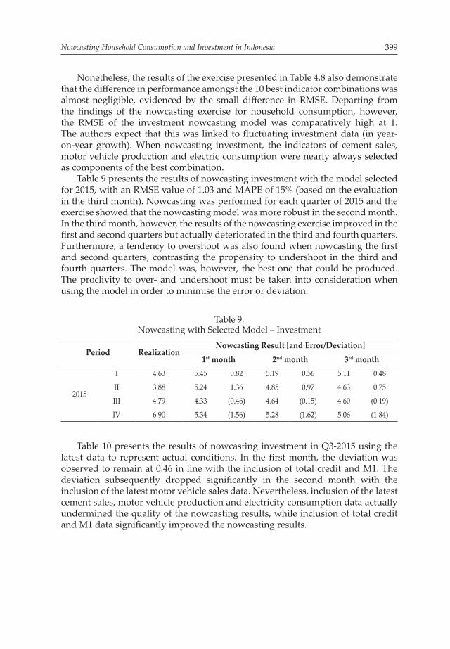
Nowcasting Household Consumption and Investment in Indonesia 399
Nonetheless, the results of the exercise presented in Table 4.8 also demonstrate that the difference in performance amongst the 10 best indicator combinations was almost negligible, evidenced by the small difference in RMSE. Departing from the findings of the nowcasting exercise for household consumption, however, the RMSE of the investment nowcasting model was comparatively high at 1. The authors expect that this was linked to fluctuating investment data (in year-on-year growth). When nowcasting investment, the indicators of cement sales, motor vehicle production and electric consumption were nearly always selected as components of the best combination.
Table 9 presents the results of nowcasting investment with the model selected for 2015, with an RMSE value of 1.03 and MAPE of 15% (based on the evaluation in the third month). Nowcasting was performed for each quarter of 2015 and the exercise showed that the nowcasting model was more robust in the second month. In the third month, however, the results of the nowcasting exercise improved in the first and second quarters but actually deteriorated in the third and fourth quarters. Furthermore, a tendency to overshoot was also found when nowcasting the first and second quarters, contrasting the propensity to undershoot in the third and fourth quarters. The model was, however, the best one that could be produced. The proclivity to over- and undershoot must be taken into consideration when using the model in order to minimise the error or deviation.
Table 9.Nowcasting with Selected Model – Investment
Period RealizationNowcasting Result [and Error/Deviation]
1st month 2nd month 3rd month
2015
I 4.63 5.45 0.82 5.19 0.56 5.11 0.48
II 3.88 5.24 1.36 4.85 0.97 4.63 0.75
III 4.79 4.33 (0.46) 4.64 (0.15) 4.60 (0.19)
IV 6.90 5.34 (1.56) 5.28 (1.62) 5.06 (1.84)
Table 10 presents the results of nowcasting investment in Q3-2015 using the latest data to represent actual conditions. In the first month, the deviation was observed to remain at 0.46 in line with the inclusion of total credit and M1. The deviation subsequently dropped significantly in the second month with the inclusion of the latest motor vehicle sales data. Nevertheless, inclusion of the latest cement sales, motor vehicle production and electricity consumption data actually undermined the quality of the nowcasting results, while inclusion of total credit and M1 data significantly improved the nowcasting results.

Bulletin of Monetary Economics and Banking, Volume 20, Number 3, January 2018400
4.3. Model Performance EvaluationAs mentioned previously, model performance was evaluated by comparing the nowcasting results to the benchmark models, in this case the Bridge Equation and ARIMA model. As presented in Table 11, the comparison of model accuracy for nowcasting household consumption showed that the forecast error of the Dynamic Factor Model was smaller than the forecasting error of the Bridge Equation and
Table 11.Comparison with Other Models – Household Consumption
Nowcasting RealizationNowcasting Result [and Error/ Deviation]
Dynamic Factor Model Bridge Equation ARIMA
2015
I 5.01 5.00 (0.01) 4.33 (0.68) 4.98 (0.03)
II 4.97 4.99 0.03 4.64 (0.33) 4.90 (0.06)
III 4.95 4.96 0.01 4.50 (0.45) 4.88 (0.07)
IV 4.92 4.94 0.01 4.43 (0.50) 4.87 (0.06)
RMSE 0.02 RMSE 0.50 RMSE 0.06
Table 10.Nowcasting Result Based on Data Flow (Q3-2015) – Investment
PeriodData Release
Nowcasting Result[and Error/ Deviation]
RealizationMonth Week
1st month
1 --
4.79
2 Cement salesMotor vehicle productionElectricity consumption
4.33 (0.46)
3 -- 4.33 (0.46)
4 Total creditM1
4.33 (0.46)
2nd month
1 -- 4.33 (0.46)
2 Cement salesMotor vehicle productionElectricity consumption
4.63 (0.16)
3 -- 4.63 (0.16)
4 Total creditM1
4.64 (0.15)
3rd month
1 -- 4.64 (0.15)
2 Cement salesMotor vehicle productionElectricity consumption
4.55 (0.24)
3 -- 4.55 (0.24)
4 Total creditM1
4.60 (0.19)

Nowcasting Household Consumption and Investment in Indonesia 401
ARIMA. Therefore, nowcasting household consumption using the DFM model was shown to be the most robust.
On the other hand, the comparison of model accuracy for nowcasting investment showed that the forecast error of the Dynamic Factor Model was smaller than the forecasting error of the Bridge Equation and ARIMA, as presented in Table 4.12. The forecast error of the DFM model was considered significant but smaller than that of the benchmark models.
Table 12.Comparison with Other Models – Investment
Nowcasting RealizationNowcasting Result [and Error/ Deviation]
Dynamic Factor Model Bridge Equation ARIMA
2015
I 4.63 5.06 0.48 3.10 (1.53) 5.38 0.75
II 3.88 4.73 0.75 3.97 0.09 5.43 1.55
III 4.79 4.63 (0.19) 4.00 (0.79) 4.78 (0.01)
IV 6.90 5.06 (1.84) 4.31 (2.59) 5.68 (1.22)
RMSE 1.03 RMSE 1.55 RMSE 1.06
V. CONCLUSION5.1. Conclusion A number of conclusions can be drawn from the research as follows: 1. The most robust nowcasting models for household consumption and
investment were built using the Dynamic Factor Model (DFM) method based on the various testing and exercise stages. The indicators used for nowcasting household consumption were motor vehicle sales, total deposit, consumer lending rate, M1, and the Rupiah exchange rate (NEER), while the indicators used for nowcasting investment included cement sales, motor vehicle production, electricity consumption, total credit, and M1.
2. Accuracy testing revealed that the forecast error of the household consumption nowcasting model using the DFM method was small and, therefore, robust in terms of predicting the level of household consumption. Meanwhile, the forecast error of the investment nowcasting model using the DFM method was large enough but smaller than the benchmark models (Bridge Equation and ARIMA).
5.2. RecommendationsThe recommendations of the research are as follows:1. Before the nowcasting models for household consumption and investment can
formally be applied to FPAS, further testing is required to observe the accuracy of the nowcasting models for the first two quarters of 2016.
2. Nowcasting models for the other components of GDP should be developed to ensure Bank Indonesia has accurate nowcasting models for all components of GDP.

Bulletin of Monetary Economics and Banking, Volume 20, Number 3, January 2018402
REFERENCEAndersson, Michael K. and Reijer, J.J. den. (2015). Nowcasting. Sveriges Riksbank
Economic Review, No. 2015:1.Andreou, Elena; Ghysels, Eric; and Kourtellos, Andros. (2010). Regression Models
with Mixed Sampling Frequencies. Journal of Econometrics, 158.Angelini, Elena; Camba-Méndez, Gonzalo; Giannone, Domenico; Rünstler,
Gerhard; and Reichlin, Lucrezia. (2008). Short-Term Forecasts of Euro Area GDP Growth.ECB Working Paper Series, No. 949.
Aruoba, S. Boragan; Diebold, Francis X.; and Scotti, Chiara. “Real-Time Measurement of Business Conditions. (2012).Journal of Business and Economic Statistics, No. 27:4.
Baffigi, Alberto; Golinelli, Roberto; and Parigi, Giuseppe. (2004). Bridge Models to Forecast the Euro Area GDP. International Journal of Forecasting, 20.
Bańbura, Marta and Rünstler, Gerhard. (2011). A Look into the Factor Model Black Box: Publication Lags and the Role of Hard and Soft Data in Forecasting GDP.International Journal of Forecasting, 27.
Bańbura, Marta; Giannone, Domenico; and Reichlin, Lucrezia. (2011). Nowcasting. The Oxford Handbook of Economic Forecasting.
Bańbura, Marta; Giannone, Domenico; Modugno, Michele; and Reichlin, Lucrezia. (2012). Now-Casting and the Real-Time Data Flow.ECARES Working Paper, No. 2012-026.
Bell, Venetia; Co, Lai Wah; Stone, Sophie; and Wallis, Gavin. (2014). Nowcasting UK GDP Growth. Bank of England Quarterly Bulletin Q1-2014.
Burns, Arthur F. and Mitchell, Wesley C. Measuring Business Cycles. (1946). New York: NBER.
Camacho, Maximo and Perez-Quiros, Gabriel. (2010). Introducing the Euro-Sting: Short-Term Indicator of Euro Area Growth. Journal of Applied Econometrics, 25(4).
Diebold, Francis X. and Rudebusch, Glenn D. (1996). Measuring Business Cycles: A Modern Perspective. The Review of Economics and Statistics, 78(1).
Doz, Catherine; Giannone, Domenico; and Reichlin, Lucrezia. (2011). A Two-Step Estimator for Large Approximate Dynamic Factor Models Based on Kalman Filtering. Journal of Econometrics, 164.
Foroni, Claudia and Marcellino, Massimiliano. (2013). A Survey of Econometric Methods for Mixed-Frequency Data. Norges Bank Research Working Paper, No. 2013/06.
Ghysels, Eric; Santa-Clara, Pedro; and Valkanov, Rossen. (2004). The MIDAS Touch: Mixed Data Sampling Regression Models.
Giannone, Domenico; Reichlin, Lucrezia; and Small, David. (2008). Nowcasting: The Real-Time Informational Content of Macroeconomic Data.Journal of Monetary Economics, 55.
Hamilton, James D. (1994). State-Space Models in Engle, R.F. and McFadden, D.L. Handbook of Econometrics. Elsevier Science B.V.
Kurniawan, Ferry. (2015). Nowcasting Indonesian Economy. Jakarta: Bank Indonesia.
Luciani, Matteo; Pundit, Madhavi; Ramayandi, Arief; and Veronese, Giovanni. (2015). Nowcasting Indonesia. FRB Finance and Economics Discussion Series, No. 2015-100.

Nowcasting Household Consumption and Investment in Indonesia 403
Mariano, Roberto S. and Murasawa, Yasutomo. (2003). A New Coincident Index of Business Cycles Based on Monthly and Quarterly Series. Journal of Applied Econometrics, 18(4).
Mariano, Roberto S. and Murasawa, Yasutomo. (2010). A Coincident Index, Common Factors, and Monthly Real GDP.Oxford Bulletin of Economics and Statistics, 72(1).
OECD System of Composite Leading Indicators. (2012). OECD.Schorfheide, Frank and Song, Dongho. (2013). Real-Time Forecasting with a
Mixed-Frequency VAR. NBER Working Paper Series, No. 19712.Sørensen, Jonas. (2011). Indicator Models for Private Consumption.Monetary
Review, 1st Quarter 2011.Stock, James H. and Watson, Mark W. (1989). New Indexes of Coincident and
Leading Economic Indicators. Blanchard, Olivier Jean dan Fischer, Stanley (Eds.). NBER Macroeconomics Annual 1989, Volume 4.
The Conference Board. Business Cycle Indicators Handbook. (2001).

This page is intentionally left blank
Bulletin of Monetary Economics and Banking, Volume 20, Number 3, January 2018404

Bulletin of Monetary Economics and Banking, Volume 20, Number 3, January 2018 405
MANUSCRIPT GUIDANCE
1. Manuscript must be an original work of the author (individuals, groups or institutions) that do not infringe copyright. The submitted manuscript has never been published nor being sent to other publishers. The copyright of the received manuscript shall be kept by the author.
2. Manuscript shall be sent in soft file to website BMEB: (www.journalbankindonesia.org)and email : [email protected].
3. Manuscript is written to maximum of 25 pages of A4 size, with single space (1), “Times New Roman” and 12 font size.
4. Mathematical equations and symbols shall be written using Microsoft Equation.
5. Title of the manuscript shall be in English.6. Each manuscript shall have Abstraction in English to maximum of one page
(1) of A4 size.7. Manuscript shall have keyword and two-digit classification number of Journal
of Economic Literature (JEL). Please see the JEL Classification at http://www.aeaweb.org/journal/jel_class_system.html.
8. Chapter in the manuscript shall be written in a consistent way as follows : I. CHAPTER TITLE I.1. SUB CHAPTER I.1.1. SUB SUB CHAPTER9. References shall be written using footnote, not endnote.10. The references system is built on this following rules :
a. Book Publication Hanke, J. E., & Reitsch, A. G. (1940). Business Forecasting. New Jersey:
Prentice Hall.b. Article in Journal Rangazas, P. (2000). Schooling and Economic Growth: A King-Rebelo
Experiment with Human Capital. Journal of Monetary Economics, 46(2), 397–416.
c. Working papers Kremer, M., & Chen, D. (2000). Income Distribution Dynamics with
Endogenous Fertility (National Bureau of Economic Research (Cambridge, MA) Working Paper No. 7530).
d. Articles from websites and other electronic forms Robert, S., & Henston, A. W. (1997). Penn World Table Version 5.6. Retrieved
January 10, 2001, from http://pwt.econ.upenn.edu/.e. Articles in newspaper, magazine and periodicals or similar periodicals Begley, S. (1993, April 12). Killed by Kindness. Newsweek, pp. 50–56. New
York.

Bulletin of Monetary Economics and Banking, Volume 20, Number 3, January 2018406
f. Proceeding World Economic Forum. (2016). Global Competitiveness Index 2016-2017.
Geneva.g. Report (unpublished) Engle, R. ., & Lee, G. J. (1993). A Permanent and Transitory Component Model
of Stock Return Volatility. Discussion Paper. San Diego.11. Manuscript should be submitted along with author’s biography with a complete
postal address, telephone number and email address. It is recommended to write a author’s bio data in complete Curriculum vitae (CV).