Volume 12 Number 4 Scale Coarseness as a 2009 SAGE ... · PDF filetions as well as the...

Scale Coarseness as aMethodological Artifact

Correcting Correlation Coefficients

Attenuated From Using Coarse Scales

Herman AguinisUniversity of Colorado Denver

Charles A. PierceUniversity of Memphis

Steven A. CulpepperMetropolitan State College of Denver

Scale coarseness is a pervasive yet ignored methodological artifact that attenuates observed

correlation coefficients in relation to population coefficients. The authors describe how to

disattenuate correlations that are biased by scale coarseness in primary-level as well as meta-

analytic studies and derive the sampling error variance for the corrected correlation. Results

of two Monte Carlo simulations reveal that the correction procedure is accurate and show the

extent to which coarseness biases the correlation coefficient under various conditions (i.e.,

value of the population correlation, number of item scale points, and number of scale items).

The authors also offer a Web-based computer program that disattenuates correlations at the

primary-study level and computes the sampling error variance as well as confidence intervals

for the corrected correlation. Using this program, which implements the correction in pri-

mary-level studies, and incorporating the suggested correction in meta-analytic reviews will

lead to more accurate estimates of construct-level correlation coefficients.

Keywords: scale coarseness; Likert-type scale; correlation coefficient; meta-analysis; artifact

Proponents of psychometric approaches to meta-analysis extend arguments from mea-

surement theory to contend that effect sizes such as correlation coefficients are often

underestimated in primary-level studies because of the operation of methodological and

Authors’ Note: A previous version of this article was presented at A Perfect and Just Weight, A Perfect and

Just Measure (J. M. Cortina, Chair), a symposium conducted at the meeting of the Society for Industrial and

Organizational Psychology, New York, April 2007. We thank Roger B. Rensvold for useful conversations

and exchanges of ideas at the outset of this project, Philip Bobko and Frank L. Schmidt for comments on pre-

vious drafts, and Michael C. Sturman for comments on previous drafts and suggestions regarding the design

of the Monte Carlo simulations. This research was conducted, in part, while Herman Aguinis was on sabbati-

cal leave from the University of Colorado Denver and holding visiting appointments at the University of Sala-

manca (Spain) and University of Puerto Rico. Also, this research was supported by a grant from the Center for

International Business Education and Research (CIBER) at the University of Colorado Denver Institute for

International Business. Please address correspondence to Herman Aguinis, Mehalchin Term Professor of Man-

agement, The Business School, University of Colorado Denver, Campus Box 165, P.O. Box 173364, Denver,

CO 80217; http://carbon.cudenver.edu/∼haguinis/

623

Organizational

Research Methods

Volume 12 Number 4

October 2009 623-652

� 2009 SAGE Publications

10.1177/1094428108318065

http://orm.sagepub.com

hosted at

http://online.sagepub.com

by Herman Aguinis on September 23, 2009 http://orm.sagepub.comDownloaded from


statistical artifacts (e.g., Aguinis & Pierce, 1998; Aguinis, Sturman, & Pierce, 2008;

Schmidt, 2008). Hunter and Schmidt (2004) provided a description of the 11 known meth-

odological artifacts (e.g., sampling error, measurement error, direct range restriction) that

reduce the magnitude of observed correlations in relation to their population counterparts.

Because methodological artifacts have a large impact on the magnitude of estimated cor-

relations, there is ongoing interest in the organizational sciences in the biasing effects of

methodological artifacts as well as how to minimize these biases (e.g., Le, Oh, Shaffer, &

Schmidt, 2007; Schmidt, Oh, & Le, 2006). Perhaps just as important, the organizational

sciences, like any other scientific field, need to continue to improve the accuracy of mea-

surements and estimations of theoretically important parameters (Aguinis, 2001; Schmidt

et al., 2006). This need provides the impetus for the ongoing interest in procedures for

estimating parameters such as correlation coefficients more accurately (e.g., see Hunter,

Schmidt, & Le, 2006).

In this article, we address a methodological artifact that can produce a downward bias

in observed correlations but has thus far received virtually no attention in the organiza-

tional sciences: scale coarseness. This is an important problem for the organizational

sciences and related fields because, although this biasing artifact remains largely unac-

knowledged, in many situations researchers may have underestimated construct-level

correlations because of scale coarseness.

Our article is organized as follows. First, we describe scale coarseness and its effects on

the correlation coefficient and we discuss implications of scale coarseness for organiza-

tional science theory and practice. Second, we describe a method that corrects for the

downward biasing effect of scale coarseness. Third, we describe results of two Monte

Carlo simulations that examine the accuracy of the correction procedure and the extent to

which scale coarseness attenuates the correlation coefficient under various conditions (i.e.,

value of the population correlation, number of item scale points, and number of scale

items). Fourth, we derive the currently unknown sampling error variance and confidence

intervals for the corrected correlation. Fifth, we offer a user-friendly, Web-based compu-

ter program that enables researchers to implement the correction for individual correla-

tions as well as the computation of sampling error and confidence intervals for the

corrected correlation. Finally, we describe a new procedure for incorporating the scale

coarseness correction in a meta-analysis. In short, the goals of this article are to: (a) iden-

tify scale coarseness as a pervasive and important, yet often ignored, methodological arti-

fact in organizational science research; (b) demonstrate the biasing effects of scale

coarseness under various conditions; and (c) provide a solution to mitigate these biasing

effects in future primary-level as well as meta-analytic research. As noted by Vandenberg

(2008), our goal is to address an issue that has ‘‘immediate applicability to researchers

both methodologically and empirically’’ (p. 7).

Scale Coarseness

A measurement scale is coarse when a construct that is continuous in nature is mea-

sured using items such that different true scores are collapsed into the same category. In

these situations, errors are introduced because continuous constructs are collapsed or

624 Organizational Research Methods



crippled (Bollen & Barb, 1981). Although this fact is seldom acknowledged, organiza-

tional science researchers use coarse scales every time continuous constructs are measured

using Likert-type (Bollen & Bard, 1981) or ordinal (O’Brien, 1979) items.1 We are so

accustomed to using these types of items that we seem to have forgotten they are intrinsi-

cally coarse. As noted by Blanton and Jaccard (2006), ‘‘scales are not strictly continuous

in that there is coarseness due to the category widths and the collapsing of individuals with

different true scores into the same category. This is common for many psychological mea-

sures, and researchers typically assume that the coarseness is not problematic’’ (p. 28).

As an illustration, consider a typical Likert-type item including 5 scale points or

anchors ranging from 1 (strongly disagree) to 5 (strongly agree). When one or more

Likert-type items are used to assess continuous constructs, such as job satisfaction, per-

sonality, organizational commitment, and job performance, information is lost because

individuals with different true scores are considered to have identical standing regarding

the underlying construct. Specifically, all individuals with true scores around 4 are

assigned a 4, all those with true scores around 3 are assigned a 3, and so forth. However,

differences may exist between these individuals’ true scores (e.g., 3.60 vs. 4.40 or 3.40 vs.

2.60, respectively), but these differences are lost due to the use of coarse scales because

respondents are forced to provide scores that are systematically biased downwardly or

upwardly. This information loss produces a downward bias in the observed correlation

coefficient between a predictor X and a criterion Y. In short, scales that include Likert-type

and ordinal items are coarse, imprecise, do not allow individuals to provide data that are

sufficiently discriminating, and yet they are used pervasively in the organizational

sciences to measure constructs that are continuous in nature. This is unfortunate, given

that cognitive psychologists and psychometricians have concluded that humans are able to

provide data with greater degree of discrimination and precision by using scales with as

many as 20 (Garner, 1960) or 25 (Guilford, 1954) points.

Unique Bias Introduced by Scale Coarseness

Scale coarseness creates a form of nonlinear and systematic error (Symonds, 1924) and

creates a bias that is distinct from the effects of random measurement error and the dichot-

omization of predictor and/or criterion variables. Next, we discuss the relationship

between scale coarseness and (a) measurement error and (b) dichotomization.

Scale coarseness and measurement error. Scale coarseness and random measurement

error are both impossible to correct at the individual level. However, the random error cre-

ated by lack of perfect reliability of measurement is different in nature from the systematic

error introduced by scale coarseness, so these artifacts are distinct and should be consid-

ered separately. Based on classic measurement theory, Xt =Xo + e, where Xt is the true

score, Xo is the observed score, and e is the error term, which is composed of a random

and a systematic (i.e., bias) component (i.e., e= er + es). For example, consider an indivi-

dual who has a true score of 4.4 on the latent construct ‘‘trust in your supervisor’’ (i.e.,

Xt = 4:4). A measure of this construct is not likely to be perfectly reliable, so if we use a

multi-item Likert-type scale, Xo is likely to be greater than 4.4 for some of the items and

less than 4.4 for some of the other items, given that er can be positive or negative because

Aguinis et al. /Scale Coarseness 625



of its random nature. On average, the greater the number of items in the measure, the more

likely it is that positive and negative er values will cancel out and Xo will be closer to 4.4.

So, the greater the number of items for this scale, the less the detrimental impact of ran-

dom measurement error on the difference between true and observed scores; this is an

important reason why multi-item scales are preferred over single-item scales.

Now, in sharp contrast to the measurement error discussion above, let’s consider the

scale coarseness artifact. If we use a scale with only one Likert-type item with, for exam-

ple, 5 scale points, Xo is systematically biased downwardly because this individual respon-

dent will be forced to choose 4 as his response (i.e., the closest to Xt = 4:4) given that 1, 2,

3, 4, and 5 are the only options available. If we add another item and the scale now

includes 2 items instead of only one, the response on each of the 2 items will be biased

systematically by −.4 due to scale coarseness. So, in contrast to the effects of measure-

ment error, the error caused by scale coarseness is systematic and the same for each item.

Consequently, increasing the number of items does not lead to a canceling out of error.

Similarly, an individual for whom Xt = 3:7 will also choose the option 4 on each of the

items for this multi-item Likert-type scale (i.e., the closest to the true score, given that 1,

2, 3, 4, and 5 are the only options available). So, regardless of whether the scale includes

one or multiple items, information is lost due to scale coarseness and these two individuals

with true scores of 4.4 and 3.7 will appear to have an identical score of 4.0.

As noted eloquently by Russell and Bobko (1992) within the specific context of detect-

ing interaction effects, but equally applicable to any other situation in which scales are

coarse,

summing responses to multiple Likert-type items on a dependent scale (as is often done in

between-subjects survey designs) is not the same as providing subjects with a continuous

response scale. Although the resultant ‘‘scale score’’ obtained by summing item responses

could be considered nearly continuous, subjects are not responding with a scale score.

Rather, they are responding to each item individually. Thus, if an individual responds to

coarse Likert scales in a similar manner across items, the problem of reduced power to detect

interaction remains. . . information loss that causes systematic error to occur at the item level

would have the same effect on moderated regression effect size regardless of whether the

dependent-response items were analyzed separately (as was done here in a within-subject

design) or cumulated into a scale score. (p. 339)

Evidence accumulated over the past half a century supports the argument that scale

coarseness and measurement error have independent effects in most situations. For exam-

ple, Bendig (1953) provided evidence that the number of scale points is independent of

the scale’s reliability. Specifically, study participants rated their knowledge of 12 different

countries using items with either 3, 5, 7, 9, or 11 scale points. Results showed that reliabil-

ity estimates were relatively constant with a slight drop in reliability for the 11 scale-point

condition. In a follow-up study, Bendig (1954) also provided evidence regarding the lack

of relationship between scale coarseness and reliability. In that study, 236 participants

rated a list of 20 foods (i.e., a 20-item scale) using items with 2, 3, 5, 7, or 9 scale points.

Thus, in contrast to Bendig (1953), Bendig (1954) used a multi-item scale. He concluded

that ‘‘The results regarding test reliability are fairly unequivocal. No consistent trend was

found in the relation of test reliability and number of scale categories’’ (p. 39). Moreover,




‘‘test reliability was constant over the entire range of categories and was very similar to

reliabilities found in another study. . .. It was concluded that test reliability is independent

of the number of scale categories’’ (p. 40).

About 10 years later, Komorita and Graham (1965) collected data from 260 students

using two different scales (i.e., Semantic Differential adjectives and California Psycholo-

gical Inventory), which vary regarding item homogeneity. Also, they manipulated the

number of item scale points by using either 2 or 6. The conclusion was:

With a relatively homogeneous set of items, the reliability of a scale is independent of the

number of item scale-points. If the items are relatively heterogeneous, however, the results

suggest that the reliability of the scale can be increased not only by increasing the number of

items but also by increasing the number of item scale-points. (p. 993)

Also, he argued that ‘‘based on the evidence adduced thus far, it would seem that reliabil-

ity should not be a factor considered in determining Likert-scale rating format, as it is

independent of the number of scale steps employed’’ (p. 670).

In a more detailed examination of the effects of scale coarseness, Mattell and Jacoby

(1971) used 18 different groups of 20 students each, who were assigned to experimental

conditions varying in terms of number of scale points (i.e., from 2 to 19). In contrast to

previous investigations, Mattell and Jacoby computed not only internal consistency but

also stability (i.e., test-retest) reliability estimates. The conclusion was that ‘‘both reliabil-

ity measures, test-retest and internal consistency, were found to be independent of the

number of scale-points’’ (p. 666).

Finally, Aiken (1983) administered a teaching evaluation instrument consisting of a

multi-item scale with 10 items to 624 undergraduate students in freshman-level courses.

He varied scale coarseness by using the same items but varying the number of scale points

from 2 to 7. He concluded that ‘‘although increased variance is usually associated with

increased reliability, such was not the case in this investigation’’ (p. 400). The internal

consistency reliability estimates (alphas) showed no systematic change associated with

various levels of scale coarseness. Accordingly, Aiken (1983) concluded that ‘‘the fact

that the internal consistency reliability coefficients remained relatively constant despite

the increase in response variance indicates that efforts to increase the spread of responses

by employing a greater number of response categories will not necessarily improve scale

reliability’’ (p. 401).

In sum, the effect of measurement error is random and increasing the number of items

decreases the impact of the measurement error artifact on the difference between popula-

tion and observed correlations. In contrast, the effect of scale coarseness is systematic and

increasing the number of items does not necessarily decrease its impact on loss of infor-

mation due to the collapsing of different true scores within the same category. In addition,

evidence accumulated thus far supports the conclusion that, in most situations, scale coar-

seness and measurement error have independent effects.

Scale coarseness and dichotomization. The scale coarseness artifact is also distinct

from the dichotomization of predictor and/or criterion variables artifact. Scale coarseness

is an artifact that is introduced when data are collected and is due to the nature of the




measurement instrument used and, therefore, it is a research design artifact. In contrast,

the dichotomization artifact is introduced after data are collected and then scores are split

(e.g., at the median) creating ‘‘high’’ and ‘‘low’’ categories (Cohen, 1983), so dichotomi-

zation is a data-analysis artifact. In other words, the bias created by scale coarseness is not

related to the bias created by dichotomization, and the presence or absence of scale coar-

seness is not related to the presence or absence of dichotomization. For example, assume

a situation in which there is severe scale coarseness and both the predictor and criterion

variables are measured using 3 scale points each (e.g., below average, average, and above

average anchors). In this situation, a researcher would apply the scale coarseness correc-

tion to the observed correlation coefficient. In addition, prior to computing the correlation

coefficient, a researcher may have chosen to split the data into the following two groups

based on the criterion scores: (a) individuals scoring above the median and (b) individuals

scoring below the median. In this situation, one would apply the dichotomization correc-

tion to the observed correlation because the criterion scores were artificially dichotomized.

If, on the other hand, the sample is not split into these high and low subgroups, then one

would not apply the dichotomization correction but would still apply the scale coarseness

correction. In sum, scale coarseness is a research design-based artifact, whereas dichoto-

mization is a data-analysis-based artifact and, hence, they are independent of each other

and should be considered separately (cf. Hunter & Schmidt, 2004, pp. 112-115).2

Effects of Scale Coarseness on Correlation Coefficients:

Implications for Organizational Science Research

The lack of precision introduced by coarse scales has a downward biasing effect on the

correlation coefficient computed using data collected from such scales for the predictor,

the criterion, or both variables. For example, consider the case of a correlation computed

based on measures that use items anchored with 5 scale points. In this case, a population

correlation of .50 is attenuated to a value of .44 (we describe the correction procedure later

in the article).3 A difference between correlations of .06 indicates that the correlation is

attenuated by about 14%.

The above is a realistic yet hypothetical example. Are the implications of scale coarse-

ness actually meaningful? To answer this question, we first note that scale coarseness is a

pervasive phenomenon across a variety of organizational science domains, given that the

use of coarse measures including as few as 5, 4, or even 3 scale points is quite common.

In fact, this type of operationalization of continuous constructs is ordinary practice in most

organizational science domains because of the popularity of Likert-type scales. We

reached this conclusion after reviewing recent issues of Academy of Management Journal

(AMJ), Journal of Management (JoM), Journal of Applied Psychology (JAP), and Person-

nel Psychology (PPsych), in which we had no difficulty finding numerous articles in each

issue that used coarse scales to assess continuous constructs (see Table 1 for examples).

To provide a more precise answer to the question of whether the implications of scale

coarseness are meaningful, we assessed the underestimation in correlation coefficients, and

coefficients of determination (r2), in the recently published literature (we describe the cor-

rection procedure in detail later in the article). Specifically, we reviewed articles published




Tab

le1

Sel

ecti

ve

Lit

eratu

reR

evie

wA

sses

sin

gth

eIm

pact

of

Sca

leC

oars

enes

son

the

Un

der

esti

mati

on

of

the

Coef

fici

ent

of

Det

erm

inati

on

(r2)

Stu

dy

Pre

dic

tor

Cri

teri

on

Rep

ort

ed

r(r

2)

Corr

ecte

d

r(r

2)

Under

esti

mat

ion

inr2

(%)

All

enet

al.

(2006)

Men

tor

com

mit

men

tP

rogra

mef

fect

iven

ess

.38

(.14)

.43

(.18)

28

Bar

rick

etal

.(2

007)

Tea

min

terd

epen

den

ceT

eam

per

form

ance

.17

(.03)

.19

(.04)

25

Bro

wn

etal

.(2

006)

Sel

f-ef

fica

cyJo

bse

arch

beh

avio

r.1

3(.

02)

.15

(.02)

33

Cra

mto

net

al.(2

007)

Tas

kco

hes

ion

Sat

isfa

ctio

nw

ith

team

.18

(.03)

.20

(.04)

24

Die

rdorf

f&

Surf

ace

(2007)

Soci

alin

tera

ctio

nT

acti

cal

pro

fici

ency

.71

(.50)

.80

(.64)

27

Fed

or

etal

.(2

006)

Job

level

chan

ge

Org

aniz

atio

nal

com

mit

men

t−.

13

(.02)

−.15

(.02)

33

Fer

rin

etal

.(2

006)

Cow

ork

erci

tize

nsh

ipE

mplo

yee

trust

.47

(.22)

.53

(.28)

27

Fong

&T

osi

(2007)

Consc

ienti

ousn

ess

Agre

eable

nes

s.1

3(.

02)

.15

(.02)

33

Geo

rge

&Z

hou

(2007)

Posi

tive

mood

Cre

ativ

ity

.25

(.06)

.28

(.08)

25

Gri

ffin

etal

.(2

007)

Tea

mpro

acti

vit

yO

rgan

izat

ion

pro

acti

vit

y.7

9(.

62)

.89

(.79)

27

Kle

inet

al.

(2007)

Goal

ori

enta

tion

Moti

vat

ion

tole

arn

.22

(.05)

.25

(.06)

29

Lam

etal

.(2

007)

Impre

ssio

nm

oti

ves

Lea

der

–m

ember

exch

ange

−.04

(.00)

−.05

(.00)

56

Mar

cus

etal

.(2

007)

Agre

eable

nes

sU

.S.over

tin

tegri

ty.2

5(.

06)

.28

(.08)

25

Mar

ler

etal

.(2

006)

Eas

eof

use

Inte

nt

touse

tech

nolo

gy

.27

(.07)

.29

(.08)

15

McK

ayet

al.

(2007)

Div

ersi

tycl

imat

eT

urn

over

inte

nti

ons

−.26

(.07)

−.29

(.08)

24

Meg

lino

&K

ors

gaa

rd(2

007)

Pre

vio

us

job

attr

ibute

sR

ecen

tjo

bat

trib

ute

s.1

5(.

02)

.16

(.03)

14

Rogel

ber

g,

Lea

chet

al.(2

006)

Tas

kin

terd

epen

den

ceIn

tenti

ons

toquit

−.08

(.01)

−.10

(.01)

56

Vec

chio

&B

razi

l(2

007)

Per

form

ance

Sat

isfa

ctio

nw

ith

lead

er.1

0(.

01)

.11

(.01)

21

Wri

ght

&B

onet

t(2

007)

Job

sati

sfac

tion

Psy

cholo

gic

alw

ell-

bei

ng

.37

(.14)

.40

(.16)

17

Note

:F

or

under

esti

mat

ion

inr2

,M

ean

(SD

)=

29%

(11%

).F

or

under

esti

mat

ion

inr,

Mea

n(S

D)=

13%

(5%

).

629



in 2006 and 2007 in AMJ, JoM, JAP, and PPsych. We acknowledge that this is not an

exhaustive or even a comprehensive review. Such a review would include the vast majority

of articles ever published in these journals given the pervasiveness of Likert-type scales in

organizational science research. Instead, in our review we selected a few articles a priori

without looking at the correlations reported or the number of scale points used in the mea-

sures. Articles we found include coarse measures of team cohesion, team communication,

and team interdependence (Barrick, Bradley, Kristof-Brown, & Colbert, 2007); mood states

at work (George & Zhou, 2007); team member and organization member proactivity (Grif-

fin, Neal, & Parker, 2007); supervisor-attributed impression management motives and qual-

ity of leader–member exchange (Lam, Huang, & Snape, 2007); job satisfaction and

psychological well-being (Wright & Bonett, 2007); conscientiousness (Fong & Tosi, 2007);

accuracy of recent and previous job attributes (Meglino & Korsgaard, 2007); intention to

use technology (Marler, Liang, & Dulebohn, 2006); interpersonal organizational citizenship

behaviors, employee trust in coworkers, and interpersonal communication (Ferrin, Dirks, &

Shah, 2006); task interdependence (Rogelberg, Leach, Warr, & Burnfield, 2006); job search

self-efficacy (Brown, Cober, Kane, Levy, & Shalhoop, 2006); personality and integrity

(Marcus, Lee, & Ashton, 2007); organizational commitment, diversity climate perceptions,

and turnover intentions (McKay et al., 2007); peer ratings of performance (Dierdorff & Sur-

face, 2007); learning goal orientation and motivation to learn (Klein, Noe, & Wang, 2007);

job level change and change commitment (Fedor, Caldwell, & Herold, 2006); and mentor

commitment and perceived program effectiveness (Allen, Eby, & Lentz, 2006), among

others. Thus, related to our earlier assertion regarding the pervasiveness of the scale coarse-

ness artifact, it seems it would be difficult to name an area within the organizational sciences

in which the scale coarseness artifact has not produced downwardly biased estimates of how

well a predictor relates to a criterion.

Table 1 summarizes results of our review. Scale coarseness caused an average underes-

timation in r of about 13% and an average underestimation in r2 of about 30%. In other

words, on average, scale coarseness led researchers to conclude that their predictor

explains about 30% less of the variance in their criterion than is actually the case. So, the

underestimation is meaningful. But, is it nontrivial and can it lead to incorrect inferences?

We provide four different types of arguments and evidence to answer this question in the

affirmative.

First, an attenuation in the correlation coefficient between 10% to 20% is comparable

to, and in some cases larger than, the percent of attenuation typically caused by measure-

ment error (e.g., Bowling & Beehr, 2006; Halbesleben, 2006) and range restriction

(Hunter et al., 2006) in some organizational science domains. Besides sampling error,

measurement error and range restriction are the two methodological artifacts most fre-

quently studied in the organizational sciences and are also the two methodological arti-

facts for which meta-analysts correct most frequently (Hunter & Schmidt, 2004).

We reviewed recent issues of several organizational science journals to compare the rela-

tive impact of the measurement error and scale coarseness artifacts on estimates of the cor-

relation coefficient. Consider the case of the relationship between subordinates’ degree of

coaching guidance and degree of social support from supervisor (Heslin, Vandewalle, &

Latham, 2006). Coaching guidance, which is a continuous construct, was measured using a

5-point agreement scale with anchors ranging from 1 (not at all) to 5 (to a very great




extent). The internal consistency reliability estimate for this scale was .92. Social support

was also measured using a 5-point scale with anchors ranging from 0 (don’t have any such

person) to 4 (very much) and this scale’s reliability was .79. The observed correlation

between coaching guidance and support was .46. Applying the measurement error correc-

tion to both variables to obtain the disattenuated correlation (i.e., rxy=½ffiffiffiffiffiffirxxp ffiffiffiffiffi

ryyp �) leads to a

value of .54. Alternatively, using the scale coarseness correction (which we describe in more

detail later in this article) leads to a comparable value of .52. As a second recent illustration,

consider the case of the relationship between data usage/good use of surveys, measured on a

5-point scale ranging from 1 (strongly disagree) to 5 (strongly agree; reliability= .87), and

attitudes toward (i.e., like) filling out surveys, also measured using a 5-point scale ranging

from 1 (strongly disagree) to 5 (strongly agree; reliability= .92; Rogelberg, Spitzmueller,

Little, & Reeve, 2006). The corrected correlation based on measurement error on both the

predictor and the criterion leads to a corrected value of .34, and applying the scale coarse-

ness correction also leads to a value of .34. Given the accumulated knowledge regarding the

detrimental effects of artifacts such as measurement error on estimates of correlation coeffi-

cients (Schmidt & Hunter, 1996), it would be incorrect to argue that the measurement error

correction should not be implemented because the biasing effect of measurement error is

‘‘too small.’’ Accordingly, if scale coarseness causes a degree of attenuation comparable to

the attenuation caused by measurement error, then scale coarseness should also be consid-

ered a nontrivial methodological artifact.

Second, attenuations in the 10% to 20% range are larger than the percentage improve-

ment in the estimation of the sampling error variance of the correlation coefficient caused

by taking into account indirect range restriction (Aguinis & Whitehead, 1997) and an

improved formula (Aguinis, 2001). Thus, if improvements in the estimation of sampling

error variance in the correlation coefficient in the 5% to 10% range are considered suffi-

ciently important for substantive conclusions in organizational science research (Aguinis,

2001; Aguinis & Whitehead, 1997), then improvements in the estimation of the correla-

tion coefficient in the 10% to 20% range should also be taken seriously.

Third, we argue that, in some research domains, an underestimation in r in the order of

10% to 20% can lead to imprecise inferences. An underestimation in r of about 13% may

be seen as a small effect. However, it is generally not appropriate to equate Cohen’s (1988)

definitions of small and large effects with unimportant effect and important effect, respec-

tively, without taking into account the research context and domain in question (Aguinis,

Beaty, Boik, & Pierce, 2005; Aguinis & Harden, in press). Cohen (1988) noted that ‘‘the

terms ‘small,’ ‘medium,’ and ‘large’ are relative, not only to each other, but to the area of

behavioral science or even more particularly to the specific content and research method

being employed in any given investigation’’ (p. 25). Specifically, in some contexts, what

may be labeled as a ‘‘small’’ effect using Cohen’s definitions can actually have important

consequences for organizational science theory and practice. For example, consider the

result reported in Table 1 that the underestimation in r2 is, on average, about 30%, in the

context of research on diversity and performance management. Martell, Lane, and Emrich

(1996) found that an effect size of 1% regarding male–female differences in performance

appraisal scores led to only 35% of the highest-level positions being filled by women.

Accordingly, Martell et al. (1996) concluded that ‘‘relatively small sex bias effects in

performance ratings led to substantially lower promotion rates for women, resulting in




proportionately fewer women than men at the top levels of the organization’’ (p. 158).

Another relevant example in the organizational sciences is the area of staffing decision mak-

ing. For example, the algorithms and program developed by Aguinis and Smith (2007) show

that differences in correlations that are as small as .03 across ethnicity-based subgroups are

sufficiently large to cause important changes in the resulting adverse impact and false posi-

tive and false negative ratios. These are important outcomes that change based on whether

the scales are coarse. In sum, the difference between the attenuated and disattenuated (by

scale coarseness) correlation has important implications for organizational science theory

and practice in several domains (for an additional illustration of the practical impact of what

may seem ‘‘small’’ differences between correlations, see Schmidt, Hunter, McKenzie, &

Muldrow, 1979). The underestimation caused by scale coarseness can lead researchers to

make incorrect inferences from their findings, such as concluding that male–female differ-

ences in performance appraisal scores do not affect the career progression of women, and

that a selection test is not likely to lead to adverse impact. Perhaps just as noteworthy is that

an important hallmark of any scientific field is continuous improvement in accuracy of mea-

surements and estimations of theoretically important parameters (Aguinis, 2001; Schmidt

et al., 2006). Taking into account scale coarseness will contribute to improved accuracy in

the estimation of population correlation coefficients.

Finally, an additional important issue to consider in terms of making incorrect infer-

ences is the biasing effect of scale coarseness on meta-analytically derived correlation

coefficients. Results of validity generalization studies involving continuous constructs

measured using coarse scales are likely to have underestimated the resulting mean validity

coefficient. For example, Judge, Heller, and Mount’s (2002) meta-analysis of the relation-

ship between overall job satisfaction and the five-factor model of personality likely under-

estimated population correlations because most of the studies included in this meta-

analysis used coarse scales to measure job satisfaction.

In sum, we have provided evidence in support of the conclusion that the implications of

scale coarseness are meaningful, nontrivial, and can result in making imprecise inferences.

Next, we discuss a procedure for correcting the downward bias introduced by scale coar-

seness in primary-level studies. Then, we describe results of two Monte Carlo simulations

that examine the accuracy of the correction procedure and conditions under which the

effects of scale coarseness are most pronounced. After reporting results of the simulations,

we offer a new procedure for computing sampling error variance and confidence intervals

for the resulting corrected correlation. Also, we describe a user-friendly, Web-based com-

puter program that enables the implementation of this correction procedure at the primary

level, including the computation of sampling error variance and confidence intervals for

the corrected correlation. Finally, we describe a new procedure for incorporating a scale

coarseness correction procedure in conducting a meta-analysis.

Correcting for the Downward Bias Introduced by Scale Coarseness

As is the case with other statistical and methodological artifacts that produce a downward

bias in the correlation coefficient, elimination of the methodological artifact via research

design before data are collected ‘‘is vastly superior to elimination by statistical formula after




the fact’’ (Hunter & Schmidt, 2004, p. 98). Thus, as implemented by Arnold (1981) and

Russell and Bobko (1992; Russell, Pinto, & Bobko, 1991), and suggested by others (Krieg,

1999), one possibility regarding the measurement of continuous constructs is to use a con-

tinuous graphic rating scale (i.e., a line segment without scale points) instead of Likert-type

scales. Then, a researcher can measure the distance (e.g., in millimeters) from the left side of

the line segment to the individual’s response point, thereby resulting in a nearly-continuous

measure (Arnold, 1981; Russell & Bobko, 1992; Russell et al., 1991). However, this type of

data collection procedure is not practically feasible in most situations unless data are collected

electronically (Aguinis, Bommer, & Pierce, 1996).

Because using continuous graphic rating scales is often difficult to implement in practice

and because there are so many established operationalizations of truly continuous constructs

using Likert-type scales, the next best solution to address the downward bias produced by

scale coarseness is to implement a statistical correction after data are collected. This correc-

tion was derived by Peters and van Voorhis (1940, pp. 396-397) by solving for the disatte-

nuated relationship between X and Y in terms of the attenuated/observed correlation using

partial correlation formulas. They benefited from recognizing that the relationship between

a categorical X and continuous Y controlling for the continuous X equals zero and employed

Sheppard’s correction to the coarse variance (Sheppard, 1897, 1907). Peters and van Voor-

his’s (1940) correction factors assume a linear relationship between X and Y, equally spaced

intervals for the categorical X and Y (e.g., coding a 3-point scale as 1, 2, and 3, or 0, 1, and

2), and a finite space on the latent continuum (i.e., they calculated their correction factors by

creating intervals of standardized scores between -3 and 3).

The correction procedure for scores assumed to be normally distributed in the popula-

tion is accurate even when the distributions for the predictor and criterion scores are

severely skewed unless one or both variables are measured using a binary scale (Wylie,

1976). For example, Martin (1978) tested the Peters and van Voorhis correction procedure

and found that corrected correlations of .81 and .49 were almost identical to their popula-

tion counterparts of .80 and .50, respectively. Based on the results of his Monte Carlo

simulations, Martin (1978) concluded that ‘‘the corrected rs are for pragmatic purposes

the same as the ‘true’ rs’’ and he also concluded that ‘‘the correction factors are valuable,

but they are rarely used’’ (p. 307).

Unfortunately, as noted by Martin (1978), researchers do not seem to be aware of this cor-

rection procedure. This is particularly true for researchers in the organizational sciences. We

reached this conclusion after conducting an extensive literature search of all articles that

cited Peters and van Voorhis (1940). We conducted our search using Web of Science,

including the Science Citation Index Expanded and the Social Sciences Citation Index, from

January 1965 to July 2007. This search resulted in 195 citations of Peters and van Voorhis

(1940). None of these citations were from articles published in premier management jour-

nals such as Academy of Management Journal, Journal of Management, Strategic Manage-

ment Journal, and Administrative Science Quarterly. Three of these citations were for

articles published in PPsych (Buel, 1969; Carlson, 1969; Taylor & Griess, 1976); 6 were for

articles published in JAP (Ash, 1971; Buel, 1965; Carlson, 1967; Kemery, Dunlap, & Grif-

feth, 1988; Russell & Bobko, 1992; Williams, 1990); and 1 each for Organizational

Research Methods (ORM; Edwards, 2001); Journal of Organizational Behavior (JOB;

Corrigan et al., 1994); Sloan Management Review (SMR; Gross, 1972); and Organizational




Behavior and Human Performance (OBHP; Andrews & Farris, 1972). Each of the PPsych,

ORM, JOB, SMR, and OBHP and three of the six JAP articles (Buel, 1965; Carlson, 1967;

and Kemery et al., 1988) cited sections of the Peters and van Voorhis book that do not

address the topic of scale coarseness. Two other JAP articles (Russell & Bobko, 1992, and

Williams, 1990) cited Peters and van Voorhis to support the general statement that scale

coarseness produces a downward bias on the correlation coefficient, but neither article men-

tioned the existence of a correction procedure that would address this bias. Finally, Ash

(1971) noted in one sentence in the article’s Results section that ‘‘since the recommended-not

recommended judgment may be considered a continuous variable, a Pearson product-moment

correlation, corrected for broad categories (Peters & van Voorhis, 1940, p. 395-399), was

computed at r = :43’’ (p. 163). However, Ash (1971) did not cite Peters and van Voorhis or

refer to the bias produced by scale coarseness anywhere else in his article, did not mention the

value of the observed correlation (in fact, the abstract states that r = :43 without clarifying this

is a corrected and not an observed correlation), did not describe the steps taken to obtain the

corrected correlation, and also did not offer a procedure for computing the sampling error and

confidence intervals for the corrected correlation.

To summarize, we were unable to find any articles in organizational science journals that

described the procedure so that a reader would be able to implement the correction. This is

one likely reason for the fact that, of the approximately 8,000 articles published in JAP and

PPsych since 1940, 2,700 articles published in AMJ since 1963, 1,600 articles published in

SMJ since 1980, and thousands of articles published in other organizational science jour-

nals, only one article applied the scale coarseness correction in spite of the fact that many of

these articles, possibly in the thousands, suffer from the biasing effects of scale coarseness.

Hence, it is obvious that organizational science researchers are not aware of the correction

procedure. If organizational science researchers are not aware of the problem and the cor-

rection procedure, they are not likely to address the issue in their future work.

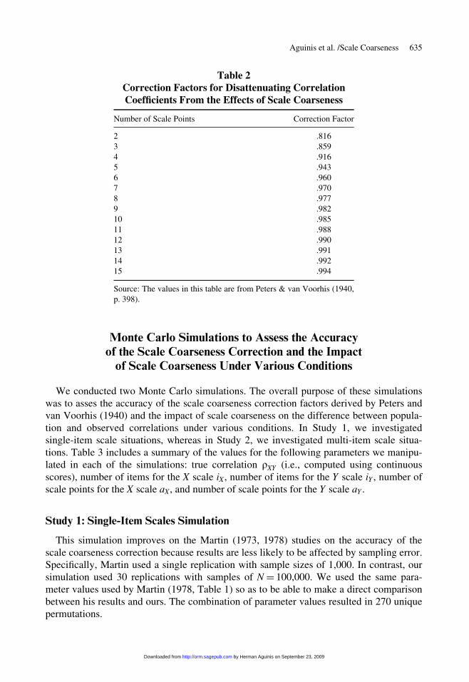
The correction assumes that the scaling intervals are centered around the midpoint of

the interval and is based on the following equation:

rx0y0 = rxy

rxx0ryy0ð1Þ

where rx0y0 is the disattenuated correlation, rxy is the observed correlation, and rxx0 and ryy0

are the correction factors for the number of scaling intervals on the X and Y scale, respec-

tively. Peters and van Voorhis (1940) also made assumptions about the underlying distri-

butions of X and Y and derived correction factors for normal and uniform distributions.

Table 2 includes the correction factors for a normal distribution.

As an example, if X includes 4 scale points (i.e., correction factor of .916; see Table 2)

and Y includes 5 scale points (i.e., correction factor of .943; see Table 2), disattenuating

an observed correlation of .35 using Equation 1 leads to:

rx0y0 = :35

ð:916Þð:943Þ = :41 ð2Þ

which represents an increase of about 17% in the magnitude of the correlation.




Monte Carlo Simulations to Assess the Accuracy

of the Scale Coarseness Correction and the Impact

of Scale Coarseness Under Various Conditions

We conducted two Monte Carlo simulations. The overall purpose of these simulations

was to asses the accuracy of the scale coarseness correction factors derived by Peters and

van Voorhis (1940) and the impact of scale coarseness on the difference between popula-

tion and observed correlations under various conditions. In Study 1, we investigated

single-item scale situations, whereas in Study 2, we investigated multi-item scale situa-

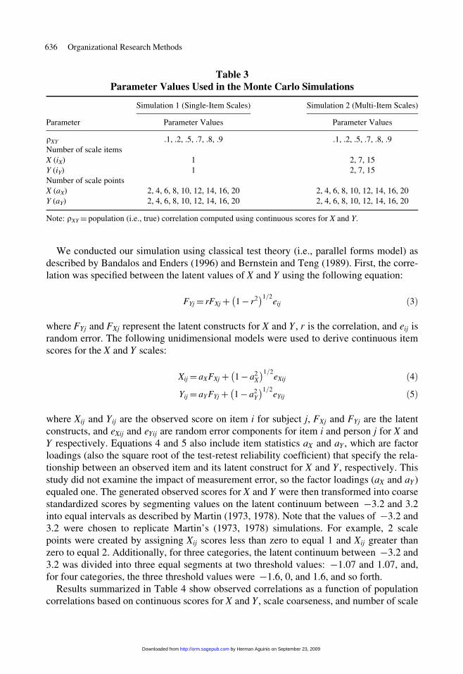
tions. Table 3 includes a summary of the values for the following parameters we manipu-

lated in each of the simulations: true correlation rXY (i.e., computed using continuous

scores), number of items for the X scale iX, number of items for the Y scale iY , number of

scale points for the X scale aX, and number of scale points for the Y scale aY .

Study 1: Single-Item Scales Simulation

This simulation improves on the Martin (1973, 1978) studies on the accuracy of the

scale coarseness correction because results are less likely to be affected by sampling error.

Specifically, Martin used a single replication with sample sizes of 1,000. In contrast, our

simulation used 30 replications with samples of N = 100,000. We used the same para-

meter values used by Martin (1978, Table 1) so as to be able to make a direct comparison

between his results and ours. The combination of parameter values resulted in 270 unique

permutations.

Table 2Correction Factors for Disattenuating CorrelationCoefficients From the Effects of Scale Coarseness

Number of Scale Points Correction Factor

2 .816

3 .859

4 .916

5 .943

6 .960

7 .970

8 .977

9 .982

10 .985

11 .988

12 .990

13 .991

14 .992

15 .994

Source: The values in this table are from Peters & van Voorhis (1940,

p. 398).




We conducted our simulation using classical test theory (i.e., parallel forms model) as

described by Bandalos and Enders (1996) and Bernstein and Teng (1989). First, the corre-

lation was specified between the latent values of X and Y using the following equation:

FYj = rFXj + 1− r2� �1=2

eij ð3Þ

where FYj and FXj represent the latent constructs for X and Y, r is the correlation, and eij is

random error. The following unidimensional models were used to derive continuous item

scores for the X and Y scales:

Xij = aXFXj + 1− a2X

� �1=2eXij ð4Þ

Yij = aY FYj + 1− a2Y

� �1=2eYij ð5Þ

where Xij and Yij are the observed score on item i for subject j, FXj and FYj are the latent

constructs, and eXij and eYij are random error components for item i and person j for X and

Y respectively. Equations 4 and 5 also include item statistics aX and aY , which are factor

loadings (also the square root of the test-retest reliability coefficient) that specify the rela-

tionship between an observed item and its latent construct for X and Y, respectively. This

study did not examine the impact of measurement error, so the factor loadings (aX and aY)

equaled one. The generated observed scores for X and Y were then transformed into coarse

standardized scores by segmenting values on the latent continuum between −3.2 and 3.2

into equal intervals as described by Martin (1973, 1978). Note that the values of −3.2 and

3.2 were chosen to replicate Martin’s (1973, 1978) simulations. For example, 2 scale

points were created by assigning Xij scores less than zero to equal 1 and Xij greater than

zero to equal 2. Additionally, for three categories, the latent continuum between −3.2 and

3.2 was divided into three equal segments at two threshold values: −1.07 and 1.07, and,

for four categories, the three threshold values were −1.6, 0, and 1.6, and so forth.

Results summarized in Table 4 show observed correlations as a function of population

correlations based on continuous scores for X and Y, scale coarseness, and number of scale

Table 3Parameter Values Used in the Monte Carlo Simulations

Simulation 1 (Single-Item Scales) Simulation 2 (Multi-Item Scales)

Parameter Parameter Values Parameter Values

rXY .1, .2, .5, .7, .8, .9 .1, .2, .5, .7, .8, .9

Number of scale items

X (iX) 1 2, 7, 15

Y (iY) 1 2, 7, 15

Number of scale points

X (aX) 2, 4, 6, 8, 10, 12, 14, 16, 20 2, 4, 6, 8, 10, 12, 14, 16, 20

Y (aY) 2, 4, 6, 8, 10, 12, 14, 16, 20 2, 4, 6, 8, 10, 12, 14, 16, 20

Note: rXY= population (i.e., true) correlation computed using continuous scores for X and Y.




points for X and Y. Recall that, similar to Martin (1973, 1978), this simulation included

one item for X and one item for Y and there was no measurement error. In Table 4, the col-

umn labeled M refers to observed correlations reported by Martin (1978, Table 1) and the

column labeled NS refers to observed correlations obtained in our new simulation. The

column labeled PvV shows attenuated correlations (by scale coarseness) that we computed

using Peters and van Voorhis (1940) correction factors. Specifically, we used Equation 1

to solve for the observed correlation rxy given that the population correlation is a known

parameter in our simulation.

Results shown in Table 4 indicate that, across all cells in the simulation design, differ-

ences between our generated correlations and those produced by the Peters and van Voor-

his (1940) correction procedure are negligible. Specifically, across all cells in our

simulation, the mean absolute-value difference between the correlations is .008, which

represents a coefficient of determination r2 = :000064. These results confirm Martin’s

conclusion regarding the accuracy of the Peters and van Voorhis (1940) correction factors.

Table 4 also shows that differences between our results and those obtained by Martin

(1978) are also negligible, given that the mean absolute-value difference between the cor-

relations is .01 (i.e., r2 = :001). As noted earlier, this negligible difference is due to the

use of more stable estimates in our simulation compared to Martin’s. Finally, Table 4 also

shows that differences between our correlations and those produced by the Peters and van

Voorhis correction factors, although still negligible, increase for correlation values of .7

or greater. This is an expected result because the correction factors are less precise for

‘‘extremely high correlations’’ (Peters & van Voorhis, 1940, p. 396). In any case, although

discrepancies are negligible and not practically significant in most situations, such extre-

mely large correlations are rare in the organizational sciences.

Table 4 also provides information regarding the conditions under which scale coarse-

ness produces the largest amount of bias. Specifically, as the number of scale points

decreases and the value of the population correlation increases, the effect of scale coarse-

ness becomes more pronounced. For example, an examination of the NS columns in Table

4 shows that a population correlation of .1 yields an observed correlation of .09 when Xand Y include 6 scale points each. However, the same population correlation is decreased

to a smaller value of .081 when X and Y include 4 scale points each. Considering the case

of a population correlation of .5, for 6 scale points for both X and Y the observed correla-

tion is .45 and this same population correlation is decreased substantially to .406 when 4

scale points are used.

Study 2: Multi-Item Scales Simulation

The second Monte Carlo simulation involved the use of multi-item scales for both Xand Y. There are several areas in the organizational sciences in which the use of single-

item scales is common (e.g., performance measurement and performance management,

Aguinis, 2009; job and life satisfaction, Judge et al., 2002). However, using multi-item

scales is typically advantageous because, compared to single-item scales, they are less

likely to suffer from deficiency and contamination and, therefore, they are superior in

terms of construct validity. In addition, multi-item scales are beneficial because they allow

for the computation of a greater variety of reliability estimates (e.g., internal consistency).




Tab

le4

Ob

serv

edC

orr

elati

on

Coef

fici

ents

as

aF

un

ctio

nof

Sca

leC

oars

enes

sR

eport

edb

yM

art

in(1

978),

Com

pu

ted

inth

eP

rese

nt

Stu

dy,

an

dC

om

pu

ted

Base

don

the

Corr

ecti

on

Fact

ors

Der

ived

by

Pet

ers

an

dvan

Voorh

is(1

940)

Corr

elat

ion

Bas

edon

Conti

nuous

Sca

les

for

Xan

dY

.1.2

.5.7

.8.9

Num

ber

of

Sca

leP

oin

ts

(X-Y

)M

NS

PvV

MN

SP

vV

MN

SP

vV

MN

SP

vV

MN

SP

vV

MN

SP

vV

20-2

0.0

94

.096

.099

.208

.195

.198

.505

.485

.496

.701

.681

.694

.803

.778

.793

.897

.875

.892

20-1

6.0

90

.098

.099

.209

.194

.198

.494

.485

.495

.701

.680

.692

.800

.777

.791

.891

.874

.890

20-1

4.0

90

.097

.099

.211

.194

.197

.499

.485

.494

.706

.679

.691

.800

.775

.790

.892

.873

.888

20-1

2.0

90

.097

.098

.201

.193

.197

.502

.484

.492

.702

.677

.689

.795

.774

.787

.886

.871

.886

20-1

0.0

88

.097

.098

.205

.193

.196

.494

.481

.490

.691

.674

.685

.781

.771

.783

.884

.867

.881

20-8

.103

.096

.097

.191

.191

.194

.491

.478

.485

.683

.668

.679

.785

.764

.776

.879

.860

.873

20-6

.103

.094

.095

.199

.188

.190

.478

.469

.476

.663

.657

.666

.767

.750

.761

.858

.844

.856

20-4

.095

.089

.090

.178

.179

.181

.462

.446

.451

.629

.624

.632

.735

.714

.722

.819

.803

.813

20-2

.078

.079

.081

.159

.160

.163

.401

.397

.407

.549

.557

.569

.638

.636

.650

.719

.716

.732

16-1

6.0

95

.096

.099

.207

.194

.197

.486

.485

.493

.689

.678

.691

.785

.775

.789

.888

.872

.888

16-1

4.0

95

.096

.098

.210

.194

.197

.484

.483

.492

.691

.677

.689

.792

.774

.788

.887

.871

.886

16-1

2.0

99

.097

.098

.201

.193

.196

.496

.482

.491

.684

.675

.687

.791

.772

.785

.885

.869

.884

16-1

0.0

97

.096

.098

.204

.192

.195

.484

.480

.488

.684

.672

.684

.786

.768

.781

.880

.865

.879

16-8

.103

.096

.097

.208

.190

.194

.487

.476

.484

.686

.667

.677

.775

.763

.774

.887

.858

.871

16-6

.108

.093

.095

.185

.188

.190

.485

.467

.474

.671

.655

.664

.762

.749

.759

.856

.842

.854

16-4

.094

.089

.090

.183

.178

.180

.450

.445

.450

.633

.623

.631

.727

.711

.721

.817

.801

.811

16-2

.072

.079

.081

.162

.159

.162

.390

.396

.406

.561

.555

.568

.638

.635

.649

.716

.714

.730

14-1

4.0

96

.096

.098

.213

.193

.197

.488

.483

.491

.694

.676

.688

.795

.772

.786

.887

.869

.885

14-1

2.0

99

.096

.098

.201

.192

.196

.505

.482

.490

.687

.674

.686

.788

.770

.784

.886

.867

.882

14-1

0.0

98

.096

.097

.210

.192

.195

.495

.479

.487

.681

.672

.682

.786

.767

.780

.880

.863

.877

14-8

.100

.095

.097

.205

.190

.193

.487

.475

.483

.682

.666

.676

.777

.760

.773

.877

.856

.869

14-6

.108

.093

.095

.187

.186

.189

.485

.467

.474

.670

.653

.663

.763

.747

.758

.856

.841

.852

14-4

.095

.088

.090

.182

.177

.180

.450

.445

.450

.633

.622

.629

.730

.711

.719

.819

.800

.809

14-2

.073

.080

.081

.162

.158

.162

.392

.395

.405

.563

.554

.567

.639

.634

.648

.717

.713

.728

12-1

2.1

10

.096

.098

.201

.192

.195

.492

.480

.488

.688

.672

.684

.784

.768

.781

.880

.864

.879

(Conti

nued

)

638



Tab

le4

(Con

tin

ued

)

Corr

elat

ion

Bas

edon

Conti

nuous

Sca

les

for

Xan

dY

.1.2

.5.7

.8.9

Num

ber

of

Sca

leP

oin

ts

(X-Y

)M

NS

PvV

MN

SP

vV

MN

SP

vV

MN

SP

vV

MN

SP

vV

MN

SP

vV

12-1

0.1

05

.095

.097

.181

.191

.194

.495

.478

.486

.681

.668

.680

.779

.765

.777

.875

.861

.875

12-8

.095

.094

.096

.205

.189

.193

.485

.475

.481

.677

.663

.674

.771

.758

.770

.871

.853

.866

12-6

.093

.093

.094

.198

.186

.189

.474

.465

.472

.663

.651

.661

.755

.745

.755

.853

.838

.850

12-4

.098

.089

.090

.189

.177

.179

.477

.443

.448

.635

.619

.627

.717

.708

.717

.815

.798

.807

12-2

.078

.079

.081

.155

.158

.161

.397

.395

.403

.554

.553

.565

.630

.631

.646

.712

.711

.726

10-1

0.0

92

.095

.097

.213

.190

.193

.485

.475

.483

.670

.666

.677

.777

.760

.773

.873

.856

.870

10-8

.090

.094

.096

.176

.189

.192

.479

.470

.479

.668

.660

.671

.768

.755

.766

.868

.849

.862

10-6

.086

.092

.094

.180

.185

.188

.471

.463

.470

.659

.649

.658

.758

.741

.751

.848

.834

.845

10-4

.098

.088

.089

.171

.176

.178

.455

.442

.446

.632

.617

.624

.720

.705

.713

.811

.793

.803

10-2

.072

.078

.080

.160

.157

.161

.397

.394

.401

.549

.550

.562

.633

.629

.642

.711

.708

.723

8-8

.095

.093

.095

.201

.188

.190

.479

.468

.475

.675

.654

.664

.768

.748

.759

.862

.841

.854

8-6

.091

.091

.093

.182

.183

.186

.474

.459

.465

.653

.642

.651

.750

.734

.745

.843

.826

.838

8-4

.088

.086

.088

.171

.175

.177

.446

.437

.442

.625

.611

.618

.710

.699

.707

.808

.786

.795

8-2

.078

.078

.080

.160

.155

.159

.391

.389

.398

.550

.545

.557

.626

.623

.636

.710

.701

.716

6-6

.095

.090

.091

.183

.180

.183

.455

.450

.456

.640

.630

.639

.738

.720

.730

.828

.812

.821

6-4

.079

.085

.087

.178

.172

.173

.432

.429

.433

.614

.600

.606

.695

.685

.693

.790

.772

.780

6-2

.076

.076

.078

.151

.152

.156

.383

.381

.390

.534

.535

.546

.612

.611

.624

.692

.690

.702

4-4

.081

.081

.082

.164

.163

.164

.413

.406

.411

.587

.570

.576

.664

.655

.658

.770

.755

.740

4-2

.071

.072

.074

.144

.144

.148

.364

.363

.370

.517

.511

.518

.588

.589

.592

.680

.680

.666

2-2

.064

.064

.067

.126

.128

.133

.331

.333

.333

.491

.494

.467

.590

.591

.533

.711

.713

.600

Note

:M

=re

port

edby

Mar

tin

(1978);

NS=

resu

lts

obta

ined

inth

enew

sim

ula

tion

conduct

edas

par

tof

the

pre

sent

study;

PvV=

com

pute

dusi

ng

corr

ecti

on

fac-

tors

der

ived

by

Pet

ers

and

van

Voorh

is(1

940).

639



Thus, because multi-item scales are usually beneficial regarding both conceptual and sta-

tistical issues, the majority of research domains in the organizational sciences favor their

use over single-item scales.

Accordingly, in Study 2 we generated multiple items via a unidimensional parallel

forms classical test theory model (i.e., equal item locations and factor loadings across

items) using the approach outlined by Bandalos and Enders (1996) described earlier. That

is, a normally distributed latent variable was generated for each subject. A key difference

from Study 1 is that we generated continuous items i by specifying the relationship

between each item and the latent variable (the factor loadings were held constant across

items to one, so there was no measurement error). Coarse items were then created using

equal intervals as described earlier for single-item scales and total scores were computed.

The coarse items were them summed to create total scores for X and Y and the observed

correlation was computed between the two coarse scales. The parameter values used are

summarized in Table 3 and combining these values resulted in a total of 2,268 unique

permutations.

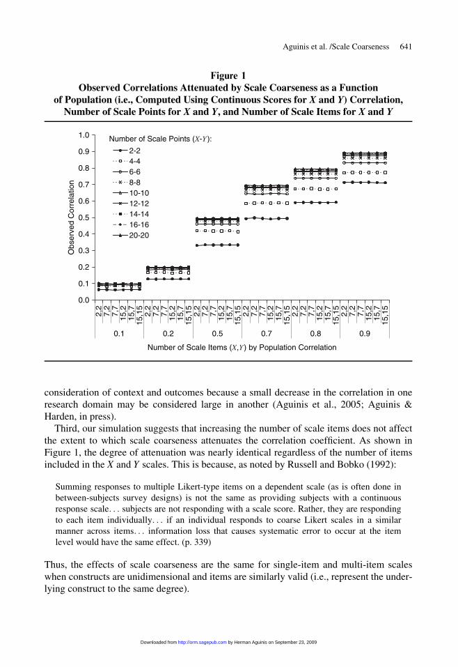
Results of Study 2 are displayed in Figure 1. As shown in this figure, increasing the

number of items for the X and Y scales did not affect the impact of scale coarseness on the

observed correlations. We computed standard deviations of the observed correlations

within each number-of-items condition. Of the 2,268 unique permutations in the simula-

tion, there were 486 unique combinations of scale points. We computed the observed cor-

relations for each of these 486 cells and the standard deviation for the correlations to

assess any variability due to number of scale items. The average of these 486 standard

deviations was 0.0009, which indicates negligible fluctuations in the observed correlations

for different numbers of items within each combination of scale points.

Summary and Conclusions

Results from Study 1 and Study 2, together with results reported by Martin (1973,

1978) about the accuracy of the correction factors and the conditions under which scale

coarseness affects observed correlations, lead to the following conclusions. First, in terms

of accuracy, the Peters and van Voorhis (1940) correction factors are accurate across the

entire range of possible values for the correlation coefficient. The correction factors are

not as accurate for correlations of about .7 or larger, but the amount of discrepancy is neg-

ligible in most situations (i.e., around .01 on average). Also, these correction factors are

accurate for item scale points ranging from 2 to 20. This conclusion supports findings by

Martin (1973, 1978), but our conclusion is based on more stable and precise estimates of

the degree of attenuation produced by scale coarseness, given our sample size of 100,000

and the use of 30 replications per design condition. In contrast, Martin simulated sample

sizes of 1,000 and did not use replications.

Second, the effect of scale coarseness is more pronounced for situations involving

fewer scale points and larger correlations. In terms of scale points, using scales with 8 or

fewer scale points is likely to produce noticeable decreases in the observed correlation. In

addition, this decrease is more noticeable for correlations that are about .30 or larger. We

emphasize that these are general rules of thumb that may not be meaningful without a




consideration of context and outcomes because a small decrease in the correlation in one

research domain may be considered large in another (Aguinis et al., 2005; Aguinis &

Harden, in press).

Third, our simulation suggests that increasing the number of scale items does not affect

the extent to which scale coarseness attenuates the correlation coefficient. As shown in

Figure 1, the degree of attenuation was nearly identical regardless of the number of items

included in the X and Y scales. This is because, as noted by Russell and Bobko (1992):

Summing responses to multiple Likert-type items on a dependent scale (as is often done in

between-subjects survey designs) is not the same as providing subjects with a continuous

response scale. . . subjects are not responding with a scale score. Rather, they are responding

to each item individually. . . if an individual responds to coarse Likert scales in a similar

manner across items. . . information loss that causes systematic error to occur at the item

level would have the same effect. (p. 339)

Thus, the effects of scale coarseness are the same for single-item and multi-item scales

when constructs are unidimensional and items are similarly valid (i.e., represent the under-

lying construct to the same degree).

Figure 1

Observed Correlations Attenuated by Scale Coarseness as a Functionof Population (i.e., Computed Using Continuous Scores for X and Y) Correlation,

Number of Scale Points for X and Y, and Number of Scale Items for X and Y

0.0

0.1

0.2

0.3

0.4

0.5

0.6

0.7

0.8

0.9

1.0

2,2

7,2

7,7

15,2

15,7

15,1

52,

27,

27,

715

,215

,715

,15

2,2

7,2

7,7

15,2

15,7

15,1

52,

27,

27,

715

,215

,715

,15

2,2

7,2

7,7

15,2

15,7

15,1

52,

27,

27,

715

,215

,715

,15

0.1 0.2 0.5 0.7 0.8 0.9

Number of Scale Items (X,Y) by Population Correlation

Obs

erve

d C

orre

latio

n

2-24-46-68-810-1012-1214-1416-1620-20

Number of Scale Points (X-Y ):




Sampling Error and Confidence Interval Computations

for the Corrected Correlation

As is the case for the effects of other methodological artifacts, correcting for scale coarse-

ness results in a sampling error that is larger than the sampling error of the uncorrected

correlation (cf. Bobko, 1983; Bobko & Rieck, 1980). Consequently, confidence intervals

around the corrected correlation are also wider than those around the observed correlations.

Peters and van Voorhis (1940) did not provide equations for computing sampling error var-

iance or confidence intervals for the corrected correlation and, to the best of our knowledge,

these equations are not available elsewhere. Bobko and Rieck (1980) and Hunter and

Schmidt (2004, pp. 118-120) provided an equation for the sampling error variance for the

correlation coefficient corrected for simple artifacts such as measurement error and artificial

dichotomization of continuous variables. This equation is the following:

s2ec= s2

e

A2ð6Þ

where A is the correction factor and s2e , the sampling error for the observed (i.e., uncor-

rected) correlation, is

s2e =ð1− r2

xyÞ2

N − 1ð7Þ

Next, we replace A in Equation 6 with the correction factor for scale coarseness to

obtain the sampling error variance for the correlation coefficient in an individual study

corrected for scale coarseness:

s2ec= s2

e

ðrxx0ryy0 Þ2ð8Þ

where rxx0 and ryy0 are the correction factors for scale coarseness on the predictor and the

criterion as defined in Equation 1. To compute a confidence interval for the corrected cor-

relation, we apply the correction shown in Equation 1 to the lower and upper limits of the

interval.

For example, consider a study in which the observed correlation is .20, X is overall job

satisfaction measured using a 5-point scale (e.g., Fuller et al., 2003) and Y is job performance

measured using a 3-point scale (e.g., Lyness & Heilman, 2006). Using Equation 1 yields:

rx0y0 = :20

ð:943Þð:859Þ = :25 ð9Þ

Thus, in this realistic example based on articles published recently, scale coarseness

reduced the correlation by 20%. To compute a confidence interval around the corrected

correlation, we must first obtain the sampling error for the observed (i.e., uncorrected) cor-

relation using Equation 7. Assuming that sample size in this study is 100,




s2e =ð1− :202Þ2

100− 1= :0093 ð10Þ

And, using Equation 8, the sampling error in the corrected correlation is

s2ec= s2

e

ðrxx0ryy0 Þ2= :0093

ð½:943�½:859�Þ2= :0142 ð11Þ

The 95% confidence interval for the observed correlation is rxy ± 1:96se, which is

:01≤ rxy ≤ :39. Correcting the lower limit yields :01ð:943Þð:859Þ = :01 and correcting the upper

limit yields :39ð:943Þð:859Þ = :48. This results in a 95% confidence interval for the corrected

correlation of :01≤ rx0y0≤ :48. Thus, the center of the confidence interval shifts from the

observed correlation of .20 to the corrected correlation of .25. Also, the width of the confi-

dence interval around the corrected value is about 24% larger than the width of the confi-

dence interval around the observed value, demonstrating that sampling error is larger in

the corrected correlation.

Online Computational Tool for Correcting Individual Correlations

Blanton and Jaccard (2006) noted that the use of coarse scales is typical yet problematic

in psychology research. In addition, as confirmed by our Web of Science literature search

noted previously, researchers in the organizational sciences are not aware of the procedure

to correct the correlation coefficient for the bias caused by scale coarseness. Even if a

researcher is aware that scale coarseness is an important methodological artifact, he or she

may not implement a correction because of a lack of a computational tool that allows for

its implementation. This may be another reason why the correction has been implemented

in only one of the more than 15,000 articles published in organizational science journals

since the publication of Peters and van Voorhis’s book in 1940. Finally, neither Peters and

van Voorhis’s book nor any other published source of which we are aware provides equa-

tions to compute the sampling error or confidence intervals for the corrected correlation.

Accordingly, we developed a user-friendly computer program that allows researchers to cor-

rect correlation coefficients for scale coarseness. The program is available free of charge

and can be executed online by visiting the following Web site: http://carbon.cudenver.edu/

∼haguinis/ (please click on the ‘‘Scale Coarseness Program’’ link).

As an illustration, Figure 2 includes a screen shot of the program. Users input the

observed correlation and number of scale points for each of the two variables. In the

hypothetical yet realistic example shown in Figure 2, the observed correlation is .35 and

each of the two variables were measured using 5-point scales. Figure 2 shows a disattenu-

ated correlation of about .39, which represents an increase of about 13% in the correlation’s

magnitude. In addition to the observed correlation and number of scale points for the predic-

tor and criterion, the program includes an input box for sample size (N). This information is

needed so the program can compute the sampling error as well as confidence intervals for

the corrected correlation using the equations described previously. In this particular example




shown in Figure 2, the sampling error variance for the observed correlation is .0078 and the

sampling error variance for the corrected correlation is .0098 (i.e., an increase of approxi-

mately 25%). In addition, the screen shot displayed in Figure 2 shows that the 95% confi-

dence interval for the observed correlation of .35 ranges from .18 to .52, whereas the 95%

confidence interval for the corrected correlation of .39 ranges from .20 to .59. For the sake

of completeness, the program’s output also includes 90% and 99% confidence intervals for

both the observed and corrected correlation. Next, we describe a new procedure that allows

researchers to incorporate the scale coarseness correction in a meta-analysis.

Incorporating the Scale Coarseness Correction in a Meta-Analysis

Thus far, our discussion has focused on the scale coarseness correction of a correlation

coefficient in an individual study (i.e., primary-level studies). However, a meta-analyst

Figure 2

Screen Shot of Computer Program That Implements All Computationsfor (a) Correcting Correlations Attenuated From Using Coarse Scales,

and (b) Calculating Sampling Error and Confidence Intervalsfor the Observed as well as Corrected Correlations

Note: The program is available at http://carbon.cudenver.edu/∼haguinis (please click on the ‘‘Scale Coarseness Program’’

link).




may wish to correct the observed correlations as reported in primary-level studies and then

meta-analyze the resulting corrected correlations. Moreover, a meta-analyst may wish to

correct for the effects of scale coarseness and also for the bias introduced by other metho-

dological artifacts (e.g., measurement error in X and/or Y, dichotomization of a truly con-

tinuous variable, direct range restriction). Despite this need, the scale coarseness artifact is

not discussed in any of the most widely cited and used sources on meta-analytic methods

(e.g., Hedges & Olkin, 1985; Hunter & Schmidt, 2004) or in any of the articles published

in the ORM feature topic on meta-analysis in January 2008 (Aguinis et al., 2008; Bobko

& Roth, 2008; Dalton & Dalton, 2008; Kisamore & Brannick, 2008; Schmidt, 2008; Steel

& Kammeyer-Mueller, 2008; Wood, 2008). Also, we are not aware of any published

source describing an extension of the scale coarseness correction from the primary to the

meta-analytic level.

Correcting correlations for scale coarseness at the meta-analytic level is feasible in orga-

nizational science research because scale coarseness information is usually available for

each of the studies included in a meta-analysis. In other words, the Method section of each

article included in a meta-analytic review is likely to include information about the mea-

sures and number of items and scale points used. The availability of this information repre-

sents an advantage in comparison to other artifacts for which a correction factor may not be

available at the individual study level or at all (e.g., range restriction, Halbesleben, 2006).

Hunter and Schmidt (2004, chapter 3) provide a description of how to apply corrections

based on several methodological artifacts simultaneously. Hunter and Schmidt’s equations

provide a framework for incorporating a scale coarseness correction factor in a meta-

analysis. Essentially, one computes a compound multiplicative attenuation factor including

all of the correctable artifacts for each study included in the meta-analysis. For example, if

a1 is the attenuation factor for reliability of the predictor X (i.e.,ffiffiffiffiffiffirxxp

) and a2 is the attenua-

tion factor for reliability of the criterion Y (i.e.,ffiffiffiffiffiryyp

), the compound attenuation factor for

these two artifacts is A= a1a2. The value for each of these attenuation factors may be

known for each individual study. However, most likely this information is not available for

each study. Thus, the attenuation factor is an average of the study-level attenuation factor

information for those studies for which this information is available (Hunter & Schmidt,

2004, chapter 4).

Note that the order of the corrections only matters in the presence of the range restriction

correction. This is because all artifacts, including scale coarseness, are simple artifacts except

for range restriction. We could not think of any reason nor did we find a reason in the litera-

ture for why scale coarseness should not be considered an additional simple artifact.

Hunter et al. (2006) reached the following conclusion regarding situations when there is

no range restriction: ‘‘If several simple artifacts are present in a study, their effects com-

bine in a simple multiplicative way. The order in which the artifacts are entered does not

play a role. The final result is the same for any order’’ (p. 595). When range restriction is

present and corrected for, then it is important to understand at which point in the research

process direct and/or indirect range restriction had an effect because this will determine

when the range restriction correction will be applied in a meta-analysis. For instance, in

many human resource–management research domains, including staffing and performance

management, the criterion typically used is supervisory ratings (Aguinis, 2009). But per-

formance scores of job incumbents suffer from direct range restriction in relationship to




performance scores that would be obtained from job applicants. In this case, the direct

range restriction correction should be applied before the correction for measurement error,

scale coarseness, and other simple artifacts. This is because the measurement errors in the

performance scores and the coarseness in the performance scale are not affected by and

appear after the distribution is already range restricted (i.e., by virtue of including job

incumbents only). Alternatively, in the case of indirect range restriction, the range restric-

tion correction is applied after the measurement error and scale coarseness corrections.

We refer readers to Hunter et al.’s (2006) detailed discussion of the issue of the ordering

of corrections in meta-analysis.

We can incorporate the scale coarseness correction by adding the scale coarseness

attenuation factor asc = rxx0ryy0 , as defined in Equation 1, resulting in a compound attenua-

tion factor A= a1a2asc. Thus, the corrected correlation is rx0y0 = rxy

A . To compute the sam-

pling error variance for the corrected correlation, we first obtain the sample-size weighted

mean observed correlation �rxy and compute the sampling error variance for the observed

correlation as follows (Aguinis, 2001):

s2rxy

= ð1− �r2xyÞ

2

N − 1ð12Þ

where N is the sample size for the study under consideration. Note that using �rxy instead of

rxy yields a more accurate sampling error estimate for the uncorrected correlation (Agui-

nis, 2001). Similar to Equation 6 and following Hunter and Schmidt (2004, pp. 118-120),

the sampling error variance for the corrected correlation is:

s2rx0y0

= s2rxy

A2ð13Þ

Finally, we acknowledge that the possibility that researchers may overcorrect correlations

is a long-standing and unresolved issue in the meta-analysis literature (e.g., James, Demaree,

& Mulaik, 1986; James, Demaree, Mulaik, & Mumford, 1988). Thus, future research could

investigate potential concurrent effects of scale coarseness, various types of measurement

error, and other artifacts such as direct and indirect range restriction. There are several ques-

tions that this simulation could address, such as the extent to which scale coarseness may

interact with some but not other sources of measurement error in biasing the correlation

coefficient. Thus, future simulations could manipulate various types of measurement error

(e.g., because of items, raters, time, or a combination; Schmidt, Le, & Ilies, 2003) and range

restriction (direct, indirect; Hunter et al., 2006), in combination with scale coarseness. This

would be a large-scale simulation that goes beyond the scope of the present article.

Conclusion

Because of the pervasive use of Likert-type scales to measure continuous constructs in

organizational science research, scale coarseness is a common methodological artifact that

causes a downward bias in the correlation coefficient in many situations. As noted by




Russell and Bobko (1992) within the specific context of estimating moderating effects,

but equally valid for the estimation of the correlation coefficient, ‘‘Investigators should

not attempt to discover moderator effects unless the overt measurement scale contains at

least as many response options as exist in the theoretical response domain’’ (p. 339).

Although seldom acknowledged and seemingly unbeknownst to most organizational

science researchers, the operationalization of continuous constructs using Likert-type

scales attenuates correlation coefficients systematically in many situations. In addition to

being a pervasive phenomenon in virtually all areas of organizational science research,

this downward bias can be meaningful, be nontrivial, and lead to substantive changes in

theory and practice (e.g., in staffing decision making), particularly in situations with few

scale points and large absolute values for the correlation coefficient. In many cases, the

magnitude of the downward bias is comparable to that caused by measurement error and

range restriction, which are the two methodological artifacts most frequently studied in

the organizational sciences besides sampling error.

Given the availability of the computer program described in this article, future primary-

level studies assessing continuous constructs, particularly those relying on the use of mea-

sures with few scale points, should report correlations disattenuated from the effects of scale

coarseness as well as confidence intervals for the corrected correlations. We also recommend

that future meta-analytic reviews incorporate the scale coarseness correction described in this

article. Considering that the information needed to correct correlations for scale coarseness is

likely to be available in most studies included in a meta-analysis, we suggest that scale coar-

seness be added to the list of correctable methodological artifacts (cf. Hunter & Schmidt,

2004, Table 3.1, p. 76). The scale coarseness correction could be applied routinely as is done

with other commonly corrected artifacts such as measurement error and range restriction. As

noted by Schmidt et al. (2006), ‘‘Because of its implications for theory development, accu-

racy of estimation of important parameters is critical in any science’’ (p. 281). Applying the

scale coarseness correction at the primary and meta-analytic levels will lead to more accurate

estimates of construct-level correlation coefficients.

Notes

1. A concern with the use of these types of scales is that they do not have interval-level properties (cf.

Aguinis, Henle, & Ostroff, 2001). Specifically, the concern is that the resulting data are only ordinal and using

a maximum likelihood (ML) factor analysis may result in biased parameter estimates. The polychoric correla-

tion, proposed by Ritchie-Scott (1918) and perfected by Pearson and Pearson (1922), has resurfaced in the lit-

erature as a way to conduct a ML factor analysis using data collected with ordinal-level scales (e.g., Flora,

Finkel, & Foshee, 2003; Holgado Tello, Chacon Moscoso, Barbero Garcia, & Sanduvete Chaves, 2006). The

polychoric correlation is a correlation that would be obtained if the ordinal-level distributions were actually

interval-level (the polyserial correlation is used when one of the scales is ordinal and the other is continuous).

In these ML factor analyses based on ordinal data, there is a need to first estimate a matrix of polychoric corre-

lations and then compute a weight matrix (i.e., the inverse of the asymptotic covariance matrix of polychoric

correlations). Although the computations are quite complex (Bedrick & Breslin, 1996; Lee & Poon, 1986;

Olsson, 1979; Poon & Lee, 1987), some commercially available software packages now allow users to com-

pute polychoric and/or polyserial correlations (e.g., SAS, R, PRELIS, MPlus).

In a nutshell, the computation of a polychoric correlation consists of adding tails to the distributions, and it

is therefore an estimate relying heavily on the assumption of an underlying continuous bivariate normal distribu-

tion. Unfortunately, this assumption is violated frequently and this violation has important consequences in terms




of the precision of the resulting estimate (Homer & O’Brien, 1988). A second limitation of using polychoric cor-

relations in conducting a ML factor analysis is that an accurate estimation of the weight matrix requires a large

sample size, and inaccurate estimates can be obtained with a sample size as large as 200 (Dolan, 1994). It is

encouraging that recent developments are attempting to overcome these and other challenges (e.g., Song & Lee,

2003; Zhang & Browne, 2006).

2. Although they are caused by different mechanisms, in some situations scale coarseness and artificial

dichotomization (or polychotomization) can produce the same outcome in terms of the resulting data structure.

For example, a researcher may artificially trichotomize a truly continuous variable after data have been col-

lected and assign values to individuals such that 1=Group 1, 2=Group 2, and 3=Group 3. In this situation,

the resulting data structure would be identical to the one produced by using a coarse 3-point scale as in the

example just discussed.

3. If the confidence interval around the uncorrected correlation includes the correlation corrected for scale

coarseness, then one cannot rule out the possibility that a value closer to the corrected estimate would be

obtained in a separate sample. This caveat regarding the scale coarseness correction in relation to sample size

is equally applicable to all other statistical and methodological corrections (e.g., measurement error, range

restriction).

References

Aguinis, H. (2001). Estimation of sampling variance of correlations in meta-analysis. Personnel Psychology,

54, 569-590.

Aguinis, H. (2009). Performance management (2nd ed.). Upper Saddle River, NJ: Pearson Prentice Hall.

Aguinis, H., Beaty, J. C., Boik, R. J., & Pierce, C. A. (2005). Effect size and power in assessing moderating

effects of categorical variables using multiple regression: A 30-year review. Journal of Applied Psychology,

90, 94-107.

Aguinis, H., Bommer, W. H., & Pierce, C. A. (1996). Improving the estimation of moderating effects by using

computer-administered questionnaires. Educational and Psychological Measurement, 56, 1043-1047.

Aguinis, H., & Harden, E. E. (in press). Sample size rules of thumb: Evaluating three common practices.

In C. E. Lance & R. J. Vandenberg (Eds.), Statistical and methodological myths and urban legends:

Received doctrine, verity, and fable in the organizational and social sciences. Mahwah, NJ: Lawrence

Erlbaum.

Aguinis, H., Henle, C. A., & Ostroff, C. (2001). Measurement in work and organizational psychology.

In N. Anderson, D.S. Ones, H. K. Sinangil, & C. Viswesvaran (Eds.), Handbook of industrial, work and

organizational psychology (Vol. 1, pp. 27-50). London: Sage.

Aguinis, H., & Pierce, C. A. (1998). Testing moderator variable hypotheses meta-analytically. Journal of

Management, 24, 577-592.

Aguinis, H., & Smith, M. A. (2007). Understanding the impact of test validity and bias on selection errors and

adverse impact in human resource selection. Personnel Psychology, 60, 165-199.

Aguinis, H., Sturman, M. C., & Pierce, C. A. (2008). Comparison of three meta-analytic procedures for esti-

mating moderating effects of categorical variables. Organizational Research Methods, 11, 9-34.

Aguinis, H., & Whitehead, R. (1997). Sampling variance in the correlation coefficient under indirect range

restriction: Implications for validity generalization. Journal of Applied Psychology, 82, 528-538.

Aiken, L. R. (1983). Number of response categories and statistics on a teacher rating scale. Educational and

Psychological Measurement, 43, 397-401.

Allen, T. D., Eby, L. T., & Lentz, E. (2006). The relationship between formal mentoring program characteris-

tics and perceived program effectiveness. Personnel Psychology, 59, 125-153.

Andrews, F. M., & Farris, G. F. (1972). Time pressure and performance of scientists and engineers: A 5-year

panel study. Organizational Behavior and Human Performance, 8, 185-200.

Arnold, H. J. (1981). A test of the multiplicative hypothesis of expectancy valence theories of work motiva-

tion. Academy of Management Journal, 24, 128-141.




Ash, P. (1971). Screening employment applicants for attitudes toward theft. Journal of Applied Psychology,

55, 161-164.

Bandalos, D. L., & Enders, C. K. (1996). The effects of nonnormality and number of response categories on

reliability. Applied Measurement in Education, 9, 151-160.

Barrick, M. R., Bradley, B. H., Kristof-Brown, A. L., & Colbert, A. E. (2007). The moderating role of top

management team interdependence: Implications for real teams and working groups. Academy of Manage-

ment Journal, 50, 544-557.

Bendig, A. W. (1953). The reliability of self-ratings as a function of the amount of verbal anchoring and the

number of categories on the scales. Journal of Applied Psychology, 37, 38-41.

Bendig, A. W. (1954). Reliability and the number of rating scale categories. Journal of Applied Psychology,

38, 38-40.

Bedrick, E. J., & Breslin, F. C. (1996). Estimating the polyserial correlation coefficient. Psychometrika, 61,

427-443.

Bernstein, I. H., & Teng, G. (1989). Factoring items and factoring scales are different: Spurious evidence for

multidimensionality due to item categorization. Psychological Bulletin, 105, 467-477.

Blanton, H., & Jaccard, J. (2006). Arbitrary metrics in Psychology. American Psychologist, 61, 27-41.

Bobko, P. (1983). An analysis of correlations corrected for attenuation and range restriction. Journal of

Applied Psychology, 68, 584-589.

Bobko, P., & Rieck, A. (1980). Large sample estimators for standard errors of functions of correlation coeffi-

cients. Applied Psychological Measurement, 4, 385-398.

Bobko, P., & Roth, P. L. (2008). Psychometric accuracy and (the continuing need for) quality thinking in

meta-analysis. Organizational Research Methods, 11, 114-126.

Bollen, K. A., & Barb, K. H. (1981). Pearson’s r and coarsely categorized measures. American Sociological

Review, 46, 232-239.

Bowling, N. A., & Beehr, T. A. (2006). Workplace harassment from the victim’s perspective: A theoretical

model and meta-analysis. Journal of Applied Psychology, 91, 998-1012.

Brown, D. J., Cober, R. T., Kane, K., Levy, P. E., & Shalhoop, J. (2006). Proactive personality and the success-

ful job search: A field investigation with college graduates. Journal of Applied Psychology, 91, 717-726.

Buel, W. D. (1965). Biographical data and the identification of creative research personnel. Journal of Applied

Psychology, 49, 318-321.

Buel, W. D. (1969). A reply to ‘‘personal data as a predictor of small finance company credit risk’’ by Moran,

Walsh, Clement, and Bumbeck. Personnel Psychology, 22, 57-60.

Carlson, R. E. (1967). Selection interview decisions: Relative influence of appearance and factual written

information on an interviewer’s final rating. Journal of Applied Psychology, 51, 461-468.

Carlson, R. E. (1969). Relative influence of a photograph vs. factual written information on an interviewer’s

employment decision. Personnel Psychology, 22, 45-56.

Cohen, J. (1983). The cost of dichotomization. Applied Psychological Measurement, 7, 249-253.

Cohen, J. (1988). Statistical power analysis for the behavioral sciences (2nd ed.). Hillsdale, NJ: Erlbaum.

Corrigan, P. W., Holmes, E. P., Luchins, D., Buican, B., Basit, A., & Parks, J. J. (1994). Staff burnout in a

psychiatric-hospital: A cross-lagged panel design. Journal of Organizational Behavior, 15, 65-74.

Cramton, C. D., Orvis, K. L., & Wilson, J. M. (2007). Situation invisibility and attribution in distributed colla-

borations. Journal of Management, 33, 525-546.

Dalton, D. R., & Dalton, C. M. (2008). Meta-analyses: Some very good steps toward a bit longer journey.

Organizational Research Methods, 11, 127-147.

Dierdorff, E. C., & Surface, E. A. (2007). Placing peer ratings in context: Systematic influences beyond ratee

performance. Personnel Psychology, 60, 93-126.

Dolan, C. V. (1994). Factor analysis of variables with 2, 3, 5, and 7 response categories: A comparison of cate-

gorical variable estimators using simulated data. British Journal of Mathematical and Statistical Psychology,

47, 309-326.

Edwards, J. R. (2001). Ten difference score myths. Organizational Research Methods, 4, 265-287.

Fedor, D. B., Caldwell, S., & Herold, D. M. (2006). The effects of organizational changes on employee

commitment: A multilevel investigation. Personnel Psychology, 59, 1-29.




Ferrin, D. L., Dirks, K. T., & Shah, P. P. (2006). Direct and indirect effects of third party relationships on

interpersonal trust. Journal of Applied Psychology, 91, 870-883.

Flora, D. B., Finkel, E. J., & Foshee, V. A. (2003). Higher order factor structure of a self-control test:

Evidence from confirmatory factor analysis with polychoric correlations. Educational and Psychological

Measurement, 63, 112-127.

Fong, E. A., & Tosi, H. L. (2007). Effort, performance, and conscientiousness: An agency theory perspective.

Journal of Management, 33, 161-179.

Fuller, J. A., Stanton, J. M., Fisher, G. G., Spitzmuller, C., Russell, S. S., & Smith, P. C. (2003). A lengthy

look at the daily grind: Time series analysis of events, mood, stress, and satisfaction. Journal of Applied

Psychology, 88, 1019-1033.

Garner, W. R. (1960). Rating scales, discriminability, and information transmission. Psychological Review,

67, 343-352.

George, J. M., & Zhou, J. (2007). Dual tuning in a supportive context: Joint contributions of positive mood,

negative mood, and supervisory behaviors to employee creativity. Academy of Management Journal, 50,

605-622.

Griffin, M. A., Neal, A., & Parker, S. K. (2007). A new model of work role performance: Positive behavior in

uncertain and interdependent contexts. Academy of Management Journal, 50, 327-347.

Gross, I. (1972). Creative aspects of advertising. Sloan Management Review, 14(1), 83-109.

Guilford, J. P. (1954). Psychometric methods (2nd ed.). New York: McGraw-Hill.

Halbesleben, J. R. B. (2006). Sources of social support and burnout: A meta-analytic test of the conservation

of resources model. Journal of Applied Psychology, 91, 1134-1145.

Hedges, L. V., & Olkin, I. (1985). Statistical methods for meta-analysis. Orlando, FL: Academic Press.

Heslin, P. A., Vandewalle, D., & Latham, G. P. (2006). Keen to help? Managers’ implicit person theories and

their subsequent employee coaching. Personnel Psychology, 59, 871-902.

Holgado Tello, F. P., Chacon Moscoso, S., Barbero Garcia, I., & Sanduvete Chaves, S. (2006). Training

satisfaction rating scale: Development of a measurement model using polychoric correlations. European

Journal of Psychological Assessment, 22, 268-279.

Homer, P., & O’Brien, R. M. (1988). Using LISREL models with crude rank category measures. Quality &

Quantity, 22, 191-201.

Hunter, J. E., & Schmidt, F. L. (2004). Methods of meta-analysis: Correcting error and bias in research find-

ings (2nd ed.). Thousand Oaks, CA: Sage.

Hunter, J. E., Schmidt, F. L. & Le, H. (2006). Implications of direct and indirect range restriction for meta-

analysis methods and findings. Journal of Applied Psychology, 91, 594-612.

James, L. R., Demaree, R. G., & Mulaik, S. A. (1986). A note on validity generalization procedures. Journal

of Applied Psychology, 71, 440-450.

James, L. R., Demaree, R. G., Mulaik, S. A., & Mumford, M. D. (1988). Validity generalization: Rejoinder to

Schmidt, Hunter, and Raju (1988). Journal of Applied Psychology, 73, 673-678.

Judge, T. A., Heller, D., & Mount, M. K. (2002). Five-factor model of personality and job satisfaction:

A meta-analysis. Journal of Applied Psychology, 87, 530-541.

Kemery, E. R., Dunlap, W. P., & Griffeth, R. W. (1988). Correction for variance restriction in point-biserial

correlations. Journal of Applied Psychology, 73, 688-691.

Kisamore, J. L., & Brannick, M. T. (2008). An illustration of the consequences of meta-analysis model choice.

Organizational Research Methods, 11, 35-53.

Klein, H. J., Noe, R. A., & Wang, C. (2007). Motivation to learn and course outcomes: The impact of delivery

mode, learning goal orientation, and perceived barriers and enablers. Personnel Psychology, 59, 665-702.

Komorita, S. S., & Graham, W. K. (1965). Number of scale-points and the reliability of scales. Educational

and Psychological Measurement, 25, 987-995.

Krieg, E. F. (1999). Biases induced by coarse measurement scales. Educational and Psychological Measure-

ment, 59, 749-766.

Lam, W., Huang, X., & Snape, E. (2007). Feedback-seeking behavior and leader-member exchange:

Do supervisor-attributed motives matter? Academy of Management Journal, 50, 348-363.




Le, H., Oh, I., Shaffer, J., & Schmidt, F. L. (2007). Implications of methodological advances for the practice of

personnel selection: How practitioners benefit from meta-analysis. Academy of Management Perspectives,

21(3), 6-15.

Lee, S., & Poon, W. (1986). Maximum likelihood estimation of polyserial correlations. Psychometrika, 51,

113-121.

Lyness, K. S., & Heilman, M. E. (2006). When fit is fundamental: Performance evaluations and promotions of

upper-level female and male managers. Journal of Applied Psychology, 91, 777-785.

Marcus, B., Lee, K., & Ashton, M. C. (2007). Personality dimensions explaining relationships between integrity

tests and counterproductive behavior: Big Five, or one in addition? Personnel Psychology, 60, 1-34.

Marler, J. H., Liang, X., & Dulebohn, J. H. (2006). Training and effective employee information technology

use. Journal of Management, 32, 721-743.

Martell, R. F., Lane, D. M., & Emrich, C. (1996). Male-female differences: A computer simulation. American

Psychologist, 51, 157-158.

Martin, W. S. (1973). The effects of scaling on the correlation coefficient: A test of validity. Journal of

Marketing Research, 10, 316-318.

Martin, W. S. (1978). Effects of scaling on the correlation coefficient: Additional considerations. Journal of

Marketing Research, 15, 304-308.

Mattell, M. S., & Jacoby, J. (1971). Is there an optimal number of alternatives for Likert scale items? Study I:

Reliability and validity. Educational and Psychological Measurement, 31, 657-674.

McKay, P. F., Avery, D. R., Tonidandel, S., Morris, M. A., Hernandez, M., & Hebl, M. R. (2007). Racial differ-

ences in employee retention: Are diversity climate perceptions the key? Personnel Psychology, 60, 35-62.

Meglino, B. M., & Korsgaard, M. A. (2007). The role of other orientation in reactions to job characteristics.

Journal of Management, 33, 57-83.

O’Brien, R. M. (1979). The use of Pearson’s r with ordinal data. American Sociological Review, 44, 851-857.

Olsson, U. (1979). Maximum likelihood estimation of the polychoric correlation coefficient. Psychometrika,

44, 443-460.

Pearson, K., & Pearson, E. S. (1922). On polychoric coefficients of correlation. Biometrika, 14, 127-156.

Peters, C. C., & van Voorhis, W. R. (1940). Statistical procedures and their mathematical bases. New York:

McGraw-Hill.

Poon, W., & Lee, S. (1987). Maximum likelihood estimation of multivariate polyserial and polychoric correla-

tion coefficients. Psychometrika, 52, 409-430.

Ritchie-Scott, A. (1918). On polychoric coefficients of correlation. Biometrika, 18, 342-353.

Rogelberg, S. G., Leach D. J., Warr, P. B., & Burnfield, J. L. (2006). ‘‘Not another meeting!’’ Are meeting

time demands related to employee well-being? Journal of Applied Psychology, 91, 83-96.

Rogelberg, S. C., Spitzmueller, C., Little, I., & Reeve, C. L. (2006). Understanding response behavior to an

online special topics organizational satisfaction survey. Personnel Psychology, 59, 903-923.

Russell, C. J., & Bobko, P. (1992). Moderated regression analysis and Likert scales: Too coarse for comfort.

Journal of Applied Psychology, 77, 336-342.

Russell, C. J., Pinto, J., & Bobko, P. (1991). Appropriate moderated regression and inappropriate research

strategy: A demonstration of the need to give your respondents space. Applied Psychological Measure-

ment, 15, 257-266.

Schmidt, F. L. (2008). Meta-analysis: A constantly evolving research integration tool. Organizational

Research Methods, 11, 96-113.

Schmidt, F. L., & Hunter, J. E. (1996). Measurement error in psychological research: Lessons from 26

research scenarios. Psychological Methods, 1, 199-223.

Schmidt, F. L., Hunter, J. E., McKenzie, R. C., & Muldrow, T. W. (1979). Impact of valid selection proce-

dures on work-force productivity. Journal of Applied Psychology, 64, 609-626.

Schmidt, F. L., Le, H., & Ilies, R. (2003). Beyond alpha: An empirical examination of the effects of different

sources of measurement error on reliability estimates for measures of individual differences constructs.

Psychological Methods, 8, 206-224.

Schmidt, F. L., Oh, I., & Le, H. (2006). Increasing the accuracy of corrections for range restriction: Implica-

tions for selection procedure validities and other research results. Personnel Psychology, 59, 281-305.




Sheppard, W. F. (1897). On the calculation of the average square, cube, of a large number of magnitudes.

Journal of the Royal Statistical Society, 60, 698-703.

Sheppard, W. F. (1907). The calculation of moments of a frequency-distribution. Biometrika, 5, 450-459.

Song, X., & Lee, S. (2003). Full maximum likelihood estimation of polychoric and polyserial correlations

with missing data. Multivariate Behavioral Research, 38, 57-79.

Steel, P. D. G., & Kammeyer-Mueller, J. (2008). Bayesian variance estimation for meta-analysis: Quantifying

our uncertainty. Organizational Research Methods, 11, 54-78.

Symonds, P. M. (1924). On the loss of reliability in ratings due to coarseness of the scale. Journal of Experi-

mental Psychology, 7, 456-461.

Taylor, E. K., & Griess, T. (1976). The missing middle in validation research. Personnel Psychology, 29, 5-11.

Vandenberg, R. J. (2008). Editorial. Organizational Research Methods, 11, 6-8.

Vecchio, R. P., & Brazil, D. M. (2007). Leadership and sex-similarity: A comparison in a military setting.

Personnel Psychology, 60, 303-335.

Williams, C. R. (1990). Deciding when, how, and if to correct turnover correlations. Journal of Applied

Psychology, 75, 732-737.

Wood, J. A. (2008). Methodology for dealing with duplicate study effects in a meta-analysis. Organizational

Research Methods, 11, 79-95.

Wright, T. A., & Bonett, D. G. (2007). Job satisfaction and psychological well-being as nonadditive predictors

of workplace turnover. Journal of Management, 33, 141-160.

Wylie, P. B. (1976). Effects of coarse grouping and skewed marginal distributions on the Pearson product

moment correlation coefficient. Educational and Psychological Measurement, 36, 1-7.

Zhang, G., & Browne, M. W. (2006). Bootstrap fit testing, confidence intervals, and standard error estimation

in the factor analysis of polychoric correlation matrices. Behaviormetrika, 33, 61-74.

Herman Aguinis (http://carbon.cudenver.edu/∼ haguinis/) is the Mehalchin Term Professor of Management

in the Business School at the University of Colorado Denver. He has published five books, more than 60 jour-

nal articles, and about 20 book chapters and monographs on a variety of human resource management, organi-

zational behavior, and research methods and analysis topics.

Charles A. Pierce (http://profiles.memphis.edu/capierce) is a professor of management in the Department of

Management, Fogelman College of Business and Economics, University of Memphis. He received his PhD in

1995 from the University at Albany, State University of New York. His research interests include workplace

romance, sexual harassment, and organizational research methods.

Steven A. Culpepper (http://clem.mscd.edu/∼sculpepp/) is an assistant professor of psychology at the Metro-

politan State College of Denver. He received his PhD in educational psychology and quantitative methods in

2006 from the University of Minnesota, Twin Cities. His research interests include statistics, research methods,

and psychometrics.




Volume 12 Number 4 Scale Coarseness as a 2009 SAGE ... · PDF filetions as well as the...

Documents

Transcript of Volume 12 Number 4 Scale Coarseness as a 2009 SAGE ... · PDF filetions as well as the...