Volatility Regimes and Global Equity Returns

Luis Catão* Research Department, IMF

Allan Timmermann UC, San Diego

Revised: April 2007

Abstract

We develop a regime switching framework to jointly address three important questions in international finance – namely, whether global equity returns display well-defined volatility regimes,to what extent equity market volatility is accounted for by global, country- and sector-specific shocks, and what implications this has for global risk diversification. The proposed framework consists of a two-step approach whereby portfolios mimicking “pure” country and sectoral factors are first constructed from a large panel of firms, reducing the dimensionality of the problem and allowing joint dynamics to be modeled as regime-switching processes in a second stage. Estimates spanning over three decades of international firm-level data reveal well-defined volatility states in stock returns and show that the contribution of country factors dramatically drops when that of the global factor is high and during major sector-specific shocks with a global reach, such as oil shocks. After controlling for differences in volatility regimes and industry specialization across countries, we also find that international stock return correlations are systematically tighter among certain country groups as predicted by informational gravity models of cross-border equity flows. An implication of this is that the risk-diversification incentive behind such flows shifts over time, and more proportionately so among certain country groups. JEL Classification Numbers: C1, F36, G11, G15 Keywords: Stock market volatility, cross-border equity flows, risk diversification, regime switching.

___________________ * Corresponding author. Address: 700 19th Street, Washington DC 20431. Phone: (202) 6234936; FAX: (202) 6236334. Email: lcatao@imf.org. We thank seminar participants at the European econometric society meetings, IMF, and Monash University, as well as innumerous colleagues on both sides of the Atlantic, for many helpful comments on earlier drafts. The usual caveats apply. An early version of this paper was circulated as a CEPR discussion paper (no.4368) under the title “Country and Industry Dynamics in Stock Returns: A Regime Switching Approach”.

2

The stock market burst of the early 2000s and widespread perception of tighter international co-movements in stock prices over the past boom and burst cycle have renewed interest in patterns of equity market volatility and their sources. Three important questions arise in this connection: First, does market volatility in fact display well-characterized temporary switches that can nevertheless quite persistent? Second, to what extent is such volatility accounted for by global, country- or sector-specific factors and how do these factor contributions evolve across distinct volatility states (if any)? Third, what implications follow for international risk diversification?

Each of these questions has been addressed in distinct literatures. A first body of literature has

looked at the question of whether stock return volatility is time-varying using a variety of econometric models capable of gauging rich asset pricing dynamics which have been applied to broad stock market indices (see Campbell et al. 1997 for a comprehensive survey). It is typically found that stock returns have been strongly time-varying, with evidence for the US showing stock market volatility to have risen in the run-up to the 1987 crash, then dropped to unusually low levels through 1996/97 before rising markedly since, although some controversy remains as to whether stock return volatility has been trendless (Schwert, 1989) or U-shaped over longer horizons (Eichengreen and Tong, 2004).

While the above studies do not decompose such time-varying stock return volatility into its

country-, sector-, and firm-specific components, other researchers have used international firm-level data to try to measure the relative importance of these factors. The employed econometric apparatus in the earlier strand of this literature has generally been much simpler, consisting of cross-sectional regressions of firms’ stock returns on a set of country and industry dummies for each period. Since these dummies are orthogonal in each cross-section, and their estimated coefficients represent the excess return associated with belonging to a given sector and country relative to a global average (the regression’s intercept), the contribution of each factor can then be computed in two ways: either by the time-series variance of the coefficients estimated in the successive cross-sectional regressions over fixed or rolling time windows of arbitrarily specified lengths, or by the average absolute sum of the coefficients on the sector and country dummies over the chosen window. On this basis, it has been concluded that the country factor typically explains most of the cross-sectional variation in stock returns, with sector- or industry-specific factors accounting for less than ten percent on average (Heston and Rouwenhorst 1994; Beckers et al., 1992; Griffins and Karolyi, 1998), albeit rising in the more recent period (Brooks and Catão, 2000; Brooks and del Negro, 2002; Cavaglia et al., 2000; L’Her et al., 2002). Underlying this approach is thus the assumption that factors driving country and industry-affiliation effects have very limited dynamics, being either constant or changing only very gradually over time. While more recent work has overcome some of these limitations by using an arbitrage pricing theory (APT) model where APT factors are extracted from the covariance matrix of returns and re-estimated over fixed intervals (Bekaert, Hodrick, and Zhang, 2005), or by using a GARCH framework (Baele and Inghelbrecht, 2005), this strand of the literature has continued to rely on linear factor specifications.

In light of evidence that country factors have been typically important in driving stock returns, a

third strand of the literature has focused on the issue of how they correlate over time and, hence, what scope there is for international equity risk diversification arising from the covariance patterns of equity returns across the various national markets. It has generally been found that such covariances display considerable time variation (King, Sentana, and Wadhwani, 1994; Lin, Engle, and Ito, 1994; Longin and Solnik, 1995; Bekaert and Harvey, 1995; Karolyi and Stultz, 1996). Further, it also found that informational proximity and common institutional factors play a role (Portes and Rey, 2005). While Portes and Rey (2005) use disaggregated data on equity flows to test the informational gravity

3

view, the bulk of this literature on time-varying national market correlations has typically been obtained using broad stock indices. Among other things, this does not allow one to disentangle how much of these correlations are due to “pure” country-specific factors or differences in the sector composition across the various national market indices – an issue that is better addressed with firm level data and consistent sector classification across countries. By the same token, the important question of how risk diversification possibilities evolve as the various country and industry factors move into distinct (and not necessarily coincident) volatility regimes is also overlooked in this literature.

Against this background, the contribution of this paper is twofold. First, we develop a

dynamically flexible econometric framework that is capable of addressing the above questions about patterns and sources of international equity market volatility. We do so without imposing unwarranted restrictions featuring in previous work, including the assumption of a single volatility regime, that the contribution of sector or country-specific factors cannot discretely change across regimes, or by making use of arbitrarily specified rolling-windows that are well-known since Frisch (1933) to be capable of inducing spurious dynamics in the data. There are clear reasons for why relaxing these assumptions is important. National policies which influence country risk may display non-gradual changes that have been deemed as one culprit for the time-varying nature of stock return volatility (Eichengreen and Tong, 2004) and are also a well-known source of non-linearities in macroeconomic and financial data (Engel and Hamilton, 1990; Driffill and Sola, 1994). By the same token, widely studied supply shocks such as oil shocks are known to have potentially large and discrete (or not-so-gradual) effects on equity market volatility, and so can the emergence of new technologies – a well-known source of business cycle asymmetries (Hamilton, 1989). Both are thus potentially capable of radically changing the industry-specific dynamics of stock returns and generate significant differences in persistence of high vs. low volatility regimes, which cannot be typically accounted for by linear models and/or GARCH-type specifications. All this underscores the need for greater flexibility in modeling the factor dynamics driving stock returns.

The approach we propose consists of two-steps. In the first step we form “pure” country and

“pure” industry (or sector) portfolios from a large cross-section of firms. Such a country-industry decomposition yields an important benefit relative to the practice of measuring international correlations using broad national indices in that it permits disentangling the extent to which a given variation in country X’s stock index is due to country X’s specific (institutional or policy related) factor or, instead, due to say an information technology (IT) shock that affects the country disproportionally simply because of a large weight of the IT sector in that country. No less importantly, this standard procedure of forming portfolios is instrumental for achieving the dimensionality reduction required in the application of richly parameterized models such as ours to large unbalanced panels. By summarizing the relevant firm-level information into a much smaller and hence manageable number of time-series, we can then model the dynamics of returns on the various country and sector portfolios in a possibly non-linear fashion in a second stage, allowing for regime switches in volatility processes. As shown below, once country-, industry- and global factors are each allowed to be in a different volatility regime at any given point in time, this will permit the characterization of a broader array of diversification possibilities than those considered in previous studies.

The second contribution of the paper lies in applying this methodology to a uniquely long firm-

level dataset so as to shed light on the substantive questions pertaining to the distinct strands of the literature referred to above. Our sample spans thirteen countries over nearly 30 years, compared with at most 15-20 years or so of data in previous studies.1 As it accounts for around 80 percent of

4

advanced countries’ stock market capitalization towards the end of the period and between 56 to 73 percent of world stock market capitalization over 1973-2002, our dataset is thus broadly representative of global stock market developments. We use this data to answer the following questions. First, does the “stylized fact” that country factors overwhelmingly dominate sectoral-affiliation effects hold uniformly or change only very slowly/rapidly over time? Second, what is the strength of the various individual country and sectoral return correlations within the distinct volatility states (if more than one)? In particular, do we observe tighter equity return correlations within certain groups even after allowing for distinct volatility states and distinct sectoral compositions of the various national indices, consistent with informational gravity models of equity holdings? Finally, what are the implications for international portfolio diversification?

The main results are as follows. First, we find strong evidence of nonlinear dynamic

dependencies in both sector and country portfolios, indicating that the dynamic “mixtures of normals” model underlying the Markov-switching approach is superior to the single state model; we corroborate this evidence through a variety of tests on model residuals as well as by comparing our model’s smoothed probability estimates with non-parametric volatility measures spanning our entire sample. Second, we use this purportedly more accurate gauge provided by our model to estimate that the country factor explains about 50 percent of market volatility over the entire period on average, as opposed to 16 percent accounted for by the sector- or industry-specific factor. Thus, while this average contribution of the industry factor is substantially lower than that of the country factor, it is well above that estimated in earlier studies (less than 10 percent). No less importantly, these relative factor contributions are shown to vary widely across volatility states. The sectoral factor contribution typically rises sharply during major industry-specific shocks (such as the oil shocks of the early and late 1970s and mid-1980s, and IT boom and bust more recently), the direct counterpart of which is a marked drop in the country factor contribution down to the 30-35 percent range.

Third, we provide a new set of measures of international portfolio correlations. Since these are

model implied estimates calculated over the various portfolio pairs and conditional upon the entire time series information up to that point, they are not marred by biases affecting unconditional estimates discussed in Forbes and Rigobon (2001), nor affected by potential biases arising from relying on a small number of observations from a particular volatility state. We find that such volatilities vary markedly across states and, in particular, that when both the global and industry factors are in the high volatility state, correlations between country portfolios typically become tighter than correlations across industry portfolios. A key implication is that the sharp rise in country portfolio correlations during high global volatility states undermines the benefits of cross-border diversification during those periods. This effect is further compounded by the finding that such correlations are generally tighter across certain groups of countries (such as Anglo-Saxon countries and some European markets), thus lending support to an information gravity view of cross-border equity flows a la Portes and Rey (2005). Thus, our findings highlight a potentially important connection between global stock market volatility and both levels and the geographic distribution of international equity flows – an issue which, to our knowledge, is yet to be explored in the literature on the determinants of international capital flows.

The remainder of the paper is structured as follows. Section 1 lays out the econometric

methodology, while section 2 discusses the data. The empirical characterization of the single and joint dynamics of country and industry portfolios and of the global factor is provided in section 3. Section 4 presents variance decomposition results on the relative contribution of each factor to overall stock return volatility. Section 5 provides an economic interpretation of our model characterization of the volatility states, linking it to the existing literature on the determinants of stock market volatility.

5

Section 6 examines the within-state portfolio correlations and examines the respective implications for global risk diversification. Section 7 concludes.

1. Econometric Methodology

A. Constructing “Pure” Country and Industry Portfolios

Panels of individual stock returns are typically highly unbalanced due to the fact that some firms die while others are “born” at some point within any reasonably long time series data. To deal with this problem without having to resort to potentially distorting procedures dropping the observations of both newly-born and dead firms to balance the panel and make estimation feasible, we present an approach that does not entail losing information contained in the time series dynamics of individual country or industry stock return series, nor in the whole cross-sectional dimension of the data. Specifically, we propose a two-stage approach where, in the first stage, we follow Heston and Rouwenhorst (1994) and extract the industry and country returns for a given time period through cross-sectional regressions in which each firm’s stock returns is defined as:

,ijkt t jt kt itR α β γ ε= + + + (1)

where ijktR stands for the return at time t of the ith firm in the jth industry and the kth country, tα is a

global factor common to all firms, jtβ is an “excess” return owing to the firm’s belonging to industry

j, ktγ is an “excess” return associated with the firm’s location in country k, and εit is an idiosyncratic firm-specific factor. This factor structure has been a work-horse in much of the literature on equity market volatility and co-movements, both among studies using firm-level data as well as among those using aggregate country indices (see, e.g., Forbes and Chinn, 2004).2

What has differed among recent studies is whether country and industry factor loads are assumed to be fixed, cross-sectionally varying, time-varying, or both. While there are advantages of letting the loads vary both across firms and over time as in Bekaert, Hodrick, and Zhang’s (2005), this choice needs to be traded off against the benefits of modeling the dynamics of factor loadings as a regime-switching process. For lettingβ and γ vary both cross-sectionally and over time for each firm would be unfeasible (even for reasonably long time series such as ours) given the already large number of parameters to be estimated with only time-varying loadings, as discussed below. Clearly, fixing the cross-sectional factor loads has the drawback that individual firms may differ in their degree of exposure to the global factor. However, this cost appears to be less consequential in the present context since we rely on this load homogeneity assumption only to construct country and sector portfolios consisting of hundreds of firms, so that the effect of idiosyncratic factor loadings is largely washed out in the aggregate.3 Further, one other major advantage of doing so – besides that of making the subsequent regime-switching estimation feasible – is to facilitate comparability between our results and those from a large body of the literature which also uses decomposition schemes based on firm-level homogeneity of factor loads. This allows us to isolate the contribution of our approach relative to earlier studies.

Generalizing to J industries and K countries, equation (1) can be written as:

6

1 1

,J K

ijkt t ij jt ik kt itj k

R e eβ γα β γ ε= =

= + + +∑ ∑ (2)

where βije is a dummy variable defined as 1 for the ith firm’s industry and zero otherwise, while

γike is a dummy defined as 1 for the ith firm’s country and zero otherwise. Since each firm can only belong to one industry and one country at a time, the various industry dummies in (2) will be orthogonal to each other within the cross-section. Likewise, the various country dummies will also be orthogonal to each other.

We can re-write (2) more succinctly by defining the excess return vectors as:

1 1

2 2, ,

t t

t tt t

Jt Kt

β γβ γ

β γ

⎛ ⎞ ⎛ ⎞⎜ ⎟ ⎜ ⎟⎜ ⎟ ⎜ ⎟= =⎜ ⎟ ⎜ ⎟⎜ ⎟ ⎜ ⎟⎜ ⎟ ⎜ ⎟⎝ ⎠ ⎝ ⎠

β γ

so that:

.ijkt t i t i t itR β γα ε′ ′= + + +e eβ γ (3) where βie is a 1×J vector of zeros with a one in the ith firm’s industry, while γie is a 1×K vector of zeros with a one in the ith firm’s country.

Since equation (3) cannot be estimated as it stands because of perfect multicollinearity (since

every company belongs to both an industry and a country whereas the industry and country effects can only be measured relative to a benchmark), we follow the literature by imposing the restriction that the weighted sum of industry and country effects equals zero at every point in time; so, the industry and country effects are estimated as deviations from a common benchmark, the return on the global factor captured by the intercept α. Subject to these zero sum restrictions, equation (3) can be estimated using weighted least squares, with each stock return being weighted by its beginning-of-period share xi of the global stock market capitalization (computed as a sum of the market capitalization of all the N firms comprising the cross-section). An advantage of constructing country and industry portfolios this way is that the number of firms in each cross-section can vary and yet the panel of portfolios of country and sector or industry specific excess returns is balanced. This procedure therefore effectively summarizes the relevant information from the original unbalanced panel. B. Modeling Stock Return Dynamics

While the earlier literature has not attempted to link the individual industry (βt) and country components (γt) over time, we will allow for such dependencies in these components in a flexible manner which does not impose linearity or serial independence a priori. In doing so, we follow the large empirical literature that has documented the presence of persistent regimes in a variety of financial time series (Ang and Bekaert, 2002; Engel and Hamilton, 1990; Driffill and Sola, 1994;

7

Hamilton, 1988; Kim and Nelson, 1999; Perez-Quiros and Timmermann, 2000). Typically these studies capture periods of high and low volatility in univariate series or in pairs of series (e.g. Ang and Bekaert, 2002; Perez-Quiros and Timmermann, 2000). In what follows we extend this approach to multi-country/multi-sector portfolios.

Let , ,

j kt t ts s sα β γ be separate state variables driving returns on the global, industry, and country

portfolios, respectively. We show in the empirical section that the data justifies this assumption. If, furthermore, these state variables are industry and country specific, we can write returns on the global, industry and country portfolios as:

.

,

,

ktsskt

jtssjt

tsst

ktkktk

jtjjtj

tt

γγγ

βββ

ααα

εσμγ

εσμβ

εσμα

γγ

ββ

αα

+=

+=

+=

(4)

Suppose, for example, that there are two states for the global return process so sαt = 1 or sαt = 2.

Then the mean of the global return component in any given period, t, is either μα1 or μα2, while its volatility is either σα1 or σα2. Similarly, if the jth industry state variable can take two values, sβjt = 1 or sβjt = 2, then the jth industry’s mean return at time t is either μβj1 or μβj2 while its volatility is either σβj1 or σβj2.

How the state processes alternate between states is obviously important. We follow conventional

practice and assume constant state transition probabilities for the global return process as well as for the individual country and industry return processes:

1

1

1

Pr( | ) ,

Pr( | ) ,

Pr( | ) .j jt j j

k k

t t s s

jt j js s

kt k kt k ks s

S s S s p

S s S s p

S s S s p

α α

β β

γ γ

α α α α α

β β β β β

γ γ γ γ γ

−

−

−

= = =

= = =

= = =

(5)

Here pα11 is the probability that the global return process remains in state 1 if it is already in this

state, pβj11 is the probability that the jth industry state variable remains in state 1 and so forth. This means that the regimes are generated by a discrete state homogenous Markov chain. We will be interested in studying the state probabilities implied by our models given the current information set,

tΓ , which comprises all information up to time t, i.e., Pr( | )s t t tS sα α απ = = Γ , Pr( | )

j j js t t tS sβ β βπ = = Γ , Pr( | )k ks t t tS sγ γ γπ = = Γ . As we shall see in the empirical section, the

time series of these probabilities extracted from the data provide information about high and low volatility states. Finally, we assume that the innovation terms, εαt, εβjt and εγkt are normally distributed. This implies that the return process will be a mixture of normal random variables, the resulting distribution of which is capable of accommodating features such as skews and fat tails that are frequently found in financial data, c.f. Timmermann (2000).

Under this model, the return on the ith company in industry j and country k is affected by separate

global, industry and country regimes plus an idiosyncratic error term

8

t j jt k kt t j jt k ktijkt s s s s t s jt s kt itRα β γ α β γα β γ α α β β γ γμ μ μ σ ε σ ε σ ε ε= + + + + + + . (6)

It is possible, however, that the state variable driving the industry and country returns shares an

important common component across industries and country returns. This could be induced, for example, by an oil shock to the extent that the latter tends to have a large differential effect across industries and a far more homogenous effect across countries. Similarly, one can think of a number of common shocks of political origins, for instance, such as a war or a large scale terrorist attack that spread mainly along country lines as opposed to industry lines.

If so, a more efficient way to gain information about the underlying state variable is to estimate a

multivariate regime-switching model jointly for several portfolios. To account for the possibility that a common state factor is driving the individual industry returns on the one hand and the individual country returns on the other hand, we consider the following model:

,

,

,

t t

t t

t t

t s s

t s s

t s s

α α

β β

γ γ

α α

β β

γ γ

α μ ε

ε

ε

= +

= +

= +

β μ

γ μ

(7)

where is the scalar global mean return in state

ts tsαα αμ ,

tsββμ is a J-vector of industry means in state

tsβ , is a K-vector of country means in state ts ts

γγ γμ . Furthermore, the innovations to returns are

assumed to be Gaussian with zero mean and state-specific variances ( )2~ 0,t ts sα αα αε σ

( )~ 0,t ts sβ ββ βε Ω , ( )~ 0,

t ts sγ γγ γε Ω , where 2tsαασ is the scalar variance of global return in state tsα ,

tsββΩ is the JxJ variance-covariance matrix of industry returns in state tsβ , tsγγΩ is the KxK

variance-covariance matrix of country returns in state tsγ .

State transitions for this common factor case are still assumed to be time-invariant:

.)|Pr(

,)|Pr(

,)|Pr(

1

1

1

γγ

ββ

αα

γγγγγ

βββββ

ααααα

sstt

sstt

sstt

psSsS

psSsS

psSsS

===

===

===

−

−

−

(8)

The regime switching model is fully specified by the state transitions (8), the return equations (3)

and (7) and the assumed “mixture of normals” density. However, estimation of the model is complicated by the fact that the state variable is unobserved or latent. We deal with this by obtaining maximum likelihood estimates based on the EM algorithm (see Hamilton, 1994, for details).

A major advantage of our common nonlinear factor approach is that it allows us to extract

volatility estimates of portfolio strategies involving an arbitrary number of countries or industries in addition to the global component. As discussed in Solnik and Roulet (2000), the standard way to capture time-variation in market volatility and correlations is by using a fixed-length rolling window

9

of, say, 36 or 60 months of returns data and estimate cross-correlations for pairs of countries. This approach has three major disadvantages compared to our approach. One is that of not relying on the full data sample, likely leading to imprecise estimates of volatilities and correlations which typically require relative large data samples for precise estimation. Second, by construction as they present moving averages of volatilities, rolling window estimates cannot capture relatively short-lived volatility bursts that may be important for investment risk. Third, rolling window estimates provide unconditional estimates of volatilities and correlations and do not exploit any dynamic structures in the covariance of portfolio returns other than indirectly as the parameter estimates get updated over time. In contrast, the proposed regime switching framework can capture richer dynamics: while the mean and variance of returns are constant within each state, the state probabilities vary over time either gradually (if the filtered state probabilities change slowly) or rapidly (if filtered state probabilities move more suddenly).

2. Data

The data cover monthly total returns and market capitalizations for up to 3,951 firms in developed stock markets over the period February 1973 to February 2002.4 Country coverage spans Australia, Belgium, Canada, Denmark, France, Germany, Ireland, Italy, Japan, Netherlands, Switzerland, the United Kingdom and the United States. While data are available for other advanced stock markets (notably Austria, Norway and Sweden) from the late 1970s/early 1980s, this would entail a shorter estimation period and attendant degrees of freedom constraints would turn the estimation infeasible. The exclusion of emerging markets in particular from our sample does not seem capable of altering the main results. Recent work that includes both mature and emerging markets in (value weighted) regressions for the post-1985 period finds that trends in the relative contribution of country and industry factors are basically the same regardless of whether one includes or excludes the emerging market sub-sample (Brooks and Catão, 2000; Brooks and del Negro, 2002).

Firms in these 13 countries are then grouped into one of 11 FTSE industry sectors: resources,

basic industries, general industries, cyclical consumer goods, non-cyclical consumer goods, cyclical services, non-cyclical services, utilities, information technology, financials and others. While some recent papers argue in favor of a finer industry classification, the level of aggregation used here is sufficient not only because it follows the traditional industry breakdown used by portfolio managers and much of the academic literature, but also because it clearly distinguishes new industries which appear to have distinct time series dynamics of stock returns (such as information technology).5

A desirable feature of this data is that it be a realistic and unbiased representation of the global

stock market. As of December 1999, the total capitalization of the sample comes to $26.3 trillion or 80 percent of stock market capitalization in advanced countries as measured by the IFC yearbook and 73 percent of the world market capitalization (i.e. including developing countries). Coverage deteriorates somewhat towards the beginning of the sample but because the data comprises the largest and internationally most actively traded firms in key markets such as the United States, Japan, and the United Kingdom throughout, the sample can be deemed as quite representative from the viewpoint of a global investor. It should be noted, however, that the deterioration in coverage reflects two deficiencies of the data set. First, it is subject to survivorship bias, meaning that only firms surviving over the full sample period are covered. While this bias no doubt affects average rates of return, it does not seem to be too consequential for the analysis of relative factor contributions to market volatility, which is this paper’s central concern. This can be gauged from the very small differences in the results obtained from an application of the Heston-Rouwenhorst decomposition scheme to a sub-sample that includes dead firms for the post-1986 period (when such a list is available) and the

10

counterpart in our data which does not include such firms.6 The second deficiency of the data is that of including only post-merger companies, dropping companies that go into the merger. The most likely effect of this is to bias the estimates in favor of finding more pronounced global industry effects in the more recent years in the sample; but since this problem applies only to a few firms, it is also likely to have a very limited effect on the estimates.

On the positive side, our sample stretches over a much longer time period than those in the

studies referred to above. This is a crucial advantage required for precise estimation of regime switching processes. As we shall see, most regimes tend to be quite persistent so identifying them requires a time series as long as that considered in our study. No single country is represented by less than 28 firms on average (Ireland and Denmark) and, in the case of large economies such as the US and Japan, coverage approaches 1,000 firms towards the end of the sample from a minimum of 377 firms at the beginning of the sample (February 1973). This reasonably large time series and cross-sectional dimension of the data probably eliminates any significant distortion in the econometric results arising from the deficiencies mentioned above 3. Global Stock Return Dynamics

Table 1 presents some summary statistics for the distribution of the country—industry and world

portfolios. All country and industry portfolio returns are measured in excess of the world portfolio so the mean returns on these portfolios are close to zero on average.7 Standard deviations average 4.89 percent per month for the country portfolios and 2.96 percent for the industry portfolios, thus verifying the finding in the literature that, on average, country factors matter more than industries for explaining variations in stock returns. Country portfolios tend to be slightly more positively skewed than the industry portfolios while, interestingly, returns on the global portfolio are not skewed. There is also strong evidence of excess kurtosis in most of the portfolios. Accordingly, Jarque-Bera test statistics for normality rejected the null of normally distributed returns for all portfolios except for Switzerland and Japan.8 This is the type of situation where mixtures of normals may better capture the underlying return distribution. A. Nonlinearity in Returns

Previous studies of country- and industry effects in international stock returns have been based on the assumption of a single state, so it is important to investigate the validity of this assumption. To determine whether a regime switching model is appropriate for our analysis, we first verify that two or more states characterize the return generating process of the individual industry and country portfolios. For this purpose we report the outcome of the statistical test proposed by Davies (1977) which, unlike standard likelihood ratio tests, has the advantage of taking into account the problem associated with unidentified nuisance parameters under the null hypothesis of a single regime. The results are shown in Table 2. For 10 out of 13 countries and 10 of 11 industries, the null of a single state is rejected at the 1 percent critical level. Linearity is also strongly rejected for the global portfolio. Hence there is overwhelming evidence of nonlinear dynamics in the form of multiple regimes in country, industry and global returns.

These results suggest that there are at least two regimes in the vast majority of return series.

However they do not tell us if two, three or even more states are needed to model the return dynamics. To choose among model specifications with multiple states, Table 3 reports the results of tthhrreeee standard information criteria that are designed to trade off fit (which automatically grows with

11

the number of parameters and thus with the number of underlying states) against parsimony (as measured by the total number of parameters). We report results using the Akaike (AIC), the Schwarz Bayesian (BIC) and the Hannan-Quinn (HQ) information criteria. For the 13 country portfolios, the three criteria unanimously point to a single state for Canada and Switzerland and three states for the UK, and at least two of the above criteria suggest that stock returns in all other countries are better modeled as a two-state process.9

Turning to the industry portfolios, the results are even more homogenous, with the BIC and HQ

criteria selecting a two-state model for 9 industries out of 11. At the same time, all three criteria indicate that stock returns in Resources are best captured through a three-state model. Only for cyclical services is there considerable difference—the BIC and HQ choosing a single-state model while the AIC selects a three-state specification. Finally, regarding the global portfolio, AIC and HQ choose a two-state specification, while the BIC marginally selects a single-state specification. Overall, therefore, the results in Table 3 strongly indicate the presence of two states in the dynamics of the various portfolio returns. Accordingly, the subsequent analysis is based on this specification. B. Joint Portfolio Dynamics

Addressing the question of the overall importance of industry and country effects requires studying common country and common industry effects. As discussed in section 2, we do this using a nonlinear dynamic common factor specification, which is distinct from the vast majority of recent work on dynamic factor models (cf. Stock and Watson, 1998) in that it does not impose a linear factor structure. This distinction is particularly important when the main interest lies in extracting common factors in the volatility of returns on various portfolios, given overwhelming empirical evidence of time-varying volatilities in stock returns.

We estimate the proposed joint regime switching model for the return series on the 13 country

portfolios and 11 industry portfolios. To our knowledge, regime switching models on such large systems of variables have not previously been estimated. The joint estimation of the parameters of a highly nonlinear model for such a large system is a nontrivial exercise. Yet, it can yield valuable insights into the joint dynamics of portfolio returns, as discussed below.

Table 4 presents estimates of the transition probabilities and average state durations and the

outcome of the Davies test for multiple states. Volatility estimates are shown in Table 5 which also presents results for the global portfolio.10 As expected, the null hypothesis of a linear model with a single state is strongly rejected for the country, industry, and world models. All three information criteria support a two-state model over the single-state model in the case of the joint industry and joint country models, while both the AIC and the HQ criterion support the two-state specification over the one-state model for the global return model. Table 4 also shows that the two states identified in country returns have persistence parameters of 0.975 and 0.976, implying that the durations of the two states are high at 40 and 42 months, respectively. Clearly the model is picking up long-lasting regimes in the common component of the country portfolios. The average volatility is around 4.9 percent in both states, so the states are no longer defined along high and low volatility on average.

Different results emerge from the parameter estimates for the joint industry model. In the low

volatility state (state 2) the average volatility is 2.27 percent while it is more than twice as high in the high volatility state (4.67). Average correlations are now negative in the low volatility state and zero in the high volatility state. State transition probabilities for the industry returns listed in Table 4 at

12

0.87 and 0.96 are quite high and imply average duration of 27 months in regime 1 and 26 months in regime 2. Consequently the steady state probabilities are 23 and 77 percent, so that three times as much time is spent by the industry portfolios in the low volatility regime (state 2).

Figure 1 plots the time series of the smoothed probabilities for the high volatility state identified

by the common country and common industry models as well as the model for global returns. The high persistence in the common country component stands out. For example, the common country effect stays in the same regime over the period 1986–1997, although it is difficult to interpret in terms of periods of high and low volatility. The common industry regime identifies four high volatility periods around the early seventies (1974) and 1979-80, a spell from 1986 to September 1987 followed by the more recent period from late 1997. The global return component follows shorter cyclical movements that nevertheless are well identified by the model. The finding that the global return component is the least persistent factor bodes well with the interpretation that it captures a variety of large, common economic shocks typically associated with the global business cycle. In contrast, common country components are likely to undergo less frequent shifts as they tend to be more based on structural relations that are more slowly evolving, especially in countries with relatively stable institutions such as the advanced countries comprising our dataset. The economic interpretation of these results is further discussed in Section V. C. Robustness Checks A simple way of gauging the robustness of our estimates is to compare our smoothed probability estimates in the upper panel of Figure 1 as well as the associated measures of market volatility (computed as discussed below) against a simple non-parametric measure of global stock return volatility – the intra-month (capitalization weighted) variance of daily stock returns in the thirteen countries that we consider. This comparison is plotted in Figure 2. Our model clearly appears to do a very good job in picking up the major volatility shifts: the correlation between our model estimates and such high-frequency non-parametric measures is reasonably high at 0.4. We also performed a series of tests on the properties of the residuals that attest the suitability of our model specification. The main results are as follows. For the world portfolio, the coefficient of excess kurtosis goes from 0.79 in the raw return data to -0.10 for the data normalized by the weighted state means and standard deviation. The Jarque-Bera test for normality (which has a critical value of 5.99) goes from 9.11 to 0.24. For the country portfolios, the average coefficient of excess kurtosis in the raw returns data is 2.38. This drops to 0.16 after standardizing by the regime moments. Moreover, the average normality test drops from 297 to 1.53 and, when standardized by the regime moments, the number of rejections drops from 11 to only one rejection. For the industry portfolios, the average coefficient of excess kurtosis drops from 2.91 to 0.56 and the average value of the normality test declines from 180 to 18.6 upon standardizing by state moments. The upshot is that these tests clearly suggest that the proposed model is fitting the data well in that the residuals from the two-state specification are close to being normally distributed for the vast majority of portfolios, despite the evidence of very strong non-normality prior to accounting for distinct volatility regimes. 4. Variance Decompositions

A central question in the literature on the sources of stock return volatility is the relative volatility of geographically or industrially diversified portfolios. To get a first measure of how the total market

13

variance evolves over time, we simply sum the global variance, the average country variance and the average industry variance (all based on conditional moment information reflecting the time-varying state probabilities) as follows:

βt

γt

2 2 2

' 2βs

' 2γt γs γt

( ( ) )

( ( ) )

( ( ) ),

t t t

t

t t

t

t t

t

t s s s ts

ts t t sS

ts sS

α α α

α

β β

β

γ γ

γ

α α

ββ β β

γγ

σ π σ μ μ

π

π

= + −

+ + −

+ + −

∑

∑

∑

'βt

'γt

ω Ω ω ω

ω Ω ω ω

μ μ

μ μ

(9)

where tβω is the vector of weights for the industry portfolios and tγω is the vector of weights of

country portfolios.t tt

t s ss α ααα απ=∑μ μ is the conditional expectations of the global portfolio returns,

t ttt s ss β ββ

β βπ=∑μ μ and t tt

t s ss γ γγγ γπ=∑μ μ are Jx1 and Kx1 vectors of conditionally expected

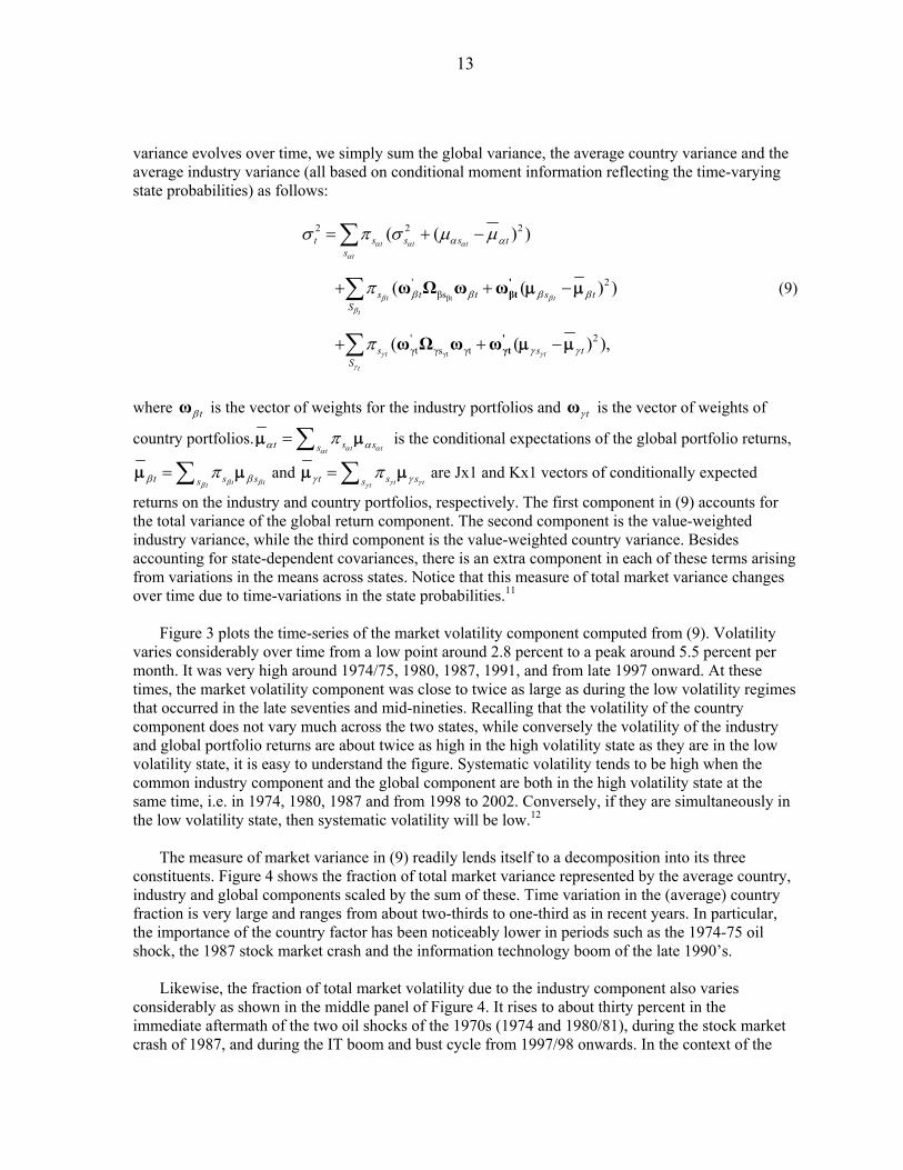
returns on the industry and country portfolios, respectively. The first component in (9) accounts for the total variance of the global return component. The second component is the value-weighted industry variance, while the third component is the value-weighted country variance. Besides accounting for state-dependent covariances, there is an extra component in each of these terms arising from variations in the means across states. Notice that this measure of total market variance changes over time due to time-variations in the state probabilities.11

Figure 3 plots the time-series of the market volatility component computed from (9). Volatility

varies considerably over time from a low point around 2.8 percent to a peak around 5.5 percent per month. It was very high around 1974/75, 1980, 1987, 1991, and from late 1997 onward. At these times, the market volatility component was close to twice as large as during the low volatility regimes that occurred in the late seventies and mid-nineties. Recalling that the volatility of the country component does not vary much across the two states, while conversely the volatility of the industry and global portfolio returns are about twice as high in the high volatility state as they are in the low volatility state, it is easy to understand the figure. Systematic volatility tends to be high when the common industry component and the global component are both in the high volatility state at the same time, i.e. in 1974, 1980, 1987 and from 1998 to 2002. Conversely, if they are simultaneously in the low volatility state, then systematic volatility will be low.12

The measure of market variance in (9) readily lends itself to a decomposition into its three

constituents. Figure 4 shows the fraction of total market variance represented by the average country, industry and global components scaled by the sum of these. Time variation in the (average) country fraction is very large and ranges from about two-thirds to one-third as in recent years. In particular, the importance of the country factor has been noticeably lower in periods such as the 1974-75 oil shock, the 1987 stock market crash and the information technology boom of the late 1990’s.

Likewise, the fraction of total market volatility due to the industry component also varies

considerably as shown in the middle panel of Figure 4. It rises to about thirty percent in the immediate aftermath of the two oil shocks of the 1970s (1974 and 1980/81), during the stock market crash of 1987, and during the IT boom and bust cycle from 1997/98 onwards. In the context of the

14

existing literature, the estimated average level in the 10 to 15 percent range is slightly higher than the 7 percent figure of Heston and Rouwenhorst (1994) and more than twice as high as the estimates in Griffin and Karolyi (1998)—both based on linear single-state models.13 Figure 4 clearly unveils significant changes in the relative importance of the industry factor and shows that its recent rise has in fact been the most persistent of all over the past thirty years, though not quite yet to the point where its contribution to volatility has surpassed that of the country factor. As shown in the bottom panel of Figure 4, this is partly due to the concomitant rise of the global factor contribution to overall stock return volatility in recent years which has filled some of the gap arising from the decline in country-specific volatility.

It is instructive to compare these results with those obtained through the widespread practice of

estimating relative contributions by the time-series variances of the estimated jtβ and ktγ , computed over a rolling window. We follow the common practice of using a window length of 3 years, but also experimented with 4- and 5-year rolling windows and found the trends to be very similar. To facilitate comparison with our results, Figure 5 plots the 3-year rolling window results together with our regime switching estimates previously plotted in Figure 4. Clearly, the rolling window approach smoothes out the shifts in factor volatilities and their relative contributions. The respective states become less clearly defined and the approach overlooks the important spikes associated with the oil shocks of 1973-74 and 1979-80.

Finally, we also consider an alternative and complementary measure of the relative significance

of the industry and country contributions to portfolio returns, which was proposed by Griffin and Karolyi (1998). Our two-stage econometric methodology allows us to extend the Griffin and Karolyi decomposition scheme by both letting the relative contributions of each factor vary across states and taking into account the various industry covariances within each state. As in Griffin and Karolyi (1998), let the excess return on the national stock market or portfolio of country k (over and above the global portfolio return α ) be decomposed into country k’s unique industry weights times the industry

returns summed across industries (i.e., 1

ˆJ

jkt jtj

βω β=∑ ) plus a “pure” country effect ˆktγ :14

1

ˆˆ ˆ ,J

kt t jkt jt ktj

R βα ω β γ=

− = +∑ (10)

where jkt

βω is the jth industry’s weight in country k. The variance of this excess return conditional on

the country state being tsγ and the industry state being tsβ is 'ˆ( | , ) ( ) ' 2( ) ' ( , | , ),

sskt t t t kt kt k k kt jt kt t ytVar R s s Cov s s

β γ γβ

β β ββ γ βα β γ− = + +ω Ω ω e Ω e ω (11)

where β

ktω is the J-vector of market capitalization weights of the industries in country k. Similarly, the excess return on the portfolio of industry j (over and above the global portfolio)

can be decomposed into industry 'j s unique country weights times the country returns summed

across countries plus a pure industry effect, ˆjtβ :

15

1

ˆˆ ˆ ,K

jt t jkt kt jtk

R γα ω γ β=

− = +∑ (12)

where jktγω is the kth country’s weight in industry j . The variance of this excess return conditional on

the country state being tsγ and the industry state being tsβ is

'ˆ( | , ) ( ) ' ( ) ' 2 ( , | , ),s

jt t t t jt jt j s j jt jt kt t ytVar R s s Cov s sγ βγ

γ γ γβ γ β βα β γ− = + +ω Ω ω e Ω e ω (13)

where kt

γω is the K-vector of market capitalization weights of the countries in industry j . Panel A in Table 6 reports the time-series variances of the “pure” country effects and the

cumulative sum of the industry effects in the 13 country portfolios, while Panel B reports the time-series variances of the pure industry effects and the cumulative sum of country effects in the 11 industry portfolios. In both cases, these variances are expressed as a ratio relative to the total variances of the excess returns. Their sum is therefore close, but not exactly equal to one due to the presence of the extra covariance term in (11) and (13) between the industry and country effects.

Since country volatility does not vary greatly over the two states, to save space Table 6 simply

presents results separately for the high and low industry volatility state. While a number of individual country and sector results are of interest in their own right, looking at the overall means, two findings stand out. First, the 3.3 percent figure reported in the upper right panel is the overall measure of the industry factor contribution in the low industry volatility state, which is well within the range previously estimated by Griffin and Karolyi (1998) (2 and 4 percent depending on the level of industry aggregation—see tables 2 and 3 of their paper). Turning to the left panel, however, one can see that the same measure yields a much higher estimate of the aggregate industry component in the country portfolios (22.3 percent on average). In both the high and low industry volatility states, the average pure country volatility accounts for over 90 percent of the total country volatility—the fact that the right- and the left-hand side estimates in Panel A add to 120 percent being due to the higher negative covariance between the pure country and the composite industry effect during the high industry volatility state.

Moving to the breakdown of the industry portfolios shown in the bottom panels of Table 6, it is

clear that the aggregate contribution of country effects to industry portfolios is also state sensitive, being much lower (17 percent) in the high industry volatility state than in the low industry volatility state where it more than doubles (41 percent). Similarly, the pure industry contribution accounts for 91 percent of the total industry portfolio volatility in the high industry volatility state but only for 69 percent in the low industry volatility state. These results therefore suggest that decomposition averages reported in previous studies do vary considerably over economic states. 5. Economic Interpretation: Oil, Money, and Tech Shocks The existence of distinct volatility regimes in stock returns and shifts in the factor contributions therein beg the question of what drives them. While the construction of a multivariate global risk model capable of identifying the various underlying shocks and their propagation into stock pricing is beyond this paper’s scope, it is important to relate the above findings to key global economic developments in light of an existing literature on the drivers of stock market volatility. Furthermore, this provides an additional robustness check on the reasonableness of our estimates.

16

A glance at the top and bottom panels of Figure 1 as well as Figure 3 is suggestive of one key

determinant of the three main spikes in global market volatility identified by our model – 1973-75, 1979-80, and 1986-87. These were periods when the probability of being in the high volatility state for the common industry factor peaked relative to the rest of the sample (bottom panel of Figure 1), and the industry factor’s contribution to overall global market volatility rose (middle panel of Figure 4). This clearly coincided with large oil shocks: oil prices tripled in 1974, more than doubled in 1979, and underwent a sharp decline in 1986, when the spot price of oil reached an in-sample trough below $10/barrel. These periods coincided with spells of substantial short-run volatility in oil prices and marked profitability shifts across industries depending on their oil-intensity, leading to greater uncertainty about future earnings growth that were also reflected in current stock prices (Guo and Kliesen, 2005; Kilian and Park, 2007).

Similar evidence that industry-specific shocks contributed to drive up global stock return volatility from 1997 is also evident from our estimates, which highlight the higher contribution of the industry factors during that period. Yet, a more complex set of circumstances appears to have been at play. To gain insight into those, Figure 7 plots the smoothed transition probabilities for the different industries. Earlier explanations of the rise in volatility and co-movement across mature stock markets during 1997-2001 focus on the IT sector (Brooks and Catão, 2000; Brooks and del Negro, 2004). This is not only because IT stock volatility rose sharply during those years but also because the weight of the sector in the global market portfolio more than doubled – from 10 percent in mid-1997 to 25 percent at the market peak in March 2000. As discussed by Ohlin and Sichel (2000), this coincided with efficiency gains in the information technology sector, an associated shift in the relative profitability across industries and frequent revisions in earnings growth expectations, all of which only became tangible – and not so gradually so – in the late 1990s because of a sharp rise in the sector’s weight. This is starkly picked up by our smoothed transition probability estimates shown in the second panel of Figure 7B.

However, our estimates indicate that such a transition into a higher volatility state is not the preserve of the IT sector. The post-1997 period was also characterized by rising volatility in oil prices: the world oil price tripled between end-1998 and end-2000, before dropping sharply through 2001 and shooting up subsequently. This is clearly captured by the transition probability estimates for the resource industry in Figure 7A. In addition, other industries also witnessed a volatility bout and these are not limited to media and telecom firms–industries with closer ties to the IT sector (grouped under cyclical and non-cyclical services, respectively – see footnote 5). Some of this generalized volatility rise no doubt reflects the well-known tightening in world monetary conditions and financial distress in Asian emerging markets and Russia, particularly affecting the financial service sector (which was more heavily exposed to those markets – cf.. the widely publicized collapse of the US-based hedge fund Long-Term Capital Management), but also large chunks of the general industry in the US, Japan and Europe which also exported heavily to those emerging markets (see Forbes and Chinn, 2004 on related evidence). Hence, it is not surprising that the model is picking up such a strong common industry component rapidly transitioning from a low to a high volatility state. In a nutshell, while previous work has emphasized the role of the IT sector in driving up global market volatility between 1997 and 2002, our industry estimates and the model’s allowance for a common industry factor indicate that the phenomenon was more widespread than previous work may suggest.

Our estimates also suggest that industry-specific shocks are not the whole story behind the successive ups and downs in global stock return volatility during 1973-2002. Specifically, industry-specific shocks do not seem able to account for two other volatility shifts which we identify – the

17

volatility upturns of 1982-83 and 1985. Both occasions, however, were marked by substantial volatility in a well-known determinant of stock returns such as the short-term (risk-free) interest rate (see Eichengreen and Tong (2004) and the various references therein). Reflecting monetary policy shocks in the US and also in countries like the UK – to which global real interest rates responded by rising to unprecedented levels (see Bernanke and Blinder, 1992 for a discussion on the “exogeneity” of such shocks), volatility in the 3-month US Treasury bill market rose sharply during those episodes.15 This is illustrated in Figure 6, which plots the intra-month volatility in the Treasury bond yields (calculated from daily data), together with the volatility of returns on the stock market indices of the thirteen countries comprising our sample. The correlation between the two indices is reasonably tight at such high frequencies, yielding a correlation coefficient of 0.42 between end-1981 and end-1985. The fact that such monetary policy shocks were dramatic and not-so-gradual is consistent the behavior of the smoothed state transition probability which clearly display changes in volatility states around those episodes that were discrete and non-gradual. 6. Implications for Global Portfolio Allocation

Our decompositions of market variance are based on the average country and industry-specific variances. As such, they are statistical measures that do not represent the payoffs from a portfolio investment strategy since they ignore covariances between the returns on the underlying country, industry, and global equity portfolios. The advantage of such measures is that they provide a clear idea of the relative size of the variances of returns on the three components (global, industry and country). International investors, however, will be interested in economic measures of volatility and risk that represent feasible investment strategies and hence account for covariances between returns on the different portfolios involved. Further, changes in these covariances have important implications. For instance, when such covariances increase, domestic risk becomes less diversifiable which in turn tends to raise the equity premium and drive up the cost of capital.

The large literature on the links between national stock markets finds that the covariance of

(excess) returns between national stock indices displays considerable variation over time (King, Sentana, and Wadhwani, 1994; Lin, Engle, and Ito, 1994; Bekaert and Harvey, 1995; Longin and Solnik, 1995; Karolyi and Stultz, 1996; Hartmann et al., 2004). In this section, we use firm level data and the methodology laid out in the previous sections to characterize the behavior of country portfolio covariances. Like King, Sentana, and Wadhwani (1994) and others, we let such time variation in country covariances be driven by an unobserved latent variable but, unlike those authors, we characterize such variations in terms of relatively lengthy historical periods or “states” and allow for differences in industry composition across countries to play a role. Likewise, the same approach is used to characterize the covariance patterns of the various industry portfolios. Because the estimated covariances/correlations within volatility states are conditional upon the entire time series information up to that point, they are not subject to the type of biases affecting unconditional estimates which have been highlighted by Forbes and Rigobon (2001). Moreover, an important spin-off of the proposed approach that, to be best of our knowledge has not been explored in the literature, is the possibility that the country and industry portfolios may be in different states at a given point in time, thus raising interesting possibilities for risk diversification.

To see this, recall that the joint models ((9)—(10)) assume separate state processes for the global

return factor (which affects all stocks in every period) and for the country or industry returns. Each of these state variables can be in the high or low volatility state. The return on a geographically diversified portfolio invested in industry j will be αt + βjt, while the return on an industrially

18

diversified country portfolio is αt + γkt. For such portfolios there are thus four possible state combinations. For the industry portfolios the four states are:

high industry volatility, high global volatility (sβt = 1; sαt = 1) high industry volatility, low global volatility (sβt = 1; sαt = 2) low industry volatility, high global volatility (sβt = 2; sαt = 1) low industry volatility, low global volatility (sβt = 2; sαt = 2)

The correlation between geographically diversified industry portfolios is likely to vary strongly according to the underlying combination of global and industry state variables. By construction, the global component is common to all stocks. Thus, when the global return variable is in the high volatility state, it will contribute relatively more to variations in the returns of such portfolios and correlations will increase. In contrast, when the global return component is in the low volatility state, correlations between country or industry portfolios will tend to be lower. Similarly, when the industry component is in the low volatility state, the relative significance of the common global return component is larger so that correlations between industry portfolios will be stronger compared to when the industry return process is in the high volatility state. Given the very large differences between volatilities in the high and low volatility states observed for the global and industry portfolios, these effects are likely to give rise to large differences between correlations of geographically diversified industry portfolios in the four possible states.

A complication arises when computing these correlations as they depend on the correlation

between the global and industry or country portfolio returns. Terms such as ),|,( ttktt ssCov γγα can be consistently estimated as follows:

1

1

1

1

1

ˆˆ( )( )( , | , ) ,

ˆ ˆ( )( )( , | , ) ,

ˆ ˆ( )( )( , | , )

t t t

t t

t t t

t

t t t t

t

Ts s t s jt jstt

t jt t t Ts st

Ts s t s kt kskt

t kt t t Ts s tt

Ts s jt js kt kst

t t t ts s

Cov s s

Cov s s

Cov s s

α α β

α β

α α γ

α

β γ β γ

β

βα β

γα γ

γ

β γ

π π α α β βα β

π π

π π α α γ γα γ

π π

π π β β γ γβ γ

π π

=

=

=

=

=

− −=

− −=

− −=

∑∑

∑∑

∑1

.Ttt γ=∑

(14)

To investigate just how different these correlations and volatilities are, Table 7 presents the

estimated covariances and correlations in the two possible states for the industrially diversified country portfolios, while Table 8 presents the estimated covariances and correlations for the geographically diversified industry portfolios. Variances are presented on the diagonals, covariances above the diagonal, and correlations are below.

For the country portfolios, the key findings are as follows. First, correlations across countries

vary substantially, even after allowing for cross-country differences in industry composition. In particular, correlations are generally higher among the Anglo-Saxon countries (notably between Canada, the United States, and the United Kingdom) and lowest between the United States and much of continental Europe and Japan. This result is consistent with the evidence of other studies using

19

different methodologies and measures (see, e.g., IMF, 2000) and our estimates show that it broadly holds across states.16 Second, correlations change markedly across states. Since there is not much difference between the variance of country returns in the high and low volatility states, the main driver of the results will be whether the global portfolio is in the high or low volatility state. The average correlation between the country portfolios is 0.30 in the low global volatility state and 0.56 in the high global volatility state. Thus, as other studies using distinct econometric methodologies and data series have found (see e.g. Solnik and Roulet, 2000; Bekaert, Harvey, and Ng, 2005), the state process for the global return component clearly makes a big difference to the average correlations between the country portfolios – our estimates for 13 mature markets indicating that such correlations almost double in the high volatility state.

Turning to the geographically diversified industry portfolios listed in Table 8, a richer menu of

possible combinations emerges since the global high and low volatility states are now supplemented by the high and low industry volatility states. When the industry process is in the high volatility state while the global process is in the low volatility state, the average correlation across industry portfolios is only 0.19. This rises to 0.50 when the industry and global processes are both in the high volatility state or both are in the low volatility state. Finally, when the industry state process is in the low volatility state while the global process is in the high volatility state, the average correlation across the geographically diversified industry portfolios is 0.81. These results show that the average correlations between geographically diversified industry portfolios vary substantially according to the state process driving the common industry component and the global component, with the non-negligible differences in industry factor correlations within each state being especially magnified in the high industry volatility state. Finally we note how different the average volatility level is in the high and low volatility states. For the country portfolios the variation in volatility is, unsurprisingly, somewhat smaller. The mean volatility is 6.4 percent per month in the high global volatility state and 5.3 percent in the low volatility state. The mean volatility of the industry portfolios is 6.6 percent per month in the high industry-, high global volatility state as compared with an average volatility of these portfolios of 3.6 percent in the low industry-, low global volatility state.

Important implications follow from these results. Generally, it will be more difficult to reduce

equity risk through cross-border diversification when the global volatility process is in the high volatility state. On a macro level, this suggests that international capital flows should be expected to rise or accelerate during periods of low global stock market volatility and to web during high volatility states. Moreover, as the gains to cross-border diversification appear to be especially meager when global and industry factors both simultaneously lie in a high volatility state, this suggests that cross-border risk diversification should not be so beneficial during those sub-periods. Provided that a country has a sufficiently diversified domestic industrial structure that allows residents to diversify risk along broad industry lines without having to go abroad, international equity flows will tend to be dampened as a result. This raises the question of whether these patterns are actually observed in the data. A systematic testing of this relationship is no mean task – not only because international capital flows are driven by a number of effects at play (see, e.g. Tesar and Werner, 1994), but also because of considerable data problems even if we were to limit the analysis to US data. Yet, it clearly warrants attention by future research. 7. Conclusion

This paper has developed a regime switching modeling framework and applied it to 30-year long

firm-level data to address three main questions – whether global stock return volatility displays well-

20

defined volatility regimes, the extent to which equity market volatility is accounted for by global, country- or sector-specific factors, and what implication this has for national equity market correlations and international risk diversification.

Our results reveal strong evidence of regimes in international stock returns characterized by

different levels of volatility, with the low volatility regime being two to three times more persistent once we average over the various individual country and industry portfolios. The robustness of these results is not only butressed by a variety of statistical tests on the model’s residuals but also by an identification of volatility regimes which is broadly consistent with estimates from alternative non-parametric measures, as well as with what we know about the timing of major shocks deemed to affect stock market volatility. At the very least, this suggests that the single-state assumption underlying the linear models used in previous studies can be improved upon. As discussed above and further stressed below, the inadequacy of the single-state assumption is not only a technical econometric issue: it also leads one to gloss over important shifts in portfolio diversification possibilities as the various factors switch between high and low volatility regimes over time. To the extent that such states are persistent enough to allow the respective probabilities to be estimated with reasonable precision, market participants should thus be able to reap significant benefits from monitoring the underlying state probabilities as well as cross-country and -industry portfolio correlations within them.

Since allowing for time- varying factor contributions appears to characterize the data better than

linear models with similar factor structure, this should also deliver more accurate estimates of the various factor contributions. Over the entire period 1973-2002 period, the country factor contribution averaged some 50 percent as opposed to 16 percent for the industry factor. Yet, these contributions have witnessed important variations across volatility states, with the country factor contribution dropping sharply at times, to as low as under 35 percent as around 1973-74, 1986-87 and 2000-01. Further, since each factor in the model is allowed to be in one of two states at any point in time, we also show that economically interesting state combinations arise as each combination gives rise to a stronger or weaker pattern of correlations between the various portfolios. In general, the correlations among the various country and industry portfolios are stronger in the high global volatility state than in the low global volatility state; in the case of industrially diversified country-specific portfolios, those correlations nearly double on average. Hence the diversification benefits of investing abroad tend to be considerably smaller when global volatility is high. Further, and also after accounting for different industrial make-ups across countries and differences in volatility regimes, pair-wise correlations between the various country portfolios indicate that international diversification benefits are even smaller when confined to certain subsets of countries, such as the Anglo-Saxon nations or within continental Europe.

These results speak directly to various strands of the literature. First, our findings suggest that the

apparently greater potential for industry diversification arising from the greater contribution of industry factors to stock return volatility between 1997 and 2002 is likely to be, at least in part, temporary: global stock market volatility typically goes through ups and downs and the contribution of country-factors typically declines (rises) during high (low) global volatility states; so, the incentive for global equity diversification along industry lines (as opposed to country lines) should shift accordingly – rather than being a permanent phenomenon. A similar inference follows from the evidence presented in Brooks and del Negro (2004) and Bekaert et al (2005) using different econometric approaches and distinct levels of industry disagregation in their discussion of the IT bubble of the late 1990s.

21

Second, related inferences can be drawn about the role of “globalization” in driving down the contribution of country factors in stock returns. While a number of studies have pointed to a decline in home bias and noted that firm operations (particularly among advanced countries) have grown more international (cf. Diermeier and Solnik, (2001)), our finding that the contribution of country factors have fluctuated throughout the period cautions against seeing the 1997-2002 decline as permanent due to “globalization” forces. This is not to exclude that this shift may have a sizeable permanent component especially for certain country sub-groups – notably in Europe (cf. Baele and Inghelbrecht, 2005). What our look at the historical evidence on regime shifts simply suggests is that the estimated longer stay in a low country volatility state plus the attendant decline in the contribution from the country factor from the mid-1990s may be picking up temporary as well as permanent factors. More definitely, our estimates also suggest that, in any event, greater globalization has not yet resulted in the industry factor becoming more important than the country factor. More time series data, together with richer structural models that pin down the various sources of market integration, are clearly needed before firmer inferences can be made about how permanent such shifts turn out to be.

Third, our estimates of “pure” country portfolio correlations across national stock markets are consistent with the findings of an emerging literature on information frictions or institutional-based “gravity” views of international equity flows (Portes and Rey, 2005). Because our estimates are conditional upon the distinct volatility states and use all the time series information up to that point, they are robust to the bias affecting unconditional correlations discussed in Forbes and Rigobon (2001), which plagues unconditional correlations reported in much of the literature. As in such gravity-type models, these conditional correlation estimates clearly show that market correlations tend to be systematically higher – both during high and low volatility states – among Anglo-Saxon countries and across much of continental Europe. An open question for future research is to which extent higher “pure” country correlations among European countries have intensified over time and on a permanent basis since the introduction of the euro in 1999 and of other regional harmonization policies – rather than resulting from the rise in the global factor-driven volatility since 1997.

Finally, interesting implications for the pattern of cross-border capital flows also follow. For one

thing, evidence that over the long run average stock return volatility has been mainly determined by country-specific factors suggests that equity risk can be greatly reduced by diversifying portfolios across national borders. This provides an important rationale for the observed dramatic growth in gross cross-border equity holdings which, in turn, has important implications for international macroeconomic adjustment (Lane and Milesi-Ferretti, 2001). Conversely, however, during high global and high industry volatility regimes (such as those historically associated with large sector-specific shocks such as oil), the risk diversification incentive to cross-border flows is therefore weakened and perceived home bias is strengthened. Even granting that risk diversification is simply one among other potential drivers of cross-border flows, one’s allowance for the existence of such regime shifts may shed new light on the question of what drives the massive swings in the growth of cross-border equity holdings observed in the data. While further research considering a host of other factors and based on better equity flow data is clearly needed before any robust inference is drawn, this hypothesis emerges as an interesting spin-off of this paper’s results.

22

References Ammer, John and Jon Wongswan, 2004, “Cash Flows and Discount Rates, Industry and Country

Effects, and Co-Movement in Stock Returns,” Board of Governors of the Federal Reserve System, International Finance Discussion Papers 818.

Ang, Andrew and Geert Bekaert, 2002, “International Asset Allocation with Regime Shifts,” Review

of Financial Studies, 15, 1137-87. Baele, Lieven and Koen Inghelbrecht, 2005, “Time-Varying Integration and International

Diversification Strategies”, Tilburg University, unpublished manuscript. Bekaert, Geert and Campbell Harvey, 1995, “Time-Varying World Market Integration,” Journal of

Finance 50, 403-44. ________, Campbel Harvey, and Angela Ng, 2005, “Market Integration and Contagion,” Journal of

Business 78, 39-70. ________, Robert Hodrick, and Xiaoyan Zhang, 2005, “International Stock Return Comovements,”

NBER working paper 11906 Beckers, Stan, R. Grinold, A. Rudd, and D. Stefek, 1992, “The Relative Importance of Common

Factors Across the European Equity Markets,” Journal of Banking and Finance, Vol. 16, pp. 75–95.

Bernanke, Ben and Alan Blinder, 1992, “The Federal Funds Rate and the Channels of Monetary

Transmission”, American Economic Review, 82(4), pp. 901-921. Brooks, Robin and Luis Catão, 2000, “The New Economy and Global Stock Returns”, IMF working

paper 00/216, Washington: International Monetary Fund. ______ and Marco del Negro, 2002,”International Diversification Strategies”, Working paper 2002-

23, Federal Reserve Bank of Atlanta. Campbell, John, Andrew W. Lo and A. Craig Mackinlay, 1997, The Econometrics of Financial

Markets, Princeton. Cavaglia, Stefano, C. Brightman and M. Aked, 2000, “The Increasing Importance of Industry

Factors”, Financial Analysts Journal, pp.41-54. Davies, R., 1977, “Hypothesis Testing When a Nuisance Parameter is Present Only Under the

Alternative,” Biometrica, Vol. 64, p. 247–254. Diemeier, J. and Bruno Solnik, 2001, “Global Pricing of Equity”, Financial Analysts Journal 57, pp.

37-47. Driffill, John and Martin Sola, 1994, “Testing the Term Structure of Interest Rates from a Stationary

Switching Regime VAR,” Journal of Economic Dynamics and Control Vol. 18, pp. 601–628.

23

Eichengreen, Barry and Hui Tong, 2004, “Stock Market Volatility and Monetary Policy: What the Historical Record Shows,” Paper presented at the Central Bank of Australia.

Engel, Charles and James D. Hamilton, 1990, “Long Swings in the Dollar: Are they in the Data and

do the Markets Know it?”, American Economic Review 80, 689-713. Frisch, Ragnar, 1933, “Propagation and Impulse Problems in Dynamic Economics,” Essays in Honor

of Gustav Cassel, London. Forbes, Kristin and Roberto Rigobon, 2001, “No Contagion, Only Interdependence: Measuring Stock

Market Co-Movements,” Journal of Finance 57, Number 5, pp 2223-2261. _________ and Menzie Chinn, 2004, “A Decomposition of Global Linkages in Financial Markets

Over Time”, Review of Economics and Statistics, 86(3), pp.705-722. Griffin, John and G. Andrew Karolyi, 1998, “Another Look at The Role of Industrial Structure of

Markets for International Diversification Strategies,” Journal of Financial Economics 50, pp. 351–373.

Griffin, John and Rene Stultz, 2001, “International Competition and Exchange Rate Shocks: A Cross-

country Industry Analysis,” Review of Financial Studies 14, pp.215-241. Guo, Hui and Kevin Kliesen, 2005, “Oil Price Volatility and U.S. Macroeconomic Activity”, Federal

Reserve Bank of St. Louis Review, Nov/Dec., pp. 669-683. Hamilton, James, 1988, “Rational Expectations Econometric Analysis of Changes in Regime: An

Investigation of the Term Structure of Interest Rates,” Journal of Economic Dynamics and Control, Vol. 12, pp. 365–423.

———, 1989, “A New Approach to the Economic Analysis of Nonstationary Time Series and the

Business Cycle,” Econometrica 57, 357–384. ———, 1994, Time Series Analysis, Princeton. Hartmann, P., Straetmans, S., and de Vries, C. G., 2004, “Asset market linkages in crisis periods”,

Review of Economics and Statistics, 86(1), pp.313-326. Heston, Steven L. and K. Geert Rouwenhorst, 1994, “Does Industrial Structure Explain the Benefits

of International Diversification,” Journal of Financial Economics 36, 3–27. International Monetary Fund, 2000, “World Economic Outlook – Asset Prices and the Business

Cycle,” Washington D.C.: International Monetary Fund. Karolyi, Andrew and René Stultz, 1996, “Why do Markets Move Together? An Investigation of U.S.-

Japan Stock Return Comovements”, Journal of Finance 51, 951–86. Kilian, Lutz and Chealbeam Park, “The Impact of Oil Prices on the US Stock Market,” CEPR

discussion paper 6166.

24

Kim, Chang-Jin and Charles R.Nelson, 1999, State-Space Models with Regime Switching. Classical and Gibb-Sampling Approaches with Applications, Cambridge, Mass.

King, Mervin, Enrique Sentana, and Sushil Wadhwani, 1994, “Volatility and Links Between National

Stock Markets,” Econometrica 62, 901–33. Lane, Philip R. and Gian Maria Milesi-Ferretti, 2001, The external wealth of nations: measures of

foreign assets and liabilities for industrial and developing countries,” Journal of International Economics 55, 263-294

L’Her, J.F., O. Sy, and Y.Tnani, 2002, “Country, Industry, and Risk Factor Loadings in Portfolio

Management, Journal of Portfolio Management,28, 70-79. Lin, Weng-Ling, Robert F. Engle, and Ito Takatoshi, 1994, “Do Bull and Bears Move Across

Broders? Transmission of International Stock Returns and Volatility,” Review of Financial Studies 7, 507–538.

Longin, François and Bruno Solnik, 1995, “Is the Correlation in International Equity Returns Constant: 1970-1990,” Journal of International Money and Finance 14, 3-26. Oliner, Stephen and Daniel Sichel''The Resurgence of Growth in the late 1990s: Is Information

Technology the Story?'', Journal of Economic Perspectives, vol. 14 (Fall 2000), pp. 3-22. Pagan, Adrian and G.William Schwert, 1990, “Alternative Models for Conditional Stock Volatility,”

Journal of Econometrics 92, 307–28. Perez-Quiros, Gabriel and Allan Timmermann, 2000, “Firm Size and Cyclical Variations in Stock

Returns,” Journal of Finance 55, 1229–62.

Portes, Richard and Helène Rey, 2005, “The Determinants of Cross-Border Equity Flows,” Journal of International Economics 65, 269-96.

Rigobon, Roberto and Brian Sack, 2003, “Measuring the Reaction of Monetary Policy to the Stock

Market”, Quarterly Journal of Economics, pp.639-669. Schwert, William, G., 1989, “Why Does Stock Market Volatility Change Over Time?”, Journal of

Finance 44, pp. 1115–1153. Solnik, Bruno, and Jacques Roulet, 2000, “Dispersion as Cross-Sectional Correlation,” Financial

Analysts Journal 56, 54–61. Stock, James and Mark Watson, 1998, “Diffusion Indexes,” NBER working paper 6702, Cambridge,

Mass.: National Bureau of Economic Research. Tesar, Linda and Werner, I, 1994, “International Equity Transactions and U.S. Portfolio Choice,” in

Frankel, J. (ed.), The Internationalization of Equity Markets, Chicago. Timmermann, Allan, 2000, “Moments of Markov Switching Models,” Journal of Econometrics 96,

75–111.

25

Notes to Main Text: 1 The two studies using the longest time series that we are aware of are Brooks and del Negro (2002) and Bekaert, Hodrick, and Zhang (2005). The sample coverage is 1985:1 to 2002:2 in the former, and 1980:1 to 2003:12 in the latter. Thus, none of these studies incorporates in their estimates the effects of the large shifts in stock market volatility and relative factor contribution following the oil shocks and monetary disturbances of the 1970s, which we document. We return to this issue below.

2 Besides its popularity, there are three particular reasons why we retain this three-factor specification. First, we are interested in country and industry effects in their own right and we know that a model with both country and industry factors systematically dominates one with country- or with industry factors alone (see Bekaert, Hoddrick, and Zhang, 2005 for a comparison of models with distinct factors). Second, adding a “small cap” factor or a similar proxy related to firm size has been shown to have negligible effects on country-industry decompositions for a similar sample of international firms (Catão and Brooks, 2000). Third, while regional factors are deemed to be important – in particular for Europe (cf. Baele and Inghelbrecht, 2005) – augmenting the model with various regional dummies would be infeasible due to degrees of freedom limitations arising from the richly parameterized nature of our regime switching specification in the second stage estimation. As time goes by and longer time series data become available, however, augmenting the model with regional factors could become a feasible extension to this model. 3 This is clear from the evidence presented in Brooks and del Negro (2002) who, after allowing for distinct firm-specific loadings, obtain very similar inferences about the relative factor contributions as those yielded when the homogeneity of factor loadings is imposed. As elsewhere in this literature, their results are based on the assumption of a single volatility state. Another important trade-off of allowing for firm-specific factor loadings (which are estimated by a maximum likelihood algorithm as in their study), is that of having to balance the panel since the algorithm cannot handle missing observations. As discussed above, by eliminating new firm entry and exit from the sample, this panel-balancing proceedure is an additional source of potential estimation biases. More recently, Bekaert, Hodrick and Zhang (2005) compared the performance of several models, including the Heston and Rouwenhorst (1994) model with fixed cross-sectional and time-series loads over shorter sub-periods. While Bekaert, Hodrick and Zhang (2005) find that an APT model incorporating both global and local factors fits the covariance structure of stock returns best, their results are restricted to the linear (one-state) version of the model. No less importantly, their study also finds that differences in the measurement of country vs. industry contributions between other (one-state) models and the Heston and Rouwenhorst one are mainly due to the time dimension of the sample, rather than to the assumption of unit beta loadings across firms. 4 Monthly total returns are computed in local currency using data from Datastream/Primark. The return calculation assumes immediate reinvestment of dividends. These local currency returns are converted to U.S. dollars using end-of-month spot exchange rates. The beginning-of-month stock market capitalizations are converted into U.S. dollars using the beginning-of-month dollar price of one unit of local currency. Expressing all returns and market cap data in US dollars implicitly reflects the perspective of a currency unhedged equity investor whose objective is to maximize U.S. dollar returns. To the extent that changes in equity returns overwhelm those associated with currency fluctuations, expressing returns and market caps in the distinct national currencies should not change the thrust of the results, as earlier work using a subset of this data has found (Brooks and Catão, 2000). This is consistent with what other researchers have also found using other datasets (Heston and Rouwenhorst, 1994; Griffin and Karolyi, 1998; Griffin and Stultz, 2001). One possible reason lies in

26

exchange rate hedging used by many large firms in developed countries with extensive international operations, which comprise a sizeable portion of those datasets. Developing country firms were excluded from the sample altogether because none of those reported in the Datastream/Primark dataset had sufficiently long series, entailing a too short time span for the respective country portfolio to be included the estimation of the Markov-switching regressions. 5 While Griffin and Karolyi (1998) note that a finer industry disaggregation may yield a more accurate measure of industry effects, their main result – the far greater dominance of country-specific effects—hardly changes with the move to a finer industry breakdown. An alternative breakdown which groups IT with media and telecoms under a broader TMT group has been considered in Brooks and Catão (2000) and Brooks and del Negro (2004) which show that the dynamics of the broader TMT group is largely dominated by the IT sector from 1990s. In the FTSE industry classification used in this paper, media is grouped under cyclical services and telecomunications under non-cyclical services. 6 For a sub-sample including dead firms, Brooks and del Negro (2002) obtain the following figures for the capitalization-weighted time-series variance of country effects (also gauged by the same parameter ktγ in the Heston-Rouwenhorst decomposition scheme): 18.47 over 1986:3 to 1990:2; 21.08 over 1990:3 to 1994:2; and 9.12 between 1994:3 and 1998:2. Using the same 4-year fixed windows and a similar group of mature markets but without including dead stocks, our respective estimates are 19.21, 22.10, and 8.80. So, the differences are small and have no discernable effect on trends. 7 The only reason the averages are not exactly equal to zero is that we are reporting arithmetic averages whereas the world portfolio is based on capitalization-weighted returns. 8 Section 3.C below reports the results of the normality tests for our fitted model, which show that residuals become broadly normal once conditioned on the regime moments, thus providing strong support for the proposed regime switching approach. 9 The finding of a single state for Canada and Switzerland is consistent with the Davies’ tests in Table 2 which could not reject linearity for these two countries. 10 Since the joint country model has 210 parameters while the joint industry model has 156 parameters (most of which measure the covariance between industry returns in the two states), we do not report all the estimates and instead concentrate on the standard deviations. 11 The squared terms in the variance expression enter due to the binomial nature of the state variable, c.f. Timmermann (2000). 12 Overall, our estimates plotted in Figure 3 suggest that systematic volatility is about trendless: if a trend is fitted into this measure of market variance (which excludes firm-level idiosyncratic variance as in equation (9)), it is very mildly positive and its statistical significance is quite sensitive to end point. A similar inference obtains when applying the non-parametric measure of intra-monthly volatility discussed in Section 3.C and plotted in Figure 2: the respective slope of regressing this volatility measure on a linear trend is positive (0.0001) but not statistically significant at 5%. This is consistent with Schwert’s (1989) finding for the US that market volatility does not display a significant long-term trend. Using, however, aggregate stock price data spanning over a century for

27

various advanced countries, Eichengreen and Tong (2004) suggest that stock market volatility displays a U-shape in most countries. It remains to be established whether this result stems from their use of much longer data series, the effects of idiosyncratic variance (which they do not filter out), or due to their methodology based on rolling standard deviations of stock price changes and univariate Garch(1,1) regressions. 13 Griffin and Karolyi (1998) present two sets of estimates, one using a nine-sector breakdown and the other using a 66 industry breakdown. They find that the mean industry factor contribution to total return variance are 2 and 4 percent respectively, a lot lower therefore than the above estimates. One possible reason for the lower estimate of Griffin and Karolyi (1998) relative to Heston and Rouwenhorst (1994) as well as ours is the inclusion of emerging markets in their sample. As country-specific shocks have been shown to play a greater role in the determination of stock returns in emerging markets, this is to be expected. However, we show below that much of the difference appears to be model and time dependent. Furthermore, Griffin and Karolyi consider a much shorter sample of weekly returns so differences in estimates are not all that surprising. 14 It is straightforward to show that this decomposition follows from re-writing equation (2) for each individual country portfolio, where the individual firm’s weight is the share of that firm in total market capitalization of the respective country portfolio. 15 Other high global volatility spells which overlap with changes in monetary policy stances and higher money market volatility are observed following the 1998 Russias crisis, the March 2000 stock market crash, and between late 2001 and early 2002, in the wake of September 11th terrorist attacks. As shown in Figure 6, however, none of these money market volatility bouts were of similar magnitude as those of the late 1970s and early 1980s. In this more recent period, there is also some evidence that monetary policy has become more reactive to the stock market (cf. IMF, 2000; Rigobon and Sack, 2003) and therefore a less independent driver of stock market volatility. This plausibly reflects the much greater weight of the stock market in aggregate wealth from the 1990s (relative to the 1970s and early 1980s), calling for greater attention of policy makers to stock market developments and their impact on aggregate spending and hence on price stability. 16 Among continental European countries, a main exception is the Netherlands whose country factor volatility is highly correlated with those of the US and the UK.

28

Figure 1. Smoothed State Probabilities for Common Components (High Volatility State)

Global

0.00

0.20

0.40

0.60

0.80

1.00

1973 1974 1976 1977 1978 1979 1981 1982 1983 1984 1986 1987 1988 1989 1991 1992 1993 1994 1996 1997 1998 1999 2001 2002

Common Country

0.00

0.20

0.40

0.60

0.80

1.00

1973 1974 1976 1977 1978 1979 1981 1982 1983 1984 1986 1987 1988 1989 1991 1992 1993 1994 1996 1997 1998 1999 2001 2002

Common Industry

0.00

0.20

0.40

0.60

0.80

1.00

1973 1974 1976 1977 1978 1979 1981 1982 1983 1984 1986 1987 1988 1989 1991 1992 1993 1994 1996 1997 1998 1999 2001 2002

29

Figu

re 2

. Act

ual I

ntra

-mon

thly

Var

ianc

e of

Sto

ck R

etur

ns a

nd M

S E

stim

ates

0.0

1.0

2.0

3.0

4.0

5.0

6.0

Mar-75

Mar-76

Mar-77

Mar-78

Mar-79

Mar-80

Mar-81

Mar-82

Mar-83

Mar-84

Mar-85

Mar-86

Mar-87

Mar-88

Mar-89

Mar-90

Mar-91

Mar-92

Mar-93

Mar-94

Mar-95

Mar-96

Mar-97

Mar-98

Mar-99

Mar-00

Mar-01

Mar-02

00.1

0.2

0.3

0.4

0.5

0.6

0.7

0.8

0.9

1In

tra-m

onth

ly v

aria

nce

MS

Glo

bal V

aria

nce

MS

Smoo

thed

pro

babi

lity

(rig

ht a

xis)

30

Figu

re 3

. Mar

ket V

olat

ility

Syst

emat

ic V

olat

ility

2.80

3.30

3.80

4.30

4.80

5.30

1973

197

4 19

76 1

977

1978

197

9 19

8019

8119

8319

8419

8519

8619

8719

8819

9019

9119

92 1

993

1994

1995

1997

1998

1999

2000

2001

31

Figure 4. Decomposition of Systematic Variance into Country, Industry and Global Factors

Variance due to country factor

0.30

0.35

0.40

0.45

0.50

0.55

0.60

0.65

1973 1974 1975 1976 1978 1979 1980 1981 1983 1984 1985 1986 1988 1989 1990 1991 1993 1994 1995 1996 1998 1999 2000 2002

Variance due to industry factor

0.00

0.05

0.10

0.15

0.20

0.25

0.30

0.35

0.40

0.45

1973 1974 1976 1977 1979 1981 1982 1984 1985 1987 1988 1990 1992 1993 1995 1996 1998 2000 2002

Variance due to global factor

0.15

0.20

0.25

0.30

0.35

0.40

0.45

0.50

1973 1974 1975 1976 1978 1979 1980 1981 1983 1984 1985 1986 1988 1989 1990 1991 1993 1994 1995 1996 1998 1999 2000 2002

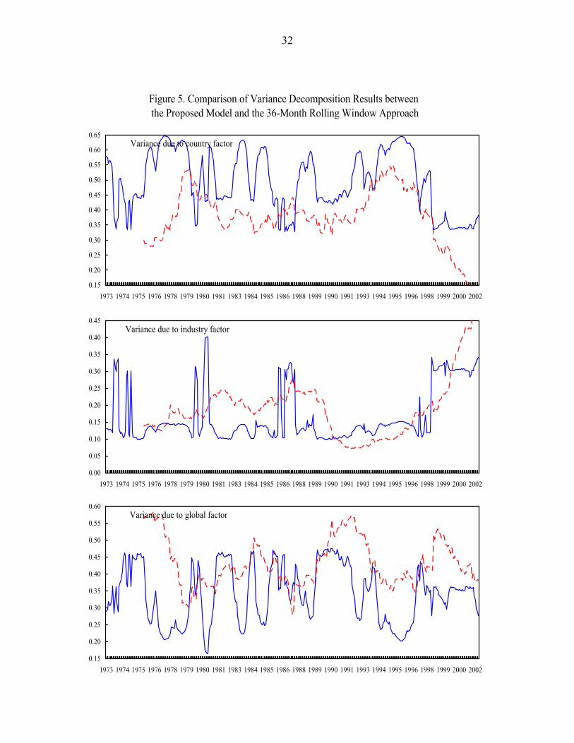
32

Figure 5. Comparison of Variance Decomposition Results between the Proposed Model and the 36-Month Rolling Window Approach

Variance due to country factor

0.15

0.20

0.25

0.30

0.35

0.40

0.45

0.50

0.55

0.60

0.65

1973 1974 1975 1976 1978 1979 1980 1981 1983 1984 1985 1986 1988 1989 1990 1991 1993 1994 1995 1996 1998 1999 2000 2002

Variance due to industry factor

0.00

0.05

0.10

0.15

0.20

0.25

0.30

0.35

0.40

0.45

1973 1974 1975 1976 1978 1979 1980 1981 1983 1984 1985 1986 1988 1989 1990 1991 1993 1994 1995 1996 1998 1999 2000 2002

Variance due to global factor

0.15

0.20

0.25

0.30

0.35

0.40

0.45

0.50

0.55

0.60

1973 1974 1975 1976 1978 1979 1980 1981 1983 1984 1985 1986 1988 1989 1990 1991 1993 1994 1995 1996 1998 1999 2000 2002

33

F

igur

e 6.

Intr

a-M

onth

ly V

aria

nce

of S

tock

Ret

urns

and

of t

he 3

-mon

th T

reas

ury

Bill

yie

ld

012345678910 1975

M2

1977

M1

1978

M12

1980

M11

1982

M10

1984

M9

1986

M8

1988

M7

1990

M6

1992

M5

1994

M4

1996

M3

1998

M2

2000

M1

2001

M12

0.0

0.1

0.2

0.3

0.4

0.5

0.6

0.7

0.8

0.9

1.0

Stoc

k R

etur

ns3-

mon

th T

Bill

(rig

ht a

xis)

34

Figure 7.A. Smoothed State Probabilities for Individual Industries(High Volatility State)

Resources

0.00

0.20

0.40

0.60

0.80

1.00

1973 1975 1976 1977 1979 1980 1982 1983 1985 1986 1987 1989 1990 1992 1993 1994 1996 1997 1999 2000 2002

Basic

0.00

0.20

0.40

0.60

0.80

1.00

1973 1975 1976 1977 1979 1980 1982 1983 1985 1986 1987 1989 1990 1992 1993 1994 1996 1997 1999 2000 2002

General Industry

0.00

0.20

0.40

0.60

0.80

1.00

1973 1975 1976 1977 1979 1980 1982 1983 1985 1986 1987 1989 1990 1992 1993 1994 1996 1997 1999 2000 2002

Cyclical Consumer Durables

0.00

0.20

0.40

0.60

0.80

1.00

1973 1975 1976 1977 1979 1980 1982 1983 1985 1986 1987 1989 1990 1992 1993 1994 1996 1997 1999 2000 2002

Non-Cyclical Consumer Durables

0.00

0.20

0.40

0.60

0.80

1.00

1973 1975 1976 1977 1979 1980 1982 1983 1985 1986 1987 1989 1990 1992 1993 1994 1996 1997 1999 2000 2002

35

Figure 7.B. Smoothed State Probabilities for Individual Industries(High Volatility State)

Utilities

0.00

0.20

0.40

0.60

0.80

1.00

1973 1975 1976 1977 1979 1980 1982 1983 1985 1986 1987 1989 1990 1992 1993 1994 1996 1997 1999 2000 2002

Information Technology

0.00

0.20

0.40

0.60

0.80

1.00

1973 1975 1976 1977 1979 1980 1982 1983 1985 1986 1987 1989 1990 1992 1993 1994 1996 1997 1999 2000 2002

Financials

0.00

0.20

0.40

0.60

0.80

1.00

1973 1975 1976 1977 1979 1980 1982 1983 1985 1986 1987 1989 1990 1992 1993 1994 1996 1997 1999 2000 2002

Non-cyclical Services

0.00

0.20

0.40

0.60

0.80

1.00

1973 1975 1976 1977 1979 1980 1982 1983 1985 1986 1987 1989 1990 1992 1993 1994 1996 1997 1999 2000 2002

Cyclical Services

0.00

0.20

0.40

0.60

0.80

1.00

1973 1975 1976 1977 1979 1980 1982 1983 1985 1986 1987 1989 1990 1992 1993 1994 1996 1997 1999 2000 2002

36

Table 1: Summary Statistics for the Country, Industry, and World Portfolio Returns

mean s.d. skew kurtosis

A. Country portfolios US -0.12 2.77 -0.42 2.48 UK 0.07 5.07 1.81 14.8 France 0.10 5.25 0.27 1.32 Germany -0.29 5.02 -0.09 0.81 Italy -0.12 7.28 0.38 1.71 Japan 0.11 4.63 0.02 0.58 Canada -0.29 3.85 -0.34 0.55 Australia -0.15 6.27 -0.25 1.67 Belgium -0.22 4.65 0.60 1.87 Denmark -0.10 5.32 0.33 1.33 Ireland 0.18 6.11 0.55 2.72 Netherlands -0.12 3.31 -0.04 1.02 Switzerland -0.28 4.04 -0.02 0.09

Average -0.09 4.89 0.22 2.38 B. Industry portfolios

Resources -0.12 3.74 0.03 0.88 Basic -0.19 2.52 0.06 3.71 General industry -0.05 1.78 -0.40 1.24 Cyclical durables -0.09 3.24 -0.30 1.22 Non-cycl. durables -0.05 2.45 -0.51 4.27 Cyclical services -0.06 1.61 0.01 0.68 Non-cycl. Services -0.17 3.72 0.88 3.11 Utilities -0.28 4.07 0.93 6.46 Information technology 0.18 4.34 0.50 3.01 Financials 0.00 2.28 -0.16 4.78 Others -0.51 2.79 0.21 2.62

Average -0.12 2.96 0.11 2.91 C. World: 1.71 4.34 -0.04 0.79

Notes: This table reports descriptive statistics for the country, industry and global portfolios using the decomposition (2) subject to the constraints (3), (4). Returns are measured at the monthly frequency over the period February 1973 – February 2002 and are based on a data set covering up to 3,951 firms in developed stock markets.

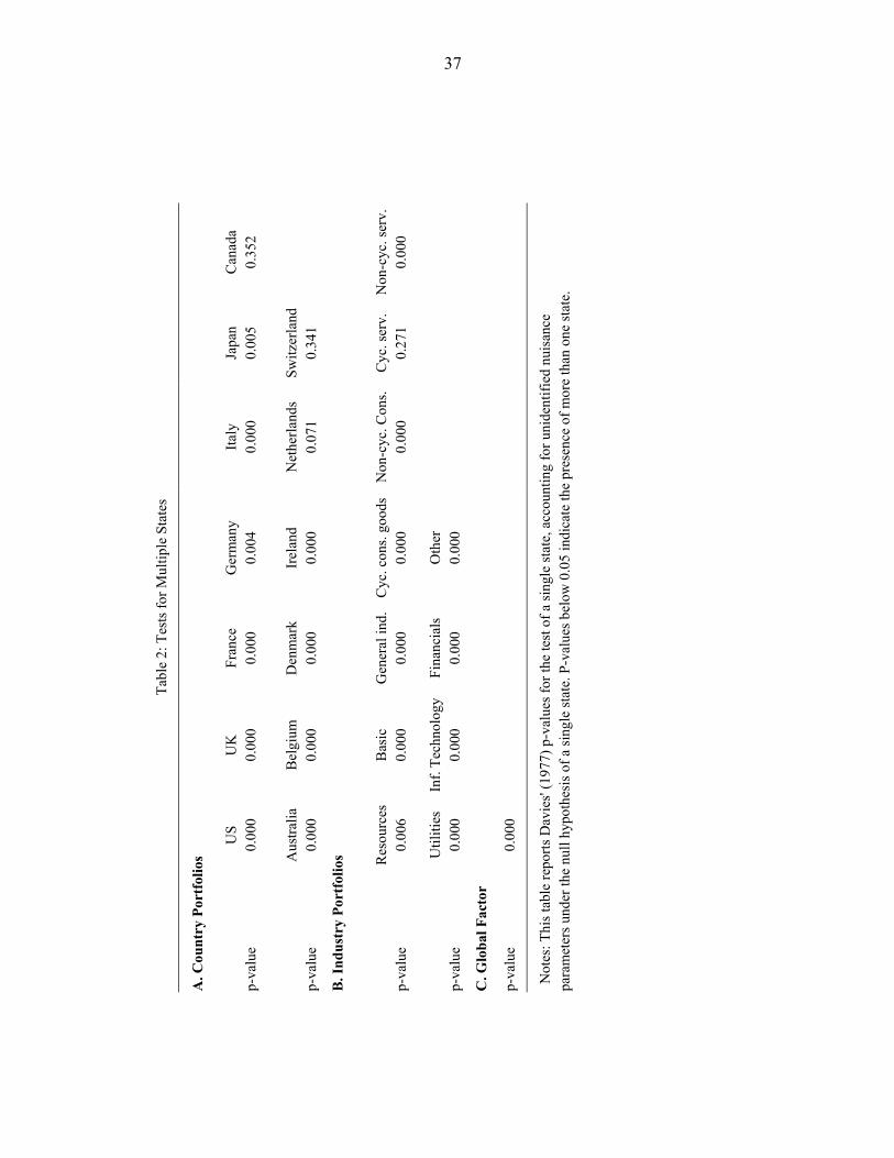
37

Ta

ble

2: T

ests

for M

ultip

le S

tate

s

A. C

ount

ry P

ortf

olio

s

U

S U

K

Fran

ce

Ger

man

y Ita

ly

Japa

n C

anad

a p-

valu

e 0.

000

0.00

0 0.

000

0.00

4 0.

000

0.00

5 0.

352

A

ustra

lia

Bel

gium

D

enm

ark

Irel

and

Net

herla

nds

Switz

erla

nd

p-va

lue

0.00

0 0.

000

0.00

0 0.

000

0.07

1 0.

341

B. I

ndus

try

Port

folio

s

R

esou

rces

B

asic

G

ener

al in

d.C

yc. c

ons.

good

s N

on-c

yc. C

ons.

Cyc

. ser

v.

Non

-cyc

. ser

v.p-

valu

e 0.

006

0.00

0 0.

000

0.00

0 0.

000

0.27

1 0.

000

U

tiliti

es

Inf.

Tech

nolo

gy

Fina

ncia

ls

Oth

er

p-

valu

e 0.

000

0.00

0 0.

000

0.00

0

C. G

loba

l Fac

tor

p-va

lue

0.00

0

Not

es: T

his t

able

repo

rts D

avie

s' (1

977)

p-v

alue

s for

the

test

of a

sing

le st

ate,

acc

ount

ing

for u

nide

ntifi

ed n

uisa

nce

para

met

ers u

nder

the

null

hypo

thes

is o

f a si

ngle

stat

e. P

-val

ues b

elow

0.0

5 in

dica

te th

e pr

esen

ce o

f mor

e th

an o

ne st

ate.

38

Tabl

e 3:

Sel

ectio

n C

riter

ia fo

r Ind

ivid

ual C

ount

ry, I

ndus

try, a

nd G

loba

l Por

tfolio

s

A

IC

B

IC

H

-Q

k =

1 k

= 2

k =

3 K

= 1

k

= 2

k =

3 k

= 1

k =

2 k

= 3

A

. Cou

ntry

Por

tfol

ios

US

4.88

2 4.

700

4.72

8 4.

904

4.76

7 4.

860

4.89

1 4.

727

4.78

0

UK

6.

093

5.80

3 5.

720

6.11

5 5.

869

5.85

2 6.

101

5.82

9 5.

773

Fr

ance

6.

163

6.04

5 6.

050

6.18

5 6.

111

6.18

2 6.

172

6.07

1 6.

102

G

erm

any

6.07

4 6.

049

6.06

9 6.

096

6.11

5 6.

201

6.08

3 6.

075

6.12

1

Italy

6.

817

6.73

1 6.

750

6.83

9 6.

798

6.88

2 6.

826

6.75

8 6.

802

Ja

pan

5.91

0 5.

886

5.89

4 5.

932

5.95

2 6.

027

5.91

9 5.

912

5.94

7

Can

ada

5.54

3 5.

549

5.55

9 5.

565

5.61

5 5.

693

5.55

2 5.

575

5.61

3

Aus

tralia

6.

518

6.43

5 6.

455

6.54

0 6.

501

6.58

7 6.

526

6.46

1 6.

508

B

elgi

um

5.92

0 5.

856

5.86

1 5.

942

5.92

3 5.

994

5.92

8 5.

883

5.91

4

Den

mar

k 6.

189

6.13

3 6.

151

6.21

1 6.

199

6.28

4 6.

197

6.16

0 6.

204

Ir

elan

d 6.

468

6.32

7 6.

306

6.49

0 6.

393

6.43

8 6.

477

6.35

4 6.

359

N

ethe

rland

s 5.

241

5.23

5 5.

250

5.26

3 5.

301

5.38

3 5.

250

5.26

1 5.

303

Sw

itzer

land

5.

640

5.64

6 5.

660

5.66

3 5.

712

5.79

3 5.

649

5.67

2 5.

713

B

. Ind

ustr

y Po

rtfo

lios

Res

ourc

es

5.48

5 5.

462

5.35

6 5.

507

5.52

8 5.

488

5.49

3 5.

488

5.40

9

Bas

ic

4.69

7 4.

514

4.49

0 4.

719

4.58

1 4.

623

4.70

6 4.

541

5.54

3

Gen

eral

indu

stry

4.

000

3.89

3 3.

907

4.02

2 3.

959

4.04

0 4.

009

3.92

0 3.

960

C

yclic

al c

onsu

mer

goo

ds

5.20

0 5.

120

5.11

0 5.

222

5.18

5 5.

242

5.20

9 5.

145

5.16

3

Non

-cyc

lical

con

sum

er g

oods

4.

638

4.34

0 4.

359

4.66

0 4.

407

4.49

2 4.

647

4.36

7 4.

412

C

yclic

al se

rvic

es

3.79

5 3.

798

3.76

8 3.

817

3.86

5 3.

900

3.80

3 3.

825

3.82

1

Non

-cyc

lical

serv

ices

5.

473

5.39

6 5.

373

5.49

5 5.

462

5.50

6 5.

482

5.42

2 5.

426

U

tiliti

es

5.65

3 5.

448

5.46

3 5.

675

5.51

4 5.

595

5.66

2 5.

474

5.51

6

Info

rmat

ion

tech

nolo

gy

5.78

3 5.

484

5.46

0 5.

805

5.55

0 5.

593

5.79

2 5.

510

5.51

3

Fina

ncia

ls

4.49

4 4.

225

4.22

4 4.

513

4.29

2 4.

357

4.50

0 4.

252

4.27

7

Oth

ers

4.89

8 4.

809

4.82

2 4.

921

4.87

5 4.

954

4.90

7 4.

835

4.87

5

C. G

loba

l 5.

781

5.74

1 5.

749

5.80

3 5.

808

5.88

1 5.

790

5.76

8 5.

802

Not

es: T

his t

able

show

s the

val

ues o

f var

ious

info

rmat

ion

crite

ria u

sed

to d

eter

min

e w

heth

er a

sing

le-s

tate

(k =

1),

a tw

o-sta

te (k

= 2

), or

a

thre

e-st

ate

(k =

3) m

odel

is c

hose

n fo

r the

cou

ntry

, ind

ustry

and

glo

bal p

ortfo

lios.

AIC

giv

es th

e va

lue

of th

e A

kaik

e in

form

atio

n cr

iterio

n,

BIC

the

Schw

arz’

s Bay

esia

n in

form

atio

n cr

iterio

n an

d H

Q th

e H

anna

n-Q

uinn

info

rmat

ion

crite

rion.

Low

est v

alue

s (in

bol

d) sh

ould

be

pref

erre

d.

39

Tabl

e 4:

Est

imat

ion

Res

ults

for t

he C

omm

on C

ompo

nent

Mod

els

St

ayer

Pro

b.

Er

godi

c Pr

ob.

D

urat

ion

D

avie

s tes

t

St

ate

1 St

ate

2

Stat

e 1

Stat

e 2

St

ate

1 St

ate

2

Cou

ntry

0.

975

0.97

6

0.48

6 0.

514

40

.1

42.5

0.00

00

Indu

stry

0.

870

0.96

2

0.22

6 0.

774

7.

7 26

.4

0.

0000

Glo

bal

0.92

2 0.

899

0.

565

0.43

5

12.9

9.

9

0.00

04

Not

es: T

his t

able

repo

rts m

axim

um li

kelih

ood

estim

ates

of t

he tr

ansi

tion

prob

abili

ty p

aram

eter

s of t

he re

gim

e sw

itchi

ng m

odel

(9

), (1

0) fi

tted

to th

e co

mm

on st

ate

mod

el fo

r cou

ntrie

s, in

dust

ries o

r the

glo

bal p

ortfo

lio. T

he st

ate

trans

ition

pro

babi

litie

s giv

e th

e pr

obab

ilitie

s of r

emai

ning

in st

ate

1 an

d st

ate

2, re

spec

tivel

y. S

tead

y st

ate

or e

rgod

ic p

roba

bilit

ies p

rovi

de th

e av

erag

e tim

e sp

ent i

n th

e tw

o st

ates

, whi

le th

e st

ate

dura

tions

are

the

aver

age

time

spen

t with

out e

xitin

g fr

om th

e st

ates

(in

mon

ths)

. The

D

avie

s tes

t is f

or th

e nu

ll of

a si

ngle

stat

e ve

rsus

the

alte

rnat

ive

of m

ultip

le st

ates

.

40

Ta

ble

5: V

olat

ility

Est

imat

es fo

r the

Com

mon

Com

pone

nt M

odel

s

A. C

omm

on c

ount

ry c

ompo

nent

B. C

omm

on in

dust

ry c

ompo

nent

C. G

loba

l com

pone

nt

St

ate

1 St

ate

2

St

ate

1 St

ate

2

St

ate

1 St

ate

2 U

S 3.

47

1.85

Res

ourc

es

5.66

2.

99

5.

27

2.67

U

K

3.76

6.

04

B

asic

3.

96

1.95

Fran

ce

5.54

4.

94

G

ener

al in

dust

ry

2.60

1.

47

G

erm

any

5.14

4.

84

C

yclic

al c

onsu

mer

goo

ds

4.80

2.

62

Ita

ly

7.56

6.

99

N

on-c

yclic

al c

onsu

mer

goo

ds

4.25

1.

62

Ja

pan

4.46

4.

76

C

yclic

al se

rvic

es

2.01

1.

46

C

anad

a 3.

92

3.75

Non

-cyc

lical

serv

ices

5.

65

2.98

Aus

tralia

6.

39

6.13

Util

ities

6.

69

2.97

Bel

gium

4.

90

4.38

Info

rmat

ion

tech

nolo

gy

7.41

2.

99

D

enm

ark

5.14

5.

46

Fi

nanc

ials

3.

70

1.68

Irel

and

5.32

6.

75

O

ther

s 2.

76

2.79

Net

herla

nds

3.01

3.

56

Sw

itzer

land

4.

16

3.89

Ave

rage

4.

88

4.95

Ave

rage

4.

67

2.27

Not

es: T

his

tabl

e re

ports

max

imum

like

lihoo

d es

timat

es o

f the

vol

atili

ty p

aram

eter

s of

the

regi

me

switc

hing

mod

el (9

), (1

0) fi

tted

to t

he c

omm

on s

tate

mod

el f

or c

ount

ries

or i

ndus

tries

. Th

e m

odel

s th

us e

xtra

ct a

non

linea

r st

ate-

varia

ble

com

mon

acr

oss

the

coun

try o

r acr

oss t

he in

dust

ry p

ortfo

lios.

41

Table 6. Relative Contribution of "Pure" Country and Industry Factors to the Variance of Stock Returns

High Industry Volatility State Low Industry Volatility State

Pure Country Acc. Industry Pure Country Acc. Industry A. Country Portfolios US 0.955 0.091 0.992 0.011

UK 0.825 0.169 1.010 0.020 France 1.297 0.114 1.003 0.009 Germany 0.983 0.153 1.023 0.017 Italy 0.988 0.102 1.014 0.014 Japan 0.969 0.112 1.028 0.012 Canada 0.907 0.213 1.020 0.029 Australia 0.956 0.212 0.993 0.039 Belgium 1.092 0.300 1.028 0.033 Denmark 1.008 0.115 1.033 0.025 Ireland 0.922 0.227 1.053 0.026 Netherlands 0.626 0.471 0.973 0.107 Switzerland 0.971 0.438 1.033 0.049 Average 0.974 0.223 1.018 0.033

B. Industry Portfolios

Resources 0.920 0.161 0.725 0.453 Basic 0.928 0.080 0.721 0.254 General industry 0.621 0.101 0.684 0.346 Cyclical cons. goods 1.168 0.114 0.941 0.309 Non-cycl. Cons. goods 0.772 0.138 0.435 0.532 Cyclical services 0.532 0.182 0.594 0.384 Non-cycl. Services 1.370 0.221 0.708 0.410 Utilities 1.345 0.060 0.894 0.200 Information technology 0.895 0.059 0.667 0.270 Financials 1.104 0.128 0.726 0.409 Others 0.349 0.647 0.511 0.923 Average 0.910 0.172 0.691 0.408

Notes: Panel A of this table shows the contribution of the “pure” country effect and the cumulated industry effect of the excess return (computed relative to the global return) on the individual country portfolios, using the decomposition (13) in the paper. Panel B shows the contribution of the “pure” industry effect and the cumulated country effect of the excess return (computed relative to the global return) on the individual industry portfolios using the decomposition (15) in the paper. The reported figures are ratios of the variance of each component to the variance of their sum (including their covariance).

42

Ta

ble

7. C

ovar

ianc

es a

nd C

orre

latio

ns fo

r Ind

ustri

ally

Div

ersi

fied

Cou

ntry

Por

tfolio

s A

. Hig

h G

loba

l Vol

atili

ty S

tate

U

S U

K

FR

GE

IT

JP

CA

A

U

BE

DE

IR

NL

SW

US

22.5

76

21.0

77

15.4

81

11.4

52

12.4

18

17.5

11

17.0

49

16.6

16

14.3

21

9.49

4 20

.049

15

.753

13

.538

U

K

0.68

0 42

.534

27

.334

23

.382

27

.582

34

.702

20

.993

28

.034

23

.429

20

.678

34

.213

26

.123

24

.956

FR

0.

445

0.57

2 53

.637

29

.912

30

.362

36

.561

13

.863

17

.861

28

.936

18

.813

30

.921

22

.389

24

.173

G

E 0.

396

0.58

9 0.

671

37.0

04

22.2

64

24.4

03

11.3

08

14.9

62

24.8

21

17.7

03

24.4

79

22.5

63

24.9

64

IT

0.29

7 0.

481

0.47

1 0.

416

77.3

83

35.4

71

16.0

39

18.2

71

20.6

23

20.7

57

27.1

11

19.6

99

16.9

04

JP

0.43

5 0.

628

0.58

9 0.

473

0.47

6 71

.849

19

.028

23

.817

27

.291

22

.830

37

.472

25

.221

28

.139

C

A

0.75

5 0.

677

0.39

8 0.

391

0.38

4 0.

472

22.5

85

23.0

58

13.0

24

10.8

60

20.5

33

14.5

62

13.5

95

AU

0.

478

0.58

7 0.

333

0.33

6 0.

284

0.38

4 0.

663

53.5

95

17.7

24

14.0

38

26.1

22

16.2

56

18.1

54

BE

0.49

0 0.

584

0.64

2 0.

663

0.38

1 0.

523

0.44

5 0.

394

37.8

46

16.1

77

30.4

36

20.6

27

21.9

22

DE

0.35

7 0.

566

0.45

8 0.

519

0.42

1 0.

481

0.40

8 0.

342

0.46

9 31

.414

24

.927

14

.033

18

.109

IR

0.

559

0.69

5 0.

559

0.53

3 0.

408

0.58

5 0.

572

0.47

2 0.

655

0.58

9 57

.045

25

.005

26

.657

N

L 0.

698

0.84

3 0.

643

0.78

0 0.

471

0.62

6 0.

645

0.46

7 0.

706

0.52

7 0.

697

22.5

85

20.6

26

SW

0.50

7 0.

681

0.58

8 0.

731

0.34

2 0.

591

0.50

9 0.

442

0.63

5 0.

575

0.62

9 0.

773

31.5

28

B. L

ow G

loba

l Vol

atili

ty S

tate

U

S U

K

FR

GE

IT

JP

CA

A

U

BE

DE

IR

NL

SW

US

13.8

10

6.20

8 4.

145

2.40

5 -0

.085

-5

.585

9.

836

8.90

9 4.

076

3.35

4 4.

321

6.34

9 3.

141

UK

0.

360

21.5

62

9.89

6 8.

233

8.97

6 5.

504

7.67

8 14

.224

7.

082

8.43

6 12

.383

10

.616

8.

456

FR

0.17

7 0.

338

39.7

33

18.2

96

15.2

90

10.8

96

4.08

1 7.

584

16.1

22

10.1

04

12.6

25

10.4

16

11.2

07

GE

0.12

3 0.

337

0.55

2 27

.676

9.

480

1.02

6 3.

815

6.97

4 14

.295

11

.282

8.

472

12.8

78

14.2

86

IT

-0.0

03

0.24

7 0.

310

0.23

0 61

.143

8.

638

5.09

0 6.

826

6.64

1 10

.880

7.

647

6.55

8 2.

770

JP

-0.2

56

0.20

2 0.

295

0.03

3 0.

188

34.4

22

-2.5

14

1.78

0 2.

717

2.35

9 7.

415

1.48

7 3.

411

CA

0.

643

0.40

2 0.

157

0.17

6 0.

158

-0.1

04

16.9

26

16.9

04

4.33

3 6.

273

6.36

0 6.

712

4.75

1 A

U

0.35

0 0.

447

0.17

6 0.

193

0.12

7 0.

044

0.60

0 46

.947

8.

538

8.95

6 11

.454

7.

911

8.81

6 B

E 0.

215

0.29

8 0.

500

0.53

2 0.

166

0.09

1 0.

206

0.24

4 26

.123

8.

558

13.2

30

9.74

5 10

.046

D

E 0.

171

0.34

4 0.

303

0.40

6 0.

263

0.07

6 0.

289

0.24

7 0.

317

27.8

99

11.8

25

7.25

5 10

.337

IR

0.

198

0.45

5 0.

342

0.27

5 0.

167

0.21

6 0.

264

0.28

5 0.

442

0.38

2 34

.357

8.

640

9.29

9 N

L 0.

482

0.64

6 0.

467

0.69

1 0.

237

0.07

2 0.

461

0.32

6 0.

538

0.38

8 0.

416

12.5

43

9.59

1 SW

0.

191

0.41

2 0.

403

0.61

5 0.

080

0.13

2 0.

261

0.29

1 0.

445

0.44

3 0.

359

0.61

3 19

.500

Not

es: T

his t

able

repo

rts e

stim

ates

of t

he c

ovar

ianc

es a

nd c

orre

latio

ns b

etw

een

the

retu

rns o

n in

dust

rially

div

ersi

fied

coun

try p

ortfo

lios.

Res

ults

are

show

n fo

r tw

o st

ates

: hig

h gl

obal

vol

atili

ty a

nd lo

w

glob

al v

olat

ility

. Num

bers

abo

ve th

e di

agon

al sh

ow c

ovar

ianc

e es

timat

es, n

umbe

rs o

n th

e di

agon

al sh

ow v

aria

nce

estim

ates

, whi

le n

umbe

rs b

elow

the

diag

onal

are

est

imat

es o

f the

cor

rela

tions

.

43

Ta

ble

8. C

ovar

ianc

es a

nd C

orre

latio

ns fo

r Geo

grap

hica

lly D

iver

sifie

d In

dust

ry P

ortfo

lios

A. H

igh

Glo

bal V

olat

ility

, Hig

h In

dust

ry V

olat

ility

R

ESO

R

BA

SIC

G

ENIN

C

YC

GD

N

CY

CG

C

YSE

R

NC

YSR

U

TILS

IT

ECH

FI

NA

N

OTH

ER

RES

OR

44

.698

27

.487

23

.026

17

.816

10

.006

17

.214

7.

179

5.56

9 22

.755

23

.987

26

.029

B

ASI

C

0.65

6 39

.249

31

.117

34

.581

15

.977

26

.676

11

.502

6.

966

31.7

20

32.2

48

29.7

07

GEN

IN

0.56

6 0.

816

37.0

92

36.9

60

15.3

75

29.6

60

13.9

31

1.76

3 53

.177

28

.895

33

.892

C

YC

GD

0.

359

0.74

4 0.

818

54.9

76

13.2

93

33.8

25

16.5

11

3.22

7 53

.585

32

.844

32

.822

N

CY

CG

0.

335

0.57

1 0.

565

0.40

1 19

.964

13

.737

5.

309

2.97

7 18

.766

20

.295

17

.400

C

YSE

R

0.46

0 0.

760

0.86

9 0.

814

0.54

9 31

.385

18

.934

2.

281

49.8

45

27.3

64

29.4

77

NC

YSR

0.

164

0.28

0 0.

349

0.34

0 0.

181

0.51

6 42

.880

-3

.578

39

.028

15

.932

18

.059

U

TILS

0.

165

0.22

0 0.

057

0.08

6 0.

132

0.08

0 -0

.108

25

.634

-2

.995

13

.503

6.

295

ITEC

H

0.30

2 0.

449

0.77

4 0.

640

0.37

2 0.

788

0.52

8 -0

.052

12

7.34

8 34

.300

52

.537

FI

NA

N

0.55

3 0.

793

0.73

1 0.

682

0.70

0 0.

753

0.37

5 0.

411

0.46

8 42

.131

31

.869

O

THER

0.

607

0.73

9 0.

867

0.69

0 0.

607

0.82

0 0.

430

0.19

4 0.

725

0.76

5 41

.205

B. L

ow G

loba

l Vol

atili

ty, H

igh

Indu

stry

Vol

atili

ty

R

ESO

R

BA

SIC

G

ENIN

C

YC

GD

N

CY

CG

C

YSE

R

NC

YSR

U

TILS

IT

ECH

FI

NA

N

OTH

ER

RES

OR

46

.513

18

.019

12

.537

2.

633

7.88

7 7.

772

2.05

8 13

.734

-3

.558

12

.519

14

.541

B

ASI

C

0.61

4 18

.496

9.

344

8.11

3 2.

574

5.94

9 -4

.904

3.

846

-5.8

76

9.49

6 6.

935

GEN

IN

0.48

6 0.

575

14.2

99

9.47

2 0.

951

7.91

2 -3

.495

-2

.377

14

.560

5.

122

10.0

99

CY

CG

D

0.08

1 0.

395

0.52

5 22

.793

-5

.826

7.

382

-5.6

10

-5.6

07

10.2

73

4.37

6 4.

334

NC

YC

G

0.31

0 0.

160

0.06

7 -0

.327

13

.911

0.

360

-3.7

47

7.20

7 -1

1.48

2 4.

892

1.97

7 C

YSE

R

0.34

9 0.

423

0.64

0 0.

473

0.03

0 10

.684

2.

553

-0.8

13

12.2

74

4.63

8 6.

731

NC

YSR

0.

054

-0.2

05

-0.1

67

-0.2

12

-0.1

81

0.14

1 30

.820

-2

.350

5.

778

-2.4

74

-0.3

67

UTI

LS

0.31

8 0.

141

-0.0

99

-0.1

85

0.30

5 -0

.039

-0

.067

40

.148

-2

2.95

8 8.

384

1.15

6 IT

ECH

-0

.061

-0

.160

0.

451

0.25

2 -0

.361

0.

440

0.12

2 -0

.424

72

.907

-5

.297

12

.921

FI

NA

N

0.44

0 0.

530

0.32

5 0.

220

0.31

5 0.

340

-0.1

07

0.31

7 -0

.149

17

.379

7.

097

OTH

ER

0.52

6 0.

398

0.65

9 0.

224

0.13

1 0.

508

-0.0

16

0.04

5 0.

374

0.42

0 16

.413

44

T

able

9 (c

oncl

uded

)

C. H

igh

Glo

bal V

olat

ility

, Low

Indu

stry

Vol

atili

ty

R

ESO

R

BA

SIC

G

ENIN

C

YC

GD

N

CY

CG

C

YSE

R

NC

YSR

U

TILS

IT

ECH

FI

NA

N

OTH

ER

RES

OR

31

.884

26

.284

25

.658

23

.047

23

.764

24

.252

21

.415

22

.257

23

.168

26

.389

27

.509

B

ASI

C

0.78

0 35

.637

31

.534

28

.314

28

.892

31

.026

24

.000

24

.962

29

.079

31

.083

32

.749

G

ENIN

0.

802

0.93

2 32

.124

29

.490

27

.954

29

.377

23

.803

23

.397

29

.971

29

.746

31

.505

C

YC

GD

0.

712

0.82

7 0.

908

32.8

56

25.7

44

27.5

87

21.9

18

20.9

24

28.2

33

27.3

78

28.8

85

NC

YC

G

0.77

0 0.

886

0.90

3 0.

822

29.8

52

28.5

63

23.4

48

23.8

40

26.0

34

29.2

41

29.3

86

CY

SER

0.

767

0.92

8 0.

925

0.85

9 0.

933

31.3

86

23.5

16

24.1

43

27.3

93

30.5

39

30.6

51

NC

YSR

0.

709

0.75

2 0.

786

0.71

5 0.

803

0.78

5 28

.582

22

.515

22

.197

24

.652

25

.210

U

TILS

0.

730

0.77

4 0.

764

0.67

6 0.

808

0.79

8 0.

780

29.1

87

19.9

11

26.1

08

26.3

43

ITEC

H

0.68

4 0.

812

0.88

2 0.

822

0.79

5 0.

816

0.69

2 0.

615

35.9

47

27.4

80

29.2

20

FIN

AN

0.

802

0.89

3 0.

901

0.82

0 0.

918

0.93

5 0.

791

0.82

9 0.

786

33.9

64

31.9

48

OTH

ER

0.77

1 0.

868

0.87

9 0.

797

0.85

1 0.

865

0.74

6 0.

771

0.77

1 0.

867

39.9

76

D. L

ow G

loba

l Vol

atili

ty, L

ow In

dust

ry V

olat

ility

R

ESO

R

BA

SIC

G

ENIN

C

YC

GD

N

CY

CG

C

YSE

R

NC

YSR

U

TILS

IT

ECH

FI

NA

N

OTH

ER

RES

OR

14

.969

5.

969

6.48

3 5.

174

4.98

0 5.

283

4.82

4 5.

173

5.59

0 6.

563

7.37

3 B

ASI

C

0.44

7 11

.922

8.

959

7.04

0 6.

708

8.65

6 4.

008

4.47

8 8.

101

7.85

6 9.

213

GEN

IN

0.51

3 0.

794

10.6

90

9.35

8 6.

911

8.14

8 4.

952

4.05

4 10

.133

7.

660

9.10

9 C

YC

GD

0.

357

0.54

4 0.

764

14.0

25

6.00

2 7.

659

4.36

8 2.

883

9.69

7 6.

593

7.79

1 N

CY

CG

0.

424

0.64

0 0.

697

0.52

8 9.

201

7.72

5 4.

988

4.88

8 6.

588

7.54

6 7.

382

CY

SER

0.

424

0.77

9 0.

774

0.63

5 0.

791

10.3

62

4.86

9 5.

005

7.76

1 8.

658

8.46

1 N

CY

SR

0.35

5 0.

331

0.43

2 0.

332

0.46

9 0.

431

12.3

14

5.75

5 4.

942

5.15

0 5.

398

UTI

LS

0.38

7 0.

375

0.35

9 0.

223

0.46

6 0.

450

0.47

5 11

.935

2.

165

6.11

3 6.

039

ITEC

H

0.34

3 0.

558

0.73

7 0.

615

0.51

6 0.

573

0.33

5 0.

149

17.7

06

6.99

1 8.

421

FIN

AN

0.

506

0.67

9 0.

699

0.52

5 0.

743

0.80

3 0.

438

0.52

8 0.

496

11.2

27

8.90

1 O

THER

0.

467

0.65

5 0.

683

0.51

0 0.

597

0.64

5 0.

377

0.42

9 0.

491

0.65

2 16

.620

Not

es: T

his t

able

repo

rts e

stim

ates

of t

he c

ovar

ianc

es a

nd c

orre

latio

ns b

etw

een

the

retu

rns o

n ge

ogra

phic

ally

div

ersi

fied

indu

stry

por

tfolio

s. R

esul

ts a

re

show

n fo

r fou

r sta

tes:

hig

h gl

obal

vol

atili

ty, h

igh

indu

stry

vol

atili

ty (P

anel

A);

low

glo

bal v

olat

ility

, hig

h in

dust

ry v

olat

ility

(Pan

el B

); hi

gh g

loba

l vo

latil

ity, l

ow in

dust

ry v

olat

ility

(Pan

el C

); lo

w g

loba

l vol

atili

ty, l

ow in

dust

ry v

olat

ility

(Pan

el D

). N

umbe

rs a

bove

the

diag

onal

show

cov

aria

nce

estim

ates

, nu

mbe

rs o

n th

e di

agon

al sh

ow v

aria

nce

estim

ates

, whi

le n

umbe

rs b

elow

the

diag

onal

are

est

imat

es o

f the

cor

rela

tions

.