Vol.11, September.2014 ISSN 2354-7065 - isomase.orgisomase.org/JOMAse/Vol.11 Sep 2014/Vol-11.pdf ·...

ISSN 2354-7065Vol.11, September.2014

Journal of Ocean, Mechanical and Aerospace -Science and Engineering-

Vol.11: September 2014

ISOMAse

International Society of Ocean, Mechanical and Aerospace -Scientists and Engineers-

Contents

About JOMAse

Scope of JOMAse

Editors

Title and Authors PagesThe Perspective of Hydropower as Renewable Energy

Fatemeh Behrouzi , Adi Maimun Abdul Malik, Yasser Mohamed Ahmed, Mehdi Nakisa

1 - 4

CO2 Emission of Marine Transports in Batam - Singapore M.Rashidi, Jaswar Koto

5 - 10

A Chebyshev Polynomial on Torque and Thrust Coefficients of Mathematical Propeller Properties for a LNG Manoeuvring Simulation

Sunarsih, Agoes Priyanto, Mohd. Zamani, Nur Izzudin

11 - 20

Motion of Ship-Shaped Floating Liquefied Natural Gas Jaswar Koto

21 - 26

Conference on Ocean, Mechanical and Aerospace “Scientists and Engineers” (OMAse) 2014: http://isomase.org/OMAse_2014.php



ISOMAse


About JOMAse

The Journal of Ocean, Mechanical and Aerospace -science and engineering- (JOMAse, ISSN: 2354-7065) is an online professional journal which is published by the International Society of Ocean, Mechanical and Aerospace -scientists and engineers- (ISOMAse), Insya Allah, twelve volumes in a year. The mission of the JOMAse is to foster free and extremely rapid scientific communication across the world wide community. The JOMAse is an original and peer review article that advance the understanding of both science and engineering and its application to the solution of challenges and complex problems in naval architecture, offshore and subsea, machines and control system, aeronautics, satellite and aerospace. The JOMAse is particularly concerned with the demonstration of applied science and innovative engineering solutions to solve specific industrial problems. Original contributions providing insight into the use of computational fluid dynamic, heat transfer, thermodynamics, experimental and analytical, application of finite element, structural and impact mechanics, stress and strain localization and globalization, metal forming, behaviour and application of advanced materials in ocean and aerospace engineering, robotics and control, tribology, materials processing and corrosion generally from the core of the journal contents are encouraged. Articles preferably should focus on the following aspects: new methods or theory or philosophy innovative practices, critical survey or analysis of a subject or topic, new or latest research findings and critical review or evaluation of new discoveries. The authors are required to confirm that their paper has not been submitted to any other journal in English or any other language.



ISOMAse


Scope of JOMAse

The JOMAse welcomes manuscript submissions from academicians, scholars, and practitioners for possible publication from all over the world that meets the general criteria of significance and educational excellence. The scope of the journal is as follows:

• Environment and Safety • Renewable Energy • Naval Architecture and Offshore Engineering • Computational and Experimental Mechanics • Hydrodynamic and Aerodynamics • Noise and Vibration • Aeronautics and Satellite • Engineering Materials and Corrosion • Fluids Mechanics Engineering • Stress and Structural Modeling • Manufacturing and Industrial Engineering • Robotics and Control • Heat Transfer and Thermal • Power Plant Engineering • Risk and Reliability • Case studies and Critical reviews

The International Society of Ocean, Mechanical and Aerospace –science and engineering is inviting you to submit your manuscript(s) to [email protected] for publication. Our objective is to inform authors of the decision on their manuscript(s) within 2 weeks of submission. Following acceptance, a paper will normally be published in the next online issue.



ISOMAse


Editors

Chief-in-Editor

Jaswar Koto (Ocean and Aerospace Research Institute, Indonesia Universiti Teknologi Malaysia, Malaysia)

Associate Editors

Adhy Prayitno (Universitas Riau, Indonesia) Adi Maimun (Universiti Teknologi Malaysia, Malaysia) Agoes Priyanto (Universiti Teknologi Malaysia, Malaysia) Ahmad Fitriadhy (Universiti Malaysia Terengganu, Malaysia) Ahmad Zubaydi (Institut Teknologi Sepuluh Nopember, Indonesia) Ali Selamat (Universiti Teknologi Malaysia, Malaysia) Buana Ma’ruf (Badan Pengkajian dan Penerapan Teknologi, Indonesia) Carlos Guedes Soares (Centre for Marine Technology and Engineering (CENTEC), University of Lisbon, Portugal) Dani Harmanto (University of Derby, UK) Iis Sopyan (International Islamic University Malaysia, Malaysia) Jamasri (Universitas Gadjah Mada, Indonesia) Mazlan Abdul Wahid (Universiti Teknologi Malaysia, Malaysia) Mohamed Kotb (Alexandria University, Egypt) Priyono Sutikno (Institut Teknologi Bandung, Indonesia) Sergey Antonenko (Far Eastern Federal University, Russia) Sunaryo (Universitas Indonesia, Indonesia) Tay Cho Jui (National University of Singapore, Singapore)

Published in Indonesia.

JOMAse

ISOMAse, Jalan Sisingamangaraja No.89 Pekanbaru-Riau Indonesia http://www.isomase.org/

Printed in Indonesia.

Teknik Mesin Fakultas Teknik Universitas Riau, Indonesia http://ft.unri.ac.id/

Journal of Ocean, Mechanical and Aerospace -Science and Engineering-, Vol.11

September 20, 2014

1 Published by International Society of Ocean, Mechanical and Aerospace Scientists and Engineers

The Perspective of Hydropower as Renewable Energy

Fatemeh Behrouzi a ,ADI Maimun Abdul Malik,b,*, Yasser Mohamed Ahmedc and Mehdi Nakisad

a)Mechanical Engineering Faculty, Universiti Teknologi Malaysia (UTM), 81310, Johor, Malaysia b)Marine Technology Centre (MTC), Universiti Teknologi Malaysia (UTM), 81310, Johor, Malaysia *[email protected] Paper History Received: 3-September-2014 Received in revised form: 13- September -2013 Accepted: 16- September -2014 ABSTRACT According to environmental impact of fossil fuel, growth population and demand for energy, it is compulsory to replace the fossil fuel with renewable energy. Hydropower as a renewable energy possesses a lot of potential to provide energy and it is essential to improve the kinetic energy devices to harness the energy of water. KEY WORDS: Energy Demand; Hydropower; Turbine. NOMENCLATURE CT torque coefficient CP Power coefficient

Torque Power

R Radius 0 Velocity

ρ Density Aref Cross section λ Tip speed ratio 1.0 INTRODUCTION With the increase in awareness about the importance of a sustainable environment, it has been recognized that traditional dependence on fossil fuel extracts a heavy cost from the environment.

Hence keeping in mind that currently, the world is heavily dependent on fossil fuels which are rapidly diminishing, the role

of renewable energy has been recognized as great significant for the global environmental. Also, majority of remote area that place beside current water are very poor, with low living condition and limited access to media and information.

It is proof that utilization of electricity energy is key of economic growth and improvement of people's living standards so to improve and development living level of remote area residents, providing of electricity is essential.

There are different kinds of renewable technologies, such as biomass, wind, solar, hydro and geo thermal, which are clean and reliable to reduce greenhouse gas emission that leads to global warming, while saving money and creating jobs. Among different renewable energy technologies, hydro power generation (large and small scale) is the prime choice in term of contribution to the world's electricity generation due to hight density and continuse avaibility [1, 2].

There are two main types of kinetic energy conversion rotor, horizontal axis (axial-flow) and vertical axis where the turbine blades would turn the generator by capture the energy of the water flow to produce electricity [3-7]. 2.0 DEMANDS FOR RENEWABLE ENERGY

The constraint from global warming and high oil price lead to the worldwide concerns to intercept the serious impacts on both the economic growth [8-10] and the environmental pollution [11-13]. Population growth has significant effect on the demand for energy that still the much of energy supply is fossil-based resources which the consumption of fossil fuels caused to serious environmental problems especially CO2 emission. According to International EnergyAgency (IEA), nearly 68% of the worldwide electricity was generated from the fossil fuels, nuclear (13.4%), hydro (15.3%) and others (3.3%) [14]. Therefore, the renewable and cleaner sources of energy are essential to safe the future electricity supply for the developing countries including Malaysia.


September 20, 2014


3.0 ENERGY SUPPLY IN MALAYSIA.

At present time, the electricity generation by using the gas turbines through gas-fired combined cycle plants is the main source of electricity power in Malaysia and followed by the steam stations [15]. The supply and demand of electricity increased owing to the population growth. By 2030, the predicted demand of Malaysia may be more than 150,000 GW h (1.5 times of the demand in 2010) [16]. But use of fossil fuel for power generation release greenhouse gasses (GHG) to cause the environmental effects. As a result, a clean energy source is essential to protect the environment and generate electricity. According the geographical location of Malaysia, it has a high rainfall rate around 250cm per year. Also, this country has a long coastline such as straits of Malacca and many rivers with great potential to generate electricity from current water as renewable technology especially for remote areas [17]. Malaysia is offering the renewable energy to reduce the high dependency on fossil fuel. The usage of renewable resources is providing 1% of the annual electricity generation in 2011,the influence of renewable energy can reach 16.5 GW h or 13% of the total power generation by 2030 [18].Thus, to harness more energy of current and more contribution of hydro to provide electricity, it is necessary to improve and development kinetic energy devices 4.0 HYDROKINETIC TECHNOLOGY

Hydrokinetic energy can be generated from ocean, river or any water stream. Hydrokinetic or water current turbines, produce electricity directly from the flowing water in a river or a stream. The turbine blades would turn the generator and capture the energy of the water flow [19].

Conventional hydropower generation is done by building dams and the energy of falling water, running the turbine to generate electricity. Hydropower generation has negative environmental effect and is costly, but the new category of hydro power energy uses kinetic energy of stream instead of potential energy.

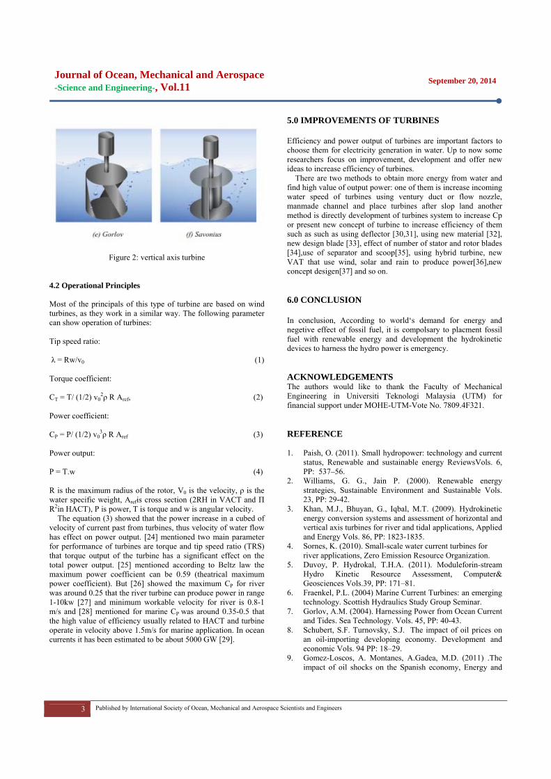
It is considerable that hydrokinetic turbine has a lot of similarities with wind turbine in terms of the physical principles of operation, electrical hardware, and variable speed capability for optimal energy extraction [20]. However, water is almost 800 times denser than air, therefore hydrokinetic turbines are more efficient than wind turbine even at low speed [21], [22]. 4.1 Turbines According to alignment of rotor axes with respect to the water flow, there are two main category of turbine to harness kinetic energy of water to generate electricity, horizontal axis (axial axis) and cross flow (vertical axis turbine)[3-7] as shown in figure 1 and 2. Which both types depend on condition and size can be used for river or marine. Inclined axis more used in river application and other axial-flow turbines are mainly used for the extraction of ocean energy. In the vertical axis domain, Darrieus turbines are the most prominent options that use of H-Darrieus or Squirrel-cage Darrieus (straight bladed) turbine is very common.

There is no consensus yet on whether horizontal-axis or vertical axis will be the best option for using current water energy but the vertical axis turbine appears to be advantageous to the horizontal axis turbine in several aspects [23].

Figure 1: horizontal axis turbine


September 20, 2014


Figure 2: vertical axis turbine 4.2 Operational Principles Most of the principals of this type of turbine are based on wind turbines, as they work in a similar way. The following parameter can show operation of turbines: Tip speed ratio: λ = Rw/v0 (1) Torque coefficient: CT = T/ (1/2) v0

2ρ R Aref, (2) Power coefficient: CP = P/ (1/2) v0

3ρ R Aref (3) Power output: P = T.w (4) R is the maximum radius of the rotor, V0 is the velocity, ρ is the water specific weight, Arefis cross section (2RH in VACT and П R2in HACT), P is power, T is torque and w is angular velocity.

The equation (3) showed that the power increase in a cubed of velocity of current past from turbines, thus velocity of water flow has effect on power output. [24] mentioned two main parameter for performance of turbines are torque and tip speed ratio (TRS) that torque output of the turbine has a significant effect on the total power output. [25] mentioned according to Beltz law the maximum power coefficient can be 0.59 (theatrical maximum power coefficient). But [26] showed the maximum CP for river was around 0.25 that the river turbine can produce power in range 1-10kw [27] and minimum workable velocity for river is 0.8-1 m/s and [28] mentioned for marine CP was around 0.35-0.5 that the high value of efficiency usually related to HACT and turbine operate in velocity above 1.5m/s for marine application. In ocean currents it has been estimated to be about 5000 GW [29].

5.0 IMPROVEMENTS OF TURBINES

Efficiency and power output of turbines are important factors to choose them for electricity generation in water. Up to now some researchers focus on improvement, development and offer new ideas to increase efficiency of turbines.

There are two methods to obtain more energy from water and find high value of output power: one of them is increase incoming water speed of turbines using ventury duct or flow nozzle, manmade channel and place turbines after slop land another method is directly development of turbines system to increase Cp or present new concept of turbine to increase efficiency of them such as such as using deflector [30,31], using new material [32], new design blade [33], effect of number of stator and rotor blades [34],use of separator and scoop[35], using hybrid turbine, new VAT that use wind, solar and rain to produce power[36],new concept desigen[37] and so on. 6.0 CONCLUSION

In conclusion, According to world‘s demand for energy and negetive effect of fossil fuel, it is compolsary to placment fossil fuel with renewable energy and development the hydrokinetic devices to harness the hydro power is emergency. ACKNOWLEDGEMENTS The authors would like to thank the Faculty of Mechanical Engineering in Universiti Teknologi Malaysia (UTM) for financial support under MOHE-UTM-Vote No. 7809.4F321. REFERENCE 1. Paish, O. (2011). Small hydropower: technology and current

status, Renewable and sustainable energy ReviewsVols. 6, PP: 537–56.

2. Williams, G. G., Jain P. (2000). Renewable energy strategies, Sustainable Environment and Sustainable Vols. 23, PP: 29-42.

3. Khan, M.J., Bhuyan, G., Iqbal, M.T. (2009). Hydrokinetic energy conversion systems and assessment of horizontal and vertical axis turbines for river and tidal applications, Applied and Energy Vols. 86, PP: 1823-1835.

4. Sornes, K. (2010). Small-scale water current turbines for river applications, Zero Emission Resource Organization.

5. Duvoy, P. Hydrokal, T.H.A. (2011). Moduleforin-stream Hydro Kinetic Resource Assessment, Computer& Geosciences Vols.39, PP: 171–81.

6. Fraenkel, P.L. (2004) Marine Current Turbines: an emerging technology. Scottish Hydraulics Study Group Seminar.

7. Gorlov, A.M. (2004). Harnessing Power from Ocean Current and Tides. Sea Technology. Vols. 45, PP: 40-43.

8. Schubert, S.F. Turnovsky, S.J. The impact of oil prices on an oil-importing developing economy. Development and economic Vols. 94 PP: 18–29.

9. Gomez-Loscos, A. Montanes, A.Gadea, M.D. (2011) .The impact of oil shocks on the Spanish economy, Energy and


September 20, 2014


economy. Vols. 33, PP:1070–81. 10. Ali Ahmed, H.J. Wadud, I.K.M.M. (2011). Role of oil price

shocks on macroeconomic activities: an SVAR approach to the Malaysian economy and monetary responses. J. Energy and policy. Vola.39 , PP:8062–9.

11. Zevenhoven, R.Beyene, A. (2011).the relative contribution of waste heat from power plants to global warming, Energy Vols. 36,PP: 3754–62.

12. Harris, D. (2011). Monitoring global warming, J. Energy and Environment Vols. 22, PP: 929–37.

13. Peters, G.P. Aamaas, B.T. Lund, M. Solli, C. Fuglestvedt,J.S. (2011). Alternative global warming metrics in life cycle assessment: a case study with existing transportation data, Environment and science and technology Vols.45, PP:8633–41.

14. Analyses and Projections, U.S. Energy Information Administration, http://www.eia.doe.gov/analysis/; 2011.

15. Department of Statistics, Malaysia. Electricity. Available at: /http://www.statistics.gov.my/portal/download_Economics/download.php.2012.

16. Department of Statistics, Malaysia. Mining, Manufacturing and electricity. Available at: /http://www.statistics.gov.my/portal/download_Buletin_Bulanan/download.php?file=BPBM/2012/JAN/08_Mining.pdfS.2012.

17. Chong, H.Y. Lam, W.H. Ocean renewable energy in Malaysia: The potential of the Straits of Malacca, 2013.

18. Ministry of Energy, Green Technology and Water, Malaysia. National Renewable Energy Policy & Action Plan. Kuala Lumpur: KeTTHA; 2009.

19. Vermaak, H. J. Kusakanan, K. Koko, S.P. (2014) .Status of micro-hydrokinetic river technology in rural applications. Renewable and sustainable energy Reviews, vols. 29, pp. 625–633.

20. Zhou, H. (2012). Maximum power point tracking control of hydrokinetic turbine and low-speed high-thrust permanent magnet generator design [MSc thesis].Missouri University of Science and Technology.

21. Kuschke, M. Strunz, K. (2011). Modeling of tidal energy conversion systems for smart grid operation, In: IEEE Power and Energy Society General Meeting. (Detroit).

22. Yuen, K. Thomas, K. Grabbe, M. Deglaire, P. Bouquerel, M. Österberg, D. (2009) .Matching a permanent magnet synchronous generator to a fixed pitch vertical axis turbine for marine current energy conversion, Ocean engineering IEE, vol. 34.

23. Eriksson, S. Bernhoff, H. Leijon, M. (2006). Evaluation of different turbine concepts for wind power,Swedish Centre for Renewable Electric Energy Conversion, Division for Electricity and Lightning Research.

24. Gorban, A.N.Gorlov, A.M. Silantyev, V.M. (2001). Limits of the turbine efficiency for free fluid flow, Energy. Res. TechnologyASME,vol. 123, pp. 311–7, 2001.

25. Portnov, G.G. Palley, I.Z. (1998). Application of the Theory of naturally curved and twisted bars to designing Gorlov’s helical turbine, Mechanical Composite Material vol. 34, PP. 343–54.

26. Paraschivoiu, I. (2002). Wind turbine design: with emphasis on Darrieus concept, Canada: Poly technical Int Press.

27. Maitre, T. Achard. J.L. Antheaume, S. (2008). Hydraulic

Darrieus turbines efficiency for free fluid flow conditions versus power farms conditions, RenewableEneregy, vol. 33, pp. 2186–2198.

28. Han, S.H. Park, J.S. Lee, K.S. (2013). Park, W.S. Yi, J. H. Evaluation of vertical axis turbine characteristics for tidal current power plant based on in situ experiment, OceanEngineering vol. 65, pp. 83–89.

29. Ben Elghali, S.E. Balme,R.S.k. Benbouzid, M.E.H. Charpentier, J.F. Hauville, F.A.(2007). Simulation model for the evaluation of the electrical power potential harnessed by a marine current turbine in the Raz de Sein, .Ocean Engineering vol. 32, pp. 786–97.

30. Golecha, K. Eldho, T.I. Prabhu, S.V. (2011). Influence of the deflector plate on the performance of a modified Savoniuswater turbine, Applied Energy. Vols. 88 ,pp: 3207–17.

31. Golecha, K. Eldho, T.I. Prabhu, S.V. (2011). Investigation on the performance of a modified Savonius water turbine with single and two deflector plates.

32. Nicholls, R. L. (2008). Utilizing intelligent materials in the design of tidal turbine blades. Fluid and structure interaction research group. Southampton, UK: University of Southampton.

33. Zanette, J. Imbault, D. Tourabi, A. (2010). A design methodology for cross flow water turbines, J. Renewable energy. Vols. 35 pp: 997–1009.

34. Asim, T. Mishra, R. Ubbi, K. Zala,K. (2013). Computational Fluid Dynamics Based Optimal Design of Vertical Axis Marine Current Turbines.

35. [42] W.M.J. Batten, G.U. Batten, Potential for using the floating body structure to increase the efficiency of a free stream energy converter. 2011. pp. 2364–2371.

36. Chong, W.T. Fazlizan, A.Poh, S.C. Pan, K.C. Ping, H.W. (2012). Early development of an innovative building integrated wind, solar and rain water harvester for urban high rise application, Energy and building. Vols. 47 pp: 201-207.

37. Lam, W. H. Bhatia, A. (2013). Folding tidal turbine as an innovative concept toward the new era of turbines, Renewable and SustainableEnergy Reviews, Vols.28,pp: 463-473.


September 20, 2014


CO2 Emission of Marine Transports in Batam - Singapore

M.Rashidi,b and Jaswar Koto,a,b,*

a)Ocean and Aerospace Research Institute, Indonesia b)Mechanical Engineering Faculty, Universiti Teknologi Malaysia (UTM), 81310, Johor, Malaysia *Corresponding author: [email protected] Paper History Received: 5-September-2014 Received in revised form: 10-September -2013 Accepted: 18-September -2014 ABSTRACT Global warming and air pollution have become one of the important issues to the entire world community. Exhaust emissions from ships has been contributing to the health problems and environmental damage. This study focuses on the Strait of Malacca area because it is one of the world’s most congested straits used for international shipping where located on the border among three countries of Indonesia, Malaysia and Singapore. This study will predict CO2 emission from the marine transport. This is accomplished by developed a ship database in the Straits of Malacca by using the data which obtained from Automatic Identification System (AIS). From the database, MEET methodology is used to estimate the CO2 emission from ships. KEY WORDS: Automatic Identification System, CO2, Carbon Dioxide, Emission, Distribution. NOMENCLATURE IMO International Maritime Organization

Carbon Dioxide GHG Green House Gas GT Gross Tonnage AIS Automatic Identification System

1.0 INTRODUCTION

The Strait of Malacca is one of the most important shipping channels in the world which is connecting the Indian Ocean with the South China Sea and the Pacific Ocean. At approximately 805 kilometers long, the Strait of Malacca is the longest Strait in the world used for international navigation (Wikipedia, 2013). The Strait of Malacca is a narrow stretch of water lying between the east coast of Sumatra Island in Indonesia and the west coast of Peninsular Malaysia, and is linked to Singapore at its southeast end. The Strait of Malacca varies in width from 200 miles to 11 miles with irregular depths from over 70 to less than 10 meters (SJICL, 1998).

The Strait of Malacca remains as one of the world most congested straits used for international shipping. From the study by Jaswar (2013), it shows that daily 1500 vessels approximately pass through the Strait of Malacca which is 42 percent was under Singaporean flag. These consist of a wide spectrum of different types of vessels with 32 percent of Liquid bulk and 11 percent of container ships.

With this number of ship, it will leave environmental impact such as Greenhouse gas emission. CO2 emissions from shipping is estimated to be 4 to 5 percent of the global total, and estimated by the International Maritime Organization (IMO) to rise by as much as 72 percent by 2020 if no action is taken (Vidal, 2007). IMO (2009) study of greenhouse gas (GHG) shows total exhaust emission from shipping from 1990 to 2007 and can see that there are increases of exhaust emission every year. This paper discusses the prediction of CO2 emission by marine transport. 2.0 AUTOMATIC IDENTIFICATION SYSTEM

Automatic Identification System (AIS) firstly has been used to comply with safety and security regulations, functioning as


September 20, 2014


collision avoidance, vessel traffic services, maritime security, aids to navigation, search and rescue and accident investigation. The AIS is meant to be used primarily as a means of lookout and to determine the risk of collision rather than as an automatic collision avoidance system, in accordance with the International Regulations for Preventing Collisions at Sea (IMO, 1998).

Primary data of ships which obtained from an AIS receiver in the study are MMSI of the ship, IMO number, receive time, position of the ship (longitude and latitude), speed of ground (SOG) and COG. These all the data obtained from an AIS receiver installed in Marine Technology Laboratory (Marine Technology Center (MTC)), Faculty of Mechanical Engineering, UniversitiTeknologi Malaysia (UTM). Information of ships based on AIS is not complete to use as the basis for calculation. AIS only provides several initial data such as MMSI, IMO number, position of ships (longitude and latitude), Speed Over Ground (SOG), Centre of Gratify (COG) and true heading of the ship. Gross Tonnage (GT) data for calculation of emission rate as explained by Trozzi C. (2010) is obtained from other references such as marinetraffic.com, maritime-connector.com, equasis.org, vesseltracker.com and Equasis.org. The combination of all the data will make a complete database that can be used for the calculation. 3.0 CARBON DIOXIDE

Carbon dioxide (CO2) is a colorless, odorless, non-flammable gas that is a product of cellular respiration and burning of fossil fuels. It has a molecular weight of 44.01g/Mol (NIOSH 1976). Although it is typically present as a gas, carbon dioxide also can be a solid form as dry ice and liquefied, depending on temperature and pressure (Nelson 2000). Carbon dioxide is not only a gas which affects the heat flow to and from the atmosphere of the earth, but is also a serious pollutant in its own right (Robertson, 2006). The concentration of this gas in the atmosphere is not known to have risen above 320 ppm over the last 40,000 years (Neftal et al, 1982).

Evidence demonstrates this to be the case for the past 420,000 years (Petit et al, 1999). Several researches suggest that carbon dioxides also give effect to the Physiological. Although the safe working level of carbon dioxide is presently set at 5000 ppm for an 8 h day 40 h working week, no human ever endures such a level of carbon dioxide in the atmosphere for 24 h a day, 365 days a year, for an entire lifetime nor has any human ever bred offspring under these conditions. This includes workers in breweries and the greenhouse industry, where the concentration of carbon dioxide in the atmosphere either commonly reaches or is set at a maximum of 900 ppm (Robertson, 2006).

Methodologies for estimating air pollutant emissions from ships, in port environment and in navigation have been developed for one of the framework of the MEET project (Methodologies for estimating air pollutant emissions from transport). The methodology has been developed under the transport RTD program of the European Commission fourth framework program (EEA). MEET Methodology was adopted by Trozzi et.al (1998),

Trozzi et.al (1999) and Pitana et.al (2010) for estimating emissions from ships.

Methodologies for estimating air pollutant emissions from ships used to estimate of consumption and emissions based on present day statistics of ship traffic (Trozzi et al, 1998). The methodology is used by consider twelve ship class of ship with a gross tonnage above 100 GT. The data need such as emission factors, fuel consumption of ship, type of engine, etc. Fuel consumption of any type of ship are obtained from a linear regression analysis of fuel consumption to gross tonnage as shown in the table below.

Table 1: Average consumption at full power versus gross tonnage

Ship types Consumption at full power (t/day) as function of gross tonnage

Solid Bulk (SB) Cjk = 20.1860 + 0.00049 × GT Liquid Bulk /Tanker (LB) Cjk = 14.6850 + 0.00079 × GT General Cargo (GC) Cjk = 9.8197 + 0.00143 × GT Container (CO) Cjk = 8.0552 + 0.00235 × GT Ro-Ro Cargo (PC) Cjk = 12.8340 + 0.00156 × GT Passenger (PA) Cjk = 16.9040 + 0.00198 × GT High Speed Ferry (HS) Cjk = 39.4830 + 0.00972 × GT Inland Cargo (IC) Cjk = 9.8197 + 0.00143 × GT Sail Ship (SS) Cjk = 0.4268 + 0.00100 × GT Tugs (TU) Cjk = 5.6511 + 0.01048 × GT Fishing (FI) Cjk = 1.9387 + 0.00448 × GT Other Ships (OT) Cjk = 9.7126 + 0.00091 × GT

Table 2: Emission factors (kg/ton of fuel)

Phases Engine types CO2 Cruising Steam turbines - BFO 3200

Steam turbines - MDO 3200 High speed diesel engines 3200 Medium speed diesel engines 3200 Slow speed diesel engines 3200 Gas turbines 3200 Pleasure – Inboard diesel 3200 Pleasure – Inboard gasoline 3000 Outboard gasoline engines 3000

Manoeuvring Steam turbines – BFO 3200 Steam turbines – MDO 3200 High speed diesel engines 3200 Medium speed diesel engines 3200 Slow speed diesel engines 3200 Gas turbines 3200 Pleasure – Inboard diesel 3200 Pleasure – Inboard gasoline 3000 Outboard gasoline engines 3000

Hotelling Steam turbines – BFO 3200 Steam turbines – MDO 3200 High speed diesel engines 3200


September 20, 2014


Medium speed diesel engine 3200 Slow speed diesel engines 3200 Gas turbines 3200 Pleasure – Inboard diesel neg. Pleasure – Inboard gasoline neg. Outboard gasoline engines neg.

Tanker load. /off-load. 3200

Table 3: Fraction of maximum fuel consumption in different mode

Mode Fraction

Cruising 0.8

Manoeuvring 0.4

Hotelling default 0.2

passenger 0.32

liquid bulk 0.2

other 0.12

Tug: ship assistance 0.2

moderate activity 0.5

under tow 0.8 To calculate the emission rate of each vessel based on the

assumption of the above tables, Trozzi et al (1998) using the following equation:

(1)

With ….. (2)

Where, i pollutant j fuel (see table ) k ship class for use in consumption classification (see table ) l engines type class for use in emission factors

characterization (see table ) s reference reduction scenario (low, medium, high) Ei total emissions of pollutant i Eijklm total emissions of pollutant i from use of fuel j on ship

class k with engines type l in mode operation m Sjkm (GT) daily consumption of fuel j in ship class k as a

function of gross tonnage tjklm days in navigation of ships of class k with engines type

l using fuel j in mode operational m Fijlm average emission factors of pollutant i from fuel j in

engines type l in mode m

Table 4: Fuels classification Code Name RO Residual oils DO Distillate oil DF Diesel fuel GF Gasoline fuel

Table 5: Engines type class

Code Name SE Steam turbines HS High speed motor engines MS Medium speed motor engines SS Slow speed motor engines

IP Inboard engines - pleasure craft(only for detailed methodology)

OP Outboard engines(only for detailed methodology)

TO Tanker loading and off-loading(only for detailed methodology)

Table 6: Ship type class

Code Name SB Solid Bulk LB Liquid Bulk GC General Cargo CO Container PC Ro-Ro Cargo PA Passenger HS High speed ferries IC Inland Cargo SS Sail ships TU Tugs FI Fishing OT Other Calculation of emission and the concentration are performed by

using programming. The high number of calculation and output of the calculation becomes an issue when it calculated by manually. The programming which used for this step is Microsoft Visual Studio 2010. 4.0 CASE STUDY

Calculation of emission is estimated for every ship which is recorded by AIS on September 2, 2011 at 7.00am - 8.00am. There were 813 total number of ships are counted. Calculations of emission based on the standard European (MEET) methodology which adopted by Trozzi et.al (1998). The result is presented in percentage. The calculations by considering several factors are:

i. Gross Tonnage (GT) ii. Type of ship

iii. Mode operation of ship

Journal o-Science an

8 P

iv. Fuel v. Main

of Ocean, Mnd Engineerin

Published by Interna

type n engine and au

Figure 1

Figure 2: M

Mechanical ng-, Vol.11

ational Society of O

uxiliary engine p

: Marine Track

Marine Emissio

and Aeros

Ocean, Mechanical a

power

king

on

space

and Aerospace Scie

C

S

L

GC

PP

HTFOU

TTsh

F

SMC

Ro

H

entists and Engineer

Ta

Code Ty

SB Solid

LB LiquidBulk

GC GenerCargo

CO Conta

PC Ro-RoCargo

PA Passen

HS Highferries

TU TugsFI FishinOT OtherUnknown

Total Number oTotal correspohip

Figure 4: P

Flag

Singapore Malaysia China People’s

Contain38%

o‐Ro Cargo0%

Passenger0%

igh speed ferries0%

Tugs5%

rs

Figure 3: C

able 7: CO2 emi

ype Numbof Sh

Bulk 49d

372ral o 51ainer 124o o 3 nger 12speed

s 1 138

ng 1 62360

f Ship 117ondent

813

Percentage of C

Table 8: CO2

Number of Ship

344 28

s 8

ner

Fishing0%

O

CO2 Perc

Se

CO2 Emission

ission by type o

ber hip

CO2 g/tonfuel persecond

729.93

2 4549.1

305.844 4220.9

28.23345.098

3.257 8 524.52

8.548 677.46

0 Unknow

73 11092.

3

CO2 emission by

2 emission by flCO2 g/ton oper-second

2513.719 183.373 151.466

Solid Bulk7%

Other6%

centage by s

eptember 20, 20

of ship

n of r-d

CO2Percent

by shiType

0 6.580

25 41.00

3 2.75772 38.05

0.255 0.407

0.0296 4.728

0.0778 6.107

wn Unknow

999 100.0

%

y types of ship

lag of fuel) CO2

by Fl221.61.3

k

Liquid Bulk41%

General Cargo3%

ship Type

014

age ip e 0%

09%

7% 1%

% 7%

9% 8% 7% 7% wn

000

% lag

2.66% 65% 37%

vie

Journal o-Science an

9 P

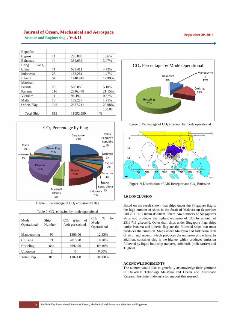
Republic Cyprus Bahamas Hong KongChina Indonesia Liberia Marshall Islands Panama Vietnam Malta Others Flag

Total Ship

Figu

Tab

Mode Operational

Manoeuvring Cruising Hotteling Unknown Total Ship

Panam21%

etnam1%

Malta2%

of Ocean, Mnd Engineerin

Published by Interna

11 14

g, 21 28 54

29 110 11 13 142

813

ure 5: Percentag

ble 9: CO2 emis

Ship Number

96 71 644

2 813

Marshall Islands5%

ma%

Others Flag21%

CO2 Perce

Mechanical ng-, Vol.11

ational Society of O

206.808 384.639

523.411 163.281 1440.845

566.050 2346.47896.492 189.227 2327.211

11092.99

ge of CO2 emiss

ssion by mode o

CO2 g/ton fuel) per secon

1366.06 2015.78 7692.95

0 11074.8

Singapore23%

lIberia13%

entage by Fl

and Aeros

Ocean, Mechanical a

13

41

5 1

58 2

01

1 2

99 1

%

sion by flag

operational

of nd

CO2 %Mode Operation

12.3318.2069.460.00

100.0

e

M

CPeRe

Ba

HoKong

5Indonesia1%

lag

space

and Aerospace Scie

1.86% 3.47%

4.72% 1.47% 12.99%

5.10% 21.15% 0.87% 1.71% 20.98% 100.00

% by

nal

3% 0% 6% % 0%

4

Bth2sh2upoafoT

ATtoR

Malaysia2%

China eoples's epublic1%

Cyprus2%

ahamas3%

ong g, China5%

entists and Engineer

Figure 6: Per

Figure 7: Di

4.0 CONCLUSI

Based on the rehe high numbe

2nd 2011 at 7.0hips and produ

2513.718 g/secounder Panama aproduces the emof sixth and sevaddition, containollowed by liqu

Tugboat.

ACKNOWLEDThe authors wouo Universiti T

Research Institu

Ho

CO2 Pe

rs

rcentage of CO

istribution of A

ION

esult shown thar of ships in th0am-08.00am. uces the highesond. Other thanand Liberia flag

mission. Ships uventh which proner ship is theuid bulk ship (ta

DGEMENTS uld like to grat

Teknologi Malaute, Indonesia fo

otteling70%

Unk0

ercentage by

Se

O2 emission by m

AIS Receptor an

at ships under thhe Strait of MaThere 344 numst emission of n ships under Sg are the followunder Malaysiaoduces the emie highest whichanker), solid bu

tefully acknowlaysia and Oceor support this r

known0%

y Mode Ope

eptember 20, 20

mode operation

nd CO2 Emissio

he Singapore flalacca on Septembers of Singap

CO2 by amouSingapore flag, wed ships that

a and Indonesiassion at the tim

h produces emiulk (bulk carrier

ledge their gratean and Aeroresearch.

Manoeuvg

12%

Cruising18%

erational

014

nal

n

flag is ember pore's unt of

ships most

a rank me. In ission r) and

titude space

vrin


September 20, 2014


REFERENCES

1. IMO (International Maritime Organization). 1998. IMO Resolution MSC.74 (69). “Recommendation on Performance Standards for A Universal Shipborne Automatic Identification System (AIS)”.

2. IMO. 2009. Second IMO GHG Study 2009. International Maritime Organization (IMO), 4 Albert Embankments, London SE1 7SR Protection Agency Research Triangle Park, North Carolina 27711

3. Jaswar, M.Rashidi, A.Maimun, 2013, “Tracking of ships navigation in the Strait of Malacca using automatic identification system”, Developments in Maritime Transportation and Exploitation of Sea Resources, Taylor & Francis Group, London, ISBN 978-1-138-00124-4

4. National Institute for Occupational Safety and Health (NIOSH). 1976. Criteria for a Recommended Standard, Occupational Exposure to Carbon Dioxide. August 1976.

5. Neftal, A., Oeschger, H., Schwander, J., Steuffer, B. and Zumbrunn, R., 1982. Ice core sample measurement gives atmospheric CO2 content over the past 40,000 yr. Nature, 1982, 295, 220–223.

6. Nelson, L. 2000. Carbon Dioxide Poisoning. Emerg. Medicine 32(5):36-38. Summary of physiological effects and toxicology of CO2 on humans.

7. Robertson, D. S. 2006. Health effects of increase in concentration of carbon dioxide in the atmosphere. Current Science, Vol. 90, No. 12, 25 June 2006.

8. SJICL, 1998, Navigation Safety in the Strait of Malacca, Singapore Journal of International & Comparative Law, pp.468–485.

9. Trozzi C. 2010. Update of Emission Estimate Methodology for Maritime Navigation, Techne Consulting report ETC.EF.10 DD, May 2010.

10. Vidal, J. 2007 "CO2 Output from Shipping Twice As Much As Airlines". TheGuardian (London).


September 20, 2014


A Chebyshev Polynomial on Torque and Thrust Coefficients of Mathematical Propeller Properties for a LNG Manoeuvring

Simulation

Sunarsih,a, Agoes Priyanto,a, b,*, Mohd. Zamani,a, and Nur Izzudin,a

a) Faculty of Mechanical Engineering, Unversiti Teknologi Malaysia, UTM Skudai 81300, Johor Bahru, Malaysia b)Marine Technology Centre, Unversiti Teknologi Malaysia, UTM Skudai 81300, Johor Bahru, Malaysia *Corresponding author: [email protected] Paper History Received: 15-September-2014 Received in revised form: 17- September -2013 Accepted: 19- September -2014 ABSTRACT The estimated torque and thrust coefficients in four quadrants of marine propeller in a LNG manoeuvre control system is essential for the total performance of the vessel. A Chebyshev n-order polynomial that approximated a continuous function over the interval advance speed J [-1, 1] to calculate the torque and thrust coefficients as well as the shaft speed, is utilized to get the propeller properties. The Dynamical modeling and simulation of the marine propeller across the four quadrants are schemed and applied to the marine propeller B-4.58. The results are compared with both open water experiments and open water numerical tests using ANSYS-Fluent. The comparisons show that the chebyshev polynomial agreed well with both experiments and numerical tests and deduce that the polynomial provides a new practically approach estimation on torque and thrust coefficients in four quadrants of marine propeller for the vessel operations. Then the polynomial coefficients from Chebyshev n-order polynomial were used to express the mathematical model for the propeller thrust and torque characteristics and applied in the manoeuvring simulation programming. KEY WORDS: Chebyshev Polynomial, Propeller Properties, Ansys Fluent, Manoeuvring Simulation.

1.0 INTRODUCTION

There exist some notable problems regarding ship manoeuvring which has been observed to change significantly according to canal regions. The ship-bank effect in shallow water becomes significant when the ship travels close to the bank. A large vessel experiences lateral force and turning moment by asymmetric flow around the ship’s hull due to the presence of the bank in a very narrow waterway [15], [16], [17]. This phenomenon may even become critical [18)] when as it causes difficulties in controlling the ship along its intended course this in turn increases the possibility of grounding or collision. In November 2007 at Suez Canal, the same type of ship had the same incident when the ship was turning back to the starboard. This point can be illustrated by two pilots and the master failed to regain control of the LNG vessel following a manoeuvre at reduced-speed in a canal. The vessel was proceeding South with new pilots and approached close to the Eastern bank, while navigating the canal bend opposite a Lake. The vessel appeared to become course-unstable after successive 35 degree helm operations to port and starboard, during which the vessel struck the Eastern bank 15 minutes after the start of the manoeuvre and grounded on the Western bank after a further 4 minutes. [18] have proposed valuable information on potential remedial actions for LNG tanker manoeuvre in the canal, such as a combination work between fitting two pairs of fins and increasing the effectiveness of the existing rudder at low ship speed and developed the manoeuvring simulation by MATLAB Simulink to solve the problem.

The manoeuvring simulation solves the surge, sway, and yaw motions with respect to CoG of tanker. The mathematical model of external forces on the tanker composed of hydrodynamic hull, rudder force and propeller force as well as the hydrodynamic hull-banks interactions. In the simulation the mathematical model propeller force in X-direction were expressed by polynomial


September 20, 2014


coefficients order three from Kt-J, and Kq-J diagrams. The polynomial coefficients expression for the propeller thrust and torque characteristic were determined from the open water propeller tests.

Such a model in curve from is immediate and obvious, but it is not convenient to do mathematical analysis and simulation programming. Usually polynomial fitting form is adopted by ordinary polynomial. The principle weakness of ordinary polynomial fitting is that the fitting results from open water tests are not in common use. For different order n, in order keep higher fitting accuracy, it is necessary to use different set of polynomial coefficients and to refit new. Using ordinary polynomial fitting to meet different requirements, many set of coefficients must be prepared and it is convenient. If polynomial coefficients are kept invariant, only the order number is increased and decreased. The best way this problem is to use Chebyshev polynomial fitting. The thrust coefficient Kt, torque co

( ) )0(,/ 24 ≠= NNDTKt ρ (1)

( ) )0(,/ 25 ≠= NNDQKq ρ (2)

( ) )0(,/ ≠= NDNvJ p (3) where vp is the propeller velocity relative to water, T and Q are propeller thrust and torque respectively, D is propeller diameter. For a given propeller pitch to D ratio P/D, the relation T, Q and J are expressed as

( ),JKKt t= ( )JKKq q= (4)

On Kt-J diagram or Kq-J diagram stride across four quadrants generally and Kt, Kq and J stretch to infinite. When N and vp are not equal to zero at the same time they are defined as

( )( ) ( ),1// 22222' JKtNDvDTtK p +=+= ρ (5)

( )( ) ( )22223' 1// JKqNDvDQqK p +=+= ρ (6)

222' / NDvvJ pp += (7)

It can be seen that J=(-∞,∞) is mapped to J=(-1,1).

This paper will discuss Chebyshev polynomial and get results the polynomial coefficients of the propeller B4-58, disc square ratio A0/Ad =0.58, blade=4, wing type section and screw pitch ratio P/D=1. The results then were compared with both open water experiments and open water numerical tests using ANSYS-Fluent V.6. As an application, this method is applied in the mathematical model for propeller properties in Chebyshev polynomial and used to simulate manoeuvring of LNG tanker. 2.0 NUMERICAL ESTIMATION.

2.1. Chebyshev Polynomial Propellers are usually designed to produce thrust in one direction

and propel the ship ahead. Nonetheless, the ship sometimes has to produce thrust in the reverse direction to propel the ship backward. Furthermore, the propeller maybe uses to decelerate the ship by running in the opposite direction of the advance speed. Addressing these issues, the four quadrants of propeller operation provide discretion in serving such functions. The characteristics, as presented in Table 1, are determined by the positive or negative operation of ship speed (Vs) and the propeller rotation (N).

Table 1: Propeller quadrants of operation.

1 2 3 4 N ≥ 0 < 0 < 0 ≥ 0 Vs ≥ 0 ≥ 0 < 0 < 0

whereVp is advance speed of the propeller relative to water approximated using the following expression: Vp= (1-w) Vs (8)

The standard (first quadrant) and four-quadrant propeller characteristics used to describe the thrust and torque in steady-state conditions. However, the degradation of the propeller performance will occur if the propeller is subjected to cross-flow or is not deeply submerged by employing thrust and torque loss functions. In that case, additional measurements of the cross flow velocity and the propeller submergence are necessitated. The following Fig. 1 illustrates the four quadrants representing the four combinations of speed and thrust directions.

When the ship manoeuvres in steady state, the advance ratio J varies in a small range (J [0.6, 0.8]) while it significantly changes during the dynamic state and even can be negative in values [1] – [10]. Usually polynomial fitting form is adopted as follows:

( ) nn

n

j

jj xbxbbxbxg +++=∑=

=...10

0 (9)

Meanwhile a continuous function over the interval [-1, 1] can be expressed also approximately as n-th order of Chebyshev polynomial [5] written as:

∑ (10)

where T0(x)=1, T1(x)=x, T2(x)=2x2 – 1, T3(x)=4x3 – 3x, … while the general recursive formula for Tk(x) is given by:

Tk(x) = 2xTk-1(x)– Tk-2(x); k ≥ 2 (11)

The feature of the Chebyshev polynomial is that Tj (x) and Tk (x) are orthogonal to each other and the polynomial coefficients are independent of the order n. Furthermore, the fitting error is small and the fitting result with finite order n is the best approximation within the meaning of minimum square error. It is convenient to change into ordinary polynomial a given Chebyshev polynomial expression.


September 20, 2014


Figure 1: Four quadrants of ship speed and propeller operations.

For a given screw-pitch ratio H/D, the approximation of the propeller thrust coefficient Kt and torque coefficient Kq properties across four quadrants with such Chebyshev polynomial (n=8) are expressed by: ′ ′ ′ ′ ′ (12)

′ ′ ′ ′ ′ (13)

Substituting Chebyshev polynomial a0 – an in Table 2 into

extending T0 – Tn, by definition. Moreover the ordinary polynomials are expressed by: ′ ′ (14)

′ (15)

The ordinary polynomial and its coefficients b0 – bn can be obtained as shown in Table 3 by using Eqs.(12) – (15). Table 2: Chebyshev Polynomial Coefficients of Thrust and Torque Properties.

a Kt' Kq' n>0 n<0 n>0 n<0

a0 0.3888 -0.2641 0.05315 -0.04467 a1 -0.2338 -0.2274 -0.03093 -0.03423 a2 -0.1664 0.1254 -0.0226 0.0249 a3 -0.02003 -0.02646 -0.00406 -0.00458 a4 0.00134 -0.00152 0.000832 -0.00154 a5 0.05241 0.04883 0.006672 0.007792 a6 -0.02842 0.02704 -0.00184 0.004162 a7 0.02029 0.01888 0.004078 0.004694 a8 0.01766 -0.00632 0.002371 -0.001650

Table 3: Ordinary Polynomial Coefficients of Thrust and Torque Properties

b Kt Kq n>0 n<0 n>0 n<0

b0 0.04924 -0.04312 0.1944 -0.13205 b1 0.03224 0.03609 0.21042 0.20466 b2 -0.02510 0.027739 -0.10317 0.077748 b3 0.00118 0.001799 0.004326 0.005715 b4 0.00009 -0.00041 -0.00031 0.000352 b5 0.00452 0.005294 0.033132 0.030868 b6 0.05450 -0.00696 0.025768 -0.02452 b7 0.00389 0.00431 0.020288 0.018878 b8 0.01766 -0.0006 -0.01577 0.005644

The LNG’s propeller has been taken to describe the method of calculating the alternatives properties, Chebyshev polynomial with n=8 were used. By calculation, we select screw pitch ratio P/D=1.0. Substituting into Eqs(12) – (15) the resulting expressions for interpolation for thrust coefficient and torque coefficients are plotted in Figs.(2) – (3). 2.2. Computational fluid dynamic (CFD). The computational fluid dynamics, as known as the CFD has become a practical tool in the simulation of hydrodynamics of marine devices, especially propeller [11] – [14]. A CFD study on the propeller open water test using the stationary domain length of about 6-7 times the propeller diameter to simulate the flow source and sink was conducted. The rotational domain which was close proximity to the propeller, could give a good simulation for the rotating region of fluid adaption surrounding the propeller. It adopted the multiple reference frame method, and the bigger rotating part was selected and it would produce more accurate results. A four bladed propeller B4-58 screw pitch ratio P/D=1.0 was used in the propeller properties estimation. The following assumptions or approach are implemented, namely the fluid domain numerically modelled via a finite volume method based


September 20, 2014


on the Reynold-Average Navier Stokes (RANS) equations, and the accuracy for applicability of first quadrant steady flow as shown in Fig. 1 were compared with the Chebyshev polynomial and the experimental results

In Cartesian tensor form the general RANS equations for continuity fluid can be written as:

( ) 0=∂

∂+

∂∂

xu

tiρρ

(16)

The momentum equation becomes: ( ) ( ) ( )''

32

jiji

iij

i

j

j

i

jij

jii uuxx

uxu

xu

xxp

xuu

tu ρδμ

ρρ−

∂∂

+⎥⎥⎦

⎤

⎢⎢⎣

⎡⎟⎟⎠

⎞⎜⎜⎝

⎛

∂∂

−∂

∂+

∂∂

∂∂

+∂∂

−=∂

∂+

∂∂

(17)

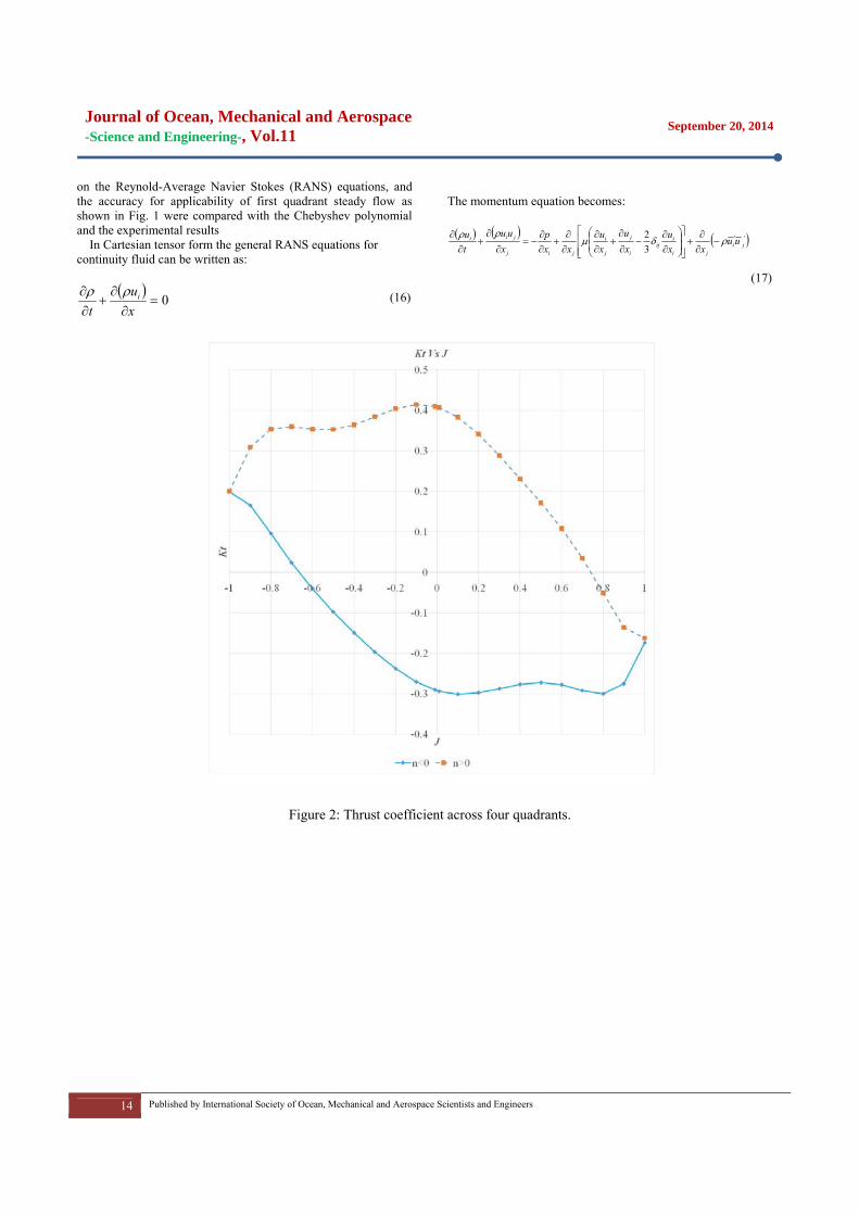
Figure 2: Thrust coefficient across four quadrants.


September 20, 2014


Figure 3. Torque coefficient across four quadrants. where δij in the Eq. (17) is the Kronecker delta, ′ ′ are the unknown Reynolds stresses that have to be modelled to close the momentum equation. With Boussinesq’s eddy-viscosity assumption and two transport equations for solving a turbulence velocity and turbulence time scale (turbulence modelling), RANS equations are closed. The commercial software Ansys Fluent applied a cell-centred finite volume method, and the velocity in the RANS equations in Eqs. (16) and (17) are solved in both moving reference frame for the steady calculation and the moving mesh for the transient calculation.

To model the turbulent flow, the steady turbulent model was applied in the ANSYS Fluent which is the standard k-epsilon model for the simulation. In the simulation, the propeller type B 4 – 58 was meshed as shown in Fig. 3. For the computational domain as shown in Fig. 4, the propeller blades were mounted on two finite long constant radius cylinders. The two types of cylinder domains, which have been developed, were stator domain and rotor domain. For the stator domain, the inlet flow is Lsi = 2D from blade, the outlet flow at Lso= 6D and the outer boundary is Ds=3.6D. While the rotor domain, the upstream remained Lbr=0.2D but the downstream was extended for cases open water test between Lfr= 0.4D and 0.7D, and the outer boundary is 1.4D. The turbulent model was simulated in the rotor domain by using the stator-rotor approaches such as the multiple reference frame (MRF) and the sliding mesh (SM) method. These

computational configurations are distinguished mainly by its size of rotational domain’s open water tests.


September 20, 2014


Figure 3: Propeller meshing.

Figure 4: Computational domain for the propeller.

An advance speed (ua) is used to initiate the inlet flow. Detailing the boundary conditions, velocity inlet was selected for stator inlet plane with intensity and viscosity ratio of 10 for the turbulent specification method. Pressure outlet is defined for the stator outlet with zero gauge pressure and similar turbulent specification as stator inlet. Convergence criterion was set up to 10-3 and solutions were converged within ranges of 200 to 1200 iterations as shown in Fig. 5, but not for very high J values. The open water curves is simulated by varying propeller rotation rate and fixed the value of advance speed. Convergence was set to 0.001 and iteration was converged to mere 600 in average open water condition. The rotating range between n=50 to 190 rpm were assigned and all boundaries inside this domain was specified as adjacent to cell zone, or the rotational fluid zone. 3.0 OPEN WATER TESTS.

The tests were carried out at the Marine Technology Centre, Universiti Teknologi Malaysia. The basin, 120 m long, 4 m wide and 2.5 m deep is equipped with a towing carriage that can reach a masximum speed of 4 m/s with a wave generator able to generate waves up to 0.4 m. We employed a three phase brushless motor in combination with a drive equipped with a built-in torque controller and a build-in shaft speed controller. In this way we

could choose to control the motor torque in order to obtain the desired motor torque or the shaft speed to obtain the desired ω. The motor was connected to the propeller shaft through a gear-box with ratio 1:1. The rig with motor, underwater housing, shaft and propeller was attached to the towing carriage in order to move the propeller through the water. The tests were performed on a fixed pitch propeller B4-58.

Figure 5: Open Water tests.

The shaft speed was measured on the motor shaft with a

tachometer dynamo. The thrust and torque were measured with an inductive transducer and a strain gauge transducer placed on the propeller shaft, respectively. The measurement of the motor torque was furnished by the motor drive. A picture of the propeller system is presented in Fig. 5. 4.0 RESULTS AND DISCUSSION.

In this section, it isn’t difficult to get an ordinary propeller atlas for the first quadrant. If alternatives properties with higher accuracy can be compared and found on the first quadrant by using other methods, it will be significant.

As an application this method is used to calculate LNG’s propeller’s alternative properties in Chebeyshev polynomial form providing in preceding section. Then they are used in comparison with calculation results of LNG’s propeller from Ansys FLUENT and Open Water tests. The model lays a foundation for LNG manoeuvering simulation. CFD of Ansys FLUENT and open water experiments practice shows that the results are very close to the practical data, as shown in Figs. 5 and 6, therefore are effective.

The Figs 6 and 7 displays the thrust and torque coefficients which decrease simultaneously with respect to the increase of advance ratio J values. A slight difference appears at both end points of comparison between the Chebyshev polysnomial and the experiment result. At the point of J = 0.4, the characteristic of the trust and torques coefficients are approaching similarly which values to 0.20 for Kt and 0.285 for 10Kq. However, the trend is quite lower for the estimation generated from the ANSYS Fluent. The results reveal that the torque coefficients generated from the Chebyshev expression for the inside domain have a fairly similar trend and values with the experimental result and also agreed well with the previous CFD study which adopted the multiple reference frame (MRF) method, that the bigger rotating part (Lr) is used and will produce more accurate results.


September 20, 2014


Figure 6: Comparison results for thrust coefficients.

Figure 7: Comparison results for torque coefficients.

5.0 LNG’S MANOEUVRING SIMULATION.

The mathematical model can be described by the Eqs. (18) – (20), using the coordinate system in Figure 8. As shown in Figure 7, (U) is the actual ship velocity that can be decomposed in an advance velocity (u) and a transversal velocity (v). The LNG ship has also a rotation velocity (r) with respect to the z-axis. This axis is normal to the XY plane and passes through the LNG ship centre of gravity (C.G). (β) is the angle between U and the x-axis and it is called drift angle. (ψ) is the LNG ship heading angle and (δ) is the rudder angle. X , Y and N represents the hydrodynamic force and moment acting on the mid ship of hull.

( )rvumX −= & (18)

( )ruvmY += & (19)

rIN zz &= (20)

Eqs. (18), (19), and (20) correspond to the surge, sway, and yaw motions, respectively. m is the mass of the ship, zzI is the moment of inertia with respect to the z-axis. u , v , and r are the surge, sway, and yaw velocities and u& , v& , and r& are the surge, sway, and yaw accelerations, respectively. X and Y represent the forces acting in the X and Y directions whilst N is the moment with respect to the z-axis. These forces and moment can be described by separating them into the following components:

Figure 8: Comparison results for torque coefficients.

RPH XXXX ++= (21)

BKRPH YYYYY +++= (22)

BKRPH NNNNN +++= (23)

Where: the subscripts H, P, R and BK refer to hull, propeller, rudder and bank effect, respectively. Eqs. (4), (5) and (6) follow to the concept given by the Mathematical Modelling Group (MMG) of Japan [Ogawa, A and Kansai, H , 1987]. The forces and moments acting on the hull can be approximated by the following polynomials of 'v and r′ by the following expressions

[ ] TMrrvvvruH RULrXvXrvXuXULX '21

21 222222 ρρ +′′+′′+′′′+′′= &&

(24)

⎥⎥⎦

⎤

⎢⎢⎣

⎡

′′+′′′+′′′

+′′+′′+′′+′′+′′=

322

322

21

rYrvYrvY

vYrYvYrYvYULY

rrrvrrvvr

vvvrvrvH

&& &&ρ

(25)

⎥⎥⎦

⎤

⎢⎢⎣

⎡

′′+′′′+′′′+′′

+′′+′′+′′+′= 3223

2321

rNrvNrvNvN

rNvNrNvNULN

rrrvrrvvrvvv

rvrvH

&& &&ρ

(26)

0.000.050.100.150.200.250.300.350.400.45

0.0 0.2 0.4 0.6 0.8 1.0

Kt

J

Kt(CFD)Kt(Exp)Kt(Chebyshev)

0.00

0.10

0.20

0.30

0.40

0.50

0.0 0.2 0.4 0.6 0.8 1.0

10Kq

J

10Kq(CFD)


September 20, 2014


The primes in Eqs. (24) – (26) refer to the non-dimensional quantities, defined as the following:

2

2

2 ;;;ULrr

UrLr

ULvv

Uvv

&&

&& =′=′=′=′

232222

2

;

2

;

2UL

NNUL

YYUL

XXρρρ

=′=′=′

22

2

'UL

RR TM ρ=

(27)

The mathematical force and moment of propeller XP, YP, NP are expressed as the following.

00

)1( 24

==

−=

P

P

PTPP

NY

nDKtX ρ (28)

2221 UL

XX P

P ρ=′ (29)

Where for a given screw-pitch ratio H/D, the approximation of the propeller thrust coefficient Kt and torque coefficient Kq properties across four quadrants with such Chebyshev polynomial (n=8) are expressed by substituting Chebyshev polynomial a0 – an from Table 2 into extending T0 – Tn, by definition. Moreover the ordinary polynomials are expressed by Eqs. (14) and (15) and its coefficients b0 – bn can be obtained from Table 3. Here pt , n, DP,

wP, JP, and b0 – bn are thrust deduction factor, ordinary polynomial coefficient in straight forward moving (first quadrant), propeller revolution, propeller diameter, effective wake fraction coefficient at propeller location.

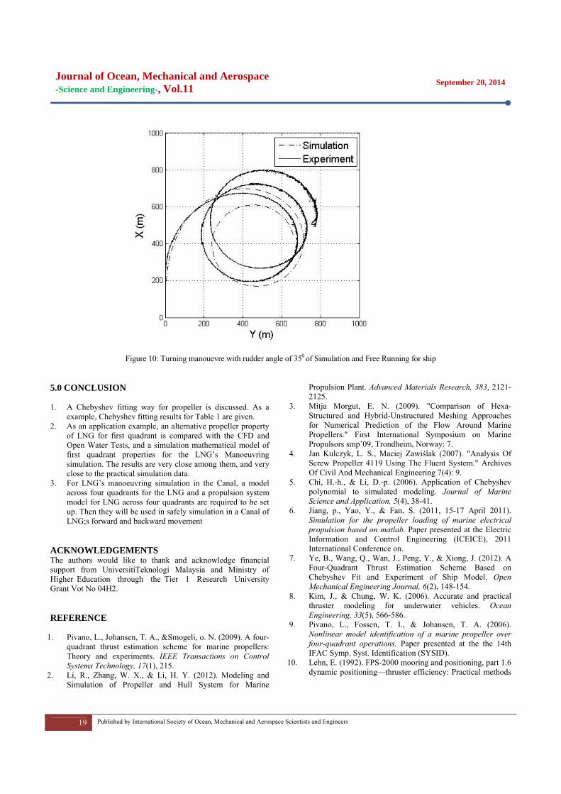
Comparison between simulated and free running results was illustrated in Figures 8 and 9. Zig-zag manouevre for 10° and 20° rudder angle and turning manouevre for a 35° rudder angle are shown in Figures 8 and 9, respectively. Generally speaking, the trends of free running tests in 35° rudder angle turning manoeuvre; and zig-zag manoeuvre for 10° and 20° rudder angle were quite similar to those of the simulation results.

Figure 9: Comparison zig-zag manouevre with 100 and 200 rudder angle between Simulation and Free Running


September 20, 2014


Figure 10: Turning manouevre with rudder angle of 350 of Simulation and Free Running for ship

5.0 CONCLUSION 1. A Chebyshev fitting way for propeller is discussed. As a

example, Chebyshev fitting results for Table 1 are given. 2. As an application example, an alternative propeller property

of LNG for first quadrant is compared with the CFD and Open Water Tests, and a simulation mathematical model of first quadrant properties for the LNG’s Manoeuvring simulation. The results are very close among them, and very close to the practical simulation data.

3. For LNG’s manoeuvring simulation in the Canal, a model across four quadrants for the LNG and a propulsion system model for LNG across four quadrants are required to be set up. Then they will be used in safely simulation in a Canal of LNG;s forward and backward movement

ACKNOWLEDGEMENTS The authors would like to thank and acknowledge financial support from UniversitiTeknologi Malaysia and Ministry of Higher Education through the Tier 1 Research University Grant Vot No 04H2. REFERENCE

1. Pivano, L., Johansen, T. A., &Smogeli, o. N. (2009). A four-quadrant thrust estimation scheme for marine propellers: Theory and experiments. IEEE Transactions on Control Systems Technology, 17(1), 215.

2. Li, R., Zhang, W. X., & Li, H. Y. (2012). Modeling and Simulation of Propeller and Hull System for Marine

Propulsion Plant. Advanced Materials Research, 383, 2121-2125.

3. Mitja Morgut, E. N. (2009). "Comparison of Hexa-Structured and Hybrid-Unstructured Meshing Approaches for Numerical Prediction of the Flow Around Marine Propellers." First International Symposium on Marine Propulsors smp’09, Trondheim, Norway: 7.

4. Jan Kulczyk, L. S., Maciej Zawiślak (2007). "Analysis Of Screw Propeller 4119 Using The Fluent System." Archives Of Civil And Mechanical Engineering 7(4): 9.

5. Chi, H.-h., & Li, D.-p. (2006). Application of Chebyshev polynomial to simulated modeling. Journal of Marine Science and Application, 5(4), 38-41.

6. Jiang, p., Yao, Y., & Fan, S. (2011, 15-17 April 2011). Simulation for the propeller loading of marine electrical propulsion based on matlab. Paper presented at the Electric Information and Control Engineering (ICEICE), 2011 International Conference on.

7. Ye, B., Wang, Q., Wan, J., Peng, Y., & Xiong, J. (2012). A Four-Quadrant Thrust Estimation Scheme Based on Chebyshev Fit and Experiment of Ship Model. Open Mechanical Engineering Journal, 6(2), 148-154.

8. Kim, J., & Chung, W. K. (2006). Accurate and practical thruster modeling for underwater vehicles. Ocean Engineering, 33(5), 566-586.

9. Pivano, L., Fossen, T. I., & Johansen, T. A. (2006). Nonlinear model identification of a marine propeller over four-quadrant operations. Paper presented at the the 14th IFAC Symp. Syst. Identification (SYSID).

10. Lehn, E. (1992). FPS-2000 mooring and positioning, part 1.6 dynamic positioning—thruster efficiency: Practical methods


September 20, 2014


for estimation of thrust losses: Technical Report 513003.00. 06. Marintek, SINTEF, Trondheim, Norway.

11. Seo, J. H., Seol,D.M. ,Lee,J.H., Rhee,S.H. (2010). Flexible CFD meshing strategy for prediction of ship resistance and propulsion performance. Inter J Nav Archit Oc Engng, 2, 139-145.

12. Zadravec, S. B., M. Hribersek (2007). The Influence of Rotating Domain Size of in a Rotating Frame of Reference Approach for Simuation of Rotating Impeller in a Mixing Vessel. Journal of Engineering Science and Technology, 2, 126-138.

13. Paik, B.G., Kim, G.D., Kim, K.S., Kim, K.Y., Suh, S.B. (2012). Measurements of the rudder inflow affecting the rudder cavitation. Ocean Engineering, 48, 1-9.

14. W.P.A. van Lammeren, J.D. van Manen, M.W.C. Oosterveld. (1969). The Wageningen B-screw series, Trans. SNAME, 77, pp. 269–317.

15. Fujino, M., 1968, "Experimental studies on ship manoeuvrability in restricted waters-Part 1", International Shipbuilding Progress, Vol.15, No.168, pp.279-301.

16. Duffy, J.T, 2002. Prediction of bank induced sway force and yaw moment for ship handling simulator. Ship Hydrodynamics Centre, Australian Maritime College (AMC).

17. PIANC, 1992. Capability of ship manoeuvring simulation models for approach channels and fairways in harbours. Report of Working Group no. 20 of Permanent Technical Committee II, Supplement to PIANC Bulletin No. 77, pp. 49

18. Maimun, A, Priyanto, A, et. al (2013). A mathematical model on manoeuvrability of a LNG tanker in vicinity of bank in restricted water, Safety Science 53, 34-44.


September 20, 2014


Motion of Ship-Shaped Floating Liquefied Natural Gas

Jaswar Koto,a,*

a)Ocean and Aerospace Engineering Research Institute, Indonesia b)Mechanical Engineering, Universiti Teknologi Malaysia *Corresponding author: [email protected] Paper History Received: 2-September-2014 Received in revised form: 14- September -2013 Accepted: 17- September -2014 ABSTRACT Floating Liquefied Natural Gas (LNG) recently are new in the offshore platform and operation, since it is new so it is important to analyzed the stability and seakeeping of this vessel. This project are conducting stability assessment and seakeeping of Floating Liquefied Natural Gas (LNG) with initially it has to design the hull by referring the basic dimension of FPSO KIKEH that located at the 120 km northwest of Labuan Island which is the environmental location of this project. Hence this project are using Maxsurf for designing the hull, Hydromax to do stability assessment and Seakeeper for seakeeping analysis which is to generate wave spectrum and Response Amplitude Operator and hence to analyzed the motion characteristic of this vessel behavior in the research location. KEY WORDS: Floating Production Storage Offloading; Seakeeping; Stability. NOMENCLATURE FLNG Floating Liquefied Natural Gas FPSO Floating Production Storage Offloading LPG Liquefied Petroleum Gas LNG Liquefied Natural Gas RAO Response Amplitude Operator IMO International Maritime Organization VLCC Very Large Crude Oil Carrier

1.0 INTRODUCTION Floating Liquefied Natural Gas is the floating natural gas vessel that has same functioning and technology of Floating Production Storage Offloading vessel but the difference between two of them is this FPSO are their processing petroleum and gas also they are producing the Petroleum and transfer these product to the LPG or LNG tankers. Then the FLNG vessel is that has same technology of processing and producing, but they are focusing on the natural gas only. Furthermore FLNG are the floating platform that has facilities processes gas into liquids, this platform also functioning to store this liquids gas in the platform and this platform producing LNG in offshore area.

The important to establish the Floating Liquefied Natural Gas rather that the LNG conventional facilities are to reducing the total cost operating of the operation due to the less using pipelines that been using in the conventional facilities, and FLNG has the special functioning, let say if the field of the source are depleted, this vessel can be moved to the new location that has new source.

Usually this vessel is not moving but then it’s in the condition of static, so in order to get this vessel in stable condition the research has to be investigate the adequate stability of vessel this will include the intact stability and also the hydrodynamic consideration of the vessel. This is because this vessel is located at the sea condition that has irregular sea condition that we not been able to predict. Moreover this vessel facilities has various liquid that tend to be flame or blow if design of the vessel and the choice making of sea condition not properly been choose, if we choose the high beam that has recently bad condition weather this vessel will collapse of capsize due to the high beam of wave.

Stability is one most mandatory design stage that needed to be carefully done by the designer in order to maintain the vessel in the upright position for long time of period because the failure of the stability on the vessel may cause many facilities above deck, under deck, mooring lines and turret for Floating Liquefied Natural Gas.

Based on my study, found that there is two problem that usually faced by the designer regarding the stability of the


September 20, 2014


floating LNG vessel there are environmental impact on the big vessel like VLCC hull type which is effect on the stability and lastly are problem on the hull design, when it operate on the seaworthiness it roll angle excessive of more the 5° of rolling angle.

The objectives of the project were to design hull of Floating LNG by using basic dimension from FPSO KIKEH, based on the stability assessment by IMO criteria and determine wave spectra of Roll, Pitch and Heaving by using Pierson-Moskowitz formula, determine Response Amplitude Operator of heave, pitch and rolling motion and analyze motion characteristics in term of heaving, rolling and pitching in head, beam, and following seas.

The scope of study for this project will focus on the motion and stability of Floating Liquefied Natural Gas vessel motion of heave, pitch and roll motion. Furthermore, for this analysis we located the location of analysis at South Sea of China, the specific location is at 120 kilometers northwest of Labuan. Then, Figure.1 showed the picture of the exact location of the analysis; this picture was taken from Google Earth. Moreover, this project will cover ship condition in lightship and full load condition.

Figure.1: Location of FPSO KIKEH.

2.0 SIMULATION This paper calculated and analyzed using commercial software which is MAXSURF for designing the model of floating LNG, HYDROMAX for stability assessment and SEAKEEPER for estimation Response Amplitude Operation and wave spectrum analysis.

In the simulation, wave data is collected from the Malaysia Metrology Department of Malaysia. All the data are the wave data, which is, contain the wind speed, wave period and wave frequency, which is the data from 1995 until 2008. Then all the data are analyzed by using Microsoft excel to get the significant wave data. Thus, Table.1 is the data that are been analyzed and summarized indicate the environment condition.

Moreover, after the wave, data were collected then the initial designs of Floating LNG are begin by using MAXSURF software. These designs are not fully design but it is design by using basis ship that taken from MAXSURF design that is the VLCC design of hull. So the detailed information about the design particular will be discussed.

Then the next step, are when finish the design of floating LNG,

the generating the offset data from MAXSURF software. This offset data are important to use in the calculation of equation of motion. Then after all, the offset data been set, hydrostatic data need to be generated or calculated by using HYDROMAX software. This hydrostatic data are important to overview the characteristic of vessel when in the static condition.

Then the project will proceed to the stability calculation and assessment by using HYDROMAX and calculation. From the HYDROMAX the stability assessment will carried out the GZ curve analysis by using IMO criteria that usually using for indicating the stability of the vessel. Then after the stability then proceed to calculate the added mass of the vessel by using the SEAKEEPING software that will generate the result of added mass of vessel.

Figure.2: Flowchart to analyze Floating LNG

Table.1: Environmental Condition

Return Period (year)

Wind speed (knot)

Wave period (sec)

Wave height (meter)

1 30 8 3.5 10 45 14 4 100 45 14 4

After analyzing and calculating added mass of vessel, wave spectrum and wave encounter spectrum by using JONSWAP formula were estimated using the SEAKEEPER software. This software analyzed motion of the vessel such as rolling, pitching and heaving. 3.0 RESULT AND DISCUSSION


September 20, 2014


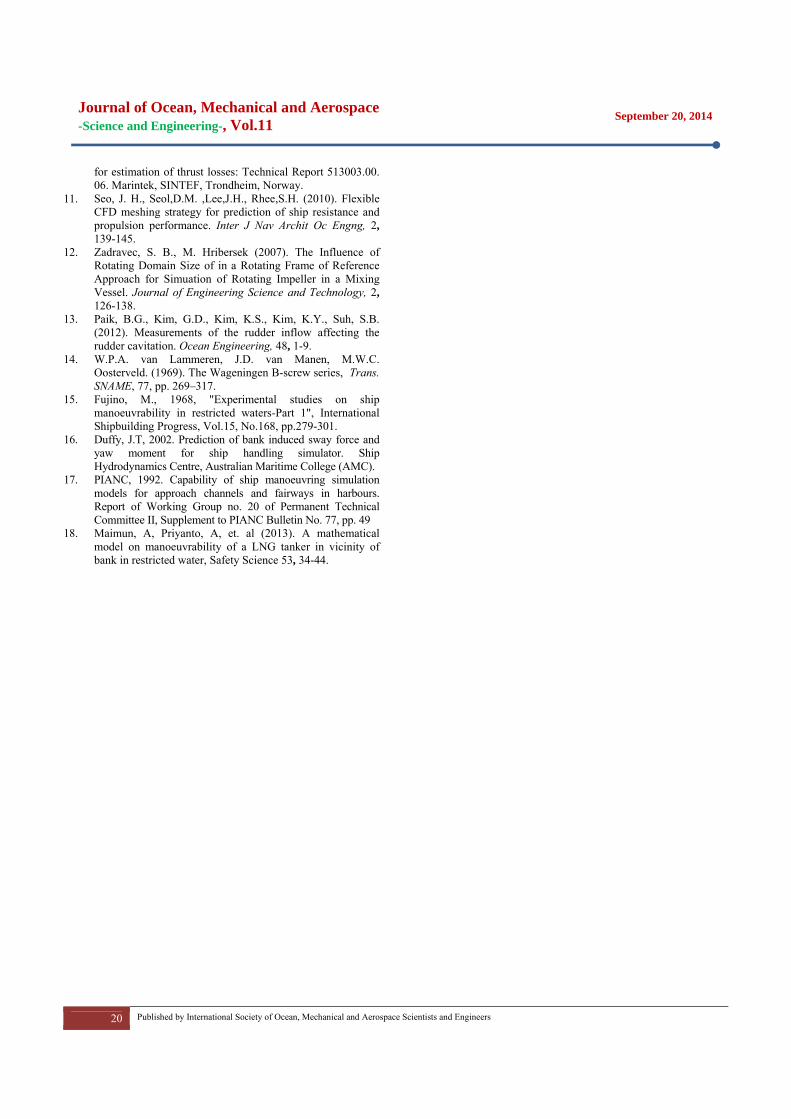
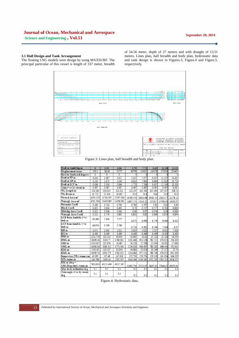
3.1 Hull Design and Tank Arrangement The floating LNG models were design by using MAXSURF. The principal particular of this vessel is length of 337 meter, breadth

of 54.56 meter, depth of 27 meters and with draught of 13.51 meters. Lines plan, half breadth and body plan, hydrostatic data and tank design is shown in Figures.3, Figure.4 and Figure.5, respectively.

Figure.3: Lines plan, half breadth and body plan.

Figure.4: Hydrostatic data.


September 20, 2014


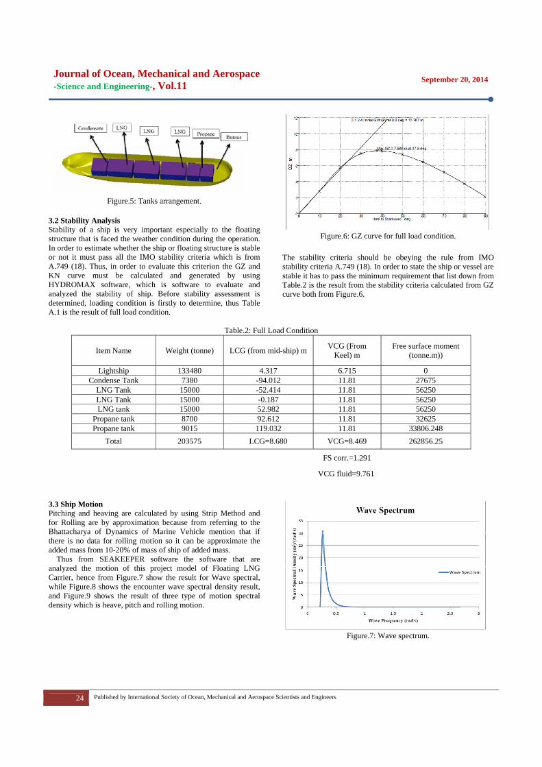
Figure.5: Tanks arrangement.

3.2 Stability Analysis Stability of a ship is very important especially to the floating structure that is faced the weather condition during the operation. In order to estimate whether the ship or floating structure is stable or not it must pass all the IMO stability criteria which is from A.749 (18). Thus, in order to evaluate this criterion the GZ and KN curve must be calculated and generated by using HYDROMAX software, which is software to evaluate and analyzed the stability of ship. Before stability assessment is determined, loading condition is firstly to determine, thus Table A.1 is the result of full load condition.

Figure.6: GZ curve for full load condition.

The stability criteria should be obeying the rule from IMO stability criteria A.749 (18). In order to state the ship or vessel are stable it has to pass the minimum requirement that list down from Table.2 is the result from the stability criteria calculated from GZ curve both from Figure.6.

Table.2: Full Load Condition

Item Name Weight (tonne) LCG (from mid-ship) m VCG (From Keel) m

Free surface moment (tonne.m))

Lightship 133480 4.317 6.715 0 Condense Tank 7380 -94.012 11.81 27675

LNG Tank 15000 -52.414 11.81 56250 LNG Tank 15000 -0.187 11.81 56250 LNG tank 15000 52.982 11.81 56250

Propane tank 8700 92.612 11.81 32625 Propane tank 9015 119.032 11.81 33806.248

Total 203575 LCG=8.680 VCG=8.469 262856.25

FS corr.=1.291

VCG fluid=9.761 3.3 Ship Motion Pitching and heaving are calculated by using Strip Method and for Rolling are by approximation because from referring to the Bhattacharya of Dynamics of Marine Vehicle mention that if there is no data for rolling motion so it can be approximate the added mass from 10-20% of mass of ship of added mass.

Thus from SEAKEEPER software the software that are analyzed the motion of this project model of Floating LNG Carrier, hence from Figure.7 show the result for Wave spectral, while Figure.8 shows the encounter wave spectral density result, and Figure.9 shows the result of three type of motion spectral density which is heave, pitch and rolling motion.

Figure.7: Wave spectrum.


September 20, 2014


Figure.8: Encounter wave spectrum.

In order to know whether this vessel is suitable to operate at the desired location of the research it is essential to generate the Response Amplitude Operator (RAO) of the ship. Hence, RAO of the ship was analyzed by SEAKEEPER Software, which generate three different types of RAO motions, which are heave, pitching and rolling motion. The result for RAO four types of wave heading which are 0°, 60°, 90° and 18°0 wave heading are shown in Figures.9, 10, and 119.

Figure.9: Wave Spectrum for heave, pitch and rolling motions.

Figure.8: RAO result for 0° wave heading.

Figure.10: RAO result for 60° wave heading.

Figure.11: RAO for 90° wave heading

Table.3: Added mass for heave, pitch and rolling motion.


September 20, 2014


Table.4: IMO Stability Criteria IMO Stability Criteria Result

Criteria Required Lightship Status Full Load Status Area 0 to 30 Shall not less than 3.151 [m.deg] 190.468 [m.deg] PASS 123.868[m.deg] PASS Area 0 to 40 shall not be less than 5.157 [m.deg] 313.482 [m.deg] PASS 201.454[m.deg] PASS Area 30 to 40 shall not be less than 1.719 [m.deg] 123.014 [m.deg] PASS 77.586[m.deg] PASS Maximum GZ at 30 or greater shall not be less than 0.2 [m.deg] 11.667 [m.deg] PASS 7.491[m.deg] PASS Angle of maximum GZ Shall not be less than 25 [deg] 41.6 [deg] PASS 37.8[deg] PASS Initial GMtranverse Shall not be less than 0.35 [m] 24.952 [m] PASS 15.767[m] PASS 5.0 CONCLUSION Finally, from this Stability of Floating Liquefied Natural Gas (LNG) projects are concluding that: 1. Hull of Floating LNG was successfully design by using

Maxsurf. 2. Wave spectrums for roll, pitch and heaving motion have

been identified by using Pierson – Moskowitz wave spectra. 3. This Floating LNG is stable and safe to operate production

facilities with pass all the IMO stability criteria. 4. Response Amplitude Operator (RAO) for heave, pitching

and rolling motion was identified and analyzed. 5. Rolling angle of Motion Characteristic analysis was

identified and archived the degree of rolling angle below 3°. . ACKNOWLEDGEMENTS The authors would like to convey a great appreciation to Ocean and Aerospace Engineering Research Institute, Indonesia for supporting this research. REFERENCE 1. Yan, G. and Y. Gu, Effect of parameters on performance of

LNG-FPSO offloading system in offshore associated gas fields. Applied Energy, 2010.87(11): p. 3393-3400.

2. Sheffield, J., Offshore LNG Production – How to Make it Happen. 2005, Gas Processors Association Europe LNG Working Party.

3. Laura Alsobrooks, W.C., Robert Garrity, Steven Krafft, Deborah McElligott, William Ray, Design of a Floating Liquefied Natural Gas Production Vessel for Timor Sea. 2009, Texas A&M University: Texas, U.S.A.

4. Shell to deploy FLNG technology in Australia. Pump Industry Analyst, 2009(10): p. 3-4.

5. Halkyard, J., Floating offshore design, in Handbook of Offshore Engineering, S. Chakrabarti, Editor. 2005, Elsevier Ltd: Houston, TX, USA.

6. Library, N.M., Beaufort, M.D.o. UK, Editor. 2010: UK. 7. Chakrabakti, S., Handbook of Offshore Engineering. Ocean

Environment 2005, IL, USA: Elsvier Ltd. 8. Faltinsen, O.M., Hydrodynamics of High-Speed Marine

Vehicles. 2005, Cambridge, UK: Cambridge University Press.

9. Bhattacharya, R., Dynamics of Marine Vehicles 1978, New York.

Publishe

ed & Printed

ISOReJalPekhtt

d OMAse esty Menara Hlan Sisingamakanbaru-Riautp://www.isom

Hotel angaraja No.89u, Indonesia mase.org/

9

Teknik MFakultasUniversIndoneshttp://ft.

Mesin s Teknik itas Riau, ia .unri.ac.id/

IISSN: 2354-70065

Vol.11, September.2014 ISSN 2354-7065 - isomase.orgisomase.org/JOMAse/Vol.11 Sep 2014/Vol-11.pdf ·...

Documents

Transcript of Vol.11, September.2014 ISSN 2354-7065 - isomase.orgisomase.org/JOMAse/Vol.11 Sep 2014/Vol-11.pdf ·...