Vol. 53(2), June 2016 OF THE PAKISTAN ACADEMY OF SCIENCES ... · OF THE PAKISTAN ACADEMY OF...
75
PROCEEDINGS B. Life and Environmental Sciences OF THE PAKISTAN ACADEMY OF SCIENCES: ISSN Print : 0377 - 2969 ISSN Online : 2306 - 1448 Vol. 53(2), June 2016 PAKISTAN ACADEMY OF SCIENCES ISLAMABAD, PAKISTAN
Transcript of Vol. 53(2), June 2016 OF THE PAKISTAN ACADEMY OF SCIENCES ... · OF THE PAKISTAN ACADEMY OF...

PROCEEDINGSB. Life and Environmental SciencesOF THE PAKISTAN ACADEMY OF SCIENCES:
ISSN Print : 0377 - 2969 ISSN Online : 2306 - 1448
Vol. 53(2), June 2016
PAKISTAN ACADEMY OF SCIENCESISLAMABAD, PAKISTAN

PAKISTAN ACADEMY OF SCIENCESFounded 1953
President: Anwar Nasim. Secretary General: Zabta K. ShinwariTreasurer: M.D. Shami
Proceedings of the Pakistan Academy of Sciences, published since 1964, is quarterly journal of the Academy. It publishes original research papers and reviews in basic and applied sciences. All papers are peer reviewed. Authors are not required to be Fellows or Members of the Academy, or citizens of Pakistan.
Editor-in-Chief: Abdul Rashid, Pakistan Academy of Sciences, 3-Constitution Avenue, Islamabad, Pakistan; [email protected]
Editors:Animal Sciences: Abdul Rauf Shakoori, University of the Punjab, Lahore, Pakistan; [email protected]
Environmental Sciences: Zahir Ahmad Zahir, University of Agriculture, Faisalabad, Pakistan; [email protected]
Health Sciences: Rumina Hasan, Aga Khan University, Karachi, Pakistan; [email protected]
Plant Sciences: Muhammad Ashraf, Pakistan Science Foundation, Islamabad, Pakistan; [email protected]
Editorial Advisory Board: Zulfiqar A. Bhutta, Department of Paediatrics, University of Toronto, Toronto, Canada; [email protected]
Adnan Hayder; Johns Hopkins Center for International Injury Research Unit, Baltimore, Maryland, USA; [email protected]
Rabia Hussain, The Aga Khan University, Karachi, Pakistan; [email protected]
Mateen Izhar; Sheikh Zayed Medical Complex, Lahore, Pakistan; [email protected]
Philippe Monneveux, International Potato Center, Lima, Peru; [email protected]
Munir Ozturk, Department of Botany, Ege University, Izmir, Turkey; [email protected]
Omrana Pasha: Johns Hopkins Bloomberg School of Public Health, Baltimore, USA; [email protected]
Muhammad Qaisar, University of Karachi, Karachi, Pakistan; [email protected]
Mohammad Wasay, The Aga Khan University, Karachi, Pakistan; [email protected]
Youcai Xiong, School of Life Sciences, Lanzhou University, Lanzhou 730000, Gansu, China; [email protected]
Annual Subscription: Pakistan: Institutions, Rupees 2000/- ; Individuals, Rupees 1000/- Other Countries: US$ 100.00 (includes air-lifted overseas delivery)
© Pakistan Academy of Sciences. Reproduction of paper abstracts is permitted provided the source is acknowledged. Permission to reproduce any other material may be obtained in writing from the Editor-in-Chief.
The data and opinions published in the Proceedings are of the author(s) only. The Pakistan Academy of Sciences and the Editors accept no responsibility whatsoever in this regard.
HEC Recognized, Category X; PM&DC Recognized
Published by Pakistan Academy of Sciences, 3 Constitution Avenue, G-5/2, Islamabad, PakistanTel: 92-5 1-9207140 & 9215478; Fax: 92-51-9206770; Website: www.paspk.org
Printed at PanGraphics (Pvt) Ltd., No. 1, I & T Centre, G-7/l, Islamabad, PakistanTel: 92-51-2202272, 2202449 Fax: 92-51-2202450 E-mail: [email protected]
C O N T E N T SVolume 53, No. 2, June 2016 Page
Research Articles
Environmental Sciences
Performance Assessment of Municipal Solid Waste Management Model of Lahore: 69A Case Study of Two Turkish Contractors— Sajjad Haydar, Misbah Afaq, Ghulam Hussain, and Ghayas Ahmad
Inactivation of Escherichia coli and Salmonella with Chlorine in Drinking Waters at 83Various pH and Temperature Levels— Sajida Rasheed, Imran Hashmi, and Luiza Campos
Wastewater Characterization of Selected Industries in Quaid-e-Azam Industrial Estate: 93Treatment Options and Impact on Groundwater Quality— Sajjad Haydar, Ghulam Hussain, Husnain Haider, and Attiq-ur-Rehman
Health Sciences
Microbiological Evaluation of Raw Meat Products Available in Local Markets of 103Karachi, Pakistan— Ayesha Zafar, Erum Ahmed, Hafiza Wajiha, Abdul Basit Khan
Plant Sciences
New Fungal Records on Psidium guajava from Pakistan 111— Syed Qaiser Abbas, Abida Perveen, Sana Riaz, Thereema Iftakhar, and Alia Abbas
Wakeby Distribution Modelling of Rainfall and Thunderstorm over Northern Areas of Pakistan 121— Naeem Sadiq
Climatic Variability and Linear Trend Models for the Six Major Regions of Gilgit-Baltistan, Pakistan 129— Muhammad Raza, Dostdar Hussain, and Ghulam Rasul
Instructions for Authors 137
Submission of Manuscripts: Manuscripts may be submitted online as E-mail attachment. Authors must consult the Instructions for Authors at the end of this issue or at the Website: www.paspk.org
PROCEEDINGSOF THE PAKISTAN ACADEMY OF SCIENCES:B. Life and Environmental Sciences


Research Article
Proceedings of the Pakistan Academy of Sciences: Pakistan Academy of SciencesB. Life and Environmental Sciences 53 (2): 69–81 (2016)Copyright © Pakistan Academy of SciencesISSN: 0377 - 2969 (print), 2306 - 1448 (online)
————————————————Received, July 2015; Accepted, June 2016*Corresponding author: Sajjad Haydar; Email: [email protected]
Performance Assessment of Municipal Solid Waste Management Model of Lahore: A Case Study of Two Turkish Contractors
Sajjad Haydar*, Misbah Afaq, Ghulam Hussain, and Ghayas Ahmad
Institute of Environmental Engineering & Research, University of Engineering & Technology, Lahore, Pakistan
Abstract: The solid waste management (SWM) trends are changing rapidly in big urban centers. For improving efficiency of service delivery,invariably the collection and transportation services are outsourced to private contractors. The Lahore Waste Management Company (LWMC) also outsourced their services to two Turkish contractors: Contractor-A and Contractor-B. The objective of this study was to evaluate the performance of these contractors. For this purpose two (02) performance assessment models were developed; one for service recipients and second for SWM contractor’s staff. Key performance indicators (KPIs), as developed by the LWMC, were evaluated and the relevant indicators concerning techno-social aspects were selected corresponding to each model, to assess the service delivery level by the contractors. A questionnaire was developed for each model. Data was collected from 40 Union Councils (UCs) of Lahore. 384 service beneficiaries and 68 concerned officials were interviewed from all the selected UCs. The Statistical Package for Social Sciences (SPSS) was used for data analysis. The analysis revealed that from the service beneficiary point of view, the service delivery is satisfactory, however requires certain improvements. It is also deduced that overall performance of both the SWM contractors is encouraging; however, they need improvements primarily in some sectors, like public awareness plans, staff trainings and availability of vehicles and equipment. Overall, performance of Contractor-B is better in all KPIs as compared to the Contractor-A.
Keywords: solid waste management (SWM), Turkish SWM contractors, performance assessment, consumer satisfaction, LWMC, service delivery in SWM
1. INTRODUCTION
More than half of the world’s population lives in urban areas. Urban population growth rate varies among countries and regions. In south Asian countries, over the past 50 years, urban population has grown by about 300 million people. As the region’s population has become more urbanized, the number and size of the cities has increased as well as generation rate of municipal solid waste (MSW) [1]. Management of solid waste has emerged as a major environmental issue in big urban settings.
Lahore is the second largest city of Pakistan. Its population is around 9 million [2]. The daily municipal solid waste generation in Lahore city is about 5500 tons [3].The responsibility of solid waste management in Lahore remained with the City District Government till 2010. A study in year 2007 revealed that only 70% of the waste, generated in Lahore, was collected and sent to
open dumping sites (Mehmood Booti Dumpsite, Baggrian Dumpsite, Saggian Dumpsite and Tibba Dumpsite); the rest remained on streets, roads or open spaces. The open dumping sites turned into breeding grounds for disease vectors, communication of different diseases and produced objectionable odours. Furthermore, household waste was mostly collected through hand carts or donkey carts and municipality did not have modern and sufficient waste collection equipment [4].
Main reasons of poor MSW management in Lahore includes: (1) lack of strong commitment on the part of government to introduce institutional and management reforms for managing urban waste; and (2) lack of modern storage,collection and transportation equipment.
Realizing the aforementioned situation, City District Government Lahore (CDGL) established a corporate body ‘Lahore Waste Management
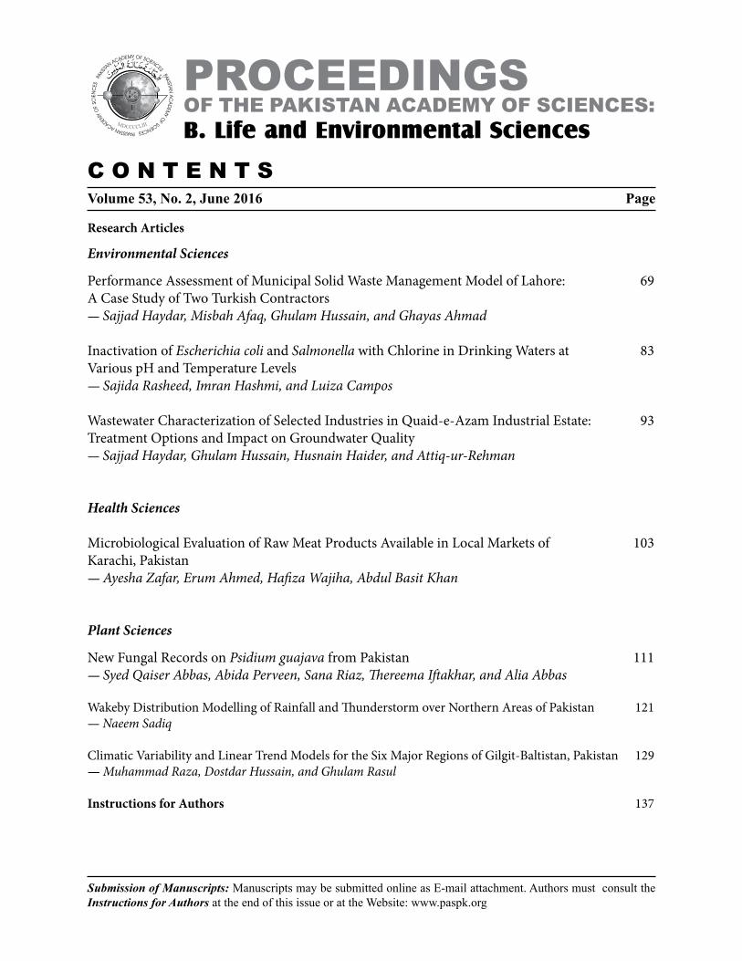
Company (LWMC)’ on 19th March 2010 for waste management service delivery in Lahore. It was a new institutional set up with professionals hired on market based remunerations. Modern management tools like vehicle tracking & management system, android phones, complaint registration and redress systems were employed. For the purpose of operations, the entire Lahore was divided into two zones (Fig. 1). Ferozpur Road is the dividing line for the two (02) zones. Two (02) Turkish companies Contractor-A and Contractor-B,were hired and were entrusted with zone-1 and 2, respectively.
These contractors appear to play an efficient role to improve the SWM in the city, however there are still some concerns regarding reforms brought about by these contractors at various levels [5]. They are paid USD 25 per ton of the waste collected. This cost is often criticized to be on higher side. The cost figure reported from within Pakistan lies in a range of USD 10 to 15 per ton. However, the service delivery standards for lower cost is also inferior From the neighboring country India, the cost in Mumbai is USD 44 per ton by Municipal Corporation Greater Mumbai [6]; in Chennai it
is USD 33 per ton by Corporation of Chennai[7]and another figure reported from India is USD 16 per ton[8]. It is also noted that inclusion of private sector and community may reduce the cost per ton by about 30% [6-8].
After the establishment of LWMC and outsourcing of collection and transportation to the Turkish contractors, there was no systematic study conducted to evaluate the performance of the new arrangement for solid waste management in Lahore. Thus, the present study aimed at evaluating the performance and identifying areas for further improvement.
2. MATERIALS AND METHODS
To achieve the objectives of study two (02) performance assessment models were developed i.e. service recipients assessment model; and service contractor’s competence assessment model [9].These models consider both social and technical inputs. The first model addresses expectations and judgment of the service beneficiary. Second model is devoted to attributes and performance of the
Fig. 1. Zoning of Lahore for SWM. (Source: Planning Section, SWM Department, CDGL)
Zone-2 Zone-1
70 Sajjad Haydar et al

contractors. Both of these models rely on the views of service beneficiaries and concerned officials and do not rely on self-observation.
2.1 ServiceBeneficiaryAssessmentModel (SBAM)
This model considers views and degree of satisfaction with the SWM service as expressed by the service beneficiaries and builds upon the key performance indicators (KPIs) pointed out in Table 1. On the basis of KPIs stated in Table 1, a questionnaire was developed for SBAM. This questionnaire was designed on three (03) point Likert Scale [13-16]. Each question contained different expected answers based on the degree of satisfaction of service beneficiaries.
After the development of questionnaire, the study area was selected for survey and to fill the questionnaires. It was selected on the basis of Purposive Sampling. Purposive sampling is a sampling method in which elements are chosen from among the whole population based on purpose of the study. The main objective of purposive sampling is that the researcher, with his good decision and appropriate policy, chooses those elements which are meant for fulfilling the research objective [17]. Lahore has nine (09) towns containing 146 Union Councils (UCs) [18]. Total forty (40) UCs were selected from all the nine (09) towns. Twenty (20) UCs were selected for each contractor i.e. 20 for Contractor-A and 20 for Contractor-B. The selected UCs for both contractors are listed in Table 2.
After selection of the study area, the sample size (i.e., number of people to be interviewed) was calculated. The present population of the selected UCs was calculated by using the population data of 1998 Census Report [19]. The Sample Size of 384 people was computed, using 95% confidence level [20].
2.2 Service Contractor’s Competence Assessment Model (SCCAM)
This Model assesses the contractor’s ability based on six (06) KPIs, considered to be the main factors that influence the contractor’s performance. These KPIs are enlisted in Table 3. On the basis of aforementioned KPIs, a sample questionnaire for Service Contractor’s Competence Assessment Model (SCCAM) was developed using three (03) point Likert Scale. The sample
size for 90% confidence level came out to be 68. A lower confidence level (90%) for SCCAM, when compared with SBAM (95%), was used. The reason was availability of backup data for all answers obtained from concerned officials of both SWM contractors, hence justified. These questionnaires were filled for concerned officials of selected UCs, i.e.,by officials from the offices of Contractor-A, Contractor-B and LWMC.
2.3 Data Entry and Analysis
After the questionnaire surveys and interviews, all the data were entered in the Statistical Package for the Social Sciences (SPSS) software for analysis [21].
3. RESULTS AND DISCUSSION
3.1 ServiceBeneficiaryAssessmentModel (SBAM)
The results,based on SPSS analysis, are presented in this section. As stated already, 384 service beneficiaries were interviewed from forty (40) UCs. Out of these, 345 were males and 39 females; out of these 384 total beneficiaries, 317 were literate and 67 illiterate. The details of the findings based on SPSS analysis are discussed in the following sections:
3.1.1 Public Awareness on SWM Operations
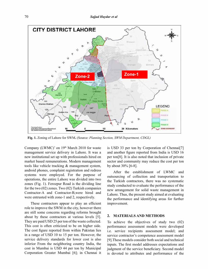
i. Details of public awareness are presented in Fig. 2. It can be seen that about 49% respondents from the Contractor-A and 53% from the Contractor-B service area, were aware about the working of private contractors. No response was received from some segment of the respondents. Thus the performance can be ranked as “average” on this KPI (Table 4). It warrants greater efforts on the part of LWMC and the contractors on awareness issue.
ii. In the Contractor-B service area, the public of Garden Town UC was found most aware and Shahdara UC least aware. Whereas community of Race Course UC was found most aware and Al-Faisal Town UC least aware in the Contractor-A service area. Public awareness campaigns were not launched in the area; it was reported by many respondents.
iii. Fig. 3 shows the state of general cleanliness
Assessment of Solid Waste Management Model in Lahore 71

Table 3. KPIs for SCCAM.Sr. No. KPI Description1 Public awareness plans Formulation of public awareness plans on regular
basis2 Work operation strategies and practices Quality of work operations and practices;
operations monitoring, optimized operational plans and continuous evaluation.
3 Training of employees Existence of training programs for capacity development of the employees
4 Protection of public health and the environment
Ensuring use of personal protective equipment in operation by the concerned officials.
5 Equipment and facilities owned by the contractor
Quality of equipment and facilities % of the actual machinery deployed in comparison with the machinery to be deployed as per contract
6 Solid waste collected and disposed % of waste collected and disposed.
Table 1. KPIs for SBAM.Sr. No. KPI Description
1 Public awareness on SWM operations % of the people aware of the Contractor’s operation
2 General cleanliness of the service area % of people satisfied with the level of cleanliness in the area
3 Acceptability of the quality of the service % of people satisfied with the quality of service of the contractors in their area
4 Quality of customer service % of people satisfied with the customer service
Table 2. Union councils selected for the study.
Sr. No. Zone-1 (Contractor-A) Zone-2 (Contractor-B)Town Union council Town Union council
1 Data Ganj Baksh Race CourseData Gunj Baksh
Riwaz Garden2 Mozang Bilal Gunj3 Gulberg Gulberg Sanda Khurd4 Naseer Abad
GulbergFaisal Town
5
Shalimar
Crown Park Pindi Rajputan6 Mujahidabad Garden Town7 Begum Pura
Samanabad
Gulshan-e-Iqbal8 Baghbanpura Muslim Town9
Aziz Bhatti
Taj Bagh Nawan Kot10 Al-Faisal Town New Samanabad11 Harbanspura
Allama IqbalTownship
12 Mughalpura Johar Town13 Ravi Siddique Pura Niaz Beg14 Rang Mahal Sabzazar15
Wagah
Muslim AbadRavi
Aziz Colony16 Darogha Wala Shahdara17 Salamat Pura Kot Begum18 Lakho Dhair
NistharGreen Town
19 Nishtar Sittara Colony Chandrai20 Dulu Kalan Khurd Farid Colony
72 Sajjad Haydar et al
Contractor-A Contractor-B
Fig. 2. Public awareness on SWM operations.
Contractor-A Contractor-B
Fig. 3. Respondent’s views regarding the extent of cleanliness.
Low Income UCs Average Income UCs High Income UCs
Fig. 4. Public satisfaction on income level basis in OZAPK service area.
Assessment of Solid Waste Management Model in Lahore 73

in the service areas of each contractor. It is clear that respondents from the area where Contractor-B is operating were found more satisfied regarding the cleanliness of their area as compared to Contractor-A;since 45% respondents from Contractor-B and 41% from Contractor-A service area said that their areas remain clean. The performance for this KPI, for both the contractors, fall in the “average” category. It shows more efforts are required on the part of both contractors. The answer, moderately clean, was not included in performance evaluation.
iv. Public satisfaction with the extent of cleanliness was higher in affluent neighborhoods as compared with low and average income areas. In the Contractor-B service area, about 28% respondents from low income UCs, 47% from average income UCs and 75% from high income UCs said that their areas remain clean. Whereas in the Contractor-A service area, about 24% respondents from low income UCs, 42% from average income UCs and 77% from high income UCs said that their areas remain clean. Fig. 3 and Fig. 4 show the respondents’ satisfaction on the basis of income level in the service areas of both SWM contractors.
v. Another underlying reason of the good and poor performance of the same contractor in different income group areas was the state of infrastructure facilities (roads, streets, etc.). The extent of cleanliness was found better in the areas with better and wider roads (i.e., Gulberg, Race Course, Garden Town, etc.) as compared to the areas with poor and narrow roads (i.e., Lakho Dhair, Thokar Niaz Beig, etc.).Perhaps, use of small size collection vehicles in low or middle income group could improve the public satisfaction levels in these areas.
vi. However, most of the respondent from the service area of both SWM contractors said that situation of cleanliness improved in their area
after introducing the private SWM contractors. In addition, current SWM system is modernized to a large extent than the previous system.
3.1.2 Acceptability of Quality of the Service
i. Fig. 6 shows the public satisfaction level. About 45% respondents from the Contractor-B and 38% from Contractor-A service area said that SWM services are of good quality. They revealed that solid waste, at some places,was still collected from the house by the private crew member on donkey carts. Based on the selected Likert scale, the performance of both contractors, for this KPI falls in “average” category.
ii. 49% respondents from Contractor-A and 41% of respondents from Contractor-B service area stated that SWM crew members demand money or any other perks for collection of solid waste from their area.
iii. Almost all respondents suggested that, SWM contractor should provide solid waste collection bags; a practice adopted when these contractors initiated their services in Lahore.
iv. 62% respondents from the Contractor-A area, and 42% from Contractor-B area stated that the capacities and number of storage bin are insufficient. They also stated that locations of the storage bins is inappropriate, i.e., is quite far from their houses. The odour nuisance from these bins was also reported at some places.
v. 84% respondents from the Contractor-A are and 90% from the Contractor-B service area believed that women mobility/privacy is not affected due to the activities of SWM crew in their area. 58% of respondents from the Contractor-A area and 79% from Contractor-B area reported that the SWM crew mostly wear proper uniforms during working hours and their behavior is friendly with them.
74 Sajjad Haydar et al
Table 4. Likert scale used for evaluation.
Sr. No. Likert scale Percentage (%) of peoplesatisfiedwiththeservice
1. Poor performance 0-35
2. Average performance 35-70
3. Good performance 70-100

Low Income UCs Average Income UCs High Income UCs
Fig. 5. Public satisfaction on income level basis in Contractor-A service area.
Contractor-A Contractor-B
Fig. 6. Respondent views regarding the quality of SWM services.
Contractor-A Contractor-B
Fig. 7. Respondent views regarding the overall quality of customer care services.
Assessment of Solid Waste Management Model in Lahore 75

3.1.3 Quality of Customer Service
i. People’s satisfaction with the quality of customer care services is presented in Fig. 7. It can be seen that 44% respondents from the Contractor-B area and 38% from Contractor-A area termed the quality of customer care center as“good”, while the rest either termed it as “average” or “poor”.Thus, the performance for this KPI for both the contractor was found to be “average”.
ii. A significant number of the respondents from the service areas of both the SWM contractors were found unaware regarding existence of any customer care services where complaints could be lodged.
3.2 Service Contractor’s Competence Assessment Model
The findings based on interviews of the concerned officials are discussed in the following sections.
3.2.1 Public Awareness Plans
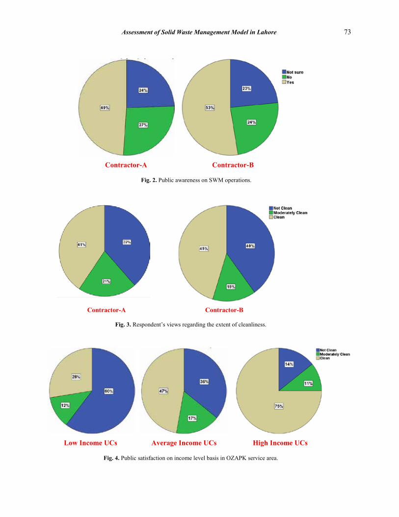
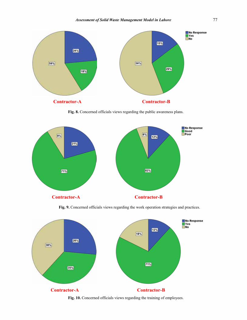
i. Interviews revealed that no proper public awareness plan was formulated by both the SWM contractors. Only 29% concerned officials for Contractor-B and 18% for Contractor-A said that public awareness plan was formulated but no backup data were provided by any concerned official for the verification. Details of concerned official’s views are presented in Fig. 8.
3.2.2 Operation Strategies and Practices
i. The data analysis on this KPI is presented in Fig. 9. It is evident that about 82% concerned officials for Contractor-B and 71% for Contractor-A reported that good work operation strategies and practices have been adopted for SWM in the areas.
ii. The concerned officials, for both the SWM contractors, told that proper route planning was made for the solid waste collection by the vehicle from the allotted area.
iii. The route maps are provided to the drivers for the collection of solid waste in the area and daily log-books are also provided to the drivers for recording trajectory details.
iv. There was a good system for the monitoring
and supervision of the SWM services. As per the information provided by concerned officials field visits are made by the Assistant Mangers (AMs) and Zonal Officer (ZOs) of both SWM contractors in their allotted area, on daily basis.
v. Both the SWM contractors are using the modern tools like GIS, GPS etc. for monitoring and central control. The android mobile phones equipped with GPS facility are provided to the all concerned AMs to track the collection vehicles.
vi. The record of coordination of both SWM contractors were found with other concerned departments like WASA, LWMC, TEPA, etc. but it was limited to the office hours not on 24/7 basis.
3.2.3 Training of Employees
i. The results of this KPI are shown in Fig. 10. About 71% concerned officials for Contractor-B and 35% for Contractor-A told that there is a practice of routine training of employees. However, no backup data was provided by both SWM contractors for the purpose of verification.
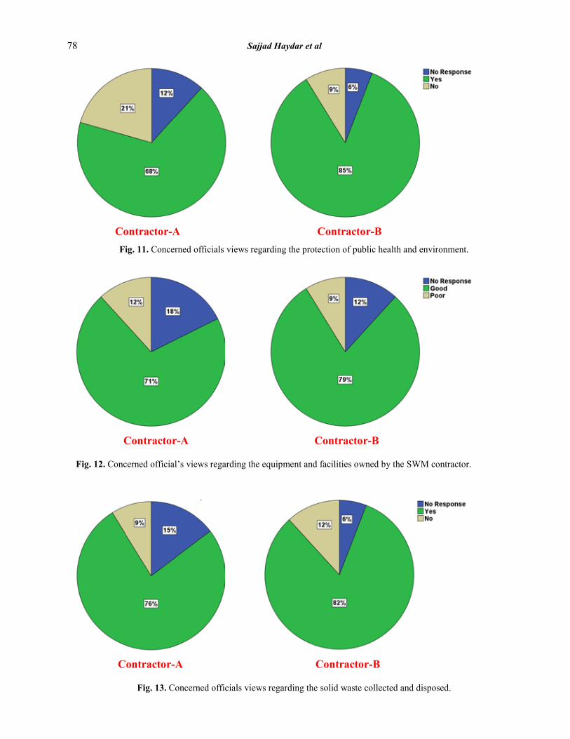
3.2.4 Protection of Public Health and the Environment
i. The results of this KPI are shown in Fig. 11. About 85% officials of Contractor-B and 68% of Contractor-A told that Personal Protective Equipment’s (PPEs), i.e., Gloves, hats, special shoes, masks, special uniform etc. were provided to the all crew members for SWM activities. However, most of the officials also highlighted that, SWM crew members do not use PPEs during routine SWM activities.
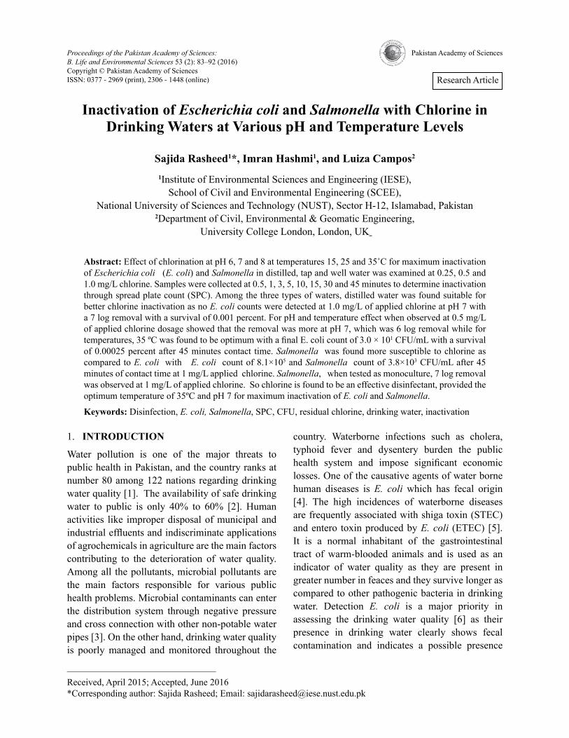
3.2.5 Equipment and Facilities owned by the SWM Contractors
i. Results of this KPI are shown in Fig. 12. About 79% officials of Contractor-B and 71% of Contractor-A told that SWM contractors owned good equipment and facilities for SWM activities.
ii. The officials of both SWM contractors told that vehicle and equipment, being used for the SWM activities are modern, reliable and consistent with the local condition.
iii. The in-house maintenance workshop, for
76 Sajjad Haydar et al
Contractor-A Contractor-B
Fig. 8. Concerned officials views regarding the public awareness plans.
Contractor-A Contractor-B
Fig. 9. Concerned officials views regarding the work operation strategies and practices.
Contractor-A Contractor-B
Fig. 10. Concerned officials views regarding the training of employees.
Assessment of Solid Waste Management Model in Lahore 77
Contractor-A Contractor-B
Fig. 11. Concerned officials views regarding the protection of public health and environment.
Contractor-A Contractor-B
Fig. 12. Concerned official’s views regarding the equipment and facilities owned by the SWM contractor.
Contractor-A Contractor-B
Fig. 13. Concerned officials views regarding the solid waste collected and disposed.
78 Sajjad Haydar et al

vehicles maintenance, was available with both SWM contractors. Contractor-A has two (02) vehicle maintenance workshops on Ferozpur Road. Contractor-B has three (03) workshops; one (01) on Multan Road near Chowk Yateem Khana, one (01) at Outfall Road and one (01) at Valencia Town. However, there was no maintenance schedule for the vehicles. Repairs were carried out only on the observation of any fault.
iv. Officials of both the contractors reported that capacities and number of the solid waste storage containers and vehicles were almost sufficient. However, when the number of vehicles was compared with that given in the contract agreement of both contractors (Table 5), the above statement appeared to be wrong.
3.2.6 Solid Waste Collected and Disposed
i. The results of this KPI are shown in Fig. 13. About 82% concerned officials of Contractor-B and 76% of Contractor-A told that solid waste is properly collected and disposed off.
There are five (05) main solid waste disposal sites in Lahore, i.e., (1) Mehmood Booti Dumping Site; (2) Baggrian Dumping Site; (3) Saggian Dumping Site; (4) Tibba Dumping Site; and (5) Lakho Dhair Landfill Site. Currently, both the contractors have no arrangements for waste recycling. All solid waste is dumped at the dump site without recycling, except at Lakho Dhair.
4. CONCLUSIONS AND RECOMMENDATIONS
Following main conclusions have been drawn on the basis of service beneficiary assessment model:
(1) Almost 50 % of the service beneficiaries on average were unaware regarding the working of SWM contractor and procedure of filing complaints;
(2) Public satisfaction regarding the cleanliness
was more in the high income areas as compare to low income areas;
(3) Extent of cleanliness was better in the areas with better and wider roads;
(4) In some areas private crew members are collecting waste through informal means like donkey carts;
(5) Demand of money or other perks by SWM crew was also highlighted in certain areas;
(6) Odour and nuisance from storage bins was reported at several places;
(7) SWM crew mostly wear proper uniforms during working hours and their behaviour is friendly with public;
(8) Women mobility/privacy is not affected due to the activities of SWM crew; and
(9) Complaints regarding the quality of customer care services were raised by few respondents.
Main conclusions drawn on the basis of service contractor’s competence assessment model include:
(1) No proper public awareness plan was formulated by both SWM contractors and even if they are prepared the public is not duly informed in this regard;
(2) Proper rational route planning was done by both SWM contractors for solid waste collection;
(3) Route maps for solid waste collection and daily log-books for recoding vehicle details were provided to the drivers;
(4) Both SWM contractors were using modern tools for monitoring and centralcontrol;
(5) No comprehensive training plan was formulated by both the SWM contractors;
(6) PPEs were provided and used by the crew members;
(7) Vehicles and equipment being used were modern, reliable and consistent with the local condition but number of vehicles being used was found less as compared to contract
Table 5. Number of vehicles: actually deployed and those written in the contract agreement.
Contractor-B Contractor-B
As per contract Actually deployed As per contract Actually deployed
275 53 234 42
Assessment of Solid Waste Management Model in Lahore 79

documents;
(8) In-house maintenance workshop facility for vehicles maintenance was available for both SWM contractors; and
(9) Recycling of waste is not being carried out by both the contractors. This task should be added in the terms of reference (ToRs) and should be carefully monitored by the LWMC.
The results of this study revealed that both the SWM contractors require improvements in all sectors. However, overall performance of Contractor-B is better in almost all sectors as compared to the Contractor-A.
Following recommendations are made to improve the situation: (1) Effective public awareness campaigns should be launched on large scale and necessary public disclosure of information should be done at all levels; (2) Distribution of solid waste collection bags should be re-started to ensure the better collection of solid waste; (3) Concerned officials should give more attention towards low and average income areas to ensure the cleanliness in addition with arranging suitable machinery that matches with the road width and increase the number of trips of solid waste collection vehicles; (4) The concerned officials should increase their field visit to minimize the complaints regarding the uncleanliness and money demand by the SWM crew members; (5) Capacities and number of storage bins should be increased as per actual demand and should be placed at appropriate locations; (6) Preventive measures should be ensured to stop the odour and nuisance from the storage bins; (7) Both SWM contractors should introduce the reforms to improve quality of their customer care services e.g. online customer service facility. Currently, LWMC is running a website that only provides generic information with less importance given to customer service delivery information and guidance. This online facility can be redesigned to improve the connectivity between the customer and the contractors; (8) The complaint redress data base should be used in optimization of resources and decision making; (9) Comprehensive training plan should be formulated for workers and officials;(10) Number of vehicle and equipment should be increased as per contract documents for material recovery in existing transfer stations can help in start-up of the recycling process; and (11) LWMC may think in terms of formalizing the role
of scavengers and integrate them in their system and use them as its workforce in recycling activities; many such examples exist in other countries [22-30.
5. ACKNOWLEDGEMENTS
The research work was supervised by the first author and is part of a post-graduate research work conducted in IEER, by the last author. The authors are thankful to Managing Director of LWMC, Mr. Khalid Majeed, for his generous help and support without which it was not possible to successfully accomplish this research.
6. REFERENCES1. Muneera, M.N.F. Public-Private Partnership (PPP)
in Solid Waste Management: Literature Review of Experiences from Developing Countries with Special Attention to Sri Lanka. Accessible at: www.diva-portal.org/smash/get/diva2:617746/fulltext01.pdf (2012).
2. LDA. Terms of Reference for Preparation of Integrated Strategic Development Plan for Lahore Region 2035. Accessible at: www.urbanunit.gov.pk/ISDP/TORs%20LAHORE%20LDA_ISDP35_July12-2012pdf (2012).
3. Asim, M., S.A. Batool, & M.N. Chaudhry. Scavengers and their role in the recycling of waste in southwestern Lahore. Resources, Conservation and Recycling 58: 152-162 (2012).
4. Joeng, H. & K. Kim. KOICA-World Bank Joint Study on Solid Waste Management in Punjab, Pakistan. Waste Management, Pakistan, www.urbanunit.gov.pk/PublicationDocs/22.pdf (2007).
5. Nadeem. City Government leaves Lahore in a mess. In: Weekly Pulse, Islamabad (2013).
6. Rathi, S. Alternative approaches for better municipal solid waste management in Mumbai, India. Waste Management 26(10): 1192-200 (2006).
7. S. Esakku, A.S., O. Parthiba & K. Palanivelu. Municipal solid waste managment in Chennai city, India. In: Proceedings Sardinia, 11th International Waste Management and Landfill Symposium, CISA, Environmental Sanitary Engineering Centre, Cagliari, Italy (2007).
8. Furniturwala, I. Setting the trend in waste management; a story from India. In: Waste: The Challenges Facing Developing Countries. http://www.proparco.fr/jahia/webdav/site/proparco/shared/PORTAILS/Secteur_prive_developpement/PDF/SPD15/SPD15_Irfan_furniturwala_uk.pdf
9. Mbuligwe, S.E. Assessment of performance of solid
80 Sajjad Haydar et al

waste management contractors: a simple techno-social model and its application. Waste Management 24(7): 739-749 (2012).
10. Vigderhous, G. The Level of Measurement and ‘Permissible’ Statistical Analysis in Social Research. Pacific Sociological Review 20(1): 61-72 (1996).
11. Vigderhous, G. The level of measurement and ‘permissible’ statistical analysis in social research. Pacific Sociological Review 20(1): 61-72 (1997).
12. Jakobsson, U. Statistical presentation and analysis of ordinal data in nursing research. Scandinavian Journal of Caring Sciences 18: 437-440(2004).
13. Likert, R. A technique for the measurement of attitudes. Archives of Psychology 40: 55 (1932).
14. Nunnally, J.C. Psychometric Theory. McGraw Hill, USA (1978).
15. Clason, D.L., & T.J. Dormody. Analyzing data measured by individual Likert-type items. Journal of Agricultural Education 35(4). http://pubs.aged.tamu.edu/jae/pdf/vol35/35-04-31.pdf (1994)
16. Jacoby, J. and Michael S. Matell, Three-point Likert scales are good enough. Journal of Marketing Research 8(4): 495-500 (1971).
17. Jamieson, S., Likert scales: How to (ab)use them. Medical Education 38(12): 1217-1218 (2004).
18. Singh, N., S. Sood, & V. Kapse. Sampling Techniques: Systematic and Purposive Sampling (a presentation) (2014) Accessible at: http://www.slideshare.net/siddhisood/sampling-techniques-systematic-purposive-sampling-42896131
19. Engineerings, A.C. Union Councils Profile: Lahore, 144 pp. (2013).
20. Population Census Organization, G.O.P. 1998 Census Report, Pakistan (1998).
21. Systems, C.R. Sample Size Calculator. Accessible at: http://www.surveysystem.com/sscalc.htm (1998).
22. IBM. SPSS Software. Accessible at: http://www-01.ibm.com/software/analytics/spss/ (1998).
23. Adan, B., V. Cruz and M. Palaypay. Scavenging in Metro Manila. Manila, Philippines. Report Prepared for Task 11 (1982).
24. Semb, T. Solid Waste Management Plan for the Suez Canal Region, Egypt, In: Recycling in Developing Countries, Thome-Kozmiensk, K. (Ed.). Freitag, Berlin, p. 77-81(1982).
25. Blincow, M. Scavengers and recycling: A neglected domain of production. Labour, Capital and Society 19: 94-115 (1986).
26. Meyer, G. Waste Recycling as a Livelihood in the Informal Sector- The Example of Refuse Collectors in Cairo. Applied Geography and Development 30: 78-94 (1987).
27. Baldismo, J. Scavenging of municipal solid Waste in Bangkok, Jakarta and Manila. Sanitation Reviews, Asian Insitute of Technology, Bangkok: 26 (1988).
28. Mediana, M. Informal recycling and collection of solid waste in developing countries: issues and opportunities, In: Environmental Sanitation Reviews, Asian Institute of Technology, Bangkok; United Nations, Institute of Advanced Studies (1997).
29. Medina, M. Scavenger cooperatives in developing countries. BioCycle: 70-72 (1998).
30. Median, M. Scavenger cooperatives in Asia and Latin America. Resources, Conservation and Recycling 31: 51-69 (2000).
Assessment of Solid Waste Management Model in Lahore 81

Research Article
Proceedings of the Pakistan Academy of Sciences: Pakistan Academy of SciencesB. Life and Environmental Sciences 53 (2): 83–92 (2016)Copyright © Pakistan Academy of SciencesISSN: 0377 - 2969 (print), 2306 - 1448 (online)
————————————————Received, April 2015; Accepted, June 2016*Corresponding author: Sajida Rasheed; Email: [email protected]
1. INTRODUCTION
Water pollution is one of the major threats to public health in Pakistan, and the country ranks at number 80 among 122 nations regarding drinking water quality [1]. The availability of safe drinking water to public is only 40% to 60% [2]. Human activities like improper disposal of municipal and industrial effluents and indiscriminate applications of agrochemicals in agriculture are the main factors contributing to the deterioration of water quality. Among all the pollutants, microbial pollutants are the main factors responsible for various public health problems. Microbial contaminants can enter the distribution system through negative pressure and cross connection with other non-potable water pipes [3]. On the other hand, drinking water quality is poorly managed and monitored throughout the
Inactivation of Escherichia coli and Salmonella with Chlorine inDrinking Waters at Various pH and Temperature Levels
Sajida Rasheed1*, Imran Hashmi1, and Luiza Campos2
1Institute of Environmental Sciences and Engineering (IESE),School of Civil and Environmental Engineering (SCEE),
National University of Sciences and Technology (NUST), Sector H-12, Islamabad, Pakistan2Department of Civil, Environmental & Geomatic Engineering,
University College London, London, UK
Abstract: Effect of chlorination at pH 6, 7 and 8 at temperatures 15, 25 and 35˚C for maximum inactivation of Escherichia coli (E. coli) and Salmonella in distilled, tap and well water was examined at 0.25, 0.5 and 1.0 mg/L chlorine. Samples were collected at 0.5, 1, 3, 5, 10, 15, 30 and 45 minutes to determine inactivation through spread plate count (SPC). Among the three types of waters, distilled water was found suitable for better chlorine inactivation as no E. coli counts were detected at 1.0 mg/L of applied chlorine at pH 7 with a 7 log removal with a survival of 0.001 percent. For pH and temperature effect when observed at 0.5 mg/L of applied chlorine dosage showed that the removal was more at pH 7, which was 6 log removal while for temperatures, 35 ºC was found to be optimum with a final E. coli count of 3.0 × 101 CFU/mL with a survival of 0.00025 percent after 45 minutes contact time. Salmonella was found more susceptible to chlorine as compared to E. coli with E. coli count of 8.1×10⁵ and Salmonella count of 3.8×10³ CFU/mL after 45 minutes of contact time at 1 mg/L applied chlorine. Salmonella, when tested as monoculture, 7 log removal was observed at 1 mg/L of applied chlorine. So chlorine is found to be an effective disinfectant, provided the optimum temperature of 35ºC and pH 7 for maximum inactivation of E. coli and Salmonella.
Keywords: Disinfection, E. coli, Salmonella, SPC, CFU, residual chlorine, drinking water, inactivation
country. Waterborne infections such as cholera, typhoid fever and dysentery burden the public health system and impose significant economic losses. One of the causative agents of water borne human diseases is E. coli which has fecal origin [4]. The high incidences of waterborne diseases are frequently associated with shiga toxin (STEC) and entero toxin produced by E. coli (ETEC) [5]. It is a normal inhabitant of the gastrointestinal tract of warm-blooded animals and is used as an indicator of water quality as they are present in greater number in feaces and they survive longer as compared to other pathogenic bacteria in drinking water. Detection E. coli is a major priority in assessing the drinking water quality [6] as their presence in drinking water clearly shows fecal contamination and indicates a possible presence

84 Sajida Rasheed et al
of enteric pathogens [7-8] in water. The pathogens present in drinking water like Salmonella, Shigella, Yersinia enterocolitica, Campylobacter and parasites like Entamaeba histolytica and Giardia lambliacause serious risk of water borne diseases like cholera, typhoid, dysentery and hepatitis A and E [9]. The increasing bacteriological contamination of drinking water in Pakistan and their consequent effects on human health and environment is an issue of great concern. This contaminated water badly damages natural system of human body and makes it prone to a number of serious illnesses. Clinical manifestations of E. coli infection range from asymptomatic excretion, through mild non -bloody diarrhea to hemorrhagic colitis and severe complications as hemolytic uremic syndrome (HUS) with acute renal failure, sometimes resulting in death [10].
Among these infections, 95 % diseases are preventable by applying conventional water treatment practices. Control of microbial growth in drinking water distribution systems, often achieved through the addition of disinfectants, is essential to limit waterborne illnesses, particularly in immune compromised subpopulations [11]. Drinking water supplies are disinfected primarily to inactivate pathogens before water reaches any consumer. Chlorine, as a non-selective oxidant, reacts with both organic and inorganic chemical species in water; therefore, it functions as a highly effective antimicrobial agent to reduce the risk of water-borne infectious diseases. Chlorine also functions as a secondary disinfectant maintaining a disinfectant residual throughout the distribution system, so that a nominated residual is achieved even at the system extremities. Therefore drinking water chlorination is gaining importance for providing its residuals in the form of chloramines in the distribution network at the consumer’s end [13]. According to water quality regulations, it is essential to have a minimum of 0.25 mg/L of chlorine residual over the whole distribution system at all times [12].
In Pakistan drinking water chlorination is practiced and this treated water is later on supplied to the consumers through distribution network. But there is no planned chlorination procedure for adequate disinfection process. On the other hand chlorination is affected by different drinking water
parameters. These include applied chlorine dose, pH, temperature, total dissolved solids (TDS), electrical conductivity (EC) and contact time [14].
Although chlorine residual greatly contributes to the inactivation and regrowth of indicator bacteria, i.e., fecal coliforms in the pipeline, the question awaiting an answer, is the level of inactivation of other potential pathogens such as Shigella and Salmonella at the recommended levels of chlorine residual. In addition, there is a considerable gap and knowledge about responses of environmental factors including dose, pH, temperature and contact time and microbial populations to chlorination. Therefore, research in this field regarding improvements in chlorination process and provision of bacteriologically safe drinking water is the need of time which would ultimately have an impact on reduction of the incidence of diarrheal and other waterborne and water related diseases. So this study was designed to observe and determine the disinfection efficiency of chlorine and response of indicator microorganisms like pathogenic microorganisms like E. coli and Salmonella towards chlorination. The study will help in determining the optimum dose with suitable temperature and pH for maximum inactivation of E. coli, as indicator microorganism, and Salmonella, as waterborne pathogen.
2. MATERIALS AND METHODS
To examine the disinfection efficacy of chlorine, pure bacterial suspensions in high cell density have often been used. Under these conditions, dose-response behavior may be established for microorganism-disinfectant pairs by analyzing the extent of inactivation. These experiments allow the determination of inactivation to a large extent under highly controlled laboratory conditions so that interference by the complex environment of natural water can be avoided. In most experiments of this type, a pure bacterial culture, from pure bacterial stock has been inoculated in a growth medium for a given set of incubation conditions. Cells are then separated from the growth medium and resuspended in nutrient-free solution. In this manner, the organic materials of the growth medium, which might interfere or otherwise

Chlorine inactivation of E. coli and Salmonella 85
interact with disinfectants, are separated from the organisms of interest, thereby facilitating analyses of organism-disinfectant interactions [15].
2.1 Characterization of Tap and Well water
The chemical characterization of tap and well water was performed prior to experiment to observe the effect of nature of water on chlorine disinfection efficiency as shown in Table 1.
2.2 Preparation of E. coli Culture
For mono culture studies, E. coli colonies were taken from EMB plates and streaked on agar slants and incubated at 37ºC for 48 hrs. For washing, the cultures were added to a phosphate buffer (pH 7) and centrifuged at 4000 rotation per minute (rpm) for 15 minutes and pellet was resuspended in 10 mL of phosphate buffer. The process was repeated and pallet was again resuspended in phosphate buffer mentioned above. The optical density of this solution was determined using OD meter.
2.3 Inoculation of the Culture Vessel
Approximately 2 mL of cultured E. coli suspension was added to the three 1000 mL reaction vessels each containing different types of water, viz. distilled, tap and well. After inoculating the culture, serial dilutions were made for spread plate count (SPC) before disinfection. This gave the actual number of approximately 107 CFU/mL bacteria in the sample before the experiment for chlorine disinfection studies at mesophilic temperatures (30˚C – 35˚C) [16]. The same procedure was repeated for each experiment for pH 6, 7 and 8 with temperature levels of 15, 30 and 35ºC.
2.4 Hypochlorous Acid Challenge Conditions
A freshly prepared free chlorine stock solution (525mg/L) was added to the bacterial suspension to get a final concentration of 0.25, 0.5 and 1.0 mg/L with continuous stirring using magnetic stirrer. Samples were periodically taken at 0.5, 1, 3, 5, 10, 15, 30, 45, 60 minutes and stored at 4 ˚C in one set of test tubes containing 0.1 mL sodium thiosulphate (Na2S2O3) for SPC and second set of test tubes for chlorine determination without Na2S2O3. The addition of Na2S2O3fixes the excess chlorine
and stops its actions on E. coli so that it may not interfere with the exact SPC at that time.
2.5 Standard Plate Count (SPC)
For SPC, agar plates were prepared by pouring approximately 20 mL of molten NA (45˚C) into petri plates, evenly distributed and incubated upside down at 37 ˚C for 24 hrs. For getting accurate and countable range of microbial colonies i.e., 30-300 colonies, serial dilutions were made. Each dilution was plated by pipetting out 0.1 mL of serial dilution onto the sterile petriplate containing agar and spreading it gently with a spreader [17-18].
2.6 Residual Chlorine Measurement
Residual free chlorine (hypochlorous acid and hypo chlorite ions) was measured by N, N–diethyl –p-phenylene-di-amine (DPD) methods [19] using Spectroquant Picco colorimeter (Merck SN 059008).
3. RESULTS AND DISCUSSION
The present study was carried out to find the optimized chlorine dosages at pH 7 and room temperature for maximum inactivation of E. coli as model microorganisms in different waters, viz. distilled, tap and well. Three different chlorine dosages, i.e., 0.25, 0.5 and 1.0 mg/L were applied to observe the effect of pH and temperature and chlorine concentration on disinfection process.
3.1 Chlorine Disinfection Study in Three Types of Water
With this purpose for maximum inactivation of E. coli to meet the WHO Drinking Water Standards, experiments were conducted to determine the inactivation of E. coli with chlorine at 25 °C and pH 7.
3.1.1 Comparison of Disinfection Efficiency of Different Types of Water
The disinfection efficiency of chlorine was compared in the three waters, i.e., distilled, tap and well water to observe the behavior of chlorine and its disinfection ability in distilled water (depicting lab conditions) and, i.e., in tap and well water

86 Sajida Rasheed et al
(depicting field conditions). It is evident from the Fig. 1 that the inactivation of E. coli is greater in case of lab conditions, i.e., in distilled water while less evident in tap water and least in case of well water due to the increase chlorine demands (Fig. 1). The chemical analysis of tap and well water is given in Table 1. Due to the presence of salts in tap and well water, the chlorine demand increased, resulted in low inactivation of E. coli, respectively.
Similarly, the chlorine residual were also found to be different in three types of waters. In case of distilled water, more chlorine residual were present for the inactivation of E. coli, as its chlorine demand is negligible and resulted in greater inactivation of E. coli counts but on the other side, the chlorine demand of tap and well water was more so less inactivation occurred in the later cases, i.e., tap and well water respectively (Fig. 2).
3.2 Determination of Optimum pH for Maximum Disinfection of E. coli
From the previous experiments conducted, for the disinfection of E. coli, three chlorine dosages of 0.25, 0.5 and 1.0 mg/L were applied. Applied chlorine of 1.0 mg/L was determined optimum dosage for complete disinfection. To observe the effect of pH on the disinfection process as well as behavior of residual chlorine with time, the dosage of 0.5 mg/L was taken as test dosage to observe the effect of pH on chlorination process.
To observe the effect of pH, 0.5 mg/L chlorine was applied at three different pH, viz. 6, 7 and 8. Residual chlorine was measured periodically. The initial E. coli count, after inoculation of pure culture,
was 3.2×10⁷ CFU/mL and residual chlorine of 0.5 mg/L. In the first 30 seconds exposure, disinfection was not profound and the CFU/mL decrease was 1.2×10⁷ and 2.0×10⁷for pH 6 and 8, respectively, giving more disinfection at pH 6 than 8 as shown in Fig. 3. The chlorine residuals at this time were 0.47 and 0.34 mg/L. respectively. Similar results were also shown by Massa et al. [20] , when susceptibility of five Aeromonas hydrophila strains and one E. coli strain to chlorine was studied under carefully controlled laboratory conditions and it was shown that the rate of inactivation being greater at pH 6 than at pH 8 for both strains. But in case of pH 7, 1 log removal was achieved in this exposure time from 3.2×10⁷ to 8×10⁶ CFU/mL with a chlorine residual of 0.43 mg/L as shown in Fig. 4. The inactivation rate is slower at pH 6 and 8 but it is a bit more efficient at pH 7. This is due to the fact that the dissociated hypochlorite ion (OCl-1) predominates at higher pH values, while the undissociated hypochlorous acid (HOCl) predominates at lower pH values. Hypochlorous acid is more reactive than the hypochlorite ion, and a much stronger disinfectant. Thus, a lower water pH promotes more efficient disinfection which decreases with increasing pH.
Most research has confirmed that chlorine is more biocidal at low, rather than high pH, and the pH effect is more profound for chlorine than other disinfectants, such as chlorine dioxide, ozone, and even combined chlorine (chloramines) [21]. Early research in the 1940s involving E. coli, Pseudomonas aeruginosa, Salmonella typhi and Shigella dysenteriae showed that HOCl is more effective than OCl– for inactivation of these
Table 1. Chemical analysis of tap and well water as per standard methods [19].
S. No. ParameterValues
Tap water Well water
1. pH 6.71 7.17
2. Temperature(◦C) 18 17.6
3. Total Dissolved Solids (mg/L) 198 688
4. Conductivity (μS/cm) 412 1387
5. Turbidity (NTU) 0.83 0.62
6. Hardness (CaCO3/L) 212 500

Fig. 1. Comparison of E. coli inactivation at 1.0 mg/L of applied chlorine dosage in three types of waters.
Fig. 2. Variation in chlorine residuals with time at 1.0 mg/L of applied chlorine dosage in three types of waters.
Chlorine inactivation of E. coli and Salmonella 87
bacteria. Further research showed HOCl to be 70 to 80 times more effective than OCl for inactivating bacteria [22]. At pH of about 7.5, there is an equal distribution of HOCl and OC1–; at pH 6.5, 90 percent of the free chlorine is present as HOCl. These results were in accordance with the results mentioned by Kenyon and Kathryn [23], who studied the kinetic inactivation by Free Available Chlorine (FAC) of the following disaggregated microorganisms, prepared
to be free of extraneous chlorine demand. Bacteria tested were Escherichia coli (ATTC's 11229 and 23985), Salmonella typhimurim, Shigella boydii, and Vibrio cholerae. They showed that disinfection of these microorganisms was fast at pH 7 than at pH 5. 1 log removal was seen after 3 minutes of exposure time in case of pH 6 with a residual chlorine measurement of 0.33 mg/L. While at pH 8, 1 log removal was not achieved up till 10 minutes
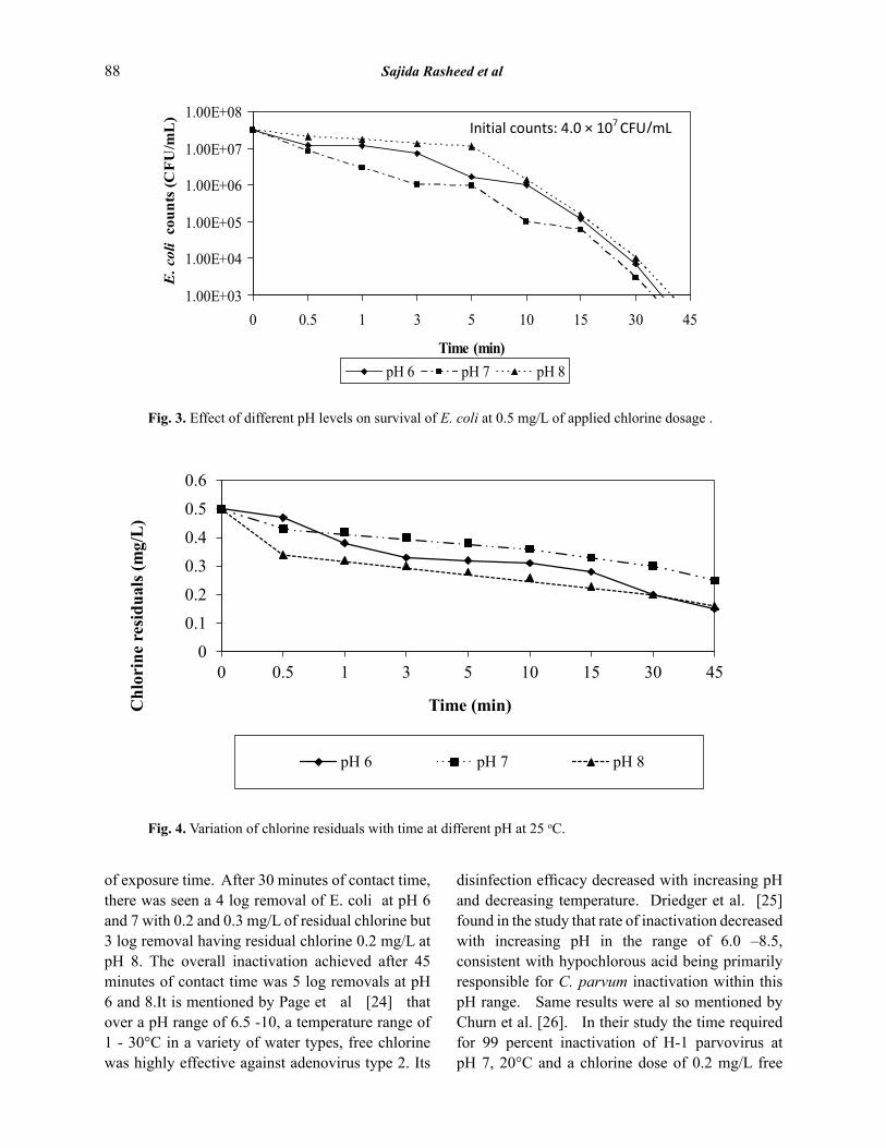
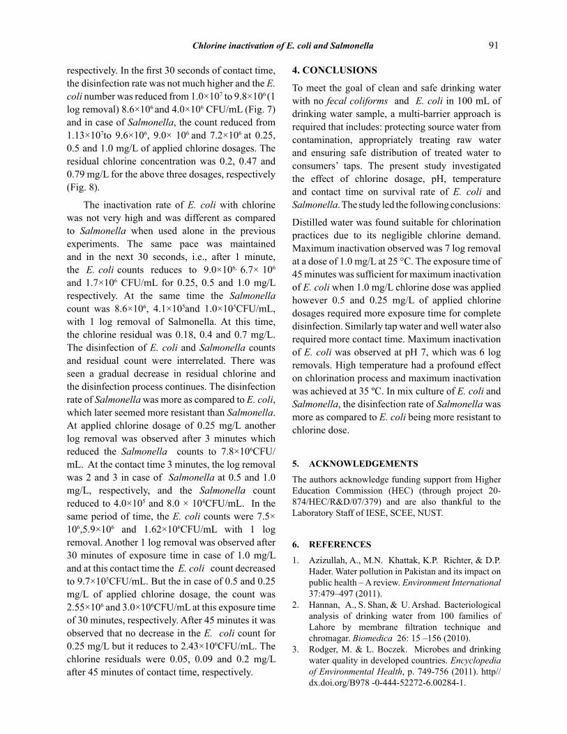
Fig. 3. Effect of different pH levels on survival of E. coli at 0.5 mg/L of applied chlorine dosage .
Fig. 4. Variation of chlorine residuals with time at different pH at 25 oC.
88 Sajida Rasheed et al
of exposure time. After 30 minutes of contact time, there was seen a 4 log removal of E. coli at pH 6 and 7 with 0.2 and 0.3 mg/L of residual chlorine but 3 log removal having residual chlorine 0.2 mg/L at pH 8. The overall inactivation achieved after 45 minutes of contact time was 5 log removals at pH 6 and 8.It is mentioned by Page et al [24] that over a pH range of 6.5 -10, a temperature range of 1 - 30°C in a variety of water types, free chlorine was highly effective against adenovirus type 2. Its
disinfection efficacy decreased with increasing pH and decreasing temperature. Driedger et al. [25] found in the study that rate of inactivation decreased with increasing pH in the range of 6.0 –8.5, consistent with hypochlorous acid being primarily responsible for C. parvum inactivation within this pH range. Same results were al so mentioned by Churn et al. [26]. In their study the time required for 99 percent inactivation of H-1 parvovirus at pH 7, 20°C and a chlorine dose of 0.2 mg/L free

Fig. 5. Survival of E. coli at 0.5 mg/L applied chlorine dosages in distilled water at various temperatures.
Fig. 6. Variation of chlorine dose with time at various temperatures.
Chlorine inactivation of E. coli and Salmonella 89
chlorine was 3.2 min.
3.3 Determination of Optimum Temperature for Maximum Disinfection of E. coli
From the results of previous set of experiments, it is evident that at pH 7, maximum inactivation of E. coli was resulted. Now in this set of experiments, the effect of temperature was studied selecting 0.5 mg/L applied chlorine dosage as used earlier and pH 7 as proved best in the previous experiments.
The initial count applied was 1.17×10⁷ CFU/mL at three different temperatures, viz. 15, 25 and 35ºC to observe the disinfection efficiency of chlorine. In the first 30 seconds of exposure time, the disinfection rate was evident and the E. coli counts reduced from 8.0× 10⁷ to 2.21×10⁶, 6.5×10⁶ and 5.7×10⁶ giving 1 log removal at 15, 25 and 35ºC, respectively, as shown in Fig. 5, depicting 35ºC as optimum among the three tested temperatures. At this time the residual chlorine concentration was

Fig. 7. Comparison of percent survival of E. coli and Salmonella in mix culture at 1.0 mg/L of applied chlorine dosage in distilled water.
Fig. 8. Variation of residual chlorine with time at 25ºC in mix at various chlorine doses.
90 Sajida Rasheed et al
determined as 0.49, 0.49 and 0.48 mg/L (Fig. 6). A decrease in residual chlorine was observed with time as E. coli number reduced depicting that more chlorine is being used for the removal of microbial count. The increase in temperature enhanced the disinfection efficiency of chlorine, i.e., pathogen inactivation effectiveness increased as water temperature rose as reported previously [21].
3.4 Effect of Chlorine on Mix Culture of E. coli and Salmonella
Beside monoculture of E. coli inactivation studies, mix culture of E. coli and Salmonella was also used to observe the disinfection behavior of chlorine in distilled water at25º C and pH 7. The initial counts after inoculation of pure culture of E. coli and Salmonella were 1.0×10⁷ and 1.13×10⁷CFU/mL,
Chlorine inactivation of E. coli and Salmonella 91
respectively. In the first 30 seconds of contact time, the disinfection rate was not much higher and the E. coli number was reduced from 1.0×10⁷ to 9.8×10⁶ (1 log removal) 8.6×10⁶ and 4.0×10⁶ CFU/mL (Fig. 7) and in case of Salmonella, the count reduced from 1.13×10⁷to 9.6×10⁶, 9.0× 10⁶ and 7.2×10⁶ at 0.25, 0.5 and 1.0 mg/L of applied chlorine dosages. The residual chlorine concentration was 0.2, 0.47 and 0.79 mg/L for the above three dosages, respectively (Fig. 8).
The inactivation rate of E. coli with chlorine was not very high and was different as compared to Salmonella when used alone in the previous experiments. The same pace was maintained and in the next 30 seconds, i.e., after 1 minute, the E. coli counts reduces to 9.0×10⁶, 6.7× 10⁶
and 1.7×10⁶ CFU/mL for 0.25, 0.5 and 1.0 mg/L respectively. At the same time the Salmonella count was 8.6×10⁶, 4.1×10⁵and 1.0×10⁵CFU/mL, with 1 log removal of Salmonella. At this time, the chlorine residual was 0.18, 0.4 and 0.7 mg/L. The disinfection of E. coli and Salmonella counts and residual count were interrelated. There was seen a gradual decrease in residual chlorine and the disinfection process continues. The disinfection rate of Salmonella was more as compared to E. coli, which later seemed more resistant than Salmonella. At applied chlorine dosage of 0.25 mg/L another log removal was observed after 3 minutes which reduced the Salmonella counts to 7.8×10⁶CFU/mL. At the contact time 3 minutes, the log removal was 2 and 3 in case of Salmonella at 0.5 and 1.0 mg/L, respectively, and the Salmonella count reduced to 4.0×10⁵ and 8.0 × 10⁴CFU/mL. In the same period of time, the E. coli counts were 7.5× 106,5.9×106 and 1.62×10⁶CFU/mL with 1 log removal. Another 1 log removal was observed after 30 minutes of exposure time in case of 1.0 mg/L and at this contact time the E. coli count decreased to 9.7×10⁵CFU/mL. But the in case of 0.5 and 0.25 mg/L of applied chlorine dosage, the count was 2.55×10⁶ and 3.0×10⁶CFU/mL at this exposure time of 30 minutes, respectively. After 45 minutes it was observed that no decrease in the E. coli count for 0.25 mg/L but it reduces to 2.43×10⁶CFU/mL. The chlorine residuals were 0.05, 0.09 and 0.2 mg/L after 45 minutes of contact time, respectively.
4. CONCLUSIONS
To meet the goal of clean and safe drinking water with no fecal coliforms and E. coli in 100 mL of drinking water sample, a multi-barrier approach is required that includes: protecting source water from contamination, appropriately treating raw water and ensuring safe distribution of treated water to consumers’ taps. The present study investigated the effect of chlorine dosage, pH, temperature and contact time on survival rate of E. coli and Salmonella. The study led the following conclusions:
Distilled water was found suitable for chlorination practices due to its negligible chlorine demand. Maximum inactivation observed was 7 log removal at a dose of 1.0 mg/L at 25 °C. The exposure time of 45 minutes was sufficient for maximum inactivation of E. coli when 1.0 mg/L chlorine dose was applied however 0.5 and 0.25 mg/L of applied chlorine dosages required more exposure time for complete disinfection. Similarly tap water and well water also required more contact time. Maximum inactivation of E. coli was observed at pH 7, which was 6 log removals. High temperature had a profound effect on chlorination process and maximum inactivation was achieved at 35 ºC. In mix culture of E. coli and Salmonella, the disinfection rate of Salmonella was more as compared to E. coli being more resistant to chlorine dose.
5. ACKNOWLEDGEMENTS
The authors acknowledge funding support from Higher Education Commission (HEC) (through project 20-874/HEC/R&D/07/379) and are also thankful to the Laboratory Staff of IESE, SCEE, NUST.
6. REFERENCES
1. Azizullah, A., M.N. Khattak, K.P. Richter, & D.P. Hader. Water pollution in Pakistan and its impact on public health – A review. Environment International 37:479–497 (2011).
2. Hannan, A., S. Shan, & U. Arshad. Bacteriological analysis of drinking water from 100 families of Lahore by membrane filtration technique and chromagar. Biomedica 26: 15 –156 (2010).
3. Rodger, M. & L. Boczek. Microbes and drinking water quality in developed countries. Encyclopedia of Environmental Health, p. 749-756 (2011). http//dx.doi.org/B978 -0-444-52272-6.00284-1.

92 Sajida Rasheed et al
4. Jones, D.L. Potential health risks associated with the persistence of Escherichia coli O157 in agricultural environments. Soil Use Management 15: 76–83 (1999).
5. Ram, S., P. Vajpayee, R. L. Singh & R. Shanker. Surface water of a perennial river exhibits multi-antimicrobial resistant shiga toxin and enterotoxin producing Escherichia coli. Ecotoxicology and Environmental Safety 72 (2): 490-495 (2009).
6. Hussain, I.A., T.S. Hussain, & Z. Sarwar. Microbial study of drinking water from Rawalakot and its surroundings. Online Journal of Biological Science 1 (4): 287-288 (2001).
7. Min, J. & A.J. Baeumner. Highly sensitive and specific detection of viable Escherichia coli in drinking water. Analytical Biochemistry 303 (2): 186 (2002).
8. Bej, A.K., R.J. Steffan, J. DiCesare , L. Haff, & R.M. Atlas. Detection of coliform bacteria in water by polimerase chain reaction and genes probes. Applied Environmental Microbiology 56:307 (1990).
9. Anwar, M.S., S. Lateef, & G. M. Siddiqui. Bacteriological quality of drinking water in Lahore. Biomedica 26: 66-69 (2010).
10. Schets, F.M., M. During, R. Italiaander, L. Heijnen, S.A. Rutjes, W.K.V. Zwaluw, & A.M.R. Husman. Escherichia coli O157:H7 in drinking water from private water supplies in the Netherlands. Water Research 39: 4485-4493 (2005) .
11. Berry, D.C. Xi, & L. Raskin .Microbial ecology of drinking water distribution systems. Current Opinion in Biotechnology 17: 297–302 (2006).
12. Fisher, I., G. Kastl, & A. Sathasivan. Evaluation of suitable chlorine bulk-decay models for water distribution systems. Water Research 45: 4896-4908 (2011).
13. Aisopou, A., I. Stoianov, & N.J.D. Graham. In-pipe water quality monitoring in water supply systems under steady and unsteady state flow conditions: A quantitative assessment. Water Research 46: 235 -246 (2012).
14. Robescu, D., N. Jivan, & D. Robescu. Chlorine decay in drinking water mains. Environment Engineering and Management Journal 7(6): 737-
741(2008). 15. Shang, C. & E. R. Blatchey. Chlorination of
pure bacterial culture in aqueous solution. Water Research. 35 (1): 244- 254 (2001).
16. Alam, S.M.N., G. Mostafa, & D.H. Bhuiyan. Prevalence of bacteria in the muscle of shrimp in processing plant. International Journal of Food Safety 5: 21-23 (2003).
17. Cappuccino, J.G. & N. Sherman. Microbiology: A Laboratory Manual, 4th ed. The Benjamin/Cummings Publishing Company (1996).
18. Wohlsen, T., J. Bates, G. Vesey, W.A. Robinson, & M. Katouli. Evaluation of the methods for enumerating coliforms bacteria from water samples using precise reference. Letters in Applied Microbiology (The Society for Applied Microbiology) 42: 350-356 (2006).
19. APHA. Standard Methods for the Examination of Water and Wastewater. American Public Health Association, Washington, DC (2005).
20. Massa, S., R. Armuzzi, M. Tosques, F. Canganella, & L.D. Trovatelli. Susceptibility to chlorine of Aeromonas hydrophila strains. Journal of Applied Microbiology 86 (1): 169-173 (1998).
21. US-EPA. EPA Office of Water: Alternative Disinfectants and Oxidants Guidance Manual. (EPA 815-R -99-014). Washington, DC (1999).
22. Gorchev, H.G. Chlorine in water disinfection. Pure and Applied Chemistry 68 (9): 1731 -1735 (1996).
23. Kenyon & F. Katheryn. Free Available Chlorine Disinfection Criteria for Fixed Army Installation Primary Drinking Water. Technical Report, 1974-1978. ADA114482. Defence Technical Information Centre (1981).
24. Page, M.A., J.L. Shisler, & B.J. Mariñas. Kinetics of adenovirus type 2 inactivation with free chlorine. Water Research 43: 2916 -2926 (2009).
25. Driedger, A.M., J.L. Rennecker, & B.J., Mariñas. Sequential inactivation of Cryptosporidium parvum oocysts with ozone and free chlorine. Water Research 34 (14): 3591-3597 (2000).
26. Churn, C.C., G.D. Boardman, & R.C Bates. The inactivation kinetics of H-1 parvovirus by chlorine. Water Research 18 (2): 195-203 (2003).

Research Article
Proceedings of the Pakistan Academy of Sciences: Pakistan Academy of SciencesB. Life and Environmental Sciences 53 (2): 93–102 (2016)Copyright © Pakistan Academy of SciencesISSN: 0377 - 2969 (print), 2306 - 1448 (online)
————————————————Received, April 2016; Accepted, June 2016*Corresponding Author: Ghulam Hussain; Email: [email protected]
Wastewater Characterization of Selected Industries in Quaid-e-Azam Industrial Estate: Treatment Options and
Impact on Groundwater Quality
Sajjad Haydar1, Ghulam Hussain1*, Husnain Haider2, and Attiq-ur-Rehman1
1Institute of Environmental Engineering & Research, University of Engineering & Technology, Lahore, Pakistan
2University of British Columbia, Vancouver, Canada
Abstract: This research was carried out to characterize the wastewater of major industries of Quaid-e-Azam Industrial Estate (QIE), to analyze effect of wastewater drain on groundwater quality in the area, and to suggest appropriate wastewater treatment option(s) for QIE. Composite wastewater samples were collected and analyzed for pH, temperature, biochemical oxygen demand (BOD), filtered BOD (F-BOD), chemical oxygen demand (COD), filtered COD (F-COD), total Kjeldahl nitrogen (N), total suspended solids (TSS), total dissolved solids (TDS), sulphates, chromium (Cr), lead (Pb), cadmium (Cd) and copper (Cu). Results showed that BOD, COD, TSS, TKN, Pb and Cd exceeded the limits of National Environmental Quality Standards Furthermore, groundwater samples were collected from selected tube wells in near vicinity of QIE and analyzed for pH, nitrates, total hardness, TDS, turbidity, sulphates, Pb, Cd, Cr and Cu. The results showed that groundwater contamination with Pb, Cd, and Cr due to unlined industrial drain.
Keywords: Industrial effluent, Quaid-e-Azam Industrial Estate, groundwater, BOD, COD, heavy metals, CETP, pollution load, pollution surcharge
1. INTRODUCTION
Industrialization leads to socio-economic uplift, especially in developing countries [1]. However, industrialization also leads to environment deterioration [2-3]. One of its productions is the industrial wastewater, inadequate and unscientific management of which has become the most critical problem in developing countries, resulting in the pollution of receiving water bodies [4-5]. It not only affects aquatic life but also has adverse impacts on public health [6].
In Pakistan, most of the industrial effluents are discharged into unlined surface drains without any treatment. Poor management, lack of planning and implementation of environment legislation worsened the situation than it was in past [7-9]. The wastewater generated by various industries has different characteristics depending upon type of raw material used and the processes involved
[10]. The wastewater usually contains suspended solids, heavy metals, organic matter, bases, acids and colouring compounds those could affect the quality of surface waters [11] and groundwater [12-14]. It can cause serious problems to aquatic flora and fauna and downstream water users. Presently, almost 3.4 million people die every year worldwide due to water borne diseases [15]. Cancer, diarrhea, hepatitis and different skin problems are the major illnesses that are evident as a result of groundwater contamination due to industrial effluent. Considering the gravity of the problem, there is an urgent need to treat industrial wastewater before discharging into receiving water bodies to ensure environmental protection [16].
The Quaid-e-Azam Industrial Estate (QIE) is one of the major planned Industrial Estates in Punjab. It spreads over an area of 565 acres (229 ha). It is located in the Southern part of Lahore on PECO
94 Sajjad Haydar et al
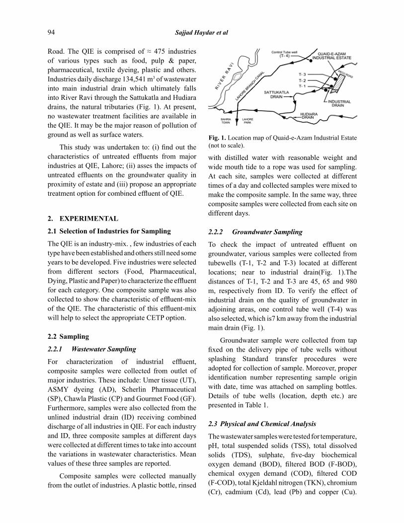
Road. The QIE is comprised of ≈ 475 industries of various types such as food, pulp & paper, pharmaceutical, textile dyeing, plastic and others. Industries daily discharge 134,541 m3 of wastewater into main industrial drain which ultimately falls into River Ravi through the Sattukatla and Hudiara drains, the natural tributaries (Fig. 1). At present, no wastewater treatment facilities are available in the QIE. It may be the major reason of pollution of ground as well as surface waters.
This study was undertaken to: (i) find out the characteristics of untreated effluents from major industries at QIE, Lahore; (ii) asses the impacts of untreated effluents on the groundwater quality in proximity of estate and (iii) propose an appropriate treatment option for combined effluent of QIE.
2. EXPERIMENTAL
2.1 Selection of Industries for Sampling
The QIE is an industry-mix. , few industries of each type have been established and others still need some years to be developed. Five industries were selected from different sectors (Food, Pharmaceutical, Dying, Plastic and Paper) to characterize the effluent for each category. One composite sample was also collected to show the characteristic of effluent-mix of the QIE. The characteristic of this effluent-mix will help to select the appropriate CETP option.
2.2 Sampling
2.2.1 Wastewater Sampling
For characterization of industrial effluent, composite samples were collected from outlet of major industries. These include: Umer tissue (UT), ASMY dyeing (AD), Scherlin Pharmaceutical (SP), Chawla Plastic (CP) and Gourmet Food (GF). Furthermore, samples were also collected from the unlined industrial drain (ID) receiving combined discharge of all industries in QIE. For each industry and ID, three composite samples at different days were collected at different times to take into account the variations in wastewater characteristics. Mean values of these three samples are reported.
Composite samples were collected manually from the outlet of industries. A plastic bottle, rinsed
Fig. 1. Location map of Quaid-e-Azam Industrial Estate (not to scale).
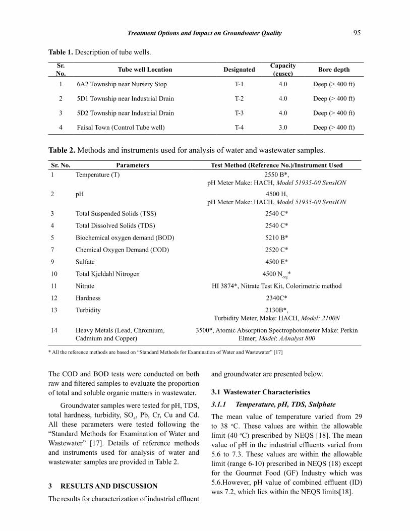
Fig. 2. TSS for the industrial wastewater samples.
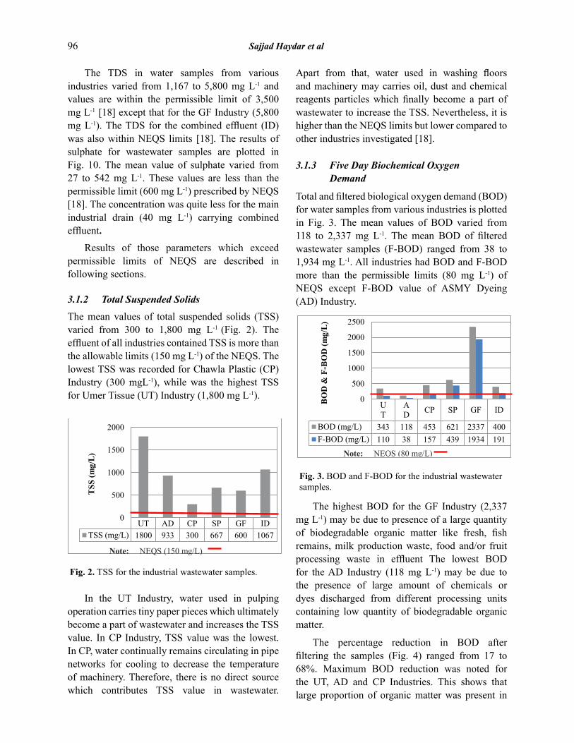
Fig. 3. BOD and F-BOD for the industrial wastewater samples.
UT AD CP SP GF IDTSS (mg/L) 1800 933 300 667 600 1067
0
500
1000
1500
2000
TSS
(mg/
L)
UT
AD CP SP GF ID
BOD (mg/L) 343 118 453 621 2337 400F-BOD (mg/L) 110 38 157 439 1934 191
0
500
1000
1500
2000
2500
BO
D &
F-B
OD
(mg/
L)
Note: NEQS (150 mg/L)
Note: NEQS (80 mg/L)
with distilled water with reasonable weight and wide mouth tide to a rope was used for sampling. At each site, samples were collected at different times of a day and collected samples were mixed to make the composite sample. In the same way, three composite samples were collected from each site on different days.
2.2.2 Groundwater Sampling
To check the impact of untreated effluent on groundwater, various samples were collected from tubewells (T-1, T-2 and T-3) located at different locations; near to industrial drain(Fig. 1).The distances of T-1, T-2 and T-3 are 45, 65 and 980 m, respectively from ID. To verify the effect of industrial drain on the quality of groundwater in adjoining areas, one control tube well (T-4) was also selected, which is7 km away from the industrial main drain (Fig. 1).
Groundwater sample were collected from tap fixed on the delivery pipe of tube wells without splashing Standard transfer procedures were adopted for collection of sample. Moreover, proper identification number representing sample origin with date, time was attached on sampling bottles. Details of tube wells (location, depth etc.) are presented in Table 1.
2.3 Physical and Chemical Analysis
The wastewater samples were tested for temperature, pH, total suspended solids (TSS), total dissolved solids (TDS), sulphate, five-day biochemical oxygen demand (BOD), filtered BOD (F-BOD), chemical oxygen demand (COD), filtered COD (F-COD), total Kjeldahl nitrogen (TKN), chromium (Cr), cadmium (Cd), lead (Pb) and copper (Cu).
Treatment Options and Impact on Groundwater Quality 95
The COD and BOD tests were conducted on both raw and filtered samples to evaluate the proportion of total and soluble organic matters in wastewater.
Groundwater samples were tested for pH, TDS, total hardness, turbidity, SO4, Pb, Cr, Cu and Cd. All these parameters were tested following the “Standard Methods for Examination of Water and Wastewater” [17]. Details of reference methods and instruments used for analysis of water and wastewater samples are provided in Table 2.
3 RESULTS AND DISCUSSION
The results for characterization of industrial effluent
and groundwater are presented below.
3.1 Wastewater Characteristics
3.1.1 Temperature, pH, TDS, Sulphate
The mean value of temperature varied from 29 to 38 oC. These values are within the allowable limit (40 oC) prescribed by NEQS [18]. The mean value of pH in the industrial effluents varied from 5.6 to 7.3. These values are within the allowable limit (range 6-10) prescribed in NEQS (18) except for the Gourmet Food (GF) Industry which was 5.6.However, pH value of combined effluent (ID) was 7.2, which lies within the NEQS limits[18].
Table 1. Description of tube wells.
Sr. No. Tube well Location Designated Capacity
(cusec) Bore depth
1 6A2 Township near Nursery Stop T-1 4.0 Deep (> 400 ft)
2 5D1 Township near Industrial Drain T-2 4.0 Deep (> 400 ft)
3 5D2 Township near Industrial Drain T-3 4.0 Deep (> 400 ft)
4 Faisal Town (Control Tube well) T-4 3.0 Deep (> 400 ft)
Table 2. Methods and instruments used for analysis of water and wastewater samples.
Sr. No. Parameters Test Method (Reference No.)/Instrument Used 1 Temperature (T) 2550 B*,
pH Meter Make: HACH, Model 51935-00 SensION
2 pH 4500 H, pH Meter Make: HACH, Model 51935-00 SensION
3 Total Suspended Solids (TSS) 2540 C*
4 Total Dissolved Solids (TDS) 2540 C*
5 Biochemical oxygen demand (BOD) 5210 B*
7 Chemical Oxygen Demand (COD) 2520 C*
9 Sulfate 4500 E*
10 Total Kjeldahl Nitrogen 4500 Norg*
11 Nitrate HI 3874*, Nitrate Test Kit, Colorimetric method
12 Hardness 2340C*
13 Turbidity 2130B*,Turbidity Meter, Make: HACH, Model: 2100N
14 Heavy Metals (Lead, Chromium, Cadmium and Copper)
3500*, Atomic Absorption Spectrophotometer Make: Perkin Elmer; Model: AAnalyst 800
* All the reference methods are based on “Standard Methods for Examination of Water and Wastewater” [17]
96 Sajjad Haydar et al
The TDS in water samples from various industries varied from 1,167 to 5,800 mg L-1 and values are within the permissible limit of 3,500 mg L-1 [18] except that for the GF Industry (5,800 mg L-1). The TDS for the combined effluent (ID) was also within NEQS limits [18]. The results of sulphate for wastewater samples are plotted in Fig. 10. The mean value of sulphate varied from 27 to 542 mg L-1. These values are less than the permissible limit (600 mg L-1) prescribed by NEQS [18]. The concentration was quite less for the main industrial drain (40 mg L-1) carrying combined effluent.
Results of those parameters which exceed permissible limits of NEQS are described in following sections.
3.1.2 Total Suspended Solids
The mean values of total suspended solids (TSS) varied from 300 to 1,800 mg L-1 (Fig. 2). The effluent of all industries contained TSS is more than the allowable limits (150 mg L-1) of the NEQS. The lowest TSS was recorded for Chawla Plastic (CP) Industry (300 mgL-1), while was the highest TSS for Umer Tissue (UT) Industry (1,800 mg L-1).
Apart from that, water used in washing floors and machinery may carries oil, dust and chemical reagents particles which finally become a part of wastewater to increase the TSS. Nevertheless, it is higher than the NEQS limits but lower compared to other industries investigated [18].
3.1.3 Five Day Biochemical Oxygen Demand
Total and filtered biological oxygen demand (BOD) for water samples from various industries is plotted in Fig. 3. The mean values of BOD varied from 118 to 2,337 mg L-1. The mean BOD of filtered wastewater samples (F-BOD) ranged from 38 to 1,934 mg L-1. All industries had BOD and F-BOD more than the permissible limits (80 mg L-1) of NEQS except F-BOD value of ASMY Dyeing (AD) Industry.
Fig. 1. Location map of Quaid-e-Azam Industrial Estate (not to scale).
Fig. 2. TSS for the industrial wastewater samples.
Fig. 3. BOD and F-BOD for the industrial wastewater samples.
UT AD CP SP GF IDTSS (mg/L) 1800 933 300 667 600 1067
0
500
1000
1500
2000
TSS
(mg/
L)
UT
AD CP SP GF ID
BOD (mg/L) 343 118 453 621 2337 400F-BOD (mg/L) 110 38 157 439 1934 191
0
500
1000
1500
2000
2500
BO
D &
F-B
OD
(mg/
L)
Note: NEQS (150 mg/L)
Note: NEQS (80 mg/L)
In the UT Industry, water used in pulping operation carries tiny paper pieces which ultimately become a part of wastewater and increases the TSS value. In CP Industry, TSS value was the lowest. In CP, water continually remains circulating in pipe networks for cooling to decrease the temperature of machinery. Therefore, there is no direct source which contributes TSS value in wastewater.
Fig. 1. Location map of Quaid-e-Azam Industrial Estate (not to scale).
Fig. 2. TSS for the industrial wastewater samples.
Fig. 3. BOD and F-BOD for the industrial wastewater samples.
UT AD CP SP GF IDTSS (mg/L) 1800 933 300 667 600 1067
0
500
1000
1500
2000
TSS
(mg/
L)
UT
AD CP SP GF ID
BOD (mg/L) 343 118 453 621 2337 400F-BOD (mg/L) 110 38 157 439 1934 191
0
500
1000
1500
2000
2500B
OD
& F
-BO
D (m
g/L
)
Note: NEQS (150 mg/L)
Note: NEQS (80 mg/L)
The highest BOD for the GF Industry (2,337 mg L-1) may be due to presence of a large quantity of biodegradable organic matter like fresh, fish remains, milk production waste, food and/or fruit processing waste in effluent The lowest BOD for the AD Industry (118 mg L-1) may be due to the presence of large amount of chemicals or dyes discharged from different processing units containing low quantity of biodegradable organic matter.
The percentage reduction in BOD after filtering the samples (Fig. 4) ranged from 17 to 68%. Maximum BOD reduction was noted for the UT, AD and CP Industries. This shows that large proportion of organic matter was present in

Treatment Options and Impact on Groundwater Quality 97
Fig. 7. TKN for the industrial wastewater samples.
Fig. 8. Lead in the industrial wastewater samples.
Fig. 9. Chromium in the industrial wastewater samples.
UT AD CP SP GF IDTKN (mg/L) 10 17 1 5 17 25
05
1015202530
TK
N (m
g/L
)
UT AD CP SP GF IDPb (mg/L) 1.43 1.35 2.38 1.79 0.04 1.17
0.00
0.50
1.00
1.50
2.00
2.50
Pb (m
g/L
)
UT AD CP SP GF IDCr (mg/L) 0.88 0.24 0.79 0.42 0.02 0.96
0.00
0.20
0.40
0.60
0.80
1.00
1.20
Cr
(mg/
L)
Note: IFC Guideline (10 mg/L)
Note: NEQS (0.5 mg/L)
Note: NEQS (1 mg/L)
particulate form that could be removed in primary sedimentation step of treatment. However, for the GF Industry, the reduction was only 17% indicating that most of the organic matter is in dissolved form and an extensive biological treatment is required.
3.1.4 Chemical Oxygen Demand
Total and filtered chemical oxygen demand (COD) for all the samples are plotted in Fig. 5. The mean COD varied from 323 to 4,867 mg L-1. Furthermore, mean COD for the filtered wastewater samples (F-COD) ranged from 120 to 3,600 mgL-1. All the industries had COD and F-COD more than the permissible limits (150mg L-1) of the NEQS except F-COD value of ASMY Dyeing Industry.
oxygen to oxidize it. The lowest COD was for the AD Industry (323 mg L-1). The decrease in COD after filtering varied from 26 to 69%. After filtration, of the decrease in COD is plotted against each industry in Fig. 6. The maximum removal of COD was for the UT wastewater (69%) while the GF Industry experienced minimum removal (26%). The reasons appear the same as stated above for BOD.
3.1.5 Total Kjeldahl Nitrogen (TKN)
The mean values of total Kjeldahl nitrogen (TKN) varied from 1 to 25 mg L-1 for effluent samples (Fig. 7). These values are more than the permissible limit (10mg/-1) provided by the IFC Guideline [19] except for the GF, AD industry and the ID. The high values of TKN at GF and AD Industry seem due to high usage of nitrogenous compounds as raw materials. These nitrogenous compounds are present in food preservatives [20] which come out as organic nitrogen pollutants in industrial effluent.
Fig. 4. Percentage reduction of BOD after filtration.
Fig. 5. COD and F-COD for the industrial wastewater samples.
Fig. 6. Percentage reduction of COD after filtration.
UT AD CP SP GF ID% Red. 68% 67% 65% 29% 17% 52%
0%
20%
40%
60%
80%
100%%
age
Red
uctio
n of
B
OD
aft
er F
ilter
atio
n
UT
AD CP SP GF ID
COD (mg/L) 973 323 1347 1947 4867 1007F-COD (mg/L) 300 120 660 1340 3600 360
0
1000
2000
3000
4000
5000
CO
D &
F-C
OD
(mg/
L)
UT AD CP SP GF ID% Red. 69% 63% 51% 31% 26% 64%
0%
20%
40%
60%
80%
100%
% a
ge R
educ
tion
of
CO
D a
fter
Filt
erat
ion
Note: NEQS (150mg/L)
Fig. 4. Percentage reduction of BOD after filtration.
Fig. 5. COD and F-COD for the industrial wastewater samples.
Fig. 6. Percentage reduction of COD after filtration.
UT AD CP SP GF ID% Red. 68% 67% 65% 29% 17% 52%
0%
20%
40%
60%
80%
100%
% a
ge R
educ
tion
of
BO
D a
fter
Filt
erat
ion
UT
AD CP SP GF ID
COD (mg/L) 973 323 1347 1947 4867 1007F-COD (mg/L) 300 120 660 1340 3600 360
0
1000
2000
3000
4000
5000
CO
D &
F-C
OD
(mg/
L)
UT AD CP SP GF ID% Red. 69% 63% 51% 31% 26% 64%
0%
20%
40%
60%
80%
100%
% a
ge R
educ
tion
of
CO
D a
fter
Filt
erat
ion
Note: NEQS (150mg/L)
The highest COD for the GF Industry (4,867 mgL-1) could be due to presence of a large quantity of high organic load that requires more dissolved
Fig. 4. Percentage reduction of BOD after filtration.
Fig. 5. COD and F-COD for the industrial wastewater samples.
Fig. 6. Percentage reduction of COD after filtration.
UT AD CP SP GF ID% Red. 68% 67% 65% 29% 17% 52%
0%
20%
40%
60%
80%
100%
% a
ge R
educ
tion
of
BO
D a
fter
Filt
erat
ion
UT
AD CP SP GF ID
COD (mg/L) 973 323 1347 1947 4867 1007F-COD (mg/L) 300 120 660 1340 3600 360
0
1000
2000
3000
4000
5000
CO
D &
F-C
OD
(mg/
L)
UT AD CP SP GF ID% Red. 69% 63% 51% 31% 26% 64%
0%
20%
40%
60%
80%
100%
% a
ge R
educ
tion
of
CO
D a
fter
Filt
erat
ion
Note: NEQS (150mg/L)
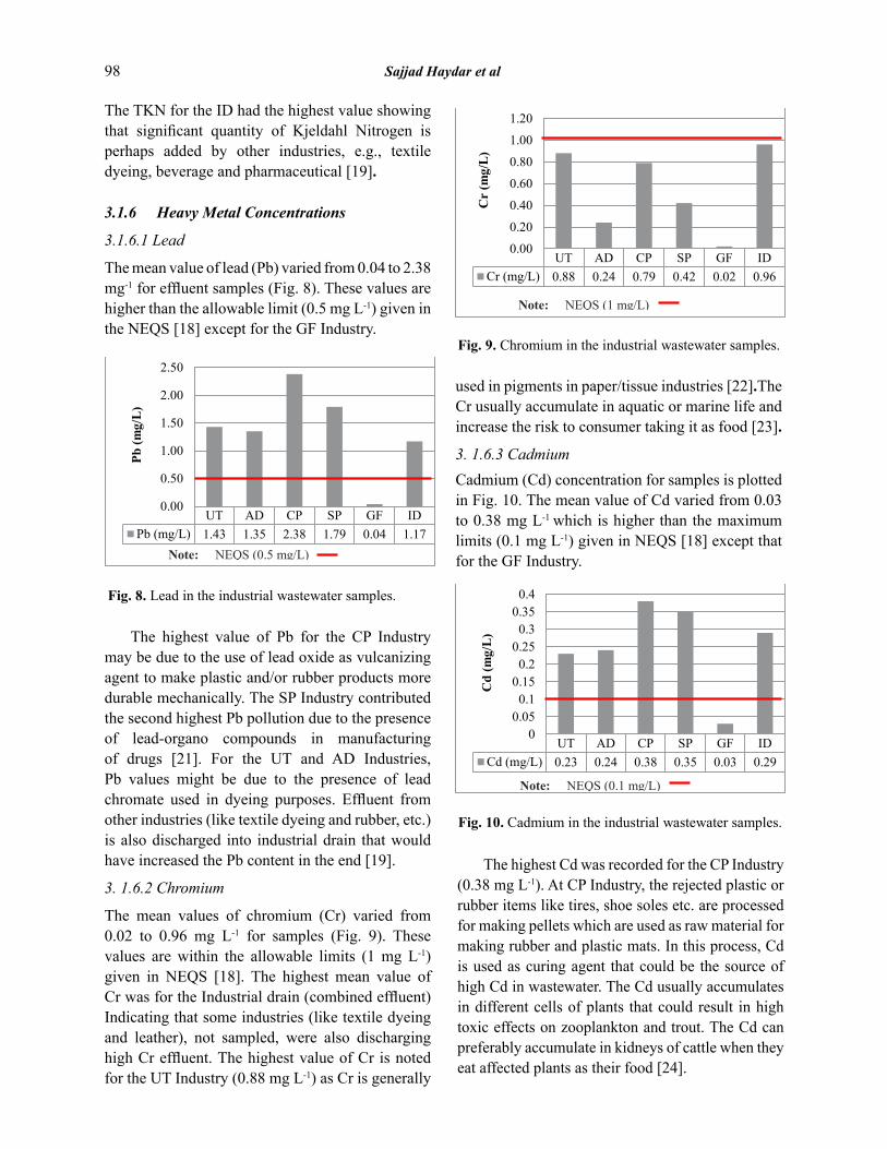
98 Sajjad Haydar et al
The TKN for the ID had the highest value showing that significant quantity of Kjeldahl Nitrogen is perhaps added by other industries, e.g., textile dyeing, beverage and pharmaceutical [19].
3.1.6 Heavy Metal Concentrations
3.1.6.1 Lead
The mean value of lead (Pb) varied from 0.04 to 2.38 mg-1 for effluent samples (Fig. 8). These values are higher than the allowable limit (0.5 mg L-1) given in the NEQS [18] except for the GF Industry.
Fig. 7. TKN for the industrial wastewater samples.
Fig. 8. Lead in the industrial wastewater samples.
Fig. 9. Chromium in the industrial wastewater samples.
UT AD CP SP GF IDTKN (mg/L) 10 17 1 5 17 25
05
1015202530
TK
N (m
g/L
)
UT AD CP SP GF IDPb (mg/L) 1.43 1.35 2.38 1.79 0.04 1.17
0.00
0.50
1.00
1.50
2.00
2.50
Pb (m
g/L
)
UT AD CP SP GF IDCr (mg/L) 0.88 0.24 0.79 0.42 0.02 0.96
0.00
0.20
0.40
0.60
0.80
1.00
1.20
Cr
(mg/
L)
Note: IFC Guideline (10 mg/L)
Note: NEQS (0.5 mg/L)
Note: NEQS (1 mg/L)
The highest value of Pb for the CP Industry may be due to the use of lead oxide as vulcanizing agent to make plastic and/or rubber products more durable mechanically. The SP Industry contributed the second highest Pb pollution due to the presence of lead-organo compounds in manufacturing of drugs [21]. For the UT and AD Industries, Pb values might be due to the presence of lead chromate used in dyeing purposes. Effluent from other industries (like textile dyeing and rubber, etc.) is also discharged into industrial drain that would have increased the Pb content in the end [19].
3. 1.6.2 Chromium
The mean values of chromium (Cr) varied from 0.02 to 0.96 mg L-1 for samples (Fig. 9). These values are within the allowable limits (1 mg L-1) given in NEQS [18]. The highest mean value of Cr was for the Industrial drain (combined effluent) Indicating that some industries (like textile dyeing and leather), not sampled, were also discharging high Cr effluent. The highest value of Cr is noted for the UT Industry (0.88 mg L-1) as Cr is generally
Fig. 7. TKN for the industrial wastewater samples.
Fig. 8. Lead in the industrial wastewater samples.
Fig. 9. Chromium in the industrial wastewater samples.
UT AD CP SP GF IDTKN (mg/L) 10 17 1 5 17 25
05
1015202530
TK
N (m
g/L
)
UT AD CP SP GF IDPb (mg/L) 1.43 1.35 2.38 1.79 0.04 1.17
0.00
0.50
1.00
1.50
2.00
2.50
Pb (m
g/L
)
UT AD CP SP GF IDCr (mg/L) 0.88 0.24 0.79 0.42 0.02 0.96
0.00
0.20
0.40
0.60
0.80
1.00
1.20
Cr
(mg/
L)
Note: IFC Guideline (10 mg/L)
Note: NEQS (0.5 mg/L)
Note: NEQS (1 mg/L)
used in pigments in paper/tissue industries [22].The Cr usually accumulate in aquatic or marine life and increase the risk to consumer taking it as food [23].
3. 1.6.3 CadmiumCadmium (Cd) concentration for samples is plotted in Fig. 10. The mean value of Cd varied from 0.03 to 0.38 mg L-1 which is higher than the maximum limits (0.1 mg L-1) given in NEQS [18] except that for the GF Industry.
Fig. 10. Cadmium in the industrial wastewater samples.
Fig. 11. Copper in the industrial wastewater samples.
Fig. 12. Lead in groundwater samples.
UT AD CP SP GF IDCd (mg/L) 0.23 0.24 0.38 0.35 0.03 0.29
00.050.1
0.150.2
0.250.3
0.350.4
Cd
(mg/
L)
UT AD CP SP GF IDCu (mg/L) 0.06 0.03 0.06 0.03 0.01 0.02
0.00
0.20
0.40
0.60
0.80
1.00
1.20
Cu
(mg/
L)
T-1 T-2 T-3 T-4Pb (mg/L) 1.17 1.56 1.56 0.008
0.000.200.400.600.801.001.201.401.601.80
Pb (m
g/L
)
Note: NEQS (0.1 mg/L)
Note: NEQS (1 mg/L)
Note: NDWQS (0.05 mg/L)
The highest Cd was recorded for the CP Industry (0.38 mg L-1). At CP Industry, the rejected plastic or rubber items like tires, shoe soles etc. are processed for making pellets which are used as raw material for making rubber and plastic mats. In this process, Cd is used as curing agent that could be the source of high Cd in wastewater. The Cd usually accumulates in different cells of plants that could result in high toxic effects on zooplankton and trout. The Cd can preferably accumulate in kidneys of cattle when they eat affected plants as their food [24].

Treatment Options and Impact on Groundwater Quality 99
3. 1.6.4 CopperThe mean value of copper (Cu) varied from 0.01 to 0.06 mg L-1 for samples (Fig. 11) and are within the allowable limits (1 mgL-1) given in NEQS [18]. The highest value was recorded the CP (0.06 mgL-1), UT (0.06 mg L-1) and GF (0.06 mg L-1) Industries. The Cu is generally discharge from those industries where it is used in electrical gears, roofing, plumbing and heat exchangers. This element is essential nutrient and is component for the growth of animals and plants. Copper is an essential substance to human life, but in high doses, it can cause anemia, liver and kidney damage, and stomach and intestinal irritation [23].
the collected samples was less than the detection limit (10 mgL-1). The allowable limit for nitrates is 50 mg L-1 in NDWQS [25].
Results of heavy metals in ground water samples are discussed in details in following sections.
3.2.2 Heavy metals concentration
3.2.2.1. Lead
The mean concentration of Pb varied from1.17 to 1.56 mg L-1 for groundwater (Fig. 12). These values are more than the allowable limit (0.05 mg L-1) provided by NDWQS (2010). The higher Pb values in groundwater might be due to the nearby flowing industrial drain having wastewater with high lead concentrations. The lead concentration for T-4 (0.008 mgL-1) is within the permissible limits of NDWQS (2010). This shows the adverse effect of unlined industrial drain on the groundwater quality of nearby tube wells. Similar results were reported for contamination of lead in groundwater due to the intrusion of wastewater from Hudiara drain [27]. Leaching of Pb into groundwater is possible, under favorable conditions [28].
Fig. 10. Cadmium in the industrial wastewater samples.
Fig. 11. Copper in the industrial wastewater samples.
Fig. 12. Lead in groundwater samples.
UT AD CP SP GF IDCd (mg/L) 0.23 0.24 0.38 0.35 0.03 0.29
00.050.1
0.150.2
0.250.3
0.350.4
Cd
(mg/
L)
UT AD CP SP GF IDCu (mg/L) 0.06 0.03 0.06 0.03 0.01 0.02
0.00
0.20
0.40
0.60
0.80
1.00
1.20
Cu
(mg/
L)
T-1 T-2 T-3 T-4Pb (mg/L) 1.17 1.56 1.56 0.008
0.000.200.400.600.801.001.201.401.601.80
Pb (m
g/L
)
Note: NEQS (0.1 mg/L)
Note: NEQS (1 mg/L)
Note: NDWQS (0.05 mg/L)
3.2 Effect of Untreated Wastewater Unlined Drain on Groundwater Quality
3.2.1 pH, Total Hardness, TDS, Sulphate, Turbidity, Nitrates The mean pH value for groundwater samples varied from 7.2 to 7.5 and are within allowable limit (6.5–8.5) for drinking water given in NDWQS[25].The mean values of total hardness varied from 45 to 63 mg L-1 as CaCO3 and are within the permissible limit (500 mg L-1 as CaCO3) prescribed by NDWQS [25].The mean TDS varied from 550 to 567 mg L-1 for groundwater samples which are within allowable limit (1,000 mg L-1) ofNDWQS[25].The mean sulphates varied from 48 to 49 mg/L-1 for groundwater samples. These values are within allowable limit (500 mg L-1) provided by WHO guidelines [26]. The turbidity varied from 0.6 to 1.2 NTU for groundwater. These values were within the allowable limits (5 NTU) prescribed in NDWQS (2010).The mean values of nitrates for all
Fig. 10. Cadmium in the industrial wastewater samples.
Fig. 11. Copper in the industrial wastewater samples.
Fig. 12. Lead in groundwater samples.
UT AD CP SP GF IDCd (mg/L) 0.23 0.24 0.38 0.35 0.03 0.29
00.050.1
0.150.2
0.250.3
0.350.4
Cd
(mg/
L)
UT AD CP SP GF IDCu (mg/L) 0.06 0.03 0.06 0.03 0.01 0.02
0.00
0.20
0.40
0.60
0.80
1.00
1.20
Cu
(mg/
L)
T-1 T-2 T-3 T-4Pb (mg/L) 1.17 1.56 1.56 0.008
0.000.200.400.600.801.001.201.401.601.80
Pb (m
g/L
)
Note: NEQS (0.1 mg/L)
Note: NEQS (1 mg/L)
Note: NDWQS (0.05 mg/L)
The high concentration of Pb in groundwater creates numerous problems for children and adults like decrease in IQ level, increase in risk of hypertension during pregnancy, arterial disease, delay puberty in males or females and affect the central nervous system [24].
3.2.2.2. Chromium
The Cr varied from 0.27 to 0.39 mg L-1 for groundwater (Fig. 13). These values are higher
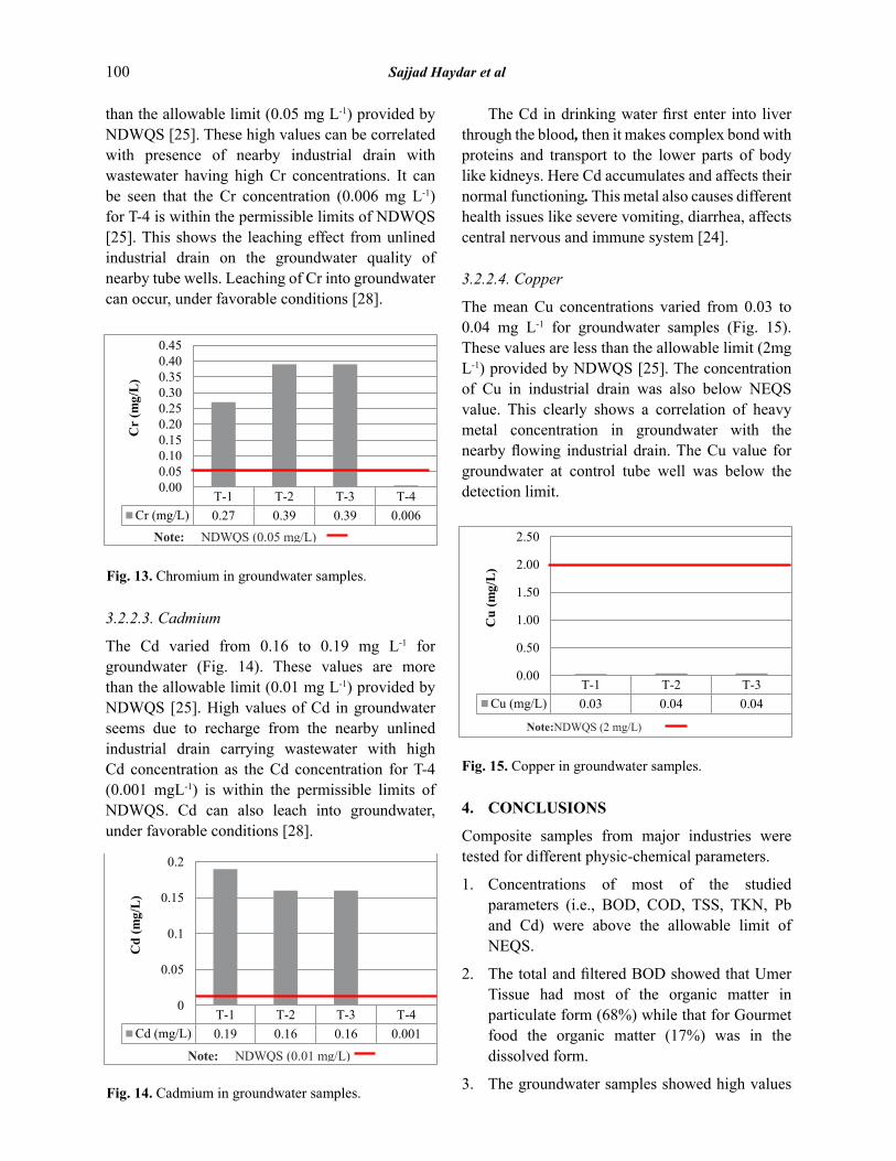
100 Sajjad Haydar et al
than the allowable limit (0.05 mg L-1) provided by NDWQS [25]. These high values can be correlated with presence of nearby industrial drain with wastewater having high Cr concentrations. It can be seen that the Cr concentration (0.006 mg L-1) for T-4 is within the permissible limits of NDWQS [25]. This shows the leaching effect from unlined industrial drain on the groundwater quality of nearby tube wells. Leaching of Cr into groundwater can occur, under favorable conditions [28].
The Cd in drinking water first enter into liver through the blood, then it makes complex bond with proteins and transport to the lower parts of body like kidneys. Here Cd accumulates and affects their normal functioning. This metal also causes different health issues like severe vomiting, diarrhea, affects central nervous and immune system [24].
3.2.2.4. Copper
The mean Cu concentrations varied from 0.03 to 0.04 mg L-1 for groundwater samples (Fig. 15). These values are less than the allowable limit (2mg L-1) provided by NDWQS [25]. The concentration of Cu in industrial drain was also below NEQS value. This clearly shows a correlation of heavy metal concentration in groundwater with the nearby flowing industrial drain. The Cu value for groundwater at control tube well was below the detection limit.
Fig. 13. Chromium in groundwater samples.
Fig. 14. Cadmium in groundwater samples.
Fig. 15. Copper in groundwater samples.
T-1 T-2 T-3 T-4Cr (mg/L) 0.27 0.39 0.39 0.006
0.000.050.100.150.200.250.300.350.400.45
Cr
(mg/
L)
T-1 T-2 T-3 T-4Cd (mg/L) 0.19 0.16 0.16 0.001
0
0.05
0.1
0.15
0.2
Cd
(mg/
L)
T-1 T-2 T-3Cu (mg/L) 0.03 0.04 0.04
0.00
0.50
1.00
1.50
2.00
2.50
Cu
(mg/
L)
Note: NDWQS (0.05 mg/L)
Note: NDWQS (0.01 mg/L)
Note:NDWQS (2 mg/L)
3.2.2.3. Cadmium
The Cd varied from 0.16 to 0.19 mg L-1 for groundwater (Fig. 14). These values are more than the allowable limit (0.01 mg L-1) provided by NDWQS [25]. High values of Cd in groundwater seems due to recharge from the nearby unlined industrial drain carrying wastewater with high Cd concentration as the Cd concentration for T-4 (0.001 mgL-1) is within the permissible limits of NDWQS. Cd can also leach into groundwater, under favorable conditions [28].
Fig. 13. Chromium in groundwater samples.
Fig. 14. Cadmium in groundwater samples.
Fig. 15. Copper in groundwater samples.
T-1 T-2 T-3 T-4Cr (mg/L) 0.27 0.39 0.39 0.006
0.000.050.100.150.200.250.300.350.400.45
Cr
(mg/
L)
T-1 T-2 T-3 T-4Cd (mg/L) 0.19 0.16 0.16 0.001
0
0.05
0.1
0.15
0.2
Cd
(mg/
L)
T-1 T-2 T-3Cu (mg/L) 0.03 0.04 0.04
0.00
0.50
1.00
1.50
2.00
2.50
Cu
(mg/
L)
Note: NDWQS (0.05 mg/L)
Note: NDWQS (0.01 mg/L)
Note:NDWQS (2 mg/L)
4. CONCLUSIONS
Composite samples from major industries were tested for different physic-chemical parameters.
1. Concentrations of most of the studied parameters (i.e., BOD, COD, TSS, TKN, Pb and Cd) were above the allowable limit of NEQS.
2. The total and filtered BOD showed that Umer Tissue had most of the organic matter in particulate form (68%) while that for Gourmet food the organic matter (17%) was in the dissolved form.
3. The groundwater samples showed high values
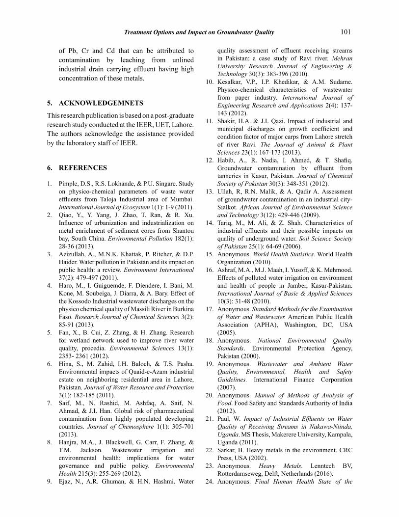
Treatment Options and Impact on Groundwater Quality 101
of Pb, Cr and Cd that can be attributed to contamination by leaching from unlined industrial drain carrying effluent having high concentration of these metals.
5. ACKNOWLEDGEMNETS
This research publication is based on a post-graduate research study conducted at the IEER, UET, Lahore. The authors acknowledge the assistance provided by the laboratory staff of IEER.
6. REFERENCES
1. Pimple, D.S., R.S. Lokhande, & P.U. Singare. Study on physico-chemical parameters of waste water effluents from Taloja Industrial area of Mumbai. International Journal of Ecosystem 1(1): 1-9 (2011).
2. Qiao, Y., Y. Yang, J. Zhao, T. Ran, & R. Xu. Influence of urbanization and industrialization on metal enrichment of sediment cores from Shantou bay, South China. Environmental Pollution 182(1): 28-36 (2013).
3. Azizullah, A., M.N.K. Khattak, P. Ritcher, & D.P. Haider. Water pollution in Pakistan and its impact on public health: a review. Environment International 37(2): 479-497 (2011).
4. Haro, M., I. Guiguemde, F. Diendere, I. Bani, M. Kone, M. Soubeiga, J. Diarra, & A. Bary. Effect of the Kossodo Industrial wastewater discharges on the physico chemical quality of Massili River in Burkina Faso. Research Journal of Chemical Sciences 3(2): 85-91 (2013).
5. Fan, X., B. Cui, Z. Zhang, & H. Zhang. Research for wetland network used to improve river water quality, procedia. Environmental Sciences 13(1): 2353- 2361 (2012).
6. Hina, S., M. Zahid, I.H. Baloch, & T.S. Pasha. Environmental impacts of Quaid-e-Azam industrial estate on neighboring residential area in Lahore, Pakistan. Journal of Water Resource and Protection 3(1): 182-185 (2011).
7. Saif, M., N. Rashid, M. Ashfaq, A. Saif, N. Ahmad, & J.I. Han. Global risk of pharmaceutical contamination from highly populated developing countries. Journal of Chemosphere 1(1): 305-701 (2013).
8. Hanjra, M.A., J. Blackwell, G. Carr, F. Zhang, & T.M. Jackson. Wastewater irrigation and environmental health: implications for water governance and public policy. Environmental Health 215(3): 255-269 (2012).
9. Ejaz, N., A.R. Ghuman, & H.N. Hashmi. Water
quality assessment of effluent receiving streams in Pakistan: a case study of Ravi river. Mehran University Research Journal of Engineering & Technology 30(3): 383-396 (2010).
10. Kesalkar, V.P., I.P. Khedikar, & A.M. Sudame. Physico-chemical characteristics of wastewater from paper industry. International Journal of Engineering Research and Applications 2(4): 137-143 (2012).
11. Shakir, H.A. & J.I. Qazi. Impact of industrial and municipal discharges on growth coefficient and condition factor of major carps from Lahore stretch of river Ravi. The Journal of Animal & Plant Sciences 23(1): 167-173 (2013).
12. Habib, A., R. Nadia, I. Ahmed, & T. Shafiq. Groundwater contamination by effluent from tanneries in Kasur, Pakistan. Journal of Chemical Society of Pakistan 30(3): 348-351 (2012).
13. Ullah, R, R.N. Malik, & A. Qadir A. Assessment of groundwater contamination in an industrial city-Sialkot. African Journal of Environmental Science and Technology 3(12): 429-446 (2009).
14. Tariq, M., M. Ali, & Z. Shah. Characteristics of industrial effluents and their possible impacts on quality of underground water. Soil Science Society of Pakistan 25(1): 64-69 (2006).
15. Anonymous. World Health Statistics. World Health Organization (2010).
16. Ashraf, M.A., M.J. Maah, I. Yusoff, & K. Mehmood. Effects of polluted water irrigation on environment and health of people in Jamber, Kasur-Pakistan. International Journal of Basic & Applied Sciences 10(3): 31-48 (2010).
17. Anonymous. Standard Methods for the Examination of Water and Wastewater. American Public Health Association (APHA), Washington, DC, USA (2005).
18. Anonymous. National Environmental Quality Standards. Environmental Protection Agency, Pakistan (2000).
19. Anonymous. Wastewater and Ambient Water Quality, Environmental, Health and Safety Guidelines. International Finance Corporation (2007).
20. Anonymous. Manual of Methods of Analysis of Food. Food Safety and Standards Authority of India (2012).
21. Paul, W. Impact of Industrial Effluents on Water Quality of Receiving Streams in Nakawa-Ntinda, Uganda. MS Thesis, Makerere University, Kampala, Uganda (2011).
22. Sarkar, B. Heavy metals in the environment. CRC Press, USA (2002).
23. Anonymous. Heavy Metals. Lenntech BV, Rotterdamseweg, Delft, Netherlands (2016).
24. Anonymous. Final Human Health State of the

102 Sajjad Haydar et al
Science Report on Heavy Metals. Ministry of Health-Canada 2(1): 55-68 (2013).
25. Anonymous. National Standards for Drinking Water Quality. Environmental Protection Agency, Pakistan (2010).
26. Anonymous. Guidelines for Drinking-Water Quality: Recommendations. World Health Organization (2004).
27. Haydar, S., H. Haider, O. Nadeem, G. Hussain, I.
Jalees, & A. Qadeer. Effect of Hudiara drain on the quality of groundwater in the housing schemes of Lahore. Journal of Faculty of Engineering & Technology. 21(2): 119-134 (2014).
28. McLean, J.E., & B.E. Bledsoe. Ground water issue: behavior of metals in soil. EPA Environmental Assessment Source Book No. EPA/540/S92/018) (1996).

Research Article
Proceedings of the Pakistan Academy of Sciences: Pakistan Academy of SciencesB. Life and Environmental Sciences 53 (2): 103–109 (2016)Copyright © Pakistan Academy of SciencesISSN: 0377 - 2969 (print), 2306 - 1448 (online)
————————————————Received, April 2016; Accepted, June 2016*Corresponding author: Abdul Basit Khan; Email: [email protected]
Microbiological Evaluation of Raw Meat Products Available in Local Markets of Karachi, Pakistan
AyeshaZafar,ErumAhmed,HafizaWajiha,andAbdulBasitKhan*
Department of Microbiology, Jinnah University for Women,5-C Nazimabad, Karachi, Pakistan
Abstract: Contaminated food products have been reported to be responsible for numerous food borne diseases all around the world. Microbial contaminants have been shown to be present in a wide variety of food products, especially in raw meat. For this reason, their isolation and detection in food is crucial for the safety of public health. The purpose of this research was to evaluate the microbiological quality of different meat samples including chicken, mutton and beef. Thirty (30) meat samples were purchased from different local meat retailer shops in Karachi. These samples were analyzed for their total aerobic count, total coliform count, fecal coliforms and Salmonellae according to standard methods. Examination of meat samples revealed that almost all samples were unfit for human consumption due to the presence of high aerobic count, coliforms, fecal coliforms and Salmonella spp. The average aerobic count log10cfu/g of chicken, mutton and beef samples was 6.67, 6.38 and 7.05 respectively. Out of 30 samples, 29 were heavily contaminated with coliforms and among them 26 were positive for fecal coliforms. The results also showed that 13 out of 30 meat samples were positive for Salmonella using conventional and PCR methods. The microbiological quality of meat was associated with handling and processing in unhygienic conditions. It was concluded that the food industry and regulatory authorities concerning food safety should take better control measures to improve food hygiene and prevent the contamination of food to maintain public health status and also control the rate of incidence of food borne diseases.
Keywords: Raw meat, total aerobic count, coliforms, Salmonella
1. INTRODUCTION
Food borne diseases are the major cause of mortality and infections especially in the developing countries. A variety of pathogenic microorganisms including bacteria, viruses, protozoans, parasites are involved in number of severe outbreaks worldwide. According to an estimate, 600 million food-related infections occurred in 2010 alone with 420,000 deaths [1]. In 2013, 818 food borne outbreaks were reported in USA, which resulted in 13,360 illnesses, 1,062 hospitalizations along with 16 deaths, and 14 foods recalls [2]. Outbreaks caused by Salmonella; a food borne pathogen, increased 39% from 2012 (113) to 2013 (157). Outbreak associated hospitalizations caused by Salmonella spp. increased 38% from 2012 (454) to
2013 (628) [2]. In addition, several reports related to contaminated food products being imported or exported have further complex the situation of food safety and public health worldwide. The global economy links local markets to international markets on an unparalleled scale, which results in unrestricted transportation of contaminated food involving numerous countries in Asia, Europe, and Latin America [3].
Meat and meat products are among the most important edible commodities originating from cattle, poultry and fishes. They serve as an ideal medium for the growth of many organisms due to increased water activity, favorable pH and higher concentrations of proteins, minerals, growth factors, fermentable carbohydrates, etc.
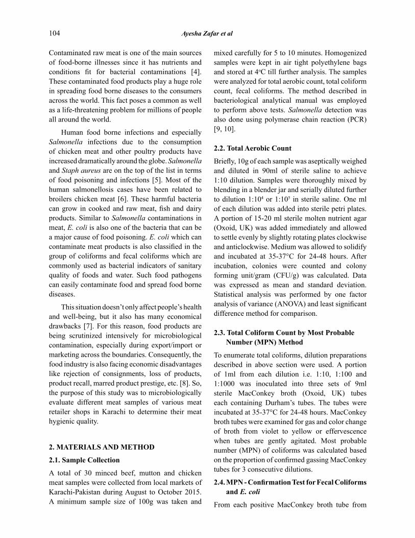
104 Ayesha Zafar et al
Contaminated raw meat is one of the main sources of food-borne illnesses since it has nutrients and conditions fit for bacterial contaminations [4]. These contaminated food products play a huge role in spreading food borne diseases to the consumers across the world. This fact poses a common as well as a life-threatening problem for millions of people all around the world.
Human food borne infections and especially Salmonella infections due to the consumption of chicken meat and other poultry products have increased dramatically around the globe. Salmonella and Staph aureus are on the top of the list in terms of food poisoning and infections [5]. Most of the human salmonellosis cases have been related to broilers chicken meat [6]. These harmful bacteria can grow in cooked and raw meat, fish and dairy products. Similar to Salmonella contaminations in meat, E. coli is also one of the bacteria that can be a major cause of food poisoning. E. coli which can contaminate meat products is also classified in the group of coliforms and fecal coliforms which are commonly used as bacterial indicators of sanitary quality of foods and water. Such food pathogens can easily contaminate food and spread food borne diseases.
This situation doesn’t only affect people’s health and well-being, but it also has many economical drawbacks [7]. For this reason, food products are being scrutinized intensively for microbiological contamination, especially during export/import or marketing across the boundaries. Consequently, the food industry is also facing economic disadvantages like rejection of consignments, loss of products, product recall, marred product prestige, etc. [8]. So, the purpose of this study was to microbiologically evaluate different meat samples of various meat retailer shops in Karachi to determine their meat hygienic quality.
2. MATERIALS AND METHOD
2.1. Sample Collection
A total of 30 minced beef, mutton and chicken meat samples were collected from local markets of Karachi-Pakistan during August to October 2015. A minimum sample size of 100g was taken and
mixed carefully for 5 to 10 minutes. Homogenized samples were kept in air tight polyethylene bags and stored at 4oC till further analysis. The samples were analyzed for total aerobic count, total coliform count, fecal coliforms. The method described in bacteriological analytical manual was employed to perform above tests. Salmonella detection was also done using polymerase chain reaction (PCR) [9, 10].
2.2. Total Aerobic Count
Briefly, 10g of each sample was aseptically weighed and diluted in 90ml of sterile saline to achieve 1:10 dilution. Samples were thoroughly mixed by blending in a blender jar and serially diluted further to dilution 1:104 or 1:105 in sterile saline. One ml of each dilution was added into sterile petri plates. A portion of 15-20 ml sterile molten nutrient agar (Oxoid, UK) was added immediately and allowed to settle evenly by slightly rotating plates clockwise and anticlockwise. Medium was allowed to solidify and incubated at 35-37°C for 24-48 hours. After incubation, colonies were counted and colony forming unit/gram (CFU/g) was calculated. Data was expressed as mean and standard deviation. Statistical analysis was performed by one factor analysis of variance (ANOVA) and least significant difference method for comparison.
2.3. Total Coliform Count by Most Probable Number (MPN) Method
To enumerate total coliforms, dilution preparations described in above section were used. A portion of 1ml from each dilution i.e. 1:10, 1:100 and 1:1000 was inoculated into three sets of 9ml sterile MacConkey broth (Oxoid, UK) tubes each containing Durham’s tubes. The tubes were incubated at 35-37°C for 24-48 hours. MacConkey broth tubes were examined for gas and color change of broth from violet to yellow or effervescence when tubes are gently agitated. Most probable number (MPN) of coliforms was calculated based on the proportion of confirmed gassing MacConkey tubes for 3 consecutive dilutions.
2.4.MPN-ConfirmationTestforFecalColiforms and E. coli
From each positive MacConkey broth tube from
Microbial Evaluation of Raw Meat Products 105
coliform count, a loopful was transferred to a tube of EC broth (Oxoid, UK). EC tubes were incubated for 24-48 hours at 45.5°C. EC tubes were examined for gas production. Results from this test were used to confirm the presence of fecal coliform/E. coli.
2.5. Salmonella Detection by Polymerase Chain Reaction
A method described earlier was used to detect Salmonella in meat samples [8]. Briefly, 10g of meat sample was weighed aseptically and added in 90 sterile lactose broths (Oxoid, UK). The flask was incubated at 37° C for 24 hours. After incubation, 2ml was taken in a sterile eppendorf tube and centrifuged at 5000 rpm for 10 to 15 minutes. Supernatant was discarded and pellet was re-suspended in 1ml of nuclease free water and vortex. The Thermal lysis was performed at 95°C for 10 minutes in a water bath. This cell lysate was used as a template for PCR. The thermal cycling was carried out using specific conditions and primers [8]. Briefly, a 20 µL reaction mixture was prepared containing 2 µL of cell lysate, 10 µL of 2X GoTaq Green Mastermix (Promega, USA), 0.5 µL of each primer and the volume was made up with nuclease free water. All PCR tubes were placed in a thermal cycler (Bio-Rad, USA) and PCR was started by initial denaturation at 95°C for 10 min, followed by 35 cycles of denaturation at 95°C for 90 seconds, annealing at 62°C for 60 seconds and extension 72°C for 60 seconds. The reaction was completed by a final 7 min extension at 72°C. The amplified PCR products were resolved on agarose gel (Merck, Germany) with ethidium bromide (Sigma, USA) staining. Final products were visualized with UV transilluminator and photographs were taken for records. The primers used for this study amplified 389bp region of invA gene of Salmonella. The sequences of the primers were forward 5’-GCTGCGCGCGAACGGCGAAG-3’ and reverse 5’-TCCCGGCAGAGTTCCCATT-3’.
3. RESULTS AND DISCUSSION
In order to evaluate the microbiological quality of meat, 30 meat samples from different local meat retailer shops were examined for the detection of total aerobic count, coliforms, fecal coliforms and
Salmonella. Meat samples were selected for this study because they are reported to frequently harbor various enteric organisms. All 30 meat samples were analyzed to evaluate the microbiological quality of meat. The overall total aerobic count of samples was very high ranging from 5.88 to 7.39 log10 cfu/g with a mean value 6.70 ± 0.45 log10 cfu/g (Fig. 1). The beef samples were shown to be contaminated with maximum bacterial load followed by chicken and mutton respectively (Fig. 2). The log10 cfu/gm was found to be between 5.88 to 7.23 in chicken samples, 6.00 to 7.24 in mutton samples and 6.57
to 7.39 in beef samples. According to various food authorities and regulatory organizations such as GCC standardization organization (GSO), Gulf technical regulations, European Union standards and British meat processors association, the aerobic plate count (APC) of raw meat should be below 106 cfu/g [11-13]. In this study, except for a few, all samples were unfit for human consumption. The higher aerobic count in meat indicated that sanitary measures during handling, manufacturing process, and packaging were neglected and also low quality of meat was used. The variations in total aerobic count in meat samples might be due to the contamination from equipment or the environment.
Similarly, the total coliform counts of nearly all the samples were very high and in most of the cases exceeding 1100cfu/g. All the beef samples were contaminated with coliforms and 9 out of 10 samples had >1100cfu/g coliform count. However, two of the beef samples were negative for fecal coliforms. In case of chicken samples, 9 out of 10 samples were positive for both coliforms and fecal coliforms. As far as mutton samples were concerned, all mutton samples were heavily contaminated with coliforms and only 1 sample was found negative for fecal coliforms. The results of total coliform count and fecal coliforms are summarized in table 1. It was quite discouraging that only one sample out of thirty was negative for coliforms and only four for fecal coliforms. These indicator organisms clearly showed that these meat samples were contaminated with fecal pollution and may transmit variety of bacterial and viral diseases.
Polymerase chain reaction (PCR) was used to detect Salmonella spp. in 30 raw meat samples. PCR primers directed for invA gene were used to
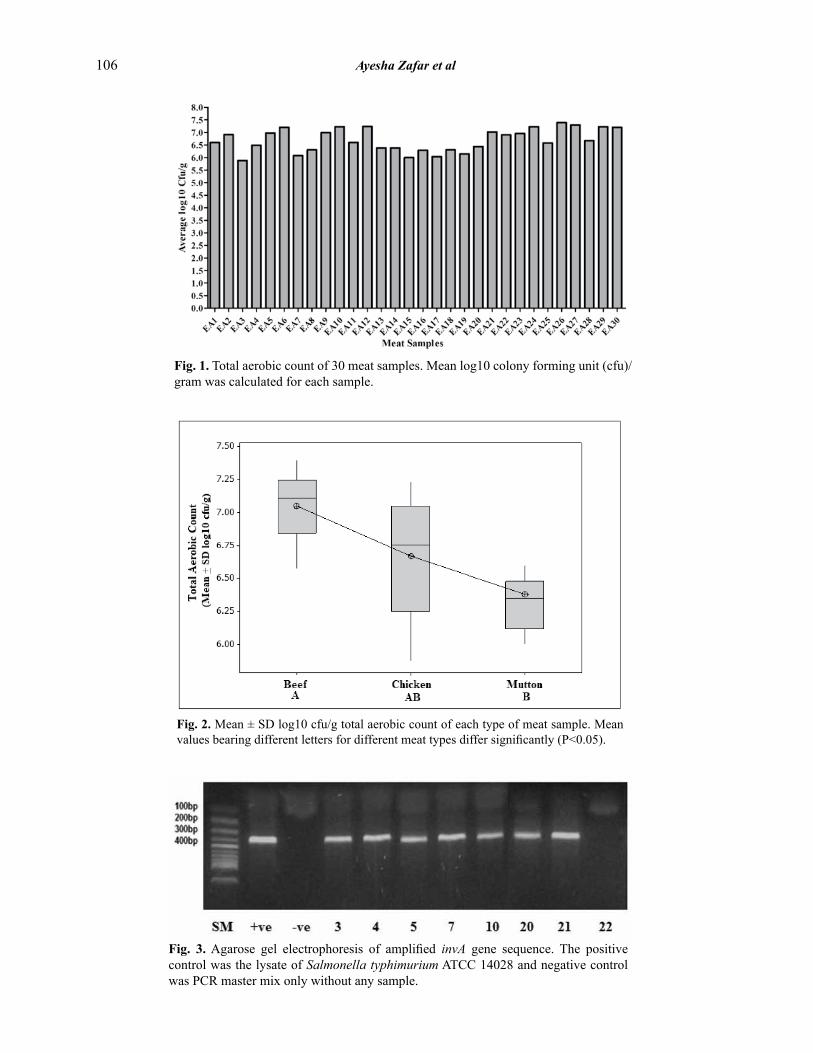
106 Ayesha Zafar et al
Fig. 2. Mean ± SD log10 cfu/g total aerobic count of each type of meat sample. Mean values bearing different letters for different meat types differ significantly (P<0.05).
Fig. 1. Total aerobic count of 30 meat samples. Mean log10 colony forming unit (cfu)/ gram was calculated for each sample.
Fig. 3. Agarose gel electrophoresis of amplified invA gene sequence. The positive control was the lysate of Salmonella typhimurium ATCC 14028 and negative control was PCR master mix only without any sample.

Microbial Evaluation of Raw Meat Products 107
amplify 389bp PCR product (Fig. 3). The primers and conditions described earlier were used to perform Salmonella PCR [8]. It was found that 13 out 30 tested samples were positive for Salmonella spp. (Table 1). Salmonella was more prevalent in chicken samples as 6 out of 10 samples were positive followed by 5 out of 10 in beef and only 2 positive samples of mutton (Fig. 4). It is apparent that the prevalence of Salmonella in chicken was higher as compared to mutton and beef and that the total percentage of positive meat samples among the 30 meat samples tested was found to be 43.33% which is a significant value to consider food hygiene. Raw meat samples which were positive for Salmonella in PCR were also confirmed by conventional detection methods and it was found that all the samples which were positive in PCR were also positive in cultural and biochemical identification (data not shown). The specific primers used in this study for PCR, were an amplified segment of around 389 base pairs present on InvA gene. This specific gene was selected due to the fact that it has been reported in all of the Salmonella serovars except some conflicting reports for S. pullorum and S. arizonae [14-16].
This study revealed that fresh meat products available in local markets are seriously contaminated with variety of microorganisms. The presence of higher number of organisms makes meat more
prone to spoilage and may serve as a tool for the transmission of pathogenic strains. The diseases of gastrointestinal tract are very common in this part of the world and they are mainly transmitted through contaminated food and water. It is largely due to improper handling, unhygienic conditions, lack of awareness and ignorance of regulatory authorities. Several studies in Pakistan have been conducted to see the microbiological quality of meat and meat products. In one such study 84% meat samples were found to be contaminated with variety of enteric organisms including some of the obligate pathogens [17]. Similar results were obtained in another study, when it was observed that chicken meat samples were heavily contaminated with coliforms and total bacterial count in Lahore, Pakistan [18].
4. CONCLUSIONS
In conclusion, high level of contamination was observed in all types of meat samples. Samples failed to meet any of the criteria made by different regulatory bodies of food and food products. The high level of contamination and presence of pathogens indicate the unhygienic handling of meat during slaughtering, processing and storing at retailers’ shop. These contaminated food items are routinely involved in several outbreaks of different infections and intoxications. So, it is a need of
Table 1. Total coliform count, fecal coliforms and Salmonella in meat samples.
Sample code
Sample MPN/g Fecal Coliforms
Salmonella Sample Code
Sample MPN/g Fecal Coliforms
Salmonella
EA 1 Chicken >1100 Positive Positive EA 16 Mutton >1100 Positive NegativeEA 2 Chicken <3 Negative Negative EA 17 Mutton >1100 Positive PositiveEA 3 Chicken >1100 Positive Positive EA 18 Mutton 1100 Positive NegativeEA 4 Chicken >1100 Positive Positive EA 19 Mutton 1100 Positive NegativeEA 5 Chicken >1100 Positive Positive EA 20 Mutton >1100 Positive PositiveEA 6 Chicken >1100 Positive Negative EA 21 Beef >1100 Negative PositiveEA 7 Chicken >1100 Positive Positive EA 22 Beef >1100 Negative NegativeEA 8 Chicken >1100 Positive Negative EA 23 Beef >1100 Positive NegativeEA 9 Chicken >1100 Positive Negative EA 24 Beef >1100 Positive Negative
EA 10 Chicken >1100 Positive Positive EA 25 Beef >1100 Positive NegativeEA 11 Mutton >1100 Positive Negative EA 26 Beef >1100 Positive PositiveEA 12 Mutton >1100 Negative Negative EA 27 Beef >1100 Positive PositiveEA 13 Mutton 1100 Positive Negative EA 28 Beef >1100 Positive PositiveEA 14 Mutton >1100 Positive Negative EA 29 Beef 150 Positive NegativeEA 15 Mutton 1100 Positive Negative EA 30 Beef >1100 Positive Positive
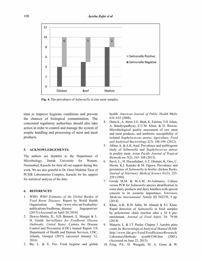
108 Ayesha Zafar et al
time to improve hygienic conditions and prevent the chances of biological contamination. The concerned regulatory authorities should also take action in order to control and manage the system of aseptic handling and processing of meat and meat products.
5. ACKNOWLEDGEMENTS:
The authors are thankful to the Department of Microbiology, Jinnah University for Women, Nazimabad, Karachi for their all out support during this work. We are also grateful to Dr. Omer Mukhtar Tarar of PCSIR Laboratories Complex, Karachi for his support for statistical analysis of the data.
6. REFERENCES
1. WHO. WHO Estimates of the Global Burden of Food Borne Diseases. Report by World Health Organization. http://www.who.int/foodsafety/publications/foodborne_disease/ fergreport/en/ (2015) (Accessed on April 20, 2016)
2. Dewey-Mattia, D., S.D. Bennett, E. Mungai & L. H. Gould. Surveillance for Foodborne Disease Outbreaks, United States. Centers for Disease Control and Prevention (CDC) Annual Report. US Department of Health and Human Services, CDC, Atlanta, Georgia (2015) (accessed January 12, 2016)
3. Bu, L. & E. Fee. Food hygiene and global
health. American Journal of Public Health 98(4): 634–635 (2008).
4. Datta S., A. Akter, I.G. Shah, K. Fatema, T.H. Islam, A. Bandyopadhyay, Z.U.M. Khan, & D. Biswas. Microbiological quality assessment of raw meat and meat products, and antibiotic susceptibility of isolated Staphylococcus aureus. Agriculture, Food and Analytical Bacteriology 2(3): 186-194. (2012).
5. Akbar, A. & A.K. Anal. Prevalence and antibiogram study of Salmonella and Staphylococcus aureus in poultry meat. Asian Pacific Journal of Tropical Biomedicine 3(2): 163–168 (2013).
6. Suvit, L., H. Hayashidani, A.T. Okatani, K. Ono, C. Hirota, K.I. Kaneko & M. Ogawa. Prevalence and persistence of Salmonella in broiler chicken flocks. Journal of Veterinary Medical Science 61(3): 255-259 (1999).
7. Gwida M.M. & M.A.M. Al-Ashmawy. Culture versus PCR for Salmonella species identification in some dairy products and dairy handlers with special concern to its zoonotic importance. Veterinary Medicine International. Article ID 502370, 5 pp. (2014).
8. Khan, A.B., K.H. Sahir, M. Ahmed & S.I. Khan. Rapid detection of Salmonella in food samples by polymerase chain reaction after a 10 h pre-enrichment. Journal of Food Safety 34: 79-86 (2014).
9. Maturin, L. & J.T. Peeler. Chapter 3. Aerobic plate count. In: Bacteriological Analytical Manual (BAM). http://www.fda.gov/Food/FoodScienceResearch/ LaboratoryMethods/ ucm063346.htm (2001). (Accessed on June 22, 2015).
10. Feng, P.S., D. Weagant, M. A. Grant & W.
Fig. 4. The prevalence of Salmonella in raw meat samples.

Microbial Evaluation of Raw Meat Products 109
Burkhardt. Chapter 4. Enumeration of Escherichia coli and the coliform bacteria. In: Bacteriological Analytical Manual (BAM). http://www.fda.gov/Food/FoodScienceResearch/LaboratoryMethods/ ucm064948.htm (2002). (Accessed on June 22, 2015).
11. Commission Regulation [EC] No. 2073/2005 of 15 November 2005 on microbiological criteria for food stuffs. In: Official Journal of the European Union. Published online by Food Safety Research Information Office, USDA, USA. https://www.fsai.ie/uploadedFiles/Reg2073_2005(1).pdf. (Accessed on May 7, 2016).
12. Chapter 13: Microbiological criteria. In: Meat Industry Guide. Published online by Food Standard Agency (UK). https://www.food.gov.uk/business-industry/meat/guidehygienemeat. (Accessed on May 07, 2016).
13. Microbiological criteria for foodstuffs-Part 1, GSO 1016/1998. GCC standardization organization, Riyadh, Kingdom of Saudi Arabia (1998).
14. Galan, J.E., C. Ginocchio & P. Costeas. Molecular and functional characterization of Salmonella
invasion gene InvA: Homology of InvA to members of a new protein family. Journal of Bacteriology 174: 4338-4349 (1992).
15. Moganedi, K.L.M., E.M.A. Goyvaerts, S.N. Venter & M.M. Sibara. Optimisation of the PCR-invA primers for the detection of Salmonella in drinking and surface waters following pre-cultivation step. Water SA 33: 196-202 (2007).
16. Radji, M., A. Malik & A. Widyasmara. Rapid detection of Salmonella in food and beverage samples by polymerase chain reaction. Malaysian Journal of Microbiology 6: 166-170 (2010).
17. Ali, N.H., A. Farooqui, A. Khan, A.Y. Khan & S.U. Kazmi. Microbial contamination of raw meat and its environment in retail shops in Karachi, Pakistan. The Journal of Infection in Developing Countries 4(6): 382-8 (2010).
18. Chaudhry, M., H. Rashid, M. Hussain, H.B. Rashid & M.D. Ahmad. Evaluation of bacteriological quality of whole chicken carcasses with and without skin by comparing level of indicator bacteria. Science International 23(4): 307-311 (2011).


Research Article
Proceedings of the Pakistan Academy of Sciences: Pakistan Academy of SciencesB. Life and Environmental Sciences 53 (2): 111–119 (2016)Copyright © Pakistan Academy of SciencesISSN: 0377 - 2969 (print), 2306 - 1448 (online)
————————————————Received, February 2016; Accepted, May 2016* Corresponding author: Alia Abbas; Email: [email protected]
New Fungal Records on Psidium guajava from Pakistan
Syed Qaiser Abbas1, Abida Perveen1, Sana Riaz1,Thereema Iftakhar1, and Alia Abbas2*
1Department of Botany, Government College University,Allama Iqbal Road, Faisalabad, Pakistan
2Department of Botany, Federal Urdu University, Karachi, Pakistan
Abstract: Aspergillus niger Van Tiegh, Chalara state of Ceratocystis fimbriata Ellis & Halst., Alternaria dianthicola Neergaard and Lasiodiplodia ricini Sacc. are reported for the first time on Psidium guajava from Faisalabad, Pakistan.
Keywords: Aspergillus niger, Chalara state of Ceratocystis fimbriata, Alternaria dianthicola, Lasiodiplodia ricini, Psidium guajava
1. INTRODUCTION
In a continuing project on survey and surveillance of fungal associations to the flora of district Faisalabad, Pakistan, a detailed survey of the area was carried out. The present article reports on the fungi observed on Psidium guajava L. (Guava; Amrud) belonging to family Myrtaceae. It is a small tree or shrub, about 6 meters tall. Flowers are white, Immature fruit ate green in color, while mature fruit varies in form, shape and colors. Its distribution and economic importance was fully discussed by [1]. Guava is grown worldwide and is reported to be stressed by a number of diseases including fungal diseases. Which are the most serious and devastating diseases, destroying thousands of trees annually, and it is also attaining the status of the national problem in Pakistan and India [2, 3, 4, 5, 6, 7, 8, 9, 10, 11]. Among the various diseases which attack guava plant, wilt is very destructive. This disease is caused by Fusarium solani, F. sp. Psidii, Fusarium oxysporum [3, 4, 5, 6]. This disease is characterized by yellowing and browning of leaves and tips of the twigs. Another important disease that is reported from Karachi and Faizabad (Rawalpindi) Pakistan is Anthracnose of guava caused by Gloeosporium
psidii that attack aerial parts of the plant resulting the death of branches [7, 11].
Twenty one (21) fungi have been reported from Pakistan [2, 3, 4, 5, 6, 7, 12, 13, 11]. Lodi et al. [14] have also reported. Pythium aphanedematum on Psidium guajava from Tando Fazal, District Hyderabad and Safari Park, Karachi. This is the first Oomycetous fungus, reported on Psidium guajava from Pakistan; thus, fungi reported on Psidium guajava from Pakistan become twenty two (22).
Recently, Abbas et al. [1] reported four (4) fungi from Faisalabad. Out of them 3 fungi viz., Rutola graminis (Desm.) Craneand Schokn.,Cladosporium nigrellum Ellis and Ever hand Gliomastix state of Wallrotheilla subiculosa were new records on it from Pakistan (Faisalabad). Alternaria tenuissima (Nees, ex Fr.) was previously reported from Pakistan, but not from Faisalabad, thus the total fungi recorded from Pakistan up to 2014 became twenty five (25).
In this article, four new fungi are reported from Faisalabad, Pakistan; thus the total number of fungi observed on Psidium guajava in Pakistan has been raised to twenty nine (29).

112 Syed Qaiser Abbas et al
2. MATERIALS AND METHODS
Samples of Psidium guajava were collected from the different areas of District Faisalabad and Jhang. Areas from District Faisalabad included GC University, Faisalabad, University of Agriculture, Faisalabad, Sheikh Colony Faisalabad and District Jhang include suburb area of Jhang city.
Materials and Methods used were the same as described by [15]. Identification up to species level were carried out after consulting [16, 2, 17, 18, 19, 20, 21].
3. RESULTS AND DISCUSSION
I) The fungus found on Psidium guajava specimen #.14, identified as Aspergillus niger Van Teigh., Annales des Sciences Naturelles; Botanique, 5,
8: 240 (1867) Fig. 1, (A & B).
Description of the Fungus
Mycelium immersed. Conidiophores erect, straight or flexuous, often up to 500 µm long, and 11-16 µm wide, hyaline or with the upper part brown, swollen at the apex into spherical vesicle which is usually 33-56 µm in diameter. Conidiogenous cells, hologenous stationary, flaskshaped. Conidia basipetal, catenate, dry, usually globose, brown, verruculose or echinulate, sometimes with the warts or spines arranged in discontinuous bands, 2.4-4.6 µm in diameter.
In the present studies the fungus identified as Aspergillus niger Van Teigh. This fungus is very common air contaminant and reported from all over the Pakistan. However it is not recorded on Psidium
Table 1. Total species of Lasiodiplodia spp. with reference to conidial measurement.
Name of species Conidialmeasurement(μm) Reference L. abnormis 25–28 × 13–15 [39]L. citricola 22.5–26.6 × 13.6–17.2 [16] L. crassispora 27–30 × 14–17 [34] L. fiorii 24–26 × 12–15 [23]L .gilanensis 28.6 – 33.4 × 15.6 – 17.6 [16]
L. gonubiensis 32–36 × 16–18.5 [36]
L. hormozganensis 19.6–23.4 × 11.7–13.3 [16]L. iraniensis 18.7–22.7 × 12.1–13.9 [16]L. margaritacea 14–17 × 11–12 [36]L. paraphysaria 30–32 × 15–16 [39] The fungus investigated in this study 16-18× 10-11 This publicationL. parva 18.3–22.1 × 10.7–12.3 Alves et al. (20 [33] L. plurivora 26.7–32.5 × 14.4–16.7 [35]L. pseudotheobromae 25.5–30.5 × 14.8–17.2 [33]
21.7–26.3 13.4–14.8 Abdollahzade [16] L. ricini 16–19 × 10–11 [39] L. rubropurpurea 24–33 × 13–17 [34] L. theobromae 25.5–30.5 × 14.8–17.2 [33] L. theobromae 22.4–24.2 × 12.9–14.3 [16] L. thomasiana 28–30 × 11–12 [39] L. undulata 20–32 × 13.5–19.2 [26]
L. venezuelensis 26–33 × 12–15 [34]
Abdollahzadehet al.[16]
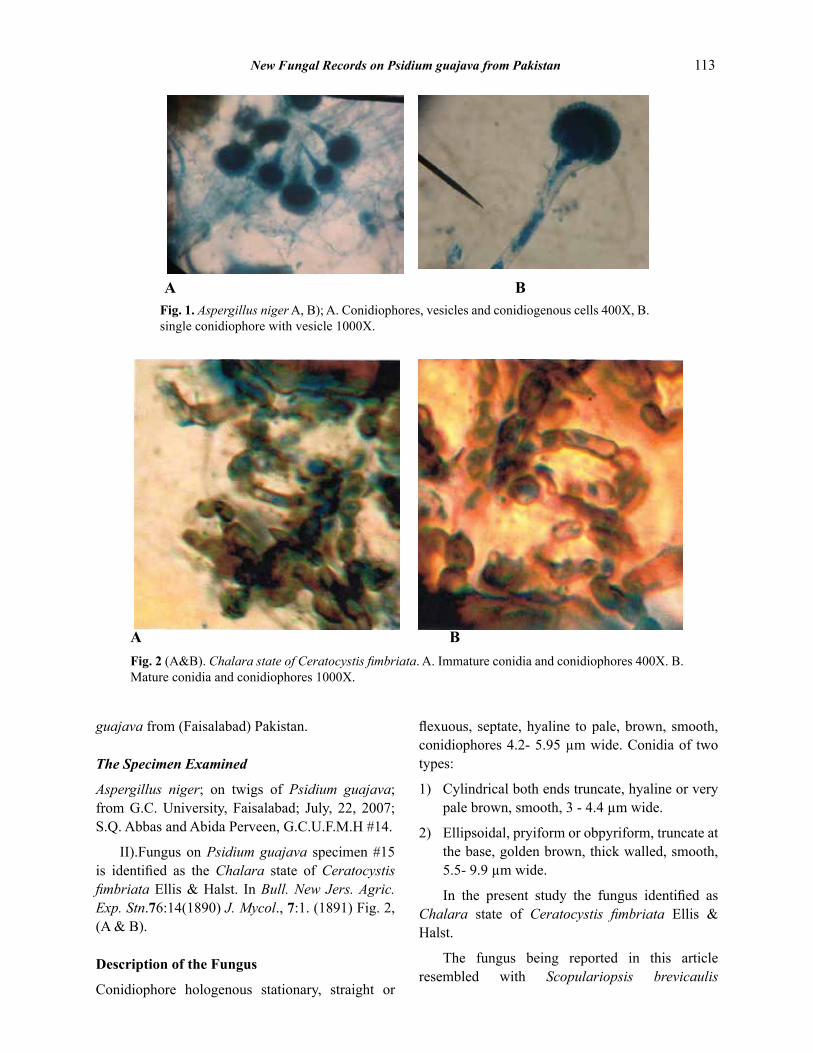
New Fungal Records on Psidium guajava from Pakistan 113
guajava from (Faisalabad) Pakistan.
The Specimen Examined
Aspergillus niger; on twigs of Psidium guajava; from G.C. University, Faisalabad; July, 22, 2007; S.Q. Abbas and Abida Perveen, G.C.U.F.M.H #14.
II).Fungus on Psidium guajava specimen #15 is identified as the Chalara state of Ceratocystis fimbriata Ellis & Halst. In Bull. New Jers. Agric. Exp. Stn.76:14(1890) J. Mycol., 7:1. (1891) Fig. 2, (A & B).
Description of the Fungus
Conidiophore hologenous stationary, straight or
flexuous, septate, hyaline to pale, brown, smooth, conidiophores 4.2- 5.95 µm wide. Conidia of two types:
1) Cylindrical both ends truncate, hyaline or very pale brown, smooth, 3 - 4.4 µm wide.
2) Ellipsoidal, pryiform or obpyriform, truncate at the base, golden brown, thick walled, smooth, 5.5- 9.9 µm wide.
In the present study the fungus identified as Chalara state of Ceratocystis fimbriata Ellis & Halst.
The fungus being reported in this article resembled with Scopulariopsis brevicaulis
Fig. 1. Aspergillus niger A, B); A. Conidiophores, vesicles and conidiogenous cells 400X, B. single conidiophore with vesicle 1000X.
Fig. 2 (A&B). Chalara state of Ceratocystis fimbriata. A. Immature conidia and conidiophores 400X. B. Mature conidia and conidiophores 1000X.
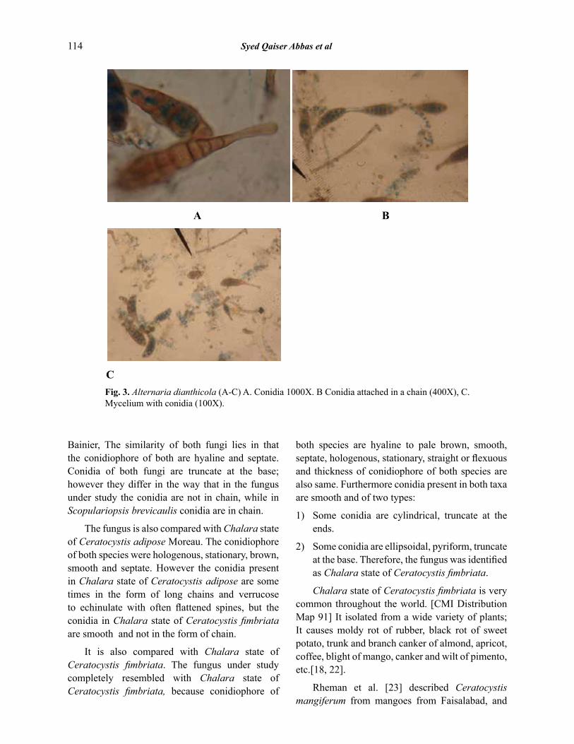
114 Syed Qaiser Abbas et al
Fig. 3. Alternaria dianthicola (A-C) A. Conidia 1000X. B Conidia attached in a chain (400X), C. Mycelium with conidia (100X).
Bainier, The similarity of both fungi lies in that the conidiophore of both are hyaline and septate. Conidia of both fungi are truncate at the base; however they differ in the way that in the fungus under study the conidia are not in chain, while in Scopulariopsis brevicaulis conidia are in chain.
The fungus is also compared with Chalara state of Ceratocystis adipose Moreau. The conidiophore of both species were hologenous, stationary, brown, smooth and septate. However the conidia present in Chalara state of Ceratocystis adipose are some times in the form of long chains and verrucose to echinulate with often flattened spines, but the conidia in Chalara state of Ceratocystis fimbriata are smooth and not in the form of chain.
It is also compared with Chalara state of Ceratocystis fimbriata. The fungus under study completely resembled with Chalara state of Ceratocystis fimbriata, because conidiophore of
both species are hyaline to pale brown, smooth, septate, hologenous, stationary, straight or flexuous and thickness of conidiophore of both species are also same. Furthermore conidia present in both taxa are smooth and of two types:
1) Some conidia are cylindrical, truncate at the ends.
2) Some conidia are ellipsoidal, pyriform, truncate at the base. Therefore, the fungus was identified as Chalara state of Ceratocystis fimbriata.
Chalara state of Ceratocystis fimbriata is very common throughout the world. [CMI Distribution Map 91] It isolated from a wide variety of plants; It causes moldy rot of rubber, black rot of sweet potato, trunk and branch canker of almond, apricot, coffee, blight of mango, canker and wilt of pimento, etc.[18, 22].
Rheman et al. [23] described Ceratocystis mangiferum from mangoes from Faisalabad, and

New Fungal Records on Psidium guajava from Pakistan 115
Fig. 4(A-C). Lasiodiplodia ricini. A. Immature conidia and conidiogenous cells 400x, B. Mature conidia 400x. C. Mature conidia 1000.
the fungus on Psidium guajavais also reported from Faisalabad, therefore acritical study of the type of Ceratocystis mangiferum is necessary. Previously, there was no record of this fungus found from Pakistan[2]. In the present study, the fungus under study is a new report for Pakistan. Moreover Psidium guajava is also a new host for this fungus, from Pakistan.
The Specimen Examined
Chalara state of Ceratocystis fimbriata; on bark of Psidium guajva; Jhang Road, Faisalabad; August 24, 2007; S.Q. Abbas and AbidaPerveen, G.C.U.F.M.H.# 15.
III).A fungus found on Psidium guajava G.C.U.F.M.H # 17, identified as Alternaria dianthicola Neergaard, Neergaard, Danish species of Alternaria and Stemphylium: 190 (1945). Fig. 3, (A-C).
Description of the Fungus
Conidiophores pale olivaceous brown, septate, arising singly or in branched, straight or flexuous. The conidiophore 151 x 3.84-6.52 µm. Conidia straight or curved, obclavate or almost cylindrical, rostrate, pale olivaceous brown, smooth, with 4-12 transverse and up to 3 longitudinal or oblique septa, constricted at the septa, 56-136 x 10.5- 17.5 µm. The colour of beak and conidial body is same, sometimes inflated at the tip.
The fungus is identified as Alternaria dianthicola is compared with related species of Alternaria.
Alternaria ricini Hansford, resembles with the fungus under study. Colonies of both species are brown and conidiophore of both taxa arising singly or in groups, erect, simple, straight or flexuous. However they differ from each other in conidiophores measurement. Conidiophores of
116 Syed Qaiser Abbas et al
Alternaria ricini are 80 x 5-9 µm, and 150 x 4-6 µm in fungus under study. Number of transverse septa in conidia of Alternaria ricini are 5-10 and4-12 µm in the fungus under study. Fungus under study also differs from A. solani and A. longipes, because conidia in A. solani are 150-300 x 15-19 µm and in A. longipes conidia are 35-110(69) x 11-21(14) µm, whereas in fungus under study the conidia are of 56-136 x 10.5- 17.5 µm and smaller than A. solani and A. longipes.
Alternaria pedwickii Ellis., resemble closely with the fungus under study in shape of conidia, however both differ due to the size of conidiophores i.e. 180 x 3-4 µm in the Alternaria pedwickii and 151 x 3.84-6.52 µm in the fungus under study. Similarly they also differ in conidial measurement. Conidia in Alternaria pedwickii are 95-170 x 11-20 µm and 56- 136 x 10.5- 17.5 µm in the fungus under study.
Alternaria cucumerina also differs from fungus under study as conidia are more longer and wider in Alternaria cucumerina 130-220 (180) x 15-24 (20)µm, than in the fungus under study 56- 136 x 10.5- 17.5 µm. Similarly conidiophores in Alternaria cucumerina are wider i.e. of 110 x 6-10 µm than the fungus under study 3.84- 6.52 µm. Alternaria sonchi Davis, can also be differentiated from fungus under study. Conidia in Alternariasonchi are smaller but wider, 60- 130(77) x 15-26 µm and conidia are longer and less wider5 6- 136 x 10.5- 17.5 µm in the fungus under study, Similarly, conidiophores of Alternaria sonchi are smaller but wider 80 x 5-9 µm than the fungus under study 151 x 3.84- 6.52 µm.
The fungus completely resembles with Alternaria dianthicola, because the fungus under study shares all the characteristics with Alternaria dianthicola. The conidiophores measurement in Alternaria dianthicola are 150 x 4-6 µm and in the fungus under study are 151 x 3.84- 6.52 µm. Furthermore in both taxa conidiophore are brown, similarly conidial measurement also coincide with each other, conidia in Alternaria dianthicola are 55-130 (93) x 10-16 (13) µm thick in the broadest part and 56- 136 x 10.5- 17.5 µm in the fungus under study. Therefore it is identified as Alternaria dianthicola.
Twenty nine species of genus Alternaria are already reported from Pakistan [2]. This fungus was reported from Australia, Chile, Denmark, France, Germany, Italy, Jamaica, Malawi, Malaya, Netherlands, New Zealand, U.S.A. [18, 19].However it is not reported from Pakistan [2].
In the present study Alternaria dianthicola observed for the first time on Psidium guajava from (Faisalabad), Pakistan.
The Specimen Examined
Alternaria dianthicola on leaves of Psidium guajava, GC University, Faisalabad; 5 August, 2007; S.Q. Abbas and Abida Perveen, G.C.U.F.M.H# 17.
Fungus on Psidium guajava specimen No. G.C.U.M.H No. 21 is identified as Lasiodiplodia ricini Sacc. Nuovo G. bot. ital. 22(1): 61 (1915). Fig. 4, A-C.
Description of the Fungus
Mycelium immersed, conidiomatastromatic. Ostiole absent. Conidiophore absent. Conidiogenous cells hologenous, no proliferation, hyaline. Immature conidia hyaline and thin walled. Mature conidia brown, oval both ends obtuse, uniseptate, euseptate and present in the middle of the conidia. Thick walled with many longitudinal striations.
Sutton [24]was of the opinion that Lasiodiplodia theobromae is the correct name of Botrydiplodia theobromae. However, Punithalingum (1980) [25] retained it as Botryodiplodia theobromae in his monograph.
Abbas et al.[26] when they were assessing the Sphaeropsis undulata Berk. &Curt., they pointed out that Sphaeropsis undulata is an earlier name for Lasiodiplodia theobromae (as Botryodiplodia theobromae), therefore a new combination Lasiodiplodia undulata (Berk. & Curt.) Abbas, Sutton, Ghaffar & Abbas was proposed.
Lasiodiplodia undulata (as Botryodiplodia theobromae) was reported on 41 plants belonging to different families from Pakistan, This fungus cause diseases on Albizia lebbeck, Aloevera (as Aloe barbadensis), Althurium andraeanum, Arachis hypogaea, Argyreia speciosa, Bauhinia veriegata, Bignonia sp., Broussonetia papyrifera,

New Fungal Records on Psidium guajava from Pakistan 117
Borassus flabellifer, Cappris decidua as Cappris aphylla), Citrus auratium, Citrus aurantifolia, Cosmos sulphureus, Dalbergia sissoo, Erythrina indica, Euphorbia tirucalli, Ficus palmata, Ficus retusa, Gossypium neglectum, Gossypium sp. Helianthus annus, Ipomoea carnea. Ipomoea gossypiodes, Lagenaria siciraria (as Lagenaria vulgaris), Mangifera indica, Mimosa subicaulis, Maniho tesculenta (as Manihot utilissima), Melia azedarach, Moringa oleifera, Morus alba, Nerium oleander (as Nerium indicum), Pandanus tectorius (as Pandanus odaratissimus), Pedilanthus tithymaloides, Prosopis julifora, Prosopis spicigera, Psidium guajava, Withania somnifera, Catharanthus roseus (as Vincarosea), Znniasp, Ziziphus mauritiana on dead branches of from Lahore, Changa Manga, Ladhar (Sheikhupura); Faisalabad, Tondo Jam, Bimber, Karachi [15, 27, 28, 29, 30, 2, 6, 31, 32, 13].
In recent years morphological as well on DNA finger printing and sequence work was carried out (9, 16, 33, 34, 35, 36.]. Abdollahzadeh et al. [16] carried out a detail studies on Lasiodiplodia theobromae described from different part of world using morphological as well on DNA finger printing and sequenceand accepted 14 species of Lasiodiplodia. Abdollahzadeh et al [16] were of the opinion that conidial dimension of Botryodiplodia theobromae never exceed 30 µm. in length and 16 µm. in width, while the conidial length in Lasiodiplodia undulata are up to 32 µm. and width is up to 19.2 µm. Therefore they consider that both species are separate taxa. Fungus under study is identified as Lasiodiplodia ricini Sacc., due to conidial and pycnidial morphology and dimensional characters.
Lasiodiplodia ricini Sacc. can easily can be differentiated by Botryodiplodia ricinicola (Sacc.)Petr.[37], which has bigger and wider conidia (22-30 x 12-16 µm). Botryodiplodia ricinincola Ahmad, Nom. rej. [38] also differs from Lasiodiplodia ricini Sacc. in having bigger and slightly wider conidia 17-28 X 11-12 µm.
Botryodiplodia theobromae was also reported on Psidium guajava from Tando Jam Sindh, Pakistan Khan and Kamal (1968) [8]. However it is not reported from Faisalabad, Punjab, Pakistan [2].
The fungus under study (conidia 16-18× 10-11 µm) differs from the following Lasiodiplodia spp. In having bigger conidia viz.;- L. abnormis (25 - 28 × 13 - 15 µm); L. citricola (22.5 - 26.6 × 13.6 - 17.2 µm); L. crassispora (27 - 30 × 14 - 17 µm); L. fioriii (24 - 26 × 12 - 15 µm); L. hormozganensis (19.6 - 23.4 × 11.7 - 13.3 µm); L. iraniensis (18.7 - 22.7 × 12.1- 13.9 µm); L. parva (18.3 - 22.1 × 10.7 - 12.3 µm); L. pseudotheobromae [; (25.5 - 30.5× 14.8 - 17.2 µm [33]; (21.7 - 26.3 × 13.4 - 14.8 µm;) [16]; L. theobromae [(23.6–28.8 × 13–15.4 µm) [33];`(22.4 - 24.2 × 12.9 - 14.3 µm) [16]; L. gonubiensis (32 - 36 × 1 6 - 18.5 µm ) ; L. gilanensis (28.6 - 33.4 × 15.6 - 17.6 µm ); L. thomasiana (28 - 30 × 11 - 12 µm) and L. undulata (20 - 32 × 13.5 - 19.2 µm); L. venezuelensis (26–33 × 12–15 µm). It differs from L. margaritacea (14 - 17 × 11 - 12 µm) which has smaller conidia. Fungus under study completely resembles with L. ricini (16–19 × 10–11) in conidial morphology and dimensions. In the present studies, Lasiodiplodia ricini is a new report on Psidium guajava from Pakistan (Faisalabad).
Work of Abdollahzadeh et al. (2010) [16] is very important therefore, it is necessary that all the fungi described as Lasiodiplodia undulata (Lasiodiplodia theobromae, or Botryodiplodia theobromae) on different hosts from Pakistan needs an urgent revision in the light of morphological and DNA finger printing and sequence.
Specimen Examined
Lasiodiplodia ricini identified from the bark of Psidium guajava; Jhang Road garden; October 2, 2007: S.Q. Abbas and Abida Perveen, G.C.U.M.H # 21.
4. REFERENCES
1. Abbas, S.Q., A. Perveen, M. Naiz, S. Riaz, T. Iftikhar & A. Abbas. New fungal records on Psidium guajava from Pakistan. Proceeding of the Pakistan Academy of Science 15 (2): 121-127 (2014).
2. Ahmad, S., S.H. Iqbal & A.N. Khalid. Fungi of Pakistan. Sultan Ahmad. Mycological Society of Pakistan, Department of Botany, University of the Punjab, Lahore, Pakistan (1997).
3. Bhatti, A.G., N.J. Ismail, A.M. Lodhi & W.A. Maitlo. Isolation and identification of fungi causing detritions of guava (Psidium guajava L.) in Larkana, Sindh. In: Abstracts “Challenges and

118 Syed Qaiser Abbas et al
Options for Plant Health Management”, 8th National Conf. of Pakistan Phytopathological Society 28-29 November, 2011, University of Agriculture, Faisalabad, Pakistan, p. 64 (2011).
4. Bokhari, A.A. & S.T. Sahi. Studies on Guava decline and disease management in Pakistan. In: Abstracts “Challenges and Options for Plant Health Management”, 8th National conf. of Pakistan Phytopathological Society, 28-29 November, 2011, University of Agriculture, Faisalabad, Pakistan, p. 64 (2011).
5. Fateh, F. S., M. R. Kazmi, I. Ahmad & T. Mukhtar. Common fungi found in decline affected Mango and Gauva orchids in Punjab. In: Abstracts 8th
National conference of Pakistan Phytopathological Society. Challenges and options for plant health management” Nov. 28-29, 2011, p. 30. Faisalabad Pakistan (2011).
6. Ghaffar, A. & A. Kafi. Fungi of Karachi. Pakistan Journal of Botany 4: 195-208 (1968).
7. Ghafoor, A. & S.A.J. Khan. List of Diseases of Economic Plants in Pakistan. Department of Plant Protection, Ministry of Food, Agriculture and Under Developed Areas, Government of Pakistan, 85 pp. (1976).
8. Khan, S. A. & M. Kamal. Additions to the parasitic fungi of Pakistan. I. Mycopathologiaet Mycolologia. Applicata 39: 193-208 (1969).
9. Palvic, D., M. J. Wingfield, P. Baber, B. Slippers, G. E.S. Hardy & T.I. Burgess. Seven new species of Botryspaertaceae from baobob and other natives trees in Western Australia. Mycologia 100: 851-866 (2008).
10. Singh, S.J. Diseases of Fruit Crops in India, 1sted. Kalyani Publisher, New Dehli, India (1996).
11. Shakir, A.S., M. A. Nasir & S.T. Sahi. Anthracnose of Guajava (Psidium guajava) a new record in Pakistan. Pakistan Journal of Agricultural Science 28: 211 (1991).
12. Kafi, A. & Z.A. Siddique. Russetting of guavas in Karachi-Malir area Abs. Pak. Sci. Conf. A: 56 (1964).
13. Khan, A.H. Pathology of Trees. University of Agriculture, Faisalabad. Vol. II: p. 379-382. 201(1989).
14. Lodi, A.M., M.A., Khanzada, S. Shazad & A. Ghaffar .Prevalence of Pythium aphanidermatum in agro-ecosystem of Sindh province of Pakistan. Pakistan Journal Botany 45 (2): 635-642 (2013).
15. Abbas, S.Q., M. Naiz, R. Ayesha, T. Iftikhar & I. Ali. New fungal records on Morus alba from Faisalabad Pakistan. Pakistan Journal Botany 42:583-592 (2010).
16. Abdollahzadeh, J., A. Javadi, E. Mohammadi, Goltapeh, R. Zare, & A.J.L Phillips. Phylogeny and Morphology of four new species of Lasiodiplodia
from Iran. Persoonia. 25:1-10 (2010).17. Carmichael, J.W., W.B. Kendrick, I. L. Conners &
L. Sigler. Genera of Hyphomycetes. The University of Alberta Press. pp. 386 (1980).
18. Ellis, M.B. Dematiaceous Hyphomycetes. CAB (MI) Kew, Surrey, England, pp. 608 (1971).
19. Ellis, M.B. More Dematiaceous Hyphomycetes.CAB (MI) Kew, Pp. 507. (1976).
20. Kirk, P.M., Index fungorum data base CAB. UK. (2016)
21. Snowdon, A.L. A Colour Atlas of Postharvest Diseases and Disorders of Fruits and Vegetables. Vol. 1. General Introduction and Fruits. Wilfe Scientific Baralona, Spain. (1990).
22. Nag Raj, T.R. & B. Kendrick. A monograph of Chalara and allied genera. Department of Biology University Waterloo. Waterllo, Onterio, Canada. pp. 200 (1975).
23. Rheman, A., R. Anjum, I.A. Khan, A.S. Khan & I. Ahmad. Morphological characterization of Ceratocysti smangiferum sp. nov. isolate cause of Mango sudden death syndrome from Pakistan Challenges and options for plant health management Abstracts “8th National conf. of Pakistan Phytopathological Society” Nov. 28-29, 2011. p. 41 Faisalabad, Pakistan (2011).
24. Sutton, B.C. The Coelomycetes (CAB, IMI), Kew, Surrey, U.K. 696 pp. (1980).
25. Petrk, F. & S. Ahmad (1954). Bietragezurpilzflora Pakistan Sydowia 8 (1-6): 162-184 (1929).
26. Abbas, S.Q., B.C. Sutton, A. Ghaffar & A. Abbas. Reassessment of Sphaeropsis undulata Berk. & Curt. Pakistan Journal of Botany 36 (1) 209-218 (2004)
27. Ahmad, S. Further contributions to the fungi of Pakistan. 11. Biologia, 8: 123- 150 (1962).
28. Ahmad, S. Contributions to the fungi of Pakistan. VII. Biologia 14: 1-11 (1968).
29. Ahmad, S. Contributions to the fungi of Pakistan. XIII. Biologia, 18: 1- 16 (1972).
30. Ahmad, S. & M. Arshad. Contributions to the fungi of West Pakistan. XIII. Biologia 18: 7-17(1972).
31. Ghaffar, A., S.Q. Abbas & A. Kafi. Fungi of Karachi.Suppl. I. Pakistan Journal of Botany, 123: 261-266 (1971).
32. Ghaffar, A. and S.Q. Abbas. Fungi of Karachi: Suppl. II, Pakistan Journal of Botany, 4: 195-208 (1972).
33. Alves, A., P. W. Crous, A. Correia & A.J.L. Phillips. Morphological and Molecular data reveal cryptic species in Lasiodiplodia theobromae. Fungal Diversity, 28: 1-13 (2008).
34. Burgress T.I., P. A. Barbera, S. Mohali, G. Pegg, W. de., Beer & M.J. Wingfield. Three new Lasiodiplodia spp., from tropics recognized on DNA sequence comparisons and morphology. Mycologia, 98: 423-

New Fungal Records on Psidium guajava from Pakistan 119
435 (2006).35. Damma, U., P.W. Crous & P.H. Fourie.
Botryshaeriaceae as potential pathogens of Prunus in South Africa, with description of Diplodiaricana and Lasiodiplodia plurivora sp. nov. Mycologia 99: 664-680 (2007).
36. Palvic, D., B. Slippers, T.A. Coutinhu, M. Gryzenhout & M.J. Wingfield. Lasiodiplodiagombiensis sp.
nov. a new Botrysphaeria sanamorph from native Syzygium cordatum South Africa. Studies in Mycology 50: 313-322 (2004).
37. Pathak, V. N. Disease of Fruits Crops, 2nd ed. Oxford & IBH Pub. Co. New Delhi, 309 pp. (1986).
38. Ahmad, S., Fungi of Pakistan. Sydowia 2:72-78. (1948)
39. Saccardo, P. SylI. Sacc. Fungorum 22:1012 (1913).


Research Article
Proceedings of the Pakistan Academy of Sciences: Pakistan Academy of SciencesB. Life and Environmental Sciences 53 (2): 121–128 (2016)Copyright © Pakistan Academy of SciencesISSN: 0377 - 2969 (print), 2306 - 1448 (online)
Wakeby Distribution Modelling of Rainfall and Thunderstorm over Northern Areas of Pakistan
Naeem Sadiq*
Institute of Space and Planetary Astrophysics,
University of Karachi, Karachi 75270, Pakistan
Abstract: Five parametric Wakeby (L-moment) distribution has been compared with Gaussian, Gumbell and Generalized Extreme Value (GEV) for representing the rainfall and thunderstorm activities over four stations in the Northern areas of Pakistan (viz., Astore, Bunji, Garhi Dupatta and Muzaffarabad) for the period of 1961-2010. The test statistics of Kolmogorov-Smirnov test based on the empirical cumulative distribution function revealed that Wakeby modelling is quite suitable to model rainfall frequencies over all the considered stations while the same distribution also shows better model fittings for Astore, Garhi Dupatta and Muzaffarabad with exceptional case of Bunji where Gumbell distribution has a slightly better fit than the Wakeby. The intent of this paper is to present a contemporary statistical view of rainfall and thunderstorm investigation for the considered stations. Keywords: Wakeby distribution, Gaussian distribution, Probabilistic modelling
1. INTRODUCTION Thunderstorm (TS) and Rainfall (RF) events can cause severe damage to infrastructure in addition to tragic loss of lives [1]. However, predicting frequency of these parameters within a geographical area is an information problem. With the help of sufficiently long meteorological records, the distribution of frequency for a site may be estimated with a certain degree of accurately. In general, these distributions of the doubtful phenomena aren’t apprehended with certainty. If they were known, even then their functional representation would likely have too many parameters to be of much applied usage [2]. The pragmatic issue is the selection of a simple, suitable and reasonable distribution to get a description of the phenomenon under consideration, and then estimate the parameters of that distribution which finally leads to risk estimates with reasonable and acceptable accuracy for the considered problem [3]. The modelling of hydro-meteorological
related structures in weather modifications and climate changes monitoring is important and essential [4]. In this relation, rainfall and thunderstorm activities usually in monsoon season has been of great importance. In principle, climatologists have to fit different distributions to hydro-meteorological data to estimate a number return levels of extreme rainfalls [5]. Five parametric Wakeby (W5) distribution can copycat the outlines of a lot of more often than not used skewed distributions, as it comprises of five parameters. Because of its flexible nature it may prove to be sufficiently good fit to observed meteorological data parameter like rainfall etc. Many researchers used this distribution for other frequential analyses regarding different purposes [6-13] and they found this distribution to be more appropriate for the modelling of low flow discharges during flood frequency analyses. From this place, W5 is used to a great degree in hydro-meteorological applications in a successful manner, especially for the modelling
————————————————Received, September 2015; Accepted, May 2016Email: [email protected]
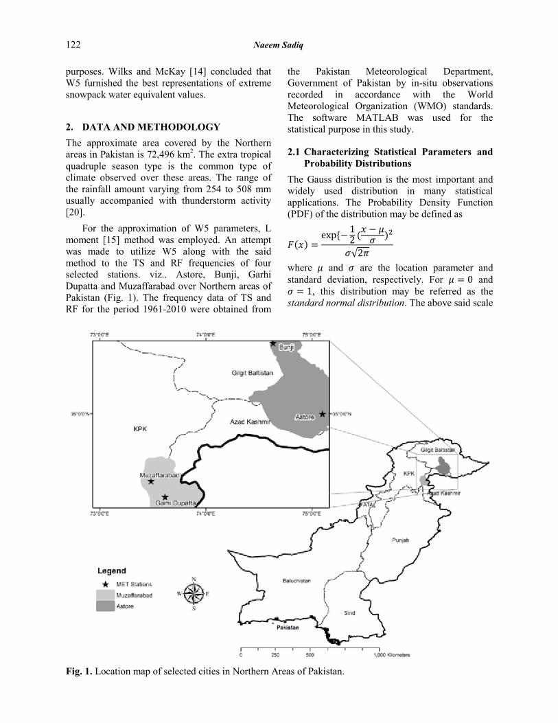
purposes. Wilks and McKay [14] concluded that W5 furnished the best representations of extreme snowpack water equivalent values. 2. DATA AND METHODOLOGY The approximate area covered by the Northern areas in Pakistan is 72,496 km2. The extra tropical quadruple season type is the common type of climate observed over these areas. The range of the rainfall amount varying from 254 to 508 mm usually accompanied with thunderstorm activity [20]. For the approximation of W5 parameters, L moment [15] method was employed. An attempt was made to utilize W5 along with the said method to the TS and RF frequencies of four selected stations. viz.. Astore, Bunji, Garhi Dupatta and Muzaffarabad over Northern areas of Pakistan (Fig. 1). The frequency data of TS and RF for the period 1961-2010 were obtained from
the Pakistan Meteorological Department, Government of Pakistan by in-situ observations recorded in accordance with the World Meteorological Organization (WMO) standards. The software MATLAB was used for the statistical purpose in this study.
2.1 Characterizing Statistical Parameters and Probability Distributions
The Gauss distribution is the most important and widely used distribution in many statistical applications. The Probability Density Function (PDF) of the distribution may be defined as
𝐹𝐹(𝑥𝑥) =exp {−1
2 (𝑥𝑥 − 𝜇𝜇𝜎𝜎 )2
𝜎𝜎√2𝜋𝜋
where 𝜇𝜇 and 𝜎𝜎 are the location parameter and standard deviation, respectively. For 𝜇𝜇 = 0 and 𝜎𝜎 = 1, this distribution may be referred as the standard normal distribution. The above said scale
Fig. 1. Location map of selected cities in Northern Areas of Pakistan.
122 Naeem Sadiq
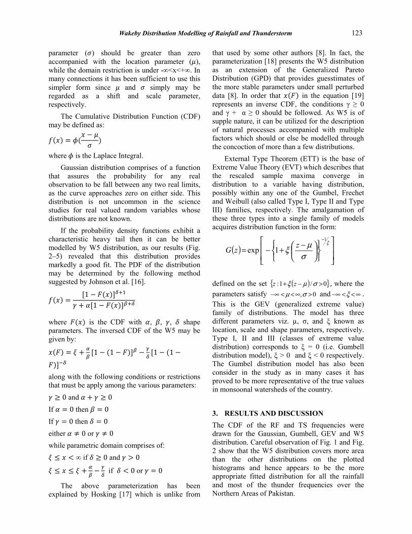
parameter (𝜎𝜎) should be greater than zero accompanied with the location parameter (𝜇𝜇), while the domain restriction is under -∞<x<+∞. In many connections it has been sufficient to use this simpler form since 𝜇𝜇 and 𝜎𝜎 simply may be regarded as a shift and scale parameter, respectively. The Cumulative Distribution Function (CDF) may be defined as:
𝑓𝑓(𝑥𝑥) = 𝜙𝜙(𝑥𝑥 − 𝜇𝜇𝜎𝜎
)
where 𝜙𝜙 is the Laplace Integral. Gaussian distribution comprises of a function that assures the probability for any real observation to be fall between any two real limits, as the curve approaches zero on either side. This distribution is not uncommon in the science studies for real valued random variables whose distributions are not known. If the probability density functions exhibit a characteristic heavy tail then it can be better modelled by W5 distribution, as our results (Fig. 2–5) revealed that this distribution provides markedly a good fit. The PDF of the distribution may be determined by the following method suggested by Johnson et al. [16].
𝑓𝑓(𝑥𝑥) =[1 − 𝐹𝐹(𝑥𝑥)]𝛿𝛿+1
𝛾𝛾 + 𝛼𝛼[1 − 𝐹𝐹(𝑥𝑥)]𝛽𝛽+𝛿𝛿
where 𝐹𝐹(𝑥𝑥) is the CDF with 𝛼𝛼, 𝛽𝛽, 𝛾𝛾, 𝛿𝛿 shape parameters. The inversed CDF of the W5 may be given by:
𝑥𝑥(𝐹𝐹) = 𝜉𝜉 + 𝛼𝛼𝛽𝛽
[1 − (1 − 𝐹𝐹)]𝛽𝛽 − 𝛾𝛾𝛿𝛿
[1 − (1 −
𝐹𝐹)]−𝛿𝛿 along with the following conditions or restrictions that must be apply among the various parameters: 𝛾𝛾 ≥ 0 and 𝛼𝛼 + 𝛾𝛾 ≥ 0 If 𝛼𝛼 = 0 then 𝛽𝛽 = 0 If 𝛾𝛾 = 0 then 𝛿𝛿 = 0 either 𝛼𝛼 ≠ 0 or 𝛾𝛾 ≠ 0 while parametric domain comprises of: 𝜉𝜉 ≤ 𝑥𝑥 < ∞ if 𝛿𝛿 ≥ 0 and 𝛾𝛾 > 0
𝜉𝜉 ≤ 𝑥𝑥 ≤ 𝜉𝜉 + 𝛼𝛼𝛽𝛽− 𝛾𝛾
𝛿𝛿 if 𝛿𝛿 < 0 or 𝛾𝛾 = 0
The above parameterization has been explained by Hosking [17] which is unlike from
that used by some other authors [8]. In fact, the parameterization [18] presents the W5 distribution as an extension of the Generalized Pareto Distribution (GPD) that provides guesstimates of the more stable parameters under small perturbed data [8]. In order that 𝑥𝑥(𝐹𝐹) in the equation [19] represents an inverse CDF, the conditions γ ≥ 0 and γ + α ≥ 0 should be followed. As W5 is of supple nature, it can be utilized for the description of natural processes accompanied with multiple factors which should or else be modelled through the concoction of more than a few distributions. External Type Theorem (ETT) is the base of Extreme Value Theory (EVT) which describes that the rescaled sample maxima converge in distribution to a variable having distribution, possibly within any one of the Gumbel, Frechet and Weibull (also called Type I, Type II and Type III) families, respectively. The amalgamation of these three types into a single family of models acquires distribution function in the form:
( )
−+−=
−ξ
σµξ
1
1exp zzG
defined on the set ( ){ }0/1: >−+ σµξ zz , where the parameters satisfy 0, >∞<<−∞ σµ and ∞<<−∞ ξ . This is the GEV (generalized extreme value) family of distributions. The model has three different parameters viz. µ, σ, and ξ known as location, scale and shape parameters, respectively. Type I, II and III (classes of extreme value distribution) corresponds to ξ = 0 (i.e. Gumbell distribution model), ξ > 0 and ξ < 0 respectively. The Gumbel distribution model has also been consider in the study as in many cases it has proved to be more representative of the true values in monsoonal watersheds of the country. 3. RESULTS AND DISCUSSION The CDF of the RF and TS frequencies were drawn for the Gaussian, Gumbell, GEV and W5 distribution. Careful observation of Fig. 1 and Fig. 2 show that the W5 distribution covers more area than the other distributions on the plotted histograms and hence appears to be the more appropriate fitted distribution for all the rainfall and most of the thunder frequencies over the Northern Areas of Pakistan.
Wakeby Distribution Modelling of Rainfall and Thunderstorm 123

3.1 Probability-Probability Plot (P-P Plot) It depict the plotted values of theoretical CDF verses empirical CDF to observe the fitted accuracy of different distributions to the data. In
case of appropriate selection of distribution, p-p plot should be close to linear model. These plots are drawn to illustrate the above goodness-of-fit test results, for the annual rainfall of cities under consideration (Fig. 3-4). It is evident from the
Fig. 2. Cumulative distribution function of selected cities for thunderstorm distribution. Table 1. Summary of hypothesis testing for thunderstorm.
S. No. Astore Bunji Garhi Dupatta Muzaffarabad 1 Wakeby 0.0845 0.0984 0.0844 0.0618 PWa-Value 0.8543 0.6924 0.8474 0.9902
2 Gumbell 0.1029 0.0880 0.1562 0.1995 PGu-Value 0.6520 0.8107 0.1645 0.0442
3 GEV 0.0926 0.1061 0.0955 0.0797 PGe-Value 0.7699 0.6013 0.7269 0.9097
4 Normal 0.1264 0.1365 0.0955 0.1289 PN-Value 0.3943 0.2936 0.7264 0.3960
124 Naeem Sadiq

figure that the deviation of observed data points from theoretical CDF values is comparatively more in other distributions than in the W5 distribution. As per criteria, the lesser the deviation - the better fitted will be the distribution, therefore, the W5 distribution again appears to be the good fit distribution for the data.
3.2 Testing Hypothesis
3.2.1 Goodness of Fit Test To compare the ‘distance’ to threshold value and to measure the distance between the data and the fitted distribution, Kolmogorov-Smirnov
Fig. 3. Cumulative distribution function of selected cities for rainfall distribution.
Table 2. Summary of hypothesis testing for rainfall.
S. No. Astore Bunji Garhi Dupatta Muzaffarabad 1 Wakeby 0.0867 0.0953 0.0615 0.0617 PWa-Value 0.8327 0.7735 0.9871 0.9890
2 Gumbell 0.1219 0.1423 0.1281 0.1170 PGu-Value 0.4391 0.2929 0.3662 0.5036
3 GEV 0.1108 0.1148 0.0868 0.0766 PGe-Value 0.5602 0.5546 0.8230 0.9259
4 Normal 0.1229 0.1132 0.0974 0.0803 PN-Value 0.4287 0.5727 0.7042 0.8981
Wakeby Distribution Modelling of Rainfall and Thunderstorm 125
goodness-of-fit test is employed. It helps to examine and note the similarities or differences of an observed CDF to the function of an expected cumulative distribution. The distribution is based on the largest vertical difference between the empirical and theoretical CDF via:
𝐷𝐷 = 𝑚𝑚𝑚𝑚𝑚𝑚1 ≤ 𝑖𝑖 ≤ 𝑛𝑛{𝐹𝐹(𝑚𝑚𝑖𝑖) −
𝑖𝑖−1𝑛𝑛
, 𝑖𝑖𝑛𝑛− 𝐹𝐹(𝑚𝑚𝑖𝑖)}
This test is based on the Empirical Cumulative Distribution Function (ECDF) and helpful to make a decision that if a sample appears from a hypothesized continuous distribution. If a random sample x1, ... , xn from some distribution with CDF F(x). The ECDF is denoted by
𝐹𝐹𝑛𝑛(𝑚𝑚) =1𝑛𝑛
[𝑛𝑛𝑛𝑛𝑚𝑚𝑛𝑛𝑛𝑛𝑛𝑛 𝑜𝑜𝑜𝑜 𝑜𝑜𝑛𝑛𝑜𝑜𝑛𝑛𝑛𝑛𝑜𝑜𝑚𝑚𝑜𝑜𝑖𝑖𝑜𝑜𝑛𝑛𝑜𝑜 ≤ 𝑚𝑚]
The hypothesis concerning the distributional form is not acceptable at the specified chosen significance level (α) if the test statistic, value obtained from, is greater than the critical value (0.19221 in our case). The fixed value of α (0.05 in our case) is used to evaluate the null hypothesis (Ho). Table 1 shows the summary of the goodness-of-fit test for the different distributions. For instance, the estimated 𝐷𝐷 for the TS for Astore comes out as 0.08451 which is smaller than the 95th percentile value of 0.19221. Hence, Ho suggests that annual extreme rainfall data of Astore cannot be rejected even at the 5 % level. Likewise, for the other stations estimated 𝐷𝐷 values are obtained with a 5 % significance level (Table 1 & 2). Thus, more closely, data of rainfall and most of the thunderstorms for the four stations have been well drawn from the W5 distribution.
Fig. 4. Probability-probability (P-P) of selected cities for thunderstorm distribution.
126 Naeem Sadiq

In a similar fashion, the goodness-of-fit test is also applied to the other distributions. The values are also found which are smaller than the 95th percentile mentioned in their respective columns (Table 1 & 2), indicating that data of the four stations may be drawn for this distribution. Since calculated values of 𝐷𝐷 for the W5 distribution are markedly smaller compared to the estimated values for the other distribution, hence for our data, the W5 distribution is found to be the more appropriate fitted distribution model with the exceptional case of Bunji’s Thunderstorm case for which Gumbell distribution model fit a bit better than W5.
3.2.2 P-Value Instead of immovable α value, its value is estimated and based on the test statistic. It indicates the limit estimation of the significance level such that the null hypothesis (Ho) will be accepted for all P-values greater than the values of
α. As for instance, if P = 0.025, the null hypothesis can be putative at all significance levels which are not greater than P (i.e. 0.01 and 0.02), and rebuffed at advanced levels, be made up out of 0.05 and 0.1. P-values for Wakeby (𝑃𝑃𝑊𝑊𝑊𝑊), Gumbell (𝑃𝑃𝐺𝐺𝐺𝐺), GEV (𝑃𝑃𝐺𝐺𝐺𝐺) and Gauss (𝑃𝑃𝑁𝑁) distributions in Table 1 and 2 depict the validation of the goodness of fit test in this regard also. 4. CONCLUSIONS Gaussian, Wakeby, Gumbell and GEV probabilistic approaches were utilized to model the RF and TS frequency data. Though Gaussian distribution is considered as the good distribution to represent many hydro-meteorological applications, in this study, for given eight data sets (i.e., four for Thunderstorm + four for rainfall), the Wakeby distribution produced markedly better results for seven cases (i.e., three thunderstorm + four rainfall cases). When the outcome of
Fig. 5. Probability-probability (P-P) of selected cities for rainfall distribution.
Wakeby Distribution Modelling of Rainfall and Thunderstorm 127

modified nonparametric Kalmogorov Simrnov test were considered, the results yielded by Wakeby distribution, with its parameters estimated by the L-moment, mostly produced ameliorating results as compared to other distributions with their parameters. When the results of the KG statistic for the four highest observed and distributions-predicted values were considered, then again the results produced by Wakeby distribution were chiefly improved than those by others. Also, the dominance of the five-parameter Wakeby distribution over Gaussian was observed. A good understanding of the statistical characteristics of rainfall and thunderstorm activity in the Northern areas of Pakistan may be helpful for the water resources planning and management, together with predictions for flood control.
5. ACKNOWLEDGEMENTS Financial support provided by the Dean Faculty of Science, University of Karachi for this work is hereby acknowledged. 6. REFERENCES
1. Sadiq, N. & H. Naz. Spatial interpolation of the frequential distribution of thunderstorm and rainfall over Balochistan, Pakistan. The Nucleus 51 (3): 329-334 (2014).
2. Sadiq, N. Stochastic modelling of the daily rainfall frequency and amount. Arabian Journal for Science and Engineering 39 (7): 5691-5702 (2014).
3. Forbes, C., M. Evans, N. Hastings & B. Peacock. Statistical Distributions, 4th ed. Jhon Wiley and Sons, USA, p. 5–9 (2011).
4. Huff, F.A. & J.R. Angel. Rainfall Distributions and Hydroclimatic Characteristics of Heavy Rainstorms in Illinois. Illinois State Water Survey. Bulletin 70: Champaign, IL, USA (1989).
5. Sadiq, N. & M.S. Qureshi. Estimating Recurrence Intervals of Extreme Rainfall Through a Probabilistic Modeling Approach for Different Urban Cities of Pakistan. Arabian Journal for Science and Engineering 39 (1): 191-198 (2014).
6. Houghton, J.C. Birth of a parent: The Wakeby distribution for modeling flood flows. Water Resources Research 14 (6): 1105–1109 (1978).
7. Landwehr, J.M., N.C. Matalas & J.R. Wallis. Probability weighted moments compared with some traditional techniques in estimating Gumbel parameters and quantiles. Water Resources
Research 15 (5): 1055–1064 (1979). 8. Landwehr, J.M., N.C. Matalas & J.R. Wallis.
Estimation of parameters and quantiles of Wakeby distributions. Water Resources Research 15 (6): 1361– 1372 (1979).
9. Kumar, A. & S. Chander. Statistical flood frequency analysis: an overview. In: Proceedings of the International Symposium on Flood Frequency and Risk Analyses. Hydrologic Frequency Modelling. D. Reidel Publishing Company: Dordrecht, The Nederlands, p. 19–35 (1987).
10. Rao, A.R. & P.S. Arora. An empirical study of probability distributions of annual maximum floods. In: Proceedings of the International Symposium on Flood Frequency and Risk Analyses, Hydrologic Frequency Modelling. D. Reidel Publishing Company: Dordrecht, The Nederlands, p. 449–465 (1987).
11. Haktanir, T. Comparison of various flood frequency distributions using annual flood peaks data of rivers in Anatolia. Journal of Hydrology 136: 1–31 (1992).
12. Haktanir, T. & H.B. Horlacher. Evaluation of various distributions for flood frequency analysis. Hydrological Sciences 38 (1): 15–32 (1993).
13. Vogel, R.M., T.A. McMahon & F.H.S. Chiew. Flood flow frequency model selection in Australia. Journal of Hydrology 146: 421–449 (1993).
14. Wilks, D S. & M. McKay. Extreme-value statistics for snowpack water equivalent in the north-eastern United States using the cooperative observer network. Journal of Applied Meteorology 35: 706–713 (1996).
15. Hosking, J.R.M. L-moments: Analysis and estimation of distributions using linear combinations of order statistics. Journal of the Royal Statistical Society. Series B 52: 105–124 (1990).
16. Johnson, N.L., S. Kotz & N. Balakrishnan. Continuous Univariate Distributions. Vol. 1, Wiley, New York (1994).
17. Hosking, J.R.M. The Wakeby Distribution. Research Report RC12302. IBM Research Division, Yorktown Heights, New York (1986).
18. Sen, A. K. Complexity analysis of river-flow time series. Stochastic Environmental Research and Risk Assessment 23: 361 (2009).
19. Marsh, T. J. & M. Dale. The UK floods of 2000/01 – a hydrometeorological Appraisal. CIWEM Journal 16: 180 (2002).
20. Shamshad, K.M. The Meteorology of Pakistan. (First Edition), Royal Book Company, Karachi. p. 207–208 (1988).
128 Naeem Sadiq

Climatic Variability and Linear Trend Models for the Six Major Regions of Gilgit-Baltistan, Pakistan
Muhammad Raza1,2*, Dostdar Hussain2, and Ghulam Rasul3
1Department of Physics, Karakoram International University (KIU), Gilgit, GB, Pakistan 2IMARC, Karakoram International University (KIU), Gilgit, GB, Pakistan
3Pakistan Meteorological Department, Islamabad, Pakistan
Abstract: Global warming is one of the main cause of climatic variability along with the increased frequency and intensity of extreme events in Pakistan. Northern Pakistan is composed of the greatest mountain complex having the junction of three mountain ranges Himalaya, Karakoram and Hindukush (HKH), which is reservoir of world third largest ice mass after the polar region. Snow and glaciers, the most sensitive indicators of warming, have been giving the negative signals at large. To quantify the impact of the climate change in Central Karakoram National Park (CKNP) region, the temperature and precipitation data gathered from different sources have been analyzed. Those include in-situ daily observations of mean maximum, mean minimum and mean temperatures extracted from the data archives of Pakistan Meteorological Department (PMD) at six stations for the period 1981 to 2012.No significant change in the total amount of precipitation has been found for the area of study which is quite consistent with the entire Gilgit-Baltistan (GB). However, the rise of varying magnitude has been noticed in day and night temperatures which resulted in a positive change in the mean daily temperatures. The most increase is found to be 0.040C/year in Bunji with both day and night rising temperatures. The least increased of mean day temperature is 0.0060C/year in Chilas. While, in Gupis, the most increase in mean day temperature was observed as 0.065oC/year. Moreover, precipitation in Astore and Skarduhas exhibited a decreasing trend merits further studies. Keywords: Climate, temperature, precipitation, glaciers, Gilgit-Baltistan (GB)
1. INTRODUCTION Climate Change (CC) is one of the serious environmental issue of recent century that we are expected to face under most likely scenarios. Climate Change has become a convincing truth on the basis of data collected by the world meteorological community around the globe. The positive and negative impacts of Climate Change are observable according to the vulnerability of the areas. Negative impacts resulting into disasters at different scales such as land erosion of HottoValley of Skarduin July2013 or Ataabad lake formation in January 2010 due to a massive land slide and devastating floods of summer. Although, extreme weather anomalies have been occurring everywhere due to climate change but the mountainous areas are more vulnerable to random
ice melting and catastrophic flood downstream. Upper Indus Basin (UIB) is located in rugged mountainous topography, therefore population density at such elevations is low. However, the population increases with the decrease in elevation in the UIB region. The population live down the stream depends on the water resources of the UIB and its tributaries, such as Astore River, Ghizer River, Hunza River, Shigar River and Shyoke River, for the purpose drinking, irrigation and hydro-power generations. Unexpected changes in rainfall in terms of intensity, time and space as well as variable snowfall pattern are prime cause of decreasing water quantity in Indus River and its major tributaries. This water scarcity is affecting
Research Article
Proceedings of the Pakistan Academy of Sciences: Pakistan Academy of SciencesB. Life and Environmental Sciences 53 (2): 129–136 (2016)Copyright © Pakistan Academy of SciencesISSN: 0377 - 2969 (print), 2306 - 1448 (online)
————————————————Received, May 2015; Accepted, May 2016*Corresponding Author: Muhammad Raza; Email: [email protected]

130 Muhammad Raza et al
agriculture as well as agro-based industry of our country. The system which regulated the temperature on earth is known as the “greenhouse effect”, a phenomena through which the greenhouse gases primarily CO2, CH4, and N2O together with water vapor trap radiation from the sun preventing it from dispersing back into the space. As without these greenhouse gases in atmosphere the average temperature on the earth would be -18oC instead of the current average of 15oC and life on earth would be impossible [1].Since the Industrial Revolution the concentration of greenhouse gases increasing rapidly. The increasing amount of these heat–trapping gases enhanced the effect of natural greenhouse gases to a point that it has the potential to worm the glob at a rate that has never been experience in our history. The Intergovernmental Panel on Climate Changes (IPCC), working over the last twenty years on climate change assessment. According to their recent reports the average temperature of our glob has increased by 0.85oC since the industrial revolution, and projection of global surface temperature is likely to exceed 1.5oC for RCP4.5, RCP6.0 and RCP8.5. It is likely to exceed 2oC for RCP6.0 and RCP8.5 and more likely than not to exceed 2oC for RCP4.5, relative to the average of 1850 to 1900 [2]. These increases in temperature will have considerable both positive and negative impact on our socio-economic sectors such as health, water, agriculture, forestry and biodiversity. The changing trends of temperature effect the seasons causing variation in their duration. The seasonal changes like shorter winter can lead to mismatches between the key elements in ecosystems, such as feeding periods of young birds and variability of worm/insects for their food. This changes also affect the growing seasons of forming [3]. All over the globe several attempts have been made for determining the temperature and precipitation trends of different parts of the world. In case Pakistan trend analyses of the historical data for the period 1971-2000 show that winter season temperatures have increased in both sub-mountain and high mountain region during the past 30 years and rainfall has also increased in both regions[2]. The HKH region, the world third largest ice mass has warmed up approximately 1.5oC almost double than the remaining regions of Pakistan (0.76oC) during the previous three
decades [4]. Rapid melting of glaciers in GB is not only contributing to floods downstream but also to rise of sea level. Consequently, sea water intrusion into the land has been abolishing the fertility of agricultural land.
The aim of this study is the trend analysis of two climatic factors focusing on GB, viz. (a) Temperature and (b) Precipitation over six major regions, i.e., Astore, Bunji, Chilas, Gilgit, Gupis and Skardu. To explore these trends we assess the maximum, minimum and mean temperature trends. Annual precipitations are also studied by linear and quadratic models. 2. MATERIALS AND METHODS
The Pakistan Meteorological Department (PMD) is the national organization responsible for operation of meteorological network in Pakistan and to maintain the data records according to the laid down standards of World Meteorological Organization (WMO). The primary data (daily records) was collected from the data archives of PMD, at different meteorological observatories located in GB.
The data under this study consist of different time series of precipitation and temperature over the period of 1981 to 2012. The study of precipitation encompasses the total annual precipitation trends. However, the trends of temperature over the whole period include three time series of maximum temperature (Tmax), minimum temperature (Tmin) and mean temperature (Tmean). There are six meteorological measurement stations providing long time series for temperature and precipitation in GB. Stations are situated at Astor (2167 m a.s.l.), Bunji (1372 m a.s.l.), Chilas (1250 m a.s.l.), Gilgit (1459 m a.s.l.), Gupis (2155 m a.s.l.) and Skardu (2209 m a.s.l.).
Linear regression analysis is a statistical technique of taking one or more variable called independent variable (predictor) and developing a mathematical equation that show how they relate to the value of an another variable (called independent variable). While quadratic regression is prepared by adding the square value of the time periods. The coefficients in the quadratic formula are calculated again using regression, where time periods and the squared time periods are the independent variables [5, 6].
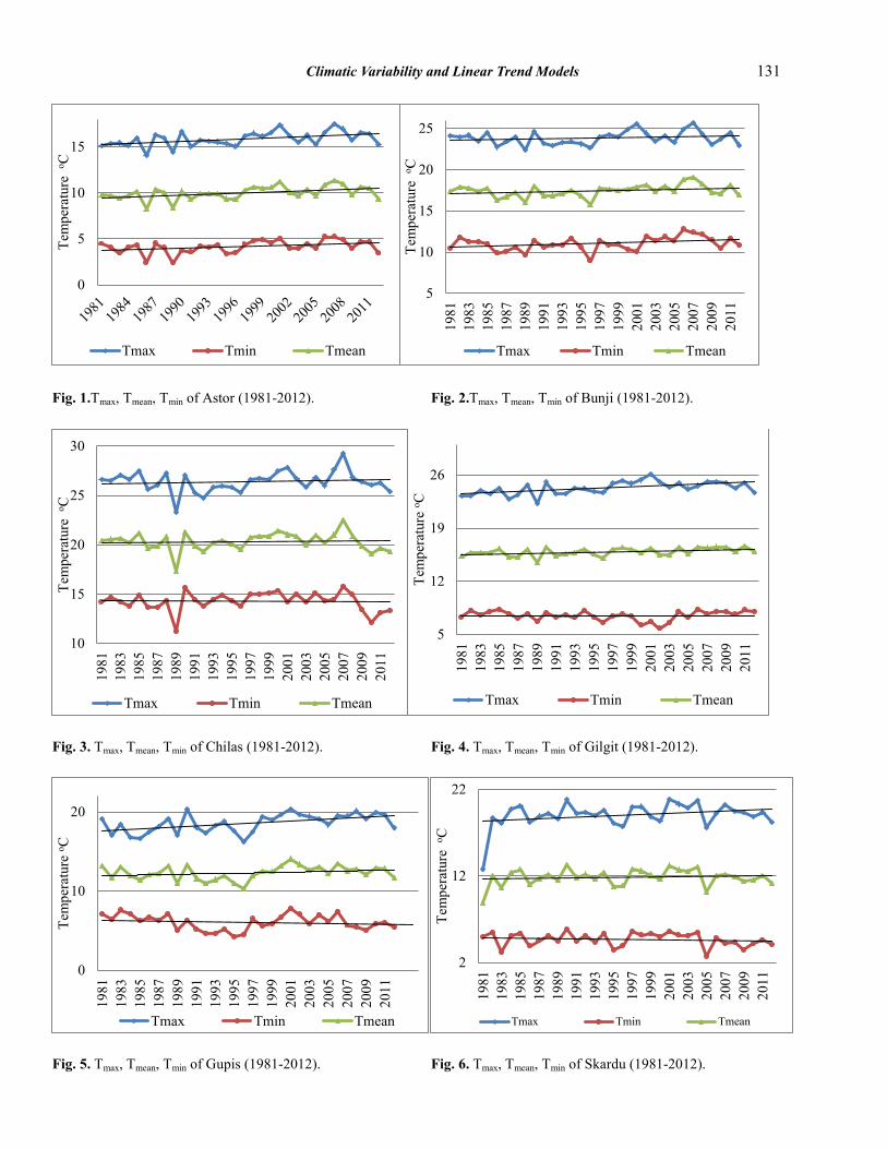
Climatic Variability and Linear Trend Models 131
Fig. 1.Tmax, Tmean, Tmin of Astor (1981-2012). Fig. 2.Tmax, Tmean, Tmin of Bunji (1981-2012).
Fig. 3. Tmax, Tmean, Tmin of Chilas (1981-2012). Fig. 4. Tmax, Tmean, Tmin of Gilgit (1981-2012).
Fig. 5. Tmax, Tmean, Tmin of Gupis (1981-2012). Fig. 6. Tmax, Tmean, Tmin of Skardu (1981-2012).
0
5
10
15
Tem
pera
ture
o C
Tmax Tmin Tmean
5
10
15
20
25
1981
1983
1985
1987
1989
1991
1993
1995
1997
1999
2001
2003
2005
2007
2009
2011
Tem
pera
ture
o C
Tmax Tmin Tmean
10
15
20
25
30
1981
1983
1985
1987
1989
1991
1993
1995
1997
1999
2001
2003
2005
2007
2009
2011
Tem
pera
ture
o C
Tmax Tmin Tmean
5
12
19
2619
8119
8319
8519
8719
8919
9119
9319
9519
9719
9920
0120
0320
0520
0720
0920
11
Tem
pera
ture
o C
Tmax Tmin Tmean
0
10
20
1981
1983
1985
1987
1989
1991
1993
1995
1997
1999
2001
2003
2005
2007
2009
2011
Tem
pera
ture
o C
Tmax Tmin Tmean
2
12
22
1981
1983
1985
1987
1989
1991
1993
1995
1997
1999
2001
2003
2005
2007
2009
2011
Tem
pera
ture
o C
Tmax Tmin Tmean

132 Muhammad Raza et al
The linear (2.1) and quadratic (2.4) trend models were investigated by using least square assessment. 𝑦𝑦 = 𝑎𝑎𝑎𝑎 + 𝑏𝑏 2.1 Where
𝑎𝑎 = ∑𝑦𝑦𝑖𝑖.∑𝑥𝑥𝑖𝑖2−∑𝑥𝑥𝑖𝑖.∑𝑥𝑥𝑖𝑖𝑦𝑦𝑖𝑖
𝑛𝑛.∑𝑥𝑥𝑖𝑖2−(∑𝑥𝑥𝑖𝑖)2
2.2
𝑏𝑏 = 𝑛𝑛∑𝑦𝑦𝑖𝑖𝑥𝑥𝑖𝑖−∑𝑥𝑥𝑖𝑖−∑𝑥𝑥𝑖𝑖.∑𝑦𝑦𝑖𝑖𝑛𝑛.∑𝑥𝑥𝑖𝑖
2−(∑𝑥𝑥𝑖𝑖)2 2.3
xi is the years in the time series such as xo = 1981 (the first year in the time series), whereas yiis the weather parameters (mean, maximum, minimum temperature and annual precipitation). All summations run through i = 0, 1, 2, 3,…..32, i.e., a total of 32 years. Equations 2.2 and 2.3 are the solution of the normal equations related to the scheme. and
𝑦𝑦 = 𝑎𝑎𝑎𝑎2 + 𝑏𝑏𝑎𝑎 + 𝑐𝑐 (2.4)
In this equation, a, b and c are again the solution of normal equations related to the scheme. The obtained linear fit for the given period determine the concern climatic dynamics. The quality of these fittings are further assessed by using some statistical parameters in time series for each case. Which include; Mean Absolute Percentage Error (MAPE), is the measures of accuracy of fitted time series values. Which expresses accuracy in percentage. Its mathematical expression is given by:
𝑀𝑀𝑀𝑀𝑀𝑀𝑀𝑀 = ∑ |(𝑦𝑦𝑡𝑡−𝑦𝑦𝑡𝑡/) 𝑦𝑦𝑡𝑡� |𝑛𝑛
𝑖𝑖=1𝑛𝑛
(2.5)
Where yt is the actual values, y/t is the values
forecast by the models and n is the number of data values. The second parameter is Mean Absolute Deviation (MAD), measure the accuracy of fitted time series. It expresses accuracy in the same units as data, and helps to conceptualize the error. It is computed by using;
𝑀𝑀𝑀𝑀𝑀𝑀 = ∑ |(𝑦𝑦𝑡𝑡−𝑦𝑦𝑡𝑡/)|𝑛𝑛
𝑖𝑖=1𝑛𝑛
(2.6)
The parameter is Root Mean Square Deviation (RMSD), is the measure of accuracy of fitted time series values. RMSD is compute by using the same denominator ‘n’ irrespective of model, we
can compare RMSD values across models. It is computed by using:
𝑅𝑅𝑀𝑀𝑅𝑅𝑀𝑀 = �∑ (𝑦𝑦𝑡𝑡−𝑦𝑦𝑡𝑡/)2𝑛𝑛
𝑖𝑖=1𝑛𝑛
(2.7)
The temperature is analyzed by linear least square estimation, however the precipitation was analyzed through both linear and quadratic models. 3. RESULTS This study reveals that the temperature is increasing, as shown in Table 1. The mean (Tmean), mean minimum (Tmin) and maximum (Tmax) temperature follows an increasing trend that signifies the impact of global warming over GB. Results of linear trends are summarized in Table 1 and main features are conferred below: The increasing rate of maximum temperature of Gup is more than the rest, i.e., 0.065oC/year (Fig. 13a). But the minimum temperature of Gup is, Skardu and Chilas are showing decreasing trend, having values -0.018oC, -0.016oC and -0.002oC/year, respectively. The mean temperature of the most region have an increasing rates that lies within 0.01oC to 0.04oC/year. The minimum temperature of Gilgit has not changed significantly but maximum temperature has been increasing at the rate of 0.05oC/year, as it is evident from Table 1. An in depth trend analysis of precipitation specifies that Gup is received heavy precipitation during number of years under the study period, showing increasing trend significantly. The rate of increase leads the rest with a value 7.001mm/year. This may be one of the possible reasons for decrease in the mean minimum temperature. However quadratic trend analysis shows no significant improvement in the results so linear trend analysis is adequate to extract tendency of temperature. That is why the result are not reported. Generally it is an anticipation that the consequence of global warming is an increase in precipitation in South Asia. This concept also confirm by the result obtain in this study, and all the regions an increase in annual precipitation except Astor and Skardu. The decrease of precipitation 2.655 mm/year and 1.605 mm/year (Fig. 13b) simultaneously in Astor and Skardu. It is a notable feature that may be caused by other latent factors that needs to further explored. Along
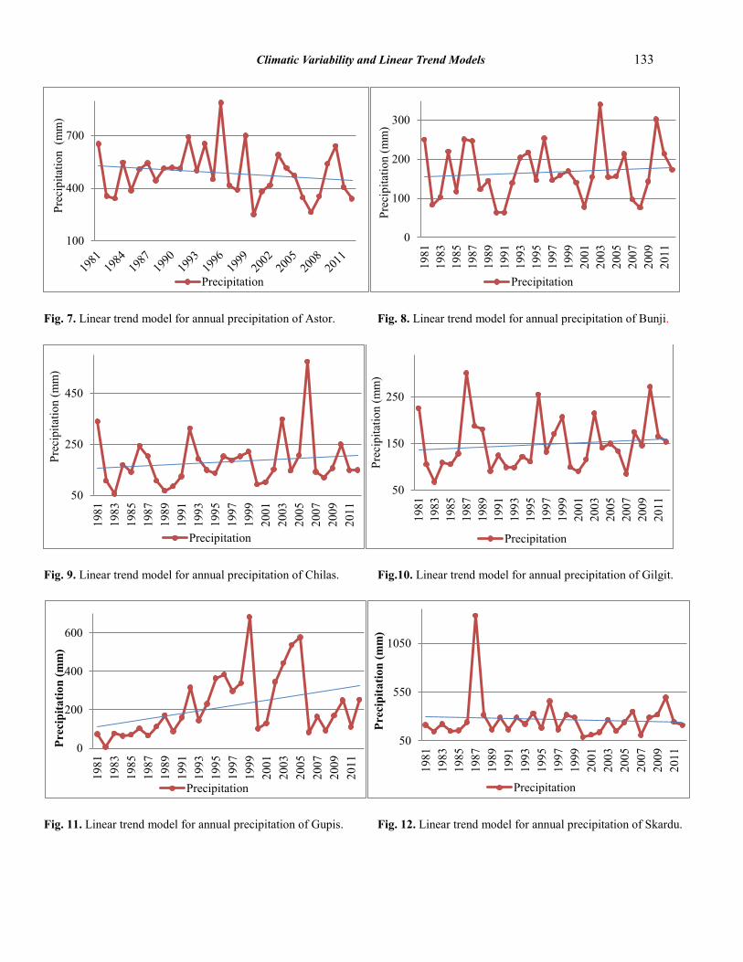
Climatic Variability and Linear Trend Models 133
Fig. 7. Linear trend model for annual precipitation of Astor. Fig. 8. Linear trend model for annual precipitation of Bunji.
Fig. 9. Linear trend model for annual precipitation of Chilas. Fig.10. Linear trend model for annual precipitation of Gilgit.
Fig. 11. Linear trend model for annual precipitation of Gupis. Fig. 12. Linear trend model for annual precipitation of Skardu.
100
400
700
Prec
ipita
tion
(mm
)
Precipitation
0
100
200
300
1981
1983
1985
1987
1989
1991
1993
1995
1997
1999
2001
2003
2005
2007
2009
2011
Prec
ipita
tion
(mm
)
Precipitation
50
250
450
1981
1983
1985
1987
1989
1991
1993
1995
1997
1999
2001
2003
2005
2007
2009
2011
Prec
ipita
tion
(mm
)
Precipitation
50
150
250
1981
1983
1985
1987
1989
1991
1993
1995
1997
1999
2001
2003
2005
2007
2009
2011
Prec
ipita
tion
(mm
)
Precipitation
0
200
400
600
1981
1983
1985
1987
1989
1991
1993
1995
1997
1999
2001
2003
2005
2007
2009
2011
Prec
ipita
tion
(mm
)
Precipitation
50
550
1050
1981
1983
1985
1987
1989
1991
1993
1995
1997
1999
2001
2003
2005
2007
2009
2011
Prec
ipita
tion
(mm
)
Precipitation

134 Muhammad Raza et al
with the linear trend analysis the quadratic least square estimates have also been studied in order to obtain more convergent results. The quadratic fitting results found marginally better than the linear one as given in Table 2. But in-depth analysis of precipitation show that Skardu received record heavy precipitation in 1987 (Fig.12). The rate of increment of
precipitation in Bunji and Gilgit shows approximately same trend (Fig.13b). DISCUSSION The assessment of climate change fundamentally encompasses a good understanding of temperature and precipitation patterns. While studying climate change there are many factors to be considered.
Table 1. Linear Trend equations for mean, maximum & minimum temperature along with MAPE, MAD and RMSD values for major regions of GB.
Region Temp Linear Trend MAPE MAD RMSD
Astor Mean yt=0.036t+9.444 0.054 0.541 0.693 Max yt=0.034t+15.27 0.038 0.613 0.738 Min yt=0.028t+3.668 0.154 0.624 0.751
Bunji Mean yt=0.04t+16.86 0.030 0.521 0.683 Max yt=0.017t+23.53 0.027 0.654 0.801 Min yt=0.03t+10.51 0.057 0.639 0.808
Chilas Mean yt=0.006t+20.22 0.033 0.672 0.896 Max yt=0.015t+26.13 0.028 0.736 1.024 Min yt= -0.002t+14.31 0.049 0.679 0.934
Gilgit Mean yt=0.025t+15.45 0.026 0.419 0.497 Max yt=0.050t+23.44 0.029 0.698 0.874 Min yt=0.00t+7.472 0.069 0.500 0.625
Gupis Mean yt=0.023t+11.93 0.056 0.695 0.837 Max yt=0.065t+11.49 0.051 0.930 1.080 Min yt=-0.018t+6.362 0.143 0.806 0.970
Skardu Mean yt=0.010t+11.68 0.061 0.698 0.917 Max yt=0.046t+18.27 0.049 0.864 1.363 Min yt=-0.016t+4.927 0.155 0.628 0.789
Table 2. Linear and quadratic trend equations of annual precipitation along with MAPE, MAD and RMSD values for major regions of GB. Region Precipitation Linear & Quadratic Trend MAPE MAD RMSD
Astor Yearly yt =-2.655t+528.6 2.474 1243.366 1341.103 yt =-0.390t2+10.22t+455.6 178.836 94113.220 109926.397
Bunji Yearly yt =0.742t+154.5 0.858 111.455 112.833 yt =0.091t2 -2.288t+171.7 13.134 2578.934 3345.105
Chilas Yearly yt =1.674t+154.5 1.743 277.273 285.294 yt =0.018t2+1.050t+158.0 4.422 943.162 1423.615
Gilgit Yearly yt =0.751t+136.1 0.792 99.104 100.101 yt =0.082t2 -1.965t+151.5 10.377 1783.657 2331.241
Gupis Yearly yt =7.001t+102.9 7.293 1414.126 1727.684 yt =-1.006t2+40.21t-85.24 262.093 84638.94 142390.374
Skardu Yearly yt =-1.605t+296.4 1.2195 412.780 688.165 yt =0.035t2-2.780t+303.0 5.001 2906.547 10233.344

Climatic Variability and Linear Trend Models 135
The linear behavior of increasing temperature in all regions except minimum temperature of Gup is and Skardu (Fig. 13b), show a clear effect of global warming in these regions (Table 1). During the study period (i.e., 1981-2012), the region of GB has warmed up by approximately 1.3oC. However, Rasul et al. [4] reported an increase of 1.5oC; similarly results were reported by Raza et al. [15]. This warming trend will greatly affect the seasonal pattern and solid water reservoirs of GB, which is alarm for the consistent flow of water in Indus River. It follows from above conclusion that
GB, as the other parts of Pakistan is also facing land and atmosphere problems by global warming. The effects of global warming on the rainfall are showing up day by day [3]. The precipitation trend of major region of GB is follow highly non-linear, so it is difficult to determine the precipitation pattern by only linear trend analysis as seen from the values of MAPE, MAD and RMSD. That is why we employed quadratic trend analysis that yields better results; their comparisons are given in Table 2. Both Fig. 7 and
Fig. 13(a). Temperature increment per annum for considered areas.
Fig. 13(b). Precipitation increment per annum for considered areas.
0.023
0.01 0.006
0.025
0.036
0.04
0.065
0.046
0.015
0.05 0.034
0.017
-0.018 -0.016
-0.002 0
0.028 0.03
-0.04
-0.02
0
0.02
0.04
0.06
0.08
Gupis Skardu Chilas Gilgit Astor Bunji
Tem
pera
ture
(I
ncre
men
t/yea
r)
Rising Temp Profile (1981-2012)
Mean Max Min
-2.655 -1.605
0.742 0.751
1.674
7.001
-4
-2
0
2
4
6
8
Astor Skardu Bunji Gilgit Chilas GupisPrec
ipita
tion
(Inc
rem
ent/y
ear)
Incresing Precipitation (1981-2012)
136 Muhammad Raza et al
12 shows a negative slope of precipitation pattern for Astor and Skardu sites. To detect precipitation trend more accurately, more sophisticated techniques such as ARIMA modeling and Neural Network must be considered. Moreover the nonlinearities within the data can be dealt by using windowing and space-time separation plots techniques. It is dire need to identify and explain the unexpected behavior of Tmin of Gupis, Skarduand Chilas, as well as annual precipitation pattern of Astor and Skardu. 4. ACKNOWLEDGEMENTS The authors are thankful to Pakistan Meteorological Department (PMD), Islamabad for providing the data and support for this research.
5. REFERENCES
1. Hussain, S.S., M. Mudasser, M.M. Sheikh & N.
Manzoor, Climate change and variability in mountain regions of Pakistan: Implications for water and agriculture. Pakistan Journal of Meteorology 2 (4): 75-90(2005).
2. Stocker, T.F., D. Qin, G.K. Plattner, M. Tignor, S.K. Allen, J. Boschung, A. Nauels, Y. Xia, V. Bex & P.M. Midgley. IPCC, Climate Change 2013: The Physical Science Basis. Contribution of Working Group I to the Fifth Assessment Report of the Intergovernmental Panel on Climate Change. Cambridge University Press, Cambridge, UK (2013).
3. Sadiq, N., & M.S. Qureshi. Climatic variability and linear trend models for the five major cites of Pakistan. Journal of Geography and Geology 2 (1): 83-92 (2010).
4. Rasul, G., A. Mahmood, A. Sadiq, & S.I. Khan. Vulnerability of the Indus Delta to climate change in Pakistan. Pakistan Journal of Meteorology 8(16): 89-107 (2012).
5. David, A., & Freedman. Statistical Models, Theory and Practice. Cambridge University Press, p. 26 (2009).
6. Yan, X. Linear Regression Analysis, Theory and Computing. World Scientific, p. 1-2 (2009).
7. Chaudhary, Q.Z., & G. Rasul. Climatic classification of Pakistan. Journal of Science Vision 9 (1-2 & 3-4): 59-66 (2003, 2004).
8. Chaudhry, Q.Z., A. Mahmood, G. Rasul. & M. Afzaal. Climate Change Indicators of Pakistan. Pakistan Meteorological Department, Islamabad, Pakistan (2009).
9. Solomon, S., D. Qin, M. M anning, Z. Chen, & M. Marquis. Intergovernmental panel on climate change (IPCC), In: Climate Change 2007: The Physical Science Basis. Contribution of Working Group 1 to the Fourth Assessment Report of the Intergovernmental Panel on Climate Change. Cambridge University Press, UK (2007).
10. Landsberg, H.E. Sahel drought change of climate or part of climate. Arch. Met. Geophy. Bioklim. Scr. B. 23: 193-200 (1975).
11. Plummer, N., M.J. Salinger, N. Nicholls, R. Suppiah, K.J. Hennessy, R.M. Leighton, B. Trewin, C.M. Page, & J.M. Lough. Changes in climate extremes over the Australian region and New Zealand during the twentieth century. Climatic Change 42: 183-202 (1999).
12. Pyke, C. Habitat loss confounds climate change impacts. Frontiers in Ecology and the Environment 2(4): 178–182 (2004).
13. Rasul, G., Q.Z. Chaudhry, S.X. Zhao, Q.C. Zeng & G.Y. Zhang. Diagnostic analysis of a heavy rainfall event in South Asia. Journal of Advance in Atmospheric Sciences 22(3): 375-391 (2005).
14. Rao, P.G. Climate changes and trends over a major river basin in India. Climate Research 2: 215-223 (1993).
15. Raza, M., D. Hussain, G. Rasul, M. Akbar & G. Raza. Variations of surface temperature and precipitation in Gilgit-Baltistan (GB), Pakistan from 1955to 2010.Journal of Biodiversity and Environmental Sciences 6(2): 67-73 (2015).

Proceedings of the Pakistan Academy of SciencesInstructions for Authors
Aims and Scope: Proceedings of the Pakistan Academy of Sciences is official journal of the Academy, published quarterly, in English. This open access journal publishes research papers in Engineering Sciences & Technology, Life Sciences, Medical Sciences, and Physical Sciences. State-of-the-art reviews (~20 pages, supported by recent references) summarizing R&D in a particular area of science, especially in the context of Pakistan, and suggesting further R&D are also considered. Manuscripts undergo double-blind review. Authors are not required to be Fellows or Members of the Pakistan Academy of Sciences or citizens of Pakistan.Manuscript FormatManuscript may contain Abstract, Keywords, INTRODUCTION, MATERIALS AND METHODS, RESULTS, DISCUSSION (or RESULTS AND DISCUSSION), CONCLUSIONS, ACKNOWLEDGEMENTS and REFERENCES and any other information that the author(s) may consider necessary. The Manuscript sections must be numbered, i.e., 1. INTRODUCTION, 2. MATERIALS AND METHODS, and so on. Manuscripts, in Times New Roman, 1.5-spaced (but single-space the Tables), with line numbering and one-inch margins on all sides on A-4 size paper, should not exceed 20 pages including Tables and Figures. Number manuscript pages throughout. The text (in Font Size 11, except for the sections mentioned in Font Size 10) must be typed in a single column across the paper width. All Tables and Figures must be placed after the text, i.e., after REFERENCES section.Title Page: For Online submission of the manuscript, Title Page should not be included. However, for submitting as an email attachment, the title page must be as under:(a) Title of the article (Capitalize initial letter of each main word; font size 16; bold), max 160 characters (no abbreviations or acronyms), depicting article’s contents; (b) Author’ first name, middle initial and last name (font size 12, bold), and professional affiliation (i.e., each author’s Department, Institution, Mailing address and Email; but no position titles) (font size 12); (c) Indicate the corresponding author with *; (d) Short running title, max 50 characters ( font size 10).The next Page should start with Title of the Article, followed by entire manuscript. Headings and Subheadings (font size 11): All flush left LEVEL-1: ALL CAPITAL LETTERS; bold Level-2: Capitalize each main word; bold Level-3: Capitalize each main word; Bold, Italic Level-4: Run-in head; Italics, in the normal paragraph position. Capitalize the initial word only and end in a
colon (i.e., :)Abstract (font size 10; max 250 words): Must be self-explanatory, stating rationale, objective(s), methodology, main results and conclusions of the study. Abbreviations, if used, must be defined on first mention in the Abstract as well as in the main text. Abstract of review articles may have variable format.
Keywords (font size 10): Three to eight keywords, depicting the article.
For Online submission: • Separate submission of Abstract along with Title is required• Author(s)’namesandaffiliationsshouldnotbeincludedinthemanuscriptortheAbstract
INTRODUCTION: Provide a clear and concise statement of the problem, citing relevant recent literature, and objectives of the investigation.MATERIALS AND METHODS: Provide an adequate account of the procedures or experimental details, including statistical tests (if any), in a concise manner but sufficient enough to replicate the study. RESULTS: Be clear and concise with the help of appropriate Tables, Figures and other illustrations. Data should not be repeated in Tables and Figures, but must be supported with statistics.DISCUSSION: Provide interpretation of the RESULTS in the light of previous relevant studies, citing published references. ACKNOWLEDGEMENTS (font size 10): In a brief statement, acknowledge financial support and other assistance.REFERENCES (font size 10): Cite references in the text by number only in square brackets, e.g. “Brown et al [2]

138
reported ...” or “... as previously described [3, 6 –8]”, and list them in REFERENCES section, in the order of citation in the text, Tables and Figures (not alphabetically). Only published (and accepted for publication) journal articles, books, and book chapters qualify for REFERENCES. List of REFERENCES must be prepared as under:a. Journal Articles (Name of journals must be stated in full)
1. Golding, I. Real time kinetics of gene activity in individual bacteria. Cell 123: 1025–1036 (2005).2. Bialek, W. & S. Setayeshgar. Cooperative sensitivity and noise in biochemical signaling. Physical Review
Letters 100: 258–263 (2008).3. Kay, R.R. & C.R.L. Thompson. Forming patterns in development without morphogen gradients: differentiation
and sorting. Cold Spring Harbor Perspectives in Biology 1: doi: 10.1101/cshperspect.a001503 (2009).b. Books
4. Luellen, W.R. Fine-Tuning Your Writing. Wise Owl Publishing Company, Madison, WI, USA (2001).5. Alon, U. & D.N. Wegner (Ed.). An Introduction to Systems Biology: Design Principles of Biological Circuits.
Chapman & Hall/CRC, Boca Raton, FL, USA (2006).c. Book Chapters
6. Sarnthein, M.S. & J.D. Stanford. Basal sauropodomorpha: historical and recent phylogenetic developments. In: The Northern North Atlantic: A Changing Environment. Schafer, P.R. & W. Schluter (Ed.), Springer, Berlin, Germany, p. 365–410 (2000).
7. Smolen, J.E. & L.A. Boxer. Functions of Europhiles. In: Hematology, 4th ed. Williams, W.J., E. Butler & M.A. Litchman (Ed.), McGraw Hill, New York, USA, p. 103–101 (1991).
Tables, with concise but self-explanatory headings must be numbered according to the order of citation (like Table 1, Table 2). Round off data to the nearest three significant digits. Provide essential explanatory footnotes, with superscript letters or symbols keyed to the data. Do not use vertical or horizontal lines, except for separating column heads from the data and at end of the Table. Figures may be printed in two sizes: column width of 8.0 cm or page width of 16.5 cm; number them as Fig. 1, Fig. 2, … in the order of citation in the text. Captions to Figures must be concise but self-explanatory. Laser printed line drawings are acceptable. Do not use lettering smaller than 9 points or unnecessarily large. Photographs must be of high quality. A scale bar should be provided on all photomicrographs. Declaration: Provide a declaration that: (i) the results are original; (ii) the same material is neither published nor under consideration elsewhere; (iii) approval of all authors has been obtained; and, (iv) in case the article is accepted for publication, its copyright will be assigned to Pakistan Academy of Sciences. Authors must obtain permission to reproduce, where needed, copyrighted material from other sources and ensure that no copyrights are infringed upon.
Reviewers: Authors may suggest four relevant reviewers, two local and two from scientifically advanced countries.
Online Manuscript Submission:Proceedings of the Pakistan Academy of Sciences is using a web-enabled online manuscript submission and review system, which offers authors the option to track the progress of manuscripts in real time. For online submission, authors are required to register at website of the Academy (www.paspk.org) by clicking the “Journal and Publications” tab. Manuscripts must be submitted in Microsoft Word (.doc or .docx format; pdf files not acceptable). Figures can be submitted in Word format, TIFF, GIF, JPEG, EPS, PPT.NOTE: In case of online submission, authors are not required to submit the manuscript as email attachment. In case of any difficulty while submitting your manuscript, please get in touch with:
Editor-in-Chief Pakistan Academy of Sciences3-Constitution Avenue, G-5/2, Islamabad, Pakistan
Email: [email protected] Tel: +92-51-920 7140 Website: www.paspk.org
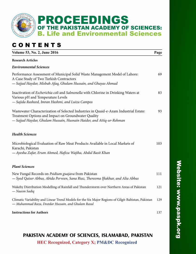
C O N T E N T SVolume 53, No. 2, June 2016 Page
Research Articles
Environmental Sciences
Performance Assessment of Municipal Solid Waste Management Model of Lahore: 69A Case Study of Two Turkish Contractors— Sajjad Haydar, Misbah Afaq, Ghulam Hussain, and Ghayas Ahmad
Inactivation of Escherichia coli and Salmonella with Chlorine in Drinking Waters at 83Various pH and Temperature Levels— Sajida Rasheed, Imran Hashmi, and Luiza Campos
Wastewater Characterization of Selected Industries in Quaid-e-Azam Industrial Estate: 93Treatment Options and Impact on Groundwater Quality— Sajjad Haydar, Ghulam Hussain, Husnain Haider, and Attiq-ur-Rehman
Health Sciences
Microbiological Evaluation of Raw Meat Products Available in Local Markets of 103Karachi, Pakistan— Ayesha Zafar, Erum Ahmed, Hafiza Wajiha, Abdul Basit Khan
Plant Sciences
New Fungal Records on Psidium guajava from Pakistan 111— Syed Qaiser Abbas, Abida Perveen, Sana Riaz, Thereema Iftakhar, and Alia Abbas
Wakeby Distribution Modelling of Rainfall and Thunderstorm over Northern Areas of Pakistan 121— Naeem Sadiq
Climatic Variability and Linear Trend Models for the Six Major Regions of Gilgit-Baltistan, Pakistan 129— Muhammad Raza, Dostdar Hussain, and Ghulam Rasul
Instructions for Authors 137
HEC Recognized, Category X; PM&DC Recognized
PROCEEDINGSOF THE PAKISTAN ACADEMY OF SCIENCES:B. Life and Environmental Sciences
Website: w
ww
.paspk.org PAKISTAN ACADEMY OF SCIENCES, ISLAMABAD, PAKISTAN