VLSI Architectures for Communications and Signal...
77
1 VLSI Architectures for Communications and Signal Processing Kiran Gunnam IEEE SSCS Distinguished Lecturer Director of Engineering, Violin Memory
-
Upload
trinhtuong -
Category
Documents
-
view
219 -
download
2
Transcript of VLSI Architectures for Communications and Signal...

1
VLSI Architectures for Communications
and Signal Processing
Kiran Gunnam
IEEE SSCS Distinguished LecturerDirector of Engineering, Violin Memory

2
Outline
Part I
� Trends in Computation and Communication
� Basics
� Pipelining and Parallel Processing
� Folding, Unfolding, Retiming, Systolic Architecture Design
Part II
� LDPC Decoder
� Turbo Equalization, Local-Global Interleaver and Queuing
� Error Floor Mitigation (Brief)
� T-EMS (Brief)
VLSI Architectures for Communications and Signal Processing
8/18/2013
3
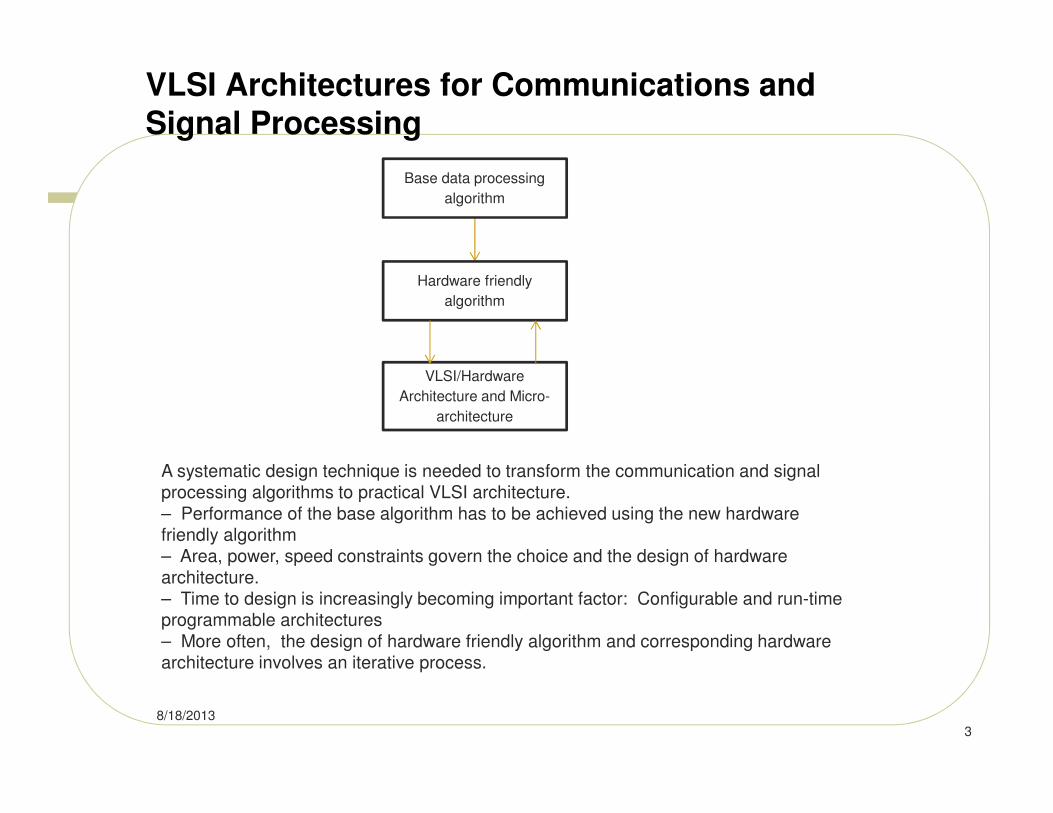
A systematic design technique is needed to transform the communication and signal processing algorithms to practical VLSI architecture.
– Performance of the base algorithm has to be achieved using the new hardware friendly algorithm– Area, power, speed constraints govern the choice and the design of hardware
architecture.– Time to design is increasingly becoming important factor: Configurable and run-time programmable architectures
– More often, the design of hardware friendly algorithm and corresponding hardware architecture involves an iterative process.
Base data processing
algorithm
Hardware friendly
algorithm
VLSI/Hardware
Architecture and Micro-
architecture

Communication and Signal Processing applications
� Wireless Personal Communication – 3G,B3G,4G,...etc.– 802.16e,802.11n,UWB,...etc.
� Digital Video/Audio Broadcasting– DVB-T/H, DVB-S,DVB-C, ISDB-T,DAB,...etc.
� Wired Communications– DSL, HomePlug, Cable modem, etc.
� Storage
� -Magnetic Read Channel, Flash read channel
� Video Compression
� TV setup box
8/18/2013
4
Convergence of Communications and Semiconductor technologies
� High system performance
� – Increase Spectrum efficiency of modem (in bits/sec/Hz/m^3)
• Multi-antenna diversity• Beamforming• Multi-user detection• Multi-input Multi-output (MIMO) Systems • Etc.
� • High silicon integrations– Moore’s Law– High-performance silicon solutions
– Low power and cost
- Mobile devices getting more computation, vision and graphics capabilities
8/18/2013
5
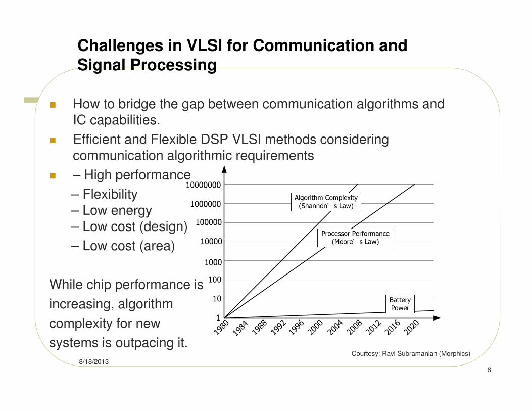
Challenges in VLSI for Communication and Signal Processing
� How to bridge the gap between communication algorithms and IC capabilities.
� Efficient and Flexible DSP VLSI methods considering communication algorithmic requirements
� – High performance
– Flexibility– Low energy– Low cost (design)
– Low cost (area)
While chip performance is
increasing, algorithm
complexity for new
systems is outpacing it.
8/18/2013
6
Courtesy: Ravi Subramanian (Morphics)

8/18/2013
7
FIGURE S.1 Historical growth in single-processor performance and a forecast of processor performance to 2020, based on the ITRS roadmap.
The dashed line represents expectations if single-processor performance had continued its historical trend. The vertical scale is logarithmic. A break in the growth rate at around 2004 can be seen.
Before 2004, processor performance was growing by a factor of about 100 per decade; since 2004, processor performance has been growing and is forecasted to grow by a factor of only about 2 per decade.
In 2010, this expectation gap for single-processor performance is about a factor of 10; by 2020, it will have grown to a factor of 100.
Note that this graph plots processor clock rate as the measure of processor performance. Other processor design choices impact processor performance, but clock rate is a dominant processor performance determinant.
Courtesy: NAE Report, “The Future of Computing Performance:
Game Over or Next Level?”
Single Processor Performance Trends

Scaling Trends
8/18/2013
8
Courtesy: NAE Report, “The Future of Computing Performance:
Game Over or Next Level?”
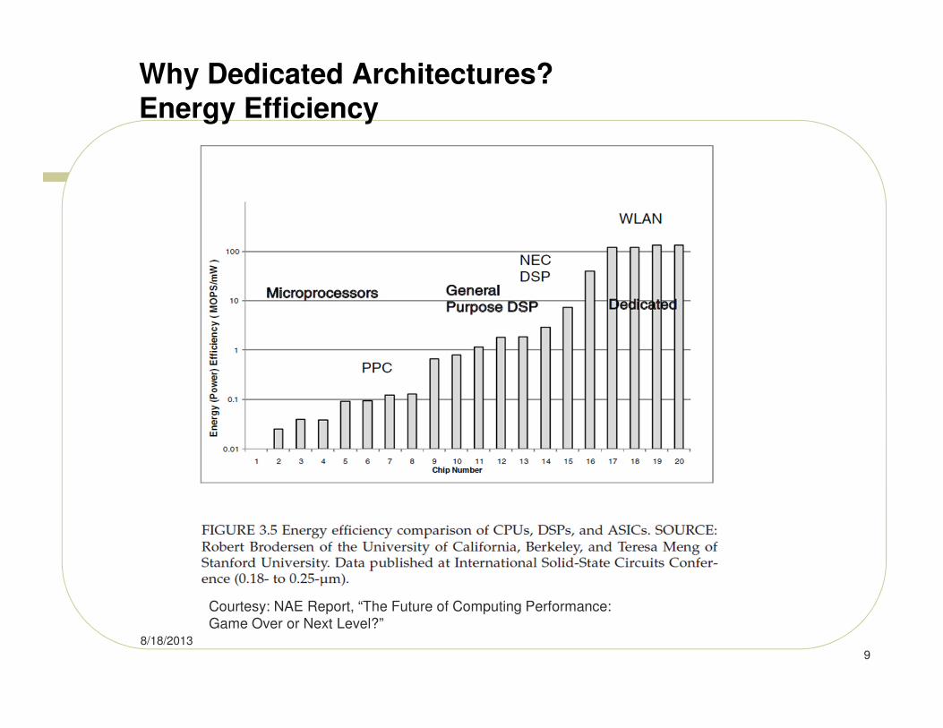
Why Dedicated Architectures? Energy Efficiency
8/18/2013
9
Courtesy: NAE Report, “The Future of Computing Performance:
Game Over or Next Level?”

Why Dedicated Architectures? Area Efficiency
8/18/2013
10
NAE Report Recommendation: “Invest in research and development of parallel architectures
driven by applications, including enhancements of chip multiprocessor systems and conventional
data-parallel architectures, cost effective designs for application-specific architectures, and
support for radically different approaches.”
Courtesy: NAE Report, “The Future of Computing Performance:
Game Over or Next Level?”

8/18/2013 11
Basic Ideas
� Parallel processing � Pipelined processing
a1 a2 a3 a4
b1 b2 b3 b4
c1 c2 c3 c4
d1 d2 d3 d4
a1 b1 c1 d1
a2 b2 c2 d2
a3 b3 c3 d3
a4 b4 c4 d4
P1
P2
P3
P4
P1
P2
P3
P4
time
Colors: different types of operations performed
a, b, c, d: different data streams processed
Can combine parallel processing and pipelining-will have
16 processors instead of 4.
Less inter-processor communication
Complicated processor hardware
time
More inter-processor communication
Simpler processor hardware
Courtesy: Yu Hen Hu

Basic Ideas
8/18/2013
12
Basic micro-architectural techniques: reference architecture (a), and its parallel (b) and
pipelined (c) equivalents. Reference architecture (d) for time-multiplexing (e). Area
overhead is indicated by shaded blocks.
Bora et. al, “Power and Area Efficient VLSI Architectures for Communication
Signal Processing”, ICC 2006

13
8/18/2013
Data Dependence
� Parallel processing requires NO data dependence between processors
� Pipelined processing will involve inter-processor communication
P1
P2
P3
P4
P1
P2
P3
P4
time time
Courtesy: Yu Hen Hu

Folding
14
Concept of folding: (a) time-serial computation, (b) operation folding. Block Alg performs some algorithmic
operation.
Bora et. al, “Power and Area Efficient VLSI Architectures for Communication
Signal Processing”, ICC 2006
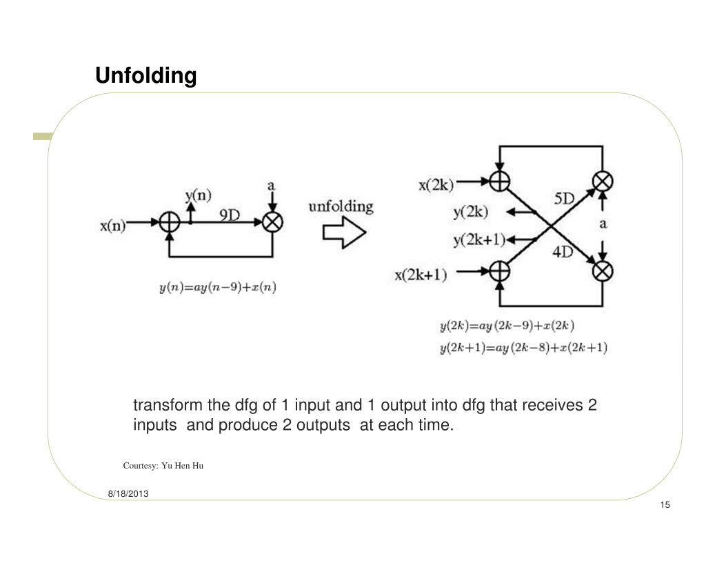
Unfolding
8/18/2013
15
transform the dfg of 1 input and 1 output into dfg that receives 2
inputs and produce 2 outputs at each time.
Courtesy: Yu Hen Hu

16
Block Processing
� One form of vectorizedparallel processing of DSP algorithms. (Not the parallel processing in most general sense)
� Block vector: [x(3k) x(3k+1) x(3k+2)]
� Clock cycle: can be 3 times longer
� Original (FIR filter):
� Rewrite 3 equations at a time:
� Define block vector
� Block formulation:
(3 ) (3 ) (3 1) (3 2)
(3 1) (3 1) (3 ) (3 1)
(3 2) (3 2) (3 1) (3 )
y k x k x k x k
y k a x k b x k c x k
y k x k x k x k
− −
+ = + + + − + + +
( ) ( ) ( 1)
( 2)
y n a x n b x n
c x n
= ⋅ + ⋅ −
+ ⋅ −
(3 )
( ) (3 1)
(3 2)
x k
k x k
x k
= + +
x
0 0 0
( ) 0 ( ) 0 0 ( 1)
0 0 0
a c b
k b a k c k
c b a
= + −
y x x
Courtesy: Yu Hen Hu

Systolic Architectures
17
Matrix-like rows of data processing units called cells.
Transport Triggered.
Matrix multiplication C=A*B.
A is fed in a row at a time from the top of the array and is passed down the
array,
B is fed in a column at a time from the left hand side of the array and passes
from left to right.
Dummy values are then passed in until each processor has seen one whole row
and one whole column.
The result of the multiplication is stored in the array and can now be output a
row or a column at a time, flowing down or across the array.
Figure by Rainier

LDPC DECODER
8/18/2013
18

19
Requirements for Wireless systems and Storage Systems
Magnetic Recording systems� Data rates are 3 to 5 Gbps.� Real time BER requirement is 1e-10 to 1e-12� Quasi real-time BER requirement is 1e-15 to 1e-18� Main Channel impairments: ISI+ data dependent noise (jitter)
+ erasures � Channel impairments are getting worse with the increasing recording densities.
Wireless Systems: � Data rates are 0.14 Mbps (CDMA 2000) to 326.4 Mbps (LTE UMTS/4GSM) .� Real time BER requirement is 1e-6� Main Channel impairments: ISI (frequency selective channel) � + time varying fading channel� + space selective channel
+ deep fades � Increasing data rates require MIMO systems and more complex channel estimation and receiver
algorithms
In general the algorithms used in wireless systems and magnetic recording systems are similar. The increased complexity in magnetic recording system stems from increased data rates while the SNR requirements are getting tighter.
For ISI channels, the near optimal solution is turbo equalization using a detector and advanced ECC such as LDPC.
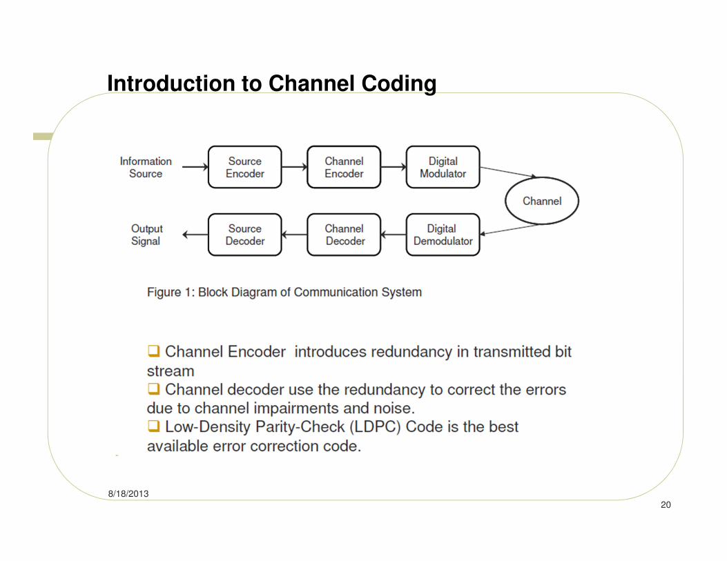
Introduction to Channel Coding
8/18/2013
20

Some Notation and Terminology
8/18/2013
21
Courtesy: Dr. Krishna Narayanan (Texas A&M)

Shannon Capacity and Channel Codes
� The Shannon limit or Shannon capacity of a communications
channel is the theoretical maximum information transfer rate of the
channel, for a particular noise level.
� Random and long code lengths achieve channel capacity.
� To construct a random code, pick 2k codewords of length n at
random. Code is guaranteed to be good as k!
� Decoding random codes, require storage of 2k codewords
� There are only about 1082 (~ 2276) atoms in the universe.
� Encoding/Decoding complexities don’t increase drastically with k
� Storage does not increase drastically with k
� Randomness Vs Structure
� Random codes are good
� But structure is needed to make it practical
8/18/2013
22
Courtesy: Dr. Krishna Narayanan (Texas A&M)
Coding Theory Advances
� There are two kinds of codes: Block Codes and Convolutional
codes
� Block Codes: In an (n,k) block code, k bits are encoded in to n bits.
Block code is specified by k x n generator matrix G or an (n-k) x n
parity check matrix H
� Examples: Hamming, BCH, Reed Solomon Codes. Hard decision
decoding is used. Soft decoding possible- but complex.
� Convolutional codes: Can encode infinite sequence of bits using
shift registers. Soft decision decoding such as viterbi can achieve
optimal maximum likelihood decoding performance.
� Turbo Codes (1993): Parallel concatenated convolutional codes.
� Rediscovery: LDPC Block code(1962, 1981, 1998). Near shannon
limit code, Efficient soft decoding (message passing) and with
iterations.
8/18/2013
23

Progress in Error Correction Systems
8/18/2013
24

25
LDPC Decoding, Quick Recap, 1/5
Variable nodes correspond to the soft information of received bits.
Check nodes describe the parity equations of the transmitted bits.
eg. v1+v4+v7= 0; v2+v5+v8 =0 and so on.
The decoding is successful when all the parity checks are satisfied (i.e. zero).

• There are four types of LLR messages
• Message from the channel to the n-th bit node,
• Message from n-th bit node to the m-th check node or simply
• Message from the m-th check node to the n-th bit node or simply
• Overall reliability information for n-th bit-node
26
( )i
n mQ − >
( )i
m nR − >
nL
nP
Channel Detector
L3
Channel Detector
m = 2m = 1m = 0
32 >−R(i)
30 >−R(i)
)(
13
iQ >−
6P
n = 0 n = 1 n = 2 n = 3 n = 4 n = 5 n = 6
( )i
nmQ
( )i
m nR
LDPC Decoding, Quick Recap, 2/5
Courtesy: Ned Varnica

8/18/2013
27
Notation used in the equations
nx is the transmitted bit n ,
nL is the initial LLR message for a bit node (also called as variable node) n ,
received from channel/detector
nP is the overall LLR message for a bit node n ,
nx)
is the decoded bit n (hard decision based on nP ) ,
[Frequency of P and hard decision update depends on decoding schedule]
)(nΜ is the set of the neighboring check nodes for variable node n ,
)(mΝ is the set of the neighboring bit nodes for check node m .
For the ith
iteration, ( )i
nmQ is the LLR message from bit node n to check node m ,
( )i
mnR is the LLR message from check node m to bit node n .
LDPC Decoding, Quick Recap, 3/5
8/18/2013
28
(A) check node processing: for each m and )(mn Ν∈ ,
( ) ( ) ( )i
mn
i
mn
i
mnR κδ= (1)
( )
( )
( )( ) 1min
\
i i
mn mn
iR Q
n mn m nκ
−= =
′′∈ Ν
(2)
The sign of check node message( )i
mnR is defined as
( ) ( )( )( )
1
\
sgni i
mn n m
n m n
Qδ−
′
′∈Ν
=
∏ (3)
where( )i
mnδ takes value of 1+ or 1−
LDPC Decoding, Quick Recap, 4/5

8/18/2013
29
(B) Variable-node processing: for each n and ( )m M n∈ :
( ) ( )
( )\
i i
nm n m n
m n m
Q L R ′
′∈Μ
= + ∑ (4)
(C) P Update and Hard Decision ( )
( )
i
n n mn
m M n
P L R∈
= + ∑ (5)
A hard decision is taken where ˆ 0nx = if 0n
P ≥ , and ˆ 1nx = if 0n
P < .
If ˆ 0T
nx H = , the decoding process is finished with ˆ
nx as the decoder output;
otherwise, repeat steps (A) to (C).
If the decoding process doesn’t end within some maximum iteration, stop and
output error message.
Scaling or offset can be applied on R messages and/or Q messages for better
performance.
LDPC Decoding, Quick Recap, 5/5

8/18/2013
30
Example QC-LDPC Matrix
=
−−−−
−
−
)1)(1(2)1(1
)1(242
12
...
:
...
...
...
rccc
r
r
I
I
I
IIII
H
σσσ
σσσ
σσσ
=
01....00
:
00....10
00...01
10...00
σ Example H Matrix, Array
LDPC
r row/ check node degree=5
c columns/variable node degree=3
Sc circulant size=7
N=Sc*r=35

8/18/2013
31
Example QC-LDPC Matrix
=×
17411675507
14411396645
16514211032
53S
Example H Matrix
r row degree=5
c column degree =3
Sc circulant size=211
N=Sc*r=1055

Decoder Architectures
� Parallelization is good-but comes at a steep cost for LDPC.
� Fully Parallel Architecture:
� All the check updates in one clock cycle and all the bit updates in one more clock cycle.
� Huge Hardware resources and routing congestion.
8/18/2013
32

Decoder Architectures, Serial
� Check updates and bit updates in a serial fashion.
� Huge Memory requirement. Memory in critical path.
8/18/2013
33

Decoder Architectures, Serial
8/18/2013
34

Semi-parallel Architectures
� Check updates and bit updates using several units.
� Partitioned memory by imposing structure on H
matrix.
� There are several semi-parallel architectures
proposed.
� Initial semi-parallel architectures were complex and
very low throughput. Needed huge amounts of
memory.
8/18/2013
35

On-the-fly Computation
Our previous research ([1-13]) introduced the following concepts to LDPC decoder implementation.
References P1-P4 are more comprehensive and are the basis for this presentation.
1. Block serial scheduling
2. Value-reuse,
3. Scheduling of layered processing,
4. Out-of-order block processing,
5. Master-slave router,
6. Dynamic state,
7. Speculative Computation
8. Run-time Application Compiler [support for different LDPC codes with in a class of codes. Class:802.11n,802.16e,Array, etc. Off-line re-configurable for several regular and irregular LDPC codes]
All these concepts are termed as On-the-fly computation as the core of these
concepts are based on minimizing memory and re-computations by employing just
in-time scheduling. For this presentation, we will focus on concept 4.
36

8/18/2013
37
Check Node Unit (CNU) Design
( )
( )
( )( ) 1min
\
i i
m l m l
iR Q
l ml m lκ → →
−= =
′ →′∈ Ν
m
10−=>−
i
mn1Q
L1 L2 L3
133=
>−i
mnQ
52−=
>−i
mnQ
m
-51=>−
i
nmR 53=>−
i
nmR-102=>−
i
nmR
bits to checks checks to bits
L1 L2 L3

Check Node Unit (CNU) Design
The above equation (2) can be reformulated as the following set of equations.
• Simplifies the number of comparisons required as well as the memory
needed to store CNU outputs.
• Additional design choices: The correction has to be applied to only two values instead
of distinct values. Need to apply 2’s complement to only 1 or 2 values instead of
values at the output of CNU.
38
( )
( )
( )11 min
i
m
iM Q
mnn m
−=
′′∈ Ν
(6)
( )
( )
( )12 2 min
i
m
iM nd Q
mnn m
−=
′′∈ Ν
(7)
1k Min Index= (8)
( ) ( )1
i i
mn mMκ = , ( ) kmn \Ν∈∀
( )
2i
mM= , kn = (9)
( )
( )
( )( ) 1min
\
i i
mn mn
iR Q
n mn m nκ
−= =
′′∈ Ν
(2)

CNU Micro Architecture for min-sum
8/18/2013
39
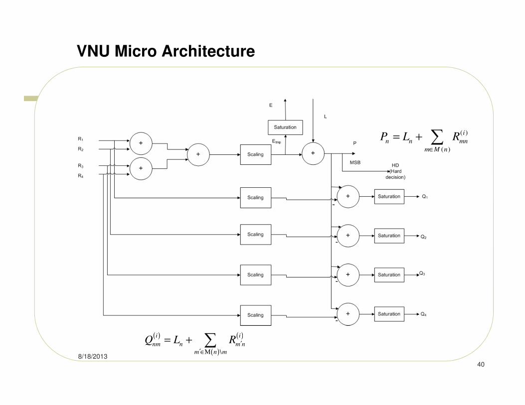
VNU Micro Architecture
8/18/2013
40
( ) ( )
( )\
i i
nm n m n
m n m
Q L R ′
′∈Μ
= + ∑
( )
( )
i
n n mn
m M n
P L R∈
= + ∑

Non-Layered Decoder Architecture
41
L Memory=> Depth 36, Width=128*5
HD Memory=> Depth 36, Width=128
Possible to remove the
shifters (light-blue) by re-
arranging H matrix’s first
layer to have zero shift
coefficients.
Supported H matrix
parameters
r row degree=36
c column degree =4
Sc ciruclant size=128
N=Sc*r=4608

Pipeline for Non-layered Decoder

Layered Decoder Architecture
43
Optimized Layered Decoding with algorithm transformations for reduced memory and computations
)0()0(
, ,0 nnnl LPRrrr
== [Initialization for each new received data frame], (9)
max,,2,1 iti L=∀ [Iteration loop],
1,2, ,l j∀ = L [Sub-iteration loop],
kn ,,2,1 L=∀ [Block column loop],
( )[ ] [ ] ( )1
,
),(),(
,
−−= i
nl
nlS
n
nlSi
nl RPQrrr
, (10)
( ) ( )[ ] ( )( )knQfRnlSi
nl
i
nl ,,2,1,,
,, Lrr
=′∀=′
′ , (11)
[ ] ( )[ ] ( )i
nl
nlSi
nl
nlS
n RQP ,
),(
,
),( rrr+= , (12)
where the vectors ( )i
nlR ,
r and
( )i
nlQ ,
r represent all the R and Q messages in each pp × block of the H matrix,
( , )s l n denotes the shift coefficient for the block in lth block row and n
th block column of the H matrix.
( )[ ] ),(
,
nlSi
nlQr
denotes that the vector ( )i
nlQ ,
r is cyclically shifted up by the amount ( , )s l n
k is the check-node degree of the block row.
A negative sign on ( , )s l n indicates that it is a cyclic down shift (equivalent cyclic left shift).
)(⋅f denotes the check-node processing, which embodiments implement using, for example, a Bahl-Cocke-
Jelinek-Raviv algorithm (“BCJR”) or sum-of-products (“SP”) or Min-Sum with scaling/offset.

Layered Decoder Architecture
44
( )[ ] [ ] ( )1
,
),(),(
,
−−= i
nl
nlS
n
nlSi
nl RPQrrr
( )( )[ ] ( )
=′∀=
′
′
kn
QfR
nlSi
nli
nl
,,2,1
,,
,,
L
rr
[ ] ( )[ ] ( )i
nl
nlSi
nl
nlS
n RQP ,
),(
,
),( rrr+=
Q=P-Rold
Our work proposed this for H matrices with regular
mother matrices.
Compared to other work, this work has several advantages
1) No need of separate memory for P.
2) Only one shifter instead of 2 shifters
3) Value-reuse is effectively used for both Rnew and Rold
4) Low complexity data path design-with no redundant data
Path operations.
5) Low complexity CNU design.

Data Flow Diagram
45

46
Irregular QC-LDPC H Matrices
Flash Memory Summit 2013
Santa Clara, CA 46
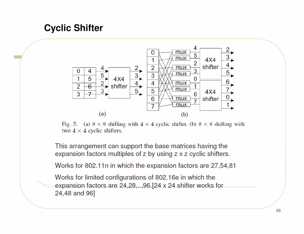
Different base matrices to support different rates.
Different expansion factors (z) to support multiple lengths.
All the shift coefficients for different codes for a given rate are obtained from the
same base matrix using modulo arithmetic

Irregular QC-LDPC H Matrices
47

Irregular QC-LDPC H Matrices
� Existing implementations [Hocevar] for irregular QC-LDPC codes are
still very complex to implement.
� These codes have the better BER performance and selected for IEEE
802.16e and IEEE 802.11n.
� It is anticipated that these type of codes will be the default choice for
most of the standards.
� We show that with out-of-order processing and scheduling of layered
processing, it is possible to design very efficient architectures.
� The same type of codes can be used in storage applications
(holographic, flash and magnetic recording) if variable node degrees
of 2 and 3 are avoided in the code construction for low error floor
48
Hocevar, D.E., "A reduced complexity decoder architecture via layered decoding of LDPC codes,"
IEEE Workshop on Signal Processing Systems, 2004. SIPS 2004. .pp. 107- 112, 13-15 Oct. 2004
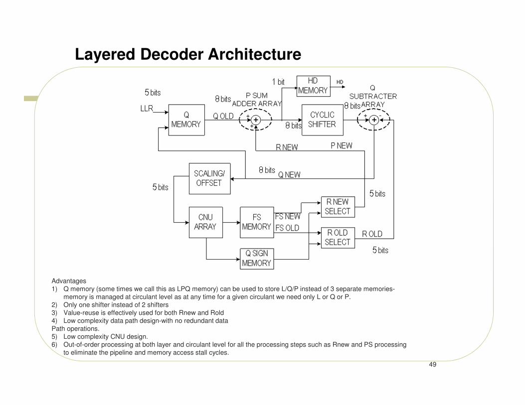
Layered Decoder Architecture
49
Advantages
1) Q memory (some times we call this as LPQ memory) can be used to store L/Q/P instead of 3 separate memories-
memory is managed at circulant level as at any time for a given circulant we need only L or Q or P.
2) Only one shifter instead of 2 shifters
3) Value-reuse is effectively used for both Rnew and Rold
4) Low complexity data path design-with no redundant data
Path operations.
5) Low complexity CNU design.
6) Out-of-order processing at both layer and circulant level for all the processing steps such as Rnew and PS processing
to eliminate the pipeline and memory access stall cycles.

Out-of-order layer processing for R Selection
50
Normal practice is to compute R new messages for each layer after CNU PS processing.
However, here we decoupled the execution of R new messages of each layer with the execution of corresponding
layer’s CNU PS processing. Rather than simply generating Rnew messages per layer, we compute them on basis
of circulant dependencies.
R selection is out-of-order so that it can feed the data required for the PS processing of the second layer. For
instance Rnew messages for circulant 29 which belong to layer 3 are not generated immediately after layer 3
CNU PS processing .
Rather, Rnew for circulant 29 is computed when PS processing of circulant 20 is done as circulant 29 is a
dependent circulant of circulant of 20.
Similarly, Rnew for circulant 72 is computed when PS processing of circulant 11 is done as circulant 72 is a
dependent circulant of circulant of 11.
Here we execute the instruction/computation at precise moment when the result is needed!

Out-of-order block processing for Partial State
51
51
Re-ordering of block processing . While processing the layer 2,
the blocks which depend on layer 1 will be processed last to allow for the pipeline latency.
In the above example, the pipeline latency can be 5.
The vector pipeline depth is 5.so no stall cycles are needed while processing the layer 2 due to the pipelining. [In
other implementations, the stall cycles are introduced – which will effectively reduce the throughput by a huge
margin.]
Also we will sequence the operations in layer such that we process the block first that has dependent data
available for the longest time.
This naturally leads us to true out-of-order processing across several layers. In practice we wont do out-of-order
partial state processing involving more than 2 layers.

Block Parallel Layered Decoder
52
Compared to other work, this work has several advantages
1) Only one memory for holding the P values.
2) Shifting is achieved through memory reads. Only one
memory multiplexer network is needed instead of 2 to achieve
delta shifts
3) Value-reuse is effectively used for both Rnew and Rold
4) Low complexity data path design-with no redundant data
Path operations.
5) Low complexity CNU design with high parallelism.
6) Smaller pipeline depth
7) Out-of-order row processing to hide the pipeline latencies.
Here M is the row parallelization
(i.e. number of rows in H matrix
Processed per clock).
53
Cyclic Shifter

Benes Network
8/18/2013
54
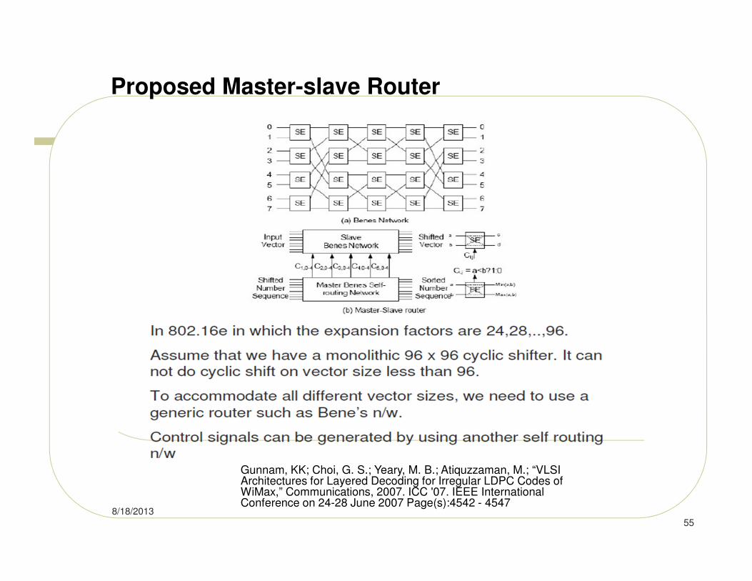
Proposed Master-slave Router
8/18/2013
55
Gunnam, KK; Choi, G. S.; Yeary, M. B.; Atiquzzaman, M.; “VLSI Architectures for Layered Decoding for Irregular LDPC Codes of WiMax,” Communications, 2007. ICC '07. IEEE International Conference on 24-28 June 2007 Page(s):4542 - 4547
Master-slave router
8/18/2013
56

TURBO EQUALIZATION
8/18/2013
57

58
System Model for Turbo Equalization
ky ′
( )kk xL
( )kk xE
kx)
kukx

59
Proposed System Level Architecture for Turbo Equalization
SISODetector(NP-MAP/NP-ML)2x
Interleaver
De-Interleaver
ky ′
kx)
YQueueD/G/1/1+n
LEQueue
G/G/1/1+m
HDQueueG/D/1/1+h
LPQPing-pongMemory
FS QueueG/G/1/1+a
LDPCDecoder Core
SISO LDPC Decoder
Low complexityDetector (Hard Decision VA)D/D/1/1
Preliminary hard decisions to Timing Loops
QueueSchedulingProcessor
Hard Decision LDPC Decoder1 iterationD/D/1/1+1
Hard DecisionDe-Interleaver
kx′
HD Ping-pongMemory
kL
kE
Packet quality metrics from Front End signal processing
blocks
Gunnam et. al, “Next generation iterative LDPC solutions for magnetic recording storage,” Signals, Systems and Computers, 2008 42nd Asilomar Conference on, Publication Year: 2008 , Page(s): 1148 – 1152

Local-Global Interleaver
60
Row-Column interleavers need to have memory organized such that it can supply the data samples for both row and
column access.
Low latency memory efficient interleaver compared to traditional row-column interleaver. Only one type of access (i.e
row access) is needed for both detector and decoder.

Data flow in Local-Global Interleaver
61

62
Why Statistical Buffering?
� The innovation here is the novel and efficient arrangement of queue structures such that we would get the performance of a hardware system that is configured to run h (which is set to 20 in the example configuration) maximum global iterations while the system complexity is proportional to the hardware system that can 2 maximum global iterations.
� D/G/1/1+n is Kendall's notation of a queuing model. The first part represents the input process, the second the service distribution, and the third the number of servers. D- Deterministic
G- General

63
Primary Data path
SISODetector(NP-MAP/NP-ML)2x
Interleaver
De-Interleaver
ky ′
kx)
YQueueD/G/1/1+n
LEQueue
G/G/1/1+m
HDQueueG/D/1/1+h
LPQPing-pongMemory
FS QueueG/G/1/1+a
LDPCDecoder Core
SISO LDPC Decoder
Low complexityDetector (Hard Decision VA)D/D/1/1
Preliminary hard decisions to Timing Loops
QueueSchedulingProcessor
Hard Decision LDPC Decoder1 iterationD/D/1/1+1
Hard DecisionDe-Interleaver
kx′
HD Ping-pongMemory
kL
kE
Packet quality metrics from Front End signal processing
blocks
� The primary data-path contains one SISO LDPC decoder and one SISO detector.
� The LDPC decoder is designed such that it can handle the total amount of average iterations in two global iterations for each packet.
� The SISO detector is in fact two detector modules that operate on the same packet but different halves of the packet thus ensuring one packet can be processed in 50% of the inter-arrival time T. Each detector processes 4 samples per clock cycle.
� Thus both the detector and the LDPC decoder can sustain maximum of two global iterations per each packet if no statistical buffering is employed.

64
Secondary Data path
� The secondary data path contains the low complexity detector based on hard decision Viterbi algorithm, a hard decision interleaver followed by hard decision LDPC decoder that is sized for doing only one iteration.
� The secondary path thus does one reduced complexity global iteration and operates on the incoming packets immediately.
1) it can generate preliminary decisions immediately (with a latency equal to T) to drive the front end timing loops thus making the front end processing immune from the variable time processing in the primary data path
2) it can generate quality metrics to the queue scheduling processor.
� The low complexity detector is in the arrangement D/D/1/1 according to Kendall Notation[8]: the arrival times are deterministic, the processing time/service times are deterministic, one processor and one memory associated with the processor.
� The low complexity decoder is in the arrangement D/D/1/1+1 – this is similar to the low complexity detector except that there is one additional input buffer to enable the simultaneous filling of the input buffer while the hard decision iteration is being performed on a previous packet. Note that LDPC decoder needs the complete codeword before it can start the processing

65
Variations in number of global and local iterations
� In the last successful global iteration the LDPC decoder does the variable number of local iterations.
� The left-over LDPC decoder processing time is shared to increase the number of local iterations in following global iterations for the next packet.
� For each packet, at least one global iteration is performed and the distribution of required global iterations follows a general distribution that heavily depends on the signal to noise ratio.

66
Y Queue
SISODetector(NP-MAP/NP-ML)2x
Interleaver
De-Interleaver
ky ′
kx)
YQueueD/G/1/1+n
LEQueue
G/G/1/1+m
HDQueueG/D/1/1+h
LPQPing-pongMemory
FS QueueG/G/1/1+a
LDPCDecoder Core
SISO LDPC Decoder
Low complexityDetector (Hard DecisionVA)
D/D/1/1
Preliminary hard decisions to Timing Loops
QueueSchedulingProcessor
Hard Decision LDPC Decoder1 iterationD/D/1/1+1
Hard DecisionDe-Interleaver
kx′
HD Ping-pongMemory
kL
kE
Packet quality metrics fromFront End signal processing
blocks
� The y-sample data for each arriving packet is buffered in Y queue. Since the data comes at deterministic time intervals in a real-time application, the arrival process is D and the inter-arrival time is T.
� The overall processing/service time for each packet is variable and is a general distribution G. Assume that 4 y-samples per clock in each packet are arriving and the packets are coming continuously. In real-time applications, we need to be able to process 4-samples per clock though some latency is permitted.
67
Queue scheduling processor
SISODetector(NP-MAP/NP-ML)2x
Interleaver
De-Interleaver
ky ′
kx)
YQueueD/G/1/1+n
LEQueue
G/G/1/1+m
HDQueueG/D/1/1+h
LPQPing-pongMemory
FS QueueG/G/1/1+a
LDPCDecoder Core
SISO LDPC Decoder
Low complexityDetector (Hard DecisionVA)
D/D/1/1
Preliminary hard decisions to Timing Loops
QueueSchedulingProcessor
Hard Decision LDPC Decoder1 iterationD/D/1/1+1
Hard DecisionDe-Interleaver
kx′
HD Ping-pongMemory
kL
kE
Packet quality metrics fromFront End signal processing
blocks
� The queue scheduling processor takes the various quality metrics from the
secondary reduced complexity data path as well as the intermediate
processing from the primary data path.
� One example of a quality metric is the number of unsatisfied checks from
LDPC decoder. All the queues in the primary data path are preemptive such
that the packets are processed according to the quality metric obtained
through preprocessing.

68
One example configuration
� In the example configuration of y-queues D/G/c/1+n, c=1 as we have one LDPC processor that can complete the processing of packet, the number of additional y-buffers, n.
� Assume that all the other queues are optimized and have the values m=4,a=3, h=20.
� Here rho = lambda*E(S) where lambda is the average arrival rate and E(S) is the average service time.
� The performance measures are calculated under the assumption that lambda is 1/T (i.e. 1 packet is coming every T time units) and constant and the average service time E(S) (is less than or equal to T time units) varying based on the SNR.
� Thus the value of rho is between 0 and 1. one minus rho represents 1-rho and is indicator of the system’s average availability.
� The main requirement is that rejection probability should be kept low.
A) Should be less than 1e-6 at rho of 0.5
B) Should be less than 1e-9 at rho of 0.9
C) Asymptotically should reach 0 as rho increases beyond 0.9
The above requirements are based on the magnetic recording channel.
69
Different queue configurations
Probability of overall packet
failure (Pe) for different queue
configurations
Probability of packet rejection
for different queue
configurations

70
Queuing systems summary
� By comparing the previous two figures, we can see that we can either increase the processing power by 3 times (which is more expensive) or increase the number of y-buffers in the system n to 12 to achieve identical results. While it is not shown, we can get more benefits by doing both of them!
� Note that both the configurations in the previous two figures are still statistically buffered systems with m=4,a=3, h=20.
� If statistical buffering is disabled for other buffers in the system, then we need much higher number of processors up to 10 to gain the performance of a system that has no statistical buffering.
� As the average number of global iteration varies from 1 to 2 based on the SNR and the required number of global iterations vary from 1 to 20, the system with 10 processors with no statistical buffering would be idle for most of the time the proposed system with statistical buffering needs to have only one processor and can do the global iterations from 1 to 20.
� In conclusion, we show that statistical buffering if carefully done brings significant performance gains to the system while maintaining the low system complexity.
ERROR FLOOR MITIGATION
8/18/2013
71

Error Floors of LDPC Codes
8/18/2013
72
Richardson, “Error Floors of LDPC Codes”
When the BER/FER is plotted for conventional codes using classic decoding techniques, the BER steadily decreases in the form of a curve as the SNR condition becomes better. For LDPC codes and turbo codes that uses iterative decoding, there is a point after which the curve does not fall as quickly as before, in other words, there is a region in which performance flattens. This region is called the error floor region. The region just before the sudden drop in performance is called the waterfall region. Error floors are usually attributed to low-weight codewords (in the case of Turbo codes) and trapping sets or near-codewords(in the case of LDPC codes).

73
Getting the curve steeper again: Error Floor Mitigation Schemes
� The effect of trapping sets is influenced by noise characteristics, H matrix structure, order of layers decoded, fixed point effects, quality of LLRs from detector. Several schemes are developed considering above factors. Some of them are
1) Changing the LLRs given to the decoder by using the knowledge of USCs, detector metrics and front end signal processing markers
2) With the knowledge of USCs, match the error pattern to a known trapping set. If the trapping set information is completely known, simply flip the bits and do the CRC.If the trapping set information is partially known (i.e. only few bit error locations are stored due to storage issues), then do target bit adjustment using this information.If no information on trapping set is stored, then identify the bits connected to USC based on H matrix information. Simply try TBE on each bit group.Targetted bit adjustment on a bit/a bit group refers to the process of flipping the sign of these bits to opposite value and setting the magnitude of bit LLRs to maximum while keeping the other bit sign values unaltered but limiting their magnitude to around 5% of maximum LLR.
Couple of ways to reduce the number of experiments.
3) When multi-way interleaving is used, use of the separate inteleavers on each component codeword.
4) Skip-layer decoding: Conditionally decode a high row weight layer only when trapping set signature is present (USC <32).
T-EMS, CHECK NODE UPDATE FOR NON-BINARY LDPC
8/18/2013
74

T-EMS

8/18/2013
76
References
[1] Gunnam, K.K.; Choi, G.S.; Yeary, M.B.; Shaohua Yang; Yuanxing Lee, “Next generation iterative
LDPC solutions for magnetic recording storage,” Signals, Systems and Computers, 2008 42nd
Asilomar Conference on, Publication Year: 2008 , Page(s): 1148 – 1152
[2] Kiran Gunnam, "LDPC Decoding: VLSI Architectures and Implementations", Invited presentation at Flash Memory Summit, Santa Clara, August 2012. http://www.flashmemorysummit.com/English/Collaterals/Proceedings/2012/20120822_LDPC%20Tutorial_Module2.pdf
[3] K. K. Gunnam, G. S. Choi, and M. B. Yeary, “Value-reuse properties of min-sum for GF(q),” Texas A&M University Technical Note, Oct.2006, published around August 2010.
Extended papers on [3]:
[4] E. Li, K. Gunnam and D. Declercq, "Trellis based Extended Min-Sum for Decoding Nonbinary LDPC codes",in the proc. of ISWCS'11, Aachen, Germany, November 2011
http://perso-etis.ensea.fr/~declercq/PDF/ConferencePapers/Li_2011_ISWCS.pdf.gz
[5] E. Li, D. Declercq and K. Gunnam, "Trellis based Extended Min-Sum Algorithm for Non-binary LDPC codes and its Hardware Structure", IEEE Trans. Communications., 2013

More references
6. Gunnam, KK; Choi, G. S.; Yeary, M. B.; Atiquzzaman, M.; “VLSI Architectures for Layered Decoding for Irregular LDPC Codes of WiMax,” Communications, 2007. ICC '07. IEEE International Conference on 24-28 June 2007 Page(s):4542 - 4547
7. Gunnam, K.; Gwan Choi; Weihuang Wang; Yeary, M.; “Multi-Rate Layered Decoder Architecture for Block LDPC Codes of the IEEE 802.11n Wireless Standard,” Circuits and Systems, 2007. ISCAS 2007. IEEE International Symposium on 27-30 May 2007 Page(s):1645 – 1648
8. Gunnam, K.; Weihuang Wang; Gwan Choi; Yeary, M.; “VLSI Architectures for Turbo Decoding Message Passing Using Min-Sum for Rate-Compatible Array LDPC Codes,” Wireless Pervasive Computing, 2007. ISWPC '07. 2nd International Symposium on 5-7 Feb. 2007
9. Gunnam, Kiran K.; Choi, Gwan S.; Wang, Weihuang; Kim, Euncheol; Yeary, Mark B.; “Decoding of Quasi-cyclic LDPC Codes Using an On-the-Fly Computation,” Signals, Systems and Computers, 2006. ACSSC '06. Fortieth Asilomar Conference on Oct.-Nov. 2006 Page(s):1192 - 1199
10 Gunnam, K.K.; Choi, G.S.; Yeary, M.B.; “A Parallel VLSI Architecture for Layered Decoding for Array LDPC Codes,” VLSI Design, 2007. Held jointly with 6th International Conference on Embedded Systems., 20th International Conference on Jan. 2007 Page(s):738 – 743
11. Gunnam, K.; Gwan Choi; Yeary, M.; “An LDPC decoding schedule for memory access reduction,” Acoustics, Speech, and Signal Processing, 2004. Proceedings. (ICASSP '04). IEEE International Conference on Volume 5, 17-21 May 2004 Page(s):V - 173-6 vol.5
12 GUNNAM, Kiran K., CHOI, Gwan S., and YEARY, Mark B., "Technical Note on Iterative LDPC Solutions for Turbo Equalization," Texas A&M Technical Note, Department of ECE, Texas A&M University, College Station, TX 77843, Report dated July 2006. Available online at http://dropzone.tamu.edu March 2010, Page(s): 1-5.
13. K. Gunnam, G. Choi, W. Wang, and M. B. Yeary, “Parallel VLSI Architecture for Layered Decoding ,” Texas A&M Technical Report, May 2007. Available online at http://dropzone.tamu.edu
Check http://dropzone.tamu.edu for technical reports.
Several features in this presentation and in references[1-13] are covered by the following 2 patents and other pending
patent applications by Texas A&M University System (TAMUS).
[P1] K. K. Gunnam and G. S. Choi, “Low Density Parity Check Decoder for Regular LDPC Codes,” U.S. Patent 8,359,522
[P2] K. K. Gunnam and G. S. Choi, “Low Density Parity Check Decoder for Irregular LDPC Codes,” U.S. Patent 8,418,023
[P3] K. K. Gunnam and G. S. Choi , “Low Density Parity Check Decoder for Irregular LDPC Codes,” US Patent Application
20130151922
[P4] K. K. Gunnam and G. S. Choi, “Low Density Parity Check Decoder for Regular LDPC Codes “, US Patent Application
20130097469
8/18/2013
77