VLOOKUPvs. SUMIFS

Battle of the ExcelHeavyweights

made with

1.

2.

3.

4.

5.

What do we mean by Battle?

VLOOKUP: Range Lookups

SUMIFS: Overview

Multi-Column Lookup with VLOOKUP and SUMIFS

Take your Excel knowledge to the next level!

Table of Contents

VLOOKUP vs SUMIFS is a battle of two Excel heavyweights. VLOOKUP is the

reigning champion of Excel lookup functions. SUMIFS is a challenger quickly

gaining popularity with Excel users. SUMIFS can do much of what VLOOKUP

can do … but better :-)

That is, SUMIFS makes a great alternative to VLOOKUP, and here’s why:

1. SUMIFS matches equivalent values when stored as different data types. 2. SUMIFS doesn’t care about the column order. 3. SUMIFS returns the sum of all matching values. 4. SUMIFS accepts a new column between the lookup and return columns. 5. SUMIFS returns 0 when there are no matching values.

Point 5 alludes to the error that VLOOKUP returns when the 4th argument is

FALSE. Learn more about  the 4th VLOOKUP argument and how it worksin the

VLOOKUP: Range Lookups chapter in this ebook. We can do some pretty cool

lookups when we understand how the 4th argument works.

Also, if you haven’t used SUMIFS, please check out the SUMIFS Overview

chapter which covers the SUMIFS arguments in detail.

In the final chapter, Multicolumn Lookup with VLOOKUP and SUMIFS,

we’ll talk about how we can use these two functions together to perform a

multicolumn lookup. 

These two rivals are actually allies that can work together in the same

formula!  I hope this ebook helps you get a little more leverage from these

two amazing Excel functions.

What do we mean byBattle?

What exactly is a range lookup? It means you are looking for a value between

a range of values. The fastest way to explain this is with an example and a

picture.

Let’s suppose the sales manager created a sales incentive program for the

month. He would like you to pay a bonus amount to the sales reps based on

their sales for the month. He then provides you with the following table:

If a salesperson had sales of 1,200 for the month, you would easily find the

bonus amount of 50. If a salesperson had sales of 12,345, you would be able

to determine the bonus amount is 500.

When you are doing this manually, you aren’t looking for an exact matching

sales amount. You are looking for a sales amount that falls between a start

and end point.

 That is a “range lookup.”

So, when the 4th argument is TRUE, you are telling Excel to perform a range

lookup. When the 4th argument is FALSE, you are telling Excel to find an exact

matching value.

VLOOKUP: Range Lookups

Note: You may see 0 used instead of FALSE in the 4th argument. Excelevaluates 0 as FALSE, and any non-zero number as TRUE. 

Now that we have the overall concept down, let’s dig into the Excel details.

When we humans perform a range lookup, we love seeing both the start and

end points. For example, in the sales bonus illustration above, there are From

and To columns. Being able to see both sides of the range makes us feel warm

and fuzzy. Content. Comfortable.

But, here is the hack: VLOOKUP only needs the From column!

The implications of this are important. So, let’s unpack them. First, here is an

updated table that would work perfectly with VLOOKUP:

Here is how I like to think about VLOOKUP. I like to think about it operating in

two stages. In stage one, it looks in the first column ONLY. It starts at the top,

and goes down one row at a time looking for its matching value. Once it finds

it match, then it enters stage two, where it shoots to the right to retrieve the

related value.

So, when the 4th argument is TRUE (or omitted), it will look down the Sales

column until it finds its row. Any sales amount that is >= 0 and < 1,000 will

return a bonus amount of 0. And sales >= 1,000 and < 2,500 will return 50.

And so on.

Now that we see how this works, it is easy to understand why the data must

be sorted in ascending order when the 4th argument is TRUE. In order for

VLOOKUP to return an accurate result when doing a range lookup, the table

must be sorted in ascending order by the lookup column. Hopefully, this helps

clarify the sort order issue, which we discussed at length in this VLOOKUP

hack.

Let’s explore this capability with a few examples.

Example 1: Bonus

If we wanted Excel to determine the bonus amount based on sales, we would

write the following formula in to cell C7 to retrieve the bonus amount from 

Table1:

=VLOOKUP(B7,Table1,2,TRUE)

When the sales amount is 12,345, VLOOKUP returns the expected bonus

amount of 500, as shown below.

That is the basic operation of range lookups, but, we can apply this in many

different ways. For example, we can do a lookup on date values.

 

Example 2: Fiscal Periods

Fiscal periods…you mean dates? Yes … VLOOKUP can even work with dates!

For example, let’s say we need to create fiscal periods based on transaction

dates. We could set up a fiscal period table (Table3), like this one:

Then, it would be easy to have VLOOKUP retrieve the corresponding quarter

label for a set of transactions. For example, we could use VLOOKUP to

populate column D shown below.

The formula written into D15 and then filled down, is:

=VLOOKUP(B15,Table3,2,TRUE)

 Example 3: Single Column

We can even do a range lookup on a single-column lookup table. This

technique provides an easy way to return the beginning point of a range. For

example, if we need to find the pay period begin date, we could create a table

of pay period begin dates, like this:

Then, we can use VLOOKUP to return the value from the 1st column of the

table (Table4), like this:

=VLOOKUP(B18,Table4,1,TRUE)

We could write the formula into D18 and fill it down, as shown below:

So, that is what it means to perform a range lookup. In the next post, we’ll talk

more about the implications of the 4th argument, and how we can use it to

help us perform list comparisons, aka, reconciliations!

Sample Excel File

The SUMIFS function is for sure, without a doubt, one of my most favorite

Excel functions of all time.  I’m sure I use it in well over half of my workbooks,

and it is a must-know function for Excel users.  I’ll try to get you warmed up,

but just know that this post only gets you started.  The amount of flexibility,

utility, and application of this function goes far beyond this chapter.

SUMIFS: Overview

Officially, this function is known as a conditional summing function.  It is

similar to the SUM function because it adds stuff up.  But, it allows us to

specify conditions for what to include in the result.  For example, add up the

amount column of numbers, but, only include those rows where the account is

equal to travel. Or, add up the quantity column of numbers, but only include

those rows where the sku is equal to A500.  These single condition examples

could have easily been handled with the SUMIF function, which has been

around for years.  However, multiple condition summing with the SUMIFS

function was first introduced in Excel 2007.  

You see, SUMIFS ends with an S, and is like the plural of SUMIF.  SUMIF handles

a single condition, SUMIFS handles up to 127 conditions.  That is multiple

conditional summing baby.

An example of multiple condition summing is: add up the amount column,

but only include those rows where the department is equal to finance and

where the region is equal to north. This function also supports single

condition statements, so I use it as a replacement for the SUMIF function, and I

no longer use SUMIF.  I use SUMIFS instead because I know I can easily modify

it if additional conditions come up over time.

Let’s take a look at the function’s syntax, and then I’ll show a quick example.

Syntax

The function has the following syntax:

=SUMIFS(sum_range, criteria_range1, criteria1, …)

Where:

sum_range is the range of numbers to add

criteria_range1 is the range that contains the values to evaluate

criteria1 is the value that criteria_range1 must meet to be included in the

sum

… up to 127 total criteria_range/criteria pairs are allowed

The function’s first argument is the range of numbers to add. For example, the

amount column.  If the amount column is in range A1:A100, then it

would look like this:

=SUMIFS(A1:A100, …)

The remaining arguments come in pairs.  First, the criteria range and then the

criteria value.

So, as you write the formula, it may sound like this: add up the amount

column, but only include those rows where the department column is equal to

finance. The argument pair for the condition is the range that represents the

department column and then the criteria value finance.  If the department

column is in range B1:B100, then the function would look like this:

=SUMIFS(A1:A100, B1:B100, “finance”)

Although, I really do not like hard-coding function arguments in the function

as I did above with the “finance” argument.  This, in my opinion, is poor

design.  These values should instead be placed in cells and then referenced in

the function.  So, if the finance value was stored in cell C1, then, the function

would look like this:

=SUMIFS(A1:A100, B1:B100, C1)

If needed, additional criteria argument pairs can be added to perform

multiple condition sums. Let’s do an example.  Let’s pretend that the amount

data is stored in D21:D44, that the Region data is stored in B21:B44, and the

Department data is stored in C21:C44.

Now, let’s say that we wanted to build a small summary report.  We could

place the region and dept labels into some cells, and then use a SUMIFS

function to aggregate the totals based on the data.

The following screenshot provides the idea.

So, as you write the formula, it may sound like this: add up the amount

column, but only include those rows where the department column is equal to

finance. The argument pair for the condition is the range that represents the

department column and then the criteria value finance.  If the department

column is in range B1:B100, then the function would look like this:

=SUMIFS(A1:A100, B1:B100, “finance”)

Although, I really do not like hard-coding function arguments in the function

as I did above with the “finance” argument.  This, in my opinion, is poor

design.  These values should instead be placed in cells and then referenced in

the function.  So, if the finance value was stored in cell C1, then, the function

would look like this:

=SUMIFS(A1:A100, B1:B100, C1)

If needed, additional criteria argument pairs can be added to perform

multiple condition sums. Let’s do an example.  Let’s pretend that the amount

data is stored in D21:D44, that the Region data is stored in B21:B44, and the

Department data is stored in C21:C44.

Now, let’s say that we wanted to build a small summary report.  We could

place the region and dept labels into some cells, and then use a SUMIFS

function to aggregate the totals based on the data.

The following screenshot provides the idea.

The formula used in D10, and filled down through D15 is:

=SUMIFS($D$21:$D$44,$B$21:$B$44,B10,$C$21:$C$44,C10)

Where:

$D$21:$D$44 is the column of numbers to add, the amount

column$B$21:$B$44 is the first criteria range, the region columnB10 is the

first criteria value, the region$C$21:$C$44 is the second criteria range, the

department columnC10 is the second criteria value, the dept

This is a pretty simple example, I know, but hopefully it clearly demonstrates

how the function arguments are set up.  Understanding them is the key to

using this function.

Feel free to check out the sample Excel file if it will be useful.

This function is truly a gift from Microsoft, and I hope you find it as useful as I

have…thanks!

Additional notes

We only covered the basics in this post.  It is important to note that this

function works horizontally as well as vertically, supports wildcards and

comparison operators, returns a 0 when no matching values meet the

condition, doesn’t get hung up between text and numeric value differences,

and uses AND logic for all conditions.  This is truly a remarkable function.

When you need to perform a lookup, your instinct tells you to use VLOOKUP.

But, when your lookup uses multiple conditions and columns, you may be

inclined to use SUMIFS. However, when the value you need to return is a text

string, rather than a numeric value, you are precluded from using SUMIFS

since it only returns numbers. But, are you?

We are going to look at how to perform a lookup on multiple columns and

return a text string by combining these two powerful functions. 

Excited? Me too! Let’s get to it.

Objective

Before digging into the mechanics, let’s be clear about what we are trying to

accomplish.

We have a bunch of employees stored in a table named Table1, as shown

below.   

Multi-Column Lookup withVLOOKUP and SUMIFS

We are trying to build a report that retrieves the State given the employee

Last and First names, as shown below.

If the report had contained the Employee ID instead of the Last and First

name, the lookup would be easy, right? We could just use VLOOKUP and be

done. But, our lookup needs to be performed by matching two columns, the

Last and First name columns. If the value we were returning was numeric, such

as the Zip code, we could use SUMIFS. But, since SUMIFS returns numbers and

not text strings (such as the State), we can’t use SUMIFS. And since the lookup

must be performed on multiple columns, we can’t use VLOOKUP. If we can’t

use SUMIFS or VLOOKUP, then, what are we supposed to do? 

Well, what if we used SUMIFS and VLOOKUP in the same formula? Can we do

that? Yep. Here’s how.

Details

We essentially use SUMIFS to return the unique Employee ID value, and then

we feed that value into VLOOKUP as the first argument. This means that

VLOOKUP has a lookup value that is determined by the SUMIFS function.

SUMIFS will retrieve the EEID for the desired employee based on the Last and

First name columns, and then VLOOKUP will use that ID to perform a standard

lookup and return the State. In summary, we use the SUMIFS as the first

argument of the VLOOKUP. Let’s take the functions one at a time.

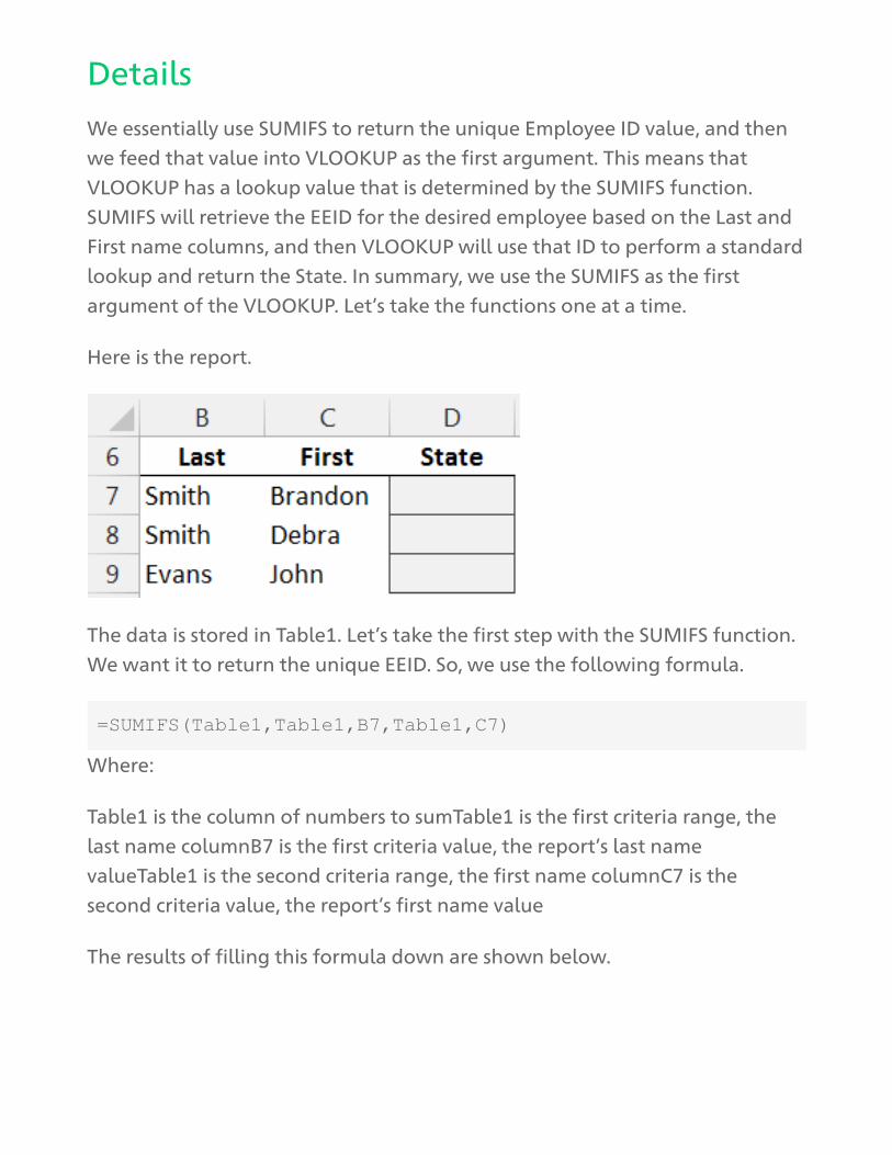
Here is the report.

The data is stored in Table1. Let’s take the first step with the SUMIFS function.

We want it to return the unique EEID. So, we use the following formula.

=SUMIFS(Table1,Table1,B7,Table1,C7)

Where:

Table1 is the column of numbers to sumTable1 is the first criteria range, the

last name columnB7 is the first criteria value, the report’s last name

valueTable1 is the second criteria range, the first name columnC7 is the

second criteria value, the report’s first name value

The results of filling this formula down are shown below.

We were able to use SUMIFS to retrieve the Employee ID based on matching

the First and Last name values. So far so good? Now, we just need to ask

VLOOKUP to return the State based on the Employee ID.

Note: it is important to note that this technique assumes that each EEID valueis unique within the column, and that only one row will satisfy all SUMIFSconditions. If these assumptions are not met, this technique may not work asexpected. If your data table doesn’t have a unique ID column, you canalways add a helper column that numbers the records 1, 2, 3, and so on.

Let’s use the SUMIFS function above in a VLOOKUP, as shown below:

=VLOOKUP(SUMIFS(Table1,Table1,B7,Table1,C7),Table1,5,0)

 Where:  SUMIFS(…) returns the Employee ID for use as the VLOOKUP’s lookup

valueTable1 is the lookup range, the employee table5 is the column that has

the value to return, the State column0 tells Excel we are looking for an exact

matching EEID value

After filling the formula down, our report is complete, as shown below.

We did it…yay!

Note: It is also interesting to note that this technique can be used with datecolumns as well, and if needed, we could use comparison operators tofind values within a range of dates.

Sample Excel file

Take your Excel knowledgeto the next level!

Enroll today!

made with