Lappeenranta-Lahti University of Technology LUTSchool of Engineering ScienceComputational Engineering and Technical PhysicsComputer Vision and Pattern Recognition

Nima Bahmani

VITAL SIGN DETECTION USING SHORT-RANGE MM-WAVEPULSED WAVE RADAR

Master’s Thesis

Examiners: Associate Professor , Dr. Arto KaarnaMPhil. Markku Rouvala

Supervisors: Associate Professor , Dr. Arto KaarnaMPhil. Markku Rouvala

ABSTRACT

Lappeenranta-Lahti University of Technology LUTSchool of Engineering ScienceComputational Engineering and Technical PhysicsComputer Vision and Pattern Recognition

Nima Bahmani

Vital Sign Detection Using Short-Range Mm-Wave Pulsed wave RADAR

Master’s Thesis

2020

45 pages, 15 figures, 3 table, 1 appendices.

Examiners: Associate Professor , Dr. Arto KaarnaMPhil. Markku Rouvala

Keywords: mm-wave RADAR, pulsed wave RADAR, vital sign, signal processing

Proximity sensors have been improving fast during the last decades. Using a radiationsource and examining the reflected signal, it is possible to investigate the surroundingenvironment without contact. The mm-wave RADAR systems demonstrate tremendouspotential compared to the other proximity sensing options, which are based on soundor light waves. In this study, a 60 GHz RADAR system was used for vital sign detec-tion, such as respiration and heartbeat rate. The potential of the system in measuringthrough the materials was investigated in different transmission scenarios. Three differ-ent algorithms were tested for extracting the phase information, and a standard heartbeatrate measurement device compared the accuracy of the results. The proposed algorithmcan scan the area in the RADAR field of view and obtain remarkable features like theheartbeat rate with a median accuracy of 96.22%.

PREFACE

I would like to express my sincere gratitude to my university supervisor, Arto Kaarna, toguide me through my master’s degree. Special thanks to Markku Rouvala, not only for allthe support he has shown me in this research but also, leading me towards the right pathin life. Further thanks to Huawei company for funding this thesis, and my colleague, PasiPylvas, for his generosity and helps. Finally, thanks to my family for their unconditionalsupports.

Helsinki, November 2, 2020

Nima Bahmani

4

CONTENTS

1 INTRODUCTION 81.1 Background . . . . . . . . . . . . . . . . . . . . . . . . . . . . . . . . . 81.2 Objectives and delimitations . . . . . . . . . . . . . . . . . . . . . . . . 91.3 Structure of the thesis . . . . . . . . . . . . . . . . . . . . . . . . . . . . 10

2 RADAR SYSTEM BENEFITS AND APPLICATIONS 112.1 LIDAR, SONAR or short-range RADAR . . . . . . . . . . . . . . . . . 112.2 Continuous wave or pulsed wave RADAR . . . . . . . . . . . . . . . . . 122.3 Applications of RADAR on detection of the presence and vital sign . . . 12

3 RADAR SIGNAL PROCESSING 143.1 RADAR system overview . . . . . . . . . . . . . . . . . . . . . . . . . . 143.2 Pulsed wave RADAR waveform . . . . . . . . . . . . . . . . . . . . . . 143.3 In-phase-quadrature detector . . . . . . . . . . . . . . . . . . . . . . . . 153.4 RADAR raw data . . . . . . . . . . . . . . . . . . . . . . . . . . . . . . 16

4 PROPOSED METHODS 184.1 Vital sign detection methods . . . . . . . . . . . . . . . . . . . . . . . . 184.2 Phase estimation . . . . . . . . . . . . . . . . . . . . . . . . . . . . . . 184.3 Respiration and heartbeat rate detection . . . . . . . . . . . . . . . . . . 21

5 EXPERIMENTS AND RESULTS 235.1 Measuring the primary I-Q signal . . . . . . . . . . . . . . . . . . . . . . 235.2 Description of experiments and experiment setup . . . . . . . . . . . . . 235.3 Extracting phase using proposed methods . . . . . . . . . . . . . . . . . 265.4 Extracting the respiration . . . . . . . . . . . . . . . . . . . . . . . . . . 295.5 Accuracy of the results . . . . . . . . . . . . . . . . . . . . . . . . . . . 31

6 DISCUSSION 376.1 Current study . . . . . . . . . . . . . . . . . . . . . . . . . . . . . . . . 376.2 Future work . . . . . . . . . . . . . . . . . . . . . . . . . . . . . . . . . 38

7 CONCLUSION 40

REFERENCES 41

APPENDICESAppendix 1: Results from the first experiment.

5

LIST OF ABBREVIATIONSCW Continuous WaveDSP Digital Signal ProcessingEEMD Ensemble Empirical Mode DecompositionEMD Empirical Mode DecompositionFFT Fast Fourier TransformGUI Graphical User InterfaceHCI Human Computer InteractionI-Q In-phase-QuadratureLIDAR Laser Imaging Detection And RangingLPF Low Pass FilterMAF Moving Average FilterMIMO Multiple Input Multiple OutputPW Pulsed WavePRF Pulse Repetition FrequencyPRI Pulse Repetition IntervalPW Pulsed WaveRADAR Radio Detection And RangingRCS RADAR Cross-SectionSONAR Sound Navigation And RangingTOF Time Of FlightUWB Ultra Wide-BandWT Wavelet Transform

6

LIST OF SYMBOLS

Normal symbolsA envelope of the transmitted signalA′ envelope of the received signala lower limit of the rangeb upper limit of the rangec speed of lightd range indexdpeak range index with the highest amplitude within a sweepf0 frequencyGr gain of the received antennaGt gain of the transmit antennaI real part of yIQL number of range samplesM number of sweepsN number of samplesPr received powerPt transmitted powerQ imaginary part of yIQR0 range from the RADAR to the targets sweep indexst step lengtht timeTs sampling interval∆T time of flightx RADAR transmitted signaly RADAR received signalyD filtered and downsampled form of demodulated received signalyIQ demodulated received signal yDyM1 computed I-Q data of Method 1yM2 computed I-Q data of Method 2y∗D complex conjugate of yD6 phase of a complex number

7

Greek symbolsαφ high pass filter factorθ phase∆θ phase shiftλ wavelengthσ mean RADAR cross-section of the target

8

1 INTRODUCTION

1.1 Background

During the second world war, radio detection and ranging (RADAR) systems were devel-oped to track the objects and missiles in long-distances. During that time, sound and lightdetection were the two main options for this purpose. The acoustic detectors were devel-oped in the first half of the 20th century. The light detectors had a very narrow field ofview due to its short wavelength, and the acoustic waves did not have enough efficiency.A better perception of the electromagnetic waves affected the technology to invent novelsystems for long-range discovery. RADAR systems were developed and significantly im-pacted the second world war by detecting the airplane and missiles. The concept wassending an electromagnetic wave and taking back the reflection from the target object.The echo signal was analyzed by its features such as amplitude, time of flight (TOF), andphase shift compared with the transmitted signal.

New advancements in both material science and electronics made it possible to designthe RADAR concept in a tiny package compared to the first generations. Although thesmall package means less power and the scanning narrows to short-range detection, theapplications were designed for the mm-wave RADAR chips. The RADAR chips wereimplemented on portable devices such as mobile phones and tablets, which means theenormous potentials of the RADAR systems can be achievable in a pocket-size device.

Exploring the surrounding environment is feasible via active or passive scanners. Themost obvious example for the passive scanner is a camera that collects the light and con-structs an image. The active scanners are like the RADAR concept. The leading vi-able solutions for the active scanning are Laser imaging detection and ranging (LIDAR),sound navigation and ranging (SONAR), and RADAR. In all of these methods, a wave istransmitted, and the reflected wave is investigated for extracting particular features. Thecomparison between these methods are discussed in Chapter 2.1.

Different types of categorizations are defined for RADAR systems. RADAR is classi-fied recording to the RADAR characteristics such as frequency band and antenna type,RADAR functionality, types of the waveform, and other technical characteristics [1].Recording to this study’s application targets, antenna design, and waveform types are theessential features. The antenna design can be divided into multi-receiver channel RADARand single receivers. The waveform type can classify the RADAR into continuous wave

9

(CW) or pulsed wave (PW) RADAR. Each of these methods has benefits and drawbacks,which are specified in Chapter 2.2.

The short-range mm-wave 60 GHz RADAR integrated silicon device solutions have emergedrecently. By frequency range between 57 GHz to 64 GHz, this RADAR system can pro-vide 7 GHz bandwidth, which is an excellent opportunity to define new applications withreasonable accuracy. This specific bandwidth was utilized for different applications. Thetarget applications with the ability for implementation on the mobile device are expressedas follows:

• Presence and occupancy detection such as people counting, people’s actions classi-fication, room automation, and object detection.

• Human-computer interaction (HCI) such as gesture recognition.

• Material detection such as material classification or sense of touch for the robots.

• wearable assistance solution for people with disability or army.

• Vital signs such as heart rate vibration, respiration rate, human body micro-vibration,blood pressure, and glucose level meter.

The RADAR system’s primary healthcare applications are respiration and heartbeat ratedetection, which is feasible due to this sensor’s high sensitivity to the micro-vibrations.The RADAR which is based on the active scanning make it possible to do contactlessmeasurements. Also, the wave can penetrate through the thin non-metallic materials.This sensor’s contactless feature has a unique potential for health monitoring both withinhospitals and houses.

1.2 Objectives and delimitations

This study concentrates on the vital sign detection ability of the mm-wave RADAR sys-tem. The 60 GHz RADAR system of Acconeer company [2] by the Raspberry Pi board [3]is used for data acquisition. This RADAR system has only one transmitter and one re-ceiver for saving more energy and space in portable appliances. The study is limitedto short-range vital sign detection with the standard environment in which the target isstationary. For this purpose, RADAR raw data analysis and signal processing were con-sidered, and the accuracy of the system was tested. The discovered object in the RADAR

10

field of view was divided into two main categories of an alive or non-alive object. For thispurpose, the vital sign recognition algorithm is scanning the area and detecting the chest’slocation. The objectives of the thesis are summarized as follows:

• Setting up the system and data acquisition using RADAR and Raspberry Pi.

• Chest tracking using RADAR data processing.

• Extracting the vital sign information such as respiration, heartbeat rate.

• Using different algorithms for phase unwrapping.

• investigating the potential of the RADAR in case of transmission over differentmaterials.

• Analyzing the accuracy of the results by using a standard measurement device.

1.3 Structure of the thesis

In this thesis, the vital sign detection methods are performed using a 60 GHz RADARdevelopment kit. Chapter 2 is started with comparing RADAR with other alternativessuch as SONAR and LIDAR. In the following, the advantages and disadvantages of bothCW and PW RADAR are discussed. The mm-wave RADAR’s main applications areoverviewed, and the previous works related to vital signs and presence detection are ex-plained. Chapter 3 is discussing the RADAR concept and the raw RADAR signal. Thesignal processing and proposed algorithms for the respiration and heartbeat rate detectionare explained in Chapter 4. Chapter 5 focuses on the practical results, and the estimationswere acquired using the proposed algorithms. Chapter 6 is making the discussion for thecurrent study and the future work and discuss the accuracy of the results. Finally, a shortconclusion is given in Chapter 7.

11

2 RADAR SYSTEM BENEFITS AND APPLICATIONS

2.1 LIDAR, SONAR or short-range RADAR

For short-range proximity, the most critical sensors are ultrasound, LIDAR, and short-range RADAR. All of these sensors are active and sending a wave and take back the echosignal. Ultrasound sensors employ frequencies from the tenths of kHz to MHz, whichdepends on the sensor specification. The lower frequencies of ultrasound were used forproximity sensing and similar applications as this study. The higher frequencies can pen-etrate the body and be used as an imaging system. The LIDAR uses the optical timeof flight, and the mm-wave RADAR has a wide variety of frequency bands, but in thisstudy, the focus is on 60 GHz RADAR systems. It is possible to discuss these sensors’differences by analyzing the available sensors’ specification and the concept behind thespecific frequency range features. The LIDAR system has the lowest wavelength and canobtain the most precise spatial resolution. The maximum detection range of the RADARis higher than the Ultrasound and LIDAR. The mm-wave RADAR’s minimum range de-tection is small, less than half a millimeter, but the ultrasound sensor chips cannot detectan object in the short-range. Because the miniaturized ultrasound chips use the same areafor transmitting and receiving the signal and there has to be a time gap for the ringingafter signal transmission. The ringing of the transmitters leads to higher decay time.

The LIDAR and RADAR sensor has a wide field of view. The RADAR signal can pen-etrate to the non-metal materials. One of the most valuable outcomes of this feature isthe RADAR robustness against environmental factors. On the other hand, ultrasound andLIDAR are more sensitive to the environment. The ultrasound sensors are better in rangeresolution than object speed estimation, and in general, these sensors are the most afford-able method for proximity sensing. The RADAR sensor has a tremendous ability bothin range and frequency domain, allowing sensing small changes. The LIDAR can havebetter object characterization due to better spatial resolution, but the system is non-robustagainst ambient light. It is possible to perform beamforming by designing a multi-receiverchannel. In this case, the receivers have to be located with half of the wavelength distancefrom each other. The ultrasound sensor array occupies a large space, as an example, usinga wavelength of 40 kHz leads to 4.3mm distance between the sensors. For the 60 GHzRADAR system, the receivers are located with a 2.5mm distance. All of these benefits ofRADAR systems represent it as an essential solution for proximity and ranging.

12

2.2 Continuous wave or pulsed wave RADAR

The short-range small mm-wave RADAR can be categorized into two main types, theCW and PW RADAR. The CW RADAR is transmitting a continuous electromagneticwave, and the receiver receives part of the reflections. The comparison of transmitted andreceived signals can address information about the range and movements of the target.This concept was extended to frequency modulated continuous wave (FMCW) RADAR,in which the frequency is changing periodically over time [4]. The PW RADAR is basedon the TOF concept, which detects the time difference between transmission and receiv-ing the echo of the pulsed signal. "Compared to CW RADAR, the main advantage ofPW RADAR is the intrinsic immunity to multi-path reflection" [5]. The FMCW RADARuse a continuous transmission, which leads to continuous power consumption. The PWRADAR has its complexity, which is due to fast time signal detection. The electro-magnetic waves are traveling with the speed of light, leads to a short TOF. The FMCWRADAR has better doppler resolution than PW RADAR, and on the other, the PW’s sep-arate transmitter and receiver do not suffer from the leakage between these elements [4].

2.3 Applications of RADAR on detection of the presence and vitalsign

This section focuses on the presence and vital sign detection application of mm-waveRADAR. Yavari et al. [6] investigated occupancy monitoring by using a 2.405 GHz CWRADAR system. The system detected the heart rate and respiration by filtering the signalin particular frequencies. The measurement was done for different body moves such aswalking or running, although the vital sign was measured in a stable condition. Lurz etal. [7] presented a 24 GHz doppler RADAR system for presence and respiration detec-tion. By using intermittently measuring, the power consumption was significantly reducedcompared to CW RADAR. The measurement was arranged by placing the RADAR sys-tem at a precise distance from the target, and the proposed system was able to detect therespiration. Baird et al. [8] introduced an algorithm for occupancy detection in a roomusing principal component analysis (PCA). The measurement was taken with ultra wide-band (UWB) RADAR in an empty room and a room with one or two persons. The signalenergy can be different in various bins, and the highest energy peaks show a strong echoat a certain distance so that the occupancy detection would be achievable.

Santra et al. [9] proposed a RADAR system for occupancy sensing applications by using

13

a 60 GHz FMCW RADAR sensor. The experiment was done for different human bodymovement classes such as macro doppler (walking and running), micro doppler (workingon a computer), and vital doppler (heartbeat and respiration). The result claimed an abso-lute presence detection, but the vital sign detection was performed in sitting or standingidle case. The vital sign was calculated by interferometric techniques and estimated theheartbeat rate. Santra et al. [10] proposed a multi-channel FMCW RADAR system withtwo receivers and two transmitters, which was able to construct a two-dimensional imagewith a specific field of view. By using multiple-input multiple-output (MIMO), which isan advanced phased array system, the RADAR system can create an image in the hori-zontal plane and can identify the people and objects in a particular field of view. Also,because of the great potential of FMCW RADAR in the frequency domain, the systemwas able to identify the heartbeat rate and respiration individually by using proper filters.

Many studies are explicitly focussing on the noncontact heartbeat rate and respirationdetection [11–14]. Zakrzewski et al. [11] proposed a novel method for heartbeat ratedetection. The robustness of the measurements was evaluated for different angles be-tween the sensor and the human chest. Alizadeh et al. [12] proposed a remote heartbeatrate sensing using a 77 GHz RADAR system. The results were measured by facing theRADAR system by a distance to the target person to simulate sleep monitoring. Hu etal. [13] developed an algorithm for measuring the heart rate variation and respirationusing wavelet transform (WT) and empirical mode decomposition. The algorithm wastested for both the simulated target and the human body. The respiration has an artifactin heartbeat rate detection, but the algorithm was able to separate these two features. Themost common solution is a narrowband filter recording to the target feature, which haslimited ability. Zakrzewski and Vanhala [14] developed an algorithm for dividing thesetwo features utilizing complex-valued Independent Component Analysis.

14

3 RADAR SIGNAL PROCESSING

3.1 RADAR system overview

The electromagnetic wave transmits from the RADAR and hits the target. The transmittedwave characteristics and the target object features can estimate the proportion of the wavereturn to the RADAR system. The time of flight plays a significant rule in signal attenua-tion. Furthermore, the RADAR cross-section (RCS) of the target affects the echo signal.The RCS depends on the size, shape, and material properties of the target. Consequently,the metal objects can be detected from longer distances compared to the object with thesame size by non-metal material properties. The received power is presented as [15]

Pr =PtGtGrλ

2σ

(4π)3R40

(1)

where Pr is the peak received power, Pt is the transmitted power, Gt is the gain of theantenna in the transmitter , Gr is the gain of the antenna in the receiver, λ is the carrierwavelength, σ is the mean RCS of the target and R0 is the range from the RADAR to thetarget.

The active PW RADAR is based on the TOF concept, which measures the electromagneticwave’s travel time between transmission and receiving the signal. The range sample, R0,is calculated as [15]

R0 =c∆T

2(2)

where c is the speed of light, and ∆T is TOF. The ∆T is the period between sendingand receiving the RADAR wave. It is obtainable using matched filters, which applies theconvolution of received wave and time-shifted transmitted wave [16]. The time-shiftingmakes it possible to estimate the range or fast-time samples.

3.2 Pulsed wave RADAR waveform

Modeling of the RADAR waveforms can make a better understanding of the concept. Asummary of the modeling is available in the following text; more expanded derivation isin [15]. The PW RADAR can transmit the pulse with the general form as follows:

x(t) = A(t) cos(2πf0t+ θ) = Re{(A(t) exp (jθ)

)exp (2πjf0t)

}(3)

15

where x is the RADAR transmitted pulse, t is time, A is the Gaussian envelope, A(t) =

exp(−t2/2λ2) [17], θ is the phase, and f0 is the RADAR’s carrier frequency which in thisstudy indicates f0 = 60 GHz. Therefore the amplitude of the cosine signal is changing inaccordance with the Gaussian envelope, and this modulated signal is a pulse wave. Thispulse was expressed as a vector with the amplitude of A and the phase of θ. This wave ishitting the target and travel back to the receiver and is modeled as

y(t) = A′(t) cos

[2πf0

(t− 2R0

c

)+ θ

]

= Re

{A′(t) exp

[j(θ − 4π

λR0

)]exp (2πjf0t)

}(4)

where y is the RADAR received pulse, t is time, A′(t) is the envelope of the receivedsignal, R0 is the range of the target, and λ is the wavelength. The amplitude has changed,and the wave is delayed by ∆T = 2R0/c. Also, the phase of the received pulse is shiftedby ∆θ = −4πR0/λ radians [15]. In Eq. 4, A′(t) is the multiplication of a constantwith the delayed envelope which means, A′(t) = (Constant)×A(t− 2R0/c) [16]. Thisconstant represent the loss of power which is the ratio of Pr and Pt, as it was demonstratedin Eq. 1.

3.3 In-phase-quadrature detector

The pulse in the receiver splits into two channels. The procedure is demonstrated inFig. 1 [15], which combine the signal with reference signals to produce the in-phase(I) channel, and quadrature (Q) channel. Using complex channels makes it possible toestimate the received signal’s amplitude and phase compared to the transmitted signal.The received signal is mixed with two reference oscillators with a 90-degree phase shiftbetween them. The mixed signals were low pass filtered to remove the sum frequencyterm. If there was just one mixer, the total phase and amplitude could not be distinguished.The coherent or in-phase-quadrature (I-Q) detector uses the complex output, and by thisconcept, it is possible to calculate phase and amplitude separately [15].

16

Figure 1. In-phase-quadrature (I-Q) Detector. [15]

3.4 RADAR raw data

The method, which is presented in Fig. 1 is the I-Q demodulation. The RADAR receivedsignal y(t) in Eq. 4, is demodulated to A′(t)exp(jθ) ,and it means the carrier frequencyis excluded [17]. The I-Q demodulated signal has a real part, I , and an imaginary part,Q. The I-Q demodulation is utilized to the received raw data y(t) and produced the I-Qsignal yIQ as

yIQ[s, d] = I[s, d] + jQ[s, d] (5)

where s is the slow time index or sweep number ,and d is fast time index or range index.The real and imaginary part of the yIQ is the I and Q channel output of the I-Q demodula-tor, respectively, which is demonstrated in Fig.1. For each selected range, there is a timeexpectation that can be calculated from Eq. 2, which corresponds to a particular match-ing filter. Therefore, one yIQ is estimated for each range samples, and the estimationsare updated in the time domain, which corresponds to different sweep numbers. The I-Qsignal is represented as Fig. 2 [18]. Each of the blocks in Fig. 2(a) represents a complexnumber for a specific distance to the sensor. The fast time sampling interval is Ts, and Lis the number of range samples in each sweep. This scenario was renewed and producedanother dimension to the data as slow time information. Pulse repetition frequency (PRF)is the numbers of the transmitted signal per second, and the pulse repetition interval (PRI)is the time between sweeps. Fig. 2(b) [18] shows the fast and slow time RADAR data.

In Fig. 2(a), each of the samples corresponds to a particular range. The number of rangesamples depends on the step length, which refers to range resolution and the range scan-ning region. The range samples are modeled as

R0 = a+ d× st, a < R0 < b, (6)

17

where R0 is the range sample, a is the lower limit of the range, b is the upper limit ofthe range, st is the step length ,and d is an index to range samples, 0 < d < L. Forexample, if the range scanning region is between 0.4m to 0.6m, the first range samplecorresponds to 0.4m, and the last range sample belongs to 0.6m. If the step length is0.48mm, it means scanning the radar field of view from 0.4m to 0.6m with the stepsof 0.48mm, such as 400mm, 400.48mm, 400.96, .... After I-Q demodulation, a complexnumber is provided for each of the data samples. One sweep means a set of fast time orrange samples. Fig. 1(b) shows the repeated sweeps which construct the slow time axis.

Figure 2. (a) Fast time samples of one sweep which contains L samples over the range, (b)Fast and slow time for M sweeps. Each of the fast time samples corresponds to a specific range,representing the range information, which is varying in time through the slow time dimension[18].

18

4 PROPOSED METHODS

4.1 Vital sign detection methods

The target can be detected by calculating the I-Q signal’s amplitude in the RADAR fieldof view. Because a reflected signal with high amplitude in a specific range confirmsthe presence of an object in that particular range. In this study, different methods wereapplied for extracting the desired data within each sweep. Each sweep consists of Ldifferent range data and different methods employed to extract a phase information foreach sweep. According to Fig. 2(a), different methods obtain one phase data instead ofthe whole of the fast-time samples in each sweep. For estimating the phase information,the following three methods are described:

• Method 1 is considering the specific range sample with the highest signal amplitude.

• Method 2 is based on averaging the phase information of all of the range samples.

• Method 3 is based on the Acconeer evaluation software and is a reference method[19].

4.2 Phase estimation

Method 1 is adopting the echo signal’s maximum amplitude and estimate the phase ofthat specific range. Recording to the particular use case of this setup, it is consideredthat the range with the highest amplitude is a representative of the human body. In Eq. 6for each sweep number (s), there are L numbers of complex data. Method 1 starts byfinding the maximum amplitude of these complex numbers for each sweep and selectingone complex number with the highest amplitude. Method 1 estimate the I-Q signal as

yM1[s] = yIQ[s, dpeak] = I[s, dpeak] + jQ[s, dpeak] (7)

Where yM1 is the computed I-Q data of Method 1, yIQ is the initial I-Q signal, s is theslow time index or sweep number, dpeak is the range index with the highest amplitudewithin a sweep, and d is the fast time index or range index. Method 1 has the potential todetect multiple objects and extract vital signs from different ranges. Because in Method1, the I-Q data was extracted from the range data with the highest signal amplitude, and

19

it can be extended to find multiple peaks in the range data. In this case, the algorithm canfind, for example, two different peaks that correspond to two different alive people.

Method 2 uses the whole of the I-Q data in each sweep and summing up these complexnumbers for each sweep. Thus, a complex number is computed in each sweep as

yM2[s] =L−1∑d=0

yIQ[s, d] =L−1∑d=0

I[s, d] + j

L−1∑d=0

Q[s, d] (8)

Where yM2 is the computed I-Q data of Method 2, yIQ is the initial I-Q signal, s is theslow time index or sweep number, and d is the fast time index or range number. Method2 is the most simplified algorithm that sums all of the variations in each sweep and isdesigned to show a simplified method’s accuracy, which has the least computation cost.

The I-Q data extracted with Method 1 and Method 2 provide a time series of complexdata samples. For each sweep, phase information was estimated, which meansM numberof phase data. This phase information computed from the I-Q data must be unwrapped,which means the phase information with a sudden significant change must be shifted.Therefore, the unwrapping can remove the sudden changes, and the final phase informa-tion is a smooth signal. The algorithm implemented in unwrap function in Matlab canshift the phase information [20]. The jump threshold value has the default value, whichis π. For calculating the phase information, arctangent demodulation was tested, and theresult was unwrapped, but discontinuity may happen [21]. Thus, estimating the I-Q dataphase and unwrapping the results with Matlab unwrap function can cause some discon-tinuity in the output.

In Method 1 and Method 2, one I-Q data was extracted for each sweep, which meansthe range information is eliminated. It means recording to Eq. 7,8 the I-Q data loses itsrelevance to range and is simply relevant to the sweep index. Thus, the I-Q data for eachsweep is a representative of the whole of the fast time samples. Instead of estimatingphase and applying Matlab unwrap function, phase extraction was determined with adifferent algorithm as [21]

θ[s] =s∑

k=1

I[k]{Q[k]−Q[k − 1]} − {I[k]− I[k − 1]}Q[k]

I[k]2 +Q[k]2, (9)

where θ is the phase for one sweep, k is the sweep number counter, s is the sweep number,I is the real part, and Q is the imaginary part of yM1 or yM2 (depends on which methodwas applying). This method uses the derivative of the arctangent demodulation, and in thecase of online data processing, the phase can be unwrapped sweep by sweep. The chest

20

displacement is obtainable by modifying the phase variation. The chest displacement isrepresenting the changes in range data. The phase information was modified into thedisplacement, using λ = c/f = 4.99654mm. As an example, for 2π phase changes, thedisplacement is calculated by R0 = λ∆θ/4π ≈ 2.5mm.

The Method 3 is starting by downsampling, and next, it is followed by a noise reductionapplying a low pass filter to the time dimension. The next step is phase estimation, whichwas calculated by [19]

θ[s] = αθθ[s− 1] + 6{ L−1∑d=0

yD[s, d]y∗D[s− 1, d]}, (10)

where θ is the phase, yD[s, d] is filtered and downsampled for of yIQ[s, d] , αθ is a highpass filter factor, L is the number of fast time samples, s is sweep index, d is range index,6 is the phase of complex number, and y∗D is the complex conjugate of yD. For eachsweep, one phase data was calculated and was used for further analysis.

After obtaining the phase data for each sweep, the fast Fourier transform (FFT) can extractthe frequency domain information. The typical respiration rate is between 8 to 24 beatsper minute, and the heartbeat rate in rest position can change between 50 to 90 beats perminute [22]. It means the highest rest respiration rate in the frequency domain is 0.4Hz,and the lowest rest heartbeat rate is 0.8Hz. Thus, the harmonics of respiration can overlapwith heartbeat rate frequency [23].

The proposed heartbeat variation algorithm by Hu et al. [13] was based on wavelet trans-form and ensemble empirical mode decomposition (EEMD). The empirical mode decom-position (EMD) uses the signal’s maximum and minimum points to make higher andlower envelopes. The mean value of these envelopes can estimate the signal’s lower fre-quency component, and the high-frequency component can be estimated by subtractingthis mean value from the signal [24]. This procedure is repeating to obtain more com-ponents from the signal. Due to the vulnerability of EMD in the presence of noise, theEEMD was developed. In this method, the intrinsic mode functions were calculated afteradding white noise to the signal [24]. The WT was estimated as a concept obtained byscalable windowing of the Fourier transform [25]. During this procedure, the signal’s highand low-frequency components were extracted by the signal’s long or short windowing.

Computational complexity of different phase estimation methods

The phase estimated by Method 1 and Method 2 requires phase unwrapping to remove the

21

discontinuities, as it was shown in fig. 3. The estimated phase by Method 3 does not havea discontinuity, and phase unwrapping is unnecessary. According to Eq. 10 in Method 3,an angle was estimated for each sweep, which was based on the multiplication betweenyD and y∗D. This angle is representative of the phase variation between two sweeps.Thus the final phase was calculated by summing phase change with the phase, which wascalculated from the previous sweep. Method 1, shown in Eq. 7, is based on finding themaximum signal amplitude in each sweep. Thus the signal amplitude was estimated foreach sweep, and the I-Q value of that specific range sample was considered for the phaseunwrapping. Method 2, , presented in Eq. 8, requires the summation of all of the rangesamples in each sweep. Hence the Method 1 and Method 2 has less computational costcompared with Method 3. According to Matlab’s elapsed time for each method, Method1 has approximately 8% more computational cost than Method 2. Also, Method 3 hasaround 23% higher computational cost than Method 2.

4.3 Respiration and heartbeat rate detection

Fig. 3 shows the proposed setup for heartbeat and respiration detection. The procedurewas started by phase calculation by performing Method 1, Method 2, and Method 3 oncalibrated I-Q signal. The phase data was unwrapped, and by implementing WT, therespiration rate was estimated employing WT’s approximation components. The WT’sdetail components are representative of the heart movements (because it has higher fre-quency), and the approximation is selected as a representative of the respiration (due tothe lower frequency). Three different digital signal processing (DSP) was used to calcu-late the heartbeat rate. The DSP 1 consists of WT, detecting the relevant details, movingaverage filter (MAF) that reconstructs the signal, and peak detection, which finds the peakto calculate the heartbeat rate. The DSP 2 is created by using WT, EEMD, MAF, and peakdetection. DSP 3 is the only DSP that is not based on WT and starts by a bandpass filterfrom 0.7Hz to 2.5Hz. This frequency corresponds to 42beats/min and 150beats/min,respectively. Then the MAF has reconstructed the signal, and peak detection could findthe exact location of the peaks in the time domain. The final heartbeat rate in all DSPswas calculated using the average value of the period between the peaks and converting itinto beats per minute.

22

Figure 3. The proposed setup for vital sign detecion.

23

5 EXPERIMENTS AND RESULTS

5.1 Measuring the primary I-Q signal

The raw data was obtained by transmitting signals and reading the echo signal as in Eq. 4.The final data samples, as demonstrated in Fig.2, contain I-Q data, which has both am-plitude and phase. Each of these data samples is related to one transmitted and receivedpulse. These measurements were optimized by the pulse width and transmitted signalgain. Without considering phase information, the amplitude data can provide a rough es-timation of the region of interest. The I-Q signal can provide better information about theobject’s micro-vibrations and is the data with more sensitivity. The I-Q signal containsthe phase information, and the small changes in the object can have a significant impacton the phase response.

The raw I-Q data is captured based on the algorithms of the Radar software [19]. Becausethe first step is raw data calibration, which was already done in the software algorithm. Itindicates that the I and Q data was calibrated to have a 90-degree phase difference. Hence,The I-Q data in Fig. 3 is the calibrated data.

A Python exploration tool software accompanies the hardware setup with a stable graphicunit interface (GUI) [19]. It is possible to capture the data with several sensors and usethe desired configuration to scan a specific range. Using the exploration tool and settingthe configurations for scanning specific range and particular pulse length, it would bepossible to do the measurements. These measurements were saved, and the data was usedfor further analysis in other software such as Matlab.

5.2 Description of experiments and experiment setup

This study uses the A111 RADAR sensor [2], which is a single channel RADAR; there-fore, it only has one transmitter and one receiver. The Raspberry Pi 4 with the Raspbianoperating system was adopted for capturing the data, and the signal processing part forgenerating the raw I-Q data was done in Python by the producer. The I-Q data weretransferred to Matlab for further analysis.

A mock-up was printed with a 3D printer, and the sensors were placed on the corners ofthe tablet-like device. A radome or RADAR dome is the RADAR protector [26], and in

24

this study, it indicates the front layer on top of the RADAR sensor. The distance betweenthe RADAR chip and the radome and the radome’s thickness also must be optimized. Thepermittivity of the radome is the main factor that affects this optimization task. Besides,it depends on the target application. In this study, the goal is a commercial product inwhich miniaturization plays a significant role. It has to be tested in practice to find thebest optimization solution. Data acquisition was made by using a free space RADARwithout implementing a radome. In this case, the results are not dependent on the radomedesign, and this step can be done in product development.

A person was sitting on a chair in the rest mode, and the sensor was facing the chest withroughly R = 40cm distance. During this research, the robustness against the movementwas not studied, so the data was captured with minimum artifacts. As a reference device,Bittium Faros 180 electrocardiogram [27] was used to capture the heart rate variationsimultaneously.

The data was captured by the RADAR setup in three different RADAR positions. Fig.4 demonstrates the RADAR positions and the general path of the RADAR wave, whichprovides the desired data. The main target application is fixing the RADAR system in afixed position, which is shown in Fig. 4 (Dataset 1). Most of the data set are captured in theRADAR fixed position to make a reasonable judgment about the system’s accuracy in thisconfiguration. The RADAR was fixed on a table, and the distance between RADAR andchest was roughly 50cm. In Fig. 4 (Dataset 2), the RADAR setup was held in hand, andthe RADAR field of view was covered with a wall with roughly 55cm distance. Lastly, inFig. 4 (Dataset 3), the RADAR is mounted on the chest, and it is faced to the outside. Inthis setup, there has to be a fixed position object which covers the RADAR field of view.In this experiment, the RADAR was faced with a wall with an approximate distance of75cm.

Figure 4. Various RADAR positions give different datasets.

25

The dataset features are expressed in Table 1, which shows different RADAR positions,the number of data, and the scanned range for each of the datasets. The scanned rangedescribes the specific ranges which were scanned by RADAR. The step length for all ofthe datasets is 0.48mm, which confirms the range resolution. The step length specifiesthe number of range data in one sweep. Thus, The L in Fig. 2(a) depends on two factors,the scanned range, and step length. The received gain was 0.5, and all of the datasetswere captured by profile number 2 recording to the RADAR software. This profile makesa balance between signal strength and range resolution. The update rate for the whole ofthe experiments was set at 80Hz.

Table 1. The dataset features and different RADAR positions.

Dataset RADAR position Number of Data Scanned range (m)

1 Fixed on a table 32 0.4 - 0.6

2 In hand 7 0.4 - 0.7

3 Mounted on chest 4 0.6 - 1.0

The Dataset 1 consists of four scenarios, which are represented in Table 2 and in Fig. 5.These classes are designed to investigate RADAR’s potential in measuring the vital signsover different materials. . Approximately half of the Dataset 1 was captured for free space,with a naked chest faced to the RADAR. The first transmission scenario was wearingwinter clothes, which was a thick shirt and a winter jacket. The other situation was a glasslayer with a thickness of 4mmwith a 1cm distance from the RADAR surface. Finally, thecombination of the glass layer and winter clothes was applied to form a more complicatedcondition.

Table 2. Different transmission scenarios for Dataset 1.

Dataset Transmission scenario Number of Data

1-1 Free space 18

1-2 With winter clothes 3

1-3 With glass layer 9

1-4 With glass layer and clothes 4

26

Figure 5. Different transmission scenarios for the RADAR fixed position.

5.3 Extracting phase using proposed methods

The data was captured by RADAR, and the measured data was transferred to Matlabsoftware for further analysis. The phase information was extracted using different phaseestimation methods, as shown in Fig. 3. An example of phase data for Dataset 1-1 is illus-trated in Fig. 6, which includes different phase-detection methods. The first 40 seconds ofthe data were captured in the rest position with normal breathing, but after 40 seconds, thebreath was held to demonstrate the heart-related impact individually. The purpose of thissignal representation is to show the displacement ratio between respiration and heart rate.The respiration has approximately 3.5mm displacement, although the heart-related dis-placement is approximately 0.2mm. Although the step length for the measurements was0.48mm, it was possible to detect smaller displacements. The detected displacement isless than step length because the I-Q data and phase-detection were employed, increasingthe detection resolution. After visualizing the whole of the datasets, it was conceivableto observe the confidence of Method 3 comparing with other methods. However, each ofthe methods has a negative and positive side, which are discussed in chapter 6. The phasedata for all of the different transmission scenarios of Dataset 1 are approximately the sameas Fig. 6. It is not possible to discuss the difference between transmission scenarios just

27

by showing the signal shape. Therefore a detailed analysis was done in chapter 5.5.

0 10 20 30 40 50 60

time (s)

-5

0

5

Dis

pla

cem

ent (m

m)

Method 1

With respiration

Without respiration

0 10 20 30 40 50 60

time (s)

-4

-2

0

2

Dis

pla

cem

ent (m

m)

Method 2

With respiration

Without respiration

0 10 20 30 40 50 60

time (s)

-2

0

2

Dis

pla

cem

ent (m

m)

Method 3

With respiration

Without respiration

Sample Dataset 1-1 unwrapped phase data

Figure 6. An example of Dataset 1-1 in which the phase estimation was done using three differentmethods such as Method 1, Method 2, and Method 3. The data was captured for the RADAR fixedposition and the naked chest. The first part of the data (demonstrated in blue color) have bothrespiration and heartbeat rate. The red part of the plot was captured without breathing and wasformed by the heartbeat rate.

The phase data for Dataset 2 by applying different phase estimation methods are demon-strated in Fig. 7. Compared to the signals in Fig. 6, the respiration data is eliminated, andthe displacement is mainly because of heart rate and body mechanical vibrations. Therespiration feature was eliminated because the setup was held in hand. As a consequence,Dataset 2 does not carry reliable information about respiration.

28

0 10 20 30 40 50 60

time (s)

-20

-10

0D

ispla

cem

ent (m

m)

Method 1

0 10 20 30 40 50 60

time (s)

-20

-10

0

Dis

pla

cem

ent (m

m)

Method 2

0 10 20 30 40 50 60

time (s)

-4

-2

0

2

Dis

pla

cem

ent (m

m)

Method 3

Sample Dataset 2 unwrapped phase data

Figure 7. An example of Dataset 2 in which the phase estimation was done using three differentmethods, such as Method 1, Method 2, and Method 3. During data capturing, the RADAR washolden in hand, and it was facing the wall.

Fig. 8 shows an example of Dataset 3 in which the radar was mounted on the chest. Theexperiments of Dataset 3 were conducted similarly to Dataset 1, which means 40 secondsof normal breathing, and after 40 seconds, it was without respiration.

29

0 10 20 30 40 50 60

time (s)

-10

-5

0D

ispla

cem

ent (m

m)

Method 1

With respiration

Without respiration

0 10 20 30 40 50 60

time (s)

-10

-5

0

Dis

pla

cem

ent (m

m)

Method 2

With respiration

Without respiration

0 10 20 30 40 50 60

time (s)

-6

-4

-2

0

2

Dis

pla

cem

ent (m

m)

Method 3

With respiration

Without respiration

Sample Dataset 3 unwrapped phase data

Figure 8. An example of Dataset 3 in which the phase estimation was done using three differentmethods, such as Method 1, Method 2, and Method 3. During capturing the data, the RADAR wasmounted on the chest, and it was faced with the wall. The first part of the data (demonstrated inblue color) have both respiration and heartbeat rate. The red part of the plot was captured withoutbreathing and was formed by the heartbeat rate.

5.4 Extracting the respiration

The target vital signs of this study are respiration and heartbeat rate. The first stage isextracting the respiration from the signal. After testing different wavelet filters, the WTwith the Symlet6 wavelet shape, and six layers of decomposition were used in Matlab.The WT by enforcing the wavelet shape to different time bands of the original signal,extract the signal details. An example of this transform is illustrated in Fig. 9, which isbased on Dataset 1-1. The approximation at level six represents respiration, and the detailsat levels 5 and 6 carry heart rate information. The original signal can be reconstructed bycombining the approximation at level 6 with all the details from levels 1 to 6.

30

0 10 20 30 40 50 60

-2

0

2

0 10 20 30 40 50 60-3-2-101

Approximation at level 6 (reconstructed)

0 10 20 30 40 50 60

-0.2

0

0.2

Detail at level 6 (reconstructed)

0 10 20 30 40 50 60-0.2

0

0.2Detail at level 5 (reconstructed)

0 10 20 30 40 50 60-0.2

0

0.2Detail at level 4 (reconstructed)

0 10 20 30 40 50 60-0.1

0

0.1Detail at level 3 (reconstructed)

0 10 20 30 40 50 60-0.1

0

0.1Detail at level 2 (reconstructed)

0 10 20 30 40 50 60-0.1

0

0.1Detail at level 1 (reconstructed)

time (s)

Dis

pla

cem

ent (m

m)

The wavelet transform of a sample from Dataset 1-1

Figure 9. The WT of a sample data from Dataset 1-1. Symlet 6 wavelet with six layers ofdecomposition, was used to split the phase data.

31

5.5 Accuracy of the results

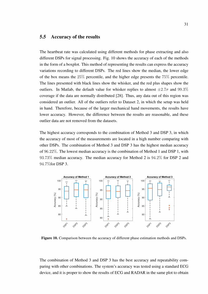
The heartbeat rate was calculated using different methods for phase extracting and alsodifferent DSPs for signal processing. Fig. 10 shows the accuracy of each of the methodsin the form of a boxplot. This method of representing the results can express the accuracyvariations recording to different DSPs. The red lines show the median, the lower edgeof the box means the 25% percentile, and the higher edge presents the 75% percentile.The lines presented with black lines show the whisker, and the red plus shapes show theoutliers. In Matlab, the default value for whisker replies to almost ±2.7σ and 99.3%

coverage if the data are normally distributed [28]. Thus, any data out of this region wasconsidered an outlier. All of the outliers refer to Dataset 2, in which the setup was heldin hand. Therefore, because of the larger mechanical hand movements, the results havelower accuracy. However, the difference between the results are reasonable, and theseoutlier data are not removed from the datasets.

The highest accuracy corresponds to the combination of Method 3 and DSP 3, in whichthe accuracy of most of the measurements are located in a high number comparing withother DSPs. The combination of Method 3 and DSP 3 has the highest median accuracyof 96.22%. The lowest median accuracy is the combination of Method 1 and DSP 1, with93.73% median accuracy. The median accuracy for Method 2 is 94.2% for DSP 2 and94.7%for DSP 3.

DSP1

DSP2

DSP3

80

85

90

95

100

Accura

cy (

%)

Accuracy of Method 1

DSP1

DSP2

DSP3

80

85

90

95

100

Accura

cy (

%)

Accuracy of Method 2

DSP1

DSP2

DSP3

80

85

90

95

100

Accura

cy (

%)

Accuracy of Method 3

Figure 10. Comparison between the accuracy of different phase estimation methods and DSPs.

The combination of Method 3 and DSP 3 has the best accuracy and repeatability com-paring with other combinations. The system’s accuracy was tested using a standard ECGdevice, and it is proper to show the results of ECG and RADAR in the same plot to obtain

32

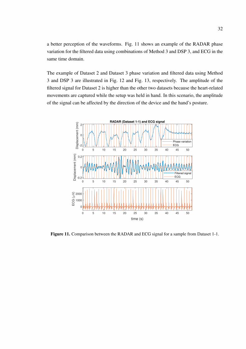
a better perception of the waveforms. Fig. 11 shows an example of the RADAR phasevariation for the filtered data using combinations of Method 3 and DSP 3, and ECG in thesame time domain.

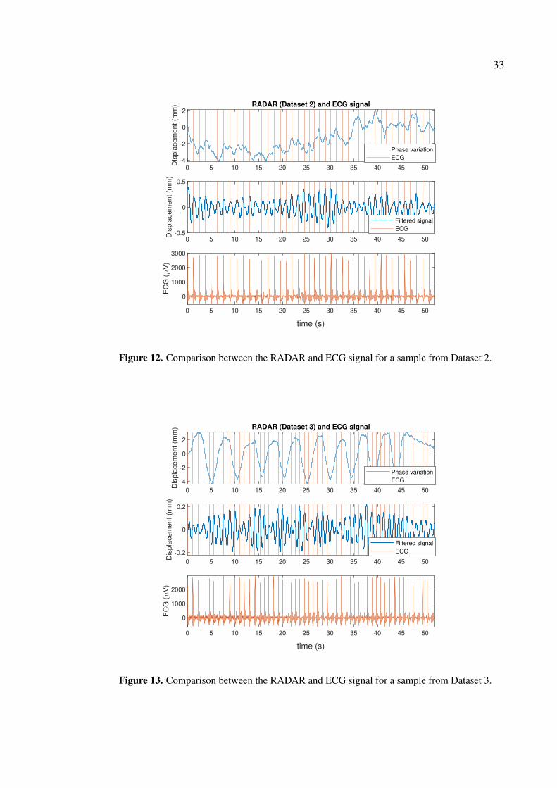
The example of Dataset 2 and Dataset 3 phase variation and filtered data using Method3 and DSP 3 are illustrated in Fig. 12 and Fig. 13, respectively. The amplitude of thefiltered signal for Dataset 2 is higher than the other two datasets because the heart-relatedmovements are captured while the setup was held in hand. In this scenario, the amplitudeof the signal can be affected by the direction of the device and the hand’s posture.

0 5 10 15 20 25 30 35 40 45 50

-2

0

2

Dis

pla

ce

me

nt

(mm

) RADAR (Dataset 1-1) and ECG signal

Phase variation

ECG

0 5 10 15 20 25 30 35 40 45 50

-0.2

0

0.2

Dis

pla

ce

me

nt

(mm

)

Filtered signal

ECG

0 5 10 15 20 25 30 35 40 45 50

0

1000

2000

EC

G (

V)

time (s)

Figure 11. Comparison between the RADAR and ECG signal for a sample from Dataset 1-1.

33

0 5 10 15 20 25 30 35 40 45 50-4

-2

0

2

Dis

pla

ce

me

nt

(mm

) RADAR (Dataset 2) and ECG signal

Phase variation

ECG

0 5 10 15 20 25 30 35 40 45 50-0.5

0

0.5

Dis

pla

ce

me

nt

(mm

)

Filtered signal

ECG

0 5 10 15 20 25 30 35 40 45 50

0

1000

2000

3000

EC

G (

V)

time (s)

Figure 12. Comparison between the RADAR and ECG signal for a sample from Dataset 2.

0 5 10 15 20 25 30 35 40 45 50

-4

-2

0

2

Dis

pla

ce

me

nt

(mm

) RADAR (Dataset 3) and ECG signal

Phase variation

ECG

0 5 10 15 20 25 30 35 40 45 50

-0.2

0

0.2

Dis

pla

ce

me

nt

(mm

)

Filtered signal

ECG

0 5 10 15 20 25 30 35 40 45 50

0

1000

2000

EC

G (

V)

time (s)

Figure 13. Comparison between the RADAR and ECG signal for a sample from Dataset 3.

34

The transmission scenarios and different RADAR locations affect the accuracy of themeasurements, as illustrated in Fig. 14, and the results are presented in Table 3. DifferentRADAR locations are represented in different colors, and the tolerance of the accuracyfor different measurements is demonstrated with the error bars. The calculation was doneusing Method 3 for phase extraction and DSP 3 for the signal processing based on filter-ing.

Method 3 + DSP 3 for different scenarios

Nak

ed C

hest

With

Cloth

es

With

Glass

Lay

er

With

Glass

Lay

er &

Cloth

es

Mou

nted

On

Che

st

Held

by H

and

80

85

90

95

100

Accu

racy (

%)

Dataset 1

Dataset 2

Dataset 3

error bar

Figure 14. Comparison between the accuracy of Method 3 and DSP 3 for different RADARpositions and RADAR transmission scenarios.

35

Table 3. Accuracy of Method 3 and DSP 3 for different RADAR positions and RADAR transmis-sion scenarios.

Dataset Transmission scenario Accuracy (%) Accuracy deviation (%)

1-1 Free space 96.5 5.9

1-2 With winter clothes 95.9 4.6

1-3 With glass layer 96.1 6.9

1-4 With glass layer and clothes 96.3 6.6

2 Held in hand 91.6 16.8

3 Mounted on the chest 93.1 5.1

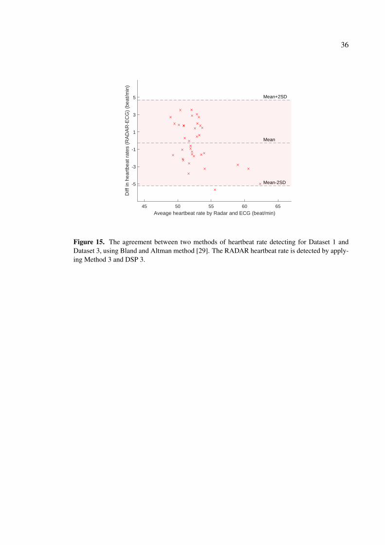
The agreement between two clinical methods can be examined using Bland and Altmanvisualization technique [29]. It is illustrated in Fig. 15, which displays the agreementbetween RADAR heart rate detection and a standard ECG system. The horizontal axisshows the average heartbeat rate by ECG and RADAR system, and the vertical axis repre-sents the difference between the two methods (RADAR-ECG). Three lines labeled in thefigure show the mean value and summation of mean value with standard deviation multi-ply by two. The (Mean+2SD) of the differences is 5.2 beats/min, and (Mean−2SD)

is−4.6 beats/min. The RADAR heartbeat rate results in Fig. 15 are detected by applyingMethod 3 and DSP 3. The Agreement between RADAR and ECG for the whole of themethods and DSPs are illustrated in Appendix 1 in Figs. A1.1, A1.2, A1.3.

36

45 50 55 60 65

Aveage heartbeat rate by Radar and ECG (beat/min)

-5

-3

-1

1

3

5

Diff

in h

eart

beat

rat

es (

RA

DA

R-E

CG

) (b

eat/m

in)

Mean-2SD

Mean+2SD

Mean

Figure 15. The agreement between two methods of heartbeat rate detecting for Dataset 1 andDataset 3, using Bland and Altman method [29]. The RADAR heartbeat rate is detected by apply-ing Method 3 and DSP 3.

37

6 DISCUSSION

6.1 Current study

The vital sign detection was tested with a RADAR sensor, and the algorithm has reason-able accuracy for measuring the respiration, heartbeat rate, and labeling the target as aliveor non-alive. It can find the region of interest with the highest micro-vibration relatedto the human’s vital signs. The respiration was identified with the algorithm based onWT. The size of the chest movements for respiration is roughly ten times greater thanthe heartbeats. Thus, it can affect the heart-related measurement’s accuracy in the pres-ence of respiration. Therefore, the system’s accuracy for measuring the heartbeat rate isimproving when the target holds the breathing.

Different phase extracting methods were used and as it is obvious from Fig. 6, 7, 8, thesignals follow the same patterns. In Method 3, a high pass filter was applied through thecalculation. Consequently, Method 3 does not have a low-frequency shift, which can beseen in Fig. 7. The phase estimated by Method 1 and 2 is shifting roughly 15mm in lessthan 30 seconds, as in Fig. 7, and the reason is the hand displacement. It is not affectingthe accuracy because the corrections were done during each of the DSPs. Phase extractingusing Method 1 and Method 2 is based on arctangent demodulation, and there are minorfluctuations in a few numbers of data samples in which the phase data is not unwrappedprecisely. Although, the output of arctangent demodulation was more satisfying thanunwrapping through the Matlab software. Method 3 has the most stable phase extractionmethod and is suitable for online data analysis.

The results reveal that by combining Method 3 and DSP 3, the highest accuracy wasobtained. This combination has the lowest accuracy variation, with a median accuracy of96.22%. All of the outliers in Fig. 10 are from Dataset 2, which are captured from thehand movements. The lowest median accuracy was for the combination of Method 1 andDSP 1, and the other combinations have greater accuracy. Method 2 has more than 94%

accuracy for all of the possible DSPs, and the results for this method are not affecting bychoosing different DSPs. The difference between the methods is not significant, and it notconceivable to specify the actual difference between these methods in the rest position.

The displacement results for Dataset 2 has more significant variations than the other twomethods. Recording to Fig. 12 the displacements are approximately two times largerthan Dataset 1 and Dataset 3, which means the data is more contaminated with the hand

38

mechanical vibrations. The Dataset 2 signal is not a reliable source for measuring respi-ration, but it carries more information in terms of body micro-vibrations and the level ofstress. The Dataset 1 and Dataset 3 can show the effect of respiration and is more evidentin Fig. 11. After exhaling and pushing out the lung’s air, a few apparent peaks relatedto heart rate can be noticed. It can differ case by case and recording to different bodystructure and respiration patterns, the shape can have a slight deformation. However, thepeaks which are based on the heart rate are more noticeable in lack of respiration.

The transmission scenarios do not significantly affect the accuracy, and the system canmeasure the vital sign over the clothes and a thin layer of glass. Although recording toFig. 14, the error bar is more extended when the glass was added. It means the measure-ments over the thin layer of glass has less accuracy repeatability. The system’s accuracyfor different transmission scenarios varies from 95.9% to 96.5%, which is a tiny dif-ference, and the other errors such as systematic error or respiration style can affect theresults more robust. Dataset 3 has 93.1% accuracy, and although it has less accuracy thanDataset 1, the results are consistent. It is viable to mount the device on the chest andcapture the micro-vibrations, but the mechanical vibrations can also affect the signal’squality. Dataset 2 shows less accuracy, which is 91.6% with a deviation of 16.8%, whichis a considerable number. It means the in hand setup does not have enough accuracy withthe proposed algorithms. The in-hand device can capture extra data regarding mechanicalvibrations, and it has to be removed from the signal.

The agreement between the clinical ECG setup and RADAR based system was demon-strated for Dataset 1 and Dataset 3 in Fig. 15. The upper and lower blue horizontal linesemphasize that if the differences have a Gaussian pattern, 95% of the differences are lyingbetween these two lines [29]. The high and low horizontal dash lines of 5.2 beats/min,and−4.6 beats/minmeans the RADAR heartbeat rate detector may be roughly 5 beats/min

above or 5 beats/min below the clinical ECG system. A clinical device and a commercialproduct do not have the same requirements, and it depends on the target application andthe specific requirements.

6.2 Future work

The phase estimation methods can be extended to capture the presence of multiple targetsand mark those as alive or non-alive. In this scenario, the vital signs can be capturedsimultaneously, and method 1, based on peak detection, can be utilized. By applying thisidea, it would be possible to extract the vital sign of multiple targets in different ranges.

39

This study can be continued by using a sensor with multiple receiver channels. In thiscase, there is a chance to have an angular resolution, and by beamforming, there would bea potential to track two people with the same distance to the RADAR sensor. The othersolution is using a MIMO setup and scan the RADAR field of view to add the angularresolution. Also, an optimized radome can be designed for the actual devices dependingon the end applications.

40

7 CONCLUSION

The ability of the RADAR vital sign detection was studied and implemented by 60GHz

pulsed coherent RADAR system. The algorithm can measure the respiration chest move-ments with excellent accuracy over various materials. The heartbeat rate was calculatedand compared with the clinical reference device. It is possible to calculate the heartbeatrate with fair correctness in case of rest heart rates. Thus, it is a reliable method for sleepmonitoring and tracing the apnea. The RADAR is detecting the respiration and the heart-beat rate over a thick layer of clothes. The heartbeat rate is detectable using the RADARsystem for estimation of the hand mechanical vibrations. The 60GHz RADAR sensorshave the potential to be integrated into wearable silicon device solutions.

41

REFERENCES

[1] B.R. Mahafza. Radar Systems Analysis and Design Using MATLAB Third Edition.Taylor & Francis, 2013.

[2] XC112 connector board and XR112 reference board with one A1 radar sensor.Available: https://www.acconeer.com/products, Accessed: Sept.20, 2020.

[3] BCM2711 Raspberry Pi 4 Model B 2GB - ARM R© Cortex R©-A72 MPU EmbeddedEvaluation Board. Available: https://www.raspberrypi.org/products/raspberry-pi-4-model-b/specifications/, Accessed: Sept.20, 2020.

[4] A. Santra, I. Nasr, and J. Kim. Reinventing radar: The power of 4d sensing. Mi-

crowave Journal, 61(12):22–37, 2018.

[5] X. Chen, W. Rhee, and Z. Wang. Low power sensor design for iot and mobilehealthcare applications. China Communications, 12:42–54, 05 2015.

[6] E. Yavari, H. Jou, V. Lubecke, and O. Boric-Lubecke. Doppler radar sensor foroccupancy monitoring. In 2013 IEEE Topical Conference on Power Amplifiers for

Wireless and Radio Applications, pages 145–147, Texas, USA, January, 2013.

[7] F. Lurz, S. Mann, S. Linz, S. Lindner, F. Barbon, R. Weigel, and A. Koelpin. Alow power 24 ghz radar system for occupancy monitoring. In 2015 IEEE Radio and

Wireless Symposium (RWS), pages 111–113, 2015.

[8] Z. Baird, I. Gunasekara, M. Bolic, and S. Rajan. Principal component analysis-basedoccupancy detection with ultra wideband radar. In 2017 IEEE 60th International

Midwest Symposium on Circuits and Systems (MWSCAS), pages 1573–1576, 2017.

[9] A. Santra, R. V. Ulaganathan, and T. Finke. Short-range millimetric-wave radarsystem for occupancy sensing application. IEEE Sensors Letters, 2(3):1–4, 2018.

[10] A. Santra, R. V. Ulaganathan, T. Finke, A. Baheti, D. Noppeney, J. R. Wolfgang, andS. Trotta. Short-range multi-mode continuous-wave radar for vital sign measurementand imaging. In 2018 IEEE Radar Conference (RadarConf18), pages 0946–0950,Oklahoma City, USA, June, 2018.

[11] M. Zakrzewski, A. Kolinummi, and J. Vanhala. Contactless and unobtrusive mea-surement of heart rate in home environment. In 2006 International Conference of the

IEEE Engineering in Medicine and Biology Society, pages 2060–2063, New York,USA, August, 2006.

42

[12] M. Alizadeh, G. Shaker, and S. Safavi-Naeini. Remote heart rate sensing with mm-wave radar. In 2018 18th International Symposium on Antenna Technology and

Applied Electromagnetics (ANTEM), pages 1–2, Waterloo, Canada, August, 2018.

[13] W. Hu, Z. Zhao, Y. Wang, H. Zhang, and F. Lin. Noncontact accurate measurementof cardiopulmonary activity using a compact quadrature doppler radar sensor. IEEE

Transactions on Biomedical Engineering, 61(3):725–735, 2013.

[14] M. Zakrzewski and J. Vanhala. Separating respiration artifact in microwave dopplerradar heart monitoring by independent component analysis. In SENSORS, 2010

IEEE, pages 1368–1371, 2010.

[15] M.A. Richards, W.A. Holm, and J. Scheer. Principles of Modern Radar: Basic

Principles, Volume 1. Electromagnetics and Radar. Institution of Engineering andTechnology, 2010.

[16] D. Montgomery and G. Holmén. Surface classification with millimeter-wave radarfor constant velocity devices using temporal features and machine learning. Master’sthesis, Lund University, Sweden, 2019.

[17] E. Dagasan. Hand gesture classification using millimeter wave pulsed radar. Mas-ter’s thesis, Lund University, Sweden, 2020.

[18] M.A. Richards. Fundamentals of Radar Signal Processing, Second Edition.McGraw-Hill Education, 2014.

[19] Acconeer python exploration tools, sleep breathing process. Available:https://acconeer-python-exploration.readthedocs.io/en/latest/index.html, Accessed:Sept.20, 2020.

[20] The MathWorks Inc. Available: https://se.mathworks.com/help/matlab/ref/unwrap.html,Accessed: Sept.20, 2020.

[21] J. Wang, X. Wang, L. Chen, J. Huangfu, C. Li, and L. Ran. Noncontact distanceand amplitude-independent vibration measurement based on an extended dacm al-gorithm. IEEE Transactions on Instrumentation and Measurement, 63(1):145–153,2013.

[22] D.L. Gorgas and J.L. McGrath. Vital signs and patient monitoring techniques. Clin-

ical Procedures in Emergency Medicine: 4th ed.,(JR Roberts and JR Hedges, Eds.),

Philadelphia,: Saunders, pages 3–28, 2004.

[23] M. Zakrzewski. Methods for Doppler Radar Monitoring of Physiological Signals.PhD thesis, Tampere University of Technology, Finland, 2015.

43

[24] N.E. Huang and S.S.P. Shen. Hilbert–Huang Transform and Its Applications. WorldScientific, 2nd edition, 2014.

[25] L. Debnath and F.A. Shah. Lecture Notes on Wavelet Transforms. Compact Text-books in Mathematics. Springer International Publishing, 2017.

[26] D.J. Kozakoff. Analysis of radome-enclosed antennas. Artech House, 2010.

[27] Bittium faros 180 sensor, Advanced system for offline and online ECG. Available:https://www.bittium.com/medical/bittium-faros, Accessed: Sept.20, 2020.

[28] The MathWorks Inc. Available: https://se.mathworks.com/help/stats/boxplot.html,Accessed: Sept.20, 2020.

[29] J.M. Bland and D.G. Altman. Statistical methods for assessing agreement betweentwo methods of clinical measurement. International Journal of Nursing Studies,47(8):931 – 936, 2010.

Appendix 1. Results from the first experiment.

46 48 50 52 54 56 58 60 62 64 66 68

-10

-5

0

5

Method 1 & DSP 1 for Dataset 1 & Dataset 3

Mean-2SD

Mean+2SD

Mean

46 48 50 52 54 56 58 60 62 64 66 68

-10

-5

0

5

Method 1 & DSP 2 for Dataset 1 & Dataset 3

Mean-2SD

Mean+2SD

Mean

46 48 50 52 54 56 58 60 62 64 66 68

-5

0

5

10Method 1 & DSP 3 for Dataset 1 & Dataset 3

Mean-2SD

Mean+2SD

Mean

Aveage heartbeat rate by ECG and Radar (beat/min)

Diff

in h

eart

beat

rat

es (

EC

G-R

AD

AR

) (b

eat/m

in)

Figure A1.1. The agreement between two methods of heartbeat rate detecting for Dataset 1 andDataset 3.The RADAR heartbeat rate is detected by applying Method 1 and different DSPs.

46 48 50 52 54 56 58 60 62 64 66 68

-10

-5

0

5

Method 2 & DSP 1 for Dataset 1 & Dataset 3

Mean-2SD

Mean+2SD

Mean

46 48 50 52 54 56 58 60 62 64 66 68

-10

-5

0

5

Method 2 & DSP 2 for Dataset 1 & Dataset 3

Mean-2SD

Mean+2SD

Mean

46 48 50 52 54 56 58 60 62 64 66 68-10

-5

0

5

Method 2 & DSP 3 for Dataset 1 & Dataset 3

Mean-2SD

Mean+2SD

Mean

Aveage heartbeat rate by ECG and Radar (beat/min)

Diff

in h

eart

beat

rat

es (

EC

G-R

AD

AR

) (b

eat/m

in)

Figure A1.2. The agreement between two methods of heartbeat rate detecting for Dataset 1 andDataset 3.The RADAR heartbeat rate is detected by applying Method 2 and different DSPs.

(continues)

Appendix 1. (continued)

46 48 50 52 54 56 58 60 62 64 66 68

-10

-5

0

5

Method 3 & DSP 1 for Dataset 1 & Dataset 3

Mean-2SD

Mean+2SD

Mean

46 48 50 52 54 56 58 60 62 64 66 68

-10

-5

0

5

Method 3 & DSP 2 for Dataset 1 & Dataset 3

Mean-2SD

Mean+2SD

Mean

46 48 50 52 54 56 58 60 62 64 66 68-10

-5

0

5

Method 3 & DSP 3 for Dataset 1 & Dataset 3

Mean-2SD

Mean+2SD

Mean

Aveage heartbeat rate by ECG and Radar (beat/min)

Diff

in h

eart

beat

rat

es (

EC

G-R

AD

AR

) (b

eat/m

in)

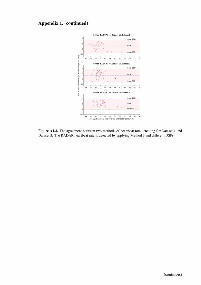
Figure A1.3. The agreement between two methods of heartbeat rate detecting for Dataset 1 andDataset 3. The RADAR heartbeat rate is detected by applying Method 3 and different DSPs.

(continues)