1

Visualizing Misperceptions in Stereoscopic Displays

Robert T. Held1,2 Martin S. Banks1

1University of California, Berkeley 2University of California, San Francisco

Abstract

Stereoscopic displays are becoming more common in fields as diverse as medical imaging and oil exploration. However, to ensure the usefulness of such displays, it is important to minimize any visual misperceptions experienced by their potential users. We present a novel graphical user interface designed for the exploration of misperceptions of stereoscopic images. The software includes controls for stimulus, image acquisition, and viewing parameters. As these settings are adjusted, the user can see their effects on the predicted stereoscopic percept in real time. The software employs two models for stereoscopic distortions to generate these predictions; one based purely on geometry and found throughout the stereocinema literature, and the other based on higher perceptual processes within the visual system. We demonstrate the software’s utility in discovering various types of distortions that arise from improper image acquisition and viewing conditions. We believe this functionality would be useful for engineers who wish to optimize 3D displays for specific viewing situations. We also demonstrate how the software can be used to explore the differences between the two models of stereoscopic misperceptions, and suggest a way to test each model’s accuracy against psychophysical data from human observers. CR Categories and Subject Descriptors: I.3.7 [Computer graphics]: Virtual Reality, I.3.1 [Computer graphics]: Three- Dimensional Displays. Keywords: Depth perception, Virtual Reality, 3D displays, Visualization 1. Introduction

Visual displays such as photographs, video, and animations are essential for communicating ideas and information. Most displays are two-dimensional (2d), but very useful information can be added by three-dimensional (3d), stereoscopic displays. Such displays are now making their way into areas ranging from cinema [1] to medical imaging [2-5]. As the use of stereoscopic displays has spread, the benefits and problems associated with their use have become clearer. One well-documented problem is that the perception of 3d shape and scene layout is often distorted. For instance, standing too close or too far away from a stereoscopic display can alter the perceived size and shape of an object [6, 7]. In some applications, such as cinema, the distortions are not

necessarily a serious problem for the designer [1], but in other applications, such as medical imaging, they can have grave consequences. As a first step to analyzing the sources of stereoscopic distortions, it is important to understand the processes used to produce 3D images.

There are three steps involved in producing a stereoscopic image. (1) The images are acquired by stereo photography or generated by computer graphics. (2) Those images are presented stereoscopically to a human viewer. The presentation requires a way to display the images separately to the two eyes (e.g., red-green color filters, polarizers, or LCD shutter glasses). (3) The images are perceptually interpreted by the visual system.

Misperceptions can arise in a variety of ways in implementing the steps above, but it is useful to distinguish two causes: geometric and perceptual. Geometric misperceptions are caused by inappropriate acquisition-viewing relationships (steps 1 & 2) that result in retinal images that are not the same as those produced by the original scene. Perceptual misperceptions are caused by interpretative processes in the viewer’s visual system (step 3): the retinal images may be geometrically correct, but they are misinterpreted. Keeping with many authors in the current virtual reality and stereocinema literature[1, 6-16], we concentrate on the geometric approach, but later return to the perceptual approach to complete our discussion of stereoscopic misperceptions.

We present an interactive, graphical user interface for exploring the geometric approach to stereoscopic misperceptions. The program allows one to designate stimulus, acquisition, and viewing parameters. It then displays the predicted perceived stimulus in real time. The interactive nature of the visualization allows one to explore how various acquisition and viewing parameters affect one’s percept of a 3D stimulus. It is hoped that the software could therefore be used as a tool for display engineers to design systems that avoid unnecessary stereoscopic misperceptions. We also show how the software facilitated the discovery of some limitations of the geometric approach to misperceptions. We discuss these limitations and possible ways to overcome them with a model more closely matched to the human visual system. 2. Related Work: Geometric Approach Before showcasing the software package mentioned above, it is important to understand the basic concepts on which it was built. We begin with a derivation of the geometric approach to stereoscopic misperceptions. In doing so, we rehash some of the derivations performed by Woods et al. [7], using similar variables and formulas. The derivations allow one to begin with a single point’s 3d coordinates in “real space”, perform a series of transformations, and determine its 3d coordinates as perceived by someone viewing a stereoscopic display. Multiple coordinate systems are necessary for these transformations, and they will be defined as needed.

Step 1: Acquisition (Object space to 2d camera sensors).

2

Figure 2: The cameras’ optical axes can be made to converge by laterally offsetting the sensor relative to the lens. Here, h denotes the amount of sensor-lens offset. Note that in a parallel optical axis setup, h is zero.

Figure 1: Converging cameras capturing a point in 3D space. Variables: po=coordinates of point P, f = camera focal length, t = camera spacing, C =convergence distance of camera optical axes, Vc = angle between cameras’ optical axes, Wc= width of camera sensor, Xcl and Xcr = x-coordinate of P’s projection onto the left and right camera sensors, respectively.

The first step begins with a point, P, in 3d space and determines the 2d coordinates of its projection onto the sensors of a pair of stereoscopic cameras. We begin with a 3d coordinate system, where X is the intercamera axis, Y is the vertical axis positioned at the midpoint between the cameras, and Z is orthogonal to X and Y. P’s 3d X,Y,Z coordinates may be denoted collectively as po. P is projected onto two 2d coordinate systems—one for each camera sensor. Within the sensors, Y is the vertical axis and X is the horizontal axis. P’s coordinates on the left-hand camera’s sensors are denoted by Xcl and Ycl. Likewise, the coordinates on the right-hand camera’s sensors are Xcr and Ycr.

Several settings affect the projection of P onto the sensors. For instance, the cameras’ axes can be setup to be parallel or converging. Both settings have benefits and drawbacks that are beyond the scope of the present discussion [1, 7, 13]. The other relevant parameters for our derivations are f, the focal lengths of the cameras, Wc, the width of the cameras’ sensors, t, the inter-camera separation (between their optical centers), Vc, the angle formed by the camera’s optical axes, and h, the distance between the bisectors of a camera’s sensor and its lens. We define the camera’s optical axis as a ray traveling from the center of its sensor through the center of its lens. Therefore, even if the camera lenses are parallel, if h is nonzero, then their optical axes can be set to converge. Alternatively, h can be set to zero and the lens and sensors can be physically rotated to converge the optical axes. See Figures 1 and 2 for a 2D illustration.

Using the variables listed above with Figures 1 and 2, the following transformations can be derived:

These equations apply for both parallel and converging optical axes. If the cameras’ optical axes are parallel, Vc and h is set to zero. We now have P’s 2D coordinates on the camera sensors. The next step is to present the images on a display. Step 2: Presentation (2d camera sensors to 2d projections). In the presentation step, P’s sensor coordinates (Xcl, Ycl and Xcr, Ycr) must be transformed to 2d picture coordinates (Xsl, Ysl and Xsr, Ysr). The pictures are usually presented on a single display device such as an LCD, CRT, or projection screen. In vision science, stereoscopic images are often presented on two separate displays, one for each eye, on a device known as a haploscope [17]. Here we provide derivations for single-surface displays, since they are far more common. First, the pictures must be magnified to the desired size. The key variable here is Wp, the width of each picture. The simple ratio Wp/Wc provides the magnification from (Xcl, Ycl) and (Xcr, Ycr) to (Xsl, Ysl) and (Xsr, Ysr). Additionally, the left and right eyes’ image may be displaced relative to each other on the surface of the display. The size of the displacement will be denoted d. The combination of the magnification and image offsets produces:

!

Xsl = Xcl

Ws

Wc

"

# $

%

& ' (

d

2

Xsr = Xcr

Ws

Wc

"

# $

%

& ' +

d

2

!

Ysl = YclWs

Wc

"

# $

%

& '

Ysr = YcrWs

Wc

"

# $

%

& '

The 2D coordinates of the disparate points representing P on the display surface are now known.

CCD Sensor

Lens

po

CCD Sensor

Lens

po

!

Xcl = f tan tan"1 t 2 + po (x )

p o (z )

#

$ %

&

' ( "Vc

2

)

* + +

,

- . . "h

Xcr = f tanVc

2" tan"1

t 2 " po (x )

p o (z )

#

$ %

&

' (

)

* + +

,

- . .

+ h

!

Ycl =po (y) f

p o (z )cos(VC

2)+ p o (x )+

t

2

"

# $

%

& ' sin(

VC

2)

Ycr =po (y) f

p o (z )cos(VC

2)( p o (x )(

t

2

"

# $

%

& ' sin(

VC

2)

3

Figure 3: Here, rays are cast from the centers of the eyes and passed through disparate points on the display. The predicted perceived location of P is assigned to the intersection point of the rays. Variables: el and er = 3d coordinates of the left and right eyes, respectively; pl and pr = location of P on the left and right eyes’ images; IPD = interpupillary distance; d = distance between centers of the stereoscopic pictures.

Step 3: Viewing (2d projections to percept). The final step in the geometric approach uses the positions of the disparate points on the screen and the viewer’s eyes to predict the perceived 3D location of P. We will use two new sets of X, Y, and Z-axes. For the first set, we define X and Y as the horizontal and vertical axes on the surface of the display, respectively, while Z is orthogonal to X and Y. The origin is located at the center of the display surface. In this coordinate system the positions of the eyes are denoted by el and er. The eye positions are affected by the viewer’s inter-ocular distance and the translation and rotation of his/her head relative to the display. We also need XYZ coordinates of the disparate points on the display, which we denote pl and pr. Since they lie on the display surface, their Z-coordinates are all zero. Their X and Y-coordinates are given by Xsl, Ysl and Xsr, Ysr. Thus:

!

pl = (Xsl ,Ysl ,0)

!

pr = (Xsr ,Ysr ,0)

Given el, er, pl, and pr, where does the viewer perceive P? To answer this, the geometric approach projects rays that begin in the centers of each eye and pass through the disparate points on the screen. The perceived location of P is assigned to the point of intersection, which we will denote pi (see Figure 3). However, if we use the current coordinate system to determine pi, we will have its coordinates relative to the display, not relative to the viewer. Thus, we want to transform el, er, pl, and pr in the display-centric 3D coordinate system to e’l, e’r, p’l, and p’r in a viewer-centric system. There, X is the interocular axis, Y is the vertical axis positioned midway between the eyes, and Z is orthogonal to X and Y. To begin the transformation, the origin must be placed at the cyclopean eye (the point midway between the eyes, denoted as ec in the screen-centric coordinate system). To accomplish this, ec must be subtracted from el, er, pl, and pr. We then apply the following rotation matrix to make the X-axis coincident with the interocular axis:

!

R(",# ) =

cos(")cos(# ) cos(")sin(# ) $sin(")

$sin(# ) cos(# ) 0

sin(")cos(# ) sin(")sin(# ) cos(")

%

&

' ' '

(

)

* * *

,

where

!

" = # tan#1er (z)# el (z)

er (x)# el (x)

$

% &

'

( ) and

!

" = sin#1 er (y)# el (y)

er # el

$

% & &

'

( ) )

The transformations from screen space to viewer space are thus:

!

" e l = R(#,$ )(el % ec )

!

" e r = R(#,$ )(er % ec )

!

" p l = R(#,$ )(pl % ec )

!

" p r = R(#,$ )(pr % ec )

Now that we are working in a viewer-centric coordinate system, we can find the intersection of the rays originating at e’l and e’r and passing through p’l, and p’r. The intersection can be found using:

!

" e l + ( " p l # " e l )u = " e r + ( " p r # " e r )v

The terms (p’l – e’l)u and (p’r – e’r)v represent the rays leaving the centers of the eyes (e’l and e’r) and passing through the disparate points. The variables u and v are used to indicate a specific point along those rays. When the two sides of the equation are set equal to each other, one can find the point of intersection of the two

rays, assuming it exists. Straightforward mathematical manipulations produce the following solutions to u and v:

!

u =( " e r # " e l )$ ( " p r # " e r )

( " p l # " e l )$ ( " p r # " e r )

!

v =( " e l # " e r )$ ( " p l # " e l )

( " p r # " e r )$ ( " p l # " e l )

We can then determine p’i using

!

" p i = " e l + ( " p l # " e l )u or

!

" p i = " e r + ( " p r # " e r )u

These terms are identical if the intersection exists. Later, the case of non-intersecting rays will be addressed. We now have the perceived location of the original point P in a 3d coordinate system centered on the viewer’s cyclopean eye. Misperceptions can be characterized as discrepancies between p’i and po.

The comparison of p’i and po offers precise measurements of the geometric distortions produced by stereoscopic displays. Additionally, one can use the variables involved in the transformations from po to p’i to qualitatively interpret the optimal viewing conditions. For instance, in stereoscopic presentation, each eye’s image has a center of projection (COP) whose position depends on the camera focal length and orientation of the camera optical axis relative to the film plane. The separation between the COPs depends on the inter-camera separation and image magnification and projector offset. In the geometric approach, two constraints must be satisfied for the predicted 3d percept to match the 3d layout of the original scene. 1) Both of the viewer’s eyes must be positioned at the appropriate COPs [12, 18]. When the eyes are positioned on the COPs, the pattern of light hitting the retinas is the same while viewing the original scene as it is while viewing the stereoscopic pictures. 2) The eye vergence (the angle between the eyes’ optical axes) required to fixate a point in the virtual scene must be the same as the vergence required to fixate the corresponding point in the original scene [12].

We are most interested in what happens when the viewing conditions are not appropriate: specifically, when one or both eyes are not at the appropriate COPs and/or when the eye vergence is not appropriate. Incorrect positioning is commonplace with single-viewer settings and necessarily occurs with multiple viewers. Custom, interactive software was written to explore these conditions and their implications to stereoscopic misperceptions.

pi

el

er

pr

pl

4

Figure 4: Stereo distortion visualization interface. The GUI allows the user to modify stimulus, image acquisition, and viewing parameters independently while viewing the effects on the geometrically predicted perceived stimulus in real-time. The perceived stimulus labeled “Geometric Approach” was implemented in Phase I. In Phase II (discussed later), an alternative, “vertical disparity” approach to stereoscopic misperceptions was added. The numerical values at the bottom of the main window were used for a psychophysical study beyond the scope of this article.

3. Visualization Software (Phase I) Development of the visualization software proceeded in two phases. The first phase involved the creation of the graphical user interface and implementation of the geometric approach to stereoscopic misperceptions. As we discuss later, the program revealed some viewing situations where the geometric approach fails to produce a solution. Phase II of the software development ensued, where alternative approaches to stereoscopic distortions were implemented in an effort to more adequately model the human visual system’s treatment of stereoscopic stimuli.

The program (Figure 4) was comprised of C++, OpenGL, Objective-C, and Cocoa code. The software allowed the user to set stimulus, acquisition, and viewing parameters. Stimulus parameters included the size, position, and orientation of a planar stimulus. Acquisition parameters included camera spacing, focal length, camera orientation (parallel or converging), optical axis convergence distance, convergence angle, and sensor-lens offset. Viewing parameters included image magnification, stereo projector offset, interpupillary distance, and viewer position and orientation (relative to display).

To replicate the predictions of the geometric approach, the software uses the derivations outlined previously. Specifically, the stimulus is represented as three 2D arrays of points. Each array corresponds to the X, Y, or Z coordinate of a point in the stimulus. 2D arrays were chosen to facilitate the display of the stimuli as grids of points (see Figure 4). The arrays of coordinates were fed into the equations derived in the “Related Work” section to determine the position of the points that would appear on a stereoscopic display. These positions were then combined with the 3D coordinates of the eyes to produce pairs of rays whose intersections provided the predicted perceived locations of points within the stimulus (see Figure 3 for a reminder). The software found the intersection point of these rays using the same mathematical approach derived in the previous section.

Once the perceived locations of all the points in the stimulus was found, the software rendered the entire predicted perceived stimulus. It was rendered in teal to allow easy discrimination from the original stimulus, which was rendered in white. On a MacBook Pro with a 2.33 GHz Dual-Core 2 CPU and 2 GB RAM, the mathematical operations necessary to produce the perceived stimulus were completed at a rate that allowed real-time manipulation of the various parameters.

To validate the utility of the software, several viewing positions were investigated, including some that were previously known by the stereocinema community to produce misperceptions. 4. Example Distortions 4.1 Methods To test the visualization software, multiple acquisition and viewing conditions were explored. In each case, a spherical stimulus measuring 20 cm in diameter was simulated 45 cm in front of the stereoscopic cameras. In the proper viewing condition, that is, the situation predicted to produce no stereoscopic misperceptions, the following parameters were used:

Acquisition Parameters: Camera configuration: Parallel Camera spacing: 6.2 cm Camera focal length: 6.5 mm Viewing Parameters: Magnification from CCD image to display: 69.2x Stereo projector offset: 6.2 cm Viewing Distance: 45 cm Interpupillary distance: 6.2 cm Viewer position and orientation: Face parallel with display, midpoint between eyes aligned with center of display.

After the correct viewing situation was setup, we modified several variables independently to observe their effect on the perceived stimulus. The modified variables were: (1) viewing distance, (2) left-right translation of observer parallel to surface of screen, (3) camera spacing, (4) projector spacing, (5) camera orientation, and (6) oblique viewpoint. 4.2 Results

The results of our manipulations are shown in Figure 5. Panel E shows the correct viewing situation, defined using the variables in the Methods section. The images in Figure 5 are screen captures from the software. The viewer is indicated by the pair of eyeballs near the bottom of each panel. The stereocameras, which are sometimes occluded by the eyeballs, are represented by thin blue cylinders. The red vertical lines indicate the cameras’ optical axes. The original stimulus is drawn using white lines. The predicted perceived stimulus is rendered in teal. In panel E, the perceived stimulus is identical to the original stimulus, so only the latter can be seen. Finally, the horizontal green lines represent the simulated display surface. The lines were not visible in the original software, but were added here for clarification. The software does have an option to render the stereoscopic images at the display location, but we have left them out to reduce visual clutter. The images in Figure 5 also include debugging messages near the top. These are irrelevant to our current analysis and can be ignored.

5

Figure 5: Screenshots from the stereoscopic distortion visualization software. Each screenshot shows simultaneous overhead views of the acquisition and viewing setups. Panel D includes labels for the observer, stereocameras, display surface, original stimulus, and perceived stimulus. The vertical red lines indicate the cameras’ optical axes. Panel E shows a correct viewing condition, where the perceived stimulus is identical to the original stimulus. The acquisition and viewing parameters for the correct viewing situation are listed in the Methods section. Panels B and H show the effect of placing the observer further away and closer to the display surface, respectively. Panels D and F show the observer translated to the left and right. Panels A and I show the effect of moving the cameras closer together and further apart, respectively. In panels C and G, the distance between the centers of the left and right eyes’ images, also known as the projector offset, is increase and decreased. The exact values for these modifications can be found in the methods section.

As we step through the various altered acquisition and viewing parameters, there are a few aspects of the perceived stimulus that prove useful in characterizing the stereoscopic misperceptions. These are the distance of the perceived stimulus from the observer, the size of the perceived stimulus, and any change in the shape of the stimulus.

In Figure 5, panels B and H show the result of moving the observer closer and further away from the display, respectively. The observer was placed 22.5 and 90 cm from the display. When the observer is placed closer to the display, the stimulus appears closer to the viewer. Additionally, its spherical shape is compressed in depth. When the viewer is moved farther away

6

Figure 6: Two planes defined using the centers of both eyes and either of the disparate points on the screen. The cross-product of the vectors provides a normal vector that defines the plane.

from the display surface, the stimulus appears further in the distance, with its shape stretched in depth. These results are consistent with those of Woods et al. [7].

For Panels D and F, we translated the observer by 50 cm to the left and right of the optimal viewing position. The translation was performed parallel to the display surface. Here, the most evident distortion is in the stimulus shape. The sphere appears to stretch toward the viewer. This was also predicted by Woods et al. [7].

Panels A and I show the effect of camera spacing on stereoscopic misperceptions. Referring back to the correct viewing situation, in panel E the camera spacing was equal to the interpupillary distance (6.2 cm). In A, the cameras are spaced 3.1 cm apart, and the result is a perceived stimulus that is larger and positioned farther away the view than the original stimulus. When the cameras are spaced 12.4 cm apart (panel I), the stimulus is perceived as smaller and closer than the original. Again, this matches the results of Woods et al [7].

Panels C and G demonstrate the effect of projector spacing. Here, the projectors presenting the left and right eyes’ images on the display are being shifted towards or away from each other. In the correct viewing situation, the centers of the projector’s images are spaced 6.2 cm apart (the interpupillary distance). By changing the spacing of the eyes’ images, we effectively increase or decrease all of the disparities in the image. So in panel C, when the projectors are separated by 7.5 cm, the disparities are increased. The result is a stimulus that is perceived farther away, with a shape that is stretched in depth. Conversely, a projector spacing of 3.1 cm causes the stimulus to be perceived closer to the viewer, with a shape compressed in depth. While Woods et al. do not specifically address these viewing situations, their published derivations lead to the same predictions [7].

The above conditions were effective at demonstrating the utility of the software to explore several causes of stereoscopic image misperceptions. As we have mentioned several times, the predictions produced by the software were identical to those already found by researchers in the stereocinema community. However, when we ran the converging cameras and oblique viewing conditions, the software revealed a crucial flaw in the geometric approach to stereoscopic misperceptions.

When the cameras were set to converge or the observer was set to view the display obliquely, the geometric approach could not provide a mathematical solution to the predicted perceived stimulus. The issue appears to stem from the ray-intersection step. When converging cameras capture stereo images that are then displayed on a single surface, there are several disparate points that lead to skew rays—that is, rays that are not parallel and do not intersect. Obliquely viewing a stereoscopic image generated by either converging or parallel cameras also produces skew rays. In fact, the only rays that seemed to be solvable are those than lie in the visual plane (the X-Z plane, using our last coordinate system). This intriguing result led to an investigation into the conditions necessary to produce skew rays and their effect on human depth perception.

5. Analysis of Skew Rays

To fully address the topic of skew rays, we begin by using our

derivations in the Related Work section to prove their existence under certain viewing conditions. We follow this with a more general way of understanding skew rays using the geometric properties of the viewing environment. Ultimately we show that vertical disparities are the cause of skew rays, and we show how the current stereoscopic literature has dealt with them, as well as how the visual system is believed to use them to form 3D percepts.

5.1 Mathematical Analysis The problem at hand is the lack of intersecting points for the rays that emanate from the centers of the eyes and pass through the disparate points on a stereoscopic display. As a reminder, the intersection points represent where the viewer is expected to perceive a given set of 3D points when they are presented on a stereoscopic display. So if the rays are skew, the geometric approach cannot technically predict what the viewer will see the 3D points. We return to our previously derived equations for these rays to prove that some image acquisition and viewing conditions produce skew rays. Remember that, for a given 3D point in a stereo image, the terms (p’l – e’l)u and (p’r – e’r)v represent the rays, where p’l and p’r are the positions of the left and right eyes’ disparate points, respectively, and e’l and e’r represent the left and and right eyes. These points are all represented in the viewer-centered coordinate system defined earlier. In order for two rays to intersect, it can be shown that the rays must not be parallel and must lie in the same 3D plane. Thus, proof of an intersection (or no intersection) for two rays can be accomplished by determining if the two rays lie in the same 3D plane. We accomplish this by finding the planes defined by the two eyes and the left disparate point, and then the plane define by the two eyes and the right disparate point (Figure 6). We then determine if these two planes are coincident. If they are coincident, then the rays will intersect, assuming they are not parallel.

To define the planes, we use cross-products. The first plane is defined by the cross product between two vectors that originate at the left eye and extend to the left disparate point (vl1) and to the right eye (vl2) (Figure 6). The second plane is defined as the cross product between the vectors originating at the left eye and extending to the right disparate point (vr1) and to the right eye (vr2).

As stated earlier, we want to know the viewing conditions that

produce skew rays. In order to do so, it would be helpful for our analysis to include terms for the translation and rotation of the viewer. This can be accomplished by replacing p’l and p’r with:

!

" p l = R(#,$ )(pl % ec )

!

" p r = R(#,$ )(pr % ec )

Now we can account for the position of the disparate points on the screen, as well as the position of the viewer relative to the screen. Also for simplicity it is useful to refer to the interpupillary

!

vl1 = " p l # " e l

vl 2 = " e r # " e l

vr1 = " p r # " e l

vr2 = " e r # " e l

7

distance as I. Then vl2 and vr2 can both be expressed as (I, 0, 0). Combing the equations above, multiplying out the elements of R(β,γ), and taking into account the fact that pl(z) and pr(z) are both zero (see Related Work) produces the following equations for the cross-products:

We now have a representation for the two planes. Both of the cross-products are defined using a surface normal originating at e’l. However, before we test if the two cross-product are equal, we need to account for the fact that these planes can be coincident but have normal vectors with different magnitudes. We can correct for this by normalizing the vectors and dividing them by the magnitudes |vl1 × vl2| and |vr1 × vr2|. Next, to determine if the planes are coincident, we check to see if their j and k terms are equal to each other (there are no i terms in the equations above). The j terms are:

and the k terms are:

We now have two equalities that can be used as tests for intersecting rays. If the equalities are valid, then the rays will intersect, again assuming that they are not parallel. If they are not valid, then we have found a situation with skew rays and therefore no solution to the geometric approach. We now explore four acquisition and viewing situations. Condition 1: No Observer Rotation In the first viewing condition, the viewer’s face is parallel to the display surface. Additionally, the interocular axis is parallel to the y = 0 line on the display surface. The position of the viewer can be translated in any direction relative to the display. In this condition, the variables β and γ in the rotation matrix R(β,γ) are set to 0. As a result, our dual equalities can be rewritten as:

Examining the equations above, it is clear that the two equalities are only valid if the y-coordinates of the disparate points on the screen are equal. This is always the case when the images are captured using parallel cameras or cameras whose optical axes are set to converge by offsetting the image sensor from the lens. We can therefore conclude that under those capture conditions, when the viewer’s face is not rotated relative to the display, there will be intersections for all of the ray pairs and the geometric approach will provide a solution. Condition 2: Observer Rotation in X-Z Plane Here we begin with the same viewing orientation as in Condition 1, and then rotate (or “yaw”) the viewer in the X-Z plane. Thus, γ is still zero, but now β is nonzero. Our equalities then become:

In this case, the only situation in which the equalities are valid is when pl(y) and pr(y) are equal to ec(y). Simply put, that means that for oblique viewing, only points with no disparity, or disparate points that are located in the visual (X-Z) plane, will produce rays that intersect. All pairs of points with non-zero disparity above and below the X-Z plane will produce skew rays. This explains why the first verion of our visualization software failed to produce solutions under such conditions. Condition 3: Observer Rotation in X-Y Plane This viewing situation is similar to condition 2, except now the viewer’s head is rotated (or “rolled”) in the X-Y plane. Now, γ is nonzero, and β is zero. This results in:

This appears to be the most restricted case. Looking closely at these terms, it becomes evident that the equalities are only valid if

!

vl1 " vl 2 = j (I (sin(#)cos($ )(pl (x)% ec (x)) +

sin(#)sin($ )(pl (y)% ec (y))+ cos(#)(%ec (z))))

+k(I (sin($ )(pl (x)% ec (x)) + cos($ )(pl (y)% ec (y))))

vr1 " vr2 = j (I (sin(#)cos($ )(pr (x)% ec (x))

+sin(#)sin($ )(pr (y)% ec (y))+ cos(#)(%ec (z))))

+k(I (sin($ )(pr (x)% ec (x)) + cos($ )(pr (y)% ec (y))))

!

(sin(")cos(# )(pl (x)$ ec (x))

+sin(")sin(# )(pl (y)$ ec (y))+ cos(")($ec (z)))

=v1r % v2r

v1l % v2l(sin(")cos(# )(pr (x)$ ec (x))

+sin(")sin(# )(pr (y)$ ec (y))+ cos(")($ec (z)))

!

(sin(" )(pl (x)# ec (x)) + cos(" )(pl (y)# ec (y)))

=v1r $ v2r

v1l $ v2l(sin(" )(pr (x)# ec (x)) + cos(" )(pr (y)# ec (y)))

!

"ec (z) =v1r # v2r

v1l # v2l

("ec (z))),

pl (y)" ec (y) =v1r # v2r

v1l # v2l

(pr (y)" ec (y))

where v1r # v2r

v1l # v2l

=j (I ("ec (z)) + k(I (pl (y)" ec (y)))

j (I ("ec (z)) + k(I (pr (y)" ec (y)))

!

sin(")(pl (x)# ec (x)) + cos(")(#ec (z)) =

v1r $ v2r

v1l $ v2l

(sin(")(pr (x)# ec (x)) + cos(")(#ec (z)))

pl (y)# ec (y) =v1r $ v2r

v1l $ v2l

(pr (y)# ec (y)),

where v1l $ v2l

v1r $ v2r

=j (I (sin(")(pl (x)# ec (x)) + cos(")(#ec (z)))) + k(I (pl (y)# ec (y))

j (I (sin(")(pr (x)# ec (x)) + cos(")(#ec (z)))) + k(I (pr (y)# ec (y))

!

"ec (z) =v1r # v2r

v1l # v2l

("ec (z))

(sin($ )(pl (x)" ec (x)) + cos($ )(pl (y)" ec (y)))

=v1r # v2r

v1l # v2l

(sin($ )(pr (x)" ec (x)) + cos($ )(pr (y)" ec (y))),

where v1l # v2l

v1r # v2r

=j ("ec (z)) + k((sin($ )(pl (x)" ec (x)) + cos($ )(pl (y)" ec (y))))

j ("ec (z)) + k((sin($ )(pr (x)" ec (x)) + cos($ )(pr (y)" ec (y))))

8

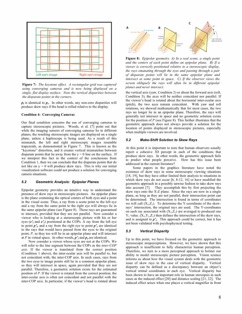
Figure 7: The keystone effect. A rectangular grid was captured using converging cameras and is now being displayed on a single, flat display surface. Note the vertical disparities between the disparate points in the corners.

Figure 8: Epipolar geometry. A) In a real scene, a single point and the centers of each point define an epipolar plane. B) If a viewer is correctly positioned relative to a stereoscopic display, the rays emanating through the eyes and passing through a pair of disparate points will lie in the same epipolar plane and intersect at some point in space. C) If the observer views the screen obliquely the rays will often lie in different epipolar planes and never intersect.

pl is identical to pr. In other words, any non-zero disparities will produce skew rays if the head is rolled relative to the display. Condition 4: Converging Cameras

Our final condition concerns the use of converging cameras to capture stereoscopic pictures. Woods, et al. [7] point out that while the imaging sensors of converging cameras lie in different planes, the resulting stereoscopic images are displayed on a single plane, unless a haploscope is being used. As a result of this mismatch, the left and right stereoscopic images resemble trapezoids, as demonstrated in Figure 7. This is known as the “keystone” distortion, and it creates vertical mismatches between disparate points that lie away from the y = 0 line on the surface. If we interpret this fact in the context of the conclusions from Condition 1, then we can conclude that the disparate points that do not like on y = 0 will produce skew rays. This is why our initial visualization software could not produce a solution for converging camera situations. 5.2 Geometric Analysis: Epipolar Planes Epipolar geometry provides an intuitive way to understand the presence of skew rays in stereoscopic pictures. An epipolar plane is the plane containing the optical centers of both eyes and a point in the visual scene. Thus, a ray from a scene point to the left eye and a ray from the same point to the right eye will always lie in the same epipolar plane (see Figure 8). Those rays are guaranteed to intersect, provided that they are not parallel. Now consider a viewer who is looking at a stereoscopic picture with his or her eyes (e’l and e’r) positioned at the COPs. A ray from the left eye to point p’l, and a ray from the right eye to point p’r are identical to the rays that would have passed from the eyes to the original point, P, so they too will lie in an epipolar plane and will intersect at P in virtual space. In other words, p’i and po are identical.

Now consider a viewer whose eyes are not at the COPs. We will refer to the line segment between the COPs as the inter-COP axis. If the viewer is translated from the correct position (Condition 1 above), the inter-ocular axis will be parallel to, but not coincident with, the inter-COP axis. In such cases, rays from the two eyes to image points still lie in a common epipolar plane, so they will intersect in space, again provided that they are not parallel. Therefore, a geometric solution exists for the estimated position of P. If the viewer is rotated from the correct position, the inter-ocular axis is often not coincident and not parallel with the inter-COP axis. In particular, if the viewer’s head is rotated about

the vertical axis (yaw, Condition 2) or about the forward axis (roll, Condition 3), the axes will be neither coincident nor parallel. If the viewer’s head is rotated about the horizontal inter-ocular axis (pitch), the two axes remain coincident. With yaw and roll rotations, we showed mathematically that for most cases, the two rays no longer lie in an epipolar plane. Therefore, the rays will generally not intersect in space and no geometric solution exists for the position of P (see Figure 8). This further illustrates that the geometric approach does not always provide a solution for the location of points displayed in stereoscopic pictures, especially when multiple viewers are involved. 5.2 Make-Shift Solution to Skew Rays At this point it is important to note that human observers usually report a cohesive 3D percept in each of the conditions that produce skew rays. In other words, the geometric approach fails to predict what people perceive. How has this issue been addressed in the current literature?

Some papers in the graphics literature have noted the existence of skew rays in some stereoscopic viewing situations [18, 19], but they have either limited their analysis to situations in which skew rays do not occur [6, 8-12, 16] or have modified the geometric approach in a possibly unwise fashion to take skew rays into account [7]. They accomplish this by first projecting the skew rays onto the X-Z plane. Since the rays are now in a single plane, as long as they are not parallel, their intersection point can be determined. The intersection is found in terms of coordinates we will call (X1,Z1). To determine the Y-coordinate of the skew-rays’ intersection, the original rays are used. The Y-coordinates on each ray associated with (X1,Z1) are averaged to produced one Y1 value. (X1,Y1,Z1) then defines the intersection of the skew rays, and is assigned to p’i. This approach could be correct, but it has not been validated with psychophysical testing. 5.3 Vertical Disparity Up to this point, we have focused on the geometric approach to stereoscopic misperceptions. However, we have shown that this approach is insufficient to fully characterize human perception. Therefore, we turn to a more perceptual approach to bolster our ability to model stereoscopic picture perception. Vision science informs us about how the visual system deals with the geometric issue of skew rays in the case of vertical disparity. Vertical disparity can be defined as a discrepancy between an object’s vertical retinal coordinates in each eye. Vertical disparity has been shown to have an important role in human stereopsis in such cases as the induced effect [20] and distance scaling [21, 22]. The induced effect arises when one places a vertical magnifier in front

9

Figure 9: Conventions used by Backus et al. (1999). A) The slant of a surface is defined relative to the cyclopean line of sight. The variables µ and γ represent the vergence and version of the eyes. S is the slant of the surfaceSee the text for definitions of HSR and VSR.

of one eye. The magnification of one eye’s image disrupts the light field entering that eye, thereby producing skew rays similar to those that arose in our discussion of the geometric approach. As a result of how the visual system interprets the disparate images (including the skew rays), frontoparallel surfaces appear slanted relative to the viewer’s face. Previously, Backus, et al. investigated how the visual system estimates surface slant in an effort to elucidate the perceptual basis of the induced effect [17]. Two slant estimators were examined. The first slant estimator was based on version, vergence, and the horizontal size ratio (HSR) of a patch on a surface. The HSR is defined as “the ratio of the horizontal angles [a] patch subtends in the left and right eyes, respectively” [17]. The equation for the first estimator follows:

!

S " # tan#11

µln(HSR)# tan($ )

%

& '

(

) * Estimate 1

where µ is vergence (the angle between the eyes’ optical axes) and γ is version (where the eyes are directed azimuthally, see Figure 9). The current geometric approach to stereoscopic distortions predicts perceived slants that are virtually identical to those produced by Est. 1. Therefore, Est. 1 supports the method currently used by the geometric model to assign intersection points to skew lines. The second estimator used vergence, HSR, and the vertical size ratio (VSR), which is the vertical analog to the HSR for a patch on a surface. The equation for this estimator was:

!

S " # tan#1 1

ƒ µ lnHSR

VSR

$

% &

'

( )

$

% &

'

( ) Estimate 2

Backus et al. found that the combination of the estimates provided by Est. 1, Est. 2, and perspective slant cues form a robust estimator for surface slant [17]. They investigated the perceived slants of surfaces when version and VSR were placed in conflict and perspective cues were uninformative. This situation arises in the induced effect. Due to the conflict, Est. 1 and Est. 2 estimated different slants. It was found that Est. 2 more closely predicted the perceived slant when the stimulus was tall, but when the stimulus was short, Est. 1 prevailed. Here we should note that taller stimuli produce vertical disparities (and skew rays) that are more easily measured by the visual system. The interpretation was that VSR was used to estimate slant when it was available, but if it was rendered uninformative, the visual system resorted to an estimate based on version, vergence, and HSR. We can extend this analysis to the case of stereoscopic misperceptions and suggest that a VSR-based interpretation may be weighted more heavily in the presence of skew rays. This is important, because it may mean that the visual system relies on a VSR-based estimate to produce a 3D percept where the geometric approach fails. We will henceforth refer to the VSR-based interpretation as the “vertical disparity approach.” 6. Visualization Software (Phase II) After we discovered that there were multiple ways to predict human perception of stereoscopic pictures, the next logical step was to include the alternatives in our visualization code.

As a first step, we modified the geometric predictions to include Woods et al.’s solution to skew rays [7]. This ensured that any acquisition and viewing parameters would result in a predicted perceived stimulus that was in line with the current graphics literature. Also, we added a warning box to the software to alert the user if any skew rays were present in the stimulus. Finally, the lines and points comprising the perceived stimulus were colored to reflect the level of skewness of the rays at that

location. This was done by increasing the red component of the line or point in very rough proportion to the minimum distance between the skew rays. The coloring scheme can be seen in Figure 4.

The other important addition to the program was the inclusion of predictions based on the vertical disparity approach. The algorithm can be explained in the context of slant perception, as described by Backus, et al. [17]. In the case of slant perception, the concept is that the viewer perceives a slant that is consistent with the vertical disparities incident on the retinas, regardless of the position of the eyes. For instance, consider a stimulus that produces vertical disparities that are consistent with a surface that is centered 30° to the left of the head’s median plane with a slant of 20°. No matter where the stimulus is displayed relative to the head’s median plane, the viewer will perceive the slant as 20°, according to the vertical disparity approach [17]. That is, the stimulus could be presented at 0°, 15°, or 45° to the left or right of the head’s median plane, and as long as it delivers the same vertical disparity patterns to the retinas, its perceived surface slant will not change. This observation facilitated the software implementation of the vertical disparity approach. To predict what the viewer would perceive, the same acquisition and presentation steps were used from the geometric approach. Then, the disparate points were projected from the screen and “burned” onto the back of the retinas. The two eyes were subsequently rotated about their vertical axes to varying degrees and the intersections of the rays projecting from the disparate points on retinal images and passing through the centers of the eyes were found. This was acceptable because, again, the vertical disparity model is only concerned with the pattern of points on the retinas—not the physical orientation of the eyes. If two rays were

10

Figure 10: Screenshot from visualization software showcasing different predictions from the geometric and vertical disparity approaches to stereoscopic perception. The slants of the two predicted surfaces are noticeably different. Also note the red coloring near the top and bottom of the geometric prediction, which indicates the skew rays in this viewing situation.

skew, the solution to their intersection was assigned to the point in space that, when projected onto the retinas, lay the closest to both the disparate points. The root mean square (RMS) error between these assigned points and the original, disparate retinal points were used in a global minimization search to find the rotation of the eyes that provided intersections for all the rays. In reality, rounding errors could sometimes prevent a solution without any skew rays. As a result, our implementation searched for the minimum achievable RMS error and settled on those rotation settings for the eyes. The set of intersections were then used to determine the perceived stimulus. Since this process took a significant amount of time (~ 5 seconds), it was not performed in real time. Rather, the user was required to press a button to update the vertical disparity predictions. Then, as the program searched for the minimum RMS error, it continually updated a rendering of its current guess for the perceived stimulus. This allowed the user to observe the software’s progress towards its final prediction, which is seen in yellow in Figure 10. Our informal tests showed that this minimization search provided predicted slants that were very close to the estimates provided by Backus et al [17]. 7. Model Comparison Once the additional modeling capabilities were added to the visualization software, differences between the predictions of the geometric approach and the vertical disparity approach were explored.

During this brief survey, we used similar conditions to those in Section 4.1. However, we used a planar stimulus that was located approximately 60 cm from the stereocameras. We measured the slant of the surface predicted by our implementation of the vertical disparity model and compared it to the calculations of Backus, et al. [17]. As stated above, the software closely matched their results. Interestingly, we found that the geometric and vertical disparities produced identical predictions when there were no skew rays. However, in conditions with skew rays, such as oblique viewing, the two approaches produced very different predictions, as seen in Figure 10.

The ability of the software to present both predictions was certainly desirable, but it did not provide any indication of what a human observer would actually perceive. We envision a future version of the software that optimally combines the two predictions based on empirical data derived from psychophysical experiments. 8. Discussion / Potential Impact We have presented a novel graphical user interface designed for the exploration of misperceptions of stereoscopic images. The software allows the user to change stimulus, image acquisition, and viewing parameters and witness the effect on the expected stereoscopic percept. The first implementation was based purely on the geometric approach to stereoscopic misperceptions, which is found throughout the stereoscopic cinema and VR literature. This was useful for investigating several viewing conditions, including improper viewing distance, translation of the observer relative to the display, and incorrect projector and stereocamera offsets. As shown in Figure 5, these parameters led to various types of distortions, such as improper perceived stimulus size and shape. One can imagine viewing situations where the distortions are combinations of those seen in Figure 5. This is where the visualization software would be especially useful. Instead of relying on complex mathematical equations to characterize the expected misperceptions, one could enter a set of parameters into the program and see in real-time how a sample stimulus is

distorted. We expect this to be especially useful to display engineers who wish to minimize misperceptions. They could ideally enter their concept design for a display into the program, and then tweak the various parameters in an effort to reduce the distortions perceived by various audiences.

Scientifically speaking, the software led us to realize a critical shortcoming of the geometric approach to stereoscopic misperceptions. Whenever an acquisition and viewing situation produces skew rays (discussed in detail above), the geometric approach fails to produce a solution. This led us to investigate other ways the human visual system processes stereoscopic pictures. The end result was the inclusion of an alternative model that utilizes the pattern of vertical disparities across a stereoscopic picture to form a 3D percept. The final version of the software was therefore able to explore misperceptions predicted by two different models. We are not aware of any other visualization software with this functionality. 9. Future Work

We have mentioned that a key strength of our software is its incorporation of both the geometric and vertical disparity approaches to stereoscopic misperceptions. The next step will be to run psychophysical experiments to determine which approach more closely approximates the human visual system. We will use the software to find viewing conditions that produce different predictions from the two approaches. Those conditions will then be replicated in a psychophysical experiment. An ideal experiment would utilize planar stimuli, with the human observer reporting the perceived slant in a manner similar to Backus et al. [17]. Once the data is collected an analyzed, we intend to

11

incorporate it into our software to produce an optimal model of human perception of stereoscopic displays.

Finally, the ultimate test of the software will be its usefulness according to display engineers. We would like to share our work with researchers and designers in the stereocinema and VR fields and get their feedback on its strengths and weaknesses. This should help us refine the software and meet the needs of its potential users.

References 1. Lipton, L., Foundations of the stereoscopic cinema: a

study in depth. 1982: Van Nostrand Reinhold. 2. Chan, H.P., et al., ROC study of the effect of

stereoscopic imaging on assessment of breast lesions. Med Phys, 2005. 32(4): p. 1001-9.

3. Hu, Y., The role of three-dimensional visualization in surgical planning of treating lung cancer. Conf Proc IEEE Eng Med Biol Soc, 2005. 1: p. 646-9.

4. Peters, T., et al., Three-dimensional multimodal image-guidance for neurosurgery. Medical Imaging, IEEE Transactions on, 1996. 15(2): p. 121-128.

5. Sollenberger, R.L. and P. Milgram, Effects of stereoscopic and rotational displays in a three-dimensional path-tracing task. Hum Factors, 1993. 35(3): p. 483-99.

6. Masaoka, K., et al., Spatial distortion prediction system for stereoscopic images. Journal of Electronic Imaging, 2006. 15(1): p. 13002-13002.

7. Woods, A.J., T. Docherty, and R. Koch, Image distortions in stereoscopic video systems. Proc. SPIE, 1993. 1915: p. 36-47.

8. Diner, D.B., A new definition of orthostereopsis for 3D television. Systems, Man, and Cybernetics, 1991.'Decision Aiding for Complex Systems, Conference Proceedings., 1991 IEEE International Conference on, 1991: p. 1053-1058.

9. Jones, G., et al., Controlling perceived depth in stereoscopic images. Stereoscopic Displays and Virtual Reality Systems VIII, Proceedings of SPIE.

10. Kusaka, H., Apparent Depth and Size of Stereoscopically: Viewed Images. 1991: NHK Science and Technical Research Laboratories.

11. Kutka, R., Reconstruction of correct 3-D perception on screens viewed atdifferent distances. Communications, IEEE Transactions on, 1994. 42(1): p. 29-33.

12. Leiser, D., Y. Bereby, and A. Melkman, Minimizing distortions: seating requirements for stereo projection rooms. Ergonomics, 1995. 38(6): p. 1231-1238.

13. Son, J.Y., et al., Distortion analysis in stereoscopic images. Optical Engineering, 2002. 41: p. 680.

14. Wartell, Z., L.F. Hodges, and W. Ribarsky, Balancing fusion, image depth and distortion in stereoscopic head-tracked displays. Proceedings of the 26th annual conference on Computer graphics and interactive techniques, 1999: p. 351-358.

15. Wartell, Z., L.F. Hodges, and W. Ribarsky, A geometric comparison of algorithms for fusion control in stereoscopic HTDs. IEEE Transactions on Visualization and Computer Graphics, 2002. 8(2): p. 129-143.

16. Yamanoue, H., M. Okui, and F. Okano, Geometrical analysis of puppet theater and cardboard effects in stereoscopic HDTV images. IEEE TRANSACTIONS ON CIRCUITS AND SYSTEMS FOR VIDEO TECHNOLOGY, 2006. 16(6): p. 744-752.

17. Backus, B.T., et al., Horizontal and vertical disparity, eye position, and stereoscopic slant perception. Vision Res, 1999. 39(6): p. 1143-70.

18. Wartell, Z.J., Stereoscopic Head-Tracked Displays: Analysis and Development of Display Algorithms. 2002.

19. Agrawala, M., et al., The two-user Responsive Workbench: support for collaboration through individual views of a shared space. Proceedings of the 24th annual conference on Computer graphics and interactive techniques, 1997: p. 327-332.

20. Ogle, K.N., Induced size effect. I. A new phenomenon in binocular space perception associated with the relative sizes of the images of the two eyes. Archives of Ophthalmology, 1938. 20: p. 604-623.

21. Rogers, B.J. and M.F. Bradshaw, Vertical disparities, differential perspective and binocular stereopsis. Nature, 1993. 361(6409): p. 253-5.

22. Rogers, B.J. and M.F. Bradshaw, Disparity scaling and the perception of frontoparallel surfaces. Perception, 1995. 24(2): p. 155-79.