Working Paper WP12-2 January 2012

Center for International Food and Agricultural Policy

Research, Food and Nutrition, Commodity and Trade, Development Assistance, Natural Resource and Environmental Policy

VISUALIZING DEVELOPMENT: EYEGLASSES AND ACADEMIC PERFORMANCE IN RURAL PRIMARY SCHOOLS IN CHINA

by

Paul Glewwe Albert Park Meng Zhao

Center for International Food and Agricultural Policy University of Minnesota

Department of Applied Economics 1994 Buford Avenue

St. Paul, MN 55108-6040 U.S.A.

Working Paper WP12-2 January 2012

VISUALIZING DEVELOPMENT: EYEGLASSES AND ACADEMIC PERFORMANCE IN RURAL PRIMARY SCHOOLS IN CHINA

Link to paper at AgEcon Search: http://purl.umn.edu/120032 All errors remain the responsibility of the author. CIFAP Working Papers are published without formal review within the Department of Applied Economics. The University of Minnesota is committed to the policy that all persons shall have equal access to its programs, facilities, and employment without regard to race, color, creed, religion, national origin, sex, age, marital status, disability, public assistance status, veteran status, or sexual orientation. Information on other titles in this series may be obtained from Waite Library, University of Minnesota, Department of Applied Economics, 1994 Buford Avenue, 232 Ruttan Hall, St. Paul, MN 55108-6040, U.S.A. The Waite Library e-mail address is: lle@umn.edu. This paper is available electronically from AgEcon Search at http://agecon.lib.umn.edu.

Visualizing Development: Eyeglasses and Academic Performance in Rural Primary Schools in China

Paul Glewwe University of Minnesota

Albert Park

Hong Kong University of Science and Technology (HKUST), CEPR, and IZA

Meng Zhao Waseda University

December 2011

Abstract: About 10% of primary school students in developing countries have poor vision, but very few of them wear glasses. Almost no research examines the impact of poor vision on school performance, and simple OLS estimates are likely to be biased because studying harder often adversely affect one’s vision. This paper presents results from a randomized trial in Western China that offered free eyeglasses to 1,528 rural primary school students. The results indicate that wearing eyeglasses for one year increased average test scores of students with poor vision by 0.15 to 0.22 standard deviations, equivalent to the learning acquired from an additional 0.33-0.50 years of schooling, and that the benefits are greater for under-performing students. A simple cost-benefit analysis suggests very high economic returns to wearing eyeglasses, raising the question of why such investments are not made by most families. We find that girls are more likely to refuse free eyeglasses, and that lack of parental awareness of vision problems, mothers’ education, and economic factors (expenditures per capita and price) significantly affect whether children wear eyeglasses in the absence of the intervention. Data collection for the Gansu Survey of Children and Families was supported by grants from The Spencer Foundation Small and Major Grants Programs (wave 1), by NIH Grants 1R01TW005930-01 and 5R01TW005930-02 (wave 2), and by a grant from the World Bank (wave 2). Travel was supported by the Center for International Food and Agricultural Policy at the University of Minnesota.

1

1. Introduction

Most economists agree that higher levels of education increase economic growth

(Barro, 1991; Mankiw et al., 1992; Hanushek and Kimko, 2000; Krueger and Lindahl,

2001; Sala-i-Martin et al., 2004; Hanushek and Woessmann, 2008), raising incomes and

the quality of life. Support for education is also strong among the international

development community. Two of the eight Millennium Development Goals from the

United Nations Millennium Summit in 2000 focus on education: all children should

complete primary school, and gender equality should prevail at all education levels.

Yet school enrollment may have little effect on economic growth and individuals’

incomes if children do not learn effectively while they are in school. Although economists

and other social scientists have identified education policies that increase school

enrollment, much less is known about how to increase student learning (Glewwe and

Kremer, 2006). Recently, randomized control trials conducted by development economists

similar to the one reported in this paper have begun to produce valuable evidence on the

effect of specific interventions on student learning (see for example, Duflo, Hanna, and

Ryan, forthcoming; Glewwe, Kremer, and Ilias, 2010; Glewwe, Kremer, and Moulin,

2009; Banerjee et al, 2007). These interventions, and most education policy reforms, have

focused on improving the quality of schools and teachers—the supply side of education.

Much less attention has been paid to increasing students’ capacity and motivation

to learn, which often reflects decisions that parents make on their children’s behalf.

Researchers have found that health interventions, such as school meals and deworming

programs, increase attendance and enrollment (Afridi, 2011; Vermeersch and Kremer,

2004; Miguel and Kremer, 2004), but did not find evidence that these school-level inter-

ventions increase learning as measured by test scores. One study did find that reducing

2

iron-deficiency among children in a poor region of China raised math test scores (Luo et

al., forthcoming). If learning can be improved significantly with low-cost investments,

then it is important for policy formulation to understand why these investments are not

made. One possibility is lack of information; Jensen (2010) finds that simply informing

students about the likely returns to further education increases years of schooling; our

study also finds an important potential role of lack of information in explaining

apparently suboptimal behavior.

This paper examines a specific health-related intervention with the potential to

increase student learning in developing countries that, to date, has received little attention:

providing eyeglasses to primary school students with vision problems. About 10% of

primary school age children in developing countries have vision problems. In almost all

cases these problems can be corrected with properly fitted eyeglasses, but very few of

these children actually wear eyeglasses. This paper presents results for a randomized trial

in Western China that offered free eyeglasses to children in grades 4, 5 and 6. It estimates

the impact of being offered eyeglasses and, because one third of those offers were turned

down, it also estimates the impact of wearing eyeglasses. We find that offering free eye-

glasses to students with poor vision increases average test scores by 0.11 to 0.15 standard

deviations, and actually wearing eyeglasses for one year increases average test scores by

0.15 to 0.22 standard deviations, equivalent to the learning acquired from an additional

0.33-0.50 years of schooling. An increase of time in school of this magnitude leads to

higher life cycle wages, the present value of which easily exceeds the cost of the glasses.

These findings imply that households fail to make high-return investments, which

raises an important policy-relevant question: What explains this failure? We study the

determinants of children accepting the free eyeglasses offered by the project and also use

3

a richer dataset on rural children from the same province to examine the determinants of

wearing glasses absent the intervention. We find that both information failures, i.e., lack

of awareness of vision problems, and credit constraints appear to be important factors.

The rest of the paper is organized as follows. Section 2 provides background

information on education in China and vision problems among school-age children, and

reviews the small literature on vision problems and student performance in developing

countries. Section 3 describes the randomized trial and the data collection. The next two

sections present the methodology used to estimate program impacts and the results,

respectively. Section 6 checks the robustness of the results, and Section 7 investigates

whether the results vary by student characteristics. Section 8 presents estimates that

explore why some children did not accept the free eyeglasses, and more generally why

most children with poor vision do not wear eyeglasses absent the intervention. A final

section summarizes the results and provides recommendations for further research.

2. Background and Literature Review

This section introduces relevant aspects of primary education in rural China, and

reviews the literature on the extent of vision problems among primary school students in

developing countries, and how those problems affect students’ academic performance.

A. Primary Education in Rural China. China has achieved nearly universal

primary school enrollment. In the year 2000, only four percent of adults aged 25 to 29

did not have any formal schooling (Hannum et al., 2008). The Law on Compulsory

Education passed in 1986 mandates that all children complete nine years of schooling—

six years of primary school and three years of lower secondary school. Yet the rural poor

4

and some minority populations continue to face difficulties in meeting this schooling goal

(Hannum et al., 2008, Hannum, Park, and Cheng, 2007).

In rural areas of Western China, nearly all children attend the nearest public

primary school, located in their village or a nearby village. Teachers are allocated to

schools within the county by the county educational bureau, and the county government

pays their salaries. Thus, disparities in primary school quality within counties are usually

modest (Li et al., 2009), reducing the incentive to bypass the local school. In China, the

Center for Disease Control under each county’s Health Bureau is charged with conduct-

ing physical exams of all students, including eye exams. In principle, these exams should

be conducted annually for all students, but budgetary and staff constraints cause many

schools to conduct physical exams only once every two or three years. The results of

these exams are given to teachers, who are expected to convey the information to parents.

B. Vision Problems and School Performance. Very little data exist on the vision

problems of school-age children in developing countries. Bundy et al. (2003) report that

about 10% of school-age (5-15 years old) children have refraction errors (myopia, hyper-

metropia, strabismus, amblyopia, and astigmatism), which constitute about 97% of these

children’s vision problems. Almost all refraction errors can be corrected with properly

fitted eyeglasses, but most children with these problems in low income countries do not

have glasses. Zhao et al. (2000) found that, in one district in Beijing, 12.8% of children

age 5-15 years had vision problems, of which 90% were refraction errors. Only 21% of

the children with vision problems had glasses. In China, He et al. (2007) found that 36.8%

of 13-year-olds and 53.9% of 17-year-olds in middle schools in a county in Guangdong, a

rich southern province, had myopia. Less than half had eyeglasses. Rural children with

vision problems living in poor, remote areas and attending primary schools are even less

5

likely to have glasses, as will shown below. In China, a commonly held (but mistaken)

view is that wearing glasses causes children’s vision to deteriorate faster.

The lack of data on children’s vision problems in developing countries has led to

very little research on the impact of poor vision on students’ academic performance. Only

two published studies exist. First, Gomes-Neto et al. (1997) found that primary school

children in Northeast Brazil with vision problems had a 10 percentage point higher

probability of dropping out, an 18 percentage point higher probability of repeating a grade,

and scored 0.2 to 0.3 standard deviations lower on achievement tests. Yet these estimates

could be biased; to the extent that some of these children wore glasses, their vision could

be correlated with unobserved factors that affect learning, such as parental preferences for

educated children. Also, even if none of them wore glasses, their vision can be affected

by their home environment (e.g. lighting quality) and their daily activities, including time

spent studying and doing homework. Thus their vision may be correlated with unobserved

factors that directly affect school performance (e.g. hours studying), leading to biased

estimates. Second, Hannum and Zhang (2008), using data from the Gansu Survey of

Children and Families (described more below) and propensity score matching, find that

for children with poor vision aged 13-16, wearing eyeglasses increases math and literacy

test scores significantly (by 0.27 and 0.43 standard deviations) but does not increase

language scores. Unfortunately, they could not fully address the problem of self-selection

in wearing glasses; indeed, they show that wearing glasses tends to be associated with

higher socio-economic status and greater academic achievement and engagement.

6

3. Project Description and Data Available

The lack of rigorous studies on the impact of providing eyeglasses to students

with visual impairments in developing countries led to the implementation of the Gansu

Vision Intervention Project in 2004 in Gansu Province in northwest China. This section

describes the project and the data available to evaluate its impact.

A. The Gansu Vision Intervention Project. In 2004, a team of Chinese and

international researchers, in cooperation with the Center for Disease Control of Gansu’s

Bureau of Health, implemented a randomized trial to examine the impact of providing

eyeglasses to primary school students with poor vision in Yongdeng and Tianzhu counties.

The project covered nearly all grade 4-6 students in primary schools in these two counties.

Gansu Province is in northwestern China. It is geographically diverse, including

areas of the Loess Plateau, the Gobi desert, mountainous areas, and vast grasslands. In

2004, the year of the intervention, its population was 25.4 million, about three fourths of

whom live in rural areas (National Bureau of Statistics, 2005). In 2004, Gansu ranked

30th out of 31 provinces in rural per capita disposable income, with only Tibet having a

lower mean income (National Bureau of Statistics, 2005). Using official poverty lines, a

World Bank report found that 22.7 percent of Gansu’s rural population was poor in 1996,

compared to 6.3 percent for China as a whole (World Bank, 2000).

Yongdeng and Tianzhu counties were chosen for the study because they are typical

rural counties in Gansu, are located within several hours drive of Lanzhou (the provincial

capital), which facilitated close monitoring by Gansu’s Center for Disease Control (CDC),

and have CDC staff who could implement the project effectively. Tianzhu is a Tibetan

minority autonomous district under the Wuwei Municipality. Its population was 217,000

in 2004, 15% of whom were in urban areas. In the 2000 population census, 63% of

7

Tianzhu’s population were Han Chinese and 30% were Tibetan. Yongdeng is more

populous than Tianzhu, despite having a similar land area, and is part of Lanzhou

Municipality. Its population was 514,000 in 2004, of whom 13% were in urban areas.

Nearly all were Han Chinese. Among counties in Gansu, Yongdeng and Tianzhu both fall

in the middle in terms of economic development, ranking 30th and 48th by GDP per capita

among 87 county-level units (including urban districts) in 2004.1

Yongdeng County consists of 23 townships, (including the county seat) of which

18 participated in the program. These 18 townships have 155 primary schools. Nine of

the 18 townships were randomly assigned to the eyeglasses intervention in 2004, and the

other nine were assigned to the control group. Tianzhu consists of 22 townships, of which

19 participated in the program. These 19 townships have 101 primary schools. Ten of

Tianzhu’s 19 townships were randomly assigned to the program in 2004, and the other

nine were the control group. In both counties, the excluded townships include the county

seat (the counties’ main urban centers, where incomes are higher and eyeglasses are

easier to obtain) and a few townships in sparsely populated remote locations.

Random assignment was implemented as follows. In each county, all included

townships were ranked by income per capita in 2003. Starting with the first two town-

ships (the two wealthiest), one was randomly assigned to be a treated township and the

other was assigned to the control group; this was repeated for all subsequent township

pairs. In Tianzhu, the 19th township (the poorest) was not paired with any other township;

1 All figures in this paragraph except Tianzhu census data are from Gansu Statistical Yearbook (2005). Tianzhu census data are from Wikipedia: “Tiannzhu Tibetan Autonomous County” (accessed Nov. 23, 2011).

8

it was randomly assigned to the treatment group. In each township primary schools were

either all assigned to the treatment group or all assigned to the control group.2

A baseline survey was conducted at the end of the 2003-04 school year (June of

2004) to collect data on student characteristics, academic test scores, and visual acuity.

Data were collected from both treatment and control schools from all students finishing

grades 1-5 in June of 2004. The treatment school students who would be entering grades

4-6 in the fall of 2004 and had poor vision were offered free eyeglasses. In each county,

an optometrist was hired later that summer to travel to each township to conduct more in-

depth eye tests for students who accepted the offer and had permission from their parents.

If poor vision was confirmed, they were prescribed appropriate lenses. Students had a

limited choice of colors and styles for their eyeglass frames. The Gansu CDC then

ordered all of the eyeglasses from a company with an established quality reputation. The

fall semester of 2004 began on August 26th, and most of the eligible students who

accepted the offer received eyeglasses by mid-September. At the end of the 2004-05

school year (late June or early July of 2005), exam scores for the 2004 fall semester and

the 2005 spring semester were collected.

Unfortunately, in a few cases students in control townships were given eyeglasses

because, after providing the eyeglasses in the treatment townships, the remaining funds

were used to buy eyeglasses for students with poor vision in the paired control township.

This occurred in two control townships in Tianzhu3 and three control townships in

Yongdeng. Finally, in one township pair in Tianzhu no one in the treatment township

2Primary schools with less than 100 students were excluded from the project to avoid high travel costs to a few very remote schools. Students in such schools are only 6% of primary students in the two counties. 3 In a third control township in Tianzhu, four children in the control group received glasses, but three of these four did not have poor vision. This control township is retained in the analysis. Excluding it and its matched pair (or including them but dropping these four students), has very little effect on the results.

9

was offered glasses while about one third of children with poor vision in the control

township were offered glasses, so that there was a “role reversal” in this pair. Because

this reversal may have been deliberate (though we have no evidence of this), this pair is

also dropped from the analysis. This leaves six pairs of townships in Yongdeng and six

pairs (plus the poorest township, the one randomly assigned to be treated) in Tianzhu for

which the randomization was done according to the plan. Most of the regression analysis

is limited to these 25 townships, which together contain about 19,000 students from 165

schools (103 in treatment townships and 62 in control townships).4 Several robustness

checks are presented that include the townships where the randomization was

compromised.

B. Data. Four sources of data are used in the analysis: 1) school records on basic

student characteristics and exam scores before and after the intervention; 2) results of

health exams, including vision tests, conducted by the county CDC in each primary school

before eyeglasses were provided; 3) information from optometrists’ records on the

students fitted for eyeglasses; and 4) data from the Gansu Survey of Children and Families

(GSCF), a longitudinal study of children in rural Gansu that is separate from the Gansu

Vision Intervention Project. The basic information in the school records include students’

grades during the 2003-04 and 2004-05 school years, students’ sex, ethnicity, and

birthdate, and the occupation and education level of the head of each students’ household

(usually the father). Scores on exams (Chinese, math and science) given at the end of

each semester in each grade were also collected.5

4 The reason why 62% of schools (and 65% of students) are in the treatment group is that the two largest townships (which together have 25% of the students) were, by chance, assigned to the treatment group. 5 In some schools, these exam scores are averages of several exams, including an end of semester exam.

10

One important characteristic of the test score variables has important implications

for the analysis: in many cases schools design their own exams, so the test scores are not

always comparable across schools. Given random assignment of townships to the

treatment and control groups, this non-comparability of exams across schools does not

cause biased estimates, but it does add noise to the data, akin to a school random effect,

that must be addressed in estimation. This is discussed in detail in Section 4.

The school health data include whether a student wears glasses (and if so, the

student’s grade when he or she first wore them), the student’s height, weight and

hemoglobin count, and at least one measurement of vision for each eye (students who

received glasses have additional measurements related to fitting them with eyeglasses).

In China, doctors usually conduct eye exams by asking patients to read (with one eye

covered) a standard eye chart from 5 meters away. The chart has 12 rows of the letter E

facing in different directions; the top row has very large E’s, and each subsequent row

has smaller E’s. If the patient can read the 10th row, the normal level, his/her eyesight is

coded as 5.0. If the patient cannot read the first row, corresponding to the worst eyesight,

his or her vision is coded as 4.0. If he or she can read the first row but not the second, his

or her vision is coded as 4.1, and so forth. A patient who can read all 12 rows is coded as

5.2. The information from the optometrists exists only for children who were offered

eyeglasses; it includes whether the child was fitted for eyeglasses, and if not, the reason

eyeglasses were not provided (about one third declined the offer of eyeglasses, and some

had vision problems that could not be corrected with eyeglasses).

Lastly, this paper also uses data from the Gansu Survey of Children and Families

(GSCF), which was conducted in rural areas of Gansu province. The GSCF was first

conducted in 2000 for a random sample of two thousand children aged 9-12. A second

11

wave was conducted in 2004; only 131 of the original 2000 children were not re-

interviewed.6 In addition, 886 oldest younger siblings of the original 2000 children, if

they were 8 years old or older, were also interviewed in 2004. The GSCF collected

detailed information on vision and wearing eyeglasses from the both sets of children and

their parents, as well as data on lighting conditions at home and at school, the cost and

availability of eyeglasses, and many household and village characteristics. In addition to

self-reported vision data, the 2004 GSCF also collected objective measurements of each

child’s eyesight through an eye exam, for both the originally sampled children and the

886 younger siblings, conducted by professionally trained staff from the Gansu CDC.

C. Descriptive Statistics. Table 1 presents descriptive statistics for the 18,915

students in grades 4-6 in 2004-05 in Tianzhu and Yongdeng counties in the 25 townships

where the randomization was correctly implemented. Of these students, 2,529 (13.4%)

had poor vision in the sense that either the left eye or the right eye (or both) had a visual

acuity score below 4.9.7 Only 2.3% of the students in these counties with vision problems

(59 out of 2,529) already had eyeglasses. Those with vision problems had slightly lower

scores than those without problems for all three subjects (78.2% vs. 78.9% for Chinese,

78.5% vs. 79.1% for mathematics, and 80.6% vs. 80.8% for science) at the end of the

spring 2004 semester (1-2 months before the program began).

6The reasons children were not reinterviewed include: 108 had moved out of the counties where they had resided in 2000; 8 died; 4 were seriously ill; 2 had parents who divorced; 1 household refused to be re-interviewed; and 8 children were not reinterviewed for unknown reasons. 7 Although children with a visual acuity score of 4.9 in one or both eyes were also offered eyeglasses, only 6.8% (17 out of 249) accepted. In contrast, 56.5% of children (109 out of 193) with a visual acuity score of 4.8 in one or both eyes accepted the glasses. Since the exact cutoff point between good and poor vision is somewhat arbitrary, this suggests that the cutoff point for poor vision should be below 4.9, as opposed to below 5.0. Indeed, the low take-up rate for children with a visual acuity score of 4.9 makes it impossible to estimate the impact of providing eyeglasses to those children.

12

The data in Table 1 suggest that vision problems have little effect on students’

academic performance. Indeed, simple t-tests show, for both counties separately and

when combined, that none of the above-mentioned small differences in test scores is

significant. But this conclusion may be misleading because study habits can affect

eyesight. In particular, medical studies (e.g. Angle and Wissmann, 1980; Lu et al., 2007)

have shown that doing “near-work”, that is spending many hours doing activities with the

eyes focused on objects about 1 meter away) can cause myopia. Thus, students who study

more are more likely to develop myopia, the most common refractive eye problem.

Indeed, the data available before the Gansu Vision Intervention Program was

implemented suggest that studying does harm students’ vision. Among the grade 1

children in the data, very few have poor vision (only 2.9% are classified as having a

visual acuity score below 4.8 in one or both eyes), but this increases dramatically as

children continue in school (7.0% of students in grade 3, and 15.5% in grade 5). Thus

children’s grade 1 test scores are unlikely to be seriously affected by vision problems

because so few have poor vision, but differences in visual acuity among older students

would reflect, in part, time spent studying. OLS regressions of current mean (over both

eyes) visual acuity on average test scores (over Chinese, math and science) in grade 1,

controlling for school fixed effects, current grade, parents’ education and occupation on

the sample children in grades 3-5 in the 2003-04 school year show a negative impact that

is significant at the 10% level. This suggests that visual acuity is negatively affected by

increased study, so simple comparisons of test scores across students with good vision

and students with poor vision are likely to underestimate the negative impact of vision on

student performance (since students with good vision tend to study less). Similarly, for

the GSCF data, a probit regression of poor vision in 2004 on study habits in 2000 (that

13

(controls for sex, age, parental education and expenditure), yields a significantly (10%

level) negative impact of studying on visual acuity four years later.

Table 2 presents information on how the Gansu Vision Intervention Project was

implemented for the 2,529 students with poor vision. These figures exclude the township

pairs for which the randomization was improperly implemented. Of these, 1,528 were in

the program schools and so were offered eyeglasses (those who already had eyeglasses

were offered new ones), while the 1,001 in the control group were not offered glasses.

Of the 1,528 students offered glasses, 1,066 (69.8%) accepted them and the other 462

declined. The main reasons given for declining the offer were objection of the household

head (145) and refusal by the child (80).

4. Methodology

Almost all primary school age children in Gansu province are in school; the GSCF

data from the year 2000 show that only 1.4% of children age 9-12 were not enrolled in

school. Thus, provision of eyeglasses cannot raise school enrollment; the sole impact is

on academic performance. The random assignment of schools to participate or not parti-

cipate in the Gansu Vision Intervention Project greatly simplifies analysis of the impact of

the project on student learning. To ease interpretation, all estimates in this paper use

standardized test scores as the dependent variable; test scores are standardized by subtract-

ing the mean and then dividing by the (student level) standard deviation, using the control

schools’ mean and standard deviation, separately for each subject and grade.

A. Estimation of the Impact of the Offer of Eyeglasses. The simplest estimate

of the program impact on children in grades 4-6 with poor vision is a t-test that compares

the mean test scores of the children with poor vision enrolled in the program schools with

the same mean for the children with poor vision in the control schools. Technically, this

14

estimates the impact of the offer to receive eyeglasses (intention to treat effect), not the

impact of the eyeglasses themselves.

This t-test can be calculated by regressing the (standardized) test score variable

(T) on a constant term and a dummy variable for enrollment in a program school (P):

T = α + βP + u (1)

where u is a residual that is uncorrelated with P due to randomized program assignment.

Reflecting the sample design, all regressions include a dummy variable for each pair of

townships within which randomization was done (not shown in equation(1)). See Bruhn

and McKenzie (2009) for a justification of this approach.

Estimates of β in equation (1) use only students with poor vision. To obtain more

precise estimates of β one can be use an estimation method that adds students with good

eyesight. Intuitively, this “double difference” method compares the difference in test

scores of children with poor vision across treatment and control schools with the same

difference for children with good vision. The equation to be estimated is:

T = α + πPV + τP + βPV*P + u (2)

where PV is a dummy variable indicating poor vision. In this specification the program’s

impact on students with good vision (PV = 0) will be τ, which one would expect to be

zero, and the program’s impact on students with poor vision will be τ + β, which equals β

if, as expected, τ equals zero. The τ coefficient is also a check on the randomization; if the

schools that participated in the program were better (worse) than average, then τ would be

15

positive (negative).8 Finally, the estimate of π measures the impact of poor vision on test

scores, which one would expect to be negative. Yet this estimate will be biased toward

zero because students who study more are likely to have worse vision. Fortunately,

correlation between u and PV does not lead to bias in the estimate of the program impact

(β),9 and neither does random measurement error in PV (see Appendix I).

For both equations, in principle adding explanatory variables, such as child (e.g.

sex) and parental characteristics, leads to more precise estimates. Several child and parent

variables were tried, but none increased precision, so they are excluded from the analysis.

A more promising set of covariates for increasing precision is baseline test scores;

students’ test scores in the spring of 2004, before eyeglasses were provided, are highly

correlated with test scores in 2005 and are uncorrelated with the program variable. As

seen below, they have strong explanatory power, and adding them increases the precision

of the estimates of the program’s impact. Note that conditioning on pre-intervention test

scores is a generalization of a regression in which the dependent variable is a change in

test scores over time – the latter essentially forces the coefficient on the pre-intervention

score to be one, while conditioning on that score in effect moves it to the right side of the

regression equation and so does not constrain its coefficient.

A third possible set of covariates that could increase precision are school fixed

effects, which can “soak up” variation in school quality and in differences in the tests

across schools. This is feasible only for equation (2), since in equation (1) school fixed

effects would be perfectly correlated with the program variable (P). This is also the case

8 Even if randomization was perfectly implemented, τ could be different from zero if there were spillover effects of the program onto children with good vision. This is investigated in Section 6. 9 One way to see this is to assume that the correlation takes the form u = θPV + ε, where ε is uncorrelated with both PV and P. Then equation (2) becomes T = α + πPV + τP + βPV*P + θPV + ε = α + (π+θ)PV + τP + βPV*P + ε; this regression will not yield unbiased estimates of π, but the estimate of β is still unbiased. More generally, in equation (2) u is not correlated with PV*P after conditioning on PV.

16

for equation (2), but the program effect in that equation is measured by the interaction of

the program and poor vision dummy variables, which varies within schools. By focusing

on within-school variation, this specification is also less subject to bias from imperfect

randomization of treatment across schools, as all unobserved school differences are

absorbed into the fixed effect. Non-random assignment causes bias in this context only if

treated and untreated schools differ systematically in the differential performance of

children with good and poor vision. When pre-program test scores are added as controls,

bias occurs only if treatment status is correlated with differences in changes in student

performance across children with good and poor vision. This is checked in Section 6.

A final issue is obtaining correct standard errors for the estimates of program

effects. Standard errors should allow for heteroscedasticity of unknown form, as well as

for correlation in the error term (u) across children in the same schools, and even children

in different schools in the same townships. Indeed, as explained above schools often use

their own tests (or township-specific tests used by all schools in the same township), as

opposed to county-wide or province-wide tests; this generates correlation of test scores,

and thus correlation in the error term, across students in the same school. More generally,

unobserved school or township characteristics could lead to correlation of error terms for

students in the same school or township.

The best approach to address this correlation is to use covariance matrices that

allow for “clustering” of the error terms (see Wooldridge, 2010, Chapter 20). Yet for this

paper the standard clustering formula have two disadvantages. First, OLS estimation of

equations (1) and (2) that allows for correlation of unknown form at the township level

“loses” information, leading to less precise estimates. This is because these covariance

matrices do not distinguish between students in the same school and students in different

17

schools in the same township. The correlation of the error terms is likely to be much

stronger for the first set of students. To account for this differential correlation, we

estimate specifications with school random effects, which distinguish between students in

the same school and students in different schools, and we also allow for correlation of

unknown form for the error terms of students in the same township. This specification is

consistent even if the error terms in equations (1) and (2) do not follow the “classical”

random effects form (see Wooldridge, 2010, pp.866-67). The only estimates in this paper

without school random effects are those using school fixed effects; both sets of estimates

allow for heteroscedasticity and correlation of unknown form at the township level.

The second problem is that covariance matrices that allow for clustering of the

error terms are valid only as the number of clusters, i.e. the number of townships, goes to

infinity. Our preferred estimates, which drop township pairs for which the randomization

was improperly implemented, are based on 25 townships. Several authors have shown

that these covariance matrices can be misleading when there are 30 or fewer clusters (see

Cameron et al., 2008). To check whether our estimates have this problem, we also

present p-values estimated using the wild bootstrap, as Cameron et al. (2008) suggest.

B. IV Estimates of the Impact of Providing Eyeglasses. The methods presented

thus far estimate the impact of being offered eyeglasses, not the impact of having them.

In general, the former impact will be less than the latter because students who are offered

eyeglasses but do not accept them will not benefit from the offer. OLS estimates of the

benefit of receiving eyeglasses may be biased because parents and/or students who accept

the eyeglasses may differ in unobserved ways from those who decline the offer. For

example, parents of students who take up the offer may have a more favorable opinion of

education and so may do other things that raise their children’s test scores.

18

Instrumental variable (IV) estimation can be used to obtain consistent estimates.

In particular, one can estimate the impact of receiving eyeglasses (impact of the treatment

on the treated) using the same equations presented above, replacing P (the offer of eye-

glasses) with “G”, actually receiving eyeglasses.10 While G may be correlated with the

residual, P can be used as an instrument for G; P is, by definition, uncorrelated with u,

and also has strong explanatory power for G. Note that G = 1 not only for students who

accepted the glasses in the program schools but also for the few students who already had

glasses, in either the program schools or the control schools.

IV estimates of equation (1) are straightforward; one need only replace P with G

and use P as an instrument for G. Yet there is one complication with IV estimates of

equation (2). To see the problem, note that replacing P with G in that equation yields

T = α + πPV + τG + βPV*G + u. Although one can be in a program school if one does

not have poor vision, it makes little sense to wear glasses if one does not have poor

vision, so that G = 0 whenever PV = 0, and thus G and PV*G are perfectly correlated.

This correlation is not exactly 1 in the data (it is 0.86), but this is the case only because a

very small percentage of students report wearing classes even though they have good

vision. Thus the IV estimates of equation (2) exclude the τG term.

IV estimation is valid even if the randomization was not implemented as planned.

As long as the plan was randomized then the instrument is uncorrelated with all possible

confounding factors and so is valid if it has explanatory power for having eyeglasses

(which will be the case the program was implemented at least partially according to plan).

10 Strictly speaking, the IV estimates are local average treatment effects (LATE), i.e. estimates of the impact of wearing glasses for those students that were induced by the program to wear eyeglasses. Yet since very few students had eyeglasses before the program, LATE estimates are very close to the impact of receiving eyeglasses on those who actually received them (impact of the treatment on the treated).

19

A final complication that arises with IV estimation is that the findings of Cameron

et al. (2008) regarding the wild bootstrap have not been verified for IV estimation, so as

yet there are no recommendations on how to implement IV estimation to correct for poor

performance of clustered covariance matrices when there are less than 30 clusters. Thus,

we do not present wild boostrap p-values for our IV estimates, and rely on the differences

in the OLS results with and without wild boostrapping to provide an indication of the

likely bias in statistical precision when the number of clusters is small.

5. Estimates of Program Impact

This section presents estimates of the impact of the Gansu Vision Intervention

Project on the test scores of students in grades 4-6 in the spring semester of 2005. Thus

these results measure the impact of the project after one academic year. As explained

above, all test scores have been normalized separately for each subject and grade.

Before examining the impact of the program, the data were examined to see

whether the offer of eyeglasses was in fact randomly assigned across townships. This

was done by estimating equations (1) and (2) using test scores from the spring of 2004,

before the glasses were provided. These results are shown in Table 3. As explained

above, all estimates use either school random effects or school fixed effects.

The estimates of equation (1) in the top panel of Table 3 show no statistically

significant difference in spring 2004 test scores across program and control schools, as

indicated by the coefficients on the “treatment township” variable. More specifically, the

difference in the mean score on the Chinese test across these two sets of schools is very

small (less than 0.05 standard deviations). The differences in the mean mathematics and

science scores are also close to zero, -0.04 and 0.001, respectively. These differences are

20

all statistically insignificant. Averaging across all three subjects gives an insignificant

difference of 0.003 standard deviations. Thus estimates of equation (1) support the claim

that randomization was correctly implemented in the 25 townships.

The second and third panels of Table 3 present estimates of equation (2) using the

2004 data; the second uses school random effects and the third uses school fixed effects.11

Recall that estimates of equation (2) add students without vision problems and so should

be more precise; indeed, the standard errors of the estimates of β are lower.

Consider first the school random effects estimates. Comparing students without

vision problems (i.e. examining the “treatment township” coefficient), the differences in

mean test scores for students without vision problems are small, and all differences are far

from significant; the difference of the averaged scores is only 0.05 standard deviations and

completely insignificant. Focusing on the (more precise) estimates of differences across

students with poor vision (the coefficient on “poor vision × treatment township”), there

are no significant differences in the impact on Chinese, math or science scores, and when

all scores are averaged the impact is small (-0.05) and statistically insignificant.

The last set of estimates in Table 3 adds school fixed effects to equation (2). As

with the other two sets of estimates, the estimated program effects are far from significant.

Indeed, they are very close to the school random effects estimates of equation (2). This is

not surprising, for two reasons. First, since the offer of glasses was randomly assigned,

both fixed and random effects estimates are consistent, so there should be no systematic

difference. Second, as Wooldridge (2010, pp.326-27) explains, fixed and random effects

11 Estimates of equation (1) classify students whose worst eye has a visual acuity score of 4.9 as having good vision. Yet recall that such children were offered glasses, and 17 out of 249 accepted them. Those 17 are excluded from the regression. Dropping all 249 of these children from the sample does not affect the results.

21

estimates give similar results when the number of observations per group (in this case the

school) is large; this is the case here as there are 18,602 students in 165 schools.

Overall, the results in Table 3 support the hypothesis that the randomization was

properly implemented in the township pairs where the distribution of eyeglasses was not

corrupted. In addition, there are no significant differences in average pre-program scores

between treatment and control schools for all township pairs, including those where

eyeglasses were provided to some students in the control schools (see Appendix Table

A.1); this suggests that the problem in the corrupted pairs amounted to not following the

planned randomization, as opposed to a problem with the randomized plan.

A. Estimates of the Impact of Being Offered Eyeglasses. Now turn to estimates

of the impact of being offered eyeglasses on test scores after one academic year. Estimates

of equations (1) and (2) with the (normalized) 2005 spring semester test score as the

dependent variable suggest that offering eyeglasses raises students’ test scores, but most of

the estimates are statistically insignificant, including those averaged over all three subjects

(these results are shown in Appendix Table A.2). To increase precision, estimates are

presented in Table 4 that condition on initial test scores. The estimates based only on

children with poor vision (top panel) show positive impacts for all three subjects, ranging

from 0.09 to 0.19 standard deviations, and the estimated impact for science is significant

at the 1% level, with a wild bootstrap p-value of 0.02. Averaging over all three scores

yields an impact of 0.16 that is significant at the 5% level, although the wild bootstrap p-

value (0.21) does not indicate statistical significance at conventional levels.12

12 The wild boostrap yields higher p-values when the sample is limited to students with poor vision, so that identification comes solely from between-township variation in treatment status. It does not greatly alter p-values when good vision students are added and identification uses within-township variation in eligibility.

22

The remaining estimates in Table 4 include both good vision and poor vision

students. Adding students with good vision increases statistical precision, but it also

reduces the estimates somewhat. For the random effects specification, the subject-specific

impacts range from 0.07 to 0.12 standard deviations, and that for Chinese is significant at

the 5% level (with a wild bootstrap p-value of 0.096). Averaging over all three scores,

the estimated impact is 0.11, which is significant at the 5% level, and the wild bootstrap

p-value is 0.034. The fixed effects estimates in the third panel of the table are very similar

to those in the second panel. The results in Table 4 are our preferred estimates for the

impact of offering eyeglasses to the students in our sample.

B. IV Estimates of the Impact of Wearing Eyeglasses. Table 5 presents IV

estimates of the impact of wearing eyeglasses for one year on student test scores.13 As

explained above, random selection into a program school, conditional on having bad

eyesight, is the instrumental variable. This instrument has strong explanatory power; in

the regressions including only children with poor vision the R2 of the first stage regression

is 0.495 and the t-statistic for the program township variable is 19.41.

When the sample is restricted to students with poor vision, the estimated impact of

having eyeglasses is positive for all three subjects, ranging from 0.13 to 0.26 standard

13 Some students had worn eyeglasses for more than one year; of the 1,245 children with glasses, 199 had obtained them on their own, of whom 94 obtained them one year ago, 85 obtained them two years ago, and 20 obtained them 3 or 4 years ago, so only 105 of the 1,245 children had them for over one year. Recall that only 59 children in the sample with bad vision had glasses; thus 140 of the 199 children who report having obtained eyeglasses on their own do not appear to have had bad vision. This could reflect a mis-diagnosis that led their parents to obtain glasses for them, or measurement error either in the visual acuity variables or the variable indicating wearing eyeglasses. Measurement error in reported wearing eyeglasses does not imply inconsistency since that variable is instrumented. Measurement error in visual acuity could lead to selection bias in the regressions that include only children with poor vision, but the direction of bias is ambiguous; children with poor vision who wear glasses and were mistakenly dropped from the sample probably have relatively mild vision problems, so excluding them removes children whose benefit from having glasses is modest, leading to upward bias in the estimated impact of glasses, yet including children with good vision who do not wear glasses will increase the test scores of children without glasses, leading to downward bias. Measurement error in visual acuity (PV) is unlikely to cause bias in estimates that have both poor vision and good vision children; that is, the analysis in Appendix I extends to IV estimation.

23

deviations, and the estimate of 0.26 for science is significant at the 1% level. Averaging

over all subjects, the estimated impact is 0.22, and significant at the 5% level (though this

significance may be exaggerated, as the wild bootstrap p-values indicated in Table 4).

The remaining estimates in Table 5 add students with good vision. The random

effects estimates range from 0.10 for math (insignificant) to 0.11 for science (significant

at 10% level) to 0.16 for Chinese (significant at 5% level). Averaging over all subjects,

the impact of having eyeglasses is 0.15 standard deviations, which is significant at the 5%

level. As above, the school fixed effects estimates are quite similar.

In summary, our estimates indicate that wearing eyeglasses for 8-9 months raises

grade 4-6 students’ test scores by 0.15 to 0.22 standard deviations of the distribution of

test scores, which is a large impact for such a short time. One can express this effect in

terms of an equivalent gain from additional time in school. The 2000 GSCF administered

identical Chinese and math tests to children in grades 4, 5 and 6. Relatively few of the

children were in grade 6, so we focus on grades 4 and 5. The mean test scores of grade 5

students were 0.37 standard deviations higher in Chinese and 0.51 standard deviations

higher in math than the mean scores of grade 4 students. Comparing the average gains on

these two tests (0.44) with the gains of 0.15 to 0.22 from wearing glasses, the impact of

wearing glasses is equivalent to an additional one third to one half of a year in school.

Put another way, providing glasses raises learning per year of school by 33 to 50 percent.

6. Robustness Checks

The estimates in Section 5 rely on assumptions that could be challenged. First, the

estimates that compare children with poor vision to those with good vision assume that

providing the former eyeglasses does not affect the latter’s test scores. Second, all

24

estimates that compare children with good and poor vision assume that changes in test

scores over time would have been similar for both groups in the absence of the program.

Finally, all Section 5 estimates assume that, after dropping the township pairs in which the

randomization was compromised, the remaining township pairs are not affected by any

selection bias. This section checks the validity of these assumptions.

Consider first whether children with good vision were affected by the program.

They could have benefited if their teachers spent less time helping students with poor

vision, or if they learned from their now better performing classmates with poor vision.

If this were the case, estimates of equation (2) would underestimate the true impact of the

program on students with poor vision, since comparing students with poor vision to those

with good vision ignores positive spillovers of the program onto the latter. Conversely,

teachers may have been distracted from general teaching by the need to monitor students

who were given glasses, or may have given more attention to those now better-motivated

students. This would lead to overestimation of the program’s impact on the students who

were offered glasses. If the intervention affects students with good vision, these spillover

impacts should be included when evaluating the total social benefits of the intervention.

Table 6 presents estimates similar to those for equation (1) in Table 4, except that

the sample includes only students with good vision, instead of students with poor vision.

Estimates are presented both with and without conditioning on 2004 test scores. None of

the eight estimated program impacts is either large or statistically significant; they range

from -0.065 to 0.048, none has a t-statistic above 1.1, and the wild bootstrap p-values are

0.48 are larger. Averaging over all three tests, the estimated effects are very small, -0.001

without conditioning on 2004 scores and -0.022 when conditioned on those scores. The

latter, the more precisely estimated of the two, yields a 95% confidence interval ranging

25

from -0.148 to 0.104, ruling out impacts of 0.11 or above. Finally, estimates that allow the

program’s impact to vary by the proportion of children with bad vision in a student’s

grade in his or her school (spillovers should be larger in classrooms where more children

received eyeglasses) also show no effect of any kind (not shown in Table 6). We conclude

that there is no evidence of sizeable spillover effects, and thus that the estimates in Section

5 are unlikely to be biased due to spillovers.

Next, one could argue that the checks for pre-program differences in Table 3 are

insufficient for estimates that compare 2005 test scores, conditional on 2004 scores, across

students with good vision and poor vision, because even if the test score levels in the

spring of 2004 were similar across the treatment and control groups it is possible that the

changes over time differ across those groups. This possibility is examined in Table 7,

which re-estimates the random effects results in Table 4 that include students with poor

vision and with good vision, but does so using data from one year earlier. If the relative

changes in test scores for these two groups of students were sufficiently different in the

treatment and control schools, one would find a “program effect” even before the program

was implemented. Yet there is no evidence of such an effect; using the average over all

three tests the estimated “program effect” is only -0.017, and completely insignificant.

Turn last to the possibility that the estimates in Section 5 may be biased because

the township pairs in which the program was implemented correctly are not a random

sample of the original set of township pairs. This is difficult to check for the estimates of

being offered glasses in Table 4 since the program was improperly implemented in the

townships that were excluded from the estimates in those tables. More specifically, one

could estimate the impact of being in a township in which students with vision problems

should have been offered eyeglasses (each of which should have been paired with a

26

township that did not offer eyeglasses, which occurred in a little over half of the township

pairs), but this is not the treatment effect estimated in Table 4.

Yet one can use instrumental variable methods to estimate the impact of wearing

eyeglasses, that is re-estimate Table 5 using a larger sample, if the initial assignment to

receive eyeglasses has strong predictive power for wearing eyeglasses, since the initial

assignment was randomized and thus is a valid instrument. This is done in Table 8,

which not surprisingly has less precise estimates than those in Table 5. The estimates in

the first panel, which are based only on students with poor vision, are much lower than in

Table 5 – indeed the average impact is slightly negative – but the standard errors are so

large that these results are uninformative. For example, the 95% confidence interval for

the average over all three scores ranges from -0.37 to 0.27. The preferred estimates in the

second and third panels of Table 8, which include both students with good vision and

poor vision and so have lower standard errors, are similar to those in Table 5. While only

two of the eight estimates are statistically significant (for the random and fixed effects

specifications the estimated impacts on Chinese scores are significant at the 10% and 5%

levels, respectively), the results are broadly similar to the analogous results in Table 5.

For example, the random effects estimate of the impact on average scores in Table 8 is

0.13 standard deviations, while that in Table 5 is 0.15.

7. Heterogeneous Treatment Effects

The impact of providing eyeglasses may vary for different types of students. This

section examines such variation by students’ visual acuity and initial (2004) test scores.

Perhaps the most obvious dimension along which the impact of eyeglasses would

vary is by students’ visual acuity; students with particularly bad vision should benefit the

27

most from this intervention. This is examined in the first column of Table 9. Among

students with poor vision (visual acuity below 4.9) are students with very poor vision,

which we define as visual acuity below 4.4. Using this definition, about 20% of students

with poor vision have very poor vision. The first set of results in Table 9 includes only

children with poor vision; it finds a positive program impact but no additional impact on

children with very poor vision. Indeed, the additional impact point estimate is negative,

though it is far from significant. Adding students with good vision to the regression (i.e.

estimating equation (2)) gives a similar result. Thus there is no evidence that children

with very poor vision benefit more from the program.

Another possible dimension of program heterogeneity is by students’ initial

performance; students with poor vision and relatively low academic performance may

benefit more (in terms of improved learning) than students with poor vision whose

academic performance is average or above average. This is examined in the second

column of Table 9. When only students with poor vision are included, the impact is

lower for students with higher initial (2004) test scores, but the negative coefficient on

the interaction is insignificant. Yet when students with good vision are added to the

regression the (triple) interaction effect is somewhat larger and more precisely estimated,

so that it is statistically significant at the 1% level (with a bootstrapped p-value of 0.014).

Recalling that the average 2004 test score was normalized to zero, these estimates imply

that average students experience an increase of 0.11 standard deviations, while below

average students (defined as those whose 2004 average test score was one standard

deviation below the mean) had a gain of 0.27 standard deviations, and above average

students (those whose 2004 average score was one standard deviation above the mean)

28

experienced a small loss of 0.06 standard deviations.14 Thus providing eyeglasses appears

to lead to more equitable educational outcomes among students with poor vision.

8. If the Benefits Are So Large, Why Do Some Children not Wear Eyeglasses?

The eyeglasses provided by the Gansu Vision Intervention Project cost about 120

yuan (about $15 U.S.). As explained above, their estimated impact on learning after only

one year of use is equivalent to one third to one half of a year of schooling, which should

lead to higher wages when a student enters the workforce. De Brauw and Rozelle (2007)

estimate that each year of schooling in rural China increases wages by about 9.3% for

those less than 35 years old. Our own estimates of a Mincerian wage function using data

on family members aged 15 to 35 from Wave 2 (in 2004) of the GSCF yield a much

lower estimate: 4.56%. The GSCF data also indicate that a wage earner age 15-25 who

completes lower middle school (grade 9) earned about 710 yuan per month, or about

8,520 yuan per year. Using the lower estimate of the impact of a year of schooling, and

assuming that the program effect is equivalent to an increase of only one third of a year,

the program should increase such a wage earner’s annual income by 128 yuan per year

(8520*0.33*0.0456). Assuming that this person finishes grade 9 and then works 40 years

before retiring, the present discounted value (PDV) of this increase in wages easily

exceeds the cost of glasses; even using a 10% discount rate the PDV will be 830 yuan,

and using a more reasonable 5% discount rate yields a PDV of 1,834 yuan.

These large benefits from wearing eyeglasses, relative to their cost, combined

with many refusals of free eyeglasses15 and very infrequent wearing of eyeglasses absent

14These calculations use the fact that, for students with poor vision, the average 2004 test score was -0.16, and the standard deviation was 0.97. So the impact for an average student is 0.081 - 0.166×(-0.16) = 0.108.

29

the intervention, point to a failure to make what appears to be a high-return investment.

A better understanding of the causes of this failure has important policy implications. Is

the cost of obtaining good quality eyeglasses too high, especially for the poor who may

be credit-constrained? Even if eyeglasses are offered at no cost, and at a nearby location,

parents may hesitate because accepting the offer may be thought to entail an obligation to

purchase new glasses in later years should the original pair be lost or broken, or should

the child’s prescription need to be updated.

Alternatively, parents may simply be unaware of their children’s vision problems,

or may incorrectly believe that eyeglasses will weaken their children’s eyes or that poor

vision has little effect on learning at a young age. Even if parents are advised that their

children need eyeglasses, they may doubt this advice, or think that their children’s vision

problems are minor and not worth having their child fitted for eyeglasses. Alternatively,

parents may view eyeglasses as useful only for schooling, and may have low educational

aspirations for their children. Parents may also be influenced by community norms on the

value of eyeglasses, or of education. To explore these possibilities, we investigate which

children accept the eyeglasses offered by the project, and we use the 2004 GSCF data to

estimate the determinants of wearing glasses in the absence of an intervention.

Table 10 presents probit estimates of the factors associated with accepting the eye-

glasses offered in the project schools. The first variable to check is students’ visual acuity;

children with minor vision problems have less reason to wear glasses, while those with

serious problems would benefit more. As expected, better visual acuity (average over both

15 As explained above, only 1066 (69.8%) of the 1528 students with poor vision in the program schools accepted the eyeglasses, even though they entailed no cost. The stated reasons for not accepting them are not very informative, the two most common being “child refused” and “household head refused” (see Table 2).

30

eyes) has a highly significant negative impact on accepting glasses.16 The standard devia-

tion of the visual acuity variable is 0.234, so raising visual acuity by a standard deviation

reduces the probability of accepting eyeglasses by 11.6 percentage points (0.234×0.494).

One unexpected result is that girls are much less likely to accept eyeglasses than

boys: 73.6% of boys accepted them, compared to 66.0% of girls. The regression results

show that girls have an 8.2 percentage point lower probability of receiving glasses, a

highly significant difference. The reasons for this are unclear. The stated reasons for not

accepting eyeglasses are similar for boys and girls. Anecdotal evidence suggests that

girls may worry more than boys that wearing glasses makes them less attractive.

Four other factors significantly affect the probability of accepting eyeglasses.

First, those children with poor vision who already wore eyeglasses (49 of 1528) were

more likely to accept new ones; such children were 17.7 percentage points more likely to

accept them. This is unsurprising given that they were already convinced of the need for

glasses, and many may have needed a new prescription. Two other results are that

children in households headed by a schoolteacher or a village cadre were less likely to

accept glasses; these effects are significant at the 1% and 10% levels, respectively. These

effects are very large, with schoolteachers’ children 22.4 percentage points less likely, and

village cadres’ children 35.2 percentage points less likely, to accept them. Perhaps these

local authority figures decline program benefits to avoid being perceived as manipulating

the program for personal benefit. Alternatively, it would be strange, and ironic, if these

authority figures had more doubts about the merits of eyeglasses. Fourth, students in

wealthier townships were more likely to accept the eyeglasses offered; a one standard

16 Other specifications were tried. For example, parents may feel that a child whose average visual acuity is below 4.8 does not need glasses if one of the eyes has normal visual acuity. Yet regressions using the acuity of the best eye, or the worst eye, or the difference between the two eyes had no added explanatory power.

31

deviation increase in average township income raises the probability of accepting glasses

by 7.1 percentage points. Perhaps the residents of wealthier townships are more

accustomed to both children and adults wearing eyeglasses.

Finally, four plausible factors had no significant impact on accepting the offered

eyeglasses. First, and rather surprisingly, more educated parents were no more likely to

accept them (indeed, the point estimate is slightly negative). Second, students’ initial test

scores had no effect. Third, the main ethnic minority in these two counties, Tibetans

(about 14.5% of the students), were less likely to accept the eyeglasses, but this effect is

statistically insignificant. Finally, there was no difference in acceptance by grade level.

Further insights can be obtained from examining the 2004 GSCF data. We

examine 925 children who were in primary school (and between the ages of 8 and 15) in

that survey, 413 of whom were the “index” children from the 2000 GSCF and 512 of

whom were younger siblings of those index children. These data contain much more

information, including vision-related information, than do the school records of the

students who participated in the Gansu Vision Intervention Project.

Evidence for the hypothesis that many parents are unaware of their children’s

vision problems is seen in the 2004 GSCF. Mothers were asked to assess their children’s

vision using five categories, from very good to very bad. As seen in Table 11, the vast

majority (86%) of mothers of children with good vision, as measured by trained

optometrists, correctly report that their children had good or very good vision. Yet 82%

of those whose children’s vision was only fair, and 62% of mothers whose children’s

vision was poor, also stated that their children’s vision was good or very good.

Similar findings are found when these children were asked if they had vision

problems, as seen in Table 12. Children with good vision or with fair vision rarely report

32

vision problems (difficulty seeing the blackboard in school, trouble doing homework due

to poor vision, and eye pain at home when studying in dim light). Children with poor

vision are much more likely to report problems – 30.4% cite difficulty seeing the

blackboard in school, 26.1% report trouble doing homework due to poor vision, and

29.0% cite eye pain at home when studying in dim light – yet for each of these problems

about 70% of students with poor vision report not experiencing the problem.

One can apply regression analysis to the 2004 GSCF data to examine almost all of

the hypotheses presented at the beginning of this section. Of the 925 children in primary

school who were 8-15 years old in that survey, 23 (2.5%) report wearing glasses. The

following data in the 2004 GSCF survey are useful for assessing the these hypotheses:

mothers’ and fathers’ assessments of their children’s vision; mothers’ estimates of the

cost of eyeglasses and of the distance to the nearest locality where eyeglasses are sold;

parents’ reports of whether they wear eyeglasses; community literacy rates; and parental

aspirations for their children’s education.

Table 13 reports the results of five regressions. Given the very small share of

children wearing glasses, the marginal effects of changes in the exp[lanatory variables are

small in percentage terms (but large relative to the base percentage wearing glasses).

Nonetheless, the results are highly suggestive regarding the factors affecting the decision

to wear eyeglasses. We focus on the coefficients that are statistically significant, and

report the marginal effects of the fullest specification in the last column of Table 13.17

The first regression (Column 1) is the most parsimonious. It shows that children’s

visual acuity has a highly significant negative impact on the probability of having glasses,

17 Regressions that include parental aspirations are excluded from Table 13; adding those variables reduces the sample size, and the results are generally insignificant.

33

as expected. Unlike the Table 10 results, child sex has no effect, and older children are

more likely to report having eyeglasses; while this latter result may seem to reflect that

older children have more vision problems, the regression already controls for visual acuity

and so may reflect more parental acceptance of eyeglasses for older children. Mothers’,

but not fathers’, education has a strong positive impact on having eyeglasses. Finally,

households with greater per capita expenditures are more likely to purchase eyeglasses for

their children, conditional on these other factors. This is similar to the results of Hannum

and Zhang (2008) who, using the GSCF data, find that household wealth levels in the year

2000 were significantly positively associated with wearing glasses at age 13-16 in 2004.

Column 2 in Table 13 considers whether lack of awareness of children’s vision

problems reduces their probability of having eyeglasses. Mothers who think that their

children have poor vision are much more likely to obtain glasses for them, but fathers’

assessments have no significant effect; the coefficient is positive but lower than that for

mothers. Note that the estimated impact of the child’s actual visual acuity weakens (from

-1.33 to -0.86); this supports the finding that many mothers do not know their children’s

visual acuity, and suggests that mothers’ perceptions matter more than actual acuity.18

The next set of results examines whether perceived price and distance dissuade

some parents from obtaining eyeglasses for their child. Price has the expected negative

effect, and is significant at the 10% level. In contrast, the effect of distance is small,

insignificant, and in an unexpected direction. Adding an interaction between price and

log per capita expenditure did not produce a statistically significant coefficient.

18 A related issue is whether some parents think that providing eyeglasses will increase the deterioration in their children’s vision. There is no information in the 2004 GSCF on this attitude, but in the 2007 GSCF a new sample of mothers was asked, and about 25% opined that glasses would worsen their child’s vision.

34

The mothers or fathers of 37 (4%) of the 925 children in the sample report that

they themselves wear eyeglasses; such parents presumably understand their benefits. The

fourth column in Table 13 shows that, controlling for all the variables discussed thus far,

having a parent who wears eyeglasses has a strong positive effect on the probability that a

child has eyeglasses. Indeed, when this variable is added the impact of the child’s actual

visual acuity falls (in absolute value) to -0.67 and becomes statistically insignificant.

Finally, the last column in Table 13 examines whether community characteristics

have effects beyond those of parent and child characteristics. The community literacy rate,

an indicator of the value placed on education by, and the general socio-economic status of,

the community, has a significant positive impact on a child’s probability of having glasses.

9. Summary and Conclusion

Vision problems create a potential barrier to learning for about 10% of primary

school age children in both developed and developing countries. Fortunately, almost all

childhood vision problems are easily corrected by correctly fitted eyeglasses. In developed

countries such as the U.S., public programs such as Medicaid and the Children’s Health

Insurance Program pay for children’s eye exams and some NGOs provide free eyeglasses

to children from poor families.19 In contrast, in developing countries very few children

with vision problems have eyeglasses, especially at the primary level, and these children

are rarely assisted by either public or private organizations.

This paper examines the impact of providing eyeglasses to school age children

with poor vision in rural areas of Gansu province, one of China’s poorest provinces. A

19 In the U.S., NGOs providing free eye exams or glasses include Vision USA, Lions Clubs, New Eyes for the Needy, Sight for Students, Helen Keller Foundation International, and Essilor Vision Foundation. Helen Keller Foundation International runs programs on a very limited scale in a number of developing countries.

35

randomized control trial was implemented in 25 townships of two counties in Gansu,

which included about 19,000 children in 165 schools, of whom about 12% had poor

vision. The results indicate that offering eyeglasses to children with poor vision increases

their test scores (averaged over three subjects) by between 0.11 to 0.16 standard deviations

of the distribution of those test scores, depending on the estimation method used.

For about one third of these children, either they or their parents refused the offer

of free eyeglasses, which suggests that the impact of actually wearing eyeglasses is about

50% higher than these estimates. Indeed, instrumental variables estimates of the impact

of wearing eyeglasses yield estimates of between 0.15 and 0.22 standard deviations.

These are rather large effects, equivalent to one third to one half of a year of schooling.

Simple calculations suggest that the benefits in terms of higher wages greatly outweigh

the costs. Thus our results indicate that providing eyeglasses is a low cost and easily

implementable intervention that could improve the academic performance of a substantial

proportion of primary (and secondary) school students in developing countries.

Perhaps the more important question is to understand why parents do not obtain

eyeglasses for their children. Our estimates suggest that parental misperceptions,

especially the impression that their children’s eyesight is adequate, play a major role.

There is also evidence that low income and perceived high prices may play a role. Yet

more research, perhaps including additional randomized trials, is needed to understand

parents’ decision making with respect to providing glasses for their children, and to

design policies that will ensure that school age children in developing countries who need

eyeglasses will in fact have them.

36

References Afridi, Farzana. 2011. “The Impact of School Meals on School Participation in Rural

India”, Journal of Development Studies, forthcoming. Angle, John, and David Wissmann. 1980. “The Epidemiology of Myopia.” American

Journal of Epidemiology 111(2):220-228. Banerjee, Abhijit, Shawn Cole, Esther Duflo, and Leigh Linden. 2007. “Remedying

Education: Evidence from Two Randomized Experiments in India,” Quarterly Journal of Economics, 122(3):1235-1264.

Barro, Robert. 1991. “Economic Growth in a Cross-Section of Countries,” Quarterly

Journal of Economics. 106(2):407-443. Bruhn, Miriam, and David McKenzie. 2009. “In Pursuit of Balance: Randomization in

Practice in Development Field Experiments.” American Economic Journal: Applied Economics. 1(4):200-232.

Bundy, Donald, Arun Joshi, Megan Rowlands and Yung-Ting Kung. 2003.

“EnVISIONing Education in Low Income Countries.” The World Bank. Washington, D.C.

Cameron, Colin, Jonah Gelbach and Douglas Miller. 2008. “Bootstrap-Based

Improvements for Inference with Clustered Errors.” Review of Economics and Statistics 90(3):414-427.

de Brauw, Alan, and Scott Rozelle. 2007. “Returns to Education in Rural China” in

Emily Hannum and Albert Park, eds., Education and Reform in China (London: Routledge).

Duflo, Esther, Rema Hanna and Stephen Ryan. Forthcoming. “Incentives Work: Getting

Teachers to Come to School,” American Economic Review. Gansu Statistical Yearbook. 2005. Beijing: China Statistics Press. Glewwe, Paul, and Michael Kremer. 2006. “Schools, Teachers, and Education

Outcomes in Developing Countries,” in E. Hanushek and F. Welch, eds., Handbook of the Economics of Education. North Holland.

Glewwe, Paul, Michael Kremer, and Nauman Ilias. 2010. “Teacher Incentives”.

American Economic Journal: Applied Economics 2(3)205-227. Glewwe, Paul, Michael Kremer, and Sylvie Moulin. 2009. “Many Children Left Behind?

Textbooks and Test Scores in Kenya” American Economic Journal: Applied Economics 1(1):112-135.

37

Gomes-Neto, João., Eric Hanushek, Raimundo Leite and Roberto Frota-Bezzera. 1997.

“Health and Schooling: Evidence and Policy Implications for Developing Countries.” Economics of Education Review. 16(3):271-283.

Hannum, Emily, Jere Behrman, Meiyan Wang, and Jihong Liu. 2008. “Education in the

Reform Era”, in L. Brandt and T. Rawski, eds., China’s Great Economic Transformation. New York: Cambridge University Press.

Hannum, Emily, Albert Park, and Kai-ming Cheng. 2007. “Introduction: Market Reforms

and Educational Opportunity in China”, in Emily Hannum and Albert Park, eds. Education and Reform in China (Oxford: Routledge).

Hannum, Emily, and Yuping Zhang. 2008. “Poverty and Proximate Barriers to Learning:

Vision Deficiencies, Vision Correction and Educational Outcomes in Rural Northwest China”, University of Pennsylania Population Aging Research Center Working Paper Series 08-05.

Hanushek, Eric, and Dennis Kimko. 2000. “Schooling, Labor Force Quality, and the

Growth of Nations,” American Economic Review 90(5): 1184-1208. Hanushek, Eric, and Ludger Woessmann. 2008. “The Role of Cognitive Skills in

Economic Development.” Journal of Economic Literature 46(3): 607-668. He, Mingguang, Wenyong Huang, Yingfeng Zheng, Li Huang & Leon B. Ellwein. 2007.

"Refractive Error and Visual Impairment in School Children in Rural Southern China." Ophthalmology 114(2): 374-382.

Jensen, Robert (2010). “The (Perceived) Returns to Education and the Demand for

Schooling," Quarterly Journal of Economics, 125(2), p. 515-548. Krueger, Alan, and Mikael Lindahl. 2001. “Education for Growth: Why and for Whom?”

Journal of Economic Literature 39(4): 1101-1136. Li, Wen, Albert Park, and Sangui Wang. 2009. “School Equity in Rural China”, in E.

Hannum and A. Park, eds., Education and Reform in China. New York: Routledge. Lu, Bei, and others. 2007. “Associations between Gender, Near Work and Myopia

among Secondary School Students in Rural China: The Xichang Pediatric Refractive Error Study.” Shantou International Eye Center. Shantou University.

Luo, Renfu, Yaojiang Shi, Linxiu Zhang, Chengfang Liu, Scott Rozelle, Brian Sharbono,

Ai Yue, Qiran Zhao, Reynaldo Martorell. 2012 (forthcoming). “Nutrition and Educational Performance in Rural China's Elementary Schools: Results of a Randomized Control Trial in Shaanxi Province”, Economic Development and Cultural Change.

38

Mankiw, N. Gregory, David Romer and David Weil. 1992. “A Contribution to the Empirics of Economic Growth,” Quarterly Journal of Economics. 107(2): 407-437.

Miguel, Edward, and Michael Kremer. 2004. “Worms: Identifying Impact on Education

and Health in the Presence of Treatment Externalities”, Econometrica 1(1): 159-217.

National Bureau of Statistics. 2005. Statistical Yearbook of China (Beijing: China

Statistical Press). Sala-i-Martin, Xavier, Gernot Doppelhofer and Ronald Miller. 2004. “Determinants of

Long-Term Growth: A Bayesian Averaging of Classical Estimates (BACE) Approach,” American Economic Review. 94(4): 813-835.

Vermeersch, Christel and Michael Kremer. 2004. - School Meals, Educational

Achievement, and School Competition: Evidence from a Randomized Evaluation, World Bank Policy Research Working Paper No. 3523.

World Bank. 2000. China: Overcoming Rural Poverty (Washington, D.C.: The World

Bank). Wooldridge, Jeffrey. 2010. Econometric Analysis of Cross Section and Panel Data,

second edition. Cambridge, MA: MIT Press. Zhao, JiaLiang, and others. 2000. “Refractive Error Study in Children: Results from

Shunyi District, China.” American Journal of Ophthalmology. 129(4):427-435.

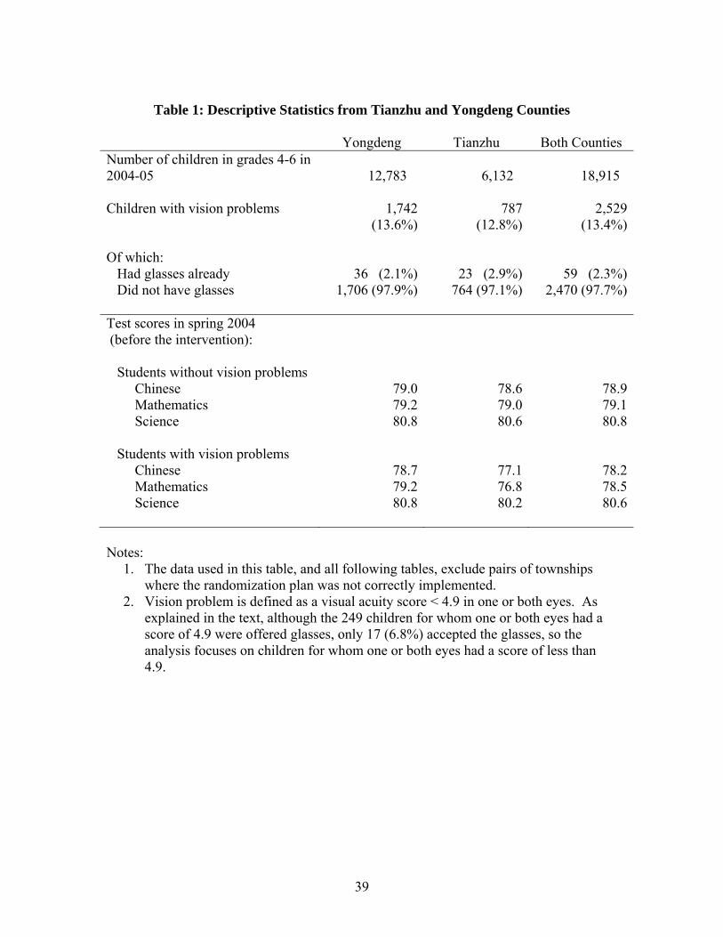
39

Table 1: Descriptive Statistics from Tianzhu and Yongdeng Counties

Yongdeng Tianzhu Both Counties Number of children in grades 4-6 in 2004-05 12,783 6,132 18,915 Children with vision problems 1,742

(13.6%)787

(12.8%) 2,529

(13.4%) Of which: Had glasses already 36 (2.1%) 23 (2.9%) 59 (2.3%) Did not have glasses 1,706 (97.9%) 764 (97.1%) 2,470 (97.7%) Test scores in spring 2004 (before the intervention):

Students without vision problems Chinese 79.0 78.6 78.9 Mathematics 79.2 79.0 79.1 Science 80.8 80.6 80.8 Students with vision problems Chinese 78.7 77.1 78.2 Mathematics 79.2 76.8 78.5 Science 80.8 80.2 80.6 Notes:

1. The data used in this table, and all following tables, exclude pairs of townships where the randomization plan was not correctly implemented.

2. Vision problem is defined as a visual acuity score < 4.9 in one or both eyes. As explained in the text, although the 249 children for whom one or both eyes had a score of 4.9 were offered glasses, only 17 (6.8%) accepted the glasses, so the analysis focuses on children for whom one or both eyes had a score of less than 4.9.

40

Table 2: Implementation of Gansu Vision Intervention Project

Yongdeng Tianzhu Both Counties Students in grades 4-6 in 2004-05 with vision problems

1,742 787 2,529

Of which: In control schools 889 112 1,001 In program schools 853 675 1,528 Students in program schools who: Accepted the offer to receive glasses

649 417 1,066

Did not accept the offer to receive glasses

204 258 462

Reasons given for not accepting glasses:

Household head refused 91 54 145 Child refused 38 42 80 Cannot adjust to glasses 0 58 58 Eye disease 1 0 11 11 Optometrist not available 7 27 34 Eye disease 2 30 33 63 Eye problem cannot be corrected by glasses

0 5 5

Eye disease 3 0 1 1 Vision not correctable(?) 19 0 19 Child is handicapped 2 0 2 Missing 17 27 44 Notes:

1. The data used in this table, and all following tables, exclude pairs of townships where the randomization plan was not correctly implemented.

2. Vision problem is defined as a visual acuity score < 4.9 in one or both eyes.

41

Table 3: Check for Pre-Program Differences across Treatment and Control Groups (Differences in Spring 2004 Scores)

Dependent Variable Explanatory Variables Chinese Math Science Average

Equation (1): School Random Effects, Only Students with Poor Vision N = 2,491 Treatment Township (β) 0.045

(0.094) [0.712]

-0.042 (0.089) [0.726]

0.001 (0.074) [0.988]

0.003 (0.095) [0.952]

Equation (2): School Random Effects, All Students N = 18,602 Poor Vision (π) 0.040

(0.030) 0.089** (0.036)

0.065* (0.035)

0.077*** (0.028)

Treatment Township (τ) 0.028 (0.064)

0.007 (0.066)

0.083 (0.054)

0.046 (0.069)

Poor Vision×Treatment Township (β) 0.014 (0.044) [0.816]

-0.076 (0.058) [0.264]

-0.072 (0.053) [0.182]

-0.053 (0.048) [0.326]

Equation (2): School Fixed Effects, All Students N = 18,602 Poor Vision (π) 0.043

(0.030) 0.089** (0.036)

0.066* (0.036)

0.078** (0.028)

Treatment Township (τ) Not identified

Not identified

Not identified

Not identified

Poor Vision×Treatment Township (β) 0.015 (0.044) [0.790]

-0.075 (0.059) [0.268]

-0.072 (0.053) [0.194]

-0.052 (0.049) [0.338]

Notes: 1. Constant terms and strata dummy variables are not shown (to reduce clutter).

2. Standard errors in parentheses; wild bootstrap p-values in brackets. Random effects models include school random effects, and fixed effects models include school fixed effects. Both models allow for heteroscedasticity, including correlation (clustering) among observations within the same township, of unknown form for the individual level error term. Asterisks denote statistical significance: * 10% level, ** 5% level, *** 1% level.

42

Table 4: Estimated Program Effect After One Year: Conditional on 2004 Scores

Dependent Variable Explanatory Variables Chinese Math Science Average

Equation (1): School Random Effects, Only Students with Poor Vision N = 2,474 2004 Chinese Score 0.172*** 0.193*** 0.162*** 0.219*** (0.047) (0.042) (0.041) (0.045) 2004 Math Score 0.125*** 0.169*** 0.213*** 0.212*** (0.022) (0.047) (0.043) (0.030) 2004 Science Score 0.138*** 0.087*** 0.134*** 0.149*** (0.022) (0.031) (0.032) (0.028) Treatment Township (β) 0.091

(0.078) [0.374]

0.097 (0.084) [0.454]

0.186*** (0.055) [0.016]

0.156** (0.077) [0.214]

Equation (2): School Random Effects, All Students N = 18,504 2004 Chinese Score 0.200*** 0.169*** 0.126*** 0.206*** (0.029) (0.026) (0.016) (0.023) 2004 Math Score 0.111*** 0.184*** 0.209*** 0.209*** (0.014) (0.031) (0.045) (0.027) 2004 Science Score 0.159*** 0.109*** 0.194*** 0.192*** (0.021) (0.018) (0.023) (0.019) Poor Vision (π) -0.043

(0.038) -0.020 (0.028)

0.011 (0.034)

-0.022 (0.030)

Treatment Township (τ) -0.059 (0.060)

-0.008 (0.050)

0.037 (0.061)

-0.013 (0.063)

Poor Vision×Treatment Township (β)

0.117** (0.051) [0.096]

0.072 (0.055) [0.234]

0.071 (0.044) [0.132]

0.108** (0.049) [0.034]

Equation (2): School Fixed Effects, All Students N = 18,504 2004 Chinese Score 0.199*** 0.169*** 0.125*** 0.206*** (0.029) (0.027) (0.016) (0.023) 2004 Math Score 0.110*** 0.185*** 0.208*** 0.209*** (0.014) (0.031) (0.045) (0.027) 2004 Science Score 0.156*** 0.108*** 0.191*** 0.189*** (0.021) (0.018) (0.023) (0.018) Poor Vision (π) -0.043

(0.038) -0.021 (0.029)

0.011 (0.034)

-0.022 (0.030)

Treatment Township (τ) Unidentified Unidentified Unidentified UnidentifiedPoor Vision×Treatment Township (β)

0.116** (0.051) [0.024]

0.072 (0.056) [0.238]

0.070 (0.044) [0.170]

0.107** (0.049) [0.052]

Notes: 1. Constant terms and strata dummy terms are not shown (to reduce clutter).

2. Standard errors in parentheses; wild bootstrap p-values in brackets. Random (fixed) effects models include school random (fixed) effects. All models allow for heteroscedasticity, including correlation (clustering) among observations within the same township, of unknown form for the individual level error term. Asterisks denote statistical significance: * 10% level, ** 5% level, *** 1% level.

43

Table 5: Effect of Eyeglasses After One Year: IV Results Conditional on 2004 Scores

Dependent Variable Explanatory Variables Chinese Math Science Average

Equation (1): School Random Effects, Only Students with Poor Vision N = 2,474 2004 Chinese Score 0.171*** 0.193*** 0.162*** 0.218*** (0.046) (0.040) (0.038) (0.043) 2004 Math Score 0.123*** 0.169*** 0.211*** 0.210*** (0.022) (0.047) (0.044) (0.030) 2004 Science Score 0.137*** 0.088*** 0.136*** 0.149*** (0.022) (0.031) (0.031) (0.028) Has Eyeglasses (β)

0.130 (0.109)

0.137 (0.120)

0.261*** (0.073)

0.221** (0.109)

Equation (2): School Random Effects, All Students N = 18,503 2004 Chinese Score 0.200*** 0.169*** 0.126*** 0.206*** (0.029) (0.026) (0.015) (0.023) 2004 Math Score 0.110*** 0.184*** 0.209*** 0.209*** (0.013) (0.030) (0.044) (0.027) 2004 Science Score 0.159*** 0.109*** 0.195*** 0.192*** (0.020) (0.018) (0.022) (0.018) Poor Vision (π) -0.041

(0.038) -0.021 (0.029)

0.008 (0.033)

-0.023 (0.030)

Has Eyeglasses (β) 0.162** (0.074)

0.103 (0.080)

0.107* (0.060)

0.154** (0.071)

Equation (2): School Fixed Effects, All Students N = 18,503 2004 Chinese Score 0.199*** 0.169*** 0.126*** 0.206*** (0.028) (0.026) (0.016) (0.023) 2004 Math Score 0.110*** 0.185*** 0.208*** 0.209*** (0.013) (0.030) (0.044) (0.026) 2004 Science Score 0.156*** 0.108*** 0.191*** 0.189*** (0.020) (0.018) (0.022) (0.018) Poor Vision (π) -0.044

(0.038) -0.022 (0.028)

0.010 (0.034)

-0.023 (0.030)

Has Eyeglasses (β)

0.166** (0.074)

0.103 (0.080)

0.100 (0.063)

0.153** (0.071)

Notes: 1. Constant terms and strata dummy terms are not shown (to reduce clutter).

2. Standard errors in parentheses; pairs cluster bootstrap p-values in brackets. Random (fixed) effects models include school random (fixed) effects. All models allow for heteroscedasticity, including correlation (clustering) among observations within the same township, of unknown form for the individual level error term. Asterisks denote statistical significance: * 10% level, ** 5% level, *** 1% level.

3. The instrumental variable for having eyeglasses is a dummy variable that indicates that one has been selected into the program and has poor vision.

44

Table 6: Estimated Program Effects for Students with Good Vision

Dependent Variable Explanatory Variables Chinese Math Science Average Equation (1): School Random Effects, Only Students with Good Vision N = 16,031

Treatment Township (β) -0.046 (0.077) [0.736]

-0.002 (0.066) [0.950]

0.048 (0.088) [0.734]

-0.001 (0.091) [0.960]

Equation (1): School Random Effects, Only Students with Good Vision N = 16,0302004 Chinese Score 0.206***

(0.029) 0.164*** (0.026)

0.120*** (0.015)

0.204*** (0.021)

2004 Math Score 0.108*** (0.013)

0.187*** (0.032)

0.208*** (0.046)

0.208*** (0.028)

2004 Science Score 0.164*** (0.022)

0.112*** (0.018)

0.205*** (0.023)

0.199*** (0.019)

Treatment Township (β) -0.065 (0.060) [0.480]

-0.015 (0.050) [0.808]

0.029 (0.063) [0.776]

-0.022 (0.064) [0.856]

Notes: 1. Constant terms and strata dummy terms are not shown (to reduce clutter).

2. Standard errors in parentheses; wild bootstrap p-values in brackets. All models include school random effects. All models allow for heteroscedasticity, including correlation (clustering) among observations within the same township, of unknown form for the individual level error term. Asterisks denote statistical significance: * 10% level, ** 5% level, *** 1% level.

Table 7: Falsification Test: “Effect” of Program in 2003-04 School Year

Dependent Variable (2004 test scores) Explanatory Variables Chinese Math Science Average

Equation (2): School Random Effects, All Students N = 18,600 2003 Chinese Score 0.387*** 0.215*** 0.125*** 0.286*** (0.012) (0.016) (0.010) (0.008) 2003 Math Score 0.178*** 0.355*** 0.121*** 0.257*** (0.014) (0.024) (0.015) (0.011) 2003 Science Score 0.130*** 0.111*** 0.425*** 0.260*** (0.012) (0.016) (0.025) (0.018) Poor Vision (π) -0.019

(0.019) 0.036

(0.032) 0.030

(0.029) 0.018

(0.015) Treatment Township (τ) -0.017

(0.032) -0.037 (0.032)

0.027 (0.022)

-0.010 (0.028)

Poor Vision×Treatment Township (β) 0.055 (0.036) [0.186]

-0.046 (0.046) [0.388]

-0.053 (0.041) [0.228]

-0.017 (0.030) [0.576]

Notes: Same notes as those given for Table 6.

45

Table 8 Effect of Eyeglasses After One Year: IV Results Using Full Sample

Dependent Variable Explanatory Variables Chinese Math Science Average

Equation (1): School Random Effects, Only Students with Poor Vision N = 4,293 2004 Chinese Score 0.160*** 0.176*** 0.162*** 0.191*** (0.042) (0.040) (0.038) (0.046) 2004 Math Score 0.116*** 0.160*** 0.211*** 0.199*** (0.022) (0.036) (0.043) (0.029) 2004 Science Score 0.154*** 0.092*** 0.136*** 0.165*** (0.023) (0.023) (0.031) (0.025) Has Eyeglasses (β)

-0.078 (0.138)

-0.082 (0.160)

0.026 (0.126)

-0.051 (0.161)

Equation (2): School Random Effects, All Students N = 32,587 2004 Chinese Score 0.208*** 0.185*** 0.128*** 0.217*** (0.027) (0.026) (0.015) (0.025) 2004 Math Score 0.111*** 0.179*** 0.201*** 0.204*** (0.017) (0.029) (0.039) (0.031) 2004 Science Score 0.155*** 0.103*** 0.205*** 0.192*** (0.015) (0.014) (0.022) (0.015) Poor Vision (π) -0.041

(0.043) -0.028 (0.041)

0.024 (0.043)

-0.020 (0.043)

Has Eyeglasses (β)

0.158* (0.088)

0.106 (0.103)

0.033 (0.094)

0.126 (0.096)

Equation (2): School Fixed Effects, All Students N = 32,587 2004 Chinese Score 0.206*** 0.184*** 0.127*** 0.216*** (0.027) (0.026) (0.015) (0.025) 2004 Math Score 0.110*** 0.179*** 0.200*** 0.203*** (0.018) (0.029) (0.039) (0.031) 2004 Science Score 0.153*** 0.101*** 0.201*** 0.190*** (0.015) (0.014) (0.022) (0.015) Poor Vision (π) -0.056

(0.045) -0.035 (0.041)

0.020 (0.044)

-0.029 (0.044)

Has Eyeglasses (β)

0.184** (0.092)

0.119 (0.104)

0.037 (0.096)

0.140 (0.098)

Notes: 1. Constant terms and strata dummy terms are not shown (to reduce clutter).

2. Standard errors in parentheses; pairs cluster bootstrap p-values in brackets. Random (fixed) effects models include school random (fixed) effects. All models allow for heteroscedasticity, including correlation (clustering) among observations within the same township, of unknown form for the individual level error term. Asterisks denote statistical significance: * 10% level, ** 5% level, *** 1% level.

3. The instrumental variable for having eyeglasses is a dummy variable that indicates that one has been selected into the program and has poor vision.

46

Table 9: Interaction Effects Between Program, Visual Acuity and 2004 Test Scores Explanatory Variables Dependent Variable:

Average Test Score Equation (1): School Random Effects, Only Students with Poor Vision N = 2,474

2004 Chinese Score 0.219*** (0.046)

0.212*** (0.029)

0.148*** (0.028) 0.171**

(0.077) [0.130]

0.246*** (0.034)

0.241*** (0.035)

0.174*** (0.030) 0.136*

(0.079) [0.236]

2004 Math Score 2004 Science Score Treatment Township (β)

Very Poor Vision 0.052 (0.040)

--

Very Poor Vision × Treatment Township -0.082 (0.069) [0.282]

--

Avg. Test Score 2004 × Treatment Township -- -0.106 (0.092) [0.284]

Equation (2): School Random Effects, All Students N = 18,478 2004 Chinese Score 0.208***

(0.023) 0.209*** (0.027)

0.191*** (0.019) -0.025 (0.033) -0.011 (0.063)

0.200*** (0.029)

0.202*** (0.030)

0.185*** (0.024) -0.012 (0.029) -0.007 (0.061)

2004 Math Score 2004 Science Score Poor Vision (π) Treatment Township (τ)

Poor Vision × Treatment Township (β) 0.119** (0.051) [0.054]

0.081* (0.043) [0.092]

Very Poor Vision 0.030 (0.053)

--

Very Poor Vision × Treatment Township -0.064 (0.077) [0.410]

--

2004 Avg. Test Score × Treatment Township -- 0.033 (0.079)

2004 Avg. Test Score × Poor Vision -- 0.068** (0.032)

2004 Avg. Test Score × Poor Vision × Treatment Township

-0.166*** (0.055) [0.014]

Notes: 1. Constant terms and strata dummy terms are not shown (to reduce clutter). 2. Standard errors in parentheses; wild bootstrap p-values in brackets. All models

allow for heteroscedasticity, including correlation (clustering) among observations within the same township, of unknown form for the individual level error term. Asterisks denote statistical significance: * 10% level, ** 5% level, *** 1% level.

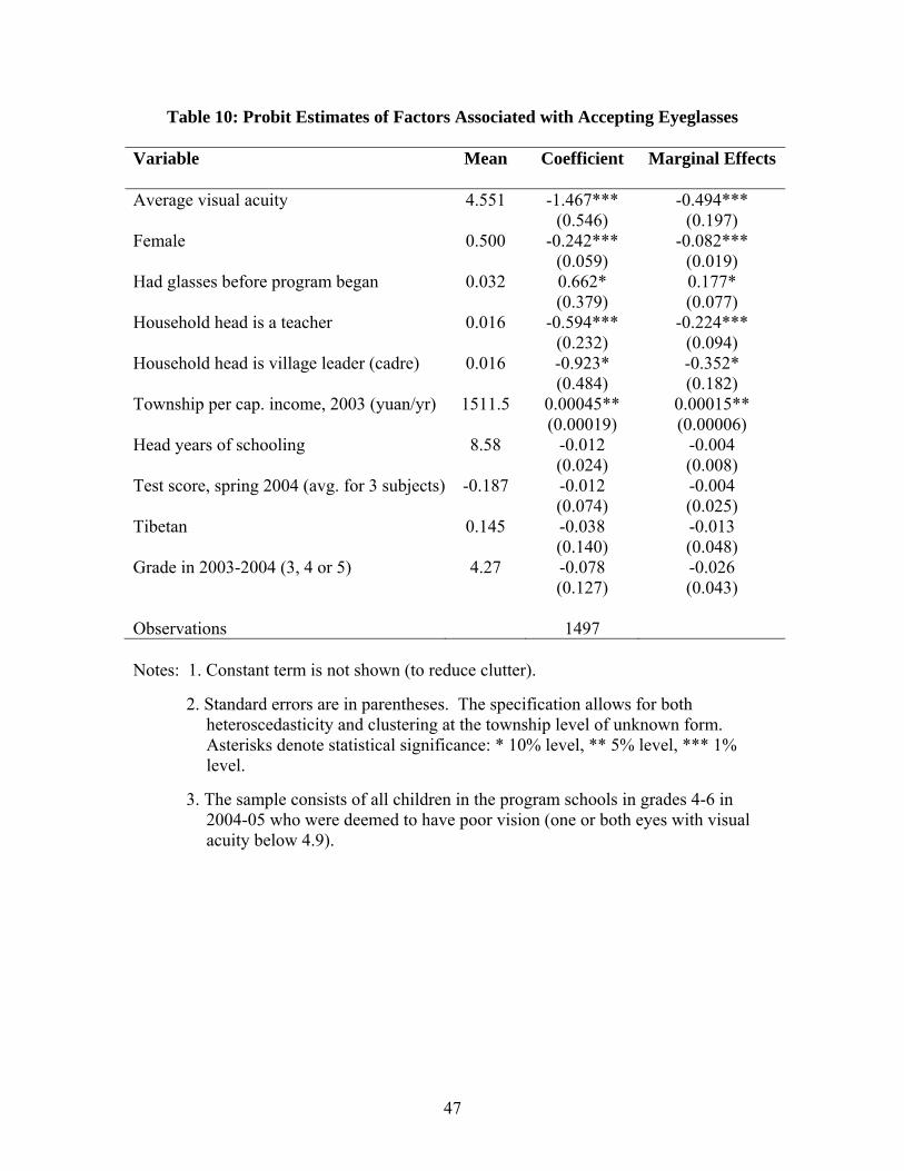
47

Table 10: Probit Estimates of Factors Associated with Accepting Eyeglasses

Variable Mean Coefficient Marginal Effects Average visual acuity 4.551 -1.467***

(0.546) -0.494***

(0.197) Female 0.500 -0.242***

(0.059) -0.082***

(0.019) Had glasses before program began 0.032 0.662*

(0.379) 0.177* (0.077)

Household head is a teacher 0.016 -0.594*** (0.232)

-0.224*** (0.094)

Household head is village leader (cadre) 0.016 -0.923* (0.484)

-0.352* (0.182)

Township per cap. income, 2003 (yuan/yr) 1511.5 0.00045** (0.00019)

0.00015** (0.00006)

Head years of schooling 8.58 -0.012 (0.024)

-0.004 (0.008)

Test score, spring 2004 (avg. for 3 subjects) -0.187 -0.012 (0.074)

-0.004 (0.025)

Tibetan 0.145 -0.038 (0.140)

-0.013 (0.048)

Grade in 2003-2004 (3, 4 or 5) 4.27 -0.078 (0.127)

-0.026 (0.043)

Observations 1497 Notes: 1. Constant term is not shown (to reduce clutter).

2. Standard errors are in parentheses. The specification allows for both heteroscedasticity and clustering at the township level of unknown form. Asterisks denote statistical significance: * 10% level, ** 5% level, *** 1% level.

3. The sample consists of all children in the program schools in grades 4-6 in 2004-05 who were deemed to have poor vision (one or both eyes with visual acuity below 4.9).

48

Table 11: Mother’s Assessment of Vision and Actual Visual Acuity (children age 8-15 who were enrolled in primary school in 2004)

Measured

Acuity Mother’s Assessment

Very Bad Bad Fair Good Very good Don’t KnowGood (≥ 5.0) 1 4 92 251 367 4 Fair (4.8-4.99) 0 0 18 29 52 0 Poor (< 4.8) 1 7 17 14 29 1 Source: Gansu Survey of Children and Families.

Table 12: Children’s Reports of Vision Problems, by Actual Visual Acuity (children age 8-15 who were enrolled in primary school in 2004)

Measured Child Reports of Vision Problems

Visual Acuity

Difficulty seeing blackboard (%)

Trouble doing homework due to poor vision (%)

Felt pain in eyes when studying at home in

dim light (%) Good (≥ 5.0) 8.5 6.7 19.1 Fair (4.8-4.99) 7.1 7.1 21.2 Poor (< 4.8) 30.4 26.1 29.0 Source: Gansu Survey of Children and Families.

49

Table 13: Determinants of Student Wearing of Eyeglasses (from 2004 Gansu Survey of Children and Families)

(1) (2) (3) (4) (5) (6) VARIABLES Coefficient Estimates from Probit Specification Marginal Effects Visual acuity -1.329*** -0.858** -0.852** -0.670 -0.783* -0.0196 (best eye) (0.374) (0.412) (0.420) (0.423) (0.417) (0.0120) Female -0.228 -0.210 -0.228 -0.145 -0.155 -0.00396 (0.169) (0.177) (0.173) (0.173) (0.173) (0.00417) Age (years) 0.0849** 0.0902*** 0.0861** 0.101*** 0.101*** 0.00253** (0.0339) (0.0341) (0.0346) (0.0375) (0.0386) (0.00106) Father’s education -0.0210 -0.0114 -0.0104 -0.000136 0.00228 5.69e-05 (0.0325) (0.0341) (0.0334) (0.0365) (0.0375) (0.000930) Mother’s education 0.0919*** 0.0895*** 0.0936*** 0.0851** 0.0722* 0.00180* (0.0316) (0.0326) (0.0331) (0.0364) (0.0372) (0.00105) Log p.c. expend. 0.553*** 0.515*** 0.530*** 0.497** 0.463** 0.0116** (0.184) (0.190) (0.189) (0.204) (0.201) (0.00562) Mother assessment 0.898*** 0.887*** 0.858*** 0.809*** 0.0508 of child’s vision (0.326) (0.329) (0.307) (0.298) (0.0364) Father assessment 0.603 0.605 0.558 0.542 0.0247 of child’s vision (0.380) (0.385) (0.357) (0.364) (0.0251) Estimated cost of -0.00366* -0.00375* -0.00451** -0.000113 glasses (0.00215) (0.00218) (0.00225) (7.37e-05) Estimated distance 0.00164 0.000704 0.000869 2.17e-05 to buy glasses (0.00422) (0.00392) (0.00388) (9.75e-05) Parent wears 0.955*** 0.962*** 0.0678 glasses (0.322) (0.318) (0.0439) Village literacy rate 1.300** 0.0325* (0.645) (0.0171) Constant -0.392 -2.710 -2.668 -3.679 -3.890 (2.360) (2.732) (2.751) (2.731) (2.898) Observations 921 921 921 921 921 921

Notes: 1. Standard errors are in parentheses. The specification allows for both hetero-

scedasticity and clustering at the village level of unknown form. Asterisks denote statistical significance: * 10% level, ** 5% level, *** 1% level.

2. Estimated cost of glasses and distance to buy glasses are medians of parental

reports.

50

Appendix I: Impact of Measurement Error in the Poor Vision (PV) Variable

This appendix shows that random measurement error in the poor vision variable will lead to underestimation of program effects in estimation of equation (2). Let PV* be the (unobserved) true indicator of whether a child has poor vision, and let PV denote the observed value of that variable. Thus PV = PV* + ε, where ε is the measurement error. Since both PV and PV* are dummy variables, ε will clearly be correlated with PV*, so this is not classical measurement error.

Assume that both types of measurement error (PV = 0 when PV* = 1 and PV = 1 when PV* = 0) occur with the same frequency, denoted by θ. Thus there are three possibilities:

Frequency Value of PV* Value of PV Value of ε

1-2θ (no error) 1 or 0 Same as PV* 0 θ 0 1 1 θ 1 0 -1 The assumption that both types of errors occur with the same frequency is plausible if the error in the underlying visual acuity variable is random and the density of the distribution of that variable is similar on both sides of the cutoff point (4.8), and the latter is approximately correct. Measurement error alters equation (2) as follows:

T = α + πPV* + τP + βPV*P + u

= α + π(PV - ε) + τP + β(PV – ε)*P + u

= α + πPV + τP + βPV*P + (u – πε – βεP) Bias in OLS estimation of β will be primarily determined by whether the interaction term PV*P is correlated with the composite error term (u – πε – βεP). Focusing on bias due to measurement error, this will be determined by whether PV*P is correlated with πε + βεP. Covariance formulas imply Cov(πε + βεP, PV*P) = πCov(ε, PV*P) + βCov(εP, PV*P). The following derivations show that Cov(ε, PV*P) = Cov(εP, PV*P) = θE[P]:

Cov(ε, PV*P) = E[(ε – E[ε])(PV*P – E[PV*P])] = E[ε(PV*P – E[PV*P])]

= E[εPV*P] – E[ε]E[PV*P] = E[εPV*P]

= Prob[ε = 0]×E[εPV*P| ε = 0] + Prob[ε = -1]×E[εPV*P| ε = -1] + Prob[ε = 1]× E[εPV*P| ε = 1] = (1 – 2θ)×0 + θ×(-1×0×E[P]) + θ×(1×1×E[P])

= 0 + 0 + θE[P] > 0

Cov(εP, PV*P) = E[(εP – E[εP])(PV*P – E[PV*P])] = E[(εP – E[ε]×E[P])(PV*P – E[PV*P])]

51

= E[εP(PV*P – E[PV*P])] = E[εPV*P2 – E[εP]E[PV*P])]

= E[εPV*P – E[ε]E[P]E[PV*P])] = E[εPV*P] = θE[P] > 0

Thus we have:

Cov(πε + βεP, PV*P) = πCov(ε, PV*P) + βCov(εP, PV*P) = (π + β)θE[P]

This derivation has two implications. First, as measurement error decreases (θ → 0), this correlation goes to zero and so bias goes to zero. Second, it is reasonable to assume that π = - β. Quite simply, if we expect a child with poor vision to score lower on tests by a factor of π (note that π < 0), then providing that child with glasses should remove the problem, which implies an impact of the same magnitude but in the opposite direction (β > 0). Thus implies that the two terms in the bias tend to cancel each other out. Note that the fact that π may be estimated with bias does not matter for this derivation, which is based on the true underlying value of π, not an estimate of π.

52

Appendix II: Additional Tables

Table A.1: Check for Pre-Program Differences across Treatment and Control Groups, Including Township Pairs where Randomization Was not Correctly Implemented

(Differences in Spring 2004 Scores)

Dependent Variable Explanatory Variables Chinese Math Science Average

Equation (1): School Random Effects, Only Students with Poor Vision N = 4,453 Treatment Township (β) -0.129

(0.103) [0.476]

-0.172* (0.098) [0.262]

-0.071 (0.091) [0.584]

-0.144 (0.109) [0.398]

Equation (2): School Random Effects, All Students N = 33,679 Poor Vision (π) 0.025

(0.022) 0.085*** (0.024)

0.041 (0.027)

0.059** (0.026)

Treatment Township (τ) -0.100 (0.084)

-0.069 (0.077)

-0.018 (0.078)

-0.072 (0.093)

Poor Vision×Treatment Township (β) 0.010 (0.035) [0.804]

-0.091** (0.041) [0.070]

-0.031 (0.045) [0.516]

-0.044 (0.038) [0.268]

Equation (2): School Fixed Effects, All Students N = 33,679 Poor Vision (π) 0.025

(0.022) 0.085*** (0.025)

0.041 (0.028)

0.060** (0.026)

Treatment Township (τ) Not identified

Not identified

Not identified

Not identified

Poor Vision×Treatment Township (β) 0.010 (0.035) [0.806]

-0.091** (0.042) [0.076]

-0.032 (0.045) [0.508]

-0.045 (0.039) [0.276]

Notes: 1. Constant terms and strata dummy variables are not shown (to reduce clutter).

2. Standard errors in parentheses; wild bootstrap p-values in brackets. Random effects models include school random effects, and fixed effects models include school fixed effects. Both models allow for heteroscedasticity, including correlation (clustering) among observations within the same township, of unknown form for the individual level error term. Asterisks denote statistical significance: * 10% level, ** 5% level, *** 1% level.

53

Table A.2: Estimated Program Effect After One Year (not conditional on 2004 test scores)

Dependent Variable Explanatory Variables Chinese Math Science Average

Equation (1): School Random Effects, Only Students with Poor Vision N = 2,474 Treatment Township (β) 0.097

(0.094) [0.462]

0.098 (0.089) [0.458]

0.191** (0.083) [0.152]

0.161 (0.098) [0.294]

Equation (2): School Random Effects, All Students N = 18,505 Poor Vision (π) -0.015

(0.029) 0.010

(0.030) 0.047

(0.032) 0.018

(0.023)

Treatment Township (τ) -0.039 (0.076)

0.005 (0.064)

0.056 (0.085)

0.008 (0.088)

Poor Vision×Treatment Township (β) 0.100** (0.050) [0.060]

0.054 (0.062) [0.404]

0.043 (0.049) [0.414]

0.081 (0.055) [0.174]

Equation (2): School Fixed Effects, All Students N = 18,505 Poor Vision (π) -0.014

(0.029) 0.010

(0.030) 0.047

(0.032) 0.018

(0.023)

Treatment Township (τ) Not identified

Not identified

Not identified

Not identified

Poor Vision×Treatment Township (β) 0.099* (0.050) [0.058]

0.054 (0.063) [0.418]

0.042 (0.050) [0.414]

0.081 (0.055) [0.182]

Notes: 1. Constant terms and strata dummy variables are not shown (to reduce clutter).

2. Standard errors in parentheses; wild bootstrap p-values in brackets. Random effects models include school random effects, and fixed effects models include school fixed effects. Both models allow for heteroscedasticity, including correlation (clustering) among observations within the same township, of unknown form for the individual level error term. Asterisks denote statistical significance: * 10% level, ** 5% level, *** 1% level.