Visualization in the integrated SimPhoNy multiscalesimulation framework

Joan Adlera, Sampo Kuljub, Jari Hyvaluomab, Keijo Mattilac,d, Kit Choie,Ioannis Tziakose, Didrik Pintee, G. A. Garcıaf, Y. Makushokf, V. Makushokf,

J. Lamaf, G. Roman-Perezf, Adham Hashibong, Mehdi Sadeghig, NathanFrankling, Amihai Silvermanh

aTechnion - IIT, Haifa, Israel, 32000bNatural Resources Institute Finland (Luke), FI-31600 Jokioinen, FinlandcDepartment of Physics and Nanoscience Center, University of Jyvaskyla,

P.O. Box 35 (YFL), FI-40014 University of Jyvaskyla, FinlanddDepartment of Physics, Tampere University of Technology,

P.O. Box 692, FI-33101 Tampere, FinlandeEnthought Ltd.,Cambridge, United Kingdom

fSgenia, Madrid, SpaingIWM

hCIS Department, Technion -IIT, Haifa, Israel, 32000

Abstract

We describe three distinct approaches to visualization for multiscale materi-

als modelling research. These have been developed with the framework of the

SimPhoNy FP7 EU-project, and complement each other in their requirements

and possibilities. All have been integrated via wrappers to one or more of the

simulation approaches within the SimPhoNy project. In this manuscript we de-

scribe and contrast their features. Together they cover visualization needs from

electronic to macroscopic scales and are suited to simulations made on personal

computers, workstations or advanced High Performance parallel computers. Ex-

amples as well as recommendations for future calculations are presented.

Keywords: visualization, atomistic, electronic charge density, fluid

2010 MSC: 00-01, 99-00

Email address: phr76ja@tx.technion.ac.il (Joan Adler)

Preprint submitted to Computer Physics Communications January 24, 2017

1. Introduction - summary of SimPhoNy concepts and structure

Progress in modelling, e.g. in the field of materials research, requires ev-

ermore detailed considerations of a system or phenomena under investigation.

This may be accomplished by resorting to multi-scale or multi-physics mod-

elling. The related models are complex to a degree which rarely allows analyti-5

cal treatment and, thus, numerical simulations are routinely used for obtaining

approximate solutions. However, an in-house implementation of multi-scale or

multi-physics simulators is laborious and may compromise the cost-effectiveness

of computational experiments in comparison to laboratory experiments. The sit-

uation is particularly demanding when short development cycles are critical: a10

new application may require implementation of new features which, in the case

of complex simulators, can take more time to complete than a rapid reaction

permits.

A solution is to rely on well-established, specialized simulators which alone

can resolve only part of the system or phenomena at hand. Two or more of15

these simulators are then set up to cooperate in an effort to treat the whole

system at once. Here the main challenges are configuration and operation of

the various simulators and orchestration of necessary data exchange between

the simulators.

The SimPhoNy integrated framework (freely available via [1]) is developed20

specifically to address these difficulties and, above all, to facilitate simulation of

systems requiring multi-scale or multi-physics modelling. The principal design

aspects of SimPhoNy include the Common Universal Basic Attributes (CUBA)

and the Common Universal Data Structures (CUDS): all physical and compu-

tational variables or parameters are expressed using CUBA. In addition, more25

complex data types are necessary for configuring simulations and for repre-

senting computational data sets (e.g. mesh- or particle-based data sets) in a

standard fashion. These data types are specified by CUDS and the definitions

are build on top of CUBA.

The above design features are complemented by the specification of simple30

2

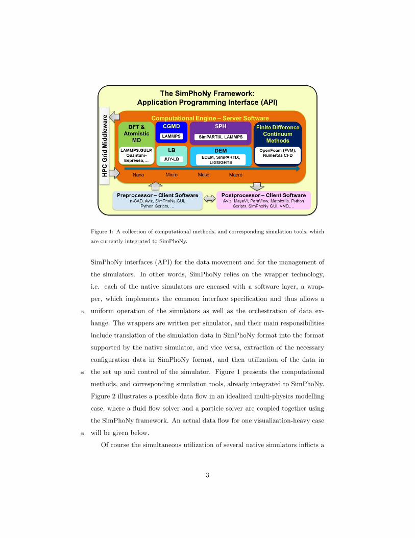
Figure 1: A collection of computational methods, and corresponding simulation tools, which

are currently integrated to SimPhoNy.

SimPhoNy interfaces (API) for the data movement and for the management of

the simulators. In other words, SimPhoNy relies on the wrapper technology,

i.e. each of the native simulators are encased with a software layer, a wrap-

per, which implements the common interface specification and thus allows a

uniform operation of the simulators as well as the orchestration of data ex-35

hange. The wrappers are written per simulator, and their main responsibilities

include translation of the simulation data in SimPhoNy format into the format

supported by the native simulator, and vice versa, extraction of the necessary

configuration data in SimPhoNy format, and then utilization of the data in

the set up and control of the simulator. Figure 1 presents the computational40

methods, and corresponding simulation tools, already integrated to SimPhoNy.

Figure 2 illustrates a possible data flow in an idealized multi-physics modelling

case, where a fluid flow solver and a particle solver are coupled together using

the SimPhoNy framework. An actual data flow for one visualization-heavy case

will be given below.45

Of course the simultaneous utilization of several native simulators inflicts a

3

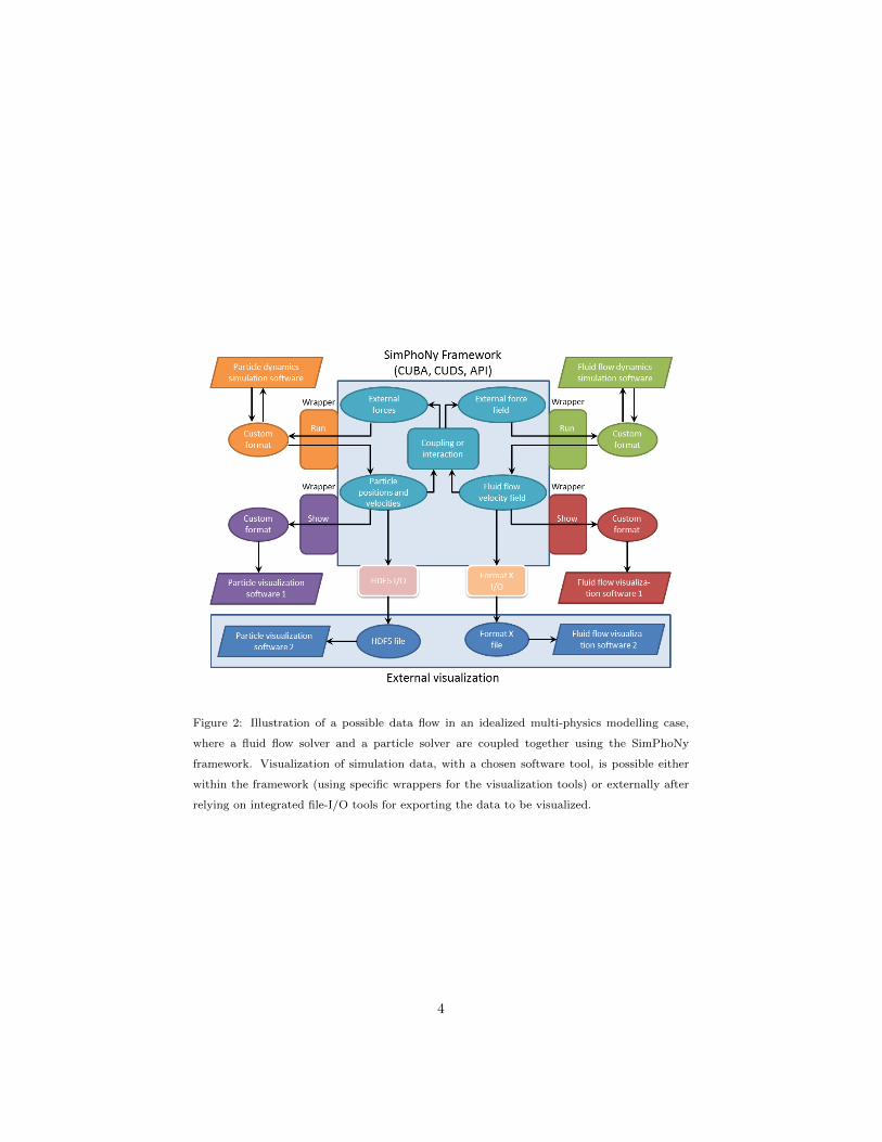
Figure 2: Illustration of a possible data flow in an idealized multi-physics modelling case,

where a fluid flow solver and a particle solver are coupled together using the SimPhoNy

framework. Visualization of simulation data, with a chosen software tool, is possible either

within the framework (using specific wrappers for the visualization tools) or externally after

relying on integrated file-I/O tools for exporting the data to be visualized.

4

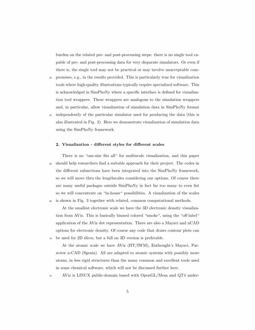
burden on the related pre- and post-processing steps: there is no single tool ca-

pable of pre- and post-processing data for very disparate simulators. Or even if

there is, the single tool may not be practical or may involve unacceptable com-

promises, e.g., in the results provided. This is particularly true for visualization50

tools where high-quality illustrations typically require specialized software. This

is acknowledged in SimPhoNy where a specific interface is defined for visualiza-

tion tool wrappers. These wrappers are analogous to the simulation wrappers

and, in particular, allow visualization of simulation data in SimPhoNy format

independently of the particular simulator used for producing the data (this is55

also illustrated in Fig. 2). Here we demonstrate visualization of simulation data

using the SimPhoNy framework.

2. Visualization - different styles for different scales

There is no “one-size fits all“ for multiscale visualization, and this paper

should help researchers find a suitable approach for their project. The codes in60

the different subsections have been integrated into the SimPhoNy framework,

so we will move thru the lengthscales considering our options. Of course there

are many useful packages outside SimPhoNy in fact far too many to even list

so we will concentrate on “in-house“ possibilities. A visualization of the scales

is shown in Fig. 3 together with related, common computational methods.65

At the smallest electronic scale we have the 3D electronic density visualiza-

tion from AViz. This is basically binned colored “smoke“, using the “off-label“

application of the AViz dot representation. There are also a Mayavi and nCAD

options for electronic density. Of course any code that draws contour plots can

be used for 2D slices, but a full on 3D version is preferable.70

At the atomic scale we have AViz (IIT/IWM), Enthought’s Mayavi, Par-

aview n-CAD (Sgenia). All are adapted to atomic systems with possibly more

atoms, in less rigid structures than the many common and excellent tools used

in some chemical software, which will not be discussed further here.

AViz is LINUX public-domain based with OpenGL/Mesa and QT4 under-75

5

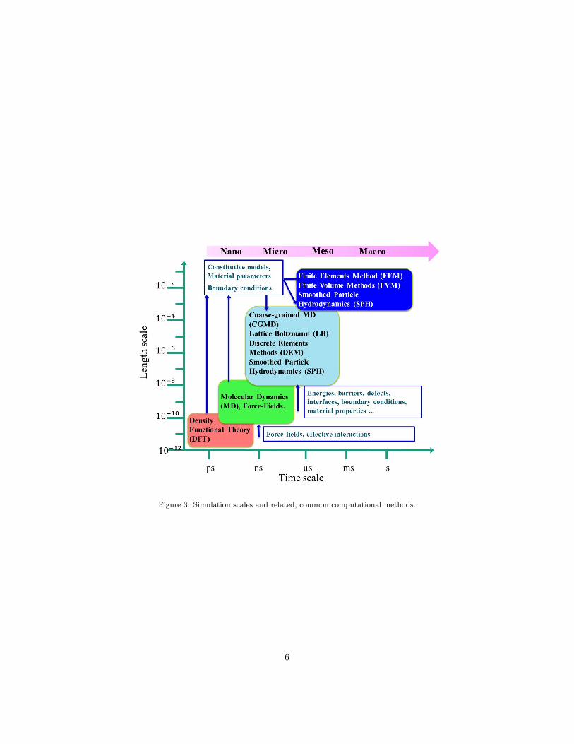
Figure 3: Simulation scales and related, common computational methods.

6

pinnings, Enthought’s Mayavi2 and Paraview are common to LINUX, Mac and

Windows and are vtk based under the permissive BSD license, whereas n-CAD

is Microsoft windows and proprietry.

When we model at the the micro/meso/macro scale we often need to visu-

alize fluids. This is a well-researched field, especially in the context of CFD80

(Computational Fluid Mechanics), with both many codes and many approaches

for both scalar and vector fluid flow. Several SimPhoNy applications fall into

this category, and examples are given below. At the micro/meso scale there are

also visualization needs for solid objects which are well satisfied by many codes,

but not particularly relevant for the SimPhoNy project.85

2.1. AViz

The software (the name is short for Atomistic Vizualization) grew out of

earlier OpenGL codes in Joan Adler’s Computational Physics group at the Tech-

nion. Groups research interests tend to Statistical Physics/Computational Ma-

terial Science with an emphasis on defects and geometrical structures and lattice90

details. The first version [2] was created1 (in the days when vizualization was

usually done in fancy centers by specialists) for the group’s internal use with

modest aims. There were (and remain) some 15 demands for the code including

vizualization on every desktop at minimal cost for hardware or software, the

full list can be reviewed in [3], and many are standard in many packages.95

AViz has a gnu license and is totally public-domain [4], and therefore only

exists as of now for LINUX. Its philosophy is educational/HPC, and due to the

latter is based on creating data files, using them to check code debugging, and

then creating postprocessing animations and stills. AViz has a GUI (Graphical

User Interface) with drop-down menus (see Fig. 4 for a view of the GUI).100

AViz can be used during simulations (with the “while” flag or post production,

with images snapped and later turned into animations as needed. Because it

is LINUX based AViz runs equally well on large parallel machines (convenient

1The developers were Adham Hashibon and Geri Wagner.

7

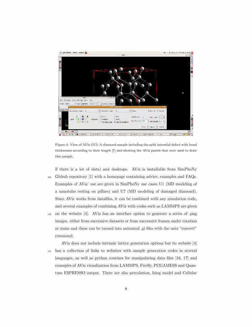
Figure 4: View of AViz GUI: A diamond sample including the split interstial defect with bond

thicknesses according to their length [7] and showing the AViz panels that were used to draw

this sample.

if there is a lot of data) and desktops. AViz is installable from SimPhoNy

Github repository [1] with a homepage containing advice, examples and FAQs.105

Examples of AViz’ use are given in SimPhoNy use cases U1 (MD modeling of

a nanotube resting on pillars) and U7 (MD modeling of damaged diamond).

Since AViz works from datafiles, it can be combined with any simulation code,

and several examples of combining AViz with codes such as LAMMPS are given

on the website [4]. AViz has an interface option to generate a series of .png110

images, either from successive datasets or from successive frames under rotation

or zoom and these can be turned into animated .gi files with the unix “convert”

command.

AViz does not include intrinsic lattice generation options but its website [4]

has a collection of links to websites with sample generation codes in several115

languages, as well as python routines for manipulating data files [16, 17] and

examples of AViz visualization from LAMMPS, Firefly, PCGAMESS and Quan-

tum ESPRESSO output. There are also percolation, Ising model and Cellular

8

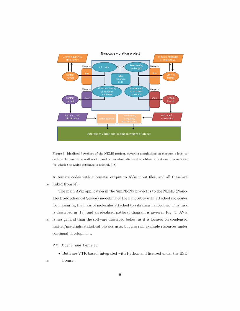
Figure 5: Idealised flowchart of the NEMS project, covering simulations on electronic level to

deduce the nanotube wall width, and on an atomistic level to obtain vibrational frequencies,

for which the width estimate is needed. [18].

Automata codes with automatic output to AViz input files, and all these are

linked from [4].120

The main AViz application in the SimPhoNy project is to the NEMS (Nano-

Electro-Mechanical Sensor) modelling of the nanotubes with attached molecules

for measuring the mass of molecules attached to vibrating nanotubes. This task

is described in [18], and an idealised pathway diagram is given in Fig. 5. AViz

is less general than the software described below, as it is focused on condensed125

matter/materials/statistical physics uses, but has rich example resources under

continual development.

2.2. Mayavi and Paraview

• Both are VTK based, integrated with Python and licensed under the BSD

license.130

9

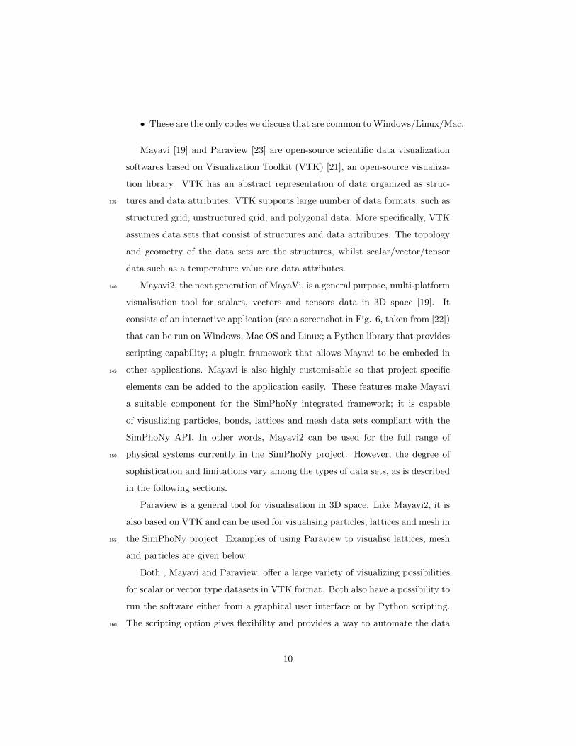
• These are the only codes we discuss that are common to Windows/Linux/Mac.

Mayavi [19] and Paraview [23] are open-source scientific data visualization

softwares based on Visualization Toolkit (VTK) [21], an open-source visualiza-

tion library. VTK has an abstract representation of data organized as struc-

tures and data attributes: VTK supports large number of data formats, such as135

structured grid, unstructured grid, and polygonal data. More specifically, VTK

assumes data sets that consist of structures and data attributes. The topology

and geometry of the data sets are the structures, whilst scalar/vector/tensor

data such as a temperature value are data attributes.

Mayavi2, the next generation of MayaVi, is a general purpose, multi-platform140

visualisation tool for scalars, vectors and tensors data in 3D space [19]. It

consists of an interactive application (see a screenshot in Fig. 6, taken from [22])

that can be run on Windows, Mac OS and Linux; a Python library that provides

scripting capability; a plugin framework that allows Mayavi to be embeded in

other applications. Mayavi is also highly customisable so that project specific145

elements can be added to the application easily. These features make Mayavi

a suitable component for the SimPhoNy integrated framework; it is capable

of visualizing particles, bonds, lattices and mesh data sets compliant with the

SimPhoNy API. In other words, Mayavi2 can be used for the full range of

physical systems currently in the SimPhoNy project. However, the degree of150

sophistication and limitations vary among the types of data sets, as is described

in the following sections.

Paraview is a general tool for visualisation in 3D space. Like Mayavi2, it is

also based on VTK and can be used for visualising particles, lattices and mesh in

the SimPhoNy project. Examples of using Paraview to visualise lattices, mesh155

and particles are given below.

Both , Mayavi and Paraview, offer a large variety of visualizing possibilities

for scalar or vector type datasets in VTK format. Both also have a possibility to

run the software either from a graphical user interface or by Python scripting.

The scripting option gives flexibility and provides a way to automate the data160

10

Figure 6: This is one of many images from the scipy cookbook [22], and shows a Mayavi

interface.

visualization of large datasets like time series, and this way render for example

frames for videos.

2.3. nCAD and nFLUID

This pair of CAD (Computer Aided Design) systems is windows based and

commercial and they share many features. nCAD (nanotechnology CAD) con-165

nects 3D Computer-Aided Design (CAD) programs and atomic visualization and

is fully developed by Sgenia. nCAD provides an user-friendly and common en-

vironment for pre-processing, modelling, visualization and post-processing com-

plex systems at the nano/atomic scale for any dimensionality with a powerful

GUI. It can work with assemblies of pieces designed in traditional CAD soft-170

ware, both importing the geometry from any CAD or plugging-in to Solidworks

[28]. Furthermore, nCAD provides the possibility to design simple pieces in

11

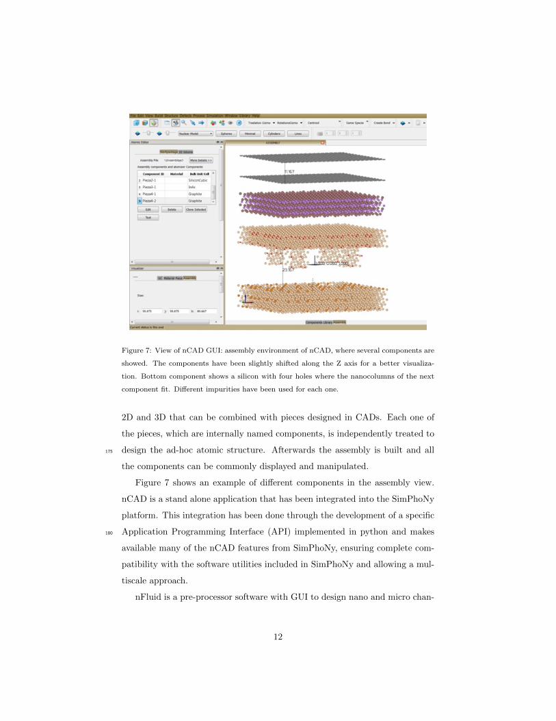
Figure 7: View of nCAD GUI: assembly environment of nCAD, where several components are

showed. The components have been slightly shifted along the Z axis for a better visualiza-

tion. Bottom component shows a silicon with four holes where the nanocolumns of the next

component fit. Different impurities have been used for each one.

2D and 3D that can be combined with pieces designed in CADs. Each one of

the pieces, which are internally named components, is independently treated to

design the ad-hoc atomic structure. Afterwards the assembly is built and all175

the components can be commonly displayed and manipulated.

Figure 7 shows an example of different components in the assembly view.

nCAD is a stand alone application that has been integrated into the SimPhoNy

platform. This integration has been done through the development of a specific

Application Programming Interface (API) implemented in python and makes180

available many of the nCAD features from SimPhoNy, ensuring complete com-

patibility with the software utilities included in SimPhoNy and allowing a mul-

tiscale approach.

nFluid is a pre-processor software with GUI to design nano and micro chan-

12

nels fully developed by Sgenia. nFluid provides the capability to build complex185

and multi-connected channels with any geometrical section (cylindrical and pris-

matic) and ad-hoc shape in a simple and intuitive manner. The software includes

an automatic solver for the geometry that calculates the resulted assembly and

identifies possible errors introduced by the user. All the features are available

through an API for Python and through a fully functional GUI, which also pro-190

vides visualization features. nFluid is completely integrated in SimPhoNy and

thus fully compatible with other SimPhoNy software.

3. Electronic model-based simulations

3.1. Visualization with AViz

One of the object options in the original AViz is “dots” to enabled a quick195

sample build to check object locations. This possibility has been developed into

an offlabel application to visualize field density and can be used as smoke density

to show electronic density with options for color binning [11] and stereo [12, 13].

In the same style as for the other AViz realizations, the above papers and

the websites linked therein provide clear guidelines for physicists and materials200

scientists to use this approach. In Fig. 8 we show a binned colored hydrogen

atom wavefunction, and the analglyphic stereo electronic density of a nanotube.

Note that the nanotube image has the density dots randomly dilluted toenable

the almost transparent view of the inner parts of the system. An example of this

electronic density visualization in conjunction with Quantum ESPRESSO codes205

is given in use cases U8 and U13 related to DFT modelling of nanotubes. On a

typical LINUX desktop box, several hundred thousand dots can be drawn with

ease. Full instructions for AViz use in combination with Quantum ESPRESSO

are given in [12].

3.2. Visualization with Mayavi210

Electron density functions can be a represented as point scalar data and

visualised using the volume rendering method as shown in Fig. 9. In addition

13

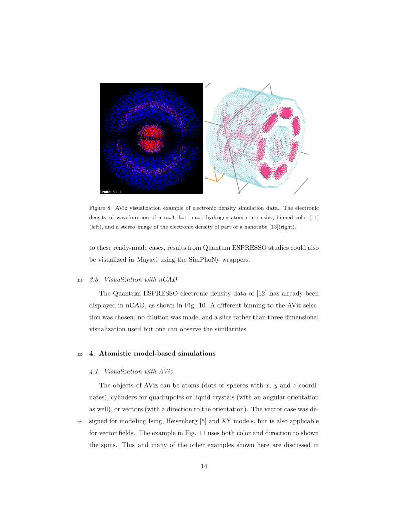
Figure 8: AViz visualization example of electronic density simulation data. The electronic

density of wavefunction of a n=3, l=1, m=1 hydrogen atom state using binned color [11]

(left), and a stereo image of the electronic density of part of a nanotube [13](right).

to these ready-made cases, results from Quantum ESPRESSO studies could also

be visualized in Mayavi using the SimPhoNy wrappers.

3.3. Visualization with nCAD215

The Quantum ESPRESSO electronic density data of [12] has already been

displayed in nCAD, as shown in Fig. 10. A different binning to the AViz selec-

tion was chosen, no dilution was made, and a slice rather than three dimensional

visualization used but one can observe the similarities

4. Atomistic model-based simulations220

4.1. Visualization with AViz

The objects of AViz can be atoms (dots or spheres with x, y and z coordi-

nates), cylinders for quadrupoles or liquid crystals (with an angular orientation

as well), or vectors (with a direction to the orientation). The vector case was de-

signed for modeling Ising, Heisenberg [5] and XY models, but is also applicable225

for vector fields. The example in Fig. 11 uses both color and direction to shown

the spins. This and many of the other examples shown here are discussed in

14

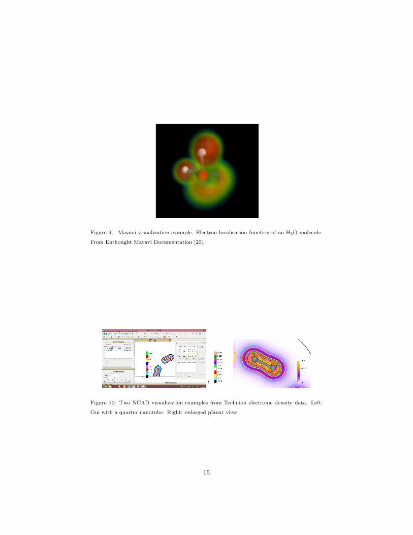
Figure 9: Mayavi visualization example. Electron localisation function of an H2O molecule.

From Enthought Mayavi Documentation [20].

Figure 10: Two NCAD visualization examples from Technion electronic density data. Left:

Gui with a quarter nanotube. Right: enlarged planar view.

15

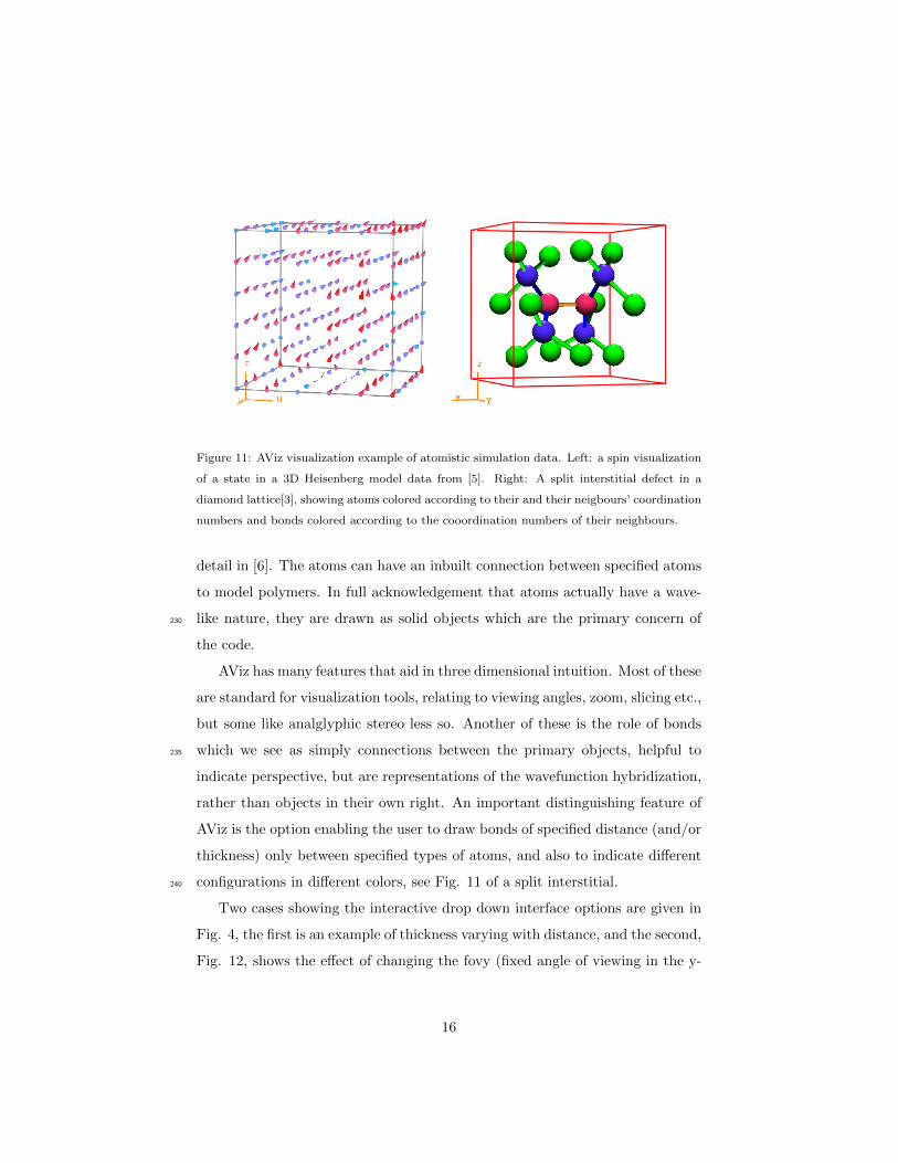
Figure 11: AViz visualization example of atomistic simulation data. Left: a spin visualization

of a state in a 3D Heisenberg model data from [5]. Right: A split interstitial defect in a

diamond lattice[3], showing atoms colored according to their and their neigbours’ coordination

numbers and bonds colored according to the cooordination numbers of their neighbours.

detail in [6]. The atoms can have an inbuilt connection between specified atoms

to model polymers. In full acknowledgement that atoms actually have a wave-

like nature, they are drawn as solid objects which are the primary concern of230

the code.

AViz has many features that aid in three dimensional intuition. Most of these

are standard for visualization tools, relating to viewing angles, zoom, slicing etc.,

but some like analglyphic stereo less so. Another of these is the role of bonds

which we see as simply connections between the primary objects, helpful to235

indicate perspective, but are representations of the wavefunction hybridization,

rather than objects in their own right. An important distinguishing feature of

AViz is the option enabling the user to draw bonds of specified distance (and/or

thickness) only between specified types of atoms, and also to indicate different

configurations in different colors, see Fig. 11 of a split interstitial.240

Two cases showing the interactive drop down interface options are given in

Fig. 4, the first is an example of thickness varying with distance, and the second,

Fig. 12, shows the effect of changing the fovy (fixed angle of viewing in the y-

16

Figure 12: AViz visualization example of atomistic simulation data. An example of fovy

(angle of viewing in the y direction) variation, with perspective at left and a straight-on view

at right, from [7].

Figure 13: AViz visualization example of atomistic simulation data. Left: An example of a

nanotube in a red-cyan stereo view, from [9] Right: An AViz vector field (magnetic field of a

bar magnet) example from an undergraduate course project [10]

direction), both from [7]. The latter case is from a paper about the formation

of diamond membranes [8], showing a graphitized region ready for removal in245

yellow. These possibilities are of paramount importance when studying defects

or crystal interfaces, where interest centers on the disturbed atoms rather than

the translationally invariant ones. This feature was born from frustration with

those chemical visualization packages which drew bonds of specific lengths at

specific angles between atoms of specific types. A recent addition to AViz is an250

analglyphic (red/cyan) stereo feature, [9], which as shown in Fig. 13 further

enhances three dimensional vision.

17

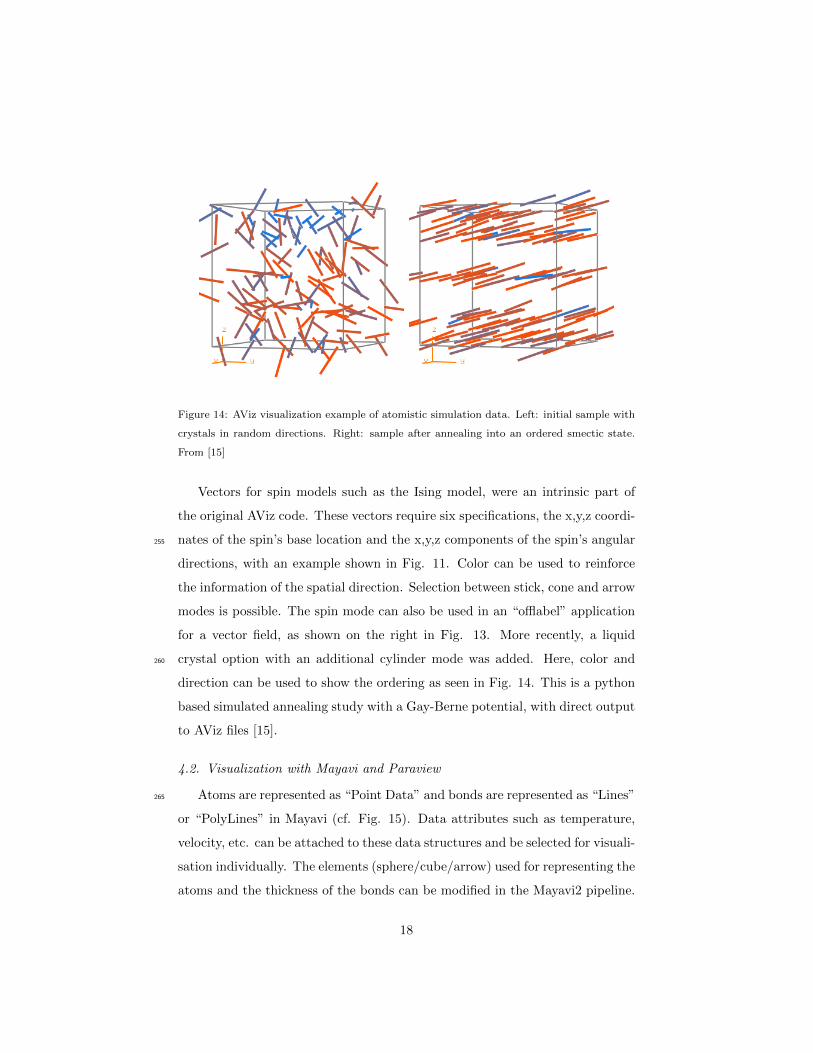
Figure 14: AViz visualization example of atomistic simulation data. Left: initial sample with

crystals in random directions. Right: sample after annealing into an ordered smectic state.

From [15]

Vectors for spin models such as the Ising model, were an intrinsic part of

the original AViz code. These vectors require six specifications, the x,y,z coordi-

nates of the spin’s base location and the x,y,z components of the spin’s angular255

directions, with an example shown in Fig. 11. Color can be used to reinforce

the information of the spatial direction. Selection between stick, cone and arrow

modes is possible. The spin mode can also be used in an “offlabel” application

for a vector field, as shown on the right in Fig. 13. More recently, a liquid

crystal option with an additional cylinder mode was added. Here, color and260

direction can be used to show the ordering as seen in Fig. 14. This is a python

based simulated annealing study with a Gay-Berne potential, with direct output

to AViz files [15].

4.2. Visualization with Mayavi and Paraview

Atoms are represented as “Point Data” and bonds are represented as “Lines”265

or “PolyLines” in Mayavi (cf. Fig. 15). Data attributes such as temperature,

velocity, etc. can be attached to these data structures and be selected for visuali-

sation individually. The elements (sphere/cube/arrow) used for representing the

atoms and the thickness of the bonds can be modified in the Mayavi2 pipeline.

18

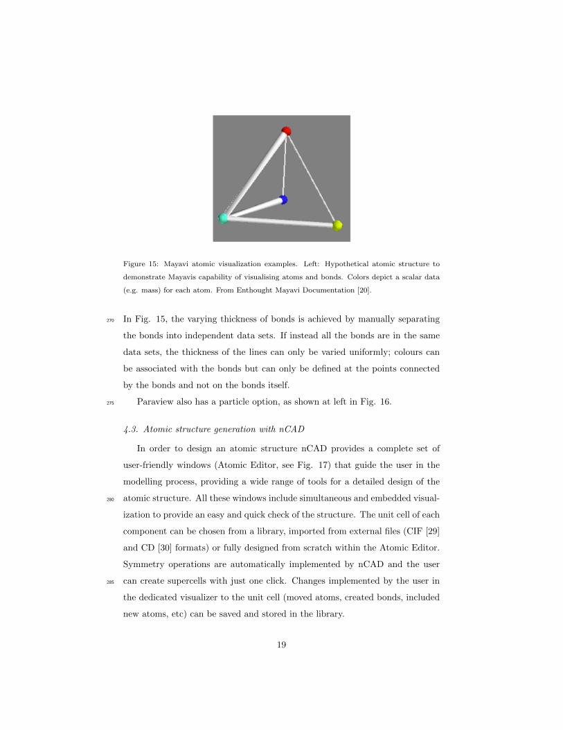
Figure 15: Mayavi atomic visualization examples. Left: Hypothetical atomic structure to

demonstrate Mayavis capability of visualising atoms and bonds. Colors depict a scalar data

(e.g. mass) for each atom. From Enthought Mayavi Documentation [20].

In Fig. 15, the varying thickness of bonds is achieved by manually separating270

the bonds into independent data sets. If instead all the bonds are in the same

data sets, the thickness of the lines can only be varied uniformly; colours can

be associated with the bonds but can only be defined at the points connected

by the bonds and not on the bonds itself.

Paraview also has a particle option, as shown at left in Fig. 16.275

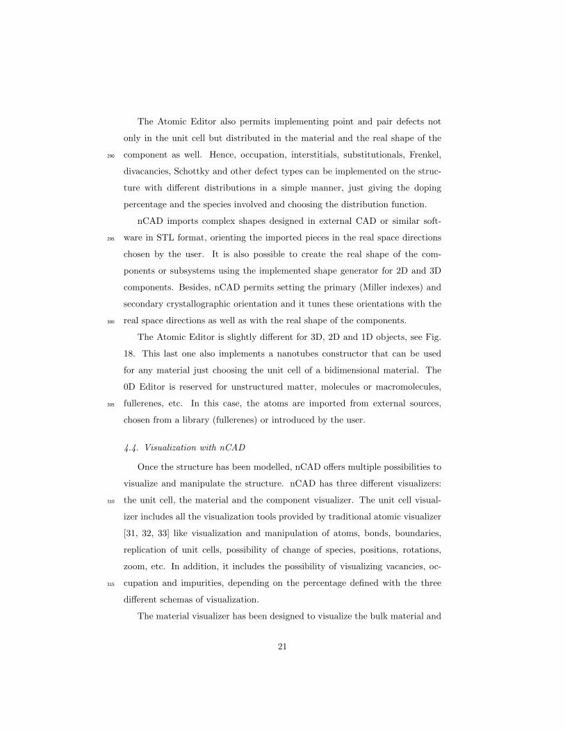
4.3. Atomic structure generation with nCAD

In order to design an atomic structure nCAD provides a complete set of

user-friendly windows (Atomic Editor, see Fig. 17) that guide the user in the

modelling process, providing a wide range of tools for a detailed design of the

atomic structure. All these windows include simultaneous and embedded visual-280

ization to provide an easy and quick check of the structure. The unit cell of each

component can be chosen from a library, imported from external files (CIF [29]

and CD [30] formats) or fully designed from scratch within the Atomic Editor.

Symmetry operations are automatically implemented by nCAD and the user

can create supercells with just one click. Changes implemented by the user in285

the dedicated visualizer to the unit cell (moved atoms, created bonds, included

new atoms, etc) can be saved and stored in the library.

19

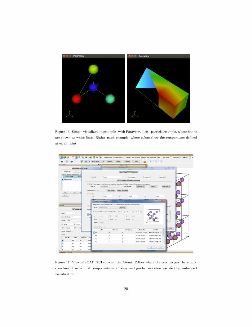
Figure 16: Simple visualization examples with Paraview. Left: particle example, where bonds

are shown as white lines. Right: mesh example, where colors show the temperature defined

at ea ch point.

Figure 17: View of nCAD GUI showing the Atomic Editor where the user designs the atomic

structure of individual components in an easy and guided workflow assisted by embedded

visualization.

20

The Atomic Editor also permits implementing point and pair defects not

only in the unit cell but distributed in the material and the real shape of the

component as well. Hence, occupation, interstitials, substitutionals, Frenkel,290

divacancies, Schottky and other defect types can be implemented on the struc-

ture with different distributions in a simple manner, just giving the doping

percentage and the species involved and choosing the distribution function.

nCAD imports complex shapes designed in external CAD or similar soft-

ware in STL format, orienting the imported pieces in the real space directions295

chosen by the user. It is also possible to create the real shape of the com-

ponents or subsystems using the implemented shape generator for 2D and 3D

components. Besides, nCAD permits setting the primary (Miller indexes) and

secondary crystallographic orientation and it tunes these orientations with the

real space directions as well as with the real shape of the components.300

The Atomic Editor is slightly different for 3D, 2D and 1D objects, see Fig.

18. This last one also implements a nanotubes constructor that can be used

for any material just choosing the unit cell of a bidimensional material. The

0D Editor is reserved for unstructured matter, molecules or macromolecules,

fullerenes, etc. In this case, the atoms are imported from external sources,305

chosen from a library (fullerenes) or introduced by the user.

4.4. Visualization with nCAD

Once the structure has been modelled, nCAD offers multiple possibilities to

visualize and manipulate the structure. nCAD has three different visualizers:

the unit cell, the material and the component visualizer. The unit cell visual-310

izer includes all the visualization tools provided by traditional atomic visualizer

[31, 32, 33] like visualization and manipulation of atoms, bonds, boundaries,

replication of unit cells, possibility of change of species, positions, rotations,

zoom, etc. In addition, it includes the possibility of visualizing vacancies, oc-

cupation and impurities, depending on the percentage defined with the three315

different schemas of visualization.

The material visualizer has been designed to visualize the bulk material and

21

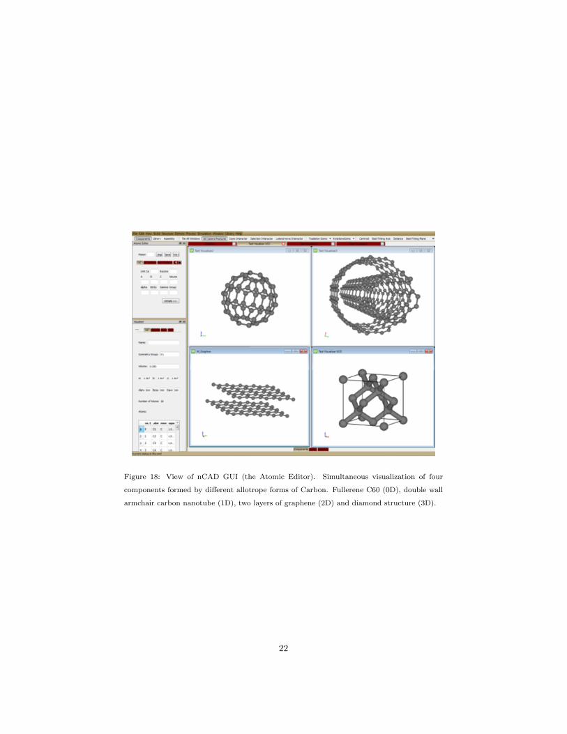
Figure 18: View of nCAD GUI (the Atomic Editor). Simultaneous visualization of four

components formed by different allotrope forms of Carbon. Fullerene C60 (0D), double wall

armchair carbon nanotube (1D), two layers of graphene (2D) and diamond structure (3D).

22

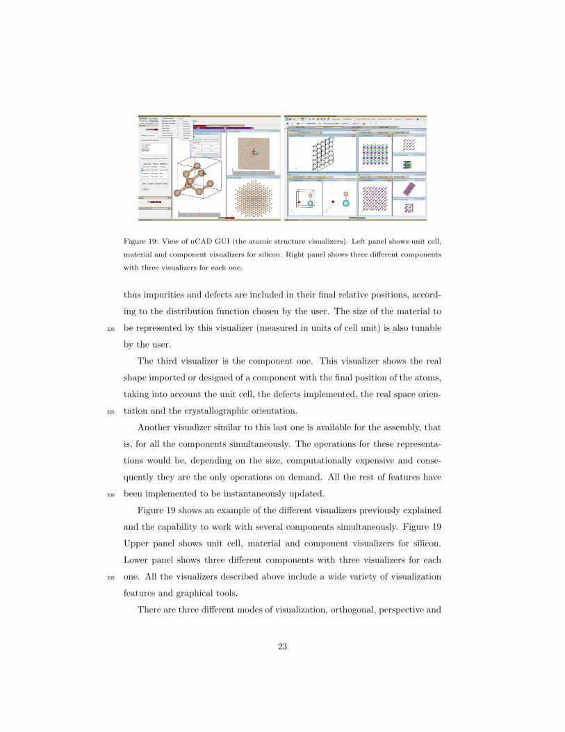
Figure 19: View of nCAD GUI (the atomic structure visualizers). Left panel shows unit cell,

material and component visualizers for silicon. Right panel shows three different components

with three visualizers for each one.

thus impurities and defects are included in their final relative positions, accord-

ing to the distribution function chosen by the user. The size of the material to

be represented by this visualizer (measured in units of cell unit) is also tunable320

by the user.

The third visualizer is the component one. This visualizer shows the real

shape imported or designed of a component with the final position of the atoms,

taking into account the unit cell, the defects implemented, the real space orien-

tation and the crystallographic orientation.325

Another visualizer similar to this last one is available for the assembly, that

is, for all the components simultaneously. The operations for these representa-

tions would be, depending on the size, computationally expensive and conse-

quently they are the only operations on demand. All the rest of features have

been implemented to be instantaneously updated.330

Figure 19 shows an example of the different visualizers previously explained

and the capability to work with several components simultaneously. Figure 19

Upper panel shows unit cell, material and component visualizers for silicon.

Lower panel shows three different components with three visualizers for each

one. All the visualizers described above include a wide variety of visualization335

features and graphical tools.

There are three different modes of visualization, orthogonal, perspective and

23

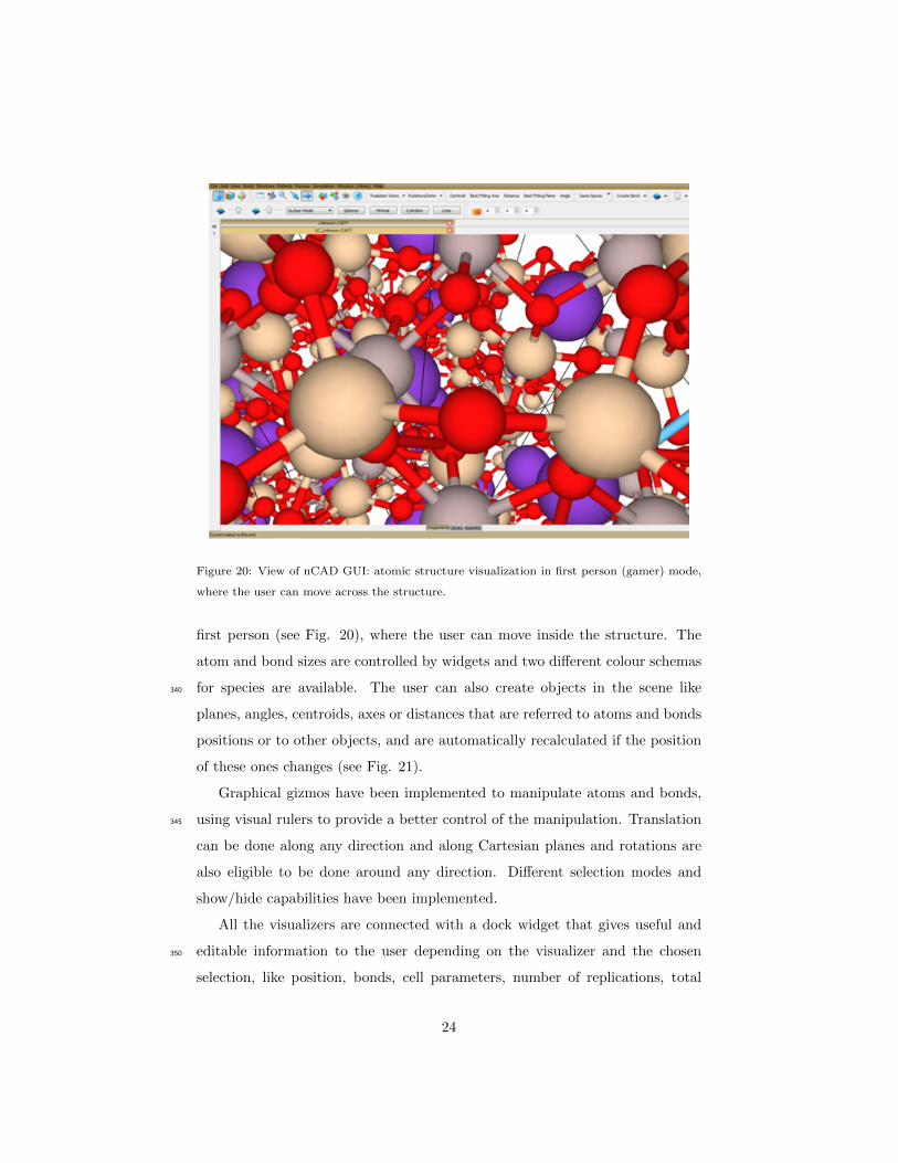
Figure 20: View of nCAD GUI: atomic structure visualization in first person (gamer) mode,

where the user can move across the structure.

first person (see Fig. 20), where the user can move inside the structure. The

atom and bond sizes are controlled by widgets and two different colour schemas

for species are available. The user can also create objects in the scene like340

planes, angles, centroids, axes or distances that are referred to atoms and bonds

positions or to other objects, and are automatically recalculated if the position

of these ones changes (see Fig. 21).

Graphical gizmos have been implemented to manipulate atoms and bonds,

using visual rulers to provide a better control of the manipulation. Translation345

can be done along any direction and along Cartesian planes and rotations are

also eligible to be done around any direction. Different selection modes and

show/hide capabilities have been implemented.

All the visualizers are connected with a dock widget that gives useful and

editable information to the user depending on the visualizer and the chosen350

selection, like position, bonds, cell parameters, number of replications, total

24

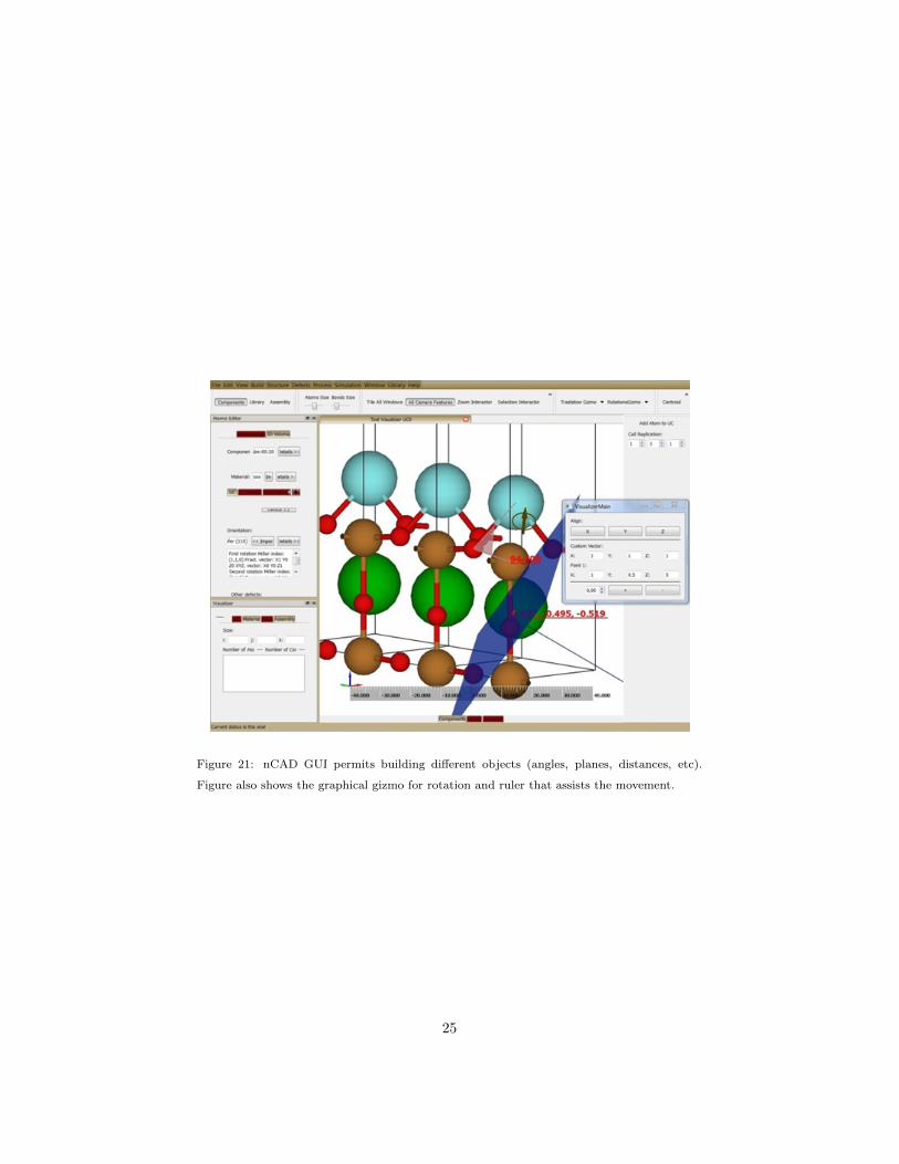
Figure 21: nCAD GUI permits building different objects (angles, planes, distances, etc).

Figure also shows the graphical gizmo for rotation and ruler that assists the movement.

25

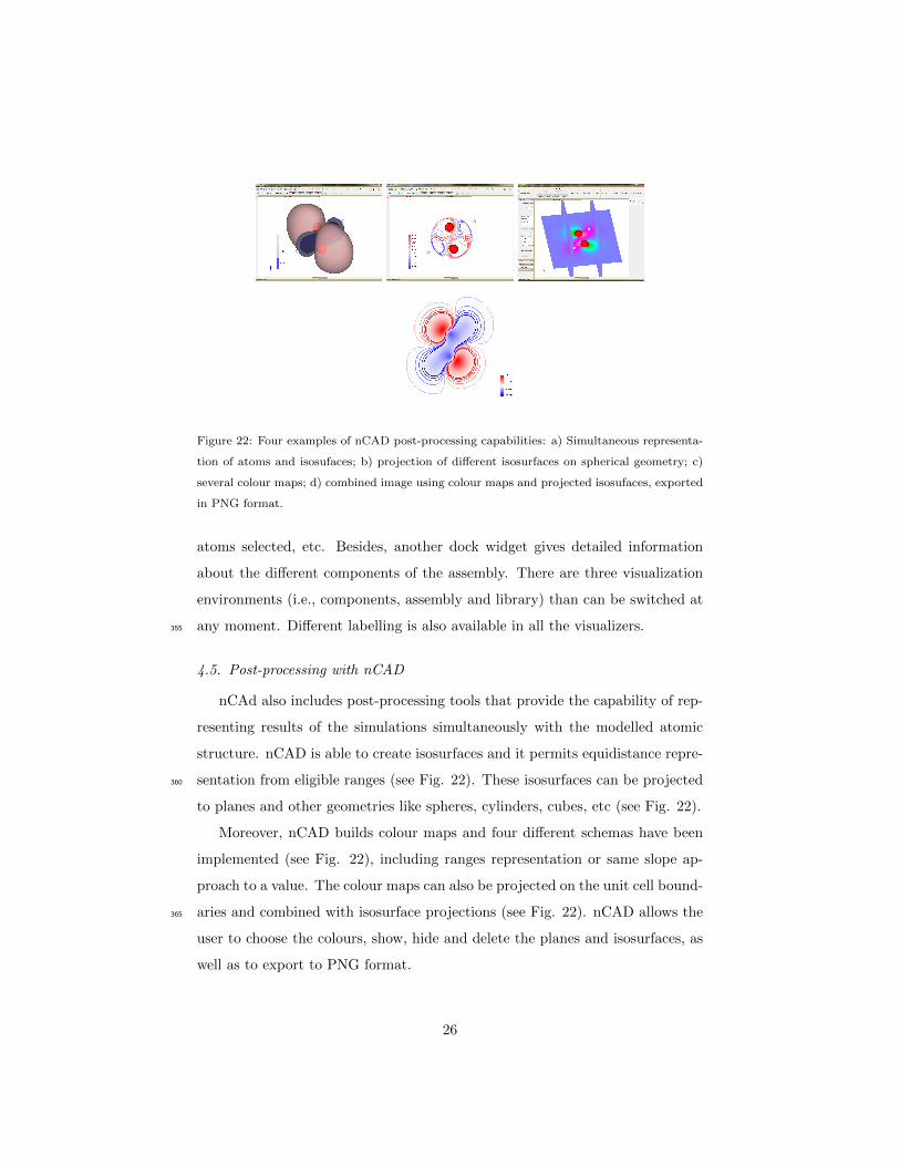
Figure 22: Four examples of nCAD post-processing capabilities: a) Simultaneous representa-

tion of atoms and isosufaces; b) projection of different isosurfaces on spherical geometry; c)

several colour maps; d) combined image using colour maps and projected isosufaces, exported

in PNG format.

atoms selected, etc. Besides, another dock widget gives detailed information

about the different components of the assembly. There are three visualization

environments (i.e., components, assembly and library) than can be switched at

any moment. Different labelling is also available in all the visualizers.355

4.5. Post-processing with nCAD

nCAd also includes post-processing tools that provide the capability of rep-

resenting results of the simulations simultaneously with the modelled atomic

structure. nCAD is able to create isosurfaces and it permits equidistance repre-

sentation from eligible ranges (see Fig. 22). These isosurfaces can be projected360

to planes and other geometries like spheres, cylinders, cubes, etc (see Fig. 22).

Moreover, nCAD builds colour maps and four different schemas have been

implemented (see Fig. 22), including ranges representation or same slope ap-

proach to a value. The colour maps can also be projected on the unit cell bound-

aries and combined with isosurface projections (see Fig. 22). nCAD allows the365

user to choose the colours, show, hide and delete the planes and isosurfaces, as

well as to export to PNG format.

26

Figure 23: Mayavi and Paraview visualization examples of continuum-model based simulation

data. Left: Visualization of a simulated pressured-driven flow in a tube (simulated with the

Kratos CFD engine) using Mayavi; colors on the tube show the pressure values and vectors

(and its color) show the velocity (and speed). Right: Cubic lattice example visualised using

Paraview.

5. Continuum model-based simulations

5.1. Visualization with Mayavi and Paraview

Computational modelling of continuum dynamics generally require utiliza-370

tion of mesh datasets containing points which are connected to form edges,

faces and cells. These types of data are represented using the most general

VTK dataset called “UnstructuredGrid”. Currently, in the SimPhoNy wrap-

pers for Mayavi and Paraview, all mesh datasets are represented using the “Un-

structuredGrid”. Future plans involve using “PolyData” for mesh datasets that375

only contain points for enhanced efficiency. An example using the Kratos CFD

engine[24] to simulate pressure-driven flow in a tube is shown in Fig. 23 at left:

colors on the tube show the pressure values and vectors (and its color) show the

velocity (and speed).

Similar to particles, lattice nodes are also represented using point data. The380

topology and geometry of the nodes, however, may be represented using differ-

ent VTK datasets depending on the type of lattices. For cubic, tetragonal, and

27

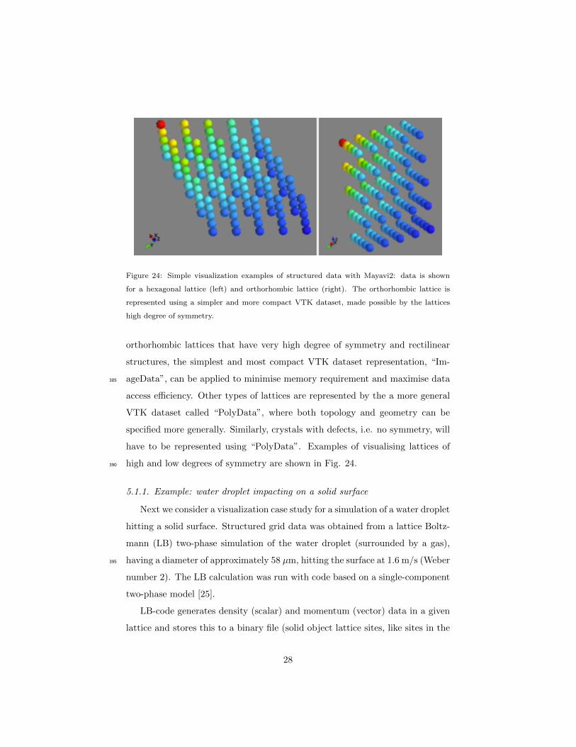
Figure 24: Simple visualization examples of structured data with Mayavi2: data is shown

for a hexagonal lattice (left) and orthorhombic lattice (right). The orthorhombic lattice is

represented using a simpler and more compact VTK dataset, made possible by the lattices

high degree of symmetry.

orthorhombic lattices that have very high degree of symmetry and rectilinear

structures, the simplest and most compact VTK dataset representation, “Im-

ageData”, can be applied to minimise memory requirement and maximise data385

access efficiency. Other types of lattices are represented by the a more general

VTK dataset called “PolyData”, where both topology and geometry can be

specified more generally. Similarly, crystals with defects, i.e. no symmetry, will

have to be represented using “PolyData”. Examples of visualising lattices of

high and low degrees of symmetry are shown in Fig. 24.390

5.1.1. Example: water droplet impacting on a solid surface

Next we consider a visualization case study for a simulation of a water droplet

hitting a solid surface. Structured grid data was obtained from a lattice Boltz-

mann (LB) two-phase simulation of the water droplet (surrounded by a gas),

having a diameter of approximately 58 µm, hitting the surface at 1.6 m/s (Weber395

number 2). The LB calculation was run with code based on a single-component

two-phase model [25].

LB-code generates density (scalar) and momentum (vector) data in a given

lattice and stores this to a binary file (solid object lattice sites, like sites in the

28

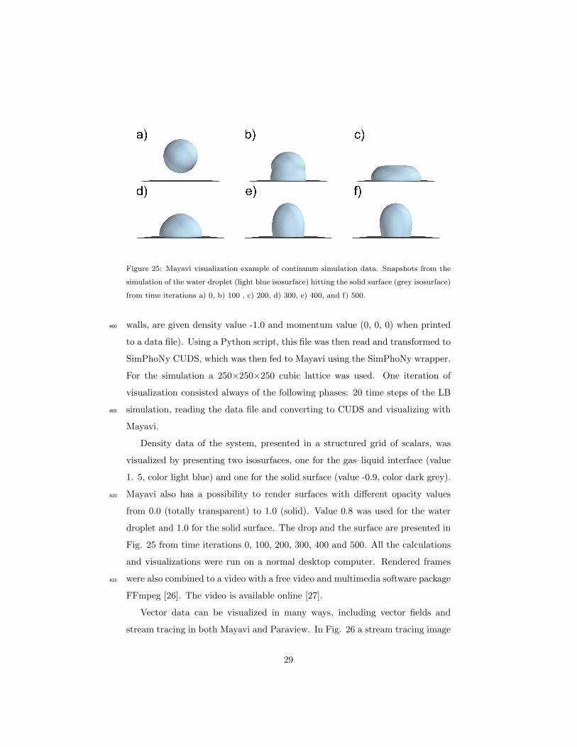
Figure 25: Mayavi visualization example of continuum simulation data. Snapshots from the

simulation of the water droplet (light blue isosurface) hitting the solid surface (grey isosurface)

from time iterations a) 0, b) 100 , c) 200, d) 300, e) 400, and f) 500.

walls, are given density value -1.0 and momentum value (0, 0, 0) when printed400

to a data file). Using a Python script, this file was then read and transformed to

SimPhoNy CUDS, which was then fed to Mayavi using the SimPhoNy wrapper.

For the simulation a 250×250×250 cubic lattice was used. One iteration of

visualization consisted always of the following phases: 20 time steps of the LB

simulation, reading the data file and converting to CUDS and visualizing with405

Mayavi.

Density data of the system, presented in a structured grid of scalars, was

visualized by presenting two isosurfaces, one for the gas–liquid interface (value

1. 5, color light blue) and one for the solid surface (value -0.9, color dark grey).

Mayavi also has a possibility to render surfaces with different opacity values410

from 0.0 (totally transparent) to 1.0 (solid). Value 0.8 was used for the water

droplet and 1.0 for the solid surface. The drop and the surface are presented in

Fig. 25 from time iterations 0, 100, 200, 300, 400 and 500. All the calculations

and visualizations were run on a normal desktop computer. Rendered frames

were also combined to a video with a free video and multimedia software package415

FFmpeg [26]. The video is available online [27].

Vector data can be visualized in many ways, including vector fields and

stream tracing in both Mayavi and Paraview. In Fig. 26 a stream tracing image

29

Figure 26: Paraview visualization example of continuum simulation data. Stream tracing

visualization of the water droplet which has hit the surface and is bouncing back.

from the water droplet (surrounded by a gas) is presented from Paraview. It

has hit the surface and is bouncing back. Geometry was visualized again by the420

isosurface representation and with the same values specified above.

5.2. Geometry generation with nFLUID

nFluid has a powerful and user-friendly Channel Editor where the user can

design the geometry of the channels. For this purpose, predesigned individual

pieces have been developed lending the user the possibility to create any set of425

connected and complex channels, including flow adapters, expansion chambers,

tees and any type of elbow joints. The user just has to care about the general

characteristics of the channel elements under construction, like the radius, the

bending angle of a joint, the flux direction of the channels, etc.

Due to the automatic solver, the new pieces inherit the parameters of the430

channel where they are located, unless the user defines them. With this minimal

information, nFluid creates, connects and adapts the pieces to build the channels

and creates a mesh to define geometrically the designed channels. Besides,

ad-hoc pieces with complex geometry can be also designed just giving several

positions that the channel must fit and follow (see Fig. 27). These pieces435

30

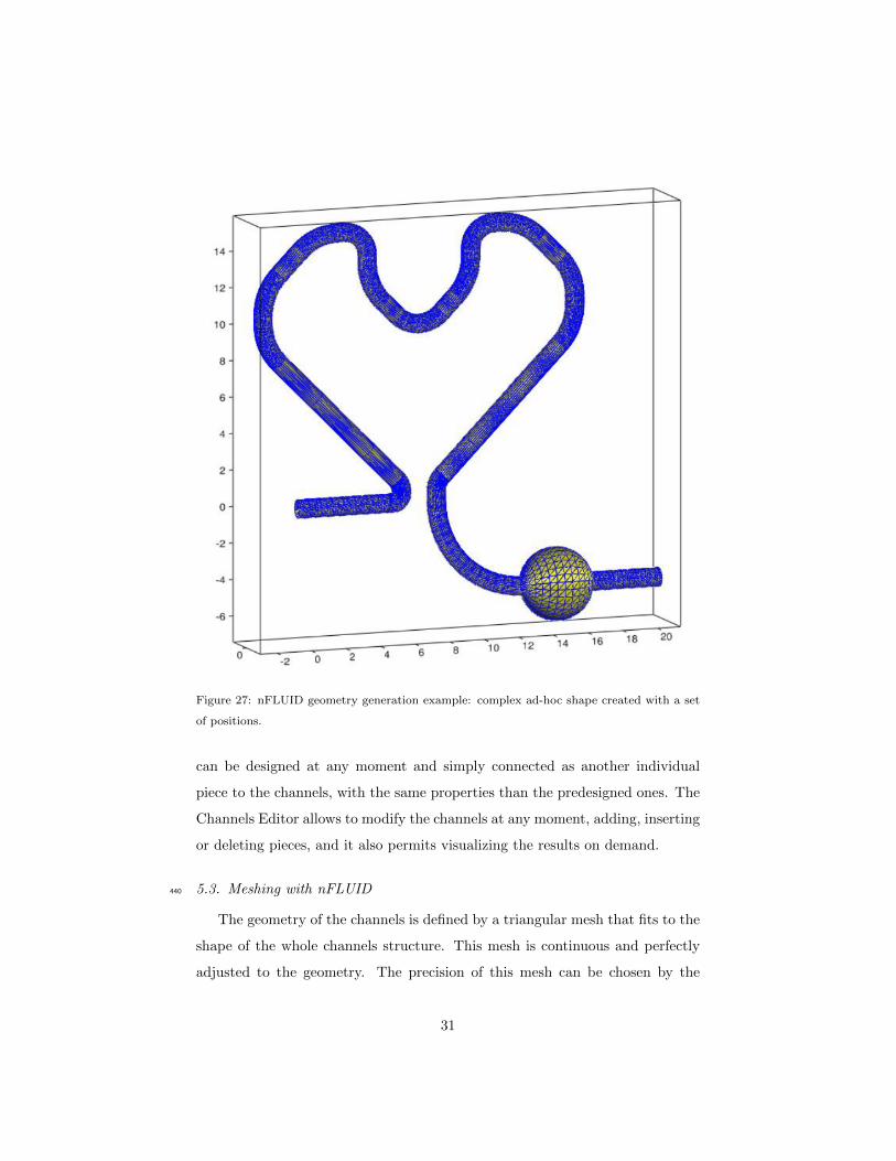
Figure 27: nFLUID geometry generation example: complex ad-hoc shape created with a set

of positions.

can be designed at any moment and simply connected as another individual

piece to the channels, with the same properties than the predesigned ones. The

Channels Editor allows to modify the channels at any moment, adding, inserting

or deleting pieces, and it also permits visualizing the results on demand.

5.3. Meshing with nFLUID440

The geometry of the channels is defined by a triangular mesh that fits to the

shape of the whole channels structure. This mesh is continuous and perfectly

adjusted to the geometry. The precision of this mesh can be chosen by the

31

user and it permits not only improving the definition of the geometry but also

defining a finer mesh useful for subsequent simulation goals. nFluid can also445

construct the negative mesh of the channels, that is, it is able to create a bulk

structure where the channels are perforated inside the bulk. Moreover, it also

allows to choose if the structure, channels and negatives, are closed or open

structures.

nFluid exports the mesh to different formats like STL or SimPhoNy Mesh450

class, and creates projects that can be straightforward imported by OpenFoam

[34]. nFluid also includes an utility to get a text summary of the channels, where

the geometry and a sketch, as well as the main characteristics of the channels

and the parameters of the pieces, are included. GUI All the features described

above are integrated in a GUI that implements a clear and easy workflow.455

Fig. 28 shows the nFluid GUI and the four main parts that the GUI is

divided in are marked in red. The Channel Editor, as it is explained above,

provides to the user a simple manner to design the channel. Two windows

offer the information about the channels: the first one shows the modifiable

list of pieces, while the second one offers a detailed hierarchical sketch of the460

channel. The main window is dedicated to a visualizer that displays the channel

on construction during the design process.

6. Summary

Several different visualization tools integrated and used in SimPhoNy have

been described. There is some overlap, but three very different philosophies are465

observed.

• AViz is motivated by physics research and teaching goals, has a GUI with

extensive drop down menus for and requires individual tailoring for a rich

variety of output. It requires initial datasets, and while it does not have

inbuilt lattice generators, multiple websites with tools and instructions470

are described on its site and in several papers, e.g. [5]. There is also

much web support on its implementation with detailed examples for both

32

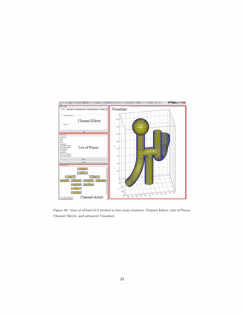
Figure 28: View of nFluid GUI divided in four main windows: Channel Editor, List of Pieces,

Channel Sketch, and advanced Visualizer.

33

HPC and educational uses. Even prior to SimPhoNy, guidance for use

with LAMMPS and Quantum ESPRESSO was published, [12] and during

simPhoNY python wrapper version sfor this have been created. AViz has475

a command line option but is best used with its GUI. There are scripts in

several languages, including python, on some of the websites.

• Mayavi2 and Paraview are probably the most general codes, and have

scripting or interactive options, and one or the other (or either) can be

used for almost every type of vizualization. Again there is a lot of web480

support for their implementation, such as [24]. They have GUI or python

scripting usage choice, [22].

• nCAD and nFLUID are CAD tools, with many possibilities, and can in-

teract with the OpenFoam code (as can Mayavi and Paraview). Their

GUI options are extensive as our selected examples demonstrate.485

To some extent, AViz and nCAD are at extremes, with the former directly

tied to electronic/atomistic/statistical physics simulation codes and the latter

capable of generating complicated model systems. We presented nCAD ex-

amples with Technion Qantum ESPRESSO data, as shown in Figs. 8 10 and

although not discussed explicitly above the AViz nanotube datafile generation490

website and algorithms [16] have been connected to the nCAD GUI. Mayavi2

and Paraview are more “all purpose”, but there is web information on their

integration with many well-known codes, for example see [22].

In Table 1 some of the differences are summarized.

Acknowledgements: These results are part of the SimPhoNy project.495

SimPhoNy is an FP7 program of the European Commission (FP7-NMP-2013-

SMALL-7) with grant number 604005. In addition, support from the program

Plan Avanza from the Ministerio de Industria, Energıa y Comercio from Go-

bierno de Espana, grant number TSI-020100-2011-300, was used for case of

nCAD.500

34

Table 1: Comparison of various vizualization tools considered.

AViz AViz nCAD nFLUID mayavi paraview

(at.) (el.)

Atomistic scale yes no yes no yes yes

Electronic scale no yes yes no yes yes

Continuum scale no no no yes yes yes

Microsoft no no yes yes yes yes

Mac no no no no yes yes

LINUX yes yes no yes yes yes

OpenGL/Mesa yes yes yes yes yes yes

Stereo yes yes no no yes yes

References

[1] The SimPhoNy project: http://www.simphony-project.eu/; the SimPhoNy

GitHub repository: https://github.com/simphony

[2] J. Adler, A. Hashibon, N. Schreiber, A. Sorkin, S. Sorkin and G. Wag-

ner, “Visualization of MD and MC Simulations for Atomistic Modeling“,505

Computer Physics Communications, (2002) 147, p. 665-9.

[3] J. Adler, A Column for the Simulations section, edited by D. Stauffer in

Computers in Science and Engineering, “Visualization in Atomistic and

Spin Simulations“, (2003) Computers in Science and Engineering, 5, p.

61-65.510

[4] AViz website: http://phony1.technion.ac.il/∼aviz

[5] R. Hihinashvilli, J. Adler, S.H. Tsai and D.P. Landau, “Visualization of

vector spin configurations”, for “Recent Developments in Computer Sim-

ulation Studies in Condensed Matter Physics, XVI”, (2004) edited by D.

Landau, S. P. Lewis and B. Schuttler.515

35

[6] A set of AViz examples with datafiles and instructions:

http://phony1.technion.ac.il/∼phr76ja/plugfest

[7] J. Adler, Y. Koenka and A. Silverman, “Adventures in carbon visualization

with AViz“, (2011) Physics Procedia, 15, 7-16.

[8] Silverman A, Adler J and Kalish R 2011 “Diamond membrane surface af-520

ter ion implantation induced graphitization for graphite removal:molecular

dynamics simulation” Phys. Rev. B 83 155410

[9] D. Peled, A. Silverman and J. Adler “3D visualization of atomistic simula-

tions on every desktop“, (2013) IOP Conference Series, 454, p. 012076.

[10] Class project comparing simulated magnetic field and iron filing patterns:525

http://phelafel.technion.ac.il/∼anatoly

[11] Joan Adler, J. Fox, R. Kalish, T. Mutat, A. Sorkin and E. Warszawski “The

essential role of visualization for modeling nanotubes and nanodiamond“,

(2007) Computer Physics Communications, 177, p. 19-20.

[12] Bastien Grosso, Valentino R. Cooper, Polina Pine, Adham Hashibon, Yu-530

val Yaish and Joan Adler, “Visualization of electronic density“ , (2015)

Computer Physics Communications, 195, p. 1-13.

[13] Joan Adler, , Omri Adler, Meytal Kreif, Or Cohen, Bastien Grosso Adham

Hashibon, Valentino R. Cooper, “Mini-review of Electron Density Visual-

ization“ (2015) Physics Procedia, 68, p. 26.535

[14] Adler J, Fox J, Kalish R, Mutat T, Sorkin A and Warszawski E 2007

”The essential role of visualization for modeling nanotubes and nanodia-

mond”Computer Physics Communications 177 pp 19-20

[15] J. Adler, Hila Glanz and Nadir Izrael,“A Rosetta stone” for AViz” Physics

Procedia, 57c , pp2-6, (2014)540

[16] D. Mazvovsky, G. Halioua and Joan Adler, “The role of projects in (Com-

putational) Physics Education”, Physics Procedia, 2012, Vol 34, p 1-5.

36

[17] Class project presenting visualizations of lattice defects:

http://bananauskha.github.io/aviz/index.html

[18] J. Adler and O. Adler, in preparation and O. Adler, M.Sc. thesis, Technion545

2016.

[19] P. Ramachandran and G. Varoquaux, Mayavi: 3D visualization of scientific

data, (2011) IEEE Computing in Science and Engineering 13(2), pp 40–51

[20] Enthought, “Chemistry example.” (n.d.). Retrieved January 27, 2016, from

http://docs.enthought.com/mayavi/mayavi/auto/example chemistry.html550

[21] W. Schroeder, K. Martin, and B. Lorensen, The visualization toolkit: An

object-oriented approach to 3D graphics, Kitware (Clifton Park, NY, USA),

2006, ISBN 978-1930934191.

[22] http://scipy-cookbook.readthedocs.io

[23] U. Ayachit, The ParaView Guide: A Parallel Visualization Application,555

Kitware (Clifton Park, NY, USA), 2015, ISBN 978-1930934306.

[24] Kratos: A framework for building multi-disciplinary finite element pro-

grams, CIMNE (Barcelona, Spain), http://www.cimne.com/kratos/

[25] P. Yuan and L. Schaefer, Equations of state in a lattice Boltzmann model,

Physics of Fluids, 18(4), 2006560

[26] FFmpeg: A complete, cross-platform solution to record, convert and stream

audio and video, http://www.ffmpeg.org/, accessed: 2016-02-04

[27] online

[28] SolidWorks (https://www.solidworks.com/) by Dassault Systmes

[29] S.R. Hall, F. H. Allen, I. D. Browns The Crystallographic Information565

File (CIF): a New Standard Archive File for Crystallography, Acta Cryst.

(1991). A47, 665-685

37

[30] nCAD propietary format

[31] MaterialsStudio / Biovia by Accelrys of Dassault Systmes

[32] CrystalMaker by CrystalMaker Software Limited570

[33] K. Momma and F. Izumi. VESTA 3 for three-dimensional visualization of

crystal, volumetric and morphology data J. Appl. Crystallogr. (2011), 44,

1272-1276.

[34] OpenFoam by OpenCFD Ltd. H. G. Weller, G. Tabor, H. Jasak, C. Fureby,

A tensorial approach to computational continuum mechanics using object-575

oriented techniques, Comp. Physc. (1998), 12, 620.

38