Visual Servoing on Unknown Objects

Design and implementation of a working system

J A V I E R G R A T A L

Master of Science Thesis Stockholm, Sweden 2012

Visual Servoing on Unknown Objects

Design and implementation of a working system

J A V I E R G R A T A L

DD221X, Master’s Thesis in Computer Science (30 ECTS credits) Degree Progr. in Information and Communication Technology 270 credits Royal Institute of Technology year 2012 Supervisor at CSC was Danica Kragic Examiner was Danica Kragic TRITA-CSC-E 2012:013 ISRN-KTH/CSC/E--12/013--SE ISSN-1653-5715 Royal Institute of Technology School of Computer Science and Communication KTH CSC SE-100 44 Stockholm, Sweden URL: www.kth.se/csc

AbstractThis thesis presents a system where different componentsare integrated to grasp an unknown object. Some of thesecomponents are based on existing work, while others havebeen specifically designed or implemented. One of the com-mon denominators of most of these components is that theymake use of visual servoing techniques. Visual servoing hasbeen traditionally used in applications where the object tobe servoed is known to the robot. Here, these techniquesare used to bring the manipulator towards the object, butalso as a helper tool for calibration and, in what is knownas virtual visual servoing, as a method for pose estimation.

Contents

1 Introduction 1

2 Problem Formulation 32.1 Grasping Pipeline . . . . . . . . . . . . . . . . . . . . . . . . . . . . . 32.2 Error Formalisation . . . . . . . . . . . . . . . . . . . . . . . . . . . 3

2.2.1 Stereo Calibration Error . . . . . . . . . . . . . . . . . . . . . 52.2.2 Positioning Error of the Active Head . . . . . . . . . . . . . . 52.2.3 Positioning Error of the Cameras with Respect to the Arm . 7

3 Related Work 93.1 Closed-Loop Control in Robotic Grasping . . . . . . . . . . . . . . . 93.2 Calibration Methods . . . . . . . . . . . . . . . . . . . . . . . . . . . 103.3 Visual and Virtual Visual Servoing . . . . . . . . . . . . . . . . . . . 10

4 The Proposed System 134.1 Vision System for Constructing the Scene Model . . . . . . . . . . . 144.2 Grasp and Motion Planning . . . . . . . . . . . . . . . . . . . . . . . 144.3 Object Localisation in Different Viewing Frames . . . . . . . . . . . 154.4 Offline Calibration Process . . . . . . . . . . . . . . . . . . . . . . . 16

4.4.1 Stereo Calibration . . . . . . . . . . . . . . . . . . . . . . . . 164.4.2 Head-Eye Calibration . . . . . . . . . . . . . . . . . . . . . . 18

4.5 Virtual Visual Servoing . . . . . . . . . . . . . . . . . . . . . . . . . 214.5.1 Virtual image generation . . . . . . . . . . . . . . . . . . . . 224.5.2 Features . . . . . . . . . . . . . . . . . . . . . . . . . . . . . . 234.5.3 Pose correction . . . . . . . . . . . . . . . . . . . . . . . . . . 234.5.4 Estimation of the jacobian . . . . . . . . . . . . . . . . . . . . 25

4.6 Object grasping . . . . . . . . . . . . . . . . . . . . . . . . . . . . . . 25

5 Experiments 275.1 Robustness of Virtual Visual Servoing . . . . . . . . . . . . . . . . . 275.2 Qualitative Experiments on the Real System . . . . . . . . . . . . . 29

6 Conclusions 33

Bibliography 35

Chapter 1

Introduction

Object grasping and manipulation is one of the fields in robotics that has receivedmost attention lately, but it remains as an open problem. Many of the existingapproaches assume that the object to be manipulated is known beforehand, or atleast that it bears some resemblance to a known object. In these cases, experiencecan be used for grasp synthesis. This is sufficient for most current industrial ap-plications, where tasks consist of the precise and repetitive manipulation of a smallset of objects in a controlled environment. However, before the widespread use ofrobots is possible in other kind of environments, such as for domestic applications,it is necessary to develop systems that can manipulate unknown objects and dealwith the uncertainties that arise from working in a less restricted environment.

The first step towards succesful manipulation of an object consists of graspingthe object. This task involves a whole set of processing steps performed prior tothe actual picking up of an object. Each of these processes represents a potentialsource of inaccuracies which makes it really difficult to succeed unless the errorsare neutralized. As will be shown in this thesis, visual servoing can be used to helpdeal with these errors. The principle of visual servoing is simple: some features (e.g.points, lines or distances) are detected in images (usually obtained in real time fromcameras) and their value is compared with some desired value for these features.Then, movements are performed in order to reduce the discrepancy between theactual and the desired values.

Visual Servoing can help us overcome two kinds of errors in our system. First,the errors coming from the inaccuracies in the hardware calibration, known as sys-tematic or offline errors. Head-eye calibration errors will make us believe that weare looking to a different place; Hand-eye calibration errors make our estimation onwhere is the hand in visual space erroneous; finally, stereo calibration errors makesthe image depth computation inaccurate. The combination of all these errors leadsto inaccuracy in the estimation of the object and manipulator poses and also toa lack of a global coordinate system which consistent through head movements.Therefore the interaction of our robot with the environment is impossible unlessthose errors are corrected. However, these errors can be minimized offline, and we

1

CHAPTER 1. INTRODUCTION

will show how visual servoing can help us to obtain more accurate calibration forour hardware.

The second error type are random or online errors. These errors include, amongothers, limitations in the repeatability of the hardware (due to motor encodersinaccuracies the perceived joint configuration may not correspond to the actualone), dynamic inaccuracies of the motors, image noise and errors in other visualprocesses. These errors can not be corrected offline, so we should neutralize themwhile executing the grasps. This thesis will show how the localization of the roboticarm can be refined in this way, as well as how to bring its end effector to the desiredgrasping point.

The system described in this thesis uses Visual Servoing (VS) at different stagesin the grasping pipeline to correct both of these types of errors. It presents a newmethod that applies VS for the automatic calibration of the hardware. It alsofollows the classical approach of applying VS for aligning the robot hand with theobject prior to grasping it [Kragic and Christensen, 2001]. This requires trackingof the manipulator pose relative to the camera. Instead of the common approachof putting markers on the robot hand, a model based tracking system is used. Thisis achieved through what is known as Virtual Visual Servoing (VVS) in which thesystematic and random errors are compensated for during the grasping procedure.An additional contribution is the generalisation of VVS to complete CAD modelsinstead of using simplified object models specfically designed for the application.

The remainder of this thesis is organised as follows. Chapter 2 formalises thesystematic and random errors inherent to the different parts of the robotic system.In Chapter 3, related work in the area of offline calibration as well as closed-loopcontrol is presented. The method used in the system is described in detail in Chap-ter 4. The performance of some of its parts is analysed quantitatively on syntheticdata and the whole system is evaluated qualitatively on our robotic platform. Theresults of these experiments are presented in Chapter 5.

2

Chapter 2

Problem Formulation

Object grasping in real world scenarios requires a set of steps to be performed priorto the actual manipulation of an object. A general outline of the grasping pipelineis provided in Figure 2.2. The hardware components of the system as shown inFigure 2.1 are (i) the Armar III robotic head [Asfour et al., 2008] equipped withtwo stereo camera pairs (wide-angle for peripheral vision and narrow-angle for fovealvision), (ii) the 6 DoF Kuka arm KR5 sixx R850 [KUKA, Last Visited Dec’10] and(iii) the Schunk Dexterous Hand 2.0 (SDH) [SCHUNK, Last visited Dec’10].

2.1 Grasping Pipeline

The main pre-requisite for a robot to perform a pick-and-place task is to havean understanding of the 3D environment it is acting in. In this pipeline, sceneconstruction is performed by using the active head for visual exploration and stereoreconstruction as described in detail in the previous work [Gratal et al., 2010]. Theresulting point cloud is segmented into object hypotheses and background.

The scene model then consists of the arm and the active head positioned relativeto each other based on the offline calibration as described in Section 4.4. Further-more, a table plane is detected and the online detected object hypotheses are placedon it.

Grasp inference is then performed on each hypothesis. For some given graspcandidates, a collision-free arm trajectory is planned in the scene model and appliedto the object hypothesis with the real arm.

2.2 Error Formalisation

The aforementioned grasping pipeline relies on the assumption that all the parame-ters of the system are perfectly known. This includes internal and external cameraparameters as well as the pose of the head, arm and hand in a globally consistentcoordinate frame.

3

CHAPTER 2. PROBLEM FORMULATION

lower pitch

yaw

roll

Head Origin

upper pitch

eye pitch

left

eyeyaw

right

eyeyaw

Figure 2.1. Hardware Components in the Grasping Pipeline. 2.1(a) Armar IIIActive Head with 7 DoF. 2.1(b) The Kinematic Chain of the Active Head. Theupper pitch is kept static. Right and left eye yaw are actuated during fixation andthereby change the vergence angle and the epipolar geometry. All the other jointsare used for gaze shifts. 2.1(c) Kuka Arm with 6 DoF and Schunk Dexterous Hand2.0 (SDH) with 7 DoF.

Visual SceneConstruction

Images

Control Signals

Grasp Planning

Motion Planning

Target Hand Pose

Control Signals

Scene Model

Segmented 3D Point Cloud

Object Hypotheses

3D Scene

Figure 2.2. Our Open-Loop Grasping Pipeline.

4

2.2. ERROR FORMALISATION

In reality however two different types of errors are inherent to the system. Onecontains the systematic errors that are repeatable and arise from inaccurate cali-bration or inaccurate kinematic models. The other group comprises random errorsoriginating from noise in the motor encoders or in the camera. These errors prop-agate and deteriorate the relative alignment between hand and object. The mostreliable component of the system is the Kuka arm that has a repeatability of lessthan 0.03 mm [KUKA, Last Visited Dec’10]. In the following, the different errorsources are analysed in more detail.

2.2.1 Stereo Calibration Error

Given a set of 3D points QW =[xW yW zW

]Tin the world reference frame W

and their corresponding pixel coordinates P =[u v 1

]Tin the image, the internal

parameters C and external parameters [RCW |tC

W ] can be determined for all camerasC in the vision system. This is done through standard methods by exploiting thefollowing relationship between QW and P :

wP =

wuwvw

= CPC with PC =

zC

yC

zC

= RCW

[PW − tC

W

](2.1)

Once we have these parameters for the left camera L and right camera R, the epipo-lar geometry as defined by the essential matrix E = RR

L [tRL ]× can be determined.

Here tRL defines the baseline and RR

L the rotation between the left and right camerasystem.

The calibration method, which uses the arm as the world reference frame, willbe described in Chapter 4.4. The average reprojection error obtained with thismethod in the hardware described is 0.1 pixels. Since peripheral and foveal camerasare calibrated simultaneously, it is also possible to calculate the transformationbetween them as part of the same process.

In addition to the systematic error in the camera parameters, other effects suchas camera noise and specularities lead to random errors in the stereo matching.

2.2.2 Positioning Error of the Active HeadThe robot head is used to actively explore the environment through gaze shiftsand fixation on objects. This involves dynamically changing the epipolar geometrybetween the left and right camera system. The camera position relative to the headorigin is also changed. The internal parameters remain static.

The kinematic chain of the active head is shown in Figure 2.1(b). Only the lasttwo joints, the left and right eye yaw, move the cameras with respect to each other,so they are the only ones that affect the stereo calibration, and are also the onesused during the fixation phase. The remaining joints are actuated for performinggaze shifts.

5

CHAPTER 2. PROBLEM FORMULATION

x

y

z

x′

y′

z′

δ

εx

εy

εz

Figure 2.3. Six parametric errors in a rotary joint around the z-Axis. δ = [δx δy δz]Tis the translational component and ε = [εx εy εz]T is the rotational component of theerror.

In order to accurately detect objects with respect to the camera, the relationbetween the two camera systems as well as between the cameras and the headorigin needs to be determined after each movement. Ideally, these transformationsshould be obtainable just from the known kinematic chain of the robot and thereadings from the encoders. In reality, these readings contain errors due to noiseand inaccuracies in the kinematic model.

Let us first consider the epipolar geometry and assume that the left camerasystem defines the origin and remains static. Only the right camera rotates aroundits joint by φ at time k. According to the kinematic model this movement can beexpressed by

[Rkk−1|tk

k−1] with Rkk−1 =

cosφ − sinφ 0sinφ cosφ 0

0 0 1

and tkk−1 =

[0 0 0

]T(2.2)

which is a pure rotation around the z-axis of the joint. The new essential matrixwould then be

Ek = RkRRL [tR

L ]×. (2.3)

Inaccuracies arise in the manufacturing process which influence the true centerand axis of joint rotations. A discrepancy between motor encoder readings andactual angular joint movement might also arise. This is illustrated in Figure 2.3showing the translational component δ =

[δx δy δz

]Tand rotational component

ε =[εx εy εz

]Tof the error between the ideal and real joint positions. Under the

assumption that only small angle errors occur, the error matrix can be approximated

6

2.2. ERROR FORMALISATION

as [Khan and Wuyi, 2010]

[Re|te] with Re =

1 −εz εyεz 1 −εx−εy εx 1

and te =[δx δy δz

]T(2.4)

Based on this, the true essential matrix can be modelled as

Ek = ReRkRRL [RetR

L + te]×. (2.5)

Leaving this specific error matrix unmodelled will lead to erroneous depth measure-ments of the scene.

Similarly to the vergence angle, error matrices can be defined for every jointmodelling inaccurate positioning and motion. Let us define Jn−1 and Jn as twosubsequent joints. According to the Denavit-Hartenberg convention, the ideal trans-formation Tn

n−1 between these joints is defined as

Tnn−1 = zTn

n−1(d, φ) xTnn−1(a, α) (2.6)

where zTnn−1(d, φ) describes the translation d and rotation φ with respect to the

z-axis of Jn−1. xTnn−1(a, α) describes the translation a and rotation α with respect

to the x-axis of Jn. While d, a and α are defined by the kinematic model of thehead, φ is varying with the motion of the joints and can be read from the motorencoders.

The true transformation eTnn−1 will however look different. Modelling the posi-

tion error Tpe and motion error Tme as in Equation 2.4 yields

eTnn−1 = zTn

n−1(d, φ)Tme xTnn−1(a, α)Tpe. (2.7)

These errors propagate through the kinematic chain and mainly affect the x and yposition of points relative to the world coordinate system.

Regarding random error, the last five joints in the kinematic chain achieve arepeatability in the range of ±0.025 degrees [Asfour et al., 2008]. The neck pitchand neck roll joints in Figure 2.1(b) achieve a repeatability in the range of ±0.13and ±0.075 degrees respectively.

2.2.3 Positioning Error of the Cameras with Respect to the ArmAs will be described in Section 4.4, we are using the arm to calibrate the stereosystem. Therefore, assuming that the transformation from the head origin to thecameras is given, the error in the transformation between the arm and cameras isequivalent to the error of the stereo calibration.

7

Chapter 3

Related Work

3.1 Closed-Loop Control in Robotic Grasping

In the previous chapter, there was a summary of the errors in a grasping systemthat lead to an erroneous alignment of the end effector with an object. A systemthat executes a grasp in closed loop without any sensory feedback is likely to fail.

In Felip and Morales [2009], Hsiao et al. [2010] this problem is tackled by in-troducing haptic and force feedback into the system. Control laws are defined thatadapt the pose of the end effector based on the readings from a force-torque sensorand contact location on the haptic sensors. A disadvantage of this approach is thatthe previously detected object pose might change during the alignment process.

Other grasping systems make use of visual feedback to correct the wrong align-ment before contact between the manipulator and the object is established. Exam-ples are proposed by Huebner et al. [2009] and Ude et al. [2008], who are using asimilar robotic platform to ours including an active head. In Huebner et al. [2009],the Armar III humanoid robot is enabled to grasp and manipulate known objectsin a kitchen environment. Similar to the system in Gratal et al. [2010], a number ofperceptual modules are at play to fulfill this task. Attention is used for scene search.Objects are recognized and their pose estimated with the approach originally pro-posed in Azad et al. [2007]. Once the object identity is known, a suitable graspconfiguration can be selected from a database that is constructed offline. Visualservoing based on a wrist spherical marker is applied to bring the robotic hand tothe desired grasp position [Vahrenkamp et al., 2008]. In that approach, absolute3D data is estimated by fixing the 3 DoF for the eyes to a position for which astereo calibration exists. The remaining degrees of freedom controlling the neck ofthe head are used to keep the target and current hand position in view. In theapproach described here, the 3D scene is reconstructed by keeping the eyes of therobot in constant fixation on the current object of interest. This ensures that theleft and right visual field overlap as much as possible, thereby maximizing e.g. theamount of 3D data that can be reconstructed. However, the calibration processbecomes much more complex.

9

CHAPTER 3. RELATED WORK

In the work by Ude et al. [2008], fixation plays an integral part of the visionsystem. Their goal is however somewhat different. Given that an object has al-ready been placed in the hand of the robot, it moves it in front of its eyes throughclosed loop vision based control. By doing this, it gathers several views from thecurrently unknown object for extracting a view-based representation that is suitablefor recognizing it later on. This differs from the method described here in that noabsolute 3D information is extracted for the purpose of object representation, andthe problem of aligning the robotic hand with the object is circumvented.

3.2 Calibration Methods

In Ude and Oztop [2009], the authors presented a method for calibrating the activestereo head. The correct depth estimation of the system was demonstrated byletting it grasp an object held in front of its eyes. No dense stereo reconstructionhas been shown in this work.

Similarly, in Welke et al. [2008] a procedure for calibrating the Armar III robotichead was presented. Here, a similar method is used, with a few differences: themethod is extended to calibrate all the joints, which allows us to obtain the wholekinematic chain. Also, the basic calibration method is modified to use an activepattern instead of a fixed checkerboard, which has some advantages that are outlinedin Chapter 4.4.

3.3 Visual and Virtual Visual Servoing

For the accurate control of the robotic manipulator using visual servoing, it is nec-essary to know its position and orientation (pose) with respect to the camera. Inthe systems mentioned in Section 3.1, the end effectors of the robots are trackedbased on fiducial markers like LEDs, colored spheres or Augmented Reality tags. Adisadvantage of this marker based approach is that the mobility of the robot armis constrained to keep the marker always in view. Furthermore, the position of themarker with respect to the end effector has to be known exactly. For these rea-sons, here, the goal here is to track the whole manipulator instead of just a marker,thereby alleviating the problem of constrained arm movement. Additionally, colli-sions with the object or other obstacles can be avoided in a more precise way. Thepose of the robotic arm and hand are tracked assuming that their kinematic chainis perfectly calibrated, although the system could be adapted to estimate deviationsin the kinematic chain.

Tracking objects of complex geometry is not a new problem and approachescan be divided into two groups: appearance-based and model-based methods. Thefirst approach is based on comparing camera images with a huge database of storedimages with annotated poses [Lepetit et al., 2004]. The second approach relieson the use of a geometrical model (3D CAD model) of the object and perform

10

3.3. VISUAL AND VIRTUAL VISUAL SERVOING

tracking based on optical flow [Drummond and Cipolla, 2002a]. There have alsobeen examples that integrate both of these approaches [Kyrki and Kragic, 2005].

Apart from the tracking itself, an important problem is the initialization of thetracking process. This can be done by first localizing the object in the image followedby a global pose estimation step. In Kragic and Kyrki [2006], it was demonstratedhow the initialization can be done for objects in a generic way. In the case of amanipulator, a rough estimate of its pose in the camera frame can be obtained fromthe kinematics of the arm and the hand-eye calibration. In Comport et al. [2005],it has been shown that the error between this first estimate and the real pose ofthe manipulator can be corrected through virtual visual servoing, using a simplewireframe model of the object. Here, a synthetic image of the robot arm is renderedbased on a complete 3D CAD model and its initial pose estimate is compared andaligned with the real image.

11

Chapter 4

The Proposed System

For overcoming the problem of lacking a globally consistent coordinate frame forobjects, manipulator and cameras, visual servoing is introduced into the graspingpipeline. This allows control of the manipulator in closed loop using visual feed-back to correct any misalignment with the object in an online fashion. Then, thecamera coordinate frame can be used as the global reference system in which themanipulated object and the robot are also defined.

For accurately tracking the pose of the manipulator, virtual visual servoing isused. The initialisation of this method is based on the known joint values of handand arm and the hand-eye calibration, which is obtained offline.

The adapted grasping pipeline is summarised in Figure 4.1. What follows is amore detailed description of all the components of this pipeline.

Visual SceneConstruction

Images

Control Signals

Grasp Planning

Motion Planning

Target Hand Pose

Visual Servoing

Virtual VS

Target Arm PoseImages

Control Signals

Images SyntheticImages

Transform Control Signals

Scene Model

Segmented 3D Point Cloud

Object Hypotheses

3D Scene

Figure 4.1. A Grasping Pipeline With Closed Loop Control of the Manipulatorthrough Visual Servoing that is initialised through Virtual Visual Servoing. ArmarIII Head Model adapted from León et al. [2010].

13

CHAPTER 4. THE PROPOSED SYSTEM

(a) (b) (c)

(d) (e) (f)

Figure 4.2. Example Output for Exploration Process. 4.2(a) Left Peripheral Cam-era. 4.2(b) Saliency Map of Peripheral Image. 4.2(c) Left Foveal Camera. 4.2(d)Segmentation on Overlayed Fixated Rectified Left and Right Images. 4.2(e) Dispar-ity Map. 4.2(f) Point Cloud of Tiger.

4.1 Vision System for Constructing the Scene Model

As described earlier, the scene model in which grasping is performed consists of arobot arm, hand and head as well as a table plane onto which object hypotheses areplaced. The emergence of these hypotheses is triggered by the visual exploration ofthe scene with the robotic head. What follows is a brief summary of this explorationprocess. More details of the methods used can be found in Rasolzadeh et al. [2009],Björkman and Kragic [2010b,a], Gratal et al. [2010].

The active robot head has two stereo camera pairs. The wide-field cameras ofwhich an example can be seen in Figure 4.2(a) are used for scene search. Thisis done by computing a saliency map on them and assuming that maxima in thismap are initial object hypotheses (Figure 4.2(b)). A gaze shift is performed to amaximum such that the stereo camera with the narrow-angle lenses center on thepotential object. An example of an object fixated in the foveal view is shown inFigure 4.2(c). In the following we will label the camera pose when fixated on thecurrent object of interest as C0. Once the system is in fixation, a disparity mapis calculated and segmentation performed (see Figure 4.2(e) and 4.2(d)). For eachobject, a 3D point cloud is then obtained (an example is shown in Figure 4.2(f)).

4.2 Grasp and Motion Planning

Once a scene model has been obtained by the vision system, a suitable grasp can beselected for each object hypothesis depending on the available knowledge about the

14

4.3. OBJECT LOCALISATION IN DIFFERENT VIEWING FRAMES

object. Several methods for grasp selection have been presented in Huebner et al.[2009], Bohg and Kragic [2009], León et al. [2010], Gratal et al. [2010], for known,familiar or unknown objects. In Huebner et al. [2009], León et al. [2010] resultinggrasp hypotheses are tested in simulation on force closure prior to execution. The setof stable grasps is then returned to plan corresponding collision free arm trajectories.

The focus of this thesis is the application of visual servoing and virtual visualservoing in the grasping pipeline. Therefore, a simple top-grasp selection mechanismis chosen, that has been proven to be very effective for pick-and-place tasks in table-top scenarios [Gratal et al., 2010]. For this, we calculate the eigenvectors and centreof mass of the projection of the point cloud on the table plane. An example of sucha projection can be seen in Figure 4.2(f) (left). The corresponding grasp is a topgrasp approaching the centre of mass of this projection. The wrist orientation ofthe hand is determined such that the vector between fingers and thumb is alignedwith the minor eigenvector. A grasping point GC0 =

[zx zy z

]in camera space

C0 is then formed with the x and y coordinates of the center of the segmentationmask as obtained during fixating on the object. The depth of this point, i.e, the zcoordinate is computed from the vergence angle as read from the motor encoders.The goal is then to align the tool center point of the end effector with this graspingpoint. Using more sophisticated grasp planners that can deal with more complexscenarios is regarded as future work.

4.3 Object Localisation in Different Viewing Frames

The robotic head moves during the grasping process for focusing on different partsof the environment (different objects, the robotic hand and arm). In each of theseviews the object to be grasped should remain localized relative to the current cameraframe Ck to accurately align the end effector with it. The new position of the objectcan be estimated given the new pose of the head, which is determined based on themotor reading and the forward kinematics of the head as depicted in Figure 2.1(b).However, we cannot completely rely on this estimate due to inaccuracies in thekinematic model and motor encoders. For this reason we perform a local refinementof the object position in the new view of the scene based on template matching.

A template is generated for each object when the head is fixated on it. Basedon the segmentation mask in the foveal view as shown in Figure 4.2(d) and thecalibration between the peripheral and foveal cameras, we generate a tight boundingbox around the object in the peripheral view. Each time the head moves, the newposition of this template can be estimated based on the old and new pose of thehead. We create a window of possible positions of the object by growing this initialestimate by a fixed amount of pixels. We perform a sliding window comparisonbetween all possible locations of the object template within this window and theobject template. The location which returns the lowest mean square error is theone suggested as x and y coordinates of the object position in the new view.

15

CHAPTER 4. THE PROPOSED SYSTEM

(a) Movement pattern of the end effector for of-fline calibration.

(b) Three viewing directions of a camera rotatedaround one axis.

Figure 4.3. Offline Calibration procedure (video available at http://www.youtube.com/watch?v=dEytfUgmcfA).

4.4 Offline Calibration Process

In Chapter 2.2, we can find a description of the errors that are introduced by thedifferent parts of the system. The group of systematic errors can be minimisedby offline calibration. What follows is the presentation of a method for stereo andhand-eye calibration, which is also used to obtain the calibration of the kinematicchain of the robotic head.

4.4.1 Stereo Calibration

One of the most commonly used methods for finding the transformation betweentwo camera coordinate systems is the use of a checkerboard which is observed bytwo cameras (or the same camera before and after moving) [Zhang, 2000]. Thecheckerboard defines its own coordinate system in which the corners of the squaresare the set of 3D points QA in the arm coordinate system A as in Section 2.2.1. Thedetection of these corners in the left and right images gives us the correspondingpixel coordinates P from which we can solve for the internal and external cameraparameters. Given these, we can obtain the transformation between the left andright camera coordinate frame.

The method presented here is a modified version of the checkerboard method.Instead of a checkerboard pattern, a small LED is used, which is rigidly attachedto the end effector of the robotic arm, and which can be detected in the image withsubpixel precision. Because of the accuracy and repeatability of the KUKA arm(< 0.03mm), we can move the LED to a number of places for which we know theexact position in arm space, which allows us to obtain the transformation betweenarm and camera space.

This method has several advantages over the use of a traditional checkerboardpattern:

16

4.4. OFFLINE CALIBRATION PROCESS

• Instead of an arbitrary checkerboard coordinate system as intermediate co-ordinate system, we can use the arm coordinate system. In this way we areobtaining the hand-eye calibration for free at the same time that we are per-forming the stereo calibration.

• In the checkerboard calibration method, the checkerboard ought to be fullyvisible in the two calibrating cameras for every calibration pose. This maybe difficult when the two camera poses are not similar or their field of viewis small. With this approach, it is not necessary to use exactly the same endeffector positions for calibrating the two cameras since all points are defined inthe static arm coordinate system that is always valid independently of camerapose.

• For these same reasons, empirical results show that this approach makes itpossible to choose a pattern that offers a better calibration performance. Forexample, by using a set of calibration points that is uniformly distributedin camera space (as opposed to world space, which is the case for checker-board patterns), it is possible to obtain a better characterization of the lensesdistortion parameters.

The main building block for this system is a visual servoing loop that allows usto bring the LED to several predefined positions in camera space. In this loop, wewant to control the position of the LED (3 DOF) using only its projection in theimage (2 DOF). Therefore, we introduce an additional constraint by limiting themovement of the LED to a predefined plane in arm space.

We define SA0 as a point on this plane and SA as its normal vector. Additionally,

we need a rough estimate of the arm to camera coordinate transformation ACA, and

of the camera matrix C. They are defined as follows:

ACA =

[RC

A|tCA

],C =

f 0 00 f 00 0 1

(4.1)

We can then find the plane in camera space:

SC0 = RC

ASA0 + tC

A SC = RCAS

A (4.2)

The process of moving the LED to a position in the image is then as follows: wedefine a target point in the image Pt = (ut, vt) (specified in pixels) where we wantto bring the LED. For each visual servoing iteration we detect the current positionPc = (uc, uc) (again in pixels) of the LED in the image. We can then use the cameramatrix to convert these points to homogeneous camera coordinates:

PCt = C−1

[xt yt 1

]T=[

1f xt

1f yt 1

]T(4.3)

PCc = C−1

[xc yc 1

]T=[

1f xc

1f yc 1

]T(4.4)

17

CHAPTER 4. THE PROPOSED SYSTEM

Then, we can project these homogeneous points into the plane defined by SC0

and SC . A point Q is in that plane if Q · SC = SC0 · SC . Therefore, the projection

of the homogeneous points PCt and PC

c into the plane can be found as

QCt = SC

0 · SC

PCt · SC

PCt QC

c = SC0 · SC

PCc · SC

PCc (4.5)

From these, we can obtain the vector

dC = QCt −QC

c (4.6)

which is the displacement from the current to the target LED positions in cameraspace, and then

dA = RCA−1dC (4.7)

which is the correspondent displacement in arm space.We can easily see that the displacement obtained in arm space is within the

given plane since

dC · SC = (QCt −QC

c ) · SC = QCt · SC −QC

c · SC = 0 (4.8)

dA · SA = dATSA = (R−1dC)T(R−1SC) = dCTRR−1sC = dC · SC = 0 (4.9)

We can then use this displacement to obtain a simple proportional control law

u = kdA (4.10)

where u is the velocity of the end effector and k is a constant gain factor.Once we have the system which allows us to bring the LED to a certain position

in the image we can start generating our calibration pattern. First, we bring theLED to the center of the image in two parallel planes, which are located at differentdistances from the camera, and record their positions CA

0 and CA1 in arm space.

From this, we can obtain the vector SA = CA0 −CA

1 which is parallel to the principalaxis of the camera. Any plane perpendicular to this vector will be parallel to theimage plane. We can then bring the LED to some fixed positions along these planes,thus generating points which are uniformly distributed both in the image and indepth (by using planes which are separated by a constant distance). The generatedpattern looks like the one shown in Figure 4.3(a). Algorithm 1 shows the methodin more detail. In this system, 6x6 points rectangular patterns in 6 different depthsare used, for a total of 216 calibration points. With this, the average reprojectionerror acheived is 0.1 pixels.

4.4.2 Head-Eye CalibrationFor a static camera setup, the calibration process would be completed here. How-ever, the vision system used can move to fixate on the objects we manipulate. Dueto inaccuracies in the kinematic model of the head, we cannot obtain the exact

18

4.4. OFFLINE CALIBRATION PROCESS

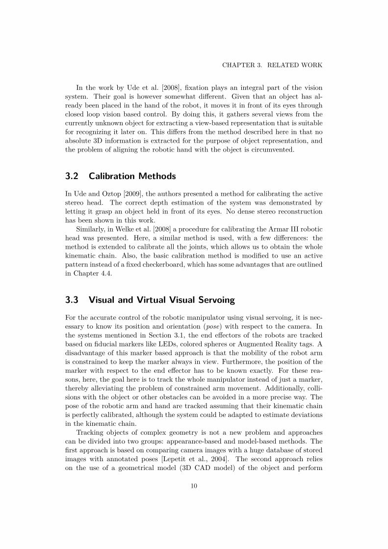
Algorithm 1: Pseudo Code for Defining the Calibration PatternData: Number of points n on each depth plane, number of depth planes mResult: Set of Correspondences

[QA

i , Pi

]with (0 < i ≤ m · n)

begin// Initialising the principal axis of the camera in arm space// VisualServoing(P,S) is a function that brings the LED to// the point P in image space within the plane S in arm spaceS0 = Some plane at a distance d0 from the cameraCA

0 = VisualServoing((0, 0),S0)S1 = Some plane at a distance d1 from the cameraCA

1 = VisualServoing((0, 0),S1)d = (CA

1 − CA0 )/(m− 1)

i = 0foreach l ∈ [0 . . .m− 1] do

S = plane with normal d which contains CA0 + ld

foreach Pk with (0 < k ≤ n) doQA

i = VisualServoing((xk, xy),S)i+ +

endend

end

transformation between the camera coordinate system before and after moving acertain joint from the motor encoders.

In Section 2.2.2, the transformation error that arises from the misalignment ofthe real and ideal coordinate frames of a joint is described. This error is minimisedby finding the true position and orientation of the real coordinate frame as follows:

1. Choose two different positions of the joint, that are far enough apart to besignificant, but with an overlapping viewing area that is still reachable for therobotic arm.

2. For each of these two positions, perform the static calibration process as de-scribed above, so that we obtain the transformation between the arm coordi-nate system and each of the camera coordinate systems.

3. Find the transformation between the camera coordinate systems in the twopreviously chosen joint configurations. This transformation is the result ofrotating the joint around some roughly known axis (it is not precisely knownbecause of mechanical inaccuracies), with a roughly known angle from the mo-tor encoders. From the computed transformation, we can then more exactlydetermine this axis, center and angle of rotation.

This is illustrated in Figure 4.3(b).The results showed that while the magnitude of the angles of rotation differed

significantly from what could be obtained from the kinematic chain, the orientationand position of these axes were quite precise in the specifications. To avoid overlycomplicating the model, only the actual angle α in Equation 2.6 were corrected,

19

CHAPTER 4. THE PROPOSED SYSTEM

camera

image

3D

model

distance

transform

initial

estimation

render

image

edge

extraction

interaction

matrix

visual

servoing

estimated

pose

Figure 4.4. Outline of the proposed model-based tracking system based on VirtualVisual Servoing.

(a) (b)

Figure 4.5. Comparison of robot localization with (right) and without (left) theVirtual Visual Servoing correction.

except for the vergence joints. For these joints, the orientation was also corrected,since here small errors have a large impact in the accuracy of depth estimation.With this, we can minimise the discrepancy between the true and estimated essentialmatrix in Equations 2.3 and 2.5 respectively.

20

4.5. VIRTUAL VISUAL SERVOING

4.5 Virtual Visual ServoingAs mentioned in Sections 1 and 3.3, the system uses Virtual Visual Servoing to refinethe position of the arm and hand in camera space provided by the calibration system.In Figure 4.5, the difference between the estimated arm pose and the corrected oneis visualised. In this section we can find a formalization of the problem and theproposed solution.

The pose of an object is denoted by M(R, t) where t ∈ R(3), R ∈ SO(3). Theset of all poses that the robot’s end–effector can attain is denoted with

TG ⊆ SE(3) = R(3) × SO(3) (4.11)

Pose estimation considers the computation of a rotation matrix (orientation)and a translation vector of the object (position), M(R, t):

M =

r11 r12 r13 TX

r21 r22 r23 TY

r31 r32 r33 TZ

(4.12)

The equations used to describe the projection of a three–dimensional model pointQ into homogeneous coordinates of the image point [x y]T are: X

YZ

= R [Q− t] with [wx, wy, w] = P

XYZ

(4.13)

where P represents the internal camera parameters matrix including focal lengthand aspect ratio of the pixels, w is the scaling factor, R and t represent the rotationmatrix and translation vector, respectively.

This approach to pose estimation and tracking is based on virtual visual servoingwhere a rendered model of the robot parts is aligned with the current image oftheir real counterparts. The outline of the system is presented in Fig. 4.4. Inorder to achieve the alignment, we can either control the position of the part tobring it to the desired pose or move the virtual camera so that the virtual imagecorresponds to the current camera image, denoted as real camera image in the restof this document. Using the latter approach has the problem that the local effectof a small change in orientation of the camera is very similar to a large change inits position, which leads to convergence problems. Therefore, the first approach isused, where synthetic images are rendered by incrementally changing the pose ofthe tracked part. In the first iteration, the position is given based on the forwardkinematics. Then, we extract visual features from the rendered image, and comparethem with the features extracted from the current camera image. The details aboutthe features that are extracted are given in Section 4.5.2.

Based on the extracted features, we define an error vector

s(t) = [d1, d2, . . . , dn]T (4.14)

21

CHAPTER 4. THE PROPOSED SYSTEM

between the desired values for the features and the current ones. Based on s, we canestimate the incremental change in pose in each iteration e(s) following the classicalimage based servoing control loop. This process continues until the difference vectors is smaller than a certain threshold. Each of the steps is explained in more detailin the following sections. Our current implementation and experimental evaluationis performed for the Kuka R850 arm and Schunk Dexterous hand, shown in Fig. 4.6

Figure 4.6. The Kuka R850 arm and Schunk Dexterous Hand in real images andCAD models.

4.5.1 Virtual image generationAs mentioned before, the system uses a realistic 3D model of the robotic parts asits input. This adds the challenge of having to render this model at a high framerate, since our system runs in real time, and several visual servoing iterations mustbe performed for every frame that obtained from the cameras.

To render the image, we use a projection matrix P , which corresponds to theinternal parameters of the real camera, and a modelview matrix M , which con-sists of a rotation matrix and a translation vector. The modelview matrix is thenestimated in the visual servoing loop.

One of the most common CAD formats for objects such as robotic hands areInventor files. There are a number of rendering engines which can deal with suchmodels, but none of them had the performance and flexibility required for this ap-plication, so a new scenegraph engine was developed from scratch, which focuses onrendering offscreen images at a high speed. It was developed directly over OpenGL.It can generate about 1000 frames per second in modern graphics hardware, so it isnot at the moment the bottleneck of the system.

The image is rendered without any texture or lighting, since we are only inter-ested in the external edges of the model. We also save the depth map produced bythe rendering process, which will be useful later for the estimation of the jacobian.

22

4.5. VIRTUAL VISUAL SERVOING

4.5.2 FeaturesThe virtual and the real image of the robot parts ought to be compared in terms ofvisual features. These features should be fast to compute, because this comparisonwill be performed as many times per frame as iterations are needed by the virtualvisual servoing for locating the robot. They should also be robust towards non-textured models.

Edge-based features fulfill these requirements. In particular chamfer distances[Butt and Maragos, 1998] modified to include the alignment of edge orientations[Gavrila, 1998] are well suited for matching shapes in cluttered scenes, and areused in recent systems for object localization [Liu et al., 2010]. This feature issimilar in spirit but more general than other ones used in the field of Virtual VisualServoing. Comport et al. [2006] computes distances between real points and virtuallines/ellipsis instead of virtual points. Klose et al. [2010], Drummond and Cipolla[2002b] search for real edges only in the perpendicular direction of the virtual edge.

The mathematic formulation of our features is the following. After performing aCanny edge detection on real image Iu and virtual image Iv we obtain a set of edgepoints U ,V with their correspondent edge orientations OU ,OV (from the horizontaland vertical Sobel filter). The sets U ,V are split into overlapping subsets Ui,Vi

according to their orientations:

ou (mod π) ∈ [2πi16 ,2π(i+ 1)

16 ]⇒ u ∈ Ui (4.15)

Then for each channel Ui we compute the distance transform [Borgefors, 1986]which will allow us to perform multiple distance computations for the same real setU in linear time with the number of points in each new set V. Based on the distancetransform we obtain our final distance vector s = dcham(v,U) = [d1, d2 · · · dn]Tcomposed by distance estimations for each edge point from our virtual image Iv.

dtransf (p) = minu∈Ui

||p− u||, p ∈ Iu (4.16)

dcham(v,U) = dtransf (v), v ∈ Vi, u ∈ Ui (4.17)s = dcham(v,U), dcham(v,U) < δ (4.18)

The points v ∈ V whose distance is higher than an empirically estimated thresholdδ are considered outliers and dropped from s.

4.5.3 Pose correctionOnce the features have been extracted, we can use a classical visual servoing ap-proach to calculate the correction to the pose, [Hutchinson et al., 1996]. There aretwo different approaches to vision-based control: Position-based control uses imagedata to extract a series of 3D features, and control is performed in the 3D Carte-sian space. In image-based control, the image features are directly used to controlthe robot motion. In this case, since the features are distances between edges in

23

CHAPTER 4. THE PROPOSED SYSTEM

an image for which we have no depth information in the real image, image-basedapproach is used.

The basic idea behind visual servoing is to create an error vector which is thedifference between the desired and measured values for a series of features, and thenmap this error directly to robot motion.

As discussed before, s(t) is a vector of feature values measured in the image,composed by distances between edges in the real and synthetic images Iu, Iv. There-fore s(t) will be the rate of change of these distances with time.

The movement of the manipulator (in this case, the virtual manipulator) can bedescribed by a translational velocity T (t) = [Tx(t), Ty(t), Tz(t)]T and a rotationalvelocity Ω(t) = [ωx(t), ωy(t), ωz(t)]T. Together, they form a velocity screw:

r(t) =[Tx, Ty, Tz, ωx, ωy, ωz

]T(4.19)

We can then define the image jacobian or interaction at a certain instant as Jso that:

s = Jr (4.20)

where

J =[∂s

∂r

]=

∂d1∂Tx

∂d1∂Ty

∂d1∂Tz

∂d1∂ωx

∂d1∂ωy

∂d1∂ωz

∂d2∂Tx

∂d2∂Ty

∂d2∂Tz

∂d2∂ωx

∂d2∂ωy

∂d2∂ωz

......

......

......

∂dn∂Tx

∂dn∂Ty

∂dn∂Tz

∂dn∂ωx

∂dn∂ωy

∂dn∂ωz

(4.21)

which relates the motion of the (virtual) manipulator to the variation in the features.The method used to calculate the jacobian is described in detail below.

However, to be able to correct our pose estimation, we need the opposite: weneed to compute r(t) given s(t).

When J is square and nonsingular, it is invertible, and then r = J−1s. Thisis not generally the case, so we have to compute a least squares solution, which isgiven by

r = J+s (4.22)

where J+ is the pseudoinverse of J , which can be calculated as:

J+ = (JTJ)−1JT. (4.23)

The goal for our task is to have all the edges in our synthetic image match edgesin the real image, so the target value for each of the features is 0. Then, we candefine the error function as

e(s) = 0− s (4.24)

24

4.6. OBJECT GRASPING

which leads us to the simple proportional control law:

r = −KJ+s (4.25)

where K is the gain parameter.

4.5.4 Estimation of the jacobian

To estimate the jacobian, we need to calculate the partial derivatives of the fea-ture values with respect to each of the motion components. When features arethe position of points or lines, it is possible to find an analytical solution for thederivatives.

In our case, the features in s are the distances from the edges of the syntheticimage to the closest edge in the real image. Therefore, we numerically approximatethe derivative by calculating how a small change in the relevant direction affectsthe value of the feature.

As mentioned before, while rendering the model we can also obtain a depthmap. From this depth map, it is possible to obtain the 3D point corresponding toeach of the edges. Each model point v in Iv is a projection of its corresponding 3Dpoint in the model vm. The derivative of the distance described before dcham(v,U), can be calculated for a model point vm with respect to Tx by applying a smalldisplacement and projecting it into the image:

dcham

(P M(vm + εx),U

)−D

(P Mvm,U

)ε

(4.26)

where ε is an arbitrary small number and x is a unitary vector in the x direction.P and M are the projection and modelview matrices, as defined in Section 4.5.1.A similar process is applied to each of the motion components.

4.6 Object grasping

This section explains how the grasping point computed in Section 4.2 and the armpose calculated in Section 4.5 can be combined in order to move the arm so that itcan grasp the object.

After finding the grasping position as a point GC0 in camera space, we move thehead to a position where the whole arm is visible, while keeping the object in thefield of view. Then, the object position (x, y) is found in this new viewpoint usingthe method in Section 4.3. We assume that the z coordinate did not change withthe gaze shift. Therefore, we use the one calculated previously in GC0 . The graspingpoint in camera space for the current viewpoint is then GC1 =

[zx zy z

].

After this, virtual visual servoing allows us to obtain the transformation AAC1

that converts points from camera to arm space, so we can obtain the grasping pointin arm space as GA = AA

C1GC1 . To account for small errors in the measurements,

25

CHAPTER 4. THE PROPOSED SYSTEM

we do not move the arm there directly, but take it first to a position which is a fewcentimeters (15 cm in our experiments) above GA.

Then, the final step is to bring the arm down so that the object lies betweenthe fingers of the hand. We can do this using a simple visual servoing loop. Themovement to be performed is purely vertical. Therefore, we only use a single visualfeature to control that degree of freedom: the vertical distance between the arm andthe grasping point in the image which will be roughly aligned with the vertical axisof the arm. In each iteration, we measure the vertical distance d between the armand the grasping point in the image, and use this as input for a simple proportionalcontrol law:

ry = −kd (4.27)

where ry is the vertical velocity of the arm and k is a gain factor.

26

Chapter 5

Experiments

5.1 Robustness of Virtual Visual ServoingIn order to evaluate the performance of the virtual visual servoing, we need a setupwhere ground truth data was available, so that the error both for the input (edgedetection and initial estimation) and the output (estimated pose) is known. Lackingsuch a setup, experiments were conducted using synthetic images as input. Theseimages were generated using the same 3D model and rendering system used in thevisual servoing loop.

The process used in these experiments was as follows:

• Generate a rendered image of the model at a known pose.

• Add some error in translation and rotation to that pose, and use this as theinitial pose estimation.

• Run the virtual visual servoing loop with the rendered image as input. Insome of the runs, noise was added to the detection of edges, to assess therobustness with respect to certain errors in the edge detection.

• After each iteration, check whether the method has reached a stable point(small correction) and the difference between the detected pose and the knownpose is below a certain threshold. If this is the case, consider it a succesfulrun and store the number of iterations needed.

• If the system does not converge to the known pose after a certain number ofiterations, stop the process and count it as a failed run.

Three sets of experiments were run, each of them focusing on the following kindof input error:

• Translational error. Evaluation of the range of errors in the translational com-ponent of the initial pose estimation that allows the system to converge. Tothat effect, in each run, a translational error was added, of known magnitudeand random direction.

27

CHAPTER 5. EXPERIMENTS

• Rotational error. Evaluation of the range of errors in the rotational componentof the initial pose estimation for which the system converges to the correctresult. For each run, a rotational error was added of known magnitude andrandom direction.

• Error in edge detection. To simulate the effects of wrongly detected edges inthe performance of the system, random errors were added to the edge detectionof the input synthetic image. In each run, the detection of a number of pixelswas shifted a random amount. An example of the result can be seen in Fig. 5.1.

Figure 5.1. Edge detection with artificially introduced error (in 30% of the pixels).

The performance of the VVS system is measured in (i) the number of runs thatfailed and (ii) , for the runs that succeeded, the average number of iterations it tookto do so. These are plotted with respect to the magnitude of the input error. Foreach value of the input error, the system was run 500 times. In each of these runs,the magnitude of the error was kept constant, but the direction (or the particularpixels that were affected in the case of edge detection) was chosen randomly. Also,the whole process was repeated for five different configurations of the joints of thearm.

The rest of the parameters of the process were set as follows:

• The threshold for deciding that the algorithm had converged to the correctpose was 10 mm in translation and 0.5 in rotation.

• The number of iterations after which the run was considered a failure was setto 200.

28

5.2. QUALITATIVE EXPERIMENTS ON THE REAL SYSTEM

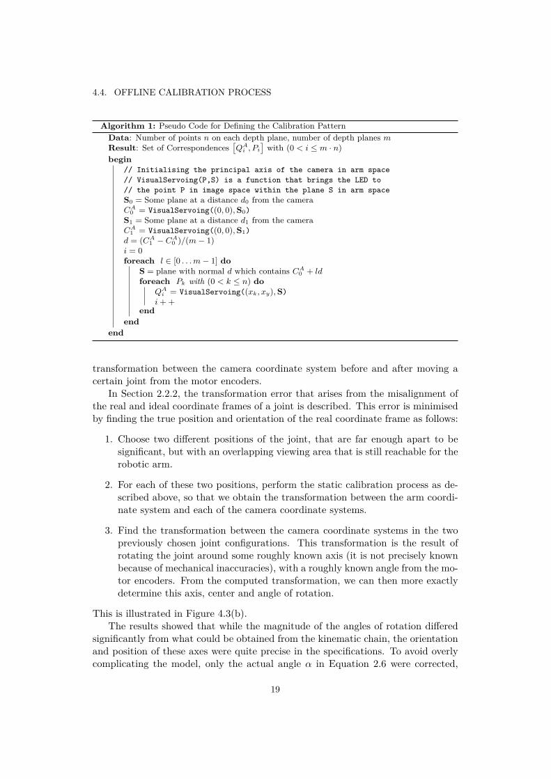
• For the experiments that evaluate robustness with respect to edge detection,a translation error of 100 mm and a rotation error of 10 was used for theinitial pose estimation.

Figure 5.2 shows the result of increasing the translational component of theerror in the estimated initial pose. As we can see, the failure rate is close to 0 fordistances below 100 mm, and then starts increasing linearly. This is probably dueto 100 mm being in the same order of magnitude as the distance between differentedges of the robot which have the same orientation, so the system gets easily lost,trying to follow the wrong edges. We can also observe an increase in the iterationsneeded for reaching the result.

In Figure 5.3 we can observe a similar behaviour for the tolerance to errors in therotational component of the estimated initial pose. Here, the threshold is around10 and the reason is probably the same as before: this is the minimum rotationthat bring edges to the position of other edges.

With respect to the error in edge detection, we can see in Figure 5.4 that whenless than 50% of the pixels are wrongly detected, the system performs almost aswell as with no error, and after that the performance quickly degrades. It is alsosignificant that for the runs that converge successfully, the number of iterations isalmost independent of the errors in edge detection.

0 50 100 150 200 2500

20

40

60

80

mm

numbe

rof

iteratio

ns

0 50 100 150 200 250

0

20

40

60

80

mm

failu

rerate

(%)

Figure 5.2. Effects of translational error

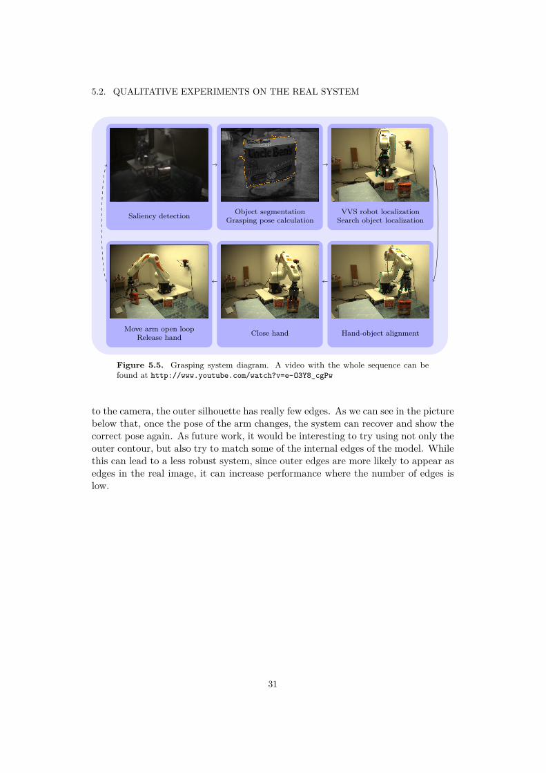
5.2 Qualitative Experiments on the Real SystemFor our experiments with the real robot, two objects are placed randomly on atable-top scenario, as can be seen in the last picture in Figure 5.5. The head wasinitially looking towards the table, where it could see the objects and find them inthe saliency map of the attention system. However, the arm was not fully visible.

The system was then run several times with this setup. In most of these runs,the virtual visual servoing loop did not converge because it could only see a smallpart of the arm. Therefore, the system was modified to use virtual visual servoing

29

CHAPTER 5. EXPERIMENTS

0 10 20 30 40 50

20

40

60

80

100

120

degrees

numbe

rof

iteratio

ns

0 10 20 30 40 50

0

20

40

60

80

100

degrees

failu

rerate

(%)

Figure 5.3. Effects of rotational error

0 20 40 60 80 100

50

100

150

200

pixels affected (%)

numbe

rof

iteratio

ns

0 20 40 60 80 100

0

20

40

60

80

100

pixels affected (%)

failu

rerate

(%)

Figure 5.4. Effects of errors in edge detection

only after the object is found and after shifting the gaze away from it and towardsthe arm. With this change, even if the initial estimation for the pose of the arm wassignificantly different, the pose estimated through visual servoing quickly converged.In Figure 5.5 we can see, outlined in green, the estimated pose for the arm and handover the real image.

The segmentation of the object and detection of the grasping point worked well.When running virtual visual servoing with the full arm in view, the hand could bealigned with the object with high accuracy and grasping was performed successfullyin most of the runs.

However, even if they did not affect the performance of the system, there aresome problems that arise with the use of virtual visual servoing in real images. Forexample, as we can see in the upper-right picture of Figure 5.5, the upper edge ofthe reconstructed outline does not match exactly with the upper edge of the arm.There are two main reasons for this. First, the illumination of the scene can lead tosome edges disappearing, because of the low contrast. This is usually not a problem,because the correct matching of other edges will compensate for this. But in thiscase, there is a second problem: because of the orientation of the arm with respect

30

5.2. QUALITATIVE EXPERIMENTS ON THE REAL SYSTEM

Saliency detection Object segmentationGrasping pose calculation

VVS robot localizationSearch object localization

Hand-object alignmentClose handMove arm open loopRelease hand

Figure 5.5. Grasping system diagram. A video with the whole sequence can befound at http://www.youtube.com/watch?v=e-O3Y8_cgPw

to the camera, the outer silhouette has really few edges. As we can see in the picturebelow that, once the pose of the arm changes, the system can recover and show thecorrect pose again. As future work, it would be interesting to try using not only theouter contour, but also try to match some of the internal edges of the model. Whilethis can lead to a less robust system, since outer edges are more likely to appear asedges in the real image, it can increase performance where the number of edges islow.

31

Chapter 6

Conclusions

Grasping and manipulation of objects is a necessary capability of any robot per-forming realistic tasks in a natural environment. The solutions require a systemsapproach since the objects need to be detected and modelled prior to an agent act-ing upon them. Although many solutions for known objects have been proposed inthe literature, dealing with unknown objects stands as an open problem.

The system described here deals with this problem by integrating the areas ofactive vision and sensor based control where visual servoing methods represent im-portant building blocks. This thesis describes several ways in which these methodscan add robustness and help minimizing the errors inherent to any real system.

First, by using visual servoing to help automate the offline calibration process.The robot can, without human intervention, generate a pattern to collect data thatcan then be used to calibrate the cameras and the transformations between thecameras and the arm.

Then, a virtual visual servoing approach can be used to continuously correctthe spatial relation between the arm and the cameras. Though in its current statethe system works well and is useful in the context of the system, some ideas forfuture work arise from the experiments performed. Using the edges as the onlyfeature in the visual servoing loop works well with objects which have a complexoutline, such as the KUKA arm. However, for other kinds of object, or even someviewpoints of the arm, having a wider range of features might help. These featuresmay include adding textures to the models, or using 3D information obtained viastereo or structured light cameras.

Finally, the last step that brings the arm to the place where the object canactually be grasped also uses visual information to move the arm down to theposition where the hand can be closed to grasp the object. There is also roomfor future improvements here, such as integrating the system with a more complexgrasp planner, which could determine the optimal points where the fingers shouldcontact the object. Then, visual servoing could be used to visually bring the fingersto the correct position.

33

Bibliography

T. Asfour, K. Welke, P. Azad, A. Ude, and R. Dillmann. The Karlsruhe Hu-manoid Head. In IEEE/RAS International Conference on Humanoid Robots(Humanoids), Daejeon, Korea, December 2008.

P. Azad, T. Asfour, and R. Dillmann. Stereo-based 6D Object Localization forGrasping with Humanoid Robot Systems. In IEEE/RSJ Int. Conf. on IntelligentRobots and Systems (IROS), pages 919–924, 2007.

M. Björkman and D. Kragic. Active 3D Segmentation through Fixation of Previ-ously Unseen Objects. In British Machine Vision Conference, September 2010a.To appear.

M. Björkman and D. Kragic. Active 3D Scene Segmentation and Detection of Un-known Objects. In IEEE International Conference on Robotics and Automation,2010b.

J. Bohg and D. Kragic. Learning Grasping Points with Shape Context. Roboticsand Autonomous Systems, 2009. In Press.

G. Borgefors. Distance transformations in digital images. Computer Vision, Graph-ics and Image Processing, 34:344–371, 1986.

M. A. Butt and P. Maragos. Optimum design of chamfer distance transforms. IEEETransactions on Image Processing, 7(10):1477–1484, 1998.

A. I. Comport, D. Kragic, E. Marchand, and F. Chaumette. Robust real-timevisual tracking: Comparison, theoretical analysis and performance evaluation.pages 2841 – 2846, apr. 2005.

A. I. Comport, É. Marchand, M. Pressigout, and F. Chaumette. Real-time marker-less tracking for augmented reality: The virtual visual servoing framework. IEEETrans. Vis. Comput. Graph, 12(4):615–628, 2006.

T. Drummond and R. Cipolla. Real-time visual tracking of complex structures.IEEE Trans. PAMI, 24(7):932–946, 2002a.

T. Drummond and R. Cipolla. Real-time visual tracking of complex structures.IEEE Trans. Pattern Anal. Mach. Intell, 24(7):932–946, 2002b.

35

BIBLIOGRAPHY

J. Felip and A. Morales. Robust sensor-based grasp primitive for a three-fingerrobot hand. In Proceedings of the 2009 IEEE/RSJ international conference onIntelligent robots and systems, IROS’09, pages 1811–1816, 2009.

D. M. Gavrila. Multi-feature hierarchical template matching using distance trans-forms. In ICPR, pages Vol I: 439–444, 1998.

X. Gratal, J. Bohg, M. Björkman, and D. Kragic. Scene representation and objectgrasping using active vision. In IROS’10 Workshop on Defining and SolvingRealistic Perception Problems in Personal Robotics, October 2010.

K. Hsiao, S. Chitta, M. Ciocarlie, and E. G. Jones. Contact-reactive grasping ofobjects with partial shape information. In IEEE/RSJ Int. Conf. on IntelligentRobots and Systems (IROS), pages 1228–1235, Taipei, Taiwan, Oct 2010.

K. Huebner, K. Welke, M. Przybylski, N. Vahrenkamp, T. Asfour, D. Kragic, andR. Dillmann. Grasping Known Objects with Humanoid Robots: A Box-basedApproach. In International Conference on Advanced Robotics, pages 1–6, 2009.

S. Hutchinson, G. Hager, and P. Corke. A tutorial on visual servo control. IEEETransactions on Robotics and Automation, 12(5):651–670, 1996.

A. W. Khan and C. Wuyi. Systematic geometric error modelling for workspacevolumetric calibration of a 5-axis turbine blade grinding machine. Chinese Journalof Aeronautics, pages 604–615, 2010.

S. Klose, J. Wang, M. Achtelik, G. Panin, F. Holzapfel, and A. Knoll. Markerless,vision-assisted flight control of a quadrocopter. In IROS, 2010.

D. Kragic and H. I. Christensen. Cue integration for visual servoing. IEEE Trans-actions on Robotics and Automation, 17(1):18–27, Feb. 2001.

D. Kragic and V. Kyrki. Initialization and system modeling in 3-d pose tracking. InIn IEEE International Conference on Pattern Recognition 2006. ICPR’06, pages643–646, Hong Kong, 2006.

KUKA. KR 5 sixx R850. www.kuka-robotics.com, Last Visited Dec’10.

V. Kyrki and D. Kragic. Integration of model-based and model-free cues for vi-sual object tracking in 3d. In IEEE International Conference on Robotics andAutomation, ICRA’05, pages 1566–1572, 2005.

B. León, S. Ulbrich, R. Diankov, G. Puche, M. Przybylski, A. Morales, T. Asfour,S. Moisio, J. Bohg, J. Kuffner, and R. Dillmann. OpenGRASP: A toolkit forrobot grasping simulation. In SIMPAR ’10: Proceedings of the 2nd InternationalConference on Simulation, Modeling, and Programming for Autonomous Robots,November 2010.

36

BIBLIOGRAPHY

V. Lepetit, J. Pilet, and P. Fua. Point matching as a classification problem for fastand robust object pose estimation. In CVPR, pages II: 244–250, 2004.

M. Liu, O. Tuzel, A. Veeraraghavan, and R. Chellappa. Fast directional chamfermatching. In CVPR, pages 1696–1703. IEEE, 2010.

B. Rasolzadeh, M. Björkman, K. Huebner, and D. Kragic. An Active Vision Sys-tem for Detecting, Fixating and Manipulating Objects in Real World. Int. J. ofRobotics Research, 2009. To appear.

SCHUNK. Sdh. www.schunk.com, Last visited Dec’10.

A. Ude and E. Oztop. Active 3-d vision on a humanoid head. In Int. Conf.onAdvanced Robotics (ICAR), Munich, Germany, 2009.

A. Ude, D. Omrcen, and G. Cheng. Making Object Learning and Recognition anActive Process. Int. J. of Humanoid Robotics, 5(2):267–286, 2008.

N. Vahrenkamp, S. Wieland, P. Azad, D. Gonzalez, T. Asfour, and R. Dillmann.Visual Servoing for Humanoid Grasping and Manipulation Tasks. In IEEE/RASInt. Conf. on Humanoid Robots (Humanoids), pages 406–412, 2008.

K. Welke, M. Przybylski, T. Asfour, and R. Dillmann. Kinematic calibration for sac-cadic eye movements. Technical report, Institute for Anthropomatics, UniversitätKarlsruhe, 2008.

Z. Zhang. A flexible new technique for camera calibration. IEEE Transactions onPattern Analysis and Machine Intelligence, 22:1330–1334, 2000. ISSN 0162-8828.

37

TRITA-CSC-E 2012:013 ISRN-KTH/CSC/E--12/013-SE

ISSN-1653-5715

www.kth.se