Visual Propagation Display

1

Visual Propagation Display

I N S I D E T H I S T U T O R I A L

1 Introduction / Overview

2 Using the Visual Propagation Display

8 Viewing Propagation Results in Google Earth

9 Propagation Display from MFD Search Results

12 Propagation Display using Dynamic Database

Browsing

Introduction This tutorial was designed to introduce Datalinks users to the new Visual Propagation Display tool. This document assumes users are familiar with using the DataLinks system and have an understanding of radio propagation concepts. Users unfamiliar with the DataLinks system may need to refer to Tutorials #1 and #2 before using the tool.

Overview

The Visual Propagation Display feature is an analysis tool for modeling or simulating radio wave signal strength in a specific region. A circular sweep is performed around a transmitter center point extending out to a specified radius. The analysis uses a number of system and user-defined parameters including transmitter specifications, antenna patterns, environmental characteristics and terrain data. The Visual Propagation tool will return a heatmap in multiple output formats that can be used to visualize signal coverage.

Visual Propagation Display

2

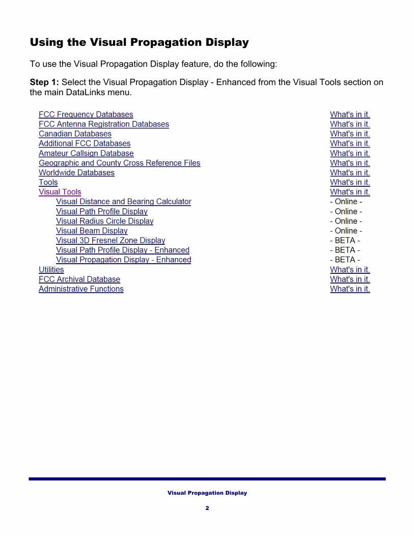
Using the Visual Propagation Display To use the Visual Propagation Display feature, do the following:

Step 1: Select the Visual Propagation Display - Enhanced from the Visual Tools section on the main DataLinks menu.

Visual Propagation Display

3

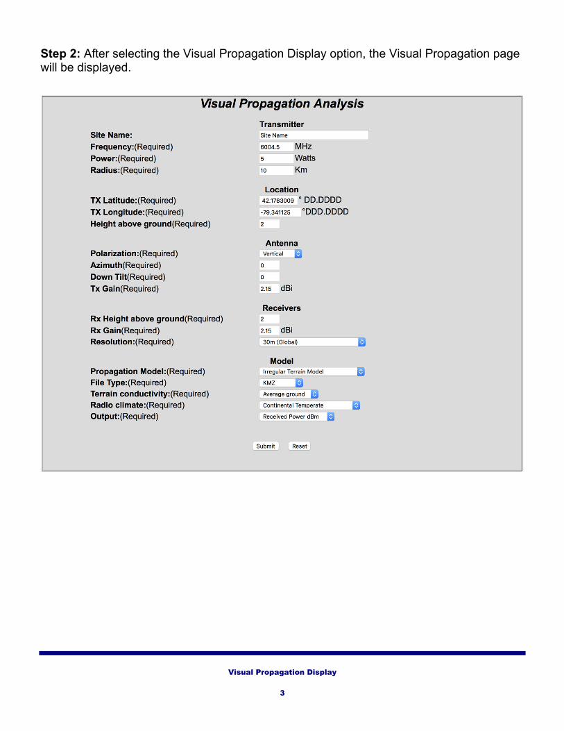
Step 2: After selecting the Visual Propagation Display option, the Visual Propagation page will be displayed.

Visual Propagation Display

4

Step 2 (continued): A path profile analysis requires multiple parameters from several groups. The following parameters are required, unless otherwise noted: Transmitter: Site Name: Site name description used in text output, not required. Frequency: Transmitter frequency in MHz. Power: Transmitter power in watts. Radius: Analysis radius from transmitter in kilometers. Location: TX Latitude: Transmitter latitude in decimal degrees. TX Longitude: Transmitter longitude in decimal degrees. Height above ground: Transmitter height above ground in meters. File Type: Analysis output file type. The following options are available:

KMZ: Google Earth KML file Esri Shape: Esri ArcGIS shape file URL: Link to web-based map HTML: Web-based map embedded in the results page TIFF: Raster image file

Antenna: Polarization: Antenna polarization (orientation), either Vertical or Horizontal. Azimuth: Antenna azimuth in degrees. Down Tilt: Antenna down tilt in degrees. TX Gain: Transmitter gain in dBi. Receivers: RX Height above ground: Receiver height above ground in meters. RX Gain: Receiver gain in dBi. Resolution: Digital terrain/surface model resolution. The following options are available:

30m (Global): SRTM2 (Shuttle Radar Topography Mission, ver. 2) from 2000, 30m resolution with global coverage.

90m (Global): SRTM2 (Shuttle Radar Topography Mission, ver. 2) from 2000, 90m resolution with global coverage up to 60 degrees North.

1m Lidar (subject to availability): High resolution, plane and drone-mapped 1m resolution for select areas.

2m Lidar (subject to availability): High resolution, plane and drone-mapped 2m resolution for select areas.

16m Lidar (subject to availability): High resolution, plane and drone-mapped 16m resolution for select areas.

Visual Propagation Display

5

Lidar (continued) Lidar coverage areas include the following locations: North America: United States: New York, Los Angeles, San Francisco, San Diego, Washington DC, Philadelphia, Baltimore Lidar Coverage (continued) Europe: United Kingdom Australia: Sydney, Brisbane, Westcoast Australia. Christchurch New Zealand Asia: Nepal Model: Propagation Model: Radio propagation model. Users can select from the following models:

Irregular Terrain Model - (Longley Rice Model) General purpose model used by FCC. (20 MHz to 20 GHz).

SUI Microwave (1.9-11GHz) - Stanford University Interim for WiMAX communications. (1.9 to 11 GHz).

Line of Sight - Simple model for viewing obstructions in any frequency range. Okumura-Hata (0.15-1.5GHz) - Model for cellular communications in urban areas.

(150 to 1500 MHz). ECC33 (ITU P.529) (0.15-3.5GHz) - Model for cellular and microwave

communications. (700 MHz to 3.5 GHz) COST231-Hata (0.15-2GHz) - European COST231 frequency extension to Hata

model for urban areas. (150 MHz - 2.0 GHz) Free Space Path Loss (ITU P.525) - Free space model that assumes no obstacles

exist between the transmitter and the receiver(s). ITWOM 3.0 - Irregular Terrain Model with obstructions 3.0 model. Ericsson 9999 (0.15-1.9GHz) - Model for cellular communications. (150 MHz to 1900

MHz) Plane Earth Loss - Modified free space model that incorporates the reflected power

from the ground. Egli VHF/UHF - General purpose VHF/UHF model that is more conservative than the

Free Space Loss Model, but more optimistic than the Hata/COST models.

Visual Propagation Display

6

Model (continued) Terrain Conductivity: Terrain conductivity (or ground conductivity) is the electrical conductivity of the terrain. Users should select one of following options that best describes the area of analysis. The following options are available:

Water Wet ground Farmland Forest Average ground Mountain / Sand Marsh City Poor ground

Radio Climate: Users should select one of following options that best describes the climate of the area of analysis. The following options are available:

Continental Temperate Maritime Temperate (sea) Maritime Temperate (land) – Over land (UK and west coasts of US and EU) Equatorial (Congo) Continental Subtropical (Sudan) Maritime Subtropical (W. Africa) – West coast of Africa Desert (Sahara)

Output: Output measurement units. Users can select from the following options:

Path Loss – dB Received Power – dBm Field Strength – dBuV/m

After entering the desired parameters, click the Submit button to run the propagation study. Click the Reset button to reset the parameters to the original default settings.

Visual Propagation Display

7

Step 3: After the Propagation analysis is complete, a results page will be displayed.

The results page will contain a summary of the parameters used for the analysis and a link used to save the output file. The link will vary depending on File Type selected. PC users can right-click on the link to save the file and Mac OS users can use a CTRL click to save the file. Google Earth .KMZ: After saving the file to a local drive, double-click on the file to launch Google Earth with the .kmz file data. Esri ArcGIS shape file: The shape file results are returned in a .zip file. After saving the file to a local drive, double-click on the .zip file and then launch ArcGIS to open the decompressed .zip file containing SHP data. .TIFF Raster image: After saving the .TIFF file to a local drive, use any graphics program capable to reading a .tiff file to view or edit. URL: The results page returns a link to web page containing a map with the propagation overlay. HTML: Similar to the URL output with the map embedded in the output page.

Visual Propagation Display

8

Viewing Propagation Results in Google Earth After launching Google Earth with the propagation results .KMZ file, Google Earth will automatically zoom to the propagation analysis area.

The results objects can be found in the Places window under Temporary Places. There will be a main entry which can be expanded by clicking on the arrow on the left side. There are several sub entries for the main propagation heatmap overlay including the color key, transmitter icon and details that can be toggled on or off for display by unchecking the corresponding check box next to each entry.

Using the various Google Earth features, users can rotate, zoom and pan the map to view the simulated coverage shown in the propagation heatmap. Note: To ensure the path profile displays properly, the Terrain checkbox in the Layers window should be checked (enabled) at all times.

Visual Propagation Display

9

Propagation Display from MFD Search Results

Datalinks users can perform a propagation analysis from Master Frequency Database (MFD) searches by selecting the Brief w/ Links output option. To perform a propagation study from an existing MFD search, do the following:

Step 1: Select the FCC Master Frequency Database (MFD) from the FCC Frequency Databases menu.

Step 2: Select a search from the list of available searches. For this example, a Callsign search is used.

Visual Propagation Display

10

Step 3: Enter the desired parameters for the search. Select the Brief w/ Links for the Output Format. Click the Submit button to run the search.

Step 4: When the search is complete, the results page will display the output data. Many of the fields include links that can be used to display additional data or perform another search. The last field, “PROP”, includes a link can be used to perform a Visual Propagation analysis for that transmitter.

Visual Propagation Display

11

Step 5: After clicking the link, a new Visual Propagation entry screen will be displayed, but will be preformatted using the data from the transmitter selected.

Step 6: After the analysis is complete, the results summary and file download link will be displayed. Users can save the output file and open with the appropriate application for further study.

Visual Propagation Display

12

Propagation Display using Dynamic Database Browsing

Datalinks users can also perform a propagation analysis using the Dynamic Database Browsing feature included in .KML output files from Master Frequency Database (MFD) searches. To perform a propagation study using Dynamic Database Browsing, do the following:

Step 1: Select a database from the FCC Frequency Databases menu. Step 2: Select a search from the list of available searches.

Step 3: Enter the parameters for the search. Select the Google Earth - KML option for the Output Format. Click the Submit button to run the search.

Step 4: When the search is complete, save the linked .KML file and double-click on the file to launch Google Earth using the search results. Step 5: After Google Earth launches, click on any transmitter point to display the details window for that location.

Visual Propagation Display

13

Step 6: The details window includes a “Click to see a propagation analysis” link. Clicking the link will open a Visual Propagation entry screen within Google Earth. The entry screen parameter will be preformatted using data from the selected transmitter. After setting the desired parameters, click the Submit button to begin the analysis using the default web browser.

Step 7: After the analysis is complete, the results summary and file download link will be displayed. Users can save the output file and open with the appropriate application for further study.

Visual Propagation Display

14

Company Information PerCon Corporation 4906 Maple Springs / Ellery Rd. Bemus Point NY 14712 (716)386-6015 (716)386-6013 FAX http://www.perconcorp.com email: sales@perconcorp.com

Related Documents:

Introduction to DataLinks

Google Earth (KML) Output Files

Dynamic Database Browsing

Propagation Analysis http://www.perconcorp.com/support.html