University of Nebraska - LincolnDigitalCommons@University of Nebraska - Lincoln

U.S. Environmental Protection Agency Papers United States Environmental Protection Agency

1-1-2004

Visual Plumes mixing zone modeling softwareWalter E. FrickU.S. EPA, frick.walter@epa.gov

Follow this and additional works at: http://digitalcommons.unl.edu/usepapapers

This Article is brought to you for free and open access by the United States Environmental Protection Agency at DigitalCommons@University ofNebraska - Lincoln. It has been accepted for inclusion in U.S. Environmental Protection Agency Papers by an authorized administrator ofDigitalCommons@University of Nebraska - Lincoln.

Frick, Walter E., "Visual Plumes mixing zone modeling software" (2004). U.S. Environmental Protection Agency Papers. Paper 166.http://digitalcommons.unl.edu/usepapapers/166

Environmental Modelling & Software 19 (2004) 645–654www.elsevier.com/locate/envsoft

Visual Plumes mixing zone modeling software5

Walter E. Frick �

Ecosystems Research Division, NERL, ORD, U.S. EPA, 960 College Station Road, Athens, GA 30605, USA

Received 11 March 2002; received in revised form 20 May 2003; accepted 8 August 2003

Abstract

The US Environmental Protection Agency has a history of developing plume models and providing technical assistance. TheVisual Plumes model (VP) is a recent addition to the public-domain models available on the EPA Center for Exposure Assess-ment Modeling (CEAM) web page. The Windows-based VP adapts, modifies, and enhances the earlier DOS-based PLUMESwith a new interface, models, and capabilities. VP is a public platform for mixing zone models designed to encourage the con-tinued improvement of plume theory and models by facilitating verification and inter-model comparison. Some examples are pre-sented to illustrate VP’s new capabilities. One demonstrates its ability, for reasonably one-dimensional estuaries, to estimatebackground concentrations due to tidal re-circulation of previously contaminated receiving water. This capability depends on theoptional linkage to time-series input files that enables VP to simulate mixing zone and far-field parameters for long periods. Alsodescribed are the new bacterial decay models used to estimate depth changes in first-order decay rates based on environmentalstressors, including solar insolation, salinity, and temperature. The nascent density phenomenon is briefly described as it is poten-tially important to Outer Continental Shelf (OCS) oil exploration discharges.# 2003 Elsevier Ltd. All rights reserved.

Keywords: Plumes; Outfalls; Density stratification; Bacteria; Dilution; Mathematical models

1. Introduction

Public-domain environmental software provides a

way for the regulated and the regulatory communities

to develop projects in an environmentally sound way

and to assess both proposed projects and changes to

existing facilities. For designing and assessing waste-

water discharges to marine and fresh surface waters,

Visual Plumes exemplifies this model. Introduced in

September 2001, Visual Plumes, software and guidance,

is available through the EPA Center for Exposure

Assessment Modeling web page (CEAM, 2001). After

installing the program, users are encouraged to obtain

the latest version of the executable from the author viaemail: frick.walter@epa.gov.Visual Plumes (VP) uses a familiar Windows-based

graphical user interface for model execution and out-put visualization. The user provides the required infor-mation describing the discharge through three inputwindows (represented by simulated file tabs, see Figs. 1–3). Both standard, primarily SI, and many nonstandardunits may be used. Once familiar with the program,single runs are easy to set up, however, for in-depthanalyses, Visual Plumes was designed to handle mul-tiple runs. This is achieved by allowing appropriatetime-series files to be linked to the project at hand. Theuser may review and manipulate model output, bothtext based and graphical, using the graphical interface.This paper describes some of the major Visual

Plumes features, develops a time-series example todemonstrate its advanced capabilities, and offers someopinions on outstanding topics of interest, includingproblems encountered in the oil industry: re-circu-lation, nascent density, and paradigmatic scientificissues.

5 This document has been reviewed in accordance with the US

Environmental Protection Agency’s peer and administrative review

policies and approved for publication. Mention of trade names or

commercial products does not constitute endorsement or recommen-

dation for use.� Tel.: +1-706-355-8319; fax: +1-706-355-8302.

E-mail address: frick.walter@epa.gov (W.E. Frick).

1364-8152/$ - see front matter # 2003 Elsevier Ltd. All rights reserved.

doi:10.1016/j.envsoft.2003.08.018

Fig. 1. Visual Plumes’ Diffuser tab for the oil well project.

Fig. 2. The Ambient tab for the Dominguez Channel project.

646 W.E. Frick / Environmental Modelling & Software 19 (2004) 645–654

2. Visual Plumes

Visual Plumes (Frick et al., 2002; CEAM, 2001) is a

Windows-based program for predicting the dispersive

and other physical processes affecting surface water

effluents: plumes and jets. Like its DOS-based prede-

cessor, PLUMES (Baumgartner et al., 1994), Visual

Plumes (VP) supports multiple initial dilution and far-

field models that simulate single and merging sub-

merged plumes in arbitrarily stratified ambient flow.

The initial dilution models primarily focus on sub-

merged discharges include DKHW, NRFIELD, and

UM3. In addition, there is the PDS surface discharge

model. Finally, the Brooks algorithm is used to predict

far-field centerline dilution and waste field width. Thus

Visual Plumes has a two-fold character, a common

graphical interface supporting multiple models that

may be selected individually by the user.The names of the models provide a mix of acronyms,

and, historical and descriptive terms. The DKHW

model name incorporates author initials and the letter

‘‘W’’ to signify Windows. UM3 is a three-dimensional

model based on the earlier UM (Baumgartner et al.,

1994) and UMERGE models (Muellenhoff et al.,

1985). The RSB model (Baumgartner et al., 1994) is

renamed NRFIELD, the new name anticipating future

changes.

Visual Plumes provides a convenient way to compare

model performance. The support of multiple models

represents a commitment to a public modeling plat-

form that will foster scientific competition by encour-

aging modelers to continue to improve their

applications. The ability to run different models con-

secutively and display the results in graphical form is

designed to facilitate model comparison and develop-

ment. (For 3-D plume depictions, see Lee and Wang,

2002).Visual Plumes predicts several standard quantities,

including dilution, rise, diameter, and other plume vari-

ables. But it also has important new capabilities,

including multi-stressor bacterial decay models, gra-

phics, time-series input, rudimentary sensitivity analy-

sis, user-specified units, and a tidal background

pollutant build-up capability.VP is backward compatible to support users of DOS

PLUMES who wish to revise existing projects or take

advantage of previous features, like computing length-

scale, similarity parameters, and related input variables

not explicitly supported by VP. DOS PLUMES is one

of the ‘‘models’’ that can be run by VP. VP prepares

the necessary PLUMES input file and displays the out-

put. It also reads PLUMES input files (files with the

VAR extension).

Fig. 3. The Special Settings tab for the Dominguez Channel project.

W.E. Frick / Environmental Modelling & Software 19 (2004) 645–654 647

While it is easy to run single scenarios, VP isdesigned for multiple cases. In this regard, perhaps noother capability sets VP apart more from earlier pro-grams than its ability to link in ASCII time-seriesfiles. This capability provides a way to simulate outfallperformance over long periods of time and, thereby,over many environmental scenarios. This is the heart ofthe pollutant-buildup capability, the ability in one-dimensional tidal rivers or estuaries to estimate back-ground pollution due to the source itself. Predictionsare displayed graphically to show overall time-seriesperformance.Technical support experience shows that VP is not

particularly intuitive to use. It is easy to complete theinterface and run the models but its very flexibility canbe confusing. Some of this is due to the fact that somecomponents appear on the interface even when theirfunctions are not utilized. For example, the optionaltime-series linkage windows are always displayed evenwhen no files are linked. Many specialized input vari-ables are found on the special settings tab. Variablelists for specifying output files show abbreviated namesthat are not very descriptive. It is not always clearwhich components possess special capabilities accessedthrough left or right clicking. The context-sensitivehelp system is incomplete, and so on. Hopefully futurechanges will remove or mitigate some of these annoy-ing characteristics. For technical assistance call theauthor (706/355-8319) or email (frick.walter@epa.gov).

3. Interface appearance

The VP Windows-based graphical interface is orga-nized around stacked tabs. The diffuser tab, displayedwhen VP starts, is devoted to overall program controland diffuser and flow input. The completed diffuser tabfor the oil well project further developed below isshown in Fig. 1. Note that VP allows non-SI units tobe specified; for example, the flow of 10 000 barrels perday shown in the diffuser table, the large block in themiddle of the tab, corresponds to 0.0184 m3 s�1. Non-standard units may be selected by clicking on the col-umn unit label to reveal a list of available units. Manycustomized settings are maintained in a project ‘‘list’’file that bears the project name followed by the ‘‘lst’’extension. Blank cells in the table either indicate thatthe column is not required (labeled n/r) or, if multiplecases are indicated on successive lines in the table, thevalue is the same as the one in the previous row. Thusthe single additional value on the second line, 38.489C,is all that is required to represent another flow scen-ario. Note that the flow variables (brown background)starting with Port depth may be time-series variables,however, in this project none of the five variables are

linked in as can be established from the empty Time-series file array at the bottom.The Model Configuration panel settings control the

way VP models, particularly the ‘‘native’’ UM3 model,run and simulation text and graphics are displayed.For example, the ambient file list identifies two associa-ted ambient files. The ‘‘Sequential, all ambient list’’op-tion on the Case selection panel, instructs VP to do allnine cases when a model is selected to run.The ambient conditions (for Dominguez Channel

project using time-series input) are specified on theambient tab shown in Fig. 2. In this relatively simpleapplication, all variables have constant values exceptfor current speed and current direction that are readfrom the linked-in ASCII data files: Dominguez Ch.spdand Dominguez Ch.dir. Evidence of the linkage isreflected by filled cells in the Time-series Files array atthe bottom of the tab. The ambient table units for thespeed and direction columns are changed to meters andnow specify the measurement depths of the input data.Specifying time-series input data at the same depthsgiven in the ambient table allows the direct loading ofVP’s internal ambient array, bypassing the databasefunctions that are normally necessary to interpret theambient input table, thereby speeding the simulation ofmany runs.The Special Settings tab (for Dominguez Channel

project) is given in Fig. 3. Most noteworthy here is thedisplay of the UM3-tidal-pollutant-buildup-parameterscells. Most of the cells on the UM3 tidal pollutantbuildup panel are only visible when the Tidal pollutantbuildup option is checked on the Model Configurationpanel on the diffuser tab.

4. Time-series input

One of VP’s advanced features is the time-series datainput capability. While worst case scenarios have beena mainstay of mixing zone analysis, increasingly usersare interested in the continuous performance of out-falls, for example, they may be interested in statisticalmeasures. Also, worst case analysis can be misleading,for example, at fixed distances from the source, like amixing zone boundary, the highest concentrations arefrequently associated with moderate currents (Baum-gartner et al., 1994), not with zero currents as com-monly believed. The time-series data input capabilityfacilitates such analysis by making multiple VP runsrelatively easy to set up and execute.In the normal VP input mode, the user provides

input for a single case or several cases by manuallyadding the required data to the diffuser and ambienttabs, also setting up and specifying other settings andvariables, particularly on the Special Settings tab. Mul-tiple ambient scenarios may be created by using the

648 W.E. Frick / Environmental Modelling & Software 19 (2004) 645–654

File command, ‘‘Save ambient file as’’ option; this cre-ates a new file that can be modified using the old oneas a template.When linking to time-series data files the diffuser

table may only specify a single case and there may beonly a single ambient file associated with the project.The time-varying input will be contained in one or sev-eral files linked to the project through the optionalTime-series files panels on the diffuser and ambienttabs.Once data are formatted in the prescribed fashion,

VP can read the time-series files in place of the inputtable and provide the corresponding prediction andoutput. In this way it can analyze many cases in a sys-tematic fashion. The additional time and effort (whichdepends on the amount of data manipulation requiredto get the time-series into VP compatible format) maythen be recovered by avoiding the numerous ambientinput files that would otherwise be required.

5. Tidal pollutant buildup theory

Experience shows that one of the greatest pitfalls forusers of initial dilution models is to be unaware of thedifference between dilution and effective dilution. Thisis a problem because models have historically reportedvolume dilution that estimates the relative mixture ofambient and effluent water, not emphasizing the ratioof effluent to plume concentration.Visual Plumes considers two dilution measures, vol-

ume dilution, Sa, defined as

Sa ¼me þ ma

með1Þ

where ve is the initial volume of the plume element (orcontrol volume) and va is the volume of ambient waterincorporated into the plume element in the dilutionprocess, and, effective dilution, Seff defined as

Seff ¼cecp

¼ 1

1

Saþ ca

ce

ð2Þ

where ce is the effluent pollutant concentration, cp isthe plume element concentration at the point of inter-est, and ca is the ambient concentration (Baumgartneret al., 1994). If ca is zero then Sa¼Seff , otherwise theeffective dilution is typically less than the volumedilution. Effective dilution underscores the fact that acomplete mass balance of the dilution process includesthe pollutant mass originating in the dilution water. Asan example, effluent and ambient concentrations of 100ppm and 10 ppm, respectively, limits effective dilutionto 10, even if volume dilution far exceeds that value.The ambient pollution level puts a lower limit on theconcentration that can be achieved by mixing.

If the source contributes to the buildup of ambientconcentration in the surface water the effective dilutioncan degrade over time. It may be the failure in theearly 1990s to adopt the effective dilution as the correctmeasure to protect surface waters that may have con-tributed to the fact that many NPDES permits subse-quently failed to protect water quality. The TotalMaximum Daily Loading (TMDL) process nowaddresses this problem separately.One way to enable VP to predict effective dilution is

to supply ambient concentrations. However, this canbe not only tedious, if there are many cases, but ambi-ent measurements are often unavailable. For relativelysmall, tidal estuaries that are reasonably one-dimen-sional, VP has a simple way for estimating the buildupof background pollution due to the presence of thesource itself. The approach is fairly simple, ignoringthe influence of most of the channel details, like mor-phology and dispersion, on the distribution of pollu-tants. The approach is used in conjunction with thetime-series capability. Necessary data includes thecross-sectional area of the channel at the point of dis-charge and the water velocity in the channel as a func-tion of time. The manual should be consulted foradditional details.The approach is mass conservative, however, an

important underlying assumption is that no redistri-bution of carrier water from the source is necessary. Inother words, all volume contributed by the source ismaintained in the fetch element to which it was dis-charged whenever the element passes over the point ofdischarge. This continues until the element ceases topass over the discharge due to the presence of fresh-water flow or until it reaches open water. Thus,unnatural water elevations can be implied by thisapproach that would not occur if the discharged waterwere routed by a hydrodynamic model. As a result,comparison between measured and observed con-centrations at any given time may be adversely affected.However, considered statistically, over a long period oftime the approach is expected to give realistic results.For example, while dispersion is not included, the factthat dispersion has symmetry, transporting pollutantboth upstream and downstream, suggests that waterflowing into the source region from upstream will reachconcentrations comparable to those obtained by ignor-ing dispersion and allowing polluted water to flow upand down stream with the tides. While a predicted highconcentration may not be observed at the stated time,such a measurement is likely if flow conditions con-tinue to follow the same pattern. The predictions willbe representative of conditions in general.This buildup approach is most representative when

the source is isolated from other sources, so that‘‘natural’’ background is easily defined, and when thesource is sufficiently far upstream so that a fetch

W.E. Frick / Environmental Modelling & Software 19 (2004) 645–654 649

element does not reach the mouth of the channel dur-ing a single tidal cycle. If the natural background isknown as a function of time it would be entered as atime-series file and the tidal buildup algorithm wouldbe turned off.

6. A tidal channel discharge

The Dominguez Channel example is based on anactual project. The city of Los Angeles, parts of whichare situated on a large, low-lying coastal plain, plans tobuild a rail system between the harbor and downtown,a distance of about 30 km. Much of the right-of-waywould be excavated below the water table, necessitatingthe removal of large volumes of groundwater duringconstruction. The original plan was to discharge it toDominguez Channel, requiring the issuance of aNational Pollution Discharge Elimination System(NPDES) permit. As an old industrial center, thegroundwater is unusually high in heavy metals, raisingthe possibility that water quality criteria in DominguezChannel could be exceeded.The initial mixing zone model runs indicated that

water quality criteria would be met, however, theseanalyses did not consider the potential buildup ofbackground pollution. To estimate it with VP it isnecessary to establish the water velocity at the dis-charge point. Available information on the project

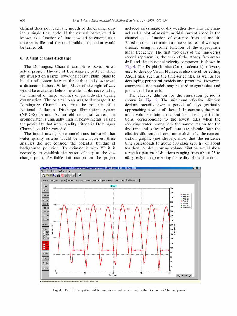
included an estimate of dry weather flow into the chan-nel and a plot of maximum tidal current speed in thechannel as a function of distance from its mouth.Based on this information a time-series record was syn-thesized using a cosine function of the appropriatelunar frequency. The first two days of the time-seriesrecord representing the sum of the steady freshwaterdrift and the sinusoidal velocity component is shown inFig. 4. The Delphi (Inprise Corp. trademark) software,used to develop Visual Plumes, is also useful for editingASCII files, such as the time-series files, as well as fordeveloping peripheral models and programs. However,commercial tide models may be used to synthesize, andpredict, tidal currents.The effective dilution for the simulation period is

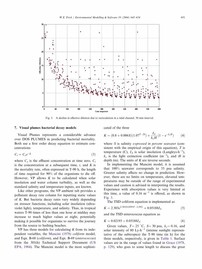
shown in Fig. 5. The minimum effective dilutiondeclines steadily over a period of days graduallyapproaching a value of about 3. In contrast, the mini-mum volume dilution is about 25. The highest dilu-tions, corresponding to the lowest tides when thereceiving water moves into the source region for thefirst time and is free of pollutant, are offscale. Both theeffective dilution and, even more obviously, the concen-tration graphic (not shown), show that the residencetime corresponds to about 500 cases (250 h), or aboutten days. A plot showing volume dilution would showa regular pattern of dilutions ranging from about 25 to60, grossly misrepresenting the reality of the situation.

Fig. 4. Part of the synthesized time-series current record used in the Dominguez Channel project.

650 W.E. Frick / Environmental Modelling & Software 19 (2004) 645–654

7. Visual plumes bacterial decay models

Visual Plumes represents a considerable advance

over DOS PLUMES in predicting bacterial mortality.

Both use a first order decay equation to estimate con-

centrations

Ct ¼ Coe� t

K ð3Þ

where Co is the effluent concentration at time zero, Ct

is the concentration at a subsequent time, t, and K is

the mortality rate, often expressed in T-90 h, the length

of time required for 90% of the organisms to die off.

However, VP allows K to be calculated when solar

insolation and water column turbidity, as well as the

standard salinity and temperature inputs, are known.Like other programs, the VP ambient tab provides a

pollutant decay rate column for inputting static values

of K. But bacteria decay rates vary widely depending

on stressor functions, including solar insolation (ultra-

violet light), temperature, and salinity. Thus, in tropical

waters T-90 times of less than one hour at midday may

increase to much higher values at night, potentially

making it possible for organisms to survive the journey

from the source to bathing beaches.VP has three models for calculating K from its inde-

pendent variables, the Mancini (1978) coliform model,

and Eqn. B-68 (coliform), and Eqn. B-69 (enterococcus)

from the 301(h) Technical Support Document (US

EPA, 1984). The Mancini model is the most sophisti-

cated of the three

K ¼ ð0:8þ 0:006SÞð1:07T�20Þ þ IAkeH

ð1� e�keHÞ ð4Þ

where S is salinity expressed in percent seawater (con-sistent with the empirical origin of this equation), T istemperature (C), IA is solar insolation (Langleys-h�1),ke is the light extinction coefficient (m�1), and H isdepth (m). The units of K are inverse seconds.In implementing the Mancini model, it is assumed

that 100% seawater corresponds to 33 psu salinity.Greater salinity affects no change in prediction. How-ever, there are no limits on temperature, elevated tem-peratures may be outside of the range of experimentalvalues and caution is advised in interpreting the results.Experience with absorption values is very limited atthis time, a value of 0.16 m�1 is offered, as shown inFig. 3.The TSD coliform equation is implemented as

K ¼ 2:303e2:303ð0:0295T�2:292Þ þ 0:05188IA ð5Þ

and the TSD enterococcus equation as

K ¼ 0:02193þ 0:05188IA ð6ÞGiven values, T¼ 25

vC, S¼ 30 psu, ke¼ 0:16, and

solar intensity of 80 Ly-h�1 (intense sunlight represen-tative of the subtropics) the T-90 time (in h) for thethree models, respectively, is given in Table 1. Surfacevalues are in the range of values found in Grace (1978,p. 129), who goes to some length to discuss the great

Fig. 5. A decline in effective dilution due to recirculation in a tidal channel, 30 min interval.

W.E. Frick / Environmental Modelling & Software 19 (2004) 645–654 651

uncertainty associated with bacterial decay estimates.

The agreement between the Mancini model and Eqns.

B-68 and B-69 is quite satisfying, and, it can be said

that, at a minimum, VP offers an objective approach to

estimated decay rates. The influence of the primary

stressor, ultra-violet radiation, is apparent.When executing, VP uses surface values of solar

intensity, in conjunction with the light absorption coef-

ficient on the Special Settings tab, to estimate decay

rates at depth. However, inputting surface solar inten-

sity values at all levels on the ambient tab allows com-

putation of the corresponding decay rate through the

units conversion facility. The capability was exploitedin creating Table 1.

8. Thermal discharges and oil well brines

The little-known nascent density effect (Baumgartneret al., 1994) illustrates a potential problem with usinglinear similarity theory to categorize flow. Thisphenomenon attributed to the non-linear equation ofstate for water is appropriately addressed by VP. Ther-mal discharges and oil well drilling brines often exhibitthe phenomenon, due to the range of salinities andtemperatures encountered. This unusual behaviordepends on the initial properties of the effluent, as wellas on the properties of the ambient receiving water. Inextreme cases, plumes that are initially buoyant becomenegatively buoyant and can sink to the bottom insteadof trapping or rising to the surface.The simplest analogy to the nascent density effect in

plumes is pond overturning in winter. It is well knownthat the equation of state for water is non-linear.Unlike most substances that contract continuouslyupon cooling, fresh water expands before freezing

Table 1

Decay times for three models. (T-90 time in h; time in which 90% of

organisms are predicted to die off.)

Depth Mancini model

(coliform)

Eqn. B-68

(coliform)

Eqn. B-69

(enterococcus)

Surface 0.67 0.55 0.55

10 m 1.32 1.08 1.10

20 m 2.13 1.76 1.81

50 m 4.65 3.95 4.26

100 m 8.02 7.11 8.18

Fig. 6. Density diagram for water as a function of salinity and temperature. Three mixing lines are shown for a warm brine, a sewage effluent,

and a thermal discharge. All except the sewage effluent exhibit nascent density effects.

652 W.E. Frick / Environmental Modelling & Software 19 (2004) 645–654

below about 4vC. A pond warming slowly in late win-

ter may overturn because, as the surface water warms

above 0vC, it becomes denser than the bottom water

with the result that the pond will suddenly ‘‘overturn’’,

with denser, but warmer, surface water replacing the

colder, but less dense, bottom water.A similar principle can have profound effects on

thermal plumes (Frick and Winiarski, 1978). Consider

a fresh water thermal discharge at 60vC to a uniformly

cooled lake at 0vC. The temperature in the plume will

cool continuously to zero as it mixes in lake water, see

Fig. 6. The density will increase correspondingly, and

the plume will begin to rise, until the average plume

temperature approaches approximately 8vC. However,

below that temperature the plume’s density will be

greater than the ambient density at 0vC and the plume

will first decelerate its upward motion, reverse, and

finally sink to the bottom.For a long time it was believed that the nascent den-

sity effect was potentially important only in cold, fresh

receiving water. Many discharges, like the sewage efflu-

ent in Fig. 6, behave in the traditional way. However,

some DOS PLUMES users found other conditions in

which the nascent density effect is important. Fig. 6

shows the mixing line for a brine, perhaps derived from

a water desalination process, discharged to ocean

water. It is discharged at about 42vC and 43 psu. It is

initially and briefly buoyant, but, at below about 28vC

(dilution about 2:1) it becomes and remains denser

than the ambient density. This characteristic of initial

buoyance followed by high relative density (a process

related to double diffusion) led to this process being

called the nascent density effect (Baumgartner et al.,

1994).Fig. 7 shows plume dilutions at maximum rise of

eight simulated effluents all possessing the same buoy-

ancy on discharge. The temperature ranges from 0 to

70vC in 10

vC increments but the effluent density is 12

sigma-T units, or 1012 kg/m3, in all cases, with sali-

nities adjusted accordingly (ranging from 15 to 47.7

psu). There are three ambient scenarios (files) of vary-

ing density stratification for a total of 24 cases. The

discharge-level ambient density is approximately 1015.4

kg/m3. All eight effluents have the same densimetric

Froude number, and, according to similarity theory,

should form three identical plumes, one for each ambi-

ent scenario. However, as is clear from Fig. 7,

maximum-rise dilutions vary widely.

Fig. 7. Variations in predicted maximum rise dilutions for eight effluents described by three densimetric Froude numbers. (Each set of eight

simulations corresponds to one of three ambient stratification scenarios.) (Simulations: red squares = DKHW, green = UM3.)

W.E. Frick / Environmental Modelling & Software 19 (2004) 645–654 653

9. Conclusion

Visual Plumes is a Windows-based public domainsoftware available through the Center for ExposureAssessment Modeling web page (CEAM, 2001). It isuseful for predicting plume dilution and physicalproperties, both in the mixing zone and in the far field.Simple scenarios are relatively easy to set up and run,however, its real strength is predicting multiple plumescenarios. In this regard, the time-series file input capa-bility is especially useful.An important addition to Visual Plumes is its three

different bacterial decay models that can predict decayrates from one or more stressor variables, inclu-ding solar insolation, light absorbance, salinity, andtemperature.Visual Plumes deals well with the nascent density

effect. Oil well drilling brine discharges sometimes pos-sess salinities and temperature that give them unusualbuoyant properties during the mixing process. Beingsaid to possess nascent density, plumes that are initiallybuoyant may quickly become negatively buoyant. Thereason for this behavior is traced to the non-linearitiesof the equation of state for water. Thermal dischargesoften exhibit similar behavior when discharged to cold,fresh water. Similarity theory based on linear modelsoften fails to predict the correct behavior of such dis-charges.Visual Plumes provides a common platform for com-

peting models that will make the comparison of modelseasier and more transparent and deal with consistencyoutside of the scientific enterprise. This approach canhelp identify weaknesses in individual models and sys-temic problems needing to be addressed by the com-munity in general. Consistency, as a regulatory concern,could be addressed by periodically convening expertsto outline and refine protocols that, for any given

application, would uniquely assign a model to a given

problem.

Acknowledgements

The comments of Drs. Mike Cyterski and John

Johnston are gratefully acknowledged.

References

Baumgartner, D.J., Frick, W.E., Roberts, P.J.W., 1994. Dilution

models for effluent discharges, 3rd ed. Pacific Ecosystems Branch,

ERL-N, Newport, OR, (EPA/600/R-94/086, 189 pp).

CEAM, 2001. Visual Plumes. USEPA, Center for Exposure Assess-

ment Modeling (CEAM), Athens, Georgia. www.epa.gov/ceam-

publ/softwwin.htm.

Frick, W.E., Roberts, P.J.W., Davis, L.R., Keyes, J., Baumgartner,

D.J., George, K.P., 2002. Dilution models for effluent discharges,

4th ed. (Visual Plumes) USEPA, Athens, Georgia.

Frick, W.E., Winiarski, L.D., 1978. Why Froude number replication

does not necessarily ensure modeling similarity. In: Proceedings of

the Second Waste Heat Management and Utilization Conference,

University of Florida, Coral Gables, FL.

Grace, R.A., 1978. Marine Outfall Systems. Prentice-Hall, Engle-

wood Cliffs, (EPA/600/R-03/025, March 2003. 600 pp).

Lee, J.H.W., Wang, W.P., 2002. Innovative Modeling and Visualiza-

tion Technology for Environmental Assessment and Education.

The Visjet model. http://www.aoe-water.hku.hk/visjet/.

Mancini, J.L., 1978. Numerical estimates of coliform mortality rates

under various conditions. J. of the Water Pollution Control Fed-

eration 11, 2477–2484.

Muellenhoff, W.P., Soldate, Jr., A.M., Baumgartner, D.J., Schuldt,

M.D., Davis, L.R., Frick, W.E., 1985. Initial mixing character-

istics of municipal ocean outfall discharges, volume 1. Procedures

and Applications (EPA/600/3-85/073a, Nov 1985).

US Environmental Protection Agency, 1994. Amended Section 301(h)

Technical Support Document (EPA 842-B-94-007, September

1994).

654 W.E. Frick / Environmental Modelling & Software 19 (2004) 645–654