Visual matching: distance measures

Metric and non-metric distances: what distance to use

• It is generally assumed that visual data may be thought of as vectors (e.g. histograms) that can be compared for similarity using the Euclidean distance or more generally metric distances:

– Given a S set of patterns a distance d: S ×S →R is metric if satisfying: − Self-identity: x S, d(x,x) = 0 ∀ ∈− Positivity: x≠y S, d(x,y) > 0 ∀ ∈− Symmetry: x,y S, d(x,y) = d(y,x) ∀ ∈− Triangle inequality: x,y,z S, d(x,z) ≤ d(x,y) + d(y,z) ∀ ∈

• However, this may not be a valid assumption. A number of approaches in computer vision compare images using measures of similarity that are not Euclidean nor even metric, in that they do not obey the triangle inequality or simmetry.

• Most notable cases where non-metric distances are suited are:

– Recognition systems that attempt to faithfully reflect human judgments of similarity. • Much research in psychology suggests that human similarity judgments are not

metric and distances are not symmetric.• Matching of subsets of the images while ignoring the most dissimilar parts. In this

case non-metric distances are less affected by extreme differences than the Euclidean distance, and more robust to outliers.

– Distance functions that are robust to outliers or to extremely noisy data will typically violate the triangle inequality.

− Comparison between data that are output of a complex algorithm, like image comparisons using deformable template matching scheme, has no obvious way of ensuring that the triangle inequality holds.

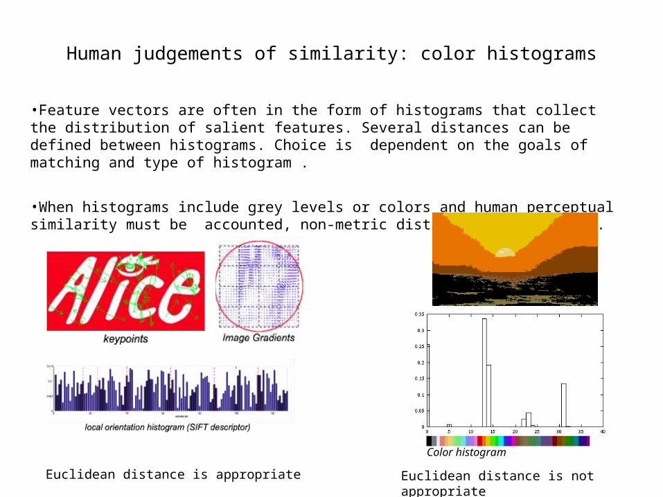
Human judgements of similarity: color histograms

•Feature vectors are often in the form of histograms that collect the distribution of salient features. Several distances can be defined between histograms. Choice is dependent on the goals of matching and type of histogram .

•When histograms include grey levels or colors and human perceptual similarity must be accounted, non-metric distances are preferred.

Color histogram

Euclidean distance is appropriate Euclidean distance is not appropriate

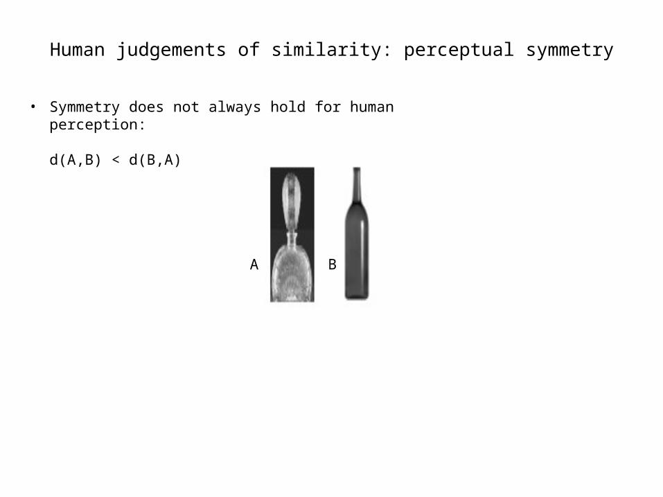
Human judgements of similarity: perceptual symmetry

• Symmetry does not always hold for human perception:

d(A,B) < d(B,A)

A B

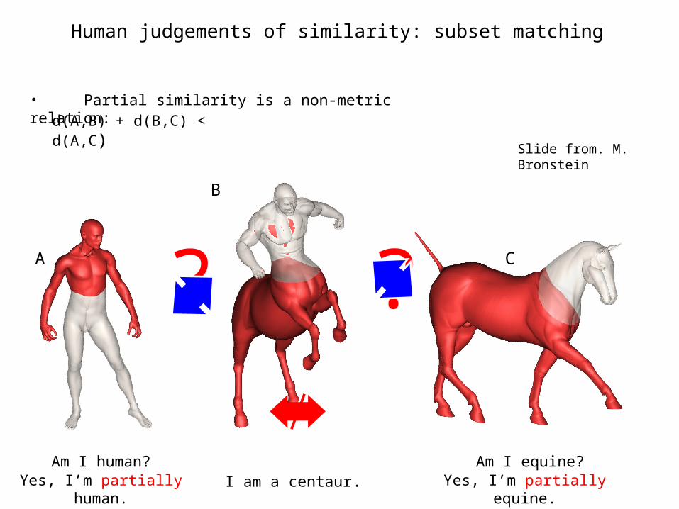
I am a centaur.Am I human? Am I equine?

Yes, I’m partially human. Yes, I’m partially equine.

• Partial similarity is a non-metric relation:

Human judgements of similarity: subset matching

A

B

C

d(A,B) + d(B,C) < d(A,C)

Slide from. M. Bronstein

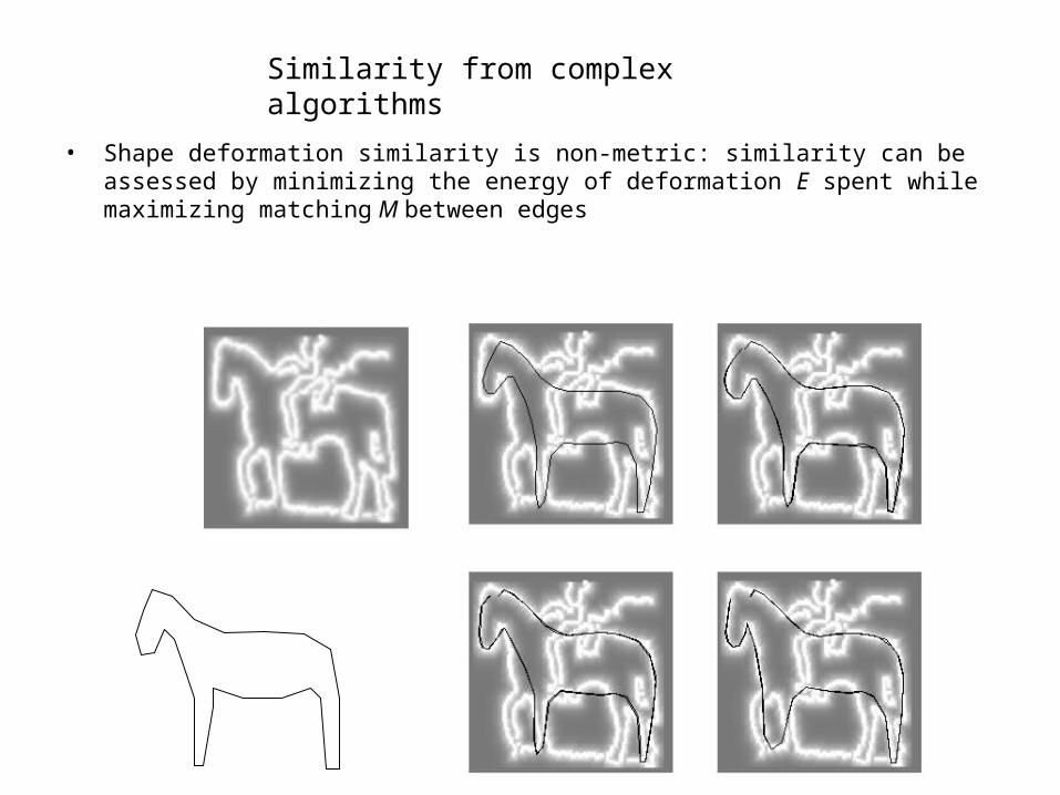
• Shape deformation similarity is non-metric: similarity can be assessed by minimizing the

energy of deformation E spent while maximizing matching M between edges

Similarity from complex algorithms

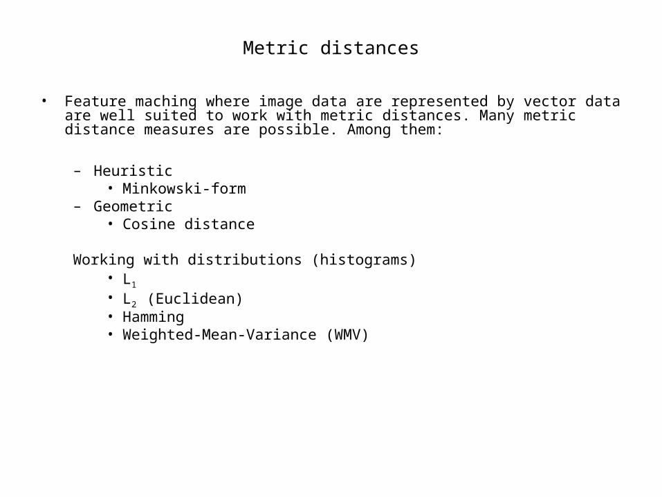
Metric distances

• Feature maching where image data are represented by vector data are well suited to work with metric distances. Many metric distance measures are possible. Among them:

– Heuristic• Minkowski-form

– Geometric • Cosine distance

Working with distributions (histograms)• L1• L2 (Euclidean)• Hamming• Weighted-Mean-Variance (WMV)

Minkowski distance

• Lp metrics also called Minkowski distance defined for two feature vectors A = (x1,…,xn) and B = (y1,…,yn) :

• L1: City Block or Manhattan d1 = ||A-B|| =

• L2: Euclidean distance (green line)

• L ∞: max, Chess board distance d∞ = maxi |xi – yi|

• The L1 norm and the L2 norm are mostly used because of their low computational cost.

L1 and L2 distance d(H1,H2)

L1 and L2 distance

• L1 and L2 distances are widely used in comparison of histogram representations. With color histograms comparison with Manhattan or Euclidean distance must take care of:− the L1 and Euclidean distances result in many false negatives because neighboring bins are not considered− the L2 distance is only suited for Lab and Luv color spaces.

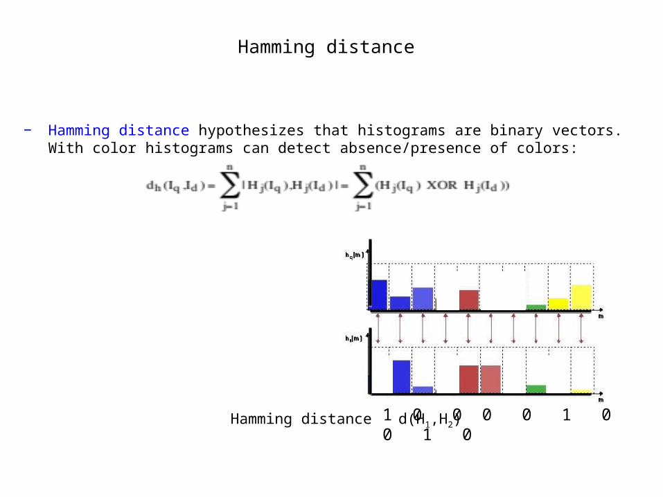
− Hamming distance hypothesizes that histograms are binary vectors. With color histograms can

detect absence/presence of colors:

Hamming distance d(H1,H2)

Hamming distance

1 0 0 0 0 1 0 0 1 0

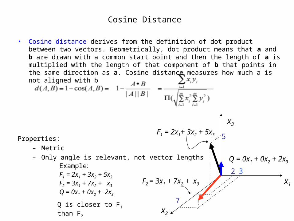
Cosine Distance

• Cosine distance derives from the definition of dot product between two vectors. Geometrically, dot product means that a and b are drawn with a common start point and then the length of a is multiplied with the length of that component of b that points in the same direction as a. Cosine distance measures how much a is not aligned with b

Properties:– Metric – Only angle is relevant, not vector lengths

Example:F1 = 2x1 + 3x2 + 5x3

F2 = 3x1 + 7x2 + x3

Q = 0x1 + 0x2 + 2x3

x3

x1

x2

F1 = 2x1+ 3x2 + 5x3

F2 = 3x1 + 7x2 + x3

Q = 0x1 + 0x2 + 2x3

7

32

5

Q is closer to F1 than F2

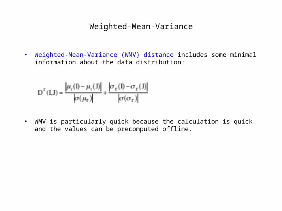
Weighted-Mean-Variance

• Weighted-Mean-Variance (WMV) distance includes some minimal information about the data distribution:

• WMV is particularly quick because the calculation is quick and the values can be precomputed offline.

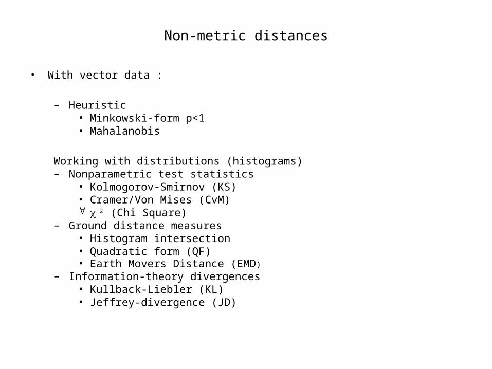
Non-metric distances

• With vector data :

– Heuristic• Minkowski-form p<1• Mahalanobis

Working with distributions (histograms)– Nonparametric test statistics

• Kolmogorov-Smirnov (KS)• Cramer/Von Mises (CvM) 2 (Chi Square)

– Ground distance measures• Histogram intersection• Quadratic form (QF)• Earth Movers Distance (EMD)

– Information-theory divergences• Kullback-Liebler (KL)• Jeffrey-divergence (JD)

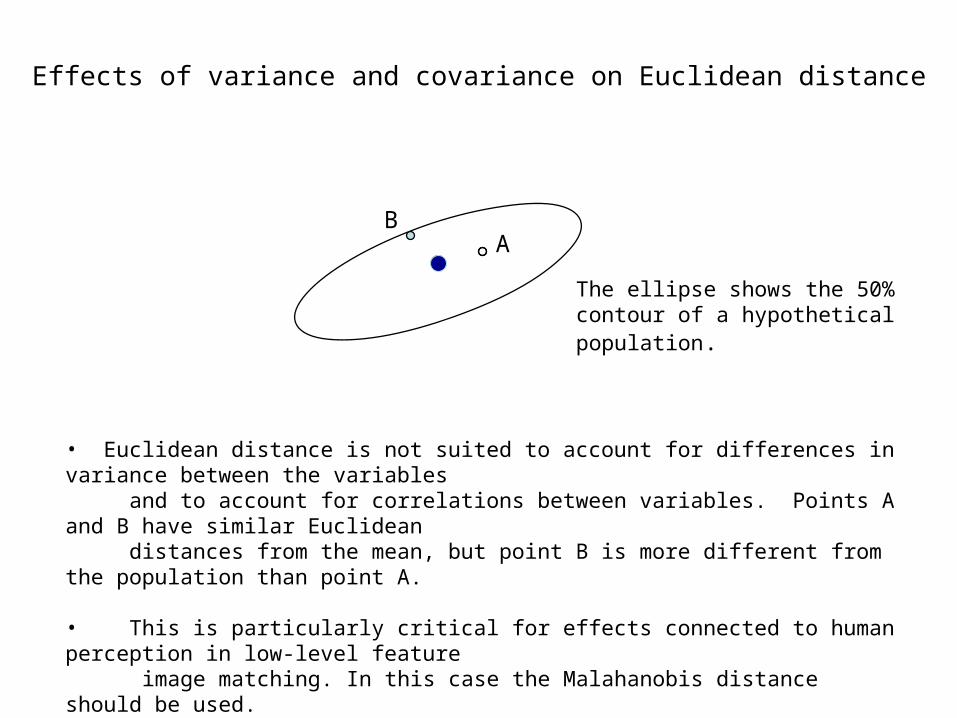
Effects of variance and covariance on Euclidean distance

• Euclidean distance is not suited to account for differences in variance between the variables and to account for correlations between variables. Points A and B have similar Euclidean distances from the mean, but point B is more different from the population than point A.

• This is particularly critical for effects connected to human perception in low-level feature image matching. In this case the Malahanobis distance should be used.

BA

The ellipse shows the 50% contour of a hypothetical population.

Mahalanobis (Quadratic) Distance

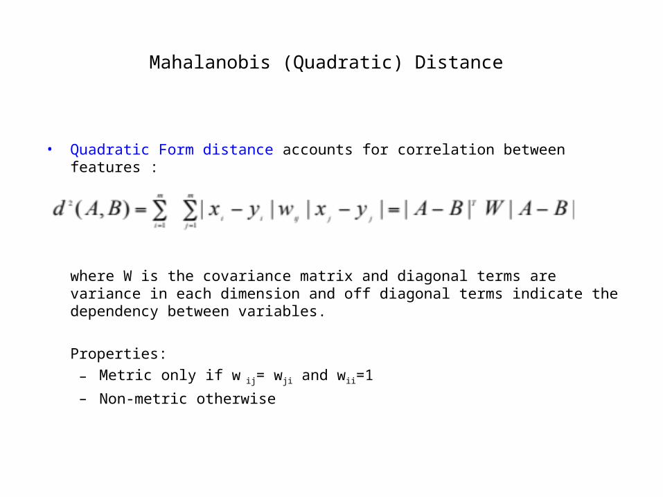
• Quadratic Form distance accounts for correlation between features :

where W is the covariance matrix and diagonal terms are variance in each dimension and off diagonal terms indicate the dependency between variables.

Properties:– Metric only if w ij= wji and wii=1 – Non-metric otherwise

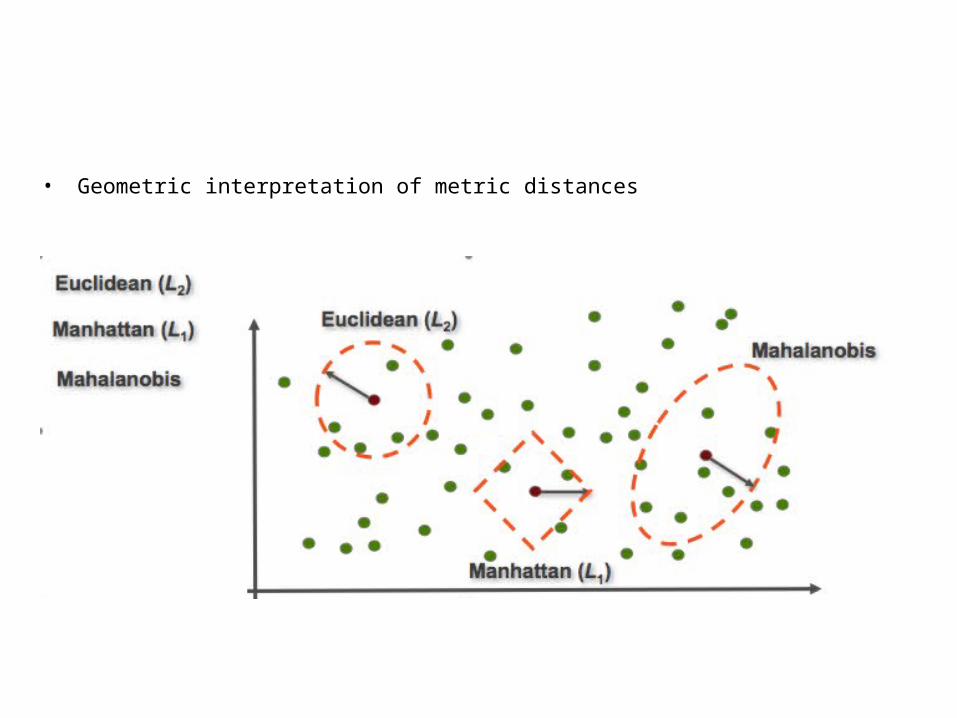
• Geometric interpretation of metric distances

• Mahanalobis distance is used for color histogram similarity as it closely resembles human perception:

being the similarity matrix denoting similarity between bins i and j

of N feature vectors x1,…,xN, each of length n.

• The quadratic form distance in image retrieval results in false positives because it tends to overestimate the mutual similarity of color distributions without a pronounced mode: the same mass in a given bin of the first histogram is simultaneously made to correspond to masses contained in different bins of the other histogram

Histogram intersection

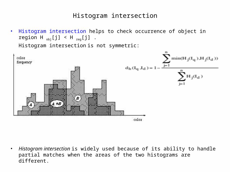
• Histogram intersection helps to check occurrence of object in region H obj[j] < H reg[j] .

Histogram intersection is not symmetric:

• Histogram intersection is widely used because of its ability to handle partial matches when the areas of the two histograms are different.

Cumulative Difference distances

• Kolmogorov-Smirnov distance (KS)

• Cramer/von Mises distance (CvM)

• Both Kolmogorov-Smirnov and Cramer/von Mises distance are statistical measures that measure the underlying similarity of two unbinned distributions. Work only for 1D data or cumulative histograms. They are non-symmetric distance functions.

where Fr(I; .) is the marginal histogram distribution

Cumulative Histogram

Normal Histogram Cumulative Histogram

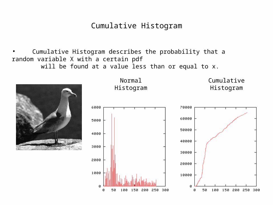
• Cumulative Histogram describes the probability that a random variable X with a certain pdf will be found at a value less than or equal to x.

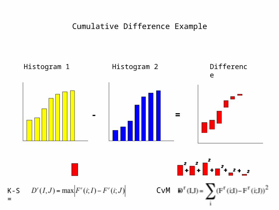
Cumulative Difference Example

Histogram 1 Histogram 2 Difference

- =

CvM =K-S =

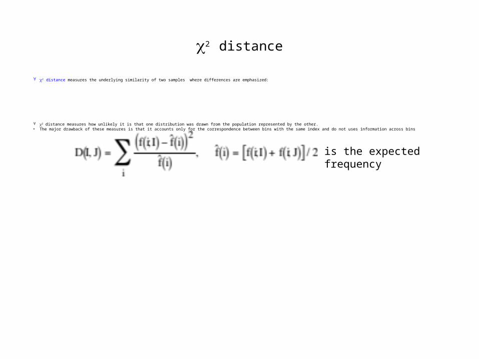
2 distance

2 distance measures the underlying similarity of two samples where differences are emphasized:

2 distance measures how unlikely it is that one distribution was drawn from the population represented by the other. • The major drawback of these measures is that it accounts only for the correspondence between bins with the same index and do not uses information across bins

is the expected frequency

Earth Mover’s distance

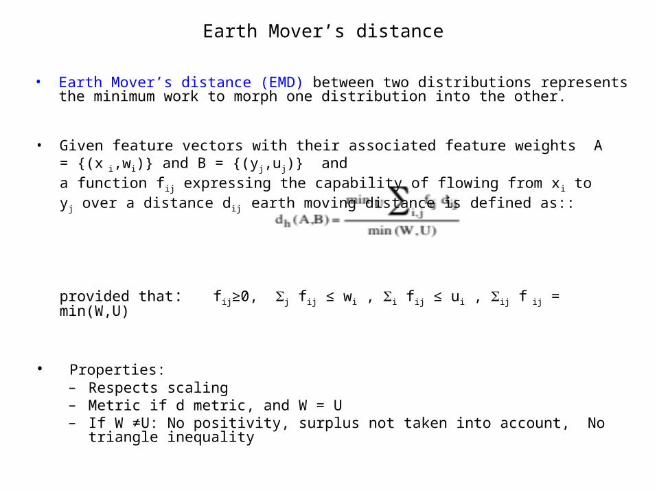
• Earth Mover’s distance (EMD) between two distributions represents the minimum work to morph one distribution into the other.

• Given feature vectors with their associated feature weights A = {(x i,wi)} and B = {(yj,uj)} and a function fij expressing the capability of flowing from xi to yj over a distance dij earth moving distance is defined as::

provided that: fij≥0, j fij ≤ wi , i fij ≤ ui , ij f ij = min(W,U)

• Properties:– Respects scaling – Metric if d metric, and W = U – If W ≠U: No positivity, surplus not taken into account, No triangle inequality

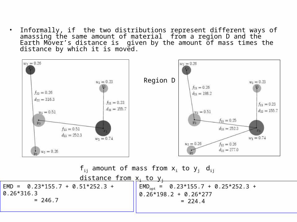
• Informally, if the two distributions represent different ways of amassing the same amount of material from a region D and the Earth Mover’s distance is given by the amount of mass times the distance by which it is moved.

Region D

EMD = 0.23*155.7 + 0.51*252.3 + 0.26*316.3 = 246.7

EMDopt = 0.23*155.7 + 0.25*252.3 + 0.26*198.2 + 0.26*277 = 224.4

fij amount of mass from xi to yj dij distance from xi to yj

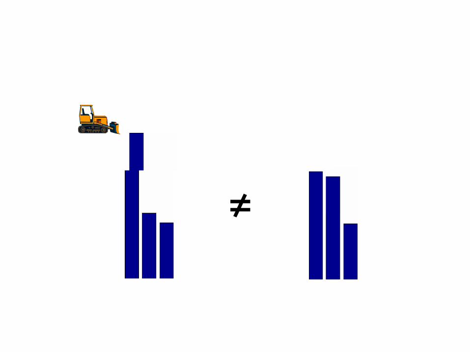
Earth Mover’s distance with histograms

≠

• Earth Mover’s distance is widely used for color, edge, motion vector histograms. It is the only measure that works on distributions with a different number of bins.

• However it has high computational cost. Considering two histograms H1and H2 as defined f.e. in a color space, pixels can be regarded as the unit of mass to be transported from one distribution to the other. It has to be based on some metric of distance between individual features.

≠

=

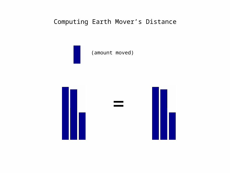
Computing Earth Mover’s Distance

=

(amount moved)

=

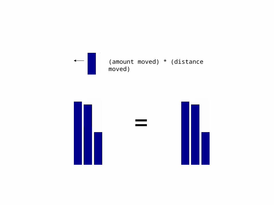
(amount moved) * (distance moved)

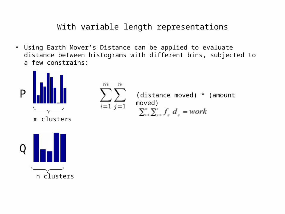
With variable length representations

m clusters

n clusters

P

Q

(distance moved) * (amount moved)

• Using Earth Mover’s Distance can be applied to evaluate distance between histograms with different bins, subjected to a few constrains:

Kullback-Leibler distance

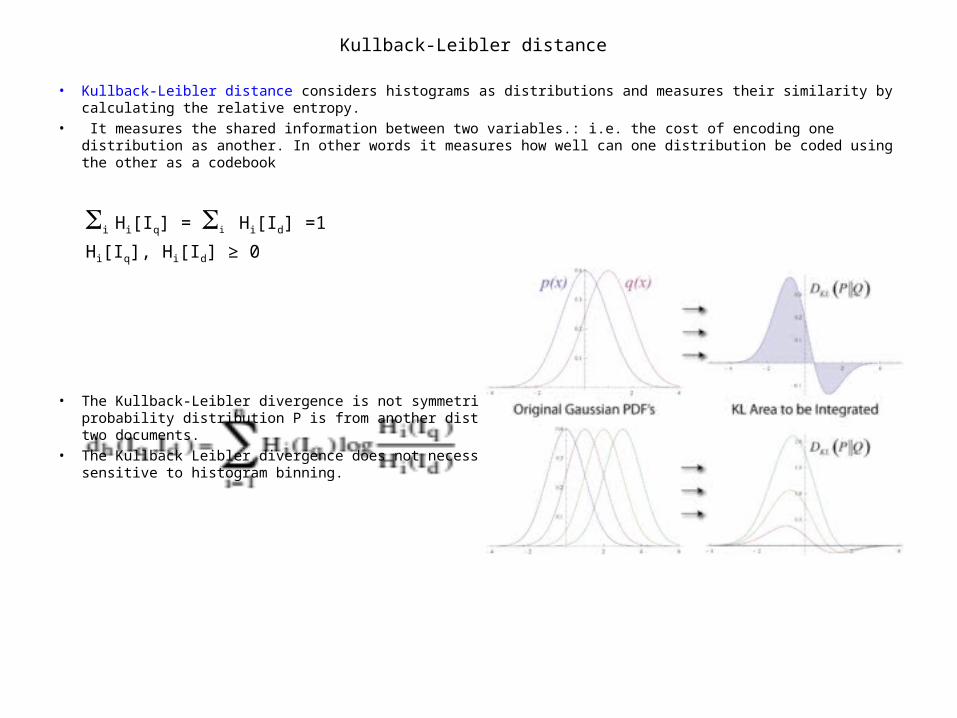
• Kullback-Leibler distance considers histograms as distributions and measures their similarity by calculating the relative entropy.

• It measures the shared information between two variables.: i.e. the cost of encoding one distribution as another. In other words it measures how well can one distribution be coded using the other as a codebook

i Hi[Iq] = iHi[Id] =1

Hi[Iq], Hi[Id] ≥ 0

• The Kullback-Leibler divergence is not symmetric. It can be used to determine “how far away” a probability distribution P is from another distribution Q i.e. as a distance measure between two documents.

• The Kullback Leibler divergence does not necessarily match perceptual similarity well and is sensitive to histogram binning.

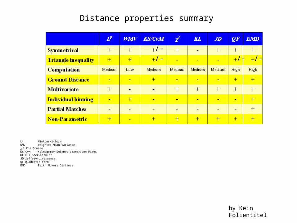
Distance properties summary

by Kein Folientitel

Lp Minkowski-formWMV Weighted-Mean-Variance 2 Chi SquareKS CvM Kolmogorov-Smirnov Cramer/von Mises KL Kullback-Liebler JD Jeffrey-divergence QF Quadratic formEMD Earth Movers Distance

/-/-/-

/-

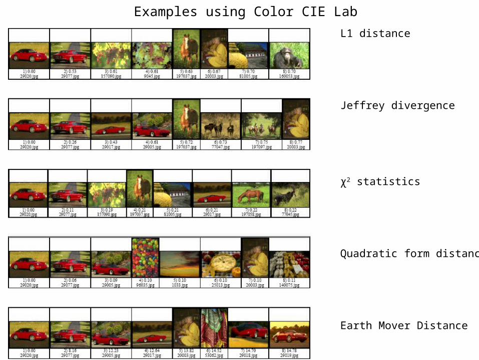
Using Color CIE Lab)L1 distance

Jeffrey divergence

χ2 statistics

Quadratic form distance

Earth Mover Distance

Examples using Color CIE Lab

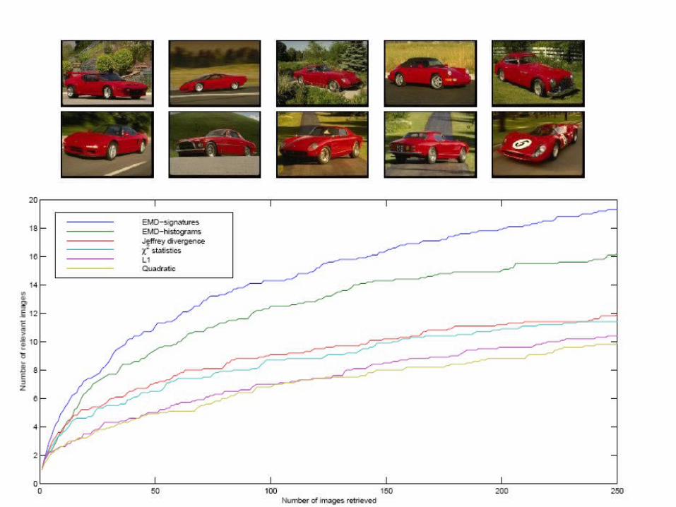
Image Lookup

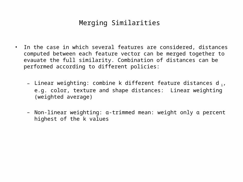
Merging Similarities

• In the case in which several features are considered, distances computed between each feature vector can be merged together to evauate the full similarity. Combination of distances can be performed according to different policies:

– Linear weighting: combine k different feature distances d i, e.g. color, texture and shape distances: Linear weighting (weighted average)

– Non-linear weighting: α-trimmed mean: weight only α percent highest of the k values

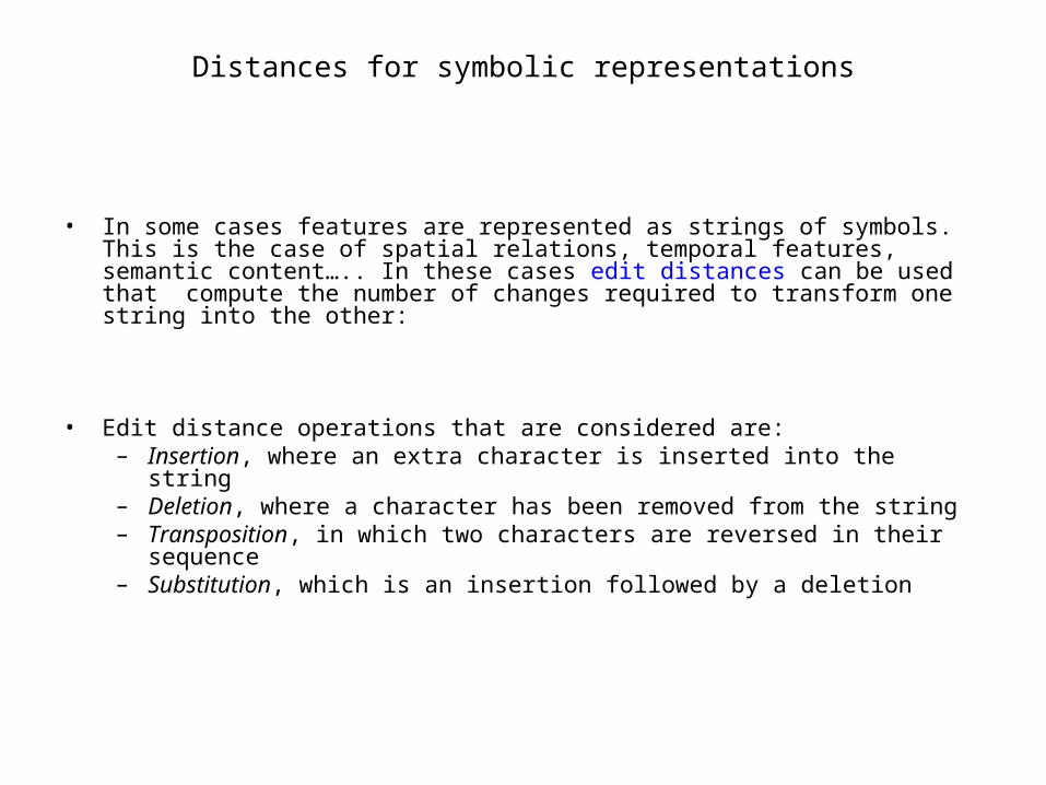
• In some cases features are represented as strings of symbols. This is the case of spatial

relations, temporal features, semantic content….. In these cases edit distances can be used that compute the number of changes required to transform one string into the other:

• Edit distance operations that are considered are:– Insertion, where an extra character is inserted into the string– Deletion, where a character has been removed from the string– Transposition, in which two characters are reversed in their sequence – Substitution, which is an insertion followed by a deletion

Distances for symbolic representations

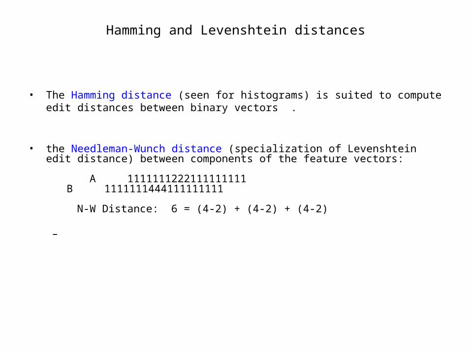
• The Hamming distance (seen for histograms) is suited to compute edit distances between binary vectors .

• the Needleman-Wunch distance (specialization of Levenshtein edit distance) between components of the feature vectors:

A 1111111222111111111B 1111111444111111111

N-W Distance: 6 = (4-2) + (4-2) + (4-2)

–

Hamming and Levenshtein distances