VISIBILITY FORECASTING FOR WARM AND COLD FOG … · project on warm and cold fog conditions and...
9
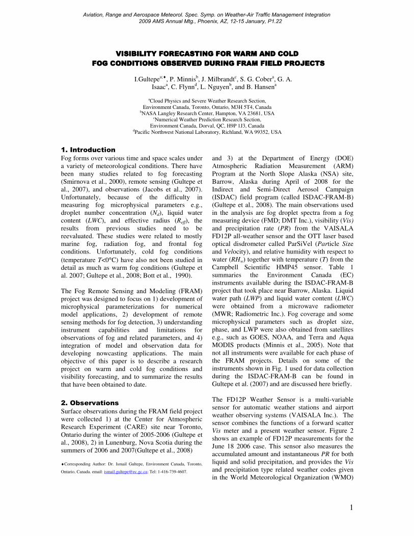
1 VISIBILITY FORECASTING FOR WARM AND COLD VISIBILITY FORECASTING FOR WARM AND COLD VISIBILITY FORECASTING FOR WARM AND COLD VISIBILITY FORECASTING FOR WARM AND COLD FOG CONDITIONS OBSERVED DURING FRAM FIELD PROJECTS FOG CONDITIONS OBSERVED DURING FRAM FIELD PROJECTS FOG CONDITIONS OBSERVED DURING FRAM FIELD PROJECTS FOG CONDITIONS OBSERVED DURING FRAM FIELD PROJECTS I.Gultepe a;♦ , P. Minnis b , J. Milbrandt c , S. G. Cober a , G. A. Isaac a , C. Flynn d , L. Nguyen b , and B. Hansen a a Cloud Physics and Severe Weather Research Section, Environment Canada, Toronto, Ontario, M3H 5T4, Canada b NASA Langley Research Center, Hampton, VA 23681,,USA c Numerical Weather Prediction Research Section, Environment Canada, Dorval, QC, H9P 1J3, Canada d Pacific Northwest National Laboratory, Richland, WA 99352, USA 1. Introduction Fog forms over various time and space scales under a variety of meteorological conditions. There have been many studies related to fog forecasting (Smirnova et al., 2000), remote sensing (Gultepe et al., 2007), and observations (Jacobs et al., 2007). Unfortunately, because of the difficulty in measuring fog microphysical parameters e.g., droplet number concentration (N d ), liquid water content (LWC), and effective radius (R eff ), the results from previous studies need to be reevaluated. These studies were related to mostly marine fog, radiation fog, and frontal fog conditions. Unfortunately, cold fog conditions (temperature T<0°C) have also not been studied in detail as much as warm fog conditions (Gultepe et al. 2007; Gultepe et al., 2008; Bott et al., 1990). The Fog Remote Sensing and Modeling (FRAM) project was designed to focus on 1) development of microphysical parameterizations for numerical model applications, 2) development of remote sensing methods for fog detection, 3) understanding instrument capabilities and limitations for observations of fog and related parameters, and 4) integration of model and observation data for developing nowcasting applications. The main objective of this paper is to describe a research project on warm and cold fog conditions and visibility forecasting, and to summarize the results that have been obtained to date. 2. Observations Surface observations during the FRAM field project were collected 1) at the Center for Atmospheric Research Experiment (CARE) site near Toronto, Ontario during the winter of 2005-2006 (Gultepe et al., 2008), 2) in Lunenburg, Nova Scotia during the summers of 2006 and 2007(Gultepe et al., 2008) ♦Corresponding Author: Dr. Ismail Gultepe, Environment Canada, Toronto, Ontario, Canada. email: [email protected] ; Tel: 1-416-739-4607. and 3) at the Department of Energy (DOE) Atmospheric Radiation Measurement (ARM) Program at the North Slope Alaska (NSA) site, Barrow, Alaska during April of 2008 for the Indirect and Semi-Direct Aerosol Campaign (ISDAC) field program (called ISDAC-FRAM-B) (Gultepe et al., 2008). The main observations used in the analysis are fog droplet spectra from a fog measuring device (FMD; DMT Inc.), visibility (Vis) and precipitation rate (PR) from the VAISALA FD12P all-weather sensor and the OTT laser based optical disdrometer called ParSiVel (Particle Size and Velocity), and relative humidity with respect to water (RH w ) together with temperature (T) from the Campbell Scientific HMP45 sensor. Table 1 summaries the Environment Canada (EC) instruments available during the ISDAC-FRAM-B project that took place near Barrow, Alaska. Liquid water path (LWP) and liquid water content (LWC) were obtained from a microwave radiometer (MWR; Radiometric Inc.). Fog coverage and some microphysical parameters such as droplet size, phase, and LWP were also obtained from satellites e.g., such as GOES, NOAA, and Terra and Aqua MODIS products (Minnis et al., 2005). Note that not all instruments were available for each phase of the FRAM projects. Details on some of the instruments shown in Fig. 1 used for data collection during the ISDAC-FRAM-B can be found in Gultepe et al. (2007) and are discussed here briefly. The FD12P Weather Sensor is a multi-variable sensor for automatic weather stations and airport weather observing systems (VAISALA Inc.). The sensor combines the functions of a forward scatter Vis meter and a present weather sensor. Figure 2 shows an example of FD12P measurements for the June 18 2006 case. This sensor also measures the accumulated amount and instantaneous PR for both liquid and solid precipitation, and provides the Vis and precipitation type related weather codes given in the World Meteorological Organization (WMO) Aviation, Range and Aerospace Meteorol. Spec. Symp. on Weather-Air Traffic Management Integration 2009 AMS Annual Mtg., Phoenix, AZ, 12-15 January, P1.22
Transcript of VISIBILITY FORECASTING FOR WARM AND COLD FOG … · project on warm and cold fog conditions and...
1
VISIBILITY FORECASTING FOR WARM AND COLDVISIBILITY FORECASTING FOR WARM AND COLDVISIBILITY FORECASTING FOR WARM AND COLDVISIBILITY FORECASTING FOR WARM AND COLD
FOG CONDITIONS OBSERVED DURING FRAM FIELD PROJECTS FOG CONDITIONS OBSERVED DURING FRAM FIELD PROJECTS FOG CONDITIONS OBSERVED DURING FRAM FIELD PROJECTS FOG CONDITIONS OBSERVED DURING FRAM FIELD PROJECTS
I.Gultepea;♦
, P. Minnisb, J. Milbrandt
c, S. G. Cober
a, G. A.
Isaaca, C. Flynn
d, L. Nguyen
b, and B. Hansen
a
aCloud Physics and Severe Weather Research Section,
Environment Canada, Toronto, Ontario, M3H 5T4, Canada bNASA Langley Research Center, Hampton, VA 23681,,USA
cNumerical Weather Prediction Research Section,
Environment Canada, Dorval, QC, H9P 1J3, Canada dPacific Northwest National Laboratory, Richland, WA 99352, USA
1. Introduction
Fog forms over various time and space scales under
a variety of meteorological conditions. There have
been many studies related to fog forecasting
(Smirnova et al., 2000), remote sensing (Gultepe et
al., 2007), and observations (Jacobs et al., 2007).
Unfortunately, because of the difficulty in
measuring fog microphysical parameters e.g.,
droplet number concentration (Nd), liquid water
content (LWC), and effective radius (Reff), the
results from previous studies need to be
reevaluated. These studies were related to mostly
marine fog, radiation fog, and frontal fog
conditions. Unfortunately, cold fog conditions
(temperature T<0°C) have also not been studied in
detail as much as warm fog conditions (Gultepe et
al. 2007; Gultepe et al., 2008; Bott et al., 1990).
The Fog Remote Sensing and Modeling (FRAM)
project was designed to focus on 1) development of
microphysical parameterizations for numerical
model applications, 2) development of remote
sensing methods for fog detection, 3) understanding
instrument capabilities and limitations for
observations of fog and related parameters, and 4)
integration of model and observation data for
developing nowcasting applications. The main
objective of this paper is to describe a research
project on warm and cold fog conditions and
visibility forecasting, and to summarize the results
that have been obtained to date.
2. Observations
Surface observations during the FRAM field project
were collected 1) at the Center for Atmospheric
Research Experiment (CARE) site near Toronto,
Ontario during the winter of 2005-2006 (Gultepe et
al., 2008), 2) in Lunenburg, Nova Scotia during the
summers of 2006 and 2007(Gultepe et al., 2008)
♦Corresponding Author: Dr. Ismail Gultepe, Environment Canada, Toronto,
Ontario, Canada. email: [email protected]; Tel: 1-416-739-4607.
and 3) at the Department of Energy (DOE)
Atmospheric Radiation Measurement (ARM)
Program at the North Slope Alaska (NSA) site,
Barrow, Alaska during April of 2008 for the
Indirect and Semi-Direct Aerosol Campaign
(ISDAC) field program (called ISDAC-FRAM-B)
(Gultepe et al., 2008). The main observations used
in the analysis are fog droplet spectra from a fog
measuring device (FMD; DMT Inc.), visibility (Vis)
and precipitation rate (PR) from the VAISALA
FD12P all-weather sensor and the OTT laser based
optical disdrometer called ParSiVel (Particle Size
and Velocity), and relative humidity with respect to
water (RHw) together with temperature (T) from the
Campbell Scientific HMP45 sensor. Table 1
summaries the Environment Canada (EC)
instruments available during the ISDAC-FRAM-B
project that took place near Barrow, Alaska. Liquid
water path (LWP) and liquid water content (LWC)
were obtained from a microwave radiometer
(MWR; Radiometric Inc.). Fog coverage and some
microphysical parameters such as droplet size,
phase, and LWP were also obtained from satellites
e.g., such as GOES, NOAA, and Terra and Aqua
MODIS products (Minnis et al., 2005). Note that
not all instruments were available for each phase of
the FRAM projects. Details on some of the
instruments shown in Fig. 1 used for data collection
during the ISDAC-FRAM-B can be found in
Gultepe et al. (2007) and are discussed here briefly.
The FD12P Weather Sensor is a multi-variable
sensor for automatic weather stations and airport
weather observing systems (VAISALA Inc.). The
sensor combines the functions of a forward scatter
Vis meter and a present weather sensor. Figure 2
shows an example of FD12P measurements for the
June 18 2006 case. This sensor also measures the
accumulated amount and instantaneous PR for both
liquid and solid precipitation, and provides the Vis
and precipitation type related weather codes given
in the World Meteorological Organization (WMO)
Aviation, Range and Aerospace Meteorol. Spec. Symp. on Weather-Air Traffic Management Integration 2009 AMS Annual Mtg., Phoenix, AZ, 12-15 January, P1.22
2
standard SYNOP and METAR messages. The
FD12P detects precipitation droplets from rapid
changes in the scatter signal. Based on the
manufacturer’s specifications, the accuracy of the
FD12P measurements for Vis and PR are
approximately 10% and 0.05 mm h-1
respectively.
The fog-related microphysics parameters e.g. LWC,
size, and droplet number concentration (Nd) were
calculated from the FMD spectra for both liquid
and ice clouds. Although an ice particle counter
was available, its measurement size range is likely
beyond the upper limit of the typical fog particle
size, e.g., 50 µm. For subsaturated conditions, the
Climatronics Aerosol Profiling (CAP) probe was
used for measuring aerosol size and spectra
between 0.3 and 10 µm. In saturated conditions,
CAP measures the nucleated particles’
characteristics.
The NOAA AVHRR (and/or GOES) observations
were also available during FRAM projects, and
some retrieval methods were used to detect fog
conditions and its microphysics.
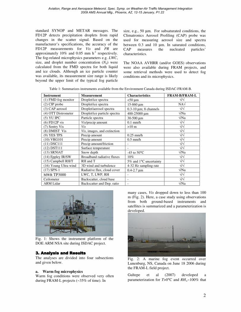
Table 1: Summarizes instruments available from the Environment Canada during ISDAC-FRAM-B.
Fig. 1: Shows the instrument platform of the
DOE ARM NSA site during ISDAC project.
3. Analysis3. Analysis3. Analysis3. Analysis a a a and Resultsnd Resultsnd Resultsnd Results
The analyses are divided into four subsections
and given below.
a. Warm fog microphysics Warm fog conditions were observed very often
during FRAM-L projects (~35% of time). In
many cases, Vis dropped down to less than 100
m (Fig. 2). Here, a case study using observations
from both ground-based instruments and
satellites is summarized and a parameterization is
developed.
Fig. 2: A marine fog event occurred over
Lunenburg, NS, Canada on June 18 2006 during
the FRAM-L field project.
Gultepe et al
(2007) developed a
parameterization for T>0°C and RHw~100% that
Instrument Measurement Characteristics FRAM-B/FRAM-L
(1) FMD fog monitor Droplet/ice spectra <50 µm √/√
(2) CIP probe Droplet/ice spectra 15-860 µm NA√
(3) CAP aerosol Droplet/aerosol spectra 0.3-10 µm; 8 channels √/√
(4) OTT Distrometer Droplet/ice particle spectra 400-25000 µm √/Na
(5) YU IPC Particle spectra 30-500 µm √/Na
(6) FD12P vis Vis/precip amount 0.1 mm/h √/√
(7) Sentry Vis Vis >10 m √/√
(8) DMIST Vis Vis, images, and extinction √/√
(9) YES TPS Precip amount 0.25 mm/h √/√
(10) VRG101 Precip amount 0.5 mm/h √/√
(11) DSC111 Precip amount/friction - √/√
(12) DST111 Surface temperature - √/√
(13) SR50AT Snow depth -45 to 50°C √/Na
(14) Eppley IR/SW Broadband radiative fluxes 10% √/√
(15) Campbell RH/T RH and T 5% and 1°C uncertainty √/√
(16) Young Ultra wind 3D wind and turbulence 4-32 Hz sampling rate √/√
(17) SPN-1 Radiative flux, cloud cover 0.4-2.7 µm √/Na
MWR TP3000 LWC, T, LWP, RH - √/√
Ceilometer Backscatter, cloud base - √/√
ARM Lidar Backscatter and Dep. ratio - √/Na
Aviation, Range and Aerospace Meteorol. Spec. Symp. on Weather-Air Traffic Management Integration 2009 AMS Annual Mtg., Phoenix, AZ, 12-15 January, P1.22
3
is based on liquid water content (LWC) and
droplet number concentration (Nd). The US
current Rapid Update Cycle (RUC) model uses a
Vis-LWC relationship for fog visibility
(Smirnova et al. 2000; Stoelinga and Warner,
1999). Using information that Vis decreases with
increasing Nd and LWC, a relationship between
Visobs and (LWC.Nd)-1
called the “fog index” is
determined as
6473.0)(
002.1
d
obsNLWC
Vis⋅
= . (1)
This fit suggests that Vis is inversely related to
both LWC and Nd.. The maximum limiting LWC
and Nd values used in the derivation of (1) are
about 400 cm-3
and 0.5 g m-3
, respectively. The
minimum limiting Nd and LWC values are 1 cm-3
and 0.005 g m-3
, respectively. In (1), Nd can be
fixed as 100 cm-3
for marine environments and
200 cm-3
for continental fog conditions. These
values of Nd,, which were traditionally used in
modeling applications, cannot be valid for all
environmental conditions (Gultepe and Isaac,
2004). Examples of the fog microphysical
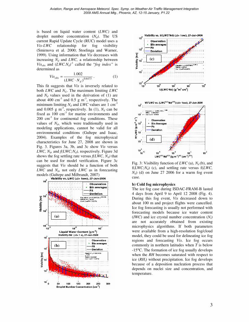
characteristics for June 27, 2008 are shown in
Fig. 3. Figures 3a, 3b, and 3c show Vis versus
LWC, Nd, and f(LWC;Nd), respectively. Figure 3d
shows the fog settling rate versus f(LWC, Nd) that
can be used for model verification. Figure 3c
suggests that Vis should be a function of both
LWC and Nd, not only LWC as in forecasting
models (Gultepe and Milbrandt, 2007)
Fig. 3: Visibility function of LWC (a), Nd (b), and
f(LWC;Nd) (c), and settling rate versus f(LWC,
Nd) (d) on June 27 2006 for a warm fog event
case.
b) Cold fog microphysics The ice fog case during ISDAC-FRAM-B lasted
4 days from April 9 to April 12 2008 (Fig. 4).
During this fog event, Vis decreased down to
about 100 m and project flights were cancelled.
Ice fog forecasting is usually not performed with
forecasting models because ice water content
(IWC) and ice crystal number concentration (Ni)
are not accurately obtained from existing
microphysics algorithms. If both parameters
were available from a high-resolution fog/cloud
model, they could be used for delineating ice fog
regions and forecasting Vis. Ice fog occurs
commonly in northern latitudes when T is below
-15°C. The formation of ice fog usually develops
when the RH becomes saturated with respect to
ice (RHi) without precipitation. Ice fog develops
because of a deposition nucleation process that
depends on nuclei size and concentration, and
temperature.
(a)
(c)
(d)
(b)
Aviation, Range and Aerospace Meteorol. Spec. Symp. on Weather-Air Traffic Management Integration 2009 AMS Annual Mtg., Phoenix, AZ, 12-15 January, P1.22
4
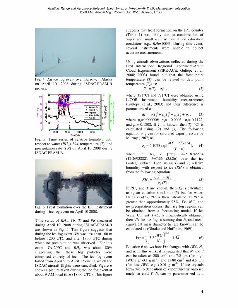
Fig. 4: An ice fog event over Barrow, Alaska
on April 10, 2008 during ISDAC-FRAM-B
project.
Fig. 5: Time series of relative humidity with
respect to water (RHw), Vis, temperature (T), and
precipitation rate (PR) on April 10 2008 during
ISDAC-FRAM-B.
Fig. 6: Frost formation over the IPC instrument
during ice fog event on April 10 2008.
Time series of RHw, Vis, T, and PR measured
during April 10, 2008 during ISDAC-FRAM-B
are shown in Fig. 5. This figure suggests that
during the ice fog event, Vis was less than 100 m
before 1200 UTC and after 1800 UTC during
which no precipitation was observed. For this
event, T<-20°C and RHw was about 80%
suggesting that these fog particles were
composed entirely of ice. The ice fog event
lasted from April 9 to April 12 during which the
ISDAC aircraft flights were cancelled. Figure 6
shows a picture taken during the ice fog event at
about 9 AM local time (18:00 UTC). This figure
suggests that frost formation on the IPC counter
(Table 1) was likely due to condensation of
vapor and small ice particles at ice saturation
conditions e.g., RHi=100%. During this event,
several instruments were unable to collect
accurate measurements.
Using aircraft observations collected during the
First International Regional Experiment-Arctic
Cloud Experiment (FIRE-ACE; Gultepe et al.
2008; 2003) found out that the frost point
temperature (Tf) can be related to dew point
temperature (Td) as:
fTT df ∆+= , (2)
where Td [°C] and Tf [°C] were obtained using
LiCOR instrument humidity measurements
(Gultepe et al., 2003) and their difference is
parameterized as:
41
32
23
1 pTpTpTpf ddd +++=∆ , (3)
where p1=0.000006; p2= -0.0003; p3=-0.1122;
and p4= 0.1802. If Td is known, then Tf [°C] is
calculated using. (2) and (3). The following
equation is given for saturated vapor pressure by
Murray (1967) as
])(
)16.273(exp[1078.6
bT
Taes
−
−= , (4)
where T [K], e [mb], a=21.8745584
(17.2693882); b=7.66 (35.86) over the ice
(water) surface. Then, using Tf and T, relative
humidity with respect to ice (RHi) is obtained
from the following equation
)(
)(
Te
fTeRH
si
dii
∆+= . (5)
If RHw and T are known, then Td is calculated
using an equation similar to (5) but for water.
Using (2)-(5), RHi is then calculated. If RHi is
greater than approximately 95%, T<-10°C, and
no precipitation occurs, then ice fog regions can
be obtained from a forecasting model. If Ice
Water Content (IWC) is prognostically obtained,
then Vis for ice fog, assuming that Ni and mean
equivalent mass diameter (d) are known, can be
calculated as (Ohtake and Huffman, 1969):
dN
IWCVis
i
5.12.33
13/1
−
= . (6)
Equation 6 shows how Vis changes with IWC, Ni,
and d. In this work, it is suggested that Ni and d
can be taken as 200 cm-3
and 7.2 µm (for high
IWC e.g.>0.1 g m-3
), and as 80 cm-3
and 4.5 µm
(for low IWC, e.g.,>0.01 g m-3
). If ice crystals
form due to deposition of vapor directly onto ice
nuclei at cold T, Ni can be parameterized as a
Aviation, Range and Aerospace Meteorol. Spec. Symp. on Weather-Air Traffic Management Integration 2009 AMS Annual Mtg., Phoenix, AZ, 12-15 January, P1.22
5
function of RHi. A relationship between Ni and
RHi for ice fog has not been demonstrated. Note
that (6) needs to be verified using measurements
from the ISDAC-FRAM-B project. Preliminary
results using FRAM-B observations as shown in
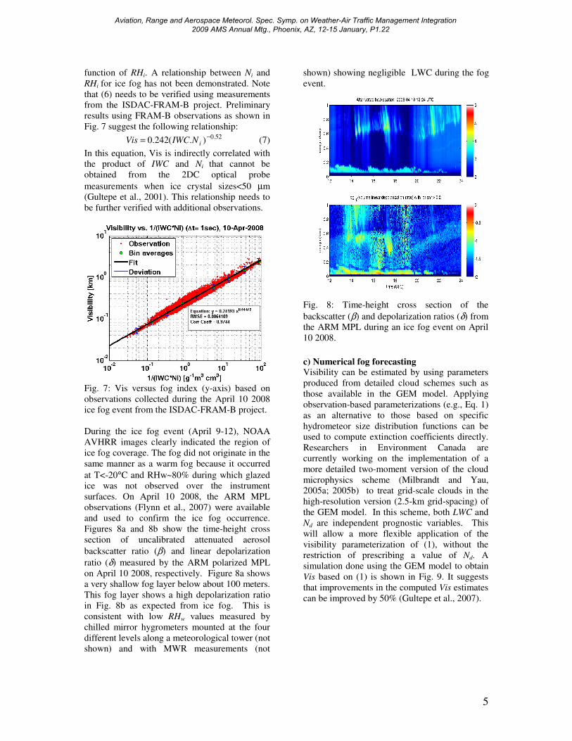
Fig. 7 suggest the following relationship: 52.0).(242.0 −= iNIWCVis (7)
In this equation, Vis is indirectly correlated with
the product of IWC and Ni that cannot be
obtained from the 2DC optical probe
measurements when ice crystal sizes<50 µm
(Gultepe et al., 2001). This relationship needs to
be further verified with additional observations.
Fig. 7: Vis versus fog index (y-axis) based on
observations collected during the April 10 2008
ice fog event from the ISDAC-FRAM-B project.
During the ice fog event (April 9-12), NOAA
AVHRR images clearly indicated the region of
ice fog coverage. The fog did not originate in the
same manner as a warm fog because it occurred
at T<-20°C and RHw~80% during which glazed
ice was not observed over the instrument
surfaces. On April 10 2008, the ARM MPL
observations (Flynn et al., 2007) were available
and used to confirm the ice fog occurrence.
Figures 8a and 8b show the time-height cross
section of uncalibrated attenuated aerosol
backscatter ratio (β) and linear depolarization
ratio (δ) measured by the ARM polarized MPL
on April 10 2008, respectively. Figure 8a shows
a very shallow fog layer below about 100 meters.
This fog layer shows a high depolarization ratio
in Fig. 8b as expected from ice fog. This is
consistent with low RHw values measured by
chilled mirror hygrometers mounted at the four
different levels along a meteorological tower (not
shown) and with MWR measurements (not
shown) showing negligible LWC during the fog
event.
Fig. 8: Time-height cross section of the
backscatter (β) and depolarization ratios (δ) from
the ARM MPL during an ice fog event on April
10 2008.
c) Numerical fog forecasting Visibility can be estimated by using parameters
produced from detailed cloud schemes such as
those available in the GEM model. Applying
observation-based parameterizations (e.g., Eq. 1)
as an alternative to those based on specific
hydrometeor size distribution functions can be
used to compute extinction coefficients directly.
Researchers in Environment Canada are
currently working on the implementation of a
more detailed two-moment version of the cloud
microphysics scheme (Milbrandt and Yau,
2005a; 2005b) to treat grid-scale clouds in the
high-resolution version (2.5-km grid-spacing) of
the GEM model. In this scheme, both LWC and
Nd are independent prognostic variables. This
will allow a more flexible application of the
visibility parameterization of (1), without the
restriction of prescribing a value of Nd. A
simulation done using the GEM model to obtain
Vis based on (1) is shown in Fig. 9. It suggests
that improvements in the computed Vis estimates
can be improved by 50% (Gultepe et al., 2007).
Aviation, Range and Aerospace Meteorol. Spec. Symp. on Weather-Air Traffic Management Integration 2009 AMS Annual Mtg., Phoenix, AZ, 12-15 January, P1.22
6
Fig. 9: Simulated warm fog event using (1) and
a double moment microphysical scheme on June
27 2006. It was obtained using a GEM
simulation based on a 14 hr forecast valid at
0600 UTC.
d) Satellite retrievals
The remote sensing study of the June 27 warm
fog case is performed using 1) Terra MODIS
satellite retrievals and 2) GOES and GEM model
output work (Gultepe et al., 2007). The retrieval
results suggest that integration of satellite
observations with model output improved fog
forecasting. The Reff obtained from the MODIS
observations of ~7 µm over the project site (not
shown) were found to be comparable with the
FMD measurements (Fig. 10) where median
value of Reff is estimated to be 6-8 µm. Figure 11
shows the warm fog area as detected using the
integration of GOES observations and GEM
model output. In this image, the model-based
surface temperature and screen level RH were
used in the integration of satellite observations.
Gultepe et al. (2007) showed that inclusion of
model output in the fog analysis together with
satellite observations improved fog detection up
to 30% of time.
During the April 10 2008 ice fog case, the
NOAA AVHRR RGB image (Fig. 12) showed
that ice fog covered a large area over the
northern Alaska and Canada. It is optically thin
as evident from the visibility of surface features
underneath it. The ice fog conditions at the NSA
site were characterized using surface
observations. In this case, IWC reached to 0.2 g
m-3
and Vis was less than about 100 m. Further
analysis of this case using the retrieval
techniques will help us to better detect the ice
fog conditions in the northern latitudes.
Fig. 10: Effective size (Reff) versus LWC
obtained from FMD measurements on June 27
2006.
Fig. 11: A fog region obtained using GOES
observations and GEM model output on June 27
2006.
Fig. 12: The NOAA AVHRR RGB image of the
ice fog event that occurred on April 10 2008 over
the Barrow, Alaska. Ice fog regions are shown
by light blue color.
5. Discussion
To accurately forecast/nowcast fog Vis, accurate
model output parameters are required, e.g., LWC,
Aviation, Range and Aerospace Meteorol. Spec. Symp. on Weather-Air Traffic Management Integration 2009 AMS Annual Mtg., Phoenix, AZ, 12-15 January, P1.22
7
Nd, RH, and PR. If model output values for rain,
snow, RH, and LWC are not accurate to better
than 20-30%, the uncertainty in Vis can be more
than 50% (Gultepe et al., 2006). If fog LWC and
Nd are not accurately known from a model at the
levels closest to the surface, then Vis based on
other parameters e.g., such as PR or RH, or both,
cannot be used to obtain accurate Vis values. Fog
LWC (or IWC) and Nd (or Ni) are the major
factors required for accurate Vis calculations and
they should be obtained to an accuracy of about
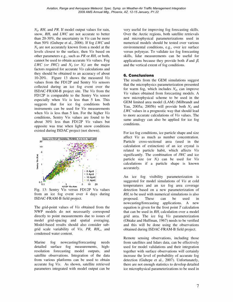
10-20%. Figure 13 shows the measured Vis
values from the FD12P and Sentry Vis sensors
collected during an ice fog event over the
ISDAC-FRAM-B project site. The Vis from the
FD12P is comparable to the Sentry Vis sensor
especially when Vis is less than 5 km. This
suggests that for ice fog conditions both
instruments can be used for Vis measurements
when Vis is less than 5 km. For the higher Vis
conditions, Sentry Vis values are found to be
about 30% less than FD12P Vis values but
opposite was true when light snow conditions
existed during ISDAC project (not shown).
Fig. 13: Sentry Vis versus FD12P Vis values
from an ice fog event over 4 days during
ISDAC-FRAM-B field project.
The grid-point values of Vis obtained from the
NWP models do not necessarily correspond
directly to point measurements due to issues of
model grid-spacing and spatial averaging.
Model-based results should also consider sub-
grid scale variability of Vis, PR, RHw, and
condensed water content.
Marine fog nowcasting/forecasting needs
detailed surface fog measurements, high-
resolution forecasting model outputs, and
satellite observations. Integration of the data
from various platforms can be used to obtain
accurate fog Vis. As shown, satellite retrieved
parameters integrated with model output can be
very useful for improving fog forecasting skills.
Over the Arctic regions, both satellite retrievals
and microphysical parameterizations used in
numerical models should be tested over various
environmental conditions, e.g., over ice surface
versus polynyas. To validate ice fog forecasting
skills, lidar measurements can be useful for
applications because they provide both δ and β,
and the vertical extent of fog conditions.
6. Conclusions
The results from the GEM simulations suggest
that the microphysics parameterization presented
for warm fog, which includes Nd, can improve
Vis values obtained from forecasting models. A
new microphysical scheme to be used in the
GEM limited area model (LAM) (Milbrandt and
Yau, 2005a; 2005b) will provide both Nd and
LWC values in a prognostic way that should lead
to more accurate calculations of Vis values. The
same analogy can also be applied for ice fog
conditions.
For ice fog conditions, ice particle shape and size
affect Vis as much as number concentration.
Particle cross-sectional area (used in the
calculation of extinction) of an ice crystal is
related to particle habit, which affects Vis
significantly. The combination of IWC and ice
particle size (or Ni) can be used for Vis
calculations if a particle shape is known
accurately.
An ice fog visibility parameterization is
suggested for model simulations of Vis at cold
temperatures and an ice fog area coverage
detection based on a new parameterization of
RHi to be used with numerical simulations is also
proposed. These can be used in
nowcasting/forecasting applications. A new
equation is given for the frost point T calculation
that can be used in RHi calculation over a model
grid area. The ice fog Vis parameterization
(Ohtake and Huffman, 1967) needs to be verified
and this will be done using the observations
obtained during ISDAC-FRAM-B field project.
Remote sensing observations, including those
from satellites and lidars data, can be effectively
used for model validations and their integration
together with surface observations will certainly
increase the level of probability of accurate fog
detection (Gultepe et al., 2007). Unfortunately,
there are not enough statistics to develop detailed
ice microphysical parameterizations to be used in
Aviation, Range and Aerospace Meteorol. Spec. Symp. on Weather-Air Traffic Management Integration 2009 AMS Annual Mtg., Phoenix, AZ, 12-15 January, P1.22
8
forecasting applications but a future ice fog
project in Arctic will be performed to improve
the data quality in ice fog conditions.
ACKNOWLEDGEMENTSACKNOWLEDGEMENTSACKNOWLEDGEMENTSACKNOWLEDGEMENTS
Funding for the FRAM project was provided by
the Canadian National Search and Rescue
Secretariat and Environment Canada. The
authors are thankful to M. Wasey and R. Reed of
Environment Canada for technical support.
ISDAC was supported by the Office of
Biological and Environmental Research of the
U.S. Department of Energy through the
Atmospheric Radiation Measurement (ARM)
program and the ARM Aerial Vehicle Program
with contributions from the DOE Atmospheric
Sciences Program (ASP), Environment Canada
and the National Research Council of Canada.
Data were obtained from the ARM program
archive, sponsored by the U.S. DOE, Office of
Science, Office of Biological and Environmental
Research, Environmental Sciences Division. The
satellite analyses were supported by the ARM
program and the NASA Advanced Satellite
Aviation-weather Products (ASAP) Program.
REFERREFERREFERREFERENCESENCESENCESENCES
Benjamin, S. G., D. Dévényi, Stephen S.
Weygandt, Kevin J. Brundage, John M.
Brown, Georg A. Grell, Dongsoo Kim,
Barry E. Schwartz, Tatiana G. Smirnova,
Tracy Lorraine Smith, and Geoffrey S.
Manikin 2004: An hourly
assimilation/forecast cycle: The RUC, Mon.
Weather Rev., 132, 495–518.
Bott, A., U. Sievers, and W. Zdunkowski, 1990:
A radiation fog model with a detailed
treatment of the interaction between
radiative transfer and fog microphysics, J.
Atmos. Sci., 47, 2153–2166.
Flynn, C.J., Mendoza, A., Zheng, Y., Mathur, S.,
2007: Novel polarization-sensitive
micropulse lidar measurement technique.
Opt. Express, 15, 2785-2789.
Gultepe, I., Pagowski, M., and Reid, J., 2007:
Using surface data to validate a satellite
based fog detection schem, Weather and
Forecasting, 22, 444-456.
Gultepe, I., S.G. Cober, G. Pearson J. A.
Milbrandt B. Hansen, S. Platnick, P. Taylor,
M. Gordon, J. P. Oakley, 2008: The fog
remote sensing and modeling (FRAM) field
project and preliminary results. Bull. Amer.
Meteor. Soc., submitted.
Gultepe, I., and J. A. Milbrandt, 2007:
Microphysical observations and mesoscale
model simulation of a warm fog case during
FRAM project, J. of Pure and Applied
Geophy., 164, 1161-1178.
Gultepe, I., M. D. Müller, and Z. Boybeyi, 2006:
A new visibility parameterization for warm
fog applications in numerical weather
prediction models, J. Appl. Meteor. 45,
1469-1480.
Gultepe, I., and G. Isaac, 2004: An analysis of
cloud droplet number concentration (Nd) for
climate studies: Emphasis on constant Nd,
Quart. J. Roy. Meteor. Soc., 130, Part A,
2377-2390.
Gultepe, I., G. A. Isaac, and S. G. Cober, 2001:
Ice crystal number concentration versus
temperature for climate studies. Inter. J. of
Climatology, 21, 1281-1302.
Gultepe, I., G. Isaac, A. Williams, D. Marcotte,
and K. Strawbridge, 2003: Turbulent heat
fluxes over leads and polynyas and their
effect on Arctic clouds during FIRE-ACE:
Aircraft observations for April 199.
Atmosphere and Ocean, 41(1), 15-34.
Jacobs, W., Vesa Nietosvaara, Andreas Bott,
Jörg Bendix, Jan Cermak, Silas Chr.
Michaelides, and Ismail Gultepe, 2007:
COST Action 722, Earth System Science
and Environmental Management, Final
report on Short Range Forecasting Methods
of Fog, Visibility and Low Clouds. Available
from COST-722, European Science
Foundation, 500 pp.
Milbrandt, J. A. and M. K. Yau, 2005a: A
multimoment bulk microphysics
parameterization. Part I: Analysis of the
role of the spectral shape parameter. J.
Atmos. Sci., 62, 3051-3064.
Milbrandt, J. A. and M. K. Yau, 2005b: A
multimoment bulk microphysics
parameterization. Part II: A proposed three-
moment closure and scheme description. J.
Atmos. Sci., 62, 3065-3081 (2005b).
Aviation, Range and Aerospace Meteorol. Spec. Symp. on Weather-Air Traffic Management Integration 2009 AMS Annual Mtg., Phoenix, AZ, 12-15 January, P1.22
9
Minnis, P., L. Nguyen, W. L. Smith, Jr., J. J.
Murray, R. Palikonda, M. M. Khaiyer, D. A.
Spangenberg, P. W. Heck, and Q. Z. Trepte,
2005: Near real-time satellite cloud products
for nowcasting applications”. Proc. WWRP
Symp. Nowcasting & Very Short Range
Forecasting, Toulouse, France, 5-9
September, CD-ROM 4.19.
Murray, F. W., 1967: On the computation of
saturation vapor pressure. J. App. Meteor., 6,
203-204.
Ohtake, T. and P.J. Huffman, 1969: Visual
Range in Ice Fog, J. of App. Meteor., 8, 499-
501.
Smirnova, T.G., S.G. Benjamin, and J.M.
Brown, 2000: Case study verification of
RUC/MAPS fog and visibility forecasts.
Preprints, 9th Conf. on Aviation, Range, and
Aerospace Meteorology, AMS, Orlando, 31-
36.
Stoelinga, M. T., and T. T. Warner, 1999:
Nonhydrostatic, meso-beta scale model
simulations of cloud ceiling and visibility
for an east coast winter precipitation even. J.
Appl. Meteor., 38, 385-4
Aviation, Range and Aerospace Meteorol. Spec. Symp. on Weather-Air Traffic Management Integration 2009 AMS Annual Mtg., Phoenix, AZ, 12-15 January, P1.22