Virtual ight testing of a controller for gust load ... · Virtual ight testing of a controller for...

Virtual flight testing of a controller for gust load alleviation usingFMI for cosimulation

Reiko Müller1 Markus Ritter2

1DLR, Institute of System Dynamics and Control, Oberpfaffenhofen, Germany, [email protected], Institute of Aeroelasticity, Göttingen, Germany, [email protected]

AbstractDuring aircraft design and certification, one of the mostvital development tasks is the calculation of loads andstresses, subsequent structural sizing and iterative mutualadaptation with respect to the aircraft’s systems. In an ef-fort to build up a so called virtual flight testing capabil-ity in the DLR-wide project Digital-X (2012 - 2016), asimulation of a flexible aircraft model coupled with CFDbased aerodynamics and a flight control system with in-cluded Gust Load Alleviation (GLA) was developed andsubjected to a certification relevant gust encounter sce-nario. Due to the diversity of modeling and simulationtools present in the DLR, the Functional Mockup Inter-face (FMI) 2.0 model interfacing standard has been suc-cessfully employed to cosimulate the control system in-side the enclosing simulation framework. Keywords: Vir-tual flight testing, Gust load alleviation, Flight control,FMI, Cosimulation

1 IntroductionAn aircraft’s flight envelope expresses the admissible re-gion of flight depending on the current state (e.g. variableslike angle of attack, Mach number and altitude), with uponexceeding, the aircraft will no longer be flyable (high/lowspeed stalling, buffeting). In analogy to this, the loadsenvelope specifies the corresponding limits which the air-craft structure can handle. With the advent of electronicflight control systems, an appropriate means for regulat-ing loads automatically was found and is used to limit themaximum design loads to increase flight safety, as wellas the ones due to maneuvering or environmental distur-bances like gusts. The benefits are manifold, as for exam-ple structural stress and fatigue is reduced on the airframe,passenger comfort is increased and overall aircraft perfor-mance can be improved by structural design optimization.

In the following contribution, a novel application forloads analysis is introduced, combining hitherto discon-nected simulation steps and forming a high - fidelity "vir-tual flight testing" - capability. In detail, an aircraft isdiscretized as Finite Element Method (FEM) - model,with the element’s elastic motion solved by methods fromComputational Structural Mechanics (CSM). The forcesand moments acting on the airframe due to aerodynam-

ics are calculated from the conservation laws of mass,momentum, and energy. These have no closed form an-alytical solution and can only be solved by employingnumerical methods from Computational Fluid Dynamics(CFD). The Python - based software framework FlowSim-ulator (Meinel and Einarsson, 2010) and CFD solver TAU(Schwamborn et al., 2006) were developed and utilized inthe Digital-X project for multidisciplinary simulation oftransport aircraft with aerodynamics calculated by CFD(Kroll et al., 2016). A Modelica - based flight control sys-tem with added gust load alleviation functionality had tobe integrated in the FlowSimulator setup to conduct thevirtual flight tests by means of cosimulation using the FMI2.0 - standard (Mod, 2014). The principal layout of thisapproach is shown in figure 1. It benefits from the ad-

Aircraftmodel

∫ ti+1ti dt

Flightcontrol

FMI

fmi2DoStep

fmi2Set

fmi2Get

~ufeedback

~ureference~pext

~ucontrol

Figure 1. Integration loop of the controller using FMI for cosim-ulation to conduct virtual flight tests. ~ureference contains con-troller reference values e.g. from a Flight Management System(FMS). As well, the aircraft model can depend on external pa-rameters and inputs ~pext that are not part of the cosimulationloop.

vantages of FMI, that are the time-savings due to omis-sion of user-driven API development, interoperability forvarious tools and efficient simulation and event/error han-dling. Due to the large amount of simulations necessaryfor design and tuning of the controller to a specific testcase, a second model based on a faster executing approx-imative method was established using the loads analysissoftware Varloads (Hofstee et al., 2003). The applicationscenario is an encounter of a frontal vertical gust, with thecontrol objective of reducing the vertical accelerations andloads on the structure.

The paper is structured as follows: In section 2, the gov-erning equations of motion and the elastic deformation ofthe aircraft are discussed. The two aerodynamic modelsnecessary for the controller synthesis as well as the high

DOI10.3384/ecp17132921

Proceedings of the 12th International Modelica ConferenceMay 15-17, 2017, Prague, Czech Republic

921

fidelity simulation are derived in 2.1. The controller islaid out in section 3, including the design in Modelica andthe gust load alleviation functionality in sections 3.1 and3.3, along with the integration in the cosimulation setup insection 3.4. Section 4 discusses the application to the gustencounter scenario, while conclusions and an outlook forfuture work are given in the final section 5.

2 Aircraft modelingThe motion of an aircraft through the air can be describedin different levels of detail. The simplest notion is ofa point on which the aircraft mass is concentrated, thattranslates due to external forces and the weight, given bythe dynamic equilibrium of forces (d’Alembert principle).When taking into account distributed masses and the ro-tational movement of the aircraft, one arrives at the rigid-body equations of motion, yielding six degrees of free-dom. These are defined in aircraft mean body axes withrespect to a ground-fixed inertial Cartesian coordinate sys-tem on a local tangent plane (flat earth assumption) withuniform gravity, also known as the Newton-Euler equa-tions (1): [

Mbb

(~Vb +~ωb×~Vb

)Ibb~ωb +~ωb× (Ibb~ωb)

]= TT

rbΦTgr~Pext

g (1)

withMbb Mass matrixIbb Inertia tensor

~Vb = [uvw]T Body-fixed velocity vector~ωb = [pqr]T Rotational velocity vector w.r.t. body

fixed systemTrb Transformation of Center of Gravity

(CG) to grid reference point

In (Waszak and Schmidt, 1988) the equations of motionof the elastic aircraft are derived using the mean axis con-ditions. These are fulfilled easily by using mode shapes(eigenvectors) of an unconstrained (free-free) structuralmodel and ensure that the rigid body equations (1), andthe linear elastic equations of structural mechanics in amodally reduced form (2), are inertially decoupled.

ΦTg f MggΦg f~u f +Φ

Tg f BggΦg f~u f

+ΦTg f KggΦg f~u f = Φ

Tg f~Pext

g(2)

withΦgr Modal matrix rigid body modesΦg f Modal matrix of flexible modes~Pext

g Vector of external forces to structural grid pointsMgg Physical mass matrixBgg Damping matrixKgg Stiffness matrix~u f Generalized coordinates of elastic modes

Hence equations (1) and (2) are only coupled by meansof the external forces ~Pext

g , which in the end allows that

Figure 2. Digital-X XRF-1 CFD computation mesh with controlsurfaces and exemplary deflection of the horizontal tail planecontrol surface of 5 degrees on top. A blending technique wasused to obtain a smooth transition at the boundaries of the ele-vators, which are the only control surfaces used during the gustencounter cosimulation.

both the large nonlinear motions of a maneuver, and thesmall linear perturbation introduced by the flexible struc-ture, be taken into account.

2.1 Aerodynamic models

The aerodynamic forces included in ~Pextg are derived

from the conservation laws for mass, momentum and en-ergy. While the continuity equation depicts the mass flowthrough a control volume in the airflow, the Navier-Stokesequations describe the equilibrium of forces, taking intoaccount viscosity, volume forces (e.g. due to gravity) andthe momentum flow through the volume. Compressibil-ity of the flow field requires the introduction of the en-ergy equations, formulating the equilibrium between en-ergy flow through the volume, energy produced due to theforces and moments, external energy contributions and in-ner and kinetic energy of the medium.

In combination, these form an equation system to cal-culate the forces / the pressure distribution on the aircraft’ssurface, for which however no closed form analytical solu-tion exists. Numerical methods to solve this kind of prob-lems are grouped under the term of Computational FluidDynamics (CFD), with DLR’s TAU code being a compre-hensive software environment for this task and thereforean obvious choice as CFD - solver for the FlowSimulator

Virtual flight testing of a controller for gust load alleviation using FMI for cosimulation

922 Proceedings of the 12th International Modelica ConferenceMay 15-17, 2017, Prague, Czech Republic

DOI10.3384/ecp17132921

framework (see description of the simulation setup in 3.4).Due to the nature of turbulent flow, changes can happen ona very small scale, which is why the computational grid fornumerically solving the Navier-Stokes equations also mayneed a very fine resolution locally, to include all turbulentphenomena. As can be seen in figure 2, a higher grid den-sity has been applied especially at geometry changes orregions of expected turbulence.

The complex grids in turn cause a large increase in com-putation time for calculation of the aerodynamic forcesand moments, while during controller and aircraft design,quite often thousands of simulation runs are performed,e.g. to iteratively tune controller gains or to investigate air-craft response to stresses dependent on multidimensionalparameter spaces. Due to their high demand on compu-tational power, the Navier-Stokes equations are generallynot viable for these kind of tasks and have to be simpli-fied. A first step is to solve only for the unknowns thatare most relevant to those applications, e.g. the pressuredistribution on the object’s surface.

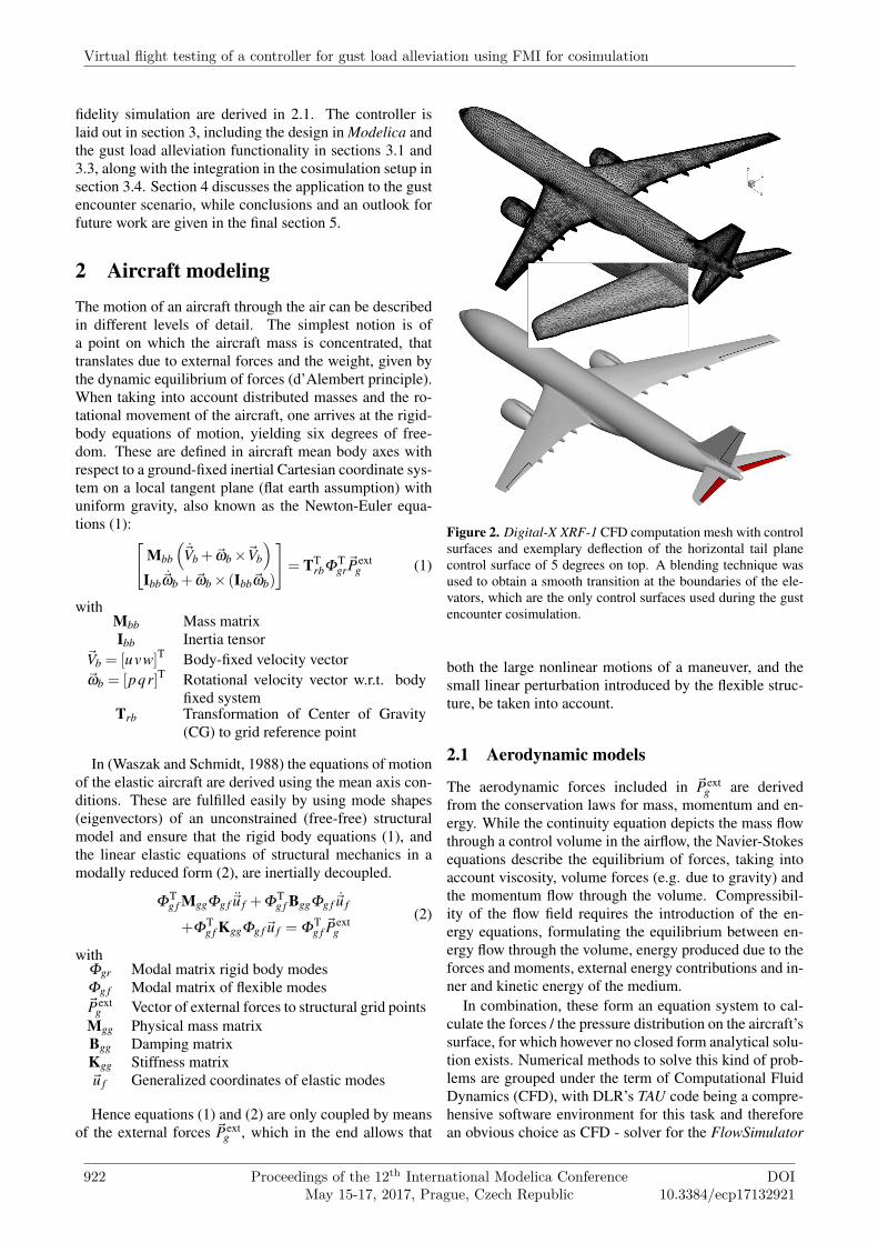
Figure 3. Aircraft aerodynamic model composed of lift sur-faces, for use in the Vortex Lattice Method (VLM) or DoubletLattice Method (DLM), generated by VarLoads. Blue panelsbelong to the aircraft body, purple ones to the control surfaces.

In the beginning of the 20th century, Prandtl found thatfor flows at higher Reynolds numbers Re > 105, the effectof viscosity is approximatively limited to a thin bound-ary layer encompassing the object’s body. Consequently,the flow beyond the boundary layer can be considered asinviscid and importantly, the pressure gradient through itnormal to the surface as zero ( ∂ p

∂ z ≈ 0). In order to ob-tain the pressure distribution on the object’s surface, it istherefore sufficient to calculate it in the inviscid flow justoutside of the boundary layer using the inviscid Navier-Stokes or Euler equations. The assumption of isentropic(no energy contribution/drain) and irrotational flow allowsto define a velocity potential function

~v = grad Φ =[u,v,w

]=[

∂Φ

∂x ,∂Φ

∂y ,∂Φ

∂ z

](3)

which is inserted into the Euler equations. These can

then be linearized around ~v, with the disturbance veloci-ties

[u′,v′,w′

]

~v =

u∞

00

+u′

v′

w′

=

u∞ + ∂ϕ

∂x∂ϕ

∂y∂ϕ

∂ z

(4)

to arrive at the unsteady Prandtl-Glauert equation:

(1−Ma2)∂ 2ϕ

∂x2 +∂ 2ϕ

∂y2 +∂ 2ϕ

∂ z2 −2Ua2

∂ 2ϕ

∂x∂ t− 1

a2∂ 2ϕ

∂ t2 = 0

(5)When neglecting the time-dependent terms, the linear sec-ond order Laplace equation for the Vortex Lattice Method(VLM) (Hedman, 1966) is obtained:

(1−Ma2)∂ 2ϕ

∂x2 +∂ 2ϕ

∂y2 +∂ 2ϕ

∂ z2 = 0. (6)

This method calculates a matrix of Aerodynamic Influ-ence Coefficients (AIC) based on (6) to model lift dis-tributed on an approximation of the aircraft consisting ofseveral lift surfaces as shown in figure 3. The unsteadycounterpart (in the frequency domain) for solving (5) is theDoublet Lattice Method (DLM). External aerodynamicand propulsive forces are added to the inertial forces bymeans of the Force Summation method to calculate resul-tant forces and moments on the aircraft. The loads anal-ysis software VarLoads, which was jointly developed byAirbus and DLR (Hofstee et al., 2003), implements all ofthese modeling and simulation paradigms and was usedto prepare the model with simplified aerodynamics for thecontroller synthesis.

3 Controller design and integration

The Flight Control System (FCS) or short "controller",follows the classical cascaded design layout that is wellstudied in both theory and practice (see e.g. (Brockhauset al., 2011)). This layout is based upon the fact that theaircraft’s equations of motion can be separated into partsthat play a role on different timescales (timescale sepa-ration principle). For example, the body-fixed rotationalrates [p q r]B as fast states are directly linked to the deflec-tion of the control surfaces and resulting moments. On theother hand, states referring to orientation and even moreposition have a slower progression. This allows to dis-sect the flight control system into smaller parts, as shownin figure 4: The inner loop or Stability and Control Aug-mentation (SCA) - block can be designed to stabilize theaircraft and to dampen the dynamic aircraft modes (e.g.phugoid, dutch roll - modes). The autopilot in turn gen-erates a reference orientation for the modified plant ofthe aircraft stabilized by the inner loop. It is designed toachieve a high tracking precision for the desired trajectoryvariables. The additional Gust Load Alleviation (GLA) is

Session 11D: Aerospace

DOI10.3384/ecp17132921


923

arranged at the level of the SCA, since it is assumed herethat the gusts cannot be sensed ahead of the aircraft (e.g.by LIDAR like in Hecker and Hahn (2007)) and necessi-tate fast reactions of the controller / the control surfaces.

FMS AutopilotSCA +GLA

6-DoFrigid body

ϕref,λref,href,

Ψref, . . .

αc,βc,µc,

Vc, . . .

δA,δE ,δR,

δT ,δκ ,δgear

Figure 4. Structure of an electronic flight control system, con-sisting of the FMS and the FCS with autopilot and inner loopSCA. The framed blocks are the considered parts in this work.

As the scenario only considers a frontal vertical gust en-counter, the GLA operates on the longitudinal dynamics,and can symmetrically deflect ailerons and elevators to at-tenuate the gust. Discrimination between inner and outerailerons and elevators as well as distributed spoilers areincorporated in the GLA - layout, but only uniform andsymmetric deflections of likewise δA and δE act as inputs.No actuator dynamics are modeled, due to their absence inthe aircraft model of the cosimulation. Acceleration mea-surements are available at the Center of Gravity (CG) andform the single feedback variable:

nz,m =Lift

Weight=

VK γ

g · cos(Φ)+ cos(γ) (7)

with load factor nz,m, kinematic velocity VK , trajectorypitch angle γ and roll angle Φ. The load factor is fedinto the parameterized GLA filter structure which gener-ates control surface deflection commands, for the elevatorδ

gE with a filter structure containing e.g. a tunable time-

constant. These are then super-positioned to the com-mands of the flight controller:

δi = δci +δ

gi , i ∈ [A,E]. (8)

Hence the autopilot and inner loop also contribute to theload alleviation due to the gust, by acting to hold altitudeand speed.

3.1 Controller model in Modelica

The resulting Flight Control System (FCS) was imple-mented in Modelica using Dymola 2016, and is shown infigure 5. The Modelica Standard - and LinearSystems -libraries provide all of the needed models, with which aflight control library had been established. It consists ofmodules arranged in longitudinal, lateral, inner and outerloop controllers and is also prepared for use in conjunc-tion with DLR’s FlightDynamics library (Looye, 2008).The Dymola simulation tool makes use of the object ori-ented features of Modelica, allowing easy testing and in-terchange of different modules and furthermore offers animplementation of the FMI standard.

In the diagram view depicted in figure 5, the middleleft and the lower center grey rectangular blocks represent

the FCS and the GLA respectively. The FCS consists offour channels for the four individual control effectors ofthe airplane (throttle, elevator, aileron and rudder). Theautopilot modes are set to speed -, altitude - and course- hold, while the commanded sideslip angle βc is zero.The inner loop receives orientation commands from theautopilot and calculates corresponding rates and controlsurface deflections. Each of the channels includes a set ofseveral cascaded linear controllers. To ensure robustnessover the flight envelope, multiple gust - and load - cases,a robust controller synthesis process would normally beappropriate. However, since only one gust encounter caseis considered in this study, a simple tuning of the controllergains has been performed to minimize the effect on thewing root bending moment (see section 3.3).

Figure 5. Modelica model of the longitudinal controller withgust load alleviation.

3.2 Initialization of the FMUEach of the four channel’s inner loops mentioned in thelast section contain either integrator or derivative blockswith internal states that have to be initialized correctly toavoid transient oscillations in the beginning of the simu-lation. Furthermore the cosimulation must be compatiblewith both aircraft models and their respective trim algo-rithms. The given variables of the initialization process arethe reference inputs~ureference and feedback inputs~ufeedbackfrom the aircraft, while the unknowns are the FMU out-puts ~ucontrol (see figure 1). Hence a two-step initializationof the closed-loop simulation setup is performed:

• At first, the aircraft is trimmed separately for steadyhorizontal flight at a given speed and altitude (see ta-ble 1 for a set of characteristic state values), withoutthe controller. This yields values for e.g. α and Θ

and also for elevator deflection δE and throttle δT1.

1The initial values of the lateral effectors δA and δR are zero.



DOI10.3384/ecp17132921

• In the second step, the Functional Mockup Unit(FMU) outputs need to be set to the aircraft controlinput values (~ucontrol) obtained in step 1. Yet dueto FMI design, which prevents variables with out-put causality from the assignment of any value, addi-tional trim parameters have to be defined.

Table 1. Trim values for aircraft model used for controller syn-thesis

Property Unit Value

Mach number - 0.83Altitude ft 35000Reference velocity m/s 246.1Aircraft mass kg 198540Angle of attack ◦ 4.55Gust gradient H m 85.9Gust velocity in z - direction m/s −4.296

−+ kΘ GRC −+ kp

I ki

++

Θc

Θ

q

∆Θ Θ

Φ,V

qc ∆q qc

Figure 6. Inner loop pitch channel, with pitch angle Θ, pitchrate q and GRC as transfer function containing the correction forturning flight (increase in pitch due to rotated lift vector).

This second step is further explained using the example ofthe inner loop pitch channel shown in figure 6: With givenδE,trim and Θtrim, the single degree of freedom is the initialstate value of the integrator. The trim pitch angle is addedto the autopilot command

Θc = ∆ΘAP +Θtrim, (9)

where ∆ΘAP is zero here due to initial h = hc. Likewisethe elevator command consists of

δE = qc +δE,trim +δE,GLA. (10)

With the constraint of steady state integrator initialization(xint = 0), and similar provisions for the velocity channel,the initial equation of the controller model has to be speci-fied as shown in listing 1. By calling the initialize()- method of the FMU, the controller can then match thepreceding aircraft trim.

Listing 1. Initial equation of the controller model

i n i t i a l equat ionc o n t r o l l e r L o n g i t u d i n a l . y [ 1 ] = t r im_de_T ;c o n t r o l l e r L o n g i t u d i n a l . y [ 2 ] = t r im_de_E ;

3.3 Synthesis of the GLA controller

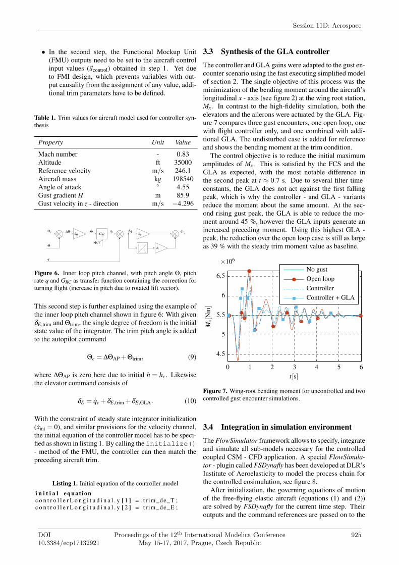
The controller and GLA gains were adapted to the gust en-counter scenario using the fast executing simplified modelof section 2. The single objective of this process was theminimization of the bending moment around the aircraft’slongitudinal x - axis (see figure 2) at the wing root station,Mx. In contrast to the high-fidelity simulation, both theelevators and the ailerons were actuated by the GLA. Fig-ure 7 compares three gust encounters, one open loop, onewith flight controller only, and one combined with addi-tional GLA. The undisturbed case is added for referenceand shows the bending moment at the trim condition.

The control objective is to reduce the initial maximumamplitudes of Mx. This is satisfied by the FCS and theGLA as expected, with the most notable difference inthe second peak at t ≈ 0.7 s. Due to several filter time-constants, the GLA does not act against the first fallingpeak, which is why the controller - and GLA - variantsreduce the moment about the same amount. At the sec-ond rising gust peak, the GLA is able to reduce the mo-ment around 45 %, however the GLA inputs generate anincreased preceding moment. Using this highest GLA -peak, the reduction over the open loop case is still as largeas 39 % with the steady trim moment value as baseline.

Controller + GLA

Controller

Open loop

No gust

Mx[N

m]

t[s]

0 1 2 3 4 5 6

×106

4.5

5

5.5

6

6.5

Figure 7. Wing-root bending moment for uncontrolled and twocontrolled gust encounter simulations.

3.4 Integration in simulation environment

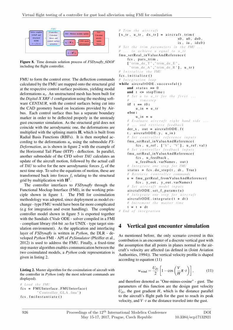
The FlowSimulator framework allows to specify, integrateand simulate all sub-models necessary for the controlledcoupled CSM - CFD application. A special FlowSimula-tor - plugin called FSDynafly has been developed at DLR’sInstitute of Aeroelasticity to model the process chain forthe controlled cosimulation, see figure 8.

After initialization, the governing equations of motionof the free-flying elastic aircraft (equations (1) and (2))are solved by FSDynafly for the current time step. Theiroutputs and the command references are passed on to the


DOI10.3384/ecp17132921


925

Solve coupled6-DoF andstructural

EOMx = f (x,x)

Controller:Calculatethrust and

control surfaceactuation

FMU

TAU: Motion module update

ua = H usCFD meshdeformation

fs = HT fa

TAU:Calculateaerody-namicforces

Figure 8. Time domain solution process of FSDynafly_6DOFincluding the flight controller.

FMU to form the control error. The deflection commandscalculated by the FMU are mapped onto the structural gridat the respective control surface positions, yielding modaldeformations us. An unstructured mesh has been built forthe Digital-X XRF-1 configuration using the meshing soft-ware CENTAUR, with the control surfaces being cut intothe CAD geometry based on locations provided by Air-bus. Each control surface thus has a separate boundarymarker in order to be deflected properly in the unsteadygust encounter simulation. As the structural grid does notcoincide with the aerodynamic one, the deformations aremultiplied with the splining matrix H, which is built fromRadial Basis Functions (RBFs). It is then morphed ac-cording to the deformations ua using the submodule FS-Deformation, as is shown in figure 2 with the example ofthe Horizontal Tail Plane (HTP) - deflection. In parallel,another submodule of the CFD solver TAU calculates anupdate of the aircraft motion, followed by the actual callof TAU to solve for the new aerodynamic forces fa of thenext time step. To solve the equations of motion, these aretransformed back into forces fs relating to the structuralgrid by multiplication with HT.

The controller interfaces to FSDynafly through theFunctional Mockup Interface (FMI), in the working prin-ciple shown in figure 1. The FMI for cosimulationmethodology was adopted, since deployment as model ex-change - type FMU would have been far more complicated(e.g for integration and event handling). The completecontroller model shown in figure 5 is exported togetherwith the Sundials CVode ODE - solver compiled in a FMI- compliant library (64-bit .so for UNIX - type target sim-ulation environment). As the application and interfacinglayer of FSDynafly is written in Python, the DLR - de-veloped Python FMI - API of PySimulator (Pfeiffer et al.,2012) is used to address the FMU. Finally, a fixed-timestep master algorithm enables communication between thetwo cosimulated models, a Python code representation isgiven in listing 2.

Listing 2. Master algorithm for the cosimulation of aircraft withthe controller in Python (only the most relevant commands aredisplayed).

# Load t h e FMUf c s = FMUInte r face . FMUInte r face (

" Cont ro l l e r_GLA . fmu " )f c s . f m i I n s t a n t i a t e ( )

# Trim t h e a i r c r a f t[ x _ t r , u _ t r , d x _ t r ] = a i r c r a f t . t r i m (

x0 , u0 , dx0 ,ix , iu , i dx0 )

# S e t t h e t r i m p a r a m e t e r s i n t h e FMU . . .# . . . t o a c h i e v e u e q u a l t o u _ t rf m u _ s e t R e a l _ i n V a l u e A n d R e f e r e n c e (

f c s , p a r s _ t r i m ,[ " t r im_de_T " , " t r im_de_E " ,

" t r im_de_A " , " t r im_de_R " ] , u _ t r )# I n i t i a l i z e t h e FMUf c s . i n i t i a l i z e ( )# I n t e g r a t i o n loopwhi le a i r c r a f t O D E . s u c c e s s f u l ( )

and s t a t u s == 0and t <= s topTime :# S e t u t o u _ t r f o r t h e f i r s t . . .# . . . t i m e s t e pi f t == t 0 :

u_ in = u _ t re l s e :

u_ in = u# E v a l u a t e a i r c r a f t r i g h t hand s i d e . . .# . . . and r e t r i e v e f e e d b a c kder_x , o u t = a i r c r a f t O D E . f (t , a i r c r a f t O D E . y , u_ in )# S e t c o n t r o l l e r r e f e r e n c e i n p u t sf m u _ s e t R e a l _ i n V a l u e A n d R e f e r e n c e (

f c s , u _ r e f , [ " h " , "V" ] , u _ r e f . v a l )# S e t c o n t r o l l e r f e e d b a c k i n p u t sf m u _ s e t R e a l _ i n V a l u e A n d R e f e r e n c e (

f c s , u_feedback ,u _ f e e d b a c k . varNames , o u t )

# I n t e g r a t e one s t e p f o r FMUs t a t u s = f c s . d o _ s t e p ( t , d t , True )# R e t r i e v e c o n t r o l l e r commandsu = fmu_ge tRea l_ f romValueAndRefe rence (

f c s , y_out , y_ou t . varNames )# S e t a i r c r a f t model i n p u t sa i r c r a f t O D E . s e t _ f _ p a r a m s ( u )# I n t e g r a t e one s t e p f o r a i r c r a f ta i r c r a f t O D E . i n t e g r a t e ( t + d t )# I n c r e m e n t t h e m as t e r t i m et = t + d t

# End o f i n t e g r a t i o n

4 Vertical gust encounter simulationAs mentioned before, the only scenario covered in thiscontribution is an encounter of a discrete vertical gust withthe assumption that all points in planes normal to the air-craft’s velocity are affected (as defined in (Joint AviationAuthorities, 1994)). The vertical velocity profile is shapedaccording to equation (11)

wwind =Uds

2

[1− cos

(VH

π · t)]

, (11)

and therefore denoted as "One-minus-cosine" - gust. Theparameters of this function are the design gust velocityUds, the gust gradient H, which is the distance parallelto the aircraft’s flight path for the gust to reach its peakvelocity, and V · t as the distance traveled into the gust.



DOI10.3384/ecp17132921

Ctrl

Cosim

ww

ind[m

/s]

t [s]

0 0.2 0.4 0.6 0.8 1

0

1

2

3

4

5

Figure 9. One minus cosine gust definitions used for the com-plete cosimulation and for the controller synthesis.

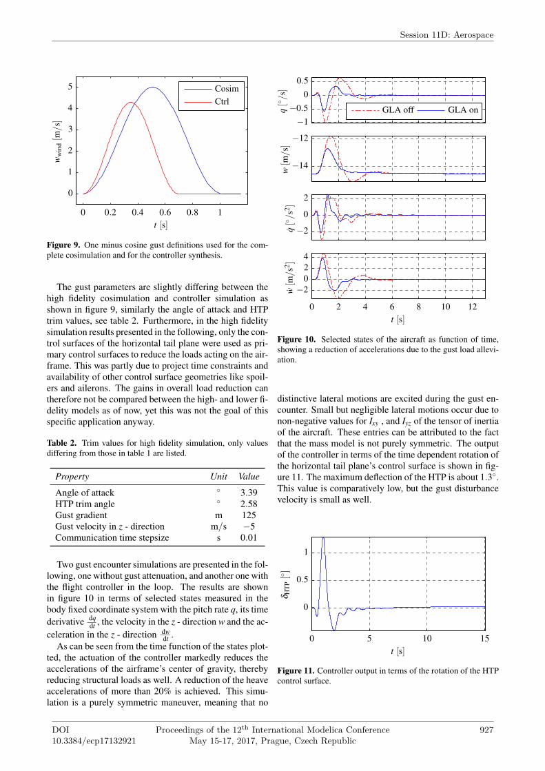
The gust parameters are slightly differing between thehigh fidelity cosimulation and controller simulation asshown in figure 9, similarly the angle of attack and HTPtrim values, see table 2. Furthermore, in the high fidelitysimulation results presented in the following, only the con-trol surfaces of the horizontal tail plane were used as pri-mary control surfaces to reduce the loads acting on the air-frame. This was partly due to project time constraints andavailability of other control surface geometries like spoil-ers and ailerons. The gains in overall load reduction cantherefore not be compared between the high- and lower fi-delity models as of now, yet this was not the goal of thisspecific application anyway.

Table 2. Trim values for high fidelity simulation, only valuesdiffering from those in table 1 are listed.

Property Unit Value

Angle of attack ◦ 3.39HTP trim angle ◦ 2.58Gust gradient m 125Gust velocity in z - direction m/s −5Communication time stepsize s 0.01

Two gust encounter simulations are presented in the fol-lowing, one without gust attenuation, and another one withthe flight controller in the loop. The results are shownin figure 10 in terms of selected states measured in thebody fixed coordinate system with the pitch rate q, its timederivative dq

dt , the velocity in the z - direction w and the ac-celeration in the z - direction dw

dt .As can be seen from the time function of the states plot-

ted, the actuation of the controller markedly reduces theaccelerations of the airframe’s center of gravity, therebyreducing structural loads as well. A reduction of the heaveaccelerations of more than 20% is achieved. This simu-lation is a purely symmetric maneuver, meaning that no

t [s]

w[m

/s2]

q[◦/s

2]

w[m

/s]

GLA onGLA offq[◦/s]

0 2 4 6 8 10 12

−2

0

2

4

−2

0

2

−14

−12

−1

−0.5

0

0.5

Figure 10. Selected states of the aircraft as function of time,showing a reduction of accelerations due to the gust load allevi-ation.

distinctive lateral motions are excited during the gust en-counter. Small but negligible lateral motions occur due tonon-negative values for Ixy , and Iyz of the tensor of inertiaof the aircraft. These entries can be attributed to the factthat the mass model is not purely symmetric. The outputof the controller in terms of the time dependent rotation ofthe horizontal tail plane’s control surface is shown in fig-ure 11. The maximum deflection of the HTP is about 1.3◦.This value is comparatively low, but the gust disturbancevelocity is small as well.

δH

TP[◦]

t [s]

0 5 10 15

0

0.5

1

Figure 11. Controller output in terms of the rotation of the HTPcontrol surface.


DOI10.3384/ecp17132921


927

5 Conclusion and outlook

In this contribution, a new methodology for loads analysisand virtual flight testing of flight controllers is presented.Usually disconnected simulation steps are combined intoa single process chain, including elastic structural aircraftmodeling, full Navier-Stokes aerodynamics and a flightcontrol system with gust load alleviation.

A flight controller with outer and inner loop, as well asgust load alleviation system was set up in Modelica usingDymola. It was tuned for a gust encounter scenario using aVortex Lattice Method (VLM) based aerodynamic model,allowing the required large number of simulations duringcontroller synthesis. A final reduction of up to 45% in thewing root bending moment was found there.

A setup for the cosimulation was developed in Python,including a fixed-step master algorithm connecting thesimulation framework FSDynafly with the controller. Byemploying the FMI standard to interface the controller,dedicated API development for the dissimilar aircraftmodels could be omitted. Furthermore the functionalitiesof FMI for cosimulation allowed an easy setup and effi-cient operation of the controlled high fidelity simulation.Reductions in the vertical and the pitch accelerations of upto 20 % were achieved, also consequentially leading to areduction in the structural loads.

After successfully completing this first proof of con-cept, future work will be directed towards functionalityin larger simulation studies with multi-parameter or evenmulti-model test cases and different scenarios (e.g. ma-neuver loads, flight performance analysis). Ensuring therobustness of the controller for the entire flight envelopewill be an important prerequisite for these applications,and could be achieved by employing methods from robustcontrol design (e.g. H∞ or robust LPV control).

An immediate next step will be the addition of new con-trol surfaces (ailerons and possibly spoilers) to the CFDmesh, since currently the only means of controlling theaircraft and the loads is the horizontal tail plane. Based onthe results of the simplified aerodynamics simulation, it isexpected that loads on the main wing can be further re-duced by this approach. As well, it should be worthwhileto incorporate additional design criteria in the controllersynthesis process. By treating it as a multi-objective opti-mization problem, the investigation of trade offs betweene.g. load reduction, passenger comfort and flying qualitiesis made possible.

6 Acknowledgments

This work was prepared during the course of DLR projectDigital-X. The authors would like to express their thanksto the following colleagues for their support and input:Martin Leitner, Hans-Dieter Joos, Andreas Pfeiffer andThiemo Kier.

ReferencesRudolf Brockhaus, Wolfgang Alles, and Robert Luckner.

Flugregelung. Springer, 2011. ISBN 9783642014437.URL http://books.google.de/books?id=2IKXH3skXBwC.

Simon Hecker and Klaus-Uwe Hahn. Advanced gust load alle-viation system for large flexible aircraft. In Proceeding 1stCEAS Konferenz, 2007.

Sven G Hedman. Vortex lattice method for calculation of quasisteady state loadings on thin elastic wings in subsonic flow.Technical report, DTIC Document, 1966.

Jeroen Hofstee, Thiemo Kier, Chiara Cerulli, and GertjanLooye. A variable, fully flexible dynamic response tool forspecial investigations (VarLoads). In 2003 CEAS/AIAA/NVvLInternational Forum on Aeroelasticity and Structural Dynam-ics, 2003.

Joint Aviation Authorities. Joint aviation requirements. JAR-25. Large aeroplanes. Civil Aviation Authority Printing &Publication Services, Greville House, 37, 1994.

Norbert Kroll, Mohammad Abu-Zurayk, Diliana Dimitrov,T Franz, Tanja Führer, Thomas Gerhold, Stefan Görtz, RalfHeinrich, Caslav Ilic, Jonas Jepsen, et al. DLR projectDigital-X: towards virtual aircraft design and flight testingbased on high-fidelity methods. CEAS Aeronautical Journal,7(1):3–27, 2016.

Gertjan Looye. The new DLR flight dynamics library. In Pro-ceedings of the 6th International Modelica Conference, vol-ume 1, pages 193–202, 2008.

Michael Meinel and Gunnar O Einarsson. The FlowSimulatorframework for massively parallel CFD applications. PARA2010, 2010.

Functional Mock-up Interface for Model Exchange and Co-Simulation, Version 2.0. Modelica Association, July 2014.

Andreas Pfeiffer, Matthias Hellerer, Stefan Hartweg, Martin Ot-ter, and Matthias Reiner. PySimulator-A Simulation andAnalysis Environment in Python with Plugin Infrastructure.In Proceedings of the 9th International MODELICA Confer-ence; September 3-5; 2012; Munich; Germany, pages 523–536. Linköping University Electronic Press, 2012. 76.

Dieter Schwamborn, Thomas Gerhold, and Ralf Heinrich. TheDLR TAU-Code: recent applications in research and indus-try. In ECCOMAS CFD 2006: Proceedings of the EuropeanConference on Computational Fluid Dynamics, Egmond aanZee, The Netherlands, September 5-8, 2006. Delft Univer-sity of Technology; European Community on ComputationalMethods in Applied Sciences (ECCOMAS), 2006.

Martin R Waszak and David K Schmidt. Flight dynamics ofaeroelastic vehicles. Journal of Aircraft, 25(6):563–571,1988.



DOI10.3384/ecp17132921

Virtual ight testing of a controller for gust load ... · Virtual ight testing of a controller for...

Documents

Transcript of Virtual ight testing of a controller for gust load ... · Virtual ight testing of a controller for...