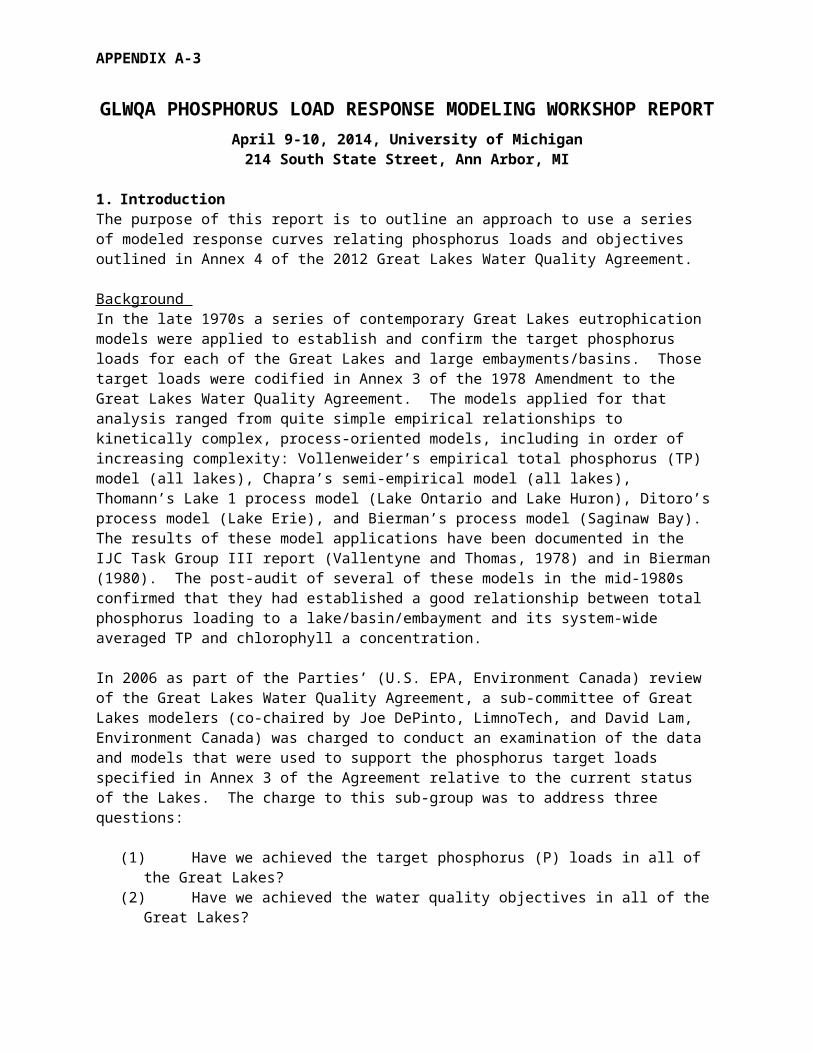
APPENDIX A-3

GLWQA PHOSPHORUS LOAD RESPONSE MODELING WORKSHOP REPORT April 9-10, 2014, University of Michigan214 South State Street, Ann Arbor, MI

1. IntroductionThe purpose of this report is to outline an approach to use a series of modeled response curves relating phosphorus loads and objectives outlined in Annex 4 of the 2012 Great Lakes Water Quality Agreement.

Background In the late 1970s a series of contemporary Great Lakes eutrophication models were applied to establish and confirm the target phosphorus loads for each of the Great Lakes and large embayments/basins. Those target loads were codified in Annex 3 of the 1978 Amendment to the Great Lakes Water Quality Agreement. The models applied for that analysis ranged from quite simple empirical relationships to kinetically complex, process-oriented models, including in order of increasing complexity: Vollenweider’s empirical total phosphorus (TP) model (all lakes), Chapra’s semi-empirical model (all lakes), Thomann’s Lake 1 process model (Lake Ontario and Lake Huron), Ditoro’s process model (Lake Erie), and Bierman’s process model (Saginaw Bay). The results of these model applications have been documented in the IJC Task Group III report (Vallentyne and Thomas, 1978) and in Bierman (1980). The post-audit of several of these models in the mid-1980s confirmed that they had established a good relationship between total phosphorus loading to a lake/basin/embayment and its system-wide averaged TP and chlorophyll a concentration.

In 2006 as part of the Parties’ (U.S. EPA, Environment Canada) review of the Great Lakes Water Quality Agreement, a sub-committee of Great Lakes modelers (co-chaired by Joe DePinto, LimnoTech, and David Lam, Environment Canada) was charged to conduct an examination of the data and models that were used to support the phosphorus target loads specified in Annex 3 of the Agreement relative to the current status of the Lakes. The charge to this sub-group was to address three questions:

(1) Have we achieved the target phosphorus (P) loads in all of the Great Lakes?(2) Have we achieved the water quality objectives in all of the Great Lakes?(3) Can we define the quantitative relationships between P loads and lake conditions with existing

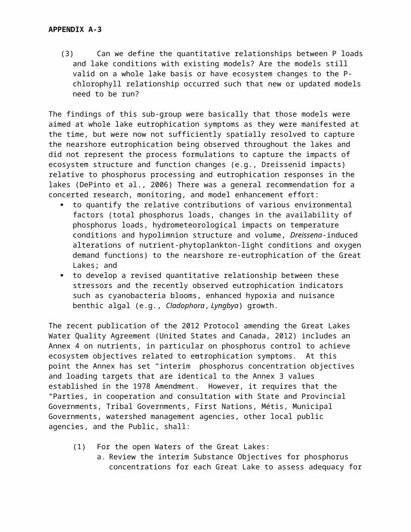
models? Are the models still valid on a whole lake basis or have ecosystem changes to the P- chlorophyll relationship occurred such that new or updated models need to be run?

The findings of this sub-group were basically that those models were aimed at whole lake eutrophication symptoms as they were manifested at the time, but were now not sufficiently spatially resolved to capture the nearshore eutrophication being observed throughout the lakes and did not represent the process formulations to capture the impacts of ecosystem structure and function changes (e.g., Dreissenid impacts) relative to phosphorus processing and eutrophication responses in the lakes (DePinto et al., 2006) There was a general recommendation for a concerted research, monitoring, and model enhancement effort:

to quantify the relative contributions of various environmental factors (total phosphorus loads, changes in the availability of phosphorus loads, hydrometeorological impacts on temperature conditions and hypolimnion structure and volume, Dreissena-induced alterations of nutrient-phytoplankton-light conditions and oxygen demand functions) to the nearshore re-eutrophication of the Great Lakes; and

APPENDIX A-3

to develop a revised quantitative relationship between these stressors and the recently observed eutrophication indicators such as cyanobacteria blooms, enhanced hypoxia and nuisance benthic algal (e.g., Cladophora, Lyngbya) growth.

The recent publication of the 2012 Protocol amending the Great Lakes Water Quality Agreement (United States and Canada, 2012) includes an Annex 4 on nutrients, in particular on phosphorus control to achieve ecosystem objectives related to eutrophication symptoms. At this point the Annex has set “interim” phosphorus concentration objectives and loading targets that are identical to the Annex 3 values established in the 1978 Amendment. However, it requires that the “Parties, in cooperation and consultation with State and Provincial Governments, Tribal Governments, First Nations, Métis, Municipal Governments, watershed management agencies, other local public agencies, and the Public, shall:

(1) For the open Waters of the Great Lakes: a. Review the interim Substance Objectives for phosphorus concentrations for each

Great Lake to assess adequacy for the purpose of meeting Lake Ecosystem Objectives, and revise as necessary;

b. Review and update the phosphorus loading targets for each Great Lake; and c. Determine appropriate phosphorus loading allocations, apportioned by country,

necessary to achieve Substance Objectives for phosphorus concentrations for each Great Lake;

(2) For the nearshore Waters of the Great Lakes:a. Develop Substance Objectives for phosphorus concentrations for nearshore waters,

including embayments and tributary discharge for each Great Lake; andb. Establish load reduction targets for priority watersheds that have a significant

localized impact on the Waters of the Great Lakes.

The Annex also calls for research and other programs aimed at setting and achieving the revised nutrient objectives. It also calls for the Parties to take into account the bioavailability of various forms of phosphorus, related productivity, seasonality, fisheries productivity requirements, climate change, invasive species, and other factors, such as downstream impacts, as necessary, when establishing the updated phosphorus concentration objectives and loading targets. Finally, it calls for the Lake Erie objectives and loading target revisions to be completed within three years of the 2012 Agreement entry into force.

To assist the Parties in developing and applying an approach for accomplishing these mandates, we developed the approach outlined in this paper to evaluate the interim phosphorus objectives and load targets for Lake Erie and to propose an approach for updating those targets in light of the new research and monitoring and modeling in the lake. The plan that is developed for Lake Erie can serve as a template for the other Great Lakes in meeting the 2012 Great Lakes Water Quality Agreement Protocol Annex 4 mandates.

Approach and Scope On April 9-10, 2014, LimnoTech and University of Michigan’s Graham Sustainability Institute convened a meeting of Lake Erie modelers, agency personnel, and others to assess the capabilities of existing models to develop response curves between nutrient loads and the objectives being identified by the Annex 4 group. This group’s goal was to develop a plan for conducting an ensemble modeling effort, leading to recommendations to the Annex 4 Objectives Task Team for revised Lake Erie objectives and

APPENDIX A-3

associated target P loads by the end of September 2014. A meeting agenda and list of participants are included in Appendix A-1.

2. Model Evaluation CriteriaDuring the meeting, we used the following criteria to assess the ability of each modeling effort to address the goals. While some level of assessment was done during the meeting, final assessments and decisions on appropriate use will be completed as part of the final product.

Ability to develop load-response curves and/or provide other output important for quantitative understanding of the questions/requirements posed in Annex 4: A key function of the models to be used in this effort is to establish relationships between phosphorus loads and the metric defined by the Annex 4 subgroup for each objective. As such, models will be evaluated as to their ability to establish load-response curves as the highest priority. Other models were also evaluated as to their utility to provide additional information to help understand dynamics, justify relationships, or otherwise inform the response curves or targets.

Applicability to objectives/metrics to be provided by the Annex 4 subgroup: The models will be evaluated as to their ability to address the specific spatial, temporal, and kinetic resolution characteristics of the objectives and metrics outlines by the Annex 4 subgroup. While models that address other objectives and metrics can be additionally informative, the highest priorities are those that can address them directly.

Extent/quality of calibration and confirmation: Calibration - Given the expected range in model type and complexity, there will likely be a range of skill assessments to be used. Models will be evaluated as to their ability to reproduce state-variables that match the objective metrics, as well as internal process dynamics. Post-calibration testing – Models will also be measured against their ability to replicate conditions not represented in the calibration data set.

Extent of model documentation (peer review or otherwise): Models will be evaluated based on the extent of their documentation. Full descriptions of model kinetics, inputs, calibration, confirmation, and applications are expected. This can be done through copies of peer reviewed journal articles, government reports, or other documentation, but it must be in writing.

Level of uncertainty analysis available: Models will be evaluated as to the extent they are able to quantify aspects of model uncertainty, including uncertainties associated with observation measurement error, model structure, parameterization, and aggregation, as well as uncertainty associated with characterizing natural variability.

3. Current modeling efforts to address response indicators As mentioned above an initial recommendation must be put forth by the Annex 4 Objectives Task Group by the Fall of 2014. This deadline did not afford the time to go through a formal model comparison, vetting and evaluation process; hence this workshop was held to identify the eutrophication response indicators of concern and the models currently available to address those indicators. It also provided for an informal vetting of these models.

The first task related to the short-term goal is to identify the Eutrophication Response Indicators (ERIs) of concern for Lake Erie. We have identified the following four ERIs, along with metrics used to model

APPENDIX A-3

and track them. This involves defining the metric in terms of how it is measured and what spatial and temporal scale will be used for that metric measurement.

(1) Overall phytoplankton biomass as represented by chlorophyll a Basin-specific, summer (June-August) average chlorophyll concentration

This is a traditional indicator of lake trophic status (i.e., oligotrophic, mesotrophic, eutrophic).

(2) Cyanobacteria blooms (including Microcystis sp.) in the Western Basin Maximum basin-wide cyanobacteria biomass (mass dry weight) Summer total basin-wide cyanobacteria biomass (mass dry weight integrated over

summer bloom period)

The first metric gives an indication of the worst condition relative to HABs in the Western Basin, while the second factors in the cumulative effects of multiple drivers (loads, hydrology, wind, temperature, etc.) in producing a season-long cumulative production of HABs. The length of the “summer bloom period” referred to in this metric can vary from one scenario to another.

(3) Hypoxia in hypolimnion of the Central Basin Number of hypoxic days Average areal extent during summer Average hypolimnion DO concentration during stratification

All three of these metrics are quantitatively correlated based on Central Basin monitoring and analysis, but they are different manifestations of the problem that each has a bearing on the assessment of the impact on the ecosystem (especially fish communities) and on the relative impact of physical conditions and nutrient-algal growth conditions on the indicator.

(4) Cladophora in the nearshore areas of the Eastern Basin

While beach fouling by sloughed Cladophora is likely the most important metric, there is neither an acceptable monitoring program to measure and report progress, nor a scientifically credible model to relate it to nutrient loads and conditions. There are models that can relate Cladophora growth to ambient DRP concentration and models that can estimate near shore DRP as a function of loads and biophysical dynamics. Linking these models could allow us to then relate loads to Cladophora growth, but the accumulation of errors across models minimizes the utility as a predictor. Instead, what would be useful is to use these models to explore the relative impacts of loads recommended for other objectives eutrophication response indicators on Cladophora growth potential.

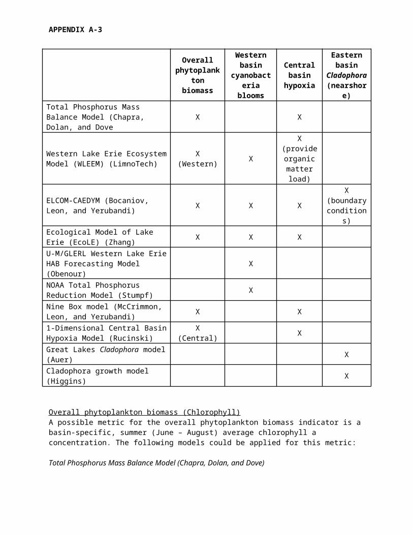
The models capable of addressing each of these indicators have been identified and described briefly below and summarized in Table A3-1.

APPENDIX A-3

Table A3-1: Models considered for ensemble modeling effort, organized according to capability to address selected ecosystem response indicators.

Model

Response Indicators

Overall phytoplankton

biomass

Western basin

cyanobacteria blooms

Central basin

hypoxia

Eastern basin Cladophora (nearshore)

Total Phosphorus Mass Balance Model (Chapra, Dolan, and Dove X X

Western Lake Erie Ecosystem Model (WLEEM) (LimnoTech) X (Western) X

X (provide organic

matter load)ELCOM-CAEDYM (Bocaniov, Leon, and Yerubandi) X X X X (boundary

conditions)Ecological Model of Lake Erie (EcoLE) (Zhang) X X X

U-M/GLERL Western Lake Erie HAB Forecasting Model (Obenour) X

NOAA Total Phosphorus Reduction Model (Stumpf) X

Nine Box model (McCrimmon, Leon, and Yerubandi) X X

1-Dimensional Central Basin Hypoxia Model (Rucinski) X (Central) X

Great Lakes Cladophora model (Auer) XCladophora growth model (Higgins) X

Overall phytoplankton biomass (Chlorophyll)A possible metric for the overall phytoplankton biomass indicator is a basin-specific, summer (June – August) average chlorophyll a concentration. The following models could be applied for this metric:

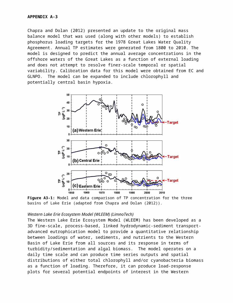
Total Phosphorus Mass Balance Model (Chapra, Dolan, and Dove)Chapra and Dolan (2012) presented an update to the original mass balance model that was used (along with other models) to establish phosphorus loading targets for the 1978 Great Lakes Water Quality Agreement. Annual TP estimates were generated from 1800 to 2010. The model is designed to predict the annual average concentrations in the offshore waters of the Great Lakes as a function of external loading and does not attempt to resolve finer-scale temporal or spatial variability. Calibration data for this model were obtained from EC and GLNPO. The model can be expanded to include chlorophyll and potentially central basin hypoxia.

APPENDIX A-3

Figure A3-1: Model and data comparison of TP concentration for the three basins of Lake Erie (adapted from Chapra and Dolan (2012)).

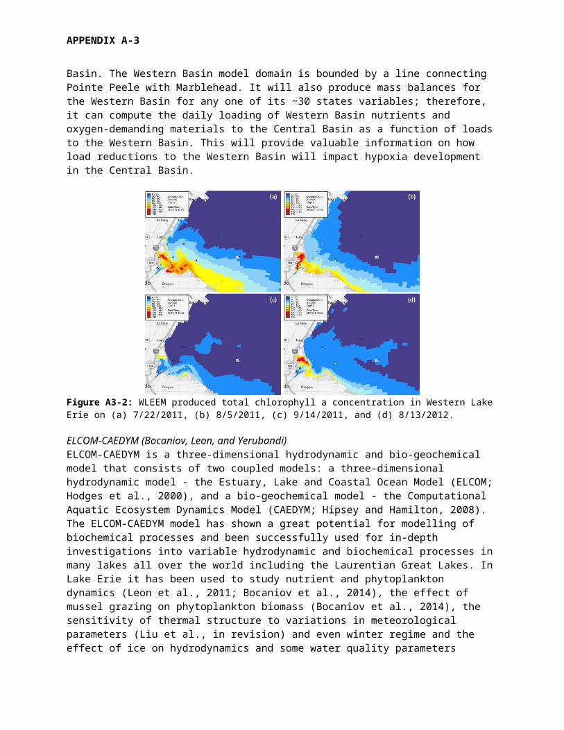
Western Lake Erie Ecosystem Model (WLEEM) (LimnoTech)The Western Lake Erie Ecosystem Model (WLEEM) has been developed as a 3D fine-scale, process-based, linked hydrodynamic-sediment transport-advanced eutrophication model to provide a quantitative relationship between loadings of water, sediments, and nutrients to the Western Basin of Lake Erie from all sources and its response in terms of turbidity/sedimentation and algal biomass. The model operates on a daily time scale and can produce time series outputs and spatial distributions of either total chlorophyll and/or cyanobacteria biomass as a function of loading. Therefore, it can produce load-response plots for several potential endpoints of interest in the Western Basin. The Western Basin model domain is bounded by a line connecting Pointe Peele with Marblehead. It will also produce mass balances for the Western Basin for any one of its ~30 states variables; therefore, it can compute the daily loading of Western Basin nutrients and oxygen-demanding materials to the Central Basin as a function of loads to the Western Basin. This will provide valuable information on how load reductions to the Western Basin will impact hypoxia development in the Central Basin.

APPENDIX A-3

Figure A3-2: WLEEM produced total chlorophyll a concentration in Western Lake Erie on (a) 7/22/2011, (b) 8/5/2011, (c) 9/14/2011, and (d) 8/13/2012.

ELCOM-CAEDYM (Bocaniov, Leon, and Yerubandi)ELCOM-CAEDYM is a three-dimensional hydrodynamic and bio-geochemical model that consists of two coupled models: a three-dimensional hydrodynamic model - the Estuary, Lake and Coastal Ocean Model (ELCOM; Hodges et al., 2000), and a bio-geochemical model - the Computational Aquatic Ecosystem Dynamics Model (CAEDYM; Hipsey and Hamilton, 2008). The ELCOM-CAEDYM model has shown a great potential for modelling of biochemical processes and been successfully used for in-depth investigations into variable hydrodynamic and biochemical processes in many lakes all over the world including the Laurentian Great Lakes. In Lake Erie it has been used to study nutrient and phytoplankton dynamics (Leon et al., 2011; Bocaniov et al., 2014), the effect of mussel grazing on phytoplankton biomass (Bocaniov et al., 2014), the sensitivity of thermal structure to variations in meteorological parameters (Liu et al., in revision) and even winter regime and the effect of ice on hydrodynamics and some water quality parameters (Oveisy et al., in revision). The application of ELCOM-CAEDYM model to study the oxygen dynamics and understand the central basin hypoxia is a subject of the ongoing work.

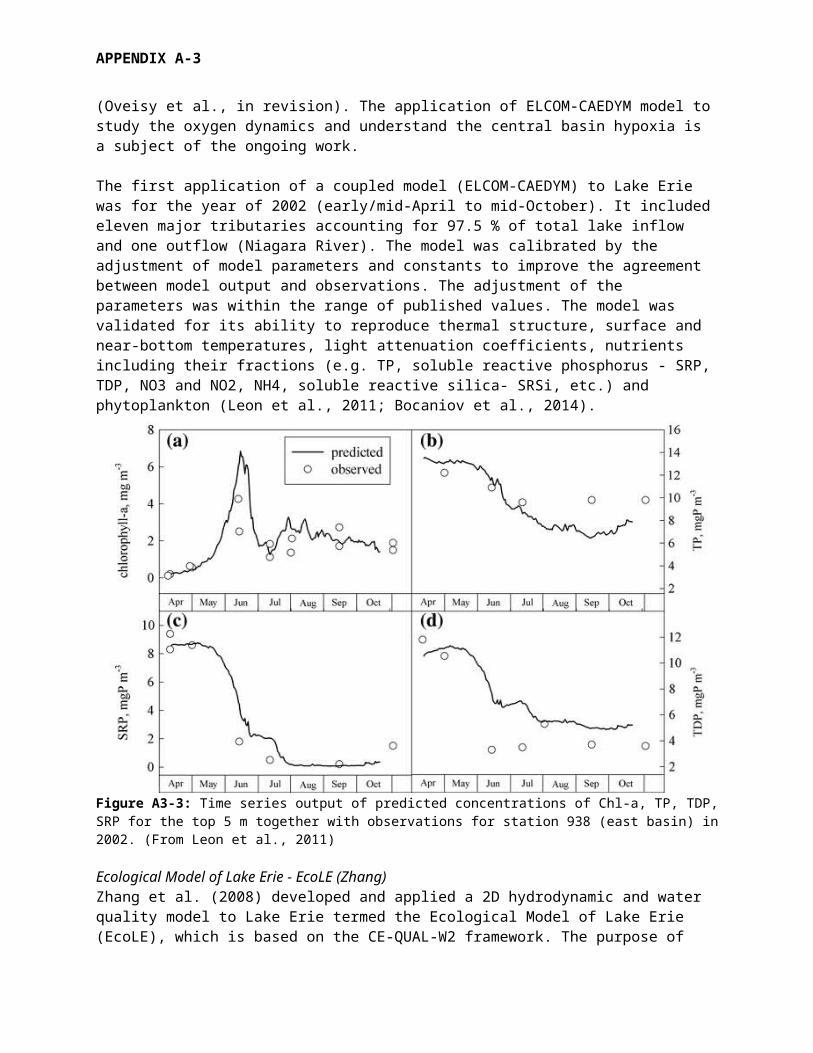
The first application of a coupled model (ELCOM-CAEDYM) to Lake Erie was for the year of 2002 (early/mid-April to mid-October). It included eleven major tributaries accounting for 97.5 % of total lake inflow and one outflow (Niagara River). The model was calibrated by the adjustment of model parameters and constants to improve the agreement between model output and observations. The adjustment of the parameters was within the range of published values. The model was validated for its ability to reproduce thermal structure, surface and near-bottom temperatures, light attenuation coefficients, nutrients including their fractions (e.g. TP, soluble reactive phosphorus - SRP, TDP, NO3 and NO2, NH4, soluble reactive silica- SRSi, etc.) and phytoplankton (Leon et al., 2011; Bocaniov et al., 2014).

APPENDIX A-3

Figure A3-3: Time series output of predicted concentrations of Chl-a, TP, TDP, SRP for the top 5 m together with observations for station 938 (east basin) in 2002. (From Leon et al., 2011)

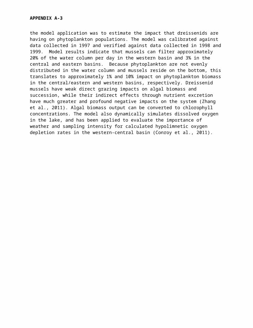
Ecological Model of Lake Erie - EcoLE (Zhang)Zhang et al. (2008) developed and applied a 2D hydrodynamic and water quality model to Lake Erie termed the Ecological Model of Lake Erie (EcoLE), which is based on the CE-QUAL-W2 framework. The purpose of the model application was to estimate the impact that dreissenids are having on phytoplankton populations. The model was calibrated against data collected in 1997 and verified against data collected in 1998 and 1999. Model results indicate that mussels can filter approximately 20% of the water column per day in the western basin and 3% in the central and eastern basins. Because phytoplankton are not evenly distributed in the water column and mussels reside on the bottom, this translates to approximately 1% and 10% impact on phytoplankton biomass in the central/eastern and western basins, respectively. Dreissenid mussels have weak direct grazing impacts on algal biomass and succession, while their indirect effects through nutrient excretion have much greater and profound negative impacts on the system (Zhang et al., 2011). Algal biomass output can be converted to chlorophyll concentrations. The model also dynamically simulates dissolved oxygen in the lake, and has been applied to evaluate the importance of weather and sampling intensity for calculated hypolimnetic oxygen depletion rates in the western-central basin (Conroy et al., 2011).

APPENDIX A-3

Figure A3-4: EcoLE model verification of 1998 for non-diatom edible algae, diatoms, copepods, cladocerans, total dissolved phosphorus (TP-F), and ammonia (NH4).

Western Basin cyanobacterial bloomsPossible metrics for the Western Basin cyanobacterial blooms indicator could include: maximum basin-wide cyanobacteria biomass or summer average cyanobacteria biomass in the basin. This metric therefore requires a model that is specific for the cyanobacteria functional group and either provides a time-variable simulation of that functional group or an empirical relationship for the metric in question. The Obenour and Stumpf models produce empirical relationships between spring loading (approximately March-June) from the Maumee River and the maximum cyanobacteria biomass. The ELCOM-CAEDYM, WLEEM and EcoLE models all compute the cyanobacteria biomass on a time-variable basis and at a spatial resolution such that they can compute both maximum and summer average cyanobacteria biomass.

APPENDIX A-3

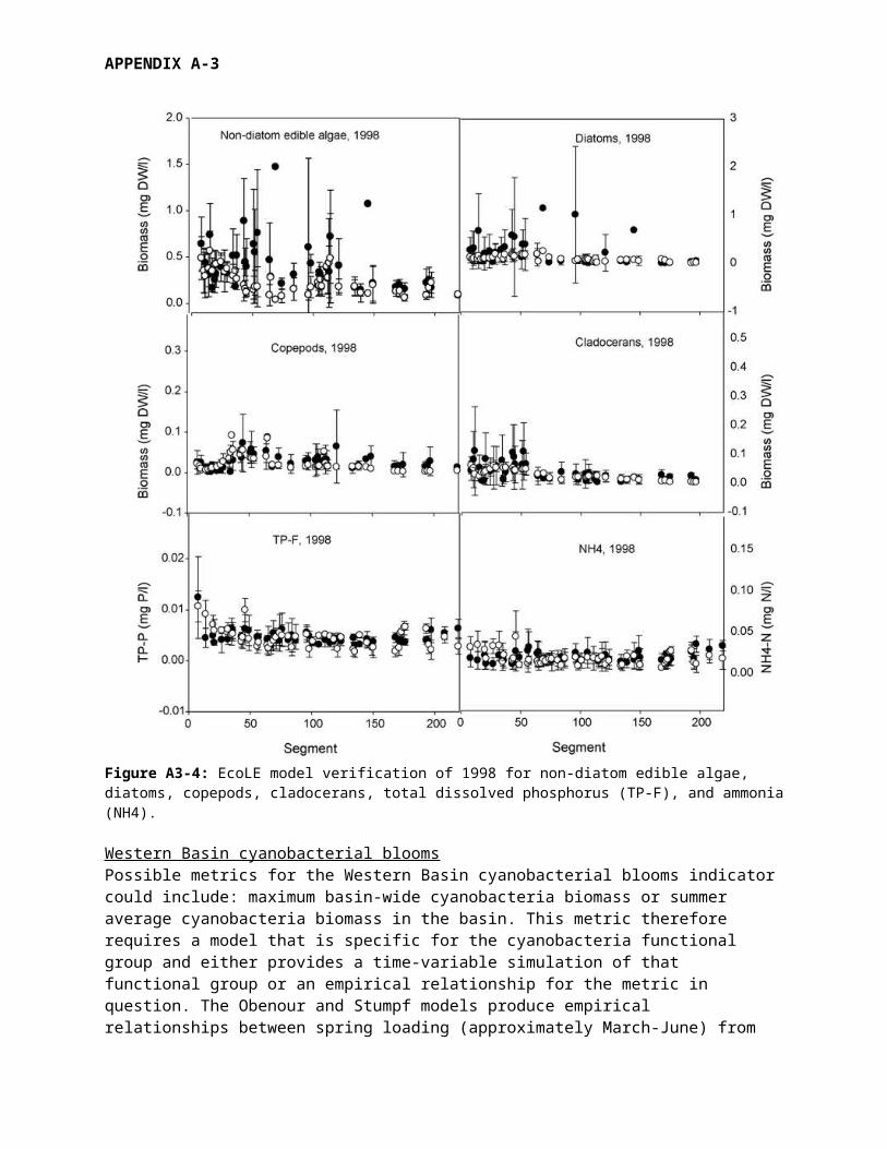
U-M/GLERL Western Lake Erie HAB Forecasting Model (Obenour)A probabilistic model was developed to relate the size of the western basin cyanobacteria bloom to spring phosphorus loading (Obenour et al., in review). The model is calibrated to multiple sets of bloom observations, from previous remote sensing and in situ sampling studies. A Bayesian hierarchical framework is used to accommodate the multiple observation datasets, and to allow for rigorous uncertainty quantification. Furthermore, a cross validation exercise demonstrates the model is robust and would be useful for providing probabilistic bloom forecasts (Figure A3-5). The deterministic form of the model suggests that there is a threshold loading value, below which the bloom remains at a baseline (i.e., background level). Above this threshold, bloom size increases proportionally to phosphorus load. Importantly, the model includes a temporal trend component indicating that this threshold has been decreasing over the study period (2002-2013), such that the lake is now significantly more susceptible to cyanobacteria blooms than it was a decade ago.

Figure A3-5: Predicted vs. Observed Bloom intensity (U-M/GLERL Western Lake Erie HAB model).

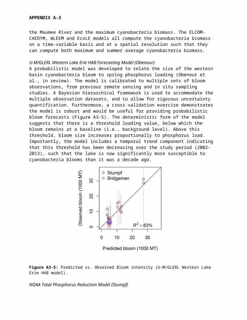
NOAA Total Phosphorus Reduction Model (Stumpf)In Stumpf et al. (2012) the authors present a regression between spring TP load and flow from the Maumee River and mean summer cyanobacteria index (CI) for western Lake Erie as calculated by the European space satellite, MERIS. This method applies an algorithm to convert raw satellite reflectance around the 681 nm band into an index that correlates with cyanobacteria density. Ten day composites were calculated by taking the maximum CI value at each pixel within a given 10-day period to remove clouds and capture areal biomass. The authors conclude that spring flow or TP load can be used to predict bloom magnitude. Average flow from March to June was the best predictor of CI utilizing data from 2002 to 2011 (Figure A3-6).

APPENDIX A-3

Figure A3-5: Maumee River TP load (March to June) versus cyanobacteria index (CI) from 2002 to 2011 (NOAA Total Phosphorus Reduction Model).

Western Lake Erie Ecosystem Model (WLEEM) (LimnoTech) (described above)

ELCOM-CAEDYM (Bocaniov ,Leon, and Yerubandi) (described above)

Ecological Model of Lake Erie - EcoLE (Zhang) (described above)

Central Basin hypoxiaPossible metrics for the Central Basin hypoxia indicator include the number of hypoxic days in the Central Basin during a given summer stratification period, and/or the average areal extent of the hypoxic zone during a given summer month, and/or the average hypolimnion DO concentration during the summer stratified period. The following existing models can provide estimates of the relationship between these metrics and external phosphorus loads.

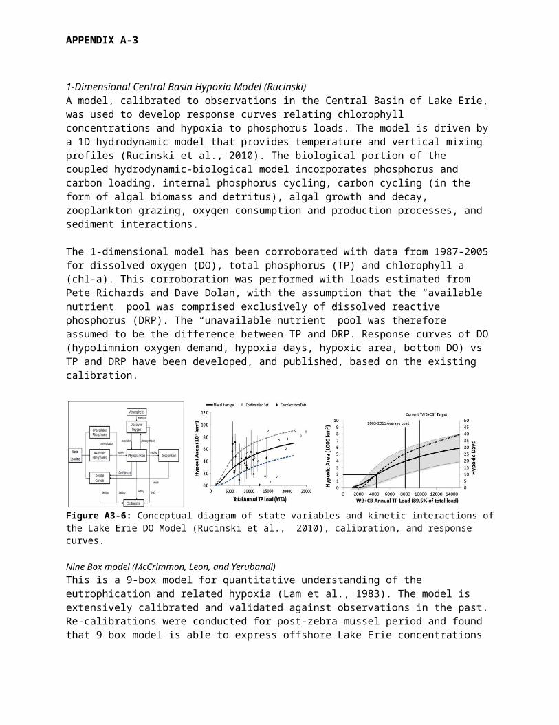
1-Dimensional Central Basin Hypoxia Model (Rucinski) A model, calibrated to observations in the Central Basin of Lake Erie, was used to develop response curves relating chlorophyll concentrations and hypoxia to phosphorus loads. The model is driven by a 1D hydrodynamic model that provides temperature and vertical mixing profiles (Rucinski et al., 2010). The biological portion of the coupled hydrodynamic-biological model incorporates phosphorus and carbon loading, internal phosphorus cycling, carbon cycling (in the form of algal biomass and detritus), algal growth and decay, zooplankton grazing, oxygen consumption and production processes, and sediment interactions.

The 1-dimensional model has been corroborated with data from 1987-2005 for dissolved oxygen (DO), total phosphorus (TP) and chlorophyll a (chl-a). This corroboration was performed with loads estimated from Pete Richards and Dave Dolan, with the assumption that the “available nutrient” pool was comprised exclusively of dissolved reactive phosphorus (DRP). The “unavailable nutrient” pool was therefore assumed to be the difference between TP and DRP. Response curves of DO (hypolimnion oxygen demand, hypoxia days, hypoxic area, bottom DO) vs TP and DRP have been developed, and published, based on the existing calibration.

APPENDIX A-3

Figure A3-6: Conceptual diagram of state variables and kinetic interactions of the Lake Erie DO Model (Rucinski et al., 2010), calibration, and response curves.

Nine Box model (McCrimmon, Leon, and Yerubandi)This is a 9-box model for quantitative understanding of the eutrophication and related hypoxia (Lam et al., 1983). The model is extensively calibrated and validated against observations in the past. Re-calibrations were conducted for post-zebra mussel period and found that 9 box model is able to express offshore Lake Erie concentrations reasonably well. The model can be expanded to include empirically derived chlorophyll relations for given TP concentrations.

Total Phosphorus Mass Balance Model (Chapra, Dolan, and Dove) (described above)The TP mass balance model is described in 3.1.1.

ELCOM-CAEDYM (Bocaniov ,Leon, and Yerubandi) (described above)

Ecological Model of Lake Erie - EcoLE (Zhang) (described above)

Eastern Basin Cladophora (nearshore) The indicator of concern for the Eastern Basin is Cladophora growth in nearshore areas. Here the two Cladophora growth models of Auer and Higgins are candidates for this analysis. Both models could provide estimates of biomass per unit area and areal coverage; however, both models require estimates of nearshore DRP concentrations. Those concentrations could potentially be provided by the ELCOM-CAEDYM (Leon/Bocaniov) model.

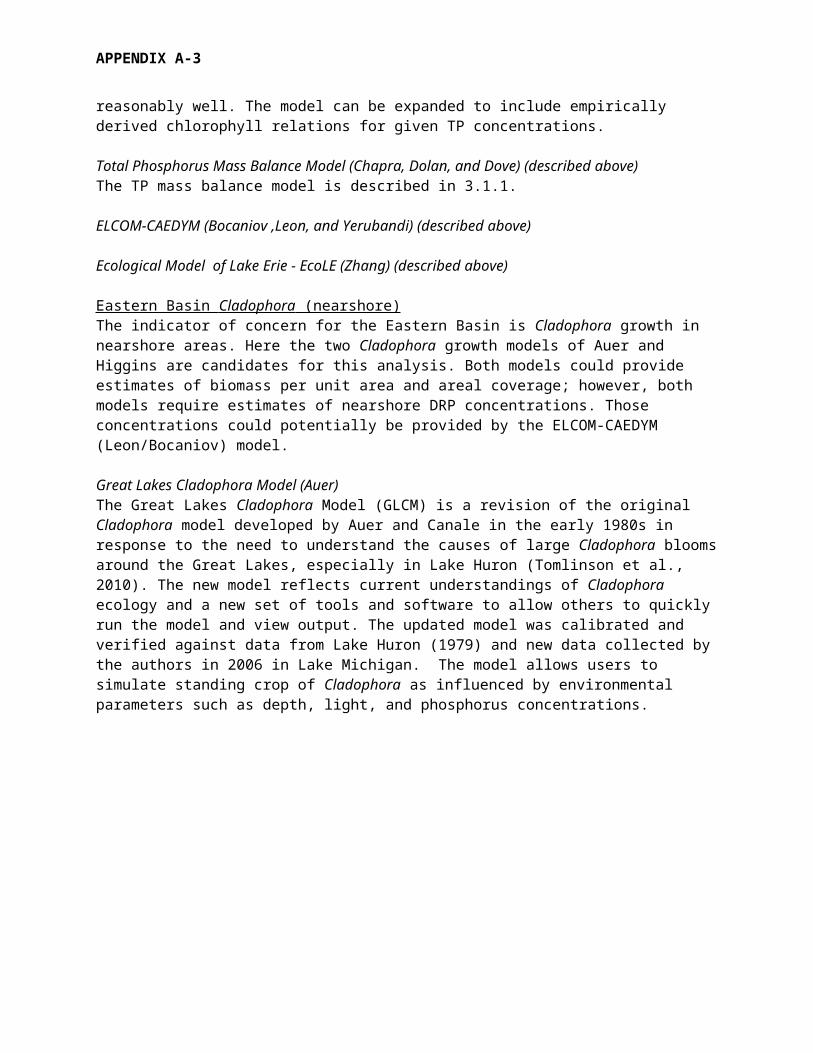
Great Lakes Cladophora Model (Auer)The Great Lakes Cladophora Model (GLCM) is a revision of the original Cladophora model developed by Auer and Canale in the early 1980s in response to the need to understand the causes of large Cladophora blooms around the Great Lakes, especially in Lake Huron (Tomlinson et al., 2010). The new model reflects current understandings of Cladophora ecology and a new set of tools and software to allow others to quickly run the model and view output. The updated model was calibrated and verified against data from Lake Huron (1979) and new data collected by the authors in 2006 in Lake Michigan. The model allows users to simulate standing crop of Cladophora as influenced by environmental parameters such as depth, light, and phosphorus concentrations.

APPENDIX A-3

Figure A3-7: Excerpt from Tomlinson et al. (2010) showing relationship between Cladophora biomass and ambient SRP concentration.

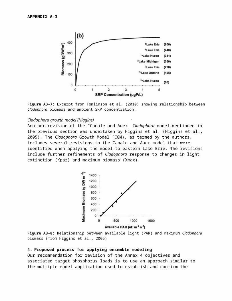
Cladophora growth model (Higgins)Another revision of the “Canale and Auer” Cladophora model mentioned in the previous section was undertaken by Higgins et al. (Higgins et al., 2005). The Cladophora Growth Model (CGM), as termed by the authors, includes several revisions to the Canale and Auer model that were identified when applying the model to eastern Lake Erie. The revisions include further refinements of Cladophora response to changes in light extinction (Kpar) and maximum biomass (Xmax).

Figure A3-8: Relationship between available light (PAR) and maximum Cladophora biomass (from Higgins et al., 2005)

4. Proposed process for applying ensemble modeling Our recommendation for revision of the Annex 4 objectives and associated target phosphorus loads is to use an approach similar to the multiple model application used to establish and confirm the target P loads in Annex 3 of the 1978 Amended GLWQA. The general philosophy is to begin with identifying the eutrophication response indicators (ERIs) of concern and to use multiple models to compute appropriate load-response relationships for each of the indicators. Then once the target/threshold measure of the eutrophication response indicators has been established, the load-response relationships can be used to compare and recommend loads corresponding to that threshold. Models that compute in-lake nutrient

APPENDIX A-3

concentrations along the way to producing the load-response relationship can potentially be used to extract the temporal and spatial profile of rivermouth, nearshore, and open-lake nutrient concentrations consistent with a given target load.

The ensemble of models proposed to be applied have all been developed to address the current Lake Erie ecosystem structure and function, including the potential to address both nearshore and offshore conditions. The models also represent a range of complexities and assumptions. This ensemble approach within which all models use the same basic input data (i.e., forcing functions) to create common load-response relationships provides several benefits over relying on a single model. First, by reconciling differences among results in terms of the different assumptions and model construction and parameterization, it provides insights into the most important sources and processes for a given system and management issue. Also, a given management question can be viewed from different conceptual and operational perspectives. The same datasets are mined in different ways. Multiple lines of evidence are compiled. All of this reduces the level of risk in environmental management decision-making. In the end, having great model diversity can add more value to the analysis than having a multiplicity of very similar models.

Short term effortsThe models capable of addressing each of these indicators have been identified and described briefly above. Each of those models will be applied using a series of tasks to produce a set of results to be used in making the target load and objectives recommendations. These tasks are described below.

Tasks required for each response indicator

Task 1: Define metrics (state variables) to be modeledEach modeling team will define the modeled metric/s (i.e., state variable) that will be computed to represent the ERIs that they are addressing (see metric descriptions above).

Task 2: Identify the models to be applied to each ERI Table A3-1 above lists five models to be used for the overall phytoplankton biomass ERI, five models to be used for the Western Basin cyanobacteria bloom ERI, five models to be used for the Central Basin hypoxia ERI, and a blending of two Cladophora models to be used for the Eastern Basin Cladophora ERI. Based on the workshop all of these models appear to be a valuable part of the multiple modeling effort to address the short-term Annex 4 goal stated above; however the final assessment will be made once individual model results are delivered (e.g., more complete documentation of response to the evaluation criteria outlined above). Each modeling effort will be required to provide the following information to serve as the basis for the final evaluation:

Complete documentation of model equations, coefficients, and driving variables Documented comparisons between model output and observations (state variables, processes)

used in calibration Documentation of post-calibration testing (e.g., comparison of model performance for

observations not used in the calibration) Documentation of formal and/or informal assessments of model uncertainty/sensitivity The response curves relating nutrient loads to the objective metrics.

Task 3: Apply models to develop load-response and other output analysesThis task describes the individual short-term activities that are planned for each of the models.

APPENDIX A-3

GeneralPrior to applying the models, a common (baseline) Lake Erie input data set needs to be developed for all models to have a common baseline input data set for their analysis. The proposed approach is to select a single year that contains the most complete representation of the necessary data and also represents a “typical” year with respect to such forcing functions as hydrology, wind, temperature, and Dreissenid densities. This year should come from the past 10 years or so of observations, so these conditions can be said to be “recent”. Then load alterations that might be analyzed in producing load-response curves would use all of the same inputs but simply adjust the concentration of phosphorus in the hydrologic inputs to the system.Possible years for developing this baseline are 2008, which according to Dolan and Chapra, is a good representation of average loading conditions to the lake. Another possibility would be 2013, which is a very recent year that provides conditions between the extreme western basin years of 2011 and 2012. We will collaborate with the Parties (EPA and EC) to produce data sets for both the input and in-lake response data for the selected common year.

The group will also decide on the suite of independent P load variables to use for the x-axis in the load-response analysis curves. These independent variable loads could have spatial and temporal specifications (e.g., basin loads, tributary loads, or seasonal loads) and they can have P form specifications (e.g., TP, DRP, Bioavailable P).

Total Phosphorus Mass Balance Model (Chapra, Dolan, and Dove)In the short term, this model would be used in its present version to develop basin-specific load-response curves for TP and chlorophyll a (Chapra and Dolan, 2012). Chapra would also investigate the feasibility of extending his model framework to compute hypolimnetic oxygen and sediment nutrient release in the Central Basin (Chapra and Canale, 1991).

ELCOM-CAEDYM (Bocaniov, Leon, and Yerubandi)In the short-term, Environment Canada and Bocaniov will collaborate to undertake the following ELCOM-CAEDYM model application activities:

1. Using the common, baseline year selected by the modeling group, assess ELCOM-CAEDYM performance with respect to observed nutrient and phytoplankton concentrations during that year.

2. Control experiments with different loading scenarios similar to those suggested for WLEEM.3. Generate Load (TP, SRP) vs Total Chl-a curves4. Generate Load (TP, SRP) vs Cyanobacteria Chl-a5. Generate Load (TP) vs Hypolimnetic oxygen concentration6. Generate Load (TP) vs hypoxia area

Nine Box model (McCrimmon, Leon, and Yerubandi)In the short-term, the Lam et al. 9-box model will also be applied by Environment Canada with the following steps:

1. Using the common, baseline year selected by the modeling group, assess 9 Box model performance with respect to observed nutrient during that year

2. Run NWRI vertical temperature model for providing stratification to hypoxia model3. Generate Load (TP) vs concentrations in west, central and east basins4. Generate Load (TP) vs DO concentrations5. Generate Load (TP) vs hypoxia area (NWRI method)

APPENDIX A-3

1-Dimensional Central Basin Hypoxia Model (Rucinski)This model can produce a range of hypoxia conditions (any of the selected metrics) for a given load as a function of a range of observed or hypothesized physical forcing conditions that might affect the duration and magnitude and depth of stratification. The short-term application will do the following steps:

Using the existing model parameterization and the common, baseline year a series of hypoxia load-response curves will be developed for the three metrics. These curves will be driven by the same load reduction scenarios suggested for the WLEEM model (applied to both the Western Basin and Central Basin inputs). The load of phosphorus and organic material from the Western Basin to the Central Basin for those scenarios will be computed by WLEEM.

Chlorophyll a load-response curves will be produced using the same series of P load reduction scenarios. This will provide an input to the overall phytoplankton biomass metric.

Using loads of phosphorus and oxygen-demanding material from the Western Basin based on WLEEM may require re-calibration/corroboration of the model prior to its application for the first two bullets above.

Ecological Model of Lake Erie - EcoLE (Zhang)The Zhang short term activities will first have to examine how to initialize and run the model for the common, baseline year. They will then check the model against total chlorophyll a, cyanobacteria chlorophyll a, and central basin DO for that year, and possibly recalibrate. The recalibrated model will then be used to generate load-response curves for total chlorophyll a in each basin, cyanobacteria biomass in the Western Basin, and hypoxia in the central basin.

Western Lake Erie Ecosystem Model (WLEEM) (LimnoTech)WLEEM will be run for the common baseline year using nutrient and solids loads to the Western Basin from all sources estimated in the same way that Dolan estimated the loads for the EcoFore project. The model will produce spatial and temporal profile outputs of TP, DRP, NO3, TNH3, TKN, total phytoplankton biomass (as mgC/L and chlorophyll a), functional phytoplankton group biomass (e.g., cyanobacteria), and several ancillary state variables (T, chloride, TSS and VSS, Ke, DO). The concentration of all state variable outputs will be expressible as either volumetric concentration in a given 3D model cell or as a depth averaged concentration for every horizontal grid cell. The state variables can also be expressed as a mass of the constituent in a given volume of water, thus facilitating the development of Western Basin mass balances from the model output. These mass balances can be developed on any spatial and temporal basis, including the total mass of cyanobacteria in the Western Basin integrated over the entire growing season. In summary, concentration or mass balance outputs can then be averaged or aggregated over any desired time and space (e.g., basinwide, August average of cyanobacteria chlorophyll a).

The following scenarios will be run with the model using the common baseline year (additional scenarios may be run based on suggestions from managers):

Baseline loads and flows and other forcing functions; Reduce TP and DRP loads (by reducing concentration) from all tributaries and the Detroit River

by 25%, 50%, 75%, 100%; Reduce TP and DRP loads (by reducing concentration) from only the Maumee River by 25%,

50%, 75%, 100%; Reduce TP and DRP loads (by reducing concentration) from only the Detroit River by 25%, 50%,

75%, 100%;

APPENDIX A-3

Reduce only DRP loads (by reducing concentration) from all tributaries and the Detroit River by 25%, 50%, 75%, 100%;

Reduce only DRP loads (by reducing concentration) from only the Maumee River by 25%, 50%, 75%, 100%;

Baseline with no sediment feedback, either by resuspension or pore water diffusion).

The output from these scenarios will permit the production of a large suite of load-response plots with TP or DRP load (either annual or cumulative over some specified time period, like March-June) on the x-axis and any one of the state variables on the y-axis (again averaged over any specified time and/or space designation for the Western Basin). The output will also be used to compute net fluxes (loads) of phosphorus and decomposable organic carbon to the Central Basin by various load management options.

U-M/GLERL Western Lake Erie HAB Forecasting Model (Obenour)In the short term, the application of the Obenour model will include the following steps:

1. Recalibrate model to ‘bioavailable’ phosphorus loads. Bioavailable phosphorus loads will be determined by applying ‘bioavailable fraction coefficients’ to the DRP and non-DRP phosphorus loads from the Maumee River. The coefficients will be initialized based on prior information developed through literature review, and the coefficients will be updated based on bloom model calibration, through Bayesian inference. This revise calibration will be compared with those generated using TP and DRP loads.

2. Expand scope of the model. The bloom forecasting model will be re-calibrated to an expanded dataset of harmful algal bloom observations, covering 1979-1987 and 1998-present. Observations prior to 2002 will be derived from SeaWiFs and CZCS satellite imagery. By expanding the calibration dataset, it will be possible to consider additional biophysical drivers of the temporal variability in harmful algal blooms. In addition to Maumee River nutrient loads, water column mixing, sea surface temperature, and Detroit River nutrient loads will be added to the analysis as potential bloom predictors. The resulting model will refine our understanding of the causes of cyanobacteria blooms, and may suggest new management measures, beyond Maumee River phosphorus load reductions.

NOAA Total Phosphorus Reduction Model (Stumpf)In the short term, Stumpf will apply their bloom severity forecasting model to suggest TP and DRP load targets using the Maumee River as the surrogate for the loading of influence in the western basin.

First, they will update the model published in Stumpf et al., 2012.Then they will produce load-response curves for the Western Basin cyanobacteria metrics using the revised model. The load-response plots will also provide estimates of uncertainty for the various relationships examined.

Great Lakes Cladophora Model (Auer) The modeling effort in the short-term will be to model the change in Cladophora biomass production in a model domain along the north shoreline of the Eastern Basin in response to changes in external loading to the lake under various loading scenarios. Specifically, this effort will include:

Adapt the Great Lakes Cladophora Model (GLCM, Tomlinson et al., 2010) to accommodate selected features of the Cladophora Growth Model (Higgins et al., 2005), the only other attached algae modeling tool presently available;

APPENDIX A-3

Perform sensitivity analyses with the GLCM to facilitate the assignment of uncertainty estimates to the P-loading/Cladophora response relationship;

Apply a whole lake modeling framework such as ELCOM-CAEDYM to establish the (spatiotemporal) phosphorus regime of the eastern basin for baseline and projected tributary and point source bioavailable P loads and for a range of bioavailable P concentrations at the eastern basin – central basin boundary;

Apply the GLCM to establish a load-response relationship between bioavailable P levels at the eastern basin – central basin boundary and Cladophora growth and estimates of uncertainty in the Cladophora response at each P level.

Task 4: Evaluation of deliverables against the criteriaThe modeling team will use the evaluation criteria outlined above and the deliverables from each group to assess which model results will be used in the ensemble.

Task 5: Conduct comparison analysis among models for each ERI For each ERI, load-response outputs will be compared among the models to identify significant differences and to understand those differences in terms of model formulation and inherent assumptions. A modeling group decision will be made on how to represent the various models in establishing a target load to meet a given ERI metric.

This task will also include, if appropriate, producing an in-lake nutrient concentration profile in space and time for each target load to demonstrate its variability and to stress the resources necessary to monitor compliance on that basis.

Task 6: Synthesize results and formulate recommended initial target loadsThis task would be accomplished in cooperation with the entire Annex 4 Objectives Task Group. The modeling sub-group will synthesize and document the results of the first five tasks with a sub-group meeting. Then the documented results will be shared with the entire Objectives Task Group and another face-to-face meeting will take place with the goal of developing a report to be sent forward to the Annex 4 Committee.

APPENDIX A-3

5. References

Bierman,V.J. 1980. A Comparison of Models Developed for Phosphorus Management in the Great Lakes. Conference on Phosphorus Management Strategies for the Great Lakes. pp. 1-38.

Bocaniov, S.A., Smith, R.E.H, Spillman, C.M., Hipsey, M.R., Leon, L.F., 2014. The nearshore shunt and the decline of the phytoplankton spring bloom in the Laurentian Great Lakes: insights from a three-dimensional lake model. Hydrobiol. 731, 151-172.

Chapra, S.C. and Canale, R.P., 1991. Long-Term Phenomenological Model of Phosphorus and Oxygen in Stratified Lakes. Water Research. 25(6):707-715.

Chapra, S.C., Dolan,D.M. 2012. Great Lakes total phosphorus revisited: 2. Mass balance modeling. J Great Lakes Res. Vol. 38 (4). pp. 741-754.

Conroy, J.D., Boegman, L., Zhang, H., Edwards, W.J., Culver, D.A. 2011. “Dead Zone” dynamics in Lake Erie: the importance of weather and sampling intensity for calculated hypolimnetic oxygen depletion rates. Aquatic Sciences. 73:289-304.

DePinto, J.V., Lam, D., Auer, M.T., Burns, N., Chapra, S.C., Charlton, M.N., Dolan, D.M., Kreis, R., Howell, T., Scavia, D. 2006. EXAMINATION OF THE STATUS OF THE GOALS OF ANNEX 3 OF THE GREAT LAKES WATER QUALITY AGREEMENT. Rockwell, D., VanBochove, E., Looby, T. (eds). pp. 1-31.

Higgins, S.N., Hecky, R.E., Guildford, S.J. 2005a. Modeling the Growth, Biomass, and Tissue Phosphorus Concentration of Cladophora glomerata in Eastern Lake Erie: Model Description and Field Testing. Journal of Great Lakes Research. Vol. 31. pp. 439-455.

Hipsey, M.R., Hamilton, D.P., 2008. Computational aquatic ecosystems dynamics model: CAEDYM v3 Science Manual. Centre for Water Research Report, University of Western Australia.

Lam, D.C.L., W.M. Schertzer and A.S. Fraser, 1983. Simulation of Lake Erie water quality responses to loading and weather conditions; Scientific Series. 134, National Water Research Insitute, Canada Centre for Inland Waters, Burlington, Canada.

Leon, L.F., Smith, R.E.H., Hipsey, M.R., Bocaniov, S.A., Higgins, S.N., Hecky, R.E., Antenucci, J.P., Imberger, J.A., Guildford, S.J. 2011. Application of a 3D hydrodynamic–biological model for seasonal and spatial dynamics of water quality and phytoplankton in Lake Erie. Journal of Great Lakes Research. Vol. 37. pp. 41-53.

Liu, W., Bocaniov, S.A., Lamb, K.G., Smith, R.E.H. Three dimensional modeling of the effects of changes in meteorological forcing on the thermal structure of Lake Erie. Journal of Great Lakes Research (in revision)

Oveisy, A., Rao, Y.R., Leon, L.F., Bocaniov, S.A. Three-dimensional winter modelling and the effects of ice cover on hydrodynamics, thermal structure and water quality in Lake Erie. Journal of Great Lakes Research (in final revision)

Rucinski, D.R., Beletsky, D., DePinto, J.V., Schwab, D.J., Scavia, D. 2010. A simple 1-dimensional, climate based dissolved oxygen model for the central basin of Lake Erie. Journal of Great Lakes Research. Vol. 36. pp. 465-476.

Stumpf, R.P., Wynne, T.T., Baker, D.B., Fahnenstiel, G.L. 2012. Interannual Variability of Cyanobacterial Blooms in Lake Erie. PLoS ONE. Vol. 7 (8). pp. 1-11.

Tomlinson, L.M., Auer, M.T., Bootsma, H.A., Owens, E.M. 2010. The Great Lakes Cladophora Model: Development, testing, and application to Lake Michigan. Journal of Great Lakes Research. Vol. 36. pp. 287-297.

United States and Canada 2012. 2012 Great Lakes Water Quality Agreement. USEPA and Environment Canada (ed). p. Annex 4. http://www.epa.gov/glnpo/glwqa/.

Vallentyne, J.R., Thomas, N.A. 1978. Fifth Year Review of Canada-United State Great Lakes Water Quality Agreement Report of Task Group III A Technical Group to Review Phosphorus Loadings. pp. 1-100.

APPENDIX A-3

Zhang, H., Culver, D.A., and Boegman, L. 2008. A Two-Dimensional Ecological Model of Lake Erie: Application to Estimate Dreissenid Impacts on Large Lake Plankton Populations. Ecological Modelling, 214: 219-241.

Zhang, H., Culver, D.A., Boegman, L. 2011. Dreissenids in Lake Erie: an algal filter or a fertilizer? Aquatic Invasions. Vol. 6 (2). pp. 175-194.