M.A. PREVIOUS ECONOMICS

PAPER IIIQUANATITATIVE METHODS

BLOCK 2

MATHEMATICAL METHODS

PAPER IIIQUANTITATIVE METHODS

BLOCK 2

MATHEMATICAL METHODS

CONTENTS

Unit 1 Basic concepts of linear Programming 4

Unit 2 Solutions to linear programming problems 12 And theory of game

2

BLOCK 2 MATHEMATICAL METHODS

This block consists of two units. The first unit deals with basic concepts of linear programming, its uses, forms, slackness and concepts related to duality. The second unit thoroughly discusses solutions to linear programming problems including optimal solution of linear programming through graphical method. The unit also throws light on concept of games, different strategies of game and the saddle point solution.

3

UNIT 1

BASIC CONCEPTS OF LINEAR PROGRAMMING

Objectives

After studying this unit you should be able to:

Understand the basic concept of Linear Programming Analyze the uses of Linear Programming

Know the different concepts of standard form and augmented form problems.

Have the knowledge of complementary slackness theorem

Structure

1.1 Introduction1.2 Uses of Linear Programming1.3 Standard form1.4 Augmented form1.5 Duality1.6 Special cases1.7 Complementary slackness1.8 Summary1.9 Further readings

1.1 INTRODUCTION

In mathematics, linear programming (LP) is a technique for optimization of a linear objective function, subject to linear equality and linear inequality constraints. Informally, linear programming determines the way to achieve the best outcome (such as maximum profit or lowest cost) in a given mathematical model and given some list of requirements represented as linear equations.

More formally, given a polytope (for example, a polygon or a polyhedron), and a real-valued affine function

defined on this polytope, a linear programming method will find a point in the polytope where this function has the smallest (or largest) value. Such points may not exist, but if they do, searching through the polytope vertices is guaranteed to find at least one of them.

4

Linear programs are problems that can be expressed in canonical form:

Maximize Subject to

X represents the vector of variables (to be determined), while c and b are vectors of (known) coefficients and A is a (known) matrix of coefficients. The expression to be maximized or minimized is called the objective function ( in this case). The equations

are the constraints which specify a convex polyhedron over which the objective function is to be optimized.

Linear programming can be applied to various fields of study. Most extensively it is used in business and economic situations, but can also be utilized for some engineering problems. Some industries that use linear programming models include transportation, energy, telecommunications, and manufacturing. It has proved useful in modeling diverse types of problems in planning, routing, scheduling, assignment, and design.

Theory

Geometrically, the linear constraints define a convex polyhedron, which is called the feasible region. Since the objective function is also linear, hence a convex function, all local optima are automatically global optima (by the KKT theorem). The linearity of the objective function also implies that the set of optimal solutions is the convex hull of a finite set of points - usually a single point.

There are two situations in which no optimal solution can be found. First, if the constraints contradict each other (for instance, x ≥ 2 and x ≤ 1) then the feasible region is empty and there can be no optimal solution, since there are no solutions at all. In this case, the LP is said to be infeasible.

Alternatively, the polyhedron can be unbounded in the direction of the objective function (for example: maximize x1 + 3 x2 subject to x1 ≥ 0, x2 ≥ 0, x1 + x2 ≥ 10), in which case there is no optimal solution since solutions with arbitrarily high values of the objective function can be constructed.

Barring these two pathological conditions (which are often ruled out by resource constraints integral to the problem being represented, as above), the optimum is always attained at a vertex of the polyhedron. However, the optimum is not necessarily unique: it is possible to have a set of optimal solutions covering an edge or face of the polyhedron, or even the entire polyhedron (This last situation would occur if the objective function were constant).

1.2 USES OF LINEAR PROGRAMMING

5

Linear programming is a considerable field of optimization for several reasons. Many practical problems in operations research can be expressed as linear programming problems. Certain special cases of linear programming, such as network flow problems and multicommodity flow problems are considered important enough to have generated much research on specialized algorithms for their solution. A number of algorithms for other types of optimization problems work by solving LP problems as sub-problems. Historically, ideas from linear programming have inspired many of the central concepts of optimization theory, such as duality, decomposition, and the importance of convexity and its generalizations. Likewise, linear programming is heavily used in microeconomics and company management, such as planning, production, transportation, technology and other issues. Although the modern management issues are ever-changing, most companies would like to maximize profits or minimize costs with limited resources. Therefore, many issues can boil down to linear programming problems.

1.3 STANDARD FORM

Standard form is the usual and most intuitive form of describing a linear programming problem. It consists of the following three parts:

A linear function to be maximized

e.g. maximize Problem constraints of the following form

e.g.

Non-negative variables

e.g.

The problem is usually expressed in matrix form, and then becomes:

maximize subject to

Other forms, such as minimization problems, problems with constraints on alternative forms, as well as problems involving negative variables can always be rewritten into an equivalent problem in standard form.

Example 1

Suppose that a farmer has a piece of farm land, say A square kilometres large, to be planted with either wheat or barley or some combination of the two. The farmer has a

6

limited permissible amount F of fertilizer and P of insecticide which can be used, each of which is required in different amounts per unit area for wheat (F1, P1) and barley (F2, P2). Let S1 be the selling price of wheat, and S2 the price of barley. If we denote the area planted with wheat and barley by x1 and x2 respectively, then the optimal number of square kilometres to plant with wheat vs barley can be expressed as a linear programming problem:

maximize (maximize the revenue — revenue is the "objective function")

subject to (limit on total area)(limit on fertilizer)(limit on insecticide)(cannot plant a negative area)

Which in matrix form becomes:

maximize

subject to

1.4 AUGMENTED FORM (SLACK FORM)

Linear programming problems must be converted into augmented form before being solved by the simplex algorithm. This form introduces non-negative slack variables to replace inequalities with equalities in the constraints. The problem can then be written in the following form:

Maximize Z in:

where are the newly introduced slack variables, and Z is the variable to be maximized.

Example 2

The example above becomes as follows when converted into augmented form:

maximize (objective function)subject to (augmented constraint)

(augmented constraint)(augmented constraint)

7

where are (non-negative) slack variables.

Which in matrix form becomes:

Maximize Z   in:

1.5 DUALITY

Every linear programming problem, referred to as a primal problem, can be converted into a dual problem, which provides an upper bound to the optimal value of the primal problem. In matrix form, we can express the primal problem as:

maximize subject to

The corresponding dual problem is:

minimize subject to

where y is used instead of x as variable vector.

There are two ideas fundamental to duality theory. One is the fact that the dual of a dual linear program is the original primal linear program. Additionally, every feasible solution for a linear program gives a bound on the optimal value of the objective function of its dual. The weak duality theorem states that the objective function value of the dual at any feasible solution is always greater than or equal to the objective function value of the primal at any feasible solution. The strong duality theorem states that if the primal has an optimal solution, x*, then the dual also has an optimal solution, y*, such that cTx*=bTy*.

A linear program can also be unbounded or infeasible. Duality theory tells us that if the primal is unbounded then the dual is infeasible by the weak duality theorem. Likewise, if the dual is unbounded, then the primal must be infeasible. However, it is possible for both the dual and the primal to be infeasible (See also Farkas' lemma).

Example 3

8

Revisit the above example of the farmer who may grow wheat and barley with the set provision of some A land, F fertilizer and P insecticide. Assume now that unit prices for each of these means of production (inputs) are set by a planning board. The planning board's job is to minimize the total cost of procuring the set amounts of inputs while providing the farmer with a floor on the unit price of each of his crops (outputs), S1 for wheat and S2 for barley. This corresponds to the following linear programming problem:

minimize (minimize the total cost of the means of production as the "objective function")

subject to (the farmer must receive no less than S1 for his wheat)

(the farmer must receive no less than S2 for his barley)(prices cannot be negative)

Which in matrix form becomes:

minimize

subject to

The primal problem deals with physical quantities. With all inputs available in limited quantities, and assuming the unit prices of all outputs is known, what quantities of outputs to produce so as to maximize total revenue? The dual problem deals with economic values. With floor guarantees on all output unit prices, and assuming the available quantity of all inputs is known, what input unit pricing scheme to set so as to minimize total expenditure?

To each variable in the primal space corresponds an inequality to satisfy in the dual space, both indexed by output type. To each inequality to satisfy in the primal space corresponds a variable in the dual space, both indexed by input type.

The coefficients which bound the inequalities in the primal space are used to compute the objective in the dual space, input quantities in this example. The coefficients used to compute the objective in the primal space bound the inequalities in the dual space, output unit prices in this example.

Both the primal and the dual problems make use of the same matrix. In the primal space, this matrix expresses the consumption of physical quantities of inputs necessary to produce set quantities of outputs. In the dual space, it expresses the creation of the economic values associated with the outputs from set input unit prices.

9

Since each inequality can be replaced by an equality and a slack variable, this means each primal variable corresponds to a dual slack variable, and each dual variable corresponds to a primal slack variable. This relation allows us to complementary slackness.

1.6 SPECIAL CASES

A packing LP is a linear program of the form

maximize subject to

such that the matrix A and the vectors b and c are non-negative.

The dual of a packing LP is a covering LP, a linear program of the form

minimize subject to

such that the matrix A and the vectors b and c are non-negative.

Example 4

Covering and packing LPs commonly arise as a linear programming relaxation of a combinatorial problem. For example, the LP relaxation of set packing problem, independent set problem, or matching is a packing LP. The LP relaxation of set cover problem, vertex cover problem, or dominating set problem is a covering LP.

Finding a fractional coloring of a graph is another example of a covering LP. In this case, there is one constraint for each vertex of the graph and one variable for each independent set of the graph.

1.7 COMPLEMENTARY SLACKNESS

It is possible to obtain an optimal solution to the dual when only an optimal solution to the primal is known using the complementary slackness theorem. The theorem states:

Suppose that x = (x1, x2, . . ., xn) is primal feasible and that y = (y1, y2, . . . , ym) is dual feasible. Let (w1, w2, . . ., wm) denote the corresponding primal slack variables, and let (z1, z2, . . . , zn) denote the corresponding dual slack variables. Then x and y are optimal for their respective problems if and only if xjzj = 0, for j = 1, 2, . . . , n, wiyi = 0, for i = 1, 2, . . . , m.

So if the ith slack variable of the primal is not zero, then the ith variable of the dual is equal zero. Likewise, if the jth slack variable of the dual is not zero, then the jth variable of the primal is equal to zero.

10

Activity 1

1. Discuss the uses of Linear Programming.2. Explain briefly the concept of Duality.

1.8 SUMMARY

Linear programming is an important field of optimization for several reasons. Many practical problems in operations research can be expressed as linear programming problems. Followed by the basic concept the concepts of duality, standard form and augmented form have described in the chapter.The different kind of problems can be solved using Linear Programming approach is discussed in special case section. Further the theorem of Complementary slackness was discussed in brief to have more clear understanding of solution to Linear programming problems.

1.9 FURTHER READINGS

Mark de Berg, Marc van Kreveld, Mark Overmars, and Otfried Schwarzkopf (2000). Computational Geometry (2nd revised edition ed.). Springer-Verlag.

V. Chandru and M.R.Rao, Linear Programming, Chapter 31 in Algorithms and Theory of Computation Handbook, edited by M.J.Atallah, CRC Press

V. Chandru and M.R.Rao, Integer Programming, Chapter 32 in Algorithms and Theory of Computation Handbook, edited by M.J.Atallah,

Thomas H. Cormen, Charles E. Leiserson, Ronald L. Rivest, and Clifford Stein. Introduction to Algorithms, Second Edition. MIT Press and McGraw-Hill

11

UNIT 2

SOLUTIONS TO LINEAR PROGRAMMING PROBLEMS AND THEORY OF GAME

Objectives

After studying this unit you should be able to:

Understand the basic concepts of computation of linear programming problems. Know the approaches to solve prototype and general linear programming

problems.

Solve the linear programming problems using graphical method.

Appreciate the concept and strategies pertaining to game theory.

Be aware about the saddle point solution.

Structure

2.1 Introduction2.2 Prototype LP Problem2.3 General LP problem2.4 Optimal solution through graphical method2.5 Concept of game2.6 Game strategies2.7 The saddle point solution2.8 Summary2.9 Further readings

2.1 INTRODUCTION

A Linear Programming problem is a special case of a Mathematical Programming problem. From an analytical perspective, a mathematical program tries to identify an

extreme (i.e., minimum or maximum) point of a function , which

furthermore satisfies a set of constraints, e.g., . Linear programming is the specialization of mathematical programming to the case where both, function f - to be called the objective function - and the problem constraints are linear.

Solution procedure used when a Linear Programming (LP) problem has two (or at most three) decision variables. The graphical method follows these steps:

(1) Change inequalities to equalities.

12

(2) Graph the equalities.

(3) Identify the correct side for the original inequalities.

(4) Then identify the feasible region, the area of Feasible Solution.

(5) Determine the Contribution Margin (CM) or cost at each of the corner points (basic feasible solutions) of the feasible region.

(6) Pick either the most profitable or least cost combination, which is an Optimal Solution.

2.2 A PROTOTYPE LP PROBLEM

Consider a company which produces two types of products P1 and P2 . Production of these products is supported by two workstations W1 and W2 , with each station visited by both product types. If workstation W1 is dedicated completely to the production of product type P1, it can process 40 units per day, while if it is dedicated to the production of product P2, it can process 60 units per day. Similarly, workstation W2 can produce daily 50 units of product P1 and 50 units of product P2 , assuming that it is dedicated completely to the production of the corresponding product. If the company's profit by disposing one unit of product P1 is $200 and that of disposing one unit of P2 is $400, and assumning that the company can dispose its entire production, how many units of each product should the company produce on a daily basis to maximize its profit?

Solution: First notice that this problem is an optimization problem. Our objective is to maximize the company's profit, which under the problem assumptions, is equivalent to maximizing the company's daily profit. Furthermore, we are going to maximize the company profit by adjusting the levels of the daily production for the two items P1 and P2 . Therefore, these daily production levels are the control/decision factors, the values of which we are called to determine. In the analytical formulation of the problem, the role of these factors is captured by modeling them as the problem decision variables:

X1 := number of units of product P1 to be produced daily X2:= number of units of product P2 to be produced daily

In the light of the above discussion, the problem objective can be expressed analytically as:

 

Equation 1 will be called the objective function of the problem, and the coefficients 200 and 400 which multiply the decision variables in it, will be called the objective function coefficients.

13

Furthermore, any decision regarding the daily production levels for items P1 and P2 in order to be realizable in the company's operation context must observe the production capacity of the two worksations W1 and W2 . Hence, our next step in the problem formulation seeks to introduce these technological constraints in it. Let's focus first on the constraint which expresses the finite production capacity of workstation W1 . Regarding this constraint, we know that one day's work dedicated to the production of item P1 can result in 40 units of that item, while the same period dedicated to the production of item P2 will provide 60 units of it. Assuming that production of one unit of product type Pi,i=1,2 requires a constant amount of processing time at workstation W1 ,

it follows that: and . Under the further assumption that the combined production of both items has no side-effects, i.e., does not impose any additional requirements for production capacity of workstation W1(e.g., zero set-up times), the total capacity (in terms of time length) required for producing X1units of product P1and X2

units of product P2 is equal to . Hence, the technological constraint imposing the condition that our total daily processing requirements for workstation W1 should not exceed its production capacity, is analytically expressed by:

 

Notice that in Equation 2 time is measured in days.

Following the same line of reasoning (and under similar assumptions), the constraint expressing the finite processing capacity of workstation is given by:

 

Constraints 2 and 3 are known as the technological constraints of the problem. In

particular, the coefficients of the variables in them, , are known as the technological coefficients of the problem formulation, while the values on the right-hand-side of the two inequalities define the right-hand side (rhs) vector of the constraints.

Finally, to the above constraints we must add the requirement that any permissible value for variables must be nonnegative, i.e.,

 

since these values express production levels. These constraints are known as the variable sign restrictions.

Combining Equations 1 to 4, the analytical formulation of our problem is as follows:

14

2.3 THE GENERAL LP FORMULATION

Generalizing formulation 5, the general form for a Linear Programming problem is as follows:

Objective Function:

 

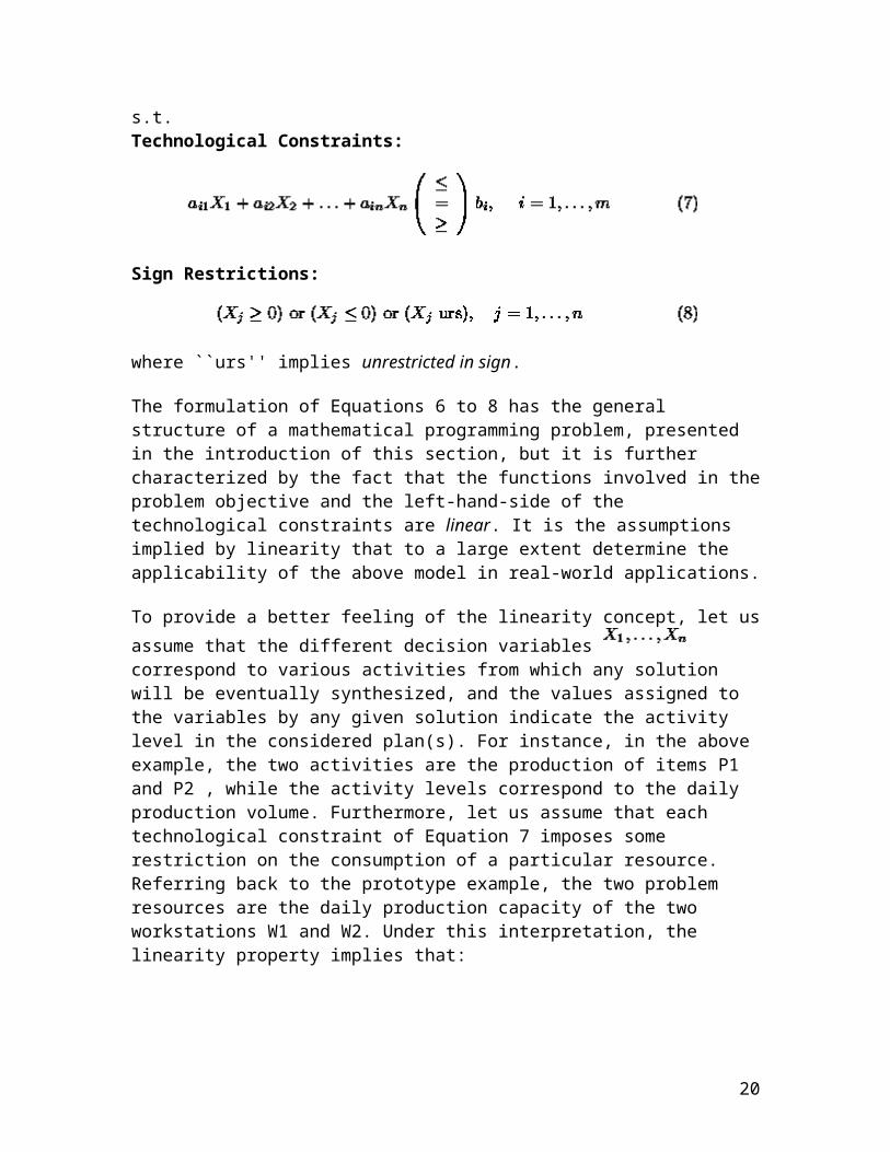
s.t. Technological Constraints:

 

Sign Restrictions:

 

where ``urs'' implies unrestricted in sign.

The formulation of Equations 6 to 8 has the general structure of a mathematical programming problem, presented in the introduction of this section, but it is further characterized by the fact that the functions involved in the problem objective and the left-hand-side of the technological constraints are linear. It is the assumptions implied by linearity that to a large extent determine the applicability of the above model in real-world applications.

To provide a better feeling of the linearity concept, let us assume that the different decision variables correspond to various activities from which any solution will be eventually synthesized, and the values assigned to the variables by any given solution indicate the activity level in the considered plan(s). For instance, in the above example, the two activities are the production of items P1 and P2 , while the activity levels correspond to the daily production volume. Furthermore, let us assume that each technological constraint of Equation 7 imposes some restriction on the consumption of a particular resource. Referring back to the prototype example, the two problem resources are the daily production capacity of the two workstations W1 and W2. Under this interpretation, the linearity property implies that:

15

Additivity assumption: the total consumption of each resource, as well as the overall objective value are the aggregates of the resource consumptions and the contributions to the problem objective, resulting by carrying out each activity independently, and

Proportionality assumption: these consumptions and contributions for each activity are proportional to the actual activity level.

It is interesting to notice how the above statement reflects to the logic that was applied when we derived the technological constraints of the prototype example: (i) Our assumption that the processing of each unit of product at every station requires a constant amount of time establishes the proportionality property for our model. (ii) The assumption that the total processing time required at every station to meet the production levels of both products is the aggregate of the processing times required for each product if the corresponding activity took place independently, implies that our system has an additive behavior. It is also interesting to see how the linearity assumption restricts the modeling capabilities of the LP framework: As an example, in the LP paradigm, we cannot immediately model effects like economies of scale in the problem cost structure, and/or situations in which resource consumption by one activity depends on the corresponding consumption by another complementary activity. In some cases, one can approach these more complicated problems by applying some linearization scheme. The resulting approximations for many of these cases have been reported to be quite satisfactory.

Another approximating element in many real-life LP applications results from the so called divisibility assumption. This assumption refers to the fact that for LP theory and algortihms to work, the problem variables must be real. However, in many LP formulations, meaningful values for the levels of the activities involved can be only integer. This is, for instance, the case with the production of items and in our prototype example. Introducing integrality requirements for some of the variables in an LP formulation turns the problem to one belonging in the class of (Mixed) Integer Programming (MIP). The complexity of a MIP problem is much higher than that of LP's. Actually, the general IP formulation has be shown to belong to the notorious class of NP-complete problems. (This is a class of problems that have been ``formally'' shown to be extremely ``hard'' computationally). Given the increased difficulty of solving IP problems, sometimes in practice, near optimal solutions are obtained by solving the LP formulation resulting by relaxing the integrality requirements - known as the LP relaxation of the corresponding IP - and (judiciously) rounding off the fractional values for the integral variables in the optimal solution. Such an approach can be more easily justified in cases where the typical values for the integral variables are in the order of tens or above, since the errors introduced by the rounding-off are rather small, in a relative sense.

16

We conclude our discussion on the general LP formulation, by formally defining the solution search space and optimality. Specifically, we shall define as the feasible region

of the LP of Equations 6 to 8, the entire set of vectors that satisfy the technological constraints of Eq. 7 and the sign restrictions of Eq. 8. An optimal solution to the problem is any feasible vector that further satisfies the optimality requirement expressed by Eq. 6. In the next section, we provide a geometric characterization of the feasible region and the optimality condition, for the special case of LP's having only two decision variables.

2.4 OPTIMAL SOLUTION THROUGH GRAPHICAL METHOD

This section develops a solution approach for LP problems, which is based on a geometrical representation of the feasible region and the objective function. In particular, the space to be considered is the n-dimensional space with each dimension defined by one of the LP variables Xj . The objective function will be described in this n-dim space by its contour plots, i.e., the sets of points that correspond to the same objective value. To the extent that the proposed approach requires the visualization of the underlying geometry, it is applicable only for LP's with upto three variables. Actually, to facilitate the visualization of the concepts involved, in this section we shall restrict ourselves to the two-dimensional case, i.e., to LP's with two decision variables. In the next section, we shall generalize the geometry introduced here for the 2-var case, to the case of LP's with n decision variables, providing more analytic (algebraic) characterizations of these concepts and properties.

Graphical solution of the prototype example 1: 2-var LP with a unique optimal solution

The `` sliding motion'' described suggests a way for identifying the optimal values for, let's say, a max LP problem. The underlying idea is to keep ``sliding'' the isoprofit line

in the direction of increasing 's, until we cross the boundary of the LP feasible region. The implementation of this idea on the prototype LP of Equation 5 is depicted in Figure 3.

17

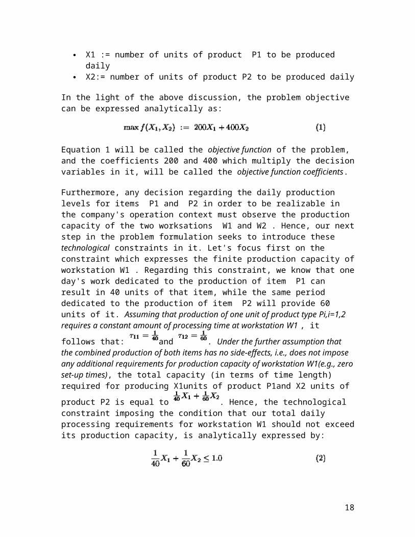
   Figure 2.1: Graphical solution of the prototype example LP

From this figure, it follows that the optimal daily production levels for the protoype LP are given by the coordinates of the point corresponding to the intersection of line

with the -axis, i.e., . The maximal daily profit

is . Notice that the optimal point is one of the ``corner'' points of the feasible region depicted in Figure 3. Can you argue that for the geometry of the feasible region for 2-var LP's described above, if there is a bounded optimal solution, then there will be one which corresponds to one of the corner points? (This argument is developed for the broader context of n-var LP's in the next section.)

2-var LP's with many optimal solutions

Consider our prototype example with the unit profit of item being $600 instead of $200. Under this modification, the problem isoprofit lines become:

and they are parallel to the line corresponding to the first problem constraint:

Therefore, if we try to apply the optimizing technique of the previous paragraph in this case, we get the situation depicted below (Figure 4), i.e., every point in the line segment CD is an optimal point, providing the optimal objective value of $24,000.

18

   Figure 2.2 : An LP with many optimal solutions

It is worth-noticing that even in this case of many optimal solutions, we have two of them corresponding to ``corner'' points of the feasible region, namely points C and D.

2.5 CONCEPT OF A GAME

Game theory attempts to mathematically capture behavior in strategic situations, in which an individual's success in making choices depends on the choices of others. While initially developed to analyze competitions in which one individual does better at another's expense (zero sum games), it has been expanded to treat a wide class of interactions, which are classified according to several criteria. Today, "game theory is a sort of umbrella or 'unified field' theory for the rational side of social science, where 'social' is interpreted broadly, to include human as well as non-human players (computers, animals, plants)" (Aumann 1987).

Representation of games

The games studied in game theory are well-defined mathematical objects. A game consists of a set of players, a set of moves (or strategies) available to those players, and a specification of payoffs for each combination of strategies. Most cooperative games are presented in the characteristic function form, while the extensive and the normal forms are used to define noncooperative games.

Extensive formMain article: Extensive form game

19

An extensive form game

The extensive form can be used to formalize games with some important order. Games here are often presented as trees (as pictured to the left). Here each vertex (or node) represents a point of choice for a player. The player is specified by a number listed by the vertex. The lines out of the vertex represent a possible action for that player. The payoffs are specified at the bottom of the tree.

In the game pictured here, there are two players. Player 1 moves first and chooses either F or U. Player 2 sees Player 1's move and then chooses A or R. Suppose that Player 1 chooses U and then Player 2 chooses A, then Player 1 gets 8 and Player 2 gets 2.

The extensive form can also capture simultaneous-move games and games with imperfect information. To represent it, either a dotted line connects different vertices to represent them as being part of the same information set (i.e., the players do not know at which point they are), or a closed line is drawn around them.

Normal form

The normal (or strategic form) game is usually represented by a matrix which shows the players, strategies, and payoffs (see the example to the right). More generally it can be represented by any function that associates a payoff for each player with every possible combination of actions. In the accompanying example there are two players; one chooses the row and the other chooses the column. Each player has two strategies, which are specified by the number of rows and the number of columns. The payoffs are provided in the interior. The first number is the payoff received by the row player (Player 1 in our example); the second is the payoff for the column player (Player 2 in our example). Suppose that Player 1 plays Up and that Player 2 plays Left. Then Player 1 gets a payoff of 4, and Player 2 gets 3.

When a game is presented in normal form, it is presumed that each player acts simultaneously or, at least, without knowing the actions of the other. If players have some information about the choices of other players, the game is usually presented in extensive form.

Characteristic function formMain article: Cooperative game

Player 2chooses Left

Player 2chooses Right

Player 1chooses Up 4, 3 –1, –1

Player 1chooses Down 0, 0 3, 4

Normal form or payoff matrix of a 2-player, 2-strategy game

20

In cooperative games with transferable utility no individual payoffs are given. Instead, the characteristic function determines the payoff of each coalition. The standard assumption is that the empty coalition obtains a payoff of 0.

The origin of this form is to be found in the seminal book of von Neumann and Morgenstern who, when studying coalitional normal form games, assumed that when a coalition C forms, it plays against the complementary coalition ( ) as if they were playing a 2-player game. The equilibrium payoff of C is characteristic. Now there are different models to derive coalitional values from normal form games, but not all games in characteristic function form can be derived from normal form games.

Formally, a characteristic function form game (also known as a TU-game) is given as a pair (N,v), where N denotes a set of players and is a characteristic function.

The characteristic function form has been generalised to games without the assumption of transferable utility.

Partition function form

The characteristic function form ignores the possible externalities of coalition formation. In the partition function form the payoff of a coalition depends not only on its members, but also on the way the rest of the players are partitioned (Thrall & Lucas 1963).

2.6 GAME STRATEGIES

The particular behavior or suite of behaviors that a player uses is termed a strategy (see important note). Strategies can be behaviors that are on some continuum (e.g., how long to wait or display) or they may represent discrete behavior types (e.g., display, fight, or flee). Sometimes the terms pure strategy and mixed strategy are used.

A simple or pure strategy provides a complete definition of how a player will play a game. In particular, it determines the move a player will make for any situation they could face. A player's strategy set is the set of pure strategies available to that player. A pure strategy in fact, is a strategy that is not defined in terms of other strategies present in the game.

A mixed strategy is an assignment of a probability to each pure strategy. This allows for a player to randomly select a pure strategy. Since probabilities are continuous, there are infinitely many mixed strategies available to a player, even if their strategy set is finite.

Mixed strategy

21

Suppose the payoff matrix pictured to the right (known as a coordination game). Here one player chooses the row and the other chooses a column. The row player receives the first payoff, the column the second. If row opts to play A with probability 1 (i.e. play A for sure), then he is said to be playing a pure strategy. If column opts to flip a coin and play A if the coin lands heads and B if the coin lands tails, then she is said to be playing a mixed strategy, and not a pure strategy.

Significance

In his famous paper John Forbes Nash proved that there is an equilibrium for every finite game. One can divide Nash equilibria into two types. Pure strategy Nash equilibria are Nash equilibria where all players are playing pure strategies. Mixed strategy Nash equilibria are equilibria where at least one player is playing a mixed strategy. While Nash proved that every finite game has a Nash equilibrium, not all have pure strategy Nash equilibria. For an example of a game that does not have a Nash equilibrium in pure strategies see Matching pennies. However, many games do have pure strategy Nash equilibria (e.g. the Coordination game, the Prisoner's dilemma, the Stag hunt). Further, games can have both pure strategy and mixed strategy equilibria.

The Nash equilibrium concept is used to analyze the outcome of the strategic interaction of several decision makers. In other words, it is a way of predicting what will happen if several people or several institutions are making decisions at the same time, and if the decision of each one depends on the decisions of the others. The simple insight underlying John Nash's idea is that we cannot predict the result of the choices of multiple decision makers if we analyze those decisions in isolation. Instead, we must ask what each player would do, taking into account the decision-making of the others.

Formal definition

Let (S, f) be a game with n players, where Si is the strategy set for player i, S=S1 X S2 ... X Sn is the set of strategy profiles and f=(f1(x), ..., fn(x)) is the payoff function. Let x − i be a strategy profile of all players except for player i. When each player i {1, ..., n} chooses strategy xi resulting in strategy profile x = (x1, ..., xn) then player i obtains payoff fi(x). Note that the payoff depends on the strategy profile chosen, i.e. on the strategy chosen by player i as well as the strategies chosen by all the other players. A strategy profile x* S is a Nash equilibrium (NE) if no unilateral deviation in strategy by any single player is profitable for that player, that is

A game can have a pure strategy NE or an NE in its mixed extension (that of choosing a pure strategy stochastically with a fixed frequency). Nash proved that if we allow mixed strategies, then every n-player game in which every player can choose from finitely many strategies admits at least one Nash equilibrium.

A B

A 1, 1 0, 0

B 0, 0 1, 1

Pure coordination game

22

When the inequality above holds strictly (with > instead of ) for all players and all feasible alternative strategies, then the equilibrium is classified as a strict Nash equilibrium. If instead, for some player, there is exact equality between and some other strategy in the set S, then the equilibrium is classified as a weak Nash equilibrium.

Coordination game

Player 2 adopts strategy A

Player 2 adopts strategy B

Player 1 adopts strategy A 4, 4 1, 3

Player 1 adopts strategy B 3, 1 3, 3

A sample coordination game showing relative payoff for player1 / player2 with each combination

The coordination game is a classic (symmetric) two player, two strategy game, with an example payoff matrix shown to the right. The players should thus coordinate, both adopting strategy A, to receive the highest payoff, i.e., 4. If both players chose strategy B though, there is still a Nash equilibrium. Although each player is awarded less than optimal payoff, neither player has incentive to change strategy due to a reduction in the immediate payoff (from 3 to 1). An example of a coordination game is the setting where two technologies are available to two firms with compatible products, and they have to elect a strategy to become the market standard. If both firms agree on the chosen technology, high sales are expected for both firms. If the firms do not agree on the standard technology, few sales result. Both strategies are Nash equilibria of the game.

Driving on a road, and having to choose either to drive on the left or to drive on the right of the road, is also a coordination game. For example, with payoffs 100 meaning no crash and 0 meaning a crash, the coordination game can be defined with the following payoff matrix:

In this case there are two pure strategy Nash equilibria, when both choose to either drive on the left or on the right. If we admit mixed strategies (where a pure strategy is chosen at random, subject to some fixed probability),

then there are three Nash equilibria for the same case: two we have seen from the pure-strategy form, where the probabilities are (0%,100%) for player one, (0%, 100%) for player two; and (100%, 0%) for player one, (100%, 0%) for player two respectively. We add another where the probabilities for each player is (50%, 50%).

Drive on the Left Drive on the Right

Drive on the Left 100, 100 0, 0

Drive on the Right 0, 0 100, 100

The driving game

23

2.7 THE SADDLE POINT SOLUTION

a saddle point is a point in the domain of a function of two variables which is a stationary point but not a local extremum. At such a point, in general, the surface resembles a saddle that curves up in one direction, and curves down in a different direction (like a mountain pass). In terms of contour lines, a saddle point can be recognized, in general, by a contour that appears to intersect itself. For example, two hills separated by a high pass will show up a saddle point, at the top of the pass, like a figure-eight contour line.

A simple criterion for checking if a given stationary point of a real-valued function F(x,y) of two real variables is a saddle point is to compute the function's Hessian matrix at that point: if the Hessian is indefinite, then that point is a saddle point. For example, the Hessian matrix of the function z = x2 − y2 at the stationary point (0,0) is the matrix

which is indefinite. Therefore, this point is a saddle point. This criterion gives only a sufficient condition. For example, the point (0,0) is a saddle point for the function z = x4 − y4, but the Hessian matrix of this function at the origin is the null matrix, which is not indefinite.

In the most general terms, a saddle point for a smooth function (whose graph is a curve, surface or hypersurface) is a stationary point such that the curve/surface/etc. in the neighborhood of that point is not entirely on any side of the tangent space at that point.

In one dimension, a saddle point is a point which is both a stationary point and a point of inflection. Since it is a point of inflection, it is not a local extremum.

THE VALUE AND METHOD OF SADDLE POINT

In mathematics, the steepest descent method or saddle-point approximation is a method used to approximate integrals of the form

where f(x) is some twice-differentiable function, M is a large number, and the integral endpoints a and b could possibly be infinite. The technique is also often referred to as Laplace's method, which in fact concerns the special case of real-valued functions f admitting a maximum at a real point.

Further, In dynamical systems, a saddle point is a periodic point whose stable and unstable manifolds have a dimension which is not zero. If the dynamic is given by a differentiable map f then a point is hyperbolic if and only if the differential of ƒ n (where

24

n is the period of the point) has no eigenvalue on the (complex) unit circle when computed at the point.

In a two-player zero sum game defined on a continuous space, the equilibrium point is a saddle point.

A saddle point is an element of the matrix which is both the smallest element in its column and the largest element in its row.

For a second-order linear autonomous systems, a critical point is a saddle point if the characteristic equation has one positive and one negative real eigenvalue [1].

simple discussion (where the method is termed steepest descents).

The idea of Laplace's method

Assume that the function f(x) has a unique global maximum at x0. Then, the value f(x0) will be larger than other values f(x). If we multiply this function by a large number M, the gap between Mf(x0) and Mf(x) will only increase, and then it will grow exponentially for the function

As such, significant contributions to the integral of this function will come only from points x in a neighborhood of x0, which can then be estimated.

General theory of Laplace's method

To state and prove the method, we need several assumptions. We will assume that x0 is not an endpoint of the interval of integration, that the values f(x) cannot be very close to f(x0) unless x is close to x0, and that f''(x0) < 0.

We can expand f(x) around x0 by Taylor's theorem,

Since f has a global maximum at x0, and since x0 is not an endpoint, it is a stationary point, the derivative of f vanishes at x0. Therefore, the function f(x) may be approximated to quadratic order

25

for x close to x0 (recall that the second derivative is negative at the global maximum f(x0)). The assumptions made ensure the accuracy of the approximation

where the integral is taken in a neighborhood of x0. This latter integral is a Gaussian integral if the limits of integration go from −∞ to +∞ (which can be assumed so because the exponential decays very fast away from x0), and thus it can be calculated. We find

A generalization of this method and extension to arbitrary precision is provided by Fog (2008).

Steepest descent

In extensions of Laplace's method, complex analysis, and in particular Cauchy's integral formula, is used to find a contour of steepest descent for an (asymptotically with large M) equivalent integral, expressed as a line integral. In particular, if no point x0 where the derivative of f vanishes exists on the real line, it may be necessary to deform the integration contour to an optimal one, where the above analysis will be possible. Again the main idea is to reduce, at least asymptotically, the calculation of the given integral to that of a simpler integral that can be explicitly evaluated. See the book of Erdelyi (1956) for a Other uses

Activity 2

1. Make a linear programming graph from the following LP model and find out the most profitable solution.

Maximize CM = $25A + $40B

Subject to: 2A + 4B ≤ 100 hours

3A + 2B ≤ 90

A ≥ 0, B ≥ 0

2. Discuss briefly the saddle point solution and find out its applications.

2.8 SUMMARY

26

It has been discussed in this chapter that linear programming problem is basically a type of mathematical programming problem, which was discussed with the help of a prototype LP problem. Graphical method to optimal solution was discussed with suitable examples on 1 and 2 variable case solutions. Concept o game with the representation of different games was explained in depth. Further different strtegies of game theory were discussed.Finally the saddle point solution was explained briefly.

2.9 FURTHER READINGS

Thomas H. Cormen, Charles E. Leiserson, Ronald L. Rivest, and Clifford Stein. Introduction to Algorithms, Second Edition. MIT Press and McGraw-Hill Michael R. Garey and David S. Johnson (1979). Computers and Intractability: A Guide to the Theory of NP-Completeness. W.H. Freeman. Bernd Gärtner, Jiří Matoušek (2006). Understanding and Using Linear Programming, Berlin: Springer Jalaluddin Abdullah, Optimization by the Fixed-Point Method, Version 1.97. [3]. Alexander Schrijver, Theory of Linear and Integer Programming. John Wiley & sons Michael J. Todd (February 2002). "The many facets of linear programming". Mathematical Programming

27

ANSWERS TO ACTIVITIES

ACTIVITY 2

1.After going through steps 1 through 4, the feasible region (shaded area) is obtained, as shown in the following exhibit. Then all the corner points in the feasible region are evaluated in terms of their CM as follows:

The corner 20A, 15B produces the most profitable solution.

28

29