DESCRIPTIVE STATISTICS: TABULAR AND GRAPHICAL PRESENTATIONS

MULTIPLE CHOICE

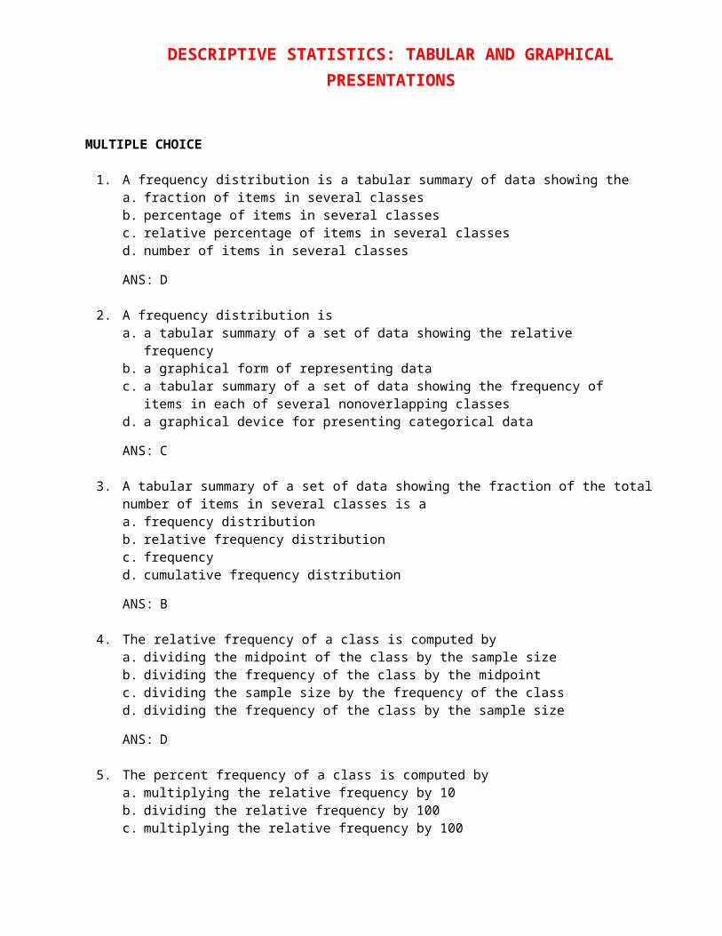
1. A frequency distribution is a tabular summary of data showing thea. fraction of items in several classesb. percentage of items in several classesc. relative percentage of items in several classesd. number of items in several classes

ANS: D

2. A frequency distribution isa. a tabular summary of a set of data showing the relative frequencyb. a graphical form of representing datac. a tabular summary of a set of data showing the frequency of items in each of several

nonoverlapping classesd. a graphical device for presenting categorical data

ANS: C

3. A tabular summary of a set of data showing the fraction of the total number of items in several classes is aa. frequency distributionb. relative frequency distributionc. frequencyd. cumulative frequency distribution

ANS: B

4. The relative frequency of a class is computed bya. dividing the midpoint of the class by the sample sizeb. dividing the frequency of the class by the midpointc. dividing the sample size by the frequency of the classd. dividing the frequency of the class by the sample size

ANS: D

5. The percent frequency of a class is computed bya. multiplying the relative frequency by 10b. dividing the relative frequency by 100c. multiplying the relative frequency by 100d. adding 100 to the relative frequency

ANS: C

6. The sum of frequencies for all classes will always equala. 1b. the number of elements in a data setc. the number of classesd. a value between 0 and 1

ANS: B

7. Fifteen percent of the students in a school of Business Administration are majoring in Economics, 20% in Finance, 35% in Management, and 30% in Accounting. The graphical device(s) which can be used to present these data is (are)a. a line chartb. only a bar chartc. only a pie chartd. both a bar chart and a pie chart

ANS: D

8. A researcher is gathering data from four geographical areas designated: South = 1; North = 2; East = 3; West = 4. The designated geographical regions representa. categorical datab. quantitative datac. label datad. either quantitative or categorical data

ANS: A

9. Categorical data can be graphically represented by using a(n)a. histogramb. frequency polygonc. ogived. bar chart

ANS: D

10. A cumulative relative frequency distribution showsa. the proportion of data items with values less than or equal to the upper limit of each classb. the proportion of data items with values less than or equal to the lower limit of each classc. the percentage of data items with values less than or equal to the upper limit of each classd. the percentage of data items with values less than or equal to the lower limit of each class

ANS: A

11. If several frequency distributions are constructed from the same data set, the distribution with the widest class width will have thea. fewest classesb. most classesc. same number of classes as the other distributions since all are constructed from the same

data

ANS: A

12. The sum of the relative frequencies for all classes will always equala. the sample sizeb. the number of classesc. One

d. any value larger than one

ANS: C

13. The sum of the percent frequencies for all classes will always equala. oneb. the number of classes

c. the number of items in the studyd. 100

ANS: D

14. The most common graphical presentation of quantitative data is aa. histogramb. bar chartc. relative frequencyd. pie chart

ANS: A

15. The total number of data items with a value less than the upper limit for the class is given by thea. frequency distributionb. relative frequency distributionc. cumulative frequency distributiond. cumulative relative frequency distribution

ANS: C

16. The relative frequency of a class is computed bya. dividing the cumulative frequency of the class by nb. dividing n by cumulative frequency of the classc. dividing the frequency of the class by nd. dividing the frequency of the class by the number of classes

ANS: C

17. In constructing a frequency distribution, the approximate class width is computed asa. (largest data value - smallest data value)/number of classesb. (largest data value - smallest data value)/sample sizec. (smallest data value - largest data value)/sample sized. largest data value/number of classes

ANS: A

18. In constructing a frequency distribution, as the number of classes are decreased, the class widtha. decreasesb. remains unchangedc. increasesd. can increase or decrease depending on the data values

ANS: C

19. The difference between the lower class limits of adjacent classes provides thea. number of classesb. class limitsc. class midpointd. class width

ANS: D

20. In a cumulative frequency distribution, the last class will always have a cumulative frequency equal toa. one

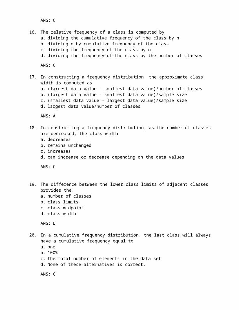
b. 100%c. the total number of elements in the data setd. None of these alternatives is correct.

ANS: C

21. In a cumulative relative frequency distribution, the last class will have a cumulative relative frequency equal toa. oneb. zeroc. the total number of elements in the data setd. None of these alternatives is correct.

ANS: A

22. In a cumulative percent frequency distribution, the last class will have a cumulative percent frequency equal toa. oneb. 100c. the total number of elements in the data setd. None of these alternatives is correct.

ANS: B

23. Data that provide labels or names for categories of like items are known asa. categorical datab. quantitative datac. label datad. category data

ANS: A

24. A tabular method that can be used to summarize the data on two variables simultaneously is calleda. simultaneous equationsb. crosstabulationc. a histogramd. an ogive

ANS: B

25. A graphical presentation of the relationship between two variables isa. an ogiveb. a histogramc. either an ogive or a histogram, depending on the type of datad. a scatter diagram

ANS: D

26. A histogram is said to be skewed to the left if it has aa. longer tail to the rightb. shorter tail to the rightc. shorter tail to the leftd. longer tail to the left

ANS: D

27. When a histogram has a longer tail to the right, it is said to bea. symmetricalb. skewed to the leftc. skewed to the rightd. none of these alternatives is correct

ANS: C

28. In a scatter diagram, a line that provides an approximation of the relationship between the variables is known asa. approximation lineb. trend linec. line of zero interceptd. line of zero slope

ANS: B

29. A histogram isa. a graphical presentation of a frequency or relative frequency distributionb. a graphical method of presenting a cumulative frequency or a cumulative relative

frequency distributionc. the history of data elementsd. the same as a pie chart

ANS: A

30. A situation in which conclusions based upon aggregated crosstabulation are different from unaggregated crosstabulation is known asa. wrong crosstabulationb. Simpson's rulec. Simpson's paradoxd. aggregated crosstabulation

ANS: C

Exhibit 2-1The numbers of hours worked (per week) by 400 statistics students are shown below.

Number of hours Frequency  0 -   9   2010 - 19   8020 - 29 20030 - 39 100

31. Refer to Exhibit 2-1. The class width for this distributiona. is 9b. is 10c. is 39, which is: the largest value minus the smallest value or 39 - 0 = 39d. varies from class to class

ANS: B

32. Refer to Exhibit 2-1. The number of students working 19 hours or less

a. is 80b. is 100c. is 180d. is 300

ANS: B

33. Refer to Exhibit 2-1. The relative frequency of students working 9 hours or lessa. is 20b. is 100c. is 0.95d. 0.05

ANS: D

34. Refer to Exhibit 2-1. The percentage of students working 19 hours or less isa. 20%b. 25%c. 75%d. 80%

ANS: B

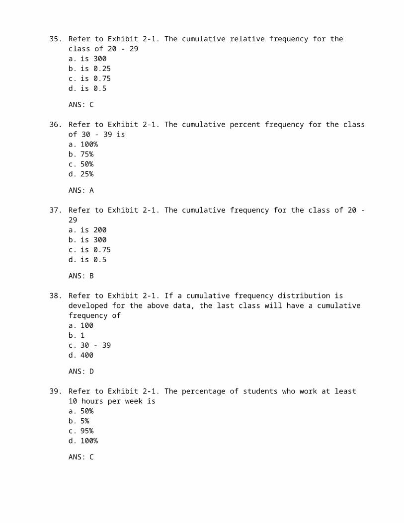
35. Refer to Exhibit 2-1. The cumulative relative frequency for the class of 20 - 29a. is 300b. is 0.25c. is 0.75d. is 0.5

ANS: C

36. Refer to Exhibit 2-1. The cumulative percent frequency for the class of 30 - 39 isa. 100%b. 75%c. 50%d. 25%

ANS: A

37. Refer to Exhibit 2-1. The cumulative frequency for the class of 20 - 29a. is 200b. is 300c. is 0.75d. is 0.5

ANS: B

38. Refer to Exhibit 2-1. If a cumulative frequency distribution is developed for the above data, the last class will have a cumulative frequency ofa. 100b. 1c. 30 - 39d. 400

ANS: D

39. Refer to Exhibit 2-1. The percentage of students who work at least 10 hours per week isa. 50%b. 5%c. 95%d. 100%

ANS: C

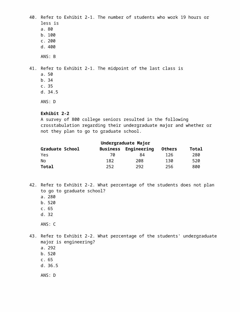
40. Refer to Exhibit 2-1. The number of students who work 19 hours or less isa. 80b. 100c. 200d. 400

ANS: B

41. Refer to Exhibit 2-1. The midpoint of the last class isa. 50b. 34c. 35d. 34.5

ANS: D

Exhibit 2-2A survey of 800 college seniors resulted in the following crosstabulation regarding their undergraduate major and whether or not they plan to go to graduate school.

Undergraduate MajorGraduate School Business Engineering Others TotalYes   70   84 126 280No 182 208 130 520Total 252 292 256 800

42. Refer to Exhibit 2-2. What percentage of the students does not plan to go to graduate school?a. 280b. 520c. 65d. 32

ANS: C

43. Refer to Exhibit 2-2. What percentage of the students' undergraduate major is engineering?a. 292b. 520c. 65d. 36.5

ANS: D

44. Refer to Exhibit 2-2. Of those students who are majoring in business, what percentage plans to go to graduate school?a. 27.78b. 8.75

c. 70d. 72.22

ANS: A

45. Refer to Exhibit 2-2. Among the students who plan to go to graduate school, what percentage indicated "Other" majors?a. 15.75b. 45c. 54d. 35

ANS: B

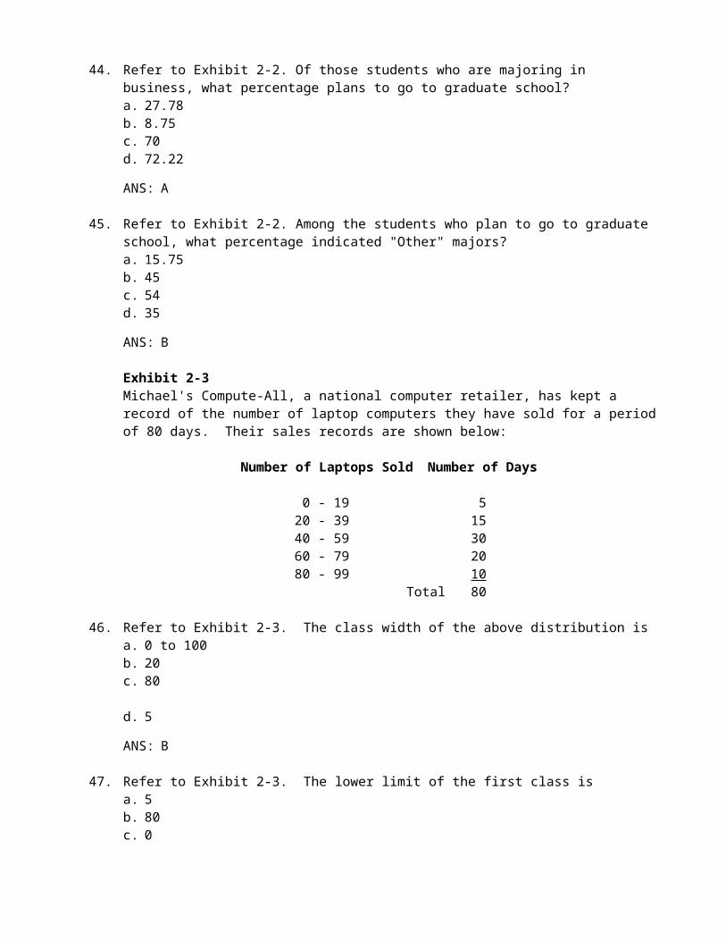
Exhibit 2-3Michael's Compute-All, a national computer retailer, has kept a record of the number of laptop computers they have sold for a period of 80 days. Their sales records are shown below:

Number of Laptops Sold Number of Days

0 - 19 520 - 39 1540 - 59 3060 - 79 2080 - 99 10

Total 80

46. Refer to Exhibit 2-3. The class width of the above distribution isa. 0 to 100b. 20c. 80

d. 5

ANS: B

47. Refer to Exhibit 2-3. The lower limit of the first class isa. 5b. 80c. 0d. 20

ANS: C

48. Refer to Exhibit 2-3. If one develops a cumulative frequency distribution for the above data, the last class will have a frequency ofa. 10b. 100c. 0 to 100d. 80

ANS: D

49. Refer to Exhibit 2-3. The percentage of days in which the company sold at least 40 laptops isa. 37.5%

b. 62.5%c. 90.0%d. 75.0%

ANS: D

50. Refer to Exhibit 2-3. The number of days in which the company sold less than 60 laptops isa. 20b. 30c. 50d. 60

ANS: C

PROBLEM

1. Thirty students in the School of Business were asked what their majors were. The following represents their responses (M = Management; A = Accounting; E = Economics; O = Others).

A M M A M M E M O AE E M A O E M A M AM A O A M E E M A M

a. Construct a frequency distribution and a bar chart.b. Construct a relative frequency distribution and a pie chart.

ANS:

(a) (b)

Major FrequencyRelative

FrequencyM 12 0.4A   9 0.3E   6 0.2O     3 0.1Total 30 1.0

2. Twenty employees of the Ahmadi Corporation were asked if they liked or disliked the new district manager. Below you are given their responses. Let L represent liked and D represent disliked.

L L D L DD D L L DD L D D LD D L D L

a. Construct a frequency distribution and a bar chart.b. Construct a relative frequency distribution and a pie chart.

ANS:a and b

Preferences FrequencyRelative

FrequencyL   9 0.45D 11 0.55Total 20 1.00

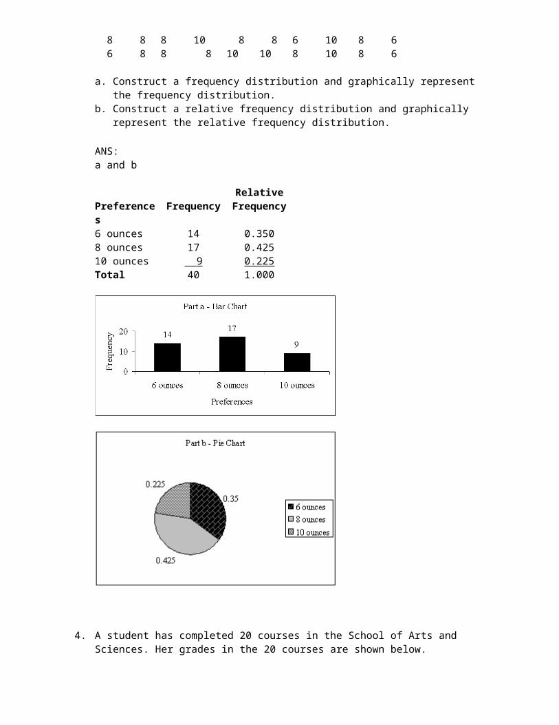
3. Forty shoppers were asked if they preferred the weight of a can of soup to be 6 ounces, 8 ounces, or 10 ounces. Below you are given their responses.

  6   6 6 10   8   8 8 10 6 610 10 8   8   6   6 6   8 6 6  8   8 8 10   8   8 6 10 8 6  6   8 8   8 10 10 8 10 8 6

a. Construct a frequency distribution and graphically represent the frequency distribution.b. Construct a relative frequency distribution and graphically represent the relative frequency

distribution.

ANS:a and b

Preferences FrequencyRelative

Frequency6 ounces 14 0.3508 ounces 17 0.42510 ounces     9 0.225Total 40 1.000

4. A student has completed 20 courses in the School of Arts and Sciences. Her grades in the 20 courses are shown below.

A B A B CC C B B BB A B B BC B C B A

a. Develop a frequency distribution and a bar chart for her grades.b. Develop a relative frequency distribution for her grades and construct a pie chart.

ANS:a and b

Grade FrequencyRelative

FrequencyA   4 0.20B 11 0.55C     5 0.25Total 20 1.00

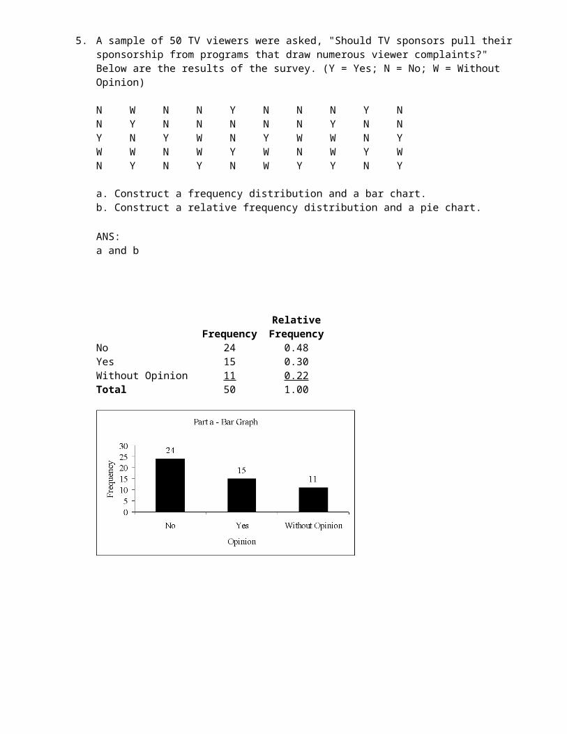
5. A sample of 50 TV viewers were asked, "Should TV sponsors pull their sponsorship from programs that draw numerous viewer complaints?" Below are the results of the survey. (Y = Yes; N = No; W = Without Opinion)

N W N N Y N N N Y NN Y N N N N N Y N NY N Y W N Y W W N YW W N W Y W N W Y WN Y N Y N W Y Y N Y

a. Construct a frequency distribution and a bar chart.b. Construct a relative frequency distribution and a pie chart.

ANS:a and b

FrequencyRelative

FrequencyNo 24 0.48Yes 15 0.30Without Opinion 11 0.22Total 50 1.00

6. Below you are given the examination scores of 20 students.

52 99 92 86 8463 72 76 95 8892 58 65 79 8090 75 74 56 99

a. Construct a frequency distribution for this data. Let the first class be 50 - 59 and draw a histogram.

b. Construct a cumulative frequency distribution.c. Construct a relative frequency distribution.d. Construct a cumulative relative frequency distribution.

ANS:

a. b. c. d.Cumulative

Cumulative Relative RelativeScore Frequency Frequency Frequency Frequency50 - 59 3   3 0.15 0.1560 - 69 2   5 0.10 0.2570 - 79 5 10 0.25 0.5080 - 89 4 14 0.20 0.7090 - 99 6 20 0.30 1.00Total 20 1.00

7. The frequency distribution below was constructed from data collected from a group of 25 students.

Height(in Inches) Frequency

58 - 63 364 - 69 570 - 75 276 - 81 6

82 - 87 488 - 93 394 - 99 2

a. Construct a relative frequency distribution.b. Construct a cumulative frequency distribution.c. Construct a cumulative relative frequency distribution.

ANS:

a. b. c.Cumulative

Height Relative Cumulative Relative(In Inches) Frequency Frequency Frequency Frequency

58 - 63 3 0.12 3 0.1264 - 69 5 0.20 8 0.3270 - 75 2 0.08 10 0.4076 - 81 6 0.24 16 0.6482 - 87 4 0.16 20 0.8088 - 93 3 0.12 23 0.9294 - 99 2 0.08 25 1.00

1.00

8. The frequency distribution below was constructed from data collected on the quarts of soft drinks consumed per week by 20 students.

Quarts ofSoft Drink Frequency

0 - 3 4 4 - 7 5 8 - 11 612 - 15 316 - 19 2

a. Construct a relative frequency distribution.b. Construct a cumulative frequency distribution.c. Construct a cumulative relative frequency distribution.

ANS:

a. b. c.Cumulative

Quarts of Relative Cumulative RelativeSoft Drinks Frequency Frequency Frequency Frequency

  0 -   4 4 0.20   4 0.20  4 -   8 5 0.25   9 0.45  8 - 12 6 0.30 15 0.7512 - 16 3 0.15 18 0.9016 - 20 2 0.10 20 1.00

Total 20 1.00

9. The grades of 10 students on their first management test are shown below.

94 61 96 66 9268 75 85 84 78

a. Construct a frequency distribution. Let the first class be 60 - 69.b. Construct a cumulative frequency distribution.c. Construct a relative frequency distribution.

ANS:

a. b. c.Cumulative Relative

Class Frequency Frequency Frequency60 - 69 3   3 0.370 - 79 2   5 0.280 - 89 2   7 0.290 - 99 3 10 0.3Total 10 1.0

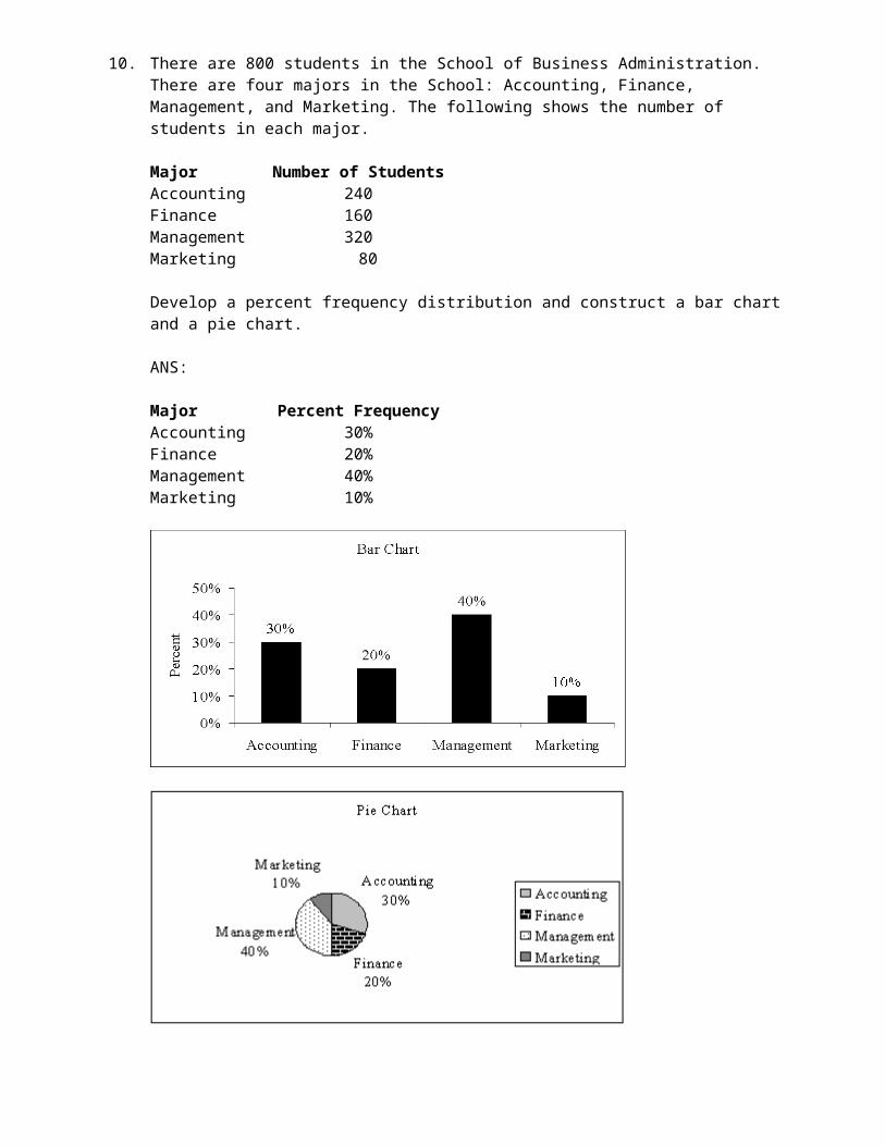
10. There are 800 students in the School of Business Administration. There are four majors in the School: Accounting, Finance, Management, and Marketing. The following shows the number of students in each major.

Major Number of StudentsAccounting 240Finance 160Management 320Marketing   80

Develop a percent frequency distribution and construct a bar chart and a pie chart.

ANS:

Major Percent FrequencyAccounting 30%Finance 20%Management 40%Marketing 10%

11. You are given the following data on the ages of employees at a company. Construct a stem-and-leaf display.

26 32 28 45 5852 44 36 42 2741 53 55 48 3242 44 40 36 37

ANS:

2 | 6 7 83 | 2 2 6 6 74 | 0 1 2 2 4 4 5 85 | 2 3 5 8

12. Construct a stem-and-leaf display for the following data.

12 52 51 37 47 40 38 26 57 3149 43 45 19 36 32 44 48 22 18

ANS:

1 | 2 8 92 | 2 63 | 1 2 6 7 84 | 0 3 4 5 7 8 95 | 1 2 7

13. The SAT scores of a sample of business school students and their genders are shown below.

SAT ScoresGender Less than 20 20 up to 25 25 and more TotalFemale 24 168 48 240Male 40   96 24 160Total 64 264 72 400

a. How many students scored less than 20?b. How many students were female?c. Of the male students, how many scored 25 or more?d. Compute row percentages and comment on any relationship that may exist between SAT

scores and gender of the individuals.e. Compute column percentages.

ANS:

a. 64b. 240c. 24

d. SAT ScoresGender Less than 20 20 up to 25 25 and more TotalFemale 10% 70% 20% 100%Male 25% 60% 15% 100%

From the above percentages it can be noted that the largest percentages of both genders' SAT scores are in the 20 to 25 range. However, 70% of females and only 60% of males have SAT scores in this range. Also it can be noted that 10% of females' SAT scores are under 20, whereas, 25% of males' SAT scores fall in this category.

e. SAT ScoresGender Less than 20 20 up to 25 25 and moreFemale 37.5% 63.6% 66.7%Male 62.5% 36.4% 33.3%Total 100% 100% 100%

14. For the following observations, plot a scatter diagram and indicate what kind of relationship (if any) exist between x and y.

x y2 76 193 95 174 11

ANS:A positive relationship between x and y appears to exist.

15. For the following observations, plot a scatter diagram and indicate what kind of relationship (if any) exist between x and y.

x y8 45 53 92 121 14

ANS:A negative relationship between x and y appears to exist.

16. Five hundred recent graduates indicated their majors as follows.

Major Frequency

Accounting 60Finance 100Economics 40Management 120Marketing 80Engineering 60Computer Science 40Total 500

a. Construct a relative frequency distribution.b. Construct a percent frequency distribution.

ANS:

a. b.Relative Percent

Major Frequency Frequency Frequency

Accounting 60 0.12 12Finance 100 0.20 20Economics 40 0.08 8Management 120 0.24 24Marketing 80 0.16 16Engineering 60 0.12 12Computer Science 40 0.08 8Total 500 1.00 100

17. A sample of the ages of 10 employees of a company is shown below.

20 30 40 30 5030 20 30 20 40

Construct a dot plot for the above data.

ANS:•

• •• • •• • • •

10 20 30 40 50 60

18. The following data set shows the number of hours of sick leave that some of the employees of Bastien's, Inc. have taken during the first quarter of the year (rounded to the nearest hour).

19 22 27 24 28 1223 47 11 55 25 4236 25 34 16 45 4912 20 28 29 21 1059 39 48 32 40 31

a. Develop a frequency distribution for the above data. (Let the width of your classes be 10 units and start your first class as 10 - 19.)

b. Develop a relative frequency distribution and a percent frequency distribution for the data.c. Develop a cumulative frequency distribution.d. How many employees have taken less than 40 hours of sick leave?

ANS:

a. b. b. c.Hours of Relative Percent Cum.

Sick Leave Taken Freq. Freq. Freq. Freq.10 - 19 6 0.20 20 620 - 29 11 0.37 37 1730 - 39 5 0.16 16 2240 - 49 6 0.20 20 2850 - 59 2 0.07 7 30

d. 22

19. The sales record of a real estate company for the month of May shows the following house prices (rounded to the nearest $1,000). Values are in thousands of dollars.

105 55 45 85 7530 60 75 79 95

a. Develop a frequency distribution and a percent frequency distribution for the house prices. (Use 5 classes and have your first class be 20 - 39.)

b. Develop a cumulative frequency and a cumulative percent frequency distribution for the above data.

c. What percentage of the houses sold at a price below $80,000?

ANS:

a. a. b. b.Cum.

Sales Price Percent Cum. Percent(In Thousands of Dollars) Freq. Freq. Freq. Freq.

20 - 39 1 10 1 1040 - 59 2 20 3 3060 - 79 4 40 7 70

80 - 99 2 20 9 90100 - 119 1 10 10 100

c. 70%

20. The test scores of 14 individuals on their first statistics examination are shown below.

95 87 52 43 77 84 7875 63 92 81 83 91 88

Construct a stem-and-leaf display for these data.

ANS:4 35 26 37 5 7 88 1 3 4 7 89 1 2 5

21. A survey of 400 college seniors resulted in the following crosstabulation regarding their undergraduate major and whether or not they plan to go to graduate school.

Undergraduate Major

Graduate School Business Engineering Others Total

Yes 35 42 63 140

No 91 104 65 260

Total 126 146 128 400

a. Are a majority of the seniors in the survey planning to attend graduate school?b. Which discipline constitutes the majority of the individuals in the survey?c. Compute row percentages and comment on the relationship between the students'

undergraduate major and their intention of attending graduate school.d. Compute the column percentages and comment on the relationship between the students'

intention of going to graduate school and their undergraduate major.

ANS:a. No, majority (260) will not attend graduate schoolb. Majority (146) are engineering majorsc.

Undergraduate Major

Graduate School Business Engineering Others Total

Yes 25% 30% 45% 100%

No 35% 40% 25% 100% Majority who plan to go to graduate school are from "Other" majors. Majority of those who will not

go to graduate school are engineering majors.

d.Undergraduate Major

Graduate School Business Engineering Others

Yes 27.8% 28.8% 49.2%

No 72.2% 71.2% 50.8%

Total 100% 100% 100%

Approximately the same percentages of Business and engineering majors plan to attend graduate school (27.8% and 28.8% respectively). Of the "Other" majors approximately half (49.2%) plan to go to graduate school.