Video Stabilization using Robust Feature Trajectories

Ken-Yi Lee Yung-Yu Chuang Bing-Yu Chen Ming OuhyoungNational Taiwan University

{kez|cyy|robin|ming}@cmlab.csie.ntu.edu.tw

Abstract

This paper proposes a new approach for video stabi-lization. Most existing video stabilization methods adopta framework of three steps, motion estimation, motion com-pensation and image composition. Camera motion is oftenestimated based on pairwise registration between frames.Thus, these methods often assume static scenes or distantbackgrounds. Furthermore, for scenes with moving objects,robust methods are required for finding the dominant mo-tion. Such assumptions and judgements could lead to errorsin motion parameters. Errors are compounded by motioncompensation which smoothes motion parameters. This pa-per proposes a method to directly stabilize a video withoutexplicitly estimating camera motion, thus assuming neithermotion models nor dominant motion. The method first ex-tracts robust feature trajectories from the input video. Op-timization is then performed to find a set of transformationsto smooth out these trajectories and stabilize the video. Inaddition, the optimization also considers quality of the sta-bilized video and selects a video with not only smooth cam-era motion but also less unfilled area after stabilization. Ex-periments show that our method can deal with complicatedvideos containing near, large and multiple moving objects.

1. IntroductionHand-held video capturing devices become more and

more accessible today because of lowering prices and re-

ducing sizes. While people enjoy the luxury of capturing

interesting moments with more ease, it also leads to a great

amount of videos captured casually by amateurs without

carefully planning [7]. Such a casual video often exhibits

annoying jitter due to shaky motion of an unsteady hand-

held camera or a vehicle-mounted camera. Therefore, to

enhance user’s experiences in watching casual videos, videostabilization, removing unwanted video perturbations due

to unstable camera motions, plays an important role.

A video can be stabilized during recording or with

an offline post-processing. Nowadays, many cameras are

equipped with hardware stabilizers. Expensive high-end

cameras usually have sophisticated sensors and lens sys-

tems to remove camera shake during recording. Cheaper

cameras may use sensors to estimate camera motion and

built-in firmware to properly crop the acquired images for

compensating the jittered motion [10]. Such online solu-

tions are often not sufficient for dealing with sequences with

complicated motions. Therefore, even using a camera with

an online stabilizer, unwanted camera jerks still happen fre-

quently in videos taken by non-professional users. Thus,

offline video stabilization algorithms are still required for

making these videos steady.

Most video stabilization methods follow a three-step

framework consisting of three steps: motion estimation, mo-tion compensation (also called motion smoothing or mo-tion filtering) and image composition [15]. Motion estima-

tion estimates the motion between frames. The estimated

motion parameters are forwarded to motion compensation,

which damps camera motion by removing high-frequency

fluctuations and computes the global transformation neces-

sary to stabilize the current frame. Finally, image compo-

sition warps the current frame according to that transfor-

mation and generates the stabilized sequence. Optionally,

image composition could include inpainting and deblurring

to further improve the quality of the stabilized video. Most

previous video stabilization methods focused on improving

components of this framework. For example, many algo-

rithms have been proposed for improving camera compen-

sation by better smoothing out camera motion or recovering

the intentional camera motion [1, 6, 11, 16, 20]. Some fo-

cused on improving image composition by motion inpaint-

ing and deblurring [14]. However, this three-step frame-

work was kept intact in most video stabilization algorithms.

Most previous video stabilization methods need to make

assumptions on motion models for motion estimation. Flex-

ible motion models, such as optical flow, could be used but

they bring more challenges on smoothing motion parame-

ters for motion compensation. Therefore, simpler models

such as planar homography are more popular. Although

these models can be fitted more robustly, they have many re-

strictions on scene and motion properties. For scenes with

great depth variations or multiple moving objects, robust

1397 2009 IEEE 12th International Conference on Computer Vision (ICCV) 978-1-4244-4419-9/09/$25.00 ©2009 IEEE

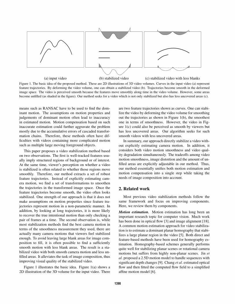
(a) input video (b) stabilized video (c) stabilized video with less blanks

Figure 1. The basic idea of the proposed method. These are 2D illustrations of 3D video volumes. Curves in the input video (a) represent

feature trajectories. By deforming the video volume, one can obtain a stabilized video (b). Trajectories become smooth in the deformed

image space. The video is perceived smooth because the features move smoothly along time in the video volume. However, some areas

become unfilled (as shaded in the figure). Our method seeks for a video which is not only stabilized but also has less uncovered areas (c).

means such as RANSAC have to be used to find the dom-

inant motion. The assumptions on motion properties and

judgements of dominant motion often lead to inaccuracy

in estimated motion. Motion compensation based on such

inaccurate estimation could further aggravate the problem

mostly due to the accumulative errors of cascaded transfor-

mation chains. Therefore, these methods often have dif-

ficulties with videos containing more complicated motion

such as multiple large moving foreground objects.

This paper proposes a video stabilization method based

on two observations. The first is well-tracked features usu-

ally imply structured regions of background or of interest.

At the same time, viewer’s perception on whether a video

is stabilized is often related to whether those regions move

smoothly. Therefore, our method extracts a set of robust

feature trajectories. Instead of explicitly estimating cam-

era motion, we find a set of transformations to smoothen

the trajectories in the transformed image space. Once the

feature trajectories become smooth, the video often looks

stabilized. One strength of our approach is that it does not

make assumptions on motion properties since feature tra-

jectories represent motion in a non-parametric manner. In

addition, by looking at long trajectories, it is more likely

to recover the true intentional motion than only checking a

pair of frames at a time. The second observation is, while

most stabilization methods find the best camera motion in

terms of the smoothness measurement they used, there are

actually many camera motions that viewers feel stabilized

enough. To avoid leaving large blank areas for image com-

position to fill, it is often possible to find a sufficiently

smooth motion with less blank areas. The result is a sta-

bilized video with both smooth camera motion and less un-

filled areas. It alleviates the task of image composition, thus

improving visual quality of the stabilized video.

Figure 1 illustrates the basic idea. Figure 1(a) shows a

2D illustration of the 3D volume for the input video. There

are two feature trajectories shown as curves. One can stabi-

lize the video by deforming the video volume for smoothing

out the trajectories as shown in Figure 1(b), the smoothest

one in terms of smoothness. However, the video in Fig-

ure 1(c) could also be perceived as smooth by viewers but

has less uncovered areas. Our algorithm seeks for such

smooth videos with less uncovered areas.

In summary, our approach directly stabilize a video with-

out explicitly estimating camera motion. In addition, it

considers both video motion smoothness and video qual-

ity degradation simultaneously. The tradeoffs among video

motion smoothness, image distortion and the amount of un-

filled areas are explicitly adjustable in our method. Thus,

our method essentially unifies both motion estimation and

motion compensation into a single step while taking the

needs of image composition into account.

2. Related work

Most previous video stabilization methods follow the

same framework and focus on improving components.

Here, we review them by components.

Motion estimation. Motion estimation has long been an

important research topic for computer vision. Much work

has been done in optical flow [3] and image alignment [18].

A common motion estimation approach for video stabiliza-

tion is to estimate a dominant planar homography that stabi-

lizes a large planar region in the video [5]. Both direct and

feature-based methods have been used for homography es-

timation. Homography-based schemes generally performs

quite well for stabilizing planar scenes or rotational camera

motions but suffers from highly non-planar scenes. Jin etal. proposed a 2.5D motion model to handle sequences with

significant depth changes [9]. Chang et al. estimated optical

flow and then fitted the computed flow field to a simplified

affine motion model [6].

1398

Motion compensation. The goal of motion compensation is

to remove high-frequency jitters from the estimated camera

motion. It is the component that most video stabilization al-

gorithms attempt to improve and many methods have been

proposed, such as motion vector integration [1], particle fil-

ter [20], variational method [16], regularization [6], Kalman

filter [11] and local parabolic fitting [8].

Image composition. Some focus on improving video qual-

ity degradation caused by stabilization. Hu et al. used dy-

namic programming to reduce the visual artifacts in the

boundary of defined areas and mosaics [8]. Matsushita etal. used motion inpainting to fill in the unfilled area for

full-frame stabilization and deblurring for further improv-

ing video quality [14]. Gleicher et al. compensated esti-

mated camera motions and considered video quality loss at

the same time [7].

3. Robust feature trajectoriesExtracting robust feature trajectories from a video is a

crucial step for our method. It is certainly possible to con-

catenate frame-by-frame feature matches to obtain long-

range trajectories. However, feature matching is best suited

to successive pairs of frames, not to long sequences. A false

match often severely messes up the whole feature trajec-

tory. Thus, trajectories must be concatenated and pruned

carefully to avoid false matches’ terrible impacts.

Our robust feature trajectory extraction algorithm incor-

porates spatial motion consistency to reduce false matches

and temporal motion similarity of trajectories for long-

range tracking. It is a marriage of particle video [17] and

SIFT flow [12]. The overall flow of our algorithm is similar

to particle video, a framework for estimating dense particle-

level long-range motion of a video based on optical flow.

For efficiency and robustness, we adapt this framework but

using reliable feature tracking. On the other hand, although

the workflow is similar to particle video, our optimization

is more similar to SIFT flow as it is formulated as a discrete

optimization problem.

Our algorithm retrieves feature trajectories by making a

forward sweep across the video. Here, a trajectory ξj is a set

of 2D points {ptj |ts ≤ t≤ te} across time defined between

its start time ts and end time te. Assume that, after finishing

frame t, we have a set of live trajectories Γ = {ξj}. For the

next frame t+1, the following four steps are performed to

reliably extend the live trajectories to the next frame.

Addition. We use feature detection to generate feature

points {f t+1i } for frame t+1. Our current implementation

uses SIFT [13] for its accuracy and robustness in different

lighting and blurring conditions.

Linking. For incorporating motion consistency to spatially

neighboring features, we need to assign neighbor relation-

ships to features. Delaunay triangulation is applied on the

detected feature points. If any pair of feature points share

an edge, they are considered neighbors. Such neighborhood

information propagates with the trajectories through the en-

tire video until the trajectories are pruned. In other words,

two trajectories are neighbors as long as they share an edge

in some frame.

Propagation by optimization. Feature points are propa-

gated by using feature matching. If there is a similar fea-

ture in the next frame, the feature point will be propagated.

However, there might be many similar features in the next

frame, an optimization step helps choose the best match to

propagate by considering feature similarity and neighbors’

motion consistency. If temporal movement of two trajecto-

ries exhibits a similar pattern in the past, it is more likely

that they will move similarly at the current frame as they

are often on the same surface patch. Thus, the algorithm

prefers to move two trajectories with high temporal motion

similarity in a similar manner.

Let Φt be a match assignment for frame t, which assigns

feature points at frame t+1 to trajectories at time t. For

example, Φt(i) = j means to extend the i-th trajectory ξi

to the j-th feature point f t+1j at frame t+1. In other words,

it means to assign f t+1j as pt+1

i , the point at frame t+1for trajectory ξi. Note that Φt is injective as it describes

correspondences. It also means that Φt(i) could be null

if there are more trajectories than detected features. With

such an assignment, the motion flow uti for the i-th trajec-

tory at frame t for this assignment Φt can then be define as

uti(Φ

t) = f t+1Φt(i)−pt

i since f t+1Φt(i) is frame t+1’s correspon-

dence for pti.

Our goal is to find the optimal assignment which assigns

good matches but also maintains good motion similarity

for neighboring features by minimizing the following cost

function:

E(Φt) =∑

i

‖ s(pti)− s(f t+1

Φt(i)) ‖2

+λt

∑(i,j)∈N

wij ‖ uti(Φ

t)− utj(Φ

t) ‖2, (1)

where s(p) is the SIFT descriptor of point p, N is the set

of all neighbor pairs and λt controls the tradeoff between

two terms. The first term penalizes feature mismatches and

the second term punishes motion inconsistency of neighbor-

ing features. Similar to particle video, link weights wij is

measured by a weighted sum of past motion similarity as

vti =pt+1

i − pti,

Dij =1|τ |

∑t∈τ

‖ vti − vt

j ‖2,

wij =G(√

Dij ;σd),

where τ is a set of previous frames and G(·;σ) is a zero-

mean Gaussian with the standard deviation σ. Dij measures

1399

the motion similarity between trajectory i and trajectory jby averaging their flow differences for a number of frames.

Similar to SIFT flow, the problem of robust feature cor-

respondence is formulated as a discrete optimization prob-

lem as shown in Equation 1. We use a greedy best-match

approach to speed up the optimization. Although there is

no guarantee for global optimum, it works pretty well in

practice. In addition, even if the greedy approach may dis-

card some possible alternatives and lead to mismatches, this

problem can be corrected in the next step.

Pruning. After propagation, all trajectories at the current

frame are stretched to correspondent positions in the next

frame. If there are more trajectories than detected features,

unassigned trajectories are terminated, removed from the

live trajectory set Γ and added to a retired trajectory set Π.

Similarly, if there are more features than trajectories, the

unmapped features will start new trajectories and are added

to Γ for the next frame. In addition, extended trajectories

with low feature similarity and/or bad neighbor consistency

will also be pruned and added to the retired trajectory set Π.

The cost of trajectory i is defined as

‖ s(pti)− s(f t+1

Φt(i)) ‖2 +λt

∑j∈N(i)

wij ‖ uti(Φ

t)− utj(Φ

t) ‖2

and trajectories with costs higher than a threshold are

pruned. Remaining matches are used to extend the trajec-

tories by letting ξi = ξi ∪ {f t+1Φt(i)}, i.e., assigning f t+1

Φt(i) to

pt+1i . These trajectories are kept in Γ for the next frame.

By repeating the above four steps frame by frame

through the entire video, we can retrieve a set of robust fea-

ture trajectories Π from the input video. It is worthy noted

that, since neighbor information is considered during track-

ing, features tend to move as a patch but not as single points.

This is helpful for our stabilization.

4. Video stabilization by optimization

Smoothness of a curve is often measured by the sum

of squared values of the second derivative (acceleration).

Therefore, in a perfectly stabilized video, features should

move in a constant velocity in image space. Thus, instead

of estimating and compensating real camera motions, we

estimate a set of geometric transformations so that features

move along their trajectories approximately in a constant

velocity in the image space after being transformed.

Another factor we take into account is image quality

degradation after transformation. When a frame is warped

by a transformation, the image quality may be degraded.

This degradation comes from two sources. First, after trans-

formation, some areas become uncovered in the warped

frame. Second, a transformation with a scale factor larger

than one stretches the image. Although these problems

could be alleviated by inpainting and super-resolution al-

gorithms, these algorithms are not perfect and artifacts may

still remain in the stabilized video. Our solution is to con-

sider image degradation during the search of transforma-

tions for smoothing transformed trajectories.

In the following, we first present how trajectories are

weighted for robustness (Section 4.1), then explain the con-

struction of the objective function (Section 4.2), and finally

describe how to find the optimal solution (Section 4.3).

4.1. Trajectory weights

Section 3 retrieves a set of robust trajectories Π = {ξi}from the input video. Although there are good trajectories

that do relate to real camera shakes, some include wrong

matches and some belong to self-moving objects unrelated

to camera motion. Therefore, not every trajectory has equal

importance and we need a mechanism for emphasizing im-

pacts of good trajectories. When a trajectory comes from

a region of background or of interest, it should have higher

importance. In general, longer trajectories are more impor-

tant as they often represent objects of interest in motion or

static background due to the moving camera. Both cases are

useful for stabilizing a video. On the other hand, fast mo-

tions often lead to short trajectories as the feature matching

is less reliable. As fast foreground motion is often not re-

lated to camera shakes, we would like to depreciate short

trajectories when stabilizing cameras. Therefore, we mea-

sure the importance of a trajectory by its temporal persis-

tence and give higher weights to longer trajectories. In addi-

tion, the weight should be a function of time as well. That is,

a trajectory could contribute differently for different frames.

A trajectory should have more impact to a frame if the frame

is on the middle of the trajectory. On the other hand, an

emerging or vanishing trajectory should have less impact to

the frame. Thus, we used a triangle function to give higher

weights toward the middle of the trajectory. Let’s denote the

contribution of the i-th trajectory ξi to frame t as wti which

is proportional to lti = min(t − ts(ξi), te(ξi) − t), where

ts(ξi) and te(ξi) denote the start time and end time of ξi.

Finally, a couple of normalization steps are required.

A spatial normalization is used to avoid dominant spots if

many trajectories gather around some spots (Equation 2).

This normalization has the effects to consider trajectories

more evenly in space. A temporal normalization is applied

to normalize trajectory weights of a frame by the number of

trajectories going through the frame (Equation 3).

w̃ti =

lti∑j∈Π(t) G(|pt

j − pti|;σs)

, (spatial) (2)

wti =

w̃ti∑

j∈Π(t) w̃tj

, (normalization) (3)

where Π(t) is the set of trajectories going through frame t.

1400

Note that, in Equation 2, if there are more trajectories close

to ξi, the denominator of w̃ti becomes larger, thus reducing

the impact of ξi and similarly for trajectories in that cluster.

4.2. Objective function

To stabilize a video by considering feature trajectory

smoothness and video quality degradation simultaneously,

our objective function has two terms, one for roughness of

trajectories and the other for the image quality loss after be-

ing transformed. Our goal is to find a geometric transforma-

tion Tt for each frame t to minimize the objective function.

To be more precise, for a video of n frames, the goal is to

select a set of transformations, T = {Tt|1 ≤ t ≤ n} satis-

fying the following criterion:

argminT

Eroughness(T) + λdEdegradation(T), (4)

where λd is a parameter for adjusting the tradeoff between

trajectory roughness and video quality degradation.

In Equation 4, Eroughness represents the roughness of

feature trajectories. The roughness is relate to accelerations

of a trajectory. If trajectory ξi goes through frames t−1,

t, and t+1, then the acceleration a′ti(T) of ξi in the trans-

formed frame t can be defined as

a′ti(T) = Tt+1pt+1i − 2Ttpt

i + Tt−1pt−1i .

Note that, the roughness should be measured relative to

the original frame, not the transformed one. Thus, we

measure the roughness of a trajectory ξi in frame t as

‖ T−1t a′ti(T) ‖2 instead of ‖ a′ti(T) ‖2. Otherwise, trans-

formations mapping all points to a single point will have

the best smoothness. By summing up weighted roughness

values of all trajectories, we obtain the roughness cost term,

Eroughness(T) =∑ξi∈Π

n−1∑t=2

wti ‖ T−1

t a′ti(T) ‖2 .

Note that wti = 0 if ξi does not go through frame t.

Edegradation in Equation 4 represents the quality loss of

the transformed frames, which consists of three components

Edistortion, Escale, and Euncovered,

Edegradation(T) =n∑

t=1

(Edistortion(Tt) + λsEscale(Tt)

+ λuEuncovered(Tt)),

where λs and λu are parameters for adjusting the tradeoffs

among different types of quality loss.

The definition of Edistortion(Tt) depends on the type of

the geometric transformation. It is usually measured by

the difference between itself and a correspondent similar-

ity transformation. Escale(Tt) is related to the scale/zoom

factor of the transformation. When the scale factor is larger

than 1.0, Escale is non-zero as scale-up will introduce qual-

ity degradation. Euncovered(Tt) measures the area where

might be unfilled after the transformation is applied.

Our current implementation uses both similarity and

affine transformations for video stabilization. The choice is

made by users. For reducing optimization complexity and

increasing efficiency, the use of similarity transformations

is a better choice and it often produces good results in most

cases. Here, we take similarity transformations as an exam-

ple. A similarity transformation,

Tt = stR(θt) +Δt =[

st cos(θt) −st sin(θt) Δx,t

st sin(θt) st cos(θt) Δy,t

],

has four parameters. As it is required that T−1t exists (im-

plying st �= 0), and mirror transformations are not favorite

(implying st ≥ 0), we add a constraint, st > 0 for every

transformation Tt into the optimization.

When warping an image by a similarity transformation,

any rotating angle θt or translation Δt will not decrease

image quality. But a scale factor st larger than 1 may result

in loss of image details. A larger scale factor will result in

greater quality degradation. Hence, we use the following

costs for similarity transformations,

Edistortion(Tt) =0

Escale(Tt) ={

(st − 1)4 if st > 10 otherwise

As to Euncovered(Tt), a naı̈ve solution would be to cal-

culate the uncovered area after transformations. Since this

is time-consuming, an approximation is used to speed up.

Euncovered(Tt) =∑

v∈V,e∈Ec(T−1

t p, e)2

c(v, e) ={

len(e)Ψ(dist(v, e)) if v is outside of e,

0 otherwise.

Ψ(d) =√

d2 + δ2 − δ,

where V is the set of corner points of a frame; E is the set

of contour edges of a frame; len(e) is the length of e; and

dist(v, e) is the distance between a point v and an edge e.

Here, the use of Ψ is in spirit of Brox’s work [4] and δ is set

to a small number, 0.001.

4.3. Optimization

We have formulated the video stabilization problem as a

constrained nonlinear least squares fitting problem (Equa-

tion 4). We solve it by Levenberg-Marquardt algorithm. A

good initial guess is often crucial for solving such a nonlin-

ear optimization. In our case, we used slightly scaled iden-

tity transformations with scale factor 1.01 as initial guesses

1401

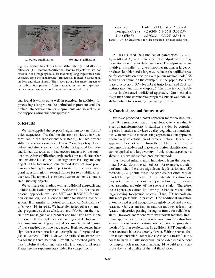
(a) before stabilization (b) after stabilization

Figure 2. Feature trajectories before stabilization (a) and after sta-

bilization (b). Before stabilization, feature trajectories are not

smooth in the image space. Note that many long trajectories were

extracted from the background. Trajectories related to foreground

are less and often shorter. Thus, background has more impacts to

the stabilization process. After stabilization, feature trajectories

become much smoother and the video is more stabilized.

and found it works quite well in practice. In addition, for

processing a long video, the optimization problem could be

broken into several smaller subproblems and solved by an

overlapped sliding window approach.

5. Results

We have applied the proposed algorithm to a number of

video sequences. The final results are best viewed in video

form (as in the supplementary material), but we present

stills for several examples. Figure 2 displays trajectories

before and after stabilization. As the background has more

and longer trajectories, it has greater impacts on the stabi-

lization. After stabilization, trajectories are much smoother

and the video is stabilized. Although there is a large moving

object in the foreground, our method does not have prob-

lem with finding the right object to stabilize. series of tem-

poral transformations. several frames for two stabilized se-

quences. The top one is considered easier as it only contains

small moving objects.

We compare our method with a traditional approach and

a video stabilization program, Deshaker [19]. For the tra-

ditional approach, we used SIFT and RANSAC for mo-

tion estimation, and a low-pass filter for motion compen-

sation. It is similar to motion estimation of Matsushita etal.’s work [14] in spirit. We have also tested other commer-

cial programs, such as iStabilize and iMovie, but their re-

sults are not as good as Deshaker and not listed here. None

of these methods implements inpainting and deblurring for

fair comparisons. Figures 4 and 5 show stabilized frames

of these methods on two sequences. Both sequences have

significant camera motion and complicated foreground ob-

ject movement. Table 1 shows the ratio of uncovered ar-

eas for these three methods. Overall, our method gives the

most stabilized videos and leaves the least uncovered areas.

Please see the supplementary video for comparisons.

sequence Traditional Deshaker Proposed

themepark (Fig 4) 4.2809% 5.1455% 3.0312%

skiing (Fig 5) 3.9608% 4.0559% 2.3641%Table 1. Un-coverage ratio for three methods on two sequences.

All results used the same set of parameters, λd = 1,

λs = 50 and λu = 1. Users can also adjust them to pay

more attention to what they care more. The adjustments are

intuitive: a smaller λd gives smoother motion; a larger λs

produces less blur and a larger λu reduces the unfilled area.

As for computation time, on average, our method took 2.58

seconds per frame on the examples in the paper. (51% for

feature detection, 26% for robust trajectories and 23% for

optimization and frame warping.) The time is comparable

to our implemented traditional approach. Our method is

faster than some commercial programs, but slower than De-

shaker which took roughly 1 second per frame.

6. Conclusions and future work

We have proposed a novel approach for video stabiliza-

tion. By using robust feature trajectories, we can estimate

a set of transformations to stabilize a video by consider-

ing user intention and video quality degradation simultane-

ously. In contrast to most existing approaches, our approach

doesn’t require estimation of camera motion. Hence, our

approach does not suffer from the problems with insuffi-

cient motion models and inaccurate motion classification. It

can be applied to a large variety of videos and experiments

show it is more robust than previous methods.

Our method inherits most limitations from the conven-

tional 2D-transform-based methods. For example, it under-

performs when there are significant depth variations. 3D

methods [2, 21] could avoid the problem but often rely on

unreliable depth estimation. For reliable depth estimation,

they often put restrictions on input videos by, for exam-

ple, assuming majority of the scene is static. Therefore,

these approaches often fail terribly to handle videos with

large moving foreground objects. Thus, 2D methods are

still more preferable in practice. One additional limitation

of our method is that it requires enough detected and tracked

features. Our current implementation requires at least five

feature trajectories passing through a frame for reliable re-

sults. However, for videos with insufficient features, tradi-

tional approaches suffer from inaccurate motion estimation

as well. Robust motion estimation for plain backgrounds is

worth of further exploration. In addition, SIFT detection is

more accurate but considerably slower. With the robust fea-

ture match procedure, other less accurate but faster features

could be used. Finally, incorporation of video enhancement

techniques such as motion inpainting [14] would greatly im-

prove the visual quality of the stabilized video.

1402

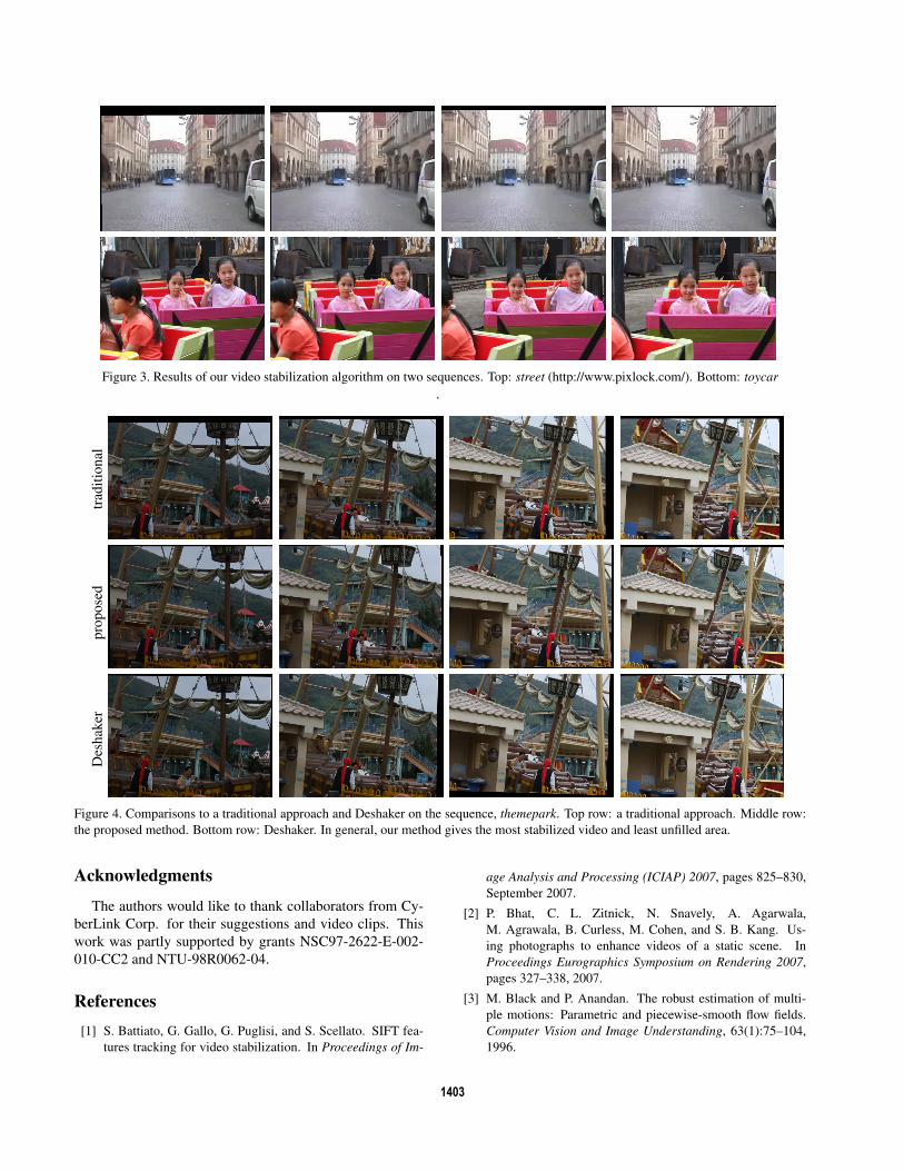
Figure 3. Results of our video stabilization algorithm on two sequences. Top: street (http://www.pixlock.com/). Bottom: toycar.

trad

itio

nal

pro

pose

dD

eshak

er

Figure 4. Comparisons to a traditional approach and Deshaker on the sequence, themepark. Top row: a traditional approach. Middle row:

the proposed method. Bottom row: Deshaker. In general, our method gives the most stabilized video and least unfilled area.

Acknowledgments

The authors would like to thank collaborators from Cy-

berLink Corp. for their suggestions and video clips. This

work was partly supported by grants NSC97-2622-E-002-

010-CC2 and NTU-98R0062-04.

References[1] S. Battiato, G. Gallo, G. Puglisi, and S. Scellato. SIFT fea-

tures tracking for video stabilization. In Proceedings of Im-

age Analysis and Processing (ICIAP) 2007, pages 825–830,

September 2007.

[2] P. Bhat, C. L. Zitnick, N. Snavely, A. Agarwala,

M. Agrawala, B. Curless, M. Cohen, and S. B. Kang. Us-

ing photographs to enhance videos of a static scene. In

Proceedings Eurographics Symposium on Rendering 2007,

pages 327–338, 2007.

[3] M. Black and P. Anandan. The robust estimation of multi-

ple motions: Parametric and piecewise-smooth flow fields.

Computer Vision and Image Understanding, 63(1):75–104,

1996.

1403

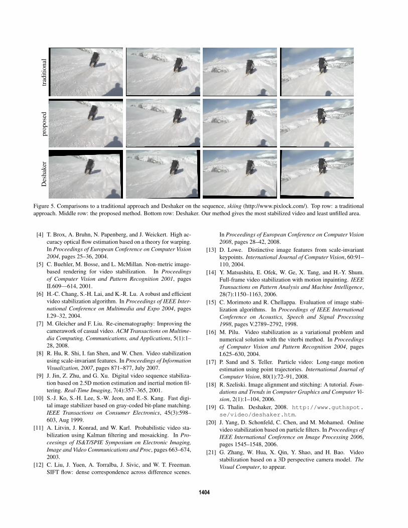
trad

itio

nal

pro

pose

dD

eshak

er

Figure 5. Comparisons to a traditional approach and Deshaker on the sequence, skiing (http://www.pixlock.com/). Top row: a traditional

approach. Middle row: the proposed method. Bottom row: Deshaker. Our method gives the most stabilized video and least unfilled area.

[4] T. Brox, A. Bruhn, N. Papenberg, and J. Weickert. High ac-

curacy optical flow estimation based on a theory for warping.

In Proceedings of European Conference on Computer Vision2004, pages 25–36, 2004.

[5] C. Buehler, M. Bosse, and L. McMillan. Non-metric image-

based rendering for video stabilization. In Proceedingsof Computer Vision and Pattern Recognition 2001, pages

II.609—614, 2001.

[6] H.-C. Chang, S.-H. Lai, and K.-R. Lu. A robust and efficient

video stabilization algorithm. In Proceedings of IEEE Inter-national Conference on Multimedia and Expo 2004, pages

I.29–32, 2004.

[7] M. Gleicher and F. Liu. Re-cinematography: Improving the

camerawork of casual video. ACM Transactions on Multime-dia Computing, Communications, and Applications, 5(1):1–

28, 2008.

[8] R. Hu, R. Shi, I. fan Shen, and W. Chen. Video stabilization

using scale-invariant features. In Proceedings of InformationVisualization, 2007, pages 871–877, July 2007.

[9] J. Jin, Z. Zhu, and G. Xu. Digital video sequence stabiliza-

tion based on 2.5D motion estimation and inertial motion fil-

tering. Real-Time Imaging, 7(4):357–365, 2001.

[10] S.-J. Ko, S.-H. Lee, S.-W. Jeon, and E.-S. Kang. Fast digi-

tal image stabilizer based on gray-coded bit-plane matching.

IEEE Transactions on Consumer Electronics, 45(3):598–

603, Aug 1999.

[11] A. Litvin, J. Konrad, and W. Karl. Probabilistic video sta-

bilization using Kalman filtering and mosaicking. In Pro-ceesings of IS&T/SPIE Symposium on Electronic Imaging,Image and Video Communications and Proc, pages 663–674,

2003.

[12] C. Liu, J. Yuen, A. Torralba, J. Sivic, and W. T. Freeman.

SIFT flow: dense correspondence across difference scenes.

In Proceedings of European Conference on Computer Vision2008, pages 28–42, 2008.

[13] D. Lowe. Distinctive image features from scale-invariant

keypoints. International Journal of Computer Vision, 60:91–

110, 2004.

[14] Y. Matsushita, E. Ofek, W. Ge, X. Tang, and H.-Y. Shum.

Full-frame video stabilization with motion inpainting. IEEETransactions on Pattern Analysis and Machine Intelligence,

28(7):1150–1163, 2006.

[15] C. Morimoto and R. Chellappa. Evaluation of image stabi-

lization algorithms. In Proceedings of IEEE InternationalConference on Acoustics, Speech and Signal Processing1998, pages V.2789–2792, 1998.

[16] M. Pilu. Video stabilization as a variational problem and

numerical solution with the viterbi method. In Proceedingsof Computer Vision and Pattern Recognition 2004, pages

I.625–630, 2004.

[17] P. Sand and S. Teller. Particle video: Long-range motion

estimation using point trajectories. International Journal ofComputer Vision, 80(1):72–91, 2008.

[18] R. Szeliski. Image alignment and stitching: A tutorial. Foun-dations and Trends in Computer Graphics and Computer Vi-sion, 2(1):1–104, 2006.

[19] G. Thalin. Deshaker, 2008. http://www.guthspot.se/video/deshaker.htm.

[20] J. Yang, D. Schonfeld, C. Chen, and M. Mohamed. Online

video stabilization based on particle filters. In Proceedings ofIEEE International Conference on Image Processing 2006,

pages 1545–1548, 2006.

[21] G. Zhang, W. Hua, X. Qin, Y. Shao, and H. Bao. Video

stabilization based on a 3D perspective camera model. TheVisual Computer, to appear.

1404