VIBRATIONAL SPECTRA AND n-BODY DECOMPOSITION ANALYSES OF WATER...
151
VIBRATIONAL SPECTRA AND n-BODY DECOMPOSITION ANALYSES OF WATER CLUSTERS by Jun Cui BS, Fudan University, China. 1995 MISM, Carnegie Mellon Univeristy, 2002 Submitted to the Graduate Faculty of Arts and Sciences in partial fulfillment of the requirements for the degree of Doctor of Philosophy University of Pittsburgh 2007
Transcript of VIBRATIONAL SPECTRA AND n-BODY DECOMPOSITION ANALYSES OF WATER...
VIBRATIONAL SPECTRA AND n-BODY DECOMPOSITION ANALYSES
OF WATER CLUSTERS
by
Jun Cui
BS, Fudan University, China. 1995
MISM, Carnegie Mellon Univeristy, 2002
Submitted to the Graduate Faculty of
Arts and Sciences in partial fulfillment
of the requirements for the degree of
Doctor of Philosophy
University of Pittsburgh
2007
UNIVERSITY OF PITTSBURGH
FACULTY OF ARTS AND SCIENCES
This dissertation was presented
by
Jun Cui
It was defended on
April 24, 2007
and approved by
Peter E. Siska, Ph.D.
Joseph J. Grabowski, Ph.D.
Jeffry D. Madura, Ph.D.
Dissertation Advisor: Kenneth D. Jordan, Ph.D.
ii
VIBRATIONAL SPECTRA AND N-BODY DECOMPOSITION ANALYSES OF
WATER CLUSTERS
Jun Cui
University of Pittsburgh, 2007
The hydrated proton lies at the heart of several key charge transport processes in
chemistry and biology, and yet the molecular level description of proton accommodation remains
elusive. Both H3O+ (so called Eigen) and (H2O···H···OH2)+ (so called Zundel) have long been
thought to play essential roles in the proton transfer process. We characterize the hydrated proton
with a “bottom up” approach to monitor the spectral evolution of the proton accommodation
motif as water molecules are sequentially added to the H3O+ ion. It is found that a highly
symmetrical structure is necessary to observe the Eigen ion. Small asymmetries in the hydration
structure around the H3O+ core result in preferential localization of the excess charge on one or
two of the hydrogen atoms. This extreme response to symmetry breaking readily explains the
lack of a crisp spectral signature of the hydrated proton in the bulk. Density functional theory is
used to study the relative stability of various isomers of (H2O)n · H+, n = 4-12, allowing for the
influence of vibrational zero point energy and finite temperature effects. Comparison of
experimental spectra with and without Ar tagging shows that the inclusion of Ar atoms has little
effect on the frequencies.
Two low-energy minima of (H2O)21 with very different H-bonding arrangements have
been investigated with the B3LYP density functional and RIMP2 methods, as well as with the
TIP4P, Dang–Chang, AMOEBA, and TTM2-F force fields. Insight into the role of many-body
iii

polarization for establishing the relative stability of the two isomers is provided by an n-body
decomposition of the energies calculated using the various theoretical methods.
iv
TABLE OF CONTENTS
TABLE OF CONTENTS............................................................................................................... V LIST OF TABLES.......................................................................................................................VII LIST OF FIGURES ................................................................................................................... VIII PREFACE.................................................................................................................................. XIII 1.0 INTRODUCTION ......................................................................................................... 1 2.0 SPECTRAL SIGNATURES OF HYDRATED PROTON VIBRATIONS IN WATER CLUSTERS..................................................................................................................................... 4
2.1 ABSTRACT .......................................................................................................... 4 2.2 INTRODUCTION ................................................................................................. 5 2.3 DISCUSSION........................................................................................................ 8
2.3.1 H+ · (H2O)4 ...................................................................................................... 8 2.3.2 H+ · (H2O)3 .................................................................................................... 13 2.3.3 H+ · (H2O)2 .................................................................................................... 14 2.3.4 H+ · (H2O)5 .................................................................................................... 14 2.3.5 H+ · (H2O)6 .................................................................................................... 15 2.3.6 H+ · (H2O)n, n=7, 8......................................................................................... 16
2.4 SUMMARY......................................................................................................... 16 2.5 ACKNOWLEDGEMENTS................................................................................. 17
3.0 FINITE TEMPERATURE EFFECTS AND ARGON ATOM PERTURBATIONS ON THE ENERGIES AND VIBRATIONAL SPECTRA OF PROTONATED WATER CLUSTERS 18
3.1 ABSTRACT ........................................................................................................ 18 3.2 INTRODUCTION ............................................................................................... 19 3.3 COMPUTATIONAL DETAILS ......................................................................... 20 3.4 RESULTS AND DISCUSSION.......................................................................... 21
3.4.1 Finite Temperature Effect ............................................................................. 21 3.4.2 Effect of Ar tagging ...................................................................................... 36
3.5 CONCLUSIONS ................................................................................................. 44 3.6 ACKNOWLEDGEMENTS................................................................................. 44
4.0 THEORETICAL CHARACTERIZATION OF THE (H2O)21 CLUSTER: APPLICATION OF AN N-BODY DECOMPOSITION PROCEDURE .................................... 45
4.1 ABSTRACT ........................................................................................................ 45 4.2 INTRODUCTION ............................................................................................... 46 4.3 COMPUTATIONAL DETAILS ......................................................................... 49 4.4 RESULTS AND DISCUSSION.......................................................................... 51
4.4.1 Energies of the Isomers................................................................................. 51 4.4.2 n-body Interaction Energies.......................................................................... 53
v

4.5 CONCLUSIONS ................................................................................................. 58 4.6 ACKNOWLEDGEMENTS................................................................................. 60
5.0 MANY BODY DECOMPOSITION STUDY OF THE (H2O)21 CLUSTER .............. 70 5.1 ABSTRACT ........................................................................................................ 70 5.2 INTRODUCTION ............................................................................................... 71 5.3 COMPUTATIONAL DETAILS ......................................................................... 72 5.4 RESULTS AND DISCUSSION.......................................................................... 73
5.4.1 n-body energy distribution for DD(20,1) subclusters ................................... 74 5.4.2 Structural analysis for typical tetramers ....................................................... 86
5.5 CONCLUSIONS ................................................................................................. 92 5.6 ACKNOWLEDGEMENTS................................................................................. 93
APPENDIX: MONITORING THE ACTIVITY OF BRAIN CHOLINERGIC SYSTEMS........ 94 BIBLIOGRAPHY....................................................................................................................... 133
vi

LIST OF TABLES
Table 1: Comparison of the calculated and measured OH-stretch vibrational frequencies for the H+ · (H2O)n, n = 2 - 8 clustersa, d .......................................................................................... 11
Table 2. n-body interaction energies (kcal/mol) for the TIP4P-gm(21) and DD(20,1) isomers of (H2O)21
a................................................................................................................................ 67 Table 3. 4-body interaction energies (kcal/mol) of selected tetramers from DD(20,1)a,b ............ 68 Table 4. 3-body interaction energies (kcal/mol) of selected trimers from DD(20,1)a .................. 69
vii
LIST OF FIGURES
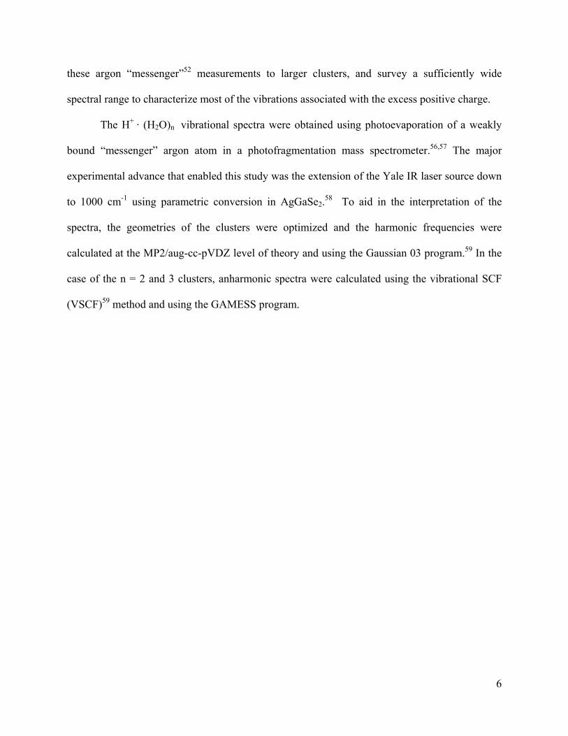
Figure 1. Minimum energy structures of H+ · (H2O)n where n = 2 – 6. Geometries were calculated at the MP2/aug-cc-pVDZ level of theory. Blue arrows depict the normal mode displacement vectors associated with the lowest energy stretching motion involving the extra proton. ........................................................................................................................... 7
Figure 2. Comparison of the OH asymmetric stretch (νasym) and asymmetric bending (νbend) bands of (A) bare H3O+ 61,62 and (B) H+ · (H2O)4. The calculated harmonic spectrum [MP2/aug-cc-pVDZ level, 0.955 scaling] of H+ · (H2O)4 is displayed by bars, where the Eigen core stretches are highlighted in red. ........................................................................... 9
Figure 3. Argon predissociation spectra of H+ · (H2O)n, n = 2 – 11, with n increasing down the figure. Dangling waters attached to the exterior of the cluster network are identified by sharp features and are assigned to the HOH intramolecular bend (νbend), symmetric (νs), and asymmetric (νa) OH stretches. The bands most closely associated with the motions of hydrogen atoms bearing the excess charge are highlighted in red. Note that this feature first evolves toward higher energy as the excess charge undergoes most delocalization at n = 4 (trace C), but then returns to lower energy as more water molecules are added. The persistence of the intact Zundel signature (νz) in the n= 6 – 8 spectra indicates that the excess charge is primary retained on one strongly shared proton in this size range. Bands derived from the OH stretches bridging the core ions to the first hydration shell are highlighted in blue. .............................................................................................................. 10
Figure 4. Relative electronic energy and free energy of the H+ · (H2O)4 cluster (in kcal/mol). The electronic energies of the isomers are compared with and without vibrational zero-point energy correction. The dependences of free energy over temperature are also compared. The energy values are the difference between the energy of each isomer and the lowest energy under the conditions displayed at the X-axis. Each colored curve represents one isomer. The isomer structures are displayed at the top........................................................ 22
Figure 5. Relative electronic energies and free energyies of typical H+ · (H2O)5 isomers (in kcal/mol). The electronic energies of the isomers are compared with and without vibrational zero-point energy correction. The dependences of free energy over temperature are also compared. The energy values are the difference between the energy of each isomer and the lowest energy under the conditions displayed at the X-axis. Each colored curve represents one isomer. The isomer structures are displayed at the top................................ 24
Figure 6. Relative electronic energies and free energies of typical H+ · (H2O)6 isomers (in kcal/mol). The electronic energies of the isomer are compared with and without zero-point vibrational energy correction. The dependences of free energy over temperature are also compared. The energy values are the difference between the energy of each isomer and the
viii

lowest energy under the conditions displayed at the X-axis. Each colored curve represents one isomer. The isomer structures are displayed at the top. ................................................ 26
Figure 7. Relative electronic energies and free energies of typical H+ · (H2O)7 isomers (in kcal/mol). The electronic energies of the isomers are compared with and without zero-point vibrational energy correction. The dependences of free energy over temperature are also compared. The energy values are the difference between the energy of each isomer and the lowest energy under the conditions displayed at the X-axis. Each colored curve represents one isomer. The isomer structures are displayed at the top................................ 30
Figure 8. Relative electronic energies and free energies of typical H+ · (H2O)8 isomers (in kcal/mol). The electronic energies of the isomers are compared with and without zero-point vibrational energy correction. The dependences of free energy over temperature are also compared. The energy values are the difference between the energy of each isomer and the lowest energy under the conditions displayed at the X-axis. Each colored curve represents one isomer. The isomer structures are displayed at the top................................ 31
Figure 9. Relative electronic energies and free energies of typical H+ · (H2O)9 isomers (in kcal/mol). The electronic energies of the isomers are compared with and without zero-point vibrational energy correction. The dependences of free energy over temperature are also compared. The energy values are the difference between the energy of each isomer and the lowest energy under the conditions displayed at the X-axis. Each colored curve represents one isomer. The isomer structures are displayed at the top................................ 32
Figure 10. Relative electronic energies and free energies of typical H+ · (H2O)10 isomers (in kcal/mol). The electronic energies of the isomers are compared with and without zero-point vibrational energy correction. The dependences of free energy over temperature are also compared. The energy values are the difference between the energy of each isomer and the lowest energy under the conditions displayed at the X-axis. Each colored curve represents one isomer. The isomer structures are displayed at the top................................ 33
Figure 11. Relative electronic energies and free energies of typical H+ · (H2O)11 isomers (in kcal/mol). The electronic energies of the isomers are compared with and without zero-point vibrational energy correction. The dependences of free energy over temperature are also compared. The energy values are the difference between the energy of each isomer and the lowest energy under the conditions displayed at the X-axis. Each colored curve represents one isomer. The isomer structures are displayed at the top................................ 34
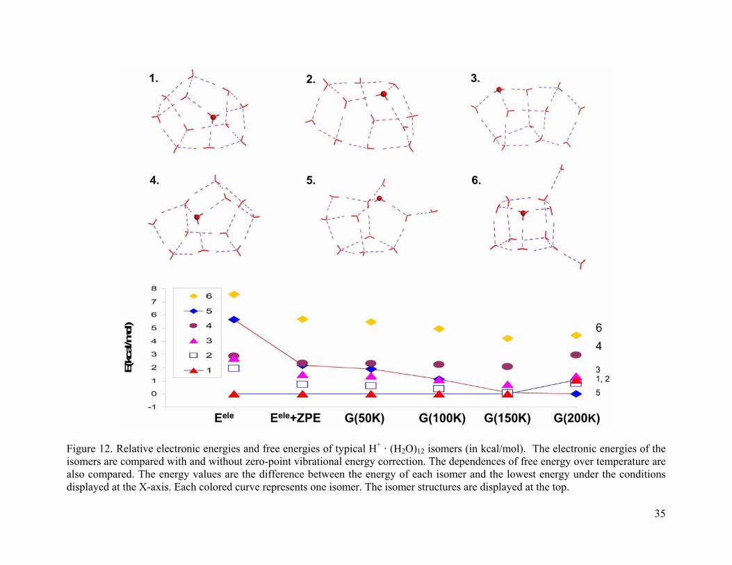
Figure 12. Relative electronic energies and free energies of typical H+ · (H2O)12 isomers (in kcal/mol). The electronic energies of the isomers are compared with and without zero-point vibrational energy correction. The dependences of free energy over temperature are also compared. The energy values are the difference between the energy of each isomer and the lowest energy under the conditions displayed at the X-axis. Each colored curve represents one isomer. The isomer structures are displayed at the top................................ 35
Figure 13. Structures and relative energies (in kcal/mol) of (H2O)6 · H+ · Ar cluster for the three lowest energy isomers of (H2O)6 · H+ (6A, 6B and 6C). The electronic energies of the isomers are compared with vibrational zero-point energy correction. The energy values are the difference between the energy of each isomer and the energy of 6A-1. The relative energies of the three (H2O)6 · H+ structures are: 0.0 (6A), 0.30 (6B), 0.69 (6B) kcal/mol. Note the attachment of Ar atom does not change the energy ordering of 6A, 6B, 6C and the position of Ar atom attachment has a small effect on the energy........................................ 37
ix
Figure 14. Structures and relative energies (in kcal/mol) of (H2O)7 · H+ · Ar cluster for the three lowest energy isomers of (H2O)7 · H+ (7A, 7B and 7C). The electronic energies of each isomer are compared with vibrational zero-point energy correction. The energy values are the difference between the energy of each isomer and the energy of 7A-1. The relative energies of the three (H2O)7 · H+ structures are: 0.0 (7A), 0.51 (7B), 1.44 (7B). Note the attachment of an Ar atom does not change the energy ordering of 7A, 7B, 7C and the position of Ar attachment has a small effect on the energy................................................. 38
Figure 15. Comparison of predissociation spectra of H+ · (H2O)n, n = 3 – 5 with and without Ar tagging, with n increasing from bottom to top. (Spectra provided by Prof. M. Duncan).... 42
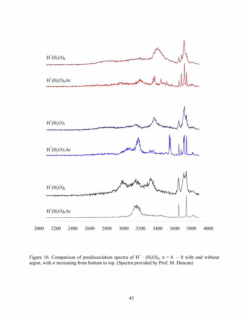
Figure 16. Comparison of predissociation spectra of H+ · (H2O)n, n = 6 – 8 with and without argon, with n increasing from bottom to top. (Spectra provided by Prof. M. Duncan)....... 43
Figure 17. RIMP2/aug-cc-pVDZ optimized geometries of the (a) DD(20,1) and (b) TIP4P-gm(21) isomers of (H2O)21 and of the (c) D(19,1), (d) pentagonal prism [PP(20)], and (e) “perfect” dodecahedron [PD(20)] isomers of (H2O)20......................................................... 61
Figure 18. Interaction energies for the DD(20,1) and TIP4P-gm(21) isomers of (H2O)21 and of various forms of (H2O)20 calculated using the TIP4P, DC, TTM2-F, AMOEBA, B3LYP/aug-cc-pVTZ(-f), and RIMP2/aug-cc-pVTZ(-f) methods...................................... 62
Figure 19. Cumulative 2-body interaction energies vs. distance L for the TIP4P-gm(21) and DD(20,1) isomers of (H2O)21. .............................................................................................. 63
Figure 20. Cumulative 3-body interaction energies vs. distance for the TIP4P-gm(21) and DD(20,1) isomers of (H2O)21. .............................................................................................. 64
Figure 21. Cumulative 4-body interaction energies vs. distance for the TIP4P-gm(21) and DD(20,1) isomers of (H2O)21. .............................................................................................. 65
Figure 22. Tetramers selected from the RIMP2/aug-cc-pVDZ optimized structure of the DD(20,1) isomer of (H2O)21. ............................................................................................... 66
Figure 23. Difference in 2-body energy obtained from (a) MP2 and HF, (b) MP2 and B3LYP, and (c) MP2 and AMOEBA methods vs. distance for dimers from the DD(20, 1) isomer of (H2O)21. The aug-cc-pVTZ basis set is used for the MP2 and HF methods, and aug-cc-pVDZ for B3LYP method. .................................................................................................. 77
Figure 24. Difference in 3-body energy obtained from (a) MP2 and HF, (b) MP2 and B3LYP, and (c) MP2 and AMOEBA methods vs. distance for trimers from the DD(20, 1) isomer of (H2O)21. The aug-cc-pVTZ basis set is used for the MP2 and HF methods, and aug-cc-pVDZ for B3LYP method. .................................................................................................. 79
Figure 25. Difference in 4-body energy obtained from MP2 and HF methods vs. distance for tetramers from DD(20, 1) isomer of (H2O)21. The aug-cc-pVTZ basis set is used for the MP2 and HF methods. The DD(20, 1) isomer of (H2O)21 was optimized at the MP2 level of theory and aug-cc-pVDZ basis set. ...................................................................................... 83
Figure 26. Difference in 4-body energy obtained from (a) MP2 and B3LYP, and (b) MP2 and AMOEBA methods vs. distance for tetramers from DD(20, 1) isomer of (H2O)21. The aug-cc-pVTZ basis set is used for the MP2 method, and aug-cc-pVDZ for B3LYP method. The DD(20, 1) isomer of (H2O)21 was optimized at the MP2 level of theory and aug-cc-pVDZ basis set. ............................................................................................................................... 85
Figure 27. (a) Structure of tetramer 3-5-11-15 extracted from the DD(20, 1) isomer of (H2O)21. (b) 4-body energy change with distance between water 3 and 15. The energies are obtained from the MP2, Hartee Fock, B3LYP and AMOEBA methods. The aug-cc-pVTZ basis set
x
is used for the MP2, HF and B3LYP methods. The DD(20, 1) isomer of (H2O)21 was optimized at the MP2 level of theory with the aug-cc-pVDZ basis set. .............................. 89
Figure 28. (a) Structure of tetramer 9-12-14-19 extracted from the DD(20, 1) isomer of (H2O)21. (b) 4-body energy change with distance between water 19 and 9. The energies are obtained from the MP2, Hartee Fock, B3LYP and AMOEBA methods. The aug-cc-pVTZ basis set is used for the MP2, HF and B3LYP methods. The DD(20, 1) isomer of (H2O)21 was optimized at the MP2 level of theory with the aug-cc-pVDZ basis set. .............................. 90
Figure 29. 4-body induction energy change with distance between water 3 and 15 (tetramer structure shown in Figure 27(a)). The decomposed energies were obtained with the KM and RVS methods. ............................................................................................................... 91
Figure 30 Scheme of acetylcholine release and choline reuptake at cholinergic neuron terminals. TTX is tetrodotoxin.............................................................................................................. 99
Figure 31. (a) Schematic representation of the sequential reactions that occurred at the choline bienzyme microsensor. Structures of (b) the redox polymer and (c) the crosslinker that were used to immobilize the enzymes onto the carbon fiber microelectrode surface. ...... 101
Figure 32. Scheme of microsensors and micropipet positions for local infusion experiments in the striatum of the rat brain. Choline microsensor was used as the working microsensor. It was implanted side by side with background microsensor. Background microsensors were made exactly the same as choline microsensors except without choline oxidase. ............ 107
Figure 33. Amperometric calibration curves obtained with choline microsensors at 37oC, without (filled circles) and with (empty circles) 400 µM ascorbic acid (a) before in vivo experiment. (b) after in vivo experiment. .......................................................................... 109
Figure 34. Traces of current recorded during local injection experiments using choline microsensors (Ch) and background microsensors (bkg) implanted in rat striatum. Responses of microsensors after local injection of (a) 10 mM, 200 nl choline. (b) 200 nl aCSF. (c) 4 mg/ml, 800 nl choline oxidase. The experiments were operated at -100 mV vs. Ag/AgCl. The horizontal bars represent the start and end of injection. The vertical bars show choline concentration obtained according to post calibration of microsensors........ 111
Figure 35. Traces of current recorded during local infusion of 100 µM, 200 nl tetrodotoxin (TTX) with choline microsensor (Ch) and background microsensor (bkg) implanted side by side in tha rat striatum. The experiments were operated at -100 mV vs. Ag/AgCl. The horizontal bar represents the start and end of infusion. The vertical bar represents choline concentration obtained according to the post calibration of microsensors. ....................... 113
Figure 36. Calibration curves for choline microsensor with (filled circles) and without (empty circles) 100 µM tetraodotoxin (TTX). The microsesnors were operated at -100 mV vs. Ag/AgCl at 37oC. ............................................................................................................... 114
Figure 37. Traces of current recorded during local infusion with choline microsensors (Ch) and background microsensors (bkg) implanted side by side in the rat striatum. (a) Responses to local infusion of 800 nl aCSF. (b) 500 µM, 800 nl neostigmine. The experiments were operated at -100 mV vs. Ag/AgCl. The horizontal bars represent the start and end of infusion. The vertical bars show choline concentration obtained according to post calibration of microsensors. ............................................................................................... 116
Figure 38. Amperometric calibration curve for choline microsensor with (empty circles) and without (filled circles) 500 µM neostigmine. The microsensor was operated at 37oC...... 117
Figure 39. Amperometric calibration curve for glucose microsensor made with glucose oxidase concentration of 2 mg/ml. The calibration was done at 37oC before in vivo experiment. 119
xi
Figure 40. Amperometric calibration curves for glucose microsensors made with glucose oxidase concentration of 75 µg/ml. The calibration wre made with (empty circles) and without (filled circles) 400 µM ascorbic acid at 37oC (a) before in vivo experiment. (b) after in vivo experiment.......................................................................................................................... 120
Figure 41. Traces of current recorded during local infusion with glucose microsensor and background microsensor (bkg) implanted side by side in the rat striatum. Responses to local infusion of (a) 200 nl aCSF. (b) 1 M, 200 nl glucose. (c) 4 mg/ml, 800 nl glucose oxidase. The experiments were operated at -100 mV vs. Ag/AgCl. The horizontal bars represent the start and end of injection. The vertical bars show glucose concentration obtained according to post calibration of microsensors..................................................... 122
Figure 42. Traces of current recorded during local infusion of 100 µM, 200 nl TTX with glucose microsensor and background microsensor (bkg). The experiments were operated at -100 mV vs. Ag/AgCl. The horizontal bar represents the start and end of injection. The vertical bar shows glucose concentration obtained according to post calibration of microsensors.124
Figure 43. Amperometric calibration curves for glucose microsensor with (empty circles) and without (filled circles) 100 µM TTX at 37oC after in vivo experiment. The microsensors were operated at -100 mV vs. Ag/AgCl at 37oC................................................................ 126
Figure 44. Traces of current recorded during local infusion of (a) 800 nl aCSF. (b) 500 µM, 800 nl neostigmine with glucose microsensor and background microsensor (bkg) implanted side by side in the rat striatum. The experiments were operated at -100 mV vs. Ag/AgCl. The horizontal bars represent the start and end of injection. The vertical bars show glucose concentration obtained according to post calibration of microsensors.............................. 127
Figure 45. Amperometric calibration curves for glucose microsensors with (empty circles) and without (filled circles) 500 µM neostigmine after in vivo experiment. The microsensors were operated at -100 mV vs. Ag/AgCl at 37oC................................................................ 128
xii

PREFACE
Wow! I am finally here!
First, I would like to thank my advisor, Prof. Kenneth D. Jordan, for his great mentorship
and patience in the past years. I feel lucky to have him as my Ph.D. advisor. From him, I learned
not only the science, but also how to be a great scientist.
I would like to thank my past and current friends in the Jordan group for their friendship
and great help, especially Valerie McCarthy, Kadir Diri, and Hanbin Liu.
Finally, I want to thank my parents and husband for their endless patience and support
while waiting for me to get a real job. Mom and dad, I am getting there!
xiii
1.0 INTRODUCTION
Proton transfer through hydrogen bonding plays essential roles in many chemical
processes such as atmosphere, solution phases and biological systems.1-7 The high mobility of
protons in liquid water involves the chemical exchange of proton along the charge transfer path.8-
12 Protonated water clusters can serve as model systems to study proton transport in various
environments. For example, the clusters can also act as acidic microsolvation matrices to
catalyze reactions in liquids.13 The OH groups on the cluster surfaces can heterogeneously
catalyze chlorine which is related to the ozone hole over Antarctica.14,15 Protonated water
clusters are among the most thoroughly studied cluster ions in the gas phase since they were
found by mass spectrometry. There has been active research on the structures, energetics, and
ion-molecule reactions.16-23
There has been major interest in the nature of the proton in water. Two major models
have been proposed, one is the formation of H9O4+ with a H3O+ core strongly hydrogen-bonded
to 3 water molecules,8 the other is a H5O2+ complex in which the proton shared between two H2O
molecules.24 Much of the early work attempted to determine the structure of the clusters by X-
ray or neutron diffraction.25 Evidence of both H3O+ (so called “Eigen” structure) and H2O · H+ ·
H2O (so called “Zundel” structure) has been found.
Spectroscopic studies of gas phase hydrated proton clusters will improve our knowledge
about the nature of excess protons in liquid water.9,26 However, obtaining the experimental
1
vibrational spectra of protonated water clusters is very challenging. Large density of states
dilutes the population in any given state. This problem can be solved by vibrational
predissociation or multiphoton dissociation process. For weakly bound ionic clusters, excitation
of high frequency vibrational degrees of freedom induces dissociation allowing for the
determination of vibrational predissociation spectra. When the binding energy of protonated
water cluster exceeds the vibrational quanta, the predissociation process will not occur after
vibrational excitation. A weakly bound messenger such as H2 and Ne can be attached to the
cluster. The vibrational excitation of the cluster detaches the messenger and makes vibrational
predissociation spectra possible. More recently, Ar predissociation spectroscopy has been used to
acquire the spectra in the low energy region to characterize the intramolecular bending and
bridging proton motions.26,27
Gas phase mass spectroscopic studies were carried out on hydrated protons by Searcy and
Fenn in 1974 to detect the formation of (H2O)n · H+ (n = 1-28).28 In 1970s, Kebarle and
coworkers29,30 pioneered the hydration energy measurements and obtained the single water
binding energies of (H2O)n · H+ to be 31.6, 19.5 and 17.9 kcal/mol for n = 2, 3, and 4,
respectively. Newton and Ehrenson31,32 carried elaborate calculations, and Schwartz33 obtained
the first infrared absorption spectra of proton hydrates in a cold static cell with cluster sizes of n
= 3-5 from 2000-4000 cm-1 at 40 cm-1 resolution. In 1989, Lee et al. obtained the gas phase
vibrational spectra of H3O+ · (H2O)n (n=1-3) in the range of 3550-3800 cm-1 with multiphoton
dissociation method and characterized the Zundel structure.34 Jiang et al. reported the infrared
spectra of (H2O)n · H+ (n=5-8) in the 2700-3900 cm-1 region.
Also, numerous theoretical studies, such as molecular dynamics and ab initio electronic
structure calculations,23,35 have been carried out along with experimental studies36 to determine
2

the structure and vibrational spectra of protonated water clusters.16,37,38 However, the location of
the excess proton and a detailed understanding of the structure observed in the vibrational spectra
have remained elusive,39 and studies in this area are far from complete.
3
2.0 SPECTRAL SIGNATURES OF HYDRATED PROTON VIBRATIONS IN WATER
CLUSTERS
This work was published as:
Headrick J., Diken E.G., Walters R.S., Hammer N.I., Christie R.A., Cui J., Myshakin E.M.,
Duncan M.A., Johnson M.A., Jordan K.D., Science 308 1765-1769 (2005).27
2.1 ABSTRACT
The hydrated proton lies at the heart of several key charge transport processes in
chemistry and biology,40-44 and yet the molecular level description of proton accommodation
remains elusive.8,10,12,24,35,45-48 Although virtually every introductory chemistry text posits that the
dominant speciation occurs as “hydronium” (H3O+, also called the Eigen8 core), this picture is
certainly too simplistic. Indeed, an alternative limiting form proposed by Zundel24
(H2O···H···OH2)+ has long been thought to play an essential role, and the broad infrared
absorptions of the aqueous proton at 1250, 1760 and 3020 cm-1 have been assigned in the context
of both Eigen and Zundel species over the years.49-51 Recently, a qualitatively different picture
has emerged as contemporary theoretical treatments point to a scenario where, at finite
temperature, the excess proton is associated with an ensemble of intermediate structures that
4
continuously evolve according to fluctuations in the surrounding liquid.35,48 This model does not
require persistent structural motifs, like the Eigen and Zundel ions, separated by barriers. In this
chapter, we characterize the hydrated proton with a “bottom up” approach, where we capitalize
on recent advances in laser generation of infrared light to monitor the spectral evolution of the
proton accommodation motif as water molecules are sequentially added to the hydronium ion.
2.2 INTRODUCTION
Infrared spectra of bare H+ · (H2O)n clusters in the OH stretching region (2800–3900cm-1,
with inconsistent coverage below 2800 cm-1) have already been reported, and the observed bands
are mostly attributed to water molecules remote from the proton.16,23,36,52,53 Dangling water
molecules attached to the exterior of a hydrogen bonding network, for example, produce sharp
bands arising from the symmetric (υs) and asymmetric (υa) stretches of the non-bonded OH
groups. Theoretical analysis of these high-energy patterns indicated that the clusters evolve
through the series of structures illustrated in Figure 1, where the n = 2 and 6 clusters were found
to be based on a Zundel motif, while the n = 3 – 5 clusters contained an embedded Eigen core.
The motions associated with the proton isolated in these various structures occur at much
lower spectral energies than available in the early studies, and consequently, recent work has
concentrated on extending the spectral range below 2100 cm-1. Spectra in this crucial lower
energy region (600 – 1900 cm-1) have been obtained for the H5O2+ ion,9,54 and although the
spectra of the bare complexes were quite complex, a much simpler spectrum was obtained when
H5O2+ was cooled by attachment of weakly bound argon atoms.55 In the present study, we extend
5
these argon “messenger”52 measurements to larger clusters, and survey a sufficiently wide
spectral range to characterize most of the vibrations associated with the excess positive charge.
The H+ · (H2O)n vibrational spectra were obtained using photoevaporation of a weakly
bound “messenger” argon atom in a photofragmentation mass spectrometer.56,57 The major
experimental advance that enabled this study was the extension of the Yale IR laser source down
to 1000 cm-1 using parametric conversion in AgGaSe2.58 To aid in the interpretation of the
spectra, the geometries of the clusters were optimized and the harmonic frequencies were
calculated at the MP2/aug-cc-pVDZ level of theory and using the Gaussian 03 program.59 In the
case of the n = 2 and 3 clusters, anharmonic spectra were calculated using the vibrational SCF
(VSCF)59 method and using the GAMESS program.
6
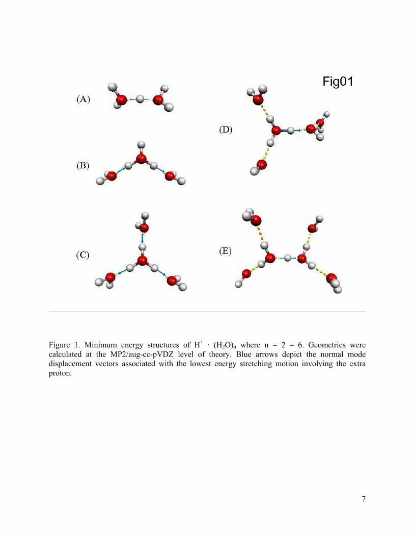
Figure 1. Minimum energy structures of H+ · (H2O)n where n = 2 – 6. Geometries were calculated at the MP2/aug-cc-pVDZ level of theory. Blue arrows depict the normal mode displacement vectors associated with the lowest energy stretching motion involving the extra proton.
7
2.3 DISCUSSION
2.3.1 H+ · (H2O)4
We begin our discussion with H+ · (H2O)4 which has a minimum energy structure
well described as an H3O+ Eigen core symmetrically solvated by three “dangling” water
molecules (Figure 1c). The measured and calculated (scaled harmonic frequencies) spectra of H+
· (H2O)4 are presented in Figure 2. Most importantly, the spectrum displays a broad, strong band
at 2665 cm-1, in agreement with the predicted location of the asymmetric OH stretching
vibrations of an intact Eigen core. Thus, the first solvent shell acts to red-shift the intrinsic OH
stretching motions of the isolated H3O+ ion60 by over 860 cm-1, just below the range scanned in
previous studies of this system. Several transitions are also recovered in the lower energy region.
The sharp feature at 1620 cm-1 can be readily assigned to the HOH intramolecular bends of the
dangling water molecules, and the unresolved feature emerging at 1045 cm-1 is traced to the
symmetric bending motion of the H3O+ ion core along its principle axis. Interestingly, the
broader features near 1760 cm-1 and 1900 cm-1, just above the bends in isolated H3O+,61 are
likely due to this type of motion in the charged center, but are the only major features not
qualitatively anticipated at the harmonic level.
8
Figure 2. Comparison of the OH asymmetric stretch (νasym) and asymmetric bending (νbend) bands of (A) bare H3O+ 61,62 and (B) H+ · (H2O)4. The calculated harmonic spectrum [MP2/aug-cc-pVDZ level, 0.955 scaling] of H+ · (H2O)4 is displayed by bars, where the Eigen core stretches are highlighted in red.
9
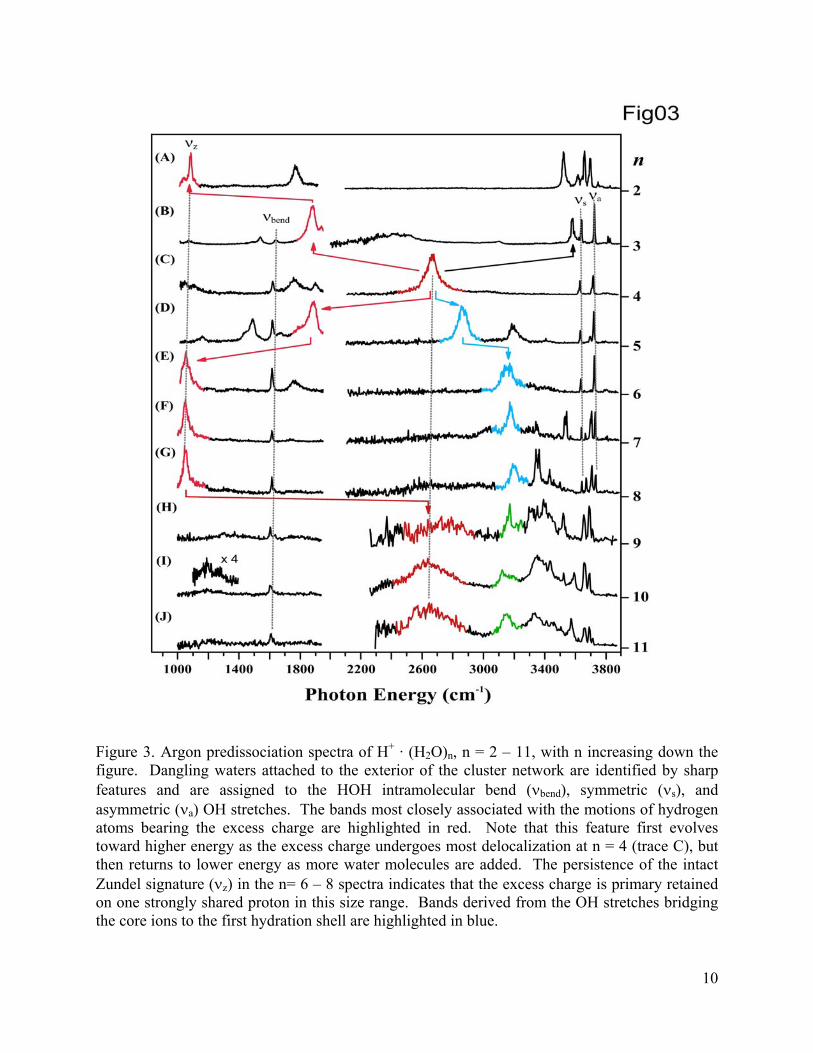
Figure 3. Argon predissociation spectra of H+ · (H2O)n, n = 2 – 11, with n increasing down the figure. Dangling waters attached to the exterior of the cluster network are identified by sharp features and are assigned to the HOH intramolecular bend (νbend), symmetric (νs), and asymmetric (νa) OH stretches. The bands most closely associated with the motions of hydrogen atoms bearing the excess charge are highlighted in red. Note that this feature first evolves toward higher energy as the excess charge undergoes most delocalization at n = 4 (trace C), but then returns to lower energy as more water molecules are added. The persistence of the intact Zundel signature (νz) in the n= 6 – 8 spectra indicates that the excess charge is primary retained on one strongly shared proton in this size range. Bands derived from the OH stretches bridging the core ions to the first hydration shell are highlighted in blue.
10
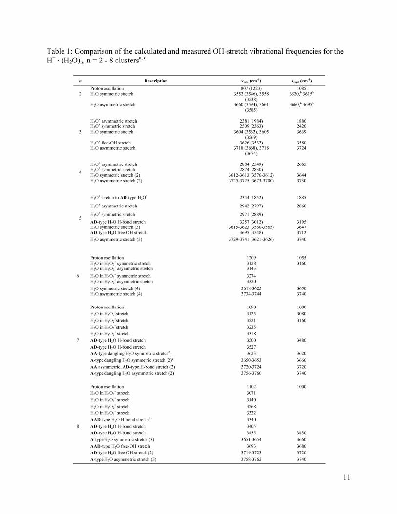
Table 1: Comparison of the calculated and measured OH-stretch vibrational frequencies for the H+ · (H2O)n, n = 2 - 8 clustersa, d
11

a For the theoretical results, anharmonic frequencies, where available are reported in parentheses. All other values are from harmonic calculations, unscaled in the case of the shared proton in the two Zundel ions and scaled by 0.955 in all other cases. b The observed OH stretch splittings are induced by the argon “messenger” atom. Our results correlate well with those reported in Ref. 19, where the “messenger” was H2. c A-type H2O molecules accept a hydrogen-bond. AA-type H2O molecules accept two hydrogen-bonds. AD-type H2O molecules accept and donate a hydrogen-bond. AAD-type H2O molecules accept two and donate one hydrogen-bond. d. H+ · (H2O)n, n = 7, 8 clusters use harmonic calculations (Becke3LYP with 6-31+g(d) basis set) and scaled by 0.975.
12
2.3.2 H+ · (H2O)3
Having established the spectral signature of the symmetrically hydrated Eigen
species, we turn our attention to the evolution of the spectra as water molecules are removed
from and added to this complete hydration shell, effectively mimicking rudimentary solvent
fluctuations. The n = 2 – 8 spectra are presented in Figure 3. First, note the persistence of the
sharp intramolecular bending band due to the dangling water molecules (~1620 cm-1), and the
presence of two to four non-bonded OH stretches centered near 3700 cm-1. The latter bands
were analyzed earlier,23,52,53 and here we are primarily interested in the broader bands associated
with stretching motions of the proton defect (which can be delocalized over up to three protons),
highlighted in red. Most of these occur below 2100 cm-1 and are reported here for the first time.
These strong absorptions are scattered throughout the low energy region in a very size dependent
fashion.
To unravel the information contained in these spectra, we first consider removing
a water molecule from the fully hydrated Eigen core to form H+ · (H2O)3. Although the resulting
cluster was structurally characterized as an Eigen-based species (Figure 1b), the 2665 cm-1
signature band of the Eigen cation is absent from its spectrum (Figure 3b). Instead, three strong
bands emerge at 1880, 2430, and 3580 cm-1. The calculations trace this pattern to a remarkably
strong (~1700 cm-1) splitting of the closely spaced bands in the partially hydrated Eigen ion.
Thus, the lower two of these transitions (highlighted in red) arise from the stretches of hydrated
protons while the higher frequency band involves the unsolvated proton stretch on the H3O+
core, which falls close to the OH stretch in bare H3O+.60 Interestingly, unlike the theoretical
situation in H+ · (H2O)4, anharmonic corrections are required to qualitatively recover the extent
13
of the red-shift displayed by the lower energy transition in the H+ · (H2O)3 spectrum. Removal
of one water molecule from the complete hydration shell thus leads to concentration of the
excess charge onto two shared protons, pulling the two solvating water molecules closer to the
Eigen core and thus red-shifting the associated OH stretch bands.
2.3.3 H+ · (H2O)2
Removal of a second water molecule from H+ · (H2O)4 creates the isolated Zundel ion,
[(H2O···H···OH2)+,(Figure 1a)], which has recently been reported and discussed in detail.55 Its
infrared spectrum (Figure 3a) is dominated by a strong transition at 1085 cm-1, arising from
oscillation of the shared proton, with a higher energy transition at 1770 cm-1, assigned to the out-
of-phase bending vibrations of the flanking water molecules. In going to the Zundel structure,
the ~ 800 cm-1 incremental red-shift of the bands associated with the excess positive charge is
about the same at that displayed upon removal of the first water molecule from the fully hydrated
Eigen cation. The important point here is that surprisingly large spectral shifts are driven by
changes in the hydration environment.
2.3.4 H+ · (H2O)5
Having explored the evolution of H+(H2O)n starting with the Eigen ion H+(H2O)4
and progressing to the Zundel ion H5O2+, we turn to the alternative situation where we
systematically add (nominally second shell) water molecules to H+(H2O)4. The vibrational
spectrum of H+ · (H2O)5 is presented in Figure 3d. Three sharp bands are observed in the high
energy non-bonded OH stretch region, consistent with the Eigen-like structure shown in Figure
14
1d. However, broader features emerge that are unique to this cluster, with an intense band about
200 cm-1 above the 2665 cm-1 signature absorption of the H+(H2O)4 Eigen ion. This might, at
first glance, suggest an unusual blue-shift upon solvation, but note that two new bands also
appear at lower energy (1490 cm-1 and 1885 cm-1). This pattern again raises the possibility that
the nearly degenerate Eigen vibrations are strongly split upon addition of a fourth water
molecule, much as they were upon removal of water molecule to form H+(H2O)3.
The harmonic calculations for the H+ · (H2O)5 structure (Figure 1d) anticipate a splitting
of the Eigen vibrations, but severely underestimate the effect with the three OH stretch vibrations
of the Eigen core predicted to occur at 2344, 2944, and 2971 cm-1. The two blue-shifted
transitions are clearly derived primarily from the vibrations of the two protons of the Eigen core
toward dangling water molecules in the first hydration shell. The third OH stretch of the Eigen
core, while predicted to red-shift as the proton becomes solvated by a water dimer, falls 459 cm-1
above the intense line observed at 1885 cm-1. The strong red shift of this vibration is thus a
consequence of excess charge concentration on the proton with two hydration shells coupled
with pronounced vibrational anharmonicity, comparable to the situation noted above for
H+(H2O)3.
2.3.5 H+ · (H2O)6
The addition of a second water molecule to H+ · (H2O)4 actually creates a favorable
situation for capturing the symmetrical Zundel ion (Figure 1e) within a complete first hydration
shell, and this arrangement was, in fact, identified in an earlier temperature-dependent study of
its non-bonded OH stretches.63 This structure can be viewed as further stabilizing the
preferentially hydrated proton in H+ · (H2O)5 such that it becomes equally shared between two
15
oxygen atoms. The resulting H+ · (H2O)6 spectrum (Figure 3e) has a very strong transition at
1055 cm-1, appearing in almost exactly the same location as the transition associated with
oscillation of the bridging proton in the isolated Zundel ion! Thus, the characteristic signature of
the local, shared proton motion is virtually unperturbed upon formation of its hydration shell,
unlike the situation in the more charge-delocalized Eigen arrangement, where the H3O+
stretching bands shift by almost 860 cm-1 upon hydration (i.e., in going from H3O+ to H+(H2O)4).
2.3.6 H+ · (H2O)n, n=7, 8
One is naturally curious as to whether this spectral evolution is oscillatory with
increasing hydration number, and to address this issue we carried out a survey of the n = 7 and 8
clusters with the results included in traces 3f and g. Remarkably, once the Zundel signature is
recovered at n = 6, it is not only maintained, but actually narrows in the larger clusters. In fact,
this motif survives even when strong variations in the higher energy OH stretching bands signal
changes in the exterior network morphologies.
2.4 SUMMARY
The picture emerging from these cold cluster studies is that a highly symmetrical
structure is necessary to observe a so-called Eigen ion. The Eigen spectral signature occurs
highest in energy of the various accommodation motifs because it affords maximum charge
delocalization (i.e., over three H atoms). Small asymmetries in the hydration structure around
the H3O+ core result in preferential localization of the excess charge on one or two of the
16
hydrogen atoms. This introduces a dramatic splitting of the intrinsic Eigen OH stretches (by as
much as 2600 cm-1) as the distance contracts between the two oxygen atoms that share this
unique proton. This extreme response to symmetry breaking readily explains the lack of a crisp
spectral signature of the hydrated proton in the bulk. In considering the evolution of these trends
toward bulk behavior, it is useful to recall from the introductory discussion that the bulk acidic
solutions also displayed a persistent feature at 1250 cm-1, close to the Zundel signature observed
in the small clusters. This indicates that the strongly shared proton motif identified here
continues to play an important role in the bulk.
2.5 ACKNOWLEDGEMENTS
NSF support under grant numbers CHE0244143, CHE0111245, and CHE0078528.
17
3.0 FINITE TEMPERATURE EFFECTS AND ARGON ATOM PERTURBATIONS
ON THE ENERGIES AND VIBRATIONAL SPECTRA OF PROTONATED WATER
CLUSTERS
3.1 ABSTRACT
Density functional theory is used to study the relative stability of various isomers of
(H2O)n · H+, n = 4-12, allowing for the influence of vibrational zero-point energy and finite
temperature effects. It was found that the zero-point energy correction can alter the relative
stability of the isomers. The Zundel structures have higher electronic energies than the Eigen
structures. However, the global minimum is Zundel for cluster sizes n = 6-10 due to the finite
temperature effect and the zero-point energy correction. As the cluster size increases, the Eigen
structures can be stabilized by more hydrogen bonds and become more stable for cluster size n =
11-12.
The perturbation to the vibrational spectra of the (H2O)n · H+, n = 3-8, clusters by
attached Ar atoms is also studied. Comparison of experimental spectra with and without Ar
tagging shows that the inclusion of Ar atoms has little effect on the frequencies. Ar tagging is
also found to have little effect on the energy ordering of the isomers.
18
3.2 INTRODUCTION
The nature of the excess proton in water has been a challenge for physical chemists since
the first observations of the fast proton mobility in liquid.8,55 In the previous chapter, we used ab
initio methods to optimize the geometry of various protonated water clusters. Since the Ar
predissociation spectra were obtained at finite temperature, it is necessary to account for finite
temperature effects when calculating the relative stability of isomers. In this section, we will
examine the influence of vibrational zero point energy (ZPE) and finite temperature on the
relative stability of isomers of (H2O)n · H+ (n = 4-12) clusters. Specifically, the dependence of the
free energies on temperature for various isomers will be discussed.
For vibrational predissociation experiments, another factor to consider is the effect of Ar
atom tagging on the structure and relative population of different isomers. Ar atoms can cool
down the clusters and act as the “messengers” due to the low Ar – (H2O)n · H+ detachment
energies. It is unknown if the Ar tagging significantly shifts the vibrational frequencies or alters
the relative populations of the cluster isomers. We will use both experimental results from our
Georgia collaborators and theoretical methods to examine the perturbation of Ar atoms on the
vibrational predissociation spectra of protonated water clusters.
19
3.3 COMPUTATIONAL DETAILS
We employed the B3LYP hybrid functional and the 6-31+G(d) basis set in our
calculations. This approach has been successfully applied in earlier studies of protonated water
clusters.23 The geometries of various isomers were optimized and the harmonic vibrational
frequencies were obtained from analytical second derivatives of the energy. The frequencies
were scaled by a scaling factor of 0.975 to match the experimentally observed frequencies of the
free OH stretches. The free energy was calculated using the harmonic oscillator approximation
for vibrations and the rigid rotor approximation for molecular rotations.
To evaluate the extent that an Ar atom impacts the vibrational spectra and relative
energies of the protonated water clusters, we have characterized theoretically the (H2O)n · H+, n =
3-8, clusters, with and without an attached Ar atom. Several low-energy (H2O)n · H+ cluster
structures from the previous chapter were chosen. An Ar atom was attached to a dangling H
atom or the excess proton. The resulting (H2O)n · H+ · Ar cluster was optimized with the B3LYP
density functional and 6-31+G(d) basis set.
Experimental predissociation vibrational spectra for the (H2O)n · H+, n = 3-8, clusters,
with and without an attached Ar atom were obtained by photoevaporation of an Ar atom or an
H2O molecule in a photofragmentation mass spectrometer.27
20
21
3.4 RESULTS AND DISCUSSION
3.4.1 Finite Temperature Effect
3.4.1.1 (H2O)4 · H+
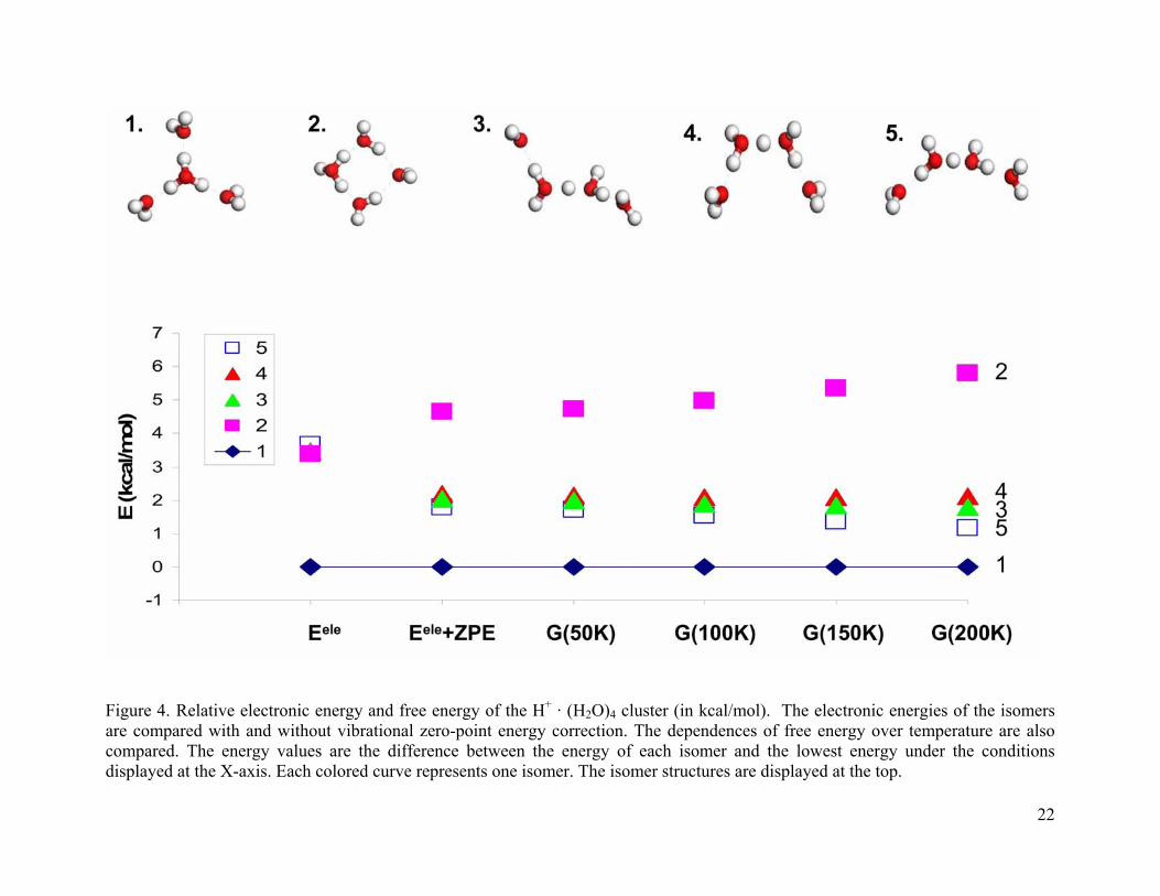
The structures and relative energies of five isomers of the (H2O)4 · H+ cluster are shown
in Figure 4. The relative energies are compared for a number of different situations. Eele is the
electronic energy of the B3LYP/6-31+G(d) optimized structure. Eele + ZPE includes both the
electronic energy and the vibrational zero-point energy correction. G(T) gives the free energy at
temperatures between 50 and 200 K. The isomers are numbered according to increasing
electronic energy.
Isomers 2-5 have very similar electronic energies. When zero-point energy is included,
the Zundel isomers 3-5 fall about 3 kcal/mol below isomer 2. The classic Eigen structure, isomer
1 remains the global minimum for all temperatures considered. Upon inclusion of the ZPE, the
four-membered ring structure (isomer 2) is the least stable isomer and becomes less stable as
temperature increases. Clearly, the Eigen structures (isomer 1 and 2) have larger zero-point
energy corrections than the Zundel structures (isomers 3-5).
For cluster size n = 4, the Eigen structure isomer 1 has a complete first solvation shell and
the proton charge is equally stabilized by three water molecules. The Zundel structures have only
a partial first solvation shell. It is not surprising that the Eigen structure is more stable than the
Zundel structures. The Eigen structure isomer 2 is not favored due to the strained four-membered
ring structure.
22
Figure 4. Relative electronic energy and free energy of the H+ · (H2O)4 cluster (in kcal/mol). The electronic energies of the isomers are compared with and without vibrational zero-point energy correction. The dependences of free energy over temperature are also compared. The energy values are the difference between the energy of each isomer and the lowest energy under the conditions displayed at the X-axis. Each colored curve represents one isomer. The isomer structures are displayed at the top.
23
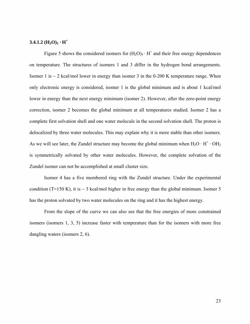
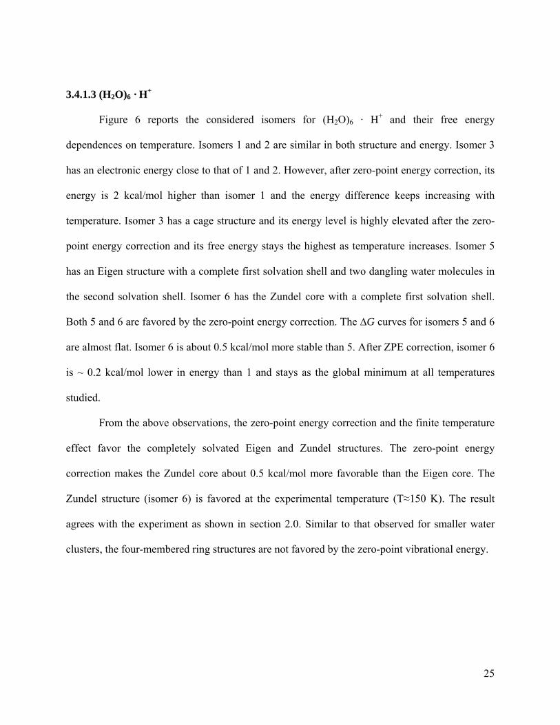
3.4.1.2 (H2O)5 · H+
Figure 5 shows the considered isomers for (H2O)5 · H+ and their free energy dependences
on temperature. The structures of isomers 1 and 3 differ in the hydrogen bond arrangements.
Isomer 1 is ~ 2 kcal/mol lower in energy than isomer 3 in the 0-200 K temperature range. When
only electronic energy is considered, isomer 1 is the global minimum and is about 1 kcal/mol
lower in energy than the next energy minimum (isomer 2). However, after the zero-point energy
correction, isomer 2 becomes the global minimum at all temperatures studied. Isomer 2 has a
complete first solvation shell and one water molecule in the second solvation shell. The proton is
delocalized by three water molecules. This may explain why it is more stable than other isomers.
As we will see later, the Zundel structure may become the global minimum when H2O · H+ · OH2
is symmetrically solvated by other water molecules. However, the complete solvation of the
Zundel isomer can not be accomplished at small cluster size.
Isomer 4 has a five membered ring with the Zundel structure. Under the experimental
condition (T≈150 K), it is ~ 3 kcal/mol higher in free energy than the global minimum. Isomer 5
has the proton solvated by two water molecules on the ring and it has the highest energy.
From the slope of the curve we can also see that the free energies of more constrained
isomers (isomers 1, 3, 5) increase faster with temperature than for the isomers with more free
dangling waters (isomers 2, 6).
24
Figure 5. Relative electronic energies and free energyies of typical H+ · (H2O)5 isomers (in kcal/mol). The electronic energies of the isomers are compared with and without vibrational zero-point energy correction. The dependences of free energy over temperature are also compared. The energy values are the difference between the energy of each isomer and the lowest energy under the conditions displayed at the X-axis. Each colored curve represents one isomer. The isomer structures are displayed at the top.
25
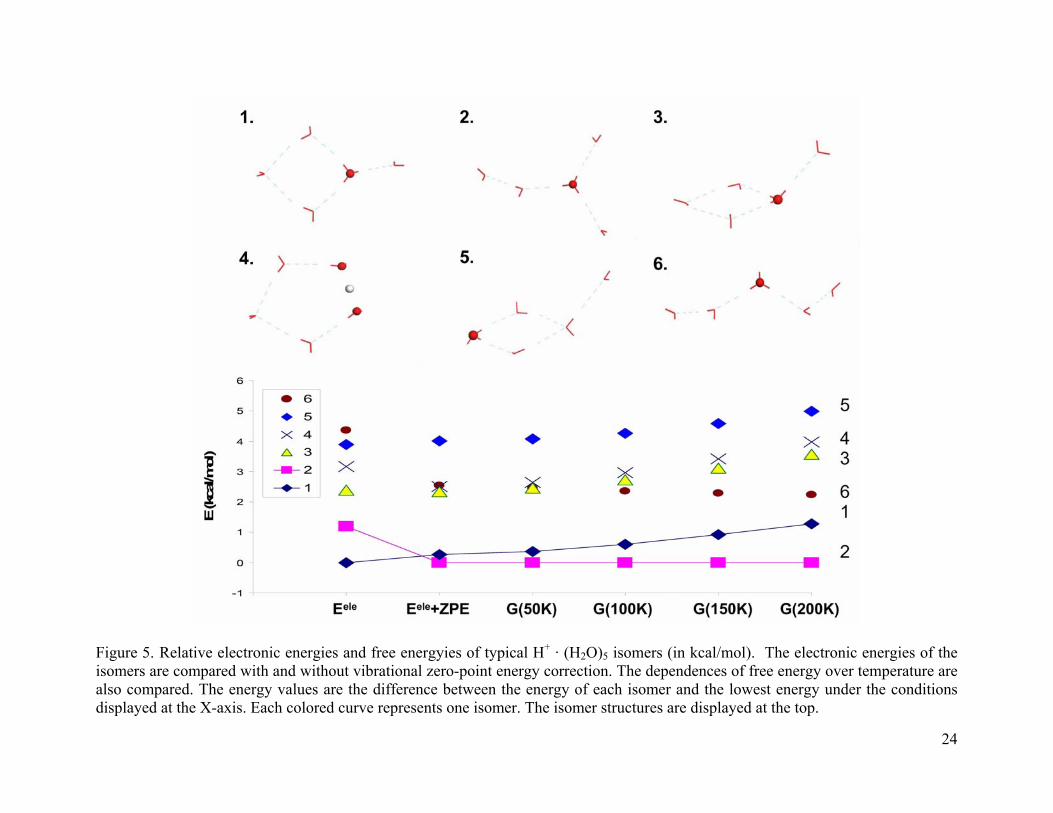
3.4.1.3 (H2O)6 · H+
Figure 6 reports the considered isomers for (H2O)6 · H+ and their free energy
dependences on temperature. Isomers 1 and 2 are similar in both structure and energy. Isomer 3
has an electronic energy close to that of 1 and 2. However, after zero-point energy correction, its
energy is 2 kcal/mol higher than isomer 1 and the energy difference keeps increasing with
temperature. Isomer 3 has a cage structure and its energy level is highly elevated after the zero-
point energy correction and its free energy stays the highest as temperature increases. Isomer 5
has an Eigen structure with a complete first solvation shell and two dangling water molecules in
the second solvation shell. Isomer 6 has the Zundel core with a complete first solvation shell.
Both 5 and 6 are favored by the zero-point energy correction. The ∆G curves for isomers 5 and 6
are almost flat. Isomer 6 is about 0.5 kcal/mol more stable than 5. After ZPE correction, isomer 6
is ~ 0.2 kcal/mol lower in energy than 1 and stays as the global minimum at all temperatures
studied.
From the above observations, the zero-point energy correction and the finite temperature
effect favor the completely solvated Eigen and Zundel structures. The zero-point energy
correction makes the Zundel core about 0.5 kcal/mol more favorable than the Eigen core. The
Zundel structure (isomer 6) is favored at the experimental temperature (T≈150 K). The result
agrees with the experiment as shown in section 2.0. Similar to that observed for smaller water
clusters, the four-membered ring structures are not favored by the zero-point vibrational energy.
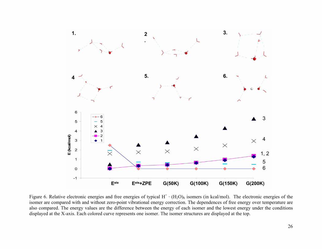
Figure 6. Relative electronic energies and free energies of typical H+ · (H2O)6 isomers (in kcal/mol). The electronic energies of the isomer are compared with and without zero-point vibrational energy correction. The dependences of free energy over temperature are also compared. The energy values are the difference between the energy of each isomer and the lowest energy under the conditions displayed at the X-axis. Each colored curve represents one isomer. The isomer structures are displayed at the top.
26
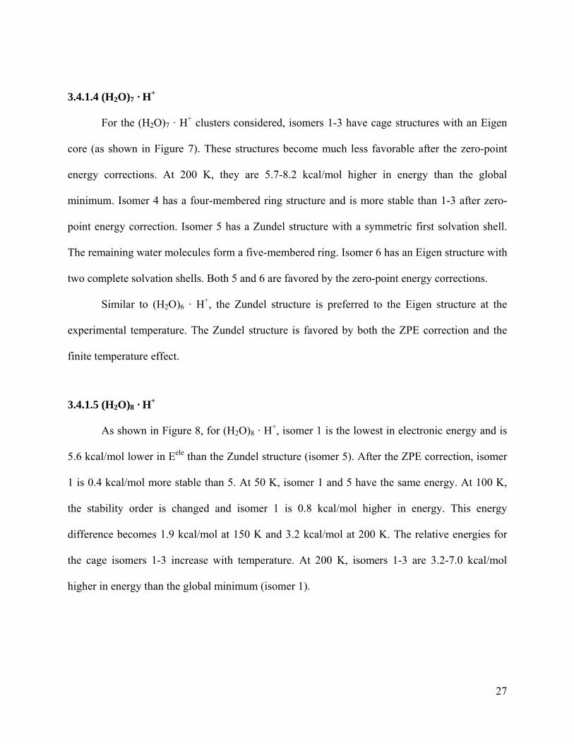
3.4.1.4 (H2O)7 · H+
For the (H2O)7 · H+ clusters considered, isomers 1-3 have cage structures with an Eigen
core (as shown in Figure 7). These structures become much less favorable after the zero-point
energy corrections. At 200 K, they are 5.7-8.2 kcal/mol higher in energy than the global
minimum. Isomer 4 has a four-membered ring structure and is more stable than 1-3 after zero-
point energy correction. Isomer 5 has a Zundel structure with a symmetric first solvation shell.
The remaining water molecules form a five-membered ring. Isomer 6 has an Eigen structure with
two complete solvation shells. Both 5 and 6 are favored by the zero-point energy corrections.
Similar to (H2O)6 · H+, the Zundel structure is preferred to the Eigen structure at the
experimental temperature. The Zundel structure is favored by both the ZPE correction and the
finite temperature effect.
3.4.1.5 (H2O)8 · H+
As shown in Figure 8, for (H2O)8 · H+, isomer 1 is the lowest in electronic energy and is
5.6 kcal/mol lower in Eele than the Zundel structure (isomer 5). After the ZPE correction, isomer
1 is 0.4 kcal/mol more stable than 5. At 50 K, isomer 1 and 5 have the same energy. At 100 K,
the stability order is changed and isomer 1 is 0.8 kcal/mol higher in energy. This energy
difference becomes 1.9 kcal/mol at 150 K and 3.2 kcal/mol at 200 K. The relative energies for
the cage isomers 1-3 increase with temperature. At 200 K, isomers 1-3 are 3.2-7.0 kcal/mol
higher in energy than the global minimum (isomer 1).
27
3.4.1.6 (H2O)n · H+, n = 9-12
Figure 9-Figure 12 summarize the relative stability of typical isomers of (H2O)n · H+, n =
9-12. For (H2O)9 · H+ isomers (as shown in Figure 9), the cage structures 1-4 are lower in
electronic energy. They become less favorable after ZPE correction and finite temperature
effects are considered. At 200 K, isomers 1-4 are 2.1-5.0 kcal/mol higher in energy than the
global minimum. Instead of the previous monotonous trends, the free energy of isomer 3 first
decreases, and then increases with the temperature. Isomer 1 is the global minimum up to 100 K.
However, in the temperature range of 100-200K, isomer 5 becomes the global minimum.
For the (H2O)10 · H+ cluster (as shown in Figure 10), isomer 1 is the lowest energy
structure at temperatures below 150 K. From 160 K - 200 K, isomer 4 becomes the global
minimum. The cage isomers 1-3 are 1.5-1.7 kcal/mol high in energy at 200 K. For the (H2O)10 ·
H+ cluster, isomer 2 and 4 are ~ 0.2 kcal/mol higher in energy than the global minimum around
150 K. For this small energy difference, it is possible than all three structures (isomers 1, 2, and
4) contribute in the experimental spectrum. We need to keep this in mind when make
conclusions during spectrum analysis. For (H2O)11 · H+ and (H2O)12 · H+ clusters (Figure 11 and
Figure 12), the cage structures dominate and no stable Zundel structures were found.
As the cluster size increases from n = 7 to 10, we can clearly see that cage isomers with
five-membered rings become more stable. At 200 K, their energies relative to the corresponding
global minimum are 5.7-8.2 kcal/mol (n = 7), 3.2-7.0 kcal/mol (n = 8), 2.1-5.0 kcal/mol (n = 9),
and 1.5-1.7 kcal/mol (n = 10), respectively. For cluster size n = 11 and 12, the cage isomers
dominate at all temperatures studied. At large cluster sizes, the cage structures are stabilized by a
large number of hydrogen bonds.
28
29
As the cluster size increases, the Zundel structure is only favored at high temperature. For
the (H2O)6 · H+ and (H2O)7 · H+ clusters, the Zundel structure is the global minimum at all
temperatures studied (0-200 K). For (H2O)8 · H+, the Zundel structure dominates after 50 K. This
change happens at 100 K for (H2O)9 · H+, and 150 K for (H2O)10 · H+. Although the zero-point
vibrational energy correction and finite temperature effect both favor the Zundel structure, cage
structures have much lower electronic energy than the Zundel structure. At low cluster size, the
finite temperature effect can overcome the electronic energy disadvantage for the Zundel
structure. As the cluster size increases, the electronic energy gap becomes larger and cannot be
compensated by an increase in temperature.
Figure 7. Relative electronic energies and free energies of typical H+ · (H2O)7 isomers (in kcal/mol). The electronic energies of the isomers are compared with and without zero-point vibrational energy correction. The dependences of free energy over temperature are also compared. The energy values are the difference between the energy of each isomer and the lowest energy under the conditions displayed at the X-axis. Each colored curve represents one isomer. The isomer structures are displayed at the top.
30
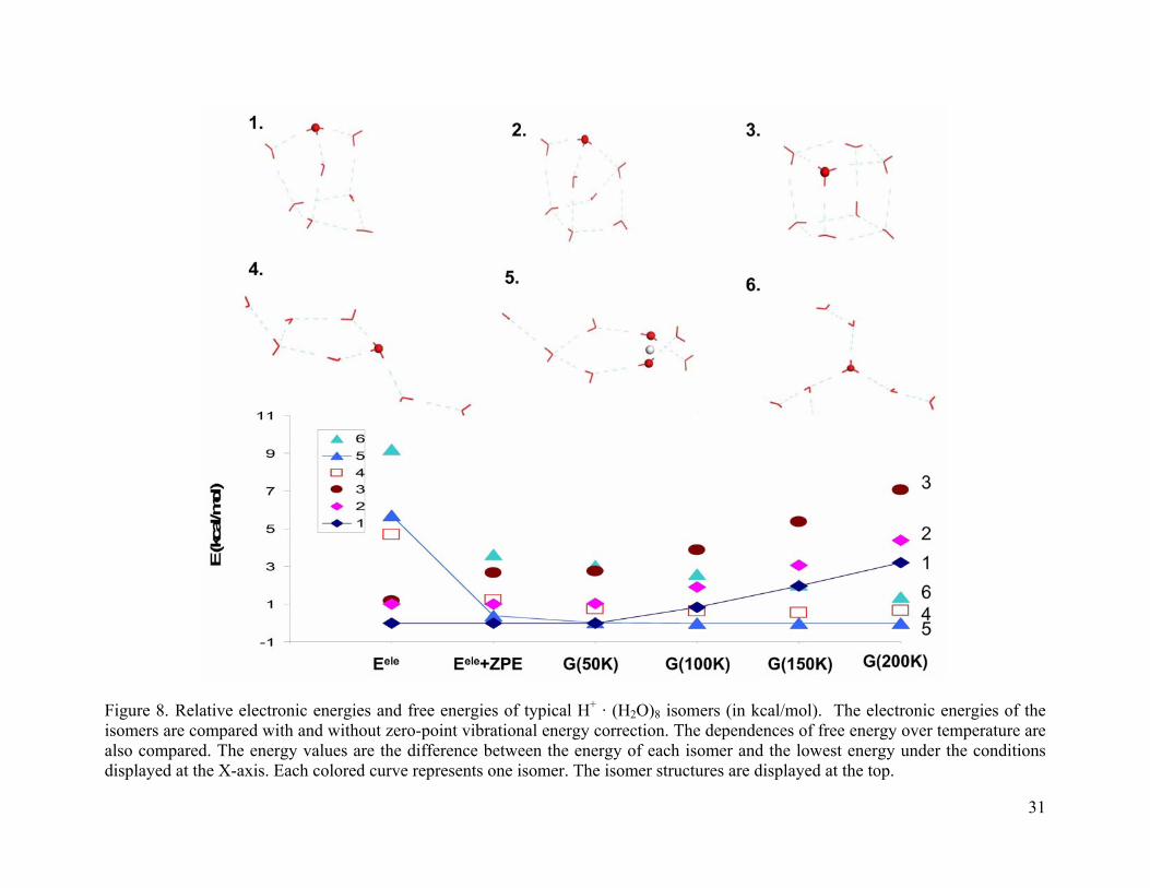
Figure 8. Relative electronic energies and free energies of typical H+ · (H2O)8 isomers (in kcal/mol). The electronic energies of the isomers are compared with and without zero-point vibrational energy correction. The dependences of free energy over temperature are also compared. The energy values are the difference between the energy of each isomer and the lowest energy under the conditions displayed at the X-axis. Each colored curve represents one isomer. The isomer structures are displayed at the top.
31
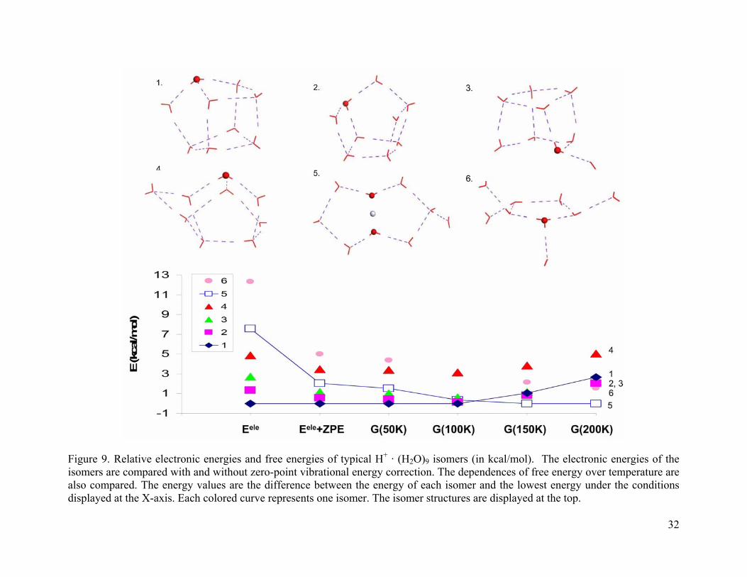
Figure 9. Relative electronic energies and free energies of typical H+ · (H2O)9 isomers (in kcal/mol). The electronic energies of the isomers are compared with and without zero-point vibrational energy correction. The dependences of free energy over temperature are also compared. The energy values are the difference between the energy of each isomer and the lowest energy under the conditions displayed at the X-axis. Each colored curve represents one isomer. The isomer structures are displayed at the top.
32
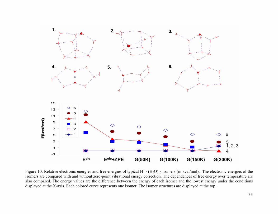
Figure 10. Relative electronic energies and free energies of typical H+ · (H2O)10 isomers (in kcal/mol). The electronic energies of the isomers are compared with and without zero-point vibrational energy correction. The dependences of free energy over temperature are also compared. The energy values are the difference between the energy of each isomer and the lowest energy under the conditions displayed at the X-axis. Each colored curve represents one isomer. The isomer structures are displayed at the top.
33
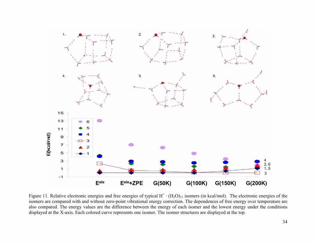
Figure 11. Relative electronic energies and free energies of typical H+ · (H2O)11 isomers (in kcal/mol). The electronic energies of the isomers are compared with and without zero-point vibrational energy correction. The dependences of free energy over temperature are also compared. The energy values are the difference between the energy of each isomer and the lowest energy under the conditions displayed at the X-axis. Each colored curve represents one isomer. The isomer structures are displayed at the top.
34
35
Figure 12. Relative electronic energies and free energies of typical H+ · (H2O)12 isomers (in kcal/mol). The electronic energies of the isomers are compared with and without zero-point vibrational energy correction. The dependences of free energy over temperature are also compared. The energy values are the difference between the energy of each isomer and the lowest energy under the conditions displayed at the X-axis. Each colored curve represents one isomer. The isomer structures are displayed at the top.
3.4.2 Effect of Ar tagging
Argon predissociation is an attractive methodology for the study of ion complexes. The
argon atoms cool down the protonated water clusters and act as “messengers” due to their low
detachment energy from the cluster. Much simpler spectrum can be obtained by attachment of
weakly bond Ar.27 However, the coexpansion with argon leads to mixed (H2O)n · H+ · Ar
clusters. It is unknown if the argon atoms change the chemical nature of the clusters we are
studying. The goal of this work is to develop a detailed understanding of how the Ar atoms
impact the structure and relative stability of cluster isomers. We will evaluate the extent of argon
perturbation on the intrinsic protonated water cluster structures through ab initio electronic
structure calculations and experimental spectroscopy for (H2O)n · H+ · Ar and (H2O)n · H+, n = 3-
8, clusters.
The perturbation by argon atoms on the H5O2+ Zundel structure26 has already been
studied.55 The narrow line widths and relative small (60 cm-1) perturbation introduced by the
addition of a second argon atom indicate that the basic “Zundel” character of the H5O2+ ion
survives upon complexation.64 In the following sections, we will study the perturbation by Ar
tagging to (H2O)n · H+ (n = 3-8) clusters.
36
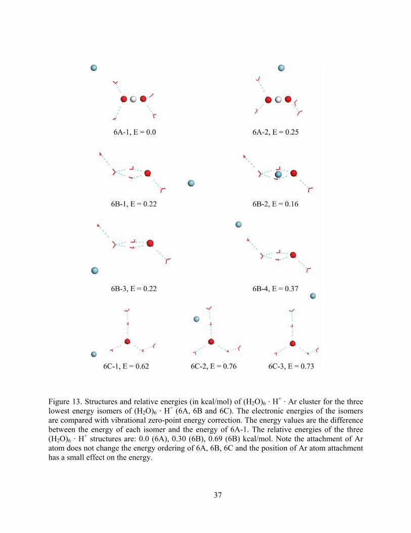
Figure 13. Structures and relative energies (in kcal/mol) of (H2O)6 · H+ · Ar cluster for the three lowest energy isomers of (H2O)6 · H+ (6A, 6B and 6C). The electronic energies of the isomers are compared with vibrational zero-point energy correction. The energy values are the difference between the energy of each isomer and the energy of 6A-1. The relative energies of the three (H2O)6 · H+ structures are: 0.0 (6A), 0.30 (6B), 0.69 (6B) kcal/mol. Note the attachment of Ar atom does not change the energy ordering of 6A, 6B, 6C and the position of Ar atom attachment has a small effect on the energy.
37
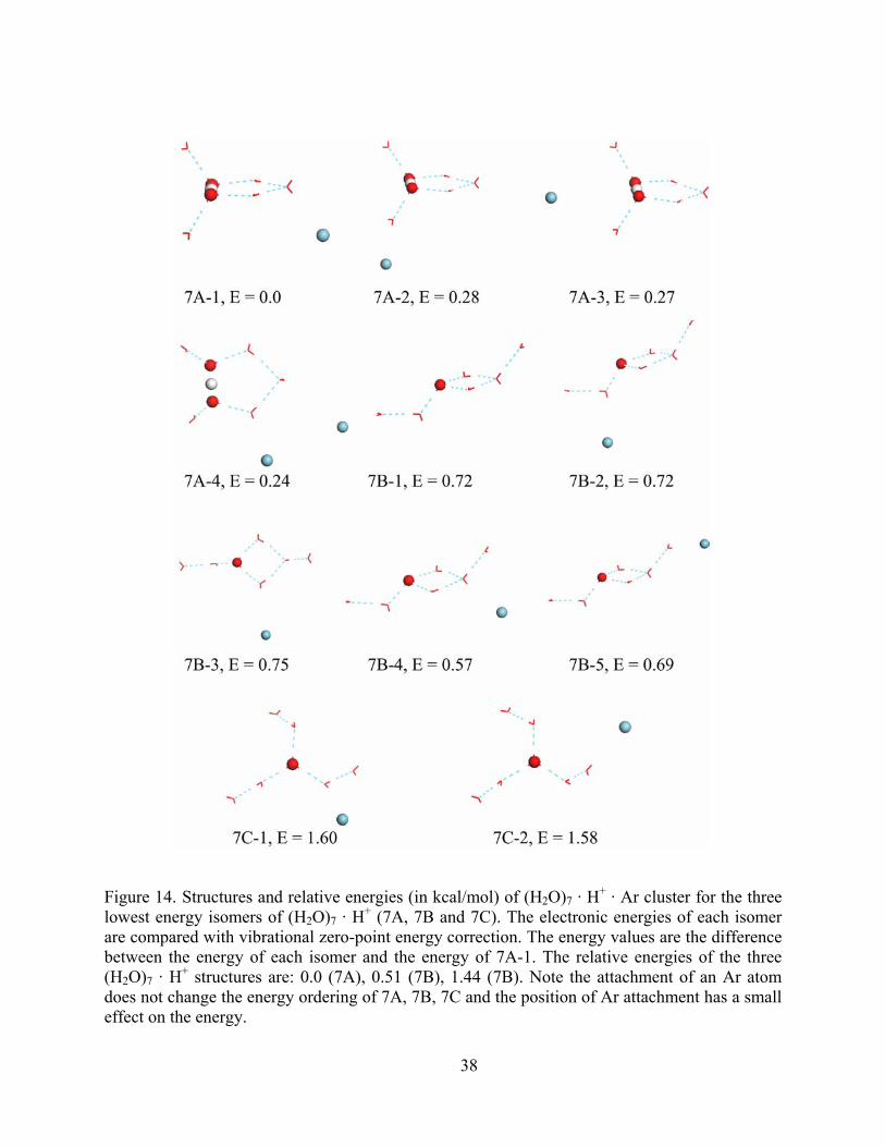
Figure 14. Structures and relative energies (in kcal/mol) of (H2O)7 · H+ · Ar cluster for the three lowest energy isomers of (H2O)7 · H+ (7A, 7B and 7C). The electronic energies of each isomer are compared with vibrational zero-point energy correction. The energy values are the difference between the energy of each isomer and the energy of 7A-1. The relative energies of the three (H2O)7 · H+ structures are: 0.0 (7A), 0.51 (7B), 1.44 (7B). Note the attachment of an Ar atom does not change the energy ordering of 7A, 7B, 7C and the position of Ar attachment has a small effect on the energy.
38
Several low energy structures for (H2O)n · H+ · Ar (n = 6-9) are chosen to study the
influence of the Ar atom complexation with the (H2O)n · H+ clusters. In Figure 13, we choose
three isomers 6A, 6B, and 6C of (H2O)6 · H+ cluster and calculate possible (H2O)n · H+ · Ar
minima and their relative energies. All the energies are corrected for ZPE and then compared
with the energy of 6A-1. Of these three structures, 6A is the global minimum of the (H2O)6 · H+
cluster, 6B and 6C are 0.30 and 0.69 kcal/mol higher in energy than 6A (after the ZPE
correction). The argon atom binds to a dangling hydrogen atom. In 6A-1, the Ar atom interacts
with a hydrogen atom of a water molecule in the first solvation shell. In 6A-2, the Ar atom stays
over the proton in a plane perpendicular to the H2O···H···OH2 axis. 6A-2 is 0.25 kcal/mol higher
in energy than 6A-1. 6B has four possible Ar complexes, their energy relative to 6A-1 are in the
range of 0.16-0.37 kcal/mol. The three possible Ar complexes for 6C have relative energies in
the range of 0.62-0.73 kcal/mol. The interaction with Ar atom at various positions causes an
energy span of 0.25 kcal/mol for 6A · Ar isomers, 0.21 kcal/mol for 6B · Ar isomers, and 0.11
kcal/mol for 6C · Ar isomers. Considering the relative energies of 6A, 6B and 6C (0.00, 0.30,
and 0.69 kcal/mol), we can see that the energy change upon binding of an Ar atom is small
compared to the energy difference of (H2O)6 · H+ isomers. The Ar attachment does not change
the energy ordering in all three cases.
Figure 14 shows the corresponding results for the isomers 7A, AB and 7C of the (H2O)7 ·
H+ cluster. The energies of 7B and 7C relative to 7A are 0.51 kcal/mol and 1.44 kcal/mol,
respectively. The four possible (H2O)7 · H+ · Ar isomers of 7A differ in energy by less than 0.28
kcal/mol. The Ar complexes have a relative energy range of 0.57-0.75 kcal/mol for 7B · Ar, and
1.58-1.60 kcal/mol for 7C · Ar. In total, Ar attaching causes the relative energy to change by up
to 0.28 kcal/mol, which is small compared to the energy differences between 7A, 7B and 7C.
39
From Figure 13 and Figure 14, we can see that the ordering of the low energy isomers of
the (H2O)n · H+ cluster does not change upon Ar tagging.
Next, we will compare the experimental spectra of (H2O)n · H+ and (H2O)n · H+ · Ar
clusters (n = 3-8). Figure 15 and Figure 16 exhibit the predissociation spectra for (H2O)n · H+ and
(H2O)n · H+ · Ar (n = 3-8) clusters side by side in the 2000-4000 cm-1 wavelength range. Both
figures show that the spectra of (H2O)n · H+ · Ar clusters have higher resolution than the (H2O)n ·
H+ spectra. To produce the predissociation spectrum of (H2O)n · H+, the cluster needs to
photodetach one water molecule. In the (H2O)n · H+ · Ar case, the cluster photodetaches an Ar
atom. Simulations of the (H2O)4 · H+ global minimum structure with MP2/aug-cc-pVDZ method
gives 1.45 kcal/mol for the Ar detaching from a dangling water molecule, 1.78 kcal/mol for the
Ar detaching from a position over the proton, and 13.71 kcal/mol for a water molecule
dissociation. The low Ar dissociation energy leads to cooler (H2O)n · H+ clusters and thus higher
resolution predissociation spectra.
In Figure 15, the (H2O)3 · H+, and (H2O)5 · H+ clusters have similar spectra with and
without Ar tagging. No obvious peak shifts are observed upon Ar complexation. For the (H2O)4 ·
H+ cluster, the spectrum after Ar tagging has a broad peak at 2665 cm-1. This comes from the
degenerate asymmetric OH stretching vibration in an intact Eigen core.65 Due to the high
dissociation energy of water, the 2665 cm-1 peak becomes invisible for the (H2O)4 · H+ cluster
spectrum without Ar tagging.
Because of the high energy needed to detach H2O from the second solvation shell, it is
possible that multiple isomers contribute to the spectrum for bare clusters. The experimental
spectra for (H2O)6 · H+ and (H2O)7 · H+ clearly show the existence of more than one structure.
The bare six-membered cluster has peaks at ~ 3000 cm-1 and ~ 3320 cm-1, which can attribute to
40
the Eigen structure shown in Figure 6 (5). There are notable differences between the bare and
Ar-tagged (H2O)7 · H+ clusters in the 3100-3600 cm-1 range, which may come from structures 4
and 6 in Figure 7. The (H2O)8 · H+ spectrum appears quite similar for both the bare and the Ar-
tagged species.
The Ar tagging does not give obvious shifts to the frequencies. However, some
discrepancies between the spectra with and without Ar tagging are expected due to the
dissociation energy difference between Ar and H2O.
41
2000 2200 2400 2600 2800 3000 3200 3400 3600 3800 4000
H+(H2O)3Ar
H+(H2O)5
H+(H2O)5Ar
H+(H2O)4
H+(H2O)4Ar
H+(H2O)3
Figure 15. Comparison of predissociation spectra of H+ · (H2O)n, n = 3 – 5 with and without Ar tagging, with n increasing from bottom to top. (Spectra provided by Prof. M. Duncan)
42
2000 2200 2400 2600 2800 3000 3200 3400 3600 3800 4000
H+(H2O)6Ar
H+(H2O)8
H+(H2O)8Ar
H+(H2O)7
H+(H2O)7Ar
H+(H2O)6
Figure 16. Comparison of predissociation spectra of H+ · (H2O)n, n = 6 – 8 with and without argon, with n increasing from bottom to top. (Spectra provided by Prof. M. Duncan)
43
3.5 CONCLUSIONS
The relative stability of various isomers of (H2O)n · H+, n = 4-12, have been studied with
density functional theory. The influence of vibrational zero-point energy correction and finite
temperature effects are considered. It was found that both the vibrational zero-point energy
correction and finite temperature effect impact the relative stability of the isomers and favor the
Zundel ion with symmetric solvation shells. As cluster size increases, the caged structures
compete with the Zundel structures and gradually dominate the population.
The perturbation of Ar atoms on Ar-tagged and non-tagged spectra of (H2O)n · H+, n = 3-
8, has also been studied with both density functional theory and predissociation spectroscopy.
Optimization with B3LYP/6-31+G(d) method reveals that Ar tagging does not change the energy
ordering of the (H2O)n · H+, n = 6-8, isomers. The experimental spectra with and without Ar
tagging indicate that the Ar atom helps to achieve high resolution spectra and has little effect on
the frequencies.
3.6 ACKNOWLEDGEMENTS
This research was carried out with the support of the National Science Foundation (Grant
No. CHE-0244143, 0111245, and 0078528). The calculations were carried out on computers in
the University of Pittsburgh’s Center for Molecular and Materials Simulations.
44
4.0 THEORETICAL CHARACTERIZATION OF THE (H2O)21 CLUSTER:
APPLICATION OF AN N-BODY DECOMPOSITION PROCEDURE
This work was published as:
Cui J., Liu H., Jordan K.D., J. Phys. Chem. B 110(38) 18872-18878 (2006).66
4.1 ABSTRACT
Two low-energy minima of (H2O)21 with very different H-bonding arrangements have been
investigated with the B3LYP density functional and RIMP2 methods, as well as with the TIP4P,
Dang–Chang, AMOEBA, and TTM2-F force fields. The AMOEBA and TTM2-F model
potentials give an energy ordering that agrees with the results of the electronic structure
calculations, while the TIP4P and Dang–Chang models give the opposite ordering. Insight into
the role of many-body polarization for establishing the relative stability of the two isomers is
provided by an n-body decomposition of the energies calculated using the various theoretical
methods.
45
4.2 INTRODUCTION
Over the past few years, major strides have been made in understanding the structure and
dynamics of water clusters. Recently, there has been renewed interest in the H+(H2O)21
cluster,16,36,67-69 which appears as a magic number in the mass spectra of H+(H2O)n clusters.28,70-72
Over three decades ago, Searcy and Fenn proposed that the n = 21 protonated cluster has a
structure corresponding to a water dodecahedron with an enclosed water monomer and the
excess proton on the surface.28 Wei and Castleman, on the basis of a titration experiment, offered
an alternative interpretation, namely, that the H+(H2O)21 cluster is comprised of a water
dodecahedron with an interior H3O+ ion.70 Comparison of the measured vibrational
predissociation spectrum16,36 with the calculated harmonic vibrational spectra of various isomers
leads to the conclusion that the experimentally observed isomer is that originally proposed by
Searcy and Fenn with the excess proton on the surface of the cluster.16,36,67 Moreover, the
calculations indicate that the Searcy–Fenn isomer is the global minimum of H+(H2O)21.16,68,69
Subsequent molecular dynamics simulations confirm this picture, but indicate that, as a result of
the finite temperature of the cluster, isomers other than the global minimum also contribute to the
observed spectrum.73
For the neutral (H2O)20 cluster, the most stable dodecahedral isomer lies about 10 kcal/mol
above the global minimum isomer which has a pentagonal prism (PP) structure.74,75 This would
seem to suggest that the presence of the proton is the key to the high stability of the
dodecahedrally derived global minimum isomer of H+(H2O)21. However, Lee and Beauchamp
have observed a magic number at n = 21 for [tetrabutylammonium + (H2O)n]+ clusters,76 and
since the charge in this mixed cluster is associated with the amine, this suggests that the water
46
molecules are present as an (H2O)21 cluster with especially high stability. Although H+(H2O)21
and (H2O)20 have been the subject of numerous theoretical studies, the neutral (H2O)21 cluster
has received much less attention. Wales and Hodges have characterized (H2O)21 using the TIP4P
water model77 and reported that the global minimum has a “flat” structure comprised of fused
four- and five-membered rings,74 and hereafter referred to as TIP4P-gm(21). More recently,
Hartke78 showed, using the polarizable TTM2-F79 model potential, that there is a lower energy
isomer based on the (H2O)20 water dodecahedron with an interior water molecule engaged in four
H-bonds. We refer to this species as DD*(20,1), where the “DD” denotes distorted
dodecahedron, and the numbers in parentheses indicate that there is one water monomer inside
the (H2O)20 dodecahedral cage. The asterisk is to distinguish this isomer from the closely related
DD(20,1) isomer considered in the present work, and which lies only 0.6 kcal/mol above the
DD*(20,1) isomer. These two isomers can be interconverted by six donor–acceptor exchanges of
the H-bonding network of the water molecules on the surface of the cluster.
In this paper, we present a detailed theoretical study of the TIP4P-gm(21) and DD(20,1)
isomers of (H2O)21, with an emphasis on elucidating the level of theory needed to describe the
relative stability of the two isomers. Results are reported for the B3LYP density functional80-82
and the resolvent-of-the-identity second-order Møller–Plesset perturbation theory (RIMP2)83,84
electronic structure methods, as well as for the TIP4P77 effective 2-body model potential and for
the Dang–Chang (DC),85 Amoeba,86 and TTM2-F79 polarizable water models.
We also report the 1-, 2-, 3-, and 4-body contributions,87 1EΔ , 2EΔ , , and 3EΔ 4EΔ ,
respectively, to the net interaction energies. These are defined as
47
∑ ∑ ∑ ∑
∑ ∑ ∑
∑ ∑
∑
−
=
−
+=
−
+= +=
−
=
−
+= +=
−
= +=
=
−−−−++++++−−−−
=Δ
+++−−−=Δ
−−=Δ
⋅−=Δ
3
1
2
1
1
1 14
2
1
1
1 13
1
1 12
11
)]()()()(),(),(),(),(),(),(
),,(),,(),,(),,(),,,([
)]()()(),(),(),(),,([
)]()(),([
)(
N
i
N
ij
N
jk
N
kl
N
i
N
ij
N
jk
N
i
N
ij
N
iw
lEkEjEiElkEljEkjEliEkiEjiE
lkjElkiEljiEkjiElkjiEE
kEjEiEkjEkiEjiEkjiEE
jEiEjiEE
EniEE
where E(i), E(i,j), E(i,j,k), and E(i,j,k,l) are, respectively, the energies of the monomer i, dimer
(i,j), trimer (i,j,k) and tetramer (i,j,k,l) cut out of the full cluster, and Ew is the energy of the
monomer at its optimized geometry. 1EΔ , thus, gives the relaxation energy associated with the
distortion of the monomers in going from the gas phase to the cluster. For the rigid monomer
TIP4P and DC models, is zero. 1EΔ
There is a twofold motivation for examining the individual n-body contributions. First, the
decomposition of the interaction energies into their n-body components provides additional
insight into the importance of various terms in the intermolecular potential for determining the
relative stability of different isomers. Second, (H2O)21 is an excellent test case for the n-body
decomposition method for calculating MP2-level interaction energies.19 This method exploits the
rapid convergence of the n-body expansion of the interaction energy of water cluster,17,88
approximating the total interaction (binding) energy as 321 EEEE Δ+Δ+Δ≈Δ or
. 4321 EEEEE Δ+Δ+Δ+Δ≈Δ
To date, the largest cluster to which this approach has been applied using MP2-level
interaction energies is the hexamer.19 By applying it to a cluster containing 21 water molecules,
we can explore the viability of distance-dependent screening strategies for identifying 3- and 4-
48
body terms that can be neglected, thereby reducing the computational costs. Examination of the
n-body contributions also provides new insights into the suitability of density functional methods
and of various model potentials for describing the relative stabilities of different isomers of water
clusters.
4.3 COMPUTATIONAL DETAILS
The geometries of the two (H2O)21 isomers and of three forms of (H2O)20 included for
comparison and described below were optimized using each of the theoretical methods
considered. The geometry optimizations with the B3LYP and RIMP2 procedures were
performed using the aug-cc-pVDZ basis sets.89,90 These were followed by single–point
calculations using the more flexible aug-cc-pVTZ(-f) basis set, where the –f indicates that the f
functions on the O atoms and the d functions on the H atoms that would be present in the full
aug-cc-pVTZ basis set have been omitted. The B3LYP and RIMP2 calculations were carried out
using Gaussian 0359 and Turbomole,91,92 respectively. The calculations with the TIP4P, DC, and
AMOEBA force fields were carried out using the Tinker program,86,93-95 and the calculations
with the TTM2-F force field were carried out using the Occident program.79
The DC model is a rigid monomer model, using three point charges to represent the
electrostatics, a single isotropic polarizable site, and OO Lennard-Jones interactions. This model
places positive point charges on each H atom and the balancing negative point charge on the so-
called M site, which is located on the rotational axis, displaced 0.215 Å from the O atom toward
the H atoms. The isotropic polarizable center is also located at the M site.
49
The TTM2-F and AMOEBA models employ flexible monomers and three atom-centered,
mutually interacting, polarizable sites. The TTM2-F model, like the DC model, represents the
charge distribution by three point charges (with the positive charges on the H atoms and the
negative charge on the M site), whereas the AMOEBA model employs distributed multipoles
through quadrupoles on the three atoms. The TTM2-F model uses R-12, R-10, and R-6 terms
between the O atoms to represent the dispersion interactions and short-range repulsion, while the
AMOEBA model employs buffered 7–14 OO, HH, and HO potentials to represent these
interactions. Both the AMOEBA and TTM2-F models use a Thole-type damping96 of the
charge–induced dipole interactions and also of the induced dipole–induced dipole interactions.
The TTM2-F model damps the charge–charge interactions as well. All three of these polarizable
models give values of the dipole and quadrupole moments of the water monomer close to the
corresponding experimental values and have been applied with considerable success to water
clusters as well as to bulk water.79,85,86,93
The two low-energy isomers of (H2O)21 considered in this work are shown in Figure 17. As
noted above, these are the global minimum located with the TIP4P model potential and
designated TIP4P-gm(21) and an isomer designated DD(20,1) to indicate that it can be viewed as
a distorted dodecahedron with an interior water molecule.
To aid in analyzing the results for (H2O)21, we also considered the four structures for (H2O)20
shown in Figure 17. These include the “perfect” dodecahedron [PD(20)], the pentagonal prism
[PP(20)], the DD(19,1) isomer, which is formed by removing a water from the surface of
DD(20,1) and allowing for geometrical relaxation, and a structure designated DD(20,0), formed
by removing the interior water molecule from DD(20,1), without allowing relaxation of the
geometry.
50
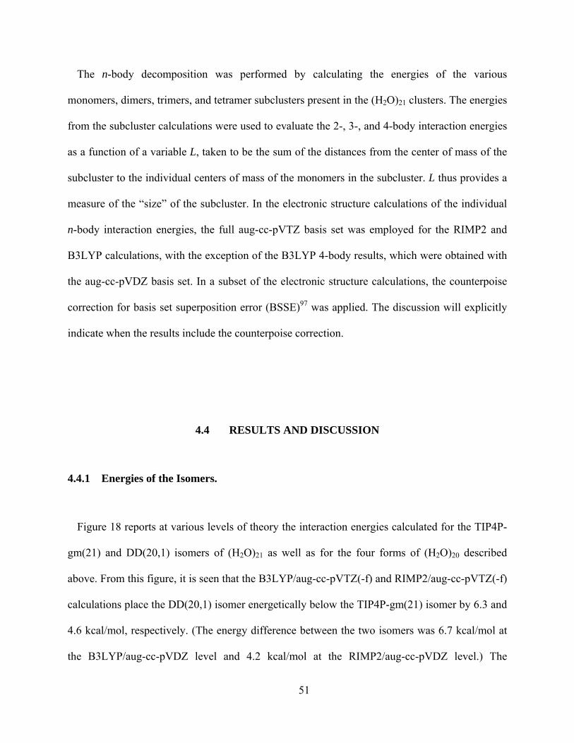
The n-body decomposition was performed by calculating the energies of the various
monomers, dimers, trimers, and tetramer subclusters present in the (H2O)21 clusters. The energies
from the subcluster calculations were used to evaluate the 2-, 3-, and 4-body interaction energies
as a function of a variable L, taken to be the sum of the distances from the center of mass of the
subcluster to the individual centers of mass of the monomers in the subcluster. L thus provides a
measure of the “size” of the subcluster. In the electronic structure calculations of the individual
n-body interaction energies, the full aug-cc-pVTZ basis set was employed for the RIMP2 and
B3LYP calculations, with the exception of the B3LYP 4-body results, which were obtained with
the aug-cc-pVDZ basis set. In a subset of the electronic structure calculations, the counterpoise
correction for basis set superposition error (BSSE)97 was applied. The discussion will explicitly
indicate when the results include the counterpoise correction.
4.4 RESULTS AND DISCUSSION
4.4.1 Energies of the Isomers.
Figure 18 reports at various levels of theory the interaction energies calculated for the TIP4P-
gm(21) and DD(20,1) isomers of (H2O)21 as well as for the four forms of (H2O)20 described
above. From this figure, it is seen that the B3LYP/aug-cc-pVTZ(-f) and RIMP2/aug-cc-pVTZ(-f)
calculations place the DD(20,1) isomer energetically below the TIP4P-gm(21) isomer by 6.3 and
4.6 kcal/mol, respectively. (The energy difference between the two isomers was 6.7 kcal/mol at
the B3LYP/aug-cc-pVDZ level and 4.2 kcal/mol at the RIMP2/aug-cc-pVDZ level.) The
51
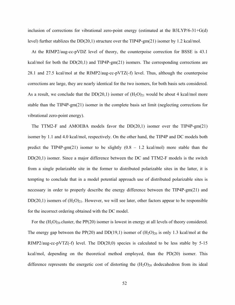
inclusion of corrections for vibrational zero-point energy (estimated at the B3LYP/6-31+G(d)
level) further stablizes the DD(20,1) structure over the TIP4P-gm(21) isomer by 1.2 kcal/mol.
At the RIMP2/aug-cc-pVDZ level of theory, the counterpoise correction for BSSE is 43.1
kcal/mol for both the DD(20,1) and TIP4P-gm(21) isomers. The corresponding corrections are
28.1 and 27.5 kcal/mol at the RIMP2/aug-cc-pVTZ(-f) level. Thus, although the counterpoise
corrections are large, they are nearly identical for the two isomers, for both basis sets considered.
As a result, we conclude that the DD(20,1) isomer of (H2O)21 would be about 4 kcal/mol more
stable than the TIP4P-gm(21) isomer in the complete basis set limit (neglecting corrections for
vibrational zero-point energy).
The TTM2-F and AMOEBA models favor the DD(20,1) isomer over the TIP4P-gm(21)
isomer by 1.1 and 4.0 kcal/mol, respectively. On the other hand, the TIP4P and DC models both
predict the TIP4P-gm(21) isomer to be slightly (0.8 – 1.2 kcal/mol) more stable than the
DD(20,1) isomer. Since a major difference between the DC and TTM2-F models is the switch
from a single polarizable site in the former to distributed polarizable sites in the latter, it is
tempting to conclude that in a model potential approach use of distributed polarizable sites is
necessary in order to properly describe the energy difference between the TIP4P-gm(21) and
DD(20,1) isomers of (H2O)21. However, we will see later, other factors appear to be responsible
for the incorrect ordering obtained with the DC model.
For the (H2O)20 cluster, the PP(20) isomer is lowest in energy at all levels of theory considered.
The energy gap between the PP(20) and DD(19,1) isomer of (H2O)20 is only 1.3 kcal/mol at the
RIMP2/aug-cc-pVTZ(-f) level. The DD(20,0) species is calculated to be less stable by 5-15
kcal/mol, depending on the theoretical method employed, than the PD(20) isomer. This
difference represents the energetic cost of distorting the (H2O)20 dodecahedron from its ideal
52
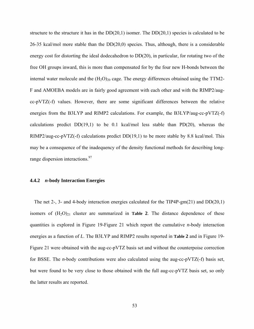
structure to the structure it has in the DD(20,1) isomer. The DD(20,1) species is calculated to be
26-35 kcal/mol more stable than the DD(20,0) species. Thus, although, there is a considerable
energy cost for distorting the ideal dodecahedron to DD(20), in particular, for rotating two of the
free OH groups inward, this is more than compensated for by the four new H-bonds between the
internal water molecule and the (H2O)20 cage. The energy differences obtained using the TTM2-
F and AMOEBA models are in fairly good agreement with each other and with the RIMP2/aug-
cc-pVTZ(-f) values. However, there are some significant differences between the relative
energies from the B3LYP and RIMP2 calculations. For example, the B3LYP/aug-cc-pVTZ(-f)
calculations predict DD(19,1) to be 0.1 kcal/mol less stable than PD(20), whereas the
RIMP2/aug-cc-pVTZ(-f) calculations predict DD(19,1) to be more stable by 8.8 kcal/mol. This
may be a consequence of the inadequency of the density functional methods for describing long-
range dispersion interactions.97
4.4.2 n-body Interaction Energies
The net 2-, 3- and 4-body interaction energies calculated for the TIP4P-gm(21) and DD(20,1)
isomers of (H2O)21 cluster are summarized in Table 2. The distance dependence of these
quantities is explored in Figure 19-Figure 21 which report the cumulative n-body interaction
energies as a function of L. The B3LYP and RIMP2 results reported in Table 2 and in Figure 19-
Figure 21 were obtained with the aug-cc-pVTZ basis set and without the counterpoise correction
for BSSE. The n-body contributions were also calculated using the aug-cc-pVTZ(-f) basis set,
but were found to be very close to those obtained with the full aug-cc-pVTZ basis set, so only
the latter results are reported.
53
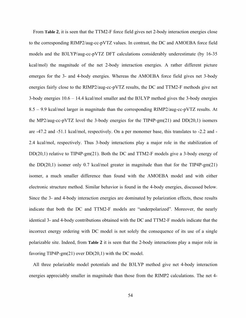
From Table 2, it is seen that the TTM2-F force field gives net 2-body interaction energies close
to the corresponding RIMP2/aug-cc-pVTZ values. In contrast, the DC and AMOEBA force field
models and the B3LYP/aug-cc-pVTZ DFT calculations considerably underestimate (by 16-35
kcal/mol) the magnitude of the net 2-body interaction energies. A rather different picture
emerges for the 3- and 4-body energies. Whereas the AMOEBA force field gives net 3-body
energies fairly close to the RIMP2/aug-cc-pVTZ results, the DC and TTM2-F methods give net
3-body energies 10.6 – 14.4 kcal/mol smaller and the B3LYP method gives the 3-body energies
8.5 – 9.9 kcal/mol larger in magnitude than the corresponding RIMP2/aug-cc-pVTZ results. At
the MP2/aug-cc-pVTZ level the 3-body energies for the TIP4P-gm(21) and DD(20,1) isomers
are -47.2 and -51.1 kcal/mol, respectively. On a per monomer base, this translates to -2.2 and -
2.4 kcal/mol, respectively. Thus 3-body interactions play a major role in the stabilization of
DD(20,1) relative to TIP4P-gm(21). Both the DC and TTM2-F models give a 3-body energy of
the DD(20,1) isomer only 0.7 kcal/mol greater in magnitude than that for the TIP4P-gm(21)
isomer, a much smaller difference than found with the AMOEBA model and with either
electronic structure method. Similar behavior is found in the 4-body energies, discussed below.
Since the 3- and 4-body interaction energies are dominated by polarization effects, these results
indicate that both the DC and TTM2-F models are “underpolarized”. Moreover, the nearly
identical 3- and 4-body contributions obtained with the DC and TTM2-F models indicate that the
incorrect energy ordering with DC model is not solely the consequence of its use of a single
polarizable site. Indeed, from Table 2 it is seen that the 2-body interactions play a major role in
favoring TIP4P-gm(21) over DD(20,1) with the DC model.
All three polarizable model potentials and the B3LYP method give net 4-body interaction
energies appreciably smaller in magnitude than those from the RIMP2 calculations. The net 4-
54
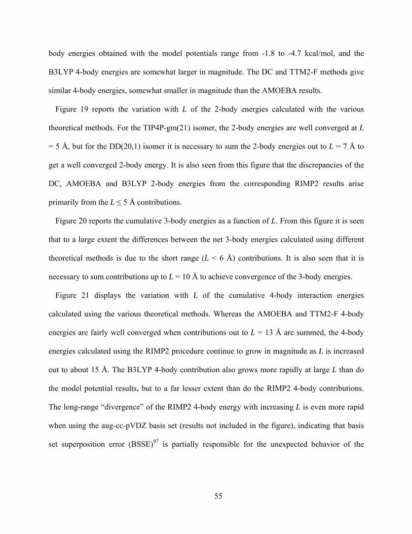
body energies obtained with the model potentials range from -1.8 to -4.7 kcal/mol, and the
B3LYP 4-body energies are somewhat larger in magnitude. The DC and TTM2-F methods give
similar 4-body energies, somewhat smaller in magnitude than the AMOEBA results.
Figure 19 reports the variation with L of the 2-body energies calculated with the various
theoretical methods. For the TIP4P-gm(21) isomer, the 2-body energies are well converged at L
= 5 Å, but for the DD(20,1) isomer it is necessary to sum the 2-body energies out to L = 7 Å to
get a well converged 2-body energy. It is also seen from this figure that the discrepancies of the
DC, AMOEBA and B3LYP 2-body energies from the corresponding RIMP2 results arise
primarily from the L ≤ 5 Å contributions.
Figure 20 reports the cumulative 3-body energies as a function of L. From this figure it is seen
that to a large extent the differences between the net 3-body energies calculated using different
theoretical methods is due to the short range (L < 6 Å) contributions. It is also seen that it is
necessary to sum contributions up to L = 10 Å to achieve convergence of the 3-body energies.
Figure 21 displays the variation with L of the cumulative 4-body interaction energies
calculated using the various theoretical methods. Whereas the AMOEBA and TTM2-F 4-body
energies are fairly well converged when contributions out to L = 13 Å are summed, the 4-body
energies calculated using the RIMP2 procedure continue to grow in magnitude as L is increased
out to about 15 Å. The B3LYP 4-body contribution also grows more rapidly at large L than do
the model potential results, but to a far lesser extent than do the RIMP2 4-body contributions.
The long-range “divergence” of the RIMP2 4-body energy with increasing L is even more rapid
when using the aug-cc-pVDZ basis set (results not included in the figure), indicating that basis
set superposition error (BSSE)97 is partially responsible for the unexpected behavior of the
55
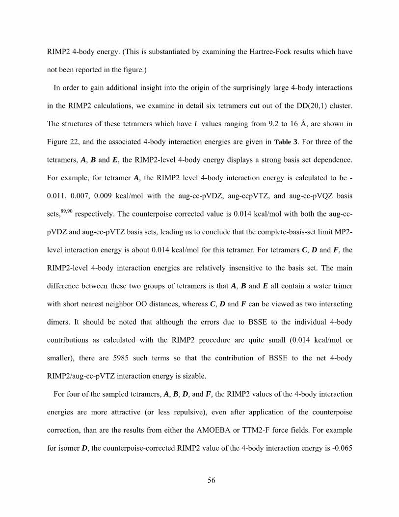
RIMP2 4-body energy. (This is substantiated by examining the Hartree-Fock results which have
not been reported in the figure.)
In order to gain additional insight into the origin of the surprisingly large 4-body interactions
in the RIMP2 calculations, we examine in detail six tetramers cut out of the DD(20,1) cluster.
The structures of these tetramers which have L values ranging from 9.2 to 16 Å, are shown in
Figure 22, and the associated 4-body interaction energies are given in Table 3. For three of the
tetramers, A, B and E, the RIMP2-level 4-body energy displays a strong basis set dependence.
For example, for tetramer A, the RIMP2 level 4-body interaction energy is calculated to be -
0.011, 0.007, 0.009 kcal/mol with the aug-cc-pVDZ, aug-ccpVTZ, and aug-cc-pVQZ basis
sets,89,90 respectively. The counterpoise corrected value is 0.014 kcal/mol with both the aug-cc-
pVDZ and aug-cc-pVTZ basis sets, leading us to conclude that the complete-basis-set limit MP2-
level interaction energy is about 0.014 kcal/mol for this tetramer. For tetramers C, D and F, the
RIMP2-level 4-body interaction energies are relatively insensitive to the basis set. The main
difference between these two groups of tetramers is that A, B and E all contain a water trimer
with short nearest neighbor OO distances, whereas C, D and F can be viewed as two interacting
dimers. It should be noted that although the errors due to BSSE to the individual 4-body
contributions as calculated with the RIMP2 procedure are quite small (0.014 kcal/mol or
smaller), there are 5985 such terms so that the contribution of BSSE to the net 4-body
RIMP2/aug-cc-pVTZ interaction energy is sizable.
For four of the sampled tetramers, A, B, D, and F, the RIMP2 values of the 4-body interaction
energies are more attractive (or less repulsive), even after application of the counterpoise
correction, than are the results from either the AMOEBA or TTM2-F force fields. For example
for isomer D, the counterpoise-corrected RIMP2 value of the 4-body interaction energy is -0.065
56
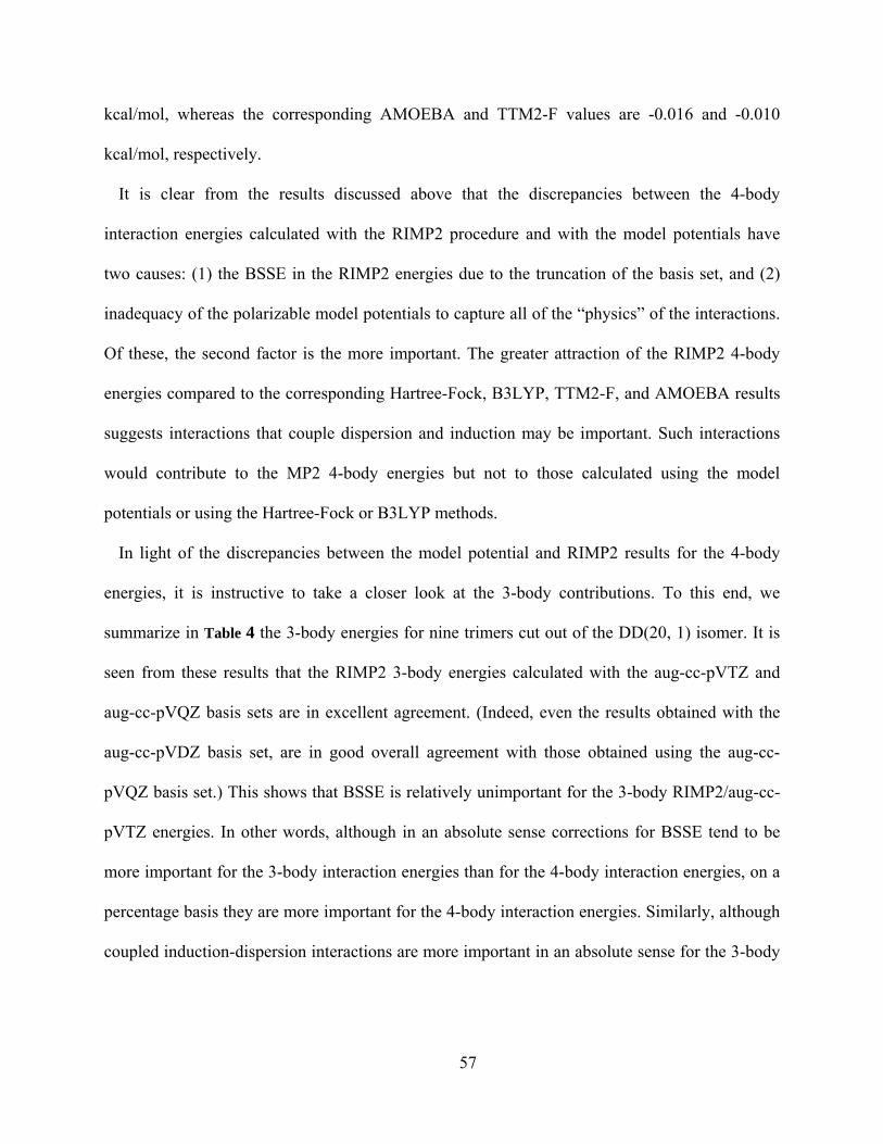
kcal/mol, whereas the corresponding AMOEBA and TTM2-F values are -0.016 and -0.010
kcal/mol, respectively.
It is clear from the results discussed above that the discrepancies between the 4-body
interaction energies calculated with the RIMP2 procedure and with the model potentials have
two causes: (1) the BSSE in the RIMP2 energies due to the truncation of the basis set, and (2)
inadequacy of the polarizable model potentials to capture all of the “physics” of the interactions.
Of these, the second factor is the more important. The greater attraction of the RIMP2 4-body
energies compared to the corresponding Hartree-Fock, B3LYP, TTM2-F, and AMOEBA results
suggests interactions that couple dispersion and induction may be important. Such interactions
would contribute to the MP2 4-body energies but not to those calculated using the model
potentials or using the Hartree-Fock or B3LYP methods.
In light of the discrepancies between the model potential and RIMP2 results for the 4-body
energies, it is instructive to take a closer look at the 3-body contributions. To this end, we
summarize in Table 4 the 3-body energies for nine trimers cut out of the DD(20, 1) isomer. It is
seen from these results that the RIMP2 3-body energies calculated with the aug-cc-pVTZ and
aug-cc-pVQZ basis sets are in excellent agreement. (Indeed, even the results obtained with the
aug-cc-pVDZ basis set, are in good overall agreement with those obtained using the aug-cc-
pVQZ basis set.) This shows that BSSE is relatively unimportant for the 3-body RIMP2/aug-cc-
pVTZ energies. In other words, although in an absolute sense corrections for BSSE tend to be
more important for the 3-body interaction energies than for the 4-body interaction energies, on a
percentage basis they are more important for the 4-body interaction energies. Similarly, although
coupled induction-dispersion interactions are more important in an absolute sense for the 3-body
57
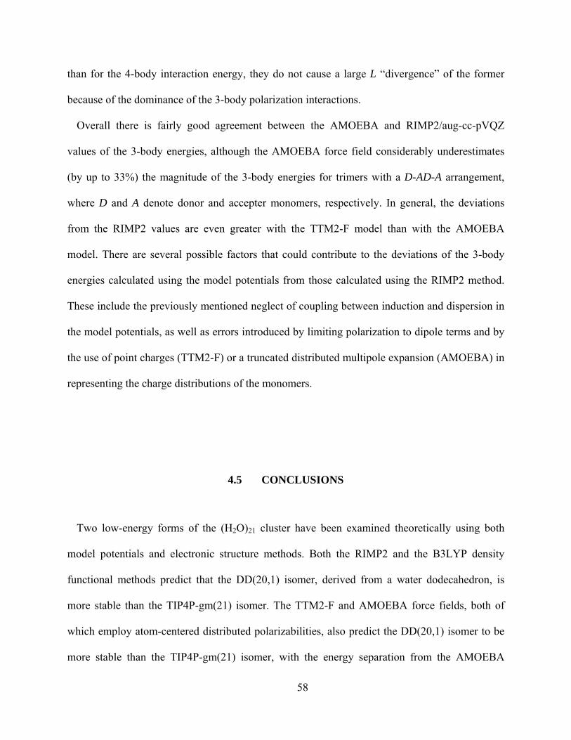
than for the 4-body interaction energy, they do not cause a large L “divergence” of the former
because of the dominance of the 3-body polarization interactions.
Overall there is fairly good agreement between the AMOEBA and RIMP2/aug-cc-pVQZ
values of the 3-body energies, although the AMOEBA force field considerably underestimates
(by up to 33%) the magnitude of the 3-body energies for trimers with a D-AD-A arrangement,
where D and A denote donor and accepter monomers, respectively. In general, the deviations
from the RIMP2 values are even greater with the TTM2-F model than with the AMOEBA
model. There are several possible factors that could contribute to the deviations of the 3-body
energies calculated using the model potentials from those calculated using the RIMP2 method.
These include the previously mentioned neglect of coupling between induction and dispersion in
the model potentials, as well as errors introduced by limiting polarization to dipole terms and by
the use of point charges (TTM2-F) or a truncated distributed multipole expansion (AMOEBA) in
representing the charge distributions of the monomers.
4.5 CONCLUSIONS
Two low-energy forms of the (H2O)21 cluster have been examined theoretically using both
model potentials and electronic structure methods. Both the RIMP2 and the B3LYP density
functional methods predict that the DD(20,1) isomer, derived from a water dodecahedron, is
more stable than the TIP4P-gm(21) isomer. The TTM2-F and AMOEBA force fields, both of
which employ atom-centered distributed polarizabilities, also predict the DD(20,1) isomer to be
more stable than the TIP4P-gm(21) isomer, with the energy separation from the AMOEBA
58
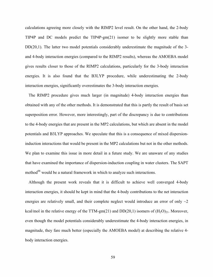
calculations agreeing more closely with the RIMP2 level result. On the other hand, the 2-body
TIP4P and DC models predict the TIP4P-gm(21) isomer to be slightly more stable than
DD(20,1). The latter two model potentials considerably underestimate the magnitude of the 3-
and 4-body interaction energies (compared to the RIMP2 results), whereas the AMOEBA model
gives results closer to those of the RIMP2 calculations, particularly for the 3-body interaction
energies. It is also found that the B3LYP procedure, while underestimating the 2-body
interaction energies, significantly overestimates the 3-body interaction energies.
The RIMP2 procedure gives much larger (in magnitude) 4-body interaction energies than
obtained with any of the other methods. It is demonstrated that this is partly the result of basis set
superposition error. However, more interestingly, part of the discrepancy is due to contributions
to the 4-body energies that are present in the MP2 calculations, but which are absent in the model
potentials and B3LYP approaches. We speculate that this is a consequence of mixed dispersion-
induction interactions that would be present in the MP2 calculations but not in the other methods.
We plan to examine this issue in more detail in a future study. We are unaware of any studies
that have examined the importance of dispersion-induction coupling in water clusters. The SAPT
method98 would be a natural framework in which to analyze such interactions.
Although the present work reveals that it is difficult to achieve well converged 4-body
interaction energies, it should be kept in mind that the 4-body contributions to the net interaction
energies are relatively small, and their complete neglect would introduce an error of only ~2
kcal/mol in the relative energy of the TTM-gm(21) and DD(20,1) isomers of (H2O)21. Moreover,
even though the model potentials considerably underestimate the 4-body interaction energies, in
magnitude, they fare much better (especially the AMOEBA model) at describing the relative 4-
body interaction energies.
59
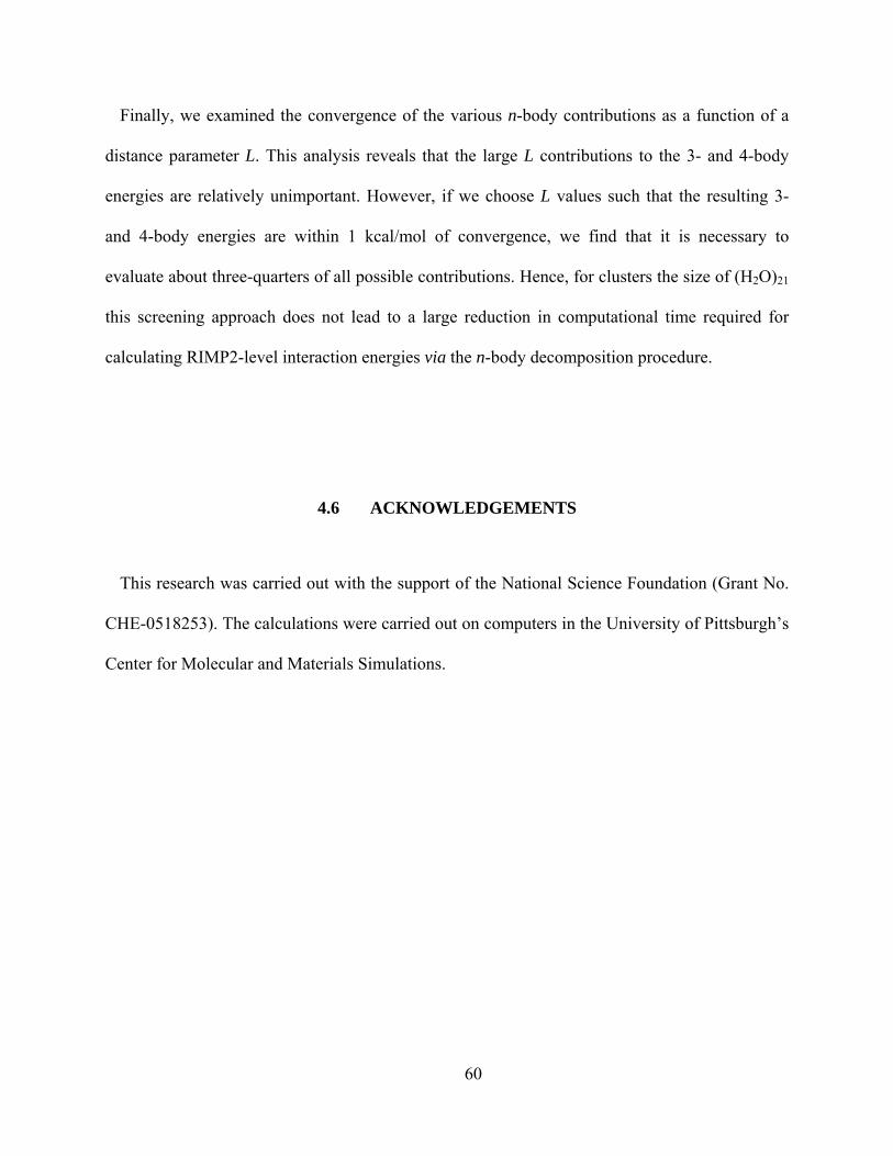
Finally, we examined the convergence of the various n-body contributions as a function of a
distance parameter L. This analysis reveals that the large L contributions to the 3- and 4-body
energies are relatively unimportant. However, if we choose L values such that the resulting 3-
and 4-body energies are within 1 kcal/mol of convergence, we find that it is necessary to
evaluate about three-quarters of all possible contributions. Hence, for clusters the size of (H2O)21
this screening approach does not lead to a large reduction in computational time required for
calculating RIMP2-level interaction energies via the n-body decomposition procedure.
4.6 ACKNOWLEDGEMENTS
This research was carried out with the support of the National Science Foundation (Grant No.
CHE-0518253). The calculations were carried out on computers in the University of Pittsburgh’s
Center for Molecular and Materials Simulations.
60
Figure 17. RIMP2/aug-cc-pVDZ optimized geometries of the (a) DD(20,1) and (b) TIP4P-
gm(21) isomers of (H2O)21 and of the (c) D(19,1), (d) pentagonal prism [PP(20)], and (e)
“perfect” dodecahedron [PD(20)] isomers of (H2O)20.
61
Figure 18. Interaction energies for the DD(20,1) and TIP4P-gm(21) isomers of (H2O)21 and of
various forms of (H2O)20 calculated using the TIP4P, DC, TTM2-F, AMOEBA, B3LYP/aug-cc-
pVTZ(-f), and RIMP2/aug-cc-pVTZ(-f) methods.
62
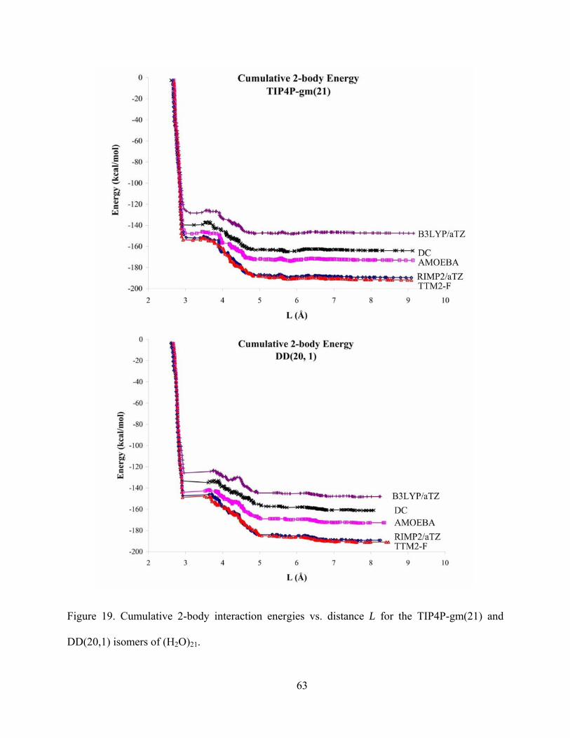
Figure 19. Cumulative 2-body interaction energies vs. distance L for the TIP4P-gm(21) and
DD(20,1) isomers of (H2O)21.
63
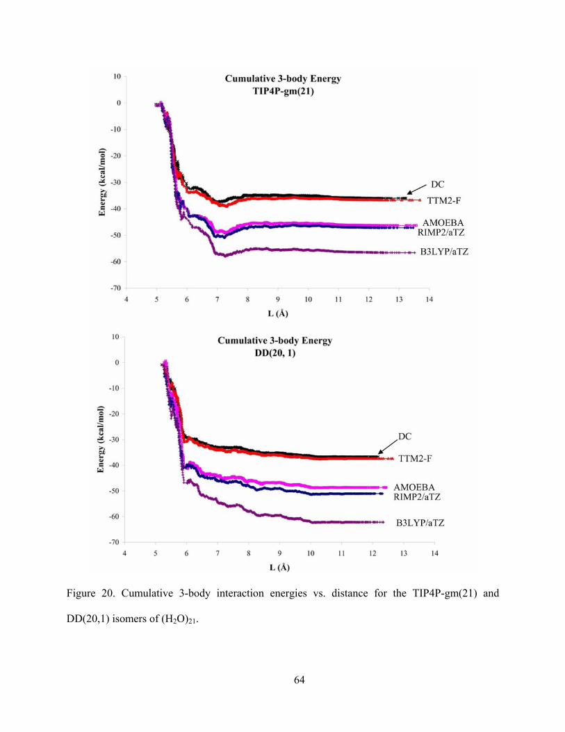
Figure 20. Cumulative 3-body interaction energies vs. distance for the TIP4P-gm(21) and
DD(20,1) isomers of (H2O)21.
64
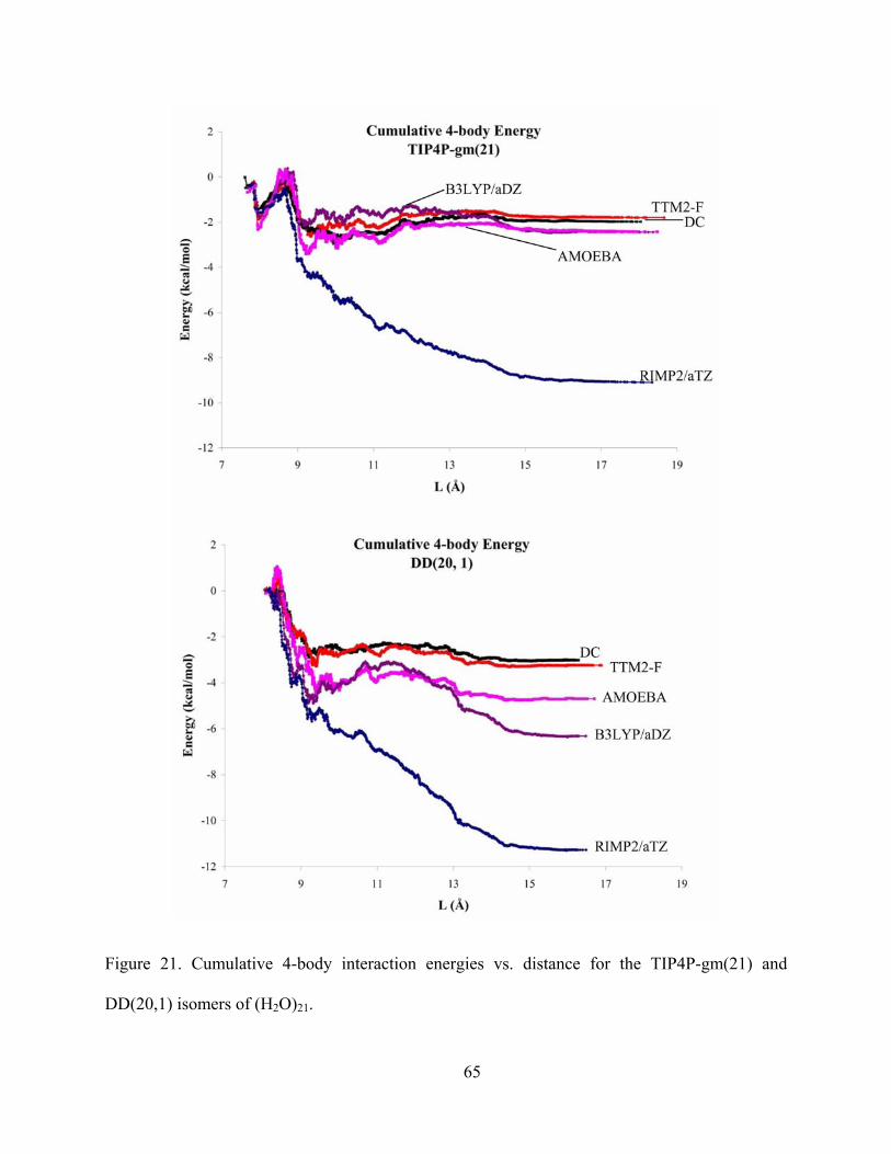
Figure 21. Cumulative 4-body interaction energies vs. distance for the TIP4P-gm(21) and
DD(20,1) isomers of (H2O)21.
65
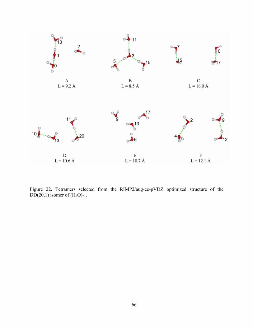
Figure 22. Tetramers selected from the RIMP2/aug-cc-pVDZ optimized structure of the DD(20,1) isomer of (H2O)21.
66
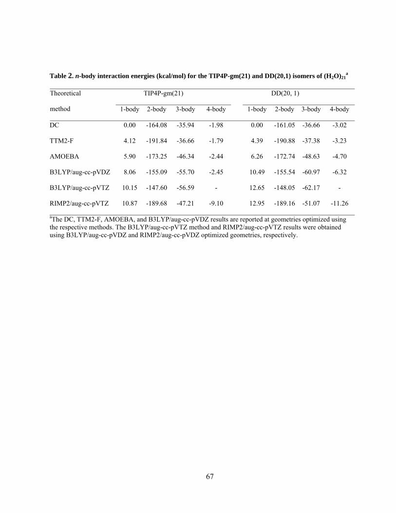
Table 2. n-body interaction energies (kcal/mol) for the TIP4P-gm(21) and DD(20,1) isomers of (H2O)21a
TIP4P-gm(21) DD(20, 1) Theoretical
method 1-body 2-body 3-body 4-body 1-body 2-body 3-body 4-body
DC 0.00 -164.08 -35.94 -1.98 0.00 -161.05 -36.66 -3.02
TTM2-F 4.12 -191.84 -36.66 -1.79 4.39 -190.88 -37.38 -3.23
AMOEBA 5.90 -173.25 -46.34 -2.44 6.26 -172.74 -48.63 -4.70
B3LYP/aug-cc-pVDZ 8.06 -155.09 -55.70 -2.45 10.49 -155.54 -60.97 -6.32
B3LYP/aug-cc-pVTZ 10.15 -147.60 -56.59 - 12.65 -148.05 -62.17 -
RIMP2/aug-cc-pVTZ 10.87 -189.68 -47.21 -9.10 12.95 -189.16 -51.07 -11.26
aThe DC, TTM2-F, AMOEBA, and B3LYP/aug-cc-pVDZ results are reported at geometries optimized using the respective methods. The B3LYP/aug-cc-pVTZ method and RIMP2/aug-cc-pVTZ results were obtained using B3LYP/aug-cc-pVDZ and RIMP2/aug-cc-pVDZ optimized geometries, respectively.
67
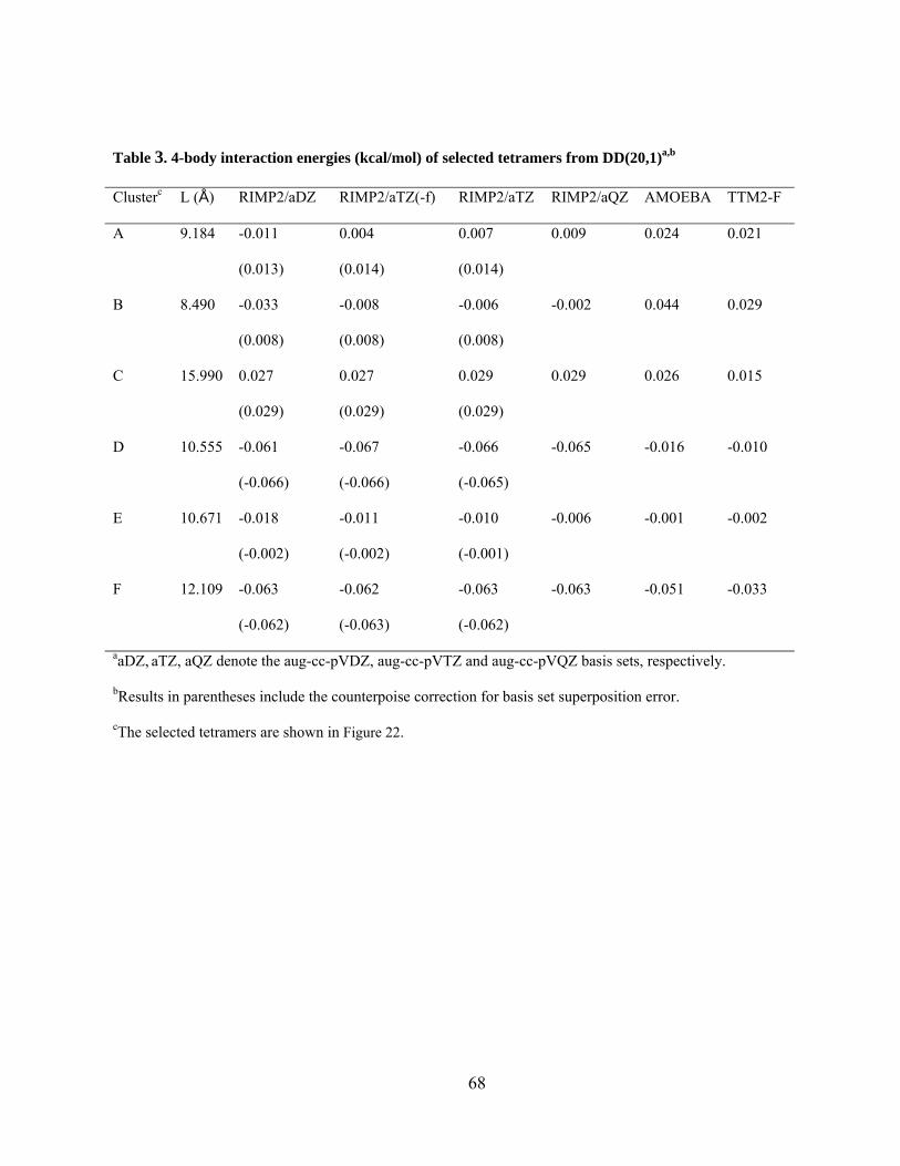
Table 3. 4-body interaction energies (kcal/mol) of selected tetramers from DD(20,1)a,b
Clusterc L (Å) RIMP2/aDZ RIMP2/aTZ(-f) RIMP2/aTZ RIMP2/aQZ AMOEBA TTM2-F
A 9.184 -0.011 0.004 0.007 0.009 0.024 0.021
(0.013) (0.014) (0.014)
B 8.490 -0.033 -0.008 -0.006 -0.002 0.044 0.029
(0.008) (0.008) (0.008)
C 15.990 0.027 0.027 0.029 0.029 0.026 0.015
(0.029) (0.029) (0.029)
D 10.555 -0.061 -0.067 -0.066 -0.065 -0.016 -0.010
(-0.066) (-0.066) (-0.065)
E 10.671 -0.018 -0.011 -0.010 -0.006 -0.001 -0.002
(-0.002) (-0.002) (-0.001)
F 12.109 -0.063 -0.062 -0.063 -0.063 -0.051 -0.033
(-0.062) (-0.063) (-0.062)
aaDZ, aTZ, aQZ denote the aug-cc-pVDZ, aug-cc-pVTZ and aug-cc-pVQZ basis sets, respectively.
bResults in parentheses include the counterpoise correction for basis set superposition error.
cThe selected tetramers are shown in Figure 22.
68
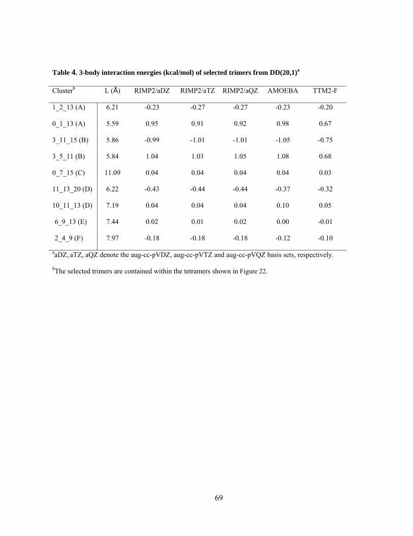
Table 4. 3-body interaction energies (kcal/mol) of selected trimers from DD(20,1)a
Clusterb L (Å) RIMP2/aDZ RIMP2/aTZ RIMP2/aQZ AMOEBA TTM2-F
1_2_13 (A) 6.21 -0.23 -0.27 -0.27 -0.23 -0.20
0_1_13 (A) 5.59 0.95 0.91 0.92 0.98 0.67
3_11_15 (B) 5.86 -0.99 -1.01 -1.01 -1.05 -0.75
3_5_11 (B) 5.84 1.04 1.03 1.05 1.08 0.68
0_7_15 (C) 11.09 0.04 0.04 0.04 0.04 0.03
11_13_20 (D) 6.22 -0.43 -0.44 -0.44 -0.37 -0.32
10_11_13 (D) 7.19 0.04 0.04 0.04 0.10 0.05
6_9_13 (E) 7.44 0.02 0.01 0.02 0.00 -0.01
2_4_9 (F) 7.97 -0.18 -0.18 -0.18 -0.12 -0.10
aaDZ, aTZ, aQZ denote the aug-cc-pVDZ, aug-cc-pVTZ and aug-cc-pVQZ basis sets, respectively.
bThe selected trimers are contained within the tetramers shown in Figure 22.
69
5.0 MANY BODY DECOMPOSITION STUDY OF THE (H2O)21 CLUSTER
5.1 ABSTRACT
The distributions of the relative 2-body, 3-body, and 4-body energies from the RIMP2,
Hartree Fock, B3LYP, and AMOEBA methods vs. the sum of the monomer distances to the
center of mass of the subclusters are reported. It is found that the subclusters with similar
hydrogen bonding arrangements tend to cluster on the distribution plots. The differences between
the predictions from the RIMP2, Hartree Fock, B3LYP and AMOEBA methods is closely related
to the hydrogen bonding patterns of the subclusters.
Typical tetramer structures “3-5-11-15” and “9-12-14-19” have been chosen to analyze
the 4-body energy change as the tetramer “size” increases. For “3-5-11-15”, it is found that the
MP2 and Hartree Fock methods give attractive 4-body energy values, and the B3LYP and
AMOEBA methods give repulsive values. Further energy component analysis with the KM and
RVS methods reveal that the differences might be a result of the exchange effects. It was also
found the tetramers with the “A/AAD/D/D” hydrogen bonding pattern contribute to the
differences between the cumulative 4-body energies calculated using the MP2 and the HF,
B3LYP, and AMOEBA methods.
70
5.2 INTRODUCTION
The most straightforward method to describe the weak interaction between water
molecules is to evaluate the electronic energy of the whole system. The interaction energy is
computed by substracting the energy of the whole system and the sum of the interacting parties.
This standard method is called the “supermolecule” method, or the whole system method.
However, for large cluster size, only simple methods such as the Hartree Fock (HF), density
functional theory (DFT) with small basis set and model potentials are possible for the whole
system method due to high computational cost. Also, the whole system method only gives the
total energy of the whole system and is very limited in explaining the physical meaning of the
data.
The intermolecular interaction between water molecules is complicated due to the
presence of non-additive components, such as the polarization and exchange effects. The
question remains if the approximations adopted by the simpler methods can reproduce the non-
additive terms. For example, in the model potentials, some of the interactions are distorted to
mimic the non-additive terms.77,79,85,86,99-101 While these models can reproduce the properties of
liquid water phase, they often fail to reproduce the properties of small water clusters and also
make the simulation data hard to interpret.66
An alternative to the “supermolecule” method is the energy component analysis method.
The energy component analysis classifies the intermolecular interaction energy into different
physical components, and then use ab initio approaches to understand the fundamental physical
components behind the intermolecular interaction. It provides additional insight into the
importance of various terms in the intermolecular potential, and helps to develop more advanced
model potentials.
71
There are several ways to partition the interaction energy at the Hartree Fock level of
theory, such as the Kitaura-Morokuma (KM) analysis,102-104 the reduced variational space self-
consistent-field (RVS SCF) method (also known as the constrained space orbital variation
(CSOV) method),105,106 and the symmetry adapted perturbation theory (SAPT).107-114
In this work, we will give a detailed comparison of the n-body energies (n≤4) from the
MP2, B3LYP, HF, and AMOEBA methods. The KM and RVS energy component analysis
methods are then used to explore the difference between the four theoretical methods.
5.3 COMPUTATIONAL DETAILS
The geometry of the DD(20, 1) isomer of the (H2O)21 cluster was optimized with the
RIMP2 procedures using the aug-cc-pVDZ basis sets.89,90 The optimized geometry was then
decomposed into dimers, trimers, and tetramers with a home developed interface.
The n-body decomposition was performed by calculating the energies of the various
monomers, dimers, trimers, and tetramer subclusters present in the (H2O)21 clusters. The energies
from the subcluster calculations were used to evaluate the 2-, 3-, and 4-body interaction energies
as a function of a variable L, taken to be the sum of the distances from the center of mass of the
subcluster to the individual centers of mass of the monomers in the subcluster. L thus provides a
measure of the “size” of the subcluster. In the electronic structure calculations of the individual
n-body interaction energy, the full aug-cc-pVTZ basis set was employed for the RIMP2 and
B3LYP calculations, with the exception of the B3LYP 4-body results, which were obtained with
the aug-cc-pVDZ basis set.
72
The B3LYP and RIMP2 calculations were carried out using Gaussian 0359 and
Turbomole,91,92 respectively. The calculations with the AMOEBA force fields was carried out
using the Tinker program.86,93-95 The AMOEBA model employs flexible monomers and three
atom-centered, mutually interacting, polarizable sites. The model uses distributed multipoles
through quadrupoles on the three atoms on a water monomer to represent the charge distribution.
It employs buffered 7–14 OO, HH, and HO potentials to represent the dispersion interactions and
short-range repulsion. AMOEBA uses a Thole-type damping96 of the charge–induced dipole
interactions and also of the induced dipole–induced dipole interactions. The energy
decomposition analysis was carried out with the KM and RVS methods using the GAMESS
software package.115,116
5.4 RESULTS AND DISCUSSION
In section 4.0, it was found that the MP2 method gave a much lower cumulative 4-body
energy than obtained with the B3LYP, AMOEBA, TTM, and Dang-Chang methods. The reason
for this was not obvious. This chapter will present a detailed theoretical study of the DD(20,1)
isomer of the (H2O)21 cluster, with an emphasis on elucidating the level of theory needed to
accurately describe the n-body (n = 2, 3, and 4) interaction energies. In this analysis, results from
the B3LYP density functional80-82 and the HF electronic structure methods, as well as from the
AMOEBA86 polarizable water model are compared to those from the RIMP283,84 calculations.
73
5.4.1 n-body energy distribution for DD(20,1) subclusters
The DD(20, 1) isomer of the (H2O)21 cluster can be decomposed into 210 dimers, 1350
trimers, and 5985 tetramers. The subclusters are categorized according to their hydrogen
donating and accepting properties. For each subcluster, hydrogen bonds are deemed to exist
whenever the distance between the oxygen atom in one water molecule and a hydrogen atom in
another water molecule is in the range of 1.2 – 2.2 Å. A water molecule can donate its two
hydrogen atoms (so called “D” type), or accept two hydrogen atoms (so called “A” type) to form
hydrogen bonds with other water molecules.
For the 210 dimers obtained, there are two possible types: “A/D” or “-/-“. A dimer is
counted as “A/D” if there is an H-bond and “-/-” if there is none, with the above definition.
Figure 23 exhibits the MP2-HF (Figure 23(a)), MP2-B3LYP (Figure 23(b)), and MP2-
AMOEBA (Figure 23(c)) differences for the 2-body energies as a function of L. Each point in
the figure corresponds to a dimer structure.
There are two distinctive groups in all three figures (as shown in Figure 23 (a)-(c)). For
the “A/D” type dimers at short distances, when compared to the MP2 method, the 2-body energy
is about 1.5-2.8 kcal/mol less attractive with the HF method (Figure 23(a)), and 0.39-0.49
kcal/mol less attractive with the B3LYP (Figure 23(b)) method. The AMOEBA results range
from 0.22 kcal/mol less attractive to 0.45 kcal/mol more attractive than the MP2 results.
There are systematic differences between the 2-body energies from the MP2 method and
those from the HF and B3LYP methods. A major factor contributing to the larger (in magnitude)
2-body interaction energies in the MP2 method than in the HF or B3LYP methods is dispersion.
Further analysis will elucidate the exact contributions to the energy difference.
74
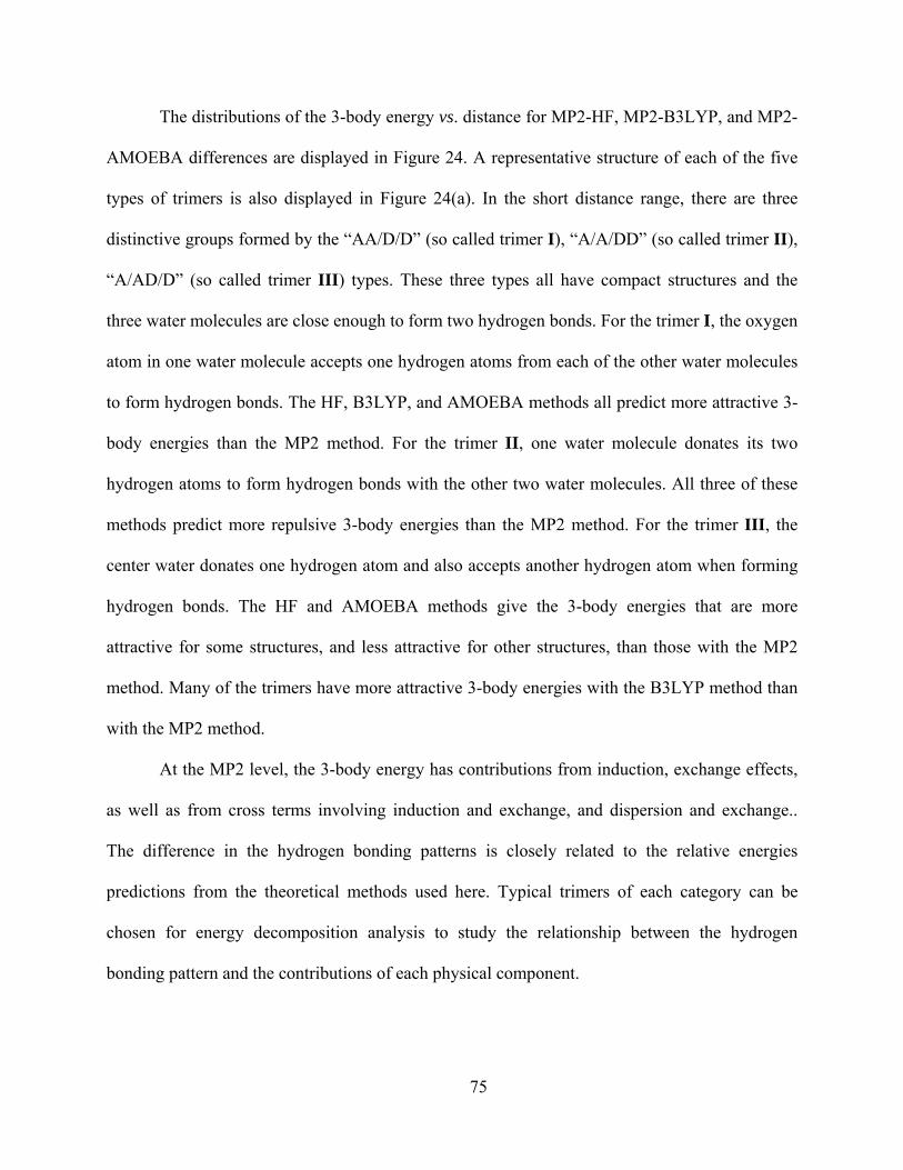
The distributions of the 3-body energy vs. distance for MP2-HF, MP2-B3LYP, and MP2-
AMOEBA differences are displayed in Figure 24. A representative structure of each of the five
types of trimers is also displayed in Figure 24(a). In the short distance range, there are three
distinctive groups formed by the “AA/D/D” (so called trimer I), “A/A/DD” (so called trimer II),
“A/AD/D” (so called trimer III) types. These three types all have compact structures and the
three water molecules are close enough to form two hydrogen bonds. For the trimer I, the oxygen
atom in one water molecule accepts one hydrogen atoms from each of the other water molecules
to form hydrogen bonds. The HF, B3LYP, and AMOEBA methods all predict more attractive 3-
body energies than the MP2 method. For the trimer II, one water molecule donates its two
hydrogen atoms to form hydrogen bonds with the other two water molecules. All three of these
methods predict more repulsive 3-body energies than the MP2 method. For the trimer III, the
center water donates one hydrogen atom and also accepts another hydrogen atom when forming
hydrogen bonds. The HF and AMOEBA methods give the 3-body energies that are more
attractive for some structures, and less attractive for other structures, than those with the MP2
method. Many of the trimers have more attractive 3-body energies with the B3LYP method than
with the MP2 method.
At the MP2 level, the 3-body energy has contributions from induction, exchange effects,
as well as from cross terms involving induction and exchange, and dispersion and exchange..
The difference in the hydrogen bonding patterns is closely related to the relative energies
predictions from the theoretical methods used here. Typical trimers of each category can be
chosen for energy decomposition analysis to study the relationship between the hydrogen
bonding pattern and the contributions of each physical component.
75
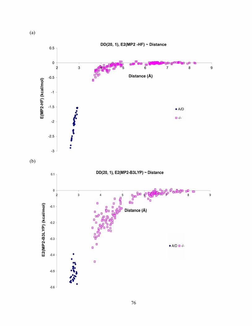
(a)
(b)
76
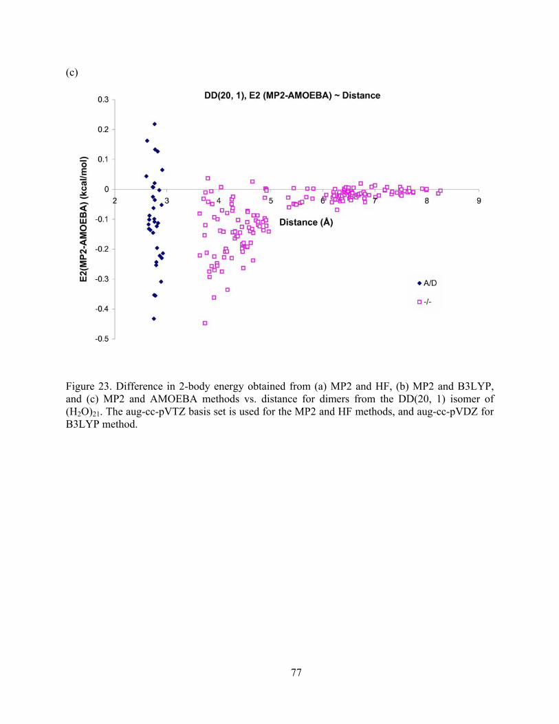
(c)
Figure 23. Difference in 2-body energy obtained from (a) MP2 and HF, (b) MP2 and B3LYP, and (c) MP2 and AMOEBA methods vs. distance for dimers from the DD(20, 1) isomer of (H2O)21. The aug-cc-pVTZ basis set is used for the MP2 and HF methods, and aug-cc-pVDZ for B3LYP method.
77
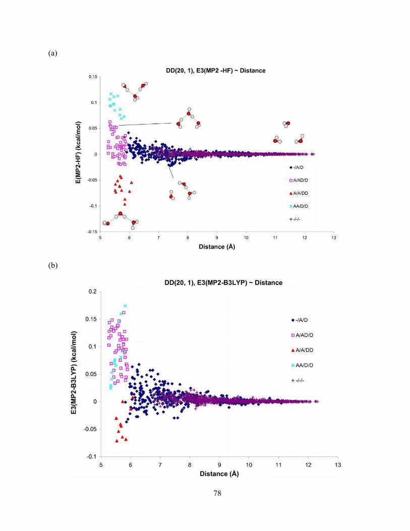
(a)
(b)
78
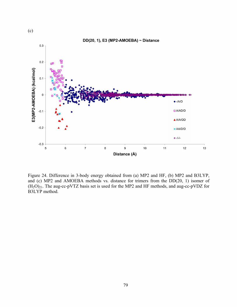
(c)
Figure 24. Difference in 3-body energy obtained from (a) MP2 and HF, (b) MP2 and B3LYP, and (c) MP2 and AMOEBA methods vs. distance for trimers from the DD(20, 1) isomer of (H2O)21. The aug-cc-pVTZ basis set is used for the MP2 and HF methods, and aug-cc-pVDZ for B3LYP method.
79
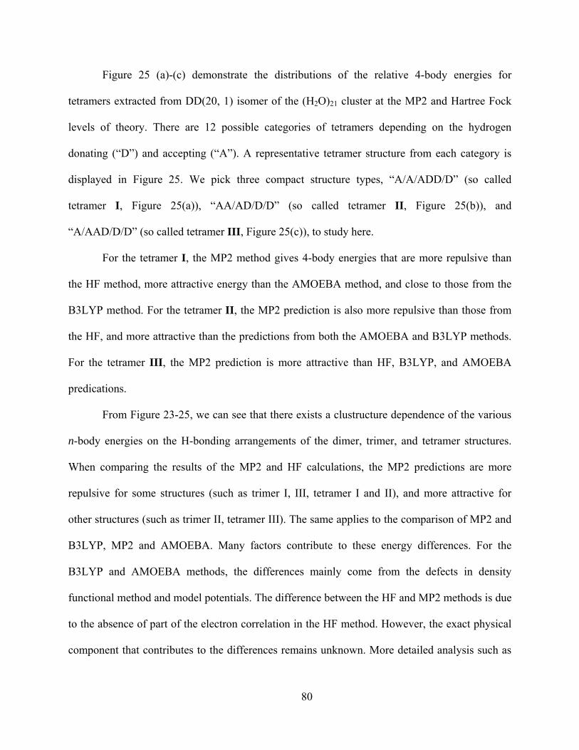
Figure 25 (a)-(c) demonstrate the distributions of the relative 4-body energies for
tetramers extracted from DD(20, 1) isomer of the (H2O)21 cluster at the MP2 and Hartree Fock
levels of theory. There are 12 possible categories of tetramers depending on the hydrogen
donating (“D”) and accepting (“A”). A representative tetramer structure from each category is
displayed in Figure 25. We pick three compact structure types, “A/A/ADD/D” (so called
tetramer I, Figure 25(a)), “AA/AD/D/D” (so called tetramer II, Figure 25(b)), and
“A/AAD/D/D” (so called tetramer III, Figure 25(c)), to study here.
For the tetramer I, the MP2 method gives 4-body energies that are more repulsive than
the HF method, more attractive energy than the AMOEBA method, and close to those from the
B3LYP method. For the tetramer II, the MP2 prediction is also more repulsive than those from
the HF, and more attractive than the predictions from both the AMOEBA and B3LYP methods.
For the tetramer III, the MP2 prediction is more attractive than HF, B3LYP, and AMOEBA
predications.
From Figure 23-25, we can see that there exists a clustructure dependence of the various
n-body energies on the H-bonding arrangements of the dimer, trimer, and tetramer structures.
When comparing the results of the MP2 and HF calculations, the MP2 predictions are more
repulsive for some structures (such as trimer I, III, tetramer I and II), and more attractive for
other structures (such as trimer II, tetramer III). The same applies to the comparison of MP2 and
B3LYP, MP2 and AMOEBA. Many factors contribute to these energy differences. For the
B3LYP and AMOEBA methods, the differences mainly come from the defects in density
functional method and model potentials. The difference between the HF and MP2 methods is due
to the absence of part of the electron correlation in the HF method. However, the exact physical
component that contributes to the differences remains unknown. More detailed analysis such as
80

interaction energy decomposition is needed. Next, we will study a typical subcluster, aiming at
the difference between the MP2 and other methods.
81
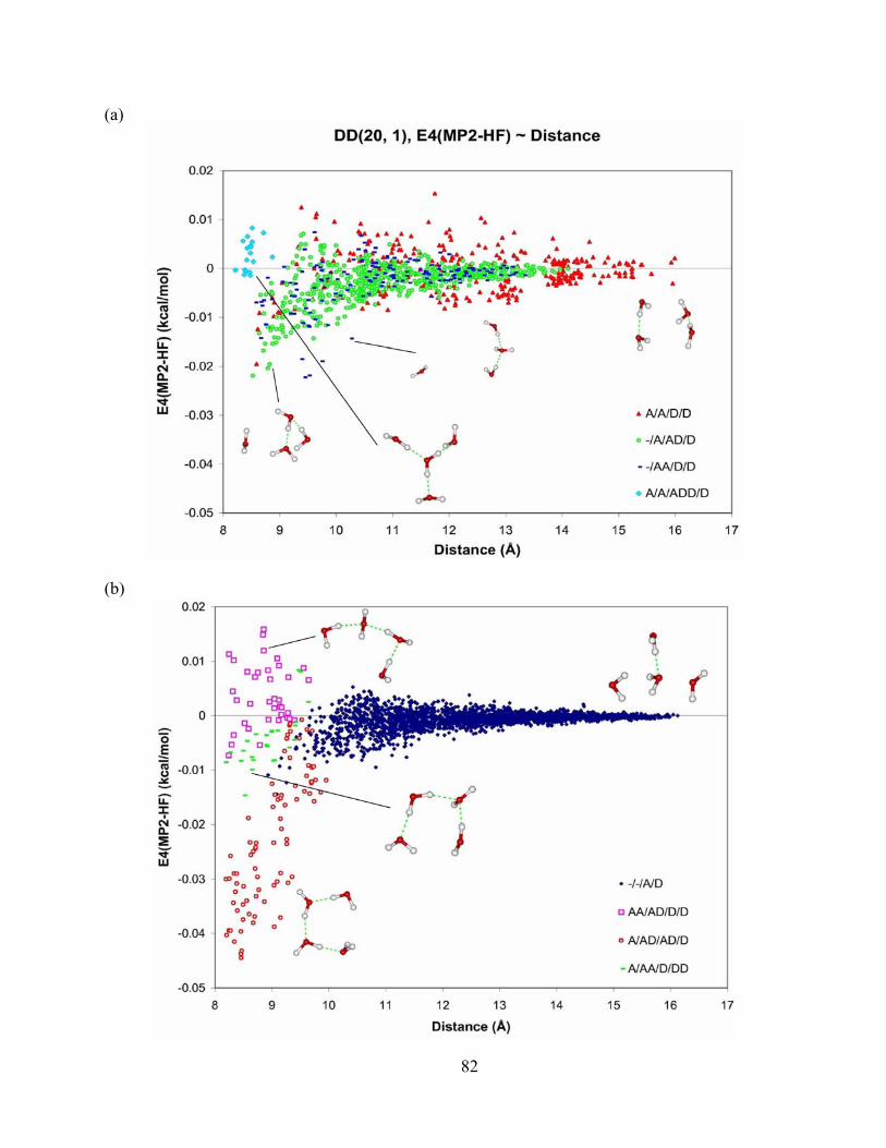
(a)
(b)
82
Figure 25. Difference in 4-body energy obtained from MP2 and HF methods vs. distance for tetramers from DD(20, 1) isomer of (H2O)21. The aug-cc-pVTZ basis set is used for the MP2 and HF methods. The DD(20, 1) isomer of (H2O)21 was optimized at the MP2 level of theory and aug-cc-pVDZ basis set.
(c )
83
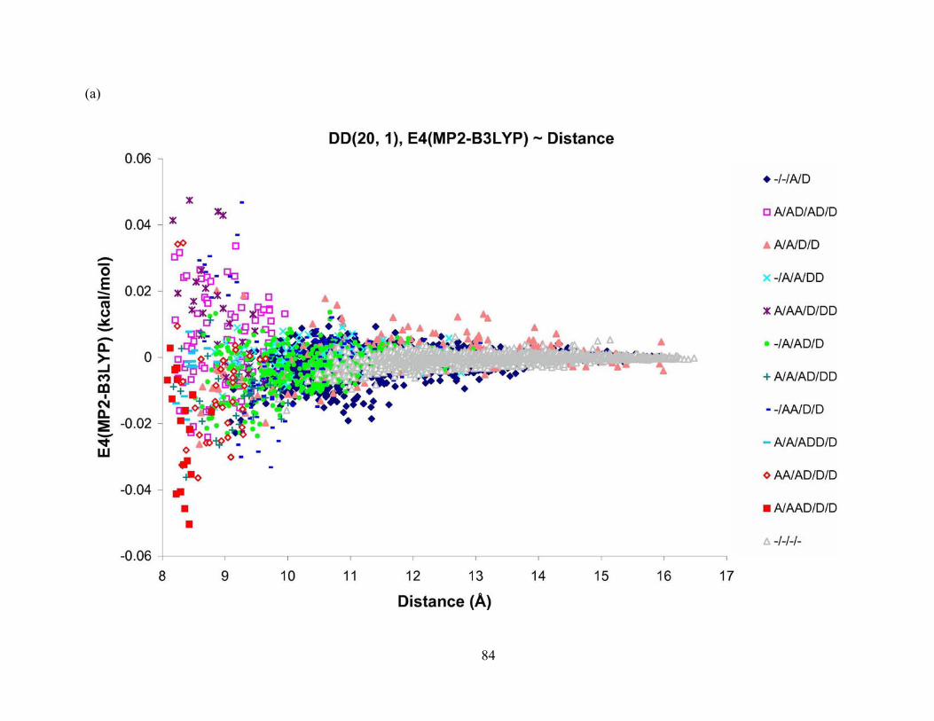
(a)
84
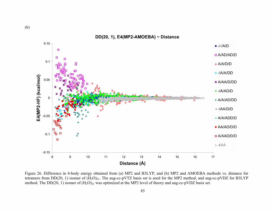
Figure 26. Difference in 4-body energy obtained from (a) MP2 and B3LYP, and (b) MP2 and AMOEBA methods vs. distance for tetramers from DD(20, 1) isomer of (H2O)21. The aug-cc-pVTZ basis set is used for the MP2 method, and aug-cc-pVDZ for B3LYP method. The DD(20, 1) isomer of (H2O)21 was optimized at the MP2 level of theory and aug-cc-pVDZ basis set.
85
(b)
5.4.2 Structural analysis for typical tetramers
As shown in Figures 25 and 26, there are differences between the 4-body energies
predicted by the MP2 and HF, B3LYP, AMOEBA methods. The energy difference is closely
related to the structure and hydrogen bonding pattern of the tetramer studied. In this part of the
work, we will focus on selected structures from the tetramer I (“A/A/ADD/D”, as shown in
Figure 25(a)) and the tetramer III (“A/AAD/D/D”, as shown in Figure 25(c)) types. A tetramer
structure from each type is chosen: “3-5-11-15” from type I (structure shown in Figure 27(a)),
and “9-12-14-19” from type III (structure shown in Figure 28(a)).
Tetramer “3-5-11-15” has a planar structure with 3 hydrogen bonds between the center
water molecule 3 and other water molecules around it. Water molecule 15 is pulled away
gradually relative to water 3 at the center. The distance between 3 and 15 is measured as the
separation between the two oxygen atoms. Water 15 is moved away by 0.5 Å at each step. The 4-
body energy of each resulting structure is calculated at the MP2, HF, B3LYP level of theory, and
with the AMOEBA force field. We use the aug-cc-pVTZ basis set for the electronic structure
calculations. An ultrafine grid is used for the B3LYP integration.
Figure 27(b) exhibits the dependence of the 4-body energy on the O(3)-O(15) distance.
The 4-body energy predicted by the MP2 method decreases first as the distance increases from
2.7 Å to 3.2 Å, and then increases in similar trend to the HF method. Both the B3LYP and
AMOEBA methods give repulsive 4-body energies at all distances. AMOEBA’s prediction is
clearly markedly different from that from the other methods. As distance increases, the energies
from different methods slowly converge to ~ 0.002 kcal/mol.
86
Similar calculations are done on the “9-12-14-19” tetramer. The center water 9 has the
“AAD” hydrogen bonding pattern, while the center water 3 of “3-5-11-15” has the “ADD”
hydrogen bonding pattern. Water 19 is pulled away relative to 9 (as shown in Figure 28(a)).
Figure 28(b) demonstrates the dependence of the 4-body energy on the O(9)-O(19) distance. All
the methods predict repulsive 4-body energies except the MP2 method in the 4.5-5.5 Å range.
The 4-body energies predicted by the MP2 method are much lower than those by the HF and
B3LYP methods. The AMOEBA predictions are very different from the other methods. It is
reasonable to assume that the type III tetramers may have similar 4-body energy dependence on
the distance to that of “9-12-14-19”. This is confirmed by their distributions on Figure 25(c) and
26. The type III tetramers certainly contribute to the difference in the cumulative 4-body
energies between the MP2 and the other methods as discussed in section 4.0 (Figure 21).
In Figure 27, it is interesting that the MP2 method gives the opposite sign for the 4-body
interaction than found with the B3LYP, AMOEBA methods. Figure 29 shows how the 4-body
induction energy changes as water 15 is pulled away in the “3-5-11-15” tetramer (I thank Albert
Defusco for his contribution to the figure). The RVS and KM models produce totally different
results for the 4-body induction energy. The KM method gives repulsive induction energies
while the RVS gives attractive induction energies. The pattern of the energy changes in Figure
29 is similar to what we saw in Figure 27(b) (at least for L ≥ 4.5 Å).
The KM analysis splits the Hartree Fock interaction energy into electrostatic, exchange,
polarization, and charge transfer components. A major drawback of the KM method is that the
impact of exchange on the induction is not included. The RVS method is similar to the KM
analysis except that the wave functions involved in the decomposition process satisfy the Pauli
exclusion principle. These results show that the inclusion of exchange interations reverse the sign
87
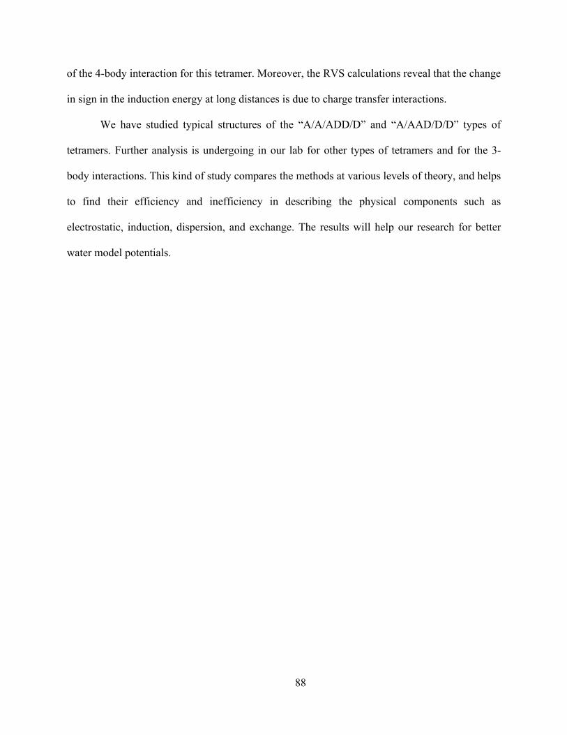
of the 4-body interaction for this tetramer. Moreover, the RVS calculations reveal that the change
in sign in the induction energy at long distances is due to charge transfer interactions.
We have studied typical structures of the “A/A/ADD/D” and “A/AAD/D/D” types of
tetramers. Further analysis is undergoing in our lab for other types of tetramers and for the 3-
body interactions. This kind of study compares the methods at various levels of theory, and helps
to find their efficiency and inefficiency in describing the physical components such as
electrostatic, induction, dispersion, and exchange. The results will help our research for better
water model potentials.
88
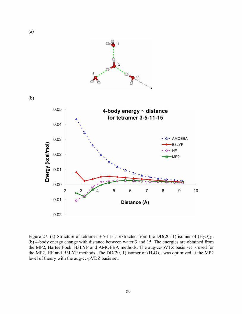
(a)
(b)
Figure 27. (a) Structure of tetramer 3-5-11-15 extracted from the DD(20, 1) isomer of (H2O)21. (b) 4-body energy change with distance between water 3 and 15. The energies are obtained from the MP2, Hartee Fock, B3LYP and AMOEBA methods. The aug-cc-pVTZ basis set is used for the MP2, HF and B3LYP methods. The DD(20, 1) isomer of (H2O)21 was optimized at the MP2 level of theory with the aug-cc-pVDZ basis set.
89
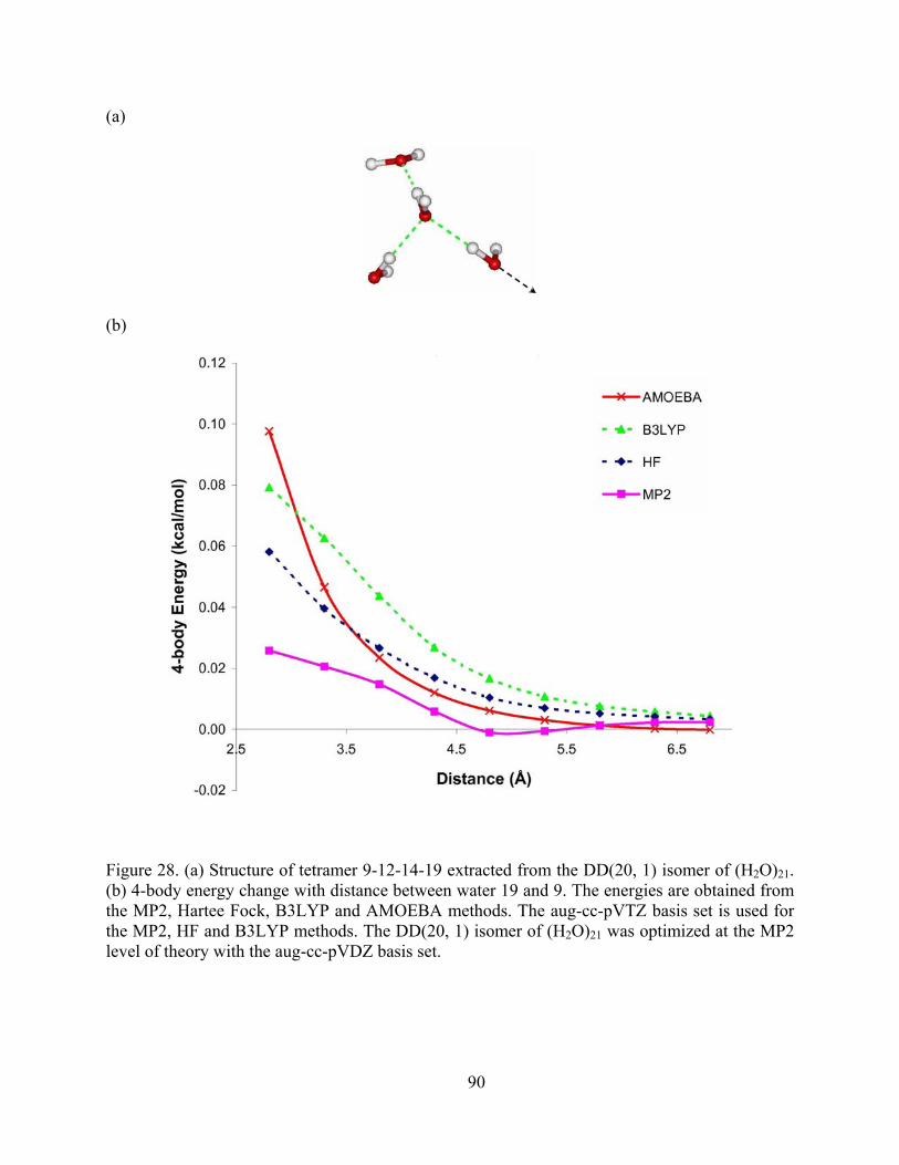
(a)
(b)
Figure 28. (a) Structure of tetramer 9-12-14-19 extracted from the DD(20, 1) isomer of (H2O)21. (b) 4-body energy change with distance between water 19 and 9. The energies are obtained from the MP2, Hartee Fock, B3LYP and AMOEBA methods. The aug-cc-pVTZ basis set is used for the MP2, HF and B3LYP methods. The DD(20, 1) isomer of (H2O)21 was optimized at the MP2 level of theory with the aug-cc-pVDZ basis set.
90
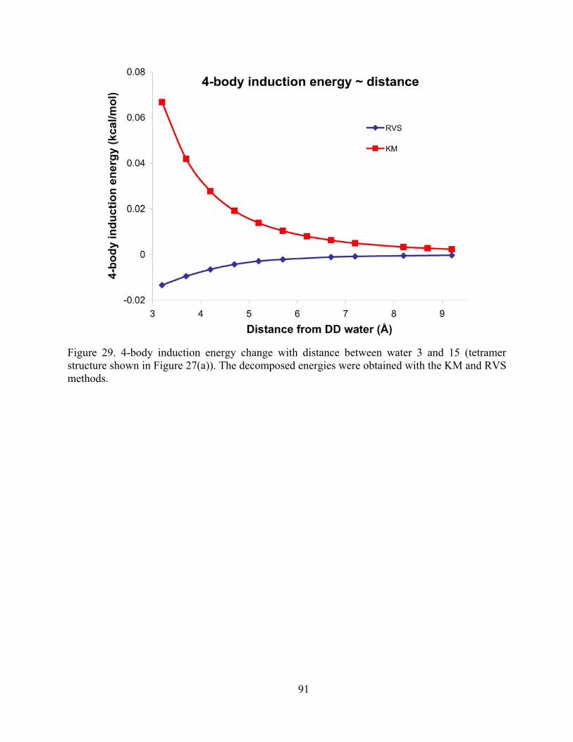
Figure 29. 4-body induction energy change with distance between water 3 and 15 (tetramer structure shown in Figure 27(a)). The decomposed energies were obtained with the KM and RVS methods.
91
5.5 CONCLUSIONS
We have studied the distributions of 2-body, 3-body, and 4-body energies. The energy
dependences on the distance were studied and simulation results with the RIMP2, Hartree Fock,
B3LYP, and AMOEBA methods were compared. The tetramers extracted from the DD(20, 1)
isomer of the (H2O)21 cluster were categorized into 12 types according to their hydrogen
donating and accepting numbers. The distribution of 4-body energy showed a strong dependence
on the tetramer types.
Typical tetramer structures “3-5-11-15” and “9-12-14-19” have been chosen to analyze
the 4-body energy change as one of the water molecules was pulled away. For tetramer “3-5-11-
15”, it was found that the MP2 and HF methods gave attractive 4-body energy values, and the
B3LYP and AMOEBA methods gave repulsive values. Further energy component analysis with
the KM and RVS methods revealed that the 4-body induction energy had a positive value with
the KM method, and a negative value with the RVS method. This indicates that the differences
between the 4-body energies calculated using the MP2 and B3LYP, AMOEBA methods might
be a result of the exchange effects. For tetramer “9-12-14-19”, the MP2 method predicts much
lower 4-body energy than the other methods. The tetramers with the “A/AAD/D/D” hydrogen
bonding pattern contribute to the differences between the cumulative 4-body energies calculated
using the MP2 and the HF, B3LYP, and AMOEBA methods. This is further confirmed by the 4-
body distributions in Figure 25 and 26.
Further research with the KM, RVS and SAPT methods in the energy partition of the
water trimers and tetramers are undergoing in our lab.
92

5.6 ACKNOWLEDGEMENTS
This research was carried out with the support of the National Science Foundation (Grant
No. CHE-0518253). The calculations were carried out on computers in the University of
Pittsburgh’s Center for Molecular and Materials Simulations.
93
APPENDIX: MONITORING THE ACTIVITY OF BRAIN CHOLINERGIC SYSTEMS
This work was published as:
Cui J., Kulagina N.V., Michael A.C., J. Neuroscience Methods 104 183-189 (2001).117
ABSTRACT
Monitoring the levels of neurotransmitters in the extracellular space of living brain is
challenging because the lifetime of these important compounds is very short. For example,
acetylcholine is rapidly metabolized in the extracellular space by cholinesterase enzymes. For
this reason, acetylcholine may be metabolized before it reaches an implanted sampling probe,
such as a microdialysis probe.
In this project, we have constructed enzyme-modified carbon fiber microelectrodes that
are suitable for the detection of choline in the extracellular space of the living brain. The
advantage of these devices is that they are implanted into the brain. As a consequence, the
microelectrode can be placed very close to viable neuronal terminals. We have investigated
whether or not the signal observed in the brain with these microelectrodes is related to the
activity of cholinergic neurons.
Amperometric microsensors have been developed for the in vivo detection of choline and
glucose. Choline oxidase, horseradish peroxidase and glucose oxidase were immobilized in a
crosslinked redox polymer matrix on carbon fiber electrodes. Choline microsensors gave a
detection limit of 1~3 μM. Optimized glucose microsensors gave a detection limit of ~100 μM-
94
200 μM and a linear response up to 10 mM, which includes the physiologically relevant glucose
concentration. Immobilization of ascorbate oxidase and a Nafion outlayer gave selectivity above
90% to both choline microsensors and glucose microsensors over 400 μM ascorbate, which is the
physiologically relevant concentration.
We have tested whether or not the cholinergic signal is useful as an index of cholinergic
brain activity. We have observed that when tetrodotoxin (TTX) is infused into brain tissue near
the microsensors, the signal decreases. Since TTX causes neuronal activity to stop, this result
suggests that the choline signal may indeed provide a useful index of acetylcholine release.
Furthermore, the signals also decrease when neostigmine, a powerful cholinesterase inhibitor, is
infused into the brain tissue. Neither TTX nor neostigmine infusions into brain tissue influence
the signal recorded with glucose oxidase modified microelectrodes. These results suggest that
enzyme-modified microelectrodes are indeed a potential index of acetylcholine release.
INTRODUCTION
Acetylcholine is a very important neurotransmitter in the brain. It is related to many
diseases, such as Alzheimer’s disease, Huntington’s disease, Parkinson’s disease etc.118,119
Despite the fact that it was the first neurotransmitter discovered,120 acetylcholine remains
difficult to study in the brain due to many reasons. Acetylcholine hydrolyzes easily in
extracellular space to choline and acetic acid under the catalysis of cholinesterase. This can
happen before acetylcholine reaches the detector and makes the basal concentration of
acetylcholine in the extracellular space very low (~nM).121 The basal extracellular acetylcholine
concentration is usually below the detection limit of most detectors. Also, acetylcholine is non-
95
electroactive and therefore can’t be detected by microelectrodes like other neurotransmitters,
such as dopamine. Although enzyme modified microelectrodes are a potential tool for the study
of non-electroactive compounds, there are no feasible cholinesterase modified microelectrodes
up to now. Acetylcholine microsensors usually work on the conversion of acetylcholine to
choline and the following choline detection. Enzyme modified microelectrodes for choline would
be required as the background electrode to control for the extracellular choline. There is a lot of
cholinesterase in the extracellular space. Even if good cholinesterase modified microelectrodes
were available, the adsorption of enzyme cholinesterase to choline microsensors can be a
problem.122 This will make the background electrode able to detect acetylcholine too.
Currently, most research on acetylcholine uses microdialysis as the sampling method.
Microdialysis can be coupled to many other methods, such as electrochemical method, HPLC,
GC-MS, radioimmunoassay, bioassay, chemiluminescent etc.123-127 Although microdialysis is a
traditional sampling technique, it has some disadvantages when used in vivo. Firstly, the
traditional microdialysis method for calculating basal extracellular concentration of compounds
is the no-net-flux method.128 Recent research in our lab, however, has demonstrated that the no-
net-flux method is questionable in some cases due to fast uptake and damage caused by the huge
dimensions of the dialysis probes.129 The fast decomposition of acetylcholine in the extracellular
space needs to be considered when no-net-flux method is used. Secondly, microdialysis sampling
continuously extracts small molecules from the extracellular space, which likely perturbs the
extracellular acetylcholine concentration from normal level.130
The other characteristic of current acetylcholine research is that cholinesterase inhibitors,
such as neostigmine, physostigmine etc., are commonly used to increase the extracellular
acetylcholine concentration.131-133 The extracellular acetylcholine concentration can be increased
96
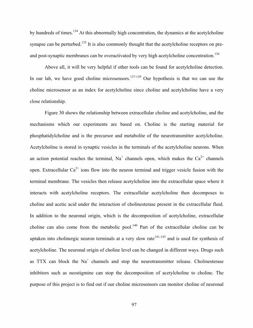
by hundreds of times.134 At this abnormally high concentration, the dynamics at the acetylcholine
synapse can be perturbed.135 It is also commonly thought that the acetylcholine receptors on pre-
and post-synaptic membranes can be overactivated by very high acetylcholine concentration.136
Above all, it will be very helpful if other tools can be found for acetylcholine detection.
In our lab, we have good choline microsensors.137-139 Our hypothesis is that we can use the
choline microsensor as an index for acetylcholine since choline and acetylcholine have a very
close relationship.
Figure 30 shows the relationship between extracellular choline and acetylcholine, and the
mechanisms which our experiments are based on. Choline is the starting material for
phosphatidylcholine and is the precursor and metabolite of the neurotransmitter acetylcholine.
Acetylcholine is stored in synaptic vesicles in the terminals of the acetylcholine neurons. When
an action potential reaches the terminal, Na+ channels open, which makes the Ca2+ channels
open. Extracellular Ca2+ ions flow into the neuron terminal and trigger vesicle fusion with the
terminal membrane. The vesicles then release acetylcholine into the extracellular space where it
interacts with acetylcholine receptors. The extracellular acetylcholine then decomposes to
choline and acetic acid under the interaction of cholinesterase present in the extracellular fluid.
In addition to the neuronal origin, which is the decomposition of acetylcholine, extracellular
choline can also come from the metabolic pool.140 Part of the extracellular choline can be
uptaken into cholinergic neuron terminals at a very slow rate141-143 and is used for synthesis of
acetylcholine. The neuronal origin of choline level can be changed in different ways. Drugs such
as TTX can block the Na+ channels and stop the neurotransmitter release. Cholinesterase
inhibitors such as neostigmine can stop the decomposition of acetylcholine to choline. The
purpose of this project is to find out if our choline microsensors can monitor choline of neuronal
97

98
origin, the decomposition of acetylcholine, and thus further study on acetylcholine. We need to
design the experiments very carefully to confirm our idea.
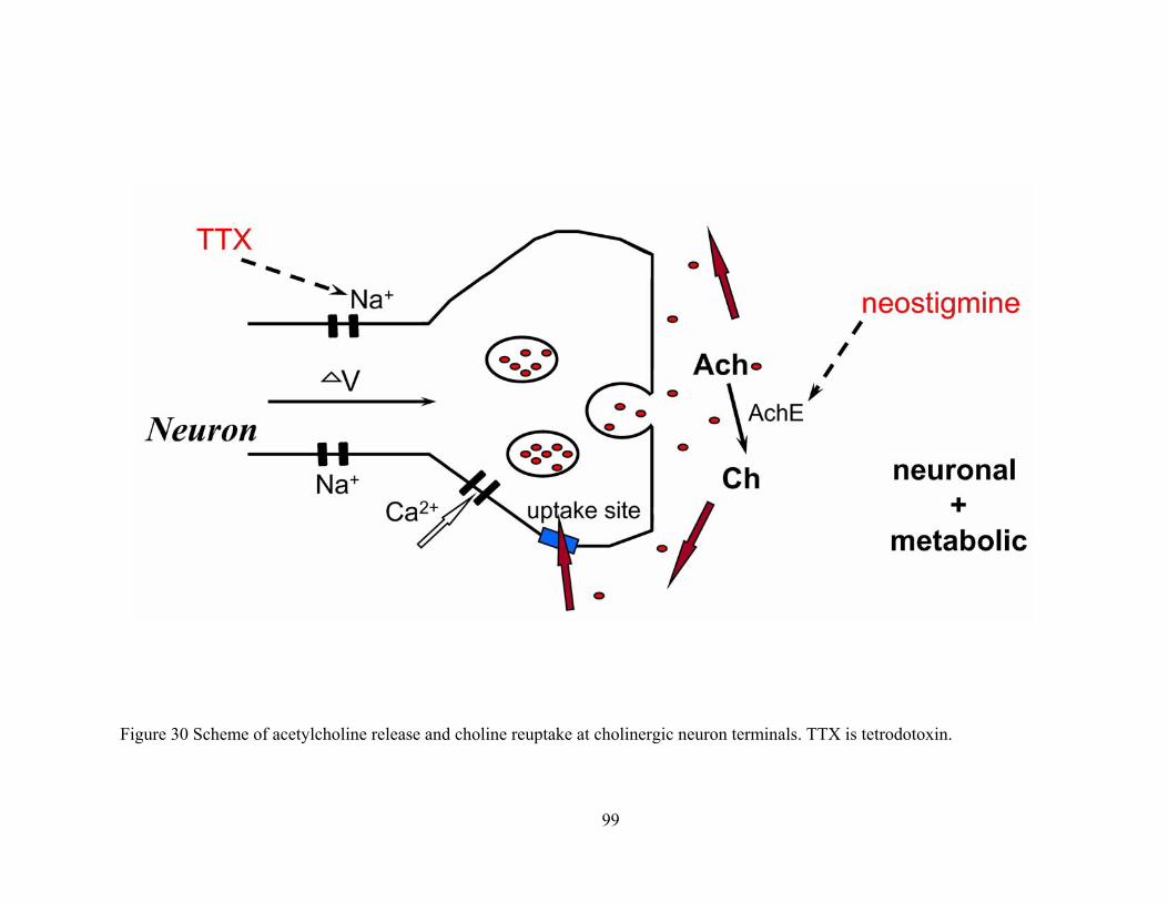
99
Figure 30 Scheme of acetylcholine release and choline reuptake at cholinergic neuron terminals. TTX is tetrodotoxin.
The following paragraphs provide some basic principles about how our choline oxidase
and glucose oxidase modified microsensors operate.
Microelectrodes provide a successful tool for monitoring electroactive neurotransmitters
and their metabolites in the brain.144,145 The small size of microelectrodes (~10,000 smaller
compared to common microdialysis probes) causes less damage to the brain tissue than
microdialysis probes. The disadvantage of microelectrodes is that they can not measure many
non-eletroactive neurotransmitters. Enzyme modified microelectrodes have been a topic of
interest for a long time due to their many properties, such as sensitivity towards various non-
electroactive substrates, selectivity over ascorbate, miniaturization etc.146 They are particularly
suitable for real time in vivo measurement.
Choline microsensors have long been studied in our lab. Figure 31 shows how the choline
microsensor operates. The microsensors were made according the procedures modified from the
traditional procedure in our lab. The microsensor is based upon a bienzyme mechanism. A
carbon fiber was used as the substrate microelectrode. Choline oxidase and horseradish
peroxidase (HRP) were immobilized in the crosslinked redox polymer matrix. Upon catalysis by
immobilized choline oxidase, choline reacts with oxygen in the extracellular fluid to produce
betaine and hydrogen peroxide. HRP is then oxidized by hydrogen peroxide. Then the oxidized
form of HRP is reduced by the mediator, OsII. Finally, the oxidized OsIII is reduced by the
substrate electrode. The redox centers that are far from the electrode surface transfer electrons by
an electron self-exchange reaction between neighboring redox centers, a process called electron
hopping.147,148 Redox mediator, OsII/III, was used because it can work at the potential of –100
mV vs. Ag/AgCl (1.0 M KCl) reference electrode. Compared to the more extreme potentials
needed for direct measurement of hydrogen peroxide production or oxygen consumption,149,150
100
Figure 31. (a) Schematic representation of the sequential reactions that occurred at the choline bienzyme microsensor. Structures of (b) the redox polymer and (c) the crosslinker that were used to immobilize the enzymes onto the carbon fiber microelectrode surface.
101
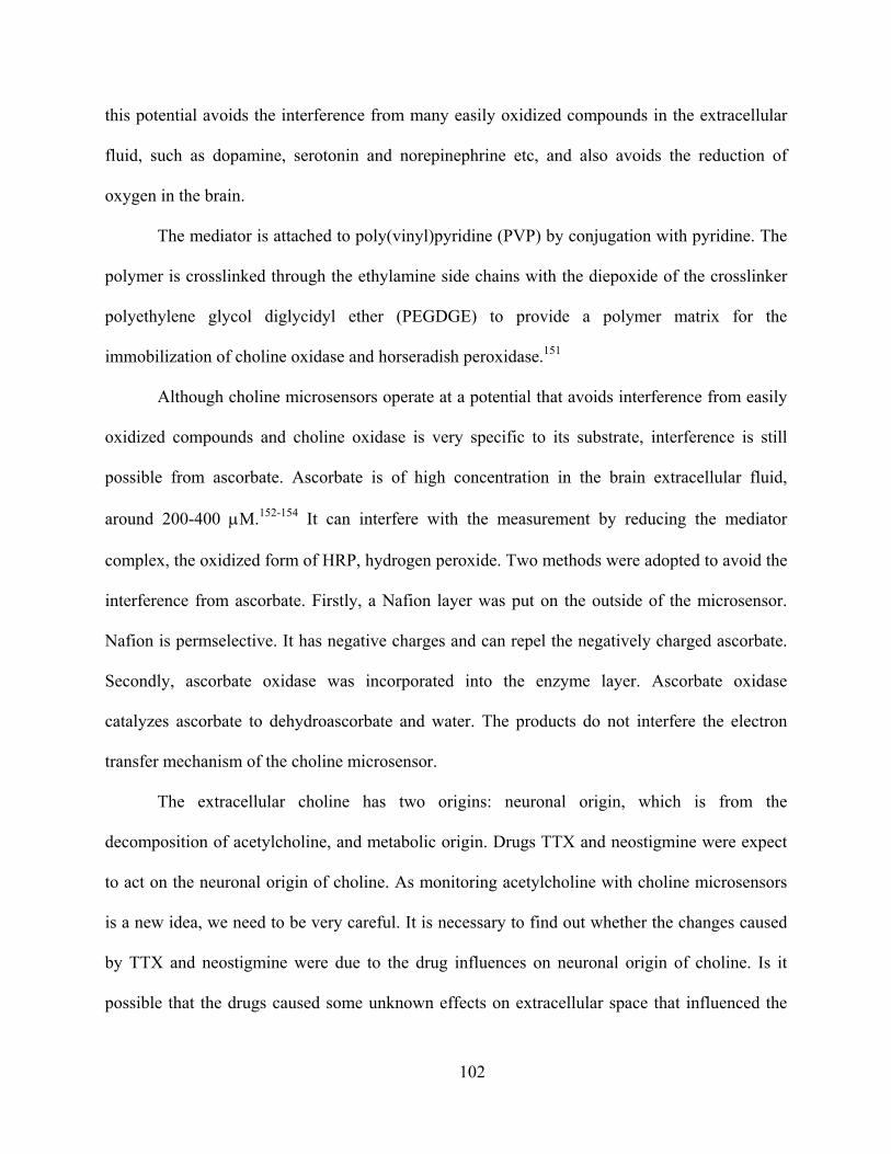
this potential avoids the interference from many easily oxidized compounds in the extracellular
fluid, such as dopamine, serotonin and norepinephrine etc, and also avoids the reduction of
oxygen in the brain.
The mediator is attached to poly(vinyl)pyridine (PVP) by conjugation with pyridine. The
polymer is crosslinked through the ethylamine side chains with the diepoxide of the crosslinker
polyethylene glycol diglycidyl ether (PEGDGE) to provide a polymer matrix for the
immobilization of choline oxidase and horseradish peroxidase.151
Although choline microsensors operate at a potential that avoids interference from easily
oxidized compounds and choline oxidase is very specific to its substrate, interference is still
possible from ascorbate. Ascorbate is of high concentration in the brain extracellular fluid,
around 200-400 μM.152-154 It can interfere with the measurement by reducing the mediator
complex, the oxidized form of HRP, hydrogen peroxide. Two methods were adopted to avoid the
interference from ascorbate. Firstly, a Nafion layer was put on the outside of the microsensor.
Nafion is permselective. It has negative charges and can repel the negatively charged ascorbate.
Secondly, ascorbate oxidase was incorporated into the enzyme layer. Ascorbate oxidase
catalyzes ascorbate to dehydroascorbate and water. The products do not interfere the electron
transfer mechanism of the choline microsensor.
The extracellular choline has two origins: neuronal origin, which is from the
decomposition of acetylcholine, and metabolic origin. Drugs TTX and neostigmine were expect
to act on the neuronal origin of choline. As monitoring acetylcholine with choline microsensors
is a new idea, we need to be very careful. It is necessary to find out whether the changes caused
by TTX and neostigmine were due to the drug influences on neuronal origin of choline. Is it
possible that the drugs caused some unknown effects on extracellular space that influenced the
102
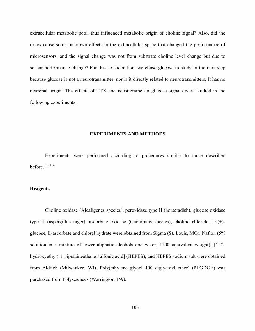
extracellular metabolic pool, thus influenced metabolic origin of choline signal? Also, did the
drugs cause some unknown effects in the extracellular space that changed the performance of
microsensors, and the signal change was not from substrate choline level change but due to
sensor performance change? For this consideration, we chose glucose to study in the next step
because glucose is not a neurotransmitter, nor is it directly related to neurotransmitters. It has no
neuronal origin. The effects of TTX and neostigmine on glucose signals were studied in the
following experiments.
EXPERIMENTS AND METHODS
Experiments were performed according to procedures similar to those described
before.155,156
Reagents
Choline oxidase (Alcaligenes species), peroxidase type II (horseradish), glucose oxidase
type II (aspergillus niger), ascorbate oxidase (Cucurbitas species), choline chloride, D-(+)-
glucose, L-ascorbate and chloral hydrate were obtained from Sigma (St. Louis, MO). Nafion (5%
solution in a mixture of lower aliphatic alcohols and water, 1100 equivalent weight), [4-(2-
hydroxyethyl)-1-piprazineethane-sulfonic acid] (HEPES), and HEPES sodium salt were obtained
from Aldrich (Milwaukee, WI). Poly(ethylene glycol 400 diglycidyl ether) (PEGDGE) was
purchased from Polysciences (Warrington, PA).
103
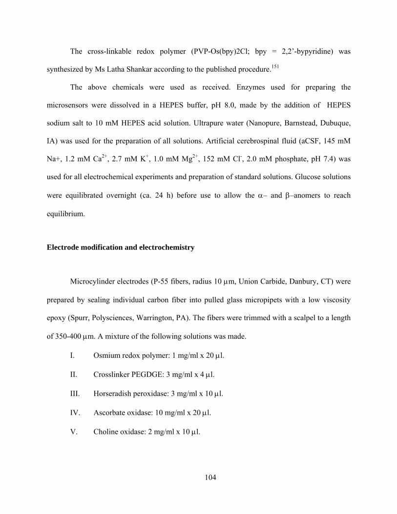
The cross-linkable redox polymer (PVP-Os(bpy)2Cl; bpy = 2,2’-bypyridine) was
synthesized by Ms Latha Shankar according to the published procedure.151
The above chemicals were used as received. Enzymes used for preparing the
microsensors were dissolved in a HEPES buffer, pH 8.0, made by the addition of HEPES
sodium salt to 10 mM HEPES acid solution. Ultrapure water (Nanopure, Barnstead, Dubuque,
IA) was used for the preparation of all solutions. Artificial cerebrospinal fluid (aCSF, 145 mM
Na+, 1.2 mM Ca2+, 2.7 mM K+, 1.0 mM Mg2+, 152 mM Cl-, 2.0 mM phosphate, pH 7.4) was
used for all electrochemical experiments and preparation of standard solutions. Glucose solutions
were equilibrated overnight (ca. 24 h) before use to allow the α– and β–anomers to reach
equilibrium.
Electrode modification and electrochemistry
Microcylinder electrodes (P-55 fibers, radius 10 μm, Union Carbide, Danbury, CT) were
prepared by sealing individual carbon fiber into pulled glass micropipets with a low viscosity
epoxy (Spurr, Polysciences, Warrington, PA). The fibers were trimmed with a scalpel to a length
of 350-400 μm. A mixture of the following solutions was made.
I. Osmium redox polymer: 1 mg/ml x 20 μl.
II. Crosslinker PEGDGE: 3 mg/ml x 4 μl.
III. Horseradish peroxidase: 3 mg/ml x 10 μl.
IV. Ascorbate oxidase: 10 mg/ml x 20 μl.
V. Choline oxidase: 2 mg/ml x 10 μl.
104
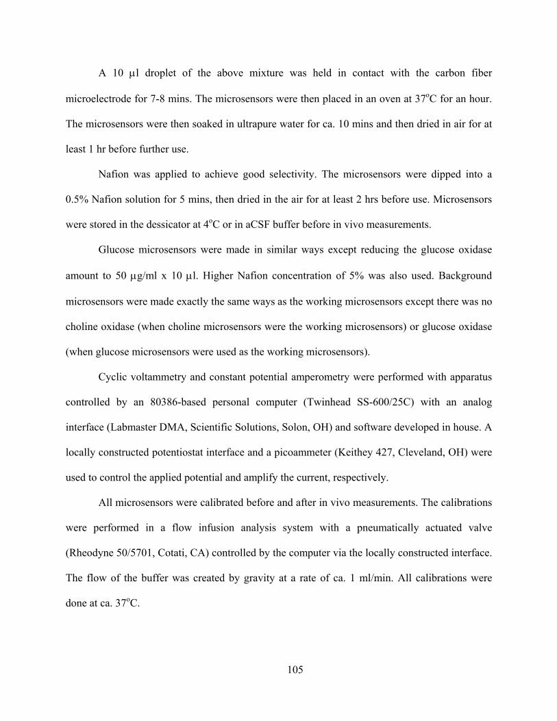
A 10 μl droplet of the above mixture was held in contact with the carbon fiber
microelectrode for 7-8 mins. The microsensors were then placed in an oven at 37oC for an hour.
The microsensors were then soaked in ultrapure water for ca. 10 mins and then dried in air for at
least 1 hr before further use.
Nafion was applied to achieve good selectivity. The microsensors were dipped into a
0.5% Nafion solution for 5 mins, then dried in the air for at least 2 hrs before use. Microsensors
were stored in the dessicator at 4oC or in aCSF buffer before in vivo measurements.
Glucose microsensors were made in similar ways except reducing the glucose oxidase
amount to 50 μg/ml x 10 μl. Higher Nafion concentration of 5% was also used. Background
microsensors were made exactly the same ways as the working microsensors except there was no
choline oxidase (when choline microsensors were the working microsensors) or glucose oxidase
(when glucose microsensors were used as the working microsensors).
Cyclic voltammetry and constant potential amperometry were performed with apparatus
controlled by an 80386-based personal computer (Twinhead SS-600/25C) with an analog
interface (Labmaster DMA, Scientific Solutions, Solon, OH) and software developed in house. A
locally constructed potentiostat interface and a picoammeter (Keithey 427, Cleveland, OH) were
used to control the applied potential and amplify the current, respectively.
All microsensors were calibrated before and after in vivo measurements. The calibrations
were performed in a flow infusion analysis system with a pneumatically actuated valve
(Rheodyne 50/5701, Cotati, CA) controlled by the computer via the locally constructed interface.
The flow of the buffer was created by gravity at a rate of ca. 1 ml/min. All calibrations were
done at ca. 37oC.
105
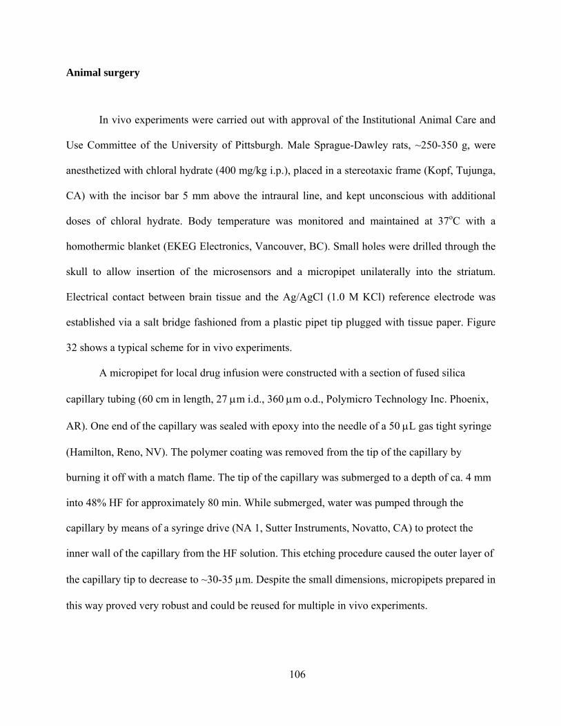
106
Animal surgery
In vivo experiments were carried out with approval of the Institutional Animal Care and
Use Committee of the University of Pittsburgh. Male Sprague-Dawley rats, ~250-350 g, were
anesthetized with chloral hydrate (400 mg/kg i.p.), placed in a stereotaxic frame (Kopf, Tujunga,
CA) with the incisor bar 5 mm above the intraural line, and kept unconscious with additional
doses of chloral hydrate. Body temperature was monitored and maintained at 37oC with a
homothermic blanket (EKEG Electronics, Vancouver, BC). Small holes were drilled through the
skull to allow insertion of the microsensors and a micropipet unilaterally into the striatum.
Electrical contact between brain tissue and the Ag/AgCl (1.0 M KCl) reference electrode was
established via a salt bridge fashioned from a plastic pipet tip plugged with tissue paper. Figure
32 shows a typical scheme for in vivo experiments.
A micropipet for local drug infusion were constructed with a section of fused silica
capillary tubing (60 cm in length, 27 μm i.d., 360 μm o.d., Polymicro Technology Inc. Phoenix,
AR). One end of the capillary was sealed with epoxy into the needle of a 50 μL gas tight syringe
(Hamilton, Reno, NV). The polymer coating was removed from the tip of the capillary by
burning it off with a match flame. The tip of the capillary was submerged to a depth of ca. 4 mm
into 48% HF for approximately 80 min. While submerged, water was pumped through the
capillary by means of a syringe drive (NA 1, Sutter Instruments, Novatto, CA) to protect the
inner wall of the capillary from the HF solution. This etching procedure caused the outer layer of
the capillary tip to decrease to ~30-35 μm. Despite the small dimensions, micropipets prepared in
this way proved very robust and could be reused for multiple in vivo experiments.
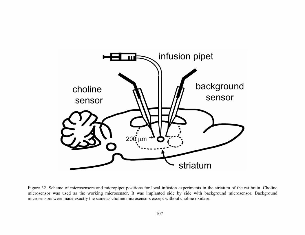
107
Figure 32. Scheme of microsensors and micropipet positions for local infusion experiments in the striatum of the rat brain. Choline microsensor was used as the working microsensor. It was implanted side by side with background microsensor. Background microsensors were made exactly the same as choline microsensors except without choline oxidase.
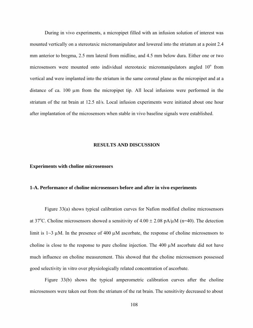
During in vivo experiments, a micropipet filled with an infusion solution of interest was
mounted vertically on a stereotaxic micromanipulator and lowered into the striatum at a point 2.4
mm anterior to bregma, 2.5 mm lateral from midline, and 4.5 mm below dura. Either one or two
microsensors were mounted onto individual stereotaxic micromanipulators angled 10o from
vertical and were implanted into the striatum in the same coronal plane as the micropipet and at a
distance of ca. 100 μm from the micropipet tip. All local infusions were performed in the
striatum of the rat brain at 12.5 nl/s. Local infusion experiments were initiated about one hour
after implantation of the microsensors when stable in vivo baseline signals were established.
RESULTS AND DISCUSSION
Experiments with choline microsensors
1-A. Performance of choline microsensors before and after in vivo experiments
Figure 33(a) shows typical calibration curves for Nafion modified choline microsensors
at 37oC. Choline microsensors showed a sensitivity of 4.00 ± 2.08 pA/μM (n=40). The detection
limit is 1~3 μM. In the presence of 400 μM ascorbate, the response of choline microsensors to
choline is close to the response to pure choline injection. The 400 μM ascorbate did not have
much influence on choline measurement. This showed that the choline microsensors possessed
good selectivity in vitro over physiologically related concentration of ascorbate.
Figure 33(b) shows the typical amperometric calibration curves after the choline
microsensors were taken out from the striatum of the rat brain. The sensitivity decreased to about
108
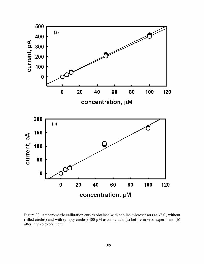
Figure 33. Amperometric calibration curves obtained with choline microsensors at 37oC, without (filled circles) and with (empty circles) 400 µM ascorbic acid (a) before in vivo experiment. (b) after in vivo experiment.
109
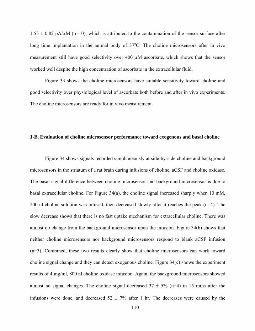
110
1.55 ± 0.82 pA/μM (n=10), which is attributed to the contamination of the sensor surface after
long time implantation in the animal body of 37oC. The choline microsensors after in vivo
measurement still have good selectivity over 400 μM ascorbate, which shows that the sensor
worked well despite the high concentration of ascorbate in the extracellular fluid.
Figure 33 shows the choline microsensors have suitable sensitivity toward choline and
good selectivity over physiological level of ascorbate both before and after in vivo experiments.
The choline microsensors are ready for in vivo measurement.
1-B. Evaluation of choline microsensor performance toward exogenous and basal choline
Figure 34 shows signals recorded simultaneously at side-by-side choline and background
microsensors in the striatum of a rat brain during infusions of choline, aCSF and choline oxidase.
The basal signal difference between choline microsensor and background microsensor is due to
basal extracellular choline. For Figure 34(a), the choline signal increased sharply when 10 mM,
200 nl choline solution was infused, then decreased slowly after it reaches the peak (n=4). The
slow decrease shows that there is no fast uptake mechanism for extracellular choline. There was
almost no change from the background microsensor upon the infusion. Figure 34(b) shows that
neither choline microsensors nor background microsensors respond to blank aCSF infusion
(n=3). Combined, these two results clearly show that choline microsensors can work toward
choline signal change and they can detect exogenous choline. Figure 34(c) shows the experiment
results of 4 mg/ml, 800 nl choline oxidase infusion. Again, the background microsensors showed
almost no signal changes. The choline signal decreased 37 ± 5% (n=4) in 15 mins after the
infusions were done, and decreased 52 ± 7% after 1 hr. The decreases were caused by the
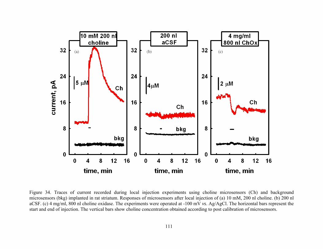
111
Figure 34. Traces of current recorded during local injection experiments using choline microsensors (Ch) and background microsensors (bkg) implanted in rat striatum. Responses of microsensors after local injection of (a) 10 mM, 200 nl choline. (b) 200 nl aCSF. (c) 4 mg/ml, 800 nl choline oxidase. The experiments were operated at -100 mV vs. Ag/AgCl. The horizontal bars represent the start and end of injection. The vertical bars show choline concentration obtained according to post calibration of microsensors.
consumption of extracellular choline by infused choline oxidase. The effect of infused choline
oxidase may be stronger after 1 hr. as we can see by comparing the decreasing values. This
experiment showed that choline microsensors can also detect basal extracellular choline. From
the above choline solution infusion experiments and choline oxidase infusion experiments, the
recorded signals did show that the choline microsensors we made could detect the choline signal
changes both from exogenous and endogenous choline level changes.
1-C. Effect of tetrodotoxin on choline signals
Tetrodotoxin (TTX) is a very common drug to study the neuronal origin of a
substance.157,158 It works by blocking the Na+ channels on the neuron terminals, stopping the
following flow-in of Ca2+ ions into the neuron terminals, stopping the fusion of vesicles with the
neuronal membrane following Ca2+ rush-in, thus stopping neurotransmitter release. For
acetylcholine, if its release from cholinergic terminals is stopped by TTX, the extracellular
acetylcholine level decreases. So will extracellular choline signal decrease correspondingly since
part of it comes from the decomposition of extracellular acetylcholine? Can our choline
microsensors detect this change?
Figure 35 shows the recorded signals from choline microsensor and the control
microsensor implanted side by side with the infusion of 100 μM, 200 nl TTX. There was no
signal change from the control microsensor. The choline signal decreased by 21 ± 7% (n=5). The
decrease of choline signal can possibly be attributed to the neuronal origin of choline, the
extracellular acetylcholine decomposition. Post calibration data (Figure 36) were obtained by
testing the responses of choline microsensor to choline and the mixture of choline and 100 μM
112
Figure 35. Traces of current recorded during local infusion of 100 µM, 200 nl tetrodotoxin (TTX) with choline microsensor (Ch) and background microsensor (bkg) implanted side by side in tha rat striatum. The experiments were operated at -100 mV vs. Ag/AgCl. The horizontal bar represents the start and end of infusion. The vertical bar represents choline concentration obtained according to the post calibration of microsensors.
113
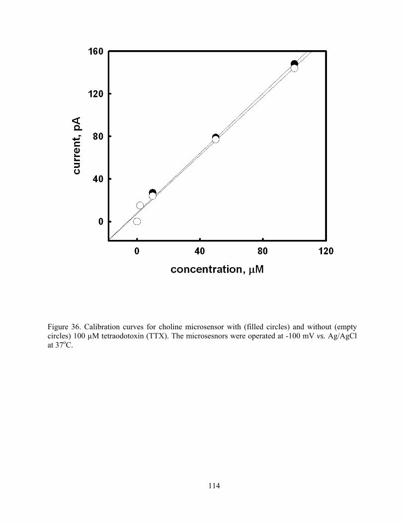
Figure 36. Calibration curves for choline microsensor with (filled circles) and without (empty circles) 100 µM tetraodotoxin (TTX). The microsesnors were operated at -100 mV vs. Ag/AgCl at 37oC.
114
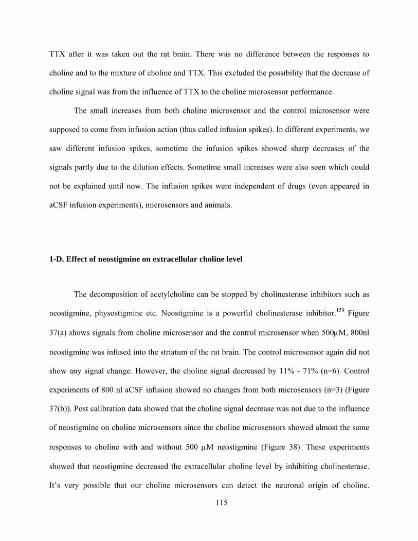
115
TTX after it was taken out the rat brain. There was no difference between the responses to
choline and to the mixture of choline and TTX. This excluded the possibility that the decrease of
choline signal was from the influence of TTX to the choline microsensor performance.
The small increases from both choline microsensor and the control microsensor were
supposed to come from infusion action (thus called infusion spikes). In different experiments, we
saw different infusion spikes, sometime the infusion spikes showed sharp decreases of the
signals partly due to the dilution effects. Sometime small increases were also seen which could
not be explained until now. The infusion spikes were independent of drugs (even appeared in
aCSF infusion experiments), microsensors and animals.
1-D. Effect of neostigmine on extracellular choline level
The decomposition of acetylcholine can be stopped by cholinesterase inhibitors such as
neostigmine, physostigmine etc. Neostigmine is a powerful cholinesterase inhibitor.159 Figure
37(a) shows signals from choline microsensor and the control microsensor when 500μM, 800nl
neostigmine was infused into the striatum of the rat brain. The control microsensor again did not
show any signal change. However, the choline signal decreased by 11% - 71% (n=6). Control
experiments of 800 nl aCSF infusion showed no changes from both microsensors (n=3) (Figure
37(b)). Post calibration data showed that the choline signal decrease was not due to the influence
of neostigmine on choline microsensors since the choline microsensors showed almost the same
responses to choline with and without 500 μM neostigmine (Figure 38). These experiments
showed that neostigmine decreased the extracellular choline level by inhibiting cholinesterase.
It’s very possible that our choline microsensors can detect the neuronal origin of choline.
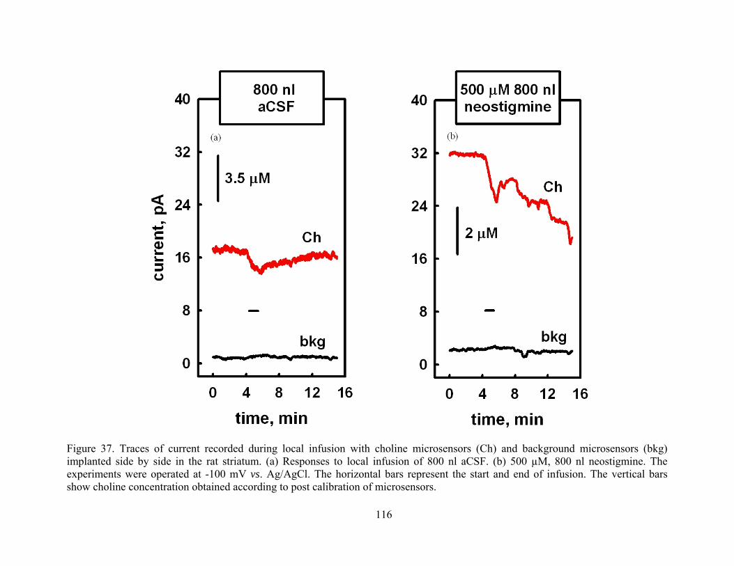
116
Figure 37. Traces of current recorded during local infusion with choline microsensors (Ch) and background microsensors (bkg) implanted side by side in the rat striatum. (a) Responses to local infusion of 800 nl aCSF. (b) 500 µM, 800 nl neostigmine. The experiments were operated at -100 mV vs. Ag/AgCl. The horizontal bars represent the start and end of infusion. The vertical bars show choline concentration obtained according to post calibration of microsensors.
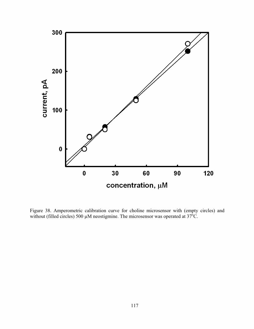
Figure 38. Amperometric calibration curve for choline microsensor with (empty circles) and without (filled circles) 500 µM neostigmine. The microsensor was operated at 37oC.
117
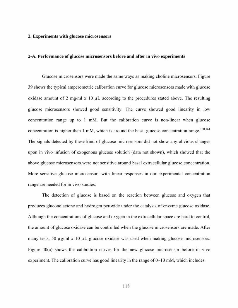
2. Experiments with glucose microsensors
2-A. Performance of glucose microsensors before and after in vivo experiments
Glucose microsensors were made the same ways as making choline microsensors. Figure
39 shows the typical amperometric calibration curve for glucose microsensors made with glucose
oxidase amount of 2 mg/ml x 10 μL according to the procedures stated above. The resulting
glucose microsensors showed good sensitivity. The curve showed good linearity in low
concentration range up to 1 mM. But the calibration curve is non-linear when glucose
concentration is higher than 1 mM, which is around the basal glucose concentration range.160,161
The signals detected by these kind of glucose microsensors did not show any obvious changes
upon in vivo infusion of exogenous glucose solution (data not shown), which showed that the
above glucose microsensors were not sensitive around basal extracellular glucose concentration.
More sensitive glucose microsensors with linear responses in our experimental concentration
range are needed for in vivo studies.
The detection of glucose is based on the reaction between glucose and oxygen that
produces gluconolactone and hydrogen peroxide under the catalysis of enzyme glucose oxidase.
Although the concentrations of glucose and oxygen in the extracellular space are hard to control,
the amount of glucose oxidase can be controlled when the glucose microsensors are made. After
many tests, 50 μg/ml x 10 μL glucose oxidase was used when making glucose microsensors.
Figure 40(a) shows the calibration curves for the new glucose microsensor before in vivo
experiment. The calibration curve has good linearity in the range of 0~10 mM, which includes
118
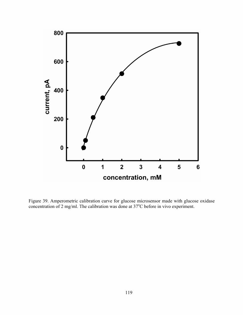
Figure 39. Amperometric calibration curve for glucose microsensor made with glucose oxidase concentration of 2 mg/ml. The calibration was done at 37oC before in vivo experiment.
119
Figure 40. Amperometric calibration curves for glucose microsensors made with glucose oxidase concentration of 75 µg/ml. The calibration wre made with (empty circles) and without (filled circles) 400 µM ascorbic acid at 37oC (a) before in vivo experiment. (b) after in vivo experiment.
120
121
possible basal extracellular glucose concentration range. The sensors have suitable sensitivity of
36.31 ± 22.30 pA/mM (n=15), the detection limit of ~100~200 μM. They also showed good
selectivity over 400 μM ascorbate. The sensitivity of the new glucose microsensors did not
change a lot after the in vivo experiment (Figure 40(b)). The glucose microsensors remained
well selective over 400 μM ascorbate after in vivo experiments. The new glucose microsensors
are ready for in vivo measurements now.
2-B. Evaluation of glucose microsensor performance toward exogenous and basal glucose
Firstly, it is an important thing to check if glucose microsensors can detect the
extracellular glucose signal change and basal glucose signal or not. The glucose infusion and
glucose oxidase infusion experiments were designed to test the in vivo performance of glucose
microsensors. Figure 41 showed the signals recorded when glucose microsensors and the control
microsensors were implanted side by side, and 200 nl aCSF, 1M 200 nl glucose, or 4 mg/ml 800
nl glucose oxidase were infused into the rat striatum. The glucose microsensors did not respond
to the aCSF infusion (n=4) (Figure 41(a)). When 1 M 200 nl glucose solution was infused,
glucose signal increased sharply and then recovered slowly, which corresponds to clearance by
diffusion (n=6) (Figure 41(b)). This shows that glucose microsensors detect extracellular glucose
change caused by exogenous glucose infusion. When 4 mg/ml, 800 nl glucose oxidase solution
was infused (Figure 41(c)), the basal glucose signal decreased. The basal current detected by
glucose microsensor was from the basal extracellular glucose. This showed that our glucose
microsensors could detect basal glucose level.
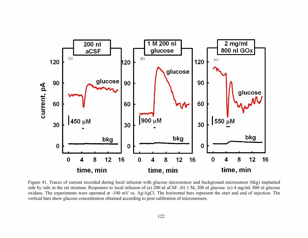
122
Figure 41. Traces of current recorded during local infusion with glucose microsensor and background microsensor (bkg) implanted side by side in the rat striatum. Responses to local infusion of (a) 200 nl aCSF. (b) 1 M, 200 nl glucose. (c) 4 mg/ml, 800 nl glucose oxidase. The experiments were operated at -100 mV vs. Ag/AgCl. The horizontal bars represent the start and end of injection. The vertical bars show glucose concentration obtained according to post calibration of microsensors.
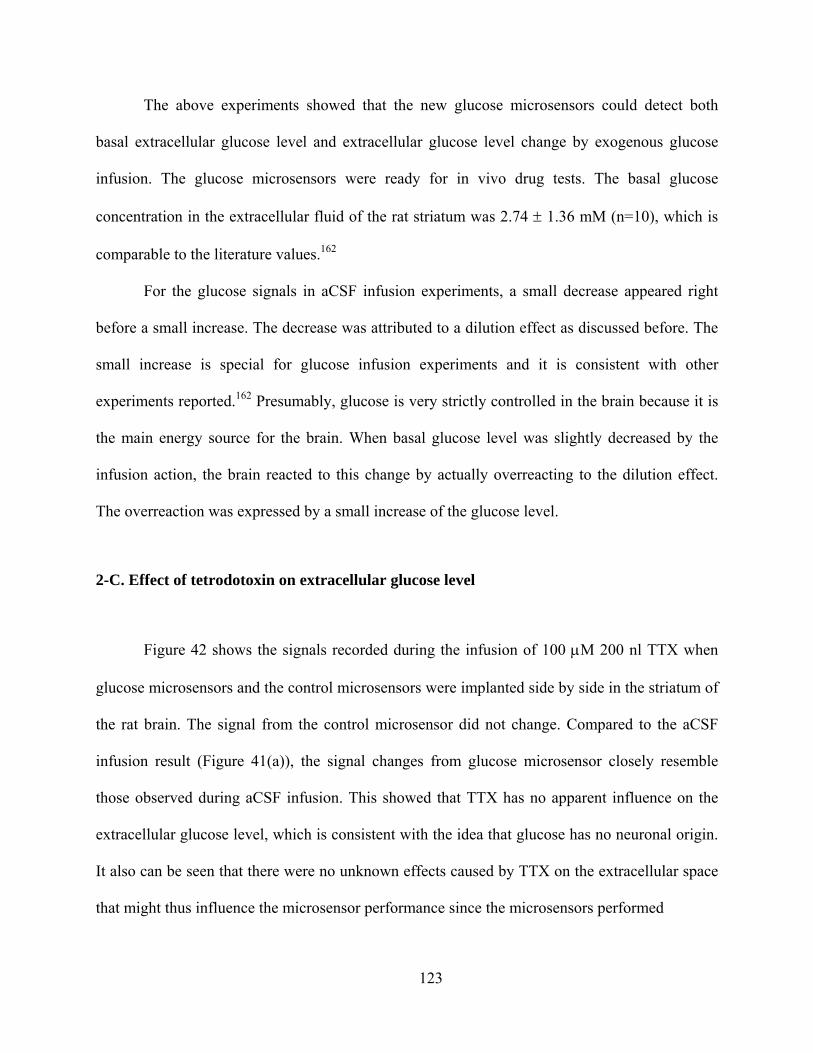
The above experiments showed that the new glucose microsensors could detect both
basal extracellular glucose level and extracellular glucose level change by exogenous glucose
infusion. The glucose microsensors were ready for in vivo drug tests. The basal glucose
concentration in the extracellular fluid of the rat striatum was 2.74 ± 1.36 mM (n=10), which is
comparable to the literature values.162
For the glucose signals in aCSF infusion experiments, a small decrease appeared right
before a small increase. The decrease was attributed to a dilution effect as discussed before. The
small increase is special for glucose infusion experiments and it is consistent with other
experiments reported.162 Presumably, glucose is very strictly controlled in the brain because it is
the main energy source for the brain. When basal glucose level was slightly decreased by the
infusion action, the brain reacted to this change by actually overreacting to the dilution effect.
The overreaction was expressed by a small increase of the glucose level.
2-C. Effect of tetrodotoxin on extracellular glucose level
Figure 42 shows the signals recorded during the infusion of 100 μM 200 nl TTX when
glucose microsensors and the control microsensors were implanted side by side in the striatum of
the rat brain. The signal from the control microsensor did not change. Compared to the aCSF
infusion result (Figure 41(a)), the signal changes from glucose microsensor closely resemble
those observed during aCSF infusion. This showed that TTX has no apparent influence on the
extracellular glucose level, which is consistent with the idea that glucose has no neuronal origin.
It also can be seen that there were no unknown effects caused by TTX on the extracellular space
that might thus influence the microsensor performance since the microsensors performed
123
Figure 42. Traces of current recorded during local infusion of 100 µM, 200 nl TTX with glucose microsensor and background microsensor (bkg). The experiments were operated at -100 mV vs. Ag/AgCl. The horizontal bar represents the start and end of injection. The vertical bar shows glucose concentration obtained according to post calibration of microsensors.
124
similarly during both TTX and aCSF infusions. Considering that TTX infusion decreased
extracellular choline level, we can conclude that the decrease of extracellular choline level was
coming from the neuronal origin of choline, which is the decomposition of extracellular
acetylcholine. TTX has no direct influence on glucose microsensors performance as shown by
Figure 43.
2-D. Effect of neostigmine on extracellular glucose level
To find out if neostigmine caused any unknown influence on extracellular space, thus
influenced the microsensor performance or decreased the metabolic origin of choline instead of
neuronal origin of choline, neostigmine infusion experiments were done with glucose
microsensors and the control microsensors implanted side by side in the rat striatum. Figure 44
shows the experiments with the infusion of (a) 800 nl aCSF (n=4), (b) 500 μM 800 nl
neostigmine (n=4). The infusion of neostigmine produced similar effect to the infusion of buffer
aCSF. Neostigmine did not influence the glucose level or the microsensor performance.
Considering the result that neostigmine infusion decreased extracellular choline level, this
proved that the extracellular choline signal decrease caused by neostigmine was from the
inhibition of enzyme cholinesterase and thus stop the decomposition of acetylcholine to choline.
The decreases detected by choline microsensors when neostigmine was infused were from the
neuronal origin of choline. Neostigmine had no obvious influence on metabolic origin of choline,
nor did it change microsensor performance indirectly by influencing the extracellular space. Post
calibration data showed that neostigmine did not have direct influence on the performance of
glucose microsensors.(Figure 45)
125
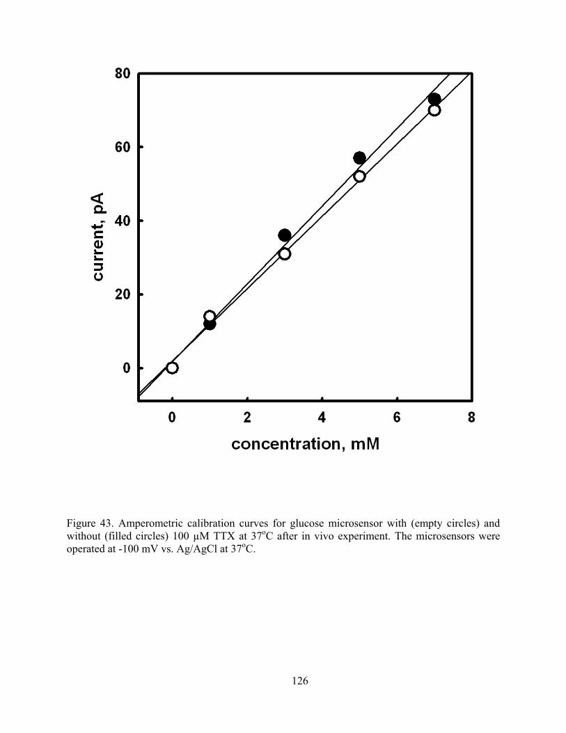
Figure 43. Amperometric calibration curves for glucose microsensor with (empty circles) and without (filled circles) 100 µM TTX at 37oC after in vivo experiment. The microsensors were operated at -100 mV vs. Ag/AgCl at 37oC.
126
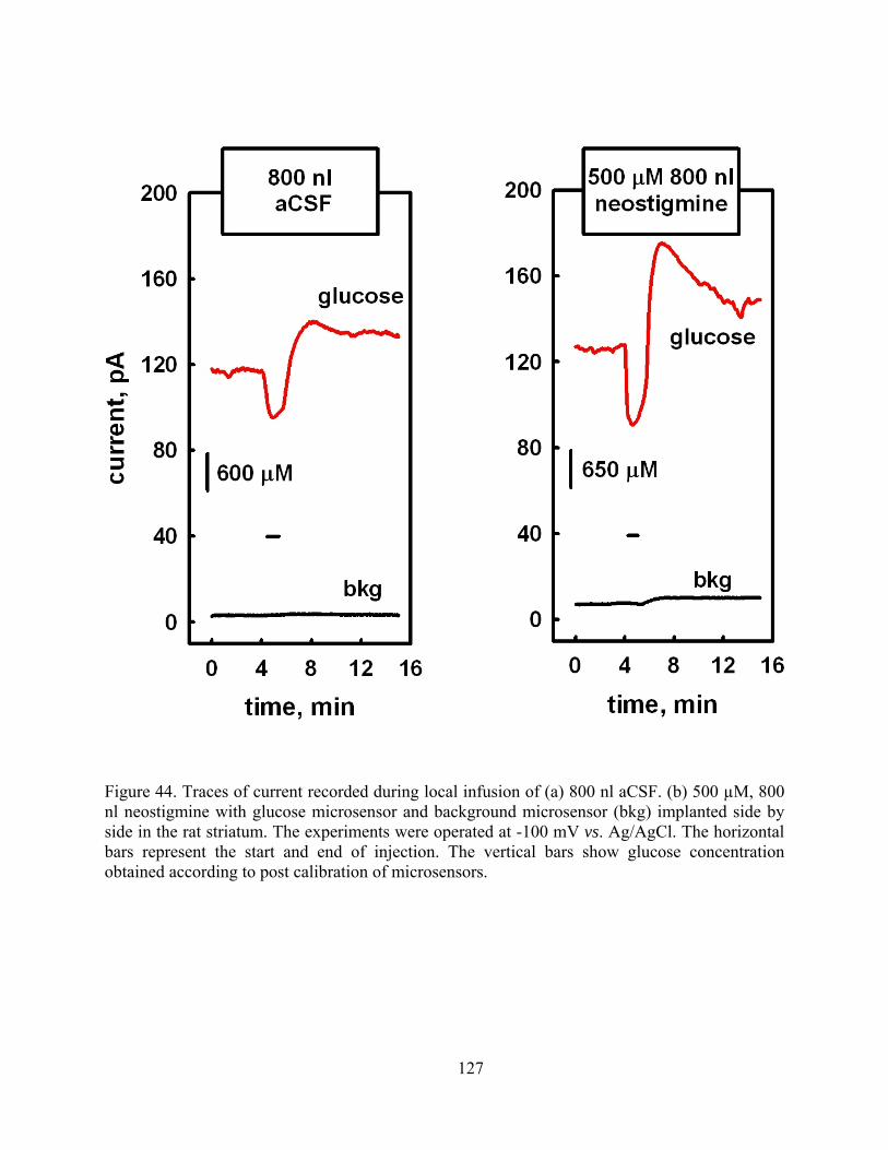
Figure 44. Traces of current recorded during local infusion of (a) 800 nl aCSF. (b) 500 µM, 800 nl neostigmine with glucose microsensor and background microsensor (bkg) implanted side by side in the rat striatum. The experiments were operated at -100 mV vs. Ag/AgCl. The horizontal bars represent the start and end of injection. The vertical bars show glucose concentration obtained according to post calibration of microsensors.
127
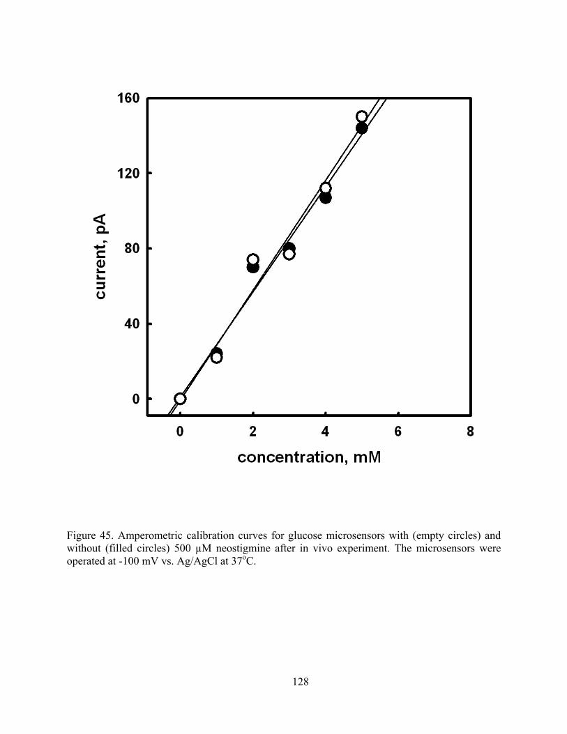
Figure 45. Amperometric calibration curves for glucose microsensors with (empty circles) and without (filled circles) 500 µM neostigmine after in vivo experiment. The microsensors were operated at -100 mV vs. Ag/AgCl at 37oC.
128
CONCLUSION
The choline microsensors developed in this lab could detect choline signal changes both
from exogenous choline and basal extracellular choline. Glucose microsensors responded to
exogenous and basal glucose level changes. Enzyme modified microelectrode is a feasible tool
for in vivo detection. By stopping neurotransmitter release with TTX, extracellular choline signal
decreased. TTX had no effect on extracellular glucose signal. Neostigmine decreased
extracellular choline level by inhibiting cholinesterase and stopping the decomposition of
acetylcholine to choline. Neostigmine had no influence on extracellular glucose level. Glucose
control experiments excluded two possibilities: 1. TTX and neostigmine changed metabolic
origin of choline. 2. TTX and neostigmine changed extracellular space and thus changed
microsensor performance in vivo. The above results showed that the decreases of choline signals
under TTX and neostigmine infusions were due to the decreases of neuronal origin of choline.
We conclude that choline microsensors can detect neuronal origin of choline. This is the first
demonstration that extracellular choline has neuronal origin. We discovered that it is possible to
index neurotransmitter acetylcholine by our choline microsensors. We expect more contribution
to cholinergic study with choline microsensors.
129
FUTURE DIRECTION
The relationship between cholinergic systems and dopaminergic systems has long been a
topic since it was first found in 1960s. Many diseases such as Parkinson’s disease, Huntington’s
disease are related to the interaction between dopaminergic systems and cholinergic
systems.163,164 It was found that some totally different drugs, such as cholinergic muscarinic
receptor antagonists, which inhibit the cholinergic systems, and dopaminergic agonists, which
stimulate dopaminergic systems, can both relieve the symptoms of Parkinson’s disease.165,166 It
was hypothesized that there was some relationship between cholinergic systems and
dopaminergic systems. It was supposed that these two neurotransmission systems had opposite
functions in the brain and there was a balance between them. Later research confirmed the
relationship between cholinergic systems and dopaminergic systems. People found that
dopaminergic receptor agonists, which stimulate dopaminergic systems, can decrease the
striatum acetylcholine level and dopaminergic antagonists, which inhibit dopaminergic systems,
can increase striatum acetylcholine level.167,168 Further research found that dopaminergic systems
regulated cholinergic systems by two receptors: D1 receptor and D2 receptor. D1 receptor has
stimulatory effect on cholinergic systems and D2 receptor has inhibitory effects. The
mechanisms for D2 receptor regulation of cholinergic system is attributed to the D2 receptors
located on the cholinergic neurons in the striatum. But the mechanism of D1 receptor function is
controversy.169,170
It was reported that striatum cholinergic terminals did not have detectable level of D1
receptors.171,172 But it was also reported that D1 selective drugs applied in the striatum can
regulate cholinergic systems.173 It is questionable if the D1 regulation of cholinergic system is
caused by the D1 receptors in the striatum (intrastriatal) or by the D1 receptors outside the
130
striatum (extrastriatal), such as from substantia nigra. Currently there is not much study about
this respect. It will be interesting to study this aspect with microsensors. We can test the
intrastriatal hypothesis by infusing D1 selective drugs into the striatum and then monitoring
choline change with enzyme-modified microelectrodes. For the extrastriatal hypothesis, it is
possible that the dopaminergic systems regulate cholinergic systems indirectly by regulating
glutamatergic systems in the cortex, and then glutamatergic systems regulating cholinergic
systems in the striatum. The extrastriatal hypothesis can be tested by infusing drugs into cortex,
which act on the dopamine D1 receptors on glutamatergic terminals, and then monitoring choline
change in the striatum with choline microsensors.
Currently, almost all the work done on the dopaminergic - cholinergic interaction are
using microdialysis as the sampling technique and use cholinesterase inhibitors to increase basal
acetylcholine concentration. The problem is that we are not sure if the cholinesterase inhibitors
can influence the interaction between the two neurotransmission systems or not. It was reported
that the dopaminergic regulation of cholinergic systems differed with different amounts of
cholinesterase inhibitors.174 It will be worthwhile to use enzyme-modified microelectrodes to
study dopaminergic - cholinergic interaction without cholinesterase inhibitors, which can reflect
the interaction at normal conditions. Different drugs, such as dopamine D1 receptor agonists and
antagonists, D2 receptor agonists and antagonists can be chosen to study. Choline microsensor
will be used to detect the neuronal origin of choline change. Glucose microsensor or other
metabolite microsensors are required as the control microsensors to monitor the fluctuation of
surroundings.
The current research on dopaminergic - cholinergic interaction focused on the regulation
of dopaminergic system on cholinergic system. On the other side, is there any feedback from
131
cholinergic systems to dopaminergic systems? It will be interesting to study the cholinergic
influence on dopaminergic systems. Hopefully, this can contribute to the therapy of some
diseases concerning dopaminergic - cholinergic relationship. The experiment can be designed by
changing striatum extracellular acetylcholine level with cholinesterase inhibitors or choline
uptake inhibitors and monitoring the stimulated dopamine level in the striatum. The method to
detect stimulated extracellular dopamine level is already matured in our lab. Carbon fiber
microelectrodes are needed for dopamine detection. Electric stimulation is also required as basal
dopamine is of very low in the brain.
Hopefully, the above study can contribute to the study of dopaminergic - cholinergic
interaction in the brain and the knowledge of the two important neurotransmission systems. The
study may also help in comparing two current methods for brain study: enzyme-modified
microelectrode and microdialysis.
ACKNOWLEDGEMENTS
I thank Dr. Adrian C. Michael for his mentorship for this part of the research.
132
BIBLIOGRAPHY
(1) Saraste, M. Science 1999, 283, 1488. (2) Lanyi, J. K. J. Phys. Chem. B 2000, 104, 11441. (3) Pomes, R.; Roux, B. Biophys. J. 2002, 82, 2304. (4) Smondyrev, A. M.; Voth, G. A. Biophys. J. 2002, 82, 1460. (5) Geissler, P. L.; Dellago, C.; Chandler, D.; Hutter, J.; Parrinello, M. Science 2001, 291,
2121. (6) Tanner, C.; Manca, C.; Leutwyler, S. Science 2003, 302, 1736. (7) Rousseau, R.; Kleinschmidt, V.; Schmitt, U. W.; Marx, D. Phys. Chem. Chem. Phys.
2004, 6, 1848. (8) Eigen, M.; de Maeyer, L. Proc. Roy. Soc. 1958, A247, 505. (9) Asmis, K. R.; Pivonka, N. L.; Santambrogio, G.; Bruemmer, M.; Kaposta, C.; Neumark,
D. M.; Woeste, L. Science 2003, 299, 1375. (10) Grotthuss, C. J. D. v. Ann. Chim. 1806, LVIII, 54. (11) Lear, J. D.; Wasserman, Z. R.; DeGrado, W. F. Science 1988, 240, 1177. (12) Agmon, N. Chem. Phys. Lett. 1995, 244, 456. (13) Achatz, U.; Joos, S.; Berg, C.; Schindler, T.; Beyer, M.; Albert, G.; Niedner-Schatteburg,
G.; Bondybey, V. E. J. Am. Chem. Soc. 1998, 120, 1876. (14) Nelson, C. M.; Okumura, M. J. Phys. Chem. 1992, 96, 6112. (15) Schindler, T.; Berg, C.; Niedner-Schatteburg, G.; Bondybey, V. E. J. Chem. Phys. 1996,
104, 3998. (16) Shin, J. W.; Hammer, N. I.; Diken, E. G.; Johnson, M. A.; Walters, R. S.; Jaeger, T. D.;
Duncan, M. A.; Christie, R. A.; Jordan, K. D. Science 2004, 304, 1137. (17) Christie, R. A.; Jordan, K. D. J. Phys. Chem. A 2001, 105, 7551. (18) Christie, R. A.; Jordan, K. D. J. Phys. Chem. B 2002, 106, 8376. (19) Christie, R. A.; Jordan, K. D. Intermolecular Forces 2005, Ed. D. Wales. (20) Wu, C. C.; Chaudhuri, C.; Jiang, J. C.; Lee, Y. T.; Chang, H. C. J. Phys. Chem. A 2004,
108, 2859. (21) Wang, Y.-S.; Tsai, C.-H.; Lee, Y. T.; Chang, H.-C. J. Phys. Chem. A 2003, 107, 4217 (22) Jiang, J. C.; Chang, H. C.; Lee, Y. T.; Lin, S. H. Recent Research Developments in
Physical Chemistry 2002, 6, 577. (23) Jiang, J.-C.; Wang, Y.-S.; Chang, H.-C.; Lin, S. H.; Lee, Y. T.; Niedner-Schatteburg, G.;
Chang, H.-C. J. Am. Chem. Soc. 2000, 122, 1398. (24) Schuster, P.; Zundel, G.; Sandorfy, C. The Hydrogen Bond: Recent Developments in
Theory and Experiments, Vol. 3: Dynamics, Thermodynamics, and Special Systems, 1976.
(25) Olovsson, I. J. Chem. Phys. 1968, 49, 1063.
133
(26) Hammer Nathan, I.; Diken Eric, G.; Roscioli Joseph, R.; Johnson Mark, A.; Myshakin Evgeniy, M.; Jordan Kenneth, D.; McCoy Anne, B.; Huang, X.; Bowman Joel, M.; Carter, S. J Chem Phys FIELD Full Journal Title:The Journal of chemical physics 2005, 122, 244301.
(27) Headrick, J. M.; Diken, E. G.; Walters, R. S.; Hammer, N. I.; Christie, R. A.; Cui, J.; Myshakin, E. M.; Duncan, M. A.; Johnson, M. A.; Jordan, K. D. Science 2005, 308, 1765.
(28) Searcy, J. Q.; Fenn, J. B. J. Chem. Phys. 1974, 61, 5282. (29) Kebarle, P.; Searles, S. K.; Zolla, A.; Scarborough, J.; Arshadi, M. J. Am. Chem. Soc.
1967, 89, 6393. (30) Cunningham, A. J.; Payzant, J. D.; Kebarle, P. J. Am. Chem. Soc. 1972, 94, 7627. (31) Newton, M. D.; Ehrenson, S. J. Am. Chem. Soc. 1971, 93, 4971. (32) Newton, M. D. J. Chem. Phys. 1977, 67, 5535. (33) Schwarz, H. A. J. Chem. Phys. 1977, 67, 5525. (34) Yeh, L. I.; Okumura, M.; Myers, J. D.; Price, J. M.; Lee, Y. T. J. Chem. Phys. 1989, 91,
7319. (35) Sobolewski, A. L.; Domcke, W. J. Phys. Chem. A 2002, 106, 4158. (36) Miyazaki, M.; Fujii, A.; Ebata, T.; Mikami, N. Science 2004, 304, 1134. (37) Zwier, T. S. Science 2004, 304, 1119. (38) Kochanski, E.; Kelterbaum, R.; Klein, S.; Rohmer, M. M.; Rahmouni, A. Advan.
Quantum Chem. 1997, 28, 273. (39) Ludwig, R. ChemPhysChem 2004, 5, 1495. (40) Iwahashi, H.; Kyogoku, Y. Nature 1978, 271, 277. (41) Heberle, J.; Riesle, J.; Thiedemann, G.; Oesterhelt, D.; Dencher, N. A. Nature 1994, 370,
379. (42) Waldmann, R.; Champigny, G.; Bassilana, F.; Heurteaux, C.; Lazdunski, M. Nature
1997, 386, 173. (43) Chen, K.; Hirst, J.; Camba, R.; Bonagura, C. A.; Stout, C. D.; Burgess, B. K.; Armstrong,
F. A. Nature 2000, 405, 814. (44) Miles, H. T., Tsuboi, M., Watanabe, I., Shimanouchi, T. & Kyogoku, Y. Nature 1962,
195, 459. (45) baker, G. C. S., D. C. Nature 1967, 213, 65. (46) Roberts, N. K. Z., G. Nature 1979, 278, 726. (47) Kunst, M. W., J. M. Nature 1980, 288, 465. (48) Marx, D.; Tuckerman, M. E.; Hutter, J.; Parrinello, M. Nature 1999, 397, 601. (49) Falk, M.; Giguere, P. A. Canadian J. Chem. 1957, 35, 1195. (50) Librovich, N. B.; Sakun, V. P.; Sokolov, N. D. Chem. Phys. 1979, 39, 351. (51) Kim, J.; Schmitt, U. W.; Gruetzmacher, J. A.; Voth, G. A.; Scherer, N. E. J. Chem. Phys.
2002, 116, 737. (52) Okumura, M.; Yeh, L. I.; Myers, J. D.; Lee, Y. T. J. Chem. Phys. 1986, 85, 2328. (53) Yeh, L. I.; Okumura, M.; Myers, J. D.; Price, J. M.; Lee, Y. T. Journal of Chemical
Physics 1989, 91, 7319. (54) Fridgen, T. D.; McMahon, T. B.; MacAleese, L.; Lemaire, J.; Maitre, P. J. Phys. Chem. A
2004, 108, 9008. (55) Headrick, J. M.; Bopp, J. C.; Johnson, M. A. J. Chem. Phys. 2004, 121, 11523.
134

(56) Johnson, M. A. L., W. C. Techniques for the Study of Ion-Molecule Reactions 1988, (ed. J.M. Farrar and W. H. Saunders, J.), 591.
(57) Duncan, M. A. Int. Rev. Phys. Chem. 2003, 22, 407. (58) Gerhards, M.; Unterberg, C.; Gerlach, A. Phys. Chem. Chem. Phys. 2002, 4, 5563. (59) M. J. Frisch, G. W. T., H. B. Schlegel, G. E. Scuseria,; M. A. Robb, J. R. C., J. A.
Montgomery, Jr., T. Vreven,; K. N. Kudin, J. C. B., J. M. Millam, S. S. Iyengar, J. Tomasi,; V. Barone, B. M., M. Cossi, G. Scalmani, N. Rega,; G. A. Petersson, H. N., M. Hada, M. Ehara, K. Toyota,; R. Fukuda, J. H., M. Ishida, T. Nakajima, Y. Honda, O. Kitao,; H. Nakai, M. K., X. Li, J. E. Knox, H. P. Hratchian, J. B. Cross,; C. Adamo, J. J., R. Gomperts, R. E. Stratmann, O. Yazyev,; A. J. Austin, R. C., C. Pomelli, J. W. Ochterski, P. Y. Ayala,; K. Morokuma, G. A. V., P. Salvador, J. J. Dannenberg,; V. G. Zakrzewski, S. D., A. D. Daniels, M. C. Strain,; O. Farkas, D. K. M., A. D. Rabuck, K. Raghavachari,; J. B. Foresman, J. V. O., Q. Cui, A. G. Baboul, S. Clifford,; J. Cioslowski, B. B. S., G. Liu, A. Liashenko, P. Piskorz,; I. Komaromi, R. L. M., D. J. Fox, T. Keith, M. A. Al-Laham,; C. Y. Peng, A. N., M. Challacombe, P. M. W. Gill,; B. Johnson, W. C., M. W. Wong, C. Gonzalez, and J. A. Pople. Gaussian, Inc., Wallingford CT 2004.
(60) Begemann, M. H.; Saykally, R. J. J. Chem. Phys. 1985, 82, 3570. (61) Gruebele, M.; Polak, M.; Saykally, R. J. Journal of Chemical Physics 1987, 87, 3347. (62) Begemann, M. H.; Saykally, R. J. J. Chem. Phys. 1985, 82, 3570. (63) Wang, Y. S.; Tsai, C. H.; Lee, Y. T.; Chang, H. C.; Jiang, J. C.; Asvany, O.; Schlemmer,
S.; Gerlich, D. Journal of Physical Chemistry A 2003, 107, 4217. (64) Headrick Jeffrey, M.; Bopp Joseph, C.; Johnson Mark, A. J Chem Phys FIELD Full
Journal Title:The Journal of chemical physics 2004, 121, 11523. (65) Headrick Jeffrey, M.; Diken Eric, G.; Walters Richard, S.; Hammer Nathan, I.; Christie
Richard, A.; Cui, J.; Myshakin Evgeniy, M.; Duncan Michael, A.; Johnson Mark, A.; Jordan Kenneth, D. Science 2005, 308, 1765.
(66) Cui, J.; Liu, H.; Jordan, K. D. J. Phys. Chem. A 2006, 110, in press. (67) Wu, C.-C.; Lin, C.-K.; Chang, H.-C.; Jiang, J.-C.; Kuo, J.-L.; Klein, M. L. J. Chem. Phys.
2005, 122, 074315. (68) Kuo, J.-L.; Klein, M. L. J. Chem. Phys. 2005, 122, 024516. (69) James, T.; Wales, D. J. J. Chem. Phys. 2005, 122, 134306. (70) Wei, S.; Shi, Z.; Castleman, A. W.; Jr. J. Chem. Phys. 1991, 94, 3268. (71) Lee, S. W.; Cox, H.; Goddard, W. A.; Beauchamp, J. L. J. Am. Chem. Soc. 2000, 122,
9201. (72) Niedner-Schatteburg, G.; Bondybey, V. E. Chem. Rev. 2000, 100, 4059 (73) Iyengar, S. S.; Petersen, M. K.; Day, T. J. F.; Burnham, C. J.; Teige, V. E.; Voth, G. A. J.
Chem. Phys. 2005, 123, 084309. (74) Wales, D. J.; Hodges, M. P. Chem. Phys. Lett. 1998, 286, 65. (75) Fanourgakis, G. S.; Apra, E.; Xantheas, S. S. J. Chem. Phys. 2004, 121, 2655. (76) Lee, S. W.; Freivogel, P.; Schindler, T.; Beauchamp, J. L. J. Am. Chem. Soc. 1998, 120,
11758. (77) Jorgensen, W. L.; Chandrasekhar, J.; Madura, J. D.; Impey, R. W.; Klein, M. L. J. Chem.
Phys. 1983, 79, 926. (78) Hartke, B. Phys. Chem. Chem. Phys. 2003, 5, 275. (79) Burnham, C. J.; Xantheas, S. S. J. Chem. Phys. 2002, 116, 5115.
135
(80) Becke, A. D. J. Chem. Phys. 1993, 98, 5648. (81) Lee, C.; Yang, W.; Parr, R. G. Phys. Rev. B 1988, 37, 785?89. (82) Gill, P. M. W.; Johnson, B. G.; Pople, J. A.; Frisch, M. J. Chem. Phys. Lett. 1992, 197, 499. (83) Feyereisen, M.; Fitzgerald, G.; Komornicki, A. Chem. Phys. Lett. 1993, 208, 359. (84) Bernholdt, D. E.; Harrison, R. J. Chem. Phys. Lett. 1996, 250, 477. (85) Dang, L. X.; Chang, T.-M. J. Chem. Phys. 1997, 106, 8149. (86) Ren, P. Y.; Ponder, J. W. J. Phys. Chem. B 2003, 107, 5933. (87) Xantheas, S. S. J. Chem. Phys. 1994, 100, 7523. (88) Pedulla, J. M.; Kim, K.; Jordan, K. D. Chem. Phys. Lett. 1998, 291, 78. (89) Kendall, R. A.; Dunning, T. H.; Harrison, R. J. J. Chem. Phys. 1992, 96, 6796. (90) Dunning, T. H. J. Chem. Phys. 1989, 90, 1007. (91) Treutler, O.; Ahlrichs, R. J. Chem. Phys. 1995, 102, 346. (92) Von Arnim, M.; Ahlrichs, R. J. Comput. Chem. 1998, 19, 1746. (93) Ren, P. Y.; Ponder, J. W. J. Comput. Chem. 2002, 23, 1497. (94) Pappu, R. V.; Hart, R. K.; Ponder, J. W. J. Phys. Chem. B 1998, 102, 9725. (95) Hodsdon, M. E.; Ponder, J. W.; Cistola, D. P. J. Mol. Biol. 1996, 264, 585. (96) Thole, B. T. Chem. Phys. 1981, 59, 341. (97) Boys, S. F.; Bernardi, F. Mol. Phys. 1970, 19, 553. (98) Mas, E. M.; Szalewicz, K.; Bukowski, R.; Jeziorski, B. J. Chem. Phys. 1997, 107, 4207. (99) Burnham, C. J.; Xantheas, S. S. J. Chem. Phys. 2002, 116, 1479. (100) Xantheas, S. S.; Burnham, C. J.; Harrison, R. J. J. Chem. Phys. 2002, 116, 1493. (101) Burnham, C. J.; Xantheas, S. S. J. Chem. Phys. 2002, 116, 1500. (102) Morokuma, K. J. Chem. Phys. 1971, 55, 1236. (103) Kitaura, K.; Morokuma, K. Int. J. Quan. Chem. 1976, 10, 325. (104) Morokuma, K.; Kitaura, K. Chem. Appl. At. Mol. Electrost. Potentials, Proc. Symp. Role Electrost. Potential Chem. 1981, 215. (105) Stevens, W. J.; Fink, W. H. Chem. Phys. Lett. 1987, 139, 15. (106) Bagus, P. S.; Hermann, K.; Bauschlicher, C. W., Jr. J. Chem. Phys. 1984, 80, 4378. (107) Jeziorski, B.; Moszynski, R.; Szalewicz, K. Chem. Rev. 1994, 94, 1887. (108) Cwiok, T.; Jeziorski, B.; Kolos, W.; Moszynski, R.; Szalewicz, K. Theochem. 1994, 113, 135. (109) Szalewicz, K.; Jeziorski, B. Molecular Interactions 1997, 3. (110) Mas, E. M.; Bukowski, R.; Szalewicz, K. J. Chem. Phys. 2003, 118, 4404. (111) Torheyden, M.; Jansen, G. Mol. Phys. 2006, 104, 2101. (112) Chalasinski, G.; Rak, J.; Szczesniak, M. M.; Cybulski, S. M. J. Chem. Phys. 1997, 106, 3301. (113) Williams, H. L.; Korona, T.; Bukowski, R.; Jeziorski, B.; Szalewicz, K. Chem. Phys. Lett. 1996, 262, 431. (114) Bukowski, R.; Sadlej, J.; Jeziorski, B.; Jankowski, P.; Szalewicz, K.; Kucharski, S. A.; Williams, H. L.; Rice, B. M. J. Chem. Phys. 1999, 110, 3785. (115) Schmidt, M. W.; Baldridge, K. K.; Boatz, J. A.; Elbert, S. T.; Gordon, M. S.; Jensen, J. H.; Koseki, S.; Matsunaga, N.; Nguyen, K. A.; et al. J. Comp. Chem. 1993, 14, 1347. (116) Gordon, M. S.; Schmidt, M. W. Theory and Applications of Computational Chemistry: The First Forty Years 2005, 1167.
136
(117) Cui, J.; Kulagina, N. V.; Michael, A. C. Journal of Neuroscience Methods 2001, 104, 183. (118) Bassotti, G.; Chiarioni, G.; Imbimbo, B. P.; Betti, C.; Bonfante, F.; Vantini, I.; Morelli, A.; Whitehead, W. E. Dig. Dis. Sci. 1993, 38, 1040. (119) Burleigh, D. E. J. Pharmacy Pharmacol. 1988, 40, 55. (120) Loewi, O. Pflugers Arch. 1924, 189, 239. (121) Stavinoha, W. B.; Sawa, A.; Frazer, J.; Weintraub, S. T. Brain Res. Bulletin 1997, 43, 47. (122) Xin, Q.; Wightman, R. M. Brain Research 1997, 776, 126. (123) Hanin, I. Modern Methods in Pharmacology 1982, 1, 29. (124) Giaroni, C.; Somaini, L.; Marino, F.; Cosentino, M.; Leoni, O.; De Ponti, F.; Lecchini, S.; Frigo, G. Neurosci. Lett. 1997, 232, 9. (125) Damsma, G.; Westerink, B. H. C.; Horn, A. S. J. Neurochem. 1985, 45, 1649. (126) Kawashima, K.; Hayakawa, T.; Kashima, Y.; Suzuki, T.; Fujimoto, K.; Oohata, H. J. Neurochem. 1991, 57, 882. (127) Westerink, B. H. C.; De Boer, P. Neurosci. Lett. 1990, 112, 297. (128) Lonnroth, P.; Jansson, P. A.; Smith, U. Am. J. Physiol. 1987, 253, E228. (129) Yang, H.; Peters, J. L.; Michael, A. C. J Neurochem FIELD Full Journal Title:Journal of neurochemistry 1998, 71, 684. (130) Testylier, G.; Dykes, R. W. Brain Res. 1996, 740, 307. (131) Imperato, A.; Dazzi, L.; Serra, M.; Gessa, G. L.; Biggio, G. Eur. J. Pharmacol. 1994, 261, 205. (132) Damsma, G.; Fibiger, H. C. Life Sciences 1991, 48, 2469. (133) Vinson, P. N.; Justice, J. B., Jr. J. Neurosci. Methods 1997, 73, 61. (134) Himmelheber, A. M.; Fadel, J.; Sarter, M.; Bruno, J. P. Neuroscience 1998, 86, 949. (135) Marshall, D. L.; Wurtman, R. J. Brain Res. 1993, 629, 269. (136) de Boer, P.; Westerink, B. H.; Horn, A. S. Neurosci. Lett. 1990, 116, 357. (137) Garguilo, M. G.; Huynh, N.; Proctor, A.; Michael, A. C. Anal. Chem. 1993, 65, 523. (138) Garguilo, M. G.; Michael, A. C. J Neurosci Methods FIELD Full Journal Title:Journal of neuroscience methods 1996, 70, 73. (139) Garguilo, M. G.; Michael, A. C. Anal. Chim. Acta 1995, 307, 291. (140) Wurtman, R. J. Trends Neurosci. 1992, 15, 117. (141) Tucek, S. J. Neurochem. 1985, 44, 11. (142) Simon, J. R.; Atweh, S.; Kuhar, M. J. J. Neurochem. 1976, 26, 909. (143) Kuhar, M. J.; Murrin, L. C. J. Neurochem. 1978, 30, 15. (144) Kennedy, R. T.; Jones, S. R.; Wightman, R. M. Neurosci. 1992, 47, 603. (145) Zimmerman, J. B.; Wightman, R. M. Anal. Chem. 1991, 63, 24. (146) Gorton, L.; Csoeregi, E.; Dominguez, E.; Emneus, J.; Joensson-Pettersson, G.; Marko-Varga, G.; Persson, B. Anal. Chim. Acta 1991, 250, 203. (147) Terrill, R. H.; Hutchison, J. E.; Murray, R. W. J. Phys. Chem. B 1997, 101, 1535. (148) Albery, W. J.; Hillman, A. R. Annual Reports on the Progress of Chemistry, Section C: Physical Chemistry 1982, 78, 377. (149) Villarta, R. L.; Cunningham, D. D.; Guilbault, G. G. Talanta 1991, 38, 49. (150) Tse, P. H.; Gough, D. A. Anal. Chem. 1987, 59, 2339. (151) Shankar, L.; Garguilo, M. G.; Michael, A. C. Methods in Biotechnology 1998, 6, 121. (152) Grunwald, R. A. Brain Res. Rev. 1993, 18, 123. (153) Ghasemzedah, B.; Cammack, J.; Adams, R. N. Brain Res. 1991, 547, 162.
137
(154) Cammack, J.; Ghasemzadeh, B.; Adams, R. N. Neurochem. Res. 1992, 17, 23. (155) Garguilo, M. G. PhD thesis, University of Pittsburgh 1996. (156) Kulagina Nadezhda, V. thesis, University of Pittsburgh 1998. (157) Narahashi, T. Physiological Reviews 1974, 54, 813. (158) Strichartz, G.; Rando, T.; Wang, G. K. Annual Rev. Neurosci. 1987, 10, 237. (159) Messamore, E.; Ogane, N.; Giacobini, E. Neuropharmacology 1993, 32, 291. (160) McNay, E. C.; Gold, P. E. J. Neurochem. 1999, 72, 785. (161) Lowry, J. P.; O'Neill, R. D.; Boutelle, M. G.; Fillenz, M. J. Neurochem. 1998, 70, 391. (162) Hu, Y.; Wilson, G. S. J. Neurochem. 1997, 68, 1745. (163) Aquilonius, S. M.; Sjostrom, R. Life Sciences 1971, 10, 405. (164) Barbeau, A. Can. Med. Assoc. J. 1962, 87, 802. (165) Doshay, L. J.; Constable, K. J. Am. Med. Assoc. 1957, 163, 1352. (166) Calne, D. B. Postgrad. Med. 1978, 64, 82. (167) Lehmann, J.; Langer, S. Z. Neurosci. 1983, 10, 1105. (168) Schwarting, R. K. W.; Huston, J. P. Progress in Neurobiology 1996, 50, 275. (169) Abercrombie, E. D.; Deboer, P. J. Neurosci. 1997, 17, 8498. (170) Stoof, J. C.; Drukarch, B.; De Boer, P.; Westerink, B. H. C.; Groenewegen, H. J. Neurosci. 1992, 47, 755. (171) Tedford, C. E.; Crosby, G., Jr.; Iorio, L. C.; Chipkin, R. E. European J. Pharmacol. 1992, 211, 169. (172) Consolo, S.; Wu, C. F.; Fusi, R. J. Pharmacol. Experimental Therapeutics 1987, 242, 300. (173) Anderson, J. J.; Kuo, S.; Chase, T. N.; Engber, T. M. J. Pharmacol. Exp. Ther. 1994, 269, 1144. (174) Acquas, E.; Fibiger, H. C. J. Neurochem. 1998, 70, 1088.
138