Vibration Control for Chatter Suppression with Application to Boring Bars
193
Vibration Control for Chatter Suppression with Application to Boring Bars Jon Robert Pratt Dissertation submitted to the Faculty of the Virginia Polytechnic Institute and State University in partial fulfillment of the requirements for the degree of Doctor of Philosophy in Engineering Mechanics Ali H. Nayfeh, Chair Dean T. Mook Daniel J. Inman Terry Herdman Muhammad Hajj November, 1997 Blacksburg, Virginia Keywords: Chatter, Active-vibration absorber, Boring bar, Vibration control, Terfenol-D, Manufacturing, Machine tools, Nonlinear dynamics, Smart structures Copyright 1997, Jon Robert Pratt
Transcript of Vibration Control for Chatter Suppression with Application to Boring Bars

8/13/2019 Vibration Control for Chatter Suppression with Application to Boring Bars
http://slidepdf.com/reader/full/vibration-control-for-chatter-suppression-with-application-to-boring-bars 1/193
Vibration Control for Chatter Suppression with
Application to Boring Bars
Jon Robert Pratt
Dissertation submitted to the Faculty of the Virginia Polytechnic Institute and State
University in partial fulfillment of the requirements for the degree of
Doctor of Philosophy
in
Engineering Mechanics
Ali H. Nayfeh, Chair
Dean T. Mook
Daniel J. Inman
Terry Herdman
Muhammad Hajj
November, 1997
Blacksburg, Virginia
Keywords: Chatter, Active-vibration absorber, Boring bar, Vibration control, Terfenol-D,
Manufacturing, Machine tools, Nonlinear dynamics, Smart structures
Copyright 1997, Jon Robert Pratt

8/13/2019 Vibration Control for Chatter Suppression with Application to Boring Bars
http://slidepdf.com/reader/full/vibration-control-for-chatter-suppression-with-application-to-boring-bars 2/193
Vibration Control for Chatter Suppression with Application to Boring Bars
Jon Robert Pratt
(ABSTRACT)
A mechatronic system of actuators, sensors, and analog circuits is demonstrated to control
the self-excited oscillations known as chatter that occur when single-point turning a rigid
workpiece with a flexible tool. The nature of this manufacturing process, its complex ge-
ometry, harsh operating environment, and poorly understood physics, present considerable
challenges to the control system designer. The actuators and sensors must be rugged and
of exceptionally high bandwidth and the control must be robust in the presence of unmod-
eled dynamics. In this regard, the qualitative characterization of the chatter instability
itself becomes important. Chatter vibrations are finite and recognized as limit cycles, yet
modeling and control efforts have routinely focused only on the linearized problem. The
question naturally arises as to whether the nonlinear stability is characterized by a jump
phenomenon. If so, what does this imply for the “robustness” of linear control solutions?
To answer our question, we present an advanced hardware and control system design for
a boring bar application. Initially, we treat the cutting forces merely as an unknown
disturbance to the structure which is essentially a cantilevered beam. We then approximate
the structure as a linear single-degree-of-freedom damped oscillator in each of the two
principal modal coordinates and seek a control strategy that reduces the system response
to general disturbances. Modal-based control strategies originally developed for the controlof large flexible space structures are employed; they use second-order compensators to
enhance selectively the damping of the modes identified for control.
To attack the problem of the nonlinear stability, we seek a model that captures some of
the behavior observed in experiments. We design this model based on observations and

8/13/2019 Vibration Control for Chatter Suppression with Application to Boring Bars
http://slidepdf.com/reader/full/vibration-control-for-chatter-suppression-with-application-to-boring-bars 3/193
intuition because theoretical expressions for the complex dynamic forces generated during
cutting are lacking. We begin by assuming a regenerative chatter mechanism, as is common
practice, and presume that it has a nonlinear form, which is approximated using a cubic
polynomial. Experiments demonstrate that the cutting forces couple the two principal
modal coordinates. To obtain the jump phenomena observed experimentally, we find it
necessary to account for structural nonlinearies. Gradually, using experimental observation
as a guide, we arrive at a two-degree-of-freedom chatter model for the boring process. We
analyze the stability of this model using the modern methods of nonlinear dynamics. We
apply the method of multiple scales to determine the local nonlinear normal form of the
bifurcation from static to dynamic cutting. We then find the subsequent periodic motions
by employing the method of harmonic balance. The stability of these periodic motions is
analysed using Floquet theory.
Working from a model that captures the essential nonlinear behavior, we develop a new
post-bifurcation control strategy based on quench control. We observe that nonlinear state
feedback can be used to control the amplitude of post-bifurcation limit cycles. Judicious
selection of this nonlinear state feedback makes a supplementary open-loop control strategy
possible. By injecting a harmonic force with a frequency incommensurate with the chatter
frequency, we find that the self-excited chatter can be exchanged for a forced vibratory
response, thereby reducing tool motions.
iii

8/13/2019 Vibration Control for Chatter Suppression with Application to Boring Bars
http://slidepdf.com/reader/full/vibration-control-for-chatter-suppression-with-application-to-boring-bars 4/193
ACKNOWLEDGMENTS
It has been a privilege in my brief engineering career to work with two rather remarkable
men who are not only exceptional engineers, but, perhaps more importantly, exceptional
people. Both men share the uniquely American experience of having started off with
nothing in a country where they barely could speak the language. Yet, both men, through
hard work, intelligence, and, as we might say in the midwest, sheer stubborness, perseveredto rise to the top of their profession.
The first, Dr. Naum Staroselsky, President and CEO of Compressor Controls Corporation,
hired an out-of-work, disenchanted musician to be a technical writer/field engineer for his
fledgling process controls company. What possessed him to do so, I cannot say. But from
his collection of passionate expatriate Russian engineers, I learned much of what I know
about the practice of engineering and the importance of a hands-on approach to engineering
problem solving.
The second is my advisor Dr. Ali Nayfeh, University Distinguished Professor at Virginia
Polytechnic Institute and State University. I made my first foray to Virginia Tech while
still employed as a systems engineer at Etrema Products in Ames, Iowa. I was testing the
waters at Tech to see who might serve as my advisor. In two days of hectic interviewing
with the dynamics faculties of both the Mechanical and ESM departments, one professor
stood out as having the creative energy, curiousity, and enthusiasm I had so loved amongmy Russian colleagues at Compressor Controls. I had never heard of Dr. Ali Nayfeh prior
to that day, and though a reknowned theoretician might seem an odd choice to advise a
seat-of-the-pants experimentalist, I knew in my heart that I had met a kindred spirit and
that it would make a fruitful collaboration. Thank you, Dr. Nayfeh, for the education and
iv
8/13/2019 Vibration Control for Chatter Suppression with Application to Boring Bars
http://slidepdf.com/reader/full/vibration-control-for-chatter-suppression-with-application-to-boring-bars 5/193
the opportunity to achieve something about which I can truly take pride.
Many others have helped along the way. I thank Dr. Alison Flatau, my former advisor at
Iowa State, who has continued to offer her support and friendship. I thank the members
of my committee, Dr. Mook, Dr. Hajj, Dr. Inman (I still have your GenRad...), and
Dr. Herdman, for their advice and counsel along the way. I thank Keith Wright and
the Manufacturing Systems Lab of the Industrial Systems Engineering Department for the
generous use of their time and equipment. Keith and his staff were super. Thanks also
to Bill Shaver and the Engineering Science and Mechanics machine shop who contributed
incidental parts fabrication and the occasional, crucial screw. Also a thank you is in order
for the superb efforts of Ms. Sally Shrader, who is perhaps the stable attractor at the heart
of an otherwise chaotic group.
My labmates in the Nonlinear Vibrations group over the years have been very supportive,
starting with Kyoul Oh, Wayne Kreider, Pavol Popovich, Mahmood Tabaddoor, and Char-
Ming Chin in the beginning, then Shafic Oueini (my collaborator in the arena of nonlinear
vibration absorbers), Haider Arafat, Walter Lacarbonara, Adel Jilani, and Randy Soper
through the thick of it, and recently our replacements, Sean Fahey, Ayman El-Badawy,
Ryan Krauss, Ryan Henry, Muhammed Al-fayyoumi, and my undergraduate advisee turned
Masters student, Ben Hall. Char-Ming Chin and Walter Lacarbonara contributed their
time and considerable intellect directly to the content of this Dissertation and their efforts
are gratefully acknowledged.
I thank Dan Inman’s crew in the Mechanical Systems Laboratory, Greg Agnes, Eric Austin,
Dino Sciulli, Deb Pilkey, etal for sharing equipment, homework, and the VPI experience
with me.
To my long suffering wife and my family, both immediate, and extended, who have offered
their love and encouragement, I offer my heartfelt thanks.
v

8/13/2019 Vibration Control for Chatter Suppression with Application to Boring Bars
http://slidepdf.com/reader/full/vibration-control-for-chatter-suppression-with-application-to-boring-bars 6/193
In this Dissertation, extensive use has been made of the so-called “active voice” writing
style. The motivation behind this being to engage the readers by inviting their partici-
pation. A statement such as “We now investigate...” is intended to make the reader feel
as though he or she is an active participant in the research. Of course, it also serves a
more practical purpose. It acknowledges, in a subtle way, the contributions of the many
colleagues, friends, and family members who made this work possible.
Jon Pratt
Nonlinear Vibrations Lab
Virginia Polytechnic Institute and State University
November, 1997
vi

8/13/2019 Vibration Control for Chatter Suppression with Application to Boring Bars
http://slidepdf.com/reader/full/vibration-control-for-chatter-suppression-with-application-to-boring-bars 7/193
In memory of my greatgrandmother Lola, and to her legacy, Musetta
Morraine, Aurora Emmanuel, and Wynnona Esme
vii

8/13/2019 Vibration Control for Chatter Suppression with Application to Boring Bars
http://slidepdf.com/reader/full/vibration-control-for-chatter-suppression-with-application-to-boring-bars 8/193
Contents
1 Introduction 1
1.1 Background and Motivation . . . . . . . . . . . . . . . . . . . . . . . . . . 1
1.1.1 Chatter Mechanisms . . . . . . . . . . . . . . . . . . . . . . . . . . 2
1.1.2 Existing Chatter Mitigation Strategies . . . . . . . . . . . . . . . . 3
1.2 Organization of the Dissertation . . . . . . . . . . . . . . . . . . . . . . . . 6
I Linear Machine-Tool Dynamics and Control 9
2 The Statics and Dynamics of Single-Point Turning 10
2.1 Boring Bars and Engine Lathes . . . . . . . . . . . . . . . . . . . . . . . . 11
2.2 Mechanics of Metal Removal . . . . . . . . . . . . . . . . . . . . . . . . . . 13
2.2.1 Static Orthogonal Cutting with a Single Edge . . . . . . . . . . . . 13
2.2.2 Oblique Cutting . . . . . . . . . . . . . . . . . . . . . . . . . . . . . 17
viii

8/13/2019 Vibration Control for Chatter Suppression with Application to Boring Bars
http://slidepdf.com/reader/full/vibration-control-for-chatter-suppression-with-application-to-boring-bars 9/193
2.2.3 Summary of Static Cutting Force Models . . . . . . . . . . . . . . . 19
2.2.4 Dynamic Orthogonal Cutting . . . . . . . . . . . . . . . . . . . . . 20
2.2.5 Dynamic Oblique Cutting . . . . . . . . . . . . . . . . . . . . . . . 27
2.2.6 Summary of Dynamic Cutting-Force Models . . . . . . . . . . . . . 27
2.3 Cutting Stability for Simple Machine-Tool Structures . . . . . . . . . . . . 28
2.3.1 Stability of a Single-Degree-of-Freedom Cutting Model . . . . . . . 29
2.3.2 Stability of a Two-Degree-of-Freedom System . . . . . . . . . . . . 34
3 A Linear Chatter Control Scheme 40
3.1 Selecting a Vibration Control Strategy . . . . . . . . . . . . . . . . . . . . 41
3.1.1 Passive Vibration Control Solutions . . . . . . . . . . . . . . . . . . 41
3.1.2 Active Vibration Control Solutions . . . . . . . . . . . . . . . . . . 42
3.2 Vibration Absorption via 2nd-Order Compensators . . . . . . . . . . . . . 43
3.3 Application to Chatter Control . . . . . . . . . . . . . . . . . . . . . . . . 45
3.3.1 Linear Machine-Tool Stability Analysis with an Absorber . . . . . . 48
4 Control-System Hardware Design, Integration, and Modeling 51
4.1 Design Criteria . . . . . . . . . . . . . . . . . . . . . . . . . . . . . . . . . 52
4.2 Selection and Placement of Actuator/Sensor Pairs . . . . . . . . . . . . . . 53
ix
8/13/2019 Vibration Control for Chatter Suppression with Application to Boring Bars
http://slidepdf.com/reader/full/vibration-control-for-chatter-suppression-with-application-to-boring-bars 10/193
4.3 Description of the Smart-Tool System . . . . . . . . . . . . . . . . . . . . . 56
4.4 System Identification and Compensator Design . . . . . . . . . . . . . . . . 57
4.4.1 The Plant Response Function . . . . . . . . . . . . . . . . . . . . . 58
4.4.2 Closing the Loop . . . . . . . . . . . . . . . . . . . . . . . . . . . . 62
4.4.3 Compensator Design . . . . . . . . . . . . . . . . . . . . . . . . . . 64
4.4.4 Structural Control Results . . . . . . . . . . . . . . . . . . . . . . . 66
II Nonlinear Machine-Tool Dynamics and Control 70
5 Chatter Observations and Smart Tool Performance Testing 71
5.1 Description of Experiments . . . . . . . . . . . . . . . . . . . . . . . . . . . 72
5.2 Results . . . . . . . . . . . . . . . . . . . . . . . . . . . . . . . . . . . . . . 72
5.2.1 Bifurcation Data . . . . . . . . . . . . . . . . . . . . . . . . . . . . 73
5.2.2 Transient Data . . . . . . . . . . . . . . . . . . . . . . . . . . . . . 75
5.2.3 Chatter Signatures . . . . . . . . . . . . . . . . . . . . . . . . . . . 77
5.2.4 Controlled Responses . . . . . . . . . . . . . . . . . . . . . . . . . . 82
5.3 Summary . . . . . . . . . . . . . . . . . . . . . . . . . . . . . . . . . . . . 83
6 Nonlinear Dynamics Techniques for Machine-Tool Stability Analysis 88
x
8/13/2019 Vibration Control for Chatter Suppression with Application to Boring Bars
http://slidepdf.com/reader/full/vibration-control-for-chatter-suppression-with-application-to-boring-bars 11/193
8/13/2019 Vibration Control for Chatter Suppression with Application to Boring Bars
http://slidepdf.com/reader/full/vibration-control-for-chatter-suppression-with-application-to-boring-bars 12/193

8/13/2019 Vibration Control for Chatter Suppression with Application to Boring Bars
http://slidepdf.com/reader/full/vibration-control-for-chatter-suppression-with-application-to-boring-bars 13/193
List of Figures
2.1 Engine lathe. . . . . . . . . . . . . . . . . . . . . . . . . . . . . . . . . . . 12
2.2 Single-point turning. (a) Oblique view, (b) plan view, (c) side view, and (d)
section AA. . . . . . . . . . . . . . . . . . . . . . . . . . . . . . . . . . . . 14
2.3 Exploded plan view of tool point engaged in cutting. . . . . . . . . . . . . 15
2.4 Forces generated by orthogonal cutting. . . . . . . . . . . . . . . . . . . . . 16
2.5 Plan view of oblique cutting geometry. . . . . . . . . . . . . . . . . . . . . 18
2.6 Dynamic orthogonal cutting. . . . . . . . . . . . . . . . . . . . . . . . . . . 20
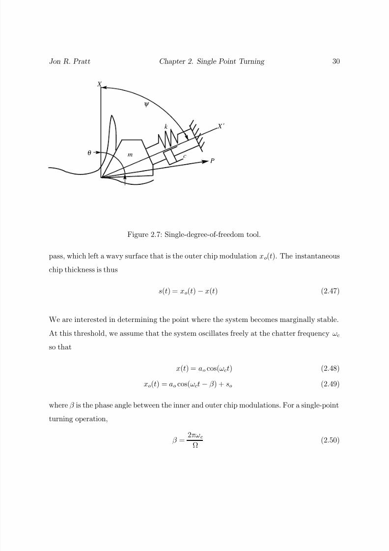
2.7 Single-degree-of-freedom tool. . . . . . . . . . . . . . . . . . . . . . . . . . 30
2.8 Stability lobes for the model of Hanna and Tobias (1974). . . . . . . . . . . 33
2.9 Two-degree-of-freedom cutting system. . . . . . . . . . . . . . . . . . . . . 34
2.10 Stability lobes for two-degree-of-freedom cutting system. . . . . . . . . . . 39
3.1 Vibration-absorber schemes: (a) semi-active and (b) fully active. Dashed
box represents a “virtual absorber”. . . . . . . . . . . . . . . . . . . . . . . 44
xiii

8/13/2019 Vibration Control for Chatter Suppression with Application to Boring Bars
http://slidepdf.com/reader/full/vibration-control-for-chatter-suppression-with-application-to-boring-bars 14/193
3.2 Linear stability diagram showing the critical width of cut as a function of the
rotational frequency. The upper curve corresponds to the controlled system
and the lower curve corresponds to the uncontrolled system. . . . . . . . . 50
4.1 Boring bar control system layout. . . . . . . . . . . . . . . . . . . . . . . . 55
4.2 Compensator electrical schematic. . . . . . . . . . . . . . . . . . . . . . . . 58
4.3 Bode plot of the tangential plant response function. The dashed line is the
experimentally measured response while the solid line is obtained from the
model. . . . . . . . . . . . . . . . . . . . . . . . . . . . . . . . . . . . . . . 59
4.4 Block diagram. . . . . . . . . . . . . . . . . . . . . . . . . . . . . . . . . . 60
4.5 Design results for various effective mass ratios. . . . . . . . . . . . . . . . . 66
4.6 Closed-loop performance; single-degree-of-freedom design (SDOF), matched
damping design (DAMP), and matched projections along the real axis (REAL). 67
4.7 Root locus of the system performance. . . . . . . . . . . . . . . . . . . . . 68
4.8 Bode plot of the predicted performance. . . . . . . . . . . . . . . . . . . . 69
4.9 Bode plot of the in situ tangential plant response function. . . . . . . . . . 69
5.1 Typical aluminum specimens,External File . . . . . . . . . . . . . . . . . . 72
5.2 A schematic of the test and measurement setup. . . . . . . . . . . . . . . . 73
5.3 Bifurcation diagram showing the amplitude of the fundamental harmonic of
chatter for various spindle speeds when w = 0.03 and feedrate = 0.0024 ipr. 74
xiv
8/13/2019 Vibration Control for Chatter Suppression with Application to Boring Bars
http://slidepdf.com/reader/full/vibration-control-for-chatter-suppression-with-application-to-boring-bars 15/193
5.4 Evolution of chatter in the tool response normal to the machined surface
when w = 0.002, speed = 90 rpm, and feedrate = 0.0024 ipr. . . . . . . . 76
5.5 The time trace of the steady-state chatter normal to the machined surface
when w = 0.002, speed = 90 rpm, and feedrate = 0.0024 ipr. . . . . . . . 76
5.6 The transient tool response to a hammer blow when w = 0.03, speed = 170
rpm, and feedrate = 0.0024 ipr. . . . . . . . . . . . . . . . . . . . . . . . . 77
5.7 Stable tool response normal (bottom trace) and tangential (top trace) to themachined surface when w = 0.03, speed = 190 rpm, and feedrate = 0.0024
ipr. Units are g’s. . . . . . . . . . . . . . . . . . . . . . . . . . . . . . . . . 79
5.8 Chattering tool response normal (bottom trace) and tangential (top trace)
to the machined surface when w = 0.03, speed = 190 rpm, and feedrate
= 0.0024 ipr. Units are g’s. . . . . . . . . . . . . . . . . . . . . . . . . . . . 79
5.9 Tangentially oriented chatter signature when w = 0.1
, speed = 235 rpm,and feedrate = 0.0024 ipr. . . . . . . . . . . . . . . . . . . . . . . . . . . . 80
5.10 Normally oriented chatter signature when w = 0.1, speed = 235 rpm, and
feedrate = 0.0024 ipr. . . . . . . . . . . . . . . . . . . . . . . . . . . . . . . 81
5.11 Chatter signature normal (bottom trace) and tangential (top trace) to the
machined surface when w = 0.005, speed = 195 rpm, and feedrate = 0.0024
ipr. Units are g’s. . . . . . . . . . . . . . . . . . . . . . . . . . . . . . . . . 81
5.12 Time traces, autospectra, cross-spectrum, and coherence when w = 0.002,
speed = 90 rpm, and feedrate = 0.0024 ipr. . . . . . . . . . . . . . . . . . . 82
xv
8/13/2019 Vibration Control for Chatter Suppression with Application to Boring Bars
http://slidepdf.com/reader/full/vibration-control-for-chatter-suppression-with-application-to-boring-bars 16/193
5.13 Time traces, autospectra, cross-spectra, and coherence when w = 0.03,
speed = 210 rpm, and feedrate 0.0024 ipr. . . . . . . . . . . . . . . . . . . 83
5.14 Time traces of the tool accelerations normal to the machined surface; ini-
tially, only tangential control is active; then, in addition, control is applied
in the normal direction to quench the chatter and eliminate the jump-type
instability; w = 0.002, speed = 170 rpm, and feedrate = 0.0024 ipr. . . . . 84
5.15 Time traces, autospectra, cross-spectrum, and coherence when w = 0.002,
speed = 180 rpm, feedrate = 0.0024 ipr, and tangential control is active . . 85
5.16 Time traces of the normal and tangential tool accelerations when w = 0.03,
speed = 230 rpm, and feedrate = 0.0024 ipr, before and after application of
biaxial control. . . . . . . . . . . . . . . . . . . . . . . . . . . . . . . . . . 86
5.17 An example of surface finish before and after application of the biaxial Smart
Tool control. External Figure . . . . . . . . . . . . . . . . . . . . . . . . . 86
5.18 Waterfall plot of autospectra obtained from ten consecutive ensembles. . . 87
6.1 Comparison of the phase portraits obtained using the method of harmonic
balance (a,c) with those obtained using numerical integration (b,d) when
τ = 1/75 for (a,b) w = 0.06 and (c,d) w = 0.136. . . . . . . . . . . . . . . . 95
xvi
8/13/2019 Vibration Control for Chatter Suppression with Application to Boring Bars
http://slidepdf.com/reader/full/vibration-control-for-chatter-suppression-with-application-to-boring-bars 17/193
6.2 Comparison of the nonlinear response curves obtained using the method of
harmonic balance for the case when τ = 1/75: thin lines obtained with a
six-term approximation and thick lines obtained with a two-term approxi-
mation. Both show supercritical Hopf bifurcations. Solid lines denote stable
trivial or periodic solutions, dotted lines denote unstable trivial or periodic
solutions, and dotted-dashed lines denote the region of quasiperiodic and
chaotic solutions. a is the amplitude of the fundamental harmonic of vibra-
tion and w is the width of cut. . . . . . . . . . . . . . . . . . . . . . . . . . 98
6.3 Comparison of the nonlinear response curves obtained using the method of
harmonic balance for the case when τ = 1/60: thin lines obtained with a six-
term approximation and thick lines obtained with a two-term approximation.
The two-term approximation erroneously predicts a subcritical rather than
a supercritical Hopf bifurcation. Solid lines denote stable trivial or periodic
solutions and dotted lines denote unstable trivial or periodic solutions. a is
the amplitude of the fundamental harmonic of vibration and w is the width
of cut. . . . . . . . . . . . . . . . . . . . . . . . . . . . . . . . . . . . . . . 99
6.4 Nonlinear response curves for a six-term approximation when w = 0.1. Solid
lines denote stable trivial or periodic solutions and dotted lines denote un-
stable trivial or periodic solutions. a is the amplitude of the fundamental
harmonic of vibration and w is the width of cut. . . . . . . . . . . . . . . . 100
6.5 The phase portrait (a) the Poincare section (b) the time history (c) and the
FFT (d) of the attractor obtained when τ = 1/75 and w = 0.136. . . . . . 104
6.6 The phase portrait (a) the Poincare section (b) the time history (c) and the
FFT (d) of the attractor obtained when τ = 1/75 and w = 0.141. . . . . . 105
xvii
8/13/2019 Vibration Control for Chatter Suppression with Application to Boring Bars
http://slidepdf.com/reader/full/vibration-control-for-chatter-suppression-with-application-to-boring-bars 18/193
6.7 The phase portrait (a) the Poincare section (b) the time history (c) and the
FFT (d) of the attractor obtained when τ = 1/75 and w = 0.230. . . . . . 105
6.8 The phase portrait (a) the Poincare section (b) the time history (c) and the
FFT (d) of the attractor obtained when τ = 1/75 and w = 0.240. . . . . . 106
6.9 The Poincare sections obtained when τ = 1/75 and w = (a) 0.250 (b) 0.255
(c) 0.260 (d) 0.265 (e) 0.266 and (f) 0.267. . . . . . . . . . . . . . . . . . . 107
6.10 The Poincare sections obtained when τ = 1/75 and w = (a) 0.270 (b) 0.30(c) 0.32 and (d) 0.35. . . . . . . . . . . . . . . . . . . . . . . . . . . . . . . 107
6.11 Comparison of the nonlinear response curves obtained with a six-term ap-
proximation with nonlinear stiffness (thin lines) and linear stiffness (thin
lines) when (a) τ = 1/60 and (b) τ = 1/75. Solid lines denote stable trivial
or periodic solutions and dotted-dashed lines denote unstable trivial or peri-
odic solutions. a is the amplitude of the fundamental harmonic of vibration
and w is the width of cut. . . . . . . . . . . . . . . . . . . . . . . . . . . . 108
6.12 Comparison of nonlinear response curves obtained from analog simulation
with the results obtained from a six-term harmonic balance solution when (a)
τ = 1/75 and (b) τ = 1/60. Solid lines denote stable periodic solutions and
dotted lines denote unstable periodic solutions determined in the previous
analysis. Diamonds denote points obtained via analog computer. . . . . . . 116
6.13 Power spectrum of the response for τ = 1/60 and w = 0.200. . . . . . . . . 117
6.14 The phase portraits (a) and (e), the Poincare sections (b) and (f), the time
histories (c) and (g), and the power spectra (d) and (h) of the attractors
obtained when τ = 1/75 and w = 0.060 and w = 0.136, respectively. . . . . 118
xviii
8/13/2019 Vibration Control for Chatter Suppression with Application to Boring Bars
http://slidepdf.com/reader/full/vibration-control-for-chatter-suppression-with-application-to-boring-bars 19/193
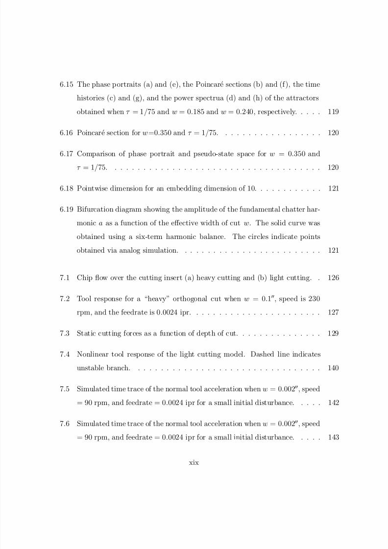
6.15 The phase portraits (a) and (e), the Poincare sections (b) and (f), the time
histories (c) and (g), and the power spectrua (d) and (h) of the attractors
obtained when τ = 1/75 and w = 0.185 and w = 0.240, respectively. . . . . 119
6.16 Poincare section for w=0.350 and τ = 1/75. . . . . . . . . . . . . . . . . . 120
6.17 Comparison of phase portrait and pseudo-state space for w = 0.350 and
τ = 1/75. . . . . . . . . . . . . . . . . . . . . . . . . . . . . . . . . . . . . 120
6.18 Pointwise dimension for an embedding dimension of 10. . . . . . . . . . . . 121
6.19 Bifurcation diagram showing the amplitude of the fundamental chatter har-
monic a as a function of the effective width of cut w. The solid curve was
obtained using a six-term harmonic balance. The circles indicate points
obtained via analog simulation. . . . . . . . . . . . . . . . . . . . . . . . . 121
7.1 Chip flow over the cutting insert (a) heavy cutting and (b) light cutting. . 126
7.2 Tool response for a “heavy” orthogonal cut when w = 0.1, speed is 230
rpm, and the feedrate is 0.0024 ipr. . . . . . . . . . . . . . . . . . . . . . . 127
7.3 Static cutting forces as a function of depth of cut. . . . . . . . . . . . . . . 129
7.4 Nonlinear tool response of the light cutting model. Dashed line indicates
unstable branch. . . . . . . . . . . . . . . . . . . . . . . . . . . . . . . . . 140
7.5 Simulated time trace of the normal tool acceleration when w = 0.002, speed
= 90 rpm, and feedrate = 0.0024 ipr for a small initial disturbance. . . . . 142
7.6 Simulated time trace of the normal tool acceleration when w = 0.002, speed
= 90 rpm, and feedrate = 0.0024 ipr for a small initial disturbance. . . . . 143
xix
8/13/2019 Vibration Control for Chatter Suppression with Application to Boring Bars
http://slidepdf.com/reader/full/vibration-control-for-chatter-suppression-with-application-to-boring-bars 20/193
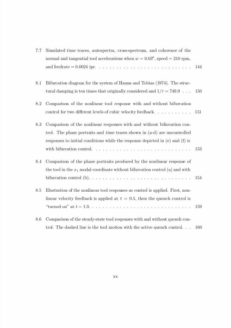
7.7 Simulated time traces, autospectra, cross-spectrum, and coherence of the
normal and tangential tool accelerations when w = 0.03, speed = 210 rpm,
and feedrate = 0.0024 ipr. . . . . . . . . . . . . . . . . . . . . . . . . . . . 144
8.1 Bifurcation diagram for the system of Hanna and Tobias (1974). The struc-
tural damping is ten times that originally considered and 1/τ = 749.9 . . . 150
8.2 Comparison of the nonlinear tool response with and without bifurcation
control for two different levels of cubic velocity feedback. . . . . . . . . . . 151
8.3 Comparison of the nonlinear responses with and without bifurcation con-
trol. The phase portraits and time traces shown in (a-d) are uncontrolled
responses to initial conditions while the response depicted in (e) and (f) is
with bifurcation control. . . . . . . . . . . . . . . . . . . . . . . . . . . . . 153
8.4 Comparison of the phase portraits produced by the nonlinear response of
the tool in the x1 modal coordinate without bifurcation control (a) and with
bifurcation control (b). . . . . . . . . . . . . . . . . . . . . . . . . . . . . . 154
8.5 Illustration of the nonlinear tool responses as control is applied. First, non-
linear velocity feedback is applied at t = 0.5, then the quench control is
“turned on” at t = 1.0. . . . . . . . . . . . . . . . . . . . . . . . . . . . . . 159
8.6 Comparison of the steady-state tool responses with and without quench con-
trol. The dashed line is the tool motion with the active quench control. . . 160
xx

8/13/2019 Vibration Control for Chatter Suppression with Application to Boring Bars
http://slidepdf.com/reader/full/vibration-control-for-chatter-suppression-with-application-to-boring-bars 21/193
List of Tables
4.1 Estimated dynamic properties of the tangential control system. . . . . . . . 61
xxi
8/13/2019 Vibration Control for Chatter Suppression with Application to Boring Bars
http://slidepdf.com/reader/full/vibration-control-for-chatter-suppression-with-application-to-boring-bars 22/193
Chapter 1
Introduction
1.1 Background and Motivation
Extensive research has been devoted to the characterization, modelling, and control of vi-
brations that occur when machine tools operate at the limit of their dynamic stability.
These vibrations, known as machine-tool chatter, must be avoided to maintain machining
tolerances, preserve surface finish, and prevent tool breakage. To avoid chatter, machine-
tool users limit material removal rates in order to stay within the dynamic stability bound-
ary of their machines. ¿From a manufacturing stand point, chatter is a constraint on the
machine-tool user that limits the available production capacity. Thus, vibration-control
methods for extending machine-tool operating envelopes are highly desirable.
1
8/13/2019 Vibration Control for Chatter Suppression with Application to Boring Bars
http://slidepdf.com/reader/full/vibration-control-for-chatter-suppression-with-application-to-boring-bars 23/193
Jon R. Pratt Chapter 1. Introduction 2
1.1.1 Chatter Mechanisms
Machine-tool chatter is thought to occur for a variety of reasons. The excellent monographs
by Tobias (1965) and Koeingsburger and Tlusty (1970) document much of the pioneering
work in the field. These authors were the first to identify the mechanisms known as
regeneration (Tobias and Fishwick, 1958) and mode coupling (Koeingsburger and Tlusty,
1970).
Briefly, regenerative chatter occurs whenever cuts overlap and the cut produced at time
t leaves small waves in the material that are regenerated with each subsequent pass of
the tool. It is considered to be the dominant mechanism of chatter in turning operations.
If regenerative tool vibrations become large enough that the tool looses contact with the
workpiece, then a type of chatter known as multiple regenerative chatter occurs. This
mechanism has been the subject of studies by Shi and Tobias (1984), Kondo, Kawano, and
Sato (1981), and Tlusty and Ismail (1982).
Mode coupling occurs whenever the relative vibration between the tool and the workpiece
exists simultaneously in at least two directions in the plane of the cut. In this case, the
tool traces out an elliptic path that varies the depth of cut in such a fashion as to feed
the coupled modes of vibration. It is considered to be a factor when chatter develops in
slender nearly symmetric tools, such as boring bars. We note the similarity between this
mechanism and the phenomenon of aeroelastic flutter.
Other mechanisms have been postulated. Arnold (1946) suggested that the cutting forces
depend on the velocity in such a fashion as to produce negative damping. This chatter
mechanism is essentially a frictional effect and has characteristics similar to that of the
well-known Rayleigh oscillator (Nayfeh and Mook, 1979).
The foregoing are all mechanisms that lead to self-excited oscillations. Forced vibrations
8/13/2019 Vibration Control for Chatter Suppression with Application to Boring Bars
http://slidepdf.com/reader/full/vibration-control-for-chatter-suppression-with-application-to-boring-bars 24/193
Jon R. Pratt Chapter 1. Introduction 3
also occur. A common source of such vibrations in turning operations is rotating imbal-
ance or misalignment of the workpiece. Tool runout and spindle errors also cause forced
vibrations. Milling operations generally produce interrupted cuts as the cutters rotate in
and out of the workpiece. These so-called interrupted cuts lead to impact oscillations, a
form of forced machine-tool vibration that has been studied by Davies and Balachandran
(1996).
1.1.2 Existing Chatter Mitigation Strategies
It is generally accepted that stiff highly damped tools have a lower tendency to chatter.
Rivin and Kang (1989) substantially increased the damping of a lathe tool by using a
sandwich of steel plates and hard rubber viscoelastic material to form a laminated clamping
device to hold the tool. Kelson and Hsueh (1996) also achieved an increase in stability by
redesigning the tool holder for added stiffness and damping. A patent for a damping
sandwich of plural layers of steel and plural alternate layers of viscoelastic solid material
was awarded to Seifring (1991) and assigned to the Monarch Machine Tool Company.
Tobias (1965) cites a number of instances where passive vibration absorbers of various
configurations have been applied with success. He describes applications using a Lanchester
absorber, a dynamic vibration absorber, and an impact absorber. Boring bars with passive
vibration absorbers incorporated into the tool shank have been available from Kennametal
for some time (see, for instance, Kosker, 1975), and a patent for a similar device was
awarded to Hopkins (1974) and assigned to the Valeron Corporation.
Researchers have also found that the cutting speed can be modulated to enhance stability
(Sexton, Milne, and Stone, 1977; Takemura, etal 1974). Parametric variation of the tool
stiffness has also been proposed as a method for suppressing regenerative chatter (Segalman
8/13/2019 Vibration Control for Chatter Suppression with Application to Boring Bars
http://slidepdf.com/reader/full/vibration-control-for-chatter-suppression-with-application-to-boring-bars 25/193
Jon R. Pratt Chapter 1. Introduction 4
and Redmond, 1996).
A variety of patents exist for devices that detect chatter and then adjust the process
parameters, such as speed and feed, to produce a stable cut. A patent for a system that
detects the “lobe precession” angle during single-point turning and adjusts the cross feed to
maintain stability was awarded to Thompson (1986) and assigned to the General Electric
Company. A fundamental assumption of this type of chatter mitigation technique is that
a supercritical bifurcation exists, or in other words, the transition from static to dynamic
cutting is smooth and free of jump phenomena. Drawing an analogy to aerodynamic flutter,
one assumes that by simply decreasing the aircraft/workpiece velocity the flutter/chatter
will go away.
More aggressive active control solutions have been sought. Nachtigal, Klein, and Maddux
(1976) patented an “apparatus for controlling vibrational chatter in a machine-tool utilizing
an updated synthesis circuit”. By sensing tool motion, the authors claimed they could
model the cutting forces in their circuit and apply appropriate counteracting forces via an
actuator. Recently, Tewani, Rouch, and Walcott (1995) demonstrated chatter control of a
boring bar by using what they call an active dynamic absorber. They also patented the
device (Rouch etal, 1991).
The active control scheme of Tewani, Rouch, and Walcott (1995) is the nearest in spirit
to the control scheme demonstrated in this Dissertation and, so, deserves a closer scrutiny.
The device which they patented uses a piezoelectric reaction-mass actuator mounted inside
the boring bar. The reaction-mass actuator is modelled as an additional degree of freedom
coupled to the boring bar through a spring, dashpot, and control force. The bar itself
is modelled using a single-degree-of-freedom lumped-parameter approximation of the first
mode of a cantilever beam. Accelerations of the boring bar and reaction mass are sensed
and conditioned to yield signals proportional to the four state variables of the system.
8/13/2019 Vibration Control for Chatter Suppression with Application to Boring Bars
http://slidepdf.com/reader/full/vibration-control-for-chatter-suppression-with-application-to-boring-bars 26/193
Jon R. Pratt Chapter 1. Introduction 5
The combination of bar and actuator has the classic configuration of the two-degree-of-
freedom dynamic vibration absorber analyzed by Den Hartog (1985), but with the added
functionality of the active dynamic absorber analysed by Tewani, Walcott, and Rouch
(1991). The authors use optimal control techniques to obtain state-variable feedback gains.
The resulting system has a highly-damped driving-point frequency-response function that
produces a substantial increase in the predicted stable width of cut. Cutting tests using
this system reveal stability problems for length-to-diameter ratios of 9 or more (Tewani,
Switzer, Walcott, Rouch, and Massa, 1993). The authors state that, because of nonlinear
actuator dynamics, the control was at times incapable of maintaining a stable cut.
The instability described by Tewani et al. (1993) seems to be similar to the subcritical
cutting stability reported by Hooke and Tobias (1964) for turning operations on a lathe and
by Hanna and Tobias (1974) for face milling operations on a vertical mill. To address this
stabiltiy, Hanna and Tobias (1974) developed a nonlinear single-degree-of-freedom model
based on experimental identification of the structure and cutting force. This model was
studied recently by Nayfeh, Chin, and Pratt (1997) who found an analytical expression
for the normal form of the bifurcation, used harmonic balance to reveal the true nature of
the subcritical stability, and discovered that the model posesses a torus-doubling route to
chaos. Pratt and Nayfeh (1996) confirmed this analysis using analog computer simulations.
All previous attempts at chatter control in boring bars have assumed that chatter may be
characterized by a single mode of vibration. We will show in this Dissertation, through
experiment, simulation, and theory, that multiple modes of chatter vibration can coexist,
and that to insure a robust and effective control system it is necessary to apply control
forces in two-orthogonal directions.
8/13/2019 Vibration Control for Chatter Suppression with Application to Boring Bars
http://slidepdf.com/reader/full/vibration-control-for-chatter-suppression-with-application-to-boring-bars 27/193
Jon R. Pratt Chapter 1. Introduction 6
1.2 Organization of the Dissertation
The Dissertation is divided into two parts. In Part I, we treat the linear chatter control
problem, whereas in Part II we consider complications that arise due to nonlinearity.
We begin Chapter 2 with a brief overview of the machine-tool structure and cutting process,
reviewing the nomenclature and geometry of single-point turning. Working from these
definitions, we review the standard approaches to static cutting-force modeling and some
of the ways these techniques are extended to the dynamic condition. Next, we take up thelinear regenerative chatter theory, which is essentially the problem of time-delay feedback.
We make the important observation that the regenerative cutting force acts like a negative
damping. The linear stability is developed as a function of depth of cut and workpiece
rotational speed. We find that the machine-tool structure becomes marginally stable when
the negative damping of the cutting force balances the positive damping inherent in the
flexible tool. The point at which stability is lost is a Hopf bifurcation point for the nonlinear
system, a topic that is taken up in Part II of the Dissertation.
In Chapter 3, we seek an active control solution to increase the overall system damping and
thereby extend the operating envelope of the boring bar. We consider various vibration con-
trol options and select an active strategy that uses 2nd-order feedback compensation. We
demonstrate through an example from the literature how the addition of the compensator
can greatly extend the limit width of cut.
Part I of the Dissertation comes to a close in Chapter 4. In this chapter, a prototype
chatter control system is presented. Actuators and sensors are selected and the issues
surrounding their placement are discussed. A block diagram of the control system is de-
veloped. Modal parameters are determined for the combined boring-bar-actuator system.
The frequency-response characteristics are determined experimentally and a mathematical

8/13/2019 Vibration Control for Chatter Suppression with Application to Boring Bars
http://slidepdf.com/reader/full/vibration-control-for-chatter-suppression-with-application-to-boring-bars 28/193

8/13/2019 Vibration Control for Chatter Suppression with Application to Boring Bars
http://slidepdf.com/reader/full/vibration-control-for-chatter-suppression-with-application-to-boring-bars 29/193
Jon R. Pratt Chapter 1. Introduction 8
We close the Dissertation by summarizing our findings and making recommendations for
future research.
8/13/2019 Vibration Control for Chatter Suppression with Application to Boring Bars
http://slidepdf.com/reader/full/vibration-control-for-chatter-suppression-with-application-to-boring-bars 30/193
Part I
Linear Machine-Tool Dynamics and
Control
9

8/13/2019 Vibration Control for Chatter Suppression with Application to Boring Bars
http://slidepdf.com/reader/full/vibration-control-for-chatter-suppression-with-application-to-boring-bars 31/193
Chapter 2
The Statics and Dynamics of
Single-Point Turning
The conversion of raw material into manufactured products usually requires that some
sort of material removal process be performed. By far the most common material removalprocesses are the so-called chip-forming types. Chip forming, or the act of shaving metal
from a workpiece to produce a desired geometric shape, is carried out using a machine tool.
The type of machine tool used to manufacture a product, its general shape and orientation
of cutting surfaces, is dictated to a large extent by the eventual geometry and surface finish
desired for the end product.
Milling machines, engine lathes, twist drills, and shaping and planing machines are but a
few examples of the diverse types of machine tools that exist. One way in which machine
tools are distinguished from one another is by the number of cutting surfaces, or cutters,
employed to remove the metal. In this respect, machine tools are referred to as either
single-point, or multipoint, according to the common convention.
10

8/13/2019 Vibration Control for Chatter Suppression with Application to Boring Bars
http://slidepdf.com/reader/full/vibration-control-for-chatter-suppression-with-application-to-boring-bars 32/193
Jon R. Pratt Chapter 2. Single Point Turning 11
We will be concerned with single-point tools. Specifically, we will consider a boring oper-
ation on an engine lathe. Boring bars, as will be seen, are particularly prone to dynamic
instability due to their relatively high flexibility and low damping. This particular tool
and manufacturing process are amenable for study because the structural dynamics are
reasonably well characterized using a low-order model.
In the remainder of this chapter we summarize the background material necessary to an
understanding of the problem. This is a mature subject area, and a number of fine text
books are available that treat the material in greater detail (Tobias, 1965; King, 1985;
Armarego and Brown, 1969; Boothroyd, 1975). The following is intended as an introduction
to the terminology and physics of the problem for the reader who may be new to the subject.
2.1 Boring Bars and Engine Lathes
An engine lathe is illustrated in Fig. 2.1. The machine consists of a headstock (A) mounted
on the lathe bed (B). The headstock contains the spindle (C) that rotates the cylinderical
workpiece (D) that is gripped in the chuck (E). The single-point cutting tool (F), in this
case a boring bar, is held in the toolholder (G) mounted on the cross slide (H). The cross
slide is in turn mounted to the carriage (I).
Boring produces an internal cylinderical surface. Generally, one begins with a cylinderical
workpiece of some nominal inner diameter that must be bored out to a larger diameter of
specified tolerance.
The machining parameters controlled by an operator are the cutting speed V , the feedrate
r, and the depth of cut w that are illustrated in Fig 2.2 for a single-point turning operation.
The cutting speed refers to the relative velocity between the tool and the workpiece. It is

8/13/2019 Vibration Control for Chatter Suppression with Application to Boring Bars
http://slidepdf.com/reader/full/vibration-control-for-chatter-suppression-with-application-to-boring-bars 33/193
Jon R. Pratt Chapter 2. Single Point Turning 12
+y
+x
+z
A
B
C
D
E
F G
H
I
J
Figure 2.1: Engine lathe.
a function of the spindle revolutions per minute and workpiece diameter and has units of
velocity (f.p.m. or m s−1). The speed is sometimes referred to as the primary motion and
is measured along the y direction. The feedrate is a measure of the carriage motion. It is
expressed in terms of the distance the carriage moves towards the headstock (the “feed”
so) per spindle revolution (i.p.r. or mm rev−1) and is measured along the z direction. The
carriage and spindle are connected by gearing and a lead screw (item (J) of Fig. 2.1) so
that the two motions are synchronized. Thus, as the workpiece rotates, the machine feeds
the tool in the z direction. Finally, the depth of cut is a measure of the amount of material
to be removed, has units of length (in or mm), and is measured along the x direction.
As the chip forms, it produces the transient and machined surfaces of Fig. 2.2 (a). We see
that the machined surface is of a diameter that is decreased by twice the depth of cut for

8/13/2019 Vibration Control for Chatter Suppression with Application to Boring Bars
http://slidepdf.com/reader/full/vibration-control-for-chatter-suppression-with-application-to-boring-bars 34/193
Jon R. Pratt Chapter 2. Single Point Turning 13
single-point turning (analogously, the diameter is increased by twice the depth of cut for
single-point boring). Section AA of Fig. 2.2 shows the chip flowing over the tool in the
y − z plane, sometimes referred to as the working plane.
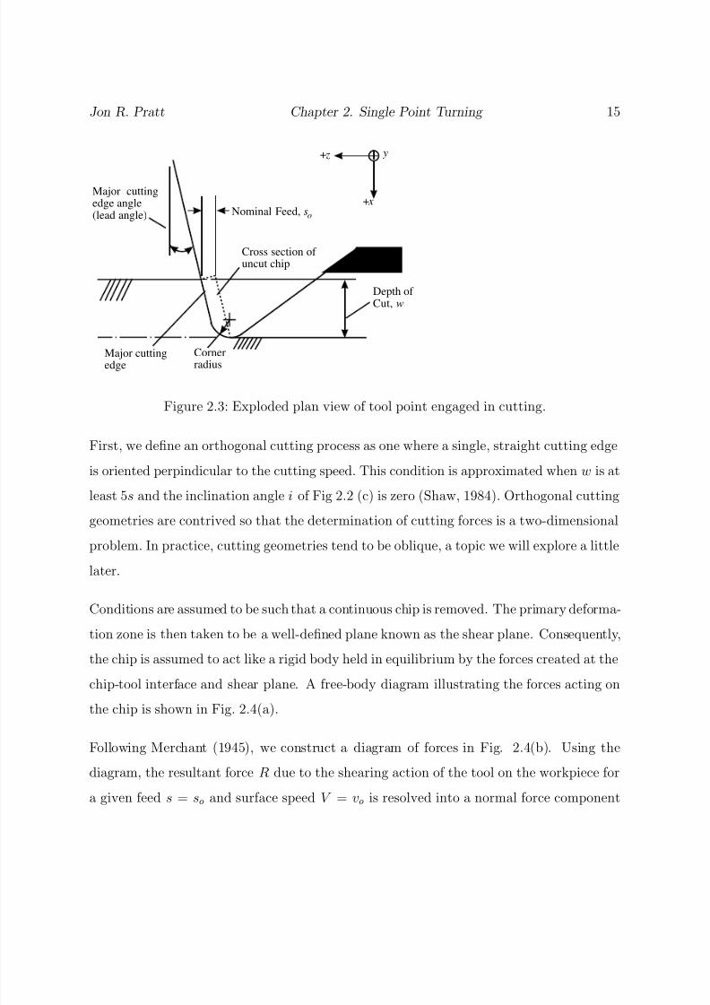
In Fig. 2.3, we see an exploded plan view of the tool point while it is engaged in cutting.
The cross section of the uncut chip is seen to depend on the feed, the lead angle, and the
corner radius. For steady cutting, the undeformed chip thickness s is simply the feed so.
The area of the uncut chip influences the power required to carry out the operation and is
often used to characterize the cutting forces.
2.2 Mechanics of Metal Removal
The forces that arise during metal removal are classified as either static or dynamic. There
is a well established literature concerning the modelling and analysis of both classes. In
this section we begin with the classic shear plane models for static orthogonal cutting and
then review how researchers have tried to develop dynamic cutting force models.
2.2.1 Static Orthogonal Cutting with a Single Edge
A thin-shear-plane model is often used as the basis for the characterization of static cutting
forces. This type of solution is referred to as a shear-angle solution, or Merchant analysis
when crediting its originator (Merchant, 1945). The theory of Merchant is popular becauseit purportedly results in an upper bound solution for the cutting forces. Thus, it is conser-
vative and provides a simple way to deal qualitatively with what is at present a difficult if
not intractable problem.

8/13/2019 Vibration Control for Chatter Suppression with Application to Boring Bars
http://slidepdf.com/reader/full/vibration-control-for-chatter-suppression-with-application-to-boring-bars 35/193
Jon R. Pratt Chapter 2. Single Point Turning 14
Workpiece
Transient surface
Machined surface
V
r
Ω
w
(a)
w
s
V
A A
i
(c)(b)
V
s
α
(d)
Section AA (i =0)
Figure 2.2: Single-point turning. (a) Oblique view, (b) plan view, (c) side view, and (d)
section AA.
8/13/2019 Vibration Control for Chatter Suppression with Application to Boring Bars
http://slidepdf.com/reader/full/vibration-control-for-chatter-suppression-with-application-to-boring-bars 36/193
Jon R. Pratt Chapter 2. Single Point Turning 15
Major cuttingedge angle(lead angle) Nominal Feed, s
Depth ofCut, w
Major cuttingedge
Cornerradius
Cross section ofuncut chip
+x
+z y
o
Figure 2.3: Exploded plan view of tool point engaged in cutting.
First, we define an orthogonal cutting process as one where a single, straight cutting edge
is oriented perpindicular to the cutting speed. This condition is approximated when w is at
least 5s and the inclination angle i of Fig 2.2 (c) is zero (Shaw, 1984). Orthogonal cutting
geometries are contrived so that the determination of cutting forces is a two-dimensionalproblem. In practice, cutting geometries tend to be oblique, a topic we will explore a little
later.
Conditions are assumed to be such that a continuous chip is removed. The primary deforma-
tion zone is then taken to be a well-defined plane known as the shear plane. Consequently,
the chip is assumed to act like a rigid body held in equilibrium by the forces created at the
chip-tool interface and shear plane. A free-body diagram illustrating the forces acting on
the chip is shown in Fig. 2.4(a).
Following Merchant (1945), we construct a diagram of forces in Fig. 2.4(b). Using the
diagram, the resultant force R due to the shearing action of the tool on the workpiece for
a given feed s = so and surface speed V = vo is resolved into a normal force component

8/13/2019 Vibration Control for Chatter Suppression with Application to Boring Bars
http://slidepdf.com/reader/full/vibration-control-for-chatter-suppression-with-application-to-boring-bars 37/193

8/13/2019 Vibration Control for Chatter Suppression with Application to Boring Bars
http://slidepdf.com/reader/full/vibration-control-for-chatter-suppression-with-application-to-boring-bars 38/193
Jon R. Pratt Chapter 2. Single Point Turning 17
From the continuity relation, the chip thickness ratio is defined as
ρ = so
sc
= vc
vo
(2.4)
and from the geometry of Fig. 2.4 (b)
tan φ = ρ cos α
1 − ρ sin α (2.5)
A number of thin-zone models have been proposed that are variants of the Merchant anal-
ysis (Stabler, 1951; Lee and Schaffer, 1951; Oxley, 1961; Kobayashi and Thomsen, 1962;Hastings, Mathew, and Oxley, 1980). Discussions of the assumptions and relative merits of
these and other models for static cutting can be found in Shaw (1984), Boothroyd (1975),
Armarego and Brown (1969), Kalpakjian (1992), and Oxley (1989). It is important to
note, as all the authors point out, that none of these models matches the experimental
data outside of the narrow range of values for which it has been adapted. However, it is
generally accepted that for a given set of cutting conditions, an empirical relation of the
form
φ = C 1 − C 2(β − α) (2.6)
can be found among the angles where C 1 and C 2 are constants. Thus, for steady-state
orthogonal cutting conditions, the cutting force is a constant and proportional to the area
of the uncut chip for a fixed speed.
2.2.2 Oblique Cutting
One seldom encounters a truely orthogonal cut in practice. Nearly all practical cutting
processes are oblique; that is, the tool’s cutting edge is inclined to the relative velocity
between the tool and the workpiece as shown in Fig. 2.5. Furthermore, most tools engage

8/13/2019 Vibration Control for Chatter Suppression with Application to Boring Bars
http://slidepdf.com/reader/full/vibration-control-for-chatter-suppression-with-application-to-boring-bars 39/193
Jon R. Pratt Chapter 2. Single Point Turning 18
w
i
w
v
vo
c
c
ηc
Chip
Figure 2.5: Plan view of oblique cutting geometry.
two or more cutting edges at a time, as occurs along the toolnose in the exploded view of
the tool point shown in Fig. 2.3.
The mechanics of oblique cutting may be determined using a thin-shear-plane model. De-
scriptions of this type of cutting theory are presented by Armarego and Brown (1969) and
Shaw (1984). The original work is most often credited to Stabler (1951). The problem is
worked out by finding the inclination angle for the given tool geometry and using this in-
formation, along with the chip flow direction, to construct an equivalent orthogonal cutting
condition. Techniques for working out the geometry and deriving the forces are explained
in Armarego and Brown (1969) and in Shaw (1984).

8/13/2019 Vibration Control for Chatter Suppression with Application to Boring Bars
http://slidepdf.com/reader/full/vibration-control-for-chatter-suppression-with-application-to-boring-bars 40/193
Jon R. Pratt Chapter 2. Single Point Turning 19
Armarego and Brown (1969) suggest the following relations for the the cutting and thrust
forces:
F c = swτ ssin φn
cos(β n − αn) + tan i tan ηc sin β n
cos2 (φn + β n − αn) + tan2 ηc sin2 β n
(2.7)
F t = swτ ssin φn
cos(β n − αn)tan i − tan ηc sin β n
cos2 (φn + β n − αn) + tan2 ηc sin2 β n
(2.8)
where φn, β n, and αn are the shear angle, friction angle, and rake angle in the plane normal
to the cutting edge. They are determined by consideration of the oblique geometry as
characterized by the angle of inclination i and the chip-flow direction ηc.
A theory for oblique cutting geometries that invlolves multiple edges is still being developed.
For instance, an upper bound cutting model for oblique cutting tools possessing a nose
radius, essentially the problem of Fig. 2.3, was recently proposed by Seethaler and Yellowley
(1997). It supposes the existence of multiple shear planes that may be treated as a series
of single-edge cutting problems subject to the constraint that the chip leave the tool as a
rigid body.
2.2.3 Summary of Static Cutting Force Models
A review of the literature reveals a dizzying array of static cutting-force models. Though
none of the models can be said to accurately predict cutting forces for the most general
cases, a consensus does seem to exist that a thin-shear-zone model, as proposed by Merchant
(1945), can provide an upper bound solution.
For the purposes of this Dissertation, the most important observation that can be made is
that the cutting forces are dependent on the undeformed chip area. This conclusion holds
for both orthogonal and oblique geometries. It appears that, for a single-edged cut of fixed
speed and width, the cutting forces will depend entirely on the undeformed chip thickness.

8/13/2019 Vibration Control for Chatter Suppression with Application to Boring Bars
http://slidepdf.com/reader/full/vibration-control-for-chatter-suppression-with-application-to-boring-bars 41/193
Jon R. Pratt Chapter 2. Single Point Turning 20
2.2.4 Dynamic Orthogonal Cutting
The problem of tool motion while machining with an orthogonal cutting geometry is illus-
trated in Fig. 2.6. The undeformed chip thickness is variable due to the outer and inner
chip modulations. Inner chip modulations are the result of tool motions x(t) and y(t) that
generate a wavy surface during the present tool pass. During the next tool pass, this wavy
surface is removed and becomes the outer surface of the chip. Hence, for the case of an
orthogonal turning operation with a single cutting edge, the outer chip modulations are
due to tool motions that ocurred during the previous tool pass and may be characterized
by the tool dispacements xo(t) = xτ + so and yo(t) = yτ , where xτ = x(t−τ ), yτ = y(t−τ ),
and τ is the period of one workpiece revolution.
Tool
x x
y y
Y
X
o
oα
φ
Figure 2.6: Dynamic orthogonal cutting.
The production of an inner chip modulation by the tool is commonly referred to as wave
generation. In a similar fashion, the removal of the outer chip modulation is often referred
to as wave removal. Clearly, the chip thickness varies due to wave generation and removal.
Furthermore, it seems that the shear angle should vary as well.

8/13/2019 Vibration Control for Chatter Suppression with Application to Boring Bars
http://slidepdf.com/reader/full/vibration-control-for-chatter-suppression-with-application-to-boring-bars 42/193
Jon R. Pratt Chapter 2. Single Point Turning 21
Numerous approaches have been devised to account for the forces generated as a result of
wave generation and removal. Some investigators work from Merchant’s model and seek
an explicit expression for the fluctuation of the shear angle in order to obtain the dynamic
forces. Other researchers take a more empirical approach. Space considerations preclude a
detailed discussion of all of these approaches, but some represenative treatments follow.
The model of Tobias and Fishwick (1958)
Tobias and Fishwick hypothesised that, under dynamic cutting conditions, the cutting force
P is a function of three independent factors, or P (s,r, Ω) where s is the undeformed chip
thickness, r is the feedrate, and Ω is the spindle rotational speed. Hence, the cutting-force
variation for small changes in these factors is
dP = k1ds + k2dr + k3dΩ (2.9)
where k1, k2, and k3 are dynamic cutting coefficients such that
k1 =
∂P
∂s
dr=dΩ=0
, k2 =
∂P
∂r
ds=dΩ=0
, k3 =
∂P
∂ Ω
dr=ds=0
Tobias (1965) related the dynamic cutting coefficients to the static force coefficients to
obtain
dP = k1ds + 2πK
Ω dr +
kΩ −
2πK
Ω s0
dΩ (2.10)
where k1 is a dynamic coefficient termed the chip thickness ratio, K = ks − k1 is the
penetration coefficient , ks and kΩ are static force coefficients relative to the undeformed
chip thickness and speed, respectively, and s0 is the steady-state undeformed chip thickness.The values for these coefficients are determined at a nominal speed vo and feedrate ro. The
force dP depends linearly on the width of cut w, and it has become customary to factor
out this dependence and write
dP = w
k1ds + 2πK
Ω dr +
kΩ −
2πK
Ω s0
dΩ
(2.11)
8/13/2019 Vibration Control for Chatter Suppression with Application to Boring Bars
http://slidepdf.com/reader/full/vibration-control-for-chatter-suppression-with-application-to-boring-bars 43/193
Jon R. Pratt Chapter 2. Single Point Turning 22
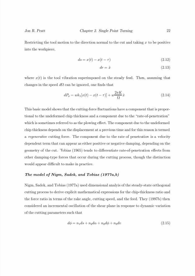
Restricting the tool motion to the direction normal to the cut and taking x to be positive
into the workpiece,
ds = x(t) − x(t − τ ) (2.12)
dr = x (2.13)
where x(t) is the tool vibration superimposed on the steady feed. Then, assuming that
changes in the speed dΩ can be ignored, one finds that
dP x = wk1[x(t)− x(t− τ )] + w
2πK
Ω x (2.14)
This basic model shows that the cutting-force fluctuations have a component that is propor-
tional to the undeformed chip thickness and a component due to the “rate-of-penetration”
which is sometimes referred to as the plowing effect. The component due to the undeformed
chip thickness depends on the displacement at a previous time and for this reason is termed
a regenerative cutting force. The component due to the rate of penetration is a velocity
dependent term that can appear as either positive or negative damping, depending on thegeometry of the cut. Tobias (1965) tends to differentiate rate-of-penetration effects from
other damping-type forces that occur during the cutting process, though the distinction
would appear difficult to make in practice.
The model of Nigm, Sadek, and Tobias (1977a,b)
Nigm, Sadek, and Tobias (1977a) used dimensional analyis of the steady-state orthogonal
cutting process to derive explicit mathematical expressions for the chip-thickness ratio andthe force ratio in terms of the rake angle, cutting speed, and the feed. They (1997b) then
considered an incremental oscillation of the shear plane in response to dynamic variation
of the cutting parameters such that
dφ = n1ds + n2dα + n2dφ + n3dv (2.15)

8/13/2019 Vibration Control for Chatter Suppression with Application to Boring Bars
http://slidepdf.com/reader/full/vibration-control-for-chatter-suppression-with-application-to-boring-bars 44/193
Jon R. Pratt Chapter 2. Single Point Turning 23
They found the following expressions for the incremental force components:
dP x = wk1c
C 1(x − xτ ) + C 2
xv0
+ C 3
xv0− xτ
v0
(2.16)
dP y = wk1c
T 1(x − xτ ) + T 2
x
v0+ T 3
x
v0−
xτ
v0
(2.17)
where the x direction is taken to be positive into the material, x and xτ are the deviations
of the tool from its prescribed path during the present and former tool passes, respectively,
and C 1, C 2, C 3, T 1, T 2, and T 3 are cutting coefficients determined by the geometry of the
cut.
The model of Wu and Liu (1985a,b)
Wu and Liu (1985a) begin with the Merchant Eqs. (2.1) and (2.2) and assume that an
exponential form for the mean friction coefficient µ = tan β can be obtained from static
cutting measurements. They use an approximate form of the continuity relationship of Eq.
(2.5) in conjunction with the shear-angle formula
φ = 1
2
C m −1
2
(β − α) (2.18)
to derive the following dynamic shear-angle relation:
cot φ = (Aφ − Cφv0) + Bφ
2 (x− xo) −
C φ2
(y − yo) (2.19)
where Aφ, Bφ, and C φ are the dynamic shear-angle coefficients evaluated at a given cutting
condition with mean shear angle φ0 and cutting speed v0, see Wu and Liu (1985a) for the
explicit expressions. The relationship represents a first-degree approximation for shear-
angle oscillations about the mean cutting condition when the tool is free to oscillate both
normal and tangential to the machined surface.
Wu and Liu substitute the dynamic shear-angle relation into Eqs. (2.1) and (2.2) and
obtain
P x = −2wτ (xo − x)[(Ax − C xv0) + 1
2Bx(x − xo) −
1
2C x(y − yo)] + f p (2.20)
8/13/2019 Vibration Control for Chatter Suppression with Application to Boring Bars
http://slidepdf.com/reader/full/vibration-control-for-chatter-suppression-with-application-to-boring-bars 45/193
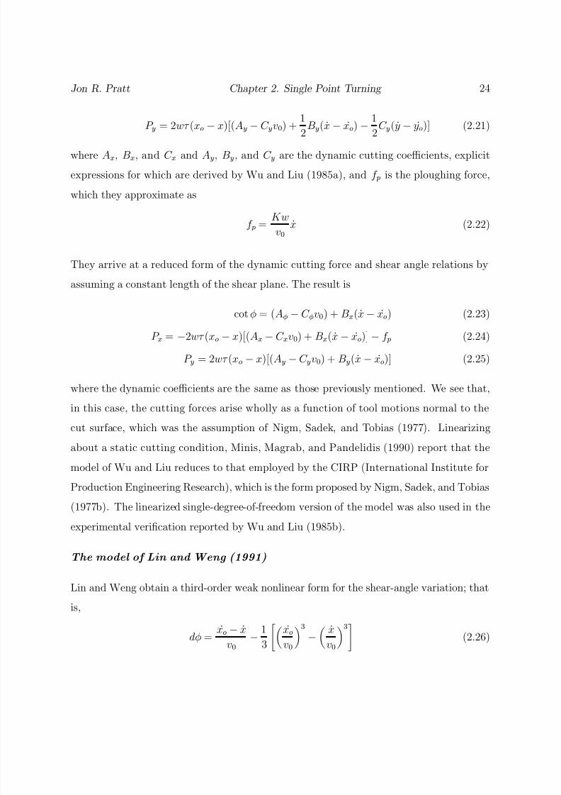
Jon R. Pratt Chapter 2. Single Point Turning 24
P y = 2wτ (xo − x)[(Ay − C yv0) + 1
2By(x − xo) −
1
2C y(y − yo)] (2.21)
where Ax, Bx, and C x and Ay, By, and C y are the dynamic cutting coefficients, explicit
expressions for which are derived by Wu and Liu (1985a), and f p is the ploughing force,
which they approximate as
f p = Kw
v0x (2.22)
They arrive at a reduced form of the dynamic cutting force and shear angle relations by
assuming a constant length of the shear plane. The result is
cot φ = (Aφ − C φv0) + Bx(x− xo) (2.23)
P x = −2wτ (xo − x)[(Ax − C xv0) + Bx(x − xo)]− f p (2.24)
P y = 2wτ (xo − x)[(Ay − C yv0) + By(x − xo)] (2.25)
where the dynamic coefficients are the same as those previously mentioned. We see that,
in this case, the cutting forces arise wholly as a function of tool motions normal to the
cut surface, which was the assumption of Nigm, Sadek, and Tobias (1977). Linearizing
about a static cutting condition, Minis, Magrab, and Pandelidis (1990) report that the
model of Wu and Liu reduces to that employed by the CIRP (International Institute for
Production Engineering Research), which is the form proposed by Nigm, Sadek, and Tobias
(1977b). The linearized single-degree-of-freedom version of the model was also used in the
experimental verification reported by Wu and Liu (1985b).
The model of Lin and Weng (1991)
Lin and Weng obtain a third-order weak nonlinear form for the shear-angle variation; that
is,
dφ = xo − x
v0−
1
3
xo
v0
3
−
x
v0
3
(2.26)

8/13/2019 Vibration Control for Chatter Suppression with Application to Boring Bars
http://slidepdf.com/reader/full/vibration-control-for-chatter-suppression-with-application-to-boring-bars 46/193
Jon R. Pratt Chapter 2. Single Point Turning 25
Then they expand Eqs. (2.1) and (2.2) about the mean shear angle φo and obtain
F x(φo + dφ) = F x(φo) +
∂F x∂φ
φo
dφ +
∂ 2F x∂φ2
φo
dφ2 + ... (2.27)
F y(φo + dφ) = F y(φo) +
∂F y∂φ
φo
dφ +
∂ 2F y∂φ2
φo
dφ2 + ... (2.28)
Substituting Eq. (2.26) into Eqs. (2.27) and (2.28), taking the appropriate derivatives
while making use of the shear-angle relation
φ = C 1 − 1
2(β − α) (2.29)
and keeping terms up to third order, they obtain
dP x = Axw∆s − Bxws s
vo
+ ws
C x
s
vo
2
+ Bx
xo yo − xy
v2o
(2.30)
+ws
Bx
(x3
o − x3) − 3(xo y2o − xy2)
3v3o
− C x
2s( xo yo − xy)
v3o
− Dx
s
vo
3
dP y = Ayw∆s − Byws s
vo
+ ws
C y
s
vo
2
+ By
xo yo − xy
v2o
(2.31)
+ws
By(x3
o − x3) − 3(xoy2o − xy2)
3v3o− C y
2s( xo yo − xy)
v3o− Dy
s
vo
3where ∆s = s(t) − so, and s(t) = xo − x.
We see that, to the second-order approximation, these equations have the form employed
by Wu and Liu (1985a)).
The model of Grabec (1988)
Grabec uses empirical relations derived from the work of Hastings, Oxley, and Stevenson(1971) and Hastings, Mathew, and Oxley (1980) to develop dynamic cutting-force relations.
First, the thrust force F x is related to the main cutting force F y through a friction coefficient
K as
F x = K F y (2.32)
8/13/2019 Vibration Control for Chatter Suppression with Application to Boring Bars
http://slidepdf.com/reader/full/vibration-control-for-chatter-suppression-with-application-to-boring-bars 47/193
Jon R. Pratt Chapter 2. Single Point Turning 26
He considers the case where cuts do not overlap and models the main cutting force as a
function of the cutting speed v and chip thickness s in the form
F y = F yo
s
so
C 1
v
vo
− 12
+ 1
(2.33)
where F yo is the steady-state main cutting force at the nominal cutting condition. The
friction coefficient is treated in a similar fashion. The result is
K = K o
C 2
vf R
vo
− 12
+ 1
C 2
s
so
− 12
+ 1
(2.34)
where K o = F xo/F yo is a constant determined at the nominal cutting condition, vf is the
friction velocity or the velocity along the tool rake face, and ρ is the chip thickness ratio.
Grabec assumes also that the chip thickness ratio is a function of the cutting speed; that
is,
ρ(t) = ρo
C 4
v
vo
− 12
+ 1
(2.35)
Finally, he makes the following substitutions in order to obtain dynamic cutting relations:
s(t) = so − x(t), (2.36)
v(t) = vo − y(t), (2.37)
vf (t) = v(t)
ρt − y(t) (2.38)
The model of Moon (1994)
Moon assumes that a shear-plane model is applicable and writes
F x = N sin α − F cos α (2.39)
F = µN (2.40)

8/13/2019 Vibration Control for Chatter Suppression with Application to Boring Bars
http://slidepdf.com/reader/full/vibration-control-for-chatter-suppression-with-application-to-boring-bars 48/193
8/13/2019 Vibration Control for Chatter Suppression with Application to Boring Bars
http://slidepdf.com/reader/full/vibration-control-for-chatter-suppression-with-application-to-boring-bars 49/193
Jon R. Pratt Chapter 2. Single Point Turning 28
gives rise to terms that are linear in the chip-thickness modulation ds. The penetration, or
ploughing effect, produces a damping-type force proportional to the tool oscillation normal
to the work surface. Finally, the oscillation of the shear plane leads to nonlinear terms that
are proportional to the product of the chip thickness and its derivative. Oscillation of the
shear plane is also responsible for coupling the main and thrust cutting forces.
2.3 Cutting Stability for Simple Machine-Tool Struc-
tures
The dynamic forces that arise during cutting can cause the machine-tool structure to loose
stability. When this happens, the machine-tool vibrates and is said to chatter. Chatter
occurs at the point when relative motion between the tool and workpiece results in a
negative damping force that overcomes the dissipation inherent in the system. Chatter is a
so-called self-excited oscillation because the energy that creates the vibration is generated
by the vibration itself.
In this section, we consider the stability of a flexible tool in the presence of a dynamic
cutting force
dP = wk1
ds +
2πC 1Ω
x + 2πC 2
Ω ds
(2.43)
where w is the width of cut, k1 is the “chip thickness coefficient”, C 1 = K/k1 and K is the
“penetration rate coefficient”, C 2 is a cutting-force constant, and x is the tool displacment
normal to the machined surface in an orthogonal cutting geometry. This is the model
considered by Nigm, Sadek, and Tobias (1977) and has the same form as the linearized
model of Wu and Liu (1986b) and Lin and Weng (1991). The cutting force is seen to
depend on the chip-thickness modulation ds, its derivative ds, and the penetration rate x.

8/13/2019 Vibration Control for Chatter Suppression with Application to Boring Bars
http://slidepdf.com/reader/full/vibration-control-for-chatter-suppression-with-application-to-boring-bars 50/193
Jon R. Pratt Chapter 2. Single Point Turning 29
2.3.1 Stability of a Single-Degree-of-Freedom Cutting Model
In many practical instances, the structural modes of vibration of the machine tool are well
spaced and may be considered as separate, single-degree-of-freedom linear oscillators. A
modal approximation for the receptance of such a structure can be formulated as (Ewins,
1986)
Gab(ω) =hnω2n
(1 − ω2/ω2n) + j(2ζ nω/ωn)
+ C (2.44)
where ωn, ζ , and hn are the natural frequency, damping, and modal factor, respectively,
and C is a constant representing the contribution of higher modes. The receptance Gab
characterizes the response of the structure in the a direction to a force in the b direction.
Now consider the system of Fig. 2.7, which is an example taken from Tlusty (1985). Tlusty
observes that only the projection P cos (θ − ψ) of the cutting force acts in the principal
modal coordinate X . Furthermore, only the projection x cos ψ of the vibration of the
mode in the direction X will modulate the chip, hence
Gxx = X (ω)
P (ω) =
X (ω)
P (ω) cos(θ − ψ)cos ψ = uGxx (2.45)
where u = cos (θ − ψ)cos ψ is the directional factor of the mode and Gxx is the so-called
oriented transfer function or operative receptance locus.
The response of the machine tool to a harmonic cutting force dP (ω) in a direction normal
to the machined surface is
X (ω) = Gxx(ω)dP (ω) (2.46)
To assess the stability using the operative receptance locus, we assume that the cutting
process has been disturbed, causing tool oscillations x(t) to be superimposed on the steady
feed so normal to the machined surface. The material was machined on a previous tool
8/13/2019 Vibration Control for Chatter Suppression with Application to Boring Bars
http://slidepdf.com/reader/full/vibration-control-for-chatter-suppression-with-application-to-boring-bars 51/193
Jon R. Pratt Chapter 2. Single Point Turning 30
X
X '
ψ
θ
k
cmP
Figure 2.7: Single-degree-of-freedom tool.
pass, which left a wavy surface that is the outer chip modulation xo(t). The instantaneous
chip thickness is thus
s(t) = xo(t) − x(t) (2.47)
We are interested in determining the point where the system becomes marginally stable.
At this threshold, we assume that the system oscillates freely at the chatter frequency ωc
so that
x(t) = ao cos(ωct) (2.48)
xo(t) = ao cos(ωct − β ) + so (2.49)
where β is the phase angle between the inner and outer chip modulations. For a single-point
turning operation,
β = 2πωc
Ω (2.50)
8/13/2019 Vibration Control for Chatter Suppression with Application to Boring Bars
http://slidepdf.com/reader/full/vibration-control-for-chatter-suppression-with-application-to-boring-bars 52/193
Jon R. Pratt Chapter 2. Single Point Turning 31
where Ω is the spindle rotational speed in rad/s.
The variation of the chip thickness is
ds = s(t)− so = Ax(t) + B
ωc
x(t) (2.51)
and the derivative of its variation is
ds = s = Ax(t)− ωcBx(t) (2.52)
where
A = cos (β )− 1 (2.53)
B = − sin(β ) (2.54)
Substituting the expressions for the chip thickness and its derivative into the incremental
cutting force
dP = wk1
(A − βC 2B)x(t) +
2π
Ω (C 1 + C 2A) +
B
ωc
x(t)
(2.55)
we see that the cutting force acts in such a fashion as to produce both displacement and
velocity feedback to the machine-tool structure.
For the single-degree-of-freedom problem
Gxx = u1
m
ω2n − ω2
c + i2ζωcωn
(2.56)
We let dP (t) = dP (ωc)eiωct and x(t) = X (ωc)eiωct and substitute Eqs. (2.55) and (2.56)
into Eq. (2.46). Then, separating real and imaginary terms, we obtain the linear stability
condition
ω2n − ω2
c − uwk1
m (A− βC 2B) = 0 (2.57)
2ζωcωn − uwk1
m
2π
Ω (C 1 + C 2A) +
B
ωc
= 0 (2.58)
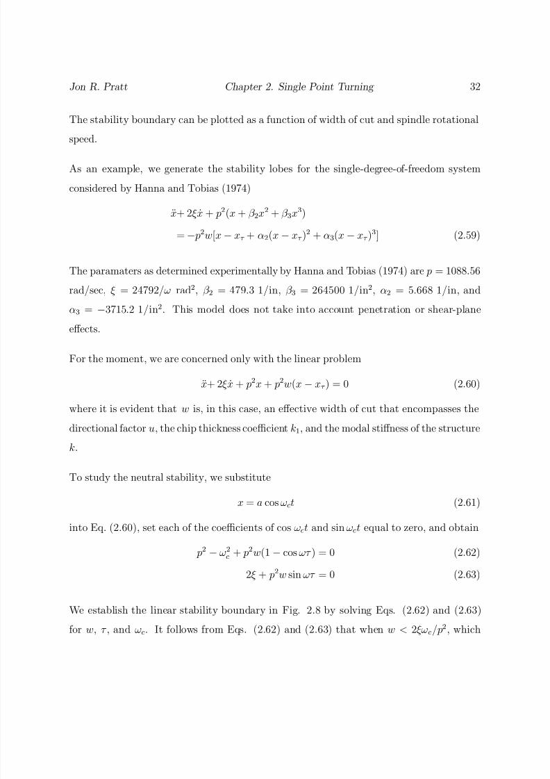
8/13/2019 Vibration Control for Chatter Suppression with Application to Boring Bars
http://slidepdf.com/reader/full/vibration-control-for-chatter-suppression-with-application-to-boring-bars 53/193
Jon R. Pratt Chapter 2. Single Point Turning 32
The stability boundary can be plotted as a function of width of cut and spindle rotational
speed.
As an example, we generate the stability lobes for the single-degree-of-freedom system
considered by Hanna and Tobias (1974)
x+ 2ξ x + p2(x + β 2x2 + β 3x3)
=− p2w[x− xτ + α2(x − xτ )2 + α3(x − xτ )
3] (2.59)
The paramaters as determined experimentally by Hanna and Tobias (1974) are p = 1088.56rad/sec, ξ = 24792/ω rad2, β 2 = 479.3 1/in, β 3 = 264500 1/in2, α2 = 5.668 1/in, and
α3 = −3715.2 1/in2. This model does not take into account penetration or shear-plane
effects.
For the moment, we are concerned only with the linear problem
x+ 2ξ x + p2x + p2w(x − xτ ) = 0 (2.60)
where it is evident that w is, in this case, an effective width of cut that encompasses the
directional factor u, the chip thickness coefficient k1, and the modal stiffness of the structure
k.
To study the neutral stability, we substitute
x = a cos ωct (2.61)
into Eq. (2.60), set each of the coefficients of cos ωct and sin ωct equal to zero, and obtain
p2 − ω2c + p2w(1 − cos ωτ ) = 0 (2.62)
2ξ + p2w sin ωτ = 0 (2.63)
We establish the linear stability boundary in Fig. 2.8 by solving Eqs. (2.62) and (2.63)
for w, τ , and ωc. It follows from Eqs. (2.62) and (2.63) that when w < 2ξωc/p2, which

8/13/2019 Vibration Control for Chatter Suppression with Application to Boring Bars
http://slidepdf.com/reader/full/vibration-control-for-chatter-suppression-with-application-to-boring-bars 54/193
Jon R. Pratt Chapter 2. Single Point Turning 33
is 0.0418, the cutting process remains stable. We note that this occurs when the phasing
between subsequent cuts is β = ωcτ = 2nπ + 3π/2 where n = 1, 2, 3, · · ·.
The line w = 0.0418 on the stability plot is known as the tangent boundary to the lobed
stability curve. This tangent boundary takes on different shapes as we include the effects
of the penetration rate and shear plane-oscillations. Tobias (1965) shows that, as the
cutting speed is increased, the tangent boundary asymptotically approaches the straight
line boundary, even if one considers the effects of both positive and negative penetration-
rate coefficients.
τ
Figure 2.8: Stability lobes for the model of Hanna and Tobias (1974).
Wu and Liu (1986b) explored the effect of shear-plane oscillations in addition to the
penetration rate on the tangent boundary. Using energy considerations they show that
β = ωcτ = 2nπ + 3π/2 where n = 1, 2, 3 . . . is the approximate phasing between the inner
and outer chip modulations along the tangent boundary to the lobed stability curves. They
then solve for w as a function of the rotational speed Ω along the tangent boundary. They
find that the penetration effect tends to have a stabilizing influence at low cutting speeds,
whereas friction along the rake face tends to have a destabilizing influence. Both effects

8/13/2019 Vibration Control for Chatter Suppression with Application to Boring Bars
http://slidepdf.com/reader/full/vibration-control-for-chatter-suppression-with-application-to-boring-bars 55/193
8/13/2019 Vibration Control for Chatter Suppression with Application to Boring Bars
http://slidepdf.com/reader/full/vibration-control-for-chatter-suppression-with-application-to-boring-bars 56/193
Jon R. Pratt Chapter 2. Single Point Turning 35
Gx2x2(ω) =
h2ω2
2
(1 − ω2/ω22) + j(2ζ 2ω/ω2) + C 2 (2.65)
where ωn, ζ n, and hn are the natural frequency, damping, and modal factor, respectively, of
mode n, and C n is a constant representing the contribution of higher modes to mode n. The
directional factors are computed by taking a unit cutting force vector dP and projecting it
onto X 1 and X 2 and finally onto X . The result is
u1 = cos (θ − ψ1)cos ψ1 (2.66)
u2 = − cos(
1
2π + ψ1 − θ)sin ψ1 (2.67)
The operative response locus is then
Gxx = u1Gx1x1 + u2Gy2y2 (2.68)
For the simplest regenerative cutting condition,
dP (t) = −k1[w(x(t)− x(t− τ ))] (2.69)
The stability is determined as before. Let dP (t) = dP (ωc)eiωct and x(t) = X (ωc)eiωct in
Eq. (2.69) and substitute Eqs. (2.68) and (2.69) into Eq. (2.46). Then, by separting real
and imaginary parts, the characteristic equation of the system.
It is well-known that the stability of a system with two orthogonal modes is strongly
dependent on the orientation of these modes (Tlusty, 1985; Tobias, 1965) with respect to
the machined surface. For instance, if ψ1 = 0 then the linear stability is determined wholly
by the stability of the mode normal to the machined surface. The result is quite different,
however, if the principal modal coordinates are rotated with respect to the normal to the
machined surface, as shown by Kuchma (1957) who performed tests using boring bars of
nonuniform cross-section to reveal this dependence.
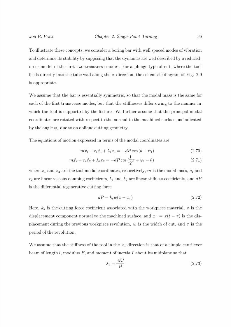
8/13/2019 Vibration Control for Chatter Suppression with Application to Boring Bars
http://slidepdf.com/reader/full/vibration-control-for-chatter-suppression-with-application-to-boring-bars 57/193
Jon R. Pratt Chapter 2. Single Point Turning 36
To illustrate these concepts, we consider a boring bar with well spaced modes of vibration
and determine its stability by supposing that the dynamics are well described by a reduced-
order model of the first two transverse modes. For a plunge type of cut, where the tool
feeds directly into the tube wall along the x direction, the schematic diagram of Fig. 2.9
is appropriate.
We assume that the bar is essentially symmetric, so that the modal mass is the same for
each of the first transverse modes, but that the stiffnesses differ owing to the manner in
which the tool is supported by the fixture. We further assume that the principal modal
coordinates are rotated with respect to the normal to the machined surface, as indicated
by the angle ψ1 due to an oblique cutting geometry.
The equations of motion expressed in terms of the modal coordinates are
m x1 + c1 x1 + λ1x1 = −dP cos (θ − ψ1) (2.70)
m x2 + c2 x2 + λ2x2 = −dP cos (1
2π + ψ1 − θ) (2.71)
where x1 and x2 are the tool modal coordinates, respectively, m is the modal mass, c1 andc2 are linear viscous damping coefficients, λ1 and λ2 are linear stiffness coefficients, and dP
is the differential regenerative cutting force
dP = ksw(x − xτ ) (2.72)
Here, ks is the cutting force coefficient associated with the workpiece material, x is the
displacement component normal to the machined surface, and xτ = x(t − τ ) is the dis-
placement during the previous workpiece revolution, w is the width of cut, and τ is the
period of the revolution.
We assume that the stiffness of the tool in the x1 direction is that of a simple cantilever
beam of length l, modulus E , and moment of inertia I about its midplane so that
λ1 = 3EI
l3 (2.73)

8/13/2019 Vibration Control for Chatter Suppression with Application to Boring Bars
http://slidepdf.com/reader/full/vibration-control-for-chatter-suppression-with-application-to-boring-bars 58/193
Jon R. Pratt Chapter 2. Single Point Turning 37
Dividing through by the modal mass m, we obtain
x1 + 2ζ 1ω1 x1 + ω21x1 = −dP
ω21
λ1cos(θ − ψ1) (2.74)
x2 + 2ζ 2ω2 x2 + ω22x2 = dP
ω21
λ1sin(θ − ψ1) (2.75)
where ζ 1 and ζ 2 are linear viscous damping ratios, and ω1 and ω2 are the natural frequencies.
¿From Fig. 2.9 we find that
x = x1 cos(ψ1) − x2 sin(ψ1) (2.76)
so that
dP = ksw[cos(ψ1)(x1 − x1τ ) − sin(ψ1)(x2 − x2τ )] (2.77)
Let γ 1 = ω21
ksλ1
cos(θ − ψ1), γ 2 = −ω21
ksλ1
sin(θ − ψ1), η = cos (ψ1), and ν = − sin(ψ1), then
the equations of motion can be rewritten as
x1 + 2ζ 1ω1 x1 + ω21x = −γ 1w[η(x1 − x1τ ) + ν (x2 − x2τ )] (2.78)
x2 + 2ζ 2ω2 x1 + ω22x = −γ 2w[η(x1 − x1τ ) + ν (x2 − x2τ )] (2.79)
To analyze the stability of this system, we assume zero initial conditions, take the Laplace
transform, and obtain
(s2 + 2ζ 1ω1s + ω21)X 1(s) = −γ 1w[η(1 − e−sτ )X 1(s) + ν (1 − e−sτ )X 2(s)] (2.80)
(s2 + 2ζ 2ω2s + ω22)X 2(s) = −γ 2w[η(1 − e−sτ )X 1(s) + ν (1 − e−sτ )X 2(s)] (2.81)
Then, solving Eq. (2.81) for X 2(s) yields
X 2(s) = −γ 2wη(1− e−sτ )X 1(s)
s2 + 2ζ 2ω2s + ω22 + γ 2wν (1 − e−sτ )
(2.82)
8/13/2019 Vibration Control for Chatter Suppression with Application to Boring Bars
http://slidepdf.com/reader/full/vibration-control-for-chatter-suppression-with-application-to-boring-bars 59/193
Jon R. Pratt Chapter 2. Single Point Turning 38
Substituting Eq. (2.82) into Eq. (2.80), we find the characteristic equation
[s2 + 2ζ 1ω1s + ω21 + γ 1wη(1 − e−sτ )][s2 + 2ζ 2ω2s + ω2
2 + γ 2wν (1 − e−sτ )]
−γ 1γ 2w2ην (1 − e−sτ )2 = 0 (2.83)
To obtain the familiar lobed stability boundary, we assume s = iωc, separate real and
imaginary terms, and solve the resulting pair of equations for w and ωc as a function of the
delay τ .
We now consider the predicted cutting stability when the modal properties are f 2 = 493Hz and ζ 2 = 0.03 and f 1 = 365 Hz and ζ 1 = 0.02.
The boring bar itself is approximated as a circular cylinder of length 9 (length of bar
measured from tool tip to clamped end) and diameter 1. We recall that the moment
of inertia for a circular cross section is I = π/4(d/2)4, then λ1 = 6060 psi for a steel of
modulus E = 30000 kpsi. A represenative value for the cutting stiffness of aluminum is
ks = 145000 psi according to Kalpakjian (1992).
We consider two cases. The first case is a two-degree-of-freedom system where ψ1 = 15.
In the second case, ψ1 = 0 and the stability reduces to that of a single-degree-of-freedom
system. The resulting stability lobes are plotted for a range of spindle speeds around 170
rpm in Fig. 2.10. We see from the plot that the stability is affected by the presence of the
second degree of freedom.

8/13/2019 Vibration Control for Chatter Suppression with Application to Boring Bars
http://slidepdf.com/reader/full/vibration-control-for-chatter-suppression-with-application-to-boring-bars 60/193
Jon R. Pratt Chapter 2. Single Point Turning 39
2.80 2.84 2.88 2.92
1/τ
0.002
0.0022
0.0024
0.0026
w
Single-degree-of-freedom m odel
Two-degree-of-freedom model
Figure 2.10: Stability lobes for two-degree-of-freedom cutting system.

8/13/2019 Vibration Control for Chatter Suppression with Application to Boring Bars
http://slidepdf.com/reader/full/vibration-control-for-chatter-suppression-with-application-to-boring-bars 61/193
Chapter 3
A Linear Chatter Control Scheme
The linear stability of regenerative chatter was shown in Chapter 2 to be a complex function
of workpiece revolutions per minute and depth of cut for a fixed feedrate. We saw that
the maximum stable width of cut was directly related to the amount of positive damping
in the machine-tool structure for a fixed feedrate and cutting speed. Thus, the greaterthe damping in the system is, the larger the region is of stable machining operations.
Introducing some terminology from nonlinear dynamics, we refer to the transition from
static machining to chatter as a bifurcation. Thus, the stability diagram developed in
Chapter 2, or stability lobes as they are often referred to in the literature, represents the
locus of the bifurcation points encountered for a fixed feedrate as the speed and depth of
cut are allowed to vary. Our goal for a linear control system is to delay the onset of these
bifurcations. In other words, we seek to alter the system dynamics such that the stabilitylobes are shifted up and bifurcation occurs at larger depths of cut.
In this chapter we develop a vibration control system to enhance the tool damping and
thereby shift the stability lobes. To begin, we briefly consider some of the available control
40
8/13/2019 Vibration Control for Chatter Suppression with Application to Boring Bars
http://slidepdf.com/reader/full/vibration-control-for-chatter-suppression-with-application-to-boring-bars 62/193
Jon R. Pratt Chapter 3. Linear Chatter Control 41
options and settle on second-order feedback compensation, in essence an active vibration
absorber. We then take up the topic of active vibration absorbers for vibration control,
comparing and contrasting semi-active and fully active approaches and reviewing the for-
mulations found in the literature. Next, we consider the effect of an absorber on the
stability of the single-degree-of-freedom model for machine-tool dynamics that was ana-
lyzed in Chapter 2. We find that an absorber is quite effective in shifting the bifurcation
in the single-degree-of-freedom case.
3.1 Selecting a Vibration Control Strategy
Our goal for the boring-bar application is to achieve stable cuts while accomodating long
tool overhangs. It is clear that in order to achieve this goal we must enhance the tool’s
dynamic stiffness and damping. Obviously, we may achieve this via a number of meth-
ods. In this section we briefly review some of the known options and present the design
considerations that lead to our choice of 2nd-order feedback compensation.
3.1.1 Passive Vibration Control Solutions
Passive vibration control is achieved by incorporating design elements such as damping
materials and tuned mass absorbers into a structure to modify its response to initial con-
ditions and/or forced excitations. The phrase passive control arises because no external
energy source is associated with its operation. Passive methods have been, and continue to
be, the dominant choice for attacking vibration problems because of there simplicity and
economy.
For boring bars, one course of action, common on the shop floor, is to add a damping

8/13/2019 Vibration Control for Chatter Suppression with Application to Boring Bars
http://slidepdf.com/reader/full/vibration-control-for-chatter-suppression-with-application-to-boring-bars 63/193

8/13/2019 Vibration Control for Chatter Suppression with Application to Boring Bars
http://slidepdf.com/reader/full/vibration-control-for-chatter-suppression-with-application-to-boring-bars 64/193
Jon R. Pratt Chapter 3. Linear Chatter Control 43
mamoto, and Mizumoto (1989) used piezoelectric actuators to apply control moments to
the boring bar. Their system uses time delay to phase shift an accelerometer signal and
achieve narrowband velocity feedback control. In this way, they were able to add damping
to the first bending mode in a direction normal to the cutting surface. Tewani, Rouch,
and Walcott (1995) mounted a piezoelectric reaction mass actuator in the bar itself and
created what they termed an active dynamic absorber. Using optimal control methods,
they designed a feedback control system to add damping to the bar. The orientation of the
actuator in this scheme may be adjusted so that control forces are oriented in the plane of
chatter. We point out that the cutting force direction and the direction of chatter do not
necessarily coincide and that the direction of the cutting force vector can vary as a function
of time under dynamic cutting conditions.
¿From a structural viewpoint, a boring bar is simply a cantilevered beam, and one can
find examples of various active control schemes for this type of elements in the literature.
Our performance goal is to enhance the damping of targeted vibration modes. Robust and
efficient methods for this type of control, such as the positive position feedback of Goh
and Caughey (1985) and the active vibration absorber of Juang and Phan (1992), already
exist in the literature. In the remainder of this chapter we adapt these techniques to the
boring-bar chatter problem.
3.2 Vibration Absorption via 2nd-Order Compensators
For our purposes, vibration-absorber control strategies may be described as either passive,
or semiactive, or fully active, the distinction being made according to how the actuators and
sensors are used. We assume that the reader is familiar with passive absorption techniques
and proceed to describe some of the relevant active schemes.

8/13/2019 Vibration Control for Chatter Suppression with Application to Boring Bars
http://slidepdf.com/reader/full/vibration-control-for-chatter-suppression-with-application-to-boring-bars 65/193

8/13/2019 Vibration Control for Chatter Suppression with Application to Boring Bars
http://slidepdf.com/reader/full/vibration-control-for-chatter-suppression-with-application-to-boring-bars 66/193
Jon R. Pratt Chapter 3. Linear Chatter Control 45
variable feedback, many authors have also suggested the use of second-order compensators
in the feedback loop.
Lee and Sinha (1986) used full state-variable feedback and added an undamped second-
order feedback compensator, called a “disturbance accommodating controller” by Johnson
(1970, 1971), to achieve what they termed an active vibration absorber. Juang and Phan
(1992) developed a methodology for robust controller design for second-order dynamic
systems that also uses second-order feedback compensation. The positive-position-feedback
control of Goh and Caughey (1985) and Fanson and Caughey (1987) is yet another example
of second-order compensation for structural control.
We observe that these fully active control schemes do not require a physical absorber but
instead achieve a similar result via 2nd-order feedback compensation. The compensator is
a “virtual absorber”, to borrow the terminology of Juang and Phan (1992), and, as such,
its “virtual” mass, stiffness, and damping are at the user’s discretion. These methods are
fairly robust in the presence of uncertain plant dynamics, are easily designed using root-
locus techniques, and can be made immune to spillover effects provided that the actuator
and sensor are collocated, a topic we will take up again later. They may be implemented
using either digital or analog control. In digital control, the “virtual absorber” is simply
a second-order difference equation or an infinite impulse response digital filter. For analog
systems, a resonant second-order compensator circuit will suffice.
3.3 Application to Chatter Control
Mathematically, as in Chapter 2, we consider a structural model similar to that of Hanna
and Tobias (1974). Thus, we consider:
x + 2ξ x + p2(x + β 2x2 + β 3x3) = d(t) + f c(t) (3.1)

8/13/2019 Vibration Control for Chatter Suppression with Application to Boring Bars
http://slidepdf.com/reader/full/vibration-control-for-chatter-suppression-with-application-to-boring-bars 67/193

8/13/2019 Vibration Control for Chatter Suppression with Application to Boring Bars
http://slidepdf.com/reader/full/vibration-control-for-chatter-suppression-with-application-to-boring-bars 68/193
8/13/2019 Vibration Control for Chatter Suppression with Application to Boring Bars
http://slidepdf.com/reader/full/vibration-control-for-chatter-suppression-with-application-to-boring-bars 69/193
Jon R. Pratt Chapter 3. Linear Chatter Control 48
in the actual experimental system.
3.3.1 Linear Machine-Tool Stability Analysis with an Absorber
In this section we consider the stability of the machine tool model of Hanna and Tobias
(1974) with the addition of a fully-active vibration absorber. Thus, our complete system
may be described by
x + 2ξ x + p2(x + β 2x2 + β 3x3) = − p2w[x − xτ + α2(x− xτ )2 + α3(x − xτ )3]
+d(ca y + ω2ay) (3.11)
y + cay + ω2ay = −cx (3.12)
where all variables are as previously defined. Linearizing, we obtain
x + 2ξ x + p2x = − p2w(x − xτ ) + d(ca y + ω2ay) (3.13)
y + cay + ω2ay = −cx (3.14)
To design the absorber, we neglect the regenerative terms and note that the resulting system
is entirely analogous to a passive vibration absorber, as in Bruner et al (1992). It can be
shown that for c = 1, the controller gain d takes on the role of an effective mass ratio
d = ma/M if one considers y as the relative motion between a single-degree-of-freedom
plant of mass M and a damped vibration absorber of mass ma. In practice, the value
of d will be constrained by the limitations of the actuator system. For our purposes, we
chose d = 0.35 because it gave reasonable results for the scaling limitations of subsequent
analog-computer simulations.
Having fixed the effective mass ratio, one can use the design criteria of Den Hartog (1985)
to arrive at a frequency and damping for the absorber. According to Den Hartog, the
8/13/2019 Vibration Control for Chatter Suppression with Application to Boring Bars
http://slidepdf.com/reader/full/vibration-control-for-chatter-suppression-with-application-to-boring-bars 70/193
Jon R. Pratt Chapter 3. Linear Chatter Control 49
frequency ratio f = ωa/p that will produce an “optimal” absorber is
f = 1
1 + d (3.15)
while the absorber damping should be
ζ a =
3d
8(1 + d)3 (3.16)
Thus, for d = 0.35 the design parameters according to Den Hartog’s method are ωa/p = 0.74
and ζ = 0.23. We find through trial and error using an analog simulator that a frequency
ratio of ωa/p = 0.7 and an absorber damping factor of ca = 2ζ aωa where ζ a = 0.57 produce
a satisfactory frequency-response curve. The frequency ratio is in near agreement with the
design value while the damping is substantially higher than suggested. The discrepancy
in damping is not wholly unexpected since Den Hartog assumed that the damping of the
primary structure was negligible.
We now consider the stability of the controlled system in the presence of the regenerative
terms. To begin, we take the Laplace transform of Eqs. (3.13) and (3.14), assume zeroinitial conditions, and obtain
(s2 + 2ξs + p2 + p2w(1 − e−sτ ))X (s) = d(cas + ω2a)Y (s) (3.17)
(s2 + 2cas + ω2a)Y (s) =−s2X (s) (3.18)
Solving for Y (s) in terms of X (s) yields
Y (s) = −s2X (s)
s2 + 2ca
s + ω2
a
(3.19)
Substituting Eq. (3.19) into Eq. (3.17), we obtain the characteristic equation of the system
as
s4+ (2ξ + ca(1 + d))s3 + [ p2(1 + w(1 − e−sτ )) + 2ξca + ω2a(1 + d)]s2
+ [ca p2(1 + w(1− e−sτ )) + 2ξω2
a]s + ω2a p
2(1 + w(1 − e−sτ )) = 0 (3.20)

8/13/2019 Vibration Control for Chatter Suppression with Application to Boring Bars
http://slidepdf.com/reader/full/vibration-control-for-chatter-suppression-with-application-to-boring-bars 71/193
Jon R. Pratt Chapter 3. Linear Chatter Control 50
40.00 50.00 60.00 70.00 80.00
0.00
0.20
0.40
0.60
w
Figure 3.2: Linear stability diagram showing the critical width of cut as a function of the
rotational frequency. The upper curve corresponds to the controlled system and the lower
curve corresponds to the uncontrolled system.
We establish the linear stability boundary by substituting s = iω into Eq. (3.20), separating
real and imaginary parts, and solving the resulting pair of equations for w, τ , and ω. Using
the parameter values from Hanna and Tobias (1974) and letting d = 0.35, ωa/p = 0.7, and
ζ = 0.57, we plot the limit width of cut with and without the absorber as a function of the
time delay in Fig. 3.2. Clearly, the absorber has substantially increased the limit width of
cut.

8/13/2019 Vibration Control for Chatter Suppression with Application to Boring Bars
http://slidepdf.com/reader/full/vibration-control-for-chatter-suppression-with-application-to-boring-bars 72/193
Chapter 4
Control-System Hardware Design,
Integration, and Modeling
Having established that an absorber type control approach can improve cutting stability,
we design a prototype system for a specific boring bar and engine lathe setup. A model forthe prototype is generated using experimental modal analysis techniques. The frequency-
response characteristics of individual control elements are examined and used to build a
block diagram that yields the open-loop response of the actuator/sensor pairs. We find from
the structure of the plant frequency-response function characterizing an actuator/sensor
pair that the system is not collocated. Actuator impedance effects must be accounted for. A
third-order compensator is suggested and a single-degree-of-freedom design methodology is
presented for selecting controller gains. Good agreement between modeling and experimentis obtained.
51
8/13/2019 Vibration Control for Chatter Suppression with Application to Boring Bars
http://slidepdf.com/reader/full/vibration-control-for-chatter-suppression-with-application-to-boring-bars 73/193
Jon R. Pratt Chapter 4. Control System Hardware 52
4.1 Design Criteria
¿From a structural control viewpoint, the boring bar is a cantilevered beam. It has lateral
vibration modes in two orthogonal directions and is subject to disturbances in the form
of cutting forces at its free end that can couple these two coordinates, as we observed in
Chapter 2.
¿From Chapter 2, we also know that it is a common assumption in cutting force analysis
that the shearing of material from the workpiece occurs along a thin plane. When this isthe case, the resultant cutting force is planar with a magnitude dependent on the variation
of the chip thickness. This is the so-called dynamic orthogonal cutting condition. Based
on the assumption of dynamic orthogonal cutting, an argument can be made that it is
only necessary to control the tool motion in the direction perpindicular to the machined
surface, because these motions modulate the chip thickness. This notion is embedded in
the determination of an operative receptance locus to assess machine-tool stability and is a
guiding design principle in the single-axis, semi-active vibration-absorber scheme that was
developed and used by Tewani, Walcott, and Rouch (1991) with success.
Orthogonal cutting with a single edge is seldom the case in practice, and it has been our ex-
perience that for shallow, finish type cuts, where chatter is most common and detrimental,
a complex oblique-cutting condition exists along multiple cutting surfaces. Furthermore,
it seems likely that, as the linear stability of cutting is extended by controlling tool mo-
tions normal to the machined surface, one is likely to encounter a destabilizing effect in
the uncontrolled coordinate due to shear-plane oscillation effects or plowing, even for an
orthogonal condition.
Consider the nonlinear model of Wu and Liu(1985 a) Eqs. (2.20) and (2.21). If we assume
that the motion normal to the machined surface is constrained by the control and that the
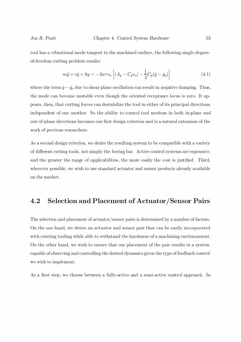
8/13/2019 Vibration Control for Chatter Suppression with Application to Boring Bars
http://slidepdf.com/reader/full/vibration-control-for-chatter-suppression-with-application-to-boring-bars 74/193
Jon R. Pratt Chapter 4. Control System Hardware 53
tool has a vibrational mode tangent to the machined surface, the following single-degree-
of-freedom cutting problem results:
my + cy + ky = −2wτ so
(Ay − C yvo) −
1
2C y(y − yo)
(4.1)
where the term y− yo due to shear plane oscillation can result in negative damping. Thus,
the mode can become unstable even though the oriented receptance locus is zero. It ap-
pears, then, that cutting forces can destabilize the tool in either of its principal directions
independent of one another. So the ability to control tool motions in both in-plane and
out-of-plane directions becomes our first design criterion and is a natural extension of the
work of previous researchers.
As a second design criterion, we desire the resulting system to be compatible with a variety
of different cutting tools, not simply the boring bar. Active control systems are expensive,
and the greater the range of applicabilities, the more easily the cost is justified. Third,
wherever possible, we wish to use standard actuator and sensor products already available
on the market.
4.2 Selection and Placement of Actuator/Sensor Pairs
The selection and placement of actuator/sensor pairs is determined by a number of factors.
On the one hand, we desire an actuator and sensor pair that can be easily incorporated
with existing tooling while able to withstand the harshness of a machining envirnonment.
On the other hand, we wish to ensure that our placement of the pair results in a system
capable of observing and controlling the desired dynamics given the type of feedback control
we wish to implement.
As a first step, we choose between a fully-active and a semi-active control approach. In
8/13/2019 Vibration Control for Chatter Suppression with Application to Boring Bars
http://slidepdf.com/reader/full/vibration-control-for-chatter-suppression-with-application-to-boring-bars 75/193
Jon R. Pratt Chapter 4. Control System Hardware 54
principle, one could design a bidirectional semi-active absorber system using two actuators
and appropriate sensors. Such a system would ideally be attached near the free end of the
bar to achieve the greatest mechanical advantage and hence controllability. This means
placing the actuators inside the tool to avoid interaction with the cutting process, as in
the system of Tewani, Walcott, and Rouch (1991). Such a strategy places severe geometric
constraints on the design, involves modifying the tool, and necessitates custom actuator
designs. For these reasons the approach was not considered for this Dissertation. Instead,
we elected to develop a fully-active scheme using actuators located near the tool base.
This removes the geometric constraints on actuator size, keeps the tool modifications to a
minimum, and facilitates the use of standard actuators.
A common approach for actuating a cantilevered beam near its base is to incorporate piezo-
electric benders, essentially the approach taken by Matsubara, Yamamoto, and Mizumoto
(1989). Such a solution has merit, but results in a custom, one size fits all tool. Rather
than creating such a specialized tool, we opted to create a special tool holder. In this
way, we could accomodate vibration control for other tooling. A schematic of the resulting
design is shown in Fig. 4.1.
In this first design iteration, the actuators are positioned so that they sting the tool near
the tool base. This sacrifices some potential tool overhang. In future work, we plan to
explore similar control using actuation nearer to the fixed boundary, thus maximizing the
usage of the tool.
At present, actuators available for structural control consist of electrodynamic, induced
strain (the so-called smart materials), and hydraulic or pneumatic types. Of these, the
hydraulic and pneumatic types have tremendous force and stroke capabilities but lack
sufficient bandwidth for effective chatter control. Electrodynamic actuators have sufficient
bandwidth and stroke, are inexpensive, and are a proven reliable technology. However,

8/13/2019 Vibration Control for Chatter Suppression with Application to Boring Bars
http://slidepdf.com/reader/full/vibration-control-for-chatter-suppression-with-application-to-boring-bars 76/193
Jon R. Pratt Chapter 4. Control System Hardware 55
Workpiece
BoringBar
+y
+x+zΩ
Cross SlideMotions
HorizontalActuator
VerticalActuator
ToolHolder
Dynamometer
MountingBlock
CrossSlide
Side View of ActuatorAssembly
Top View of ActuatorAssembly
VerticalAccelerometer
HorizontalAccelerometer
Insert
TensionedWire
Figure 4.1: Boring bar control system layout.
they tend to be more bulky than their induced strain counterparts for comparable force
capabilities. The force required to actuate the beam near its base is substantial while the
stroke required is small, so we chose to use induced strain actuators.
Of the available induced strain actuators, those fashioned from magnetostrictive materials,
such as Terfenol-D, have the advantage that they can be driven using standard audio-type
power amplifiers, because their electrical behavior is comparable to electrodynamic shak-
ers. Terfenol-D actuators in particular also have been shown to have a high energy density

8/13/2019 Vibration Control for Chatter Suppression with Application to Boring Bars
http://slidepdf.com/reader/full/vibration-control-for-chatter-suppression-with-application-to-boring-bars 77/193
Jon R. Pratt Chapter 4. Control System Hardware 56
in comparison to comparable piezoelectric stack-type actuators. And, in the author’s ex-
perience, Terfenol-D actuators are more rugged than piezo-stack actuators, because small
localized crack-type failures in the actuator material do not automatically render the ac-
tuator useless as is often the case in piezoceramic materials. Thus, we chose Terfenol-D
actuators for our prototype.
4.3 Description of the Smart-Tool System
The layout of components is shown in Fig. 4.1. The control system is comprised of two
actuator/sensor pairs; one pair is used to control motion in the direction normal to the
machined surface, the other pair is used to control motions in the direction tangential to
the machined surface.
The lathe used in this study is a 10-horsepower, Yamazaki Mazak, two-axis engine lathe
with a 14-inch four-jaw chuck. The tool is a 12-inch long and 1-inch diameter boring bar
with an ISO TNMG 160304 insert. The side rake angle is −5, the back rake angle is −12,
and the lead angle is 0. The bar is tapped with a series of 10/32 holes to accomodate the
attachment of actuators through flexural elements known as “stingers”. We note that the
orientation of the insert in the boring bar yields an oblique cutting geometry.
The tool holder is a custom designed clamp bolted to a dynamometer that is itself bolted
to a mounting block on the cross slide. The bar is overhung with a length-to-diameter ratio
of 8, as measured from the tool holder to the cutting edge, though the clamped length is
best approximated as 9 through consideration of the set screw location that holds the bar
in the tool holder.
Two ETREMA Products, Inc., 75/12 MP Terfenol-D actuators oriented in the x and y
8/13/2019 Vibration Control for Chatter Suppression with Application to Boring Bars
http://slidepdf.com/reader/full/vibration-control-for-chatter-suppression-with-application-to-boring-bars 78/193

8/13/2019 Vibration Control for Chatter Suppression with Application to Boring Bars
http://slidepdf.com/reader/full/vibration-control-for-chatter-suppression-with-application-to-boring-bars 79/193

8/13/2019 Vibration Control for Chatter Suppression with Application to Boring Bars
http://slidepdf.com/reader/full/vibration-control-for-chatter-suppression-with-application-to-boring-bars 80/193
Jon R. Pratt Chapter 4. Control System Hardware 59
-60
-40
-20
0
0.00 1000.00 2000.00 3000.00
-360
-180
0
180
Figure 4.3: Bode plot of the tangential plant response function. The dashed line is the
experimentally measured response while the solid line is obtained from the model.
forces. We develop a model for the tangential control loop as an example of the procedure.
The actuator is provided with a random voltage excitation and the corresponding output
acceleration is sensed as a voltage from the accelerometer signal conditioner. The actuator
power amplifier is set at a midrange gain and a random voltage input is selected to avoid
amplifier and actuator saturation. Both the input and output voltages are measured using
a digital frequency analyzer that computes the corresponding FRF, shown as the dashed
line in the Bode plot of Fig. 4.3.
The phase plot indicates first-order dynamics, as evidenced by the roll off from 180 to
approximately 90 between 0 and approximately 300 Hz. This is to be expected because
the actuator is magnetostrictive, and its electrical impedance should resemble that of an
inductive load. Between 450 and 600 Hz the response exhibits a resonance peak accompa-
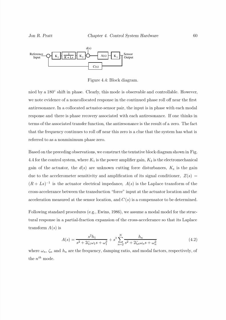
8/13/2019 Vibration Control for Chatter Suppression with Application to Boring Bars
http://slidepdf.com/reader/full/vibration-control-for-chatter-suppression-with-application-to-boring-bars 81/193
Jon R. Pratt Chapter 4. Control System Hardware 60
1R + Ls K2
d(s)
SensorOutput
ReferenceInput K1 K s
C(s)
A(s)
Figure 4.4: Block diagram.
nied by a 180 shift in phase. Clearly, this mode is observable and controllable. However,
we note evidence of a noncollocated response in the continued phase roll off near the first
antiresonance. In a collocated actuator-sensor pair, the input is in phase with each modal
response and there is phase recovery associated with each antiresonance. If one thinks in
terms of the associated transfer function, the antiresonance is the result of a zero. The fact
that the frequency continues to roll off near this zero is a clue that the system has what is
referred to as a nonminimum phase zero.
Based on the preceding observations, we construct the tentative block diagram shown in Fig.
4.4 for the control system, where K 1 is the power amplifier gain, K 2 is the electromechanical
gain of the actuator, the d(s) are unknown cutting force disturbances, K s is the gain
due to the accelerometer sensitivity and amplification of its signal conditioner, Z (s) =
(R + Ls)−1 is the actuator electrical impedance, A(s) is the Laplace transform of the
cross-accelerance between the transduction “force” input at the actuator location and the
acceleration measured at the sensor location, and C (s) is a compensator to be determined.
Following standard procedures (e.g., Ewins, 1986), we assume a modal model for the struc-
tural response in a partial-fraction expansion of the cross-accelerance so that its Laplace
transform A(s) is
A(s) = s2h1
s2 + 2ζ 1ω1s + ω21
+ s2N
n=2
hn
s2 + 2ζ nωns + ω2n
(4.2)
where ωn, ζ n and hn are the frequency, damping ratio, and modal factors, respectively, of
the nth mode.
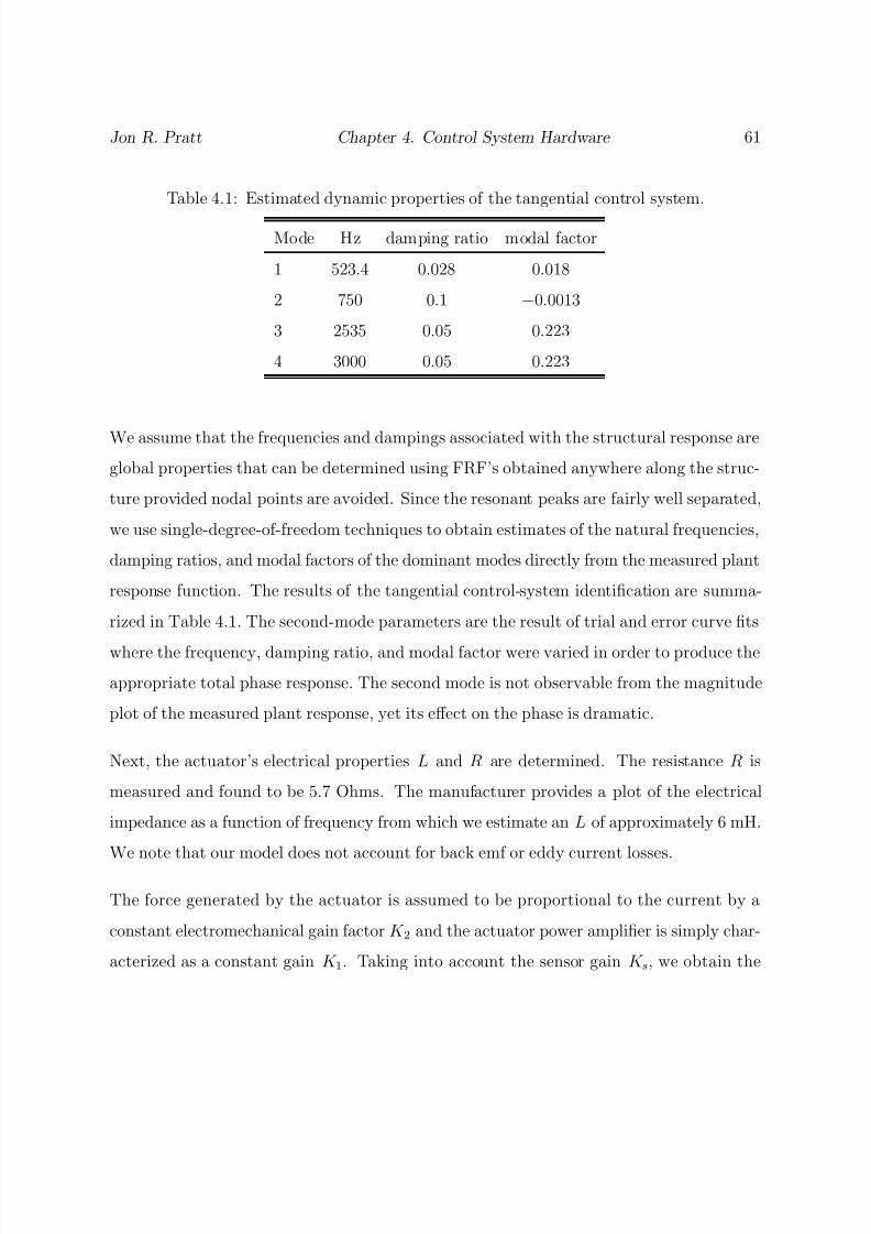
8/13/2019 Vibration Control for Chatter Suppression with Application to Boring Bars
http://slidepdf.com/reader/full/vibration-control-for-chatter-suppression-with-application-to-boring-bars 82/193

8/13/2019 Vibration Control for Chatter Suppression with Application to Boring Bars
http://slidepdf.com/reader/full/vibration-control-for-chatter-suppression-with-application-to-boring-bars 83/193
Jon R. Pratt Chapter 4. Control System Hardware 62
plant transfer function
V out(s)V in(s)
= K 1K 2K sZ (s)A(s) (4.3)
Rather than determine each of the gains separately, we lump them together as a single
parameter K . Setting K = 48 and letting s = iω, where ω is the frequency of excitation,
we plot the model plant response as the solid line in Fig. 4.3.
4.4.2 Closing the Loop
To achieve effective chatter control, we must minimize the tool vibratory response to ar-
bitrary disturbance forces. In terms of closed-loop performance goals, this translates into
an output regulation problem. However, there is little to be gained by controlling all of
the states, or modes, present in the plant response functions because the chatter vibra-
tion at the tool tip is clearly dominated by the first mode in each case. Thus we seek a
compensation scheme that targets this problematic mode for regulation.
Second-order compensators, as discussed in Chapter 3, have been proposed in the litera-
ture to provide loop-shaping control of structures (Goh and Caughey, 1985 ; Fanson and
Caughey, 1987; and Juang and Phan, 1992) using collocated sensor-actuator pairs. In these
approaches, the compensator is used to increase the damping of a targeted structural mode
in a fashion analogous to a mechanical vibration absorber. For a single-degree-of-freedom
structure, these controllers take the form
x + 2ζ 1ω1x + ω21x = d(t) + f c(y, y,x, x) (4.4)
y + 2ζ cωc y + ω2c y = C (y, y,x, y) (4.5)
where x is the generalized structural coordinate, y is the compensator coordinate with
damping factor ζ c and frequency ωc, and the coupling is defined by the functions C (y, y,x, x)
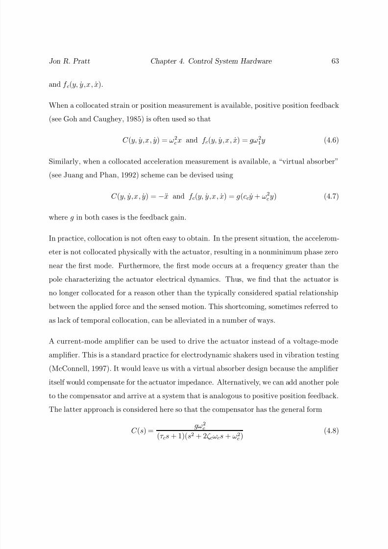
8/13/2019 Vibration Control for Chatter Suppression with Application to Boring Bars
http://slidepdf.com/reader/full/vibration-control-for-chatter-suppression-with-application-to-boring-bars 84/193

8/13/2019 Vibration Control for Chatter Suppression with Application to Boring Bars
http://slidepdf.com/reader/full/vibration-control-for-chatter-suppression-with-application-to-boring-bars 85/193
Jon R. Pratt Chapter 4. Control System Hardware 64
where g is the feedback gain, ωc and ζ c are the frequency and damping ratio associated
with the second-order dynamics of the compensator, and τ c is the time constant associated
with its first-order dynamics.
4.4.3 Compensator Design
We develop initially a compensator design strategy based on a single-degree-of-freedom
structural model with first-order actuator dynamics. The single-input, single-output plant
to be controlled is
G(s) = Ks2
(s2 + 2ζ 1ω1s + ω21)(s + α p)
(4.9)
where K = K 1K 2K sh1/L and α p = R/L.
Assuming positive feedback through the previously defined compensator C (s) yields the
characteristic equation
1 − G(s)C (s) = s6 + c5s5 + c4s4 + c3s3 + c2s2 + c1s + c0 = 0 (4.10)
where the coefficients cn are
c0 = ω21ω2
c α pαc
c1 = ω21ω2
c (α p + αc) + (2ζ 1ω1ω2c + 2ζ cωcω2
1)α pαc
c2 = ω21ω2
c + (2ζ 1ω1ω2c + 2ζ cωcω2
1)(α p + αc) + (ω21 + ω2
c + 4ζ 1ζ cω1ωc)α pαc − gKαcω2c
c3 = (2ζ 1ω1ω2c + 2ζ cωcω2
1) + (ω21 + ω2
c + 4ζ 1ζ cω1ωc)(α p + αc) + (2ζ 1ω1 + 2ζ cωc)α pαc
c4 = (ω21 + ω2
c + 4ζ 1ζ cω1ωc) + (2ζ 1ω1 + 2ζ cωc)(α p + αc) + α pαc
c5 = (2ζ 1ω1 + 2ζ cωc) + α p + αc
and αc = 1/τ . We seek a desired characteristic equation of the form
δ (s) = (s + β 1)(s + β 2)(s4 + p3s3 + p2s2 + p1s + p0) = 0 (4.11)

8/13/2019 Vibration Control for Chatter Suppression with Application to Boring Bars
http://slidepdf.com/reader/full/vibration-control-for-chatter-suppression-with-application-to-boring-bars 86/193
Jon R. Pratt Chapter 4. Control System Hardware 65
where β 1 and β 2 are arbitrary positive constants, and the coefficients pn are selected to
produce any desired complex poles. We choose to match the poles to an equivalent damped
vibration-absorber system and employ Den Hartog’s (1985) design criterion for the sake of
simplicity. Thus, the coefficients are determined by selecting a virtual mass ratio µ and
using the relations
p0 = ω4
1
(1 + µ)2, p1 =
2ω31ζ 2
(1 + µ),
p2 = ω21
2 + µ
1 + µ, p3 = 2ζ 2ω1, ζ 2 =
3µ
8(1 + µ)3
Knowing the pn, we equate the coefficients of Eqs. (4.10) and (4.11) and solve the resulting
set of six nonlinear algebraic equations for the unknown compensator values. The results
of this procedure using the parameters identified for the first mode of the system are shown
in Fig. 4.5 for the “effective” mass ratios µ = 0.1, 0.2, and 0.35. The resulting FRF’s
display the classic, “double hump” damped vibration-absorber structure.
Next, we examine the performance of a single-degree-of-freedom equivalent absorber-typecompensator design when the complete plant model (consisting of the four previously iden-
tified modes) is employed. We see in Fig. 4.6 that the “humps” of the response labeled
SDOF are no longer equal and that the performance is degraded. This mistuning can be
simply adjusted by reducing the feedback gain.
Consider the root locus of Fig. 4.7 where we focus on the behavior of the first structural
pole and that of the compensator. The root locus provides a map of the individual closed-
loop pole behaviors as a function of the feedback gain. Looking at the root locus, we might
choose to modify the design feedback gain such that the structural pole and compensator
pole migrate to points that lie along the same line radiating from the origin, so that the
poles have matched damping ratios. This design results in the curve labeled DAMP in Fig.
4.6. We see that the performance of such a design varies little from the SDOF equivalent

8/13/2019 Vibration Control for Chatter Suppression with Application to Boring Bars
http://slidepdf.com/reader/full/vibration-control-for-chatter-suppression-with-application-to-boring-bars 87/193
Jon R. Pratt Chapter 4. Control System Hardware 66
200.00 300.00 400.00 500.00 600.00 700.00
-40
-30
-20
-10
0
µ=0.1
µ=0.2
µ=0.35
Figure 4.5: Design results for various effective mass ratios.
absorber design. Another approach is to select the feedback gain such that the projections
of these poles along the real axis are equal. This design is labeled REAL in Fig. 4.6. We see
that this design has more of the classic absorber profile that we desire for chatter control.
The locations of the poles resulting from such a design are emphasized in the root locus
plot.
4.4.4 Structural Control Results
For our compensator, we use a 2nd-order analog circuit in conjunction with an off-the-
shelf, low-pass filter. The filter time constant is approximated by measuring the rate of
change of its phase angle with frequency; the result is τ = 0.0003175 seconds. This is a
crude approximation, even within the filter passband (0-2500 Hz), because it is actually a

8/13/2019 Vibration Control for Chatter Suppression with Application to Boring Bars
http://slidepdf.com/reader/full/vibration-control-for-chatter-suppression-with-application-to-boring-bars 88/193
Jon R. Pratt Chapter 4. Control System Hardware 67
200 300 400 500 600 700
-30
-20
-10
0
SDOF
DAMP
REAL
Figure 4.6: Closed-loop performance; single-degree-of-freedom design (SDOF), matched
damping design (DAMP), and matched projections along the real axis (REAL).

8/13/2019 Vibration Control for Chatter Suppression with Application to Boring Bars
http://slidepdf.com/reader/full/vibration-control-for-chatter-suppression-with-application-to-boring-bars 89/193
Jon R. Pratt Chapter 4. Control System Hardware 68
−1000 −900 −800 −700 −600 −500 −400 −300 −200 −100 00
500
1000
1500
2000
2500
3000
3500
4000
4500
5000
Real Axis
I m a g A x i s
Figure 4.7: Root locus of the system performance.
seven-pole elliptic filter; however, the accuracy is sufficient for purposes of illustration.
The assembled 2nd-order compensator has a natural frequency of 367 Hz, a damping ratio
of 0.707, and a static gain of 0.6ω2f . The design is not like those previously described but
was arrived at in an ad hoc fashion on the shop floor by trial and error. Nevertheless,
we plug the compensator values into our model and show a Bode plot of the predicted
closed-loop performance in Fig. 4.8. The actual performance is shown in Fig. 4.9.
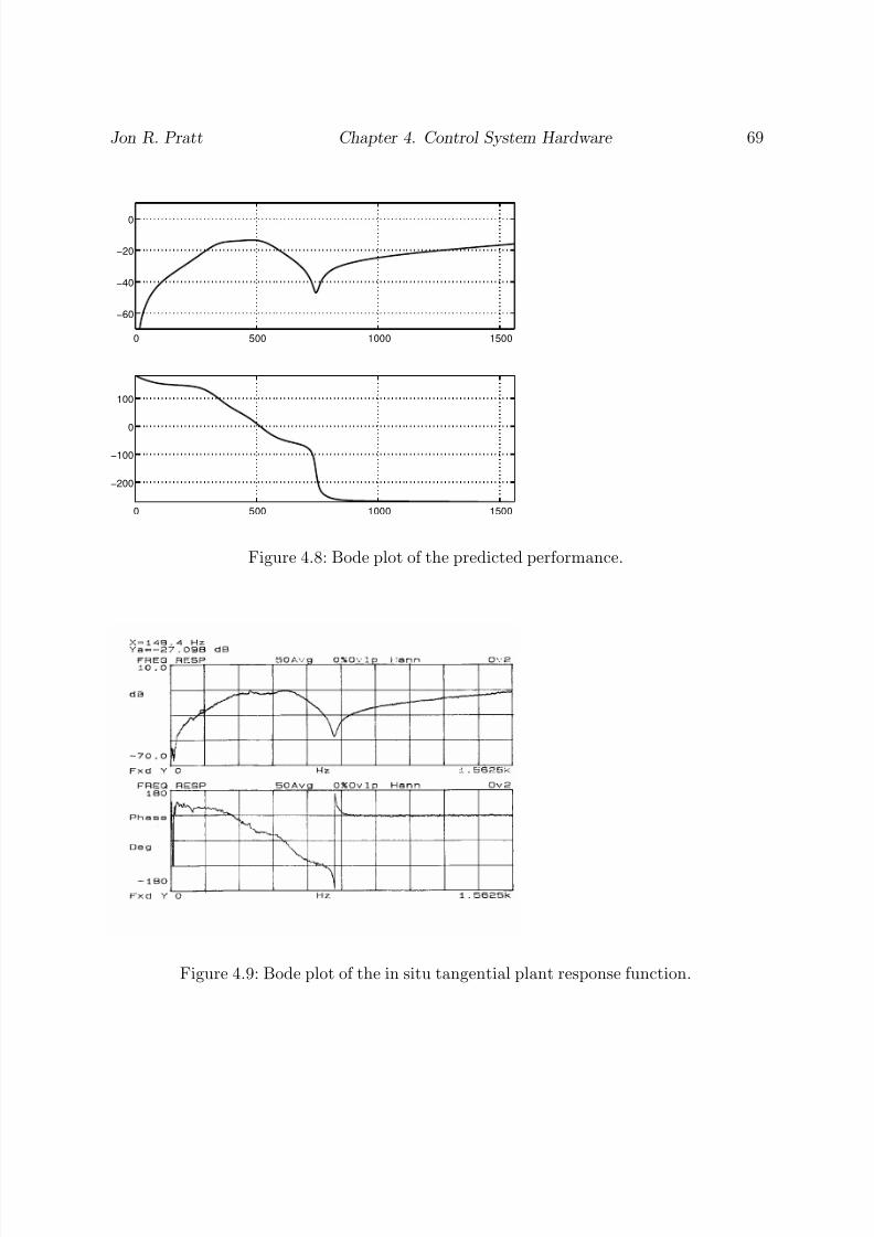
8/13/2019 Vibration Control for Chatter Suppression with Application to Boring Bars
http://slidepdf.com/reader/full/vibration-control-for-chatter-suppression-with-application-to-boring-bars 90/193
Jon R. Pratt Chapter 4. Control System Hardware 69
0 500 1000 1500
−60
−40
−20
0
0 500 1000 1500
−200
−100
0
100
Figure 4.8: Bode plot of the predicted performance.
Figure 4.9: Bode plot of the in situ tangential plant response function.
8/13/2019 Vibration Control for Chatter Suppression with Application to Boring Bars
http://slidepdf.com/reader/full/vibration-control-for-chatter-suppression-with-application-to-boring-bars 91/193
Part II
Nonlinear Machine-Tool Dynamics
and Control
70
8/13/2019 Vibration Control for Chatter Suppression with Application to Boring Bars
http://slidepdf.com/reader/full/vibration-control-for-chatter-suppression-with-application-to-boring-bars 92/193
Chapter 5
Chatter Observations and Smart Tool
Performance Testing
In this chapter, the Smart Tool of Chapter 4 is used to machine tubular aluminum spec-
imens. A variety of chatter signatures are recorded for cases with and without feedbackcontrol. Time traces, autospectra, cross spectra, and coherence are used to characterize the
tool motions during chatter conditions. We find evidence of coupling between the struc-
tural modes normal and tangential to the machined surfaces. Also, a jump phenomenon is
observed for a case without feedback control and also a case when control is applied only in
the direction tangent to the machined surface. A time trace of tool motions first without
feedback control and then with control demonstrates the ability of the smart machine-tool
system to suppress chatter.
71

8/13/2019 Vibration Control for Chatter Suppression with Application to Boring Bars
http://slidepdf.com/reader/full/vibration-control-for-chatter-suppression-with-application-to-boring-bars 93/193
Jon R. Pratt Chapter 5. Performance Testing 72
5.1 Description of Experiments
Tubular aluminum specimens of nominal inner diameter 4.5”-5.25”, outer diameter 6.1”,
and length 5” are machined to test the Smart Tool and to examine boring-bar chatter
dynamics. An example of a typical specimen is shown in the photo of Fig. 5.1.
Figure 5.1: Typical aluminum specimens,External File
A schematic of the measurment system is shown in Fig. 5.2. Acceleration time responses
normal and tangential to the machined surface are recorded using LabView software oper-
ating on a MacIntosh II data acquisition computer equipped with a National Instruments
NBMIO16x board. A Krohn Hite seven-pole elliptic low-pass filter with cutoff frequency of
2.5 kHz was used as an antialiasing filter. Unless otherwise stated, the data is sampled at
5 kHz for 10 seconds and subsequently broken into ten one-second duration ensembles that
are averaged in the frequency domain for the autospectra, cross spectrum, and coherence
plots. Post processing of the data is accomplished using routines written in MATLAB.
In some instances, spectral information is obtained using an HP 3562A two-channel signal
analyzer.
5.2 Results
The results reported here are from a variety of different test sessions conducted in the Man-
ufacturing Systems Laboratory of the Industrial Systems Engineering Department during
school holidays in August and December of 1996. Where appropriate, the nominal dynamic
properties of the Smart Tool are included in the description of individual results because
these properties varied due to differences in the assembly of the components from one test
period to the next.
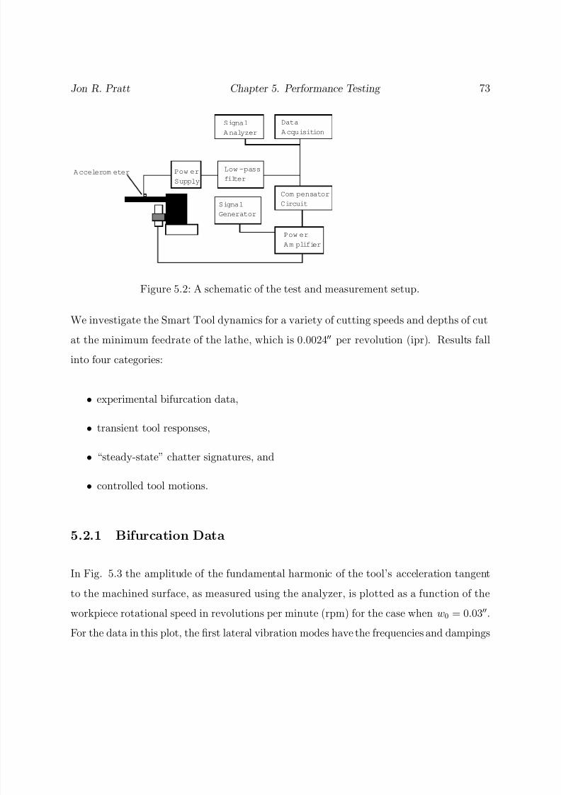
8/13/2019 Vibration Control for Chatter Suppression with Application to Boring Bars
http://slidepdf.com/reader/full/vibration-control-for-chatter-suppression-with-application-to-boring-bars 94/193
Jon R. Pratt Chapter 5. Performance Testing 73
Signal
Analyzer
Data
Acquisition
Pow er
Supply
Low -pass
filter
Pow er
Am plifier
Com pensator
CircuitSignal
Generator
Accelerom eter
Figure 5.2: A schematic of the test and measurement setup.
We investigate the Smart Tool dynamics for a variety of cutting speeds and depths of cut
at the minimum feedrate of the lathe, which is 0.0024 per revolution (ipr). Results fall
into four categories:
• experimental bifurcation data,
• transient tool responses,
• “steady-state” chatter signatures, and
• controlled tool motions.
5.2.1 Bifurcation Data
In Fig. 5.3 the amplitude of the fundamental harmonic of the tool’s acceleration tangent
to the machined surface, as measured using the analyzer, is plotted as a function of the
workpiece rotational speed in revolutions per minute (rpm) for the case when w0 = 0.03.
For the data in this plot, the first lateral vibration modes have the frequencies and dampings

8/13/2019 Vibration Control for Chatter Suppression with Application to Boring Bars
http://slidepdf.com/reader/full/vibration-control-for-chatter-suppression-with-application-to-boring-bars 95/193
Jon R. Pratt Chapter 5. Performance Testing 74
-1
4
9
14
50 90 130 170 210
g' s
250rpm
Figure 5.3: Bifurcation diagram showing the amplitude of the fundamental harmonic of
chatter for various spindle speeds when w = 0.03 and feedrate = 0.0024 ipr.
f t = 524 Hz and ζ t ≈ 0.03 and f n = 365 Hz and ζ n ≈ 0.02, respectively, as determined by
impact testing and circle fits of the resulting frequency-response functions.
Two observations can be made from the results in Fig. 5.3. First, the presence of sta-
ble cutting for all workpiece rotational speeds below 165 rpm indicates that the cutting
forces are dependent on the mean cutting velocity and contribute a positive damping at
low speeds, in agreement with Tlusty’s results (Tlusty, 1985) for aluminum. Second, a
subcritical-type instability occurs between 165 and 195 rpm, where both chatter and stable
cutting conditions coexist.

8/13/2019 Vibration Control for Chatter Suppression with Application to Boring Bars
http://slidepdf.com/reader/full/vibration-control-for-chatter-suppression-with-application-to-boring-bars 96/193
Jon R. Pratt Chapter 5. Performance Testing 75
5.2.2 Transient Data
Further evidence of subcritical-type instability is offered in the time record of Fig. 5.4,
where we record the progression from stable cutting to steady-state chatter in the tool
accelerations normal to the machined surface. The tool frequencies and dampings are
f t = 493 Hz and ζ t ≈ 0.03 and f n = 365 Hz and ζ n ≈ 0.02 and feedback control is inactive.
We see that, for the first five seconds of recorded data, the cut appears to be stable. After
approximately five seconds have elapsed, a hammer blow is administered to the tool in a
manner reminiscent of the experiments of Hooke and Tobias (1964). Clearly, chatter ensues,
though even after 80 seconds it has failed to reach a discernible steady state. The tool is
allowed to continue chattering in this fashion, and another data set is recorded after the
clearly audible (during the experiment) once per revolution variation in the tool vibrations
has subsided. This data is presented in Fig. 5.5 as an example of “steady-state” chattter
and will be more closely scrutinized in the following section on chatter signatures.
In Fig. 5.6 we consider the transient tool response to a hammer blow during stable cutting.
An exponentially decaying function is plotted along with the data to illustrate the relative
difference in damping between the motions in the normal and tangential directions for this
width and speed of cut. The exponential function is
a = aoe−ζω t (5.1)
where ao = 200, ζ = 0.15, and ω = 2π(365) for the normal direction, and ao = 35,
ζ = 0.028, and ω = 2π(524) for the tangential direction. Interestingly, the tool response
in the normal direction appears to be heavily damped by the cutting forces, while the tool
response in the direction tangent to the cut appears to be unaffected.

8/13/2019 Vibration Control for Chatter Suppression with Application to Boring Bars
http://slidepdf.com/reader/full/vibration-control-for-chatter-suppression-with-application-to-boring-bars 97/193
Jon R. Pratt Chapter 5. Performance Testing 76
0 5 10 15 20 25-100
0
100
a n
g s
30 35 40 45 50-100
0
100
a n
g s
55 60 65 70 75 80-100
0
100
a n
g s
Figure 5.4: Evolution of chatter in the tool response normal to the machined surface when
w = 0.002, speed = 90 rpm, and feedrate = 0.0024 ipr.
0 1 2 3 4 5-100
0
100
a n
g s
5.5 6 6.5 7 7.5 8 8.5 9 9.5 10 10.5-100
0
100
a n
g s
11 11.5 12 12.5 13 13.5 14 14.5 15 15.5-100
0
100
a n g
s
Figure 5.5: The time trace of the steady-state chatter normal to the machined surface when
w = 0.002, speed = 90 rpm, and feedrate = 0.0024 ipr.

8/13/2019 Vibration Control for Chatter Suppression with Application to Boring Bars
http://slidepdf.com/reader/full/vibration-control-for-chatter-suppression-with-application-to-boring-bars 98/193
Jon R. Pratt Chapter 5. Performance Testing 77
0 0.02 0.04 0.06 0.08 0.1-100
-50
0
50
100
a n
g s
0 0.02 0.04 0.06 0.08 0.1-20
-10
0
10
20
a t g s
Figure 5.6: The transient tool response to a hammer blow when w = 0.03, speed = 170
rpm, and feedrate = 0.0024 ipr.
5.2.3 Chatter Signatures
A great variety of chatter signatures were obtained in the two testing periods. Because the
tool dynamic properties were not identically the same in each period, we shall consider the
results separately.
Signatures from the test period of December, 1996.
We consider the time histories and autospectra of the tangential and normal accelerations
as well as the cross spectra and coherence between these signals for some typical chatter
signatures obtained when the tool frequencies and dampings are f t = 524 Hz and ζ t ≈ 0.03
and f n = 365 Hz and ζ n ≈ 0.02.
The tool dynamic properties during this set of tests are the same as those observed during
the bifurcation test, and we begin by contrasting two responses that were recorded during
8/13/2019 Vibration Control for Chatter Suppression with Application to Boring Bars
http://slidepdf.com/reader/full/vibration-control-for-chatter-suppression-with-application-to-boring-bars 99/193
Jon R. Pratt Chapter 5. Performance Testing 78
that experiment. The cutting conditions were maintained as nearly identical as possible
for both data records (same specimen, internal diameter, speed, feedrate, and depth of cut,
but at a different location along the tube). In Fig. 5.7 we see a typical spectral response for
a “stable” cutting condition. The tool response is a few tenths of a g in each direction and
the spectral content is indicative of a forced response due to “random” fluctuations in the
mean cutting force. Each spectrum shows evidence of the independent modal responses.
Comparing the tool response of Fig. 5.7 with the large chatter response of Fig. 5.8, we see
clearly that both stable and chattering motions coexist for the same cutting parameters.
In the chatter of Fig. 5.8 the spectral content is similar in each coordinate, with the tool
clearly undergoing a large-amplitude, harmonic mode coupled vibration.
Next, we see that it is possible to observe qualitatively different chatter signatures for the
same nominal cutting conditions. For instance, Fig. 5.9 shows large-amplitude chatter of
497 Hz that is dominated by tangential motions, while Fig. 5.10 shows large-amplitude
chatter of 416 Hz that is dominated by normal motions. These results are from the largest
width of cut w = 0.1 considered in the study. We note that the two experiments were not
precisely identical since the internal diameter of the specimen represented by the chatter
of Fig. 5.9 is 0.5 less than the specimen of Fig. 5.10.
Finally, the chatter signature of Fig. 5.11 is typical of tool responses obtained for shallow
cuts where the depth of cut is less than the nominal tool nose radius. These cuts are
dominated by tool motions normal to the machined surface.
Signatures from the test period of August, 1996.
Next, we consider the time histories and autospectra of the tangential and normal accelera-
tions as well as the cross spectra and coherence between these signals for chatter signatures
obtained when the tool frequencies and dampings are f t = 493 Hz and ζ t ≈ 0.03 and
f n = 365 Hz and ζ n ≈ 0.02. For this series of tests, the tool appeared far more prone to

8/13/2019 Vibration Control for Chatter Suppression with Application to Boring Bars
http://slidepdf.com/reader/full/vibration-control-for-chatter-suppression-with-application-to-boring-bars 100/193
Jon R. Pratt Chapter 5. Performance Testing 79
Figure 5.7: Stable tool response normal (bottom trace) and tangential (top trace) to the
machined surface when w = 0.03, speed = 190 rpm, and feedrate = 0.0024 ipr. Units are
g’s.
Figure 5.8: Chattering tool response normal (bottom trace) and tangential (top trace) to
the machined surface when w = 0.03, speed = 190 rpm, and feedrate = 0.0024 ipr. Units
are g’s.

8/13/2019 Vibration Control for Chatter Suppression with Application to Boring Bars
http://slidepdf.com/reader/full/vibration-control-for-chatter-suppression-with-application-to-boring-bars 101/193
Jon R. Pratt Chapter 5. Performance Testing 80
1 1.02 1.04-50
0
50
time (secs)
a n g
s
0 500 1000 1500 2000
-40
-200
20
freq (Hz)
d B s
497 Hz
1 1.02 1.04-50
0
50
time (secs)
a t g s
0 500 1000 1500 2000
-40
-20
0
20
freq (Hz)
d B s
497 Hz
0 500 1000 1500 2000
-40
-20
020
freq. (Hz)
d B s
0 500 1000 1500 20000
0.5
1
freq. (Hz)
c o h e r e n c
e
Figure 5.9: Tangentially oriented chatter signature when w = 0.1, speed = 235 rpm, and
feedrate = 0.0024 ipr.
chatter.
Chatter is observed at spindle rotational speeds as low as 90 rpm and for widths of cut as
small as 0.002, as seen in Fig. 5.12, which is the same data as the steady-state response
shown in Fig. 5.5. We note that for the shallow cut of 0.002, chatter tends to be localized
in a direction normal to the machined surface, whereas for the deeper cut of 0.03, chatter
is oriented more along a line tangent to the machined surface, as is evident in Fig. 5.13.
In both cases, the fundamental of the motion and its harmonics are seen to be linearly
coherent, suggesting that mode coupling is present.

8/13/2019 Vibration Control for Chatter Suppression with Application to Boring Bars
http://slidepdf.com/reader/full/vibration-control-for-chatter-suppression-with-application-to-boring-bars 102/193
Jon R. Pratt Chapter 5. Performance Testing 81
1 1.02 1.04
-10
0
10
time (secs)
a n g s
0 500 1000 1500 2000
-40
-200
20
freq (Hz)
d B s
416 Hz
1 1.02 1.04
-10
0
10
time (secs)
a t g s
0 500 1000 1500 2000
-40
-20
0
20
freq (Hz)
d B s
416 Hz
0 500 1000 1500 2000
-40
-20
020
freq. (Hz)
d B s
0 500 1000 1500 20000
0.5
1
freq. (Hz)
c o h e r e n c
e
Figure 5.10: Normally oriented chatter signature when w = 0.1, speed = 235 rpm, and
feedrate = 0.0024 ipr.
Figure 5.11: Chatter signature normal (bottom trace) and tangential (top trace) to the
machined surface when w = 0.005, speed = 195 rpm, and feedrate = 0.0024 ipr. Units are
g’s.

8/13/2019 Vibration Control for Chatter Suppression with Application to Boring Bars
http://slidepdf.com/reader/full/vibration-control-for-chatter-suppression-with-application-to-boring-bars 103/193
Jon R. Pratt Chapter 5. Performance Testing 82
1 1.02 1.04-10
0
10
time (secs)
a n g
s
(a)
0 500 1000 1500 2000-40
-20
0
freq (Hz)
a n
d B
s
424 Hz (b)
1 1.02 1.04-10
0
10
time (secs)
a t g s
(c)
0 500 1000 1500 2000
-40
-20
0
freq (Hz)
a t d B s
424 Hz (d)
0 500 1000 1500 2000-80
-60
-40-20
freq. (Hz)
c r o s s - s p e
c(e)
0 500 1000 1500 20000
0.5
1
freq. (Hz)
c o h e r e n c
e
(f)
Figure 5.12: Time traces, autospectra, cross-spectrum, and coherence when w = 0.002,
speed = 90 rpm, and feedrate = 0.0024 ipr.
5.2.4 Controlled Responses
Control performance was evaluated both in August and December of 1996 with similar
results. The data reported here is from August, and the dynamic properties of the structure
are those previously cited for that time period.
In Fig. 5.14, we show an example of a jump-type phenomenon in the time record of the
accelerations normal to the machined surface when only the tangential control loop is ac-
tive. Initially, the control is only active in the tangential direction. The cut appears to be
stable. A disturbance is introduced by hitting the bar in the normal direction with a ham-
mer. Clearly, the disturbance grows due to regeneration. After the chatter reaches steady
state, control is added in the normal direction, thereby stabilizing the system. Another
disturbance is applied but the control maintains stability. In Fig. 5.15, we show the time

8/13/2019 Vibration Control for Chatter Suppression with Application to Boring Bars
http://slidepdf.com/reader/full/vibration-control-for-chatter-suppression-with-application-to-boring-bars 104/193
Jon R. Pratt Chapter 5. Performance Testing 83
1 1.02 1.04-100
0
100
time (sec)
a n g
s
(a)
0 500 1000 1500 2000
-20
0
20
freq (Hz)
a n d B
s
473 Hz (b)
1 1.02 1.04-100
0
100
time (secs)
a t g s
(c)
0 500 1000 1500 2000
-20
0
20
40
freq (Hz)
a t d B s
473 Hz (d)
0 500 1000 1500 2000-20
0
2040
freq. (Hz)
c r o s s - s p
e c
(e)
0 500 1000 1500 20000
0.5
1
freq. (Hz)
c o h e r e n c e
(f)
Figure 5.13: Time traces, autospectra, cross-spectra, and coherence when w = 0.03, speed
= 210 rpm, and feedrate 0.0024 ipr.
traces, autospectra, cross-spectrum, and coherence of the normal and tangential accelera-
tions during steady-state chatter of this type. We see that though chatter is predominantly
oriented in the normal direction, a substantial tangential component exists.
Finally, we demonstrate biaxial control in Fig. 5.16. Large-amplitude chatter is allowed to
develop before applying feedback control in both directions that stabilizes the system. We
observe a dramatic improvement in the surface finish, as shown in the photo of Fig. 5.17.
5.3 Summary
In this chapter we have explored the dynamics of boring by observing the Smart Tool’s
behavior in a wide range of machining conditions. Transient responses, bifurcation experi-

8/13/2019 Vibration Control for Chatter Suppression with Application to Boring Bars
http://slidepdf.com/reader/full/vibration-control-for-chatter-suppression-with-application-to-boring-bars 105/193
Jon R. Pratt Chapter 5. Performance Testing 84
2 3 4 5 6 7 8 9 10 11 12-20
0
20Hammer Impact
14 15 16 17 18 19 20 21 22 23 24-20
0
20Control Applied
24 25 26 27 28 29 30 31 32 33 34-20
0
20
Hammer Impact
Figure 5.14: Time traces of the tool accelerations normal to the machined surface; initially,
only tangential control is active; then, in addition, control is applied in the normal direction
to quench the chatter and eliminate the jump-type instability; w = 0.002, speed = 170
rpm, and feedrate = 0.0024 ipr.
ments, and various chatter signatures provide evidence of a subcritical-type instability.
In general, we observe that shallow cuts, where the primary cutting edge is the tool nose
radius, give rise to chatter that is characterized by motions normal to the machined surface.
Deeper cuts that use more of the tool insert give rise to chatter that is characterized by
motions tangential to the machined surface. This behavior is most clear in the testing
period of August, 1996, where distinctions between the widths of cut w = 0.002 versus
w = 0.03 were consistent and obvious.
The distinction is less clear in the data obtained in the second testing period. Both tan-
gentially and normally oriented modes of chatter are witnessed in the very wide cuts of
Figs. 5.9 and 5.10. In Fig. 5.18 we see results for the intermediate width of cut w = 0.01
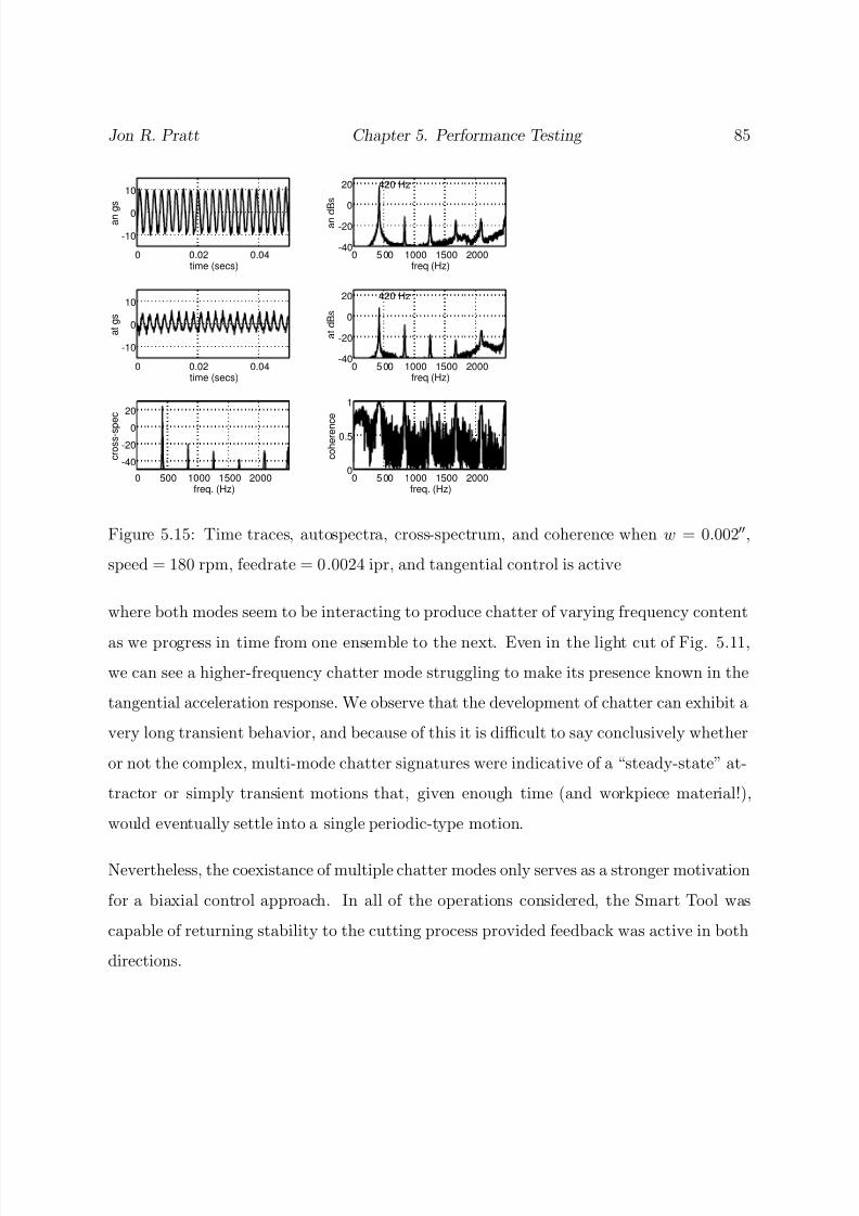
8/13/2019 Vibration Control for Chatter Suppression with Application to Boring Bars
http://slidepdf.com/reader/full/vibration-control-for-chatter-suppression-with-application-to-boring-bars 106/193
Jon R. Pratt Chapter 5. Performance Testing 85
0 0.02 0.04
-10
0
10
time (secs)
a n
g s
0 500 1000 1500 2000-40
-20
0
20
freq (Hz)
a n d
B s
420 Hz
0 0.02 0.04
-10
0
10
time (secs)
a t g s
0 500 1000 1500 2000-40
-20
0
20
freq (Hz)
a t d B s
420 Hz
0 500 1000 1500 2000
-40
-20
0
20
freq. (Hz)
c r o s s - s p
e c
0 500 1000 1500 20000
0.5
1
freq. (Hz)
c o h e r e n
c e
Figure 5.15: Time traces, autospectra, cross-spectrum, and coherence when w = 0.002,
speed = 180 rpm, feedrate = 0.0024 ipr, and tangential control is active
where both modes seem to be interacting to produce chatter of varying frequency content
as we progress in time from one ensemble to the next. Even in the light cut of Fig. 5.11,
we can see a higher-frequency chatter mode struggling to make its presence known in the
tangential acceleration response. We observe that the development of chatter can exhibit a
very long transient behavior, and because of this it is difficult to say conclusively whether
or not the complex, multi-mode chatter signatures were indicative of a “steady-state” at-
tractor or simply transient motions that, given enough time (and workpiece material!),
would eventually settle into a single periodic-type motion.
Nevertheless, the coexistance of multiple chatter modes only serves as a stronger motivation
for a biaxial control approach. In all of the operations considered, the Smart Tool was
capable of returning stability to the cutting process provided feedback was active in both
directions.
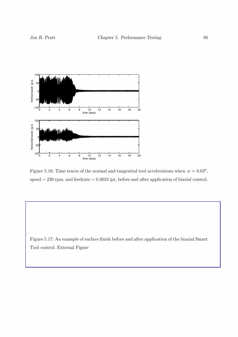
8/13/2019 Vibration Control for Chatter Suppression with Application to Boring Bars
http://slidepdf.com/reader/full/vibration-control-for-chatter-suppression-with-application-to-boring-bars 107/193
Jon R. Pratt Chapter 5. Performance Testing 86
0 2 4 6 8 10 12 14 16 18 20-100
-50
0
50
100
time (secs)
V e r t i c a l a c c e l . ( g
s )
0 2 4 6 8 10 12 14 16 18 20-100
-50
0
50
100
time (secs)
H o r i z o n t a l a c c e l . ( g
s )
Figure 5.16: Time traces of the normal and tangential tool accelerations when w = 0.03,
speed = 230 rpm, and feedrate = 0.0024 ipr, before and after application of biaxial control.
Figure 5.17: An example of surface finish before and after application of the biaxial Smart
Tool control. External Figure

8/13/2019 Vibration Control for Chatter Suppression with Application to Boring Bars
http://slidepdf.com/reader/full/vibration-control-for-chatter-suppression-with-application-to-boring-bars 108/193
Jon R. Pratt Chapter 5. Performance Testing 87
0
50
100
150
200
0
2
4
68
100
1
2
3
4
5
6
freq - 350 Hzensemble
a t g s
Figure 5.18: Waterfall plot of autospectra obtained from ten consecutive ensembles.
8/13/2019 Vibration Control for Chatter Suppression with Application to Boring Bars
http://slidepdf.com/reader/full/vibration-control-for-chatter-suppression-with-application-to-boring-bars 109/193
8/13/2019 Vibration Control for Chatter Suppression with Application to Boring Bars
http://slidepdf.com/reader/full/vibration-control-for-chatter-suppression-with-application-to-boring-bars 110/193
Jon R. Pratt Chapter 6. Nonlinear Dynamics 89
instability, the inadequacy of a two-term approximation, and the stability-limit of periodic
solutions. Having exhausted our purely analytical tools, we then explore the route to chaos
using computer simulation.
The material to this point is from Nayfeh, Chin, and Pratt (1997). The author gratefully
acknowledges the work of his coauthors, who performed the original bifurcation analysis,
and particularly the contributions of Dr. Char-Ming Chin, who produced the figures used
in this portion of the chapter.
In Section 6.4 we develop an analog-computer simulation to verify our analytical techniques.
We first confirm in Section 6.4.2 the global subcritical instability that was predicted via
harmonic-balance solutions and numerical integration. We revisit the route to chaos in
Section 6.4.2. We close Section 6.4 by considering the pointwise dimension of the experi-
mentally measured attractor using a reconstructed phase space. Finally, in Section 6.5 we
consider the effect of an absorber on the nonlinear stability of the model of Hanna and
Tobias (1974).
6.1 Normal Form of the Hopf Bifurcation
The equation of motion for the model of Hanna and Tobias (1974) was introduced in
Chapter 2 and is repeated here for convenience:
x + 2ξ x + p2(x + β 2x2 + β 3x3) = − p2w[x− xτ + α2(x − xτ )2 + α3(x− xτ )
3] (6.1)
where the paramaters as determined experimentally by Hanna and Tobias (1974) are p =
1088.56 rad/sec, ξ = 24792/ω rad2, β 2 = 479.3 1/in, β 3 = 264500 1/in2, α2 = 5.668 1/in,
and α3 = −3715.2 1/in2.
The nonlinearities considered in Eq. (6.1) include the nonlinear stiffness of the machine tool

8/13/2019 Vibration Control for Chatter Suppression with Application to Boring Bars
http://slidepdf.com/reader/full/vibration-control-for-chatter-suppression-with-application-to-boring-bars 111/193
Jon R. Pratt Chapter 6. Nonlinear Dynamics 90
and the nonlinear cutting force generated in the cutting process. According to the linear
analysis, a Hopf bifurcation occurs, leading to the birth of a limit cycle as w increases
past wc. The qualitative behavior in the neighborhood of this bifurcation point can be
predicted by studying the corresponding normal form. Due to the presence of both cubic
and quadratic nonlinearities, the perturbation analysis must be performed using either the
method of multiple scales or the generalized method of averaging (Nayfeh, 1973, 1981). In
this Dissertation, we choose a multiple-scales approach.
Using the method of multiple scales (Nayfeh, 1973, 1981), we introduce a fast time scale
T 0 = t and a slow time scale T 2 = 2t and seek a third-order expansion in the form
x = x1(T 0, T 2) + 2x2(T 0, T 2) + 3x3(T 0, T 2) + · · · (6.2)
Moreover, we let
w = wc + 2w2 + · · · (6.3)
Substituting Eqs. (6.2) and (6.3) into Eq. (6.1) and equating coefficients of like powers of
, we obtain
Order :
D20x1 + 2ξD0x1 + p2x1 + p2wc(x1 − x1τ ) = 0 (6.4)
Order 2:
D20x2 + 2ξD0x2 + p2x2 + p2wc(x2 − x2τ ) = − p2β 2x2
1 − p2wcα2(x1 − x1τ )2 (6.5)
Order 3:
D20x3 + 2ξD0x3 + p2x3 + p2wc(x3 − x3τ ) = −2D0D2x1 − 2ξD2x1 − p2w2(x1 − x1τ )
−2 p2β 2x1x2 − 2 p2wcα2(x1 − x1τ )(x2 − x2τ )
− p2β 3x31 − p2wcα3(x1 − x1τ )
3 (6.6)
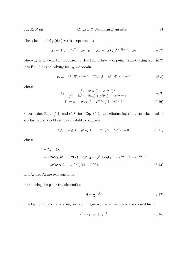
8/13/2019 Vibration Control for Chatter Suppression with Application to Boring Bars
http://slidepdf.com/reader/full/vibration-control-for-chatter-suppression-with-application-to-boring-bars 112/193
Jon R. Pratt Chapter 6. Nonlinear Dynamics 91
The solution of Eq. (6.4) can be expressed as
x1 = A(T 2)eiωcT 0 + cc, and x1τ = A(T 2)eiωc(T 0−τ ) + cc (6.7)
where ωc is the chatter frequency at the Hopf bifurcation point. Substituting Eq. (6.7)
into Eq. (6.5) and solving for x2, we obtain
x2 = − p2A2Γ1e2iωcT 0 − 2Γ2A A− p2 A2Γ1e−2iωcT 0 (6.8)
where
Γ1 = β
2 + w
cα2(1 − e−iωcτ )2
p2 − 4ω2c + 4iωcξ + p2wc(1 − e−2iωcτ ) (6.9)
Γ2 = β 2 + wcα2(1 − e−iωcτ )(1 − eiωcτ ) (6.10)
Substituting Eqs. (6.7) and (6.8) into Eq. (6.6) and eliminating the terms that lead to
secular terms, we obtain the solvability condition
2(ξ + iωc)A + p2w2(1− e−iωcτ )A + ΛA2 A = 0 (6.11)
where
Λ = Λr + iΛi
=−2 p2β 2( p2Γ1 + 2Γ2) + 3 p2β 3 − 2 p4wcα2Γ1(1 − eiωcτ )(1− e−2iωcτ )
+3 p2wcα3(1 − e−iωcτ )2(1 − eiωcτ ), (6.12)
and Λr and Λi are real constants.
Introducing the polar transformation
A = 1
2aeiβ (6.13)
into Eq. (6.11) and separating real and imaginary parts, we obtain the normal form
a = c1w2a + c2a3 (6.14)
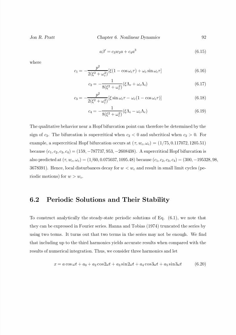
8/13/2019 Vibration Control for Chatter Suppression with Application to Boring Bars
http://slidepdf.com/reader/full/vibration-control-for-chatter-suppression-with-application-to-boring-bars 113/193
Jon R. Pratt Chapter 6. Nonlinear Dynamics 92
aβ = c3w2a + c4a3 (6.15)
where
c1 = − p2
2(ξ 2 + ω2c )
[ξ (1 − cos ωcτ ) + ωc sin ωcτ ] (6.16)
c2 = − 1
8(ξ 2 + ω2c )
(ξ Λr + ωcΛi) (6.17)
c3 = − p2
2(ξ 2 + ω2c )
[ξ sin ωcτ − ωc(1− cos ωcτ )] (6.18)
c4 = − 1
8(ξ 2 + ω2
c
)(ξ Λi − ωcΛr) (6.19)
The qualitative behavior near a Hopf bifurcation point can therefore be determined by the
sign of c2. The bifurcation is supercritical when c2 < 0 and subcritical when c2 > 0. For
example, a supercritical Hopf bifurcation occurs at (τ, wc, ωc) = (1/75, 0.117072, 1205.51)
because (c1, c2, c3, c4) = (159,−787737, 953,−2608438). A supercritical Hopf bifurcation is
also predicted at (τ, wc, ωc) = (1/60, 0.075037, 1095.48) because (c1, c2, c3, c4) = (300,−195328, 98,
3678391). Hence, local disturbances decay for w < wc and result in small limit cycles (pe-
riodic motions) for w > wc.
6.2 Periodic Solutions and Their Stability
To construct analytically the steady-state periodic solutions of Eq. (6.1), we note that
they can be expressed in Fourier series. Hanna and Tobias (1974) truncated the series by
using two terms. It turns out that two terms in the series may not be enough. We findthat including up to the third harmonics yields accurate results when compared with the
results of numerical integration. Thus, we consider three harmonics and let
x = a cos ωt + a0 + a2 cos2ωt + a3 sin2ωt + a4 cos3ωt + a5 sin3ωt (6.20)

8/13/2019 Vibration Control for Chatter Suppression with Application to Boring Bars
http://slidepdf.com/reader/full/vibration-control-for-chatter-suppression-with-application-to-boring-bars 114/193
Jon R. Pratt Chapter 6. Nonlinear Dynamics 93
Substituting Eq. (6.20) into Eq. (6.1) and equating the coefficient of each harmonic on both
sides, we obtain a system of seven nonlinear algebraic equations. The algebra was carried
out by using a symbolic manipulator. We numerically calculate the roots of this system of
equations and hence ω and the ai. Due to the lengthy expressions in these equations, we
only show the numerical results in the figures.
To determine the stability of a periodic solution x0(t), we use Floquet theory (Nayfeh
and Mook, 1979; Nayfeh and Balachandran, 1995). We first perturb the periodic solution
x = x0(t) by introducing a disturbance term u(t) and obtain
x(t) = x0(t) + u(t) (6.21)
Substituting Eq.(6.21) into Eq. (6.1) and linearizing in the disturbance u, we obtain
u+2ξ u + p2(1+2β 2x0 +3β 3x20)u = − p2w[1+2α2(x0−x0τ )+3α3(x0−x0τ )
2](u−uτ ) (6.22)
According to Floquet theory, Eq. (6.22) admits solutions of the form
u(t) = eγtφ(t) (6.23)
where φ(t) is a periodic function with period T = 2π/ω, which is equal to the period of
x0(t). Substituting Eq. (6.23) into Eq. (6.22) yields
φ + 2γ φ + γ 2φ+ 2ξγφ + 2ξ φ + p2(1 + 2β 2x0 + 3β 3x20)φ
=− p2w[1 + 2α2(x0 − x0τ ) + 3α3(x0 − x0τ )2](φ− e−γτ φτ ) (6.24)
To solve Eq. (6.24), we expand φ in a Fourier series and keep up to the third harmonics
for consistency with Eq. (6.20). Thus, we let
φ = b1 cos ωt + b2 sin ωt + b0 + b3 cos2ωt + b4 sin2ωt + b5 cos3ωt + b6 sin3ωt (6.25)
Substituting Eq. (6.25) into Eq. (6.24) and equating the coefficient of each harmonic on
both sides, we obtain a system of seven linear homogeneous algebraic equations governing

8/13/2019 Vibration Control for Chatter Suppression with Application to Boring Bars
http://slidepdf.com/reader/full/vibration-control-for-chatter-suppression-with-application-to-boring-bars 115/193
Jon R. Pratt Chapter 6. Nonlinear Dynamics 94
the bm. Setting the determinant of the coefficient matrix of this system equal to zero, we
obtain the so-called Hill’s determinant governing γ . This determinant is more complex
than a common polynomial form due to the time delay τ . Again, the algebra was carried
out by using a symbolic manipulator.
It follows from Eq. (6.23) that a given periodic solution x0(t) is asymptotically stable if
and only if all of the eigenvalues γ lie in the left-half plane and it is unstable if at least one
eigenvalue lies in the right-half plane. Starting with a width of cut w for which periodic
solutions are stable and then increasing w, we find that these periodic solutions will undergo
a bifurcation and hence lose stability. The response subsequent to the bifurcation depends
on the manner in which the eigenvalues move from the left- to the right-half plane. If a
real eigenvalue moves from the left- to the right-half plane along the real axis, the system
response will jump to another solution, which in this case may be periodic or trivial. On
the other hand, when a pair of complex conjugate eigenvalues moves transversely from the
left- to the right-half plane, the resulting response will be either a two-period quasiperiodic
motion or a periodic motion with a large period (phase-locked motion).
6.3 Numerical Results
As a first step, we validate the analytical results by numerically integrating Eq. (6.1). For
the numerical integration, we use a fifth-order Runge-Kutta scheme. Then, we start with
some initial conditions and, as in the actual cutting process, let xτ = 0 for 0 ≤ t < τ
and switch on xτ for t ≥ τ. The integration is carried out long enough for the transients
to die out. The numerically obtained periodic solutions are very close to those obtained
analytically so much so that they are indistinguishable when plotted together. Therefore,
we show in Fig. 6.1 two-dimensional projections of the phase portraits of the periodic
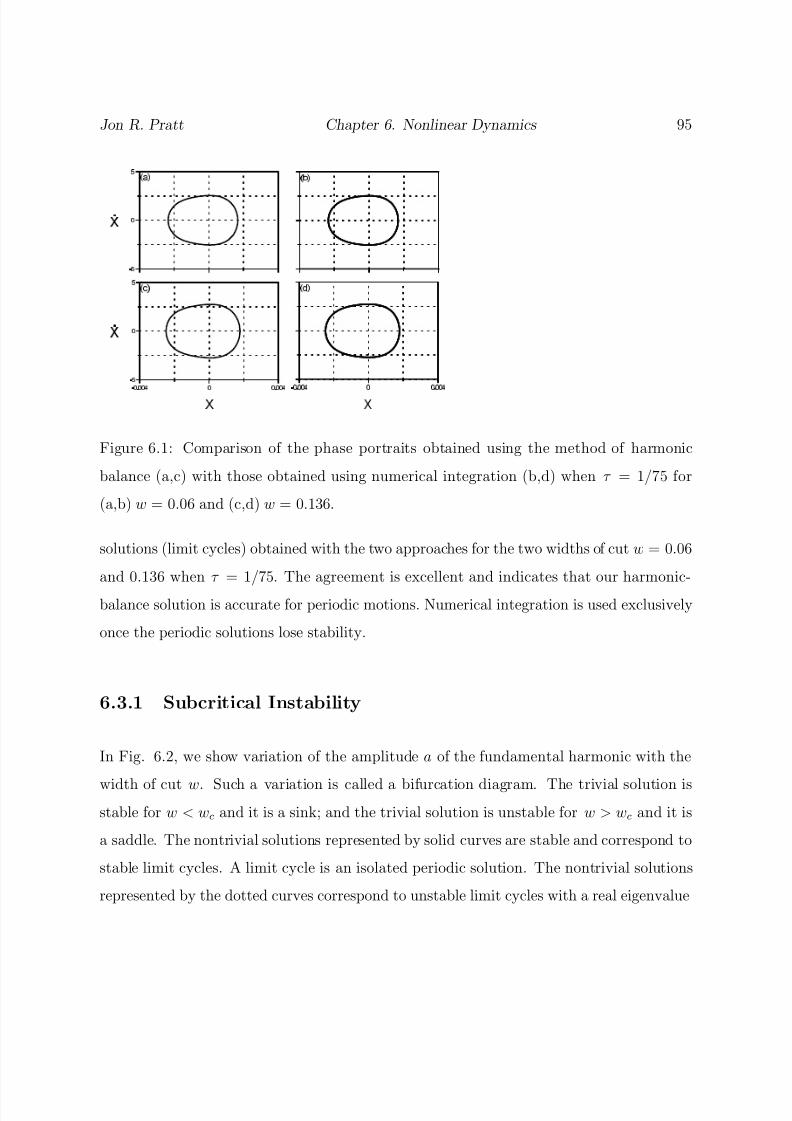
8/13/2019 Vibration Control for Chatter Suppression with Application to Boring Bars
http://slidepdf.com/reader/full/vibration-control-for-chatter-suppression-with-application-to-boring-bars 116/193
Jon R. Pratt Chapter 6. Nonlinear Dynamics 95
Figure 6.1: Comparison of the phase portraits obtained using the method of harmonic
balance (a,c) with those obtained using numerical integration (b,d) when τ = 1/75 for
(a,b) w = 0.06 and (c,d) w = 0.136.
solutions (limit cycles) obtained with the two approaches for the two widths of cut w = 0.06
and 0.136 when τ = 1/75. The agreement is excellent and indicates that our harmonic-
balance solution is accurate for periodic motions. Numerical integration is used exclusively
once the periodic solutions lose stability.
6.3.1 Subcritical Instability
In Fig. 6.2, we show variation of the amplitude a of the fundamental harmonic with the
width of cut w. Such a variation is called a bifurcation diagram. The trivial solution is
stable for w < wc and it is a sink; and the trivial solution is unstable for w > wc and it is
a saddle. The nontrivial solutions represented by solid curves are stable and correspond to
stable limit cycles. A limit cycle is an isolated periodic solution. The nontrivial solutions
represented by the dotted curves correspond to unstable limit cycles with a real eigenvalue
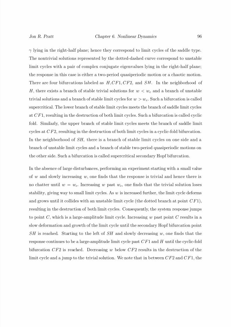
8/13/2019 Vibration Control for Chatter Suppression with Application to Boring Bars
http://slidepdf.com/reader/full/vibration-control-for-chatter-suppression-with-application-to-boring-bars 117/193
Jon R. Pratt Chapter 6. Nonlinear Dynamics 96
γ lying in the right-half plane; hence they correspond to limit cycles of the saddle type.
The nontrivial solutions represented by the dotted-dashed curve correspond to unstable
limit cycles with a pair of complex conjugate eigenvalues lying in the right-half plane;
the response in this case is either a two-period quasiperiodic motion or a chaotic motion.
There are four bifurcations labeled as H,CF 1, CF 2, and SH . In the neighborhood of
H , there exists a branch of stable trivial solutions for w < wc and a branch of unstable
trivial solutions and a branch of stable limit cycles for w > wc. Such a bifurcation is called
supercritical. The lower branch of stable limit cycles meets the branch of saddle limit cycles
at C F 1, resulting in the destruction of both limit cycles. Such a bifurcation is called cyclic
fold. Similarly, the upper branch of stable limit cycles meets the branch of saddle limit
cycles at C F 2, resulting in the destruction of both limit cycles in a cyclic-fold bifurcation.
In the neighborhood of SH, there is a branch of stable limit cycles on one side and a
branch of unstable limit cycles and a branch of stable two-period quasiperiodic motions on
the other side. Such a bifurcation is called supercritical secondary Hopf bifurcation.
In the absence of large disturbances, performing an experiment starting with a small value
of w and slowly increasing w, one finds that the response is trivial and hence there is
no chatter until w = wc. Increasing w past wc, one finds that the trivial solution loses
stability, giving way to small limit cycles. As w is increased further, the limit cycle deforms
and grows until it collides with an unstable limit cycle (the dotted branch at point C F 1),
resulting in the destruction of both limit cycles. Consequently, the system response jumps
to point C , which is a large-amplitude limit cycle. Increasing w past point C results in a
slow deformation and growth of the limit cycle until the secondary Hopf bifurcation point
SH is reached. Starting to the left of SH and slowly decreasing w, one finds that the
response continues to be a large-amplitude limit cycle past C F 1 and H until the cyclic-fold
bifurcation CF 2 is reached. Decreasing w below CF 2 results in the destruction of the
limit cycle and a jump to the trivial solution. We note that in between CF 2 and C F 1, the

8/13/2019 Vibration Control for Chatter Suppression with Application to Boring Bars
http://slidepdf.com/reader/full/vibration-control-for-chatter-suppression-with-application-to-boring-bars 118/193
Jon R. Pratt Chapter 6. Nonlinear Dynamics 97
system response may be trivial (no chatter) or a large-amplitude limit cycle (chatter with a
large amplitude), depending on the initial conditions. This phenomenon is usually referred
to as a subcritical instability. As a consequence, the nonlinearity reduces the instability
limit w = wc ≈ 0.117072 predicted by the linear theory, to w ≈ 0.0431, corresponding to
CF 2, a reduction of about 63%. The subcritical instability was observed experimentally
by Hanna and Tobias (1974).
In Fig. 6.3 for τ = 1/60, which is referred to as the left side of the lobe (see Fig. 2.8),
the small periodic solution born as a result of the supercritical Hopf bifurcation, instead of
quickly suffering a jump via a cyclic-fold bifurcation, grows smoothly and remains stable
as w increases until it undergoes a cyclic-fold bifurcation at w > 4.0. Another perspective
of this type of behavior is shown in Fig. 6.4 for w = 0.1. All of the Hopf bifurcations are
supercritical. As the rotational speed decreases, every Hopf bifurcation occurring at the
right end of an unstable branch of trivial solutions (or the right side of the shaded area
in Fig. 2.8) gives birth to a small periodic solution, which immediately suffers a cyclic-
fold bifurcation, resulting in a jump to an upper branch of stable periodic solutions. On
the other hand, every Hopf bifurcation occurring at the left end leads to a small periodic
solution whose amplitude grows smoothly with increasing rotational speed.
6.3.2 Inadequacy of the Two-Term Approximation
We compare in Fig. 6.2 the analytical results obtained with the two-term and six-term
approximations in the Fourier series when τ = 1/75. Except for the small-amplitude limit
cycles for values of w near wc, as shown in the inset, the two approximations yield results
that are very close. However, whereas the six-term approximation predicts a secondary
Hopf bifurcation at w ≈ 0.141, the two-term approximation predicts stable limit cycles.
When τ = 1/60, the results in Fig. 6.3 show that the two-term approximation predicts
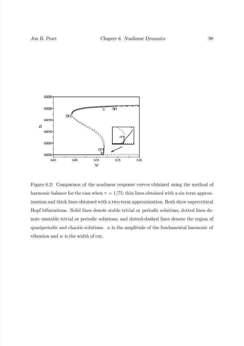
8/13/2019 Vibration Control for Chatter Suppression with Application to Boring Bars
http://slidepdf.com/reader/full/vibration-control-for-chatter-suppression-with-application-to-boring-bars 119/193
Jon R. Pratt Chapter 6. Nonlinear Dynamics 98
Figure 6.2: Comparison of the nonlinear response curves obtained using the method of
harmonic balance for the case when τ = 1/75: thin lines obtained with a six-term approx-
imation and thick lines obtained with a two-term approximation. Both show supercritical
Hopf bifurcations. Solid lines denote stable trivial or periodic solutions, dotted lines de-
note unstable trivial or periodic solutions, and dotted-dashed lines denote the region of
quasiperiodic and chaotic solutions. a is the amplitude of the fundamental harmonic of
vibration and w is the width of cut.

8/13/2019 Vibration Control for Chatter Suppression with Application to Boring Bars
http://slidepdf.com/reader/full/vibration-control-for-chatter-suppression-with-application-to-boring-bars 120/193
Jon R. Pratt Chapter 6. Nonlinear Dynamics 99
Figure 6.3: Comparison of the nonlinear response curves obtained using the method of
harmonic balance for the case when τ = 1/60: thin lines obtained with a six-term approxi-
mation and thick lines obtained with a two-term approximation. The two-term approxima-
tion erroneously predicts a subcritical rather than a supercritical Hopf bifurcation. Solid
lines denote stable trivial or periodic solutions and dotted lines denote unstable trivial or
periodic solutions. a is the amplitude of the fundamental harmonic of vibration and w is
the width of cut.

8/13/2019 Vibration Control for Chatter Suppression with Application to Boring Bars
http://slidepdf.com/reader/full/vibration-control-for-chatter-suppression-with-application-to-boring-bars 121/193
Jon R. Pratt Chapter 6. Nonlinear Dynamics 100
τ
Figure 6.4: Nonlinear response curves for a six-term approximation when w = 0.1. Solid
lines denote stable trivial or periodic solutions and dotted lines denote unstable trivial or
periodic solutions. a is the amplitude of the fundamental harmonic of vibration and w is
the width of cut.
8/13/2019 Vibration Control for Chatter Suppression with Application to Boring Bars
http://slidepdf.com/reader/full/vibration-control-for-chatter-suppression-with-application-to-boring-bars 122/193
Jon R. Pratt Chapter 6. Nonlinear Dynamics 101
qualitatively erroneous results; it predicts a subcritical rather than a supercritical Hopf
bifurcation, as shown in the inset.
Because of the unsymmetrical nature of the quadratic stiffness and cutting force, at least
the second-harmonic terms need to be included in the method of harmonic balance. As
shown in the previous section, the normal form, obtained by using the method of multiple
scales, qualitatively predicts accurate results because it accounts for the effects of both the
quadratic and cubic nonlinearities.
6.3.3 Route to Chaos
Next, we investigate the behavior of the motions for values of w exceeding that correspond-
ing to the secondary Hopf bifurcation SH by using a numerical integration of the governing
equation (6.1) for a time long enough for the transients to die out. To characterize the
motions, we use four tools, namely, phase portraits, time traces, Poincare sections, and
power spectra. For the Poincare sections, we collected all of the points of intersection of
the trajectory with the surface of section x(t − τ ) = 0 when x(t − τ ) > 0.
In Fig. 6.5, we show characteristics of the motion when w = 0.136. As expected, the motion
is periodic: the phase portrait is a closed curve, the Poincare section consists of a finite
number of points (one point), and the power spectrum consists of a fundamental frequency
and its even and odd harmonics, including a constant component (usually referred to as dc
component). The magnitudes of the peaks are in good agreement with those obtained by
using the method of harmonic balance.
As w increases, the limit cycle increases in size, deforms, and loses stability via a secondary
Hopf bifurcation SH with a pair of complex conjugate eigenvalues γ crossing transversely
from the left-half to the right-half plane. At w 0.141, a pair of the eigenvalues is
8/13/2019 Vibration Control for Chatter Suppression with Application to Boring Bars
http://slidepdf.com/reader/full/vibration-control-for-chatter-suppression-with-application-to-boring-bars 123/193
Jon R. Pratt Chapter 6. Nonlinear Dynamics 102
γ = 0.1166 ± 267.372i, the chatter frequency ω1 = 1391.07, and the bifurcated solution
can be characterized by two independent frequencies ω1 and ω2, which are, in general,
incommensurate (i.e., ω2/ω1, is not a rational number). Characteristics of this motion
are shown in Fig. 6.6. Such a motion is called two-period quasiperiodic or two-torus.
The time trace suggests that the motion contains two periods and the power spectrum
clearly contains another frequency besides the original chatter frequency. The ratio of
the chatter frequency ω1 = 1391.07 to the modulated frequency ω2 = 267.37 is 5.203
approximately. As indicated by the power spectrum, the two peaks on both sides of the
fundamental frequency component are about 0.4ω1 apart. The phase portrait seems not
to close on itself, suggesting a nonperiodic motion. The collected points on the one-sided
Poincare section fill up uniformly and densely a closed curve, confirming the two-period
quasiperiodic nature of the motion. Such a motion can be calculated by using a spectral
analysis. Keeping up to the second harmonics and sum and difference of the harmonics,
one can approximate such a motion with
x(t) = a0 + a1 cos ω1t + a2 cos2ω1t + a3 sin2ω1t + b1 cos ω2t + b2 cos2ω2t + b3 sin2ω2t
+c1 cos[(ω2 + ω1)t] + c2 sin[(ω2 + ω1)t] + c3 cos[(ω2 − ω1)t] + c4 sin[(ω2 − ω1)t]
Substituting Eq. (6.26) into Eq. (6.1) and equating the coefficient of each harmonic on
both sides, one obtains a system of 13 nonlinear algebraic equations for the ai, bi, ci, ω1, and
ω2. This we leave for future research, and the remaining results are obtained via numerical
integration.
As w is increased substantially above 0.141, the Poincare section gets distorted and the
collected points on the surface of section cover the closed curve nonuniformly, as shown
in Fig. 6.7 when w = 0.230. The power spectrum contains many more frequencies. As w
increases further, the torus grows and doubles, as shown in Fig. 6.8 for w = 0.240. The
post-bifurcation state is a new torus that forms two loops around the original torus. The
power spectrum of the doubled torus has many more frequencies than that of the torus
8/13/2019 Vibration Control for Chatter Suppression with Application to Boring Bars
http://slidepdf.com/reader/full/vibration-control-for-chatter-suppression-with-application-to-boring-bars 124/193
Jon R. Pratt Chapter 6. Nonlinear Dynamics 103
in Fig. 6.7. Instead of undergoing a complete cascade of period-doubling bifurcations,
the doubled torus deforms into a wrinkled one, followed by a fractal torus, and finally a
destruction of the torus and the emergence of a chaotic attractor, as shown in the Poincare
sections of Figs. 6.9 and 6.10. This transition to chaos through a two-period quasiperiodic
attractor is often described as chaos via torus breakdown (Nayfeh and Balachandran, 1995).
6.3.4 Influence of Nonlinear Stiffness
In this section, we ascertain the importance of the nonlinear stiffness terms β 2x2 and β 3x3
on the response of the machine tool. To this end, we compare in Fig. 6.11 the nonlinear
responses for the cases with nonlinear stiffness and those without nonlinear stiffness (β 2 =
β 3 = 0). Clearly the nonlinear stiffness terms have a profound influence on the system
behavior. Neglecting the nonlinear stiffness terms eliminates the cyclic-fold and hence
eliminates the subcritical instability.
6.4 Analog-Computer Simulation Results
In order to solve Eq. (6.1) on the analog computer, we first assume that the highest
derivative term is known and write the equation as follows:
x = −2ξ x − p2(x + β 2x2 + β 3x3) − p2w[x − xτ + α2(x − xτ )2 + α3(x − xτ )
3] (6.26)
We note, that the coefficients of Eq. (6.26) are poorly scaled for the analog computer. Tobegin, we let
x = u/β 2 (6.27)
in Eq. (6.26) and obtain
u = −2ξ u − p2(u + u2 + 1.15u3)
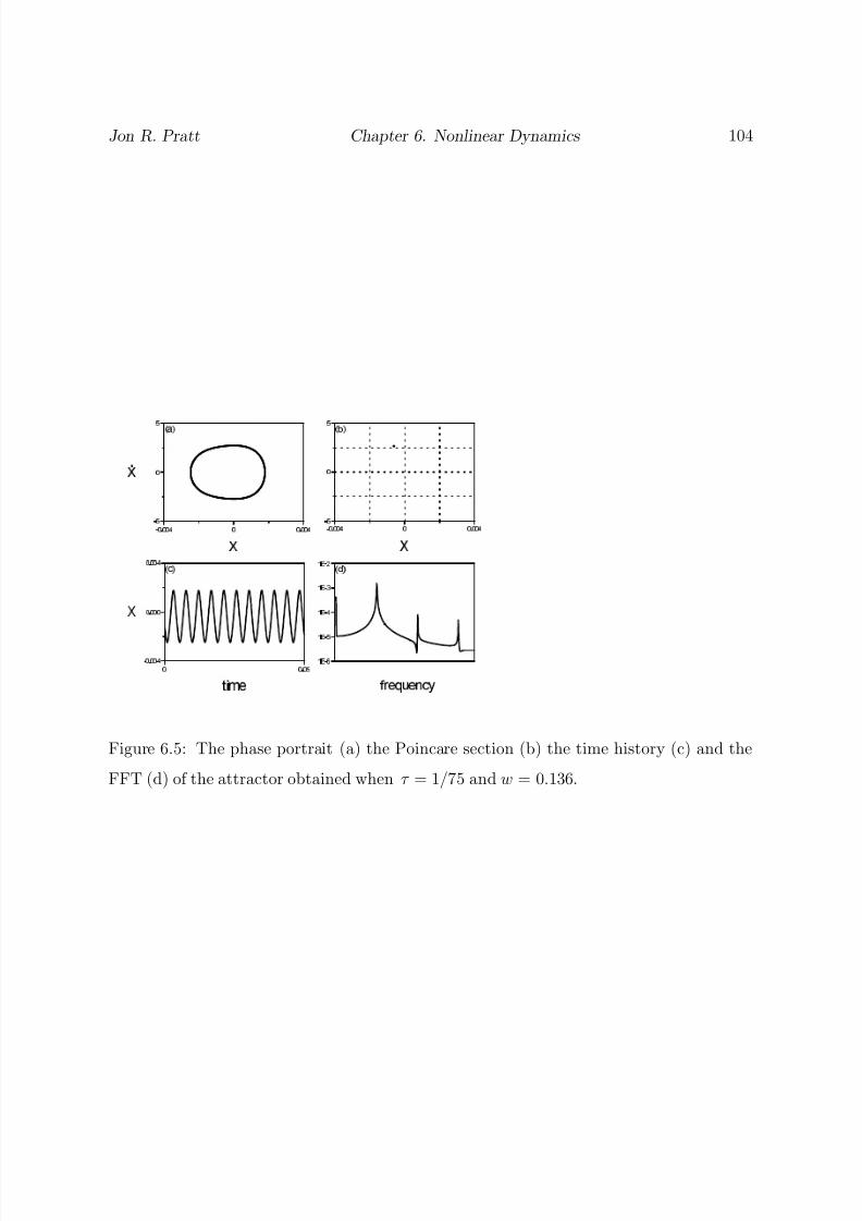
8/13/2019 Vibration Control for Chatter Suppression with Application to Boring Bars
http://slidepdf.com/reader/full/vibration-control-for-chatter-suppression-with-application-to-boring-bars 125/193
Jon R. Pratt Chapter 6. Nonlinear Dynamics 104
Figure 6.5: The phase portrait (a) the Poincare section (b) the time history (c) and the
FFT (d) of the attractor obtained when τ = 1/75 and w = 0.136.

8/13/2019 Vibration Control for Chatter Suppression with Application to Boring Bars
http://slidepdf.com/reader/full/vibration-control-for-chatter-suppression-with-application-to-boring-bars 126/193

8/13/2019 Vibration Control for Chatter Suppression with Application to Boring Bars
http://slidepdf.com/reader/full/vibration-control-for-chatter-suppression-with-application-to-boring-bars 127/193
Jon R. Pratt Chapter 6. Nonlinear Dynamics 106
Figure 6.8: The phase portrait (a) the Poincare section (b) the time history (c) and the
FFT (d) of the attractor obtained when τ = 1/75 and w = 0.240.
− p2w[u − uτ + .012(u − uτ )2 − .016(u − uτ )
3] (6.28)
Next, we rescale time to obtain a linear natural frequency of 10 rad/s and rewrite Eq.
(6.28) as
u =−.41886u − 100(u + u2 + 1.15u3)
−100[u − uτ + 0.012(u − uτ )2
−0.016(u − uτ )3] (6.29)
where the prime denotes the derivative with respect to
t = 108.856t (6.30)

8/13/2019 Vibration Control for Chatter Suppression with Application to Boring Bars
http://slidepdf.com/reader/full/vibration-control-for-chatter-suppression-with-application-to-boring-bars 128/193
Jon R. Pratt Chapter 6. Nonlinear Dynamics 107
Figure 6.9: The Poincare sections obtained when τ = 1/75 and w = (a) 0.250 (b) 0.255 (c)
0.260 (d) 0.265 (e) 0.266 and (f) 0.267.
Figure 6.10: The Poincare sections obtained when τ = 1/75 and w = (a) 0.270 (b) 0.30 (c)
0.32 and (d) 0.35.
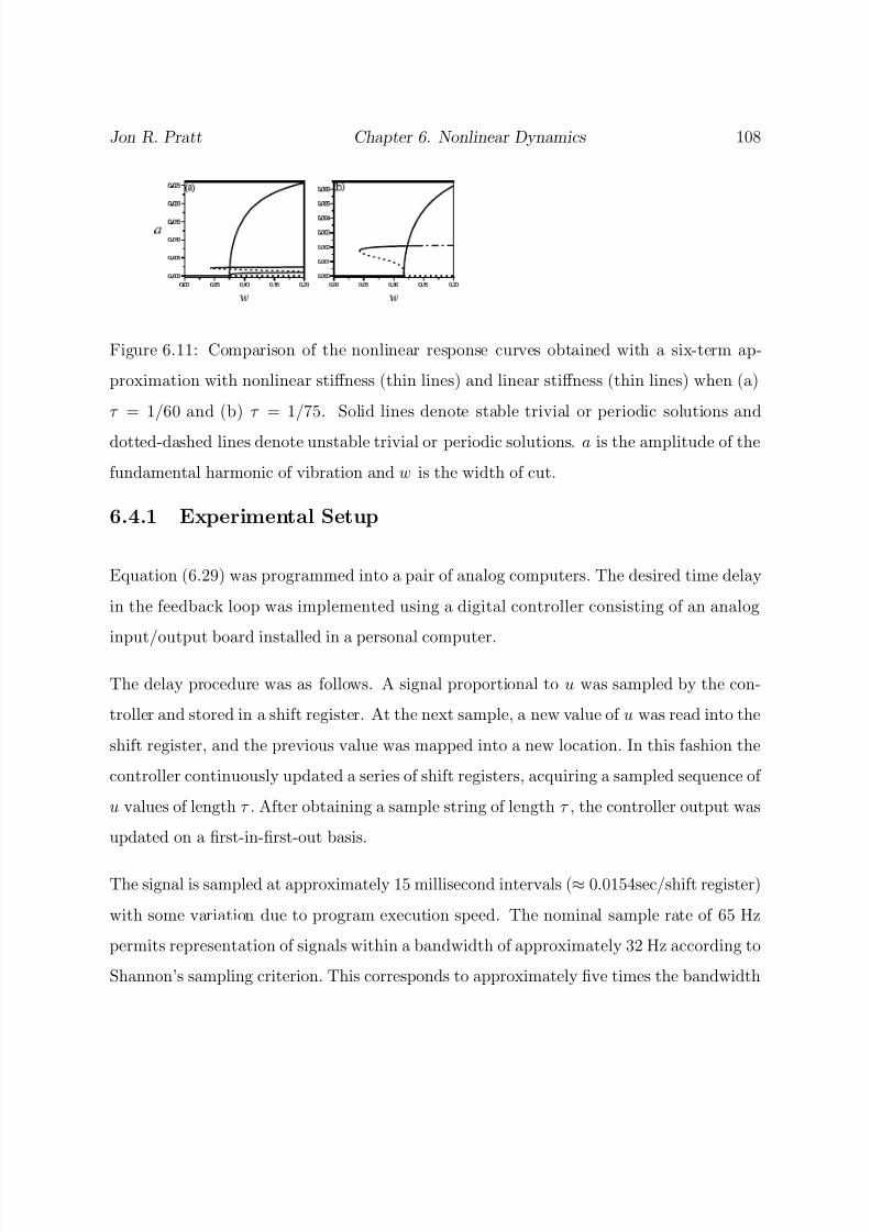
8/13/2019 Vibration Control for Chatter Suppression with Application to Boring Bars
http://slidepdf.com/reader/full/vibration-control-for-chatter-suppression-with-application-to-boring-bars 129/193

8/13/2019 Vibration Control for Chatter Suppression with Application to Boring Bars
http://slidepdf.com/reader/full/vibration-control-for-chatter-suppression-with-application-to-boring-bars 130/193
Jon R. Pratt Chapter 6. Nonlinear Dynamics 109
required to reproduce the fundamental and first two harmonics of the combined system
response. As such, the sampling interval seems small enough to approximate a continuous
time controller. However, in the author’s experience, there exists no reliable criterion as to
what constitutes “real” time discretization when the plant is nonlinear. As in numerical
integration, the time step is small enough when the results make sense.
To evaluate the timing of the digital delay, we tested the controller using a square wave
input from a signal generator. The input and output of the delay were captured using a
dual-channel, digital-storage oscilloscope, and the time lag between the signals then was
recorded. Ten measurements of the delay revealed that the actual experimental value of τ
varied approximately 0.5 percent around a mean value. This variation was attributed to
fluctuations in the program execution speed.
In the following sections, we present and discuss results obtained using the analog computer
to integrate Eq. (6.29). All integrations were carried out long enough for transients to
die out. Data were recorded using both a spectrum analyzer and a multichannel data
acquisition board. The specifics of the data-acquisition will be discussed where appropriate.
6.4.2 Bifurcation Diagrams
As a first step in the experimental analysis, we sought to reproduce the bifurcation diagrams
that were developed using the six-term harmonic balance. An experiment was performed
beginning with a small value of w and observing the system response to prescribed ini-
tial conditions. After the system reached steady state, a spectrum analyzer was used to
compute the average power spectrum of u using a Hanning window and 5 averages. The
amplitude a of the fundamental frequency component was recorded in units of peak Volts
and then scaled accordingly. The frequency resolution was 0.012 Hz and a typical funda-
8/13/2019 Vibration Control for Chatter Suppression with Application to Boring Bars
http://slidepdf.com/reader/full/vibration-control-for-chatter-suppression-with-application-to-boring-bars 131/193
Jon R. Pratt Chapter 6. Nonlinear Dynamics 110
mental frequency was approximately 2.0 Hz (analog-computer time scale). We note that in
hindsight, a flattop window would have been more appropriate for precise measurement of
the amplitudes. The frequency of the measured periodic motions was a continuously vary-
ing function of the control parameter, and, in the course of generating the bifurcation set,
measurements were made of periodic responses that had frequencies between the available
spectral lines. This problem of spectral resolution explains some of the data fluctuation
that will be observed.
In the bifurcation diagram of Fig. 6.12 (a), we compare the measured amplitudes for τ =
1/75 as a function of the control parameter w with the predicted values. For values less than
the predicted wc of 0.117, the response spiraled into the trivial solution, as expected. Values
of w were increased in successive experiments until the limit value wc was determined. We
observed the Hopf bifurcation at a gain level of between w = 0.115 and w = 0.118, in
excellent agreement with theory. The gain was gradually increased, and the cyclic fold
predicted by theory to occur at w ≈ 0.119 was observed to occur at a value of w ≈ 0.120.
Again the agreement is excellent. In general, we observe that the experiment produces
smaller amplitudes for the large limit-cycle and quasiperiodic motions than predicted by
theory. Also, the subcritical instability extends only to w ≈ 0.060 instead of the predicted
w ≈ 0.043. However, the structures are in qualitative agreement. Differences between
theory and experiment may be attributed to the presence of noise, discretization of the
feedback signal, variations in the time delay, or combinations of these.
In Fig. 6.12 (b), we consider a similar bifurcation diagram for τ = 1/60. The analysis
predicts a supercritical Hopf bifurcation leading to a small-amplitude limit cycle that grows
smoothly and remains stable as w increases until it undergoes a cyclic-fold bifurcation at
w > 4; a value that is outside the parameter range considered in this study. Once again, the
experimentally determined amplitudes are smaller than those predicted, but the general
structure is in qualitative agreement for most of the range of w. Experimental data along
8/13/2019 Vibration Control for Chatter Suppression with Application to Boring Bars
http://slidepdf.com/reader/full/vibration-control-for-chatter-suppression-with-application-to-boring-bars 132/193
Jon R. Pratt Chapter 6. Nonlinear Dynamics 111
the branch of small-amplitude limit cycles for w < 0.120 was in the noise base of the analog
computer and unreliable. The general trend indicates a Hopf bifurcation for w larger than
approximately 0.090. This is larger than the predicted value of w ≈ 0.060. Experiment
and theory also diverge noticeably as w increases beyond w ≈ 0.125 for the branch of
solutions corresponding to large-amplitude limit cycles. According to the analysis, this
branch corresponds to stable limit cycles that grow smoothly and remain stable as w
increases. However, in Fig. 6.13, we show the power spectrum of the response of the
system in this region. It does not correspond to a periodic motion and suggests that the
system experienced a bifurcation(s) along this branch, which the theory did not predict.
The obvious discrepancy between theory and experiment for τ = 1/60 may be explained
by considering the linear stability diagram, see Fig. 2.8. We note that the linear stability
boundary for this value of the delay is very steep when compared with the boundary at
τ = 1/75. We believe that the system is highly sensitive to parameter variation in this
region, and that the sample rate was not sufficiently rapid or accurate enough for these
experiments to faithfully reproduce the dynamics. In hindsight, considering the nature of
the stability boundary in this region, we might have expected that our sample rate would
not be adequate.
6.4.3 Route to Chaos Revisited
Next we investigate the behavior of large-amplitude motions along the branch of solutions
predicted to progress from limit cycles to chaos via torus breakdown when τ ≈ 1/75. To
characterize these motions, we use the same four tools used in our previous numerical study,
namely, phase portraits, time traces, Poincare sections, and power spectra.
For the Poincare sections, phase portraits, and time traces presented in this section, data

8/13/2019 Vibration Control for Chatter Suppression with Application to Boring Bars
http://slidepdf.com/reader/full/vibration-control-for-chatter-suppression-with-application-to-boring-bars 133/193
Jon R. Pratt Chapter 6. Nonlinear Dynamics 112
were collected using a multichannel data-acquisition board that sampled values of u and u
at a frequency of 1403 Hz for 20 seconds and wrote the recorded signal values into an ascii
file. Twenty such files were created for each simulation, taking approximately one hour.
Drift was not apparent. For the Poincare sections, we needed to collect points of intersection
of the trajectory with the surface of section u(t − τ ) = 0 when u(t − τ ) > 0. Because
the delay coordinates were not directly accessible during the experiment, they were created
from the sampled data. The sample frequency was such that 2048 samples approximated
τ = 1/75. Thus, delay coordinates were created by truncating the last 2048 points in the
data set, while real-time coordinates were created by truncating the first 2048 samples of
the set. The high sample rate made it possible to detect accurately when the trajectory
intersected the desired surface; however, it was unsatisfactory for producing power spectra
of sufficient frequency resolution. For the power spectra plots of this section, data were
collected using the same data acquisition system, but sampled at 16 Hz for 64 seconds.
Power spectra were computed using an FFT algorithm with rectangular windowing and 10
ensemble averages.
In Figs. 6.14 (a-d), we show characteristics of the motion when w = 0.060. As expected,
the motion is periodic: the phase portrait is a closed curve, the Poincare section consists
of a single point (within experimental accuracy), and the power spectrum consists of a
fundamental frequency and its even and odd harmonics, including a constant component.
In Figs. 6.14 (e-h), we show characteristics of the motion when w = 0.136. The limit
cycle appears to have grown, deformed, and lost stability via a secondary Hopf bifurcation.
This bifurcation was predicted to occur at w ≈ 0.141, however, the noise present in the
experiment could easily account for the variation from theory. The phase portrait no longer
appears to close on itself, suggesting a nonperiodic motion. Side bands on either side of
the fundamental frequency component suggest the presence of another frequency. The
collected points on the one-sided Poincare section appear to fill up uniformly and densely
8/13/2019 Vibration Control for Chatter Suppression with Application to Boring Bars
http://slidepdf.com/reader/full/vibration-control-for-chatter-suppression-with-application-to-boring-bars 134/193
Jon R. Pratt Chapter 6. Nonlinear Dynamics 113
a closed curve. Motions with these characteristics are known as two-period quasiperiodic
or two-torus motions.
As w was increased further, the two-torus grew and became more pronounced. It follows
from Figs. 6.15 (a-d) that at w = 0.185 the motion is now clearly a two-torus. The
time trace suggests the motion contains two periods, as is evident in the power spectrum.
Further confirmation is provided by the Poincare section. Our previous analysis found that
the two-torus doubled for w = 0.240. In Figs. 6.15 (e-h) we show the experimental results.
The motion is clearly more complex than a two-torus, but the Poincare section does not
provide conclusive evidence of a doubled torus. Finally, Fig. 6.16 shows the Poincare
section of the response for w = 0.350; this motion is apparently chaotic.
6.4.4 Pointwise Dimension
In this section, we reconstruct the chaotic attractor using the method of delays and then
estimate the pointwise dimension of the attractor (Nayfeh and Balachandran, 1995). The
dimension calculation is performed to provide more confidence in our assessment that the
motion is chaotic at w = 0.350 and τ = 1/75.
We first construct a two-dimensional pseudo-state space and compare it with the measured
phase portrait in Fig. 6.17 in order to evaluate our selection of a time delay for the
embedding. The pseudo-state space is created from a sampled scalar time variable (u in
this case) using delayed coordinates. In theory, the so-called reconstructed space exhibits
the same invariants as the original state space, and the dimension can be calculated for
the motion without actually measuring the independent coordinates required to construct
a state space. In our case, because of the time delays inherent in the governing equation, it
is not clear what constitutes a “proper” state space, so it is advantageous to avail ourselves
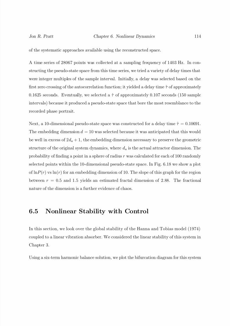
8/13/2019 Vibration Control for Chatter Suppression with Application to Boring Bars
http://slidepdf.com/reader/full/vibration-control-for-chatter-suppression-with-application-to-boring-bars 135/193

8/13/2019 Vibration Control for Chatter Suppression with Application to Boring Bars
http://slidepdf.com/reader/full/vibration-control-for-chatter-suppression-with-application-to-boring-bars 136/193

8/13/2019 Vibration Control for Chatter Suppression with Application to Boring Bars
http://slidepdf.com/reader/full/vibration-control-for-chatter-suppression-with-application-to-boring-bars 137/193
Jon R. Pratt Chapter 6. Nonlinear Dynamics 116
Figure 6.12: Comparison of nonlinear response curves obtained from analog simulation
with the results obtained from a six-term harmonic balance solution when (a) τ = 1/75
and (b) τ = 1/60. Solid lines denote stable periodic solutions and dotted lines denote
unstable periodic solutions determined in the previous analysis. Diamonds denote pointsobtained via analog computer.

8/13/2019 Vibration Control for Chatter Suppression with Application to Boring Bars
http://slidepdf.com/reader/full/vibration-control-for-chatter-suppression-with-application-to-boring-bars 138/193
Jon R. Pratt Chapter 6. Nonlinear Dynamics 117
0 1 2 3 4 5 6 7 810
-6
10-5
10-4
10-3
10-2
frequency
Figure 6.13: Power spectrum of the response for τ = 1/60 and w = 0.200.

8/13/2019 Vibration Control for Chatter Suppression with Application to Boring Bars
http://slidepdf.com/reader/full/vibration-control-for-chatter-suppression-with-application-to-boring-bars 139/193
Jon R. Pratt Chapter 6. Nonlinear Dynamics 118
-4 -2 0 2 4
x 10-3
-5
0
5(a)
x (in)
v ( i n / s e c )
-4 -2 0 2 4
x 10-3
-5
0
5(b)
x (in)
0 0.02 0.04-4-2024
x 10-3
(c)
time (sec)
x ( i n )
0 2 4 6 810
-6
10-4
10-2
(d)
frequency
-4 -2 0 2 4
x 10-3
-5
0
5(e)
x (in)
v ( i n / s e c )
-4 -2 0 2 4
x 10-3
-5
0
5(f)
x (in)
0 0.02 0.04-4-20
24
x 10-3
(g)
time (sec)
x ( i n )
0 2 4 6 810
-6
10-4
10-2
(h)
frequency
Figure 6.14: The phase portraits (a) and (e), the Poincare sections (b) and (f ), the time
histories (c) and (g), and the power spectra (d) and (h) of the attractors obtained when
τ = 1/75 and w = 0.060 and w = 0.136, respectively.
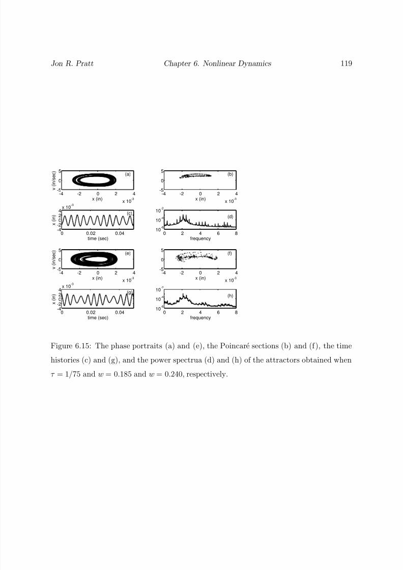
8/13/2019 Vibration Control for Chatter Suppression with Application to Boring Bars
http://slidepdf.com/reader/full/vibration-control-for-chatter-suppression-with-application-to-boring-bars 140/193
Jon R. Pratt Chapter 6. Nonlinear Dynamics 119
-4 -2 0 2 4
x 10-3
-5
0
5(a)
x (in)
v ( i n / s e c )
-4 -2 0 2 4
x 10-3
-5
0
5(b)
x (in)
0 0.02 0.04-4-2024
x 10-3
(c)
time (sec)
x ( i n )
0 2 4 6 810
-6
10-4
10-2
(d)
frequency
-4 -2 0 2 4
x 10-3
-5
0
5(e)
x (in)
v ( i n / s e c )
-4 -2 0 2 4
x 10-3
-5
0
5(f)
x (in)
0 0.02 0.04-4-20
24
x 10-3
(g)
time (sec)
x ( i n )
0 2 4 6 810
-6
10-4
10-2
(h)
frequency
Figure 6.15: The phase portraits (a) and (e), the Poincare sections (b) and (f ), the time
histories (c) and (g), and the power spectrua (d) and (h) of the attractors obtained when
τ = 1/75 and w = 0.185 and w = 0.240, respectively.
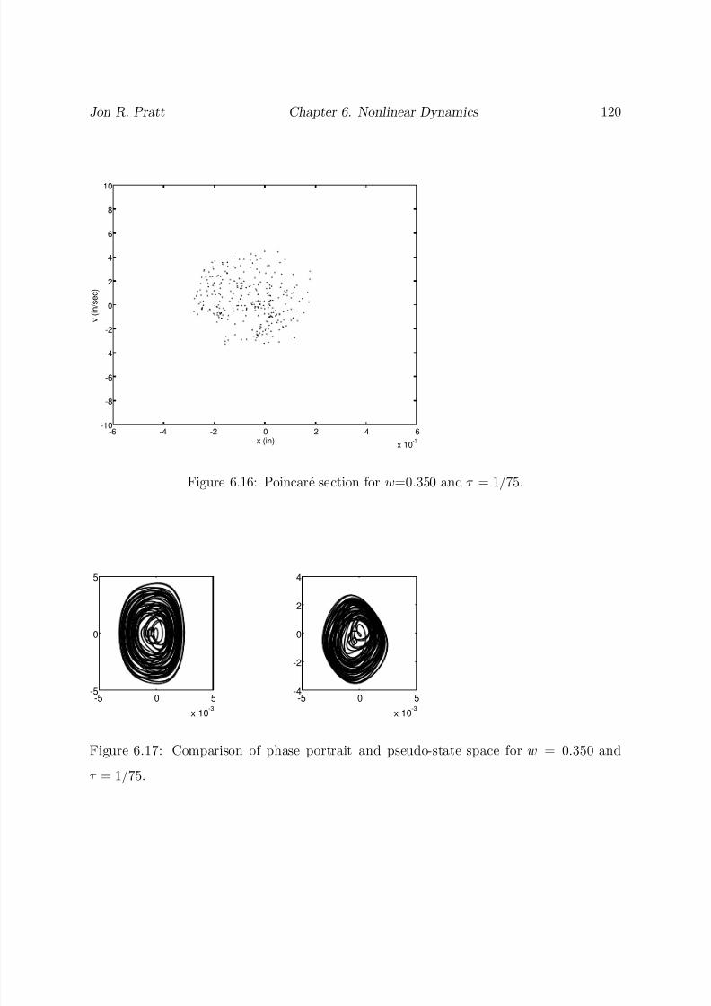
8/13/2019 Vibration Control for Chatter Suppression with Application to Boring Bars
http://slidepdf.com/reader/full/vibration-control-for-chatter-suppression-with-application-to-boring-bars 141/193
Jon R. Pratt Chapter 6. Nonlinear Dynamics 120
-6 -4 -2 0 2 4 6
x 10-3
-10
-8
-6
-4
-2
0
2
4
6
8
10
x (in)
v ( i n / s e c )
Figure 6.16: Poincare section for w=0.350 and τ = 1/75.
-5 0 5
x 10-3
-5
0
5
-5 0 5
x 10-3
-4
-2
0
2
4
Figure 6.17: Comparison of phase portrait and pseudo-state space for w = 0.350 and
τ = 1/75.

8/13/2019 Vibration Control for Chatter Suppression with Application to Boring Bars
http://slidepdf.com/reader/full/vibration-control-for-chatter-suppression-with-application-to-boring-bars 142/193
Jon R. Pratt Chapter 6. Nonlinear Dynamics 121
-2.5 -2 -1.5 -1 -0.5 0 0.5 1 1.5-8
-7
-6
-5
-4
-3
-2
-1
0
ln(r)
l n [ P ( r ) ]
d=10
Figure 6.18: Pointwise dimension for an embedding dimension of 10.
0.00 0.20 0.40 0.60
w
0.0000
0.0010
0.0020
a
Figure 6.19: Bifurcation diagram showing the amplitude of the fundamental chatter har-
monic a as a function of the effective width of cut w. The solid curve was obtained using
a six-term harmonic balance. The circles indicate points obtained via analog simulation.

8/13/2019 Vibration Control for Chatter Suppression with Application to Boring Bars
http://slidepdf.com/reader/full/vibration-control-for-chatter-suppression-with-application-to-boring-bars 143/193
Chapter 7
A Two-Degree-of-Freedom
Boring-Bar Chatter Model
We now take up the two-degree-of-freedom model for boring-bar dynamics that was pre-
sented in Chapter 2.
Recall, that the proposed system can be expressed mathematically as
x1 + 2ζ 1ω1 x1 + ω21x2 = −γ 1w[η(x1 − x1τ ) + ν (x2 − x2τ )] (7.1)
x2 + 2ζ 2ω2 x2 + ω22x2 = −γ 2w[η(x1 − x1τ ) + ν (x2 − x2τ )] (7.2)
where the coordinates x1 and x2 correspond to tool motions directed in the principal modal
directions and the constants are as defined previously. In the remainder of this chapter,
we develop this model more thoroughly, incorporate nonlinearities in the fashion of Hanna
and Tobias (1974), explore the local stability of the combined system, and illustrate the
existence of multiple chatter modes, as observed experimentally, via numerical integration
of the complete system.
122

8/13/2019 Vibration Control for Chatter Suppression with Application to Boring Bars
http://slidepdf.com/reader/full/vibration-control-for-chatter-suppression-with-application-to-boring-bars 144/193
Jon R. Pratt Chapter 7. 2DOF Boring bar Chatter Model 123
7.1 Modeling
So far, the system lacks any nonlinearity that would clamp the chatter oscillations and
produce limit-cycle type behavior. Taking our cue from Hanna and Tobias (1974), we
include both structural and cutting force nonlinearities and modify the linear model as
follows:
x1 + 2ζ 1ω1 x1 + 2ξ 1 x1 + ω21 [x1 + f 1(x1)]
= −γ 1wη [(x1 − µ1x1τ ) + g1(x1 − µ1x1τ )]
+ν [(x2 − µ2x2τ ) + g2(x2 − µ2x2τ )] (7.3)
x2 + 2ζ 2ω2 x2 + 2ξ 2 x2 + ω22 [x2 + f 2(x2)] =
−γ 2wη [(x1 − µ1x1τ ) + g1(x1 − µ1x1τ )]
+ν [(x2 − µ2x2τ ) + g2(x2 − µ2x2τ )] (7.4)
where f n(xn) is a function describing the structural nonlinearity in the nth modal coordi-
nate, gn(xn − µnxnτ ) is a function describing the regenerative cutting force nonlinearity
in each coordinate, ξ n is the damping due to the cutting process in each coordinate, γ n is
an influence coefficient describing the component of the differential cutting force projected
onto each coordinate, η is a coefficient describing the degree to which motions in the x1
direction contribute to the differential cutting force, ν is a coefficient describing the degree
to which motions in the x2 direction contribute to the differential cutting force, and µn
describes the degree of cut overlap in each direction.
7.1.1 Geometric Considerations
The model is based on knowledge of the direction of the mean cutting force, the angles
that it makes with the tool coordinates, and the angles these coordinates make with an

8/13/2019 Vibration Control for Chatter Suppression with Application to Boring Bars
http://slidepdf.com/reader/full/vibration-control-for-chatter-suppression-with-application-to-boring-bars 145/193
Jon R. Pratt Chapter 7. 2DOF Boring bar Chatter Model 124
orthogonal cutting plane. We have noted in the experimental work that the orientations of
the mean cutting force and the orthogonal cutting plane tend to change with the width of
cut and will attempt to illustrate this phenomenon heuristically via consideration of two
limiting cases.
In Fig. 7.1 (b), we illustrate the case encountered for extremely light cuts where the width
of cut is less than the tool nose radius. Under these conditions, the chip flows smoothly
from the tool in a direction oriented between 60 and 90 degrees to the machined surface
in the plane of the tool for small feedrates. Tool motions normal to the machined surface
have a componenent that modulates the chip thickness while the affect of motions in the
tangential direction is small, but significant.
In Fig. 7.1 (a), we illustrate the case where the width of cut is much greater than the
tool nose radius. Under these conditions, the chip flows smoothly away from the tool in a
direction normal to the transient surface in the plane of the tool for small feedrates. The
orthogonal cutting plane is now rotated by as much as 90 degrees from that of the shallow
cutting condition, and tool motions normal to the machined surface no longer modulate
the chip thickness. Instead, tool motions tangential to the machined surface indirectly
modulate the chip thickness and give rise to regenerative chatter of type B as defined by
Tobias (1965).
The seeming change in the orientation of the plane in which cutting might be characterized
as nearly “orthogonal” is due to the finite nose radius of the insert. Clearly, the effective
tool lead angle can vary from 0 to ≈ 90 as the chip width is decreased below a value
corresponding to the radius of the insert (0.01 in this case). Similar observations regarding
the chip flow in oblique, multi-edged cutting geometries were originally reported by Stabler
(1964).
For certain cutting geometries, it might appear that the two transverse vibratory modes of

8/13/2019 Vibration Control for Chatter Suppression with Application to Boring Bars
http://slidepdf.com/reader/full/vibration-control-for-chatter-suppression-with-application-to-boring-bars 146/193
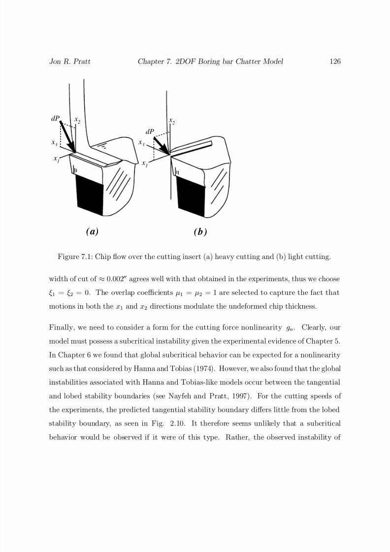
8/13/2019 Vibration Control for Chatter Suppression with Application to Boring Bars
http://slidepdf.com/reader/full/vibration-control-for-chatter-suppression-with-application-to-boring-bars 147/193
Jon R. Pratt Chapter 7. 2DOF Boring bar Chatter Model 126
dP
dP
x1
x2
x3
x1
x2
x3
(a) (b)
Figure 7.1: Chip flow over the cutting insert (a) heavy cutting and (b) light cutting.
width of cut of ≈ 0.002 agrees well with that obtained in the experiments, thus we choose
ξ 1 = ξ 2 = 0. The overlap coefficients µ1 = µ2 = 1 are selected to capture the fact that
motions in both the x1 and x2 directions modulate the undeformed chip thickness.
Finally, we need to consider a form for the cutting force nonlinearity gn. Clearly, our
model must possess a subcritical instability given the experimental evidence of Chapter 5.
In Chapter 6 we found that global subcritical behavior can be expected for a nonlinearity
such as that considered by Hanna and Tobias (1974). However, we also found that the global
instabilities associated with Hanna and Tobias-like models occur between the tangential
and lobed stability boundaries (see Nayfeh and Pratt, 1997). For the cutting speeds of
the experiments, the predicted tangential stability boundary differs little from the lobed
stability boundary, as seen in Fig. 2.10. It therefore seems unlikely that a subcritical
behavior would be observed if it were of this type. Rather, the observed instability of

8/13/2019 Vibration Control for Chatter Suppression with Application to Boring Bars
http://slidepdf.com/reader/full/vibration-control-for-chatter-suppression-with-application-to-boring-bars 148/193
Jon R. Pratt Chapter 7. 2DOF Boring bar Chatter Model 127
Figure 7.2: Tool response for a “heavy” orthogonal cut when w = 0.1, speed is 230 rpm,
and the feedrate is 0.0024 ipr.
the light cutting experiments seems to be more like a locally subcritical one capable of
producing jumps for widths of cut below the tangential boundary. Such a behavior was
encountered by Shi and Tobias (1986) in some of their face milling experiments and was
recently analyzed by Stepan (1997) in his reconsideration of Shi and Tobias’s work.
Stepan (1997), working from the results of Shi and Tobias (1986), suggested that a lo-
cal subcritical-type instability can exist when the sign of the cubic term in the ployno-
mial expression for the cutting-force nonlinearity proposed by Hanna and Tobias (1974) is
changed from negative to positive. Physically, the results of Stepan (1997) suggest that
a softening-type cutting-force characteristic can produce locally subcritical behavior in a
single-degree-of-freedom model for dynamic cutting.
In Figure 7.3 we show the static cutting forces measured using a dynamometer that was
incorporated as part of the smart-tool fixture. These results were obtained by shortening
the boring-bar overhang, disconnecting the actuators, and measuring the cutting forces for
a series of widths of cut at a fixed speed of 200 surface feet per minute (approximately

8/13/2019 Vibration Control for Chatter Suppression with Application to Boring Bars
http://slidepdf.com/reader/full/vibration-control-for-chatter-suppression-with-application-to-boring-bars 149/193
Jon R. Pratt Chapter 7. 2DOF Boring bar Chatter Model 128
180 rpm) and a feedrate of 0.0024 ipr. The zero point is imposed to indicate loss of tool
engagment.
We see a nearly linear dependence on cut width in the direction of the tool speed, as is
typical, however the forces normal (radial) to the machined surface appear to have a more
complex structure. A “knee” in the radial cutting force occurs as the width of cut exceeds
0.01. This is precisely the point where the width of cut begins to exceed the tool nose
radius. It provides a further corroboration of our hypothesized mean force variation with
width of cut. We also note that the data indicates an inflection point near a width of cut
0.002. Radial force measurements in this region were inconsistent, but it appears that
the force achieves a plateau in a fashion that might be modeled with a locally softening
characteristic.
It seems, on the basis of the observed stability and the measured static cutting forces,
that our model for light cutting conditions below 0.005 should employ some form of a
softening-type cutting-force characteristic.
7.1.3 A Model for Heavy Cuts
To model the tool accelerations of Fig. 5.13, we let ξ 1/ω1 + ζ 1 = 0.2, ξ 2 = 0, γ 1 =
cos(π/3)ω21
ksλ1
, γ 1 = cos (π/6)ω21
ksλ1
, η = 0.495, ν = −0.24, µ1 = 1, µ2 = 1, and assume the
following functional relations for the structural and cutting force nonlinearities:
f 1(x1) = 0 if x1 < 0
5x1 otherwise(7.7)
f 2(x2) = 10x22 + 300x3
2 (7.8)
gn(xn − µnxnτ ) = 5.7(xn − µnxnτ )2 − 3700(xn − µnxnτ )
3 (7.9)

8/13/2019 Vibration Control for Chatter Suppression with Application to Boring Bars
http://slidepdf.com/reader/full/vibration-control-for-chatter-suppression-with-application-to-boring-bars 150/193
Jon R. Pratt Chapter 7. 2DOF Boring bar Chatter Model 129
0 0.02 0.04 0.060
5
10
15
20
25
30
inches
l b s
* Vertical
+ Radial
Figure 7.3: Static cutting forces as a function of depth of cut.
The regenerative cutting force as well as the structural nonlinearities are identical in form
to those used by Hanna and Tobias (1974). In this case we ignore the issue of the type of
instability and focus merely on producing an accurate representation of the tool chatter.
The damping in the x1 direction was observed to be qualitatively “high” in the time traces
of the impact response of the tool measured during stable cutting at lower speeds (see Fig.
5.6); hence, a very substantial effect of process damping is incorporated by using a large
value of ξ 1. The overlap coefficient µ1 = 1 was selected to capture the fact that motions
in the x1 direction modulate the undeformed chip cross-section in a complex fashion that
depends on the previous tool position. On the other hand, motions in the x2 direction
modulate the chip thickness via a penetration effect labeled type-B chatter by Tobias
(1965). The sign of the coefficient ν was chosen to be negative based on the tendency of
the tangential chatter frequency to be lower than ω2, which would not be the case if ν > 0.
Perhaps the most unconventional feature of the model is the bilinear structural stiffness

8/13/2019 Vibration Control for Chatter Suppression with Application to Boring Bars
http://slidepdf.com/reader/full/vibration-control-for-chatter-suppression-with-application-to-boring-bars 151/193
Jon R. Pratt Chapter 7. 2DOF Boring bar Chatter Model 130
represented by the function f 1(x1). This function was chosen to produce the unsymmetric
tool motions that were evident in the time traces at this width of cut and speed. We
hypothesize that the tool does not so much cut the workpiece in the x1 direction as plow
into it, giving rise to the near impact-type oscillations observed in this coordinate during
the experiments.
7.2 Stability
We consider the conditions prevalent during the light cutting scenario because this will
define the lower bound of stable widths of cut. Furthermore, from a practical standpoint,
chatter is most detrimental during a finish cut, where the emphasis is on bringing a part
to a precise dimensional tolerance and surface finish.
The linear stability boundary for this case was determined in Chapter 2 and plotted for
the two-degree-of-freedom model in Fig. 2.10. In this section, we consider the transition
from stable to unstable cutting by deriving the normal form for the Hopf bifurcation point
using the methods described in Chapter 6.
First, we write the equations of motion. Based on the light cutting model, we have
xk + 2ζ kωk xk + ω2kF k(xk) = −γ kwF c[(x1 − x1τ ), (x2 − x2τ )] (7.10)
where k = 1, 2,
F k(xk) = xk + β k2x2k + β k3x3
k, (7.11)
and
F c[(x1 − x1τ ), (x2 − x2τ )] = η[(x1 − x1τ ) + α12(x1 − x1τ )2 + α13(x1 − x1τ )
3]
+ ν [(x2 − x2τ ) + α22(x2 − x2τ )2 + α23(x2 − x2τ )
3] (7.12)

8/13/2019 Vibration Control for Chatter Suppression with Application to Boring Bars
http://slidepdf.com/reader/full/vibration-control-for-chatter-suppression-with-application-to-boring-bars 152/193
Jon R. Pratt Chapter 7. 2DOF Boring bar Chatter Model 131
Due to the presence of both cubic and quadratic nonlinearities, the perturbation analysis
must be performed using either the method of multiple scales or the generalized method of
averaging, or a center manifold technique (Stepan, 1989). In this Dissertation, we choose
a multiple-scales approach (Nayfeh, 1973, 1981).
Following the developments of Chapter 6, we introduce a fast time scale T 0 = t and a slow
time scale T 2 = 2t and seek a third-order expansion in the form
xk = xk1(T 0, T 2) + 2xk2(T 0, T 2) + 3xk3(T 0, T 2) + · · · (7.13)
We express the time derivatives as
d
dt = D0 + 2D2 + · · · and
d2
dt2 = D2
0 + 22D0D2 + · · · (7.14)
where
Dn = ∂
∂T n(7.15)
Moreover, we let
w = wc + 2w2 + · · · (7.16)
Substituting Eqs. (7.13)-(7.16) into Eqs. (7.10) and equating coefficients of like powers of
, we obtain
Order :
D20xk1 + 2ζ kωkD0xk1 + ω2
kxk1 + γ kwc[η(x11 − x11τ ) + ν (x21 − x21τ )] = 0 (7.17)
Order 2:
D20xk2 + 2ζ kωkD0xk2 + ω2
kxk2+ γ kwc[η(x12− x12τ ) + ν (x22 − x22τ )] =
−ω2kβ k2x2
k1 − γ kwc[ηα12(x11 − x11τ )2
+να22(x21 − x21τ )2] (7.18)

8/13/2019 Vibration Control for Chatter Suppression with Application to Boring Bars
http://slidepdf.com/reader/full/vibration-control-for-chatter-suppression-with-application-to-boring-bars 153/193
Jon R. Pratt Chapter 7. 2DOF Boring bar Chatter Model 132
Order 3:
D20xk3 + 2ζ kωkD0xk3+ ω2
kxk3 + γ kwc[η(x13− x13τ ) + ν (x23 − x23τ )] =
−ω2k(2β k2xk1xk2 + β k3x3
k1) − 2ζ kωkD2xk1 − 2D0D2xk1
−γ kwcη[2α12(x11− x11τ )(x12 − x12τ ) + α13(x11 − x11τ )3]
+ν [2α22(x21 − x21τ )(x22 − x22τ ) + α23(x21 − x21τ )3]
−γ kw2[η(x11 − x11τ ) + ν (x21 − x21τ )] (7.19)
We now define a delay operator
LD[x(t), τ ] = x(t− τ ) (7.20)
and rewrite the equations making use of matrix operator notation as
Order :
Lx11 x12T = 0 (7.21)
Order 2:
Lx12 x22T =
−ω21β 12x2
11 − γ 1wcηα12[(1 − LD)x11]2 + να22[(1 − LD)x21]2
−ω22β 22x2
21 − γ 2wcηα12[(1 − LD)x11]2 + να22[(1 − LD)x21]2
(7.22)
8/13/2019 Vibration Control for Chatter Suppression with Application to Boring Bars
http://slidepdf.com/reader/full/vibration-control-for-chatter-suppression-with-application-to-boring-bars 154/193

8/13/2019 Vibration Control for Chatter Suppression with Application to Boring Bars
http://slidepdf.com/reader/full/vibration-control-for-chatter-suppression-with-application-to-boring-bars 155/193
Jon R. Pratt Chapter 7. 2DOF Boring bar Chatter Model 134
x21 = A1(T 2)b1eiωcT 0 + cc, and x21τ = A1(T 2)b1eiωc(T 0−τ ) + cc (7.26)
where b1 can be obtained by various methods through consideration of the linear problem.
Previously, we used a Laplace transform approach, and we stick with that method here.
We take the Laplace transform of Eq. (7.21) and, assuming zero initial conditions, express
x21 in terms of x11 via the transfer function
H (s) = − γ 2wcη(1 − esτ )
s2 + 2ζ 2ω2s + ω22 + γ 2wcν (1 − esτ )
(7.27)
At the Hopf bifurcation point,
b1 = H (iωc), and b1 = H (−iωc) (7.28)
Substituting Eqs. (7.25) and (7.26) into Eq. (7.22) we obtain
Lx12 x22T =
−A21ω2
1β 12 + γ 1wc(1 − e−iωcτ )2[ηα12 + να22b21]ei2ωcT 0
−A1 A1ω2
1β 12 + γ 1wc(1 − e−iωcτ )(1− eiωcτ )[ηα12 + να22b1b1]
−A21ω2
2β 22 + γ 2wc(1 − e−iωcτ )2[ηα12 + να22b21]ei2ωcT 0
−A1 A1ω2
2β 22 + γ 2wc(1 − e−iωcτ )(1− eiωcτ )[ηα12 + να22b1b1]
+ cc (7.29)
which we express in a more compact fashion as
Lx12 x22T = −A2
1
p1
p2
ei2ωcT 0 − A1
A1
q 1
q 2
+ cc (7.30)
where
pk = ω2kβ k2 + γ kwc(1 − e−iωcτ )2[ηα12 + να22b21], k = 1, 2 (7.31)
q k = ω2kβ k2 + γ kwc(1 − e−iωcτ )(1 − eiωcτ )[ηα12 + να22b1b1], k = 1, 2 (7.32)
We observe that the inhomogeneous terms are nonsecular and either constant or porpor-
tional to e2iωcT 0. To obtain a solution at this order, we assume a particular solution of the

8/13/2019 Vibration Control for Chatter Suppression with Application to Boring Bars
http://slidepdf.com/reader/full/vibration-control-for-chatter-suppression-with-application-to-boring-bars 156/193
Jon R. Pratt Chapter 7. 2DOF Boring bar Chatter Model 135
form
xk2 = A21P kei2ωcT 0 + QkA1 A1 + cc, k = 1, 2 (7.33)
and substitute it into Eq. (7.30). Equating coefficients of like terms from either side of the
resulting equation yields
G(2iωc)
P 1
P 2
= −
p1
p2
(7.34)
Qk = −q kω2
k
(7.35)
where in general
G(iω) =
ω21 − ω2 + 2iζ 1ω1ω
+γ 1wcη(1− e−iωcτ )γ 1wcν (1 − e−iωcτ )
γ 2wcη(1 − e−iωcτ )ω22 − ω2 + 2iζ 2ω2ω
+γ 2wcν (1 − e−iωcτ )
(7.36)
Solving for the coefficients P k, we obtain
P 1
P 2
= −G−1(2iωc)
p1
p2
(7.37)
Substituting Eq. (7.33) into Eq. (7.23), performing some algebraic manipulations, and
defining some new variables, we have

8/13/2019 Vibration Control for Chatter Suppression with Application to Boring Bars
http://slidepdf.com/reader/full/vibration-control-for-chatter-suppression-with-application-to-boring-bars 157/193
Jon R. Pratt Chapter 7. 2DOF Boring bar Chatter Model 136
Lx13 x23T =
−2(ζ 1ω1 + iωc)A
1
−γ 1w2(η + νc1)(1 − e−iωcτ )A1
−Λ1A21 A1
−2(ζ 2ω2 + iωc)A
1
−γ 2w2(η + νc1)(1 − e−iωcτ )A1
−Λ2A21 A1
eiωcT 0 + cc + NST (7.38)
where the prime denotes differentiation with respect to T 2 and
Λ1 = ω21(2β 12P 1 + 3β 13 + 2β 12Q1)
+γ 1wcη[2α12P 1(1− e−2iωcτ )(1 − eiωcτ )
+3α13(1 − e−iωcτ )2(1− eiωcτ )]
+ν [2α22P 2b1(1 − e−2iωcτ )(1− eiωcτ )
+3α23b
2
1
¯b1(1 − e
−iωcτ
)
2
(1 − e
iωcτ
)] (7.39)
Λ2 = ω22(2β 22P 2c1 + 3β 23c21c1 + 2β 22c1Q2)
+γ 2wcη[2α12P 1(1− e−2iωcτ )(1 − eiωcτ )
+3α13(1 − e−iωcτ )2(1− eiωcτ )]
+ν [2α22P 2b1(1 − e−2iωcτ )(1− eiωcτ )
+3α23b21b1(1 − e−iωcτ )2(1 − eiωcτ )] (7.40)
To determine the solvability conditions, we seek a particular solution free of secular terms
in the form
x13 = K 1eiωcT 0, and x23 = K 2eiωcT 0 (7.41)

8/13/2019 Vibration Control for Chatter Suppression with Application to Boring Bars
http://slidepdf.com/reader/full/vibration-control-for-chatter-suppression-with-application-to-boring-bars 158/193
Jon R. Pratt Chapter 7. 2DOF Boring bar Chatter Model 137
Substituting Eq. (7.41) into Eq. (7.38), we have
G(iωc)
K 1
K 2
=
−2(ζ 1ω1 + iωc)A
1 − γ 1w2(η + νc1)(1− e−iωcτ )A1 − Λ1A21 A1
−2(ζ 2ω2 + iωc)A
1 − γ 2w2(η + νc1)(1− e−iωcτ )A1 − Λ2A21 A1
(7.42)
Equations (7.42) constitute a system of two inhomogeneous algebraic equations for K 1 and
K 2. Their homogeneous parts have a nontrivial solution as we learned in Chapter 2. Hence,
the solvability condition is obtained by setting the determinant of the following augmented
matrix equal to zero. The result is
det
ω21 − ω2
c + 2iζ 1ω1ωc
+γ 1wcη(1 − e−iωcτ )
−2(ζ 1ω1 + iωc)A
1
−γ 1w2(η + νc1)(1− e−iωcτ )A1
−Λ1A21 A1
γ 2wcη(1 − e−iωcτ )
−2(ζ 2ω2 + iωc)A
1
−γ 2w2(η + νc1)(1− e−iωcτ )A1
−Λ2A21 A1
= 0 (7.43)
This condition yields
Γ1A
1 + Γ2A1 + Γ3A21 A1 = 0 (7.44)
where
Γ1 = Γ1r + iΓ1i
= 2(ζ 1ω1 + iωc)(γ 2wcη(1 − e−iωcτ ))
−2c1(ζ 2ω2 + iωc)(ω21 − ω2
c + 2iζ 1ω1ωc + γ 1wcη(1 − e−iωcτ )) (7.45)
Γ2 = Γ2r + iΓ2i
= γ 1γ 2w2wcη(1 − e−iωcτ )2(η + νc1)
−γ 2w2(η + νc1)(1− e−iωcτ )(ω21 − ω2
c + 2iζ 1ω1ωc + γ 1wcη(1 − e−iωcτ )) (7.46)
8/13/2019 Vibration Control for Chatter Suppression with Application to Boring Bars
http://slidepdf.com/reader/full/vibration-control-for-chatter-suppression-with-application-to-boring-bars 159/193
Jon R. Pratt Chapter 7. 2DOF Boring bar Chatter Model 138
Γ3 = Γ3r + iΓ3i
= Λ1γ 2wcη(1− e−iωcτ ) − 2Λ2(ω21 − ω2
c + 2iζ 1ω1ωc + γ 1wcη(1− e−iωcτ )) (7.47)
Introducing the polar transformation
A1 = 1
2aeiβ (7.48)
into the solvability condition Eq. (7.44) and separating real and imaginary parts, we obtain
the normal form
a = c1w2a + c2a3 (7.49)
aβ = c3w2a + c4a3 (7.50)
where
c1 = −Γ1rΓ2r + Γ1iΓ2i
Γ21r + Γ2
1i
(7.51)
c2 = −1
4
Γ1rΓ3r + Γ1iΓ3i
Γ21r + Γ2
1i
(7.52)
c3 = −Γ1rΓ2i − Γ1iΓ2r
Γ21r + Γ2
1i(7.53)
c4 = −1
4
Γ1rΓ3i − Γ1iΓ3r
Γ21r + Γ2
1i
(7.54)
As discussed in Chapter 6, the qualitative behavior of the local instability is determined
by the sign of the coefficient c2 in the above normal form. Plugging in the model values
from Section 7.1.2 we find that a transition from a locally supercritical behavior to a locally
subcritical behavior occurs as chi changes from negative to positive.
Stepan (1997) obtained a similar normal form and results for a single-degree-of-freedom
nonlinear cutting model. He considered a softening-type cutting force characteristic, essen-
tially changing the sign of coefficient α3 in the Hanna and Tobias model, and used center
manifold reduction to obtain the normal form. He did not address the global behavior of
8/13/2019 Vibration Control for Chatter Suppression with Application to Boring Bars
http://slidepdf.com/reader/full/vibration-control-for-chatter-suppression-with-application-to-boring-bars 160/193
Jon R. Pratt Chapter 7. 2DOF Boring bar Chatter Model 139
the system in the post-bifurcation region in a rigorous fashion, but argued that at some
point the tool must leave the cut, and that one could reasonably expect that the region
where jump phenomena could occur would be limited to a parameter space where widths
of cut produced unstable limit cycles of amplitudes less than the mean chip thickness. He
obtained an expression for the amplitude of the unstable limit cycles from consideration of
his normal form, an exercise we carry out now for our system.
We seek the amplitude of the limit cycles as predicted by the local analysis. This may be
simply obtained by setting a = 0 in Eq. (7.49). Then the steady state amplitude of the
resulting limit cycles can be determined as a function of width of cut from the expression
w = wc − c2c1
a2 (7.55)
We let χ = −4.25α3 and use Eq. (7.55) to generate the bifurcation diagram plotted in Fig.
(7.4).
In the simulations, we confirm that a subcritical bifurcation due to cutting force nonlinearity
exists and that it requires another substantial nonlinearity if bounded periodic motions are
to result. We hypothesize that, in order to predict the post-bifurcation behavior, it is
necessary to extend the model to incoroprate the effect of the tool leaving the cut, as
implied by Stepan (1997) and considered by Tlusty (1985), Shi and Tobias (1986), and
Kondo etal. (1981).
7.3 Simulated Responses
In the following simulations we use the dynamic tool properties that were identified for the
Smart Tool during the experimental testing period of August, 1996. Thus, the frequencies
and dampings are f 2 = 493 Hz and ζ 2 ≈ 0.03 and f 1 = 365 Hz and ζ 1 ≈ 0.02.
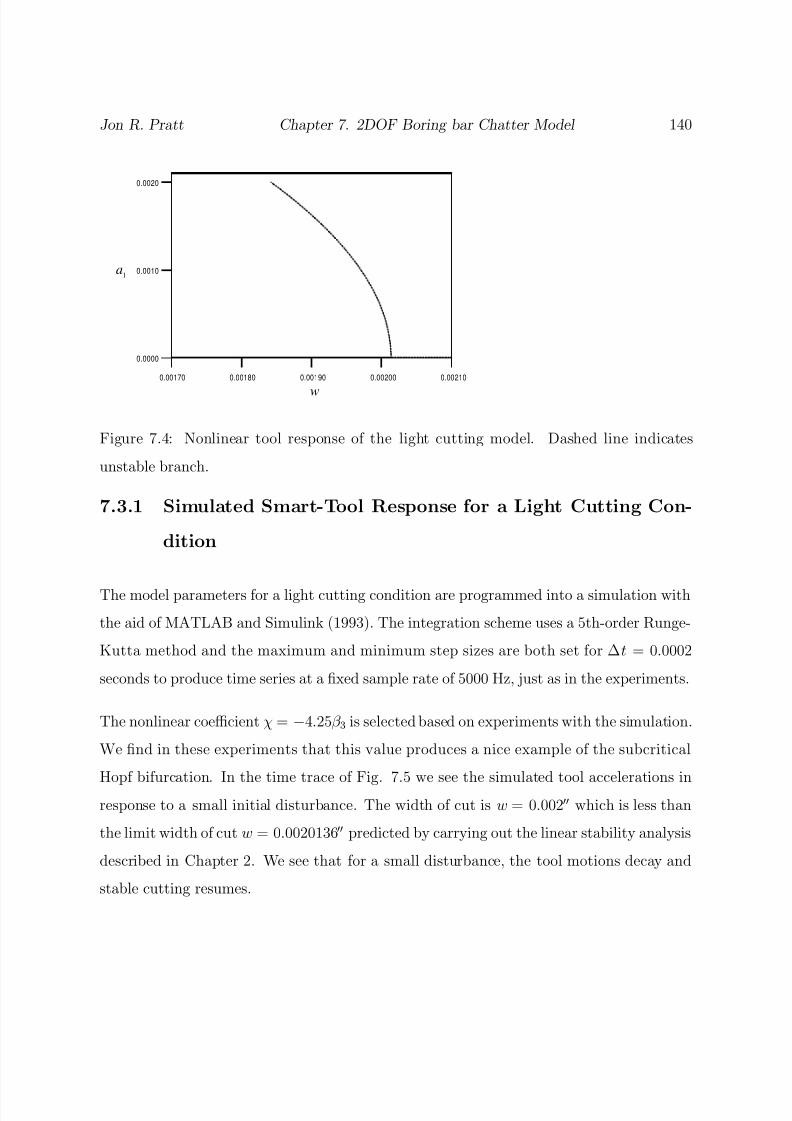
8/13/2019 Vibration Control for Chatter Suppression with Application to Boring Bars
http://slidepdf.com/reader/full/vibration-control-for-chatter-suppression-with-application-to-boring-bars 161/193
Jon R. Pratt Chapter 7. 2DOF Boring bar Chatter Model 140
a1
w
0.00170 0.00180 0.00190 0.00200 0.00210
0.0000
0.0010
0.0020
Figure 7.4: Nonlinear tool response of the light cutting model. Dashed line indicates
unstable branch.
7.3.1 Simulated Smart-Tool Response for a Light Cutting Con-
dition
The model parameters for a light cutting condition are programmed into a simulation with
the aid of MATLAB and Simulink (1993). The integration scheme uses a 5th-order Runge-
Kutta method and the maximum and minimum step sizes are both set for ∆t = 0.0002
seconds to produce time series at a fixed sample rate of 5000 Hz, just as in the experiments.
The nonlinear coefficient χ = −4.25β 3 is selected based on experiments with the simulation.
We find in these experiments that this value produces a nice example of the subcritical
Hopf bifurcation. In the time trace of Fig. 7.5 we see the simulated tool accelerations in
response to a small initial disturbance. The width of cut is w = 0.002 which is less than
the limit width of cut w = 0.0020136 predicted by carrying out the linear stability analysis
described in Chapter 2. We see that for a small disturbance, the tool motions decay and
stable cutting resumes.

8/13/2019 Vibration Control for Chatter Suppression with Application to Boring Bars
http://slidepdf.com/reader/full/vibration-control-for-chatter-suppression-with-application-to-boring-bars 162/193
Jon R. Pratt Chapter 7. 2DOF Boring bar Chatter Model 141
In Fig. 7.6 a larger initial disturbance is introduced with x1 = 0.008 (which is really
outside of the cut) and x2 = 0.0005. Tool oscillations are seen to grow in amplitude with
time. The solution is obviously diverging, confirming our analytical prediction of a locally
subcritical-type instability.
We speculate that for light cuts with locally subcritical-type instabilities, the dominant
nonlinearity necessary to produce bounded tool motions is that produced by the tool leav-
ing the cut, as has been commonly cited in the literature. The question arises as to whether
or not the nonlinearity produced by the tool leaving the cut is sufficient by itself to account
for the subcritical behavior of machine tools, as was once speculated in Hooke and Tobias
(1964), or whether it is necessary to include a softening characteristic in the cutting force,
as is speculated here and by Stepan (1997). At present, we have no answer for this ques-
tion, but we believe it can be determined by looking at the stability of periodic solutions
that result from models such as those suggested by Tlusty, where the only nonlinearity
considered is that of the tool leaving the cut. Presumably, a harmonic-balance approach
like that undertaken by Shi and Tobias (1986) for the discontinuous cutting force could
be employed to obtain a periodic solution and then the stability could be ascertained us-
ing Floquet theory, as was demonstrated in Chapter 6. Alternately, we could attack the
problem numerically by extending the shooting method to retarded dynamical systems.
7.3.2 Simulated Smart Tool Response for a Heavy cutting Con-
dition
The model parameters for a heavy cutting condition are programmed into a simulation with
the aid of MATLAB and Simulink (1993). The integration scheme uses a 5th-order Runge-
Kutta method and the maximum and minimum step sizes are both set for ∆t = 0.0001
seconds to produce time series at a fixed sample rate of 10000 Hz. The simulation is started
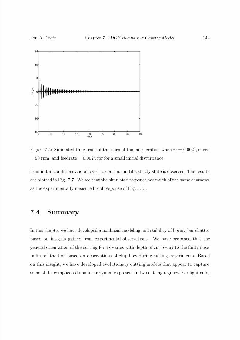
8/13/2019 Vibration Control for Chatter Suppression with Application to Boring Bars
http://slidepdf.com/reader/full/vibration-control-for-chatter-suppression-with-application-to-boring-bars 163/193
Jon R. Pratt Chapter 7. 2DOF Boring bar Chatter Model 142
0 5 10 15 20 25 30 35 40-15
-10
-5
0
5
10
15
time
a n
g s
Figure 7.5: Simulated time trace of the normal tool acceleration when w = 0.002, speed
= 90 rpm, and feedrate = 0.0024 ipr for a small initial disturbance.
from initial conditions and allowed to continue until a steady state is observed. The results
are plotted in Fig. 7.7. We see that the simulated response has much of the same character
as the experimentally measured tool response of Fig. 5.13.
7.4 Summary
In this chapter we have developed a nonlinear modeling and stability of boring-bar chatter
based on insights gained from experimental observations. We have proposed that the
general orientation of the cutting forces varies with depth of cut owing to the finite nose
radius of the tool based on observations of chip flow during cutting experiments. Based
on this insight, we have developed evolutionary cutting models that appear to capture
some of the complicated nonlinear dynamics present in two cutting regimes. For light cuts,
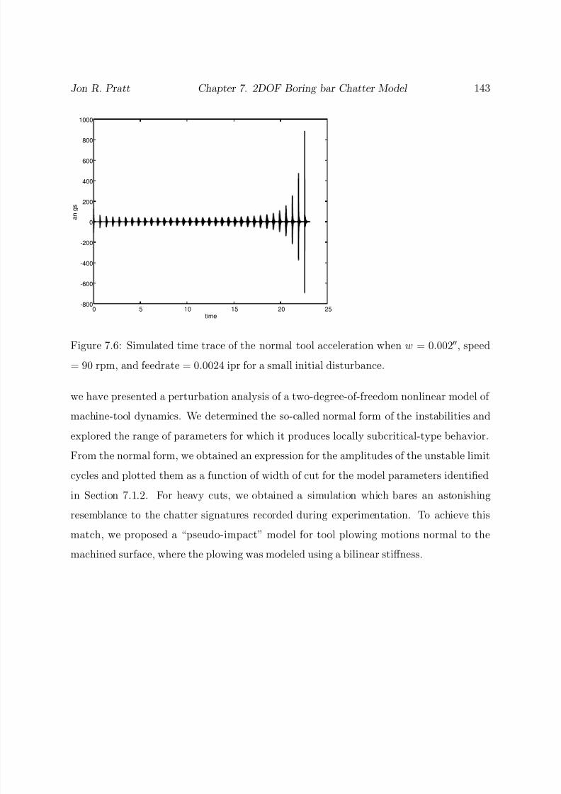
8/13/2019 Vibration Control for Chatter Suppression with Application to Boring Bars
http://slidepdf.com/reader/full/vibration-control-for-chatter-suppression-with-application-to-boring-bars 164/193
Jon R. Pratt Chapter 7. 2DOF Boring bar Chatter Model 143
0 5 10 15 20 25-800
-600
-400
-200
0
200
400
600
800
1000
time
a n
g s
Figure 7.6: Simulated time trace of the normal tool acceleration when w = 0.002, speed
= 90 rpm, and feedrate = 0.0024 ipr for a small initial disturbance.
we have presented a perturbation analysis of a two-degree-of-freedom nonlinear model of
machine-tool dynamics. We determined the so-called normal form of the instabilities and
explored the range of parameters for which it produces locally subcritical-type behavior.
From the normal form, we obtained an expression for the amplitudes of the unstable limit
cycles and plotted them as a function of width of cut for the model parameters identified
in Section 7.1.2. For heavy cuts, we obtained a simulation which bares an astonishing
resemblance to the chatter signatures recorded during experimentation. To achieve this
match, we proposed a “pseudo-impact” model for tool plowing motions normal to the
machined surface, where the plowing was modeled using a bilinear stiffness.

8/13/2019 Vibration Control for Chatter Suppression with Application to Boring Bars
http://slidepdf.com/reader/full/vibration-control-for-chatter-suppression-with-application-to-boring-bars 165/193
Jon R. Pratt Chapter 7. 2DOF Boring bar Chatter Model 144
1 1.02 1.04-100
0
100
time (secs)
a n
g
s
0 500 1000 1500 2000
-100
-50
0
50
freq (Hz)
d B g
s
478 Hz
1 1.02 1.04-100
0
100
time (secs)
a t g s
0 500 1000 1500 2000-100
0
100
freq (Hz)
d B g
s
478 Hz
0 500 1000 1500 2000-50
0
50
freq. (Hz)
d B s
0 500 1000 1500 20000
0.5
1
freq. (Hz)
c o h
e r e n c e
Figure 7.7: Simulated time traces, autospectra, cross-spectrum, and coherence of the nor-
mal and tangential tool accelerations when w = 0.03, speed = 210 rpm, and feedrate
= 0.0024 ipr.
8/13/2019 Vibration Control for Chatter Suppression with Application to Boring Bars
http://slidepdf.com/reader/full/vibration-control-for-chatter-suppression-with-application-to-boring-bars 166/193
Chapter 8
Nonlinear Control Techniques for
Chatter Reduction
Working from nonlinear single-degree-of-freedom models for chatter, we develop two ideas
that show promise as alternatives or supplements to linear chatter mitigation, providedthat a structural control system of sufficient bandwidth and dynamic range can be devised.
The first idea is based on the observation that the amplitude of post-bifurcation limit cycles
due to regenerative chatter is determined completely by the nonlinearities present in the
combined machine-tool and cutting-process dynamics. Thus, by applying proper nonlinear
feedback through the structural control, one can effectively limit the size of limit-cycle
vibrations. Also, for a system such as that considered by Hanna and Tobias (1974), the
nonlinear feedback can be used to achieve a global bifurcation control. We demonstrate,
by feeding back a term proportional to the cube of the tool velocity, that one can change
the structure of the machine-tool stability from globally subcritical, or unsafe, to globally
supercritical, or safe.
145

8/13/2019 Vibration Control for Chatter Suppression with Application to Boring Bars
http://slidepdf.com/reader/full/vibration-control-for-chatter-suppression-with-application-to-boring-bars 167/193
Jon R. Pratt Chapter 8. Nonlinear Control 146
The second idea is an open-loop control strategy based on the well-known “quench” phe-
nomenon that occurs in the forced response of self-excited systems (see Nayfeh and Mook
1979). Here, for the first time, we show that a quench phenomenon exists for time-delay sys-
tems. We inject a signal with frequency incommensurate to the chatter frequency into the
bifurcation control feedback signal. The combination of the high-frequency forced response
with cubic velocity feedback is shown to quench chatter vibrations to acceptably small
amplitudes, thereby extending the operating range of a Hanna and Tobias-like machine
tool.
8.1 Global Bifurcation Control via Nonlinear State
Feedback
We observed experimentally in Chapter 5 and theoretically in Chapters 6 and 7 that the
local and global dynamics of machining processes can exhibit subcritical, or unsafe in-
stabilities, characterized by jump phenomena. In this section, we propose a method for
eliminating this behavior by ensuring that an appropriate nonlinear term is included in the
equation of motion. For this Dissertation, we suppose that the force represented by this
term is available via direct nonlinear feedback control using an actuator, though clearly it
would be desirable to design the tool in such a fashion that the force arises naturally as
part of the cutting process.
The stability we wish to alter is, in some instances, part of the global dynamics. Recall,
that locally, the stability of a hardening-type cutting force is characterized by a supercrit-
ical Hopf bifurcation, but that the subsequent small-amplitude periodic motions quickly
lose stability via a cyclic-fold bifurcation that cannot be detected using a local analysis.
Nevertheless, we begin our theoretical consideration of the problem by examining the effect
8/13/2019 Vibration Control for Chatter Suppression with Application to Boring Bars
http://slidepdf.com/reader/full/vibration-control-for-chatter-suppression-with-application-to-boring-bars 168/193
Jon R. Pratt Chapter 8. Nonlinear Control 147
of cubic-velocity feedback on the structure of the nonlinear normal form for such a system.
In essence, we seek clues as to how much more supercritical we must make the local bifurca-
tion in order to preserve its supercritical structure in the global response. We then use the
harmonic-balance technique developed in Chapter 6 to generate nonlinear response curves,
or bifurcation diagrams, for various levels of nonlinear feedback to ascertain the minimum
gain required to achieve the desired change in the form of the bifurcation. We then present
digital-computer simulation results for comparison with the stability predictions of the
harmonic-balance analysis.
8.1.1 Theory for High-Speed Machining
The current thrust in machine-tool research is towards ever higher spindle speeds; the
so-called high-speed machining centers. This trend is motivated by two factors. First,
higher speeds and feeds result in greater production capacity and faster time to market.
Second, tool forces tend to decline with increasing speed while the stability against regen-
erative chatter increases, as evidenced by the spreading of the stability lobes. However,
the perceived gain in cutting stability with increased speed (and hence reduced time delay)
may be dubious in the presence of subcritical instabilities. Here, we consider a hypotheti-
cal high-speed machining operation and develop a theortical framework for implementing
bifurcation control via nonlinear feedback.
The model is that of Hanna and Tobias (1974). We consider the case of high-speed ma-
chining where the regenerative phase lag ωcτ is between 3π/2 and 7π/2, or the instability
is constrained to occur within the first lobe. We presume that either passive or active
control has been employed to increase the tool damping by an order of magnitude so that
ξ new = 10ξ new . Thus, our hypothetical system is more representative of the coming state-
of-the-art than the typical shop lathe that was employed in the experimental portion of
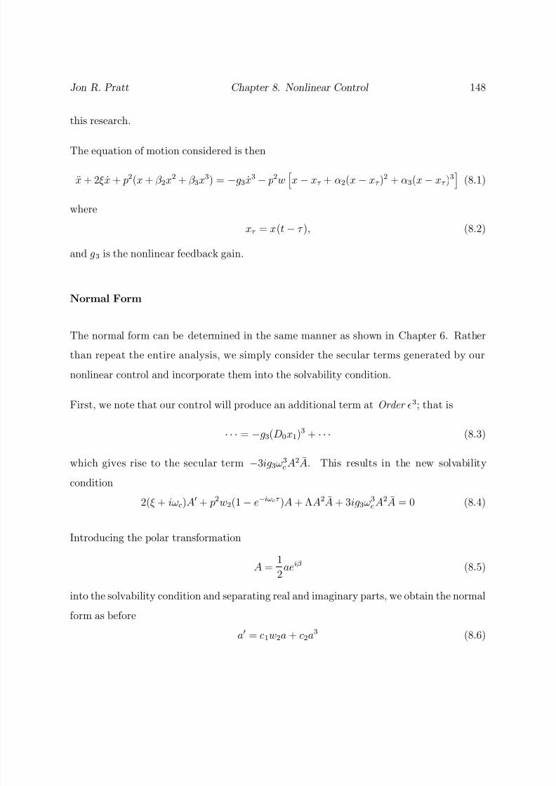
8/13/2019 Vibration Control for Chatter Suppression with Application to Boring Bars
http://slidepdf.com/reader/full/vibration-control-for-chatter-suppression-with-application-to-boring-bars 169/193
Jon R. Pratt Chapter 8. Nonlinear Control 148
this research.
The equation of motion considered is then
x + 2ξ x + p2(x + β 2x2 + β 3x3) = −g3x3− p2wx − xτ + α2(x − xτ )
2 + α3(x− xτ )3
(8.1)
where
xτ = x(t − τ ), (8.2)
and g3 is the nonlinear feedback gain.
Normal Form
The normal form can be determined in the same manner as shown in Chapter 6. Rather
than repeat the entire analysis, we simply consider the secular terms generated by our
nonlinear control and incorporate them into the solvability condition.
First, we note that our control will produce an additional term at Order 3; that is
· · · = −g3(D0x1)3 + · · · (8.3)
which gives rise to the secular term −3ig3ω3c A2 A. This results in the new solvability
condition
2(ξ + iωc)A + p2w2(1− e−iωcτ )A + ΛA2 A + 3ig3ω3c A2 A = 0 (8.4)
Introducing the polar transformation
A = 1
2aeiβ (8.5)
into the solvability condition and separating real and imaginary parts, we obtain the normal
form as before
a = c1w2a + c2a3 (8.6)

8/13/2019 Vibration Control for Chatter Suppression with Application to Boring Bars
http://slidepdf.com/reader/full/vibration-control-for-chatter-suppression-with-application-to-boring-bars 170/193
Jon R. Pratt Chapter 8. Nonlinear Control 149
aβ = c3w2a + c4a3 (8.7)
where now the coefficient c2 is modified such that
c2 = − 1
8(ξ 2 + ω2c )
(ξ Λr + ωcΛi + 3g3ω4c ) (8.8)
The qualitative behavior near the Hopf bifurcation can be determined by the sign of c2.
Here, we see that the choice of nonlinear velocity feedback has given us the ability to ensure
that c2 is negative, for the case when softening-type cutting forces might otherwise produce
a subcritical Hopf bifurcation, and to increase the degree to which c2
is negative in the case
when hardening-type cutting force nonlinearities combined with structural nonlinearities
produce a global subcritical instability. The former case is traditional bifurcation control,
as discussed in Nayfeh and Balachandran (1995). The latter case is an extension to the
concept of global instability.
Stability Analysis
It appeared in our earlier analysis of the linear chatter control that the application of
a vibration-absorber-type control that enhances the tool damping could also affect the
global stability. This is true in part. What occurs is that the global subcritical instability
becomes substantially smaller in proportion to the tangential stability boundary, at least
for the rotational speeds previously considered. However, at high rotational speeds we
find that the effect once again becomes significant. This is important from a technological
standpoint because the latest thrust in machine-tool dynamics research is towards high-speed machining. Spindles capable of tens of thousands of rpm’s are being brought into
service by the major airframe manufacturers with little understanding yet of the dynamic
implications.
In Fig. 8.1 we see the results of a global stability analysis for the case 1/τ = 749.9 and
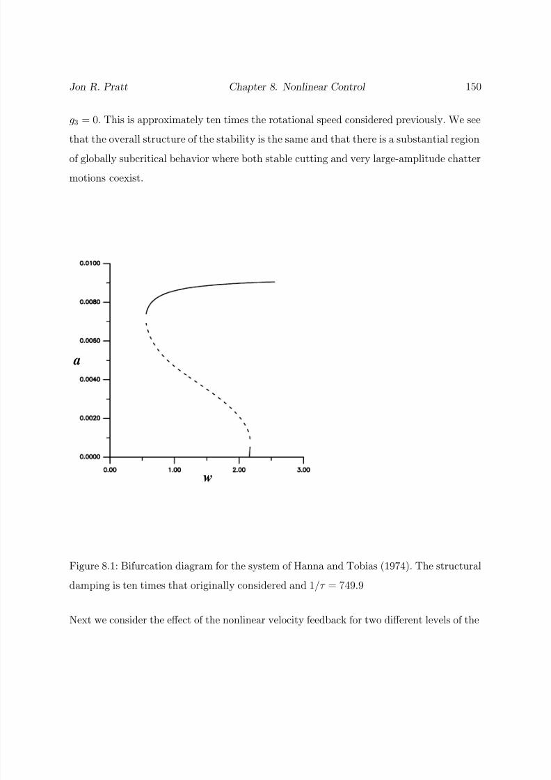
8/13/2019 Vibration Control for Chatter Suppression with Application to Boring Bars
http://slidepdf.com/reader/full/vibration-control-for-chatter-suppression-with-application-to-boring-bars 171/193
Jon R. Pratt Chapter 8. Nonlinear Control 150
g3 = 0. This is approximately ten times the rotational speed considered previously. We see
that the overall structure of the stability is the same and that there is a substantial region
of globally subcritical behavior where both stable cutting and very large-amplitude chatter
motions coexist.
a
w
Figure 8.1: Bifurcation diagram for the system of Hanna and Tobias (1974). The structural
damping is ten times that originally considered and 1/τ = 749.9
Next we consider the effect of the nonlinear velocity feedback for two different levels of the
8/13/2019 Vibration Control for Chatter Suppression with Application to Boring Bars
http://slidepdf.com/reader/full/vibration-control-for-chatter-suppression-with-application-to-boring-bars 172/193
Jon R. Pratt Chapter 8. Nonlinear Control 151
gain g3. The results are shown in Fig. 8.2. It appears from this analysis that, for nonlinear
feedback gains in excess of 10, the cyclic fold is eliminated and that the transistion to
chatter has been made a smooth function of the effective width of cut.
a
w
g=103
g=53
Figure 8.2: Comparison of the nonlinear tool response with and without bifurcation control
for two different levels of cubic velocity feedback.
8/13/2019 Vibration Control for Chatter Suppression with Application to Boring Bars
http://slidepdf.com/reader/full/vibration-control-for-chatter-suppression-with-application-to-boring-bars 173/193
Jon R. Pratt Chapter 8. Nonlinear Control 152
8.1.2 Simulation
In this section we consider the response of the system before and after application of non-
linear feedback control when g3 = 10. We use MATLAB and Simulink (1993) to integrate
the equation of motion and consider two cases with and without nonlinear feedback. The
first case we consider is when the effective width of cut w = 2, which, according to a linear
stability analysis, produces stable, chatter-free cutting. The second case we consider is in
the post-bifurcation regime when w = 2.3.
We see in the phase portrait and time trace of Figs. 8.3 (a) and (b) that the uncontrolled
tool response to a small initial condition decays to the trivial solution, while in Figs. 8.3
(c) and (d) we see that for a larger initial condition the tool motion grows to a stable limit
cycle. We see that the controlled response in Fig. 8.3 (d) and (e) is stable for the initial
condition that previously produced limit cycle behavior.
Finally, we show phase portraits in Figure 8.4 of the simulated response when w = 2.3,
which is beyond the linearly established limit width of cut. The nonlinear feedback greatly
reduces the severity of chatter, as evidenced by the considerable reduction in the size of
the limit cycle.
8.2 Quench Control
We note that the previously considered bifurcation control has the desired effect of elimi-nating subcritical instability, while also attenuating the size of limit cycles that occur in the
post-bifurcation region. In this section, we consider an open-loop control strategy known
as quench control that in conjunction with the bifurcation control can further attenuate
the size of the limit cycles.
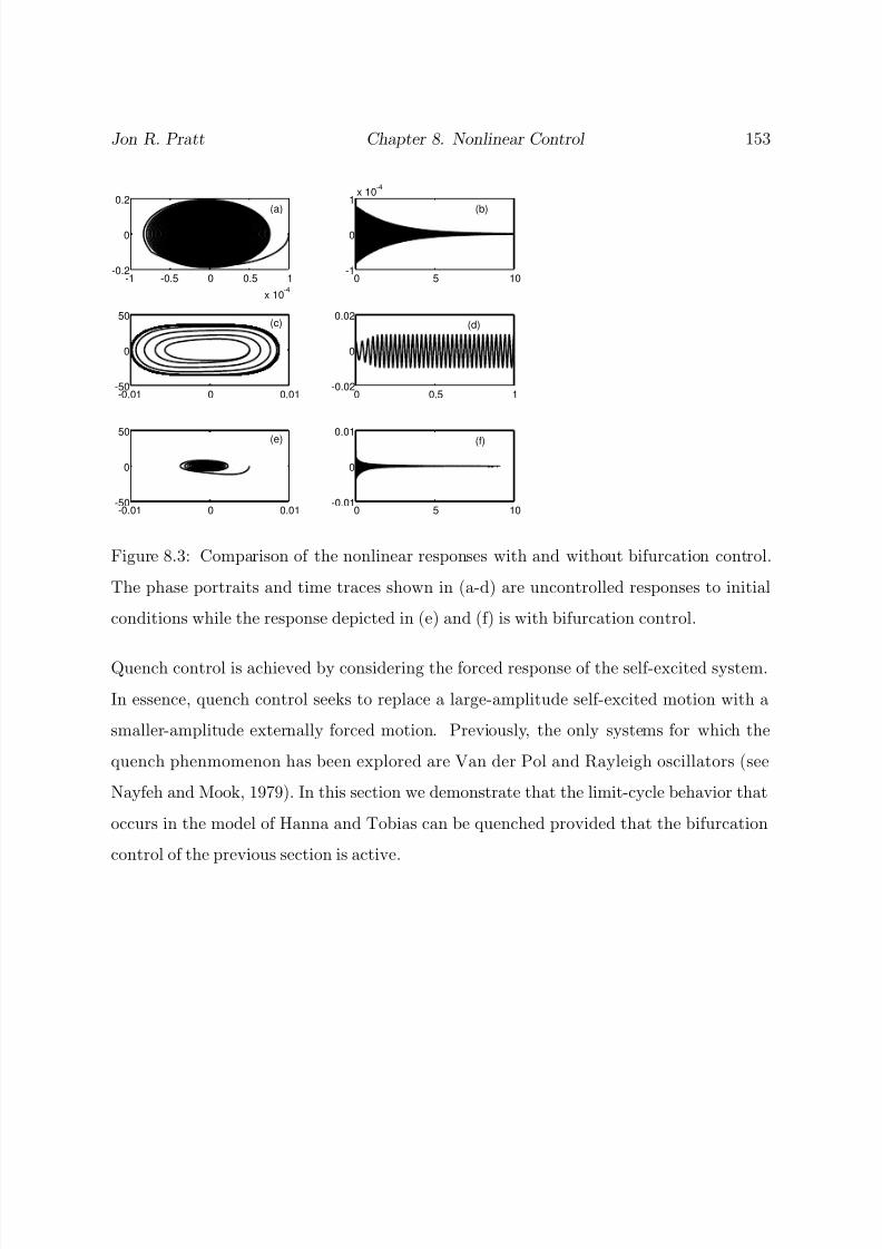
8/13/2019 Vibration Control for Chatter Suppression with Application to Boring Bars
http://slidepdf.com/reader/full/vibration-control-for-chatter-suppression-with-application-to-boring-bars 174/193

8/13/2019 Vibration Control for Chatter Suppression with Application to Boring Bars
http://slidepdf.com/reader/full/vibration-control-for-chatter-suppression-with-application-to-boring-bars 175/193
Jon R. Pratt Chapter 8. Nonlinear Control 154
-0.01 0 0.01-50
-40
-30
-20
-10
0
10
20
30
40
50
(a)
-0.01 0 0.01-50
-40
-30
-20
-10
0
10
20
30
40
50
(b)
Figure 8.4: Comparison of the phase portraits produced by the nonlinear response of the
tool in the x1 modal coordinate without bifurcation control (a) and with bifurcation control
(b).
8.2.1 Theory
To illustrate the concept, we augment the previously considered model for high-speed
machining as follows:
x+2ξ x+ p2(x+β 2x2+β 3x3) = −g3x3− p2wx − xτ + α2(x − xτ )
2 + α3(x − xτ )3
+f cos(Ωt)
(8.9)
where g3 is the nonlinear feedback gain for bifurcation control and f cos(Ωt) is the forcing
function that acts on the tool where the forcing frequency Ω is assumed to be incommen-
surate with the chatter frequency ωc determined during the course of the analysis.
Due to the presence of both cubic and quadratic nonlinearities, the perturbation analysis
must be performed using either the method of multiple scales or the generalized method of

8/13/2019 Vibration Control for Chatter Suppression with Application to Boring Bars
http://slidepdf.com/reader/full/vibration-control-for-chatter-suppression-with-application-to-boring-bars 176/193
Jon R. Pratt Chapter 8. Nonlinear Control 155
averaging (Nayfeh, 1973, 1981). In this Dissertation, we choose a multiple-scales approach.
Using the method of multiple scales (Nayfeh, 1973, 1981), we introduce a fast time scale
T 0 = t and a slow time scale T 2 = 2t and seek a third-order expansion in the form
x = x1(T 0, T 2) + 2x2(T 0, T 2) + 3x3(T 0, T 2) + · · · (8.10)
Moreover, we let
w = wc + 2w2 + · · · (8.11)
Substituting Eqs. (8.10) and (8.11) into Eq. (8.9) and equating coefficients of like powers
of , we obtain
Order :
D20x1 + 2ξD0x1 + p2x1 + p2wc(x1 − x1τ ) = f cos(ΩT 0) (8.12)
Order 2:
D20x2 + 2ξD0x2 + p
2
x2 + p2
wc(x2 − x2τ ) = − p2
β 2x21 − p
2
wcα2(x1 − x1τ )2
(8.13)
Order 3:
D20x3 + 2ξD0x3 + p2x3 + p2wc(x3 − x3τ ) =−2D0D2x1 − 2ξD2x1 − p2w2(x1 − x1τ )
−2 p2β 2x1x2 − 2 p2wcα2(x1 − x1τ )(x2 − x2τ )
− p2β 3x31 − p2wcα3(x1 − x1τ )
3 − g3(D0x1)3(8.14)
The solution of Eq. (8.12) can be expressed as
x1 = A(T 2)eiωcT 0 + λeiΩT 0 + cc, and x1τ = A(T 2)eiωc(T 0−τ ) + λeiΩ(T 0−τ ) + cc (8.15)
where
λ = f
2( p2 − Ω2 + 2iξ Ω + wc p2(1 − e−iΩτ )) (8.16)

8/13/2019 Vibration Control for Chatter Suppression with Application to Boring Bars
http://slidepdf.com/reader/full/vibration-control-for-chatter-suppression-with-application-to-boring-bars 177/193
Jon R. Pratt Chapter 8. Nonlinear Control 156
and ωc is the chatter frequency at the Hopf bifurcation point. Substituting Eq. (8.15) into
Eq. (8.13) and solving for x2, we obtain
x2 = − p2A2Γ1e2iωcT 0−Γ2A A− p2λ2Γ3e2iΩT 0−Γ4λλ− p2AλΓ5ei(ωc+Ω)T 0− p2AλΓ6ei(ωc−Ω)T 0+cc
(8.17)
where
Γ1 = β 2 + wcα2(1 − e−iωcτ )2
p2 − 4ω2c + 4iωcξ + p2wc(1 − e−2iωcτ )
(8.18)
Γ2 = β 2 + wcα2(1 − e−iωcτ )(1 − eiωcτ ) (8.19)
Γ3 = β
2 + w
cα2(1 − e−iΩτ )2
p2 − 4Ω2 + 4iΩξ + p2wc(1− e−2iΩτ ) (8.20)
Γ4 = β 2 + wcα2(1 − e−iΩτ )(1 − eiΩτ ) (8.21)
Γ5 = β 2 + wcα2(1− e−iωcτ )(1 − e−iΩτ )
p2 − 4(ωc + Ω)2 + 4i(ωc + Ω)ξ + p2wc(1− e−i(ωc+Ω)τ ) (8.22)
Γ6 = β 2 + wcα2(1− e−iωcτ )(1 − eiΩτ )
p2 − 4(ωc − Ω)2 + 4i(ωc − Ω)ξ + p2wc(1− e−i(ωc−Ω)τ ) (8.23)
Substituting Eqs. (8.15) and (8.17) into Eq. (8.14) and eliminating the terms that lead to
secular terms, we obtain the solvability condition
2(ξ + iωc)A + p2w2(1 − e−iωcτ )A + χAλλ + ΛA2 A + i3g3ω3c A2 A = 0 (8.24)
where
χ = χr + iχi
=−2 p2β 2(2Γ4 + p2Γ5 + p2Γ6) + 6 p2β 3
−2 p4wcα2[Γ5(1 − e−i(ωc+Ω)τ )(1− eiΩτ ) + Γ6(1 − e−i(ωc−Ω)τ )(1− e−iΩτ )
+6 p2wcα3(1 − e−iωcτ )(1− e−iΩτ )(1 − eiΩτ ) − 6ig3ωcΩ2, (8.25)
Λ = Λr + iΛi
=−2 p2β 2( p2Γ1 + 2Γ2) + 3 p2β 3 − 2 p4wcα2Γ1(1 − eiωcτ )(1− e−2iωcτ )
+3 p2wcα3(1 − e−iωcτ )2(1 − eiωcτ ), (8.26)

8/13/2019 Vibration Control for Chatter Suppression with Application to Boring Bars
http://slidepdf.com/reader/full/vibration-control-for-chatter-suppression-with-application-to-boring-bars 178/193
Jon R. Pratt Chapter 8. Nonlinear Control 157
and Λr, Λi, χr, and χi are real constants.
Introducing the polar transformation
A = 1
2aeiβ (8.27)
into Eq. (8.24) and separating real and imaginary parts, we obtain the normal form
a = c1w2a + c2a3 (8.28)
aβ
= c3w2a + c4a3
(8.29)
where
c1 = − 1
2(ξ 2 + ω2c )
[ p2ξ (1 − cos ωcτ ) + p2ωc sin ωcτ + λλ(ξχr + ωcχi)] (8.30)
c2 = − 1
8(ξ 2 + ω2c )
(ξ Λr + ωcΛi + 3g3ω4c ) (8.31)
c3 = − 1
2(ξ 2 + ω2c )
[ p2ξ sin ωcτ − p2ωc(1 − cos ωcτ ) + λλ(ξχi − ωcχr)] (8.32)
c4 = − 1
8(ξ 2 + ω2c )
(ξ Λi − ωcΛr) (8.33)
Machining instability only exists when c1 > 0, otherwise the amplitude of the limit cycles
decay exponentially to the trivial solution regardless of the nonlinearities. We see that the
addition of quench control has produced terms in the coefficient c1 that are proportional
to the forcing level λ. Thus, for forcing levels such that
[ p2ξ (1 − cos ωcτ ) + p2ωc sin ωcτ + λλ(ξχr + ωcχi)] > 0 (8.34)
the limit cycles are quenched, leaving only the forced response.

8/13/2019 Vibration Control for Chatter Suppression with Application to Boring Bars
http://slidepdf.com/reader/full/vibration-control-for-chatter-suppression-with-application-to-boring-bars 179/193
Jon R. Pratt Chapter 8. Nonlinear Control 158
8.2.2 Simulation
The model is programmed into a numerial simulation with the aid of MATLAB and
Simulink (1993). The integration uses a 5th-order Runge-Kutta method and the maxi-
mum and minimum step sizes are both set for ∆t = 0.00001 seconds to produce time series
with a fixed sample rate of 100000 Hz. The model parameters are as before with τ = 749.9
and w = 2.3. The results are plotted in Fig. 8.5.
Beginning at time t = 0, the simulation starts from an initial tool displacement of x = 0.002
that quickly grows to a large-amplitude limit cycle. At time t = 0.5 the bifurcation control
is activated with a gain g3 = 10. The limit cycle is seen to shrink considerably in amplitude.
Next, at time t = 1.5 the quench control is activated with f = 0.0035/386Ω2 and Ω = 10000.
The quenching force causes a further reduction in the tool response. In Fig. 8.6 we compare
the steady-state tool responses before and after application of the quench control where a
smaller time window has been employed to reveal the change in amplitude and frequency.
Clearly, we have successfully exchanged a large-amplitude self-excited motion for a higher-
frequency, lower-amplitude forced response.
8.3 Summary
In this chapter we have demonstrated two nonlinear chatter-control techniques on a model
for high-speed machining. We show that by introducing nonlinear velocity feedback in themachine-tool structure it is possible to eliminate subcritical instabilities from the machine-
tool operating envelope. Furthermore, such a control strategy has been shown to greatly
attenuate the size of the post-bifurcation limit cycles.

8/13/2019 Vibration Control for Chatter Suppression with Application to Boring Bars
http://slidepdf.com/reader/full/vibration-control-for-chatter-suppression-with-application-to-boring-bars 180/193
Jon R. Pratt Chapter 8. Nonlinear Control 159
0 0.2 0.4 0.6 0.8 1 1.2 1.4 1.6 1.8
-0.01
0
0.01
time
Figure 8.5: Illustration of the nonlinear tool responses as control is applied. First, nonlinear
velocity feedback is applied at t = 0.5, then the quench control is “turned on” at t = 1.0.
A quench control technique has also been proposed as an open-loop method to enhance
the performance of the nonlinear feedback in the post-bifurcation regime. Quench control
requires high-frequency, large-amplitude, non-resonant forcing be applied to the tool to
convert self-excited limit cycles to small-amplitude, forced oscillations. In other words, we
convert the system from autonomous to nonautonomous behavior. At first glance, this
seems an inefficient way to attack a vibration problem. However, from a technological
standpoint it is fairly easy to conceive of a small “buzzer” embedded in the boring bar that
is simply turned on if vibrations exceed a threshold. In fact, in cutting processes where
nonlinear friction effects dominate, one can expect that quench control could be employed
without resort to any feedback at all, making it a very simple and economical alternative
to the more traditional, linear approach employed in the Smart Tool.
Regardless of the merits of the quench phenomenon as a control strategy, the theoretical

8/13/2019 Vibration Control for Chatter Suppression with Application to Boring Bars
http://slidepdf.com/reader/full/vibration-control-for-chatter-suppression-with-application-to-boring-bars 181/193
Jon R. Pratt Chapter 8. Nonlinear Control 160
0 1 2 3 4 5
x 10-3
-3
-2
-1
0
1
2x 10
-3
time
Figure 8.6: Comparison of the steady-state tool responses with and without quench control.
The dashed line is the tool motion with the active quench control.
results obtained should prove applicable in the area of ultrasonic machining, where the cut-
ting process is carried out using a tool that is forced to vibrate at frequencies corresponding
to the wave speed of the tool material. The forced response analysis can also be employed
to consider various resonant conditions that might exist due to external forcing. As noted
at the very beginning of the Dissertation, machine-tool chatter can result from forced vi-
brations. There are many instances when rotating imbalance or tool run out contribute
a periodic forcing to the tool that is detrimental to the part quality. One can reasonably
assume that these forced vibration problems are excacerbated by conditions at high spin-
dle speeds, and that the time when the problem of combined forced and self-excited tool
motions must be considered is fast approaching.
8/13/2019 Vibration Control for Chatter Suppression with Application to Boring Bars
http://slidepdf.com/reader/full/vibration-control-for-chatter-suppression-with-application-to-boring-bars 182/193
Chapter 9
Summary
In this Dissertation we have explored the dynamics and control of machine-tool vibrations
with particular attention to boring-bar chatter. We began with the classic models for
machine-tool vibrations and laid the foundation for a simple linear control strategy. Using
knowledge available from the smart structures research of the last decade, we devised aunique manufacturing research platform known as the Smart Tool to bring our control con-
cepts to fruition. The design, integration, and modeling of this device constituted a major
undertaking in itself, and is representative of the type of systems design, or mechatronic
engineering, that is playing an ever increasing role in the advancement of engineering sci-
ence and practice. The development of this platform constitutes a significant advancement
in the fields of manufacturing design engineering, smart structures design and analysis, and
applied controls.
We developed detailed models and simulations of the Smart Tool performance by adapt-
ing concepts from experimental modal analysis, classical controls, the mechanics of metal
removal, signal processing, and nonlinear dynamics as needed to facilitate our efforts. The
161

8/13/2019 Vibration Control for Chatter Suppression with Application to Boring Bars
http://slidepdf.com/reader/full/vibration-control-for-chatter-suppression-with-application-to-boring-bars 183/193
Jon R. Pratt Chapter 9. Summary 162
resulting reduced-order models capture the observed experimental behaviors with remark-
able accuracy, and the simulations, when combined with the experimental observations,
bring the complex dynamic character of boring-bar chatter into much sharper focus. The
experimental models of chatter greatly further our understanding of the complex machine-
tool vibration problem, a problem that has been at the heart of a global research effort for
the last forty years, and the experimental data base obtained can provide continued new
insights into chatter behavior in coupled oscillatory systems as it is further explored.
The analytical treatments of nonlinear machine-tool stability define the state-of-the art
and will be a valuable tool to other researchers in the years to come. In particular, the
treatments of the nonlinear stability of the two-degree-of-freedom problem, the application
of bifurcation control to affect both local and global change in the qualitative behavior of
a retarded dynamical system, the application of these concepts to high-speed machining,
and the treatment of the combination of time-delayed self-excitation and external forcing
to yield a quenching phenomenon are firsts that represent significant achievements in the
areas of manufacturing science, nonlinear dynamics, and controls.

8/13/2019 Vibration Control for Chatter Suppression with Application to Boring Bars
http://slidepdf.com/reader/full/vibration-control-for-chatter-suppression-with-application-to-boring-bars 184/193
References
163

8/13/2019 Vibration Control for Chatter Suppression with Application to Boring Bars
http://slidepdf.com/reader/full/vibration-control-for-chatter-suppression-with-application-to-boring-bars 185/193
Bibliography
[1] Armarego, E. J. A., and Brown, R. H., 1969, The Machining of Metals , Prentice-Hall,
New Jersey.
[2] Arnold, R. N., 1946, “The Mechanism of Tool Vibration in the Cutting of Steel,”
Proceedings, Institution of Mechanical Engineers , Vol. 154, p. 261.
[3] Boothroyd, G., 1975, Fundamentals of Metal Machining and Machine Tools ,
McGraw-Hill, New York.
[4] Bruner, A. M., Belvin, W. K., Horta, L. G., and Juang, J.-N., 1992, “Active Vibration
Absorber for the CSI Evolutionary Model: Design and Experimental Results,” J.
Guid., Cont., Dyn., Vol. 15, p. 1253.
[5] Campbell, M. E. and Crawley, E. F., 1997, “Actuator and Sensor Design for Con-
trolled Structures,” Proceedings of the 39th AIAA/ASME/ASCE/AHS Structures,
Structural Dynamics, and Materials Conference , AIAA Paper No. 97-1150.
[6] Davies, M. A., and Balachandran, B., 1996, “Impact Dynamics in the Milling of Thin-
Walled Structures,” 6th Conference on Nonlinear Vibrations, Stability, and Dynamics
of Structures , Blacksburg, VA.
[7] Den Hartog, J. P., 1985, Mechanical Vibrations , Dover, New York.
164
8/13/2019 Vibration Control for Chatter Suppression with Application to Boring Bars
http://slidepdf.com/reader/full/vibration-control-for-chatter-suppression-with-application-to-boring-bars 186/193
References 165
[8] Ewins, D. J., 1986, Modal Testing: Theory and Practice , Research Studies Press,
Ltd., Letchworth, England.
[9] Fanson, J. L., Blackwood, G. H., and Chu, C-C., 1989, “Active Member Control of
Precision Structures,” Proceedings of the 30th AIAA/ASME/ASCE/AHS Structures,
Structural Dynamics, and Materials Conference , AIAA Paper No. 89-1329.
[10] Fanson, J. L. and Caughey, T. K., 1987, “Positive Position Feedback Control for Large
Space Structures,” Proceedings of the 28th AIAA/ASME/ASCE/AHS Structures,
Structural Dynamics, and Materials Conference , AIAA Paper No. 87-0902.
[11] Gilsinn, D. E., and Davies, M., 1996, “Multi-Modal Nonlinear Dynamics in Machine
Tool Cutting Processes,” 6th Conference on Nonlinear Vibrations, Stability, and Dy-
namics of Structures , Blacksburg, VA.
[12] Goh, C. J. and Caughey, T. K., 1985, “On the Stability Problem Caused by Finite
Actuator Dynamics in the Control of Large Space Structures,” Int. J. Cont., Vol. 41,
p. 787.
[13] Grabec, I., 1988, “Chaotic Dynamics of the Cutting Process,” Int. J. Mach. Tools
Manuf., Vol. 28, p. 19.
[14] Hanna, N. H., and Tobias, S. A., 1974, “A Theory of Nonlinear Regenerative Chat-
ter,” ASME J. Eng. Indust., Vol. 96, p. 247.
[15] Hastings, W. F., Mathew, P., and Oxley, P. L. B., 1980, “A Machining Theory for
Predicting Chip Geometry, Cutting Forces etc. from Work Material and CuttingConditions,” Proc. R. Soc. Lond., Vol. A 371, p. 569.
[16] Hastings, W. F., Oxley, P. L. B., and Stevenson, M. G., 1971, “Assessing Machinabil-
ity From Fundamental Work Material Properties”, in Proceedings of the 12th MTDR
Conference , Manchester, England, p. 507.

8/13/2019 Vibration Control for Chatter Suppression with Application to Boring Bars
http://slidepdf.com/reader/full/vibration-control-for-chatter-suppression-with-application-to-boring-bars 187/193
References 166
[17] Hooke, C. J., and Tobias, S. A., 1964, “Finite Amplitude Instability-A New Type of
Chatter,” in Proceedings of the 4th International M.T.D.R. Conference , Manchester,
p. 97.
[18] Hopkins, D. A., 1976, Vibration Damping Assembly, U.S. Patent, No. 3938626.
[19] Johnson, C. D., 1970, “Further Study of the Linear Regulator with Disturbances-the
case of vector disturbances Satisfying a Linear Differential Equation,” Inst. Electri.
Electro. Eng. Trans. Auto. Cont., Vol. AC-15, p. 222.
[20] Johnson, C. D., 1971, “Accommodation of External Disturbances in Linear Regulator
and Servomechanism Problems,” Inst. Electri. Electro. Eng. Trans. Auto. Cont., Vol.
AC-16, p. 635.
[21] Juang, J.-N., and Phan, M., 1992, “Robust Controller Designs for Second- Order
Dynamic Systems: A Virtual Passive Approach,” J. Guid., Cont. Dyn., Vol. 15, No.
5, p. 1192.
[22] Kalpakjian, S., 1992, Manufacturing Engineering and Technology, Second Edition ,
Addison-Wesley, New York.
[23] Kelson, Z. Y., and Hsueh, W. C., 1996, “Suppression of Chatter in Inner-Diameter
Cutting,” JSME Int. J. Series C: Dyn., Cont. Robot., Design, Manuf., Vol. 39, no.
1, p. 25.
[24] King, R. I., 1985, Handbook of High Speed Machining Technology , Chapman and Hall,
New York.
[25] Kobayashi, S. and Thomsen, E. G., 1962, “Metal-Cutting Analysis-I and II,” ASME
J. Eng. Indust., Vol. 84, p. 63.

8/13/2019 Vibration Control for Chatter Suppression with Application to Boring Bars
http://slidepdf.com/reader/full/vibration-control-for-chatter-suppression-with-application-to-boring-bars 188/193
References 167
[26] Koeingsberger, F., and Tlusty, J., 1970, Machine Tool Structures , Vol. 1, Pergamon
Press, New Jersey.
[27] Kondo, Y., Kawano, O., and Sato, H., 1981, “Behavior of Self-Excited Chatter Due
to Multiple Regenerative Effect,” ASME J. Eng. Ind., Vol. 103, p. 324.
[28] Kosker, L. G., 1985, “Parameters in Selecting Boring Bar Designs,” in Turning and
Boring Angles and Applications,” edited by D. O., Wood, Society of Manufacturing
Engineers, Dearborn, Michigan, p. 188.
[29] Kuchma, L. K., 1957, “Boring Bars with Improved Resistance to Vibration,” Eng.
Digest , Vol. 18, p. 68.
[30] Lee, E. H., and Shaffer, B. W., 1951, “Theory of Plasticity Applied to the Problem
of Machining,” J. Appl. Mech., Vol. 18, p. 405.
[31] Lee, S., and Sinha, A., 1986, “Design of an Active Vibration Absorber,” J. Sound
Vib., Vol. 109, No. 2, p. 347.
[32] Lin, J. S., and Weng, C. I., 1991, “Nonlinear Dynamics of the Cutting Process,” Int.
J. Mach. Tools Manuf., Vol. 33, p. 645.
[33] MATLAB (version 4.1) and SIMULINK Block Library (version 1.2d), copyright 1993,
The MathWorks, Inc.
[34] Matsubara, T., Yamamoto, H., and Mizumoto, H., 1989, “Chatter Suppression by
Using Piezoelectric Active Damper,” ASME Design Eng. Div., DE-Vol. 18-2, ASME,
New York, NY, p. 79.
[35] Merchant, M. E., 1945, “Mechanics of the Metal Cutting Process I. Orthogonal Cut-
ting and a Type 2 Chip,” J. Appl. Phys., Vol. 16, p. 267.
8/13/2019 Vibration Control for Chatter Suppression with Application to Boring Bars
http://slidepdf.com/reader/full/vibration-control-for-chatter-suppression-with-application-to-boring-bars 189/193
References 168
[36] Minis, I., Magrab, E., and Pandelidis, I., 1990, “Improved Methods for the Prediction
of Chatter in Turning, Part III: A Generalized Linear Theory,” ASME J. Eng. Indust.,
Vol. 112, p. 28.
[37] Moon, F. C., 1994, “Chaotic Dynamics and Fractals in Material Removal Processes”,
in Nonlinearity and Chaos in Engineering Dynamics , edited by J. M. T. Thompson,
and S. R., Bishop, Wiley, New York.
[38] Nachtigal, C. L., Klein, R. G., and Maddux, K. C., 1976, Apparatus for Control-
ling Vibrational Chatter in Machine-tool Utilizing an Updated Synthesis Circuit, U.S.
Patent, No. 3967515.
[39] Nayfeh, A. H., 1973, Perturbation Methods , Wiley Interscience, New York.
[40] Nayfeh, A. H., 1981, Introduction to Perturbation Techniques , Wiley Interscience,
New York.
[41] Nayfeh, A. H. and Balachandran, B., 1995, Applied Nonlinear Dynamics , Wiley In-
terscience, New York.
[42] Nayfeh, A. H., Chin, C.-M., and Pratt, J., 1997, “Perturbation Methods in Nonlinear
Dynamics-Applications to Machining Dynamics,” ASME J. of Manuf. Sci. Eng., in
press.
[43] Nayfeh, A. H., and Mook, D. T., 1979, Nonlinear Oscillations , Wiley Interscience,
New York.
[44] Nayfeh, A. H. and Pratt, J. R., 1997, “Chatter Identification and Control for a Boring
Process”, to appear in Proceedings of IUTAM Symposium on New Applications of
Nonlinear and Chaotic Dynamics in Mechanics, Ithaca, New York.

8/13/2019 Vibration Control for Chatter Suppression with Application to Boring Bars
http://slidepdf.com/reader/full/vibration-control-for-chatter-suppression-with-application-to-boring-bars 190/193
References 169
[45] Nigm, M. M., Sadek, M. M., and Tobias, S. A., 1977a, “Dimensional Analysis of the
Steady State Orthogonal Cutting Process,” Int. J. Mach. Tool Des. Res. , Vol. 17, p.
1.
[46] Nigm, M. M., Sadek, M. M., and Tobias, S. A., 1977b, “Determination of Dynamic
Cutting Coefficients from Steady State Cutting Data,” Int. J. Mach. Tool Des. Res.,
Vol. 17, p. 19.
[47] Oxley, P. L. B., 1961, “A Strain Hardening Solution for the Shear Angle in Orthogonal
Metal Cutting,” Int. J. Mech. Sci., Vol. 3, p. 68.
[48] Oxley, P. L. B., 1989, Mechanics of Machining: An Analytical Approach to Assessing
Machinability , Wiley, New York.
[49] Pratt, J., and Nayfeh, A. H., 1996, “Experimental Stability of a Nonlinear Time-
Delay System,” Proceedings of the 37th AIAA Structures, Structural Dynamics, and
Materials Conference, AIAA Paper No. 96-1643, Salt Lake City, UT.
[50] Rivin, E. I., and Kang, H., 1989, “Improvement of Machining Conditions for Slender
Parts by Tuned Dynamic Stiffness of Tool,” Int. J. Mach. Tools Manuf., Vol. 29, p.
361.
[51] Rouch, K. E., Tewani, S., Walcott, B. L., Massa, T. R., Stephenson, R. W., Stephens,
L. S., 1992, Active Vibration Control Device, U.S. Patent, No. 5170103.
[52] Salje, E., 1956, “Self-Excited Vibrations of Systems with Two Degrees of Freedom,”
Trans. ASME , Vol. 78, p. 737.
[53] Seethaler, R. J., and Yellowley, I., 1997, “An Upper-Bound Cutting Model for Oblique
Cutting Tools with a Nose Radius,” Int. J. Mach. Tools Manufact., Vol. 37, p.119.

8/13/2019 Vibration Control for Chatter Suppression with Application to Boring Bars
http://slidepdf.com/reader/full/vibration-control-for-chatter-suppression-with-application-to-boring-bars 191/193
References 170
[54] Segalman, D. J., and Redmond, J., “Chatter Suppression through Variable
Impedance and Smart Fluids,” in SPIE Proceedings, edited by C. Robert Crowe,
Commercial Applications of Smart Structures Technologies, Vol. 2721.
[55] Seifring, L., 1991, Apparatus and Method for Tool Vibration Damping, U.S. Patent,
No. 5033340.
[56] Sexton, J. S., Milne, R. D., and Stone, B. J., 1977, “A Stability Analysis of Single-
Point Machining with Varying Spindle Speed,” Appl. Math. Modelling , Vol. 1, p.
310.
[57] Shaw, M. C., 1984, Metal Cutting Principles , Oxford University Press, New York.
[58] Shi, M., and Tobias, S. A., 1984, “Theory of Finite Amplitude Machine Tool Insta-
bility,” Int. J. Mach. Tool Des. Res., Vol. 24, p. 45.
[59] Stabler, G. V., 1951, “The Fundamental Geometry of Cutting Tools,” Proc. Inst.
Mech. Engrs., Vol. 165, p. 14.
[60] Stabler, G. V., 1964, “The Chip Flow Law and its Consequences,” in Advances in
Machine Tool Design and Research, Oxford: Pergamon Press, Ltd., p. 243.
[61] Stepan, G., 1989, Retarded Dynamical Systems: Stability and Characteristic Func-
tions, Wiley, New York.
[62] Stepan, G., and Kalmar-Nagy, T., 1997, “Nonlinear Regenerative Machine Tool
Vibrations,”, in Proceeding of ASME Design Engineering Technical Conferences,
DETC97/VIB-4021, 1997.
[63] Takemura, T., Kitamura T., Hoshi, T., and Okushima, K., 1974, “Active Suppression
of Chatter by Programmed Variation of Spindle Speed,” Ann. C.I.R.P., Vol. 23, No.
1, p. 121.
8/13/2019 Vibration Control for Chatter Suppression with Application to Boring Bars
http://slidepdf.com/reader/full/vibration-control-for-chatter-suppression-with-application-to-boring-bars 192/193
References 171
[64] Tewani, S. G., Walcott, B. L., and Rouch, K. E., 1991, “Active Optimal Vibration
Control using Dynamic Absorber,” in Proceedings of the 1991 IEEE International
Conference on Robotics and Automation , Vol. 2, p. 1182.
[65] Tewani, S. G., Switzer, T. C., Walcolt, B. L., Rouch, K. E., and Massa, T. R., 1993,
“Active Control of Machine Tool Chatter for a Boring Bar: Experimental Results,”
in ASME Vibration and Control of Mechanical Systems , DE-Vol. 61, p. 103.
[66] Tewani, S. G., Rouch, K. E., and Walcott, B. L., 1995, “A Study of Cutting Pro-
cess Stability of a Boring Bar with Active Dynamic Absorber,” Int. J. Mach. Tools
Manfu., Vol. 35, No. 1, p. 91.
[67] Thompson, R. A., 1986, Method and Apparatus for Optimizing Grinding, U.S. Patent,
No. 4604834.
[68] Tlusty, J., 1985, “Machine Dynamics,” in Handbook of High Speed Machining Tech-
nology , edited by R. I. King, Chapman and Hall, New York, p. 48.
[69] Tlusty, J., and Ismail, F., 1982, “Basic Nonlinearity in Machining Chatter,” C.I.R.P.
An., Vol. 30, p. 229.
[70] Tobias, S. A., 1965, Machine Tool Vibration , John Wiley and Sons, New York.
[71] Tobias, S. A., and Fishwick, W., 1958, “The Chatter of Lathe Tools Under Orthogonal
Cutting Conditions,” Trans. Amer. Soc. Mech. Engrs., Vol. 80, p. 1079.
[72] Wu, D. W. and Liu, C. R., 1985a, “An Analytical Model of Cutting Dynamics. Part
1: Model Building,” ASME J. Eng. Indust., Vol. 107, p. 107.
[73] Wu, D. W., and Liu, C. R., 1985b, “An Analytical Model of Cutting Dynamics. Part
2: Verification,” ASME J. Eng. Indust., Vol. 107, p. 107.

8/13/2019 Vibration Control for Chatter Suppression with Application to Boring Bars
http://slidepdf.com/reader/full/vibration-control-for-chatter-suppression-with-application-to-boring-bars 193/193
VITA
Jon Robert Pratt was born on November 17, 1961 in Biloxi, Mississippi. He earned his
Master of Science degree in the Aerospace Engineering and Engineering Mechanics Depart-
ment of Iowa State University in the Spring of 1993. He then worked briefly as a systems
engineer for ETREMA Products, Inc. of Ames, Iowa. In the Spring of 1994, he enrolled at
Virginia Tech where he completed his doctoral studies in November of 1997. Dr. Pratt won