March 17, 2015

VIA ELECTRONIC FILING AND ELECTRONIC MAIL

U.S. Environmental Protection Agency Attention: Docket ID No. EPA-HQ-OAR-2008-0699 1200 Pennsylvania Ave., N.W. Washington, DC 20460 RE: Docket ID No. EPA-HQ-OAR-2008-0699

Comments on EPA’s December 2014 Proposed Revisions to National Ambient Air Quality Standards for Ozone

Dear Sir or Madam:

The attached Comments are submitted jointly by the U.S. Chamber of Commerce, the National Association of Manufacturers, the Alliance of Automobile Manufacturers, the American Bakers Association, the American Chemistry Council, the American Coalition for Clean Coal Electricity, the American Coke & Coal Chemicals Institute, the American Farm Bureau Federation, the American Forest & Paper Association, the American Fuel & Petrochemical Manufacturers, the American Iron and Steel Institute, the American Petroleum Institute, the American Wood Council, America's Natural Gas Alliance, the Associated Builders & Contractors, Inc., the Brick Industry Association, the Corn Refiners Association, the Council of Industrial Boiler Owners, the Glass Packaging Institute, the Industrial Energy Consumers of America, the Institute of Shortening and Edible Oils, the International Liquid Terminals Association, the National Mining Association, the National Oilseed Processors Association, the National Rural Electric Cooperative Association, the National Waste & Recycling Association, the Portland Cement Association, The Fertilizer Institute, the US Oil & Gas Association, and the Utility Air Regulatory Group (collectively, the Associations) on the proposed rule issued by the

2

U.S. Environmental Protection Agency (EPA) on December 17, 2014 (79 Federal Register 75234) to revise the National Ambient Air Quality Standards (NAAQS) for ozone.

The Associations submitting these Comments are described below.

The U.S. Chamber of Commerce (the Chamber) is the world’s largest business

federation representing the interests of more than 3 million businesses of all sizes, sectors, and regions, as well as state and local chambers and industry associations. The Chamber is dedicated to promoting, protecting, and defending America’s free enterprise system.

The National Association of Manufacturers (NAM) is the largest manufacturing association in the United States, representing small and large manufacturers in every industrial sector and in all 50 states. Manufacturing employs nearly 12 million men and women, contributes more than $1.8 trillion to the U.S. economy annually, has the largest economic impact of any major sector and accounts for two-thirds of private-sector research and development. The NAM is the powerful voice of the manufacturing community and the leading advocate for a policy agenda that helps manufacturers compete in the global economy and create jobs across the United States.

The Alliance of Automobile Manufacturers (Auto Alliance) is the voice for a united

auto industry. The Auto Alliance is committed to developing and implementing constructive solutions to public policy challenges that promote sustainable mobility and benefit society in the areas of environment, energy and motor vehicle safety. The Auto Alliance is the leading advocacy group for the auto industry and represents 77% of all car and light truck sales in the United States, including the BMW Group, Fiat Chrysler Automobiles, Ford Motor Company, General Motors Company, Jaguar Land Rover, Mazda, Mercedes-Benz USA, Mitsubishi Motors, Porsche, Toyota, Volkswagen Group of America, and Volvo Cars North America.

The American Bakers Association (ABA) is the Washington D.C.-based voice of the wholesale baking industry. Since 1897, ABA has represented the interests of bakers before the U.S. Congress, federal agencies, and international regulatory authorities. ABA advocates on behalf of more than 700 baking facilities and baking company suppliers. ABA members produce bread, rolls, crackers, bagels, sweet goods, tortillas and many other wholesome, nutritious, baked products for America’s families. The baking industry generates more than $102 billion in economic activity annually and employs more than 706,000 highly skilled people.

The American Chemistry Council (ACC) represents the leading companies engaged in

the business of chemistry. ACC members apply the science of chemistry to make innovative products and services that make people's lives better, healthier and safer. ACC is committed to improved environmental, health and safety performance through Responsible Care®, common sense advocacy designed to address major public policy issues, and health and environmental research and product testing. The business of chemistry is an $812 billion enterprise and a key element of the nation's economy.

The American Coalition for Clean Coal Electricity (ACCCE) is a partnership of

companies involved in producing electricity from coal. Coal, an abundant and affordable American energy resource, plays a critical role in meeting our country’s growing need for affordable and reliable electricity. ACCCE recognizes the inextricable linkage between energy, the economy and our environment. Toward that end, ACCCE supports policies that promote the use of coal, one of America’s largest domestically produced energy resources, to ensure a reliable and affordable supply of electricity to meet our nation’s growing demand for energy.

3

The American Coke and Coal Chemicals Institute (ACCCI), which was founded in

1944, is the international trade association that represents 100% of the U.S. producers of metallurgical coke used for iron and steelmaking, and 100% of the nation’s producers of coal chemicals, who combined have operations in 12 states. It also represents chemical processors, metallurgical coal producers, coal and coke sales agents, and suppliers of equipment, goods and services to the industry.

The American Farm Bureau Federation (Farm Bureau) is an independent, non-

governmental, voluntary organization governed by and representing farm and ranch families united for the purpose of analyzing their problems and formulating action to achieve educational improvement, economic opportunity and social advancement and, thereby, to promote the national wellbeing. Farm Bureau is local, county, state, national and international in its scope and influence and is non-partisan, non-sectarian and non-secret in character. Farm Bureau is the voice of agricultural producers at all levels.

The American Forest & Paper Association (AF&PA) is the national trade association

of the paper and wood products industry, which accounts for approximately 4 percent of the total U.S. manufacturing gross domestic product. The industry makes products essential for everyday life from renewable and recyclable resources, producing about $210 billion in products annually and employing nearly 900,000 men and women with an annual payroll of approximately $50 billion.

The American Fuel & Petrochemical Manufacturers (AFPM) (formerly known as NPRA, the National Petrochemical & Refiners Association) is a national trade association whose members comprise more than 400 companies, including virtually all United States refiners and petrochemical manufacturers. AFPM’s members supply consumers with a wide variety of products and services that are used daily in homes and businesses.

The American Iron and Steel Institute (AISI) serves as the voice of the North

American steel industry and represents member companies accounting for over three quarters of U.S. steelmaking capacity with facilities located in 43 states.

The American Petroleum Institute (API) represents over 590 oil and natural gas

companies, leaders of a technology-driven industry that supplies most of America's energy, supports more than 9.8 million jobs and 8 percent of the U.S. economy, and, since 2000, has invested nearly $2 trillion in U.S. capital projects to advance all forms of energy, including alternatives.

The American Wood Council (AWC) is the voice of North American traditional and

engineered wood products, representing over 75% of the industry. From a renewable resource that absorbs and sequesters carbon, the wood products industry makes products that are essential to everyday life and employs approximately 400,000 men and women in family-wage jobs.

America's Natural Gas Alliance (ANGA) represents America’s leading independent

natural gas exploration and production companies. ANGA works with industry, government and customer stakeholders to promote increased demand for and continued availability of our nation’s abundant natural gas resource for a cleaner and more secure energy future.

4

The Associated Builders & Contractors, Inc. (ABC) is a national construction industry trade association representing nearly 21,000 chapter members. ABC and its 70 chapters help members develop people, win work and deliver that work safely, ethically and profitably for the betterment of the communities in which they work. ABC member contractors employ workers, whose training and experience span all of the 20-plus skilled trades that comprise the construction industry. Moreover, the vast majority of ABC’s contractor members are classified as small businesses. Its diverse membership is bound by a shared commitment to the merit shop philosophy in the construction industry. The philosophy is based on the principles of nondiscrimination due to labor affiliation and the awarding of construction contracts through open, competitive bidding based on safety, quality and value. This process assures that taxpayers and consumers will receive the most for their construction dollar.

The Brick Industry Association (BIA), founded in 1934, is the recognized national

authority on clay brick manufacturing and construction, representing approximately 250 manufacturers, distributors, and suppliers that historically provide jobs for 200,000 Americans in 45 states.

The Council of Industrial Boiler Owners (CIBO) is a trade association of industrial

boiler owners, architect-engineers, related equipment manufacturers, and University affiliates representing 20 major industrial sectors. CIBO members have facilities in every region of the country and a representative distribution of almost every type of boiler and fuel combination currently in operation. CIBO was formed in 1978 to promote the exchange of information about issues affecting industrial boilers, including energy and environmental equipment, technology, operations, policies, laws and regulations.

The Corn Refiners Association (CRA) is the national trade association representing

the corn refining (wet milling) industry of the United States. CRA and its predecessors have served this important segment of American agribusiness since 1913. Corn refiners manufacture sweeteners, ethanol, starch, bioproducts, corn oil and feed products from corn components such as starch, oil, protein and fiber.

The Glass Packaging Institute (GPI), which was founded in 1919 as the Glass

Container Association of America, is the trade association representing the North American glass container industry. On behalf of glass container manufacturers and suppliers to the industry, GPI promotes glass as an optimal packaging choice, advances energy, environmental and recycling policies, advocates industry standards, and educates packaging professionals.

The Industrial Energy Consumers of America (IECA) is a nonpartisan association of

large energy intensive manufacturing companies with $1.0 trillion in annual sales, over 2,900 facilities nationwide, and more than 1.4 million employees worldwide. It is an organization created to promote the interests of manufacturing companies through advocacy and collaboration for which the availability, use and cost of energy, power or feedstock play a significant role in their ability to compete in domestic and world markets. IECA membership represents a diverse set of industries including: chemical, plastics, steel, iron ore, aluminum, paper, food processing, fertilizer, glass/ceramic, building products, independent oil refining, and cement.

The Institute of Shortening and Edible Oils (ISEO) is a trade association representing the refiners of edible fats and oils in the U.S. Its 19 member companies process over 20 billion pounds of edible fats and oils annually, which are used in baking and frying fats, salad and cooking oils, margarines and spreads, confectionary fats and as ingredients in a wide variety of foods.

5

The International Liquid Terminals Association (ILTA) is an international trade

association that represents 84 commercial operators of aboveground liquid storage terminals serving various modes of bulk transportation, including tank trucks, railcars, pipelines, and marine vessels. Operating in all 50 states, these companies own more than 600 domestic terminal facilities and handle a wide range of liquid commodities, including crude oil, refined petroleum products, chemicals, biofuels, fertilizers, and vegetable oils. Customers who store products at these terminals include oil companies, chemical manufacturers, petroleum refiners, food producers, utilities, airlines and other transportation companies, commodity brokers, government agencies, and military bases. In addition, ILTA includes in its membership nearly 400 companies that are suppliers of products and services to the bulk liquid storage industry.

The National Mining Association (NMA) is a national trade association whose

members produce most of America’s coal, metals, and industrial and agricultural minerals. Its membership also includes manufacturers of mining and mineral processing machinery and supplies, transporters, financial and engineering firms, and other businesses involved in the nation’s mining industries. NMA works with Congress and federal and state regulatory officials to provide information and analyses on public policies of concern to its membership, and to promote policies and practices that foster the efficient and environmentally sound development and use of the country’s mineral resources.

The National Oilseed Processors Association (NOPA) is a national trade association that represents 13 companies engaged in the production of vegetable meals and vegetable oils from oilseeds, including soybeans. NOPA’s member companies process more than 1.6 billion bushels of oilseeds annually at 63 plants in 19 states, including 57 plants which process soybeans.

The National Rural Electric Cooperative Association (NRECA) is the national service

organization for more than 900 not-for-profit rural electric utilities that provide electric energy to over 42 million people in 47 states or 12 percent of nation’s electric customers. NRECA is dedicated to representing the national interests of cooperative electric utilities and the consumers they serve. NRECA member electric cooperatives are private, independent electric utilities, owned by the members they serve.

The National Waste & Recycling Association (NWRA) is the trade association that

represents the private sector waste and recycling services industry. Association members conduct business in all 50 states and include companies that collect and manage garbage, recycling and medical waste, equipment manufacturers and distributors and a variety of other service providers. More information about how innovation in the environmental services industry is helping to solve today’s environmental challenges is provided at www.wasterecycling.org.

The Portland Cement Association (PCA) represents 27 U.S. cement companies

operating 82 manufacturing plants in 35 states, with distribution centers in all 50 states, servicing nearly every Congressional district. PCA members account for approximately 80% of domestic cement-making capacity.

The Fertilizer Institute (TFI) represents the nation’s fertilizer industry including

producers, importers, retailers, wholesalers and companies that provide services to the fertilizer industry. TFI’s members provide nutrients that nourish the nation’s crops, helping to ensure a stable and reliable food supply.

6

The US Oil & Gas Association (USOGA), founded in 1917, is a national trade association with over 5,000 members. USOGA's Divisions in Texas, Oklahoma. Louisiana, Mississippi and Alabama represent companies of all sizes as well as the various segments of the industry, so that it can unite and advocate policies of mutual concern at the local, state, regional and national level.

The Utility Air Regulatory Group (UARG) is a voluntary group of electric generating

companies and national trade associations. The vast majority of electric energy in the United States is generated by individual members of UARG or by other members of UARG’s trade association members. UARG’s purpose is to participate on behalf of its members collectively in Clean Air Act proceedings that affect the interests of electric generators.

For the reasons given in the attached Comments, the Associations oppose any revision

of the NAAQS for ozone and submit that such a revision would be unlawful.

Thank you for your consideration of this important matter. If you have any further questions, please feel free to reach out to Gregory Bertelsen, Director, Energy and Resources Policy, National Association of Manufacturers, at 202-637-3174 or gbertelsen@nam.org. Respectfully submitted,

U.S. Chamber of Commerce National Association of Manufacturers Alliance of Automobile Manufacturers American Bakers Association American Chemistry Council American Coalition for Clean Coal Electricity American Coke & Coal Chemicals Institute American Farm Bureau Federation American Forest & Paper Association American Fuel & Petrochemical Manufacturers American Iron and Steel Institute American Petroleum Institute American Wood Council America's Natural Gas Alliance Associated Builders & Contractors, Inc. Brick Industry Association Corn Refiners Association Council of Industrial Boiler Owners Glass Packaging Institute Industrial Energy Consumers of America Institute of Shortening and Edible Oils International Liquid Terminals Association National Mining Association National Oilseed Processors Association National Rural Electric Cooperative Association National Waste & Recycling Association Portland Cement Association The Fertilizer Institute US Oil & Gas Association Utility Air Regulatory Group

Comments on EPA’s December 2014 Proposed Revisions to National Ambient Air Quality

Standards for Ozone

Docket ID No. EPA-HQ-OAR-2008-0699

March 17, 2015

Submitted by:

U.S. Chamber of Commerce National Association of Manufacturers Alliance of Automobile Manufacturers American Bakers Association American Chemistry Council American Coalition for Clean Coal Electricity American Coke & Coal Chemicals Institute American Farm Bureau Federation American Forest & Paper Association American Fuel & Petrochemical Manufacturers American Iron and Steel Institute American Petroleum Institute American Wood Council America's Natural Gas Alliance Associated Builders & Contractors, Inc.

Brick Industry Association Corn Refiners Association Council of Industrial Boiler Owners Glass Packaging Institute Industrial Energy Consumers of America Institute of Shortening and Edible Oils International Liquid Terminals Association National Mining Association National Oilseed Processors Association National Rural Electric Cooperative Ass’n National Waste & Recycling Association Portland Cement Association The Fertilizer Institute US Oil & Gas Association Utility Air Regulatory Group

i

TABLE OF CONTENTS

Page

I. INTRODUCTION AND SUMMARY .................................................................................. 1

A. Introduction ............................................................................................................ 1

B. Executive Summary .............................................................................................. 1

II. BACKGROUND INFORMATION...................................................................................... 7

A. Legal Requirements .............................................................................................. 7

B. Historical Context .................................................................................................. 9

1. 1997 NAAQS ................................................................................................ 9

2. 2008 NAAQS .............................................................................................. 10

3. EPA’s 2010 Reconsideration and Withdrawal ............................................ 11

4. D.C. Circuit’s Decision on 2008 NAAQS .................................................... 11

5. EPA’s Review of Post-2008 Information and Comments to EPA and CASAC ....................................................................................................... 12

C. EPA’s Proposed Rule .......................................................................................... 16

1. Statements on Level of Primary Standard .................................................. 16

2. Statements on Secondary Standard ........................................................... 18

3. Statements on Background Sources of Ozone .......................................... 20

4. Regulatory Impact Analysis ........................................................................ 21

D. Current Status ..................................................................................................... 22

E. Impacts of EPA’s Proposed Rule ........................................................................ 23

III. DEFICIENCIES IN EPA’S PROPOSAL ......................................................................... 27

A. Legal Standard…………………………………….…………………………………..27

B. EPA’s “Policy Choices” Are Not Insulated from Scrutiny. .................................... 30

C. EPA Has Failed To Give Adequate or Proper Consideration to Background Air Quality. ........................................................................................................... 31

1. EPA Has Unlawfully Failed To Take into Account That Background Ozone Levels Can Prevent Attainment of the Proposed NAAQS............... 32

ii

2. EPA Is Not Planning Effective Regulatory Relief from Nonattainment Due to Background Ozone. ................................................................................ 36

a. EPA’s Exceptional Events Program Has Not Been Successful. ........ 36

b. The CAA Provision Concerning Rural Transport Areas Has Not Historically Provided Effective Relief for Ozone Nonattainment Areas. ................................................................................................ 38

c. The Act Provides Only Limited Relief for Areas that Would Not Meet a More Stringent Ozone NAAQS Due to International Transport of Ozone and Ozone Precursors. ...................................... 40

D. EPA Has Failed to Provide a Reasoned Explanation for Its Change in Interpretation. ...................................................................................................... 41

E. EPA’s Revision of the Standard Prior to Completion of Implementation of the Current Standard Would Be Arbitrary. ................................................................. 43

F. EPA Has Failed To Consider the Adverse Impacts from Revising the Standard………………………………………………………………………………..45

G. EPA Has Not Provided an Adequate Justification for Reducing the Primary Standard Level. ................................................................................................... 47

H. EPA Has No Justification for Changing the Secondary Standard. ...................... 48

IV. CRITIQUE OF REGULATORY IMPACT ANALYSIS ..................................................... 50

A. The RIA Underestimates the Costs of Complying with a Revised Ozone Standard. ............................................................................................................. 51

B. The RIA Overestimates the Benefits of the Proposed Standard. ........................ 55

V. OTHER ISSUES ............................................................................................................. 56

A. EPA Should Extend the Deadlines for Reporting Exceptional Events. ................ 56

B. EPA’s Proposed Transitional Provisions for PSD Are Insufficient To Allow Economic Growth. ............................................................................................... 57

C. EPA Should Provide the Necessary Guidance and Regulations To Implement Revised Ozone NAAQS at the Time the NAAQS Is Promulgated and Give States as Much Time as Possible To Implement Revised NAAQS. .................... 59

D. EPA’s Proposed Revisions to the Air Quality Index Are Inappropriate. ............... 62

E. EPA Should Not Extend the Ozone Monitoring Season…………………………..63

F. EPA's Proposal Does Not Comply with the Federal Information Quality Act……64

iii

G. EPA Has Not Complied with the Unfunded Mandates Reform Act………………65

VI. CONCLUSION ................................................................................................................ 66

VII. REFERENCES ................................................................................................................ 66

Figure:

1 Current Nonattainment Areas and Projected Nonattainment Areas Under a 65 ppb Standard…………………………………………………………………………………………… 6

Attachments:

A BRAC Public Commentary: Eighteen of Twenty Top-Performing Metro Economies at Risk from New Ozone Standards. Prepared by Baton Rouge Area Chamber. March 2, 2015.

B. Economic Impacts of a 65 ppb National Ambient Air Quality Standard for Ozone. Prepared by NERA Economic Consulting for National Association of Manufacturers. February 2015

C. EPA Regulatory Impact Analysis of Proposed Federal Ozone Standard: Potential Concerns Related to EPA Compliance Cost Estimates. Prepared by NERA Economic Consulting for National Association of Manufacturers. March 2015

I. INTRODUCTION AND SUMMARY

A. Introduction

On December 17, 2014, the United States Environmental Protection Agency (EPA or

Agency) issued a proposed rule to revise the National Ambient Air Quality Standards (NAAQS)

for ozone (sometimes abbreviated O3) under the Clean Air Act (CAA or Act), as published in 79

Fed. Reg. 75234 (December 17, 2014). If finalized, this rule could cost more than one trillion

dollars, making it the most expensive regulation ever issued by the U.S. government and

potentially halting economic growth and development across the nation.

These comments on the proposed rule are submitted by the U.S. Chamber of

Commerce, the National Association of Manufacturers, and the other associations listed on the

cover of these comments (collectively, the Associations). The Associations collectively

represent the nation’s leading energy, agriculture, manufacturing, construction, and solid waste

management sectors that form the backbone of the nation’s industrial ability to grow our

economy and provide jobs in an environmentally sustainable and energy-efficient manner. Over

the history of the Clean Air Act, the Associations and their member companies have

demonstrated the strongest record of driving economic growth while simultaneously placing the

utmost priority on compliance with the Clean Air Act and realizing significant reductions in air

emissions. At the same time, the activities of the Associations’ member companies are

significantly impacted by the setting of NAAQS nationally and by their implementation in the

states where those companies operate. The Associations’ members thus have a strong interest

in ensuring that the EPA sets NAAQS informed by sound science and based on reasonable and

supportable policy analysis, and that regulators are fully apprised of the impacts of such

standards on companies’ abilities to operate and grow projects that are critical to economic

development, while serving as effective stewards of environmental protection. While some of

these Associations are also submitting separate comments on the proposed rule, they have

joined in these comments that address issues of common concern.

B. Executive Summary

Under Section 109(b) of the Act, primary NAAQS must be set at a level requisite to

protect the public health with an adequate margin of safety, and secondary NAAQS must be set

at a level requisite to protect the public welfare from any known or anticipated adverse effects.

In 2008, EPA issued revised primary and secondary NAAQS for ozone, establishing both of

those standards as a stringent 8-hour ozone concentration of 75 parts per billion (ppb), based

on the annual 4th highest daily maximum 8-hour average concentration over a three-year period.

In its December 2014 proposal, EPA has proposed to retain the indicator, averaging time, and

form of the current 8-hour primary standard, but to reduce the level of the standard to a level

2

within the range of 65 to 70 ppb, although it also asks for comment on reducing the standard

further to 60 ppb and on retaining the current standard. In addition, EPA has proposed to set

the secondary standard at the same reduced level as the primary standard, although it also

asks for comment on setting a separate secondary standard using a different, seasonal form.

The Associations strongly oppose EPA’s proposal to reduce the level of the primary and

secondary NAAQS. Such a reduction in the NAAQS would have widespread and potentially

irreparable adverse impacts on the Associations’ diverse member companies, as well as their

customers, the states and local communities in which they operate, and the overall U.S.

economy. Ground-level ozone concentrations have steadily declined over the past decade and

are expected to continue to decline under the current standard. In fact, while significant

progress is being made in realizing lower ozone concentrations, the 2008 standard has not yet

been fully implemented. State and local agencies are still in the process of revising the state

implementation plans (SIPs) to meet that standard, and substantial resources are being

expended by the states, local governments, and the regulated community in doing so. Any

further reduction in the level of the standard even before the current standard has been fully

implemented would impose a massive additional burden on the states and local governments

and on regulated sources, including the Associations’ members, before the health and

environmental benefits of the current standard are realized.

The reduction of the NAAQS to a level within the 65 to 70 ppb range proposed by EPA

would place a large number of additional areas critical to the nation’s economic and energy

growth and development into nonattainment, while the adoption of a standard at the even lower

(60 ppb) level identified by EPA would force most of the nation into nonattainment. For

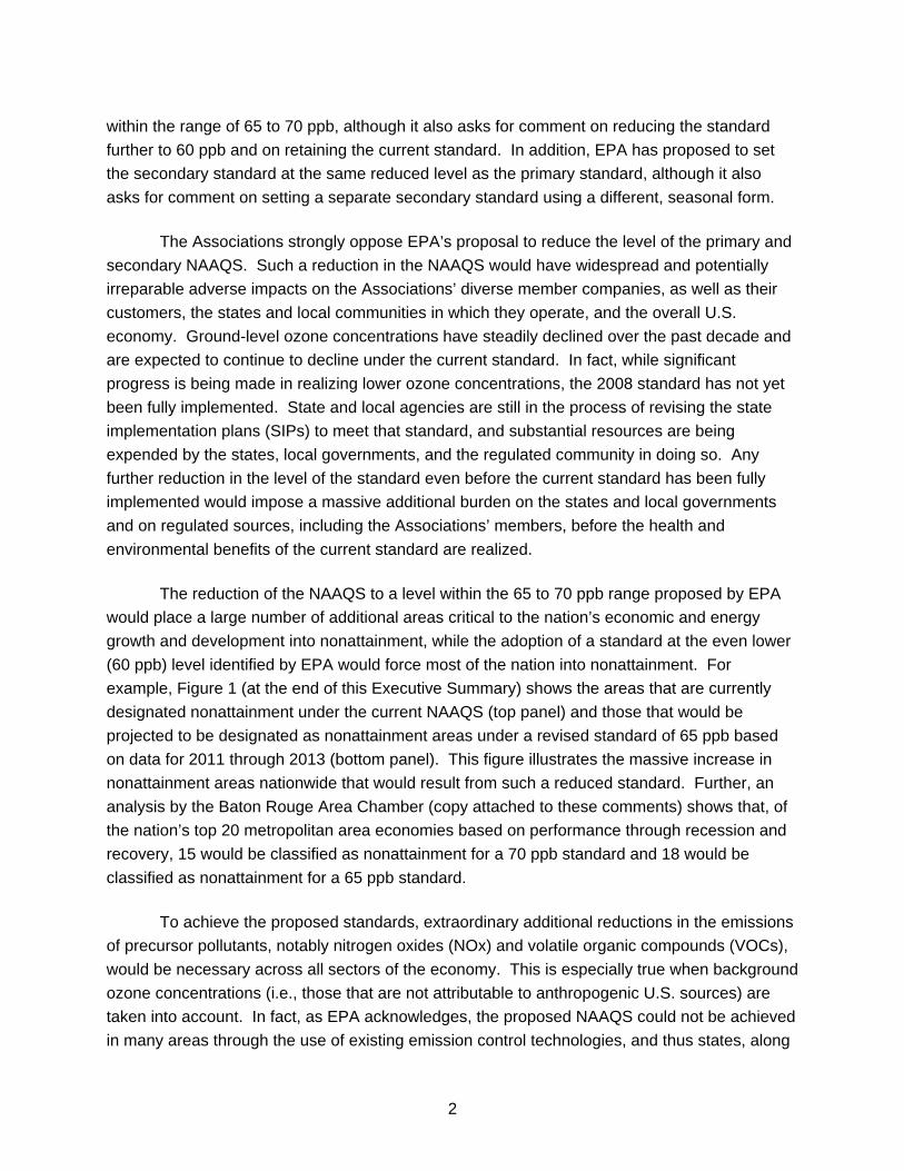
example, Figure 1 (at the end of this Executive Summary) shows the areas that are currently

designated nonattainment under the current NAAQS (top panel) and those that would be

projected to be designated as nonattainment areas under a revised standard of 65 ppb based

on data for 2011 through 2013 (bottom panel). This figure illustrates the massive increase in

nonattainment areas nationwide that would result from such a reduced standard. Further, an

analysis by the Baton Rouge Area Chamber (copy attached to these comments) shows that, of

the nation’s top 20 metropolitan area economies based on performance through recession and

recovery, 15 would be classified as nonattainment for a 70 ppb standard and 18 would be

classified as nonattainment for a 65 ppb standard.

To achieve the proposed standards, extraordinary additional reductions in the emissions

of precursor pollutants, notably nitrogen oxides (NOx) and volatile organic compounds (VOCs),

would be necessary across all sectors of the economy. This is especially true when background

ozone concentrations (i.e., those that are not attributable to anthropogenic U.S. sources) are

taken into account. In fact, as EPA acknowledges, the proposed NAAQS could not be achieved

in many areas through the use of existing emission control technologies, and thus states, along

3

with regulated sources, would have to rely on controls that are not even known at this time and

whose availability and costs cannot be reliably predicted. Indeed, it is likely that more than 60

percent of the necessary emissions reductions would need to come from such unknown

controls, and that such controls could be responsible for the great majority of the compliance

costs. Moreover, the impacts of the revised standards would be particularly severe in the

expanded nonattainment areas, where any new and modified sources would be subject to

additional costly and stringent permitting requirements under the nonattainment new source

review (NNSR) program, with the result that businesses may not be able to locate new

operations or grow existing operations in such areas. In addition, the proposed reduction in the

NAAQS would adversely affect local communities and the economy by potentially raising prices

for the goods and services produced by the Associations’ members and negatively impacting

economic growth. For example, in a recent analysis (copy attached to these comments), NERA

Economic Consulting (NERA) estimates that a standard of 65 ppb could have a present-value

cost of nearly $1.1 trillion based on costs over the period from 2017 through 2040, reduce the

U.S. Gross Domestic Product (GDP) by an average of about $140 billion per year or a total of

about $1.7 trillion over that period, result in a loss of approximately 1.4 million job equivalents,

and reduce the average U.S. household consumption by about $830 per year over the same

period. This could make such a revised ozone NAAQS the most expensive regulation ever

issued by the U.S. government.

As demonstrated in the Associations’ comments, this proposed revision of the NAAQS is

arbitrary, capricious, and unlawful under applicable legal standards for several reasons:

• EPA’s statement that its selection of a primary standard level that is requisite to protect

the public health with an adequate margin of safety is a “policy choice” left to “the

Administrator’s judgment” (79 Fed. Reg. at 75238) does not insulate its decision from

scrutiny. The Agency must still provide a reasoned explanation for its decision,

demonstrate that its decision comports with applicable legal requirements, and give

reasonable consideration to contextual factors affecting its policy decision. For the

reasons discussed below, EPA has not done so here.

• In proposing to lower the level of the standard, EPA has failed to take into account the

impact of background concentrations of ozone on the attainability of the standard –

specifically, the fact that such background levels could prevent attainment of the

proposed standard in large parts of the country. In this regard, EPA’s proposal fails to

take into account an important relevant factor under the Act, as required by fundamental

principles of administrative law; and it contravenes the Act’s requirement that NAAQS be

set at levels than can be achieved through regulation via SIPs (or plans issued by EPA if

states fail to adopt approvable SIPs). EPA’s description of potential regulatory

mechanisms to provide relief from nonattainment due to background concentrations is

4

no substitute for complying with the law; and in any case, those mechanisms are wholly

inadequate.

• EPA’s proposal is based primarily on a change in its interpretation of the scientific

evidence (e.g., the levels of risk that are judged acceptable), rather than any

fundamental change in the scientific understanding of ozone effects, since the Agency’s

last round of standard-setting in 2008. EPA has failed to provide a reasoned explanation

or justification for that change in judgment, as required by law.

• Given the limitations and uncertainties in the scientific data regarding the effects of

ozone exposure on human health and welfare at levels below the current standard (as

recognized by EPA and pointed out by other commenters), it would be arbitrary for EPA

to reduce the level of the current standard when that standard has not yet been fully

implemented.

• While the Act does not allow EPA to consider compliance costs when establishing or

revising NAAQS, it does not require EPA to eliminate all risks at any economic cost, and

it allows EPA to consider contextual factors, including the acceptability of the risks, in

determining the level “requisite” to protect public health and welfare. Given the

acknowledged uncertainties regarding the risks of ozone exposure at levels below the

current standard and regarding the incremental benefits that may accrue from lowering

that standard (especially in light of background concentrations), such a contextual

assessment should include consideration of the adverse social, economic, and energy

impacts from lowering the standard. EPA has failed to take such impacts into account,

and that failure would render its decision arbitrary and capricious.

• EPA’s proposal is also arbitrary and capricious because the Agency has not provided an

adequate justification for reducing the level of the primary standard. The Act requires

that NAAQS be set at a level that is sufficient, but not more stringent than necessary, to

protect public health and welfare. Given this requirement, and considering the above-

mentioned uncertainties and limitations in the evidence regarding the occurrence of

adverse health effects at levels below the current standard and the other relevant factors

discussed above (e.g., background concentrations, the attainability of a reduced

standard, the fact that the current standard has not been fully implemented, and the

adverse impacts of a reduced standard), the record does not support lowering the

current primary standard.

• Similarly, EPA has not provided an adequate justification for reducing the level of the

secondary standard given the significant uncertainties and limitations in the available

data on welfare effects at these low levels, as recognized by EPA and others. By

5

contrast, however, EPA has provided an adequate justification to retain the form of the

current secondary standard, rather than adopting a standard using the untested W126

form.

In addition to the forgoing points, these comments, supported by analyses conducted by

NERA (copies attached), show that EPA’s Regulatory Impact Analysis (RIA) for its proposal

significantly underestimates the costs of revising the ozone NAAQS through a series of faulty

assumptions, and at the same time overstates the asserted benefits attributable to such a

reduction in the ozone standard.

Finally, in these comments, the Associations address seven other issues raised by

EPA’s proposal. Specifically, they show that:

• EPA should allow the flagging and documenting of “exceptional events” causing

exceedances of the NAAQS at any time prior to an attainment decision or, at a

minimum, should extend the time for flagging and documenting such events as it has

proposed;

• EPA’s proposal to “grandfather” certain pending applications for Prevention of Significant

Deterioration (PSD) permits, if finalized, could provide limited relief from the immediate

burden imposed on certain PSD permit applicants by a revised NAAQS, but provides no

workable solution to the broader problem for building or expanding the types of sources

that fuel economic growth;

• If EPA finalizes revisions to the NAAQS, it should provide states with the necessary

implementation guidance and regulations at the time of promulgating the revised

NAAQS and give states as much time as possible to implement the revised NAAQS;

• Even if EPA finalizes revisions to the NAAQS, it should not revise its Air Quality Index

because such a revision is not required and would produce misleading information for

the public;

• EPA should not extend the ozone monitoring season, as it has proposed for 33 states;

• EPA’s proposal does not comply with the federal Information Quality Act; and

• EPA has not complied with the Unfunded Mandates Reform Act in its proposal.

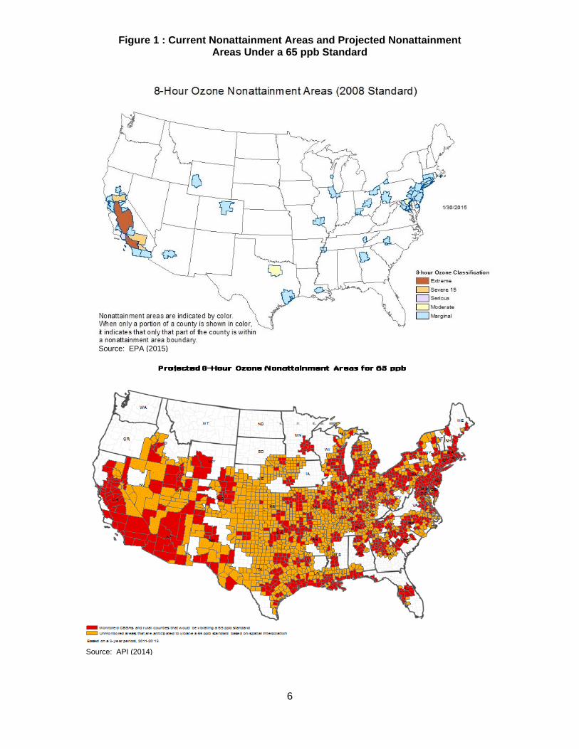
Figure 1 : Current Nonattainment Areas and Projected Nonattainment Areas Under a 65 ppb Standard

6

Source: EPA (2015)

Source: API (2014)

7

II. BACKGROUND INFORMATION

A. Legal Requirements

Section 108 of the Act directs EPA to set NAAQS for pollutants “the emissions of which .

. . cause or contribute to air pollution which may reasonably be anticipated to endanger public

health or welfare” (§ 108(a)(1)(A)).1 The NAAQS must be based on “air quality criteria . . . [that]

accurately reflect the latest scientific knowledge useful in indicating the kind and extent of all

identifiable effects on public health or welfare” (§ 108(a)(2)). Section 109 of the Act further

provides that EPA must review NAAQS at least every five years and revise them “as may be

appropriate” in accordance with Sections 108 and 109(b) of the Act (§ 109(d)(1)). Primary

NAAQS must be set at a level “requisite to protect the public health” with “an adequate margin

of safety” (§ 109(b)(1)). Secondary NAAQS must specify a level of air quality “requisite to

protect the public welfare from any known or anticipated adverse effects” (§ 109(b)(2)).

NAAQS are not intended to eliminate all risk. As the Supreme Court has explained,

“requisite to protect” means “not lower or higher than is necessary.” Whitman v. American

Trucking Ass’ns, 531 U.S. 457, 476 (2001). Thus, in setting NAAQS, EPA must determine the

levels of a pollutant that are “sufficient, but not more than necessary” to protect the public health

and welfare. Id. at 473 (internal quotation marks omitted). This requires an assessment of the

extent to which the risks from exposure to the pollutant are unacceptable; and that assessment,

in turn, requires EPA to take into account background considerations and context. As noted by

Justice Breyer in Whitman, Section 109 “does not require the EPA to eliminate every health risk,

however slight, at any economic cost, however great.” Id. at 494 (Breyer, J., concurring in part

and concurring in the judgment). Instead, it allows the EPA Administrator, in determining the

levels “requisite” to protect the public health, to consider various contextual factors, including:

“background considerations, such as the public’s ordinary tolerance of the particular health risk

in the particular context at issue”; “the severity of a pollutant’s potential adverse health effects,

the number of those likely to be affected, the distribution of the adverse effects, and the

uncertainties surrounding each estimate”; “comparative health consequences”; and “the

acceptability of small risks to health.” Id. at 494-95. The D.C. Circuit recently confirmed that

setting primary NAAQS may require such a contextual assessment as described by Justice

Breyer. Mississippi v. EPA, 744 F.3d 1334, 1343 (D.C. Cir. 2013).

In addition, the legislative history of Section 109 makes clear that Congress intended the

primary NAAQS to be set at a level requisite to protect sensitive subpopulations but not the

most sensitive individuals within those subpopulations. See S. Rep. No. 91-1196 at 10 (1970).

As stated in that report, in establishing NAAQS that will protect the health of sensitive

1 For ease of reference, these comments cite directly to sections of the Clean Air Act; parallel citations to the U.S. Code (42 U.S.C. § 7401 et seq.) are not included.

8

populations, “reference should be made to a representative sample of persons comprising the

subgroup rather than to a single person in such group.” Id. EPA and the courts have

consistently recognized that the NAAQS are not required to protect the most sensitive

individuals within a population.2

With respect to the secondary standard, the Act does not require a secondary standard

that differs from the primary standard. A secondary standard may be the same as the primary

standard so long as the level specified is shown to be “requisite to protect the public welfare

from any known or anticipated adverse effects” (§ 109(b)(2)). See American Farm Bureau

Federation v. EPA, 559 F.3d 512, 530 (D.C. Cir. 2009); Mississippi, 744 F.3d at 1358. In fact,

EPA has established secondary NAAQS that are the same as primary NAAQS for several

pollutants.3

Consistent with the recognition that NAAQS are not intended to result in zero risk and

may take into account contextual factors such as the public’s tolerance of acceptable risks,

NAAQS are not intended to reduce pollutant concentrations to or below background levels – i.e.,

levels that would exist in the absence of anthropogenic emissions that are subject to regulation

under the Act. Rather, NAAQS are to be standards that can be attained by regulation of U.S.

sources. This is demonstrated by the requirement in Section 107(a) that SIPs are to specify the

manner in which the NAAQS “will be achieved and maintained,” as well as the requirement of

Section 110(a)(2)(C) that SIPs must include an enforcement and regulation program “as

necessary to assure that [NAAQS] are achieved” (emphases added). These provisions

demonstrate Congress’s intention that NAAQS are to consist of standards that can be achieved

through SIPs, which would not be the case if such attainment is prevented by emissions that are

not subject to regulation under the SIPs.

The CAA also specifies the role of the Clean Air Scientific Advisory Committee

(CASAC). It provides that, at five-year intervals, CASAC shall review the EPA-prepared air

quality criteria and the primary and secondary NAAQS and shall recommend to the

Administrator any new NAAQS or revisions of existing criteria and NAAQS as may be

appropriate (§ 109(d)(2)(B)). The Act provides further that, if a NAAQS proposal by EPA “differs

2 See 75 Fed. Reg. 6474, 5475 n.2 (Feb. 9, 2010) (primary NAAQS for nitrogen dioxide); 71 Fed. Reg. 61144, 61145 n.1 (Oct. 17, 2006) (NAAQS for particulate matter); 50 Fed. Reg. 37484, 37488 (Sept. 13, 1985) (NAAQS for carbon monoxide), 44 Fed. Reg. 8202, 8210 (Feb. 8, 1979) (NAAQS for photochemical oxidants); see also Lead Industries Ass’n v. EPA, 647 F.2d 1130 (D.C. Cir. 1980) (upholding EPA’s establishment of the initial NAAQS for lead at a level that it estimated would protect 99.5% of the sensitive population from “potentially adverse” effects); Safe Air for Everyone v. Idaho, 469 F. Supp. 2d 884, 892 (D. Idaho 2006) (recognizing that the NAAQS “are designed to protect sensitive populations but not required to protect the most sensitive within a population”). 3 See, e.g., 24-hour NAAQS for particulate matter with a mean diameter less than 10 micrometers (PM10) (40 C.F.R § 50.6); annual NAAQS for nitrogen oxides (NOx) (id. § 50.11); NAAQS for lead (id. § 50.12).

9

in any important respect” from CASAC’s recommendations, EPA must provide “an explanation

of the reasons for such differences” (§ 307(d)(3)). The D.C. Circuit has reiterated that

requirement (see American Farm Bureau, 559 F.3d at 521); but it has also made clear that,

since the setting of NAAQS is ultimately the EPA Administrator’s decision, the Administrator

may depart from CASAC’s recommendations so long as an explanation is provided, and that

even the requirement to provide a scientific explanation for disagreeing with CASAC applies

only to CASAC’s recommendations on scientific issues, not to its recommendations based on

policy judgments, which are entitled to a lesser degree of deference. Mississippi, 744 F.3d at

1355-58. Further, in addition to providing advice on NAAQS, CASAC is charged with advising

EPA on various other matters, including “the relative contribution to air pollution concentrations

of natural as well as anthropogenic activity” and “any adverse public health, welfare, social,

economic, or energy effects which may result from various strategies for attainment and

maintenance” of the NAAQS (CAA § 109(d)(2)(C)).

B. Historical Context

1. 1997 NAAQS

In 1997, EPA revised the primary NAAQS for ozone from a one-hour average standard

of 0.12 parts per million (ppm) (with one allowable exceedance per year) to an 8-hour standard

of 0.08 ppm, based on the annual 4th highest daily maximum 8-hour average concentration over

a three-year period. 62 Fed. Reg. 38856 (July 18, 1997). In doing so, EPA concluded that

“[t]he 8-hour averaging time is more directly associated with health effects of concern at lower

O3 concentrations than is the 1-hour averaging time,” and that “an 8-hour standard would limit

both 1- and 8-hour exposures” (id. at 38861). With regard to the level of the standard, EPA first

acknowledged that, as increasingly stringent standards were evaluated, including an 8-hour

standard of 0.07 ppm, the estimated risks decreased for respiratory functional and symptomatic

effects and for hospital admissions for respiratory causes (id. at 38864). EPA also

acknowledged that there might be no ozone level “below which absolutely no effects are likely to

occur” (id. at 38863). Nevertheless, EPA determined that a standard more stringent than 0.08

ppm was “not requisite to protect the public health with an adequate margin of safety” (id. at

38868). In support of this determination, EPA noted, among other things, that “there is no . . .

bright line that differentiates between acceptable and unacceptable risks within [the] range” of

0.07 to 0.09 ppm (id. at 38864), and that a standard of 0.07 ppm “would be closer to peak

background levels that infrequently occur in some areas due to nonanthropogenic sources of

[ozone] precursors” (id. at 38868).

With respect to the secondary standard, EPA recognized in 1997 that it had

considerable evidence on the effects of ozone on vegetation. It also acknowledged that “the

available scientific information supports the conclusion that a cumulative seasonal exposure

index . . . is more biologically relevant than a single event or mean index” (id. at 38875).

10

Nevertheless, the Administrator chose to set the secondary standard equal to the new 8-hour

primary standard (id. at 38877). Specifically, the Administrator decided not to set a seasonal

secondary standard due to the “substantial uncertainties” as to whether increased welfare

protection would result from such a standard (id. at 38877-78).

The primary and secondary NAAQS promulgated in 1997 were challenged in court as

both overly stringent and not stringent enough, but were ultimately upheld against those

challenges. See American Trucking Ass’ns v. EPA, 283 F.3d 355, 378-80 (D.C. Cir. 2002),

upon remand from 531 U.S. 457 (2001). In rejecting the challenge that the standard was not

stringent enough, the D.C. Circuit held that EPA had engaged in reasoned decision-making in

selecting a level of 0.08 ppm rather than 0.07 ppm. In reaching this conclusion, the court

referred to EPA’s determination that a standard of 0.07 ppm was too close to background, and it

stated that, “although relative proximity to peak background ozone concentrations did not, in

itself, necessitate a level of 0.08, EPA could consider that factor when choosing among three

alternative levels” (283 F.3d at 379).

2. 2008 NAAQS

Following an extensive review, EPA issued revised primary and secondary NAAQS for

ozone in 2008. 73 Fed. Reg. 16436 (March 27, 2008). In that rulemaking, EPA revised the

primary standard to a level of 0.075 ppm (75 ppb), concluding that the prior standard was not

requisite to protect the public health. In reaching that conclusion, EPA relied in particular on

controlled human exposure (clinical) studies, which it said showed consistent evidence of

respiratory effects (lung function decrements and respiratory symptoms) in healthy subjects at

ozone levels of 80 ppb and above, along with two new such studies (Adams, 2002, 2006)

showing such effects in some subjects at lower levels (specifically, 60 ppb), as well as an EPA

statistical re-analysis of the data from one of those studies indicating that the effects shown at

60 ppb were statistically significant (see, e.g., 73 Fed. Reg. at 16445, 16454-55, 16476, 16478).

In addition, EPA relied on information indicating that people with asthma or other lung disease

are likely to experience larger and more serious effects than healthy people (e.g., id. at 16445,

16470, 16471, 16476). Further, EPA asserted that there was new epidemiological evidence

showing significant associations of ozone exposure with a wide range of health effects,

including respiratory emergency room visits and hospital admissions and premature mortality, at

ozone levels at and below 80 ppb (e.g., id. at 16446, 16471, 16476).

At the same time, although CASAC had recommended setting the primary standard in

the range of 60 to 70 ppb, EPA determined that the data did not warrant adoption of such a

lower standard due to the “limited” human clinical evidence of effects at lower levels and the

uncertainties in the epidemiological studies regarding causal relationships between the effects

reported and ozone exposures at levels below the then-current standard (e.g., id. at 16476,

16479). Overall, EPA reached the following conclusion:

11

“Taking into account the uncertainties that remain in interpreting the evidence from

available controlled human exposure and epidemiological studies at very low levels,

the Administrator notes that the likelihood of obtaining benefits to public health with a

standard set below 0.075 ppm O3 decreases, while the likelihood of requiring

reductions that go beyond those that are needed to protect public health increases. .

. . The Administrator believes that a standard set at 0.075 ppm would be sufficient to

protect public health with an adequate margin of safety, and does not believe that a

lower standard is needed to provide this degree of protection.” (Id. at 16483.)

EPA also revised the secondary standard for ozone to be the same as the primary

standard. Taking into account CASAC’s views and findings from the previous ozone NAAQS

review, EPA concluded that a cumulative, seasonal standard, such as the “W126” sigmoidally

weighted index, was the most “biologically relevant way to relate [ozone] exposure to plant

growth response” (id. at 16500). Nevertheless, based on an analysis comparing the protection

that would be afforded by revised primary NAAQS and the top of the range (21 ppm-hours) of

proposed levels under consideration as a W126 standard, EPA determined that adopting a

cumulative, seasonal standard was unnecessary due to the “significant overlap between the

revised 8-hour primary standard and selected levels of the [W126] standard form being

considered” (id.). Acknowledging that an 8-hour standard might not provide the “appropriate

degree of protection” for vegetation in some areas, EPA nonetheless determined that

establishing a W126 standard “would result in uncertain benefits beyond those provided by the

revised primary standard” and was therefore unnecessary (id.). Accordingly, EPA decided to

revise the existing 8-hour secondary standard by making it identical to the revised primary

standard (id.).

3. EPA’s 2010 Reconsideration and Withdrawal

In January 2010, EPA issued a notice of proposed rulemaking to reconsider the 2008

NAAQS. 75 Fed. Reg. 2938 (Jan. 19, 2010). In that notice, EPA proposed to reduce the level

of the primary standard from 75 ppb to a level in the range of 60 to 70 ppb, and to establish a

new secondary standard using a seasonal form. After receiving comments from the public and

CASAC on that proposal, EPA ultimately withdrew that reconsideration proceeding and

consolidated it with the Agency’s next statutory review.

4. D.C. Circuit’s Decision on 2008 NAAQS

In July 2011, the D.C. Circuit issued a decision ruling on several challenges to the 2008

NAAQS in the Mississippi case. The court upheld the 2008 primary standard of 75 ppb against

both arguments that it was overly stringent and arguments that it was not stringent enough. The

court held that EPA reasonably determined that the previous standard of 0.08 ppm (which

rounded to 84 ppb) needed to be reduced given “numerous epidemiological studies linking

12

health effects to exposure to ozone levels below 0.08 ppm and clinical human exposure studies

finding a causal relationship between health effects and exposure to ozone levels at and below

0.08 ppm” (744 F.3d at 1345). At the same time, the court held that EPA was not required to

reduce the standard below 75 ppb (0.075 ppm). In so holding, the court relied on EPA’s

determination that the new human clinical evidence from the Adams studies was “too limited” to

support a reduction to 60 ppb (0.06 ppm) (id. at 1350). It stated: “The Adams results at 0.06

ppm indicate some degree of risk that some number of individuals might continue to experience

health effects at and below 0.075 ppm, but we have previously acknowledged the impossibility

of eliminating all risk of health effects from ‘non-threshold’ pollutants like ozone” (id. at 1350-51).

Further, the court explained that EPA reasonably relied on the limitations and uncertainties in

the epidemiological studies with respect to whether the effects reported could be attributed to

ozone levels below 75 ppb (id. at 1351-52). Additionally, the court found that EPA was not

required to provide a scientific explanation for departing from CASAC’s recommendations since

CASAC did not make clear whether its recommendations were based on science rather than

policy (id. at 1356-58).

The court remanded the secondary standard to EPA, holding that the Agency had not

satisfied the CAA’s requirements because EPA had not identified the level of protection that was

“requisite to protect the public welfare” (id. at 1359). The court concluded that “it is insufficient

for EPA merely to compare the level of protection afforded by the primary standard to possible

secondary standards and find the two roughly equivalent” (id. at 1360-61). Instead, EPA was

obligated to expressly determine the requisite level of protection and provide a rationale for that

determination (id. at 1361). Further, the court found that EPA’s comparison between the

revised 8-hour standard and a seasonal standard was insufficient to treat one as a surrogate for

the other because “EPA failed to explain why it looked only at one potential seasonal standard

that the primary standard would arguably protect as well as” (id.).

5. EPA’s Review of Post-2008 Information and Comments to EPA and CASAC

During the latest review cycle (which had begun during the reconsideration discussed

above), EPA staff prepared a variety of documents to inform its decision on revising the

NAAQS. These documents included the Integrated Science Assessment (ISA) (EPA, 2013), the

Health Risk and Exposure Assessment (HREA) (EPA, 2014a), the Welfare Risk and Exposure

Assessment (WREA) (EPA, 2014b), and the Policy Assessment (PA) (EPA, 2014c). Drafts of

these documents were subject to review by CASAC and the public, and the documents were

finalized following those reviews.

Health Effects Evidence. In discussing controlled human exposure studies, the EPA staff

documents relied in particular on two new studies that had been published since 2008 (see ISA

at 6-11 – 6-20; PA at 3-56 – 3-59). The first was a study by Schelegle et al. (2009), who

reported the responses of 31 healthy subjects, during and after periods of exercise, with 6.6-

13

hour inhalation exposure to mean ozone levels of 88, 81, 72, and 63 ppb.4 These investigators

reported that, at the 72 ppb exposure level, the subjects had a statistically significant decrease

in lung function (mean decrease of approximately 5% in forced expiratory volume in one second

[FEV1]) and an increase in subjective symptoms (mean score of approximately 13 on a severity

scale of 0 to 40), but that there were no statistically significant effects at 60 ppb. The second

new study was a study by Kim et al. (2011), who investigated the effects of 6.6-hour exposure to

60 ppb ozone on 59 healthy exercising subjects. These investigators found small but

statistically significant changes in lung function and inflammatory markers, but no increase in

respiratory symptoms. Additionally, EPA staff referred to exposure models based on these

studies along with the prior Adams (2002, 2006) studies (see ISA at 6-17 – 6-18).

Comments on the EPA staff documents provided to CASAC explained that these new

studies did not fundamentally alter the understanding of the respiratory effects of ozone based

on the human clinical data, compared to the information available during the previous ozone

NAAQS review. As they indicated, the previous studies, particularly those of Adams (2002,

2006), showed that these types of responses occur at ozone levels at and above 80 ppb and

decrease in size and severity and in the number of individuals affected at levels down to 60 ppb,

and the new studies simply confirm those conclusions. For example, comments by Jon Heuss

and George Wolff to CASAC explained that “[r]ecent human clinical studies do not change what

was known about ozone effects in the last review” (Heuss and Wolff, 2012, at 12), and that

“[a]though there are now more studies of 6- to 8-hour exposures to low ozone concentrations

while exercising heavily, EPA’s estimate of the dose-response curve at low concentrations has

not changed appreciably” (Heuss et al., 2014, at 10). No new clinical studies on the effects of

ozone exposure on asthmatics or other “at-risk” individuals were identified.

The EPA staff documents also discussed the epidemiological studies that had become

available since the prior review, concluding that those more recent studies largely support and

strengthen EPA’s prior conclusions regarding a likely causal association between ozone

exposure and respiratory effects (see, e.g., ISA at 6-152, 6-165, 6-261). However, commenters

demonstrated that those newer studies are subject to the same uncertainties as the prior

studies regarding the ability to attribute the effects to ozone exposure, particularly at levels

below the current standard (see, e.g., Gradient, 2013a,b,c; Heuss and Wolff, 2012 at 19-27).

Overall, during the course of these reviews, substantial comments were submitted to

EPA and CASAC pointing out the limitations and uncertainties of the available health effects

information on the relevant issues, including: (a) the statistical and health significance of the

lung function and symptomatic responses reported in human clinical studies at ozone levels

below the current standard of 75 ppb; (b) the evidence regarding larger or more serious effects

4 The target ozone levels in this study were 87, 80, 70, and 60 ppb, respectively, but those listed in the text were the actual mean ozone exposure levels during the study,

14

in asthmatics and other “at-risk” individuals; (c) the consistency of the epidemiological studies

and their ability to reliably attribute the morbidity and mortality effects reported to ozone levels at

and below the current standard; (d) the reliability of EPA’s exposure and risk analyses in the

HREA for estimating risks to the U.S. population; and (e) potential benefits of a revised standard

in preventing those risks (see, e.g., Goodman and Sax, 2014a,b; Goodman et al., 2013a;

American Chemistry Council et al., 2014; Gradient, 2013a,b,c; Heuss and Wolff, 2012; Heuss et

al., 2014).

Welfare Effects Evidence. With respect to the secondary standard, the ISA identified

new studies that EPA said enhanced its understanding of ozone welfare effects. For instance,

the ISA identified a 2009 meta-analysis, Wittig et al. (2009), as providing important new

information on ozone impacts on root biomass and root:shoot ratio (ISA at 9-42 to 9-45).

Comments on the ISA, however, pointed out that Wittig et al. relied on studies that made use of

highly unreliable models to establish pre-industrial ozone concentrations (see UARG, 2012, at

7). The ISA also addressed new scientific information related to crop yield loss (ISA at 9-57 to

9-67), although commenters pointed out that there is no information on how to account for

agricultural management and competing agricultural policies in devising a secondary NAAQS to

address this welfare effect (UARG, 2012, at 9). In addition, the ISA reviewed new research

addressing broader ecosystem effects of ozone but acknowledged that most of the new studies

merely confirmed what was already known at the time of the previous review (ISA at 9-67 to 9-

98). The ISA did place significant emphasis on a study by Grulke et al. (2008) linking ozone

concentrations and increased forest susceptibility to wildfire (ISA at 9-88). Commenters pointed

out, however, that Grulke et al. (2008) did not show a statistical correlation between ozone and

wildfires and that numerous confounders, such as drought and insect infestations, were not

controlled for (UARG, 2012, at 8).

EPA’s WREA included several quantitative analyses related to the key welfare effects

that EPA chose to evaluate. With respect to relative biomass loss (RBL) in trees, a key effect in

this review of the secondary standard, EPA calculated exposure-response functions based on

seedling RBL values and then extrapolated those values to RBL estimates for mature trees

(WREA at 6-4 to 6-6). Commenters on the WREA explained that the exposure-response

functions were highly uncertain due to limitations in EPA’s W126 estimates, both because of the

limited number of tree species studied and because of problems inherent in extrapolating effects

from seedlings to trees at other developmental stages (Gradient, 2014, at 7, 13-16). The WREA

also included a national scale assessment for tree RBL using a 2% RBL benchmark

recommended by CASAC (WREA at 7-19 to 7-34). Commenters explained, however, that there

was no justification for the 2% benchmark (Gradient, 2014, at 16).

The WREA included additional analyses related to visible foliar injury effects of ozone,

including a screening assessment of impacts at 214 national parks and a case study

15

assessment of three national parks in an attempt to quantify the value of mitigating foliar injury

(WREA at 7-34 to 7-58). Comments on these analyses pointed out that the screening-level

assessment had significant uncertainties because none of the available studies linking ozone

exposures to foliar injury used or reported the W126 metric (Gradient, 2014, at 10). With

respect to the case studies, EPA itself acknowledged that it was unable to quantify “the

monetary value of the [relevant] services given the data and methodology limitations inherent in

such an effort” (WREA at 7-34).

In the PA, EPA staff concluded that there was a basis for finding the current secondary

standard inadequate and recommended that the Administrator consider revising the secondary

ozone standard to a W126 form set at a level ranging from 17 ppm-hrs to 7 ppm-hrs (PA at 6-57

to 6-58). In addition to addressing scientific issues, comments on the PA explained that the PA

did not provide an adequate basis for determining that the observed or projected welfare

impacts were adverse (UARG, 2014, at 43-44). Commenters also noted that the record

supported a finding that the current 75 ppb secondary standard would provide welfare protection

consistent with the range of W126 values that the staff recommended for consideration

(Gradient, 2014, at 3-6).

Background Ozone Concentrations. In addition to the forgoing issues, the EPA staff

documents contained discussions of “background” ozone concentrations and various ways to

account for such background. In its prior review in 2007, EPA introduced the term Policy

Relevant Background (PRB), which was defined as ozone concentrations in the U.S. in the

absence of anthropogenic emissions of precursor pollutants – i.e., volatile organic compounds

(VOCs), nitrogen oxides (NOx), methane (CH4), and carbon monoxide (CO) – from sources in

the U.S., Canada, and Mexico; and it attempted to model such concentrations. In initial drafts of

the ISA, the EPA staff continued to follow that approach, based on the erroneous assumption

that emissions from sources in Canada and Mexico could be controlled by treaties or

international agreements for purposes of NAAQS implementation. In the final ISA and PA, EPA

included three definitions of background: (1) natural background, consisting of concentrations

that would exist in the absence of any anthropogenic emissions of precursor pollutants; (2)

North American background, consisting of concentrations that would exist in the absence of

anthropogenic precursor emissions from North America; and (3) U.S. background (USB),

consisting of concentrations that would exist in the absence of anthropogenic emissions from

sources in the U.S. For the reasons discussed above, only USB constitutes true background for

purposes of evaluating the implications for setting NAAQS, since only U.S. sources are subject

to regulation under the SIPs. However, during the reviews of the EPA staff documents, several

commenters pointed out that EPA had still not adequately determined USB, was

underestimating USB concentrations, and was still not properly taking into account the impact of

USB on projected attainment of the ozone NAAQS (see, e.g., Wolff et al., 2014; Lefohn and

16

Oltmans, 2012, 2014 [the latter showing that a large percentage of the risks calculated by EPA

is associated with ozone concentrations in the background range]; Kaiser, 2014).

Other Issues. Finally, in the course of these reviews, many of the Associations urged

CASAC to comply with its statutory obligation to provide advice to EPA on any adverse social,

economic, and energy effects from efforts to attain revised ozone NAAQS, as required by CAA

§ 109(d)(2)(C) (see, e.g., Air-Conditioning, Heating, and Refrigeration Institute et al., 2014).

However, CASAC did not do so.

C. EPA’s Proposed Rule

In its December 2014 proposal, EPA proposes to retain the indicator, averaging time,

and form of the current 8-hour primary standard, but to reduce the level of the standard to a

level within the range of 65 to 70 ppb, although it also asks for comment on reducing the

standard further to 60 ppb and on the option of retaining the current standard of 75 ppb (79 Fed.

Reg. 75234, 75236). In addition, EPA proposes to reduce the level of the secondary standard

by making it the same as the revised primary standard, although it also asks for comment on

setting a separate secondary standard using the seasonal W126 form (id. at 75237). In its

proposal, EPA itself acknowledges the uncertainties in the interpretation of the scientific data, as

discussed below.

1. Statements on Level of Primary Standard

To support the proposed change in the level of the primary standard, EPA relies most

heavily on the controlled human exposure studies which it says showed adverse respiratory

effects in healthy subjects at ozone levels “as low as 72 ppb” (id. at 75288, 75288-89, 75291,

75304). Specifically, EPA relies on the Schelegle et al. (2009) study, discussed above, which

reported a statistically significant group mean decrease in FEV1 and an increase in subjective

symptoms at the 72 ppb exposure level. EPA asserts in several places that the responses

observed in the Schelegle et al. study meet the criteria for adverse health effects (id. at 75288,

75289, 75304). However, these assertions must be referring to responses of individual study

subjects, since EPA does not claim that transitory FEV1 decrements less than 10% (such as the

mean change of ~ 5% identified in this study) are adverse. Indeed, only six of the 31 subjects in

this study exhibited an FEV1 decrement equal to or greater than 10%. Moreover, in this study,

individuals that exhibited FEV1 decrements in response to 72 ppb ozone were not always the

same individuals that reported the respiratory symptoms, making the results of this study

confusing at best. Further, the Agency states that, for healthy people, including children, FEV1

decrements between 10% and 20% and/or moderate symptomatic responses “would likely

interfere with normal activity for relatively few sensitive individuals” (id. at 75263).

17

EPA also continues to assert, as it did in 2008, that “at-risk” individuals, such as children

and people with asthma, could experience larger and/or more serious effects at the same levels

(id., 75263, 75280, 75288). However, it recognizes that there are no direct data to support that

claim since “the controlled human exposure studies that provided the basis for health

benchmark comparisons have not evaluated at-risk populations” (id. at 75273).

EPA further relies on single-city epidemiological studies that reported associations of

ozone with respiratory effects in cities where EPA believes that the current standard would have

been met (id. at 75289, 75291, 75307). In particular, it cites a study in Seattle by Mar and

Koenig (2009), who reported associations of ozone levels with respiratory emergency

department visits for asthma in a location that EPA says would likely have met the current

standard of 75 ppb but would not have met a standard of 70 ppm (id. at 75280, 75289, 75307).

At the same time, EPA recognizes that epidemiological studies are subject to a general

uncertainty in determining “the extent to which reported health effects are caused by exposures

to O3 itself, as opposed to other factors such as co-occurring pollutants or pollutant mixtures,”

and that “this uncertainty becomes an increasingly important consideration as health effect

associations are evaluated at lower ambient O3 concentrations” (id. at 75282). Further, EPA

notes specifically that the extent to which the reported ozone-associated emergency department

visits in the Seattle study could have been reduced by a standard at or below 70 ppb is

uncertain (id. at 75307).

EPA places supporting, but less, weight on the multi-city epidemiological studies (id. at

75280-81, 75289, 75291, 75307-08). However, the Agency recognizes “important uncertainties”

in reliance on these studies – e.g., uncertainties stemming from the heterogeneity in effect

estimates among locations, uncertainties in linking multi-city effect estimates (aggregated

across multiple cities) to ozone levels below the current standard, uncertainties in identifying

concentration-response relationships, etc. (id. at 75282, 75307). EPA also acknowledges that

the long-term studies of respiratory effects, including mortality, were not conducted in locations

that would have met the current standard and have not reported concentration-response

relationships that indicate confidence in health effects associated with ozone concentrations

meeting the current standard (id. at 75282).

EPA relies further on the modeled risk estimates derived from its HREA (id. at 75289-

91). Again, the Agency relies primarily on risk estimates derived from the controlled human

exposure studies and gives less weight to risk estimates derived from epidemiological studies

due to substantial uncertainties about those estimates. Specifically, EPA recognizes numerous

“key uncertainties” in the epidemiologic-based risk estimates, including “the heterogeneity in

effect estimates between locations, the potential for exposure measurement errors, and the

uncertainty in the interpretation of the shape of the concentration-response functions for O3

concentrations in the lower portions of ambient distributions” (id. at 75289 & 75303; see also id.

18

at 75277-79). As an example of the last of these, EPA recognizes that “lower confidence”

should be placed in the HREA’s estimates of respiratory mortality from long-term ozone

exposure, which are based on a study by Jerrett et al. (2009), due to the uncertainties in that

study about the attribution of the effects to any particular concentration of ozone (id. at 75277,

75300). It should also be noted that EPA’s HREA evaluates exposures and risks from all

sources, including natural sources and non-U.S. anthropogenic sources as well as U.S.

anthropogenic sources, and thus does not characterize the exposures and risks that could be

addressed by a change in the NAAQS.

In its proposal, EPA rejects the need to set a primary standard at a level below 65 ppb.

In this regard, EPA notes that, at levels below 72 ppb, “the combination of statistically significant

increases in respiratory symptoms and decrements in lung function has not been reported,”

citing the findings of Adams (2006), Schelegle et al. (2009), and Kim et al. (2011) of no

statistically significant increases in symptoms at 60 and 63 ppb (id. at 75304). The proposal

thus states that “[t]he Administrator has decreasing confidence that adverse effects will occur

following exposures to O3 concentrations below 72 ppb” (id.). EPA states further that a standard

below 65 ppb would not be warranted “given the uncertainties associated with the adversity of

exposures to 60 ppb O3, particularly single occurrence of such exposures; uncertainties

associated with air quality analyses in locations of multicity epidemiologic studies; and

uncertainties in epidemiology-based risk estimates, particularly uncertainties in the shape of the

concentration-response functions at lower O3 concentrations and uncertainties associated with

the heterogeneity in O3 effect estimates across locations” (id. at 75309).

2. Statements on Secondary Standard

As stated above, EPA is proposing to revise the secondary ozone standard to be the

same as the revised primary standard. Its basis for this proposal is the proposed determination

that air quality providing exposures within the range of 13 ppm-hours to 17 ppm-hours would be

“requisite to protect the public welfare” and that an 8-hour standard set at the level of 70 ppb

would achieve such air quality. Accordingly, EPA’s proposed rule is composed of statements

made in support of its proposed W126 range of protective air quality and its assessment of

equivalency between that range of air quality and an 8-hour standard in a traditional NAAQS

form.

To support its proposed determination that a 13 ppm-hour to 17 ppm-hour range is

requisite to protect public welfare, EPA cites three categories of welfare effects: (1) impacts on

tree growth, productivity, and carbon storage; (2) crop yield loss; and (3) visible foliar injury (id.

at 75315). With respect to all three categories, the proposed rule acknowledges that the current

body of scientific evidence confirms prior conclusions and that no major scientific advances

have occurred that have altered fundamental knowledge with respect to these effects (79 Fed.

Reg. at 75314, 75316, 75317, 75319).

19

The proposed rule relies in particular on relative biomass loss (RBL) in trees to support

the proposed revision to the secondary NAAQS (id. at 75335). The exposure-response

functions developed from studies of 11 species of tree seedlings are the centerpiece of this area

of the science (id. at 75318). The proposed rule acknowledges key limitations in the exposure-

response functions – namely, that they are derived from a limited number of studies (and in

some cases only a single study) per species (id. at 75318), that effects on seedlings are not

equal to effects on mature trees (id. at 75339), and that they are based on studies of less than

0.8% of tree species in the United States and may not be representative of sensitivity in other

species (id. at 73256). The proposed rule also points to assessments in the WREA indicating

that, under the current secondary standard, only approximately 0.2% of the country would

experience 2% RBL; and it recognizes that another WREA study indicated that, in most counties

where a species experienced a 2% RBL during air quality conditions that meet the current

standard, that effect was found only for a single, sensitive species (id. at 75324). Most

importantly, in the proposed rule, EPA acknowledges that the 2% RBL benchmark it had

previously relied upon was actually based on “no explicit rationale” (id. at 75321); and it

proposes to conclude that a 6% RBL benchmark is a more reliable measure by which to judge

adverse RBL effects (id. at 75349).

The proposed rule also describes the science characterizing crop yield loss and visible

foliar injury. As to crop yield loss, however, EPA states that “agricultural crops do not have

same need for additional protection from the NAAQS as forested ecosystems and, while

research on agricultural crop species remains useful in illuminating mechanisms of action and

physiological processes, information from this sector on O3-induced effects is considered less

useful in informing judgments on what level(s) would be sufficient but not more than necessary

to protect the public welfare” (id. at 75348). With respect to visible foliar injury, the proposed

rule notes that there are likely to be only minimal effects at air quality levels meeting the current

secondary standard (id. at 75328), and that there is little scientific information and no guidance

from federal land managers to help make reliable determinations as to what constitutes adverse

visible foliar injury effects (id. at 75316, 75334). Accordingly, EPA places less emphasis on

these welfare effects in its proposed determination that a range of 13 ppm-hours to 17 ppm-

hours would be requisite to protect the public welfare.

The proposed rule relies on an assessment included in the rulemaking docket entitled

“Comparison of Ozone Metrics Considered in the Current NAAQS Review” (Wells, 2014),

referred to herein as the Metrics Comparison Memorandum, to establish that its proposed

secondary 8-hour NAAQS is justified,. That assessment reviews air quality data from 2001 to

2003 and 2011 to 2013 and concludes that, in general, W126 and 4th highest daily maximum 8-

hour ozone concentrations are both decreasing over time. The proposed rule also notes that all

areas that would meet a 70 ppb standard would achieve protection consistent with EPA’s

20

proposed range of 13 ppm-hours to 17 ppm-hours as the level at which adverse effects to public

welfare would be anticipated.5

3. Statements on Background Sources of Ozone

In the proposal, EPA identifies several types of background ozone sources that can

increase ambient ozone concentrations and contribute to exceedances of the ozone NAAQS.

These background sources include international transport, stratospheric ozone intrusions, and

ozone originating from natural sources such as wildfires (79 Fed. Reg. at 75342). EPA also

acknowledges that it can account for background concentrations when setting NAAQS. Citing

Lead Industries Ass’n v. EPA, 647 F.2d 1130, 1156 n.1 (D.C. Cir. 1980), and Mississippi, 744

F.3d at 1351, EPA asserts that “[t]he CAA does not require the Administrator to establish a

primary NAAQS at a zero-risk level or at background concentrations” (79 Fed. Reg. at 75238).

EPA also recognizes, based on the court’s 2002 decision in American Trucking Ass’ns (283

F.3d at 37), that “EPA may consider proximity to background levels as a factor in the decision

whether and how to revise the NAAQS when considering levels within the range of reasonable

values” (id. at 75242), as it did in setting the 1997 NAAQS.

Nevertheless, EPA has proposed to revise the ozone standards to levels where

compliance will likely be significantly more difficult – if not impossible – in many areas due to

background ozone concentrations from sources other than U.S. anthropogenic sources.

Despite asserting that “U.S. anthropogenic emissions sources are the dominant contributor to

the majority of modeled O3 exceedances of the NAAQS across the U.S.” (id. at 75382), EPA

acknowledges that its own modeling showed that “there can be events where O3 levels

approach or exceed the concentration levels being proposed in this notice (i.e., 60-70 ppb) in

large part due to background sources” (id.). In fact, EPA acknowledges that “there can be

episodic events with substantial background contributions where O3 concentrations approach or

exceed the level of the current NAAQS (i.e., 75 ppb)” (id. at 75242; emphasis added).

However, EPA dismisses the concern that areas could be at risk of a nonattainment

classification based on background ozone concentrations. See id. at 75382 (“In most locations

in the U.S., these events are relatively infrequent and the CAA contains provisions that can be

used to help deal with certain events, including providing varying degrees of regulatory relief for

air agencies and potential regulated entities.”); see also id. at 75383-85 (describing options for

regulatory relief). As discussed in Section III.C below, these conclusions are erroneous and

unjustified.

5 In fact, as discussed in Section III.G below, EPA's own air quality analyses show that meeting the current 75 ppb standard would also reduce W126 concentrations generally within the range recommended by EPA (13-17 ppm-hrs), except at a few monitors in the Southwest and West, where modeled predictions have significant uncertainties.

21

4. Regulatory Impact Analysis

In connection with its proposed rule, EPA prepared a Regulatory Impact Analysis (RIA)

pursuant to Executive Order 12866 (EPA, 2014d). In the RIA, EPA estimated the potential

costs and benefits of revising the ozone NAAQS to 70, 65, and 60 ppb. In each case, EPA

concluded that the benefits of the revision would outweigh the costs of complying with the

revised standard.

Rather than attempting to evaluate the costs associated with implementation of the

revisions to the ozone NAAQS over time, EPA focused solely on the costs associated with a

2025 baseline year (RIA at ES-1-2). To determine what the baseline ambient ozone

concentrations would be in 2025, EPA projected an emissions scenario that incorporated future

reductions in ozone concentrations from implementation of the Mercury Air Toxics Rule (MATS),

the Clean Air Interstate Rule (CAIR), the Tier 3 Motor Vehicle Emission and Fuel Standards, the

proposed Section 111(d) Clean Power Plan, and full attainment of the current 75 ppb ozone

NAAQS (id. at ES-1 to ES-2). EPA selected 2025 for this snapshot of projected costs “because

most areas of the U.S. will likely be required to meet a revised ozone standard by 2025” (id.).

EPA acknowledged, however, that nonattainment areas classified as marginal or moderate

would likely have to demonstrate attainment prior to 2025, and in some cases could be as early

as 2020 (id.). EPA adopted a later baseline for California based on the fact that most regions of

the State would be given substantially later attainment deadlines in response to higher ambient

ozone concentrations.

After modeling baseline ozone concentrations in 2025, EPA then estimated the degree

of emission reductions that would be required to attain the proposed ozone NAAQS of 70, 65,

and 60 ppb. EPA first evaluated emission reductions from “known controls,” which “are based

on information available at the time of this analysis and include primarily end-of-pipe control

technologies” (id. at ES-6). Costs for known controls were based on EPA’s Cost Strategy Tool

(CoST). Where additional controls were needed, EPA then applied “unknown controls,” for

which it estimated an average cost of $15,000 per ton. With respect to the costs of these

unknown controls, EPA also performed a sensitivity test with costs of $10,000 per ton and

$20,000 per ton. Significantly, EPA conducted its cost analysis on a coordinated regional basis

to identify least-cost opportunities to reduce ambient ozone concentrations, even if emissions

reductions necessary for a state to attain the NAAQS took place in neighboring states.

With respect to benefits, EPA relied on the same 2025 baseline year and evaluated

health benefits associated with reduced ozone and PM2.5 concentrations as well as some

welfare-related benefits. EPA applied a “damage-function” approach to calculating ozone-

reduction benefits (id. at ES-10). EPA explained that “[t]his approach estimates changes in

individual health endpoints … and assigned values to those changes assuming independence

of the values for individual endpoints. Total benefits are calculated as the sum of the values for

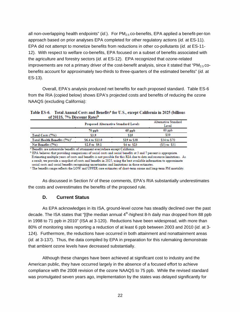
22

all non-overlapping health endpoints” (id.). For PM2.5 co-benefits, EPA applied a benefit-per-ton

approach based on prior analyses EPA completed for other regulatory actions (id. at ES-11).

EPA did not attempt to monetize benefits from reductions in other co-pollutants (id. at ES-11-

12). With respect to welfare co-benefits, EPA focused on a subset of benefits associated with

the agriculture and forestry sectors (id. at ES-12). EPA recognized that ozone-related

improvements are not a primary driver of the cost-benefit analysis, since it stated that “PM2.5 co-

benefits account for approximately two-thirds to three-quarters of the estimated benefits” (id. at

ES-13).

Overall, EPA’s analysis produced net benefits for each proposed standard. Table ES-6

from the RIA (copied below) shows EPA’s projected costs and benefits of reducing the ozone

NAAQS (excluding California):

As discussed in Section IV of these comments, EPA’s RIA substantially underestimates

the costs and overestimates the benefits of the proposed rule.

D. Current Status

As EPA acknowledges in its ISA, ground-level ozone has steadily declined over the past

decade. The ISA states that “[t]he median annual 4th-highest 8-h daily max dropped from 88 ppb

in 1998 to 71 ppb in 2010” (ISA at 3-120). Reductions have been widespread, with more than

80% of monitoring sites reporting a reduction of at least 6 ppb between 2003 and 2010 (id. at 3-

124). Furthermore, the reductions have occurred in both attainment and nonattainment areas

(id. at 3-137). Thus, the data compiled by EPA in preparation for this rulemaking demonstrate

that ambient ozone levels have decreased substantially.

Although these changes have been achieved at significant cost to industry and the

American public, they have occurred largely in the absence of a focused effort to achieve

compliance with the 2008 revision of the ozone NAAQS to 75 ppb. While the revised standard

was promulgated seven years ago, implementation by the states was delayed significantly for

23

the following reason: Following promulgation of the 2008 revised standard, EPA announced, on

September 16, 2009, that it would commence a rulemaking to reconsider the revised 2008

ozone NAAQS.6 As a result, “states were given the impression that if the NAAQS were revised

as a result of the reconsideration, the 3-year deadline [to submit infrastructure SIPs] would be

reset.” 78 Fed. Reg. 34178, 34183 (June 6, 2013). Because many states relied on EPA’s

reconsideration process (see Section II.B.3) and did not submit timely infrastructure SIPs, EPA

was forced by court order to find that 28 States, the District of Columbia, and Puerto Rico failed

to make timely SIP submissions. 78 Fed. Reg. 2882 (Jan. 15, 2013). This finding established a

24-month deadline for EPA to establish federal implementation plans unless the states

submitted approvable infrastructure SIPs before the February 14, 2015 deadline. Thus, as a

result of EPA’s action to reconsider the 2008 ozone NAAQS, development of SIPs was

significantly delayed and many states are still in the process of preparing and implementing

infrastructure SIPs to comply with the revised 2008 standard.

Furthermore, EPA postponed designating areas as attainment, nonattainment, or

unclassifiable for the 2008 NAAQS until more than four years after that standard was

promulgated. 77 Fed. Reg. 30088 (May 21, 2012); 77 Fed. Reg. 34221 (June 11, 2012).

States are only beginning to implement the reduction in the 8-hour ozone NAAQS from 84 ppb

(0.08 ppm) to 75 ppb. Indeed, EPA’s rule explaining its requirements for SIPs for areas that

were designated nonattainment for the current standard was not published in the Federal

Register until March 6, 2015. 80 Fed. Reg. 12263.

Completion of the development and implementation of SIPs to meet the current standard

is continuing to require the expenditure of significant resources by federal, state, and local

regulators and regulated entities. It is expected that such implementation would result in further

reductions in ambient ozone levels. However, EPA is proposing to reduce the standard further

before that task is completed.

E. Impacts of EPA’s Proposed Rule

If finalized, the proposed revisions to the ozone NAAQS will have significant adverse

impacts on members of the Associations, their customers, the communities and states in which

they operate, and the overall U.S. economy. The Associations’ members emit ozone precursors

that are the subject of regulation under the Act, notably NOx and VOCs, and thus will be directly

impacted by any revision to the ozone NAAQS. Promulgation of a revised NAAQS triggers

requirements for state, local, and tribal entities to adopt new NAAQS in their jurisdictions and to

develop NAAQS-specific SIPs to plan for the achievement and maintenance of the revised

6 See EPA, Press Release, EPA Announced it Will Reconsider National Smog Standards (Sept. 16, 2009), available at http://yosemite.epa.gov/opa/admpress.nsf/0/85F90B7711ACB0C88525763300617D0D.

24

NAAQS. See CAA. §§ 110(a)(2) (infrastructure SIPs), 172(c) (general requirements for

nonattainment area SIPs), 182 (specific requirements applicable to SIPs for ozone

nonattainment areas). States and other entities preparing SIPs do not have discretion to target

air quality values that are less stringent than the NAAQS adopted by EPA. As a result, revising

the NAAQS will require states and local communities to commit significant resources to develop

new SIPs and these SIPs will ultimately subject the Associations’ members to costly and more

stringent emissions controls.

Although ambient ozone concentrations continue to decrease, a significant number of air

quality control regions will be unable to attain the proposed NAAQS unless states mandate

additional reductions in emissions of ozone precursors beyond those included in SIPs designed

to attain the current NAAQS of 75 ppb. For example, Figure 1 (presented above) shows areas

that are currently designated nonattainment under the current NAAQS (top panel) and those

that would be projected to be designated as nonattainment areas under a revised standard of

65 ppb based on data for 2011 through 2013 (bottom panel). This figure illustrates the massive

increase in nonattainment areas nationwide that would result from such a reduced standard.

Further, an analysis by the Baton Rouge Area Chamber (copy attached as Attachment A)

shows that, of the nation’s top 20 metropolitan area economies, as ranked by the Brookings

Institution’s assessment of performance through recession and recovery, 15 would be classified

as nonattainment for a 70 ppb standard and 18 of the 20 would be classified as nonattainment

for a 65 ppb standard (compared to 8 for the current standard).

EPA’s own RIA projects that significant emissions reductions beyond the baseline case

will be required to attain the proposed NAAQS. The RIA’s projections (including California)

indicate that a NAAQS of 70 ppb would require NOx emission reductions of approximately

700,000 tons/year and VOC emission reductions of approximately 55,000 tons/year, and that a

NAAQS of 65 ppb would require NOx emission reductions of nearly 2,000,000 tons/year and

VOC emission reductions of approximately 106,000 tons/year (RIA at ES-8 to ES-10). In fact,

the required emissions reductions and associated costs would likely be even greater than EPA’s

projections. This is demonstrated by two recent studies conducted by NERA Economic

Consulting (NERA) – one evaluating the economic impacts of a 65 ppb NAAQS for ozone

(NERA Impacts Report, copy attached as Attachment B) and the other presenting a review of

the RIA’s cost estimates (NERA RIA Review, copy attached as Attachment C). These studies

demonstrate that the RIA significantly underestimates the incremental reduction in emissions of

ozone precursors that will be required if EPA revises the ozone NAAQS and significantly

underestimates the per-ton costs of reducing emissions of ozone precursors. See also Section

IV.A below. As a result, the emission reduction and cost burdens imposed on U.S. businesses

will be even greater than what EPA estimates.

25

EPA acknowledges that existing emission control technologies will not be sufficient to

achieve the proposed NAAQS, and that states, along with the regulated community, will instead

have to rely on what EPA refers to as “unknown controls” to further reduce ambient ozone levels

to achieve attainment with the proposed NAAQS. See RIA at ES-6 & 7-10. The RIA itself

estimates that, for a 65 ppb standard, unknown controls represent over 40 percent of the total

emissions reductions projected by EPA (id. at 4-22 to 2-23, Tables 4-10 & 4-11), but comprise

more than 70 percent of the costs of compliance (see NERA RIA Review at 14-15). In fact, as

shown by the NERA Impacts Report, achievement of such a standard will require greater

reliance on unknown controls than projected in the RIA. For example, that report estimates that

over 60 percent of the emissions reductions to achieve a 65 ppb standard would need to come

from unknown controls. Since these controls are not known, their technological feasibility and

costs are likewise unknown, and the proposed rule could thus lead to the early closure of plants

and the early scrapping of equipment. For example, in California, some air quality management

districts have completely exhausted cost-effective control technologies for reducing ozone

precursors and thus have none left to require.

Moreover, reliance on these unknown emission control technologies could have serious

regulatory repercussions. Under the CAA, the ability to rely on unknown new or improved

technologies is limited to “extreme” nonattainment areas (§ 182(e)(5)). The SIPs for other

nonattainment areas (i.e., moderate, serious, and severe nonattainment areas) must specify

how the NAAQS will be achieved (§§ 182(b), (c), (d)). Thus, if a state is forced to rely on

unknown controls to reduce ambient ozone concentrations to achieve the revised standard in

such areas, EPA may disapprove the SIP and promulgate a federal implementation plan (FIP)

under § 110(c) (or be sued to compel such action), and could impose sanctions under § 179(b),

which can include an increase in the ratio for emissions offsets and/or a cutoff of federal funds

for highway projects. The imposition of such sanctions would have severe adverse impacts for

regulated entities and/or local communities. Alternatively, if the state were to reclassify the area

to extreme nonattainment, that designation would result in the imposition of the more stringent

requirements applicable in such areas (described below), with the associated negative

consequences for regulated businesses.

In short, the need to rely on yet-undefined controls to achieve the proposed revised

standards will further increase the costs and further undermine the technological feasibility of

achieving the proposed standards.

In addition, as discussed in Sections II.C.4 and III.C.1, EPA’s proposed NAAQS may be

at or below background ozone levels for some air quality control regions, meaning that no

amount of technological innovation will allow those regions to reach attainment status. Any

facilities located in such areas will likely face even more severe burdens as states are forced,

however futilely, to reduce emissions as far as possible.

26

Furthermore, the burdens on the Associations’ members and other businesses will not

be limited to those imposed by the states in future SIP revisions. Once a revised standard is

finalized and EPA makes new attainment designations, the Associations’ members and other

members of the regulated community will be subject to more stringent obligations under the

New Source Review (NSR) program. First, for new and modified sources in areas designated

as attainment or unclassifiable – either before or after new attainment designations are made –

granting of a Prevention of Significant Deterioration (PSD) permit will be dependent on a

showing that emissions from the new or modified facility “will not cause, or contribute to, air

pollution in excess of” the revised ozone NAAQS. See CAA § 165(a)(3). A revised NAAQS will

make that showing more difficult. Second, for new and modified sources in regions that are

designated as nonattainment as a result of the revised ozone NAAQS (which, as shown above,

will be greatly expanded over current nonattainment areas), NSR obligations become much

more onerous. Under the Nonattainment New Source Review (NNSR) permitting program, new

and reconstructed facilities must install emission controls that incorporate the Lowest

Achievable Emission Rate (LAER) as opposed to the less stringent Best Available Control

Technology (BACT) requirement applicable to PSD permits. In addition, new and modified

sources subject to NNSR are required to obtain emissions offsets at a greater than 1:1 ratio

from other facilities in the region to ensure that ambient ozone concentrations will not increase

as a result of the project. These more stringent NNSR requirements will impose significant

burdens on the Associations’ members and could stymie economic growth in nonattainment

areas by discouraging the location of new businesses and restricting the growth of existing

businesses in those areas.

Overall, the economic impact of the proposed revisions to the ozone standard will be

unprecedented. The NERA Impacts Report estimates, for example, that over the period from

2017 through 2040, a standard of 65 ppb could cost almost $1.1 trillion (present value), reduce

the U.S. GDP by an average of about $140 billion per year or a total of about $1.7 trillion, result

in a loss of approximately 1.4 million job equivalents, and reduce the average U.S. household

consumption by about $830 per year. All sectors of the economy would be affected by a

reduced standard, both directly through increased emission control costs and/or plant closures

and indirectly through potential impacts on the affected entities’ customers and/or suppliers.

Tables S-9 and S-10 of the NERA Impacts Report present the estimated changes in output for

various sectors of the economy.7

Finally, contrary to EPA’s assertion in the proposed rule, revising the ozone NAAQS will

have a significant effect on energy supply, distribution, and use. EPA claims in the proposed

7 In addition, the solid waste management industry notes that landfills facing cost-prohibitive advanced control equipment requirements will turn to flaring of biogas instead of beneficially using the landfill gas as a source of energy. This will increase overall emissions because equivalent energy generation from fossil fuels will no longer be avoided.

27

rule that revising the ozone NAAQS “is not a significant energy action” under Executive Order

13221 because emissions reduction strategies “will be developed by states on a case-by-case,

basis and the EPA cannot predict whether the control options selected by states will include

regulations on energy suppliers, distributors, or users.” 79 Fed. Reg. at 75386. This assertion

cannot be squared with EPA’s own estimate in the RIA that, to attain a NAAQS of 65 ppb for

example, Electric Generating Units (EGUs) would have to reduce NOx emissions by more than

200,000 tons/year RIA at ES-8, Table ES-2). Given the significant across-the-board emission

reductions that EPA identifies in the RIA, it is inconceivable that the states could all achieve a

revised ozone NAAQS without imposing some additional emission reduction obligations on

EGUs. The NERA Impacts Report points out (at S-12 to S-13) that a 65 ppb standard would

impact U.S. energy sectors, largely because it would lead to the premature retirement of many

coal-fired EGUs, and could cause the average residential cost of electricity to rise by an

average of 1.7% per year through 2040 compared to what it would otherwise be without such a

standard. Thus, it is disingenuous for EPA to assert that it is State SIPs – not the revised

NAAQS – that will affect energy supply, distribution, and use, when EPA leaves the states no

choice but to do so.

III. DEFICIENCIES IN EPA’S PROPOSAL

A. Legal Standard

Section 307(d)(9) of the Act establishes the standard by which EPA’s decisions on

NAAQS will be reviewed in the courts – a standard which is similar to that provided in the

Administrative Procedure Act (5 U.S.C § 706). Under that provision of the Act, an EPA decision

on a NAAQS revision is subject to reversal by the reviewing court if, among other things, it is:

“(A) arbitrary, capricious, an abuse of discretion, or otherwise not in accordance with law”; or

“(C) in excess of statutory jurisdiction, authority, or limitations.” To survive judicial review, an

agency must “articulate a satisfactory explanation for its action including a ‘rational connection

between the facts found and the choice made.’” Motor Vehicle Mfrs. Ass'n of U.S., Inc. v. State

Farm Mut. Auto. Ins. Co., 463 U.S. 29, 43 (1983) (quoting Burlington Truck Lines v. United

States, 371 U.S. 156, 168 (1962)). Further expanding on this standard, the Supreme Court has

held that “an agency rule would be arbitrary and capricious if the agency has relied on factors

which Congress has not intended it to consider, entirely failed to consider an important aspect of

the problem, offered an explanation for its decision that runs counter to the evidence before the

agency, or is so implausible that it could not be ascribed to a difference in view or the product of

agency expertise.” Id.

Applying this standard, courts have vacated agency actions that failed to consider all of

the relevant factors that could influence the agency’s ultimate decision. For example, in Motor

Vehicle Mfrs. Ass’n, the Court considered the National Highway Traffic Safety Administration’s

28

decision to rescind a regulation requiring passive occupant restraint systems, which consisted of

seat belts or airbags. Id. at 37. While the agency sought to justify rescission based solely on

the asserted ineffectiveness of seat belts, the Court vacated the agency’s decision, holding that

“the mandatory passive-restraint rule may not be abandoned without any consideration

whatsoever of an airbags-only requirement.” Id. at 51. Likewise, in a case involving control of

hazardous air pollutants under Section 112, the D.C. Circuit vacated an EPA standard for brick

and ceramic kilns for failure to consider a full range of factors affecting emissions when setting

so-called MACT floors. Sierra Club v. EPA, 479 F.3d 875, 883 (D.C. Cir. 2007). In that case,

EPA had limited its analysis to technology-based emissions controls and failed to evaluate the

role of “non-technology factors [that] affect emission levels.” Id. See also Advocates for

Highway & Auto Safety v. Fed. Motor Carrier Safety Admin., 429 F.3d 1136, 1145 (D.C. Cir.

2005) (setting aside an agency rule on training for commercial vehicle drivers for failure to

consider key study); Pub. Citizen v. Fed. Motor Carrier Safety Admin., 374 F.3d 1209, 1216

(D.C. Cir. 2004) (setting aside an agency rule limiting the driving time and work of commercial

vehicle operators for failure to consider the impact of the rule on the health of drivers, as

required by the statute). As these cases demonstrate, an agency cannot pick and choose from

among relevant factors when deciding whether to revise an existing regulation. It must consider

the full range of factors that are relevant to the decision, either as a result of statutory

obligations or previous regulatory actions. A myopic approach that focuses solely on the factors

that support an agency’s proposed course of action while ignoring countervailing factors will be

vacated.

Nor is it sufficient for an agency to privately consider these factors; it must justify its

decision in the administrative record so that both the courts and the general public can be

assured that the agency considered all of the relevant factors and provided a rational basis for

its ultimate decision. Where the administrative record lacks such a reasoned justification, it

cannot be provided after the fact by the agency or by the courts. Thus, courts vacate or remand

agency decisions when the agency fails to fully explain its decision in the rulemaking record.8

8 See, e.g., Sierra Club v. EPA, 294 F.3d 155, 163 (D.C. Cir. 2002) (“The EPA made no mention of these [challenged emission control] measures or measures like them, . . . . This omission – whether the result of inadvertence or of an unexplained change of course – renders the EPA's decision arbitrary and capricious.”); North Carolina v. EPA, 531 F.3d 896, 917 (D.C. Cir. 2008) (“Nowhere does EPA explain how reducing Title IV allowances will adequately prohibit states from contributing significantly to downwind nonattainment of the PM2.5 NAAQS.”); Arteva Specialties S.a.r.l. v. EPA, 323 F.3d 1088, 1092 (D.C. Cir. 2003) (“EPA may well be correct that the availability of the alternatives it cites adequately answers the petitioners' concern over the cost-effectiveness of the cited provisions. We are unable, however, to discern this from the administrative record because EPA did not take into account these particular alternatives in conducting its cost effectiveness analysis. We therefore have no evidence of their cost or of their effectiveness.”); Mossville Envtl. Action Now v. EPA, 370 F.3d 1232, 1243 (D.C. Cir. 2004) (“While EPA may be able to know that a correlation exists between one known pollutant and some other unknown pollutants, it has not memorialized that knowledge in such a fashion that commenters, interested members of the public, regulated entities, or most importantly, a reviewing court, can assess. We cannot review under any standard the adequacy of the EPA's correlation determination if we do not

29

Thus, an agency cannot simply rely on discretionary freedom or policy judgment to justify its

rules. Even where a court’s ultimate standard of review is deferential, the agency has an

obligation to fully explain how it has elected to exercise that discretion so that the court has a

basis on which to review the agency’s decision.

Moreover, when an agency issues a rule that reverses a prior determination without

providing a proper factual basis that justifies the change, its rule will be found to lack a rational

basis and thus be arbitrary. Otherwise, an agency would be free to change regulatory

obligations based solely on policy reasons. For example, in a case involving attainment

determinations for the 1997 particulate matter NAAQS, the D.C. Circuit vacated EPA’s

nonattainment designation for a county in New York where EPA interpreted the same data in a

different manner in order to justify more stringent regulatory standards. Catawba Cnty., N.C. v.

EPA, 571 F.3d 20 (D.C. Cir. 2009). There, in order to justify a nonattainment decision, EPA

reclassified the county’s commuter numbers from “low” to “significant” even though “there was

no intervening change in the data.” Id. at 52. Similarly, a court vacated a U.S. Forest Service

rulemaking in which the Bush Administration rescinded a “Roadless Rule” that limited

development on certain federal lands. California ex rel. Lockyer v. U.S. Dep't of Agric., 459 F.

Supp. 2d 874, 904 (N.D. Cal. 2006) aff'd, 575 F.3d 999 (9th Cir. 2009). There the court found

that the agency failed to demonstrate any change in facts that would justify a change in the

Roadless Rule. Id. (“Here, the Forest Service reversed course without citing any new evidence

that would lead to a different conclusion or explaining why it had concluded that the protections

of the Roadless Rule were no longer necessary for the reasons it had previously laid out in

detail, and without properly invoking a categorical exclusion.”). As these cases indicate, an

agency cannot simply operate on a blank slate for each successive regulatory action. Instead,

its actions must be informed by prior decisions, and an agency cannot depart from those

decisions for policy reasons when the factual evidence does not support a change.

Finally, of course, an agency rule will be set aside when it contravenes the requirements

of the underlying statute or exceeds the agency’s authority under the statute. See, e.g., Utility

Air Regulatory Group v. EPA, 134 S. Ct. 2427 (2014) (holding that EPA could not lawfully apply

PSD and Title V permit requirements to stationary sources based solely on their potential to

emit greenhouse gases, or alter statutory applicability thresholds for PSD permits in response to

an unlawful interpretation of the Act); Mississippi, 744 F.3d at 1361-62 (holding that EPA’s

secondary ozone standard violated the Act because “EPA failed to determine what level of

protection was ‘requisite to protect the public welfare,’” as required by the Act).

know what correlation the EPA found to exist.”); Bluewater Network v. EPA, 370 F.3d 1, 21 (D.C. Cir. 2004) (“However, we can find nothing in the record indicating that the Agency evaluated or reached any conclusions as to the cost of discontinuing [snowmobile] models to which advanced technology could not be applied by 2012. Absolute certainty and precision on this point are not required, but a reasonable explanation clearly is necessary.”).

30

This section of the Associations’ comments demonstrates that, in several respects,

EPA’s proposed rule revising the NAAQS for ozone, if finalized, would be subject to reversal

under the foregoing standards and case law.

B. EPA’s “Policy Choices” Are Not Insulated from Scrutiny.

In its proposal, EPA states that the selection of a primary standard that is requisite to

protect public health with an adequate margin of safety requires “judgments based on an

interpretation of the scientific evidence and exposure/risk information that neither overstates nor

understates the strengths and limitations of that evidence and information, nor the appropriate

inferences to be drawn therefrom” (79 Fed. Reg. at 75303-04). According to EPA, “[t]he

selection of any particular approach for providing an adequate margin of safety is a policy

choice left specifically to the Administrator’s judgment,” in which EPA “considers such factors

as the nature and severity of the health effects, the size of sensitive population(s) at risk, and

the kind and degree of uncertainties that must be addressed” (id. at 75238 & 75304 n.157;

emphasis added).

EPA’s invocation of “policy choice” and “the Administrator’s judgment” cannot insulate its

decision from scrutiny. While the selection of a primary standard level is ultimately a policy

decision based on the Administrator’s judgments, particularly in the face of the considerable

uncertainties in the scientific information such as exist here, that does not mean that EPA has

discretion to set the standard at any level based on its policy choice. The Agency must still

explain and consistently apply the criteria that will inform that policy decision. As explained in

Section III.A, an agency must provide a reasoned explanation for its decision in the

administrative record. Thus, as the D.C. Circuit has explained, a court cannot review the

adequacy of EPA’s decision if the agency “has not memorialized that knowledge in such a

fashion that commenters, interested members of the public, regulated entities, or most

importantly, a reviewing court, can assess.” Mossville Envtl. Action Now, 370 F.3d at 1243.

Furthermore, the Agency must demonstrate that its policy decision comports with the applicable

legal requirements discussed above – i.e., to set the standard at a level that is sufficient but not

lower than necessary to protect the public health, to set the standard at a level requisite to

protect sensitive subpopulations but not the most sensitive individuals within those

subpopulations, to take account of background concentrations and set the standard at a level

that can be achieved by regulation of sources subject to SIPs. Additionally, EPA needs to give

reasonable consideration to the contextual factors affecting its policy decision, which are within

its authority to consider. See Section II.A above. As shown in the following sections of these

comments, EPA’s proposal to reduce the level of the NAAQS does not meet the foregoing

requirements.

In addition, EPA’s proposal cannot be justified by CASAC’s efforts to constrain the

Administrator’s decision in favor of a more stringent standard by characterizing as science what

31

are in fact policy choices. For example, the basic issue of whether the current standard is

requisite to protect public health depends, in large part, on the interpretation of whether the

responses reported in human clinical studies at lower levels are adverse health effects, the

determination of what levels of risk are acceptable in the general population, and the

determination of how to weigh the uncertainties in the epidemiological studies regarding the

attribution of effects to ozone exposure at levels below the current standard. Those are

ultimately policy judgments for the EPA Administrator. CASAC, however, asserted that “there is

clear scientific support for the need to revise the standard” and “substantial scientific certainty of

a variety of adverse effects” at 70 ppb (Frey, 2014, pp. ii, 8) when it is clear that its conclusions

are actually based on its interpretation of the evidence and its views on the above-mentioned

policy issues. Additionally, as both EPA and even CASAC appear to recognize, the

determination of an adequate margin of safety is a policy judgment, not a scientific judgment

(see 79 Fed. Reg. at 75303; Frey, 2014, p. ii), and thus CASAC’s views on the adequacy of the

margin of safety should have little weight. All of these issues are policy issues for EPA to

decide; and as shown in the prior paragraph, EPA’s decision on those issues must comply with

applicable requirements and be adequately justified and is subject to scrutiny as to whether it

has done so.9

C. EPA Has Failed To Give Adequate or Proper Consideration to Background Air Quality.

As explained in Section III.A above, a central tenet of reasoned agency decision-making

is that an agency must consider all of the factors required by Congress. Motor Vehicle Mfrs.

Ass’n, 463 U.S. at 43. Thus, it is arbitrary and capricious for EPA to consider only a subset of

relevant factors, while ignoring or providing an inadequate explanation of others. See, e.g.,

Sierra Club v. EPA, 479 F.3d at 883 (vacating EPA standard that evaluated only technology-

based emission controls while ignoring emissions reductions from non-technology factors that

affect emissions levels). Here, in proposing to reduce the level of the NAAQS for ozone, EPA

has failed to take into account the extent to which the lowered standard would be infeasible to

achieve due to background ozone concentrations, which is a key consideration under the Act.

Moreover, in this case, setting a standard at a level that may be impossible to achieve due to

background concentration conflicts with the statutory requirement, discussed in Section II.A, that

NAAQS be set at levels that can be achieved through state regulation under SIPs, and such a

standard would thus be unlawful. Further, as explained below, EPA cannot simply ignore

background ozone concentration at the standard-setting stage by claiming that it is building in

flexibility at the implementation and enforcement stage. Putting aside the fact that those

responses are wholly inadequate, EPA cannot simply pass the buck on the statutory

requirement when setting the NAAQS in the first instance.

9 Likewise, CASAC’s review of drafts of the EPA staff documents (i.e., the ISA, the HREA, the WREA, and the PA) cannot isolate the conclusions reached in those documents by EPA from further scrutiny.

32

1. EPA Has Unlawfully Failed To Take into Account That Background Ozone Levels Can Prevent Attainment of the Proposed NAAQS.

Ozone’s presence in this nation’s ambient air is attributable to a number of causes.

Anthropogenic emissions of ozone precursors – including VOCs, NOx, CH4, and CO – in the

United States contribute to the formation of ozone (see 79 Fed. Reg. at 75241). Ozone in

ambient air may also result from natural sources such as lightning, wildfires, and vegetative

emissions or occasionally, at higher elevations, from atmospheric intrusions from the

stratospheric ozone layer (id. at 75241). Furthermore, ozone in the U.S. can result from

transport of ozone and ozone precursors from other countries. In the context of setting NAAQS

for ozone, the term “background” must refer to ozone that results from events other than human

activities in the U.S. that lead to the emission of ozone precursors (see id. at 75242). No other

approach makes sense, since those are the only activities that are subject to regulation under

SIPs.10

Background ozone levels are variable (see PA at 2-17), but they can be substantial.

EPA reports seasonal mean background concentrations of as much as 50 ppb (PA at 2-18).

Peak 8-hour average background levels – those matching the averaging time for the present

and proposed ozone NAAQS – are necessarily higher than the overall seasonal average. In

fact, as EPA recognizes, background levels can cause exceedances of even the present ozone

NAAQS:

“[O]bservational and modeling analyses have concluded that [ozone]

concentrations in some locations in the U.S. can be substantially influenced by

sources that may not be suited to domestic controls measures. In particular,

certain high-elevation sites in the western U.S. are impacted by a combination of

non-local sources like international transport, stratospheric [ozone] and [ozone]

originating from wildfire emissions. . . . [T]here can be episodic events with

substantial background contributions where [ozone] concentrations approach or

even exceed the level of the current NAAQS (i.e., 75 ppb).” 79 Fed Reg. at

75242.

10 As mentioned above, in its most recent prior review of the ozone NAAQS, EPA focused on PRB, which it defined as “the [ozone] concentrations that would be observed in the U.S. in the absence of anthropogenic emissions of precursors (e.g., VOC, NOx, and CO) in the U.S., Canada, and Mexico” (73 Fed. Reg. at 16443 n.13), when discussing ozone background. The alternative focus here on what EPA sometimes calls “U.S. Background” (i.e., ozone levels that are not attributable to anthropogenic activities in the U.S.) is appropriate. The Act relies primarily on states to implement NAAQS, CAA §§ 107(a), 110(a)(1), 172(b). States have no authority over emissions that originate in Canada or Mexico. Moreover, the rigid schedules that the Act imposes for states to bring areas into compliance with NAAQS or face sanctions (CAA § 181) are inconsistent with the time required for the negotiation, formalization, and implementation of agreements with Canada and Mexico to implement emission controls to contribute to timely attainment in states in the U.S.

33

A recent study conducted in Clark County, Nevada confirms this. It reports:

“The mean surface [maximum daily 8-hour average] ozone at Jean, NV in rural

Clark County was 67 ppbv during May and June of 2013, which is only 8 ppbv

less than the current 2008 NAAQS and greater than some values that are

currently being considered. . . . The number of days in Clark County during the

43-day [Las Vegas Ozone Study (LVOS)] field campaign would have increased

from 3 to 14 if the NAAQS had been 70 ppbv instead of 75 ppbv, and from 3 to

25 if the NAAQS had been 65 ppbv. In other words, exceedances of the NAAQS

generated by high background concentrations and stratospheric intrusions would

have occurred on 60% of the days during LVOS, making these events the rule

rather than the exception.” (Langford et al., 2014)

Similarly, Zhang et al. (2011) reported “some occurrences” of background ozone levels above

60 ppb, particularly in the West, as shown in Figure 7 of that paper, and noted that if the

NAAQS were reduced to the 60-70 ppb range, “areas of the intermountain West will have little

or no ability to reach compliance through North American regulatory controls.”

Nor are high background concentrations limited to the Intermountain West or to high

elevations. EPA has explained that high background concentrations are also found in northern

New York and “other areas bordering Canada and Mexico” (ISA at 2-6), and figures in its PA

(Figures 2-12 and 2-13) show significant contributions of background (over 50%) to seasonal

means at sites throughout the country (PA at 2-22). The Agency has also recognized that “the

influence of background sources on high surface [ozone] concentrations is not always confined

to high elevation sites,” particularly in areas impacted by ozone formed due to emissions from

Asia (ISA at 3-39). Moreover, the contribution of emissions from Asia to background is likely to

increase, given that Asia, in particular eastern Asia, has the world’s highest growth rate for

emissions of ozone precursors (Cooper et al., 2010). In addition, Lefohn et al. (2012, 2014)

have shown high background concentration sites at various locations throughout the country –

not limited to the Intermountain West or high-elevation sites.

In recent comments submitted on the proposed rule, EPRI (2015) shows, using the

GEOS-Chem model, that U.S. background ozone concentrations have been steadily increasing

in the western and southwestern U.S. (including in cities such as Denver, Los Angeles, and

Phoenix) and are predicted to continue to increase, at least through 2020, due to increased

emissions from Asia and Mexico. These concentrations are predicted to reach 4th highest daily

maximum 8-hour levels close to 65 ppb in some locations, thus making it difficult, if not

impossible, to attain the proposed reduced standards through controls on U.S. sources.11

11 Moreover, since NOx is not only an ozone precursor but also destructive of ozone, a reduction in anthropogenic NOx emissions in an effort to meet a lowered standard will also have the effect of

34

Given the proximity of background ozone levels to the present NAAQS and the more

stringent alternatives that EPA has proposed, the role that background pollutant levels play in

determining the appropriate level for a NAAQS is a key question in this rulemaking. EPA

recognizes that the Act does not require the Agency to set NAAQS at background levels (79

Fed. Reg. at 75238), and acknowledges that it “may consider proximity to background levels as

a factor in the decision whether and how to revise the NAAQS when considering levels within

the range of reasonable values (id. at 75242). Nevertheless, the Agency asserts that it must

“set the NAAQS at levels requisite to protect public health and welfare without regard to the

source of the pollutant” (id. at 75242; emphasis added). Thus, when explaining the decision

to propose to reduce the level of the primary NAAQS from 75 ppb to within the range of 70 ppb

to 65 ppb, EPA does not acknowledge that background ozone levels would, at least in some

locations, approach or potentially exceed the level of a NAAQS within this range.12 Further, by

evaluating exposures and risks from all sources, including background, EPA’s HREA fails to

characterize the exposures and risk that could be addressed by a change in the NAAQS.

Indeed, as concentrations get closer and closer to background, the percentage of the overall

risk that can be addressed by NAAQS becomes smaller and smaller.

In this regard, EPA has misinterpreted both the Act and the relevant case law. As

mentioned in Section II.A, the Act places the burden on “each state” to develop a plan

specifying how the NAAQS “will be attained and maintained” (§ 107(a); emphasis added).

Background ozone, pollution that is attributable either to natural phenomena or to emissions

from outside of the U.S., is plainly beyond a state’s (or EPA’s) control. Congress did not intend

to require states to do the impossible. Indeed, in its report on the 1977 Amendments to the Act,

the House of Representatives specifically explained that it did not intend NAAQS to be set at

background levels. See H.R. Rep. No. 294, 95th Cong., 1st Sess. 127 (1977) (“Some have

suggested that since the standards are to protect against all known or anticipated effects and

since no safe thresholds can be established, the ambient standards should [b]e set at zero or

background levels. Obviously, this no-risk philosophy ignores all economic and social

consequences and is impractical.”).

decreasing the ability of NOx to reduce background concentrations, such that background ozone will become a larger relative contributor to total ozone concentrations as the absolute abundance of background ozone increases. 12 EPA only mentions background in passing in its justification for not considering further standards more stringent than 65 ppb (see 79 Fed. Reg. at 75310). It apparently believes that the Agency has policies in place adequate to provide regulatory relief for situations in which background ozone would lead to NAAQS exceedances (id. at 75242, 75382-85). The availability of such regulatory relief, even if it were useful, would not excuse EPA’s failure to take background ozone levels properly into account in revising the NAAQS, as discussed herein. See Prill v. NLRB, 755 F.2d 941, 948 (D.C. Cir. 1985). Moreover, as discussed in Section III.C.2, the cited policies do not provide significant relief for situations in which background ozone leads to NAAQS exceedances.

35

Against this clear Congressional direction that NAAQS should not be set at background

levels, EPA cites API v. Costle, 665 F.2d 1176, 1184-86 (D.C. Cir. 1981). According to EPA,

this 30-year-old case, which was decided when ozone levels were dramatically higher than they

are today (see Air Quality Trends, http://www.epa.gov/airtrends/aqtrends.html, noting a 33%

decline in 8-hour ozone levels between 1980 and 2013), stands for the propositions that (1)

attainability is not a relevant consideration in promulgation of NAAQS, and (2) “EPA need not

tailor the NAAQS to fit each region or locale” (79 Fed. Reg. at 75239).

However, in addressing attainability, the API court focused on cost and technological

feasibility, not on other factors that render attainment impossible. The court merely quoted its

more lengthy discussion in Lead Industries Ass’n that "’the Administrator may not consider

economic and technological feasibility in setting air quality standards’” (665 F.2d at 1185,

quoting 647 F.2d at 1149). To the extent that it addressed unattainability resulting from other

factors, the court was addressing an argument by the city of Houston that natural factors make

attainment impossible in that area, and the court simply decided that Houston’s particular

circumstances were not a basis for vacating a national standard. See API, 665 F.2d at 1186

(“[T]he agency need not tailor national regulations to fit each region or locale.”). We are not

claiming here that EPA is required to tailor the NAAQS to fit particular areas, but rather that EPA

is required, in issuing nationally applicable NAAQS, to consider the impact of background levels

on the attainability of those national standards. The court in API did not address the issue of

whether a NAAQS that was unattainable not just in a single locale such as Houston, but

throughout much of the nation due to factors beyond the control of the states or even regulated

industries would be consistent with the Act.

In fact, in subsequent decisions, the court suggested that setting a standard that could

not be achieved due to such uncontrollable background levels may be inappropriate. In the first

American Trucking Ass’ns opinion, the court addressed EPA’s support of the 1997 ozone

NAAQS on the ground that a lower standard would be “’closer to peak background levels that

infrequently occur in some areas due to nonanthropogenic sources of O3 precursors.’”

American Trucking Ass’ns v. EPA, 175 F.3d 1027, 1036 (D.C. Cir. 1999), reversed in part and

affirmed in part on other grounds in Whitman, 531 U.S. 457 (2001). The court stated: “EPA’s

language, coupled with the data on background ozone levels, may add up to a backhanded way

of saying that, given the national character of the NAAQS, it is inappropriate to set a standard

below a level that can be achieved throughout the country without action affirmatively

extracting chemicals from nature. That may well be a sound reading of the statute, but EPA

has not explicitly adopted it.” 175 F.3d at 1036 (first emphasis by court; second emphasis

added). Further, as mentioned in Section II.B.1, following remand from the Supreme Court, the

D.C. Circuit again relied, in part, on EPA’s determination that a standard of 70 ppb was too

close to background, and stated that the “relative proximity to peak background ozone

36

concentrations” was a factor that “EPA could consider” when choosing among alternative levels.

American Trucking Ass’ns, 283 F.3d at 379.

The present situation directly raises the issue of potential widespread unattainability of

the proposed revised NAAQS in many parts of the country due to background levels that are not

subject to control under SIPs. Revising the NAAQS without appropriately taking that issue into

account would ignore a key factor for setting the NAAQS at the requisite level, rendering the

NAAQS revision arbitrary and capricious. See Motor Vehicle Mfrs. Ass’n, 463 U.S. at 43, and

other cases cited in Section III.A. In fact, setting an NAAQS that could not be attained in many

parts of the country due to background levels would be inconsistent with the Act’s text and

legislative history and thus would be illegal.13

2. EPA Is Not Planning Effective Regulatory Relief from Nonattainment Due to Background Ozone.

Instead of taking unattainability due to background levels into account in determining the

appropriate level of the ozone NAAQS, EPA identifies three programs that it claims it will use to

provide regulatory relief for situations in which ozone levels “approach or exceed the

concentration levels being proposed in this notice (i.e., 60-70 ppb) in large part due to

background sources.” 79 Fed. Reg. at 75382. Specifically, EPA discusses use of (a)

exceptional event exclusions, (b) treatment as rural transport areas, and (c) international

transport provisions. 79 Fed. Reg. at 75383-85. The availability of such regulatory

mechanisms, even if they were useful, would not excuse EPA’s failure to take background

ozone levels properly into account in revising the NAAQS. Moreover, these regulatory

mechanisms would not, in fact, provide any significant relief from NAAQS exceedances due to

background ozone levels. While each of these provisions could in theory provide limited relief

from such exceedances, each has been a part of the Act for a decade or more without being

used effectively by EPA. As discussed below, they provide little hope of relief if EPA adopts a

more stringent NAAQS that is even more likely to be exceeded as a result of background ozone.

This demonstrates further that EPA’s identification of these regulatory mechanisms is no

substitute for taking background into account in setting the level of the standard.

a. EPA’s Exceptional Events Program Has Not Been Successful.

Section 319(b), which was added to the Act in 2005, required EPA to develop

regulations to govern the review and handling of monitored air quality data influenced by

exceptional events, including specification of “criteria and procedures” for states to use when

13 CASAC was not informed that setting a NAAQS at or below background levels would be illegal, and indeed questioned the role of background levels in setting NAAQS. See letter from the CASAC Chair to EPA dated June 26, 2014 (Frey, 2014) (“The Second Draft PA was silent as to how the EPA intends to navigate between these two legal guidelines when considering background ozone in a policy and standard-setting context. This question became an important issue in the CASAC deliberations . . . . ”).

37

petitioning for the exclusion of monitoring data “that is directly due to exceptional events” from

consideration when judging NAAQS exceedances or violations (§ 319(b)(2)(B), (b)(3)(B)(iv)).

EPA’s Exceptional Events Rule (EER) was published in 2007. 72 Fed. Reg. 13560 (March 22,

2007)). Although EPA now suggests that the EER provides “regulatory relief” from NAAQS

exceedances due to background (79 Fed. Reg. at 75382-83), the Agency has previously

specifically disavowed that role for the EER. EPA’s Draft Guidance on the Implementation of

the EER stated: “Exceedances due to natural emissions that occur every day and contribute to

policy relevant background, such as biogenic emissions, do not meet the definition of an

exceptional event and are thus not eligible for exclusion under the EER. Routine anthropogenic

emissions outside of the U.S. contribute to policy relevant background, but are not exceptional

events.” 77 Fed. Reg. 39959 (July 6, 2012). Similarly, in a memorandum dated May 10, 2013

from Stephen D. Page, Director of EPA’s Office of Air Quality Planning and Standards, to

Regional Air Directors, EPA stated that “the demonstration to justify data exclusion shall provide

evidence that the event is associated with a measured concentration in excess of normal

historical fluctuations, including background” (Page, 2013, at 3; emphasis added).

Even if EPA intended the EER to be used to address NAAQS exceedances attributable

to background, however, it has not been an effective tool for doing so. Although the EER was

published almost eight years ago, EPA’s website indicates that the Agency has granted only

three exceptional event determinations under it with regard to ozone, one concerning

stratospheric ozone intrusion and two related to fires.14

States have expressed frustration with EPA’s implementation of the Act’s exceptional

events provision. Recently, for example, Utah’s senators and representatives wrote to the EPA

Administrator:

EPA’s reliance . . . on the Exceptional Events Rule (EER) to deal with high ozone

background “episodes” effectively condemns the intermountain West to “guilty

until proven innocent” and incurs a high resource burden to meet the “but for”

demonstration. The EER has not been effective to date in excluding background

concentrations from determination of NAAQS attainment. The application by

Utah for EER exclusions have routinely been denied by EPA regional officials

following years of work by state and industry staff. (Hatch et al., 2014.)

They quoted testimony by the Executive Director of Utah’s Department of Environmental

Quality, Amanda Smith, in 2013:

14 EPA, Exceptional Events Submissions Table, available at http://www.epa.gov/ttn/analysis/exeventstable.htm (last visited March 5, 2015).

38

Since 2008 Utah has submitted 12 exceptional event demonstrations for

particulate matter, requiring about 4,000 hours of technical work, that have not

been approved by [EPA] Region 8. There were many other events, including

ozone levels affected by western wildfires that we did not even attempt to

demonstrate as exceptional events because the technical criteria were too

difficult to meet. If the exceptional event process doesn’t work for particulate

matter – it certainly won’t work for the complicated science behind rural

background ozone. (Smith, 2013.)

Although Ms. Smith’s testimony focused on the difficult technical criteria for obtaining an

exceptional event determination, EPA’s interpretation of the Act is also unreasonably

constrained. Thus, EPA interprets the EER to exclude ozone attributable to “natural emissions

from vegetation, microbes, animals, and lightning” from exceptional event treatment. 79 Fed.

Reg. at 75383 n.274. The Act, however, defines exceptional events as those affecting air

quality that are “not reasonably controllable or preventable” and are due to “an event caused by

human activity that is unlikely to recur at a particular location or a natural event” (§

319(b)(1)(A); emphasis added). Elevated ozone levels due to natural emissions would certainly

appear to quality for treatment as exceptional events under this statutory definition. However,

EPA’s unduly narrow interpretation of the Act – in conjunction with the unreasonable technical

demonstration burdens imposed by its EER – renders the statutory exceptional events provision

virtually useless.

b. The CAA Provision Concerning Rural Transport Areas Has Not Historically Provided Effective Relief for Ozone Nonattainment Areas.

Section 182(h) allows EPA to determine, at its discretion, that an ozone nonattainment

area is subject only to the requirements applicable to a “marginal” area (rather than those

applicable to an area with a higher classification) if (1) the area in question is not in or adjacent

to a Metropolitan Statistical Area (MSA) or Consolidated Metropolitan Statistical Area (CBSA),

and (2) does not contain sources of VOC or NOx emissions that “make a significant contribution

to” ozone concentration in that or another area (§182(h)). EPA notes in the proposed rule that,

“[h]istorically, the EPA has recognized few nonattainment areas under this statutory provision.”

79 Fed. Reg. at 75384. This is an understatement. Although EPA classified three areas as

“rural transport” areas for the 1-hour ozone NAAQS,15 no area has ever been designated as a

15 EPA mentions only Essex County, New York, and Smyth County, Virginia in the proposed rule (79 Fed. Reg. at 75384 n.284), but the Agency’s Technical Support Document for designations for the 1-hour NAAQS also identifies Door County, Wisconsin as a rural transport area for ozone. Technical Support Document for Ozone and Carbon Monoxide Designations and Classifications Under Section 107(d) of the Clean air Act Amendments or 1990, at 52 (Oct. 1991), available at http://www.epa.gov/airquality/ozonepollution/designations/1997standards/tech.htm (follow “Chapter 6: additional Supporting Documents” hyperlink, then go to page 728).

39

rural transport area with regard to an 8-hour NAAQS. Further, with the proposed decrease in

the primary and secondary standards and the corresponding increase in the number and size of

nonattainment areas adjacent to MSAs and CBSAs, the prospects of being able to use the

Section 182(h) authority in a meaningful way grow even dimmer.

EPA initially planned an “overwhelming transport” classification for nonattainment areas

for the 1997 8-hour NAAQS that would be implemented under Subpart 1 of Part D of Title I of

the Act. See 68 Fed. Reg. 23951, 23964 (Apr. 30, 2004). Even before the Agency’s plan to use

Subpart 1 to implement the NAAQS was rejected by the court,16 however, EPA backed away

from such a classification, since the Agency had agreed to reconsider it. 71 Fed. Reg. 15098

(Mar. 27, 2006).17 For nonattainment areas that EPA planned to address under Subpart 2 of

Part D of Title I of the Act, the Agency indicated that it “did not believe that there are any 8-hour

nonattainment areas covered under subpart 2 that are ‘rural’ and therefore eligible for

consideration of coverage under section 182(h).” 70 Fed. Reg. 71612, 71623 (Nov. 29, 2005).

More recently, in its March 2015 SIP rule for nonattainment areas for the 2008 ozone NAAQS,

EPA noted the existence of Section 182(h), but explained that it had not identified any rural

transport areas “during the designations process” (80 Fed. Reg. at 12292 & n.64).

Furthermore, while pointing to the rural transport provision in the proposed rule as a

potential source for appropriate regulatory relief, EPA at the same time limits its usefulness.

First, the Agency explains that it will not consider any rural area with a monitor “heavily

influenced by short-range upwind contributions from a nearby urbanized area” a candidate for

relief as a rural transport area (79 Fed. Reg. at 75384 n.277). In doing so, EPA is

administratively limiting the scope of the relief that Congress provided for rural transport areas.

Second, EPA cites with approval draft guidance requiring that a demonstration to support a rural

transport classification must include “assembling emissions, air quality, meteorological and/or

photochemical grid modeling data” and must describe “analyses performed, data bases used,

key assumptions and outcomes of each analysis, and why a State believes that the evidence,

viewed as a whole, supports a conclusion that the area is overwhelmingly affected by transport

and does not significantly contribute to downwind problems.”18 This guidance would impose a

substantial analytical burden on a state in preparing its designations that must be submitted to

16 S. Coast Air Quality Mgmt. Dist. v. EPA, 472 F.3d 882, 892 (D.C. Cir. 2006), modified 489 F.3d 1245 (D.C. Cir. 2007). 17 At that time, EPA sought comment on its draft guidance on “Criteria For Assessing Whether an Ozone Nonattainment Area is Affected by Overwhelming Transport” (71 Fed. Reg. at 15100),calling into question the continuing viability of that draft. Nevertheless, EPA cites that uncertain draft guidance in the proposed rule (79 Fed. Reg. at 79384 & n.279), as discussed below. 18 79 Fed. Reg. at 79384 & n.279 (citing EPA, Criteria for Assessing Whether an Ozone Nonattainment Area is Affected by Overwhelming Transport 3 (Draft June 29, 2005), available at http://www.epa.gov/ttn/scram001/guidance/guide_guidance_07-13-05.pdf).

40

EPA within a year after the Agency’s promulgation of a revised NAAQS and would likely

discourage states from seeking the rural transport classification.

In short, no ozone nonattainment area has been classified as a rural transport area for

almost 14 years, despite increasingly stringent standards over that period. Further, while citing

that classification as a potential source of regulatory relief for areas facing nonattainment

designations as a result of background ozone level, EPA now seeks to limit the applicability of

the rural transport classification further and to impose substantial burdens on states that might

seek to use it. As a result, it is disingenuous to conclude that this provision will provide effective

relief should EPA now adopt an even more stringent NAAQS.

c. The Act Provides Only Limited Relief for Areas that Would Not Meet a More Stringent Ozone NAAQS Due to International Transport of Ozone and Ozone Precursors.

Section 179B, titled International Border Areas, requires EPA to approve a SIP submittal

for a nonattainment area if (1) the submittal meets all the applicable requirements except “a

requirement that such plan or revision demonstrate attainment and maintenance of the relevant

[NAAQS]” by the applicable attainment date, and (2) the state demonstrates that the SIP “would

be adequate to attain and maintain the relevant [NAAQS]” by that date “but for emissions

emanating from outside of the United States” (§ 179B(a)). For ozone specifically, if those

conditions are met, the Act provides exemptions from Section 181(a)(2) (establishing a severe-

17 classification),19 Section 181(a)(5) (providing for two possible 1-year extension of the

attainment date), and Section 185 (concerning failure of severe and extreme nonattainment

areas to achieve timely attainment (§ 179B(b)).

As recognized in the proposed rule, this provision cannot be used to avoid a

nonattainment designation or as the basis for a lower classification for a nonattainment area, but

only to avoid “adverse consequences” for failing to attain the NAAQS by the applicable deadline

(79 Fed. Reg. at 75384). In other words, states to which this provision is applicable get only

limited regulatory relief. They must still adopt a SIP that addresses the control requirements

associated with the initial classification for the area (e.g., reasonable further progress plans and

nonattainment new source review provisions that utilize a more stringent definition of a major

source) (see § 181(a)-(d)).

EPA does not define what information will be required for a state to establish that an

area qualifies for relief because of the impact of background ozone attributable to international

19 EPA has suggested that this statutory reference is intended to be to Section 181(b)(2) of the Act, which concerns reclassification upon failure to attain, instead of to Section 181(a)(2). 68 Fed. Reg. 32802, 32829 n.38 (June 2, 2003). This suggestion is sensible, but the Agency has provided no support for it.

41

transport. EPA has repeatedly indicated that it will review requests for relief under Section 179B

on a case-by-case basis. See 78 Fed. Reg. at 34205; 70 Fed. Reg. at 71624. Although the

proposed rule refers to a 1991 guidance document on “Criteria for Assessing the Role of

Transported Ozone/Precursors in Ozone Nonattainment Areas” (1991 Guidance) for use in

Section 179B demonstrations (79 Fed. Reg. at 75384 & n.280), EPA previously “retracted” that

guidance.20 Thus, states face an undefined – but potentially heavy – burden in qualifying for the

limited relief provided by this provision of the Act. It is therefore not surprising that the proposed

rule identifies only one instance in which EPA relied on Section 179B to approve an ozone SIP

and none within the past decade.21

In short, none of the options that EPA has identified as providing future regulatory relief

when background leads to exceedances of a revised ozone NAAQS has consistently provided

such relief in the past. Indeed, EPA has previously and unnecessarily limited the applicability of

these provisions and continues to do so in the proposed rule. The theoretical availability of

these tools cannot excuse EPA’s proposal to reduce the level of the ozone NAAQS illegally to

one that is below background levels in many areas.

D. EPA Has Failed to Provide a Reasoned Explanation for Its Change in Interpretation of the Relevant Public Health and Welfare Science.

As discussed in Section II.B.2, in adopting the current primary standard of 75 ppb in

2008, EPA relied on three main bases: (1) The “strong body of clinical evidence” of lung

function decrements, respiratory symptoms, and other airway responses in healthy subjects at

exposure levels of 80 ppb and above, as well as “some indication of lung function decrements

and respiratory symptoms at lower levels”; (2) the clinical evidence indicating that asthmatics

are “likely to experience larger and more serious effects than healthy people”; and (3) the

epidemiological evidence indicating associations for “a wide range of serious health effects “ at

and below 80 ppb (73 Fed. Reg. at 16476). Based on these principal considerations, EPA

made the judgment that a standard of 75 ppb was “requisite to protect public health with an

adequate margin of safety, including the health of sensitive subpopulations, from serious health

20 EPA cited the 1991 Guidance in its 2003 Proposed Rule To Implement the 8-Hour Ozone National Ambient Air Quality Standard in conjunction with its proposal to create an “overwhelming interstate transport classification.” 68 Fed. Reg. 32802, 32814 n.15 (June 2, 2003). When it promulgated the Phase I implementation rule, however, in the context of discussing its decision to provide an “overwhelming transport” classification, EPA ‘retracted” the 1991 “guidance document “ referenced in the June 2, 2003 Proposed Rule. 69 Fed. Reg. 23951 23965 (April 30, 2004). 21 79 Fed. Reg. at 75835. In that instance, which concerned the 1-hour ozone NAAQS, EPA approved the demonstration only after the area had already attained the NAAQS, as shown through air quality monitoring, 69 Fed. Reg. 32450, 32451-52 (June 10, 2004), and thus the role of Section 179B is unclear. Further, EPA indicated at that time that “all section 179B approvals should be on a contingent basis” and are “valid only as long as the area’s modeling data continue to show . . . attainment, but for emissions from outside the United States” (id. at 32452).

42

effects,” and that a lower standard was not needed or warranted (id. at 16483). The court in

Mississippi upheld that judgment.

As discussed above in Section II.B.5, while some new studies have become available

since 2008, they do not alter in any basic way the information on which EPA relied in 2008. As

EPA states in its 2014 proposal, the strongest body of evidence on the occurrence of effects in

healthy subjects in clinical studies still comes from studies of ozone exposures at and above 80

ppb (79 Fed. Reg. at 75304). While two new controlled human exposure studies were

published (Schelegle et al., 2009; Kim et al., 2011), they do not change the fact that, as EPA

stated in 2008, the evidence provides “some indication” of lung function decrements and

respiratory symptoms at lower levels, given that the effects reported in those two studies were

admittedly small – namely, a mean FEV1 decrease of approximately 5% and a modest increase

in subjective symptoms at 72 ppb in Schelegle et al. (2009) and a mean FEV1 decrease of less

than 2% and no increase in subjective symptoms at 60 ppb in Kim et al. (2011). As such, these

studies do not provide any new basic information regarding the types or magnitude of subjects’

responses at these levels. Further, EPA continues to claim that asthmatics are likely to

experience larger and more serious effects than healthy people (79 Fed. Reg. at 75288), but it

recognizes that there are no new clinical studies on this topic (id. at 75272). Additionally, while

there are some new epidemiological studies, EPA continues to acknowledge that there remain

uncertainties regarding the extent to which the effects reported in those studies can be

attributed to ozone exposures below the current standard level, and it thus puts less reliance on

them (see Section II.C.1 above). Recent comments by Gradient (2015) show further that the

new health effects evidence cited in EPA’s proposal does not differ substantially from the

evidence cited in the previous ozone NAAQS review.

Similarly, as discussed in Section II.C.2, above, EPA acknowledges in the proposed rule

that “[t]he current body of [ozone] welfare effects evidence confirms the conclusions reached

in the last review on the nature of [ozone]-induced welfare effects” (79 Fed. Reg. at 75314;

emphasis added). No significant scientific advances have occurred since the prior review that

reduce key uncertainties that were identified during the last review (see id. at 75314,75316,

75317, 75319). See also Gradient (2015).

EPA must provide a reasoned explanation for a change in judgment. EPA may not

reverse prior policy decisions without providing a reasoned explanation for the change. Dillmon

v. NTSB, 588 F.3d 1085, 1089-90 (D.C. Cir. 2009) (citing FCC v. Fox Television Stations, Inc.,

129 S. Ct. 1800, 1811 (2009)) (“Reasoned decision making … necessarily requires the agency

to acknowledge and provide an adequate explanation for its departure from established

precedent.”); see also Motor Vehicle Mfrs. Ass’n, 463 U.S. at 42; AT&T Corp. v. FCC, 236 F.3d

729, 736-37 (D.C. Cir. 2001) (reasoned decision-making standard requires explanation for

departure from prior decision); Troy Corp. v. Browner, 120 F.3d 277, 286 (D.C. Cir. 1997) (citing

43

Nat’l Ass’n for Better Broadcasting v. FCC, 849 F.2d 665, 669 (D.C. Cir. 1988)) (“an agency is

obligated ‘not to depart without reasoned explanation from its prior conclusions.’”). Indeed, as

discussed in Section III.A and shown by the cases cited there, when an agency issues a rule

that changes a prior determination without providing a proper factual basis justifying the change,

its rule will be held to be arbitrary. See, e.g., Catawba Cnty., 571 F.3d at 52; California ex rel.

Lockyer, 459 F. Supp. 2d at 904.

In the case of ozone, as discussed above, the main change since EPA’s last review in

2008 is EPA’s interpretation of the evidence – i.e., its definition of the level of protection that is

“requisite” to protect public health and welfare – not the basic evidence itself. In other words,

given the absence of any fundamental change in the scientific understanding of ozone effects,

EPA appears to have determined simply that levels of risk that were judged acceptable in the

prior standard-setting exercise are no longer acceptable.22

While EPA’s proposal contains lengthy discussions of the scientific evidence, including

the new studies, it does not present a reasoned explanation or justification for this apparent

change in the policy judgment regarding the level of risk that is acceptable – i.e., for why levels

of risk judged acceptable in 2008 are no longer consistent with a proper legal interpretation of

the risk level consistent with “requisite” protection of public health and welfare. Without such a

reasoned explanation, EPA’s adoption of a revised standard would be arbitrary and

capricious.23

E. EPA’s Revision of the Standard Prior to Completion of Implementation of the Current Standard Would be Arbitrary.

As discussed in Section II.D, the current ozone NAAQS of 75 ppb adopted in 2008 has

not been fully implemented. Federal, state, and local regulators are still working on revising

SIPs to implement that standard. As a result, there has not been time to assess the impacts

and asserted health benefits from implementation of that standard.

At the same time, as shown in Section II.B.5 and III.D, commenters have pointed out

that the new scientific information that has become available since the adoption of the current

standard is relatively limited and does not fundamentally alter the understanding of ozone

22 A similar consideration applies with respect to the consideration of background levels. As discussed in Section II.B.1, in setting the 1997 NAAQS, EPA relied in part on the fact that a standard of 70 ppb would be too close to background. However, EPA has apparently now concluded that, despite such proximity to background (which remains true), setting at standard at 70 ppb or below is appropriate. EPA has not provided an explanation for that change in interpretation. 23 Although a similar challenge to the 2008 NAAQS was rejected by the D.C. Circuit in Mississippi (744 F.3d at 1343-44), the Associations submit that EPA nonetheless has an obligation to present a reasoned explanation for such a change in judgment.

44

effects on public health and welfare. Further, as discussed in Sections II.B.5 and II.C, a number

of commenters have pointed out, and EPA itself recognizes in its proposal, that there remain

considerable uncertainties regarding the occurrence of adverse health and welfare effects at

ozone levels in the range of the proposed revised standards. See also Sections III.G and III.H

below.

Given the continued limitations and uncertainties in the data regarding effects at these

lower levels, it would be unreasonable and unjustified for EPA to reduce the level of the

standard further, as it has proposed, without first fully implementing the 2008 standard of 75

ppb. Indeed, in light of those limitations and uncertainties, EPA has no obligation to reduce the

standard, let alone to a particular level; and hence it is important to allow the current standard to

be fully implemented and to assess the results of doing so before making another change. For

example, in its proposal, EPA discusses at length and relies upon modeled estimates, set forth

in its HREA, of the potential exposures and risks that the Agency has calculated would result

from the current standard and from various alternative standards. However, implementation of

the current standard may allow EPA to obtain some additional real-world data on the

concentrations and potentially the effects of ozone in areas meeting the current standard, which

could allow EPA to verify and refine the assumptions and inputs to its model so as to reduce

uncertainties, and could provide important additional information for determining the need to

reduce the standard level further.

Moreover, reducing the ozone NAAQS at this time would force states back to the

drawing board to develop new SIPs to implement an even more stringent standard. In light of

the significant resources that states and members of the regulated community have already

spent and are continuing to spend to achieve the current standard, states should be given a full

opportunity to implement current plans to reduce ambient ozone concentrations. Revising the

standard now, without first providing the states such an opportunity, would place a substantial

and unnecessary additional burden on the both states and regulated entities.

In short, in light of the significant uncertainties associated with the current information

regarding effects at levels below the current standard, EPA should not reduce the level of the

standard before there has even been time for that standard to be fully implemented. Doing so in

the present circumstances would constitute a “fail[ure] to consider an important aspect of the

problem” and would thus be arbitrary under Motor Vehicle Mfrs. Ass’n, 463 U.S. at 43, and the

other cases cited in Section III.A.24

24 In addition, prior to making any decision on reducing the standard level, EPA needs to conduct an analysis of whether and the extent to which the number of allowable exceedances would appropriately be increased under a reduced standard, using a similar analysis to that which originally led to using the 4th highest daily maximum 8-hour average over a three-year period. Such an analysis needs to be conducted in order to make an informed judgment on the level of the standard.

45

F. EPA Has Failed To Consider the Adverse Impacts from Revising the Standard.

In the proposed rule, EPA fails to adequately consider the adverse impacts on the

Associations’ members and the general public if the ozone NAAQS were revised lower. While

the Supreme Court has held that EPA cannot consider costs when establishing or revising

primary or secondary NAAQS (Whitman, supra,, 531 U.S. at 471), this does not absolve EPA

from all consideration of adverse impacts. Instead, as Justice Breyer explained, EPA may take

into account contextual factors when determining the levels that are requisite to protect public

health with an adequate margin of safety. See id. at 495 (Breyer, J. concurring in part and

concurring in the judgment) (The Clean Air Act allows EPA “to take account of context when

determining the acceptability of small risks to health.”). As discussed in Section II.A, Justice

Breyer explained that Ҥ 109 [of the Act] does not require the EPA to eliminate every health risk,

however slight, at any economic cost, however great, to the point of ‘hurtling’ industry over ‘the

brink of ruin’ or even forcing ‘deindustrialization.’” Id. at 494 (quoting American Trucking Ass’ns,

175 F.3d at 1037, 1038 n.4). Thus, “what counts as ‘requisite’ to protect public health will …

vary with background circumstances, such as the public’s ordinary tolerance of the particular

health risk in the particular context at issue.” Id. Further, EPA may consider “comparative

health risks,” such as possible adverse health risks stemming from implementation of the

standard. Id. at 495. In other words, the prohibition on consideration of costs does not give

EPA carte blanche to ignore all adverse impacts in all cases.

Here, as explained in Section II.E, revising the ozone NAAQS will result in severe

adverse impacts on the Associations’ members, other businesses, and the public. In order to

obtain the emissions reductions necessary to achieve the proposed ozone NAAQS, states will

have to impose significant additional emission reduction obligations on existing sources across

all sectors of the economy, many of which have already incurred substantial capital

expenditures for pollution control and may not be sustain more. In many cases, those sources

will have to rely on “unknown controls” that have yet to be developed and whose feasibility and

costs cannot be reliably predicted. Further, new and modified sources will be subject to more

costly and stringent permitting obligations under the NSR program. This is particularly true in

nonattainment areas, which will be greatly expanded under the proposed NAAQS and where

the more stringent LAER standard will be applied and emissions offsets will be required. In

addition to imposing new burdens on the Associations’ members, along with other regulated

sources, the proposed standard revisions could adversely affect the economy as a whole by

potentially raising prices for the goods and services produced by the Associations’ members

and by negatively impacting economic growth. As indicated above, for example, the NERA

Impacts Report (Attachment B) estimates that, over the period from 2017 through 2040.

achieving a standard of 65 ppb could reduce the U.S. GDP by an average of about $140 billion

46

per year, result in a loss of approximately 1.4 million job equivalents, and reduce the average

U.S. household consumption by about $830 per year.

In this case, consideration of these adverse impacts is particularly relevant given the

uncertainties, acknowledged by both EPA and other parties, regarding the health and welfare

risks of ozone exposure at levels below the current standard and regarding the incremental

benefits that may accrue from lowering that standard. In the face of such uncertainties,

consideration of the adverse impacts from reducing the standard becomes even more important

in judging what level in the continuum of exposures/effects is “requisite” to protect public health

and welfare.

Other factors also raise questions regarding the incremental risk reductions that will

occur if the standard is reduced. First, as discussed in Section III.C, revised standards

proposed by EPA are near, if not below, background ozone concentrations in portions the

country when all non-anthropogenic and non-U.S. ozone emissions are appropriately included

in the background. As a result, even if the standard is reduced in accordance with EPA’s

proposal, there is no guarantee that the incremental risk reductions projected by EPA can be

realized, regardless of the implementation efforts undertaken by states. Second, states have

only begun implementing the 2008 ozone standard (as discussed in Section II.D), and further

reductions in ambient ozone concentration may well occur as states move toward compliance

with the current standard. Thus, at least a portion of the incremental risk reduction anticipated

by EPA may occur anyway, simply through implementation of the ozone NAAQS revisions that

have already been promulgated.

In short, the small incremental risk reductions projected by EPA, when coupled with the

recognized uncertainty associated with adverse effects from ozone at lower ambient

concentrations, make this the exact type of situation where Justice Breyer contemplated a more

contextualized analysis. Yet, in reaching its decision to propose lowering the ozone standard,

EPA did not take into account any analysis of the adverse social, economic, and energy effects

that would likely occur if that proposed reduction in the standard were adopted. Nor did EPA

solicit the CASAC’s advice on this important issue, despite the requirement of Section

109(d)(2)(C)(iv) of the Act directing CASAC to “advise the Administrator of any adverse public

health, welfare, social, economic, or energy effects which may result from various strategies for

attainment and maintenance of such national ambient air quality standards.” In these

circumstances, it would be arbitrary and capricious and an abuse of discretion for EPA to

finalize this proposal without first evaluating “the public’s ordinary tolerance for the particular

health risk in the particular context at issue.” Whitman, 531 U.S. at 924. And that broader

context must include the adverse social, economic, and energy effects resulting from a reduced

standard.

47

G. EPA Has Not Provided an Adequate Justification for Reducing the Primary Standard Level.

As explained more fully in Section III.A, to avoid arbitrary rulemaking, EPA must provide

an adequate justification for the rules that it issues and must consider all relevant factors. See

Motor Vehicle Mfrs. Ass’n, 463 U.S. at 43, and other cases cited in Section III.A. In the case of

NAAQS, those factors include contextual background. Whitman, 531 U.S. at 494-93 (Breyer, J.,

concurring); Mississippi, 744 F.3d at 1343. EPA’s proposed reduction in the level of the primary

NAAQS for ozone fails to meet that test.

As discussed in Sections II.B.5 and II.C.1, EPA has acknowledged and other

commenters have pointed out considerable uncertainties in what the controlled human exposure

studies and the epidemiological studies show regarding the occurrence of adverse health

effects at levels below the current primary standard of 75 ppb. In particular, with the respect to

the controlled human exposure studies, notably that of Schelegle et al. (2009), on which EPA

places heaviest reliance, EPA’s own statements regarding the significance of the reported

effects are contradictory (see Section II.C.1), and several public comments to CASAC

demonstrated the uncertainties in the significance of these reported responses to public health

(see Section II.B.5). Similarly, with respect to the epidemiological studies, EPA recognizes the

numerous uncertainties in attributing the effects reported to ozone exposures at levels below the

current standard (see Section II.C.1), and several comments to EPA and CASAC further

demonstrated those uncertainties, including the lack of reliable evidence that such ozone

exposures caused the effects observed (see Section II.B.5). In addition, recent analyses and

comments submitted to EPA in the present rulemaking further demonstrate the adequacy of the

current primary standard and highlight the limitations and uncertainties in the current health

effects evidence in terms of the need to reduce that standard in order to protect public health

(e.g., Goodman et al., 2015; Gradient, 2015).

EPA recognizes that there is no bright line for the selection of a primary standard level,

and that its determination of the level “requisite” to protect public health with “an adequate

margin of safety” is a policy decision. Yet, as shown in Section III.B, that policy decision is

subject to scrutiny; it must be consistent with the legal requirements, supported by a reasoned

explanation, and consistent with an appropriate consideration of contextual factors. In this case,

given the above-discussed uncertainties and limitations in the health effects information, it is

critical for EPA to consider those and other uncertainties and limitations along with the other

relevant contextual factors that we have discussed – including background concentrations, the

attainability of a reduced standard, the fact that the current standard has not been fully

implemented, and the adverse impacts of a reduced standard – in evaluating what level is

“requisite” in terms of being sufficient but not more stringent than necessary to protect public

48

health. When these factors are properly considered, there is no adequate justification for a

reduction in the primary standard level.

In the alternative, even if EPA were to reduce the primary standard level, there is no

justification for reducing it to the specific levels being considered by EPA – i.e., 70, 65, or 60

ppb. EPA concedes that there are no human clinical studies showing a combination of

statistically significant lung function decrements and increases in respiratory symptoms at levels

below 72 ppb, and that it thus has “decreasing confidence that adverse effects will occur

following exposures to O3 concentrations below 72 ppb” (79 Fed. Reg. at 75304). Thus, a

reduction in the standard to lower levels would be unwarranted given the above-mentioned

contextual factors. Additionally, the acknowledged uncertainties in the epidemiological studies

are exacerbated when trying to link the reported effects to levels of 65 or 60 ppb. As discussed

in Section II.C.1, EPA states in its proposal that setting a standard below 65 ppb would not be

appropriate given the uncertainties associated with the adversity of exposures to lower levels,

the uncertainties associated with air quality analyses in epidemiological studies, and the

uncertainties in epidemiology-based risk estimates (id. at 75309). In fact, those same

uncertainties also weigh against setting a standard in the proposed range of 65 to 70 ppb.

H. EPA Has No Justification for Changing the Secondary Standard.

EPA proposes two related, but distinct actions with respect to the secondary ozone

standard: (1) a proposal that the level of the standard should be made more stringent; and (2) a

proposal to retain the form of the existing standard. The first action is not supported by the

record developed during the rulemaking. The second action, however, is fully justified.

As noted in Sections II.B.5 and II.C.2, significant scientific uncertainties and limitations

exist in the available data related to the three key welfare effects that EPA describes in the

proposed rule. As shown there, with respect to RBL in trees, the driving effect behind EPA’s

proposed revision of the standard, EPA acknowledges and commenters demonstrated that at

air quality just meeting the current standard, there are likely to be few impacts even using the

stringent 2% RBL benchmark that EPA evaluated throughout the rulemaking process.

Moreover, as also described above, commenters questioned the reliability of that 2% biomass

loss value; and EPA, in the proposed rule, has accepted that it is inappropriate to rely on that

value (see 79 Fed. Reg. at 75349). Thus, the RBL information provides no reasonable basis to

set a more stringent secondary NAAQS.

Nor do the other welfare effects addressed in the proposed rule offer a valid reason for

revising the secondary standard. As EPA recognizes and commenters have explained, the

record shows that ozone concentrations that meet the current NAAQS are unlikely to have

significant impacts on crop yields or visible foliar injury. See Section II.C.2. Public policy

considerations related to these welfare effects, recognized by EPA, also support retaining the

49

current standard. As noted above, EPA acknowledges that “it is unclear how to consider crop

yield effects in terms of potential adversity to the public welfare” (79 Fed. Reg. at 75322), and

that that there is no credible way to link visible foliar injury to adverse effects (id. at 75316,

75348). Accordingly, the record supports retaining the existing 75 ppb secondary standard.

See also Gradient (2015).

On the other hand, EPA has fully justified its proposal to retain the form of the current

NAAQS. As noted above, EPA has identified a range of cumulative, seasonal exposures – 13

ppm-hours to 17 ppm-hours – that is requisite to protect the public welfare (id. at 75237). EPA

has then assessed whether those values could be achieved through a standard that retains the

form of the current secondary NAAQS – i.e., the annual 4th highest daily maximum 8-hour

ozone concentration, or “4th max.” EPA initially examined these issues in the WREA, but the

most significant assessment appears in the 2014 Metrics Comparison Memorandum (Wells,

2014), which establishes that, for recent 2011 to 2013 air quality, all areas that would have met

a 70 ppb 4th max standard would have also received welfare protection equivalent to a 13 ppm-

hour to 17 ppm-hour range (Wells, 2014, at 5 & Table 4; 79 Fed. Reg. at 75345). Indeed, the

record suggests that even the current secondary standard would provide protection within

EPA’s identified range. EPA’s RIA, for instance, describes modeling results that show that a 70

ppb 4th max standard would achieve air quality equal to or below 13 ppm-hours, lower than the

results of the Metrics Comparison Memorandum (RIA section 3.4.2, Figures 3-9 and 3-10).

If EPA performed similar modeling for a 75 ppb standard, it appears that it, too, would provide

protection within the 13 ppm-hour to 17 ppm-hour range.25 In fact, comments submitted to the

Agency demonstrate, based on EPA's own air quality analyses, that attainment of the existing

75 ppb standard would substantially reduce W126 concentrations so that they would already fall

generally within the range recommended by EPA (13-17 ppm-hrs), with the exception of a few

monitors in the Southwest and West, where modeled projections carry significant uncertainties

and are likely to be overpredicted (Gradient, 2015, at 16-17; Gradient, 2014, at 3-4).

EPA’s proposal to retain the current form of the secondary standard is also consistent

with the D.C. Circuit’s decision in Mississippi. In that decision, the court remanded the

secondary ozone standard, which had been set equal to the revised primary standard, because

the Agency had failed to identify the level of air quality that is requisite to protect the public

welfare. Mississippi, 744 F.3d at 1359. By failing to do so, the Agency could not reasonably

conclude that the primary standard would provide the requisite level of protection for the public

welfare. Here, EPA has expressly identified the level of protection that is required – 13 ppm-

hours to 17 ppm-hours – and has determined that that level of protection can be provided by an

8-hour NAAQS using the 4th max form (see Section II.C.2). In fact, as previously noted, EPA’s

25 At a minimum, EPA must conduct similar modeling for a 75 ppb standard before making a decision that a lower standard is requisite (i.e., sufficient, but not more than necessary) to protect the public welfare.

50

own air quality analyses indicate that the same level of protection can generally be provided by

the current standard. This demonstration that the standard will provide the requisite level of

protection is all that Mississippi requires.

In addition to the reasons that EPA has given, there are strong public policy reasons for

retaining the current form of the secondary standard. Implementation of a W126 standard has

never been attempted, and past experience has shown that states frequently encounter

unforeseen problems when seeking to implement a significantly changed standard for the first

time. Indeed, as pointed out in public comments in the record, the existing monitoring network

was developed with a current form of the NAAQS in mind; and there is no evaluation in the

record of whether that network could provide sufficient information to accurately measure and

implement a W126 standard (see Gradient, 2014, at 8). As noted in the proposed rule, EPA can

take programmatic stability into account when evaluating the form that a revised NAAQS might

take (79 Fed. Reg. at 75294 n.123). These considerations also support EPA’s proposal not to

change the form of the secondary ozone standard.

Finally, it should be noted that, although EPA’s proposed determination differs from

judgments made by CASAC, the Administrator is not bound by CASAC’s advice. Under the

CAA, when EPA proposes or finalizes a rule promulgating or revising a NAAQS, the rule must

“set forth or summarize and provide a reference to any pertinent findings, recommendations,

and comments” by CASAC and, if the proposal or rule “differs in any important respect from any

of these recommendations,” EPA must provide “an explanation of the reasons for such

differences” (§ 307(d)(3), (6)(A)). EPA has satisfied that standard. As explained above, EPA

has identified uncertainties in the science – key among them being the limitations in the RBL

exposure-response functions and the unreliability of the CASAC-recommended 2% RBL

benchmark – that counter CASAC’s advice to consider a range of 7 ppm-hours to 15 ppm-

hours. Similarly, EPA’s assessment of the relationship between a W126 standard and a 4th

max standard satisfies EPA’s obligation to explain why it decided not to adopt a standard with a

W126 form, as CASAC recommended.

In sum, the scientific uncertainties documented in the record and acknowledged in

EPA’s proposed rule remove any justifiable basis for revising the secondary ozone standard to

make it more stringent. EPA has, however, provided an adequate rationale for retaining the

form of the current secondary standard and has provided more than sufficient explanations for

its proposed determinations that differ from CASAC’s advice.

IV. CRITIQUE OF REGULATORY IMPACT ANALYSIS

In accordance with Executive Order 12866, EPA prepared an RIA to accompany the

proposed rule. However, EPA’s projections that the proposed rule will result in health and

welfare benefits that exceed the costs of compliance are flawed and dramatically overstate the

51

benefits of revising the ozone NAAQS. EPA significantly underestimates the costs of revising

the ozone NAAQS through a series of assumptions that both overstate baseline reductions in

ozone concentrations and understate the incremental costs of additional controls for ozone

precursors. Moreover, EPA overstates the health benefits that can be appropriately attributed to

this rulemaking. While it is difficult to quantify the scope of EPA’s errors in the RIA, it is almost

certain that the costs of revising the ozone NAAQS will significantly exceed the benefits to

human health and welfare.

A. The RIA Underestimates the Costs of Complying with a Revised Ozone Standard.

As previously mentioned, in response to the RIA and EPA’s assertion that the costs of

complying with the proposed revisions to the ozone NAAQS will be manageable, NERA was

commissioned to conduct a review of the RIA’s cost estimates and also to conduct an

independent assessment of the costs of a standard of 65 ppb. The NERA RIA Review

(Attachment C) identified seven significant concerns with the RIA’s assumptions that result in a

“major understatement” of compliance costs. The serious deficiencies that NERA has identified

call into question the conclusions that EPA draws in the RIA and the likelihood that states can

successfully implement the proposed standard. In fact, as discussed in Section II.E, the NERA

Impacts Report (Attachment B) showed that the actual costs of a 65 ppb standard could be an

order of magnitude higher than estimated in the RIA. At a minimum, to comply with Executive

Order 12866 and fully inform its decision-making here, EPA must revise the RIA to address the

deficiencies identified in the NERA RIA review and summarized below.

First, EPA has significantly underestimated the costs of complying with the proposed

revisions by focusing solely on emissions reductions needed from a 2025 baseline. EPA

selected 2025 as a baseline year because it falls after the deadline when most states would

have to demonstrate attainment of the revised ozone NAAQS. In fact, states will have to

demonstrate compliance with the revised standard much earlier than 2025, with deadlines for

marginal and moderate nonattainment areas likely to be in 2020 and 2023, respectively.

Because EPA assumes that baseline ozone concentrations will decline steadily through 2025,

the incremental emissions reductions necessary to achieve attainment will be much smaller in

2025 than in 2020 or 2023 when states will actually have to meet the revised NAAQS. In other

words, contrary to EPA’s assumptions in the RIA, states will not be able to take advantage of

baseline emissions reductions that will occur after the 2020 or 2023 compliance deadlines.

EPA’s analysis thus ignores the additional costs that states must incur in order to comply with

the NAAQS prior to 2025.

In addition to the points raised by NERA, EPA’s focus in the RIA on a 2025 baseline

masks significant costs that will be incurred by states and regulated entities in complying with

the proposed revised NAAQS. For example, EPA asserts that in 2025, only 9 counties outside

52

of California would exceed a level of 70 ppb and 68 counties would exceed a level of 65 ppb

(RIA at ES-7). However, nonattainment designations will be based on air quality data collected

over the next few years and will more closely resemble current ozone concentrations rather than

those in 2025. As a result, many more than 9 (or 68) counties will exceed the proposed NAAQS

at the time that attainment designations are made. As a result, states will face much more

significant burdens in developing nonattainment SIPs; and, as described in Section II.E, many

more regulated entities will be subject to onerous NNSR permitting requirements when they

seek to construct new facilities or modify existing facilities. Further, even in 2025,

nonattainment areas would likely exceed the few counties listed in the RIA. As a practical

matter, EPA rarely makes designation determinations for individual counties. Instead, it typically

applies the same designation to entire metropolitan statistical areas (MSAs). As a result, even if

only 9 counties exceeded 70 ppb in 2025 as EPA suggests, it would still designate much larger

MSAs as nonattainment for ozone. In fact, based on the county data included in the RIA (RIA at

ES-7), it appears that the entire Dallas, Houston, Philadelphia, and New York MSAs would be

designated as nonattainment.26 In short, by focusing on the 2025 baseline and looking only at

individual counties that exceed the proposed NAAQS levels, the RIA underestimates the cost of

the proposed rule.

Second, EPA has underestimated the costs of the proposed rule by basing its analysis

on multi-state regions rather than individual states. By conducting regional analyses, EPA’s

models identify and apply emissions controls at specific locations within a region without regard

to whether the control location and ozone monitor are located in the same state. In doing so,

EPA is implicitly assuming that states in a given region will coordinate their control strategies in

a manner that minimizes overall compliance costs. However, NAAQS are implemented through

state-specific implementation plans, and neither the proposed rule nor past experience suggests

that states will develop their implementation plans in such a coordinated fashion. If compliance

costs were appropriately modeled on a state-by-state basis in accordance with the typical SIP

revision process, compliance costs would likely be higher, as low-cost cross-state controls

would be replaced with additional in-state controls that are likely to have higher incremental

costs.

Third, EPAs’ reliance on significant baseline reductions in emissions from mobile

sources is misplaced. The baseline emissions reductions projected by EPA are based on

existing regulations for new motor vehicles such as the Tier 3 rule and Corporate Average Fuel

Efficiency (CAFE) standards, as well as assumption about vehicle usage patterns and vehicle

26 According to current delineations by the Office of Management and Budget (OMB), these four MSAs include a total of 58 counties: Dallas (13 counties), Houston (8 counties), Philadelphia (11 counties), and New York (25 counties). See OMB Bulletin No. 13-01, Revised Delineations of Metropolitan Statistical Areas, Micropolitan Statistical Areas, and Combined Statistical Areas, and Guidance on Uses of the Delineation of These Areas (Feb. 28, 2013), available at https://www.whitehouse.gov/sites/default/files/omb/bulletins/2013/b-13-01.pdf.

53

fleet turnover. As an initial matter, EPA’s reliance on these regulations is questionable here.

The emissions reductions attributable to the CAFE standards are far from certain, as these

standards are subject to a mid-term evaluation in 2018. Until that review process is complete, it

is inappropriate to consider future CAFE standards as “on the books.” Furthermore, EPA’s

assumptions about vehicle fleet turnover are likely too optimistic. The regulations on which EPA

relies for reductions from mobile sources apply only to new motor vehicles, meaning that

emissions reductions only occur when existing vehicles are replaced by new vehicles subject to

more stringent standards. However, vehicle turnover is a consumer-driven process and cannot

be controlled by EPA. In particular, vehicle fleet turnover could be slowed if complying with Tier

3, CAFE standards, and other mobile source regulations increase the costs of new motor

vehicles. Thus, without costly incentive programs to encourage scrapping of existing vehicles,

baseline emissions from motor vehicles may not decrease to the degree that EPA projects.

Fourth, EPA inappropriately relies on emissions reductions attributable to the proposed

Section 111(d) Clean Power Plan. As a general rule, EPA does not include proposed rules in

the baseline for cost analyses. This is for good reason, as proposed rules are subject to

change. This is particularly true for a proposal that is as controversial and complicated as the

Clean Power Plan. In fact, EPA has already suggested that it may consider changes to the

interim emission reduction targets that would apply between 2020 and 2029 and are the source

of EPA’s projected emission reductions in the RIA. See, e.g., 79 Fed. Reg. 64543 (Oct. 30,

2014). The uncertainty surrounding potential emission reductions associated with the proposed

Clean Power Plan is heightened by the purported flexibility that states will have regarding both

how to reduce greenhouse gas (GHG) emissions and when, during the interim period, they will

do so. Thus, even if the Clean Power Plan is finalized and implemented in its current form,

there is no guarantee that the projected NOx emissions reductions will occur by 2025, if at all.

In light of the significant uncertainty related to the proposed Clean Power Plan, it was

inappropriate for EPA to incorporate 300,000 tons of NOx emissions reduction into the 2025

baseline based on the proposed Clean Power Plan (see NERA RIA Review at 26-27). If those

300,000 tons of NOx emissions were appropriately excluded from the baseline, the costs of the

proposed rule would increase significantly. Even using EPA’s assumption that additional

unknown NOx controls would cost $15,000 per ton, the incremental cost of the proposed

revisions would increase by $4.5 billion. When added to EPA’s current cost estimates of $15

billion (RIA at ES-14, Table ES-6), the total cost of the proposal would be $19.5 billion, which

exceeds the lower end of EPA’s projected benefits (see id., projecting benefits of $19 to 38

billion).

Fifth, EPA fails to account for the significant discrepancy between its current base case

projection of emissions reductions and its projection of such reductions in the proposed Clean

Power Plan. Specifically, EPA now projects base case NOx emissions that are 79,000 tons

lower than it did less than a year ago when it proposed the Clean Power Plan (see NERA RIA

54

Review at 29). In each case, EPA relied on the same Integrated Planning Model (IPM) which

was calibrated to the same Annual Energy Outlook from the U.S. Energy Information

Administration (id.). EPA offers no explanation for this discrepancy, which could underestimate

the additional emissions reductions needed to meet the revised ozone NAAQS. Because EPA

subtracts the projected emissions reductions attributable to the Clean Power Plan from the base

case in the proposed rule, the discrepancy in base cases may indicate that some of the

projected emissions reductions are also included in the base case for the proposed rule and

thus are being double-counted (id.). Again, correcting this apparent anomaly could increase the

emissions reductions and costs needed to comply with the proposed revisions to the NAAQS.

Sixth, EPA’s fixed cost estimate of $15,000 per ton for emissions from “unknown

controls” is likely to significantly underestimate the actual costs of achieving the proposed ozone

NAAQS. Despite its simplicity, there is no factual basis on which to assert the accuracy of this

assumption. Instead, EPA asserts that some currently available controls would qualify as

“unknown controls,” and further assumes that the costs of unknown controls will decline over

time as technologies improve and companies gain experience working with new controls. But

EPA cannot justify this arbitrary value of $15,000 per ton by simply adding assumptions on top

of assumptions. Nor does EPA offer any basis for abandoning the so-called “hybrid

methodology” that it used in the 2008 revisions, under which the incremental costs of unknown

controls were projected to increase as more unknown controls were needed to attain the

NAAQS. Rather than relying on a fixed cost estimate, NERA suggests that EPA should have

undertaken a greater effort to provide a factual basis to support cost estimates for these

additional controls.

Seventh, EPA’s sensitivity analysis for the cost of unknown controls is unduly narrow

and likely understates the actual costs of these controls. In its sensitivity analysis, EPA

evaluates fixed cost estimates of $10,000 and $20,000 per ton. This assumed range of plus or

minus 33% for unknown controls is unduly narrow, given EPA’s assertion that the accuracy

range for known controls is 30%. Furthermore, when data from the “hybrid methodology” in

EPA’s 2008 ozone NAAQS revision is evaluated, the average cost per ton is greater than

$20,000. Yet EPA offers no explanation of why the cost per ton should be presumed to be so

much lower than it was six years ago. The end result, then, is that EPA’s use of a fixed cost

estimate of $15,000 per ton with a 33% sensitivity analysis is likely to significantly understate

the actual costs per ton that will be incurred by companies that would be forced to install

unknown controls.

In sum, EPA relies on a series of highly questionable assumptions about both the

amount of emissions reductions that will be needed to attain the proposed NAAQS and the

expected cost of those controls. These deficiencies cut to the core of EPA’s RIA and raise

significant questions regarding EPA assumption that the costs of complying with the proposed

55

standard will be both manageable and small in comparison to benefits. In fact, NERA has

estimated that the cost of complying with NAAQS of 65 ppb could have a present value of

almost $1.1 trillion over the period from 2017 through 2014, compared to a present value of

about $167 billion based on EPA’s annualized cost estimate (see NERA Impacts Report at S-9

to S-10). At a minimum, the Associations urge EPA to revise the RIA to account for the

deficiencies identified by NERA and then make the revised RIA available for public comment by

interested stakeholders.

B. The RIA Overestimates the Benefits of the Proposed Standard.

At the same time that it understates the cost of the proposed revised standard, the RIA

overstates the benefits of such a standard. Even if one were to accept the purported ozone-

related benefits from revising the standard to within the range that EPA has proposed (which,

for reasons discussed above, we do not), the benefits would be vastly overstated. Most of the

benefits that the Agency attributes to a revised standard are related not to ozone, but to reduced

levels of particulate matter. See RIA at 5-3, Table 5-1. EPA separately sets and implements

NAAQS for particulate matter that, by definition, protect public health from particulate matter in

ambient air, allowing an adequate margin of safety (§ 109(b)(1)). The particulate matter

NAAQS were revised in 2013 to provide additional health protection, and were set at levels that

the Administrator found “would be requisite to protect public health with an adequate margin of

safety against health effects potentially associated with long- and short-term PM2.5 exposures.”

78 Fed. Reg. 3086, 3164 (Jan. 15, 2013). EPA has provided no basis for concluding that those

standards do not, in fact, protect public health and provide a margin of safety in doing so. Thus,

there is no justification for EPA now to report benefits from reductions in the level of ambient

particulate matter beyond those reductions required to meet the particulate matter NAAQS.27

* * *

Taking into account both the understated costs and the overstated benefits, it is clear

that the proposed ozone NAAQS revisions are not cost-effective.

We also note that, in addition to proposing a revision of the NAAQS, EPA’s proposed

rule includes provisions altering the procedures and requirements for ambient air monitoring and

reporting by the states. These changes in procedures are distinct from the setting of the

NAAQS level, and they will require equipment, personnel training, labor time, and other

resource costs for the affected states (even those in attainment of any potential NAAQS). EPA

has a duty under Executive Order 12866 to consider the costs and benefits of the proposed

27 The RIA also refers to other benefits of revised ozone NAAQS that it has not quantified (RIA at 5-3). To the extent these benefits are too uncertain to be quantified (id. at 5-5), they are too uncertain to be considered benefits of a revised ozone NAAQS.

56

changes in monitoring requirements and of alternative monitoring requirements, and to choose

the monitoring requirement regulation approach that yields given benefits at the least cost. EPA

has not presented any analysis of those costs and benefits, nor has it presented any evidence

that the proposed monitoring requirements are necessary to implement the proposed NAAQS or

to protect public health and welfare. In this regard, EPA has failed to comply with Executive

Order 12866. In fact, even if EPA may not consider costs in establishing NAAQS themselves,

there is no such prohibition on considering costs as well as benefits in its decision regarding

these separate elements of the proposed rule, and EPA should do so.

V. OTHER ISSUES

A. EPA Should Extend the Deadlines for Reporting Exceptional Events.

As discussed previously (Section III.C.2.a), EPA adopted its Exceptional Events Rule in

2007 (72 Fed. Reg. 13560 (March 22, 2007)), allowing a state to seek to exclude certain data

from consideration in NAAQS attainment decisions if the data were caused by exceptional

events. As also discussed there, that program has not been successful due to EPA’s

unwarranted narrow interpretation of the requirements for an event to qualify as an exceptional

event. Nevertheless, in the hope that this rule, if properly interpreted, can give States relief

when a NAAQS is exceeded through events that are beyond the States’ ability to control, the

Associations submit that EPA should allow for reporting of exceptional events information at any

time prior to an attainment decision or, at a minimum, should extend the submission deadlines

for reporting such information as EPA has proposed.

EPA appropriately recognizes that the current deadlines for flagging and documenting

exceptional events pose challenges for the proposed revision to the ozone NAAQS. First,

exceptional events must be flagged by the State no later than July 1 of the year after the

exceptional event occurred. 40 C.F.R. § 50.14(c)(2)(iii). In addition, the State must justify its

claim of an exceptional event within three years after the data were collected and submit all

information to EPA at least one year before a decision is to be made. Id. § 50.14(c)(3)(1). As

EPA explains in the proposal, attainment decisions for a revised ozone NAAQS may be based

on data going back as far as 2013 (79 Fed. Reg. at 75354). As a result, attainment

designations under a revised standard may be based in part on data that were collected before

the revised ozone NAAQS was issued (or even proposed). This may pose significant problems

for states that experience (or have experienced) exceptional events prior to promulgation of a

revised standard. To the extent that a data point is below the current NAAQS, but above the

revised NAAQS, a state would not have had an incentive to investigate, flag, and then

document whether an exceptional event occurred. Under the current deadlines, a state could

risk being designated as nonattainment even though exceedances of the revised NAAQS were

57

caused by exceptional events that should have been excluded from the attainment

determination.

In general, the Associations believe that there should be no specific deadlines, prior to

an attainment decision, for flagging and documenting exceptional events. If, at any time before

an attainment/nonattainment designation, a state discovers prior monitoring or other data to

support an exceptional event claim, it should be able to exclude those data in making the

attainment decision. At a minimum, however, for the reasons discussed above, EPA should

finalize its proposal to extend the deadlines for flagging and documenting exceptional events

causing exceedances of the NAAQS until after final revisions to the NAAQS, if any, have been

issued.

B. EPA’s Proposed Transitional Provisions for PSD Are Insufficient To Allow Economic Growth.

Economic growth in this country requires that businesses, including members of the

Associations, be able to build new facilities and expand or otherwise modify existing facilities.

Although the nation and the Associations recognize the value of – indeed, need for – such

growth, experience has shown that such necessary growth can occur without unfettered

increases in air pollution. As explained in the proposed rule, the Act requires preconstruction

permitting for new major stationary sources or major sources undergoing major modifications,

which is intended to ensure that growth can occur without significant increases in emissions of

air pollutants (see 79 Fed. Reg. at 75375). The Act includes a PSD program for sources in

areas designated unclassifiable or attainment (§ 161), along with an NNSR program for areas

designated nonattainment (§ 173). EPA states that “the CAA and implementing PSD

regulations . . . require that PSD permit applications must include a demonstration that new

major sources and major modifications will not cause or contribute to a violation of any NAAQS

that is in effect as of the date the PSD permit is issued”; but the Agency recognizes that it has

the “discretion to issue regulations . . . to achieve both CAA objectives to protect the NAAQS

and to avoid delays in processing PSD permit applications” (79 Fed. Reg. at 75377).

In conjunction with its proposed revision of the ozone NAAQS, EPA is proposing a

transition program for PSD permitting. The Agency proposes to “grandfather” (i.e., exempt from

a requirement to demonstrate that the activity to be permitted will not cause or contribute to a

violation of the revised NAAQS) certain pending permit applications (id. at 75378). Specifically,

EPA is proposing to revise its regulations to “grandfather” (1) applications that the permitting

agency had determined to be complete prior to the signature date of the revised NAAQS, and

(2) applications for which the permitting agency had provided public notice of a draft permit prior

to the effective date of the revised NAAQS (id. at 75378, 75404). EPA is also proposing to

allow states that issue permits under a SIP-approved program “discretion to allow

grandfathering consistent with the grandfathering provision contained in the federal rule

58

provisions, even in the absence of an express grandfathering provision in their state rules” (id.

at 75378). These proposals are analogous to provisions that EPA adopted in conjunction with

its recent revision of the PM2.5 NAAQS (id.). In the event that EPA ultimately decides to revise

the ozone NAAQS, these provisions provide limited relief from the immediate burden imposed

on applicants for PSD permits. Thus, if EPA should finalize a revised ozone NAAQS standard,

it should include such a grandfathering approach. Moreover, given the inconsistencies in EPA’s

proposal regarding the milestone dates for these grandfathering provisions (i.e., signature date

or effective date), such grandfathering should be permitted for permit applications that are either

determined to be complete or noticed prior to the effective date of any new NAAQS.

Unfortunately, the proposed grandfathering provisions do not go nearly far enough.

They will provide relief to only a very small subset of PSD permit applicants. By the time that an

application is deemed complete or has been publicly noticed, the permitting process is already

well underway, and much of the “significant . . . effort, resources, and time involved in preparing

all the information necessary for a complete permit application,” which EPA mentions (id.), will

already have been expended. Despite their expenditure of “effort, resources, and time,” permit

applicants who fall even a little short of a completeness determination or a public notice will be

sent back to the drawing board to address the new standard, at the cost of even more “effort,

resources, and time.” For these applicants, EPA’s proposal exacerbates rather than “avoid[s]

delays in processing PSD permit applications” (id. at 75377).

Moreover, some permit applicants who are sent back to the drawing board will be unable

to establish that their facilities will not cause or contribute to a violation of the new NAAQS. This

would be the case, for example, for a source in an area in which current monitoring data

indicates the revised NAAQS is not being met. Once designations are finalized for the revised

NAAQS two or three years in the future, such areas may well be designated nonattainment.

Sources seeking to expand or locate there will then proceed under the NNSR program instead

of the PSD program, and will be required to obtain emission offsets instead of making an

impossible demonstration that the NAAQS will not be exceeded. For permit applicants in this

situation, the proposed rule offers the promise, in the interim prior to the revised attainment

designation, of using emissions offsets “to mitigate [the source’s] adverse impact on the NAAQS

and ultimately meet the PSD demonstration requirement” (id. at 75379). These offsets would

have to be shown by the applicant “to compensate for the source’s adverse impact at the

location of violation” (id. at 75380).

A program of this nature could theoretically be helpful. The parameters of the program,

however, have not been adequately addressed. How would the application demonstrate that

the impact at the location of violation has been offset? Existing ozone models are exceedingly

59

resource-intensive and cannot provide information of that nature.28 Where will the offsets come

from, and are they the same types of offsets required under the NNSR program? States

implementing an NNSR program commonly operate offset banks, but in areas currently

attaining the ozone NAAQS, such banks are unlikely to exist and they take time and resource to

establish. How would this be accomplished? Indeed, even in nonattainment areas, sources of

offsets can be difficult to identify. This problem would be exacerbated by more stringent

NAAQS, which would likely result in more areas without any significant sources of ozone

precursors being designated as nonattainment. Some such areas, however, are exactly those

places that could benefit most from economic development.

Given that all new and modified sources subject to either the PSD or NNSR program

must already address the current ozone NAAQS and use emissions controls that satisfy either

the BACT or the even more stringent LAER requirement, a more workable solution would be to

grandfather all PSD permit applications until final designations are made for the new NAAQS.29

C. EPA Should Provide the Necessary Guidance and Regulations To Implement Revised Ozone NAAQS at the Time the NAAQS Is Promulgated and Give States as Much Time as Possible To Implement Revised NAAQS.

The Act imposes strict timelines for implementation after NAAQS are promulgated.

According to EPA, applicants for PSD permits must address new NAAQS as soon as the

NAAQS become effective (79 Fed. Reg. at 75377). Other aspects of implementation are

mandated to follow shortly thereafter. States must submit to EPA proposed designations of

areas within their borders as “attainment,” “nonattainment,” or “unclassifiable” no more than a

year after promulgation of revised NAAQS, and EPA must finalize the designations no more

than a year after that, classifying nonattainment areas as “marginal,” “moderate,” “serious,”

“severe,” or “extreme” (§§ 107(d)(1), 181(a)&(b)).30 Infrastructure SIPs for all areas are due

within three years of promulgation of revised NAAQS (or less at EPA’s discretion) (§ 110(a)).

State submissions of various aspects of SIPs for nonattainment areas are required in as little as

six months after a nonattainment designation (see § 182(a)(2)(A) relating to plans providing for

28 See Letter from then-Assistant Administrator Gina McCarthy (2012), acknowledging that the “complex chemistry of ozone” has “presented significant challenges to the designation of particular models for assessing the impacts of individual stationary sources” on ozone formation. 29 As discussed above, EPA has adequately supported its decision to retain the current form of the secondary NAAQS, although EPA has not made an adequate case for lowering the level of the secondary standard. If EPA should, however, adopt a distinct secondary NAAQS (e.g., one using a W126 indicator), the Associations support the reliance on the new source permitting program that has been developed for the primary NAAQS as a surrogate for a separate permitting program for the secondary NAAQS. See 79 Fed. Reg. at 75380. 30 A one-year delay of the final designations and classifications is allowed under certain circumstances. CAA § 107(d)(1)(B)(i).

60

reasonably available control technology in marginal nonattainment areas). States have some

additional time to submit aspects of SIPs for areas in higher nonattainment classifications.31

States have primary responsibility for these implementation steps (§ 107(a)), and EPA is

charged with reviewing and approving (or disapproving) state plans (§ 110(k)). If EPA is not

satisfied with the states’ implementation of their responsibilities, EPA may demand changes (§

110(k)(5)), or, ultimately, take over implementation responsibilities from the states (§ 110(c)(1)).

EPA has historically issued rules and guidance that explain how states are to fulfill their

responsibilities.32 In the proposed rule, EPA indicates that it plans to issue rules and guidance

to address implementation of any revised NAAQS. It has not yet done so, however. Instead,

the Agency provides a timetable that it plans to follow for doing so. Thus, EPA states that it

“intends to issue guidance concerning the designations process within 4 months of promulgation

of the NAAQS, or approximately 8 months before state recommendations are due” (79 Fed.

Reg. at 75372). EPA also indicates its intent “to develop and propose a new SIP Requirements

Rule” that will be proposed “within 1 year after” promulgation of a revised NAAQS and will be

finalized “no later than the time the designations process is finalized” (id. at 75374). Similarly,

the Agency “anticipates finalizing” guidance on emissions inventory development, attainment

demonstrations, and conformity demonstrations “by the time areas are designated

nonattainment” (id at 75373). Unfortunately, EPA has a history of failing to issue guidance and

rules governing implementation in a timely manner. As noted above, implementation rules for

the 1997 ozone NAAQS were not finalized until as late as 2007. EPA’s implementation rule for

nonattainment area SIPs for the 2008 NAAQS was not published in the Federal Register until

March 6, 2015 (80 Fed. Reg. 12263), although designations of certain areas as nonattainment

for that standard were published by EPA in May 2012, with an effective date of July 20, 2012,33

meaning that several statutory deadlines for implementation of that rule had already passed

before the SIP rule was promulgated. Similarly, EPA has yet to even propose a rule

concerning implementation of the revised annual NAAQS for PM 2.5, although it has stated its

intention to “finalize the implementation rule around the time the initial area designations

31 For example, Section 182(b)(1) provides a three-year deadline after nonattainment designation for submission of plans that provide for reasonable further progress in areas classified as moderate nonattainment, and Section 182(c)(2) provides a four-year deadline after nonattainment designation for an attainment demonstration using photochemical grid modeling for areas classified as serious nonattainment. 32 See, e.g., Clean Air Fine Particle Implementation Rule, 72 Fed. Reg. 20586 (Apr. 25, 2007); Final Rule To Implement the 8-Hour Ozone National Ambient Air Quality Standard-Phase 2, 70 Fed. Reg. 71612 (Nov. 29, 2005); Final Rule To Implement the 8-Hour Ozone National Ambient Air Quality Standard – Phase 1, 69 Fed. Reg. 23951 (Apr. 30, 2004). 33 Air Quality Designations for the 2008 Ozone National Ambient Air Quality Standards, 77 Fed. Reg. 30088 (May 21, 2012).

61

process is finalized” (78 Fed. Reg. at 3251; emphasis added), and the initial designations were

published on January 15, 2015 (80 Fed. Reg. 2206).

EPA acknowledges that it has been asked by “a variety of states and other

organizations” for more timely guidance (79 Fed. Reg. at 75372). EPA’s response to these

requests is, first, to say that the Act “does not require” the Agency to “promulgate new

implementing regulations every time that a NAAQS is revised” (id. at 75369), and, second, to

suggest that existing regulations and guidance “may be sufficient in many cases to enable the

EPA and the states to begin the process of implementing a new NAAQS” (id). Even assuming

that these statements may be true in some situations, they are certainly not uniformly true. For

example, EPA solicits comments on “establishing area designation boundaries for the proposed

revised primary and secondary NAAQS, including any relevant technical information that should

be considered” (id. at 75375). Apparently, EPA is reevaluating the basis for designations. Thus,

it would be foolish for states to proceed to make designations, their earliest implementation

obligation, on the basis of existing guidance for the designations process.

More generally, EPA has announced its intention in this instance to issue additional

implementation rules and guidance as noted above. States and those they regulate will

reasonably be reluctant to proceed with implementation under existing regulations when they

have been told that new regulations will be forthcoming. EPA’s promise to provide new

implementation rules and guidance – together with the Agency’s history of significant delays in

providing such materials in the past – calls into question the states’ ability to meet their statutory

NAAQS implementation deadlines. In these circumstances, EPA should provide the necessary

implementation regulations and guidance at the time of promulgating a revised ozone NAAQS.34

At a minimum, to reduce the likelihood that states will be put in the untenable position of

being required to act prior to receiving instruction on the standards by which the adequacy of

their actions will be judged, EPA should allow the maximum possible time under the statutory

timeline for implementation. Although, as noted above, the Act in some instances allows EPA to

require states to act sooner than by the default statutory deadline, the Agency should not

impose earlier deadlines. Indeed, the Agency should consider an extended effective date for

the rule to allow the Agency sufficient time to finalize implementation and guidance before the

statutory deadlines for implementation are triggered. Furthermore, EPA should not allow the

timeline to begin running before the effective date of the revised NAAQS. Thus, EPA should

34 EPA cites Nat’l Ass’n of Manufacturers v. EPA, 750 F.3d 921, 926-97 (D.C. Cir. 2014), for the proposition that “issuance of implementation rules and guidance is not a part of the NAAQS review process” (79 Fed. Reg. at 75372). The claim here, however, is not that such rules and guidance are part of the NAAQS process, but rather that – having indicated that it intends to issue such rules and guidance – EPA should do so in a timely manner that does not impede states’ ability to fulfill their obligations under the Act.

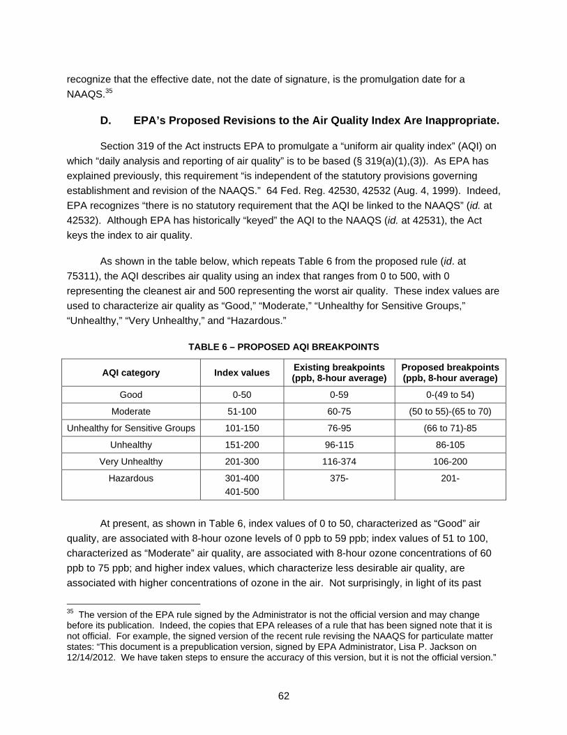
62

recognize that the effective date, not the date of signature, is the promulgation date for a

NAAQS.35

D. EPA’s Proposed Revisions to the Air Quality Index Are Inappropriate.

Section 319 of the Act instructs EPA to promulgate a “uniform air quality index” (AQI) on

which “daily analysis and reporting of air quality” is to be based (§ 319(a)(1),(3)). As EPA has

explained previously, this requirement “is independent of the statutory provisions governing

establishment and revision of the NAAQS.” 64 Fed. Reg. 42530, 42532 (Aug. 4, 1999). Indeed,

EPA recognizes “there is no statutory requirement that the AQI be linked to the NAAQS” (id. at

42532). Although EPA has historically “keyed” the AQI to the NAAQS (id. at 42531), the Act

keys the index to air quality.

As shown in the table below, which repeats Table 6 from the proposed rule (id. at

75311), the AQI describes air quality using an index that ranges from 0 to 500, with 0

representing the cleanest air and 500 representing the worst air quality. These index values are

used to characterize air quality as “Good,” “Moderate,” “Unhealthy for Sensitive Groups,”

“Unhealthy,” “Very Unhealthy,” and “Hazardous.”

TABLE 6 – PROPOSED AQI BREAKPOINTS

AQI category Index values Existing breakpoints (ppb, 8-hour average)

Proposed breakpoints (ppb, 8-hour average)

Good 0-50 0-59 0-(49 to 54)

Moderate 51-100 60-75 (50 to 55)-(65 to 70)

Unhealthy for Sensitive Groups 101-150 76-95 (66 to 71)-85

Unhealthy 151-200 96-115 86-105

Very Unhealthy 201-300 116-374 106-200

Hazardous 301-400

401-500

375- 201-

At present, as shown in Table 6, index values of 0 to 50, characterized as “Good” air

quality, are associated with 8-hour ozone levels of 0 ppb to 59 ppb; index values of 51 to 100,

characterized as “Moderate” air quality, are associated with 8-hour ozone concentrations of 60

ppb to 75 ppb; and higher index values, which characterize less desirable air quality, are

associated with higher concentrations of ozone in the air. Not surprisingly, in light of its past

35 The version of the EPA rule signed by the Administrator is not the official version and may change before its publication. Indeed, the copies that EPA releases of a rule that has been signed note that it is not official. For example, the signed version of the recent rule revising the NAAQS for particulate matter states: “This document is a prepublication version, signed by EPA Administrator, Lisa P. Jackson on 12/14/2012. We have taken steps to ensure the accuracy of this version, but it is not the official version.”

63

focus on keying the AQI to the NAAQS, EPA is proposing to make “confirming changes” to the

AQI, as shown on the table, if it revises the NAAQS. Those changes would lower the ranges of

ozone levels in each category, so that, for example, ozone air quality in the range of 50 or 55

ppb (depending on the level of the revised NAAQS) to 59 ppb would no longer be considered

“Good,” but would be labeled as “Moderate,” and ozone air quality at the level of the current

standard (75 ppb) would be changed from “Moderate” to “Unhealthy for Sensitive Groups.”

These “conforming changes would mean air quality that is actually improving would, in

some instances, be reported as less healthy. An area for which the ozone level improved from

75 ppb to 72 ppb on its most polluted day, for example, would report “Moderate” air quality on

that day under the current AQI. If the AQI were revised as EPA has proposed, however, that

area would be required to report air quality on that day as “Unhealthy for Sensitive Groups,”

thus labeling cleaner air as less healthy. Essentially, the revised AQI would fail to capture air

quality improvements and would suggest degradation in air quality when none has occurred. As

a result, members of the public would likely conclude, erroneously, that air quality had

degraded. Indeed, they might question whether EPA and state regulators were doing their jobs.

Fortunately, there is no requirement that the Agency revise the AQI, leading to such

misleading results. The Act does not require it. As EPA explained previously (64 Fed. Reg. at

42532), the Act does not tie the AQI to NAAQS. Indeed, the purpose of Section 319(a) of the

Act is to provide a consistent, uniform means of gauging air quality. EPA’s proposal to revise

the AQI runs counter to such uniformity. EPA’s proposal would change the air quality

significance of a given index value and its associated AQI category. By contrast, retention of

the current AQI would allow continued provision of uniform information on air quality.

E. EPA Should Not Extend the Ozone Monitoring Season.

EPA’s proposed rule includes a proposal to extend the ozone monitoring season for 33

states from anywhere from one to seven months (79 Fed. Reg. at 75358-60). In describing that

proposal, EPA erroneously refers to days with maximum 8-hour average concentrations above

60 ppb as “exceedance days” (id. at 75358). While EPA states that this threshold is used as

“simply a conservative benchmark that is below the levels proposed for the revised NAAQS”

(id.), these references are clearly misleading to the public. If the Agency uses any ozone

concentration as an indicator of exceedances, that concentration should be the same as the

NAAQS. As previously discussed, the Associations believe that the NAAQS should not be

changed.

In any event,, the Associations oppose any lengthening of the ozone monitoring season

regardless of whether the NAAQS is retained or revised as proposed. The months in which

ozone monitoring is currently required vary from state to state and, for each state, include the

months with conditions most “conducive to ozone formation” based on factors that include

64

temperature, strength of solar insolation, and hours of daylight (id.). Newer science does not

suggest that those considerations are no longer the appropriate ones. Indeed, as EPA

recognizes, ozone concentrations are generally correlated with temperature, with higher

concentrations in warmer months (id. at 75242); and numerous epidemiological studies have

reported stronger associations of ozone concentrations with respiratory effects in the warm

seasons or summer months (id. at 75257 n.54, 75258). Many areas proposed for extended

ozone monitoring seasons have average high temperatures less than 50 degrees Fahrenheit in

the “extended” month(s). Thus, we do not believe that the proposed extensions of the ozone

monitoring season for 33 states is necessary or appropriate. The proposal will needlessly

increase the costs of monitoring by extending the ozone monitoring season while generating

little or no improved health benefits.

F. EPA’s Proposal Does Not Comply with the Federal Information Quality Act.

The federal Data Quality Act, also known as the Information Quality Act (IQA), enacted

as Section 515(a) of the Treasury and General Government Appropriations Act for Fiscal Year

2001 (Public Law 106-554), required federal agencies, such as EPA, to issue guidelines

“ensuring and maximizing the quality, objectivity, utility, and integrity of information . . .

disseminated by the agency.” EPA has issued such guidelines (EPA, 2002). Those guidelines

apply to information disseminated by EPA and establish certain rigorous quality standards for

“influential scientific, financial, or statistical information,” including information that will have a

“clear and substantial impact . . . on important public policies or private sector decisions” (id.)

They require, among other things, that the substance of that information be “accurate, reliable

and unbiased,” including the use of “the best available science and supporting studies

conducted in accordance with sound and objective scientific practices” (id.). The guidelines also

provide mechanisms for challenges to and correction of information that the Agency

disseminates. Clearly, the proposal and adoption of revised NAAQS would qualify as the

dissemination of “influential scientific” information that will have a “clear and substantial impact”

on “important public policies or private sector decisions,” and thus they are subject to the

requirements of the IQA. This is particularly true given the CAA requirement that NAAQS

revisions must “accurately reflect the latest scientific knowledge” (§ 108(a)(2)).

In this case, the Associations submit that EPA’s proposal to revise the NAAQS for ozone

and the associated RIA do not comply with the IQA. The Agency’s proposal is not “accurate,

reliable and unbiased” for many of the reasons discussed in Section III – i.e., that EPA has

failed to properly take account of background concentrations, has failed to adequately explain

its change in interpretations, has failed to take account of the adverse impacts of its proposal,

and has failed to provide an adequate scientific justification for reducing the level of the

standard. As one further example, EPA has not applied an appropriate causal framework, such

65

as that described by Goodman et al. (2013b), in evaluating the health effects data.36 In addition,

EPA’s RIA is not “accurate, reliable and unbiased” for the reasons given in Section IV.

G. EPA Has Not Complied with the Unfunded Mandates Reform Act.

The Unfunded Mandates Reform Act (UMRA) requires that, before promulgating any

notice of proposed rulemaking that is likely to result in the promulgation of a rule that includes a

federal mandate that may result in the expenditure by state or local governments or the private

sector of $100 million in any year, the agency must prepare a written statement that includes,

among other things, an assessment of the costs and benefits of the mandate to the state and

local governments or the private sector, the estimated costs of compliance, and the effect of the

mandate on the national economy (2 U.S.C. § 1532(a)). In its current proposal, EPA dismisses

the requirement to produce such an economic cost analysis under the UMRA on the apparent

ground that EPA cannot consider costs in setting NAAQS (79 Fed. Reg. at 75386).

However, the UMRA requirement to publish a cost analysis is separate from

considerations affecting EPA’s decision on the NAAQS, and, rather, is intended to inform the

public, state and local governments, and Congress regarding the potential that a regulation,

however decided, may have budget implications for state and local governments of which they

need to be aware. A revised ozone NAAQS will inevitably impose costs on the state and local

government entities that must monitor their attainment status and must develop and enforce

policies to attain and maintain compliance. It will also impose economic impacts on private

sector businesses and individual citizens within the affected states, and those economic impacts

on the private sector will likely have further repercussions on state and local governments in

terms of tax revenues and social welfare program expenditures. Even if EPA is correct that the

costs identified under an UMRA analysis cannot affect EPA’s decision on the NAAQS, the

purpose of the UMRA is served by providing credible and good-faith estimates of impacts so

that states are informed to facilitate appropriate budget planning.

An UMRA analysis is also intended to inform Congress, so that legislators may consider

the need to mitigate the identified cost impacts. There is evidence that existing federal funding

to states through grants for air quality monitoring and policy enforcement is inadequate. See

the 2004 report by the State and Territorial Air Pollution Program Administrators and the

Association of Local Air Pollution Control Officials, “The Critical Funding Shortfall of State and

36 We also note that, although EPA no longer places substantial weight on the Harvard Six Cities Study or American Cancer Society-Cancer Prevention Study II, it does rely in part on a recent follow-up from that study (Jerrett et al., 2009); and yet it has failed to provide the underlying data, analysis, and reanalysis of that study after FOIA request by industry, six requests by the House Science, Space, and Technology Committee, and a Congressional subpoena by the House Science, Space and Technology Committee (see http://science.house.gov/sites/republicans.science.house.gov/files/documents/Subpoena%20link.pdf).

66

Local Air Quality Agencies,” at

http://www.4cleanair.org/sites/default/files/Documents/FundingNeedsOverview.pdf. Budget

trends since 2004 have undoubtedly made the funding (or “unfunding”) situation worse. The

delays in compliance with the existing NAAQS promulgated in 2008 are due, in part, to the

effect of existing under-funding of EPA mandates affecting state and local environmental

enforcement agencies, and the additional burden of new ozone NAAQS will only make matters

worse. EPA has a duty under the UMRA to present the facts about the costs of the proposed

changes in the NAAQS so that the affected agencies and Congress will be aware of them and

be able to plan and respond. EPA has not complied with that requirement.37

VI. CONCLUSION

Industry and federal, state, and local regulators are working diligently to implement the

current ozone NAAQS. A further reduction in the level of the NAAQS would impose massive

additional burdens on state and local governments and regulated sources, including the

Associations’ members, and would produce widespread and substantial adverse economic,

social, and energy impacts on all sectors of the U.S. economy, with the risk of bringing

economic growth in many parts of the country to a halt. The imposition of those additional

burdens and impacts is not necessary to protect public health and welfare. In fact, as shown in

this comments, a reduction in the level of the ozone NAAQS as proposed by EPA would be

unlawful under the standard of Section 307(d)(9) of the Act as “arbitrary, capricious, an abuse of

discretion, or otherwise not in accordance with law” and in excess of EPA’s authority under the

Act.

VII. REFERENCES

Note: The references listed below that were not located in EPA Docket ID No. EPA-HQ-OAR-2008-0699 (or an associated docket) or cited in the references in EPA’s proposed rule (79 Fed. Reg. at 75387-95) are marked with asterisks. Those references will be submitted to EPA under separate cover as part of Docket ID No. EPA-HQ-OAR-2008-0699.

Adams, W.C. 2002. Comparison of chamber and face-mask 6.6-hour exposures to ozone on pulmonary function and symptoms response. Inhal. Toxicol. 14: 745-764. Cited in proposed rule.

Adams, W.C. 2006. Comparison of chamber 6.6-h exposures to 0.04-0.08 ppm ozone via square-wave and triangular profiles on pulmonary responses. Inhal. Toxicol. 18: 127-136. Cited in proposed rule.

37 For the same reasons given in the paragraph at the end of Section IV, a full and complete cost assessment under the UMTRA would also need to consider the costs and benefits of the proposed changes in the procedures and requirements for ambient air monitoring and reporting by the states.

67

Air-Conditioning, Heating, and Refrigeration Institute, American Chemistry Council, et al. 2014. Letter to Dr. H. Christopher Frey, Chair, CASAC. March 24. Submitted by National Association of Manufacturers to SAB Staff Office in connection with CASAC review panel meeting on March 25-27, 2014.*

American Chemistry Council, American Forest & Paper Association, American Iron and Steel Institute, American Petroleum Institute, American Wood Council, Corn Refiners Association, Council of Industrial Boiler Owners, National Oilseed Producers Association, Portland Cement Association, Rubber Manufacturers Association, Treated Wood Council, U.S. Chamber of Commerce, and Utility Air Regulatory Group. 2014. Comments on EPA’s Health Risk and Exposure Assessment and Policy Assessment for Ozone. March 20. Docket ID No. EPA-HQ-OAR-2008-0699-0122.

API (American Petroleum Institute). 2014. Projected 8-Hour Ozone Nonattainment Areas. Available at http://api.org/~/media/files/policy/environment/economic-impact-ozone/us-65-2014-1-map.pdf (last visited March 13, 2015).*

Cooper, O.R., D.D. Parrish, A. Stohl, M. Trainer, P. Nédélec, V. Thouret, J.P. Cammas, S.J. Oltmans, B.J. Johnson, D. Tarasick, T. Leblanc, I.S. McDermid, D. Jaffe, R. Gao, J. Stith, T. Ryerson, K. Aikin, T. Campos, A. Weinheimer, and M.A. Avery. 2010. Increasing springtime ozone mixing ratios in the free troposphere over western North America. Nature 463: 344-348.*

Electric Power Research Institute (EPRI). 2015. Comments of the Electric Power Research Institute on Environmental Protection Agency’s proposed rule on National Ambient Air Quality Standards for Ozone. Submitted to EPA Docket ID No. EPA-HQ-OAR-2008-0699. March 5.

EPA. 2002. Guidelines for Ensuring and Maximizing the Quality, Objectivity, Utility, and Integrity of Information Disseminated by the Environmental Protection Agency. EPA/260R-02-008. October.*

EPA. 2013. Integrated Science Assessment for Ozone and Related Photochemical Oxidants. National Center for Environmental Assessment-RTP Division, Office of Research and Development, U.S. Environmental Protection Agency. EPA/600/R-10/076F. February. Docket ID No. EPA-HQ-OAR-2008-0699-0405.

EPA. 2014a. Health Risk and Exposure Assessment for Ozone, Final Report. Office of Air Quality Standards and Planning, Health and Environmental Impacts Division, U.S. Environmental Protection Agency. EPA-452/R-14-004a. August. Docket ID No. EPA-HQ-OAR-2008-0699-0233.

EPA. 2014b. Welfare Risk and Exposure Assessment for Ozone, Final. Office of Air Quality Standards and Planning, Health and Environmental Impacts Division, U.S. Environmental Protection Agency. EPA-452/R-14-005a. August. Docket ID No. EPA-HQ-OAR-2008-0699-0234.

68

EPA. 2014c. Policy Assessment for the Review of the Ozone National Ambient Air Quality Standards. Office of Air Quality Standards and Planning, Health and Environmental Impacts Division, U.S. Environmental Protection Agency. EPA-452/R-14-006. August. Docket ID No. EPA-HQ-OAR-2008-0699-0404.

EPA. 2014d. Regulatory Impact Analysis of the Proposed Revisions to the National Ambient Air Quality Standards for Ground-Level Ozone. Office of Air Quality Standards and Planning, U.S. Environmental Protection Agency. EPA-452/P-14-006. November. Docket ID No. EPA-HQ-OAR-2013-0169.

EPA. 2015. 8-Hour Ozone Nonattainment Areas (2008 Standard). Available at http://www.epa.gov/airquality/greenbk/map8hr_2008.html (last visited March 13, 2015).

Frey, H.C. 2014. Letter from CASAC Chairman H. Christopher Frey to EPA Administrator Gina McCarthy; CASAC Review of the EPA’s Second Draft Policy Assessment for the Review of the Ozone National Ambient Air Quality Standards. June 26. Cited in proposed rule.

Goodman, J.E., R.L. Prueitt, J. Chandalia, and S.J. Sax. 2013a. Evaluation of adverse human lung function effects in controlled ozone exposure studies. J. Appl. Toxicol. doi: 10.1002/jat.2905.*

Goodman, J.E., R.L. Prueitt, S.N. Sax, L.A. Bailey, and L.R. Rhomberg. 2013b. Evaluation of the causal framework for setting National Ambient Air Quality Standards. Crit. Rev. Toxicol. 43: 829-149.*

Goodman, J.E., and S.N. Sax. 2014a. Letter to Dr. H. Christopher Frey, Chair, CASAC. March 13. Submitted to SAB Staff Office in connection with CASAC review panel meeting on March 25-27, 2014.*

Goodman, J.E., and S. Sax. 2014b. Comments on the CASAC Review of the Health Risk and Exposure Assessment and the Policy Assessment for Ozone. Memorandum submitted to CASAC. May 14.*

Goodman, J.E., M. Seeley, R. Mattuck, and S. Thakali. 2015. Do group responses mask the effects of air pollutants on potentially sensitive individuals in controlled human exposure studies? Reg. Toxicol. Pharmacol., in press. Submitted to EPA by Gradient on February 11, 2015 . Docket ID No. EPA-HQ-OAR-2008-0699-1127.

Gradient. 2013a. Long-Term Ozone Exposure and Mortality. Prepared for Utility Air Regulatory Group. April 26. Attachment to above-cited comments of American Chemistry Council et al. (2014). Docket ID No. EPA-HQ-OAR-2008-0699-0122.

Gradient. 2013b. Short-Term Ozone Exposure and Mortality. Prepared for Utility Air Regulatory Group. December 20. Attachment to above-cited comments of American Chemistry Council et al. (2014). Docket ID No. EPA-HQ-OAR-2008-0699-0122.

69

Gradient. 2013c. Long-Term Ozone Exposure and Respiratory Morbidity. Prepared for Utility Air Regulatory Group. December 20. Attachment to above-cited comments of American Chemistry Council et al. (2014). Docket ID No. EPA-HQ-OAR-2008-0699-0122.

Gradient. 2014. Comments on the Secondary Standard for Ozone and Related Photochemical Oxidants. Prepared for the Utility Air Regulatory Group. Attached to below-cited comments of the Utility Air Regulatory Group (2014). Docket ID No. EPA-HQ-OAR-2008-0699-0129.

Gradient. 2015. Comments on the National Ambient Air Quality Standards for Ozone Proposed Rule. March 16, 2015. Submitted to Docket ID No. EPA-HQ-OAR-2008-0699.

Grulke, N.E., R.A. Minnich, T.D. Paine, S.J. Seybold, D.J. Chavez, M.E. Fenn, P.J. Riggin, and A. Dunn. 2008. Air pollution increases forest susceptibility to wildfires: A case study in the San Bernardino Mountains in southern California. In A. Bytnerowicz et al. (eds.), 2009, Wildland Fires and Air Pollution; Section III: Ecological Impacts of Forest Fires and Air Pollution (pp. 365-403). Amsterdam, The Netherlands, Elsevier Ltd.*

Hatch, O., M. Lee, R. Bishop, J. Chaffretz, and C. Stewart. 2014. Letter to Hon. Gina McCarthy, Administrator, U.S. Environmental Protection Agency. November 25. Docket ID No. EPA-HQ-OAR-2008-0699-0351.

Heuss, J.M., and G.T. Wolff. 2012. Review and Critique of the U.S. Environmental Protection Agency’s Third External Review Draft of the “Integrated Science Assessment for Ozone and Related Photochemical Oxidants.” Prepared for The Alliance of Automobile Manufacturers. August 20. Submitted to SAB Staff Office in connection with CASAC review panel meeting on September 11-13, 2012.*

Heuss, J.M., G.T. Wolff, and D.F. Kahlbaum. 2014. Review and Critique of the U.S. Environmental Protection Agency Second External Review Drafts of the “Health Risk and Exposure Assessment for Ozone” and the “Policy Assessment for the Review of the Ozone National Ambient Air Quality Standards.” Prepared for The Alliance of Automobile Manufacturers. March 24. Submitted to SAB Staff Office in connection with CASAC review panel meeting on March 25-27, 2014. Docket ID No. EPA-HQ-OAR-2008-0699-0135.

Jerrett, M., R.T. Burnett, C.A. Pope III, K. Ito, G. Thurston, D. Krewski, Y. Shi, E. Calle, and M. Thun. 2009. Long-term ozone exposure and mortality. N. Engl. J. Med. 360: 1085-1095. Cited in proposed rule.

Kaiser, C. 2014. Letter to Dr. Christopher Frey, Chair, CASAC. March 24. Prepared for Kennecott Utah Copper LLC. Submitted to SAB Staff Office in connection with CASAC review panel meeting on March 25-27, 2014. Docket ID No. EPA-HQ-OAR-2008-0699-0130.

Kim, C.S., N.E. Alexis, A.G. Rappold, H. Kehrl, M.J. Hazucha, J.C. Lay, M.T. Schmitt, M. Case, R.B. Devlin, D.B. Peden, and D. Diaz-Sanchez. 2011. Lung function and inflammatory responses in healthy young adults exposed to 0.06 ppm ozone for 6.6 hours. Am. J. Respir. Crit. Care Med. 183: 1215-1221. Cited in proposed rule.

70

Langford, A.O., C.J. Senff, R.J. Alvarez II, J. Brioude, O.R. Cooper, J.S. Holloway, M.Y. Lin, R.D. Marchbanks, R.B. Pierce, S.P. Sandberg, A.M. Weickmann, and E.J. Williams. 2014. An overview of the 2013 Las Vegas Ozone Study (LVOS): Impact of stratospheric intrusions and long-range transport on surface air quality. Atmos. Environ. XX (2014): 1-18, http://dx.doi.org/10.1016/j.atmosenv.2014.08.040.*

Lefohn, A.S., and S.J. Oltmans. 2012. Background Ozone and Its Importance in Relation to the Health Risk and Exposure Assessment for Ozone Assessment Document. September 18. Docket ID No. EPA-HQ-OAR-2008-0699-0090.

Lefohn, A.S., and S.J. Oltmans. 2014. Background Ozone and Its Importance in Relation to the Health Risk and Exposure Assessment for Ozone Assessment Document. March 13. Submitted to SAB Staff Office in connection with CASAC review panel meeting on March 25-27, 2014. Docket ID No. EPA-HQ-OAR-2008-0699-0118.

Lefohn, A.S., H. Wernli, D. Shadwick, S.J. Oltmans, and M. Shapiro. 2012. Quantifying the importance of stratospheric-tropospheric transport on surface ozone concentrations at high- and low-elevation monitoring sites in the United States. Atmos. Environ. 62 (2012): 646-656.*

Lefohn, A.S., C. Emery, D. Shadwick, H. Wernli, J. Jung, and S.J. Oltmans. 2014. Estimates of background surface ozone concentrations in the United States based on model-derived source apportionment. Atmos. Environ. 84 (2014): 276-288.*

Mar, T.F., and J.Q. Koenig. 2009. Relationship between visits to emergency departments for asthma and ozone exposure in greater Seattle, Washington. Ann. Allergy Asthma Immunol. 103: 474-479. Cited in proposed rule.

McCarthy, G. 2012. Letter from Gina McCarthy, Assistant Administrator, to Robert Ukeiley regrading petition on behalf of Sierra Club (Jan. 4, 2012). Available at http://www.epa.gov/scram001/10thmodcong/review_material/Sierra_Club_Petition_OAR-11-002-1093.pdf. Docket ID No. EPA-HQ-OAR-2008-0699-0304.

Page, S.D., 2013. Interim Guidance to Implement Requirements for the Treatment of Air Quality Monitoring Data Influenced by Exceptional Events. Memorandum from Director, Office of Air Quality Planning and Standards, EPA, to Regional Air Directors. May 10. Available at http://www.epa.gov/ttn/analysis/exevents.htm. Docket ID No. EPA-HQ-OAR-2008-0699-0235.

Schelegle, E.S., C.A. Morales, W.F. Walby, S. Marion, and R.P. Allen. 2009. 6.6-hour inhalation of ozone concentrations from 60 to 87 parts per billion in healthy humans. Am. J. Respir. Crit. Care Med. 180: 265- 272. Cited in proposed rule.

Smith, A. 2013. Testimony of Amanda Smith, Executive Director, Utah Department of Environmental Quality, before the Sub-Committee on Environment of the Committee on Science, Space and Technology. June 12.*

71

Utility Air Regulatory Group (UARG). 2012. Comments of the Utility Air Regulatory Group on the Third Draft Integrated Science Assessment. Submitted to Docket No. EPA-HQ-ORD-2011-0050. August 20. Docket ID No. EPA-HQ-ORD-2011-0050-0046.

Utility Air Regulatory Group (UARG). 2014. Comments of the Utility Air Regulatory Group on the U.S. Environmental Protection Agency’s Health Risk and Exposure Assessment for Ozone: Second External Review Draft (February 2014) and Welfare Risk and Exposure Assessment for Ozone: Second External Review Draft (February 2014) and Policy Assessment for the Review of the National Ambient Air Quality Standards: Second External Review Draft (January 2014). March 24. Docket ID No. EPA-HQ-OAR-2008-0699-0129.

Wells, B. 2014. Comparison of Ozone Metrics Considered in Current NAAQS Review. Memorandum to the Ozone NAAQS Review Docket. Docket ID No. EPA-HQ-OAR-2008-0699-0155.

Wittig, V.E., E.A. Ainsworth, S.L. Naidu, D.F. Karnosky, and S.P Long. 2009. Quantifying the impact of current and future tropospheric ozone on tree biomass, growth, physiology, and biochemistry: A quantitative meta-analysis. Global Change Biol. 15: 396-424. Cited in proposed rule.

Wolff, G.T., J.M. Heuss, and D. Kahlbaum. 2014. Comments on Background Ozone Related to the Review of the Secondary Ozone NAAQS As Discussed in the Second Draft of EPA’s Policy Assessment and Welfare REA. Prepared for The Utility Air Regulatory Group and The Alliance of Automobile Manufacturers. March 24. Submitted to SAB Staff Office in connection with CASAC review panel meeting on March 25-27, 2014. Docket ID No. EPA-HQ-OAR-2008-0699-0129.

Zhang, L., D.J. Jacob, N.V. Downey, D.A. Wood, D. Blewitt, C.C. Carouge, A. van Donkelaar, D.B.A. Jones, L.T. Murray, and Y. Yang. 2011. Improved estimate of the policy-relevant background ozone in the United States using the GEOS-Chem global model with 1/2º x 2/3º horizontal resolution over North America. Atmos. Environ. 45: 6769-6775, http://dx.doi.org/10.1016/j.atmosenv.2011.07.054.*

ATTACHMENT A

BRAC Public Policy Commentary:

Eighteen of Twenty Top-Performing Metro Economies at Risk from New Ozone Standards

Published on Monday, March 2, 2015

All but two of the nation’s top twenty metropolitan area economies, as ranked by the Brookings Institution’s assessment of performance through recession and recovery, would fall into “ozone nonattainment” status if the Obama administration moves forward with its more aggressive regulatory plans for air quality, according to an analysis completed by the Baton Rouge Area Chamber (BRAC) The proposed National Ambient Air Quality Standards (NAAQS) for ground level ozone rule, issued by the Environmental Protection Agency (EPA) on December 17, 2014, is designed to lower the current NAAQS of seventy-five parts-per-billion (ppb) to a range between sixty-five and seventy ppb. Should the Obama administration push forward with a standard of sixty-five ppb, eighteen of the U.S.’s twenty top-performing metropolitan economies would find themselves in a regulatory posture of “nonattainment,” and all the regulatory consequences that entails.

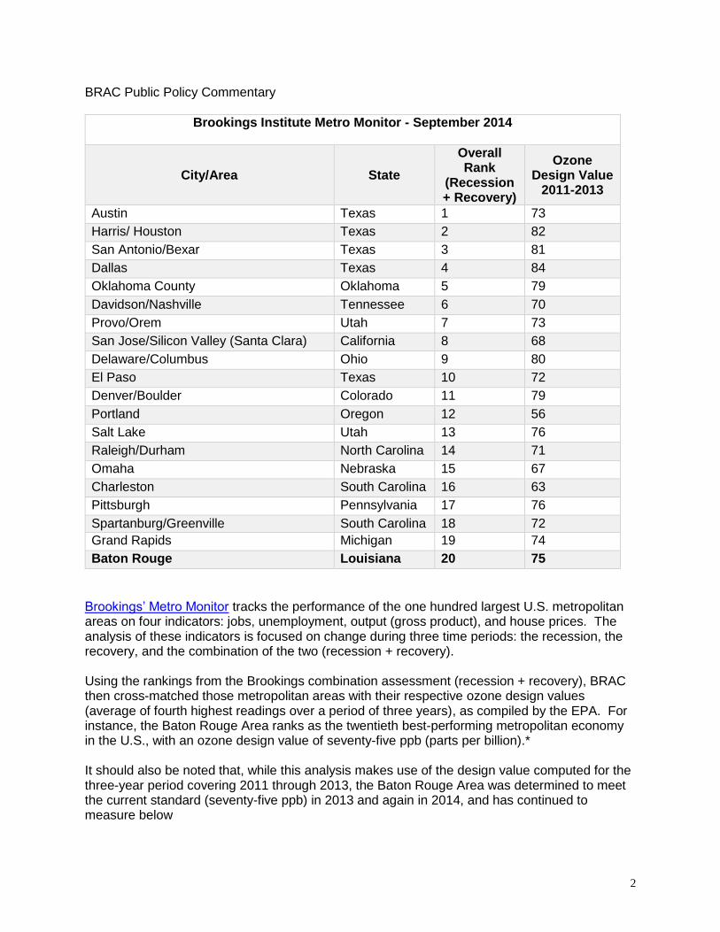
2

BRAC Public Policy Commentary

Brookings Institute Metro Monitor - September 2014

City/Area State

Overall Rank

(Recession + Recovery)

Ozone Design Value

2011-2013

Austin Texas 1 73

Harris/ Houston Texas 2 82

San Antonio/Bexar Texas 3 81

Dallas Texas 4 84

Oklahoma County Oklahoma 5 79

Davidson/Nashville Tennessee 6 70

Provo/Orem Utah 7 73

San Jose/Silicon Valley (Santa Clara) California 8 68

Delaware/Columbus Ohio 9 80

El Paso Texas 10 72

Denver/Boulder Colorado 11 79

Portland Oregon 12 56

Salt Lake Utah 13 76

Raleigh/Durham North Carolina 14 71

Omaha Nebraska 15 67

Charleston South Carolina 16 63

Pittsburgh Pennsylvania 17 76

Spartanburg/Greenville South Carolina 18 72 Grand Rapids Michigan 19 74 Baton Rouge Louisiana 20 75

Brookings’ Metro Monitor tracks the performance of the one hundred largest U.S. metropolitan areas on four indicators: jobs, unemployment, output (gross product), and house prices. The analysis of these indicators is focused on change during three time periods: the recession, the recovery, and the combination of the two (recession + recovery). Using the rankings from the Brookings combination assessment (recession + recovery), BRAC then cross-matched those metropolitan areas with their respective ozone design values (average of fourth highest readings over a period of three years), as compiled by the EPA. For instance, the Baton Rouge Area ranks as the twentieth best-performing metropolitan economy in the U.S., with an ozone design value of seventy-five ppb (parts per billion).* It should also be noted that, while this analysis makes use of the design value computed for the three-year period covering 2011 through 2013, the Baton Rouge Area was determined to meet the current standard (seventy-five ppb) in 2013 and again in 2014, and has continued to measure below

3

BRAC Public Policy Commentary seventy-five ppb throughout its statistical area. Yet while the Baton Rouge Area continues to make this positive environmental progress, it also has firsthand experience with what it means to be in nonattainment – a status that could soon apply to almost all other top-performing metros. A report published by the National Association of Manufacturers in July 2014 assessed the potential economic impact of the proposed new ozone standards, but it also touched upon what “nonattainment” means in practical terms. As the report explained:

“The greatest costs to comply with ozone regulations generally occur in nonattainment areas. The consequences for nonattainment are severe and can include a loss of industry and economic development resulting from increased costs, delays and uncertainties from restrictive permitting requirements; loss of federal highway and transit funding; requirements that any new emissions in the area be offset or the facility cannot be built; and technical and formula changes for commercial and consumer products.”

Mary Martin, who serves as Energy, Clean Air and Natural Resources Policy counsel for the U.S. Chamber, has described how these restrictions translate into consequences:

“[F]ailure to comply with existing ozone standards can lead to non-attainment designation, which are often viewed as a death knell for economic and business development in an area.

“Indeed, severe repercussion[s] result almost immediately from non-attainment designation, such as increased costs to industry, permitting delays, restrictions on expansion, as well as impacts to transportation planning. There are significant adverse consequences to being designated a non-attainment area, making it substantially harder for a community to attract new business or expand existing facilities. Furthermore, in non-attainment areas, EPA is able to revise existing air permits, which can cause tremendous uncertainty, delays, and increased costs in the permitting process for businesses.”

While the Baton Rouge Area Chamber believes in and stands for cleaner air and an improved environment, it continues to vehemently oppose the proposed reductions in ambient air quality standards from the current level of seventy-five ppb. Since the EPA first proposed lowering the ozone standard in December, the Baton Rouge Area has seen four major industrial projects totaling 2,000 direct and indirect jobs, and more than $7 billion in capital investment, either put on hold or redirected elsewhere. These losses are in direct correlation with the uncertainty created by the newly proposed ozone standards rule. The direct impact on the Baton Rouge Area, in terms of new payroll created from the projects themselves, would have been over $86 million annually in wages for the local economy. Also, because these projects included foreign direct investment projects, they also represented new investment from multi-national corporations into the country. Federal regulations concerning NAAQS are having a direct, negative effect on competing U.S. goals for increasing foreign direct investment and exports.

4

BRAC Public Policy Commentary In the Baton Rouge Area case outlined above, these consequences came about merely from the regulation being proposed. Imagine the losses if it is actually implemented, losses not only for Baton Rouge but for other top-performing metros across the country. The implication is that U.S. government policy toward ozone, as proposed, runs in direct contradiction to America's economic goals. More time should be taken to plan solutions that avoid the negative effects on the national economy, and especially on the top-performing regional economies in the United States. *EPA recommends using the Core Based Statistical Area (CBSA) as the starting point to determine boundaries of ozone nonattainment. Based on this approach the highest monitored value of ozone in a CBSA was provided.

About the Baton Rouge Area Chamber The Baton Rouge Area Chamber (BRAC) leads economic development in the nine-parish Baton Rouge Area, working to attract new companies and assisting existing companies with growth and expansions. Today, BRAC investors include more than 1,300 businesses, civic organizations, education institutions, and individuals. In this capacity, BRAC serves as the voice of the business community, providing knowledge, access, services, and advocacy. More information is available at www.brac.org. For more information, contact: Lauren Hatcher Director, Marketing Operations Baton Rouge Area Chamber 225-381-7132 lauren@brac.org

ATTACHMENT B

Economic Impacts of a 65 ppb National Ambient

Air Quality Standard for Ozone

Executive Summary

Prepared for:

National Association of Manufacturers

February 2015

pPro

NERA Economic Consulting

Project Directors

David Harrison, Jr., Ph.D.

Anne E. Smith, Ph.D.

Project Team

Scott Bloomberg

Sugandha Tuladhar, Ph.D.

Andrew Stuntz

Conor Coughlin

Julia Greenberger

Carl McPherson

Christopher D’Angelo

Mei Yuan, Ph.D.

NERA Economic Consulting

200 Clarendon St, 11th Floor

Boston, Massachusetts 02116 Tel: +1 617 927 4500

Fax: +1 617 927 4501

1255 23rd St, NW, Suite 600

Washington, D.C. 20037

Tel: +1 202 466 3510 Fax: +1 202 466 3605

www.nera.com

pPro

NERA Economic Consulting

Report Qualifications/Assumptions and Limiting Conditions

Information furnished by others, upon which all or portions of this report are based, is believed

to be reliable, but has not been independently verified, unless otherwise expressly indicated.

Public information and industry and statistical data are from sources we deem to be reliable;

however, we make no representation as to the accuracy or completeness of such information.

The findings contained in this report may contain predictions based on current data and historical

trends. Any such predictions are subject to inherent risks and uncertainties. NERA Economic

Consulting accepts no responsibility for actual results or future events.

The opinions expressed in this report are valid only for the purpose stated herein and as of the

date of this report. No obligation is assumed to revise this report to reflect changes, events or

conditions, which occur subsequent to the date hereof. The opinions expressed in this report are

those of the authors and do not necessarily represent the views of NERA Economic Consulting,

other NERA consultants, or NERA’s clients.

All decisions in connection with the implementation or use of advice or recommendations

contained in this report are the sole responsibility of the client. This report does not represent

investment advice nor does it provide an opinion regarding the fairness of any transaction to any

and all parties.

pPro

NERA Economic Consulting

S-1

EXECUTIVE SUMMARY

This study evaluates the potential compliance costs and impacts on the U.S. economy if the U.S.

Environmental Protection Agency (EPA) were to set a National Ambient Air Quality Standard

(NAAQS) for ozone of 65 parts per billion (ppb). Employing our integrated energy-economic

macroeconomic model (NewERA), we estimate that the potential emissions control costs could

reduce U.S. Gross Domestic Product (GDP) by about $140 billion per year on average over the

period from 2017 through 2040 and by about $1.7 trillion over that period in present value

terms.1 The potential labor market impacts represent an average annual loss employment income

equivalent to 1.4 million jobs (i.e., job-equivalents).2

These results represent updated values from the results in our July 2014 report (NERA 2014),

which developed estimates of the potential costs and economic impacts of achieving a 60 ppb

ozone standard using the best information then available. In November 2014, the U.S.

Environmental Protection Agency (EPA) released updated emissions and cost information

supporting their proposal to revise the ozone standard (EPA 2014a); we have used that new

information to update our analysis. Also, given that the proposed rule suggests setting a revised

ozone NAAQS in the range of 65 ppb to 70 ppb, in this update we assess the economic impacts

of a potential 65 ppb ozone NAAQS. This Executive Summary of our study begins with a

summary of the differences between the information and methodology in our July 2014 report

and those used in this updated study. It then provides summaries of our estimates of the costs

and economic impacts of attaining a potential ozone NAAQS of 65 ppb.

Changes in Data and Methodology Since the July 2014 Report

The methodology used for this study is largely similar to the methodology used in our July 2014

report. This section discusses changes to the three components of our analysis:

1. The methodology for estimating emission reductions. This study used updated EPA

information on the future NOX and VOC emissions levels needed to comply with a

potential 65 ppb standard (rather than a 60 ppb standard as in our July 2014 report).

1 All dollar values in this report are in 2014 dollars unless otherwise noted. The present value reflects impacts from

2017 through 2040, as of 2014 discounted at a 5% real discount rate; this discount rate falls in the 3% to 7% range

recommended in EPA’s Guidelines for Preparing Economic Analyses (2010a, p. 6-19), and it is consistent with the

discount rate used in the NewERA model.

2 “Job-equivalents” is defined as total labor income change divided by the average annual income per job. This

measure does not represent a projection of numbers of workers that may need to change jobs and/or be

unemployed, as some or all of the loss could be spread across workers who remain employed, thereby impacting

many more that 1.4 million workers, but with lesser impacts per worker.

pPro

NERA Economic Consulting

S-2

Additionally, we used updated cost and effectiveness information about emission controls

that have been identified by EPA.

2. The methodology for estimating compliance costs. We updated the costs of the known

controls that EPA identified to attain the 65 ppb standard using EPA’s new cost data.

However, even for a 65 ppb standard, more than half of the emissions reductions needed

across the country would come from measures that EPA still has not identified. Using

the same evidence-based approach for developing a cost curve that we used in our July

analysis (but using the more recent inventory data, and updating the calculations for a

later year of compliance spending), we calculated the costs of the set of further emissions

reduction needs that EPA has left unidentified in its current analysis. We also updated all

dollar figures from 2013 to 2014 dollars.

3. The methodology for estimating economic impacts. We used the same version of

NERA’s NewERA macroeconomic model as our previous study to estimate the economic

impacts of our estimated costs for reducing emissions in the amount necessary to attain a

65 ppb ozone standard. In contrast to EPA’s analysis, we excluded the proposed EPA

Clean Power Plan rule from our modeling baseline.

In our July 2014 report, we performed a sensitivity analysis on the possibility that nonattainment,

especially in rural areas of the U.S., could create barriers to continued growth in oil and gas

extraction. A national policy question that remains in a state of flux is whether or not new

permitting requirements hinder growth in energy production. A tightened ozone standard has the

potential to cause nonattainment areas to expand into relatively rural areas, where there are few

or no existing emissions sources that could be controlled to offset increased emissions from new

activity. If nonattainment expands into rural areas that are active in U.S. oil and gas extraction, a

shortage of potential offsets may translate into a significant barrier to obtaining permits for the

new wells and pipelines needed to expand (or even maintain) our domestic oil and gas

production levels. The sensitivity analysis in our July 2014 report resulted in much larger natural

gas price effects, and raised macroeconomic impacts of our base case by about 30 to 50%.

Limitations of time have prevented us from conducting a similar sensitivity analysis for this

update.

Methodology for Estimating Emission Reductions

The July 2014 report relied on projected 2018 baseline VOC and NOX emissions and EPA

information from its 2008 and 2010 Regulatory Impact Analyses (RIAs) to estimate reductions

required for all regions of the U.S. to come into compliance with a 60 ppb standard. The updated

EPA information that we rely on in this study includes projected 2018 and 2025 base case and

baseline emissions as well as EPA’s estimates of reductions required from the 2025 baseline

emissions to achieve a 65 ppb standard (EPA 2014a-g). We use the updated EPA estimates of

pPro

NERA Economic Consulting

S-3

state-by-state emissions reductions from the 2025 baseline as the principal basis for our estimates

of NOX emissions levels that would allow a 65 ppb standard to be attained nationwide.3 In order

to reach and maintain this level of NOX emissions consistent with a 65 ppb ozone concentration,

states would need to reduce emissions at existing sources and prevent any net increases in

emissions from new or expanded sources. We also rely on EPA’s revised data on the cost of

emissions reductions for “known” control measures, which are provided by source sector and

state.

Our methodology for estimating costs of emission reductions is similar to our July 2014 study. In

both studies, we substituted our base case estimates of electricity generating unit (EGU)

emissions for those of EPA, for consistency with our economic impact model, which estimates

costs from EGU emissions reductions endogenously. As before, we adopted EPA’s cost

estimates for those controls that EPA identifies as “known”—that is specific controls for which

EPA had developed emission reduction and cost information—and we applied our own more

evidence-based approach for estimating costs for the many required reductions that EPA treats as

“unknown.” For estimating the impacts to the U.S. economy of our estimates of compliance

costs, we assigned each state’s projected cost to specific calendar years, using assessments of

their likely attainment dates. Also consistent with our prior study, we assigned the costs to

specific sectors in each state; for the “known” control measures these assignments were based on

the sector-specific information available in EPA’s data and for the “unknown” control measures,

these assignments were based on emissions inventory data on the relative contribution of each

source category to the remaining emissions in each state.

Methodology for Estimating Compliance Costs

Our methodology for developing estimates of compliance costs in this study is the same as in our

July 2014 report, although of course the numerical values are different reflecting the additional

information now available. As noted, EPA developed updated estimates of the annualized costs

from “known” controls, and we used this updated information on “known” controls.

As in the July 2014 analysis, emission reductions from “known” controls were not sufficient to

achieve attainment, in this case with a 65 ppb ozone standard. EPA has filled the gap with a

rough estimate of costs of “unknown” controls, i.e., controls for which no cost information was

developed. In contrast to the two cost estimation methodologies presented in its 2008 and 2010

RIAs, this time EPA used a single simplistic assumption that annualized control costs for these

“unknown” controls would be equal to $15,000 per ton, regardless of the state, the sector, or the

amount of emission reduction required. This estimate was not based upon any evidence-based

3 We focused our analysis on NOX emissions, but we also included EPA’s estimates of VOC emission control costs

in our modeling.

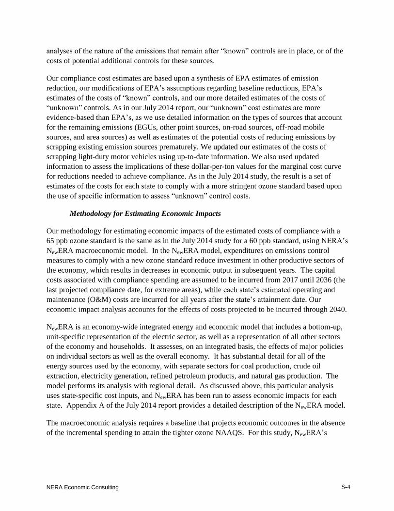
pPro

NERA Economic Consulting

S-4

analyses of the nature of the emissions that remain after “known” controls are in place, or of the

costs of potential additional controls for these sources.

Our compliance cost estimates are based upon a synthesis of EPA estimates of emission

reduction, our modifications of EPA’s assumptions regarding baseline reductions, EPA’s

estimates of the costs of “known” controls, and our more detailed estimates of the costs of

“unknown” controls. As in our July 2014 report, our “unknown” cost estimates are more

evidence-based than EPA’s, as we use detailed information on the types of sources that account

for the remaining emissions (EGUs, other point sources, on-road sources, off-road mobile

sources, and area sources) as well as estimates of the potential costs of reducing emissions by

scrapping existing emission sources prematurely. We updated our estimates of the costs of

scrapping light-duty motor vehicles using up-to-date information. We also used updated

information to assess the implications of these dollar-per-ton values for the marginal cost curve

for reductions needed to achieve compliance. As in the July 2014 study, the result is a set of

estimates of the costs for each state to comply with a more stringent ozone standard based upon

the use of specific information to assess “unknown” control costs.

Methodology for Estimating Economic Impacts

Our methodology for estimating economic impacts of the estimated costs of compliance with a

65 ppb ozone standard is the same as in the July 2014 study for a 60 ppb standard, using NERA’s

NewERA macroeconomic model. In the NewERA model, expenditures on emissions control

measures to comply with a new ozone standard reduce investment in other productive sectors of

the economy, which results in decreases in economic output in subsequent years. The capital

costs associated with compliance spending are assumed to be incurred from 2017 until 2036 (the

last projected compliance date, for extreme areas), while each state’s estimated operating and

maintenance (O&M) costs are incurred for all years after the state’s attainment date. Our

economic impact analysis accounts for the effects of costs projected to be incurred through 2040.

NewERA is an economy-wide integrated energy and economic model that includes a bottom-up,

unit-specific representation of the electric sector, as well as a representation of all other sectors

of the economy and households. It assesses, on an integrated basis, the effects of major policies

on individual sectors as well as the overall economy. It has substantial detail for all of the

energy sources used by the economy, with separate sectors for coal production, crude oil

extraction, electricity generation, refined petroleum products, and natural gas production. The

model performs its analysis with regional detail. As discussed above, this particular analysis

uses state-specific cost inputs, and NewERA has been run to assess economic impacts for each

state. Appendix A of the July 2014 report provides a detailed description of the NewERA model.

The macroeconomic analysis requires a baseline that projects economic outcomes in the absence

of the incremental spending to attain the tighter ozone NAAQS. For this study, NewERA’s

pPro

NERA Economic Consulting

S-5

baseline conditions were calibrated to reflect projections developed by Federal government

agencies, notably the Energy Information Administration (EIA) as defined in its Annual Energy

Outlook 2014 (AEO 2014) Reference case. This baseline includes the effects of environmental

regulations that have already been promulgated as well as other factors that lead to changes over

time in the U.S. economy and the various sectors. Our baseline does not include the effects of

proposed regulations, such as the Clean Power Plan (CPP), although we do include power sector

closures as an available way to attain the NAAQS, to the extent that we find such closures to be

cost-effective elements of each state’s control strategy.4

The July 2014 report and appendices provide details on the various aspects of our methodology,

subject to the changes noted above. Although this Executive Summary report describes results

for the United States as a whole and disaggregated to 11 regions,5 the inputs and the results are

built up using detailed state-specific and sector-specific cost information. The costs and impacts

of a more stringent ozone standard differ substantially among states.

Summary of National Results

Emission Reductions Required to Achieve a 65 ppb Ozone Standard

As Figure S-1 illustrates, national NOX emissions have already been reduced substantially, from

about 25.2 million tons in 1990 to 12.9 million tons in 2013 (EPA 2014b). EPA currently

projects that U.S. NOX emissions will be further reduced by existing rules and regulations to 8.2

million tons by 2025 (supplemented with NewERA’s projected baseline EGU emissions, which

does not include the proposed CPP). Those additional emissions reductions between 2013 and

2025 will involve costs beyond the compliance costs estimated in this study. Economic activity

(as measured by real GDP) in 2025 is projected to be more than double the level in 1990 (CEA

2014, Table B-3 and OMB 2013, Table 2), suggesting that U.S. NOX sources will have been

controlled by more than 80% by 2025, without the additional controls needed to attain a tighter

ozone NAAQS.

4 EPA’s inclusion of the CPP in its baseline was inconsistent with its standard practice of only including

promulgated regulations. This deviation from standard procedure seems particularly unjustified given the enormous

uncertainty in what carbon limits may actually be applied and how states would comply, and hence what NOX

emission reductions might actually occur as a result of this carbon regulation.

5 “U.S.” results are, formally, only for the lower 48 states, and exclude Alaska and Hawaii, as well as Washington

DC. We refer to the lower 48 states as “U.S.” hereafter.

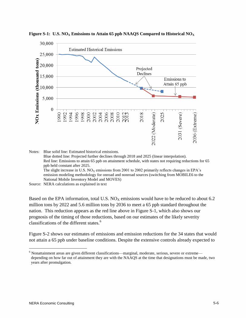
pPro

NERA Economic Consulting

S-6

Based on the EPA information, total U.S. NOX emissions would have to be reduced to about 6.2

million tons by 2022 and 5.6 million tons by 2036 to meet a 65 ppb standard throughout the

nation. This reduction appears as the red line above in Figure S-1, which also shows our

prognosis of the timing of those reductions, based on our estimates of the likely severity

classifications of the different states.6

Figure S-2 shows our estimates of emissions and emission reductions for the 34 states that would

not attain a 65 ppb under baseline conditions. Despite the extensive controls already expected to

6 Nonattainment areas are given different classifications—marginal, moderate, serious, severe or extreme—

depending on how far out of attainment they are with the NAAQS at the time that designations must be made, two

years after promulgation.

Figure S-1: U.S. NOX Emissions to Attain 65 ppb NAAQS Compared to Historical NOX

Notes: Blue solid line: Estimated historical emissions.

Blue dotted line: Projected further declines through 2018 and 2025 (linear interpolation).

Red line: Emissions to attain 65 ppb on attainment schedule, with states not requiring reductions for 65

ppb held constant after 2025.

The slight increase in U.S. NOX emissions from 2001 to 2002 primarily reflects changes in EPA’s

emission modeling methodology for onroad and nonroad sources (switching from MOBILE6 to the

National Mobile Inventory Model and MOVES)

Source: NERA calculations as explained in text

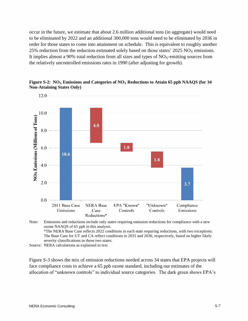
pPro

NERA Economic Consulting

S-7

occur in the future, we estimate that about 2.6 million additional tons (in aggregate) would need

to be eliminated by 2022 and an additional 300,000 tons would need to be eliminated by 2036 in

order for those states to come into attainment on schedule. This is equivalent to roughly another

25% reduction from the reduction estimated solely based on those states’ 2025 NOX emissions.

It implies almost a 90% total reduction from all sizes and types of NOX-emitting sources from

the relatively uncontrolled emissions rates in 1990 (after adjusting for growth).

Figure S-3 shows the mix of emission reductions needed across 34 states that EPA projects will

face compliance costs to achieve a 65 ppb ozone standard, including our estimates of the

allocation of “unknown controls” to individual source categories. The dark green shows EPA’s

Figure S-2: NOX Emissions and Categories of NOX Reductions to Attain 65 ppb NAAQS (for 34

Non-Attaining States Only)

Note: Emissions and reductions include only states requiring emission reductions for compliance with a new

ozone NAAQS of 65 ppb in this analysis.

*The NERA Base Case reflects 2022 conditions in each state requiring reductions, with two exceptions:

The Base Case for UT and CA reflect conditions in 2031 and 2036, respectively, based on higher likely

severity classifications in those two states.

Source: NERA calculations as explained in text

pPro

NERA Economic Consulting

S-8

“known controls” and the light green shows NERA’s evidence-based assumptions regarding

where “unknown controls” will likely come from.7 The remaining sum (shown in the blue bars)

is 3.7 million tons—the aggregate limit for those 34 states to achieve attainment in all the states

projected to be in nonattainment under baseline conditions. This 3.7 million ton aggregate limit

needs to be met by the attainment deadlines, which we assume to be 2022 for all states except

California and Utah, which are assumed to have much later attainment dates.8

As noted above, NERA’s estimates of what the “unknown” controls will comprise includes deep

cuts in the EGU sector, where emissions are concentrated in a few sources and costs per ton are

thus lower than for the many smaller sources among the non-point source categories (i.e., area,

onroad mobile and nonroad mobile). NERA estimates that the remaining “unknown” controls

outside of the EGU sector will involve much smaller incremental percentage reductions than

from EGUs, because these will require programs such as scrapping a portion of vehicles and

other small sources. These controls are also projected to come at a substantially higher cost per

ton than the EGU controls—even though we assume that the small-source scrapping programs

will only target the oldest, highest-emitting of each type of NOX-emitting equipment.9

7 This figure does not show the amount of EGU controls (mostly from installation of SCRs) that EPA has identified

as “known” control in that sector because our analysis shows that one of the most cost-effective forms of control

that EPA has called “unknown” will be to close those EGUs instead. Thus, we assume that the SCRs in EPA’s list

of “known” controls will not actually be installed, and replace their reductions with the much larger reductions that

would come from EGU closures that are cost-effective for meeting a 65 ppb NAAQS (which appear as the light

green area on the EGU bar).

8 States that will be classified as marginal nonattainment in 2017 will face a 2020 attainment date, or will be re-

designated as moderate, and then must be in attainment by 2023. Our analysis suggests that some of the marginal

states may reach attainment by 2020 without incremental controls other than the baseline reductions, and they face

no compliance cost in our analysis. We have assumed that marginal states that would not attain by 2020 under

their baseline forecast will not undertake early costly action to avoid reclassification as moderate, and will attain by

the moderate attainment date along with states that will have been classified as moderate in 2017.

9 For example, our estimates of costs and tons removed by scrappage of light-duty cars is limited to vehicles still on

the road in 2022 that are of a pre-2008 model year (i.e., pre-Tier 2 vehicles). We estimate that those older vintages

of cars will account for about 40% of projected light-duty vehicle emissions in 2022.

pPro

NERA Economic Consulting

S-9

Compliance Costs to Achieve a 65 ppb Ozone Standard

We estimate that the potential costs of achieving a 65 ppb ozone standard could have a present

value of almost $1.1 trillion as of 2014 (based upon costs incurred from 2017 through 2040), not

including any costs for forcing a massive cutback in generation from coal-fired EGUs to reduce

NOX emissions from the power sector (whose costs are endogenously determined in the

economic impact model).10

These costs are reported in Figure S-4. As a rough point of

10

Although the precise costs of the EGU closures is determined in the model, we used preliminary model runs to

identify which closures would be as or more cost-effective than other unknown controls in our analysis. Based on

this exercise, we estimate that the majority of the NOX emission reductions associated with the EGU closures cost

an average of about $16,000 per ton, and range well above $30,000 per ton in some states. The result of the

constraints that we applied was 34 GW of outright unit retirements, but a substantial number of additional GW of

coal-fired capacity is left on-line but no longer generates in the model. This means that more than 34 GW is

effectively closed down in our analysis.

Figure S-3: NERA Analysis’s Allocation of Additional Reductions Necessary to Attain a 65 ppb

NAAQS to Categories of Emissions Sources in the 34 Non-Attaining States

Source: NERA calculations as explained in text

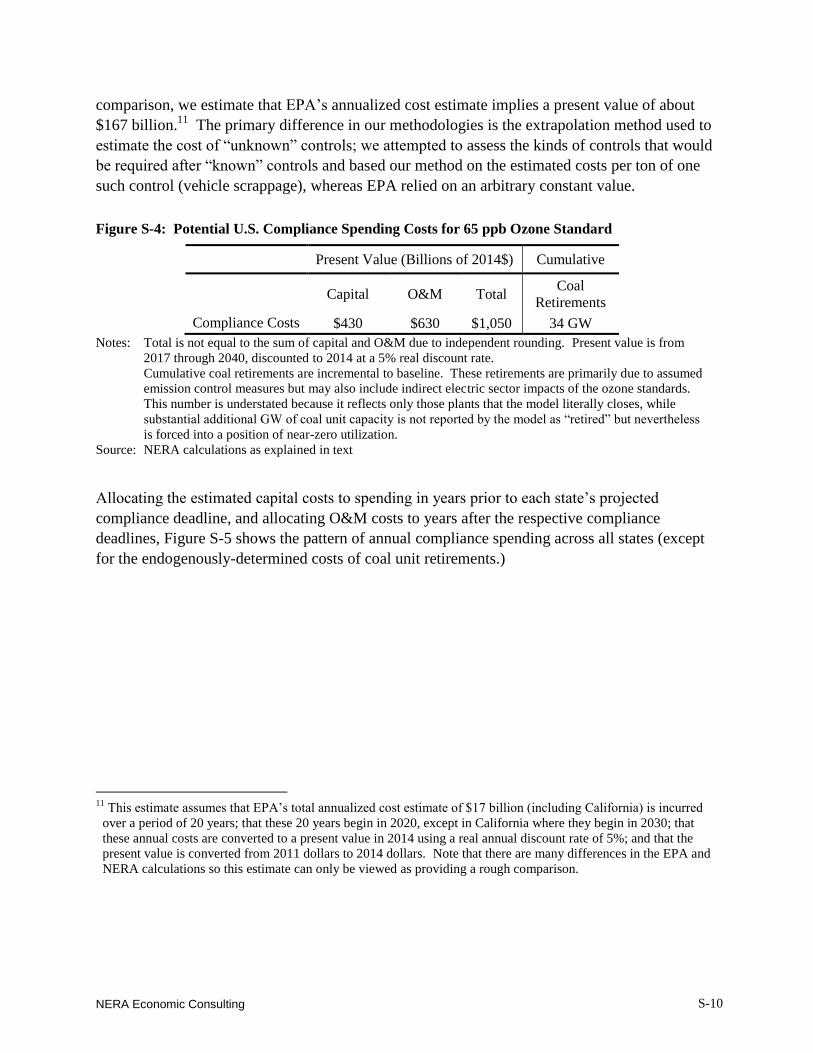
pPro

NERA Economic Consulting

S-10

comparison, we estimate that EPA’s annualized cost estimate implies a present value of about

$167 billion.11

The primary difference in our methodologies is the extrapolation method used to

estimate the cost of “unknown” controls; we attempted to assess the kinds of controls that would

be required after “known” controls and based our method on the estimated costs per ton of one

such control (vehicle scrappage), whereas EPA relied on an arbitrary constant value.

Allocating the estimated capital costs to spending in years prior to each state’s projected

compliance deadline, and allocating O&M costs to years after the respective compliance

deadlines, Figure S-5 shows the pattern of annual compliance spending across all states (except

for the endogenously-determined costs of coal unit retirements.)

11

This estimate assumes that EPA’s total annualized cost estimate of $17 billion (including California) is incurred

over a period of 20 years; that these 20 years begin in 2020, except in California where they begin in 2030; that

these annual costs are converted to a present value in 2014 using a real annual discount rate of 5%; and that the

present value is converted from 2011 dollars to 2014 dollars. Note that there are many differences in the EPA and

NERA calculations so this estimate can only be viewed as providing a rough comparison.

Figure S-4: Potential U.S. Compliance Spending Costs for 65 ppb Ozone Standard

Present Value (Billions of 2014$) Cumulative

Capital O&M Total Coal

Retirements

Compliance Costs $430 $630 $1,050 34 GW

Notes: Total is not equal to the sum of capital and O&M due to independent rounding. Present value is from

2017 through 2040, discounted to 2014 at a 5% real discount rate.

Cumulative coal retirements are incremental to baseline. These retirements are primarily due to assumed

emission control measures but may also include indirect electric sector impacts of the ozone standards.

This number is understated because it reflects only those plants that the model literally closes, while

substantial additional GW of coal unit capacity is not reported by the model as “retired” but nevertheless

is forced into a position of near-zero utilization.

Source: NERA calculations as explained in text

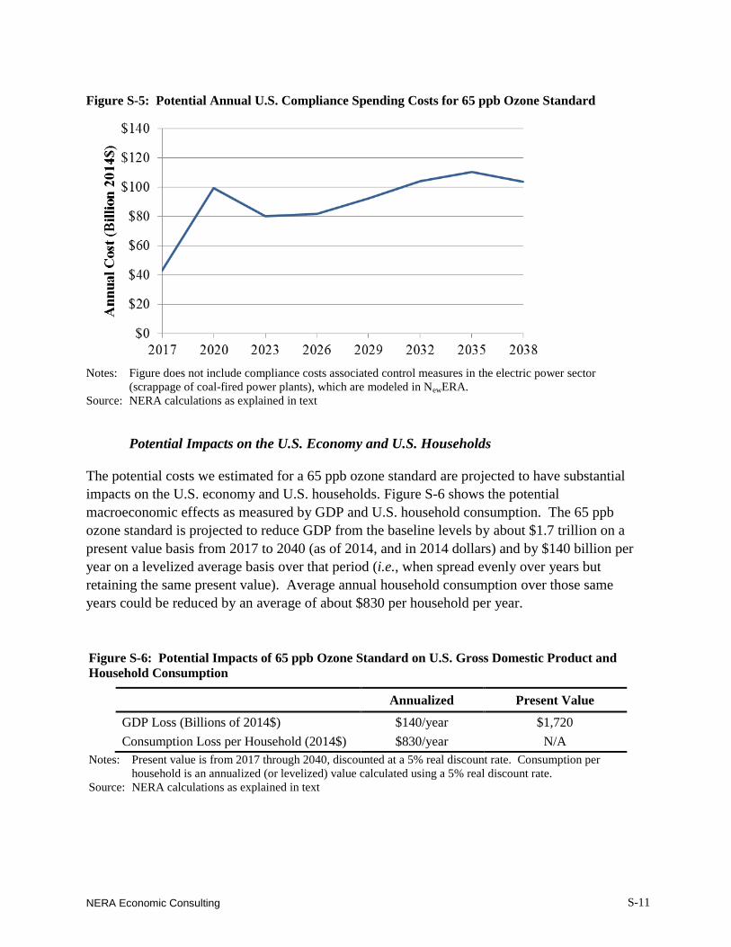
pPro

NERA Economic Consulting

S-11

Potential Impacts on the U.S. Economy and U.S. Households

The potential costs we estimated for a 65 ppb ozone standard are projected to have substantial

impacts on the U.S. economy and U.S. households. Figure S-6 shows the potential

macroeconomic effects as measured by GDP and U.S. household consumption. The 65 ppb

ozone standard is projected to reduce GDP from the baseline levels by about $1.7 trillion on a

present value basis from 2017 to 2040 (as of 2014, and in 2014 dollars) and by $140 billion per

year on a levelized average basis over that period (i.e., when spread evenly over years but

retaining the same present value). Average annual household consumption over those same

years could be reduced by an average of about $830 per household per year.

Figure S-5: Potential Annual U.S. Compliance Spending Costs for 65 ppb Ozone Standard

Notes: Figure does not include compliance costs associated control measures in the electric power sector

(scrappage of coal-fired power plants), which are modeled in NewERA.

Source: NERA calculations as explained in text

Figure S-6: Potential Impacts of 65 ppb Ozone Standard on U.S. Gross Domestic Product and

Household Consumption

Annualized Present Value

GDP Loss (Billions of 2014$) $140/year $1,720

Consumption Loss per Household (2014$) $830/year N/A

Notes: Present value is from 2017 through 2040, discounted at a 5% real discount rate. Consumption per

household is an annualized (or levelized) value calculated using a 5% real discount rate.

Source: NERA calculations as explained in text

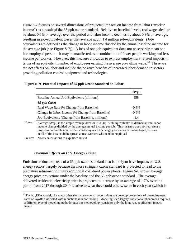
pPro

NERA Economic Consulting

S-12

Figure S-7 focuses on several dimensions of projected impacts on income from labor (“worker

income”) as a result of the 65 ppb ozone standard. Relative to baseline levels, real wages decline

by about 0.6% on average over the period and labor income declines by about 0.9% on average,

resulting in job-equivalent losses that average about 1.4 million job-equivalents. (Job-

equivalents are defined as the change in labor income divided by the annual baseline income for

the average job (see Figure S-7)). A loss of one job-equivalent does not necessarily mean one

less employed person—it may be manifested as a combination of fewer people working and less

income per worker. However, this measure allows us to express employment-related impacts in

terms of an equivalent number of employees earning the average prevailing wage.12

These are

the net effects on labor and include the positive benefits of increased labor demand in sectors

providing pollution control equipment and technologies.

Potential Effects on U.S. Energy Prices

Emissions reduction costs of a 65 ppb ozone standard also is likely to have impacts on U.S.

energy sectors, largely because the more stringent ozone standard is projected to lead to the

premature retirement of many additional coal-fired power plants. Figure S-8 shows average

energy price projections under the baseline and the 65 ppb ozone standard. The average

delivered residential electricity price is projected to increase by an average of 1.7% over the

period from 2017 through 2040 relative to what they could otherwise be in each year (which is

12

The NewERA model, like many other similar economic models, does not develop projections of unemployment

rates or layoffs associated with reductions in labor income. Modeling such largely transitional phenomena requires

a different type of modeling methodology; our methodology considers only the long-run, equilibrium impact

levels.

Figure S-7: Potential Impacts of 65 ppb Ozone Standard on Labor

Avg.

Baseline Annual Job-Equivalents (millions) 156

65 ppb Case:

Real Wage Rate (% Change from Baseline) -0.6%

Change in Labor Income (% Change from Baseline) -0.9%

Job-Equivalents (Change from Baseline, millions) -1.4

Notes: Average (Avg.) is the simple average over 2017-2040. “Job-equivalents” is defined as total labor

income change divided by the average annual income per job. This measure does not represent a

projection of numbers of workers that may need to change jobs and/or be unemployed, as some

or all of the loss could be spread across workers who remain employed

Source: NERA calculations as explained in text

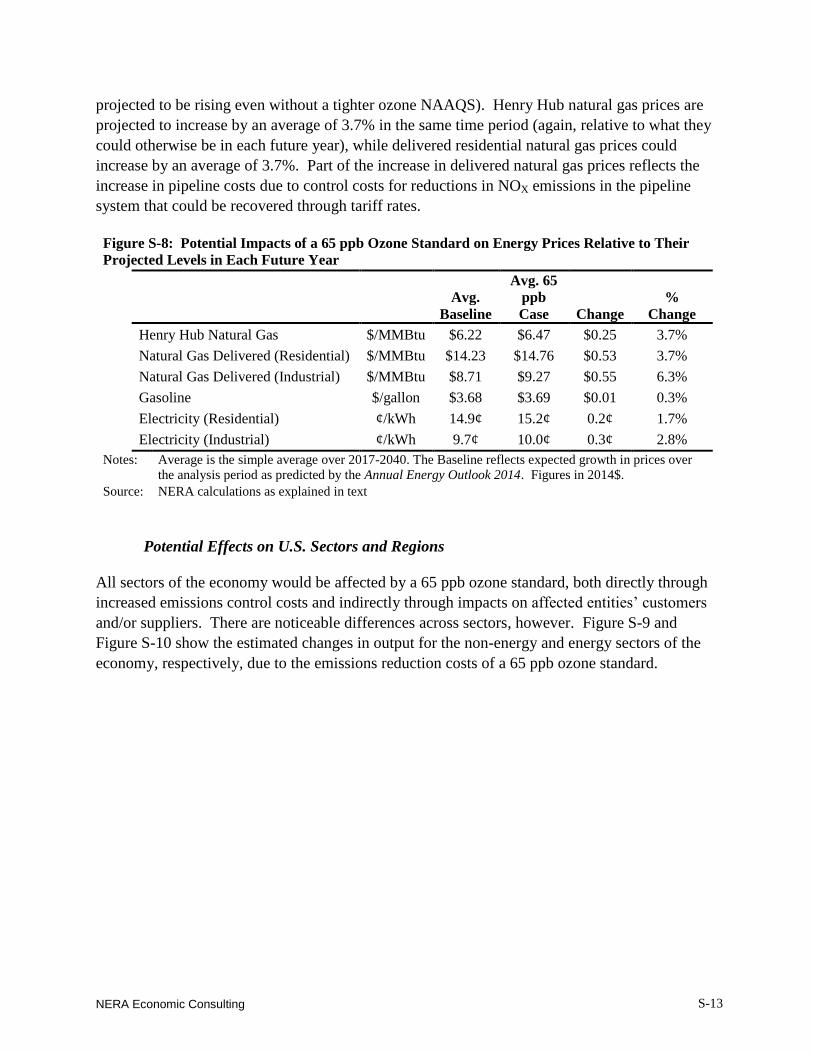
pPro

NERA Economic Consulting

S-13

projected to be rising even without a tighter ozone NAAQS). Henry Hub natural gas prices are

projected to increase by an average of 3.7% in the same time period (again, relative to what they

could otherwise be in each future year), while delivered residential natural gas prices could

increase by an average of 3.7%. Part of the increase in delivered natural gas prices reflects the

increase in pipeline costs due to control costs for reductions in NOX emissions in the pipeline

system that could be recovered through tariff rates.

Potential Effects on U.S. Sectors and Regions

All sectors of the economy would be affected by a 65 ppb ozone standard, both directly through

increased emissions control costs and indirectly through impacts on affected entities’ customers

and/or suppliers. There are noticeable differences across sectors, however. Figure S-9 and

Figure S-10 show the estimated changes in output for the non-energy and energy sectors of the

economy, respectively, due to the emissions reduction costs of a 65 ppb ozone standard.

Figure S-8: Potential Impacts of a 65 ppb Ozone Standard on Energy Prices Relative to Their

Projected Levels in Each Future Year

Avg.

Baseline

Avg. 65

ppb

Case Change

%

Change

Henry Hub Natural Gas $/MMBtu $6.22 $6.47 $0.25 3.7%

Natural Gas Delivered (Residential) $/MMBtu $14.23 $14.76 $0.53 3.7%

Natural Gas Delivered (Industrial) $/MMBtu $8.71 $9.27 $0.55 6.3%

Gasoline $/gallon $3.68 $3.69 $0.01 0.3%

Electricity (Residential) ¢/kWh 14.9¢ 15.2¢ 0.2¢ 1.7%

Electricity (Industrial) ¢/kWh 9.7¢ 10.0¢ 0.3¢ 2.8%

Notes: Average is the simple average over 2017-2040. The Baseline reflects expected growth in prices over

the analysis period as predicted by the Annual Energy Outlook 2014. Figures in 2014$.

Source: NERA calculations as explained in text

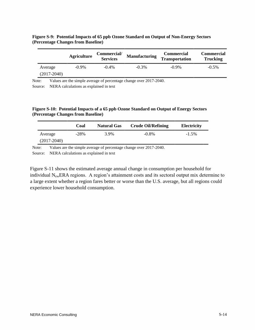
pPro

NERA Economic Consulting

S-14

Figure S-11 shows the estimated average annual change in consumption per household for

individual NewERA regions. A region’s attainment costs and its sectoral output mix determine to

a large extent whether a region fares better or worse than the U.S. average, but all regions could

experience lower household consumption.

Figure S-9: Potential Impacts of 65 ppb Ozone Standard on Output of Non-Energy Sectors

(Percentage Changes from Baseline)

Agriculture

Commercial/

Services Manufacturing

Commercial

Transportation

Commercial

Trucking

Average -0.9% -0.4% -0.3% -0.9% -0.5%

(2017-2040)

Note: Values are the simple average of percentage change over 2017-2040. Source: NERA calculations as explained in text

Figure S-10: Potential Impacts of a 65 ppb Ozone Standard on Output of Energy Sectors

(Percentage Changes from Baseline)

Coal Natural Gas Crude Oil/Refining Electricity

Average -28% 3.9% -0.8% -1.5%

(2017-2040)

Note: Values are the simple average of percentage change over 2017-2040. Source: NERA calculations as explained in text

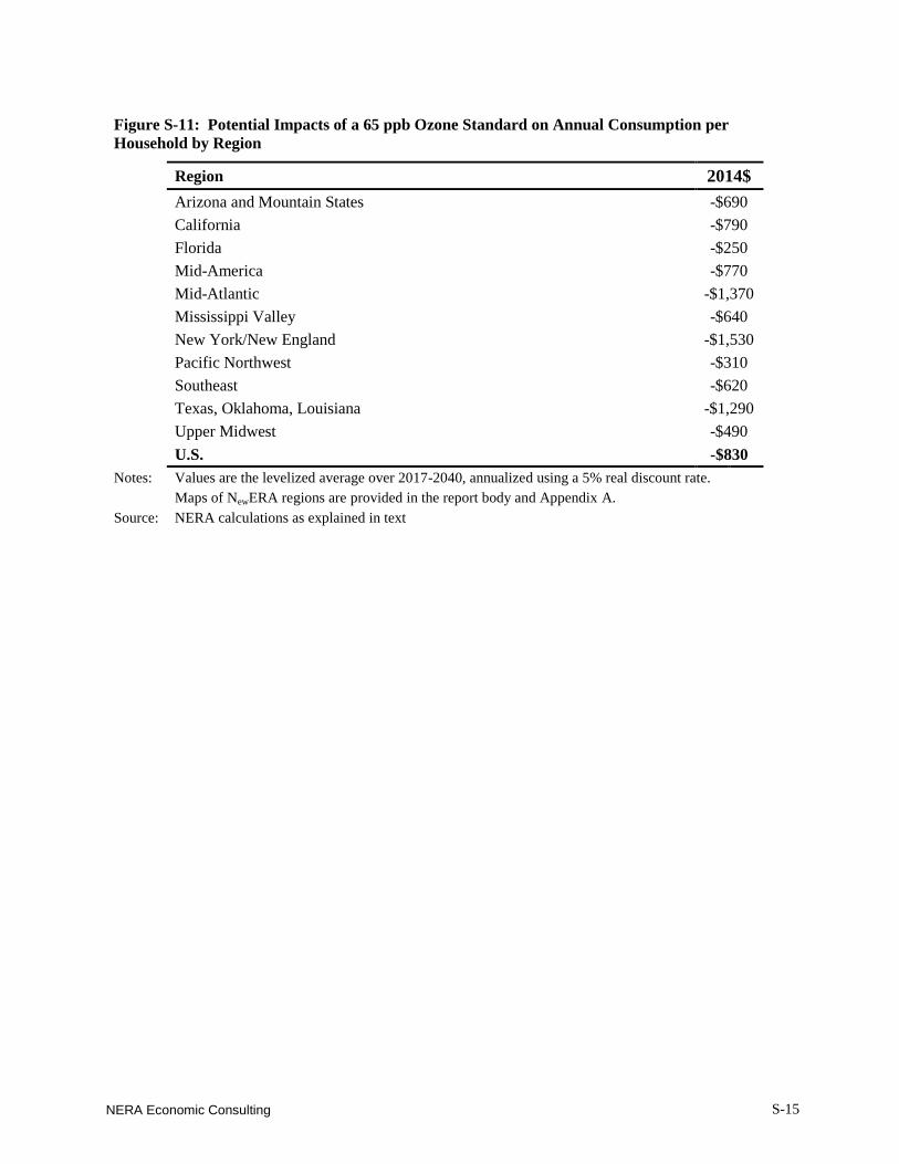
pPro

NERA Economic Consulting

S-15

Figure S-11: Potential Impacts of a 65 ppb Ozone Standard on Annual Consumption per

Household by Region

Region 2014$

Arizona and Mountain States -$690

California -$790

Florida -$250

Mid-America -$770

Mid-Atlantic -$1,370

Mississippi Valley -$640

New York/New England -$1,530

Pacific Northwest -$310

Southeast -$620

Texas, Oklahoma, Louisiana -$1,290

Upper Midwest -$490

U.S. -$830

Notes: Values are the levelized average over 2017-2040, annualized using a 5% real discount rate. Maps of NewERA regions are provided in the report body and Appendix A.

Source: NERA calculations as explained in text

pPro

NERA Economic Consulting

REFERENCES

NERA Economic Consulting (NERA). 2014. “Assessing Economic Impacts of a Stricter

National Ambient Air Quality Standard for Ozone.” July.

http://www.nera.com/publications/archive/2014/assessing-economic-impacts-of-a-

stricter-national-ambient-air-qu.html

U.S. Energy Information Administration (EIA). 2014. Annual Energy Outlook 2014.

U.S Environmental Protection Agency (EPA). 2014a. Regulatory Impact Analysis (RIA) of the

Proposed Revisions to the National Ambient Air Quality Standards (NAAQS) for Ground-

Level Ozone. http://www.epa.gov/ttnecas1/regdata/RIAs/20141125ria.pdf

U.S Environmental Protection Agency (EPA). 2014b. 2011 and 2025 NOX Emissions County

Sector Comparison.

ftp://ftp.epa.gov/EmisInventory/2011v6/ozone_naaqs/reports/2011ef_2025ef_county_sec

tor_comparison_NOX.xlsx

U.S Environmental Protection Agency (EPA). 2014c. 2011 and 2025 VOC Emissions County

Sector Comparison.

ftp://ftp.epa.gov/EmisInventory/2011v6/ozone_naaqs/reports/2011ef_2025ef_county_sec

tor_comparison_VOC.xlsx

U.S Environmental Protection Agency (EPA). 2014d. 2011, 2018, and 2025 Emissions State

Sector Comparison.

ftp://ftp.epa.gov/EmisInventory/2011v6/ozone_naaqs/reports/2011ef_2018ef_2025ef_stat

e_sector_comparison.xlsx

U.S Environmental Protection Agency (EPA). 2014e. Proposed Clean Power Plan: IPM State-

Level Emissions, Base Case. http://www.regulations.gov/#!documentDetail;D=EPA-HQ-

OAR-2013-0602-0224

U.S Environmental Protection Agency (EPA). 2014f. Proposed Clean Power Plan: IPM State-

Level Emissions, Option 1 State. http://www.regulations.gov/#!documentDetail;D=EPA-

HQ-OAR-2013-0602-0228

U.S Environmental Protection Agency (EPA). 2014g. O3 NAAQS RIA Control Strategy Results

NOX Controls for 65ppb Analysis Incremental to Baseline.

http://www.regulations.gov/#!documentDetail;D=EPA-HQ-OAR-2013-0169-0015

200 Clarendon Street

11th Floor

Boston, MA 02116

617-927-4500

1255 23rd St, NW

Suite 600

Washington, D.C. 20037

202-466-3510

www.nera.com

ATTACHMENT C

EPA Regulatory Impact Analysis of Proposed

Federal Ozone Standard: Potential Concerns

Related to EPA Compliance Cost Estimates

Prepared for:

National Association of Manufacturers

March 2015

NERA Economic Consulting

Authors

David Harrison, Jr., Ph.D.

Anne E. Smith, Ph.D.

Scott J. Bloomberg

Conor Coughlin

Christopher D’Angelo

Julia Greenberger

Carl McPherson

Andrew Stuntz

NERA Economic Consulting

200 Clarendon St, 11th Floor Boston, Massachusetts 02116

Tel: +1 617 927 4500

Fax: +1 617 927 4501

1255 23rd St, NW, Suite 600

Washington, D.C. 20037 Tel: +1 202 466 3510

Fax: +1 202 466 3605

www.nera.com

NERA Economic Consulting

Report Qualifications/Assumptions and Limiting Conditions

Information furnished by others, upon which all or portions of this report are based, is believed

to be reliable, but has not been independently verified, unless otherwise expressly indicated.

Public information and industry and statistical data are from sources we deem to be reliable;

however, we make no representation as to the accuracy or completeness of such information. The

findings contained in this report may contain predictions based on current data and historical

trends. Any such predictions are subject to inherent risks and uncertainties. NERA Economic

Consulting accepts no responsibility for actual results or future events.

The opinions expressed in this report are valid only for the purpose stated herein and as of the

date of this report. No obligation is assumed to revise this report to reflect changes, events or

conditions, which occur subsequent to the date hereof. The opinions expressed in this report do

not necessarily represent the views of NERA Economic Consulting, other NERA consultants, or

NERA’s clients.

All decisions in connection with the implementation or use of advice or recommendations

contained in this report are the sole responsibility of the client. This report does not represent

investment advice nor does it provide an opinion regarding the fairness of any transaction to any

and all parties.

© NERA Economic Consulting

NERA Economic Consulting

i

Contents

EXECUTIVE SUMMARY .......................................................................................................E-1

I. INTRODUCTION..............................................................................................................1 Background ..........................................................................................................................1 A.

Objectives of This Report ....................................................................................................1 B.

Report Organization .............................................................................................................2 C.

II. Overview of EPA’S Methodology for Estimating Emission Reductions and

Compliance Costs ...............................................................................................................3 EPA Baseline Projections of Ozone and Precursor Emissions ............................................3 A.

EPA Estimates of Required Precursor Emission Reductions and Known Controls ............6 B.

EPA Estimates of Compliance Costs .................................................................................12 C.

III. Concerns with EPA’S Emission and Compliance Cost Analysis.................................16 Concerns Related to EPA’s Determination of Compliance Emission Reductions ............16 A.

Concerns Related to EPA’s Calculation of Unknown Control Costs ................................30 B.

Summary of Concerns........................................................................................................38 C.

IV. REFERENCES .................................................................................................................40

NERA Economic Consulting

ii

List of Figures

Figure E-1. Summary of Concerns with the EPA RIA Ozone Compliance Cost Estimates ....... E-2

Figure 1. EPA 2025 “Base Case” Emissions by Source Category, Excluding California (1000s of

tons)..................................................................................................................................... 4

Figure 2. Development of EPA Baseline NOX Emissions by Source Category (tons) ................... 6

Figure 3. EPA Air Quality Modeling Regions................................................................................ 8

Figure 4. Regional Base Case NOX Emissions and Amounts of Reduction Projected to Be

Needed for Compliance with a 65 ppb Ozone Standard (Including Reductions EPA Has

Assumed Will Be Part of Its Baseline) ............................................................................. 10

Figure 5. EPA Known Control Technologies for a 65 ppb Ozone Standard (Incremental to the

EPA Baseline) ................................................................................................................... 11

Figure 6. U.S. Summary of EPA NOX Control Strategy for a 65 ppb Ozone Standard ............... 12

Figure 7. EPA Annualized Known Control Costs by Source Category for a 65 ppb Ozone

Standard (millions of 2011 dollars) .................................................................................. 13

Figure 8. EPA Annualized Unknown Control Costs by Region for a 65 ppb Ozone Standard.... 13

Figure 9. EPA Annualized Unknown Control Costs Sensitivity by Region for a 65 ppb Ozone

Standard ............................................................................................................................ 14

Figure 10. EPA Annualized Control Costs by Region for a 65 ppb Ozone Standard (Excluding

California) ......................................................................................................................... 15

Figure 11. EPA Area Classifications and Likely Attainment Dates ............................................. 17

Figure 12. “Base Case” vs. 65 ppb Compliance NOX Emissions, 2018 – 2025 (States Requiring

Reductions for 65 ppb, Excluding California) .................................................................. 20

Figure 13. Percentage NOX Reduction Required by State and Counties with Nonattaining

Monitors in the 2025 Baseline (65 ppb Standard) ............................................................ 22

Figure 14. Regional NOX Reductions and Costs by Nonattainment Status for 65 ppb (Incremental

to the EPA Baseline) ......................................................................................................... 23

Figure 15. EPA “Base Case” NOX Emissions in 2018 and 2025 (Excluding California) ............ 25

Figure 16. NOX Reductions from Baseline for a 65 ppb Ozone Standard (Excluding CA) ......... 28

Figure 17. U.S. NOX Reductions and Cost per Ton for EPA 65 ppb Control Strategy, Incremental

to EPA Baseline (Excluding California) ........................................................................... 31

NERA Economic Consulting

iii

Figure 18. Marginal Cost Curve Example of EPA Average (“Fixed”) and Hybrid Approach .... 33

Figure 19. Unknown Control Costs for 65 ppb Using EPA Average (“Fixed”) and Hybrid

Approaches, Excluding California .................................................................................... 33

Figure 20. State Marginal Cost Curve Illustrations of EPA’s 65 ppb Analysis ........................... 34

Figure 21. NOX Emissions Remaining After Known Controls for 65 ppb by Source Category by

2025 (Excluding California) ............................................................................................. 36

NERA Economic Consulting

E-1

EXECUTIVE SUMMARY

This report reviews the data and methodology the U.S. Environmental Protection Agency (EPA)

used to develop estimates of the compliance costs of a more stringent national ambient air

quality standard (NAAQS) for ozone. Our assessment is supported by numerical examples based

on emission reductions and costs of a tightening of the ozone standard to 65 parts per billion

(ppb), relative to the current standard of 75 ppb; however, the data and methodological issues we

discuss would apply to any of the alternative standards in the EPA ozone NAAQS Proposed

Rule. In its Regulatory Impact Analysis (RIA),1 EPA estimated that the additional annualized

costs of achieving a 65 ppb standard beyond costs of attaining the current standard of 75 ppb, for

areas other than California, would be about $15.4 billion per year, of which about $4.2 billion

would be “known” controls and about $11.3 billion would be “unknown” controls2 —very

substantial costs by any criterion. However, as summarized below and explained in more detail

in our report, we find that EPA’s estimate understates likely compliance costs.

Figure E-1 summarizes our assessments of the most substantial concerns we identified with

EPA’s emission reductions and cost information, divided into those affecting emission

reductions and those affecting the estimated cost per ton for emission reductions.

1 U.S. EPA, Regulatory Impact Analysis of the Proposed Revisions to the National Ambient Air Quality Standards

for Ground-Level Ozone, EPA-452/P-14-006, Office of Air and Radiation, Research Triangle Park, NC, November

2014. Available: http://www.epa.gov/ttnecas1/regdata/RIAs/20141125ria.pdf. 2 We exclude California costs in our assessments because EPA used a different methodology and presented costs for

California separately. The EPA RIA listed $1.6 billion in unknown control costs in California.

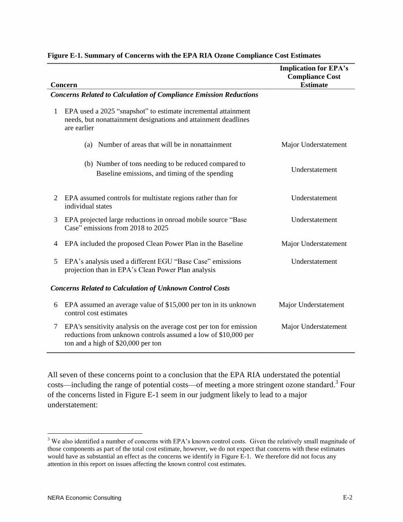
NERA Economic Consulting

E-2

All seven of these concerns point to a conclusion that the EPA RIA understated the potential

costs—including the range of potential costs—of meeting a more stringent ozone standard.3 Four

of the concerns listed in Figure E-1 seem in our judgment likely to lead to a major

understatement:

3 We also identified a number of concerns with EPA’s known control costs. Given the relatively small magnitude of

those components as part of the total cost estimate, however, we do not expect that concerns with these estimates

would have as substantial an effect as the concerns we identify in Figure E-1. We therefore did not focus any

attention in this report on issues affecting the known control cost estimates.

Figure E-1. Summary of Concerns with the EPA RIA Ozone Compliance Cost Estimates

Concern

Implication for EPA’s

Compliance Cost

Estimate

Concerns Related to Calculation of Compliance Emission Reductions

1 EPA used a 2025 “snapshot” to estimate incremental attainment

needs, but nonattainment designations and attainment deadlines

are earlier

(a) Number of areas that will be in nonattainment

(b) Number of tons needing to be reduced compared to

Baseline emissions, and timing of the spending

Major Understatement

Understatement

2 EPA assumed controls for multistate regions rather than for

individual states

Understatement

3 EPA projected large reductions in onroad mobile source “Base

Case” emissions from 2018 to 2025

Understatement

4 EPA included the proposed Clean Power Plan in the Baseline Major Understatement

5 EPA’s analysis used a different EGU “Base Case” emissions

projection than in EPA’s Clean Power Plan analysis

Understatement

Concerns Related to Calculation of Unknown Control Costs

6 EPA assumed an average value of $15,000 per ton in its unknown

control cost estimates

Major Understatement

7 EPA's sensitivity analysis on the average cost per ton for emission

reductions from unknown controls assumed a low of $10,000 per

ton and a high of $20,000 per ton

Major Understatement

NERA Economic Consulting

E-3

1. EPA used a 2025 “snapshot” to estimate incremental attainment needs, but

nonattainment designations and attainment deadlines are earlier. This assumption

understates the number of areas that will be in nonattainment as well as the number of

tons needed to be reduced compared to Baseline emissions and timing of the spending.

Areas designated as marginal or moderate would likely have attainment dates around the

end of 2020 and 2023, respectively, and would incur costs before 2025—costs that are

disregarded (by assumption) in EPA’s analysis. (Our assessment does not consider the

complications of potential reclassifications of individual non-attainment areas.)

4. EPA included the proposed Clean Power Plan (CPP) in the Baseline. EPA’s inclusion of

CPP emission reductions is not only inconsistent with its standard practice of only

including promulgated regulations, but such a deviation from standard procedure is

particularly unjustified given the enormous uncertainty in what carbon limits may

actually be applied and how states would comply, and hence what NOX emission

reductions might actually occur as a result of EPA regulation of carbon emissions from

existing electricity generating units. Without the proposed CPP in the Baseline, at least an

additional 300,000 tons of NOX reductions would be required for the 65 ppb standard,

leading to a substantial increase in the estimated compliance costs.

6. EPA assumed a constant value of $15,000 per ton for all unknown emission reductions.

Controls that EPA refers to as unknown (i.e., for which no compliance controls are

identified) represent about 40% of EPA’s estimated tons and about 73% of EPA’s

estimated costs to attain a 65 ppb ozone standard (excluding California). As one

indication of the importance of this single assumption, we calculated that unknown

control costs would have increased by about $3.7 billion per year (i.e., from $11.3 billion

to $15.0 billion, excluding California) if EPA had used an alternative methodology

presented in its own most recent prior ozone NAAQS cost assessment in 2010, as

described in the body of this report. Changing just this one aspect of the EPA

methodology would lead to a total cost estimate of $19.2 billion to achieve a 65 ppb

ozone standard (excluding California).

7. EPA assumed an uncertainty band for unknown costs of $10,000 to $20,000 per ton. This

arbitrary range seems likely to understate substantially the potential compliance costs.

Given that unknown controls would have to reduce emissions from many diffuse area or

mobile sources—since point sources are already highly controlled—the cost per ton

could be substantial (e.g., requiring early turnover of still productive capital stock such as

motor vehicles and residential or commercial heating equipment).

The other three concerns listed in Figure E-1 also suggest that the EPA RIA understated the

compliance costs of meeting a more stringent ozone standard.

2. EPA allowed for multistate controls rather than for state-by-state compliance plans.

Although the Clean Air Act requires states to develop plans to achieve the ozone

NERA Economic Consulting

E-4

standard—absent specific multi-state agreements that seem unlikely to be put in place by

the time that states would be required to submit their State Implementation Plans

(SIPs)—EPA’s modeling approach allows controls in other states to “count” toward a

state’s compliance. Since EPA’s control strategy first implemented relatively inexpensive

known controls throughout a region before moving to more expensive unknown controls,

requiring state-by-state compliance would lead to greater dependence on unknown

controls in some states and thus greater compliance costs.

3. EPA projected large reductions from 2018 to 2025 in onroad mobile sources in the

Baseline. We have identified several concerns that these Baseline reductions may be

overstated, which would have the effect of understating the emissions that need to be

reduced and thus the overall cost of a more stringent ozone standard. One corollary of

EPA’s disregard of the need for some states to achieve compliance before 2025 is that the

large reductions in mobile source emissions after actual compliance dates (the end of

2020 and 2023) would not “count” toward compliance, and hence there will be costs for

either speeding up the pace of those reductions, or making up for their absence by

attainment deadlines. An additional concern is related to the lack of documentation by

EPA of its assumptions regarding fleet turnover; fleet turnover is important because more

stringent emission standards apply to new vehicles and the actual emission reductions

thus depend in part upon the extent to which older vehicles are replaced by the lower-

emitting new vehicles. Also, the tighter CAFE standard will be reviewed in 2018 and

could be reduced if found to be too costly (as discussed in the report). If CAFE standards

were to be relaxed, the rate of NOX reductions from onroad vehicles could be less than

EPA has assumed in the Baseline. For all of these reasons, we are concerned that the

Baseline NOX reductions achievable by 2025 from this source category may be

overstated, with little likelihood that they are understated.

5. EPA used different EGU emissions in the Baseline for its ozone analysis than in the

Clean Power Plan analysis. EPA’s analysis of the CPP indicates fewer EGU NOX

emissions in the Baseline than assumed in the ozone RIA. Although we could not

determine the reasons for this difference between two recent analyses, a lower Baseline

EGU NOX level would likely imply fewer NOX reductions from the CPP than EPA

assumes in the ozone RIA, leading to an increase in the compliance costs to achieve a

more stringent ozone standard.

In summary, our evaluation suggests that EPA has understated the potential compliance costs—

including their likely range—of meeting a more stringent ozone standard. Achieving a more

stringent ozone standard could be substantially more costly than even the very substantial costs

EPA has estimated.

NERA Economic Consulting

1

I. INTRODUCTION

This report provides an assessment of the compliance cost estimates provided in the Regulatory

Impact Analysis (RIA) prepared by the U.S. Environmental Protection Agency (EPA) for its

proposed revision to the federal national ambient air quality standard (NAAQS) for ozone. We

focus on the EPA estimates of the incremental emission reductions and costs that would be

required to achieve compliance with a potential 65 parts per billion (ppb) ozone standard. As in

the RIA, all of these estimated reductions and costs are incremental to the effort needed to attain

the existing standard of 75 ppb.

Background A.

EPA Ozone Proposal 1.

EPA released its ozone proposal on November 26, 2014 and published the proposal in the

Federal Register on December 17, 2014. The current ozone standard is 75 ppb, established by

EPA in 2008. In its proposal, EPA proposed a range for revised primary and secondary ozone

standards of 65 to 70 ppb. The Agency also indicated it would take comment on a 60 ppb

standard and that it also would take comment on the option to retain the current standard.

EPA Regulatory Impact Analysis 2.

EPA released its RIA on November 26, 2014.4 The RIA provides EPA’s estimates of the

potential societal benefits and costs for the proposed ozone standards. Costs and benefits were

estimated relative to first achieving full attainment of the current standard of 75 ppb.

Objectives of This Report B.

The objectives of this report are to summarize the emission and cost information developed by

EPA in its RIA and to identify potential concerns with its accuracy. In particular, we concentrate

on EPA’s estimates of reductions in ozone precursor emissions (nitrogen oxides, or NOX, and

volatile organic compounds, or VOCs) necessary to achieve a revised ozone standard and on

EPA’s estimates of the compliance costs that would be incurred.

As noted, we limit our examples to the 65 ppb proposed standard. The issues we raise would be

relevant to other potential ozone standards, although the numerical magnitude would vary.

4 USEPA, Regulatory Impact Analysis of the Proposed Revisions to the National Ambient Air Quality Standards for

Ground-Level Ozone, EPA-452/P-14-006, Office of Air and Radiation, Research Triangle Park, NC, November

2014. Available: http://www.epa.gov/ttnecas1/regdata/RIAs/20141125ria.pdf.

NERA Economic Consulting

2

Report Organization C.

The remainder of this report is divided into two sections. Section II provides an overview of

EPA’s methodology and results. As noted, we focus on EPA’s estimates of emission reductions

and compliance costs related to a 65 ppb standard. Section III discusses concerns with the EPA’s

estimates, prioritizing the concerns as “major” concerns and “additional” concerns.

NERA Economic Consulting

3

II. OVERVIEW OF EPA’S METHODOLOGY FOR ESTIMATING

EMISSION REDUCTIONS AND COMPLIANCE COSTS

This section provides an overview of EPA’s methodology for estimating the potential emission

reductions and compliance costs to achieve a proposed ozone standard of 65 ppb, relative to the

current standard of 75 ppb. We summarize EPA’s analysis in terms of three basic steps:

1. Develop a Baseline projection of ozone levels and precursor emissions;

2. Estimate the state-level reductions in emissions from the Baseline needed to comply

with alternative ozone standards and identify “known” and “unknown” controls to

achieve those reductions; and

3. Estimate the costs of the emission controls needed to comply with alternative ozone

standards.

The sections below summarize EPA’s methodology and results for each of these three steps. We

do not include EPA’s estimates for California, which are based on a different methodology than

that developed for the other states. Note that in some cases we provide comments on EPA’s

methodology that indicate our concerns with EPA’s methodology; these concerns are developed

in more detail in Section III of this report.

EPA Baseline Projections of Ozone and Precursor Emissions A.

The costs of attaining a new ozone standard depend on ambient air quality in the future,

consistent with the timing of the attainment deadlines that areas will face under a revised ozone

standard. EPA developed a Baseline projection of ozone concentrations and precursor emissions

for the year 2025. The 2025 information formed the basis for a 2025 “snapshot” analysis of

annualized attainment costs.

The EPA Baseline was developed by modifying a 2025 “Base Case” projection to reflect three

additional modifications: (1) EPA’s proposed Clean Power Plan (CPP), (2) the current ozone

NAAQS (75 ppb), and (3) post-2025 vehicle emissions in California.

The 2025 “Base Case” Emissions Projection 1.

EPA began its analysis with the Ozone NAAQS Emissions Modeling Platform (2011v6.1),

which projected NOX, VOC, and other emissions from 2011 inventory levels to future years

2018 and 2025. This projection included most regulations and programs currently “on the

books,” including MATS, CAIR, most NSPS, and Tier 3 vehicle standards.

Emissions in this EPA “Base Case” projection are divided into sectors of emissions sources,

which we group into five emissions “source categories”:

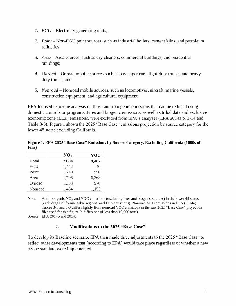
NERA Economic Consulting

4

1. EGU – Electricity generating units;

2. Point – Non-EGU point sources, such as industrial boilers, cement kilns, and petroleum

refineries;

3. Area – Area sources, such as dry cleaners, commercial buildings, and residential

buildings;

4. Onroad – Onroad mobile sources such as passenger cars, light-duty trucks, and heavy-

duty trucks; and

5. Nonroad – Nonroad mobile sources, such as locomotives, aircraft, marine vessels,

construction equipment, and agricultural equipment.

EPA focused its ozone analysis on those anthropogenic emissions that can be reduced using

domestic controls or programs. Fires and biogenic emissions, as well as tribal data and exclusive

economic zone (EEZ) emissions, were excluded from EPA’s analyses (EPA 2014a p. 3-14 and

Table 3-3). Figure 1 shows the 2025 “Base Case” emissions projection by source category for the

lower 48 states excluding California.

Modifications to the 2025 “Base Case” 2.

To develop its Baseline scenario, EPA then made three adjustments to the 2025 “Base Case” to

reflect other developments that (according to EPA) would take place regardless of whether a new

ozone standard were implemented.

Figure 1. EPA 2025 “Base Case” Emissions by Source Category, Excluding California (1000s of

tons)

NOX VOC

Total 7,684 9,487

EGU 1,442 40

Point 1,749 950

Area 1,706 6,368

Onroad 1,333 976

Nonroad 1,454 1,153

Note: Anthropogenic NOX and VOC emissions (excluding fires and biogenic sources) in the lower 48 states

(excluding California, tribal regions, and EEZ emissions). Nonroad VOC emissions in EPA (2014a)

Tables 3-1 and 3-3 differ slightly from nonroad VOC emissions in the raw 2025 “Base Case” projection

files used for this figure (a difference of less than 10,000 tons).

Source: EPA 2014b and 2014c

NERA Economic Consulting

5

a. EPA’s Proposed Clean Power Plan

EPA adjusted the 2025 “Base Case” emissions to reflect compliance with EPA’s proposed CPP

under section 111(d) of the Clean Air Act. The impact of the CPP on NOX emissions was

estimated using simulations conducted with the IPM model of Option 1 of the CPP Proposed

Rule,5 and assuming “state-level compliance” with that option (EPA 2014a p. 4-1, 4-5, and 3-

11).6

b. The Current Ozone NAAQS (75 ppb)

EPA further adjusted 2025 “Base Case” emissions to reflect compliance with the current ozone

NAAQS of 75 ppb. EPA projected that 11 counties, all in California or Texas, would exceed the

current 75 ppb standard in 2025 in the Base Case (EPA 2014a, Figure 4-1). Emission controls

and compliance costs associated with meeting the current standard are not attributable to a new

ozone NAAQS, so EPA includes them in the EPA Baseline.

c. Post-2025 Vehicle Emissions in California

EPA notes that parts of California probably would not be required to meet a new ozone standard

until sometime in the 2030s (EPA 2014a p. 1-9). When simulating costs to attain the new

standard in California, EPA attempted to look at incremental tons that would need to be reduced

in the 2030s, rather than in 2025. Thus, for California’s attainment costs, EPA developed a

Baseline from the 2025 inventory that is intended to reflect a yet-later year, called “post-2025.”

This “post-2025” Baseline for California includes an additional reduction of 14,000 tons of NOX

and 6,000 tons of VOC that EPA projected will occur between 2025 and 2030 due to further

implementation of current vehicle regulations (EPA 2014a, p. 1-9, 3A-25).

Due to the later attainment year in California, EPA presented California information separately

from the rest of the lower 48 states in its RIA. For consistency with the non-California tables in

the EPA RIA, we have excluded California from all tables and figures in this report.

5 EPA estimated that Option 1 in the CPP Proposed Rule would reduce U.S. CO2 power plant emissions by 30% in

2030, relative to the 2005 emission level. (Option 2 would have less stringent emission rate targets and different

compliance timing.) This analysis was based on emission rate targets developed using four “Building Blocks” –

heat rate improvements at coal units, increased utilization of natural gas combined cycle units, increases in

renewables and nuclear energy, and increases in end-use energy efficiency.

6 We presume that EPA adjusted only NOX emissions to get from its Ozone NAAQS “Base Case” to the Ozone

NAAQS Baseline. This presumption is based on our review of EPA’s statements about VOCs in the RIA for the

CPP Proposed Rule; this document suggests that EPA may have estimated VOC emissions changes due to the CPP

in calculations outside of its compliance modeling (EPA 2014h, p. 4A-7), but it later states that VOC emissions

changes from the CPP are insignificant as a reason why EPA did not account for them when assessing ozone co-

benefits of the CPP Proposed Rule (EPA 2014h, 4A-17). Even if EPA did include undocumented VOC reductions

from the CPP Proposed Rule in constructing the ozone NAAQS Baseline, this adjustment would have had minimal

effect on emissions and cost estimates.

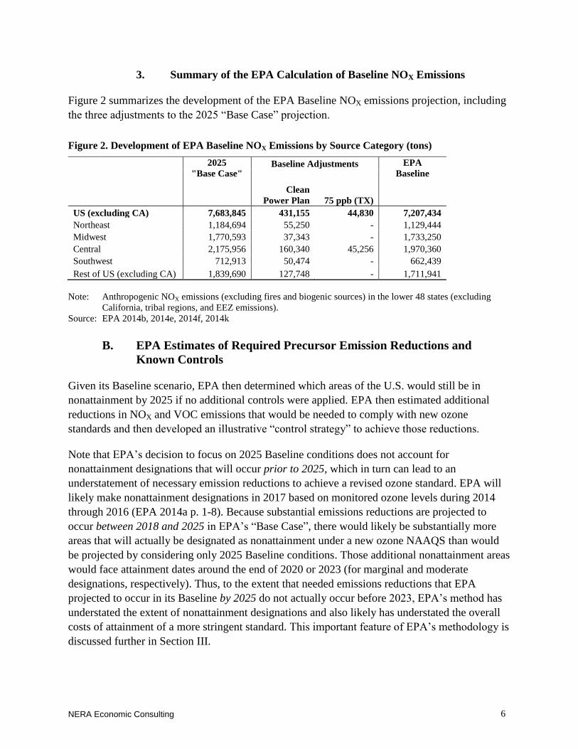
NERA Economic Consulting

6

Summary of the EPA Calculation of Baseline NOX Emissions 3.

Figure 2 summarizes the development of the EPA Baseline NOX emissions projection, including

the three adjustments to the 2025 “Base Case” projection.

EPA Estimates of Required Precursor Emission Reductions and B.

Known Controls

Given its Baseline scenario, EPA then determined which areas of the U.S. would still be in

nonattainment by 2025 if no additional controls were applied. EPA then estimated additional

reductions in NOX and VOC emissions that would be needed to comply with new ozone

standards and then developed an illustrative “control strategy” to achieve those reductions.

Note that EPA’s decision to focus on 2025 Baseline conditions does not account for

nonattainment designations that will occur prior to 2025, which in turn can lead to an

understatement of necessary emission reductions to achieve a revised ozone standard. EPA will

likely make nonattainment designations in 2017 based on monitored ozone levels during 2014

through 2016 (EPA 2014a p. 1-8). Because substantial emissions reductions are projected to

occur between 2018 and 2025 in EPA’s “Base Case”, there would likely be substantially more

areas that will actually be designated as nonattainment under a new ozone NAAQS than would

be projected by considering only 2025 Baseline conditions. Those additional nonattainment areas

would face attainment dates around the end of 2020 or 2023 (for marginal and moderate

designations, respectively). Thus, to the extent that needed emissions reductions that EPA

projected to occur in its Baseline by 2025 do not actually occur before 2023, EPA’s method has

understated the extent of nonattainment designations and also likely has understated the overall

costs of attainment of a more stringent standard. This important feature of EPA’s methodology is

discussed further in Section III.

Figure 2. Development of EPA Baseline NOX Emissions by Source Category (tons)

2025

"Base Case" Baseline Adjustments EPA

Baseline

Clean

Power Plan 75 ppb (TX)

US (excluding CA) 7,683,845 431,155 44,830 7,207,434

Northeast 1,184,694 55,250 - 1,129,444

Midwest 1,770,593 37,343 - 1,733,250

Central 2,175,956 160,340 45,256 1,970,360

Southwest 712,913 50,474 - 662,439

Rest of US (excluding CA) 1,839,690 127,748 - 1,711,941

Note: Anthropogenic NOX emissions (excluding fires and biogenic sources) in the lower 48 states (excluding

California, tribal regions, and EEZ emissions).

Source: EPA 2014b, 2014e, 2014f, 2014k

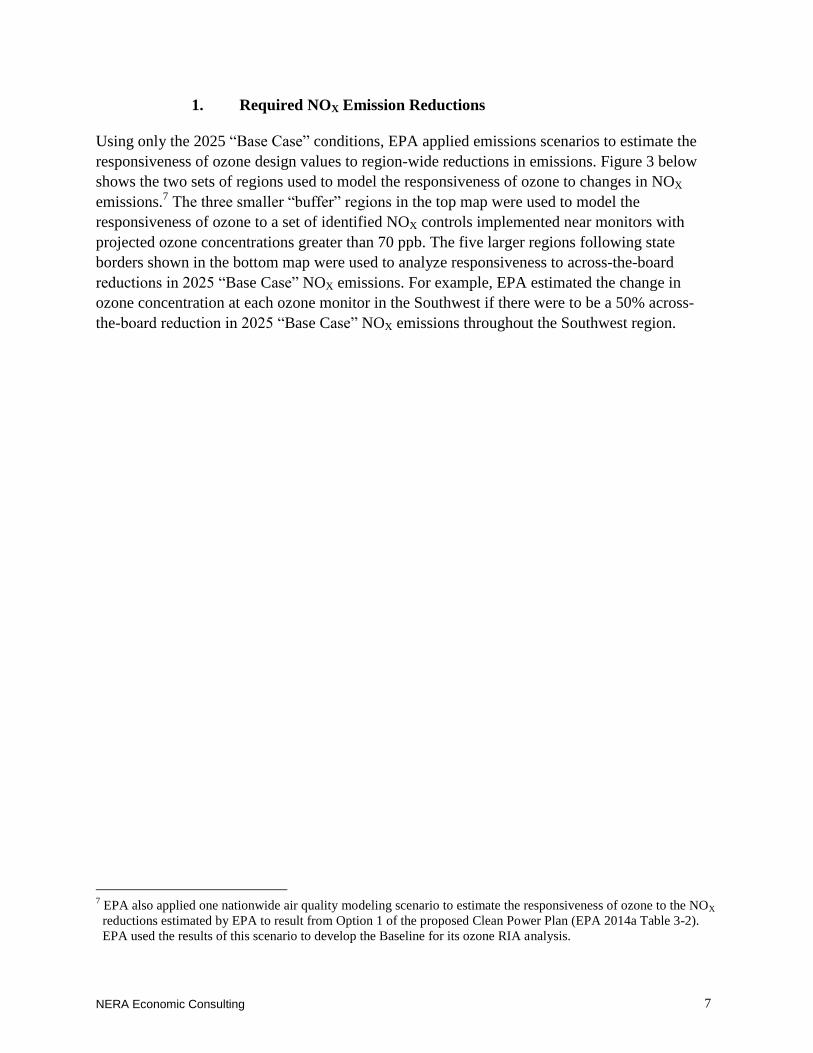
NERA Economic Consulting

7

Required NOX Emission Reductions 1.

Using only the 2025 “Base Case” conditions, EPA applied emissions scenarios to estimate the

responsiveness of ozone design values to region-wide reductions in emissions. Figure 3 below

shows the two sets of regions used to model the responsiveness of ozone to changes in NOX

emissions.7 The three smaller “buffer” regions in the top map were used to model the

responsiveness of ozone to a set of identified NOX controls implemented near monitors with

projected ozone concentrations greater than 70 ppb. The five larger regions following state

borders shown in the bottom map were used to analyze responsiveness to across-the-board

reductions in 2025 “Base Case” NOX emissions. For example, EPA estimated the change in

ozone concentration at each ozone monitor in the Southwest if there were to be a 50% across-

the-board reduction in 2025 “Base Case” NOX emissions throughout the Southwest region.

7 EPA also applied one nationwide air quality modeling scenario to estimate the responsiveness of ozone to the NOX

reductions estimated by EPA to result from Option 1 of the proposed Clean Power Plan (EPA 2014a Table 3-2).

EPA used the results of this scenario to develop the Baseline for its ozone RIA analysis.

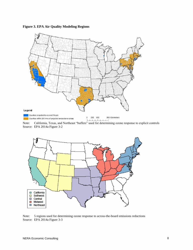
NERA Economic Consulting

8

Figure 3. EPA Air Quality Modeling Regions

Note: California, Texas, and Northeast “buffers” used for determining ozone response to explicit controls

Source: EPA 2014a Figure 3-2

Note: 5 regions used for determining ozone response to across-the-board emissions reductions

Source: EPA 2014a Figure 3-3

NERA Economic Consulting

9

These air quality scenarios resulted in estimates of “relative response factors” – the approximate

change in ozone design values at an ozone monitor estimated to result from a regional change in

precursor emissions. To determine how many tons of emission reductions would be required to

meet each alternative ozone standard, EPA applied emission reductions within each of the

regions until the ozone concentration at every monitor within the respective region (as calculated

using the “relative response factors”) was projected to meet that standard.8 Figure 4 shows each

region’s 2025 “Base Case” NOX emissions (as the full length of each horizontal bar), the

regional emission reductions EPA assumed would be part of the RIA’s Baseline (i.e., the grey

portions of each bar), and additional NOX reductions EPA projected to be needed to comply with

a 65 ppb standard in EPA’s analysis (green portions of each bar). The remainder of each bar (the

blue portion) shows the total tons of NOX that EPA estimates may remain in each region while

fully attaining the 65 ppb alternative standard. That remainder is called “compliance emissions.”

As noted above, these results are based on EPA’s approach that determined incremental tons of

reduction needed for attainment only when the year 2025 has been reached, whereas the

nonattainment designations will be based on conditions that exist prior to 2018, and EPA expects

most of the associated attainment deadlines to be around the end of 2020 or 2023 (EPA 2014a p.

1-8).

8 Note that EPA excluded 26 rural or remote monitors in the West and Southwest from its analysis due to low

modeled responsiveness to NOX reductions, mostly due to transport from California and Mexico (EPA 2014a p.

3A-54). EPA suggests that these areas could pursue regulatory relief from a tighter ozone NAAQS. EPA projected

that all 26 of these excluded monitors would be in attainment with a 70 ppb ozone standard in EPA’s 2025

Baseline, but 15 of these monitors are projected to exceed a 65 ppb ozone standard. To the extent that these areas

are unable to obtain exemptions from NAAQS requirements, they could require additional emissions reductions

(and control costs) that are not captured in EPA’s analysis.

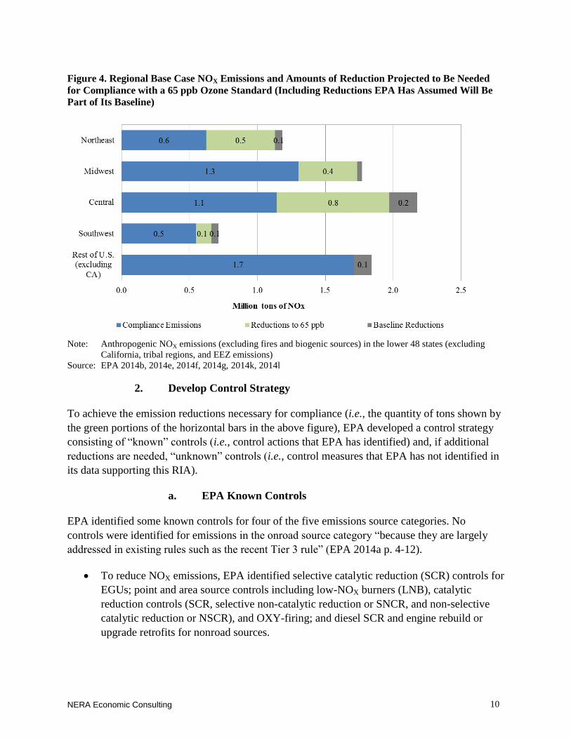
NERA Economic Consulting

10

Develop Control Strategy 2.

To achieve the emission reductions necessary for compliance (i.e., the quantity of tons shown by

the green portions of the horizontal bars in the above figure), EPA developed a control strategy

consisting of “known” controls (i.e., control actions that EPA has identified) and, if additional

reductions are needed, “unknown” controls (i.e., control measures that EPA has not identified in

its data supporting this RIA).

a. EPA Known Controls

EPA identified some known controls for four of the five emissions source categories. No

controls were identified for emissions in the onroad source category “because they are largely

addressed in existing rules such as the recent Tier 3 rule” (EPA 2014a p. 4-12).

To reduce NOX emissions, EPA identified selective catalytic reduction (SCR) controls for

EGUs; point and area source controls including low-NOX burners (LNB), catalytic

reduction controls (SCR, selective non-catalytic reduction or SNCR, and non-selective

catalytic reduction or NSCR), and OXY-firing; and diesel SCR and engine rebuild or

upgrade retrofits for nonroad sources.

Figure 4. Regional Base Case NOX Emissions and Amounts of Reduction Projected to Be Needed

for Compliance with a 65 ppb Ozone Standard (Including Reductions EPA Has Assumed Will Be

Part of Its Baseline)

Note: Anthropogenic NOX emissions (excluding fires and biogenic sources) in the lower 48 states (excluding

California, tribal regions, and EEZ emissions)

Source: EPA 2014b, 2014e, 2014f, 2014g, 2014k, 2014l

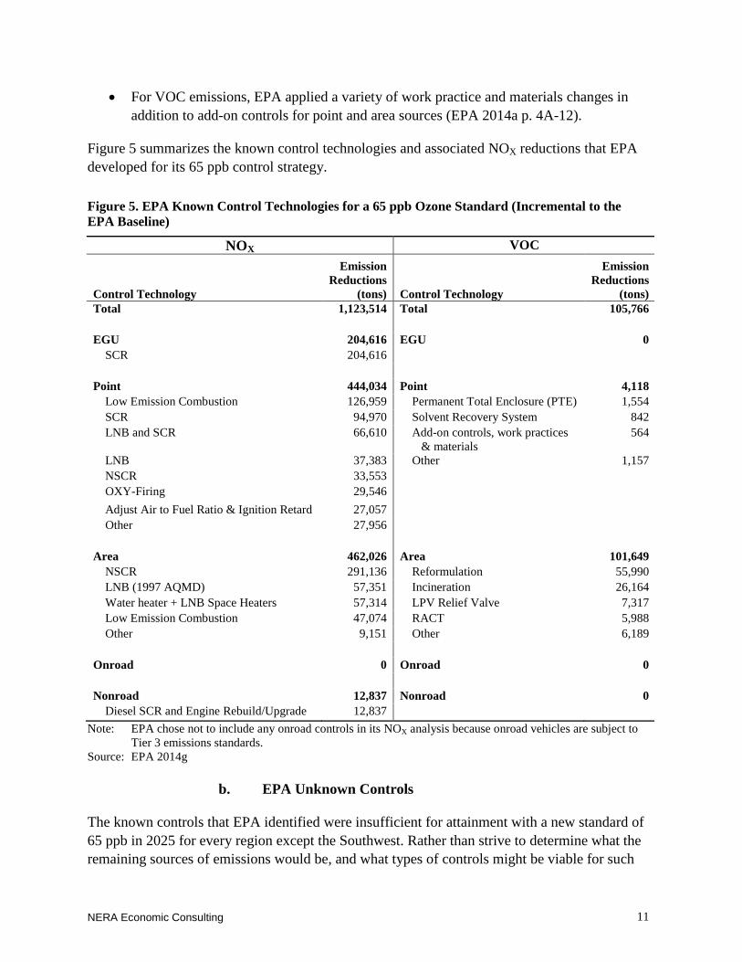
NERA Economic Consulting

11

For VOC emissions, EPA applied a variety of work practice and materials changes in

addition to add-on controls for point and area sources (EPA 2014a p. 4A-12).

Figure 5 summarizes the known control technologies and associated NOX reductions that EPA

developed for its 65 ppb control strategy.

b. EPA Unknown Controls

The known controls that EPA identified were insufficient for attainment with a new standard of

65 ppb in 2025 for every region except the Southwest. Rather than strive to determine what the

remaining sources of emissions would be, and what types of controls might be viable for such

Figure 5. EPA Known Control Technologies for a 65 ppb Ozone Standard (Incremental to the

EPA Baseline)

NOX VOC

Control Technology

Emission

Reductions

(tons) Control Technology

Emission

Reductions

(tons)

Total 1,123,514 Total 105,766

EGU 204,616 EGU 0

SCR 204,616

Point 444,034 Point 4,118

Low Emission Combustion 126,959 Permanent Total Enclosure (PTE) 1,554

SCR 94,970 Solvent Recovery System 842

LNB and SCR 66,610 Add-on controls, work practices

& materials

564

LNB 37,383 Other 1,157

NSCR 33,553

OXY-Firing 29,546

Adjust Air to Fuel Ratio & Ignition Retard 27,057

Other 27,956

Area 462,026 Area 101,649

NSCR 291,136 Reformulation 55,990

LNB (1997 AQMD) 57,351 Incineration 26,164

Water heater + LNB Space Heaters 57,314 LPV Relief Valve 7,317

Low Emission Combustion 47,074 RACT 5,988

Other 9,151 Other 6,189

Onroad 0 Onroad 0

Nonroad 12,837 Nonroad 0

Diesel SCR and Engine Rebuild/Upgrade 12,837

Note: EPA chose not to include any onroad controls in its NOX analysis because onroad vehicles are subject to

Tier 3 emissions standards.

Source: EPA 2014g

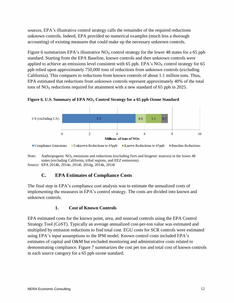
NERA Economic Consulting

12

sources, EPA’s illustrative control strategy calls the remainder of the required reductions

unknown controls. Indeed, EPA provided no numerical examples (much less a thorough

accounting) of existing measures that could make up the necessary unknown controls.

Figure 6 summarizes EPA’s illustrative NOX control strategy for the lower 48 states for a 65 ppb

standard. Starting from the EPA Baseline, known controls and then unknown controls were

applied to achieve an emissions level consistent with 65 ppb. EPA’s NOX control strategy for 65

ppb relied upon approximately 750,000 tons of reductions from unknown controls (excluding

California). This compares to reductions from known controls of about 1.1 million tons. Thus,

EPA estimated that reductions from unknown controls represent approximately 40% of the total

tons of NOX reductions required for attainment with a new standard of 65 ppb in 2025.

EPA Estimates of Compliance Costs C.

The final step in EPA’s compliance cost analysis was to estimate the annualized costs of

implementing the measures in EPA’s control strategy. The costs are divided into known and

unknown controls.

Cost of Known Controls 1.

EPA estimated costs for the known point, area, and nonroad controls using the EPA Control

Strategy Tool (CoST). Typically an average annualized cost-per-ton value was estimated and

multiplied by emission reductions to find total cost. EGU costs for SCR controls were estimated

using EPA’s input assumptions to the IPM model. Known control costs included EPA’s

estimates of capital and O&M but excluded monitoring and administrative costs related to

demonstrating compliance. Figure 7 summarizes the cost per ton and total cost of known controls

in each source category for a 65 ppb ozone standard.

Figure 6. U.S. Summary of EPA NOX Control Strategy for a 65 ppb Ozone Standard

Note: Anthropogenic NOX emissions and reductions (excluding fires and biogenic sources) in the lower 48

states (excluding California, tribal regions, and EEZ emissions)

Source: EPA 2014b, 2014e, 2014f, 2014g, 2014k, 2014l

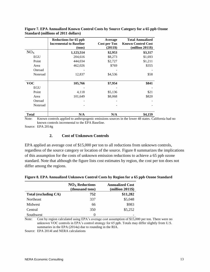
NERA Economic Consulting

13

Cost of Unknown Controls 2.

EPA applied an average cost of $15,000 per ton to all reductions from unknown controls,

regardless of the source category or location of the source. Figure 8 summarizes the implications

of this assumption for the costs of unknown emission reductions to achieve a 65 ppb ozone

standard. Note that although the figure lists cost estimates by region, the cost per ton does not

differ among the regions.

Figure 7. EPA Annualized Known Control Costs by Source Category for a 65 ppb Ozone

Standard (millions of 2011 dollars)

Reductions for 65 ppb

Incremental to Baseline

(tons)

Average

Cost per Ton

(2011$)

Total Annualized

Known Control Cost

(million 2011$)

NOX 1,123,514 $2,953 $3,317

EGU 204,616 $8,273 $1,693

Point 444,034 $2,727 $1,211

Area 462,026 $769 $355

Onroad - - -

Nonroad 12,837 $4,536 $58

VOC 105,766 $7,954 $841

EGU - - -

Point 4,118 $5,136 $21

Area 101,649 $8,068 $820

Onroad - - -

Nonroad - - -

Total N/A N/A $4,159

Note: Known controls applied to anthropogenic emissions sources in the lower 48 states. California had no

known controls incremental to the EPA Baseline.

Source: EPA 2014g

Figure 8. EPA Annualized Unknown Control Costs by Region for a 65 ppb Ozone Standard

NOX Reductions

(thousand tons)

Annualized Cost

(million 2011$)

Total (excluding CA) 752 $11,282

Northeast 337 $5,048

Midwest 66 $983

Central 350 $5,252

Southwest 0 - Note: Cost by region calculated using EPA’s average cost assumption of $15,000 per ton. There were no

unknown VOC controls in EPA’s control strategy for 65 ppb. Totals may differ slightly from U.S.

summaries in the EPA (2014a) due to rounding in the RIA.

Source: EPA 2014l and NERA calculations

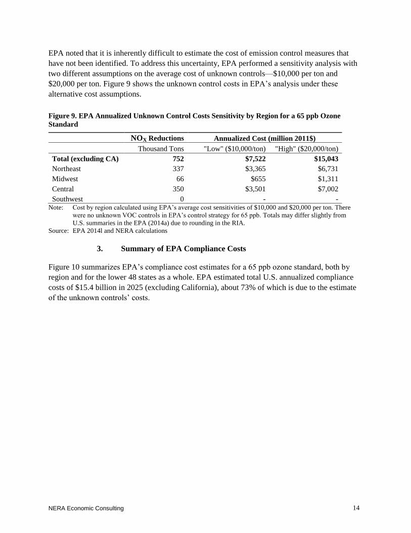
NERA Economic Consulting

14

EPA noted that it is inherently difficult to estimate the cost of emission control measures that

have not been identified. To address this uncertainty, EPA performed a sensitivity analysis with

two different assumptions on the average cost of unknown controls—$10,000 per ton and

$20,000 per ton. Figure 9 shows the unknown control costs in EPA’s analysis under these

alternative cost assumptions.

Summary of EPA Compliance Costs 3.

Figure 10 summarizes EPA’s compliance cost estimates for a 65 ppb ozone standard, both by

region and for the lower 48 states as a whole. EPA estimated total U.S. annualized compliance

costs of $15.4 billion in 2025 (excluding California), about 73% of which is due to the estimate

of the unknown controls’ costs.

Figure 9. EPA Annualized Unknown Control Costs Sensitivity by Region for a 65 ppb Ozone

Standard

NOX Reductions Annualized Cost (million 2011$)

Thousand Tons "Low" ($10,000/ton) "High" ($20,000/ton)

Total (excluding CA) 752 $7,522 $15,043

Northeast 337 $3,365 $6,731

Midwest 66 $655 $1,311

Central 350 $3,501 $7,002

Southwest 0 - - Note: Cost by region calculated using EPA’s average cost sensitivities of $10,000 and $20,000 per ton. There

were no unknown VOC controls in EPA’s control strategy for 65 ppb. Totals may differ slightly from

U.S. summaries in the EPA (2014a) due to rounding in the RIA.

Source: EPA 2014l and NERA calculations

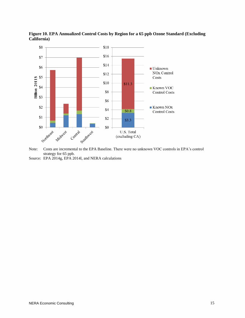
NERA Economic Consulting

15

Figure 10. EPA Annualized Control Costs by Region for a 65 ppb Ozone Standard (Excluding

California)

Note: Costs are incremental to the EPA Baseline. There were no unknown VOC controls in EPA’s control

strategy for 65 ppb.

Source: EPA 2014g, EPA 2014l, and NERA calculations

NERA Economic Consulting

16

III. CONCERNS WITH EPA’S EMISSION AND COMPLIANCE COST

ANALYSIS

This section summarizes our reviews of the emissions and cost information in the EPA RIA. We

organize the review and discussion into two major areas.

1. Concerns related to EPA’s determination of required emission reductions; and

2. Concerns related to EPA’s estimates of unknown control costs.

For each of the individual issues, we summarize the key EPA assumption and then discuss

potential concerns with the methodology and the implications of the concerns for EPA’s

estimated compliance costs. Where possible, we provide quantitative assessments of the

magnitude of potential error. The final subsection provides our summary of the potential

significance of these concerns.

Concerns Related to EPA’s Determination of Compliance Emission A.

Reductions

EPA Assumed All States Would Need to Comply in 2025 Although 1.

Some States Are Likely to Require Compliance Earlier

a. EPA Assumption Regarding Compliance Date

Under the Clean Air Act, if the ozone NAAQS is revised in 2015 as planned, nonattainment

areas will be designated and assigned classifications and attainment years based on ozone design

value data available in 2017. Design values are three-year averages of certified monitor readings,

and so the nonattainment designations will be based on monitor readings taken during 2014

through 2016. In short, nonattainment with the proposed new ozone NAAQS will be determined

based on essentially current conditions. Following the 2017 designations, states would then

develop control strategies and implement controls over a period of years such that each

nonattainment area’s design value will be at the level of the new standard by its specified

attainment year. Given current data, it is reasonable to expect that most areas that would be

designated nonattainment in 2017 with a 65 ppb potential standard would be classified as either

marginal or moderate status, with attainment dates around the end of 2020 and 2023,

respectively. Areas that fail to comply by their attainment dates would be reclassified to a higher

category, with the attendant more burdensome regulatory restrictions.

EPA’s RIA cost analysis did not reflect these legal requirements. Instead, EPA performed a

“snapshot” analysis of annualized compliance costs in 2025, citing three reasons:

1. Data and resource limitations made it difficult to estimate multiple years of costs (EPA

2014a, p. ES-14);

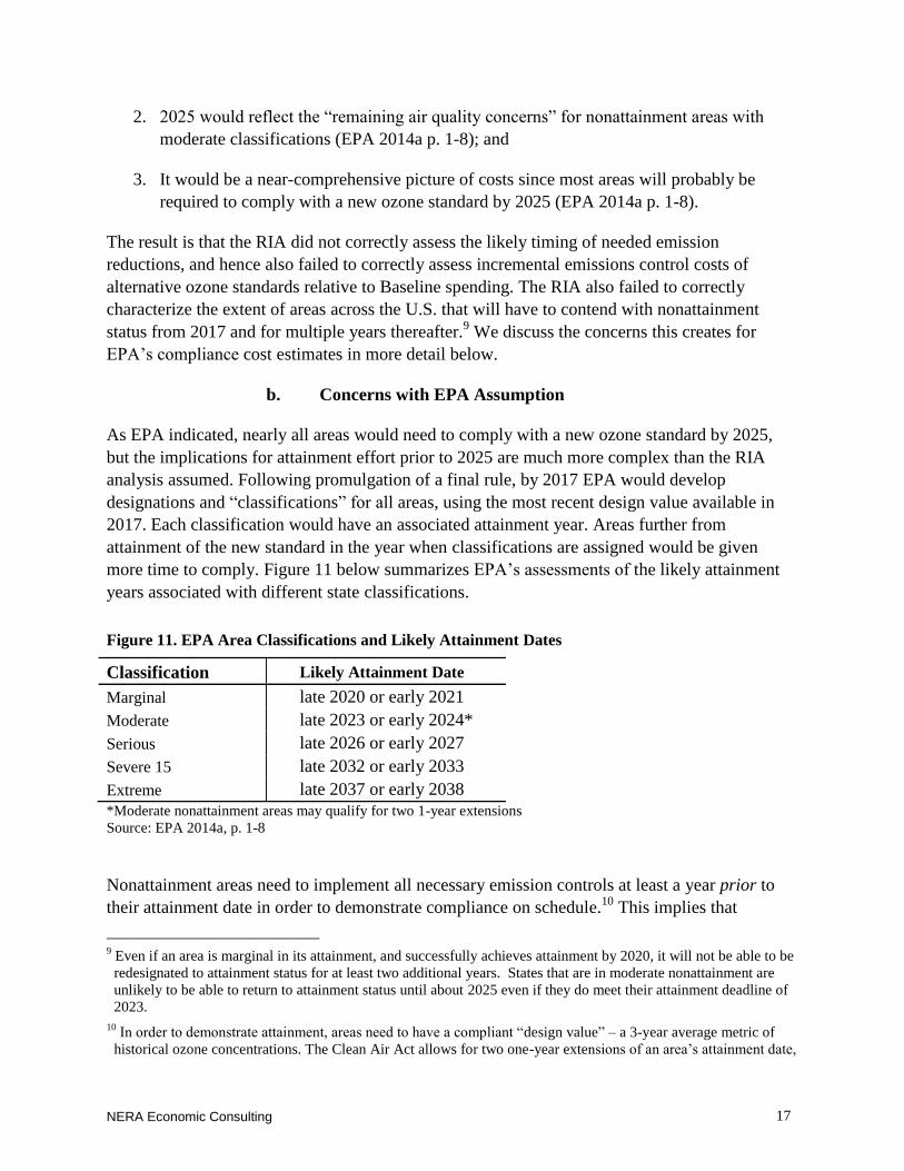
NERA Economic Consulting

17

2. 2025 would reflect the “remaining air quality concerns” for nonattainment areas with

moderate classifications (EPA 2014a p. 1-8); and

3. It would be a near-comprehensive picture of costs since most areas will probably be

required to comply with a new ozone standard by 2025 (EPA 2014a p. 1-8).

The result is that the RIA did not correctly assess the likely timing of needed emission

reductions, and hence also failed to correctly assess incremental emissions control costs of

alternative ozone standards relative to Baseline spending. The RIA also failed to correctly

characterize the extent of areas across the U.S. that will have to contend with nonattainment

status from 2017 and for multiple years thereafter.9 We discuss the concerns this creates for

EPA’s compliance cost estimates in more detail below.

b. Concerns with EPA Assumption

As EPA indicated, nearly all areas would need to comply with a new ozone standard by 2025,

but the implications for attainment effort prior to 2025 are much more complex than the RIA

analysis assumed. Following promulgation of a final rule, by 2017 EPA would develop

designations and “classifications” for all areas, using the most recent design value available in

2017. Each classification would have an associated attainment year. Areas further from

attainment of the new standard in the year when classifications are assigned would be given

more time to comply. Figure 11 below summarizes EPA’s assessments of the likely attainment

years associated with different state classifications.

Nonattainment areas need to implement all necessary emission controls at least a year prior to

their attainment date in order to demonstrate compliance on schedule.10

This implies that

9 Even if an area is marginal in its attainment, and successfully achieves attainment by 2020, it will not be able to be

redesignated to attainment status for at least two additional years. States that are in moderate nonattainment are

unlikely to be able to return to attainment status until about 2025 even if they do meet their attainment deadline of

2023.

10 In order to demonstrate attainment, areas need to have a compliant “design value” – a 3-year average metric of

historical ozone concentrations. The Clean Air Act allows for two one-year extensions of an area’s attainment date,

Figure 11. EPA Area Classifications and Likely Attainment Dates

Classification Likely Attainment Date

Marginal late 2020 or early 2021

Moderate late 2023 or early 2024*

Serious late 2026 or early 2027

Severe 15 late 2032 or early 2033

Extreme late 2037 or early 2038

*Moderate nonattainment areas may qualify for two 1-year extensions

Source: EPA 2014a, p. 1-8

NERA Economic Consulting

18

marginal areas would need to implement all controls prior to the area’s ozone season in 2020 for

an attainment date in early 2021, and moderate areas would need to implement all controls prior

to the area’s ozone season in 2023 for attainment in early 2024. (Available monitoring data

indicate that nearly all areas that are likely to be designated as nonattainment would probably fall

into the marginal or moderate classification for any of the proposed alternative standards.)

Despite these facts, in the RIA EPA implicitly equates the need for potential reductions to

achieve attainment in 2025 (based on 2025 emission levels) with an area’s attainment

designation, which would be based on emission levels prior to area designations in 2017 or 2018.

EPA’s 2025 analysis does not indicate the number of areas of the U.S. that can be expected to

fall into nonattainment in 2017 as a result of a downward revision of the ozone standard in 2015,

but rather focuses on areas that will still have design values above the NAAQS in 2025. In

reality, additional areas outside of the regions EPA projects will need more emissions reductions

as of 2025 might be designated as nonattainment based on recent historical ozone concentrations

and may need to come into attainment prior to 2025. The effect of EPA’s approach is not only to

understate the extent of nonattainment designations that will be made in 2017, but also to

understate the timing of emissions reduction needs, and the potential number of reductions

relative to the earlier Baseline years. EPA’s cost analysis does not account for the need for some

portion of its 2025 Baseline emissions reductions to occur at least two years earlier than EPA has

projected them to occur – and at least five years earlier if marginally-classified areas are to avoid

being bumped up to the more onerous moderate classification after 2020.

As a result, using 2025 for a “snapshot” analysis of emissions, reduction needs, and costs

initially appears complete, but is misleadingly so because it is in effect assuming that marginal

and moderate states will be able to take advantage of Baseline emissions reductions that EPA

projects will not occur until after their required (pre-2025) attainment dates. The most

significant concern is for marginal areas, which would need to implement controls by 2020;

ozone precursor emissions in these areas would need to be reduced from their Baseline level

down to a level consistent with attainment by 2020, while EPA’s analysis does not “check” for

this outcome until 2025. Baseline emissions are projected to decline over time from 2018

through 2025, so greater reductions would be needed for attainment at the end of 2020 than in

2025.

Our assessment does not take into account the additional legal and administrative complications

that might arise for some nonattainment areas. The Clean Air Act does provide some flexibility

with respect to attainment dates, but this flexibility usually comes with increased requirements

and costs. Moreover, whether the flexibility is granted and what additional requirements (and

costs) would be involved is difficult to assess. EPA did not provide such assessments as a

but one year of historical concentrations below the ozone NAAQS (with one allowed exceedance) is still required

by the attainment date (Clean Air Act, Section 181(a)(5)) in order to avoid being “bumped up” to a more severe

classification, with attending more burdensome regulatory restrictions on the designated regions’ emitters and

governments.

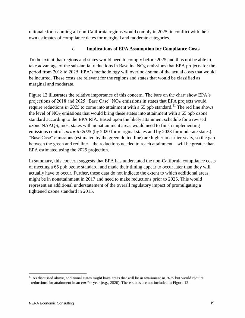
NERA Economic Consulting

19

rationale for assuming all non-California regions would comply in 2025, in conflict with their

own estimates of compliance dates for marginal and moderate categories.

c. Implications of EPA Assumption for Compliance Costs

To the extent that regions and states would need to comply before 2025 and thus not be able to

take advantage of the substantial reductions in Baseline NOX emissions that EPA projects for the

period from 2018 to 2025, EPA’s methodology will overlook some of the actual costs that would

be incurred. These costs are relevant for the regions and states that would be classified as

marginal and moderate.

Figure 12 illustrates the relative importance of this concern. The bars on the chart show EPA’s

projections of 2018 and 2025 “Base Case” NOX emissions in states that EPA projects would

require reductions in 2025 to come into attainment with a 65 ppb standard.11

The red line shows

the level of NOX emissions that would bring these states into attainment with a 65 ppb ozone

standard according to the EPA RIA. Based upon the likely attainment schedule for a revised

ozone NAAQS, most states with nonattainment areas would need to finish implementing

emissions controls prior to 2025 (by 2020 for marginal states and by 2023 for moderate states).

“Base Case” emissions (estimated by the green dotted line) are higher in earlier years, so the gap

between the green and red line—the reductions needed to reach attainment—will be greater than

EPA estimated using the 2025 projection.

In summary, this concern suggests that EPA has understated the non-California compliance costs

of meeting a 65 ppb ozone standard, and made their timing appear to occur later than they will

actually have to occur. Further, these data do not indicate the extent to which additional areas

might be in nonattainment in 2017 and need to make reductions prior to 2025. This would

represent an additional understatement of the overall regulatory impact of promulgating a

tightened ozone standard in 2015.

11

As discussed above, additional states might have areas that will be in attainment in 2025 but would require

reductions for attainment in an earlier year (e.g., 2020). These states are not included in Figure 12.

NERA Economic Consulting

20

EPA Assumes Controls for Multistate Regions Rather than for 2.

Individual States

a. EPA Assumption

As discussed in Section II, EPA estimated the emission reductions needed to comply with

alternative ozone standards using regional air quality modeling scenarios and the implied

response factors at ozone monitors (i.e., the responsiveness of ozone monitors to regional

reductions in ozone precursor emissions). In broad terms, EPA first applied known NOX and

VOC controls within each region, locating emission reductions near the monitors with the

highest ozone readings where possible but ultimately extending throughout each region (EPA

2014a p. 3-24). If known controls alone could not bring all of the ozone monitors in a region into

attainment, EPA then applied region-wide emission reductions from unknown controls.

Figure 12. “Base Case” vs. 65 ppb Compliance NOX Emissions, 2018 – 2025 (States Requiring

Reductions for 65 ppb, Excluding California)

Note: Figure includes only states that required NOX reductions as part of EPA’s control strategy for 65 ppb,

excluding California. The “compliance emissions” level consistent with an ozone concentration of 65 ppb

is derived from EPA’s 2025 “snapshot” analysis and assumed to be constant across years.

Source: EPA 2014a, 2014d, and NERA calculations as described in text

NERA Economic Consulting

21

b. Concerns with EPA Assumption

As EPA acknowledged, the illustrative control strategy in the EPA RIA has little geographic

specificity (EPA 2014a p. 3-23). Under EPA’s approach, known controls were applied in specific

locations, but they were applied in any location where they might be found within the multi-state

region, even if they were not located in a state with a nonattaining monitor, or in close proximity

to a nonattaining monitor within the state. Similarly, unknown controls were applied without any

locational specificity across the entire multi-state region until all monitors throughout that region

reached attainment. Applying reductions in such broad strokes using response factors is

necessarily crude. EPA attempted to improve its estimates by performing multiple air quality

modeling sensitivities in some regions,12

but there is still significant uncertainty in this approach

(even beyond the uncertainty inherent in any air quality modeling projection). To our knowledge,

EPA did not perform air quality modeling of its final control strategies that would serve as a

“check” that the final combination of regional controls in EPA’s analysis (which were developed

using response factors) actually corresponds closely to attainment in all areas.

Beyond general uncertainty, there are two potential issues with this modeling approach, both of

which were acknowledged in the EPA RIA. First, except in a few areas along regional borders,

EPA did not account for emissions transport across regions.13

EPA concluded that this could lead

to an overstatement of emission reductions necessary for compliance since downwind regions

might benefit from emissions reductions in upwind regions (EPA 2014a p. 3-23). However, to

the degree that regional ozone concentrations are affected by transport, the conditions in upwind

regions could also increase the need for local emissions reductions; the net effect of ignoring

regional transport on required emission reductions is ambiguous.

Second, EPA’s approach hinges on the assumption that states in the same region would choose to

coordinate their control strategies. More specifically, EPA’s analysis implicitly assumes that

states with less severe nonattainment areas or with no nonattainment areas at all would

implement control measures to help other states (either by choice or requirement). Figure 13

shows the percentage NOX reductions from the EPA Baseline in each state for a 65 ppb standard.

The figure also indicates counties where EPA projects monitors in nonattainment with a potential

65 ppb ozone standard in the 2025 Baseline.

12

These additional sensitivities captured some of the nonlinearity in the responsiveness of ozone concentrations to

NOX emissions reductions.

13 Except for monitors in Pittsburgh, Buffalo, and the Illinois suburbs of St. Louis, which fell along regional borders,

monitors were assumed to only be affected by within-region emission changes (EPA 2014a p. 3-23).

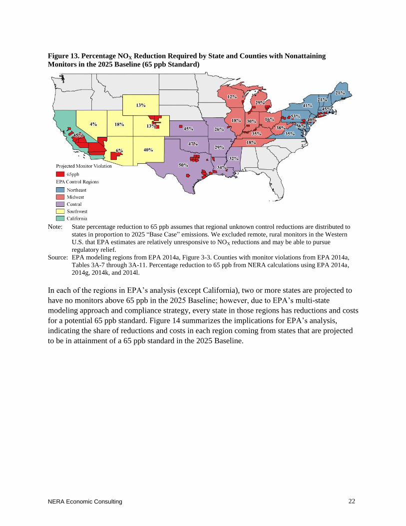
NERA Economic Consulting

22

In each of the regions in EPA’s analysis (except California), two or more states are projected to

have no monitors above 65 ppb in the 2025 Baseline; however, due to EPA’s multi-state

modeling approach and compliance strategy, every state in those regions has reductions and costs

for a potential 65 ppb standard. Figure 14 summarizes the implications for EPA’s analysis,

indicating the share of reductions and costs in each region coming from states that are projected

to be in attainment of a 65 ppb standard in the 2025 Baseline.

Figure 13. Percentage NOX Reduction Required by State and Counties with Nonattaining

Monitors in the 2025 Baseline (65 ppb Standard)

Note: State percentage reduction to 65 ppb assumes that regional unknown control reductions are distributed to

states in proportion to 2025 “Base Case” emissions. We excluded remote, rural monitors in the Western

U.S. that EPA estimates are relatively unresponsive to NOX reductions and may be able to pursue

regulatory relief.

Source: EPA modeling regions from EPA 2014a, Figure 3-3. Counties with monitor violations from EPA 2014a,

Tables 3A-7 through 3A-11. Percentage reduction to 65 ppb from NERA calculations using EPA 2014a,

2014g, 2014k, and 2014l.

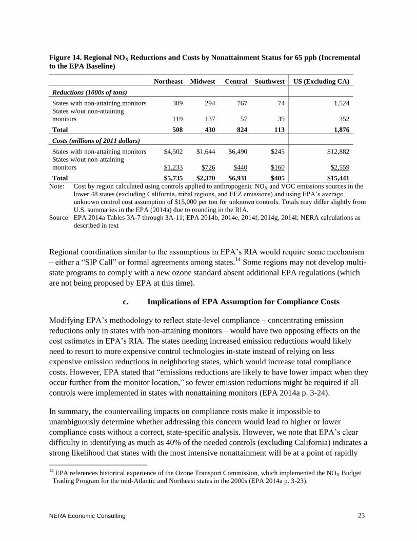
NERA Economic Consulting

23

Regional coordination similar to the assumptions in EPA’s RIA would require some mechanism

– either a “SIP Call” or formal agreements among states.14

Some regions may not develop multi-

state programs to comply with a new ozone standard absent additional EPA regulations (which

are not being proposed by EPA at this time).

c. Implications of EPA Assumption for Compliance Costs

Modifying EPA’s methodology to reflect state-level compliance – concentrating emission

reductions only in states with non-attaining monitors – would have two opposing effects on the

cost estimates in EPA’s RIA. The states needing increased emission reductions would likely

need to resort to more expensive control technologies in-state instead of relying on less

expensive emission reductions in neighboring states, which would increase total compliance

costs. However, EPA stated that “emissions reductions are likely to have lower impact when they

occur further from the monitor location,” so fewer emission reductions might be required if all

controls were implemented in states with nonattaining monitors (EPA 2014a p. 3-24).

In summary, the countervailing impacts on compliance costs make it impossible to

unambiguously determine whether addressing this concern would lead to higher or lower

compliance costs without a correct, state-specific analysis. However, we note that EPA’s clear

difficulty in identifying as much as 40% of the needed controls (excluding California) indicates a

strong likelihood that states with the most intensive nonattainment will be at a point of rapidly

14

EPA references historical experience of the Ozone Transport Commission, which implemented the NOX Budget

Trading Program for the mid-Atlantic and Northeast states in the 2000s (EPA 2014a p. 3-23).

Figure 14. Regional NOX Reductions and Costs by Nonattainment Status for 65 ppb (Incremental

to the EPA Baseline)

Northeast Midwest Central Southwest US (Excluding CA)

Reductions (1000s of tons)

States with non-attaining monitors 389 294 767 74 1,524

States w/out non-attaining

monitors 119 137 57 39 352

Total 508 430 824 113 1,876

Costs (millions of 2011 dollars)

States with non-attaining monitors $4,502 $1,644 $6,490 $245 $12,882

States w/out non-attaining

monitors $1,233 $726 $440 $160 $2,559

Total $5,735 $2,370 $6,931 $405 $15,441

Note: Cost by region calculated using controls applied to anthropogenic NOX and VOC emissions sources in the

lower 48 states (excluding California, tribal regions, and EEZ emissions) and using EPA’s average

unknown control cost assumption of $15,000 per ton for unknown controls. Totals may differ slightly from

U.S. summaries in the EPA (2014a) due to rounding in the RIA.

Source: EPA 2014a Tables 3A-7 through 3A-11; EPA 2014b, 2014e, 2014f, 2014g, 2014l; NERA calculations as

described in text

NERA Economic Consulting

24

increasing marginal costs of control. Our own analyses (discussed below) support this

possibility. Rapidly increasing marginal costs could easily dominate the need for somewhat

fewer tons of reduction if those reductions are shifted to in-state sources. In fact, some of the

assumed out-of-state emissions reductions may occur closer to the nonattainment area than

would additional in-state controls, since nonattainment areas are often near state borders (see

Figure 14).15

At a minimum, we note that the RIA’s approach of allowing controls from out of

state to be a significant part of the assumed control strategy is too far from the reality of control

strategies for its cost estimates to be considered reliable. EPA should provide an analysis that

does include state-by-state compliance strategies.16

EPA Finds Large Reductions in Mobile Source “Base Case” 3.

Emissions from 2018 to 2025

a. EPA Assumption

As discussed above, EPA’s compliance cost analysis was based on an emissions projection for

2025. EPA projects a dramatic decrease in “Base Case” onroad and nonroad NOX emissions

between 2018 and 2025. This decrease reflects both implementation of on-the-books emissions

standards for onroad vehicles (including Tier 3 standards), off-road equipment, and marine

vessels, as well as projected vehicle usage patterns and vehicle fleet turnover. EPA’s projected

“Base Case” NOX emissions in 2018 and 2025 are summarized by emissions source category in

Figure 15.

15

Additionally, ozone forms from precursors emitted at sometimes relatively long distances. In fact, precursor

emissions reductions can decrease ozone concentrations in their local vicinity, even as they elevate ozone

concentrations at more distant locations.

16 We also note, however, that doing so will be uninformative unless EPA also adopts a more realistic way to deal

with whether marginal costs are increasing as more and more unknown controls are assumed, as we discuss later in

this section.

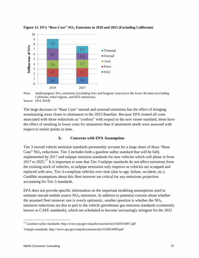
NERA Economic Consulting

25

The large decrease in “Base Case” onroad and nonroad emissions has the effect of bringing

nonattaining areas closer to attainment in the 2025 Baseline. Because EPA treated all costs

associated with those reductions as “costless” with respect to the new ozone standard, these have

the effect of resulting in lower costs for attainment than if attainment needs were assessed with

respect to earlier points in time.

b. Concerns with EPA Assumption

Tier 3 onroad vehicle emission standards presumably account for a large share of these “Base

Case” NOX reductions. Tier 3 includes both a gasoline sulfur standard that will be fully

implemented by 2017 and tailpipe emission standards for new vehicles which will phase in from

2017 to 2025.17

It is important to note that Tier 3 tailpipe standards do not affect emissions from

the existing stock of vehicles, so tailpipe emissions only improve as vehicles are scrapped and

replaced with new, Tier-3-compliant vehicles over time (due to age, failure, accident, etc.).

Credible assumptions about this fleet turnover are critical for any emissions projection

accounting for Tier 3 standards.

EPA does not provide specific information on the important modeling assumptions used to

estimate onroad mobile source NOX emissions. In addition to potential concern about whether

the assumed fleet turnover rate is overly optimistic, another question is whether the NOX

emission reductions are due in part to the vehicle greenhouse gas emission standards (commonly

known as CAFE standards), which are scheduled to become increasingly stringent for the 2022

17

Gasoline sulfur standards: http://www.epa.gov/otaq/documents/tier3/420f14007.pdf

Tailpipe standards: http://www.epa.gov/otaq/documents/tier3/420f14009.pdf

Figure 15. EPA “Base Case” NOX Emissions in 2018 and 2025 (Excluding California)

Note: Anthropogenic NOX emissions (excluding fires and biogenic sources) in the lower 48 states (excluding

California, tribal regions, and EEZ emissions).

Source: EPA 2014b

NERA Economic Consulting

26

through 2025 model years. These standards are subject to a mid-term evaluation in 2018, which

could result in less stringent requirements, and thereby result in fewer Baseline NOX reductions

(e.g., through fewer electric cars in the fleet). In all, the onroad NOX reductions by 2025 may not

be as large as EPA calculated, and if so, costs to attain the new NAAQS would be understated.

Even without these understatement concerns, the need for some of those reductions to occur

earlier than 2025 does imply an understatement of compliance costs.

c. Implications of EPA Assumption

We were unable to analyze the fleet turnover assumptions or the effect of the greenhouse gas

emission standards in EPA’s onroad mobile emissions modeling for this report, so their

implication for EPA’s compliance cost estimates based on the 2025 conditions alone (as EPA

relies on) is uncertain. If the reduction in onroad and nonroad emissions from 2018 to 2025 is

overstated, additional emission controls would be required and EPA’s compliance cost estimates

would be understated; if the onroad and nonroad reductions were understated in EPA’s 2025

“Base Case” projection, the compliance cost estimates would be overstated.

However, there is a more important concern with the reliance on the projected large downward

trend in mobile source emissions that is not as ambiguous in its direction, and it is tied to the

problematic use of the 2025 “snapshot” for determining the proposed rule’s cost. It is quite clear

that what may appear to be “anyway” attainment considered from the vantage point of 2025

could be hiding more extensive nonattainment starting substantially earlier. Much of those

Baseline mobile source reductions may need to be sped up in time to deal with the need to reduce

emissions for some regions and states substantially earlier than 2025. That will imply costs that

the EPA RIA did not account for, and at earlier dates. Thus, even if the fleet turnover

assumptions prove correct, the RIA would understate compliance costs by relying on that fleet

turnover through 2025.

Furthermore, because the mobile source reductions are not under EPA’s control, but depend on

actual consumer decisions about when to buy new vehicles, the method for obtaining those

reductions earlier than Baseline is either relatively costly incentives for early vehicle scrappage,

or finding other types of controls that can be mandated directly by the regulator, which are

presently unidentifiable (and hence also likely to have relatively higher marginal costs than

EPA’s RIA is assuming).

In summary, the heavy reliance of the RIA cost estimates on mobile source emissions reduction

that will only occur gradually and which are not directly under the control of regulators has

resulted in an understatement. We also note that given the importance of the dramatic reduction

in mobile source emissions as a general matter, a reader of EPA’s RIA should be concerned that

projected vehicle age distributions and turnover are not discussed plainly and supported by

evidence in either the EPA RIA or in the support documentation for the “Base Case” projection.

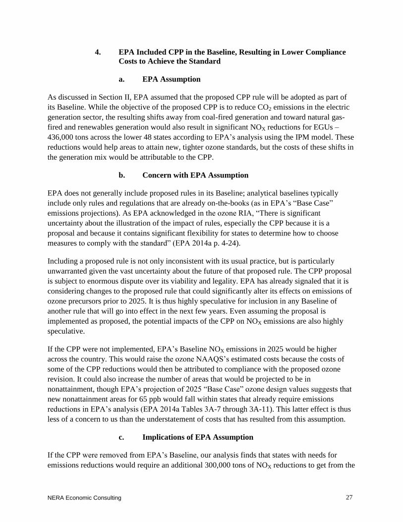
NERA Economic Consulting

27

EPA Included CPP in the Baseline, Resulting in Lower Compliance 4.

Costs to Achieve the Standard

a. EPA Assumption

As discussed in Section II, EPA assumed that the proposed CPP rule will be adopted as part of

its Baseline. While the objective of the proposed CPP is to reduce CO2 emissions in the electric

generation sector, the resulting shifts away from coal-fired generation and toward natural gas-

fired and renewables generation would also result in significant NOX reductions for EGUs –

436,000 tons across the lower 48 states according to EPA’s analysis using the IPM model. These

reductions would help areas to attain new, tighter ozone standards, but the costs of these shifts in

the generation mix would be attributable to the CPP.

b. Concern with EPA Assumption

EPA does not generally include proposed rules in its Baseline; analytical baselines typically

include only rules and regulations that are already on-the-books (as in EPA’s “Base Case”

emissions projections). As EPA acknowledged in the ozone RIA, “There is significant

uncertainty about the illustration of the impact of rules, especially the CPP because it is a

proposal and because it contains significant flexibility for states to determine how to choose

measures to comply with the standard” (EPA 2014a p. 4-24).

Including a proposed rule is not only inconsistent with its usual practice, but is particularly

unwarranted given the vast uncertainty about the future of that proposed rule. The CPP proposal

is subject to enormous dispute over its viability and legality. EPA has already signaled that it is

considering changes to the proposed rule that could significantly alter its effects on emissions of

ozone precursors prior to 2025. It is thus highly speculative for inclusion in any Baseline of

another rule that will go into effect in the next few years. Even assuming the proposal is

implemented as proposed, the potential impacts of the CPP on NOX emissions are also highly

speculative.

If the CPP were not implemented, EPA’s Baseline NOX emissions in 2025 would be higher

across the country. This would raise the ozone NAAQS’s estimated costs because the costs of

some of the CPP reductions would then be attributed to compliance with the proposed ozone

revision. It could also increase the number of areas that would be projected to be in

nonattainment, though EPA’s projection of 2025 “Base Case” ozone design values suggests that

new nonattainment areas for 65 ppb would fall within states that already require emissions

reductions in EPA’s analysis (EPA 2014a Tables 3A-7 through 3A-11). This latter effect is thus

less of a concern to us than the understatement of costs that has resulted from this assumption.

c. Implications of EPA Assumption

If the CPP were removed from EPA’s Baseline, our analysis finds that states with needs for

emissions reductions would require an additional 300,000 tons of NOX reductions to get from the

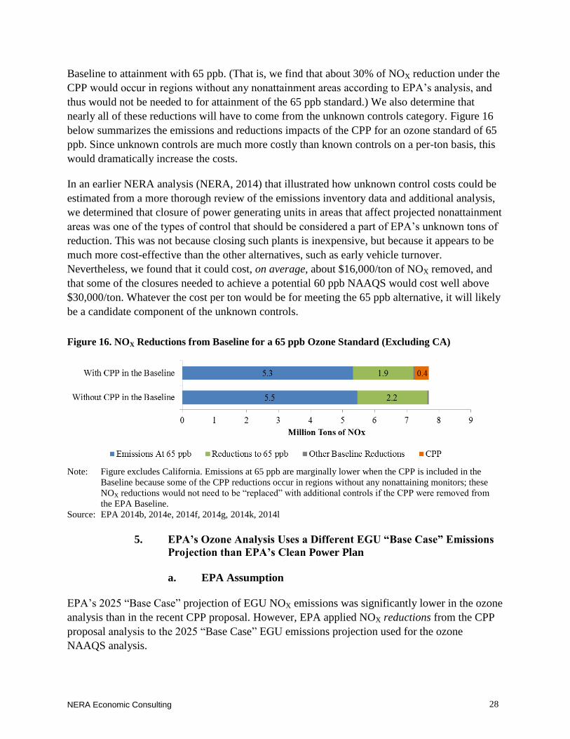
NERA Economic Consulting

28

Baseline to attainment with 65 ppb. (That is, we find that about 30% of NOX reduction under the

CPP would occur in regions without any nonattainment areas according to EPA’s analysis, and

thus would not be needed to for attainment of the 65 ppb standard.) We also determine that

nearly all of these reductions will have to come from the unknown controls category. Figure 16

below summarizes the emissions and reductions impacts of the CPP for an ozone standard of 65

ppb. Since unknown controls are much more costly than known controls on a per-ton basis, this

would dramatically increase the costs.

In an earlier NERA analysis (NERA, 2014) that illustrated how unknown control costs could be

estimated from a more thorough review of the emissions inventory data and additional analysis,

we determined that closure of power generating units in areas that affect projected nonattainment

areas was one of the types of control that should be considered a part of EPA’s unknown tons of

reduction. This was not because closing such plants is inexpensive, but because it appears to be

much more cost-effective than the other alternatives, such as early vehicle turnover.

Nevertheless, we found that it could cost, on average, about $16,000/ton of NOX removed, and

that some of the closures needed to achieve a potential 60 ppb NAAQS would cost well above

$30,000/ton. Whatever the cost per ton would be for meeting the 65 ppb alternative, it will likely

be a candidate component of the unknown controls.

EPA’s Ozone Analysis Uses a Different EGU “Base Case” Emissions 5.

Projection than EPA’s Clean Power Plan

a. EPA Assumption

EPA’s 2025 “Base Case” projection of EGU NOX emissions was significantly lower in the ozone

analysis than in the recent CPP proposal. However, EPA applied NOX reductions from the CPP

proposal analysis to the 2025 “Base Case” EGU emissions projection used for the ozone

NAAQS analysis.

Figure 16. NOX Reductions from Baseline for a 65 ppb Ozone Standard (Excluding CA)

Note: Figure excludes California. Emissions at 65 ppb are marginally lower when the CPP is included in the

Baseline because some of the CPP reductions occur in regions without any nonattaining monitors; these

NOX reductions would not need to be “replaced” with additional controls if the CPP were removed from

the EPA Baseline.

Source: EPA 2014b, 2014e, 2014f, 2014g, 2014k, 2014l

NERA Economic Consulting

29

b. Concern with EPA Assumption

As part of the RIA for the CPP Proposed Rule, EPA projected NOX emissions in both a base case

without the CPP and a policy scenario including the CPP.18

Base case EGU NOX emissions were

1,554,000 tons in 2025 in EPA’s CPP analysis. EPA developed a separate projection of 2025

“Base Case” EGU emissions for this RIA for the ozone NAAQS Proposed Rule using the same

electricity sector model (i.e., IPM) and projected NOX emissions in this ozone “Base Case” of

1,475,000 tons – about 79,000 tons lower than the CPP base case.19

A reduction in base case

EGU emissions has the practical implication of reducing the emission controls needed for

attainment of alternative ozone standards. It is concerning that there is such a significant change

in base case EGU NOX emissions between two recent EPA analyses, particularly given that both

analyses purportedly used version 5.13 of the IPM model, calibrated to the U.S. Energy

Information Administration’s (EIA’s) Annual Energy Outlook 2013 (EIA 2013) demand to

develop their base case projections (EPA 2014h p. 3-46; EPA 2014i p. 86).

As discussed above, we are concerned that the proposed CPP should not be included in EPA’s

Baseline. Even if the CPP were implemented as proposed, the difference between the CPP and

ozone EGU base case projections raises an additional concern about the application of the CPP

projected reductions to EPA’s ozone Base Case. EPA estimated that the CPP would reduce EGU

NOX emissions by about 436,000 tons in 2025 (EPA 2014e and 2014f).20

The estimated

emissions impact of the CPP depends in part on the assumptions in the base case used for EPA’s

CPP analysis. In its ozone analysis, however, EPA subtracted the CPP NOX reductions from the

ozone “Base Case” projection of EGU emissions. Given that the ozone “Base Case” EGU NOX

projection is significantly lower, it may reflect assumptions about additional coal and natural gas

unit retirements or re-dispatch; these differing assumptions could lower the potential NOX

emission reductions attributable to the CPP.

c. Implications of EPA Assumption

We have not been able to determine why EPA’s “Base Case” EGU NOX projection is lower in

EPA’s ozone analysis than in its CPP analysis. If EPA’s “Base Case” EGU NOX emissions were

understated, that understatement would reduce the controls needed for compliance with a new

ozone standard and would cause EPA to understate compliance costs.

Applying the CPP NOX reduction estimates to a lower “Base Case” EGU emissions level likely

overstates the NOX reductions attributable to the CPP (since some of the policy-induced NOX

reductions from EPA’s CPP modeling likely take place in the new “Base Case”). EPA assumed

18

Note that EPA’s ozone analysis distinguished between a “Base Case” (which does not include the CPP) and a

Baseline (which does include the CPP). EPA’s CPP analysis has a single base case.

19 These total EGU emissions figures exclude tribal and offshore data, but include data for California.

20 These NOX reductions are for the Option 1 State CPP scenario, which was used in EPA’s ozone analysis (EPA

2014a p. 3-11).

NERA Economic Consulting

30

the CPP reduces NOX emissions by about 436,000 tons; given the complexities of dispatch

modeling, it is difficult to tell how much this reduction would be diminished as a result of EPA’s

lower “Base Case” NOX projection. Regardless of the magnitude, this inconsistency in EPA’s

analysis understates the controls needed for compliance with a new ozone standard and thus

understates compliance costs.

Concerns Related to EPA’s Calculation of Unknown Control Costs B.

Fully 40% of the estimated tons of reduction needed to attain a standard set at 65 ppb (excluding

California) come from unknown controls, and even using EPA’s approach, this category

accounts for about 73% of the estimated compliance costs. EPA’s approach probably greatly

understated the costs of these unknown controls, as we explain in this section. Along with the use

of the 2025 snapshot to determine the extent of nonattainment and emissions reduction needs, the

way that EPA handled the unknown control costs is probably the other most significant reason to

believe that the RIA is understating the costs of a potential revision to the ozone NAAQS.

EPA Assumed an Average Cost of $15,000 per Ton of Emission 1.

Reductions from Unknown Controls as Its Basic Assumption

a. EPA Assumption

EPA applied a single average cost value of $15,000 per ton to all reductions from unknown

controls. EPA provided the following rationales for taking this simple approach:

EPA’s Science Advisory Board stated in 2007 that, of the three unknown control cost

methods proposed by EPA, “assuming a fixed cost/ton appears to be the simplest and

most straightforward” (EPA 2014a p. 7-27).

The EPA analysis does not include all currently available controls since CoST focuses on

a “limited set of emissions inventory sectors” (EPA 2014a p. 7-12 and 7-28). Unknown

controls could include these currently available (and presumably less expensive) controls

as well as more expensive technologies or more extreme measures.

Historically, EPA has sometimes overestimated the cost of unknown controls and has

failed to account for certain innovations (EPA 2014a p. 7-14).

Future technological innovation can change the pollution abatement cost curve by

making existing controls more efficient or less costly or by introducing new inexpensive

controls (EPA 2014a p. 7-18).

“Learning by doing” can reduce the cost of existing control technologies (EPA 2014a p.

7-20).

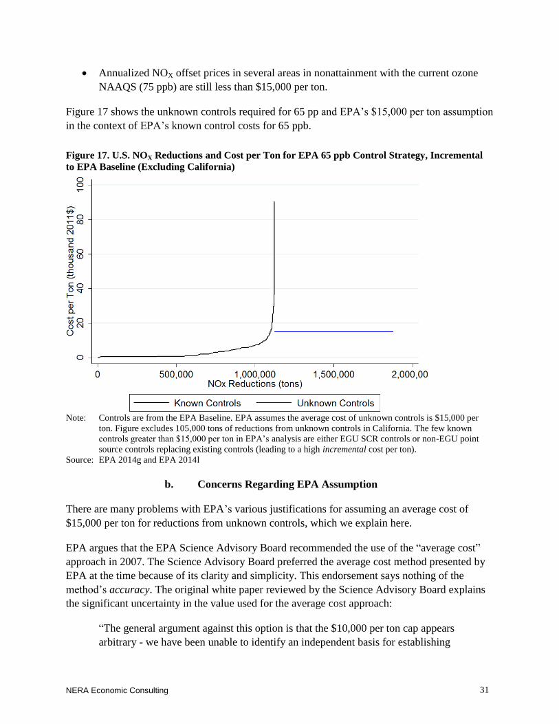
NERA Economic Consulting

31

Annualized NOX offset prices in several areas in nonattainment with the current ozone

NAAQS (75 ppb) are still less than $15,000 per ton.

Figure 17 shows the unknown controls required for 65 pp and EPA’s $15,000 per ton assumption

in the context of EPA’s known control costs for 65 ppb.

b. Concerns Regarding EPA Assumption

There are many problems with EPA’s various justifications for assuming an average cost of

$15,000 per ton for reductions from unknown controls, which we explain here.

EPA argues that the EPA Science Advisory Board recommended the use of the “average cost”

approach in 2007. The Science Advisory Board preferred the average cost method presented by

EPA at the time because of its clarity and simplicity. This endorsement says nothing of the

method’s accuracy. The original white paper reviewed by the Science Advisory Board explains

the significant uncertainty in the value used for the average cost approach:

“The general argument against this option is that the $10,000 per ton cap appears

arbitrary - we have been unable to identify an independent basis for establishing

Figure 17. U.S. NOX Reductions and Cost per Ton for EPA 65 ppb Control Strategy, Incremental

to EPA Baseline (Excluding California)

Note: Controls are from the EPA Baseline. EPA assumes the average cost of unknown controls is $15,000 per

ton. Figure excludes 105,000 tons of reductions from unknown controls in California. The few known

controls greater than $15,000 per ton in EPA’s analysis are either EGU SCR controls or non-EGU point

source controls replacing existing controls (leading to a high incremental cost per ton).

Source: EPA 2014g and EPA 2014l

NERA Economic Consulting

32

$10,000 per ton as a reasonable ceiling on the costs of NAAQS compliance

measures. In addition, there is some evidence that areas are spending more than

this amount on some existing measures…” (812 Project Team 2007, p. 7).

Naturally, some average cost per ton value exists that would approximate actual average

compliance costs; however, the Science Advisory Board review gave no indication of what that

value should be. Additionally, over seven years have passed since this 2007 guidance. EPA

apparently has not prioritized the development of alternative methodologies and continues to rely

on simplicity over improved accuracy in estimating unknown control costs.

During the 2008 and 2010 reviews of the ozone NAAQS, EPA did develop and present estimates

based on an alternative methodology called the “hybrid” approach. This approach involved an

upward-sloping extrapolation from the known control marginal abatement cost curve in order to

estimate the cost of unknown controls. The slope of the extrapolation is dependent on the ratio of

unknown to known control reductions; areas needing a high share of emission reductions from

unknown controls have more rapidly increasing costs per ton for unknown controls. EPA

explained the key advantage of this approach in its 2008 ozone analysis:

“The hybrid methodology has the advantage of using the information about how

significant the needed reductions from unspecified [unknown] control technology are

relative to the known control measures and matching that with expected increasing per

unit cost for going beyond the modeled [known] technology” (EPA 2008 p. 5-13).

Figure 18 illustrates the methodology for this hybrid approach in the context of an example

marginal cost curve for NOX reductions.

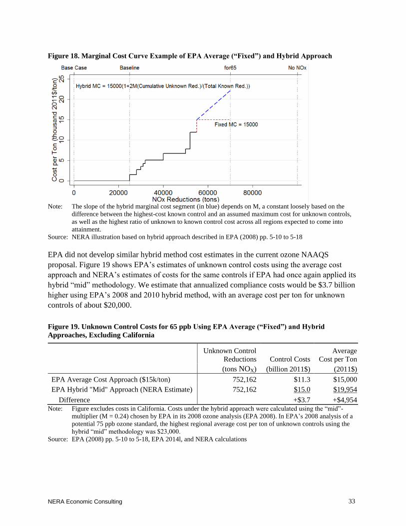
NERA Economic Consulting

33

EPA did not develop similar hybrid method cost estimates in the current ozone NAAQS

proposal. Figure 19 shows EPA’s estimates of unknown control costs using the average cost

approach and NERA’s estimates of costs for the same controls if EPA had once again applied its

hybrid “mid” methodology. We estimate that annualized compliance costs would be $3.7 billion

higher using EPA’s 2008 and 2010 hybrid method, with an average cost per ton for unknown

controls of about $20,000.

Figure 18. Marginal Cost Curve Example of EPA Average (“Fixed”) and Hybrid Approach

Note: The slope of the hybrid marginal cost segment (in blue) depends on M, a constant loosely based on the

difference between the highest-cost known control and an assumed maximum cost for unknown controls,

as well as the highest ratio of unknown to known control cost across all regions expected to come into

attainment.

Source: NERA illustration based on hybrid approach described in EPA (2008) pp. 5-10 to 5-18

Figure 19. Unknown Control Costs for 65 ppb Using EPA Average (“Fixed”) and Hybrid

Approaches, Excluding California

Unknown Control

Reductions Control Costs

Average

Cost per Ton

(tons NOX) (billion 2011$) (2011$)

EPA Average Cost Approach ($15k/ton) 752,162 $11.3 $15,000

EPA Hybrid "Mid" Approach (NERA Estimate) 752,162 $15.0 $19,954

Difference +$3.7 +$4,954

Note: Figure excludes costs in California. Costs under the hybrid approach were calculated using the “mid”-

multiplier (M = 0.24) chosen by EPA in its 2008 ozone analysis (EPA 2008). In EPA’s 2008 analysis of a

potential 75 ppb ozone standard, the highest regional average cost per ton of unknown controls using the

hybrid “mid” methodology was $23,000.

Source: EPA (2008) pp. 5-10 to 5-18, EPA 2014l, and NERA calculations

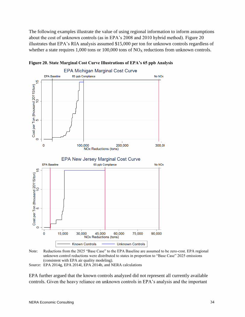
NERA Economic Consulting

34

The following examples illustrate the value of using regional information to inform assumptions

about the cost of unknown controls (as in EPA’s 2008 and 2010 hybrid method). Figure 20

illustrates that EPA’s RIA analysis assumed $15,000 per ton for unknown controls regardless of

whether a state requires 1,000 tons or 100,000 tons of NOX reductions from unknown controls.

EPA further argued that the known controls analyzed did not represent all currently available

controls. Given the heavy reliance on unknown controls in EPA’s analysis and the important

Figure 20. State Marginal Cost Curve Illustrations of EPA’s 65 ppb Analysis

Note: Reductions from the 2025 “Base Case” to the EPA Baseline are assumed to be zero-cost. EPA regional

unknown control reductions were distributed to states in proportion to “Base Case” 2025 emissions

(consistent with EPA air quality modeling).

Source: EPA 2014g, EPA 2014l, EPA 2014b, and NERA calculations

NERA Economic Consulting

35

implications of unknown control costs for the likely impacts of a new ozone standard, EPA

should have made every effort to conduct a truly comprehensive analysis of currently available

known controls. EPA’s argument – that currently available controls not included in the EPA

analysis could be a significant source of additional, inexpensive NOX reductions – is not

substantiated in EPA’s RIA. In our 2014 analysis of a potential 60 ppb ozone standard, we

concluded that “the identity of control options and their costs to achieve the emissions reductions

needed for attainment” was perhaps the most important “gap” for EPA to address in future ozone

analyses (NERA 2014 p. 45); four years after EPA’s ozone NAAQS reconsideration in 2010 and

six years after EPA developed the basic cost and emissions information, EPA has done relatively

little to identify additional controls and address the largest uncertainty in its compliance cost

analyses.

If additional controls do exist that would cost an average of $15,000 per ton, that means there are

controls that must cost a good deal less than that too; but if such less expensive controls were

currently available, presumably they would have already been identified. Based on the

distribution of NOX emissions remaining after the application of EPA’s known controls, it is

difficult to find an emissions source with both a large potential for additional reductions and an

obvious additional control option. Figure 21 shows the emissions remaining in each emission

source category after accounting for known controls. Many of the emissions remaining would be

difficult or impossible for states to control further for the various major source categories.

EGU Sources. Coal and natural gas power plants are already largely controlled as part

of EPA’s known control strategy.

Point Sources. Large point sources are the easiest to regulate and have already been

subject to significant control.

Area Sources. Many area sources such as space heating are highly diffuse, and the stock

is difficult to regulate.

Onroad Sources. Tier 3 vehicle emission standards have significantly reduced projected

onroad emissions, limiting the possibility of significant, inexpensive controls.

Nonroad Sources. One-third of residual nonroad emissions are from freight rail, an

interstate activity not amenable to state-level control. Other nonroad mobile sources like

construction equipment and marine vessels are also difficult to control at the state level.

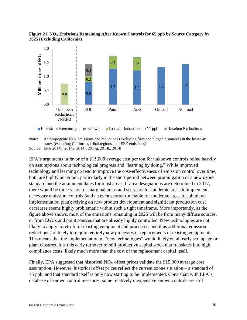
NERA Economic Consulting

36

EPA’s arguments in favor of a $15,000 average cost per ton for unknown controls relied heavily

on assumptions about technological progress and “learning by doing.” While improved

technology and learning do tend to improve the cost-effectiveness of emission control over time,

both are highly uncertain, particularly in the short period between promulgation of a new ozone

standard and the attainment dates for most areas. If area designations are determined in 2017,

there would be three years for marginal areas and six years for moderate areas to implement

necessary emission controls (and an even shorter timetable for moderate areas to submit an

implementation plan); relying on new product development and significant production cost

decreases seems highly problematic within such a tight timeframe. More importantly, as the

figure above shows, most of the emissions remaining in 2025 will be from many diffuse sources,

or from EGUs and point sources that are already highly controlled. New technologies are not

likely to apply to retrofit of existing equipment and processes, and thus additional emission

reductions are likely to require entirely new processes or replacements of existing equipment.

This means that the implementation of “new technologies” would likely entail early scrappage or

plant closures. It is this early turnover of still productive capital stock that translates into high

compliance costs, likely much more than the cost of the replacement capital itself.

Finally, EPA suggested that historical NOX offset prices validate the $15,000 average cost

assumption. However, historical offset prices reflect the current ozone situation – a standard of

75 ppb, and that standard itself is only now starting to be implemented. Consistent with EPA’s

database of known control measures, some relatively inexpensive known controls are still

Figure 21. NOX Emissions Remaining After Known Controls for 65 ppb by Source Category by

2025 (Excluding California)

Note: Anthropogenic NOX emissions and reductions (excluding fires and biogenic sources) in the lower 48

states (excluding California, tribal regions, and EEZ emissions)

Source: EPA 2014b, 2014e, 2014f, 2014g, 2014k, 2014l

NERA Economic Consulting

37

available even in areas with nonattainment problems under the current standard. The relevant

questions are 1) will additional controls be available after this supply of known controls is

exhausted under a tighter ozone standard?, and, 2) at what cost? Until NOX offsets prices reflect

increased demand for unknown controls under a tighter ozone standard, offset prices only

confirm what is already known about the cost of currently available controls.

c. Implications of the Concern

EPA’s assumption on the costs of unknown controls has a major effect on its estimates of the

overall compliance costs of a revised ozone standard. For a potential standard of 65 ppb, EPA

found that about 40% of U.S. NOX reductions (excluding California) would need to come from

unknown controls. However, these unknown controls represent a much larger share of the

estimated compliance costs; for the 65 ppb standard, unknown compliance costs represent about

73% of EPA’s estimate of total annualized compliance costs (excluding California and assuming

a $15,000 average cost per ton for emission reductions from unknown controls).

EPA’s compliance cost estimates were primarily driven by a single, arbitrary assumption about

the average cost of unknown controls, and modifications to that assumption could have a

dramatic effect on the estimated costs and economic impacts of a new ozone standard.

EPA’s Sensitivity Analysis Assumed a Low of $10,000 per Ton and a 2.

High of $20,000 per Ton for Emission Reductions from Unknown

Controls

a. EPA Assumption

EPA noted that the costs of unknown controls are highly uncertain. To reflect the uncertainty,

EPA calculated unknown costs assuming an average cost of $10,000 per ton for the “lower

bound” and an average cost of $20,000 for an “upper bound.”

b. Concerns with EPA Assumption

Given the highly arbitrary nature of EPA’s average cost approach and selection of $15,000 per

ton, EPA’s sensitivity analysis on unknown control costs does little to indicate a range of likely

values. The narrow sensitivity range is inconsistent with both the rest of EPA’s cost analysis and

with prior EPA analyses:

EPA suggests that the accuracy range of the known control costs for non-EGU point and

area sources is plus or minus 30%, yet EPA’s sensitivity analysis of unknown control

costs is performed at a range of only plus or minus 33% (EPA 2014a p. 7-39).

The hybrid “mid” approach presented alongside the average cost method estimates in

EPA’s 2008 and 2010 ozone analyses would imply an average cost per ton of about

$20,000 in the current analysis (the “upper bound” of EPA’s cost sensitivity).

NERA Economic Consulting

38

The 2007 white paper on unknown control costs that was reviewed by the Science

Advisory Board suggested possible assumptions that were outside EPA’s $10,000 to

$20,000 per ton sensitivity range. For example, “One option would be to use the effective

marginal cost of I/M controls…between $25,000 and $30,000 per ton for both VOC and

NOX reductions” (812 Project Team 2007, p. 7).

EPA’s only rationale for its cost sensitivity assumptions was, “This range is inclusive of the

annualized NOX offset prices observed in recent years in the areas likely to need unknown

controls to achieve the proposed standard, and if anything, suggests the central estimate of

$15,000/ton is conservative” (EPA 2014a p. 7-30). As discussed above, recent NOX offset prices

are not indicative of the average cost of future unknown controls, and they certainly do not

reflect the uncertainty in estimating future average control costs. The cost range of EPA’s

sensitivity analysis and the declaration that EPA’s primary unknown control cost estimate is

“conservative” are unfounded.

c. Implications of EPA Assumption

Given indications of significant uncertainty in known control costs and the significant reliance on

unidentified control measures to comply with a new ozone standard, EPA significantly

understates the uncertainty in unknown control costs, and therefore significantly understates the

uncertainty in total control costs.

Summary of Concerns C.

All seven of the concerns summarized in this section point to a conclusion that the EPA RIA

understated the potential costs—including the range of potential costs—of meeting a more

stringent ozone standard. Four of these concerns seem in our judgment likely to lead to a major

understatement of compliance costs.

EPA used a 2025 “snapshot” to estimate incremental attainment needs, but

nonattainment designations and attainment deadlines are earlier. This assumption likely

leads to a major understatement in the number of areas that will be in nonattainment as

well as an understatement of the number of tons needed to be reduced compared to

Baseline emissions and timing of the spending. Areas designated as marginal or moderate

would likely have attainment dates around the end of 2020 and 2023, respectively, and

would incur costs before 2025—costs that are disregarded (by assumption) in EPA’s

analysis. (Our assessment does not consider the complications of potential

reclassifications of individual non-attainment areas.)

EPA included the proposed Clean Power Plan (CPP) in the Baseline. EPA’s inclusion of

CPP emission reductions is not only inconsistent with its standard practice of only

including promulgated regulations, but such a deviation from standard procedure is

particularly unjustified given the enormous uncertainty in what carbon limits may

NERA Economic Consulting

39

actually be applied and how states would comply, and hence what NOX emission

reductions might actually occur as a result of EPA regulation of carbon emissions from

existing electricity generating units. Without the proposed CPP in the Baseline, at least an

additional 300,000 tons of NOX reductions would be required for the 65 ppb standard,

leading to a substantial increase in the estimated compliance costs.

EPA assumed a constant value of $15,000 per ton for all unknown emission reductions.

Controls that EPA referred to as unknown (i.e., for which no compliance controls are

identified) represent about 40% of EPA’s estimated tons and about 73% of EPA’s

estimated costs to attain a 65 ppb ozone standard (excluding California). As one

indication of the importance of this single assumption, we calculated that unknown

control costs would increase by about $3.7 billion per year (i.e., from $11.3 billion to

$15.0 billion, excluding California) if EPA had used an alternate methodology presented

in its own most recent prior ozone NAAQS cost assessment in 2010. Changing just this

one aspect of the EPA methodology would lead to a total cost estimate of $19.2 billion to

achieve a 65 ppb ozone standard (excluding California).

EPA assumed an uncertainty band for unknown costs of $10,000 to $20,000 per ton. This

arbitrary range seems likely to understate substantially the potential compliance costs.

Given that unknown controls would have to reduce emissions from many diffuse area or

mobile sources—since point sources are already highly controlled—the cost per ton

could be substantial (e.g., requiring early turnover of still productive capital stock such as

residential or commercial heating).

In summary, our evaluation suggests that EPA has understated the potential compliance costs—

including their likely range—of meeting a more stringent ozone standard. The costs of achieving

a more stringent ozone standard could be substantially greater than even the very substantial

costs EPA has estimated.

NERA Economic Consulting

40

IV. REFERENCES

NERA Economic Consulting (NERA). 2014. “Assessing Economic Impacts of a Stricter

National Ambient Air Quality Standard for Ozone.” July.

U.S. Energy Information Administration (EIA). 2013. Annual Energy Outlook 2013.

U.S. Environmental Protection Agency (EPA). 2008. Final Ozone NAAQS Regulatory Impact

Analysis. March. http://www.epa.gov/ttn/ecas/regdata/RIAs/452_R_08_003.pdf.

U.S. Environmental Protection Agency (EPA). 2010. Supplemental Regulatory Impact Analysis

(RIA) for the Reconsideration of the 2008 Ozone National Ambient Air Quality Standard

(NAAQS). http://www.epa.gov/ttn/ecas/regdata/RIAs/s1-supplemental_analysis_full.pdf.

U.S Environmental Protection Agency (EPA). 2014a. Regulatory Impact Analysis (RIA) of the

Proposed Revisions to the National Ambient Air Quality Standards (NAAQS) for Ground-Level

Ozone. http://www.epa.gov/ttnecas1/regdata/RIAs/20141125ria.pdf

U.S Environmental Protection Agency (EPA). 2014b. 2011 and 2025 NOX Emissions County

Sector Comparison.

ftp://ftp.epa.gov/EmisInventory/2011v6/ozone_naaqs/reports/2011ef_2025ef_county_sector_co

mparison_NOX.xlsx

U.S Environmental Protection Agency (EPA). 2014c. 2011 and 2025 VOC Emissions County

Sector Comparison.

ftp://ftp.epa.gov/EmisInventory/2011v6/ozone_naaqs/reports/2011ef_2025ef_county_sector_co

mparison_VOC.xlsx

U.S Environmental Protection Agency (EPA). 2014d. 2011, 2018, and 2025 Emissions State

Sector Comparison.

ftp://ftp.epa.gov/EmisInventory/2011v6/ozone_naaqs/reports/2011ef_2018ef_2025ef_state_secto

r_comparison.xlsx

U.S Environmental Protection Agency (EPA). 2014e. Proposed Clean Power Plan: IPM State-

Level Emissions, Base Case. http://www.regulations.gov/#!documentDetail;D=EPA-HQ-OAR-

2013-0602-0224

U.S Environmental Protection Agency (EPA). 2014f. Proposed Clean Power Plan: IPM State-

Level Emissions, Option 1 State. http://www.regulations.gov/#!documentDetail;D=EPA-HQ-

OAR-2013-0602-0228

U.S Environmental Protection Agency (EPA). 2014g. O3 NAAQS RIA Control Strategy Results

NOX Controls for 65ppb Analysis Incremental to Baseline.

http://www.regulations.gov/#!documentDetail;D=EPA-HQ-OAR-2013-0169-0015

NERA Economic Consulting

41

U.S Environmental Protection Agency (EPA). 2014h. Regulatory Impact Analysis for the

Proposed Carbon Pollution Guidelines for Existing Power Plants and Emission Standards for

Modified and Reconstructed Power plants. http://www2.epa.gov/sites/production/files/2014-

06/documents/20140602ria-clean-power-plan.pdf

U.S Environmental Protection Agency (EPA). 2014i. Technical Support Document (TSD):

Preparation of Emissions Inventories for the Version 6.1, 2011 Emissions Modeling Platform.

http://www.epa.gov/ttn/chief/emch/2011v6/2011v6.1_2018_2025_base_EmisMod_TSD_nov201

4_v6.pdf

U.S. Environmental Protection Agency (EPA). 2014j. 2017 and Later Model Year Light-Duty

Vehicle Greenhouse Gas Emissions and Corporate Average Fuel Economy Standards. Federal

Register 77(199): pp 62624-63200. http://www.gpo.gov/fdsys/pkg/FR-2012-10-15/pdf/2012-

21972.pdf

U.S Environmental Protection Agency (EPA). 2014k. Updated 2014 O3 NAAQS RIA NOx

Control Strategy Results – 75 ppb. http://www.regulations.gov/#!documentDetail;D=EPA-HQ-

OAR-2013-0169-0035

U.S Environmental Protection Agency (EPA). 2014l. Emission Reductions Beyond Known

Controls. http://www.regulations.gov/#!documentDetail;D=EPA-HQ-OAR-2013-0169-0032

Second Section 812 Prospective Project Team (812 Project Team). 2007. Methods to Estimate

Costs of: (1) Unidentified Control Measures to meet NAAQS Requirements and (2) Direct Costs

when Mark-up Factors are Present.

http://www.epa.gov/cleanairactbenefits/mar07/cost_estimation.pdf

200 Clarendon Street

11th Floor

Boston, MA 02116

617-927-4500

1255 23rd Street NW

Suite 600

Washington, DC 20037

202-466-3510

www.nera.com