1

A memory time varying ARFIMA model for weather derivative pricing1

Massimiliano Caporin1 and Juliusz Preś2

1“Marco Fanno” Department of Economics

University of Padova Via del Santo, 33, 35123 Padova, Italy

massimiliano.caporin@unipd.it

2Institute of Economy and Management Szczecin University of Technology

Al. Piastow, 48, 70311 Szczecin, Poland jpres@ps.pl

VERY PRELIMINARY AND PARTIAL VERSION

Abstract. We present a generalisation of the long memory ARFIMA models introducing time-varying memory coefficients. The model satisfies the empirical evidence of changing memory observed in average temperature series and can provide useful improvements in the forecasting, simulation and pricing issues related to weather derivatives. We provide an application related to the forecast and simulation of temperature indices used for pricing of weather options.

Keywords: weather derivatives, long memory, time varying long memory, derivative pricing, forecast evaluation. JEL Codes: C22, C15, C53, G10, G13.

1 Introduction

It is well-known that the weather may have a crucial impact on business activities. This effect is very relevant even at the macroeconomic level. In fact, as evidenced by Ku (2001), the U.S. Department of Commerce estimates that the weather affects nearly 70% of U.S. companies, and almost 22% of U.S. GDP. McWilliams (2004) demonstrates similar results for the European Economy.

In the last ten years the need for hedging and offsetting weather-related risks and the increasing development of financial markets contributed to the creation of the weather derivative market. In this new market, financial intermediaries and private company exchange derivative contracts where the underlying asset is a weather-related variable (such as the average daily temperature, the wind speed, the rainfall). By now, the largest part of the exchanged weather contracts is linked to the temperature values. The financial literature provided several studies presenting the general pricing problems of weather derivatives, see Geman (1999), Cao and Wei (2000, 2003), Zeng (2000), Alaton, Djehiche and Stillberger (2002), Dischel (2002), Brix, Jewson and Ziehmann (2002), Jewson and Brix (20005) among an increasing number of contributions. The most interesting aspect is, however, the development of appropriate methods for forecasting the underlying weather variables and pricing the associated weather derivatives. Some examples are given by Roustant et al. (2003), Campbell and Diebold (2005), Hamisultane (2006a), Taylor and Buizza (2006) that focus on the daily modelling and forecasting of temperatures.

More recently, some authors evidenced the presence of long memory in temperature series, see Caballero, Jewson and Brix (2002), Hamisultane (2006b), among others. This empirical finding is well-know and deeply analysed in the statistical and econometric literature. The first studies dates back to the beginning of the 80’s with the seminal papers by Granger (1980, 1981), Granger and Joyeux (1980), Hosking (1981) and then to the contributions of Sowell (1992a,b), among others. The traditional ARFIMA models have been applied in different economic areas such as foreign exchange, Cheung (1993), Gil-Alana and Toro (2002) and Beine and Laurent (2003), stock markets, Lo (1991), Ding, Granger and Engle (1993), Mills (1993), Cheung and Lai (1995), output, Diebold and Rudebush (1989), inflation, Hassler and Wolters (1995), Baillie, Chung and Tieslau (1996) and Doornik and Ooms (2004), monetary aggregates, Porter-Hudak (1990), interest rates, Iglesias and Phillips (2005) and Couchman, Gounder and Su (2006), forward

1 The first author acknowledges financial support from the Italian Ministry of University and Research project PRIN2006 “Econometric analysis of interdependence, stabilisation and contagion in real and financial markets”. Both authors acknowledge financial support from the Europlace Institut of Finance under the project “Understanding and modelling weather derivatives: a statistical and econometric investigation”

2

premium, Baillie and Bollerslev (1994), electricity prices, Koopman, Ooms and Carnero (2007), among others. We also cite the srveys by Baillie (1996), Bhardway and Swanson (2006) and the book by Beran (1994). There are also some contributions relating long memory to atmospherical or physical elements: hydrology, Hosking (1984), climatology, Baillie and Chung (2002), temperature Smith (1993) and Moreno (2003).

Following this strand of the literature, this paper presents a new approach for long-memory modelling of temperature series. Temperature series have been analysed with the ARFIMA model, see Caballero and Jewson (2002), Caballero et al. (2002) and Hamisultane (2006b). However, there are some evidences that the memory degree is not stable over time, Katz (1996), Katz and Parlange (1998), and Caballero, Jewson and Brix (2002). The previous authors also evidence that the missing inclusion of this feature may provide under- or over- estimates of the process variance with relevant impacts on the derivative pricing. In this paper we propose a variation of the traditional ARFIMA model allowing for changes in the memory coefficient over time. In particular, we present a model where the memory behaviour is monthly-specific. Given the relevance of temperature-related weather derivatives, we show that the proposed model provide better fittings on several temperature based series comparing it with the traditional ARFIMA. We provide also a forecast based comparison and a pricing example.

In the following section we present the main problems and pricing approaches in the weather derivatives market. Section 3 introduces the Time-Varying ARFIMA model and deals with model estimation, forecast and simulation. The empirical examples are included in Section 4 where we provide a model comparison based on forecast and weather derivative pricing. Finally, Section 5 concludes. 2 Weather Risks, Weather Derivatives and Pricing Issues

Usually, the label “weather risk” identifies the financial exposure that a business may have to weather events such as heat, cold, snow, rain or wind (Clemmons, 2002). Among the most weather-sensitive sectors we may include, Energy (sensible to excessive heating or cooling periods), Agriculture, Construction (extreme weather conditions may reduce the building processes but also extreme weather events may have impacts, such as hurricanes and storms), Grocery, Brewing, Entertainment. The relevant weather risk exposition of many economic activities and the corresponding need of hedging or offsetting these risks given rise to the diffusion of weather related insurance contracts. The strong link between insurance companies and the financial markets and the search for the most efficient methods for covering weather risks, promoted the inclusion and diffusion of weather related contracts in the capital markets, see Foster (2003) and Van Lennep et al. (2004). Certainly this fact had a significant contribution in development of weather derivatives market which started in the 90s in the United States as an effect of the deregulation of the energy sector. Who transacted the first weather contract is unclear, but in 1996 Aquila entered into a deal with Consolidated Edison whose aim was to protect the last one against a cool August. One year later Enron and Kansas-based Koch Industries made a publicized deal where the payoff was based on the Heating Degree Days (HDD) temperature index. In the following years, the sudden growth of this market induced the Chicago Mercantile Exchange (CME) to launch around 1999 weather futures and options. At the beginning, the CME were quoting only temperature indices for few major US cities (weather events are in fact, localisation specific). Later, the available contracts and localisations start increasing and, at this time there are more than 70 different weather contracts in trade (including temperature, snowfall and frost) for 35 different locations in the world. After ten years, thanks to the existence of different weather anomalies and to the start of deregulation processes in the other countries, this market grows rapidly attracting the interest of many participants, as evidenced by the annual reports of the Weather Risk Management Association (WRMA henceforth). The 2006/2007 report indicates that the value of the weather derivative market reach 25 USD blns (WRMA Survey, 2007).

Notably, most companies that belong to above weather-exposed sectors are subject to (mainly or in significant part) the risk of unfavourably air temperature. Such conclusion can be also directly drawn from the above mentioned WRMA annual reports. In fact, more than 90% of all trades done in recent years were referred only to temperature based contracts. For this reason, this paper focuses only on modelling and pricing of weather derivatives based on air temperature. The extension of our modelling approach to additional weather derivatives may constitute an interesting area for future contributions.

2.1 Weather Derivatives

A weather derivative is a financial contract where the underlying asset is a weather index or a set of weather

indices. The type of available contract spans the traditional taxonomy of derivatives including also exotic types. Weather derivatives are mainly traded in Over-The-Counter markets (OTC) and only recently in exchange markets, but only at the Chicago Mercantile Exchange (CME). Other exchanges like LIFFE, Deutsche Börse or Powernext attempted to launch similar contracts, but the local interest was too small and trades have been suspended (Nicholls, 2004). Currently the CME quotes temperature futures and options of these futures (European exercise style) for selected major cities of US, Canada, Europe and Japan. Contracts

on other weather indices are quoted only for few locations, for example the Frost Days index Snowfall index for New York and Boston. For US localizations two temperature indices are normally uses: Heating Degree Days (HDDs) and Cooling Degree Days (CDDs).

The HDD Index is used during the heating season (October sum of daily HDD values, which in turn are calculated as

obtained from daily maximum and minimum temperature. The index is evaluated as the discrepancy from a baseline temperature which is fixed at 65° Fahrenheit degrees.The CDD Index is used in warm months (cooling is on) and is calculated similarly to the HDD, cumulating daily valuesof cooling degrees, defined as

only while for Canada and Europe, Celsius degrees are used with a baseline temperature of 18ºC. Given the colder climate reported in Europe and Canada compared to the US localizations, the CDD index is substituted by the CAT (Cumulated Average Temperature) indcontract duration the daily values of

For Japanese localizations (Osaka and Tokio) a further index is use, the MAT (Monthly Average Temperature), calculated as the average of the hderivatives are priced considering the expected values that one of the previous indices at the contract maturity.

2.2 Pricing Approaches

As evidenced by Brix, Jewson and Ziehmann (20

of weather contract for three main reasons. The first one is obviousthis information in order to implement a reasonable trade. Tinstruments and arises from the need of building dynamic hedgefrom the internal rules of a given company scenarios for the possible values of the contracts in the future,

The best method to obtain information about present value of price in the market. However, at the present time, U.S. In all other cases, a suitable model should be used Considering the unique features of weather derivatives, standard model of arbitrwell-know Black and Scholes (1973) (1998). First, portfolio replication is in this case impossibleit is traded. Furthermore, in the BlackBrownian motion while the nature of evidenced by Brix, Jewson, Ziehmann (2005) or Campbell, Diebold (2005)been proposed in the mathematical finance literatureValor (2001), Brody, Syroka and Zervos (2002)(2003), Benth and Saltyté-Benth (2005), suggest the use of a close substitute of the underlying in the pricing equation, related to the limited liquidity of weather contracts that could have serious consequences on the pricing process.arguments favoured the implementation

Actuarial pricing consists on available, weather forecasts, see Cao and Wei (2000, 2003), Zeng (2000), Davis (2001), Brix, Jewson, Ziehmann (2002) and Roustand, Laurent, Bay and Carraro (2003)from such a distribution as a discountedexample). Within the actuarial approach, value densities: Historical Burn Analysis, Index Modelling and Daily Modelling.contract price simply using the historical tracks of weather indices withModelling (an extension of the Burn Analysis) adds a distributional hypothesis to the historical weather indices, which is more suitable for the identification of the tails,Brix (2000). The biggest advantages of both methods are and the possibility of pricing any weather contracts. index and not the underlying weather variable historical observations for the pricing processvariables, as in the case of HDD and CDD indices for the temperature)appropriate choice of weather indices distribution

Some of above drawbacks, especially in the pricingDaily Modelling (Brix, Jewson, Ziehmann, 2002). that this approach does not analyse directly the weather indices but tmeteorological forecasts related to temperature values cnatural way. Basically, this approach tries to identify

max 65 ,0t tCDD x F= −

tx

on other weather indices are quoted only for few locations, for example the Frost Days index Snowfall index for New York and Boston. For US localizations two temperature indices are normally uses: Heating Degree Days (HDDs) and Cooling Degree Days (CDDs).

The HDD Index is used during the heating season (October – April) and is calculated as a monthly or seasonal which in turn are calculated as , where

obtained from daily maximum and minimum temperature. The index is evaluated as the discrepancy from a baseline h is fixed at 65° Fahrenheit degrees.

The CDD Index is used in warm months (cooling is on) and is calculated similarly to the HDD, cumulating daily values. Note that the Fahrenheit degrees are used for US localizations

while for Canada and Europe, Celsius degrees are used with a baseline temperature of 18ºC. Given the colder climate reported in Europe and Canada compared to the US localizations, the CDD index is substituted by the CAT (Cumulated Average Temperature) index during summer months. The CAT index is evaluated cumulating over the

.

For Japanese localizations (Osaka and Tokio) a further index is use, the MAT (Monthly Average Temperature), calculated as the average of the hourly temperatures over the contract duration. In practice, all weather derivatives are priced considering the expected values that one of the previous indices at the contract maturity.

Brix, Jewson and Ziehmann (2005), weather market participants want to know the real value of weather contract for three main reasons. The first one is obvious, because both of the demand and supply sides need

in order to implement a reasonable trade. The second motivation refers mainly to writers of such from the need of building dynamic hedges for all contracts in short position. The last one results

given company and may be related to the periodic assets valuation, contracts in the future, for tax and law restrictions.

The best method to obtain information about present value of weather-related instrument is to at the present time, this can be done only for some localization in the world, mostly in the

other cases, a suitable model should be used, VanderMarck (2003). unique features of weather derivatives, standard model of arbitrage

pricing framework, seems to be inadequate for a number of reasons. First, portfolio replication is in this case impossible given that the underlying variable is not a financia

n the Black-Scholes formula the price of the underlying instrument follows a geometric Brownian motion while the nature of the weather variable process may be very different and more complex

wson, Ziehmann (2005) or Campbell, Diebold (2005) for air temperaturebeen proposed in the mathematical finance literature, see Dornier and Querel (2000), Davis (2001),

Brody, Syroka and Zervos (2002), Henderson (2002), Jewson (2002), Benth (2003), Benth (2005), among others. In order to solve the market incompleteness, some

the use of a close substitute of the underlying in the pricing equation, but this give rise to a further problem related to the limited liquidity of weather contracts that could have serious consequences on the pricing process.

implementation of alternative pricing approaches, such as the actuarial Actuarial pricing consists on forecasting the distribution of contract outcomes using historical data and,

Cao and Wei (2000, 2003), Zeng (2000), Davis (2001), Augros and Moreno (2002), and Roustand, Laurent, Bay and Carraro (2003). The contract p

distribution as a discounted expected value plus some risk loading factor (see Henderson, 2002, for an Within the actuarial approach, there are three different methods for the estimation

Historical Burn Analysis, Index Modelling and Daily Modelling. Historical Burn Analysis historical tracks of weather indices without any modelling approach. Differently,

the Burn Analysis) adds a distributional hypothesis to the historical weather indices, which is more suitable for the identification of the tails, and evaluates contracts using Monte Carlo simulations

. The biggest advantages of both methods are their simplicity, the limited efforts needed for all possibility of pricing any weather contracts. However, they also have many drawbacks:

index and not the underlying weather variable (Nelken, 2000), and, more seriously, they use a limited number of historical observations for the pricing process (weather indices are generally based on an aggregation of weather

the case of HDD and CDD indices for the temperature). This fact has distribution and on the size of parameter estimation’s error.

Some of above drawbacks, especially in the pricing of temperature-related contracts, can be Daily Modelling (Brix, Jewson, Ziehmann, 2002). At first, the amount of data used in estimation is much biggerthat this approach does not analyse directly the weather indices but the underlying weather vmeteorological forecasts related to temperature values could be incorporated into the pricing process in easy and quite

tries to identify a model that is able to replicate the historical

{ }max 65 ,0t tCDD x F°= −

3

on other weather indices are quoted only for few locations, for example the Frost Days index for Amsterdam and the Snowfall index for New York and Boston. For US localizations two temperature indices are normally uses: Heating

s calculated as a monthly or seasonal where is average temperature

obtained from daily maximum and minimum temperature. The index is evaluated as the discrepancy from a baseline

The CDD Index is used in warm months (cooling is on) and is calculated similarly to the HDD, cumulating daily values Note that the Fahrenheit degrees are used for US localizations

while for Canada and Europe, Celsius degrees are used with a baseline temperature of 18ºC. Given the colder climate reported in Europe and Canada compared to the US localizations, the CDD index is substituted by the CAT

ex during summer months. The CAT index is evaluated cumulating over the

For Japanese localizations (Osaka and Tokio) a further index is use, the MAT (Monthly Average ourly temperatures over the contract duration. In practice, all weather

derivatives are priced considering the expected values that one of the previous indices at the contract maturity.

eather market participants want to know the real value because both of the demand and supply sides need

tion refers mainly to writers of such for all contracts in short position. The last one results

periodic assets valuation, the creation of different

instrument is to observe their can be done only for some localization in the world, mostly in the

age-free pricing, such as the seems to be inadequate for a number of reasons, Dischel given that the underlying variable is not a financial asset nor

Scholes formula the price of the underlying instrument follows a geometric different and more complex, as

for air temperature. Some solutions have Dornier and Querel (2000), Davis (2001), Torro, Meneu and

Benth (2003), Jewson and Zerovs In order to solve the market incompleteness, some authors

but this give rise to a further problem related to the limited liquidity of weather contracts that could have serious consequences on the pricing process. These

of alternative pricing approaches, such as the actuarial one. using historical data and, if Augros and Moreno (2002),

The contract price is then obtained (see Henderson, 2002, for an

different methods for the estimation and forecast of contract Historical Burn Analysis evaluates the

out any modelling approach. Differently, Index the Burn Analysis) adds a distributional hypothesis to the historical weather indices, which

Carlo simulations, Jewson and the limited efforts needed for all calculations

, they also have many drawbacks: they model the weather , and, more seriously, they use a limited number of

(weather indices are generally based on an aggregation of weather . This fact has a relevant impact on the

and on the size of parameter estimation’s error. contracts, can be overcome using

, the amount of data used in estimation is much bigger, given he underlying weather variables and,

pricing process in easy and quite historical meteorological data.

tx

4

Then, by Monte Carlo simulations, it estimates the future evolution of the underlying weather variables, of the weather indices based on these variables and of the contract payoff distribution. The Daily Modelling could be the preferred solution, clearly conditionally on the correct specification of the adopted model, Jewson (2004). However, even this approach presents some limitations. In fact, weather variables may present periodic patterns (associated to the seasonal evolution of the weather) and long memory, Alaton et al. (2001), Caballero et al. (2001), Jewson and Caballero (2002). While the simple inclusion of a seasonal patter (which we may expect on a weather related variable) generally creates limited statistical and computational problems, the presence of long-term correlation in weather time series greatly increases the complexity of the analysis. Traditional models can be used, taking advantage of the several contributions, starting from the already mentioned researches of Granger (1980, 1981) and Hosking (1981). However, the most recent findings evidenced that long memory may be present both in the mean and in the variances, while variances may also present periodic components, Moreno (2003) and Taylor and Buizza (2006). Finally, the degree of long memory could vary over time according to the evolution of the seasons, Katz (1996), Katz and Parlange (1998) and Caballero, Brix and Jewson (2001). The misspecification of the memory behaviour of weather-related variables may have relevant impact on the pricing process of the weather derivatives, as mentioned by the previously cited authors. The main contribution of this paper is to provide a theoretical model that includes the empirical evidence of a time varying long memory coefficient in the mean. This new model is introduced in the following section. 3 An ARFIMA Model With Time Varying Memory

The air temperature represents the underlying variable for the largest part of the weather derivatives traded in the world market. The temperature series are therefore the most analysed in the financial literature related to weather derivatives. We contribute to this research field by proposing a new long memory model, the Time-Varying ARFIMA (TV-ARFIMA) whose main property is the time varying nature of the model coefficients. This model feature implements the empirical findings of changing memory behaviour observed on air temperature series previously evidenced. The model we propose for the average temperature index is composed by different building blocks: a

periodic function in the mean ; an ARFIMA structure on the demeaned index; a periodic function in the variances

; finally, a GARCH structure in the variances. The general model may be represented as follows:

( )( ) ( ) ( ) ( )( ) ( )

1

~ 0,1

d t

t t t t

t t t t

L L x t L

s t z z iid D

µ ε

ε σ

Φ − − = Θ

= (1)

where obeys a GARCH process, the innovations are independently and identically distributed according to an

un-specified density with zero mean and unit variance, and the ARFIMA model coefficients may be time-varying. In the following we describe the various building blocks of our model motivating our choices.

The index is characterised by a strong periodic pattern in the mean, associated to the evolution of the

seasons over the year, see Jewson and Caballero (2002). Following standard practice in this framework (see Campbell and Diebold, 2005, among others) we model the periodic deterministic mean component as follows

( )01 1 1

2 2cos sin

365 365

QM Pi

t i j l t ti j l

jt ltx t y t y

π πα α δ γ µ= = =

= + + + + = +

∑ ∑ ∑ (2)

where is the ‘seasonally adjusted’ series (which may present both autocorrelation and heteroskedasticity). The

periodic pattern contains two main elements, a polynomial trend and a pure periodic wave obtained by the combination of a set of harmonics.

We then model the series with an ARFIMA-type structure that tries to match the changing memory

behaviour observed in average temperature values. As we previously observed, the empirical behaviour of the historical temperature indices suggests that the memory level may change over the year. We assume that the memory level change over sub-periods of the year. Define by a partition of the year into S sub-periods, which we call

‘seasons’ for simplicity. Note that S may be different from 4 and in the following we will assume that S=12 and that each element in the partition identifies a specific month of the year. Given a time index, we can assign each point in time to one and only one element of the partition (the sub-periods do not overlap and they cover the entire year). We propose the following parameterisation for , the stochastic mean component of the temperature index, which we call

Time-Varying ARFIMA (TV-ARFIMA):

tx

( )tµ

( )s t

2tσ tz

tx

ty

ty

{ }1 2, ,... ST T T=F

ty

( )( ) ( )

( )

( )( )

( )

1 1 1 1 1 1

2 2 2 2 2 2

1

td

t t t t

t t t

S S S S S S

L L y L

d t T L t T L t T

d t T L t T L t Td L L

d t T L t T L t T

εΦ − = Θ

∈ Φ ∈ ∈ Φ ∈ Θ ∈ = Φ = Θ =

∈ Φ ∈ Θ ∈

⋮ ⋮ ⋮ ⋮ ⋮ ⋮

where is the time varying memory coefficient,

the lag operator and is an innovation process

different values depending on the actual period of year. The time varying ARMA components follow a similar structure with a further character, we do not restrict their order to be the same over all elemen

The following conditions are sufficient for ensuring stationary and invertibility of the mean model:i) the memory coefficients are all lower than ½,

ii) the roots of all AR polynomials are outside the unit circle;iii) the roots of all MA polynomials are outside the unit circle.

The traditional ARFIMA(p,d,q) model independence for the memory coefficient and the

and we obtain

( )( )1d

L L y LΦ − = Θ

If the subsets included in the partition as a special threshold model where the thresholds are associated to the time index.

Furthermore, given that we assumeover years), our model may be represented in a companion form using a matrix of dummy variables. In fact, the memory coefficient may be written as

, ,...t t Sd d d d= =S d d

and is a row selection vector. Then,

associated to one of the elements of representations may be obtained for the order to account for the possible different orders over the seasons.

The model may be related to the recent contributions ofthe authors use an ARFIMA model where the memory coefficient is driven by a Markov chain. In order to solve the computational problems of model estimation and inference the Markov chain is assumed to be observable. Our model may be a special case of the previous approach where the Markov chain is observable and associated to the months of the year. We have not considered the direct Markov switching extension of our model for computational reasons. Given that the main interest in weather derivative pricing is asand the corresponding values within each month of the daily average temperature, we should have used a MS model with 12 states. The number of states is itself relevant and may create computationaldealing with a long memory model that requires long time series for providing reliable estimates. Joining the two aspects may result in a very complex model from a computationaon the asymptotic behaviour of coefficient estimates.

Notably, our model includes a special ARMA representation with time varying polynomials when

We now define the structure of the

elements: a periodic component related to the changing weather risk over time; a purely heteroskedastic component with a GARCH-type structure. Following the contributions of Andersen and Bollefrom Taylor and Buizza (2006), we model

(t t ts t zε σ=

td

tε

( ) ( )t L LΘ = Θ

tS

F

( )

( )( )

( )

1 1 1 1

2 2 2 2 t t t

S S S S

L t T L t T

L t T L t Td L L

L t T L t T

Φ ∈ Θ ∈ Φ ∈ Θ ∈ = Φ = Θ =

Φ ∈ Θ ∈

⋮ ⋮ ⋮ ⋮

(3)

memory coefficient, and are two AR and MA time varying

is an innovation process. The coefficient is of time varying nature because it assumes

different values depending on the actual period of year. The time varying ARMA components follow a similar structure with a further character, we do not restrict their order to be the same over all elements in .

The following conditions are sufficient for ensuring stationary and invertibility of the mean model:i) the memory coefficients are all lower than ½, ;

ii) the roots of all AR polynomials are outside the unit circle; nomials are outside the unit circle.

he traditional ARFIMA(p,d,q) model is nested in our representation under the assumption of time the memory coefficient and the model polynomials. In fact, if we assume that

( )d

t tL L y L εΦ − = Θ (4)

If the subsets included in the partition represent consecutive periods, the model in (3as a special threshold model where the thresholds are associated to the time index.

Furthermore, given that we assume the stability over time of the partition structure (the subsets do not change over years), our model may be represented in a companion form using a matrix of dummy variables. In fact, the

{ }1 2 , ,...t t Sd d d d ′= =S d d (5)

Then, is an S-column matrix of dummies.

and identifies one of the seasons over the entire sample.representations may be obtained for the AR and MA polynomials with a proper definition of the parameter vectors in order to account for the possible different orders over the seasons.

he model may be related to the recent contributions of Haldrup and Nielsen (2006a,b) authors use an ARFIMA model where the memory coefficient is driven by a Markov chain. In order to solve the

computational problems of model estimation and inference the Markov chain is assumed to be observable. Our model us approach where the Markov chain is observable and associated to the months of

We have not considered the direct Markov switching extension of our model for computational reasons. Given that the main interest in weather derivative pricing is associated to monthly values of the HDD, CDD and CAT indices, and the corresponding values within each month of the daily average temperature, we should have used a MS model

. The number of states is itself relevant and may create computational problems. Furthermore, we are dealing with a long memory model that requires long time series for providing reliable estimates. Joining the two

may result in a very complex model from a computational point of view and for which there are limited son the asymptotic behaviour of coefficient estimates.

Notably, our model includes a special ARMA representation with time varying polynomials when

We now define the structure of the innovations . The variances of may be characterised by two dif

elements: a periodic component related to the changing weather risk over time; a purely heteroskedastic component Following the contributions of Andersen and Bollerslev (1997 and 1998

zza (2006), we model with a multiplicative model

( )t t ts t zε σ (6)

( )t LΦ ( )t LΘ

td

F

½ 1,2,...jd j S< =

F

{ }1 2, ,..., TS = S S S

5

AR and MA time varying polynomials in

is of time varying nature because it assumes

different values depending on the actual period of year. The time varying ARMA components follow a similar structure

The following conditions are sufficient for ensuring stationary and invertibility of the mean model:

is nested in our representation under the assumption of time e that ,

ecutive periods, the model in (3) could be considered

time of the partition structure (the subsets do not change over years), our model may be represented in a companion form using a matrix of dummy variables. In fact, the

column matrix of dummies. Each column is

and identifies one of the seasons over the entire sample. Note that similar model AR and MA polynomials with a proper definition of the parameter vectors in

Haldrup and Nielsen (2006a,b) . In these two works authors use an ARFIMA model where the memory coefficient is driven by a Markov chain. In order to solve the

computational problems of model estimation and inference the Markov chain is assumed to be observable. Our model us approach where the Markov chain is observable and associated to the months of

We have not considered the direct Markov switching extension of our model for computational reasons. Given sociated to monthly values of the HDD, CDD and CAT indices,

and the corresponding values within each month of the daily average temperature, we should have used a MS model problems. Furthermore, we are

dealing with a long memory model that requires long time series for providing reliable estimates. Joining the two which there are limited studies

Notably, our model includes a special ARMA representation with time varying polynomials when .

may be characterised by two different

elements: a periodic component related to the changing weather risk over time; a purely heteroskedastic component rslev (1997 and 1998) and differently

td d= ( ) ( )t L LΦ = Φ

0td =

where the innovation term is independently and identically distributed

conditional variance sequence and

Bollerslev (1997), we suggest the following specification for

( ) ( )( ) ( )( )

( ) ( )

2 22 2 2 2

01 1 1

ln ln ln ln ln

1exp

2

t t t t t t

R W Hi

t t i j l ti j l

s t z s t s t

s t t

s t s t

ε ε σ η η

ε η α α δ γ η= = =

= = + = + = +

= + = + + + +

=

∑ ∑ ∑

ɶ ɶ

ɶɶ ɶ ɶ ɶ ɶ ɶɶ

ɶ

Note that the variance periodic pattern is similar to the one adopted for the mean.

component, we assume long-memory behaviour for conditional variances, suggesting the use of a FIGARCH model, Baillie et al. (1996), as follows:

( )2 2 21 1t t tL L L Lσ ω β σ β ϕ η = + + − − −

where is the conditional variance constant,

identifies the variance long memory coefficient.positive and lower than 1. Positivity of conditional variances may be obtained imposing the general restrictions provided by Conrad and Haag (2006).analysed by Baillie, Chung and Tieslau (1996), 3.1 Model Implementation And Estimation

We suggest estimating the model presented in equations (2), (3), (6possible computational and converge problems associated to the presence of a time varying memory structure in the mean. The approach we suggest is subsingle-step approach. i) First step: we estimate the periodic component in the meanstandard ordinary regression tools. However

present both autocorrelation and heteroskedasticity, stanheteroskedasticity and autocorrelation consistentinformation criteria for the appropriate selection of regressors.ii) Second step: estimating the ARFIMAvarying ARFIMA structure in (3) by QuasiBaillie, Chung and Tieslau (1996). We thus

(

( ) ( )( )( )

1 2 1,1 , 1,1 ,

1

, ,..., , ,..., , ,..., , ln

ˆ1

ˆ ˆ

t

S P S Q S

d

t t t t

t t

L d d d

L L L y

y x t

φ φ θ θ σ σ

εµ

−= Θ Φ −

= − that depends on first step residuals (and thu

represents the TV

expansion, in fact

( ) ( )

( ) (0

1 1

1

t td

t j t

L L

π π

− = − =

= =

S d

S d S d

(s t

ω

( ) ( ) ( )11 td

t tL L L−Θ Φ −

independently and identically distributed ,

is a deterministic periodic variance component. Similarly to Andersen and

), we suggest the following specification for

) ( )( ) ( ) ( )2 22 2 2 2

1 1 1

ln ln ln ln ln

2 2cos sin

365 365

t t t t t t

R W H

t t i j l ti j l

s t z s t s t

jt lt

ε ε σ η η

π πε η α α δ γ η= = =

= = + = + = +

= + = + + + +

∑ ∑ ∑

ɶ ɶɶ

ɶɶ ɶ ɶ ɶ ɶ ɶ

(7)

Note that the variance periodic pattern is similar to the one adopted for the mean. For the nonmemory behaviour for conditional variances, suggesting the use of a FIGARCH model,

( ) ( )( )2 2 21 1t t tL L L Lλσ ω β σ β ϕ η = + + − − −

(8)

is the conditional variance constant, and are two polynomials in the lag o

identifies the variance long memory coefficient. In order to be covariance stationary the memory coefficient should be Positivity of conditional variances may be obtained imposing the general restrictions

y Conrad and Haag (2006). The joint modelling of mean and variance long-memory has been already Baillie, Chung and Tieslau (1996), Beine and Laurent (2003) and Koopman et al. (2007), among others.

stimation

model presented in equations (2), (3), (6)-(8) in several steps in order to limit possible computational and converge problems associated to the presence of a time varying memory structure in the

is sub-optimal given that it clearly suffers from a loss of efficiency compared to a

periodic component in the mean. The model presented in (2) can be estimated using wever, given that the residuals of equation (2), the ‘seasonally adjusted’

both autocorrelation and heteroskedasticity, standard errors need to be adjustedheteroskedasticity and autocorrelation consistent standard errors. The robust standard errors can

selection of regressors. tep: estimating the ARFIMA-type model on first step residuals. At this stage, we estimate the memory time

by Quasi-Maximum likelihood following the contributionsthus maximise the following likelihood function

)2

2 21 2 1,1 , 1,1 , 2

1

1, ,..., , ,..., , ,..., , ln

2

Tt

S P S Q St

εφ φ θ θ σ σσ=

≈ − +

∑

(9)

that depends on first step residuals (and thus suffers of first stage estimation error). represents the TV-ARFIMA filter. Note that the long memory polynomial has a time varying

( )

)

0

1

1

j tj

tt j t

i j

i

i

π∞

=

≤ ≤

− = − =

− −= =

∑

∏

S dS d

S dS d S d

(10)

( )~ 0,1tz IID

)s t

( )s t

( )Lβ ( )Lϕ

6

, is the GARCH-type

ponent. Similarly to Andersen and

For the non-periodic variance memory behaviour for conditional variances, suggesting the use of a FIGARCH model,

are two polynomials in the lag operator and

In order to be covariance stationary the memory coefficient should be Positivity of conditional variances may be obtained imposing the general restrictions

memory has been already Beine and Laurent (2003) and Koopman et al. (2007), among others.

) in several steps in order to limit possible computational and converge problems associated to the presence of a time varying memory structure in the

clearly suffers from a loss of efficiency compared to a

. The model presented in (2) can be estimated using , the ‘seasonally adjusted’ series,

dard errors need to be adjusted using the Newey-West The robust standard errors can be jointly used with

this stage, we estimate the memory time contributions of Sowell (1992a,b),

s suffers of first stage estimation error). The polynomial Note that the long memory polynomial has a time varying

2tσ

λ

7

Standard errors for the estimated coefficients are computed taking into account the presence of heteroskedasticity in model residuals. In the model implementation we truncated the infinite long memory expansion to a truncation lag set to 1000. iii) Third step: estimating periodic variance component of equation (7) on second step residuals . We obtain the

coefficient estimates by running ordinary least squares estimation on the log-transformed estimated residuals . Given

the presence of correlation in the residuals of the fitted equation (the correlation depends on the GARCH behaviour of ) the standard errors have been estimated using the Newey-West correction. Note that the estimates at this step may

suffer from estimation errors related to both step (i) and step (ii). iv) Fourth step: estimate the GARCH structure on the standardised residuals . In this final stage we

estimate the model coefficient following the Quasi-Maximum Likelihood approach of Bollerslev and Wooldridge (1992). We determine optimal coefficients by maximizing the following normal likelihood

( )2

21 1 2

1

ˆ1, , ,..., , ,..., ln

2

Tt

p q tt t

Lηω λ α α β β σσ=

≈ − +

∑ (11)

where follows equation (7). The estimates obtained from (11) may suffer from estimation errors included in steps (i)

to (iii). As in step (ii) we truncated the infinite long memory expansion to 1000. After the fourth step we can also compute the standardised residuals that could be used to identify

the density and possibly improve the estimation of steps (ii) and (iv) by supplying the proper likelihood function. 3.2 Model Forecasts and Model Simulation

Within the weather risk management and pricing frameworks, one of the most important aspects is related to the possibility of forecasting or simulating the average temperature and/or the temperature index. As we discussed in section 2, within the pricing approach followed in this paper, we are interested in both the temperature forecast and in the simulation of temperature indices density. As we already stated, we first compute temperature density forecasts and using these forecasts we compute temperature indices forecasts. In this section we present the approach used to forecast and simulate the average temperature. The simulated temperature index density could then be determined on the basis of the simulated average temperature values.

In the forecast of the average temperature we are interested in both the mean forecast and in its standard error. Furthermore, we distinguish between one-step-ahead and long-term forecasts. One step ahead forecast of the average temperature mean made at time T for time T+1 can be obtained as follow. Denote by ( ) the h-step-ahead

forecast conditional to the information set at time T for the ‘seasonally adjusted’ series (average temperature series), then: i) apply the estimated TV-ARFIMA filter to the in-sample estimated ‘seasonally adjusted’ series

( ) ( )( ) 1ˆ1

1 1 1,1

1| 1, 11

ˆ ˆ ˆ1 1

ˆˆ ˆ

TB

d jT T T j

j

B

T T T j T jj

L L L L

y y

ψ

ψ

+−+ + +

=

+ + + −=

Θ Φ − = −

=

∑

∑

(12)

where the TV-ARFIMA filter coefficients depend all on the time index T+1. ii) add the periodic mean component

( ) ( ) ( )1| 1| 0

1 1 1

2 1 2 1ˆˆ ˆ ˆˆ ˆ 1 cos sin365 365

QM Pi

T T T T i j li j l

j T l Tx y T

π πα α δ γ+ +

= = =

+ + = + + + + +

∑ ∑ ∑ (13)

For h-steps-ahead forecasts of the mean temperature we may use the following recursions:

| , |1

ˆˆ ˆB

T h T T h j T h j Tj

y yψ+ + + −=

=∑ (14)

( ) ( ) ( )| | 0

1 1 1

2 2ˆˆ ˆ ˆˆ ˆ cos sin365 365

QM Pi

T h T T h T i j li j l

j T h l T hx y T h

π πα α δ γ+ +

= = =

+ + = + + + + +

∑ ∑ ∑ (15)

t̂ε

t̂εɶ

2tσ

( ) 1ˆ ˆˆt ts tη ε−=

2tσ

1 ˆˆˆt t tz σ η−=

|ˆT h Ty + |ˆT h Tx +

ˆty

Note that has to be replaced by

step-ahead forecasts of the average temperature variance can b

denotes a forecast made at time T): i) compute the forecast of using the FIGARCH filter, the in

residuals and the forecasted values if needed

( )2 2 2| |

2 2|

1 1

ˆ ˆˆ ˆ ˆˆ 1 1

ˆˆ ˆˆ

T h T T h T T h

p B

j T h j T j T h jj j

L L L Lσ ω β σ β ϕ η

ω β σ ξ η

+ + +

+ − + −= =

= + + − − −

= + +∑ ∑

Note that if then

denotes the conditional expectation with respect to the information set at time t

replaces with , the estimated in-sample val

ii) compute the forecast of the periodic component in the variances, and denote it as

( )

( )| 0

1 1 1

| |

cos sin

ˆ exp ½

R W Hi

T h T i j li j l

T h T T h T

s T h

s s

α α δ γ+= = =

+ +

= + + + +

=

∑ ∑ ∑ɶɶ ɶ ɶɶ

ɶ

iii) compute the overall standard deviation as

As a result the forecasted HDD index for period T+h can be computed as

�

1

max 18 ,0h

T h

j

HDD x+=

= −∑

In a similar way we may compute the forecasted values for CDD and

temperature indices, the main interest is in their density which in turn will be used for pricing weather derivativeconstruction of a forecasted density for temperature based indices in the range simulating the average temperature in the corresponding range.i) generate h values of the standardised residuals

ii) simulate

with when

iii) simulate

iv) simulate using equation (12

v) simulate using equat

Steps i) to v) can be used to simulate one possible realization of the average temperature. From this realization

we may compute a given temperature index. By repeating many times steps i) to v) we will obtain a large number of temperature indices which we may use for estimating the density over the interval T+1 to T+h.

In order to provide results consistent with the inaverage temperature, the density used in step i) should be as close adensity by checking the distribution of the in

more leptokurtic one like the Student density. However, in order to avoid any possible emisspecification of the underlying density, and givenlong, we suggest simulating the innovations in i) by resampling with replacement from the in

comparison of this approach with the alternative based on a standard density will be compared in the empirical section of the paper. 3.3 Model and Forecast Evaluation

|ˆT h j Ty + −

2|ˆT h Tσ +

ˆtη

-T h j T+ >

2ˆT h jσ + −

ˆ ˆ ˆ 1, 2,...T i T i T iz i hη σ+ + += =2 2 2ˆ ˆ ˆT h j T h j T h jzη σ+ − + − + −= -T h j T+ >

ˆ ˆˆ 1,2,...T i T i T is i hε η+ + += =ˆ 1,2,...T iy i h+ =

ˆ 1,2,...T ix i h+ =

has to be replaced by , the true value, if . Differently, the one

ahead forecasts of the average temperature variance can be obtained as follows (as in the previous equations

using the FIGARCH filter, the in-sample estimated variances and standardised

and the forecasted values if needed

( ) ( )( ) ˆ2 2 2

2 2

ˆ ˆˆ ˆ ˆ1 1

ˆ ˆ

T h T T h T T h

j T h j T j T h j

L L L Lλσ ω β σ β ϕ η

ω β σ ξ η

+ + +

+ − + −

= + + − − − (16)

will be replaced by given that

denotes the conditional expectation with respect to the information set at time t-1. Furthermore,

sample values, if .

of the periodic component in the variances, and denote it as

( ) ( )1 1 1

2 2cos sin

365 365

R W H

T h T i j li j l

j T h l T hπ πα α δ γ

= = =

+ + = + + + +

∑ ∑ ∑ɶ ɶ ɶ

(17)

iii) compute the overall standard deviation as .

As a result the forecasted HDD index for period T+h can be computed as follow:

( )|ˆmax 18 ,0T j THDD x += − (18)

In a similar way we may compute the forecasted values for CDD and CAT indices. However, for the the main interest is in their density which in turn will be used for pricing weather derivative

construction of a forecasted density for temperature based indices in the range T+1 to simulating the average temperature in the corresponding range. We suggest the following simulating recursions:

ardised residuals from a given density;

computing the FIGARCH component as in equation (14) but replacing

;

where comes from equation (17);

using equation (12);

using equation (13).

Steps i) to v) can be used to simulate one possible realization of the average temperature. From this realization we may compute a given temperature index. By repeating many times steps i) to v) we will obtain a large number of

es which we may use for estimating the density over the interval T+1 to T+h.In order to provide results consistent with the in-sample realisation of the underlying process governing the

average temperature, the density used in step i) should be as close as possible to the true one. In general we may fix a density by checking the distribution of the in-sample residuals . We may decide to use, say, a normal density or a

more leptokurtic one like the Student density. However, in order to avoid any possible emisspecification of the underlying density, and given that the time series of average temperature are generally quite

the innovations in i) by resampling with replacement from the in

parison of this approach with the alternative based on a standard density will be compared in the empirical section

T h jy + − T h j T+ − ≤

2ˆT h jη + −2

|ˆT h j Tσ + −2 2

1t t tE η σ−

T h j T+ − ≤

|T̂ h Ts +

| |ˆ ˆT hT T h j Ts σ+ + −

1, 2,...z i h

-T h j T+ >

T̂ is +

ˆtz

8

Differently, the one- and h-

(as in the previous equations

sample estimated variances and standardised

where the subscript

Furthermore, has to be

CAT indices. However, for the the main interest is in their density which in turn will be used for pricing weather derivatives. The

to T+h may be obtained by We suggest the following simulating recursions:

computing the FIGARCH component as in equation (14) but replacing

Steps i) to v) can be used to simulate one possible realization of the average temperature. From this realization we may compute a given temperature index. By repeating many times steps i) to v) we will obtain a large number of

es which we may use for estimating the density over the interval T+1 to T+h. sample realisation of the underlying process governing the

s possible to the true one. In general we may fix a e may decide to use, say, a normal density or a

more leptokurtic one like the Student density. However, in order to avoid any possible effect coming from a the time series of average temperature are generally quite

the innovations in i) by resampling with replacement from the in-sample residuals . A

parison of this approach with the alternative based on a standard density will be compared in the empirical section

2|ˆT hTσ +

2 2t t tη σ =

2|ˆT h j Tσ + −

2T̂ h jη + −

ˆtz

9

In the previous sections we presented our modelling approach, the steps we suggest for parameter estimation

and the algorithm that should be used for average temperature forecast and simulation. In this section we discuss a further aspect: the approach we follow for model and forecast evaluation. With respect to the first issue, model evaluation, we may adopt the traditional information criteria, as the one of Akaike and Schwarz, for comparing our model to available alternative approaches, one example is the ARFIMA-FIGARCH model without time varying memory parameters. A further comparison could be based on the ability of average temperature models to replicate the moments of historical temperature indices such as the HDD. In fact, the modelling approach we pursue does not directly analyse these indices and we may be interested in knowing if the proposed model is able, on the one side, to replicate the historical HDD densities, on the other side to simulate a temperature index whose density is consistent with the historical moments of the index. We may achieve this result following the approach proposed by Caballero et al. (2002).

In Caballero et al. (2002), the evaluation of model M follows these steps: i) compute the historical HDD (or similar) indices for a given period of length T, say the month of January (the period can be tailored to the contract duration or maturity which is going to be evaluated; it can be the entire year, a specific month or a specific season) and compute their mean and variance; assume that the number of historical HDD values is M (continuing the previous example, in the available sample we have a total of M years) and denote by and the

historical moments of the HDD index under evaluation; ii) simulate a large number of series, N, under model M and compute from each series one value of the HDD index using last T observations (series should be simulated taking into account the periodic patterns in order that last T observations have the same periodic pattern of the evaluation horizon of the HDD index – as an example, if the period of interest is the month of January, the last T observation of each simulated series should be referred to the simulated average temperature of an hypothetical month of January); compute the mean and the variances of the N simulated HDD values and denote them by and ;

iii) group the N simulated values of the HDD index into D=N/M groups of dimension M and computed for each group the mean and the variance (the dimension of each group is equal to the historical observations of the HDD index) which we denote by and , with i=1,2,…D;

iv) if D is large, we can use the simulated values to create a confidence interval for the discrepancies between the overall mean of simulations and the D means ; these confidence interval will take into account the sampling

error and will allow testing the hypothesis that is large, which can be associated to a model not completely

able to replicate the historical mean of the HDD index (a similar approach can be used for the variance); the two sided α% confidence interval can be chosen analysing the differences and we may denote it as

; note that differently from Caballero et al. (2001) we do not assume symmetry of the density;

v) model M will be rejected if .

The approach by Caballero et al. (2002) verifies if the model is able to simulate a temperature index

characterised by a density whose moments are consistent with the historical observations. Differently, we may follow the approach of Campbell and Diebold (2001) that propose to check the model correctness by using a probability transform. In this second case, we can follow these actions: i) assume that the interesting contract maturity is the end-of-the-month one (we can use end-of-the-year or end-of-the-season); then, within the available sample (and also within the forecast evaluation sample) we have a set of ‘maturity’ dates for the contracts, m=1,2,…j,…M; using data up to time j-1 (which we assume is the end of a given month) we simulate many possible patterns of the average temperature index for time j+1 (where 1 is the length of the following maturity period, if months, length very over time) using the recursions presented in the previous section; given the simulated average temperature paths we determine the index of interest, the HDD (or any other temperature-based index); ii) given the simulated HDD values, we determine its density, and its simulated CDF, which we denote by F(.); iii) denote by the realised historical value of the HDD index for the period between m and h, then we can

compute , where we assume that the historical value of the HDD index has been

extracted from the simulated density; iv) iterate steps i) to iii) for all possible periods within the sample (and within the forecast evaluation sample); we obtain then K values of ; if the model we are using is correct, then should be approximately

distributed as a Uniform random variable between 0 and 1, and we can then graph the density of and test

the distributional hypothesis both for the in-sample and out-of-sample ability of the model.

Hµ Hσ

Nµ Nσ

,i Sµ ,i Sσ

Nµ ,i Sµ

N Hµ µ− = ∆

,N i S iµ µ− = ∆

, 12 2

α α ∆ ∆ −

i∆

, 12 2

α α ∆ ∉ ∆ ∆ −

,m hHDD

, ,P m h m hx HDD F HDD ≤ =

,m hF HDD ,m hF HDD

,m hF HDD

10

The approach of Caballero et al. (2002) and the one of Campbell and Diebold (2005) implement model comparison procedures. The last one allows also for a first evaluation of model forecast abilities. This analysis can be extended by using standard quantities. The in-sample and out-of-sample forecast performances of the model may be evaluated using the following indicators: the mean forecast error (MFE), the mean absolute error (MAE), the root mean squared forecast error (RMSFE), the Theil U index (TU). Note that these statistics can be applied both on the average temperature forecasts as well as on the forecasts of the HDD (or similar) indices. If the HDD (or similar) indices are not directly forecasted but simulated we may compute the previous indices using the simple expectation (the mean) of the simulated density of the indices (we could also consider the median of the simulated indices). Finally, the evaluation of the average temperature forecasts can be computed for 1- to h-steps ahead, in order to evaluate the model ability in the long-term horizon forecasts. In this work we show that the memory coefficient of the mean model may be time-varying over months. In order to compare the effect of this model extension compared to traditional ARFIMA models we also suggest to present forecast evaluation measures computed over contract having the same maturity over time, that is determine the forecast evaluation measures over the contracts ending in January, February,… December. A further approach for forecast evaluation based on quantile analysis has been proposed by Taylor and Buizza (2004). Finally, we can also compare the forecasting ability across models by using the Diebold-Mariano test (Diebold and Mariano, 1995). 4 Empirical Examples

In this section we applies the proposed TV-ARFIMA model on real temperature time series, comparing it with the traditional ARFIMA model both from a statistical point of view and from a weather derivative pricing perspective. In order to test the empirical performances of the TV-ARFIMA model, we consider a set of average air temperature series. We used daily historical observations of four selected cities: New York (WMO 72503), Chicago (WMO 72530), London (WMO 03772) and Berlin (WMO 10384). For all localizations, the data have been collected in the range 01.01.1959 – 30.06.2007. We removed the 29th of February in leap years obtaining a total of 17701 observations for each localisation. Historical data for Berlin were obtained from Deutscher Wetterdienst (Germany) while, for the other cities from the National Oceanic and Atmospheric Administration (US). Note that all the localisations used in this paper are associated to a number of weather derivative contracts regularly traded at the Chicago Mercantile Exchange.

4.1 Model Estimation

We estimated the coefficients of deterministic model for the average mean temperature following equation (2) and using data until the end of December 2006 (in order to test forecast performances in the remaining part of the sample). We adopted a specific-to-general modelling strategy starting with a model including linear trend and one single harmonic. Additional elements have then been included using a combination of the following criteria: coefficients significativity; minimization of the BIC criterion; analysis of residuals correlation. The final specifications and the corresponding estimated coefficients are reported in Table 1. [TABLE 1]

We found that all deterministic mean models present a significant trend component (quadratic for all localizations, except Chicago where it is linear) with positive coefficients. This results may be read as an evidence of the global warming effect, already noted by other studies e.g. IPCC, Summary for Policymakers (2007). A number of harmonics is present in all models, without any particular regularity. Overall, the adjusted R2 evidence the strong relevance of the long term trend and of the short-term (yearly) periodic components. Figure 1 reports the daily original and fitted data for the 1959, highlighting the adequacy of the proposed models. [FIGURE 1]

After removing trend and seasonality, all series evidence the existence of long memory. Figure 2 reports the correlogram for Berlin data, clearly evidencing the long term correlations, while Table 2 reports the Ljung-Box test for residual correlations over the residuals of equation (2) for selected lags. [FIGURE 2] [TABLE 2]

All models evidence a strong long memory component. In order to verify if the long term correlation is monthly specific, we compute a monthly variation of the autocorrelation function. We modify the traditional sample estimator of the autocorrelation function as follow

11

where is the de-meaned series of interest, j is a given month and I(.) is an indicator function assuming value 1 if

observation t belongs to month j. This approach allows identifying changes in the persistence across months. Some examples of the proposed autocorrelation functions are reported in Figure 3. These pictures evidence the variation in the memory levels across periods and suggest that the overall correlogram is similar to an ‘average’ of the monthly patterns. In Figure 3 clearly appears that some months are associated to higher degrees of memory (equivalent to higher autocorrelations) while other could be associated to short memory processes, like the Month of November in New York. [FIGURE 3]

Building on this empirical evidence we fit the TV-ARFIMA model to the residuals of equation (2) by allowing a monthly variation in the memory coefficient. We estimated also a traditional ARFIMA model and a TV-ARMA model in order to compare them with our proposed approach. Table 3 reports estimated coefficients of the ARFIMA model, while table 4 reports TV-ARFIMA estimates; table 5 includes the coefficients of the TV-ARMA specifications where we allowed for a time-varying AR(1) coefficient. [TABLES 3, 4 AND 5]

The comparison between the fitted models could be exploited by mean of the Schwarz information criteria, reported in the bottom line of the tables. By comparing ARFIMA and TV-ARIFMA models we verify the advantages of the introduction of a memory time varying model: in all cases we obtain a reduction of the BIC criterion. The two models may be compared also using a likelihood ratio test. In fact, they are nested under the assumption of equal memory coefficients imposed on the TV-ARFIMA. In that case the test statistics should follow a Chi-square with 11 degrees of freedom and the null hypothesis is largely rejected in all cases. Differently, comparing the long memory coefficient values, we note that the TV-ARFIMA model really evidence a large variability in the memory degree. In fact, while for the ARFIMA models the memory coefficients are between 0.13 and 0.14 for all localisations, the TV-ARFIMA models have memory coefficients range from 0.02 to 0.24, with some months where it seems that the long-memory effects is not present. The limited memory effects found at the monthly level may raise some doubts on the need for time-varying long memory. For checking this possible fact, we estimated time varying ARMA models with a monthly changing AR(1) coefficient. The estimation results evidence a preference for the TV-ARFIMA models on the basis of both the BIC and the Ljung-Box test on model residuals (included in Table 6).

In order to provide a complete model for simulation and forecast exercises we follow our model building blocks philosophy and estimate periodic components in the variances, included in Tables 7 and 8. Filtering this additional periodic component from the series a variance long memory effects appear, see Figure 4 for an example. [Tables 7 and 8] [Figure 4]

Note that we separately estimate the variance models for the ARFIMA and TV-ARFIMA models given that they may differ. The TV-ARMA model has not been considered given that it is never preferred to the previous specifications on the basis of the BIC. Finally, we fit a FIGARCH model on the residual series; the results are reported in Table 9. [Table 9] 4.2 Forecast and Simulation Exercises

The ARFIMA and TV-ARFIMA models provide quite close results, even if with a preference for TV-ARFIMA. However, a more complete comparison of the models will require the evaluation of additional aspects: the ability of models in replicating the air temperature evolution; the forecasting performances of the models; the comparison of derivative prices based on the two models. In this section we consider the forecast and simulation aspects, while the following section provides an example on weather derivative pricing.

( )( )

1

2

1

1

1

T

t t kt k

j T

tt

x x I t jT k

kx

T

ρ−

= +

=

∈−=∑

∑

tx

12

At first we compare the ability of the models in replicating the process of air temperature, especially out of sample. This ability has a relevant impact in the pricing process of weather derivatives, which is based on a pure Monte Carlo approach. We follow the approach of Caballero et al. (2002) presented in section 3.2 and run a total of N=96000 simulations of monthly average temperature values for each model and localization. The simulation number allows fixing D=2000 given that the sample period we use includes 48 years. Monthly temperature indices have been computed respectively to the current rules on CME.

Tables 10 to 13 report the results of the model evaluation procedure suggested by Caballero et al. (2002) for the months of January and June. We choose these two specific months in order to evaluate model abilities in two different seasons of the year, where the memory degree is very different. Note that the models used for the simulation of June values have been estimated using data until the end of May 2007. The estimated coefficients are reported in the Appendix of that paper. The models estimated including 2007 data are also used for the out-of-sample forecast evaluation of the model presented in the following. [Tables 10 and 11]

In Tables 10 to 13 we report the historical mean and variance of January indices (HDD index) and June indices (CDD index for US localizations and CAT index for European ones. Furthermore, we included the simulated mean and variances of the indices, obtained using the ARFIMA and TV-ARFIMA models. For both models the mean differences are very small and not significantly different from zero (the models are not rejected if the comparison to the historical values is based on the mean, using the procedure of Caballero et al. 2002). Even if the mean are very close, there is a common preference for the ARFIMA model in January and for the TV-ARFIMA model in June (a model is preferred if the simulated mean is closer to the historical one). Turning to the evaluation of the simulated indices variances, we note another common pattern: ARFIMA simulations provide lower variances than TV-ARFIMA in January and higher variances in June. Furthermore, ARFIMA variances are closer to the historical moments in January (excluding Berlin data) than in June. However, if we consider the model evaluation test of Caballero et al. (2002) we note that the ARFIMA models provides variances not consistent with the historical variances of the temperature indices in January, except the case of New York. Differently, TV-ARFIMA models provide higher variances but not significantly different from the historical one. The result may seem counterintuitive; however, it can be explained by the higher variability in the simulated data. Differently, in June both the ARFIMA and TV-ARFIMA models provide simulated variances not statistically different from the historical ones and with a common preference for TV-ARFIMA. 4.3 Pricing of Weather Derivatives

In order to present the practical impact of the proposed modelling strategy, we developed and applied a weather options pricing procedure. Both models (ARFIMA and TV-ARFIMA) were used to estimate premium value for two weather put options (for January 2007 and June 2007, respectively) for all the previous localizations. The pricing was made at the hypothetical dates of 31st December 2006 for January options and 31st May 2007 for June options. The models used to run the Monte Carlo pricing algorithms were estimated using data available until the pricing day.

Following real market pricing standards of weather options, we increased the derivative “fair value” obtained from the model by the 4.5% of the instrument Value-at-Risk as a risk premium. Furthermore, as a strike value we took each time the “expected value” from the model, this means that we priced only options “at the money” without limit. Finally, we set the risk-free rate at the 4.0% per annum and the tick value used in the pricing was in conformity with CME rules. We did not include any additional elements, such as transaction costs, in the pricing process.

To sum up, the whole applied procedure of pricing weather options is a result of few steps: 1) computing “fair value” as a mean payout from big number of simulated indices for given period, 2) adding risk premium computed as a 4.5% of threshold quintile of payouts (95%), 3) discounting above price one month back using 4.0% p.a. Table 14 reports the final prices for January 2007 put options. Traditional ARFIMA-FIGARCH model evidently

leads to strong underestimation of premium in all localizations, whereas in June 2007 all options priced by this model were overestimated. [TABLES 14 and 15]

These effects are directly connected to the under- and overestimation of variance in the given months. Note that the historical variance of air temperature in January in all locations is much bigger than in June (see table 10 and 11). The application of traditional ARFIMA-FIGARCH in pricing process leads to using in selected months only one parameter of “long memory” as a best estimate for entire year, where it was clearly proved, that this parameter may vary significantly in selected months (see Figure 3, and tables 3-4).

13

From the practitioner’s point of view, accepting the existence of a single “long memory” parameter for entire year will result in an underestimated value of variance in January; this obviously translates into an underestimation of the final premium value. Analogous, but opposite effects were observed in June, where all options were overestimated by the ARFIMA model. We conclude stressing that the use of TV-ARFIMA model may provide more accurate prices, given that these models are closer to the real data generating process. 5 Conclusions

In the empirical application of the paper we focused on monthly variations of the persistence in the temperature series given the high interest in monthly derivatives based on the temperature. The model may be clearly applied also to ‘seasonal’ changes in the memory level that could be more relevant in other areas. Note that a future extension of the model currently under development includes a smooth transition between the periods with different persistence, still maintaining the a-priori knowledge of the transition period. The endogenous determination of the transition points is left for future researches that will extend the TV-ARFIMA model including a latent process for the memory coefficient. References Alaton, P., B. Djehiche and D. Stillberger, 2002, On modelling and pricing weather derivatives, Applied Mathematical Finance, 9, 1-20 Andersen, T.G. and T. Bollerslev, 1997, Intraday periodicity and volatility persistence in financial markets, Journal of Empirical Finance, 4, 115-158 Andersen, T.G. and T. Bollerslev, 1998, Deutsche mark-dollar volatility: intraday activity patterns, macroeconomic announcements, and longer run dependencies, Journal of Finance, 59, 219-265 Augros, J.C. and M. Moreno, 2002, Les Dérivés Financiers et d’Assurance, Economica Baillie, R.T., 1996, Long memory processes and fractional integration in econometrics, Journal of Econometrics, 73, 5-59 Baillie, R.T. and T. Bollerslev, 1994, The long memory of the forward premium, Journal of International Money and Finance, 13, 565-571 Baillie, R.T. and S. Chung, 2002, Modeling and forecasting from trend-stationary long memory models with applications to climatology, International Journal of Forecasting, 18, 215-226 Baillie, R.T, T. Bollerslev, and H.O. Mikkelsen, 1996, Fractionally integrated generalized autoregressive conditional heteroskedasticity, Journal of Econometrics, 74, 3-30. Baillie, R.T., C.F. Chung and M.A. Tieslau, 1996, Analysing inflation by the fractionally integrated ARFIMA-GARCH model, Journal of Applied Econometrics, 11, 23-40 Banks, E., 2002, Weather Risk Management, Markets, Products and Applications, New York, Palgrave. Beine, M. and S. Laurent, 2003, Central bank interventions and jumps in double long memory models of exchange rates, Journal of Empirical Finance, 10, 641-660 Benth, F.E., 2003, On arbitrage-free pricing of weather derivatives based on fractional Brownian motion, Applied Mathematical Finance, 10, 303-324 Benth, F.E. and J. Saltyté-Benth, 2005, Stochastic modelling of temperature variations with a view toward weather derivatives, Applied Mathematical Finance, 12, 53-85 Beran, J., 1994, Statistics for long-memory processes, Chapman and Hall, New York Bhardwaj, G. and N.R. Swanson, 2006, An empirical investigation of the usefulness of ARFIMA models for predicting macroeconomic and financial time series, Journal of Econometrics, 131-1, 539-578 Black, F. and M. Scholes, 1973, The pricing of options and corporate liabilities, Journal of Political Economy, 81, 637-659 Bollerslev, T. and J.M. Wooldridge, 1992, Quasi-maximum likelihood estimation and inference in dynamic models with time varying covariances, Econometric Reviews, 11, 143-172 Brix, A., S. Jewson and C. Ziehmann, 2002a, Risk Modelling, in Weather Risk Report, Global Reinsurance Review, No 2. 11-15. Brix, A., S. Jewson and C. Ziehmann, 2002b, Weather derivative modelling and valuation: a statistical perspective, in Climate Risk and the Weather Market, Financial Risks Management with Weather Hedges, ed. Dischel R.S., 127-150 Brix, A., S. Jewson and C. Ziehmann, 2002c, Use of Meteorological Forecasts in Weather Derivative Pricing, in Climate Risk and the Weather Market, Financial Risks Management with Weather Hedges, ed. Dischel R.S., 169-183 Brix, A., S. Jewson and C. Ziehmann , 2005, Weather Derivative Valuation, Cambridge University Press

14

Brody, D.C., J. Syroka and M. Zervos, 2002, Dynamical pricing of weather derivatives, Quantitative Finance, 2, 189-198 Caballero, R. and S. Jewson, 2002, Multivariate long-memory of daily surface air temperatures and the valuation of weather derivatives, available at SSRN Caballero, R., S. Jewson and A. Brix, 2002, Long memory in surface air temperature: detection, modelling and application to weather derivative valuation, Climate Research, 21, 127-140 Campbell, S.D. and F.X. Diebold, 2005, Weather forecasting for weather derivatives, Journal of the American Statistical Association, 100-469, 7-16 Cao, M. and J. Wei, 2000, Pricing the weather, Risk Magazine, May, 67-70 Cao, M. and J. Wei, 2003, Weather derivatives valuation and market price of weather risk, Journal of Future Markets, 24, 1065-1090 Cheung, Y., 1993, Long memory in foreign exchange rates, Journal of Business and Economic Statistics, 11, 93-101 Cheung, Y. and K.S. Lai, 1995, A search for long memory in the international stock market returns, Journal of International Money and Finance, 14, 597-615 Clemmons, L., 2002, Introduction to Weather Risk Management, in Weather Risk Management, Markets, Products and Applications, ed. Banks E., 3-4. Conrad, C. and B.R. Haag, Inequality constraints in the Fractionally Integrated GARCH model, Journal of Financial Econometrics, 4, 413-449 Couchman, J., R. Gounder and J.J. Su, 2006, Long memory properties of real interest rates for 16 countries, Applied Financial Economics Letters, 2, 25-30 Davis, M., 2001, Pricing weather derivatives by marginal value, Quantitative Finance, 1, 1-14 Diebold, F.X. and G.D. Rudebush, 1989, Long memory persistence in aggregate output, Journal of monetary economics, 24, 189-209 Ding, Z., C.W.J. Granger and R.F. Engle, 1993, A long memory property of stock market returns and a new model, Journal of Empirical Finance, 1, 83-106 Dischel, R., 1998, Black-Scholes won’t do, Energy Power and Risk Management Weather Risk Report, 10 Dischel, R.S. (Ed.), 2002, Climate risk and the weather market: financial risk management with weather hedges, Risk Publications, London Doornik, J.A. and M. Ooms, 2004, Inference and forecasting for ARFIMA models with application to US and UK inflation, Studies in Nonlinead Dynamics and Econometrics, 8, 1-23 Dornier, F. and M. Querel, 2000, Caution to the wind, Energy Power and Risk Management Weather Risk Report 8, 30-32 Foster, K., 2003, The trouble with normalisation, Energy and Power Risk Management, No. 7. 22-23. Geman, H. (Ed.), 1999, Insurance and weather derivatives: from exotic options to exotic underlyings, Risk Publications, London Gil-Alana, L.A. and J. Toro, 2002, Estimation and testing of ARFIMA models in real exchange rate, International Journal of Finance and Economics, 7, 279-292 Granger, C.W.J., 1980, Long memory relationships and the aggregation of dynamic models, Journal of Econometrics, 14, 227-238 Granger, C.W.J., 1981, Some properties of time series data and their use in econometric model specification, Journal of Econometrics, 16, 121-130 Granger, C.W.J. and R. Joyeux, 1980, An introduction to long memory time series models and fractional differencing, Journal of Time Series Analysis, 1, 15-29 Haldrup, N. and M.O. Nielsen, 2006a, A regime switching long memory model for electricity prices, Journal of Econometrics, 135, 349-376 Haldurp, N. and M.O. Nielsen, 2006b, Directional congestion and regime switching in a long memory model for electricity prices, Studies in nonlinear dynamics and econometrics, 10, 1367-1367 Hamisultane, H., 2006a, Utility-based pricing of the weather derivatives, working paper Hamisultane, H., 2006b, Pricing the weather derivatives in the presence of long memory in temperatures, working paper Hamisultane, H., 2006c, Extracting Information from the Market to Price the Weather Derivatives, working paper Hassler, U. and J. Wolters, 1995, Long memory in inflation rates: international evidence, Journal of Business and Economic Statistics, 13, 37-45 Henderson, R., 2002, Pricing Weather Risk, in Weather Risk Management, Markets, Products and Applications, ed. Banks E., 167-196. Hosking, J.R.M., 1981, Fractional differencing, Biometrika, 68, 165-176 Hosking, J.R.M., 1984, Modeling persistence in hydrological time series using fractional differencing, Water Resources Research, 20, 1898-1908 Koopman, S.J., M. Ooms and M.A. Carnero, 2007, Periodic seasonal Ref-ARFIMA-GARCH models for daily electricity spot prices, Journal of the American Statistical Association, 102-477, 16-27 Iglesias, E.M. and G.D.A. Phillips, 2005, Analysing one-month Euro-market interest rates by fractionally integrated models, Applied Financial Economics, 15, 95-106

15

IPCC, 2007: Summary for Policymakers. In: Climate Change 2007: The Physical Science Basis. Contribution of Working Group I to the Fourth Assessment Report of the Intergovernmental Panel on Climate Change [Solomon, S., D. Qin, M. Manning, Z. Chen, M. Marquis, K.B. Averyt, M.Tignor and H.L. Miller (eds.)]. Cambridge University Press, Cambridge, United Kingdom and New York, NY, USA. – available on http://ipcc-wg1.ucar.edu/wg1/wg1-report.html Jewson, S., 2004, Weather derivative pricing and the potential of daily temperature modelling, RMS Working Papers. Jewson, S., 2002, Arbitrage pricing for weather derivatives, Climate Risk and the Weather Market, 314-316 Jewson, S. and R. Caballero, 2002, Seasonality in the statistics of surface air temperature and the pricing of weather derivatives, available at SSRN Jewson, S. and A. Brix, 2000, Modelling weather derivative portfolios, Environmental finance, 11 Jewson, S. and A. Brix, 2005. Weather derivative valuation. The meteorological, statistical, financial and mathematical foundations, Cambridge University Press Jewson, S. and M. Zervos, 2003, No-arbitrge pricing of weather derivatives in the presence of a liquid swap market, available at SSRN Katz R., 1996, Use of conditional stochastic models to generate climate change scenarios, Climate Change, No. 32, 237-255. Katz R. and M. Parlange, 1998, An extended version of the Richardson Model for simulating daily weather variables, Journal of Applied Meteorology, No. 39, 610-622. Ku, A., 2001, Betting on the weather, Global Energy Business, No. 7-8, p 28. Lo, A.W., 1991 , Long memory in stock market prices, Econometrica, 59, 1279-1313 McWilliams, D., 2004, Does The Weather Affect The European Economy?, Weather Risk Management Association Conference London, 5 November 2004, Mills, T.C., 1993, Is there a long-term memory in the UK stock returns?, Applied Financial Economics, 3, 303-306 Moreno, M., 2003, Weather derivatives hedging and swap illiquidity, Weather Risk Management Association Nicholls, M., 2004, Confounding the forecasts, Environmental Finance, No. 10. 5-7. Nelken I., 2000, Weather Derivatives – Pricing and Hedging, , Super Computer Consulting, Inc. IL. USA , January. Porter-Hudak, S., 1990, An application of the seasonally fractionally differenced model to the monetary aggregates, Journal of the American Statistical Association, 85, 338-344 Roustant, O., J. Laurent, X. Bay and L. Carraro, 2003, Model risk in the pricing of weather derivatives, working paper Shorter, J.A. et al., 2002, Skillful Seasonal Degree-day Forecasts and Their Utility in the Weather Derivative Market, 16th Conference on Probability and Statistics in the Atmospheric Sciences. Smith, R.L., 1993, Long-range dependence and global warming, in Barnett, V. and K.F. Turkerman (Eds.), Statistics for the environment, John Wiley & Sons, New York, 141-161 Sowell, F.B., 1992a, Maximum likelihood estimation of stationary univariate fractionally integrated time series models, Journal of Econometrics, 53, 165-188 Sowell, F.B., 1992b, Modeling the long run behaviour with the fractional ARIMA model, Journal of Monetary Economics, 29, 277-302 Taylor, J.W. and R. Buizza, 2006, Density forecasting for weather derivative pricing, International Journal of Forecasting, 22, 29-42 Torro, H., V. Meneu and E. Valor, 2001, Single factor stochastic models with seasonality applied to underlying weather derivative variables, Technical Report 60, European Financial Management Association VanderMarck P., 2003, Marking to model or to market?, Environmental Finance, 12, 36-38. Van Lennep, et al., 2004, Weather Derivatives: An Attractive Additional Asset Class, The Journal of Alternative Investments Vol. 7. 7-31. Weather Risk Management Association Survey 2007, available on WRMA website - http://www.wrma.org Zeng, L., 2000, Weather derivatives and weather insurance: concept application and analysis, Bulletin of the American Meteorological Society, 81, 2075-2982

Figure 1. Time series of historical and fitted values

Figure 2. Empirical autocorrelation function and its confidence level for residualsperiodic components.

1. Time series of historical and fitted values for daily average temperature in selected localization

autocorrelation function and its confidence level for residuals of Berlin

16

localizations in year 1959.

of Berlin after removing trend and

Figure 3. Observed autocorrelation function in different

Figure 4. Observed autocorrelation function on squared residuals for Berlin. Left panel and right represents autocorrelation function on squared residuals from ARFIMA and from TVshow upper and lower confidence level.

3. Observed autocorrelation function in different locations in the entire year and selecte

4. Observed autocorrelation function on squared residuals for Berlin. Left panel and right represents autocorrelation function on squared residuals from ARFIMA and from TV-ARFIMA models respectively. Dotted lines

confidence level.

17

the entire year and selected months.

4. Observed autocorrelation function on squared residuals for Berlin. Left panel and right represents ARFIMA models respectively. Dotted lines

18

Table 1. Estimated coefficients for mean models in selected localizations (deterministic part in mean) for data set till end of 2006

Parameters Berlin London Chicago New York

9.19641 (0.123)

10.34782 (0.08889)

48.81384 (0.02515)

54.06666 (0.17653)

3.9E-09 (9.2E-10)

5.9E-09 (5.9E-10)

6.49E-09 (1.77E-09)

9.3E-09 (1.4E-09)

-9.28884 (0.13109)

-6.37224 (0.08819)

-23.72120 (0.25214)

-20.52069 (0.18517)

-1.68444 (0.22987)

-0.35598 (0.16959)

-0.44743 (0.22233)

0.15365

(0.07817)

0.43324

(0.21632)

-0.17824 (0.07001)

-2.96404 (0.10623)

-2.77529 (0.07523)

-8.55734 (0.21719)

-8.90478 (0.15693)

0.26756 (0.11608)

0.62673 (0.08069)

-0.76157 (0.23331)

-0.68641 (0.16813)

R-adjusted 0.77052 0.75401 0.7954 0.83432 Table 2. Ljung-Box test for residual correlations (residuals of equation (2)) for data set till end of 2006

Lag Berlin London Chicago New York

Ljung-Box P-value Ljung-Box P-value Ljung-Box P-value Ljung-Box P-value1 11680.80 0.00 10269.19 0.00 9048.76 0.00 7934.78 0.00 2 18214.11 0.00 15531.06 0.00 12178.77 0.00 10062.11 0.00 3 22142.81 0.00 18392.09 0.00 13521.37 0.00 10840.76 0.00 4 24659.94 0.00 20106.51 0.00 14220.26 0.00 11242.53 0.00 5 26360.06 0.00 21206.61 0.00 14620.12 0.00 11514.05 0.00

10 30141.58 0.00 23316.45 0.00 15318.94 0.00 12135.07 0.00 20 31335.66 0.00 23826.13 0.00 15785.25 0.00 12422.03 0.00 50 31980.53 0.00 24184.69 0.00 15913.46 0.00 12677.44 0.00

100 32612.35 0.00 24436.04 0.00 16021.75 0.00 12951.69 0.00 183 32897.958 0.00 24606.013 0.00 16229.38 0.00 13366.687 0.00

365 33862.798 0.00 25353.583 0.00 17033.555 0.00 13757.293 0.00

0α

2α

1δ

2δ

3δ

5δ

6δ

7δ

1γ

2γ

3γ

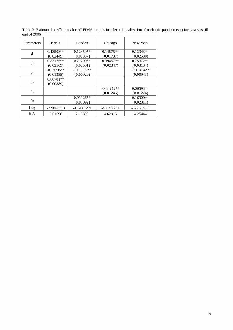
19

Table 3. Estimated coefficients for ARFIMA models in selected localizations (stochastic part in mean) for data sets till end of 2006

Parameters Berlin London Chicago New York

d 0.13508** (0.02449)

0.12450** (0.02337)

0.14575** (0.01737)

0.13343** (0.02530)

p1 0.83175** (0.02569)

0.71290** (0.02501)

0.39457** (0.02347)

0.75372** (0.03134)

p2 -0.19705** (0.01355)

-0.05657** (0.00929)

-0.13494** (0.00943)

p3 0.06701** (0.00889)

q1 -0.34212** (0.01245)

0.06593** (0.01276)

q2 0.03126** (0.01092)

0.16300** (0.02311)

Log -22044.773 -19206.799 -40548.234 -37263.936 BIC 2.51698 2.19308 4.62915 4.25444

20

Table 4. Estimated coefficients for TV-ARFIMA models in selected localizations (stochastic part in mean) for data sets till end of 2006

Parameters Berlin London Chicago New York

d1 0.22125** (0.06226)

0.22433** (0.04195)

0.23569** (0.03090)

0.20983** (0.02534)

d2 0.18573** (0.06150)

0.20675** (0.03762)

0.16581** (0.02755)

0.13720** (0.02392)

d3 0.12426* (0.05419)

0.12139** (0.03806)

0.15370** (0.03012)

0.08730** (0.02805)

d4 0.11300

(0.07879) 0.09526* (0.04489)

0.07751* (0.03779)

0.02371** (0.00570)

d5 0.09314

(0.07551) 0.15367** (0.04636)

0.11551** (0.04494)

0.09307** (0.02746)

d6 0.05721

(0.07933) 0.11829** (0.04575)

0.08134* (0.03510)

0.07291** (0.02840)

d7 0.08325

(0.06652) 0.11144** (0.03757)

0.08632** (0.02101)

0.09397** (0.01648)

d8 0.05313

(0.07046) 0.11001** (0.04321)

0.12838** (0.03417)

0.13001** (0.03120)

d9 0.02210

(0.04923) 0.03107

(0.03307) 0.07211** (0.02981)

0.11684** (0.02535)

d10 0.06670

(0.07000) 0.10506** (0.03575)

0.10624** (0.03149)

0.13682** (0.02332)

d11 0.10518

(0.06974) 0.12539** (0.04729)

0.09641** (0.03984)

0.13892** (0.02817)

d12 0.22694** (0.06801)

0.23048** (0.04721)

0.20587** (0.02960)

0.18336** (0.02564)

p1 0.84426** (0.06499)

0.69713** (0.03644)

0.39474** (0.03133)

0.79849** (0.03038)

p2 -0.20521** (0.02811)

-0.05678** (0.01598)

-0.14922** (0.01449)

p3 0.06813** (0.01631)

q1

-0.34627** (0.01284)

0.10251** (0.02122)

q2 0.03095

(0.02193) 0.18126** (0.01705)

Log -21982.293 -19161.089 -40503.993 -37223.679 BIC 2.51111 2.18904 4.62536 4.25110

21

Table 5. Estimated coefficients for TV-ARMA models in selected localizations (stochastic part in mean) for data sets till end of 2006

Parameters Berlin London Chicago New York

p1 0.87514** (0.01355)

0.84518** (0.01440)

0.65705** (0.01979)

0.65735** (0.02418)

p2 0.86453** (0.01417)

0.84387** (0.01429)

0.59406** (0.02257)

0.59163** (0.02859)

p3 0.81934** (0.01451)

0.78162** (0.01567)

0.60096** (0.02242)

0.54946** (0.03062)

p4 0.79821** (0.01717)

0.77019** (0.01688)

0.48009** (0.02597)

0.46153** (0.03421)

p5 0.78679** (0.01606)

0.79376** (0.01726)

0.53435** (0.02279)

0.52332** (0.03115)

p6 0.77654** (0.01650)

0.78231** (0.01859)

0.50959** (0.02258)

0.53775** (0.02772)

p7 0.77987** (0.01569)

0.77374** (0.01774)

0.48454** (0.02288)

0.53214** (0.03099)

p8 0.76581** (0.01890)

0.77985** (0.01773)

0.55673** (0.02260)

0.57618** (0.02742)

p9 0.74271** (0.01767)

0.69979** (0.01833)

0.49740** (0.02489)

0.57899** (0.02682)

p10 0.78737** (0.01578)

0.77360** (0.01656)

0.51751** (0.02305)

0.58399** (0.02618)

p11 0.79638** (0.01613)

0.77347** (0.01740)

0.52152** (0.02352)

0.57217** (0.02670)

p12 0.85500** (0.01501)

0.81872** (0.01566)

0.62819** (0.02203)

0.63233** (0.02510)

q1

-0.32789** (0.01166)

-0.25001** (0.02194)

q2 0.08885** (0.00896)

0.08098** (0.01526)

Log -22331.654 -19226.689 -40536.765 -37258.832 BIC 2.51790 2.19631 4.62904 4.25489

22

Table 6. Ljung Box test for residual correlations (residuals of ARFIMA, TV-ARFIMA and TV-ARMA models) for data set till end of 2006

Location Model type Statistic Lags

1 2 3 4 5 10 20 50 100

Berlin

ARFIMA Ljung-Box 0.00 0.02 0.08 1.16 1.31 8.83 16.95 36.09 94.67 p- value 0.99 0.99 0.99 0.88 0.93 0.55 0.66 0.93 0.63

TVARMA Ljung-Box 0.01 0.02 0.28 4.35 5.17 21.64 35.18 60.56 126.24 p- value 0.93 0.99 0.96 0.36 0.40 0.02 0.02 0.15 0.04

TVARFIMA Ljung-Box 0.00 0.03 0.16 1.28 1.67 7.84 16.31 36.92 96.29 p- value 0.98 0.98 0.98 0.86 0.89 0.64 0.70 0.92 0.59

London

ARFIMA Ljung-Box 0.00 0.00 2.12 2.91 4.44 9.35 21.63 59.04 96.51 p- value 0.98 1.00 0.55 0.57 0.49 0.50 0.36 0.18 0.58

TVARMA Ljung-Box 0.00 0.10 6.27 6.94 9.62 28.83 42.74 84.81 130.01 p- value 0.95 0.95 0.10 0.14 0.09 0.00 0.00 0.00 0.02

TVARFIMA Ljung-Box 0.00 0.00 1.87 2.59 3.73 7.61 20.96 58.74 98.16 p- value 0.99 1.00 0.60 0.63 0.59 0.67 0.40 0.19 0.53

Chicago

ARFIMA Ljung-Box 0.05 0.12 2.06 3.94 4.90 7.45 15.11 38.16 108.95 p- value 0.83 0.94 0.56 0.41 0.43 0.68 0.77 0.89 0.25

TVARMA Ljung-Box 0.85 5.71 12.23 21.89 32.21 53.15 82.00 108.83 181.03 p- value 0.36 0.06 0.01 0.00 0.00 0.00 0.00 0.00 0.00

TVARFIMA Ljung-Box 0.04 0.10 1.86 3.17 3.94 6.83 14.57 36.31 106.92 p- value 0.84 0.95 0.60 0.53 0.56 0.74 0.80 0.93 0.30

New York

ARFIMA Ljung-Box 0.00 0.00 0.01 0.01 0.74 2.01 9.41 43.29 105.42 p- value 0.99 1.00 1.00 1.00 0.98 1.00 0.98 0.74 0.34

TVARMA Ljung-Box 444.5 2325.5 2387.5 2520.5 2540.7 2553.1 2562.0 2605.3 2705.3 p- value 0.00 0.00 0.00 0.00 0.00 0.00 0.00 0.00 0.00

TVARFIMA Ljung-Box 0.00 0.00 0.02 0.06 0.62 1.41 9.59 42.05 105.48 p- value 1.00 1.00 1.00 1.00 0.99 1.00 0.97 0.78 0.33

23

Table 7. Estimated coefficients for variance models in selected localizations (deterministic part in variance on residuals from ARFIMA) for data set till end of 2006

Parameters Berlin London Chicago New York

0.21065** (0.01847)

2.31744** (0.04034)

1.87803** (0.01981)

-0.00021** (0.00007

-1.43E-05** (3.94E-06)

5.3E-08** (1.53E-08)

-4.58E-12** (1.31E-12)

1.26E-16** (3.73E-17)

0.10795** (0.02441)

0.43793** (0.02778)

0.42624** (0.02806)

0.10214** (0.02663)

0.05366* (0.02451)

0.06899** (0.02723)

-0.05689* (0.02658)

0.08593** (0.02479)

0.20204** (0.02886)

0.18680** (0.02786)

-0.09238** (0.02523)

-0.07879** (0.02420)

-0.16781** (0.02855)

-0.11513** (0.02885)

0.10259** (0.02912)

0.10104** (0.02810)

R2-adjusted 0.00250 0.00269 0.00265 0.02239

0~α

1~α

2~α

3~α

4~α

1~δ

2~δ

3~δ

5~δ

1~γ

2~γ

3~γ

24

Table 8. Estimated coefficients for variance models in selected localizations (deterministic part in variance on residuals on TV-ARFIMA) for data set till end of 2006

Parameters Berlin London Chicago New York

0.22242** (0.01802)

2.31663** (0.03966)

1.87491** (0.01987)

-0.00023** (0.00006)

-1.35E-05** (3.85E-06)

5.87E-08** (1.47E-08)

-4.98E-12** (1.27E-12)

1.36E-16** (3.65E-17)

0.08606** (0.02436)

0.42550** (0.02804)

0.41288** (0.02843)

0.10719** (0.02557)

0.07100** (0.02738)

-0.05489* (0.02652)

0.07787** (0.02462)

0.18288** (0.02845)

0.19831** (0.02763)

-0.09570** (0.02509)

-0.08909** (0.02406)

-0.17524** (0.02843)

-0.12364** (0.02857)

0.10131** (0.02870)

0.09957** (0.02779)

R2-adjusted 0.00258 0.00237 0.00251 0.02248

0~α

1~α

2~α

3~α

4~α

1~δ

2~δ

3~δ

5~δ

1~γ

2~γ

3~γ

25

Table 9. Estimated coefficients for FIGARCH (1,d,1) models in selected localizations (stochastic part in variance for data set till end of 2006

Localization

Based on residuals

from model

Log likelihood

Berlin

ARFIMA

2.12035** (0.16964)

0.01932* (0.01042)

0.07242** (0.01095)

0.00380 (0.0280)

20089.16

London 2.41659** (0.14384)

0.06620** (0.00765)

0.04181** (0.00850)

0.05901** (0.01613)

19754.23

Chicago 1.21720** (0.17352)

0.34901** (0.04983)

0.11634** (0.01551)

0.25609** (0.04562)

20732.99

New York 1.92727** (0.19281)

0.13962** (0.02612)

0.06890** (0.01105)

0.13497** (0.01500)

20263.32

Berlin

TV ARFIMA

2.15941** (0.13916)

0.04721** (0.00222)

0.06326** (0.00987)

0.03394** (0.01162)

19933.94

London 2.44955** (0.13387)

0.01744** (0.00453)

0.04829** (0.00734)

0.0000 (0.00327)

19770.97

Chicago 1.25498** (0.17623)

0.31965** (0.06165)

0.11633** (0.01524)

0.22510** (0.06051)

20643.02

New York 2.18998** (0.12402)

0.01885** (0.00513)

0.06814** (0.00750)

0.01151** (0.00221)

20169.47

in the brackets are standard errors. * coefficient significant on level 5% ** coefficient significant on level 1% Table 10. Results of testing ARFIMA and TVARFIMA models in respect of mean value of forecasting temperature index for January 2007 (out of sample) for selected localizations using evaluation proposed by Caballero et al (2002). Parameter Berlin New York London Chicago Mean in sample 568.38 1043.76 432.34 1355.56 Mean from Arfima-Figarch 566.56* 1040.38* 437.39* 1347.18* Mean from TV Arfima-Figarch 566.42* 1039.95* 437.78* 1345.20* Difference in mean - Arfima-Figarch 1.82 3.38 -5.05 8.39 Difference in mean - TV Arfima-Figarch 1.96 3.80 -5.44 10.36

Quantiles for difference in mean from sample and selected model Arfima-Figarch ( level 95%) 14.31 35.57 16.02 59.61 Arfima-Figarch ( level 99%) 18.89 49.23 19.80 73.77 TV Arfima-Figarch ( level 95%) 18.74 44.01 20.60 79.31 TV Arfima-Figarch ( level 99%) 25.43 59.25 24.97 95.49 * no reasons to reject model on confidence level 1% values of parameters marked with bold font are closer to values from sample Table 11. Results of testing ARFIMA and TVARFIMA models in respect of variance value of forecasting temperature index for January 2007 (out of sample) for selected localizations using evaluation proposed by Caballero et al (2002). Parameter Berlin New York London Chicago Variance in sample 8727.47 18822.45 2879.69 31079.59 Variance from Arfima-Figarch 5478.31 16143.66* 2265.10 41721.51* Variance from TV Arfima-Figarch 9993.03* 26731.31* 4090.33* 74098.22* Difference in variance - Arfima-Figarch -3249.16 -2678.79 -614.58 10641.91 Difference in variance - TV Arfima-Figarch 1265.57 7908.86 1210.65 43018.62

Quantiles for difference in variance from sample and selected model Arfima-Figarch ( level 95%) -1472.40 7666.92 153.59 26593.80 Arfima-Figarch ( level 99%) -626.92 8888.51 443.38 28763.65 TV Arfima-Figarch ( level 95%) 4504.27 18588.23 2474.14 69424.89 TV Arfima-Figarch ( level 99%) 5931.32 23609.88 3053.71 76337.23 * no reasons to reject model on confidence level 1% values of parameters marked with bold font are closer to values from sample

ω β λ ϕ

26

Table 12. Results of testing ARFIMA and TVARFIMA models in respect of mean value of forecasting temperature index for June 2007 (out of sample) for selected localizations using evaluation proposed by Caballero et al (2002). Parameter Berlin New York London Chicago Mean in sample 503.42 191.89 461.90 137.90 Mean from Arfima-Figarch 513.46* 198.64* 458.08* 164.12* Mean from TV Arfima-Figarch 513.07* 195.43* 457.88* 153.32* Difference in mean - Arfima-Figarch 10.04 6.74 -3.82 26.22 Difference in mean - TV Arfima-Figarch -0.39 -3.20 -0.21 -10.80

Quantiles for difference in mean from sample and selected model Arfima-Figarch ( level 95%) 25.59 22.22 5.56 49.75 Arfima-Figarch ( level 99%) 30.84 28.45 10.19 57.47 TV Arfima-Figarch ( level 95%) 20.98 16.86 5.11 33.62 TV Arfima-Figarch ( level 99%) 24.67 21.64 8.64 38.81 * no reasons to reject model on confidence level 1% values of parameters marked with bold font are closer to values from sample Table 13. Results of testing ARFIMA and TVARFIMA models in respect of variance value of forecasting temperature index for June 2007 (out of sample) for selected localizations using evaluation proposed by Caballero et al (2002). Parameter Berlin New York London Chicago Variance in sample 1627.37 2254.39 1361.38 2655.18 Variance from Arfima-Figarch 5701.59* 4843.34* 1909.45* 7402.68* Variance from TV Arfima-Figarch 3386.89* 3350.12* 1715.08* 4677.11* Difference in variance - Arfima-Figarch 4074.23 2588.95 548.06 4747.50 Difference in variance - TV Arfima-Figarch 1759.53 1095.74 353.69 2021.94

Quantiles for difference in variance from sample and selected model Arfima-Figarch ( level 95%) 6244.20 4665.19 1201.85 8163.11 Arfima-Figarch ( level 99%) 6986.78 5155.21 1435.65 9087.77 TV Arfima-Figarch ( level 95%) 3110.50 2500.58 922.75 3957.29 TV Arfima-Figarch ( level 99%) 3608.11 2856.59 1185.16 4505.12 * no reasons to reject model on confidence level 1% values of parameters marked with bold font are closer to values from sample Table 14. Final prices for January 2007 put options received using ARFIMA-FIGARCH and TVARFIMA-FIGARCH models for selected localizations. Model type used in pricing process Berlin London Chicago New York Arfima-Figarch £698.63 £449.67 $1,911.35 $1,185.35TV Arfima-Figarch £943.94 £602.74 $2,552.18 $1,526.48Difference in relation to ARFIMA-FIGARCH [%] 35.11% 33.94% 33.53% 28.78% Table 15. Final prices for June 2007 put options received using ARFIMA-FIGARCH and TVARFIMA-FIGARCH models for selected localizations. Model type used in pricing process Berlin London Chicago New York Arfima-Figarch £708.80 £412.69 $785.54 $646.29TV Arfima-Figarch £548.16 £391.31 $627.43 $538.59Difference in relation to ARFIMA-FIGARCH [%] -22.66% -5.18% -20.13% -16.66%