Very fast simulation of nonlinear ... -...

By Allan P. Engsig-Karup, Morten Gorm Madsen and Stefan L. Glimberg

DTU Informatics

Workshop on “GPU computing today and tomorrow”

Kgs. Lyngby, DTU, Aug 18, 2011.

Very fast simulation of nonlinear water waves in very large numerical wave tanks on

affordable graphics cards

Shoaling on a semi-circular bar (Exp. by Whalin, 1971)

(Technical University of Denmark) 13 / 22

Requirements

General requirementsv Ability to estimate or predict wave kinematics and wave loads on structuresv Estimation of influence of sea floor on wave transformationsv Accurate representation of wave propagation over long distances and timesv Numerical basis for a tool should be generally applicable and reliable(v) Possibility to simulate waves in realistic structural settings

Current research directionsv Development of an efficient and scalable parallel algorithm for the numerical toolv Utilize many-core hardware to maximize performance for fast analysis and large problem sizes- New robust numerical engineering tools for wave-structure interaction (floating wave-energy devices, windmill foundations, etc.)

Motivation

Development of a new efficient numerical tool for wave-structureinteraction for large-scale nonlinear wave problemsMultiple applications

Wave loadings on ships, offshore, platformsInfluence of the bottom interaction in coastal regionsSeakeeping & manouevring...

Potential flow theory can account for a very broad range of wavephenomena in offshore and coastal regions

Viscous effects neglectedFlow is irrotationalNonbreaking waves


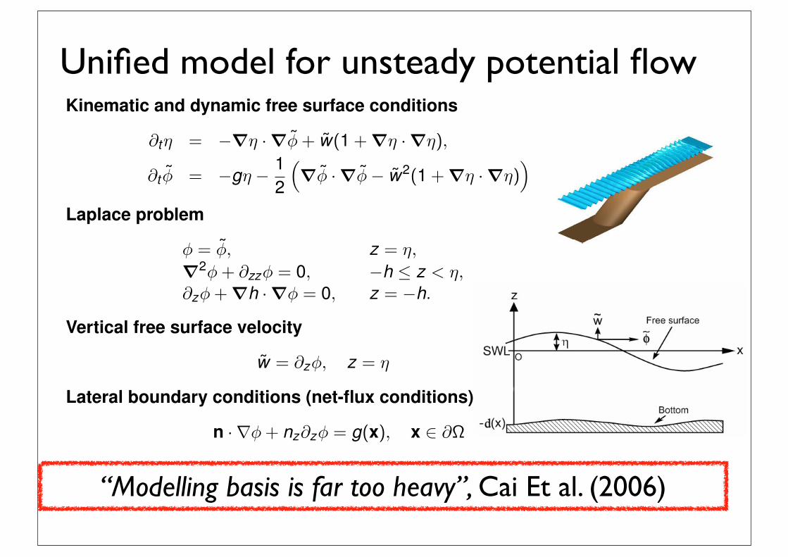
Unified model for unsteady potential flowPotential flow formulationKinematic and dynamic free surface conditions

∂tη = −∇η · ∇φ + w(1 + ∇η · ∇η),

∂t φ = −gη − 12

∇φ · ∇φ− w2(1 + ∇η · ∇η)

Laplace problem

φ = φ, z = η,∇2φ + ∂zzφ = 0, −h ≤ z < η,∂zφ + ∇h · ∇φ = 0, z = −h.

Vertical free surface velocity

w = ∂zφ, z = η

Lateral boundary conditions (net-flux conditions)

n ·∇φ + nz∂zφ = g(x), x ∈ ∂Ω


Notation sketch for numerical wave model

Free surface a priori unknown.Nonlinear kinematic and dynamic constraints at free surface.Kinematic constraint at sea bottom.Laplace problem in the interior.Lateral boundary conditions have to be specified.




“Modelling basis is far too heavy”, Cai Et al. (2006)

OceanWave3D- a wave model for coastal engineering

Case study• Can we use the new GPU technology and programming

models to leverage performance over existing CPU applications?

• Proof-of-concept case study

• Develop new massively parallel algorithm for an engineering application that can utilize GPU architectures

• Enable fast engineering analysis of fully nonlinear waves at large scales by implementation on affordable commodity hardware

• Find out how fast can we do robust (real-time?) computer-based analysis and experiments with OceanWave3D model

“Modelling basis is far too heavy”, Cai Et al. (2006)

OceanWave3D

Can we do better?

Courtesy of The Hydraulics and Maritime Research Centre (HMRC) at University College Cork

Numerical methodAn accurate and robust arbitrary-order finite difference method.

Computational bottleneck problem (Laplace)Efficient and scalable iterative solution of large sparse linear system every time step.

=> Entire algorithm is explicit.=> Algorithmic efficiency for both linear and nonlinear simulations established.

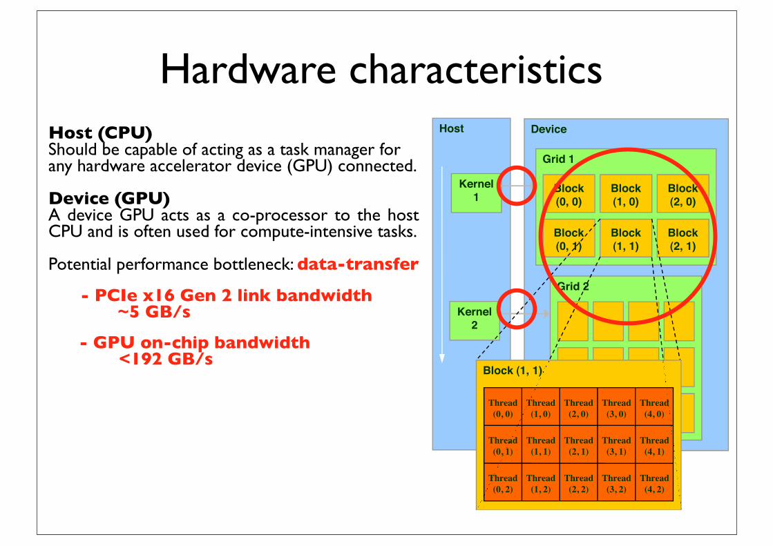
Hardware characteristicsHost (CPU)Should be capable of acting as a task manager for any hardware accelerator device (GPU) connected.

Device (GPU)A device GPU acts as a co-processor to the host CPU and is often used for compute-intensive tasks.

Potential performance bottleneck: data-transfer

!"#$%&'()*+,+'-(.'/+0'(1203+&'0&%2'(45'0%&+"*(6"-'7

! "#$%&'()*+,,)(,-*./-'()*+,,-)/+-)(-0)(+-1$)*2,-*)/*#((+/%$3

! 4.*5-.*%&6+-1$)*2-&,-,'$&%-&/%)-7.(',-89:-%5(+.;,<-./;-%5(+.;,-7&%5&/-.-7.('-.(+-+=+*#%+;-'53,&*.$$3-&/-'.(.$$+$-8>-*3*$+,<

Host

Kernel 1

Kernel

Device

Grid 1

Block(0, 0)

Block(1, 0)

Block(2, 0)

Block(0, 1)

Block(1, 1)

Block(2, 1)

Grid 2

Meeting on Parallel Routine Optimization and Applications – May 26-27, 2008 25

! ?+@&,%+(,-./;-AB"-.(+-,'$&%-.0)/@-.*%&6+-%5(+.;,-C()0-.*%&6+-1$)*2,

! ".=&0#0-/#01+(-)C-.*%&6+-1$)*2,-;+'+/;,-)/-5)7-0./3-(+@&,%+(,-./;-AB"-%5+-2+(/+$-(+D#&(+,

! B&@5-'.(.$$+$&,0-&,-*(#*&.$-%)-5&;+-0+0)(3-$.%+/*3-13-)6+($.''&/@-0+0)(3-.**+,,+,-7&%5-*)0'#%.%&)/

Kernel 2

Block (1, 1)

Thread(0, 1)

Thread(1, 1)

Thread(2, 1)

Thread(3, 1)

Thread(4, 1)

Thread(0, 2)

Thread(1, 2)

Thread(2, 2)

Thread(3, 2)

Thread(4, 2)

Thread(0, 0)

Thread(1, 0)

Thread(2, 0)

Thread(3, 0)

Thread(4, 0)

- PCIe x16 Gen 2 link bandwidth~5 GB/s

- GPU on-chip bandwidth <192 GB/s

Iterative methods Iterative methods vs. direct methods?low-storage requirements straightforward

with iterative method for the systemSummary of development and analysis of past work on the efficient solution of the model equations

Contributions 2D 3D Iterative method Accuracy Storage

Li & Fleming (1997) Multigrid (MG) 2nd Low

Bingham & Zhang (2006) GMRES+LU Flexible High

Engsig-Karup, Bingham & Lindberg (2008)

GMRES+MG Flexible High

Engsig-Karup (2010)Defect Correction

+ LU/MGFlexible Low

- Multigrid method is O(n), robust, fast convergence for 2nd order, is memory-limited- The Standard GMRES method has increasing workload per iteration, not memory-limited- DC method, is memory-limited and requires less global synchronization- DC and GMRES methods, robust and require efficient preconditioning to be fast

Defect Correction method

Sparse matrix-vector product (matrix-free and minimal storage)

Preconditioning problem - solve cheaply and efficiently

Error estimator (gather step)

Stop criteria (efficiency)

since ![k!1] ! e[k!1]. This suggests that it is possible to control the error (implyingindirectly controlling the iteration count) by an absolute error condition of the form

"![k!1]" # atol (31)

giving the user control to decide the acceptable level of absolute accuracy in the finalresult of the iterative procedure. Importantly, the magnitude of the corrections ![k],k = 0, 1, ..., can be computed at low computational cost in some appropriate norm.Furthermore, this condition can be used to guarantee that the iteration procedure canbe stopped once the first log10(atol) significant digits remain unchanged in the sequenceof iterates if we use the l"-norm.

In some cases, we rather want to reduce the error relative to the initial error computedbased on the initial guess, and this can be taken into account in (31) by defining a mixederror condition of the form

"![k!1]" # rtol · "![0]" + atol (32)

Remark, that a condition of the form (31) is straightforward to use in other iterativemethods when the preconditioner M is used in left-preconditining and is a good precon-ditioner for A, i.e M ! A, since

![k] = $M!1(b $A![k]) (33)

will then be an estimate of the error due to (14). In other words, (33) can be interpreted asthe residual of the left-preconditioned linear system of equations. This stopping criteriawas employed in the earlier work [13] which is the default stopping criteria implementedfor the GMRES routine included in the software library package SPARSKIT that wasused.

3.4. AlgorithmA generic algorithm for the DC method for solving a system of equations Ax = b

can be defined by the pseudocode defining Algorithm 1, where M ! A represents themapping of an approximate coe"cient matrix for the problem, and which is typicallya low-order accurate approximation. A convergence criterion needs to be defined for(line 5) the algorithm (e.g. (32) as discussed in section 3.3). The algorithm is referredto as a defect correction method when A represents the full time-dependent coe"cientmatrix of (7) and M ! Ap a corresponding inexact approximation to A, e.g. a p’th ordertime-constant matrix for the linearized Laplace problem (4). Implemented Matlab andFortran versions of the algorithm are available for download from the author’s webpage.

Algorithm 1: Defect Correction Method for solution of Ax = b

Choose x[0] /* initial guess */1

k = 02

repeat3

r[k] = b $Ax[k] /* high-order defect */4

Solve M![k] = $r[k] /* preconditioning problem */5

x[k+1] = x[k] $ ![k] /* defect correction */6

k = k + 17

until no convergence and k < maximum iterations ;8

12

Good initial guess (last solve)

- Algorithm suitable for mixed precision calculations- Two-step recurrence basis for minimal memory footprint

Peer Review Only

6

problem (2). Thus, the computational bottleneck problem is the solution of the linear system (9)every time step of the time-integration of the evolution of the free surface problem. This linearsystem can be solved efficiently starting from some initial guess![0] by a DCmethod with iterationsgiven in compact form

![k+1] = !

[k] + ![k], ![k] = M!1(b !A![k]), k = 0, 1, 2, ... (10)

where M " A can conceptually be considered as (the action of) a preconditioning matrixresponsible for minimizing de-acceleration of convergence over the single-iteration schemeachieved if M # A. When a full high-order discretization is employed for the discretization of(9) and a reduced-order multigrid method is employed for determining the correction ![k] in thepreconditioning step in (10), the resulting method can be perceived as a p-multigrid method and isgiven in pseudocode in Algorithm 1.In this work, we employ a second-order multigrid discretization preconditioning strategy based

on a time-constant discretization of the linearized system matrix (assume " " 0 in (10)) whichwas demonstrated to be efficient by Engsig-Karup (2010). With the resulting DC method basedon a two-step recurrence combined with the same multigrid preconditioning strategy proposed byEngsig-Karup et al. (2009), the storage requirements can be kept minimal (see also discussionin Section 5.4). The best preconditioning strategy was found to be a multigrid method basedon a Red-Black Zebra-Line Gauss-Seidel (RB-ZL-GS) smoothing strategy combined with semi-coarsening. The multigrid strategy MG-RB-ZL-GS-1V(1,1) based on a V-cycle with one pre- andpost-smoothing was found to be efficient for the entire application range from shallow to deepwater in the current numerical model. This is in contrast to point-based smoothing methods whichexhibit slow convergence when discrete anisotropy is high (fx. in shallow water). We therefore onlyconsider this strategy in the following.

Algorithm 1: Defect Correction Method for approximate solution of A! = b

Choose ![0] /* initial guess */1k = 02repeat3

r[k] = b !A![k] /* high-order defect */4SolveM![k] = r[k] /* preconditioning problem */5![k+1] = ![k] + ![k] /* defect correction */6k = k + 17

until (||r[k]|| < ||r[0]||·rtol+atol) and (k < maxiter) ;8

Geometric multigrid methods are multi-level methods (see Trottenberg et al. (2001)) and can beconstructed from three basic components, namely, a fine-to-coarse grid (restriction) operator, acoarse-to-fine (prolongation) operator and a smoothing (relaxation) operator. With second-orderdiscretizations employed, it is sufficient to use tri-linear interpolation for the adjoint grid-transferoperations. The remaining essential component is the smoother.For each of the Nx · Ny the free surface grid points, the RB-ZL-GS smoothing strategy requires

solving a small m $ m linear system of equations (with m = Nz). We employ a discretization ofthe transformed Laplace problem with a single layer of fictitious ghost points below the bottom forimposing kinematic boundary conditions. Then these small linear systems have a general and nearlytri-diagonal structure of the form

!

"

"

"

"

"

#

b1 c1 0a2 b2 c2

. . . . . . . . .am!1 bm!1 cm!1

0 em am bm

$

%

%

%

%

%

&

!

"

"

"

"

"

#

x1

x2

x3...

xm

$

%

%

%

%

%

&

=

!

"

"

"

"

"

#

d1

d2

d3...

dm

$

%

%

%

%

%

&

(11)

This system can be solved directly using a modified Thomas Algorithm (TA) which takes intoaccount an extra nonzero coefficient denoted em. This changes the standard Thomas algorithm to a

Copyright c! 2010 John Wiley & Sons, Ltd. Int. J. Numer. Meth. Fluids (2010)Prepared using fldauth.cls DOI: 10.1002/fld

Page 6 of 17

http://mc.manuscriptcentral.com/fluids

International Journal for Numerical Methods in Fluids

123456789101112131415161718192021222324252627282930313233343536373839404142434445464748495051525354555657585960

OceanWave3D Scalability

10

memory. The shared interleaved memory provides fast low-latency access when threads in activewarps all access either the same or different memory banks. If this is not the case, the memoryrequests are serialized and performance may degrade. On the GPUs the local memory spaces toeach stream processor is a scarce resource and are shared among threads within active thread blocksscheduled for execution. Therefore, it is important to first optimize the implemented kernels to takeadvantage of the memory hierarchy. Then, good kernel execution configurations should be foundthat balance the resource available for each thread and at the same time ensure that the streamingprocessors can be fully occupied with computations.To minimize data-transfer between host and device, we employ a strategy where initial data and

finite difference stencil weights are initially pre-processed on the host and then transferred to thedevice for subsequent reuse.The data needed to solve this three-dimensional Laplace problem (3) is the two-dimensional free

surface quantities !(x, y, t) and "(x, y, t) for a given state together with the still-water depth h(x, y).The required storage is minimal compared to that of the iterative solver (10). Furthermore, byemploying a #-transformation (3) between the physical grid to a regular unity-spaced computationalgrid (see (26)), the amount of data storage for the finite difference coefficients of all stencils to beused frequently in the iterative part of the solution process can be stored in the low-latency cachedconstant memory. This makes it possible to reduce storage requirements for the minimal set ofstencils coefficients to a small array that easily fit within the 64 KB limit of the constant memory.For the preconditioned iterative DC method (10), we need to store two fine grid arrays for the

iterates together with intermediate results on the coarser grids for the multigrid preconditioning.The total storage requirement for the coarse grid levels in multigrid is bounded independently ofthe number of grid levels chosen by

!

!

k=0nsk =

"

ss"1

#

n, with s a reduction factor indicatinghow aggressively the coarsening strategy is in terms of reducing the grid points for each gridlevel. For example, with a coarsening strategy based on simultaneous halving of grid point in thehorizontal directions (s = 4) only between grid levels, at most 4

3n elements are needed for datastorage. Dependent on the spatial resolution employed, typically, semi-coarsening is employed inthe horizontal plane until the grid increments are of similar size. Thereafter, standard coarsening isemployed (s = 8).Results from memory scaling tests are presented in figure 1 which shows the total amount of

global device memory used as a function of problem size. The test demonstrates linear scaling inboth single and double precision implementations. Furthermore, it is clear that with 4GB RAMmemory it is possible to solve a Laplace problem of size up to close to 50/100 million degrees offreedom in single/double precision. This makes it possible to solve a system which is approximately19 times larger than the large-scale validation test presented by (8) for propagating stream functionwaves with 4 GB RAM available.

Memory[MB]

Problem size [grid points]

doublesingleO(n)

103 104 105 106 107 108 10910"2

10"1

100

101

102

103

104

Figure 1. Scalability test of measured memory footprint for both single and double precision storage.


8 G. DUCROZET ET AL.

103

104

105

106

10710

0

101

102

103

104

103

104

105

106

10710

-3

10-2

10-1

100

101

DC+MGDC+MGO(N)-scalingO(N)-scaling

NN

Mem

ory[M

B]

CPU/iter[s]

Figure 1. Scaling RAM memory use and computational effort - 3D simulation - 6th order

It appears from this figure that the memory requirement evolves linearly with the number of

points in the domain. At the same time, the computational effort scales also perfectly linearly

(even for quite large number of points in the domain: here up to 2.4 106 points). This study is

made on 3D configuration since OceanWave3D model has been especially designed for this and

that this is the most demanding test-case (to achieve this linear scaling). This is the multigrid

preconditionning strategy which allows to retain the linear scaling of both computational effort and

memory requirement (see Engsig-Karup et al. [4]). Note that these linear scalings are also obtained

for 2D computations.

3.2. HOS

Figure 2 presents the same plots than in previous paragraph with the scaling of RAM memory use

(left part) and computational effort per Runge-Kutta step (right part) with respect to the number

of points (Nx Ny)for the HOS method. This figure was obtained for a typical 3D simulation

with a HOS order fixed to M = 5. Then, this figure is slightly different than the one obtained

for OceanWave3D (for computational effort). Furthermore, notice that the HOS model takes full

Copyright c! 0000 John Wiley & Sons, Ltd. Int. J. Numer. Meth. Fluids (0000)

Prepared using fldauth.cls DOI: 10.1002/fld

Implementation choices matters- Mapping to GPU resulted in a reduction of more than x10 in memory footprint- from 5.000.000 up to 50.000.000 degrees of freedom in Laplace problem (double precision)- Less than 4GB RAM required

CPU GPU

Throughput performance

13

6.3. Benchmarking

We benchmark the complete algorithm described in Sections 3 and 4 implemented for heterogenousCPU-GPU hardware. For benchmarking we employ spatial discretizations of order 2, 4 and 6for defect corrections and employ a second-order time-constant MG-RB-ZL-GS-1V(1,1) multigridpreconditioning strategy in each case. For practical computations, it is advantageous to balance thediscretization parameters with the accuracy needs to best utilize the available resources.For the performance test we solve for the propagation of unsteady nonlinear periodic stream

function solutions (see (24)) at shallow depth (parameters for dispersion are kh = 0.5 andnonlinearity H/L = 30%(H/L)max). To measure overall throughput performance, the choice oftest case is not important as long it is numerically stable during tests.

Time/Iter[s]

n103 104 105 106 107 10810!3

10!2

10!1

100

101

(a) Absolute timings.n

Speedup

103 104 105 106 107 1080

10

20

30

40

50

(b) Speedup relative to CPU (single thread) code in doubleprecision arithmetic.

Figure 2. Scalability tests and performance comparisons in double precision arithmetic for Quadro FX 5800(! •!), GeForce GTX 480 (!!!), C2050 with ECC (!"!) and C2050 without ECC (!#!) versus CPU(single thread) code (!$!). Sixth order spatial discretization employed. Same algorithm for iterative solver

DC+MG-ZLGS-V(1,1) has been employed on each architecture.

In the performance tests we have employed a base configuration (Ny, Nz) = (7, 6). In the x-direction we have used a resolution up to Nx = 671745 points and the wave resolution is kept fixedclose to 32 Points Per Wave (PPW) in any test configuration. The waves propagate along the x-axis.At the largest resolution, it is possible to resolve a total of 20995 wave lengths in the x-direction ofthis NWT. For the time-integration we employ ERK4 with a Courant number Cr = c !t

!x ! 0.5.Scalability tests are presented in figure 2(a). The absolute timings presented are suitable for

comparison with performance of other models. A relative performance comparison with thealgorithm executed on the CPU of test environment 3 is presented in figure 2(b). We find thatthe implemented GPU model outperforms the CPU implementation for all problem sizes wheren > 2 · 104 in each test environment when double precision arithmetic is used. If instead singleprecision arithmetic is used, the throughput performance of one iteration of the iterative solver canbe improved significantly since the data-storage for all variables will be halved. As illustrated infigure 3 the performance for a single precision solver is improved up to 42% with ECC and 52%without ECC compared to a double precision solver with ECC (cf. figure 2(a)). This improvementis achieved for the largest problem sizes only.For the best architecture, namely the C2050 processor with ECC on, we have measured the

relative sensitivity to the discretization order of accuracy as presented in figure 4. These resultsshows that with the second discretization as the reference, the throughput performance is reducedwith up to 25 percent when we use a 6th order discretization instead of a 2nd order discretization.Thus, we conclude that the performance does not change dramatically with changes in thediscretization order. This is attributed to that most kernels in the algorithmic strategy are memorybound and does not experiences any changes in algorithmic intensity when discretization order


103 104 105 106 107 10810 3

10 2

10 1

100

101

Tim

e/Ite

r [s]

n

CPUQuadro FX 5800 (gaming)GeForce GTX 480 (gaming)C2050 w/ECCC2050 wo/ECC

- Throughput performance curves a means for evaluating and confirming performance and capturing current state-of-the-art in practice. - Without these difficult to make fair comparison between different models

Remarks:- Scalable work effort- Good performance across architectures

Engsig-Karup, Allan; Madsen, Morten; Glimberg, Stefan. A massively parallel GPU-accelerated model for analysis of fully nonlinear free surface waves. Journal: International Journal for Numerical Methods in Fluids, 2011.

Relative speedup

13

6.3. Benchmarking

We benchmark the complete algorithm described in Sections 3 and 4 implemented for heterogenousCPU-GPU hardware. For benchmarking we employ spatial discretizations of order 2, 4 and 6for defect corrections and employ a second-order time-constant MG-RB-ZL-GS-1V(1,1) multigridpreconditioning strategy in each case. For practical computations, it is advantageous to balance thediscretization parameters with the accuracy needs to best utilize the available resources.For the performance test we solve for the propagation of unsteady nonlinear periodic stream

function solutions (see (24)) at shallow depth (parameters for dispersion are kh = 0.5 andnonlinearity H/L = 30%(H/L)max). To measure overall throughput performance, the choice oftest case is not important as long it is numerically stable during tests.

Time/Iter[s]

n103 104 105 106 107 10810!3

10!2

10!1

100

101

(a) Absolute timings.n

Speedup

103 104 105 106 107 1080

10

20

30

40

50

(b) Speedup relative to CPU (single thread) code in doubleprecision arithmetic.

Figure 2. Scalability tests and performance comparisons in double precision arithmetic for Quadro FX 5800(! •!), GeForce GTX 480 (!!!), C2050 with ECC (!"!) and C2050 without ECC (!#!) versus CPU(single thread) code (!$!). Sixth order spatial discretization employed. Same algorithm for iterative solver

DC+MG-ZLGS-V(1,1) has been employed on each architecture.

In the performance tests we have employed a base configuration (Ny, Nz) = (7, 6). In the x-direction we have used a resolution up to Nx = 671745 points and the wave resolution is kept fixedclose to 32 Points Per Wave (PPW) in any test configuration. The waves propagate along the x-axis.At the largest resolution, it is possible to resolve a total of 20995 wave lengths in the x-direction ofthis NWT. For the time-integration we employ ERK4 with a Courant number Cr = c !t

!x ! 0.5.Scalability tests are presented in figure 2(a). The absolute timings presented are suitable for

comparison with performance of other models. A relative performance comparison with thealgorithm executed on the CPU of test environment 3 is presented in figure 2(b). We find thatthe implemented GPU model outperforms the CPU implementation for all problem sizes wheren > 2 · 104 in each test environment when double precision arithmetic is used. If instead singleprecision arithmetic is used, the throughput performance of one iteration of the iterative solver canbe improved significantly since the data-storage for all variables will be halved. As illustrated infigure 3 the performance for a single precision solver is improved up to 42% with ECC and 52%without ECC compared to a double precision solver with ECC (cf. figure 2(a)). This improvementis achieved for the largest problem sizes only.For the best architecture, namely the C2050 processor with ECC on, we have measured the

relative sensitivity to the discretization order of accuracy as presented in figure 4. These resultsshows that with the second discretization as the reference, the throughput performance is reducedwith up to 25 percent when we use a 6th order discretization instead of a 2nd order discretization.Thus, we conclude that the performance does not change dramatically with changes in thediscretization order. This is attributed to that most kernels in the algorithmic strategy are memorybound and does not experiences any changes in algorithmic intensity when discretization order


103 104 105 106 107 1080

10

20

30

40

50

n

Spee

dup

rela

tive

to o

ptim

ized

CPU

cod

e

GeForce GTX 480 (gaming)Quadro FX 5800 (gaming)C2050 w/ECCC2050 wo/ECC

- Mapped algorithm to GPU faster than same algorithm on CPU for all problem sizes of interest- Better performance the larger the problem, i.e. speedup where it is needed- Gaming card beats high-end HPC GPU processors!

Engsig-Karup, Allan; Madsen, Morten; Glimberg, Stefan. A massively parallel GPU-accelerated model for analysis of fully nonlinear free surface waves. Journal: International Journal for Numerical Methods in Fluids, 2011.

Precision requirements?

• How much precision do we really need in computations?

• Can we trade precision for speed?

• Is it feasible for practical computations?

Most applications today use double precision maths to minimize accumulation of round-off errors.

If single precision math can be used in parts of code, it is possible to

• Half the size of data-transfers

• For some architectures single precision operations can be processed at more than twice the speed, e.g. GPUs.

Free lunch: x2?

Single precision vs. double precision

0 2 4 6 8 10 12

10 10

10 5

100

Double precision

Iterations

Erro

r

0 5 10 15 20

10 10

10 5

100

Single precision

Iterations

Erro

r

Residual error, rAbsolute error, rTruncation Error, T.E.Rel. Residual errorEst. errorOptimalAlgebraic error

Deep water, SF waves, kh=6.14, H/L=90% , Nx=15, Nz=9, 6th order stencils

- Overall accuracy can be maintained in solution of Laplace problem

Single precision vs. double precision

0 20 40 60 80 10010 6

10 5

10 4

10 3

10 2

10 1

100

t/T

Erro

r

SingleDouble

Parameters: Intermediate water, SF waves, Direct solutionkh=1, H/L=90% , Nx=15, Nz=9, 6th order stencilsSG(6,10) filter strategy every 10 time step

0 20 40 60 80 10010 6

10 5

10 4

10 3

10 2

10 1

100

t/TEr

ror

SingleDouble

Without filtering With filtering

- Errors tends to accumulate faster in single precision without stabilization- Control at the expense of a mild inexpensive filtering strategy

OceanWave3D model14Speedup

n103 104 105 106 107 1080

0.25

0.5

0.75

1

1.25

1.5

Figure 3. Speedup in scalability tests for C2050 withECC for a single versus double precision arithmeticcomparison. Single precision with ECC (!!!) andwithout ECC (!"!). Iterative solver DC+MG-ZLGS-V(1,1) and sixth order spatial discretization

have been employed.

Speedup

n103 104 105 106 107 1080

0.25

0.5

0.75

1

1.25

1.5

Figure 4. Speedup in scalability tests for C2050 withECC in double precision arithmetic. Discretization issecond order (reference, !!!), fourth order (!"!)and sixth order (!#!). Iterative solver DC+MG-

ZLGS-V(1,1) has been employed.

changes. The mapped GPU implementation achieves a speedup up to x40/x49 in double/singleprecision in comparison with the existing efficient and fairly optimized reference CPU (singlethread) Fortran 90 double precision code used by (8; 9). For computations using ERK4 (with a stagecount of four) and average number of iterations between 5-10, we find that the compute time per timestep is between 20-40 times larger than the throughout performance per iteration measured in figure2(a). This implies that for n = 104 one time step is processed in about 0.04 ! 0.08s, for n = 105 ittakes 0.08 ! 0.16s and for n = 106 it takes 0.4 ! 0.8s of compute time. For example, we estimatethat without taking accuracy into account this enable throughput performance improvements ofclose to one order in magnitude reduction in comparison with the benchmarks collected and reportedby (31) for a few known free surface models. The benchmarks provided in this section can be usedto predict general performance based on chosen discretization parameters.

6.4. Performance prediction

For practical purposes it can be useful to use the absolute timings presented in figure 2(a) to predicthow fast we can resolve one wave period of a wave. This can be done with the following simplerelationship

Compute timeWave period "

Compute timeiteration ·

IterationsTime step ·

Time stepsWave period

which can be expressed more mathematically (in terms of standard dimensionless quantities)

tcompute(n)

T"Compute timeiteration · K, K " (SRK · Iavg) ·

PPWCr

(15)

where K is a parameter defined in terms of the average iteration count for the solution of (9) usingthe DC method (10) and SRK is the number of stages in the Runge-Kutta ODE solver employed. Ifwe assume that we can resolve a wave with an accuracy of less than two percent in dispersion (phasespeed) if we use 10 grid points in the vertical and 10 points per wave length (e.g. see the dispersionanalysis by (9)), then we find that K " 4 · 5 · 10

0.5 = 400. Thus, we need to multiply the absolutetimings given in figure 2(a) with 400 to estimate how fast we can resolve the propagation of thesuch waves in a domain of size n over one wave period within two percent accuracy in dispersion.For comparison of performance differences between free surface models, e.g., Boussinesq-type

and fully nonlinear free surface models, it is fair to examine how fast the solution can be advanced


Preliminary tests in SP

Total GPU vs. CPU Speedup=========================C2050 : x57 (measured)GTX 480 : x60 (estimated)For sufficiently large problems

OceanWave3D code for GPUs not considered fully optimized.

Brute-force auto-tuning of most expensive kernels level have been used.

No free lunch yet! Expected a factor x2 when using single over double precision...

Outlook

• Further optimization and auto-tuning of existing implementation could improve efficiency further

• Investigate means for leveraging productivity in code development (development cost is often overlooked and not negligible)

• Replace CUDA with OpenCL for better portability across hardware platforms, e.g. execution utilizing both CPUs and GPUs.

• Enable use of multi-GPU systems to efficiently solve even larger problems.

• Real-time computations and analysis requires fast algorithms, improvements in hardware and implementation/optimization effort.

Linear diffraction of waves semi-circular channel3

3Dalrymple, Kirby & Martin (1994), Appl. Ocean Res. 16.


General-purpose computing

Many different applications from science and engineering show-cased in Nvidia’s CUDA zone. All applications written in the CUDA framework after 2007!

Questions



Linear diffraction of waves semi-circular channel3

3Dalrymple, Kirby & Martin (1994), Appl. Ocean Res. 16.


Flow field by superposition

Figure: Snapshot of linear scattering about a vertical cylinder in the open sea.


!"#$%&'()*+,(#-)$.*/012

3(4$*5$67*(68*(9.7*:;6$.<

=-;65$*)(>$%

3(4$*#(?$%

@0

! A&6$(%*B(8C*/DED2*#;8$)7*

! F;#9&6$8*G(4$*5$6$%(H&;6*(68*(9.;%-H&;6*6$(%*G$.H*G())

!3(4$*(9.;%-H&;6*6$(%*$(.H*I*.;"HJ*G()).&6*9(..&6

! F;#-(%&.;6*G&HJ*(6()>H&'()*.;)"H&;6*9>*B$66>*I*B%&'$*/KLMD2*

Contact infoAllan P. Engsig-KarupE-mail: [email protected] Professor in Scientific ComputingDepartment of Mathematics and ModelingTechnical University of Denmark

Very fast simulation of nonlinear ... -...

Documents

Transcript of Very fast simulation of nonlinear ... -...