Version 4guard Gile Delhi

Version 4.0

Fitting Modelsto Biological Datausing Linear andNonlinearRegression

A practical guide tocurve fitting

Harvey Motulsky &Arthur Christopoulos

Copyright 2003 GraphPad Software, Inc. All rights reserved.

GraphPad Prism and Prism are registered trademarks of GraphPad Software, Inc.GraphPad is a trademark of GraphPad Software, Inc.

Citation: H.J. Motulsky and A Christopoulos, Fitting models to biological data usinglinear and nonlinear regression. A practical guide to curve fitting. 2003, GraphPadSoftware Inc., San Diego CA, www.graphpad.com.

Second printing, with minor corrections.

To contact GraphPad Software, email [email protected] or [email protected].

Contents at a Glance

A. Fitting data with nonlinear regression.................................... 13

B. Fitting data with linear regression .......................................... 47

C. Models ....................................................................................58

D. How nonlinear regression works........................................... 80

E. Confidence intervals of the parameters .................................. 97

F. Comparing models ................................................................ 134

G. How does a treatment change the curve?.............................. 160

H. Fitting radioligand and enzyme kinetics data ....................... 187

I. Fitting dose-response curves .................................................256

J. Fitting curves with GraphPad Prism......................................296

3

Contents

Preface ........................................................................................................12

A. Fitting data with nonlinear regression.................................... 131.

Example data ............................................................................................................................13Step 1: Clarify your goal. Is nonlinear regression the appropriate analysis? .........................14Step 2: Prepare your data and enter it into the program ........................................................ 15Step 3: Choose your model....................................................................................................... 15Step 4: Decide which model parameters to fit and which to constrain..................................16Step 5: Choose a weighting scheme ......................................................................................... 17Step 6: Choose initial values..................................................................................................... 17Step 7: Perform the curve fit and interpret the best-fit parameter values ............................. 17

Avoid Scatchard, Lineweaver-Burk, and similar transforms whose goal is to create a straight line ............................................................................................................................19Transforming X values ............................................................................................................ 20Don’t smooth your data........................................................................................................... 20Transforming Y values..............................................................................................................21Change units to avoid tiny or huge values .............................................................................. 22Normalizing ............................................................................................................................. 22Averaging replicates ................................................................................................................ 23Consider removing outliers ..................................................................................................... 23

Choose a model for how Y varies with X................................................................................. 25Fix parameters to a constant value? ....................................................................................... 25Initial values..............................................................................................................................27Weighting..................................................................................................................................27Other choices ........................................................................................................................... 28

Does the curve go near your data? .......................................................................................... 29Are the best-fit parameter values plausible? .......................................................................... 29How precise are the best-fit parameter values? ..................................................................... 29Would another model be more appropriate? ......................................................................... 30Have you violated any of the assumptions of nonlinear regression? .................................... 30

Confidence and prediction bands ........................................................................................... 32Correlation matrix ................................................................................................................... 33Sum-of-squares........................................................................................................................ 33R2 (coefficient of determination) ............................................................................................ 34Does the curve systematically deviate from the data? ........................................................... 35Could the fit be a local minimum? ...........................................................................................37

Poorly defined parameters ...................................................................................................... 38Model too complicated ............................................................................................................ 39

An example of nonlinear regression ......................................................13

2. Preparing data for nonlinear regression................................................19

3. Nonlinear regression choices ............................................................... 25

4. The first five questions to ask about nonlinear regression results ........ 29

5. The results of nonlinear regression ...................................................... 32

6. Troubleshooting “bad” fits.................................................................... 38

4

The model is ambiguous unless you share a parameter .........................................................41Bad initial values...................................................................................................................... 43Redundant parameters............................................................................................................ 45Tips for troubleshooting nonlinear regression....................................................................... 46

B. Fitting data with linear regression .......................................... 477.

The linear regression model.....................................................................................................47Don’t choose linear regression when you really want to compute a correlation coefficient .47Analysis choices in linear regression ...................................................................................... 48X and Y are not interchangeable in linear regression ............................................................ 49Regression with equal error in X and Y .................................................................................. 49Regression with unequal error in X and Y.............................................................................. 50

What is the best-fit line?........................................................................................................... 51How good is the fit? ................................................................................................................. 53Is the slope significantly different from zero? .........................................................................55Is the relationship really linear? ..............................................................................................55Comparing slopes and intercepts............................................................................................ 56How to think about the results of linear regression............................................................... 56Checklist: Is linear regression the right analysis for these data?............................................57

Choosing linear regression ................................................................... 47

8. Interpreting the results of linear regression ......................................... 51

C. Models ....................................................................................589. Introducing models...............................................................................58

What is a model?...................................................................................................................... 58Terminology............................................................................................................................. 58Examples of simple models..................................................................................................... 60

Overview .................................................................................................................................. 62Don’t choose a linear model just because linear regression seems simpler than nonlinear regression.............................................................................................................................. 62Don’t go out of your way to choose a polynomial model ....................................................... 62Consider global models ........................................................................................................... 63Graph a model to understand its parameters......................................................................... 63Don’t hesitate to adapt a standard model to fit your needs ................................................... 64Be cautious about letting a computer pick a model for you................................................... 66Choose which parameters, if any, should be constrained to a constant value ...................... 66

What are global models? ..........................................................................................................67Example 1. Fitting incomplete data sets. .................................................................................67Example 2. The parameters you care about cannot be determined from one data set. ....... 68Assumptions of global models ................................................................................................ 69How to specify a global model................................................................................................. 70

10. Tips on choosing a model ......................................................................62

11. Global models ....................................................................................... 67

12. Compartmental models and defining a model with a differential equation ............................................................................................ 72

What is a compartmental model? What is a differential equation? .......................................72Integrating a differential equation...........................................................................................73The idea of numerical integration............................................................................................74More complicated compartmental models..............................................................................77

5

D. How nonlinear regression works........................................... 8013. Modeling experimental error................................................................ 80

Why the distribution of experimental error matters when fitting curves ............................. 80Origin of the Gaussian distribution ........................................................................................ 80From Gaussian distributions to minimizing sums-of-squares .............................................. 82Regression based on nongaussian scatter .............................................................................. 83

Standard weighting.................................................................................................................. 84Relative weighting (weighting by 1/Y2)................................................................................... 84Poisson weighting (weighting by 1/Y)..................................................................................... 86Weighting by observed variability .......................................................................................... 86Error in both X and Y .............................................................................................................. 87Weighting for unequal number of replicates.......................................................................... 87Giving outliers less weight....................................................................................................... 89

Nonlinear regression requires an iterative approach..............................................................91How the nonlinear regression method works .........................................................................91Independent scatter................................................................................................................. 96

14. Unequal weighting of data points.......................................................... 84

15. How nonlinear regression minimizes the sum-of-squares .....................91

E. Confidence intervals of the parameters .................................. 9716. Asymptotic standard errors and confidence intervals........................... 97

Interpreting standard errors and confidence intervals...........................................................97How asymptotic standard errors are computed..................................................................... 98An example .............................................................................................................................. 99Because asymptotic confidence intervals are always symmetrical, it matters how you express your model............................................................................................................. 100Problems with asymptotic standard errors and confidence intervals ..................................102What if your program reports “standard deviations” instead of “standard errors”?...........102How to compute confidence intervals from standard errors................................................103

An overview of confidence intervals via Monte Carlo simulations...................................... 104Monte Carlo confidence intervals ......................................................................................... 104Perspective on Monte Carlo methods ....................................................................................107How to perform Monte Carlo simulations with Prism..........................................................107Variations of the Monte Carlo method ................................................................................. 108

Overview on using model comparison to generate confidence intervals ............................ 109A simple example with one parameter ................................................................................. 109Confidence interval for the sample data with two parameters ............................................. 112Using model comparison to generate a confidence contour for the example data.............. 112Converting the confidence contour into confidence intervals for the parameters .............. 115How to use Excel’s solver to adjust the value of a parameter to get the desired sum-of- squares ................................................................................................................................. 116More than two parameters ..................................................................................................... 117

Comparing the three methods for our first example............................................................. 118A second example. Enzyme kinetics. ..................................................................................... 119A third example ......................................................................................................................123Conclusions............................................................................................................................. 127

17. Generating confidence intervals by Monte Carlo simulations ............. 104

18. Generating confidence intervals via model comparison...................... 109

19. Comparing the three methods for creating confidence intervals.......... 118

6

20. Using simulations to understand confidence intervals and plan experiments..................................................................................... 128

Example 1. Should we express the middle of a dose-response curve as EC50 or log(EC50)?128Example simulation 2. Exponential decay. ...........................................................................129How to generate a parameter distribution with Prism ......................................................... 131

F. Comparing models ................................................................ 13421. Approach to comparing models .......................................................... 134

Why compare models? ...........................................................................................................134Before you use a statistical approach to comparing models .................................................134Statistical approaches to comparing models .........................................................................135

Introducing the extra sum-of-squares F test.........................................................................138The F test is for comparing nested models only....................................................................138How the extra sum-of-squares F test works ..........................................................................139How to determine a P value from F .......................................................................................142

Introducing Akaike’s Information Criterion (AIC) ...............................................................143How AIC compares models ....................................................................................................143A second-order (corrected) AIC .............................................................................................144The change in AICc tells you the likelihood that a model is correct.....................................145The relative likelihood or evidence ratio ...............................................................................146Terminology to avoid when using AICc ................................................................................. 147How to compare models with AICC by hand ......................................................................... 147One-way ANOVA by AICc ......................................................................................................148

A review of the approaches to comparing models.................................................................149Pros and cons of using the F test to compare models ...........................................................149Pros and cons of using AICc to compare models ...................................................................150Which method should you use? ............................................................................................. 151

Example 1. Two-site competitive binding model clearly better............................................152Example 2: Two-site binding model doesn’t fit better. .........................................................154Example 3. Can’t get a two-site binding model to fit at all. ..................................................156

Example. Is the Hill slope factor statistically different from 1.0? ........................................ 157Compare models with the F test ............................................................................................ 157Compare models with AICc ....................................................................................................158Compare with t test.................................................................................................................159

22. Comparing models using the extra sum-of-squares F test ................... 138

23. Comparing models using Akaike’s Information Criterion (AIC) .......... 143

24. How should you compare models -- AICc or F test?.............................. 149

25. Examples of comparing the fit of two models to one data set............... 152

26. Testing whether a parameter differs from a hypothetical value............157

G. How does a treatment change the curve?.............................. 16027. Using global fitting to test a treatment effect in one experiment.......... 160

Does a treatment change the EC50? ...................................................................................... 160Does a treatment change the dose-response curve? .............................................................163

Situations where curve fitting isn’t helpful............................................................................166Introduction to two-way ANOVA...........................................................................................166How ANOVA can compare “curves” ...................................................................................... 167Post-tests following two-way ANOVA ...................................................................................168The problem with using two-way ANOVA to compare curves..............................................170

7

28. Using two-way ANOVA to compare curves .......................................... 166

29. Using a paired t test to test for a treatment effect in a series of matched experiments....................................................................... 171

The advantage of pooling data from several experiments .................................................... 171An example. Does a treatment change logEC50? Pooling data from three experiments. .... 171Comparing via paired t test ....................................................................................................172Why the paired t test results don’t agree with the individual comparisons ......................... 173

30. Using global fitting to test for a treatment effect in a series of matched experiments....................................................................... 174

Why global fitting?.................................................................................................................. 174Setting up the global model....................................................................................................174Fitting the model to our sample data..................................................................................... 175Was the treatment effective? Fitting the null hypothesis model. ......................................... 177

31. Using an unpaired t test to test for a treatment effect in a series of unmatched experiments................................................................... 181

An example ............................................................................................................................. 181Using the unpaired t test to compare best-fit values of Vmax ................................................ 181

32. Using global fitting to test for a treatment effect in a series of unmatched experiments...................................................................183

Setting up a global fitting to analyze unpaired experiments ................................................183Fitting our sample data to the global model..........................................................................184Comparing models with an F test ..........................................................................................185Comparing models with AICc .................................................................................................186Reality check ...........................................................................................................................186

H. Fitting radioligand and enzyme kinetics data ....................... 18733. The law of mass action ......................................................................... 187

What is the law of mass action? .............................................................................................187The law of mass action applied to receptor binding..............................................................187Mass action model at equilibrium ........................................................................................ 188Fractional occupancy predicted by the law of mass action at equilibrium ..........................189Assumptions of the law of mass action................................................................................. 190Hyperbolas, isotherms, and sigmoidal curves....................................................................... 191

Introduction to radioligand binding ......................................................................................192Nonspecific binding................................................................................................................192Ligand depletion .....................................................................................................................193

Efficiency of detecting radioactivity.......................................................................................194Specific radioactivity ..............................................................................................................194Calculating the concentration of the radioligand ..................................................................195Radioactive decay ...................................................................................................................195Counting errors and the Poisson distribution .......................................................................196The GraphPad radioactivity web calculator .......................................................................... 197

Introduction to saturation binding experiments...................................................................199Fitting saturation binding data ..............................................................................................199Checklist for saturation binding............................................................................................ 204Scatchard plots....................................................................................................................... 205Analyzing saturation binding with ligand depletion ............................................................208

What is a competitive binding curve?.................................................................................... 211

34. Analyzing radioligand binding data .....................................................192

35. Calculations with radioactivity ............................................................194

36. Analyzing saturation radioligand binding data ....................................199

37. Analyzing competitive binding data ..................................................... 211

8

Competitive binding data with one class of receptors...........................................................213Shallow competitive binding curves ......................................................................................215Competitive binding with two receptor types (different Kd for hot ligand) .........................219Heterologous competitive binding with ligand depletion.................................................... 220

38. Homologous competitive binding curves ............................................ 222Introducing homologous competition .................................................................................. 222Theory of homologous competition binding ........................................................................ 223Why homologous binding data can be ambiguous............................................................... 223Using global curve fitting to analyze homologous (one site) competition data .................. 224Analyzing homologous (one site) competition data without global curve fitting ............... 226Homologous competitive binding with ligand depletion..................................................... 229Fitting homologous competition data (two sites) .................................................................231

Dissociation ("off rate") experiments ................................................................................... 233Association binding experiments.......................................................................................... 234Fitting a family of association kinetic curves ....................................................................... 236Globally fitting an association curve together with a dissociation curve ............................ 238Analysis checklist for kinetic binding experiments.............................................................. 240Using kinetic data to test the law of mass action ..................................................................241Kinetics of competitive binding ............................................................................................ 243

Introduction to enzyme kinetics ........................................................................................... 245How to determine Vmax and Km ............................................................................................. 248Comparison of enzyme kinetics with radioligand binding .................................................. 249Displaying enzyme kinetic data on a Lineweaver- Burk plot............................................... 250Allosteric enzymes ..................................................................................................................251Enzyme kinetics in the presence of an inhibitor ...................................................................251

39. Analyzing kinetic binding data ............................................................ 233

40. Analyzing enzyme kinetic data ............................................................ 245

I. Fitting dose-response curves .................................................25641. Introduction to dose-response curves ................................................. 256

What is a dose-response curve? ............................................................................................ 256The equation for a dose-response curve ............................................................................... 259Other measures of potency.................................................................................................... 260Dose-response curves where X is concentration, not log of concentration .........................261Why you should fit the logEC50 rather than EC50 ................................................................. 263Decisions when fitting sigmoid dose-response curves......................................................... 264Checklist: Interpreting a dose-response curve ..................................................................... 265

Limitations of dose-response curves .................................................................................... 266Derivation of the operational model..................................................................................... 266Shallower and steeper dose-response curves ....................................................................... 268Designing experiments to fit to the operational model........................................................ 269Fitting the operational model to find the affinity and efficacy of a full agonist.................. 270Fitting the operational model to find the affinity and efficacy of a partial agonist ............ 273

Competitive antagonists........................................................................................................ 276Using global fitting to fit a family of dose-response curves to the competitive interaction model...................................................................................................................................280Fitting agonist EC50 values to the competitive interaction model....................................... 283Antagonist inhibition curves ................................................................................................. 286

Asymmetric dose-response curves........................................................................................ 290

9

42. The operational model of agonist action .............................................266

43. Dose-response curves in the presence of antagonists .......................... 276

44. Complex dose-response curves ...........................................................290

Bell-shaped dose-response curves .........................................................................................291Biphasic dose-response curves.............................................................................................. 295

J. Fitting curves with GraphPad Prism......................................29645. Nonlinear regression with Prism ........................................................ 296

Using Prism to fit a curve ...................................................................................................... 296Which choices are most fundamental when fitting curves? ................................................ 296Prism’s nonlinear regression error messages....................................................................... 297

The constraints tab of the nonlinear regression parameters dialog.................................... 298Constraining to a constant value........................................................................................... 298Data set constants..................................................................................................................300Constrain to a range of values ................................................................................................301Shared parameters (global fitting).........................................................................................301

The equation tab .................................................................................................................... 302Comparison tab...................................................................................................................... 303Initial values tab .................................................................................................................... 305Constraints for nonlinear regression ....................................................................................306Weighting tab......................................................................................................................... 306Output tab .............................................................................................................................. 309Range tab ................................................................................................................................310Default preferences for nonlinear regression........................................................................ 311

Equilibrium binding ...............................................................................................................312Dose-response.........................................................................................................................315Exponential ............................................................................................................................. 317Other classic equations...........................................................................................................319

Selecting from the equation library ...................................................................................... 322Adding equations to the equation library ............................................................................. 322Importing equations .............................................................................................................. 323

What kinds of equations can you enter?............................................................................... 324Equation syntax ..................................................................................................................... 324Available functions for user-defined equations.................................................................... 325Using the IF function............................................................................................................. 328How to fit different portions of the data to different equations .......................................... 328How to define different models for different data sets ........................................................ 330Defining rules for initial values and constraints ...................................................................331Managing your list of equations............................................................................................ 332Modifying equations.............................................................................................................. 332

Entering data for linear regression ....................................................................................... 334Choosing a linear regression analysis ................................................................................... 334Default preferences for linear regression ............................................................................. 336Using nonlinear regression to fit linear data........................................................................ 336Deming (Model II) linear regression .................................................................................... 337Inverse linear regression with Prism .................................................................................... 338

Introduction to standard curves ........................................................................................... 339

46. Constraining and sharing parameters ................................................ 298

47. Prism’s nonlinear regression dialog ................................................... 302

48. Classic nonlinear models built into Prism ...........................................312

49. Importing equations and equation libraries ....................................... 322

50. Writing user-defined models in Prism ................................................ 324

51. Linear regression with Prism ............................................................. 334

52. Reading unknowns from standard curves........................................... 339

10

Determining unknown concentrations from standard curves............................................. 340Standard curves with replicate unknown values...................................................................341Potential problems with standard curves ............................................................................. 342

53. Graphing a family of theoretical curves...............................................344Creating a family of theoretical curves ................................................................................. 344

Introducing spline and lowess .............................................................................................. 346Spline and lowess with Prism................................................................................................ 346

54. Fitting curves without regression........................................................346

Annotated bibliography ............................................................................348

11

Preface

Regression analysis, especially nonlinear regression, is an essential tool to analyzebiological (and other) data. Many researchers use nonlinear regression more than anyother statistical tool. Despite this popularity, there are few places to learn about nonlinearregression. Most introductory statistics books focus only on linear regression, and entirelyignore nonlinear regression. The advanced statistics books that do discuss nonlinearregression tend to be written for statisticians, exceed the mathematical sophistication ofmany scientists, and lack a practical discussion of biological problems.

We wrote this book to help biologists learn about models and regression. It is a practicalbook to help biologists analyze data and make sense of the results. Beyond showing somesimple algebra associated with the derivation of some common biological models, we donot attempt to explain the mathematics of nonlinear regression.

The book begins with an example of curve fitting, followed immediately by a discussion ofhow to prepare your data for nonlinear regression, the choices you need to make to run anonlinear regression program, and how to interpret the results and troubleshootproblems. Once you have completed this first section, you’ll be ready to analyze your owndata and can refer to the rest of this book as needed.

This book was written as a companion to the computer program, GraphPad Prism(version 4), available for both Windows and Macintosh. Prism combines scientificgraphics, basic biostatistics, and nonlinear regression. You can learn more atwww.graphpad.com. However, almost all of the book will also be useful to those who useother programs for nonlinear regression, especially those that can handle global curvefitting. All the information that is specific to Prism is contained in the last section and inboxed paragraphs labeled “GraphPad notes”.

We thank Ron Brown, Rick Neubig, John Pezzullo, Paige Searle, and James Wells forhelpful comments.

Visit this book’s companion web site at www.curvefit.com. You can download or view thisentire book as a pdf file. We’ll also post any errors discovered after printing, links to otherweb sites, and discussion of related topics. Send your comments and suggestions [email protected] .

Harvey MotulskyPresident, GraphPad SoftwareGraphPad Software [email protected]

Arthur ChristopoulosDept. of PharmacologyUniversity of [email protected]

12

A. Fitting data with nonlinear regression

1. An example of nonlinear regression

As a way to get you started thinking about curve fitting, this first chapter presents acomplete example of nonlinear regression. This example is designed to introduce you tothe problems of fitting curves to data, so it leaves out many details that will be describedin greater depth elsewhere in this book.

GraphPad note: You’ll find several step-by-step tutorials on how to fit curveswith Prism in the companion tutorial book, also posted at www.graphpad.com.

Example dataVarious doses of a drug were injected into three animals, and the change in blood pressurefor each dose in each animal was recorded. We want to analyze these data.

Change in Blood Pressure (mmHg)

30

20

10

0

-7 -6 -5 -4 -3log(Dose)

1. An example of nonlinear regression 13

log(dose)-7.0

-6.5

-6.0

-5.5

-5.0

-4.5

-4.0

-3.5

-3.0

Y11

5

14

19

23

26

26

27

27

Y24

4

14

14

24

24

25

31

29

Y35

8

12

22

21

24

24

26

25

Step 1: Clarify your goal. Is nonlinear regression the appropriateanalysis?Nonlinear regression is used to fit data to a model that defines Y as a function of X. Y mustbe a variable like weight, enzyme activity, blood pressure or temperature. Some booksrefer to these kinds of variables, which are measured on a continuous scale, as “interval”variables. For this example, nonlinear regression will be used to quantify the potency ofthe drug by determining the dose of drug that causes a response halfway between theminimum and maximum responses. We’ll do this by fitting a model to the data.

Three notes on choosing nonlinear regression:

• With some data, you may not be interested in determining the best-fit valuesof parameters that define a model. You may not even care about models atall. All you may care about is generating a standard curve that you can use tointerpolate unknown values. If this is your goal, you can still use nonlinearregression. But you won’t have to be so careful about picking a model orinterpreting the results. All you care about is that the curve is smooth andcomes close to your data.

If your outcome is a binomial outcome (for example male vs. female, pass vs.fail, viable vs. not viable) linear and nonlinear regression are not appropriate.Instead, you need to use a special method such as logistic regression orprobit analysis. But it is appropriate to use nonlinear regression to analyzeoutcomes such as receptor binding or enzyme activity, even though eachreceptor is either occupied or not, and each molecule of enzyme is eitherbound to a substrate or not. At a deep level, binding and enzyme activity canbe considered to be binary variables. But you measure binding of lots ofreceptors, and measure enzyme activity as the sum of lots of the activities oflots of individual enzyme molecules, so the outcome is really more like ameasured variable.

If your outcome is a survival time, you won’t find linear or nonlinearregression helpful. Instead, you should use a special regression methoddesigned for survival analysis known as proportional hazards regression orCox regression. This method can compare survival for two (or more) groups,after adjusting for other differences such as the proportions of males andfemales or age. It can also be used to analyze survival data where subjects inthe treatment groups are matched. Other special methods fit curves to


•

•

14

survival data assuming a theoretical model (for example the Weibull orexponential distributions) for how survival changes over time.

GraphPad note: No GraphPad program performs logistic regression, probitanalysis, or proportional hazards regression (as of 2003).

Step 2: Prepare your data and enter it into the programFor this example, we don’t have to do anything special to prepare our data for nonlinearregression. See Chapter 2 for comments on transforming and normalizing your data priorto fitting a curve.

Entering the data into a program is straightforward. With Prism, the X and Y columns arelabeled. With other programs, you may have to specify which column is which.

Step 3: Choose your modelChoose or enter a model that defines Y as a function of X and one or more parameters.Section C explains how to pick a model. This is an important decision, which cannotusually be relegated to a computer (see page 66).

For this example, we applied various doses of a drug and measured the response, so wewant to fit a “dose-response model”. There are lots of ways to fit dose-response data (see I.Fitting dose-response curves). In this example, we’ll just fit a standard model that isalternatively referred to as the Hill equation, the four-parameter logistic equation,n orthe variable slope sigmoidal equation (these three names all refer to exactly the samemodel). This model can be written as an equation that defines the response (also calledthe dependent variable Y) as a function of dose (also called the independent variable, X)and four parameters:

Y=Bottom+Top-Bottom

10LogEC50 1+ X 10

HillSlope

The model parameters are Bottom, which denotes the value of Y for the minimal curveasymptote (theoretically, the level of response, if any, in the absence of drug), Top, whichdenotes the value of Y for the maximal curve asymptote (theoretically, the level ofresponse produced by an infinitely high concentration of drug), LogEC50, which denotesthe logarithm of drug dose (or concentration) that produces the response halfway betweenthe Bottom and Top response levels (commonly used as a measure of a drug’s potency),and the Hill Slope, which denotes the steepness of the dose-response curve (often used asa measure of the sensitivity of the system to increments in drug concentrations or doses).The independent variable, X, is the logarithm of the drug dose. Here is one way that theequation can be entered into a nonlinear regression program:


Y = Bottom + (Top-Bottom)/(1+10^(LogEC50-X)*HillSlope)

Note: Before nonlinear regression was readily available, scientists commonlytransformed data to create a linear graph. They would then use linearregression on the transformed results, and then transform the best-fit values ofslope and intercept to find the parameters they really cared about. Thisapproach is outdated. It is harder to use than fitting curves directly, and theresults are less accurate. See page 19.

Step 4: Decide which model parameters to fit and which toconstrainIt is not enough to pick a model. You also must define which of the parameters, if any,should be fixed to constant values. This is an important step, which often gets skipped.You don’t have to ask the program to find best-fit values for all the parameters in themodel. Instead, you can fix one (or more) parameter to a constant value based on controlsor theory. For example, if you are measuring the concentration of drug in blood plasmaover time, you know that eventually the concentration will equal zero. Therefore youprobably won’t want to ask the program to find the best-fit value of the bottom plateau ofthe curve, but instead should set that parameter to a constant value of zero.

Let’s consider the four parameters of the sigmoidal curve model with respect to thespecific example above.

ParameterBottom

DiscussionThe first dose of drug used in this example already has an effect. There is nolower plateau. We are plotting the change in blood pressure, so we know thatvery low doses won’t change blood pressure at all. Therefore, we won’t ask theprogram to find a best-fit value for the Bottom parameter. Instead, we’ll fix thatto a constant value of zero, as this makes biological sense.

We have no external control or reference value to assign as Top. We don’t knowwhat it should be. But we have plenty of data to define the top plateau(maximum response). We’ll therefore ask the program to find the best-fit valueof Top.

Of course, we’ll ask the program to fit the logEC50. Often, the main reason forfitting a curve through dose-response data is to obtain this measure of drugpotency.

Many kinds of dose-response curves have a standard Hill slope of 1.0, and youmight be able to justify fixing the slope to 1.0 in this example. But we don’thave strong theoretical reasons to insist on a slope of 1.0, and we have plenty ofdata points to define the slope, so we’ll ask the program to find a best-fit valuefor the Hill Slope.

Top

LogEC50

HillSlope

Tip: Your decisions about which parameters to fit and which to fix to constantvalues can have a large impact on the results.

You may also want to define constraints on the values of the parameters. For example, youmight constrain a rate constant to have a value greater than zero. This step is optional,and is not needed for our example.

16 A. Fitting data with nonlinear regression

Step 5: Choose a weighting schemeIf you assume that the average scatter of data around the curve is the same all the wayalong the curve, you should instruct the nonlinear program to minimize the sum of thesquared distances of the points from the curve. If the average scatter varies, you’ll want toinstruct the program to minimize some weighted sum-of-squares. Most commonly, you’llchoose weighting when the average amount of scatter increases as the Y values increase,so the relative distance of the data from the curve is more consistent than the absolutedistances. This topic is discussed in Chapter 14. Your choice here will rarely have a hugeimpact on the results.

For this example, we choose to minimize the sum-of-squares with no weighting.

Step 6: Choose initial valuesNonlinear regression is an iterative procedure. Before the procedure can begin, you needto define initial values for each parameter. If you choose a standard equation, yourprogram may provide the initial values automatically. If you choose a user-definedequation that someone else wrote for you, that equation may be stored in your programalong with initial values (or rules to generate initial values from the X and Y ranges ofyour data).

If you are using a new model and aren’t sure the initial values are correct, you shouldinstruct the nonlinear regression program to graph the curve defined by the initial values.With Prism, this is a choice on the first tab of the nonlinear regression dialog. If theresulting curve comes close to the data, you are ready to proceed. If this curve does notcome near your data, go back and alter the initial values.

Step 7: Perform the curve fit and interpret the best-fit parametervalues

Here are the results of the nonlinear regression as a table and a graph.

Best-fit values BOTTOM TOP LOGEC50 HILLSLOPE EC50Std. Error TOP LOGEC50 HILLSLOPE95% Confidence Intervals TOP LOGEC50 HILLSLOPE EC50Goodness of Fit Degrees of Freedom RІ Absolute Sum of Squares Sy.x

0.027.36-5.9460.80781.1323e-006

0.73770.068590.09351

25.83 to 28.88-6.088 to -5.8040.6148 to 1.0018.1733e-007 to 1.5688e-006

240.954796.712.007

Change in Blood Pressure (mmHg)

30

20

10

0

-7 -6 -5 -4 -3log(Dose)


When evaluating the results, first ask yourself these five questions (see Chapter 4):

1.

2.

Does the curve come close to the data? You can see that it does by looking at thegraph. Accordingly the R2 value is high (see page 34).

Are the best-fit values scientifically plausible? In this example, all the best-fitvalues are sensible. The best-fit value of the logEC50 is -5.9, right in the middle ofyour data. The best-fit value for the top plateau is 26.9, which looks about right byinspecting the graph. The best-fit value for the Hill slope is 0.84, close to the valueof 1.0 you often expect to see.

How precise are the best-fit parameter values? You don’t just want to know whatthe best-fit value is for each parameter. You also want to know how certain thatvalue is. It isn’t enough to look at the best-fit value. You should also look at the95% confidence interval (or the SE values, from which the 95% CIs are calculated)to see how well you have determined the best-fit values. In this example, the 95%confidence intervals for all three fitted parameters are reasonably narrow(considering the number and scatter of the data points).

Would another model be more appropriate? Nonlinear regression finds parametersthat make a model fit the data as closely as possible (given some assumptions). Itdoes not automatically ask whether another model might work better. You cancompare the fit of models as explained beginning in Chapter 21.

Have you violated any assumptions of nonlinear regression? The assumptions arediscussed on page 30. Briefly, nonlinear regression assumes that you know Xprecisely, and that the variability in Y is random, Gaussian, and consistent all theway along the curve (unless you did special weighting). Furthermore, you assumethat each data point contributes independent information.

3.

4.

5.

See chapters 4 and 5 to learn more about interpreting the results of nonlinear regression.


2. Preparing data for nonlinear regression

Avoid Scatchard, Lineweaver-Burk, and similar transforms whosegoal is to create a straight lineBefore nonlinear regression was readily available, shortcuts were developed to analyzenonlinear data. The idea was to transform the data to create a linear graph, and thenanalyze the transformed data with linear regression. Examples include Lineweaver-Burkplots of enzyme kinetic data, Scatchard plots of binding data, and logarithmic plots ofkinetic data.

Tip: Scatchard, Lineweaver-Burk, and related plots are outdated. Don’t usethem to analyze data.

The problem with these methods is that they cause some assumptions of linear regressionto be violated. For example, transformation distorts the experimental error. Linearregression assumes that the scatter of points around the line follows a Gaussiandistribution and that the standard deviation is the same at every value of X. Theseassumptions are rarely true after transforming data. Furthermore, some transformationsalter the relationship between X and Y. For example, when you create a Scatchard plot themeasured value of Bound winds up on both the X axis(which plots Bound) and the Y axis(which plots Bound/Free). This grossly violates the assumption of linear regression thatall uncertainty is in Y, while X is known precisely. It doesn't make sense to minimize thesum-of-squares of the vertical distances of points from the line if the same experimentalerror appears in both X and Y directions.

Since the assumptions of linear regression are violated, the values derived from the slopeand intercept of the regression line are not the most accurate determinations of theparameters in the model. The figure below shows the problem of transforming data. Theleft panel shows data that follows a rectangular hyperbola (binding isotherm). The rightpanel is a Scatchard plot of the same data (see "Scatchard plots" on page 205). The solidcurve on the left was determined by nonlinear regression. The solid line on the rightshows how that same curve would look after a Scatchard transformation. The dotted lineshows the linear regression fit of the transformed data. Scatchard plots can be used todetermine the receptor number (Bmax, determined as the X-intercept of the linearregression line) and dissociation constant (Kd, determined as the negative reciprocal ofthe slope). Since the Scatchard transformation amplified and distorted the scatter, thelinear regression fit does not yield the most accurate values for Bmax and Kd.

2500

2000

1500

1000

500

0

Bound/Free(fmol/mg)/pM

300Specific Binding (fmol/mg)

200Scatchard transformof nonlin fit

Linear regressionof Scatchard100

0 10 20 30 40 50 600

0 1000 2000 3000 4000[Ligand, pM] Bound (fmol/mg)

2. Preparing data for nonlinear regression 19

Don’t use linear regression just to avoid using nonlinear regression. Fitting curves withnonlinear regression is not difficult. Considering all the time and effort you put intocollecting data, you want to use the best possible technique for analyzing your data.Nonlinear regression produces the most accurate results.

Although it is usually inappropriate to analyze transformed data, it is often helpful todisplay data after a linear transform. Many people find it easier to visually interprettransformed data. This makes sense because the human eye and brain evolved to detectedges (lines), not to detect rectangular hyperbolas or exponential decay curves.

Transforming X valuesNonlinear regression minimizes the sum of the square of the vertical distances of the datapoints from the curve. Transforming X values only slides the data back and forthhorizontally, and won’t change the vertical distance between the data point and the curve.Transforming X values, therefore, won’t change the best-fit values of the parameters, ortheir standard errors or confidence intervals.

In some cases, you’ll need to adjust the model to match the transform in X values. Forexample, here is the equation for a dose-response curve when X is the logarithm ofconcentration.

Y = Bottom + (Top-Bottom)/(1+10^((LogEC50-X)*HillSlope))

If we transform the X values to be concentration, rather than the logarithm ofconcentration, we also need to adapt the equation. Here is one way to do it:

Y = Bottom + (Top-Bottom)/(1+10^((LogEC50-log(X))*HillSlope))

Note that both equations fit the logarithm of the EC50, and not the EC50 itself. See “Whyyou should fit the logEC50 rather than EC50” on page 263. Also see page 100 for adiscussion of rate constants vs. time constants when fitting kinetic data. Transformingparameters can make a big difference in the reported confidence intervals. TransformingX values will not.

Don’t smooth your dataSmoothing takes out some of the erratic scatter to show the overall trend of the data. Thiscan be useful for data presentation, and is customary in some fields. Some instrumentscan smooth data as they are acquired.

Avoid smoothing prior to curve fitting. The problem is that the smoothed data violatesome of the assumptions of nonlinear regression. Following smoothing, the residuals areno longer independent. You expect smoothed data points to be clustered above and belowthe curve. Furthermore, the distances of the smoothed points from the curve will not beGaussian, and the computed sum-of-squares will underestimate the true amount ofscatter. Accordingly, nonlinear regression of smoothed data will determine standarderrors for the parameters that are too small, so the confidence intervals will be toonarrow. You’ll be misled about the precision of the parameters. Any attempt to comparemodels will be invalid because these methods are based on comparing sum-of-squares,which will be wrong.


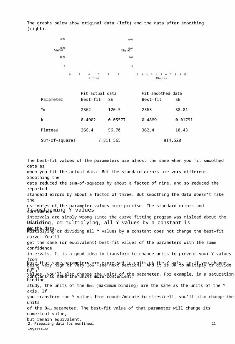
The graphs below show original data (left) and the data after smoothing (right).

3000

2000

1000

0

0 2 4 6 8 10

3000

2000

1000

0

0 1 2 3 4 5 6 7 8 9 10

Signal

Mintues

Signal

Minutes

Fit actual data Fit smoothed dataParameter

Y0

Best-fit

2362

0.4902

366.4

SE

120.5

0.05577

56.70

Best-fit

2363

0.4869

362.4

SE

38.81

0.01791

18.43

814,520

k

Plateau

Sum-of-squares 7,811,565

The best-fit values of the parameters are almost the same when you fit smoothed data aswhen you fit the actual data. But the standard errors are very different. Smoothing thedata reduced the sum-of-squares by about a factor of nine, and so reduced the reportedstandard errors by about a factor of three. But smoothing the data doesn’t make theestimates of the parameter values more precise. The standard errors and confidenceintervals are simply wrong since the curve fitting program was mislead about the scatterin the data.

Transforming Y values

Dividing, or multiplying, all Y values by a constant is OK.Multiplying or dividing all Y values by a constant does not change the best-fit curve. You’llget the same (or equivalent) best-fit values of the parameters with the same confidenceintervals. It is a good idea to transform to change units to prevent your Y values frombeing very high or very low (see next section). And it is OK to multiply or divide by aconstant to make the units more convenient.

Note that some parameters are expressed in units of the Y axis, so if you change the Yvalues, you’ll also change the units of the parameter. For example, in a saturation bindingstudy, the units of the Bmax (maximum binding) are the same as the units of the Y axis. Ifyou transform the Y values from counts/minute to sites/cell, you’ll also change the unitsof the Bmax parameter. The best-fit value of that parameter will change its numerical value,but remain equivalent.


Subtracting a constant is OKSubtracting a constant from all Y values will not change the distance of the points fromthe best-fit curve, so will not affect which curve gets selected by nonlinear regression.

Think carefully about nonlinear transformsAs mentioned above, transforming Y values with a linear transformation (such as dividingall values by a constant, or subtracting a constant from all values), won't change thenature of the best-fit curve. In contrast, nonlinear transformations (such as converting Yvalues to their logarithms, square roots, or reciprocals) will change the relative position ofdata points from the curve and cause a different curve to minimize the sum-of-squares.Therefore, a nonlinear transformation of Y values will lead to different best-fit parametervalues. Depending on the data, this can be good or bad.

Nonlinear regression is based on the assumption that the scatter of data around the curvefollows a Gaussian distribution. If the scatter of your data is in fact Gaussian, performinga nonlinear transform will invalidate your assumption. If you have data with Gaussianscatter, avoid nonlinear Y transforms. If, however, your scatter is not Gaussian, anonlinear transformation might make the scatter more Gaussian. In this case, it is a goodidea to apply nonlinear transforms to your Y values.

Change units to avoid tiny or huge valuesIn pure math, it makes no difference what units you use to express your data. When youanalyze data with a computer, however, it can matter. Computers can get confused by verysmall or very large numbers, and round-off errors can result in misleading results.

When possible, try to keep your Y values between about 10-9 and 109, changing units ifnecessary. The scale of the X values usually matters less, but we’d suggest keeping Xvalues within that range as well.

Note: This guideline is just that. Most computer programs will work fine withnumbers much larger and much smaller. It depends on which program andwhich analysis.

NormalizingOne common way to normalize data is to subtract off a baseline and then divide by aconstant. The goal is to make all the Y values range between 0.0 and 1.0 or 0% and 100%.Normalizing your data using this method, by itself, will not affect the results of nonlinearregression. You’ll get the same best-fit curve, and equivalent best-fit parameters andconfidence intervals.

If you normalize from 0% to 100%, some points may end up with normalized values lessthan 0% or greater than 100. What should you do with such points? Your first reactionmight be that these values are clearly erroneous, and should be deleted. This is not a goodidea. The values you used to define 0% and 100% are not completely accurate. And even ifthey were, you expect random scatter. So some points will end up higher than 100% andsome points will end up lower than 0%. Leave those points in your analysis; don’teliminate them.

Don’t confuse two related decisions:


• Should you normalize the data? Normalizing, by itself, will not change thebest-fit parameters (unless your original data had such huge or tiny Y valuesthat curve fitting encountered computer round-off or overflow errors). If younormalize your data, you may find it easier to see what happened in theexperiment and to compare results with other experiments.

Should you constrain the parameters that define bottom and/or top plateausto constant values? Fixing parameters to constant values will change thebest-fit results of the remaining parameters, as shown in the example below.

•

Averaging replicatesIf you collected replicate Y values (say triplicates) at each value of X, you may be temptedto average those replicates and only enter the mean values into the nonlinear regressionprogram. Hold that urge! In most situations, you should enter the raw replicate data. Seepage 87.

Consider removing outliersWhen analyzing data, you'll sometimes find that one value is far from the others. Such avalue is called an outlier, a term that is usually not defined rigorously. When youencounter an outlier, you may be tempted to delete it from the analyses. First, ask yourselfthese questions:

•

•

Was the value entered into the computer correctly? If there was an error indata entry, fix it.

Were there any experimental problems with that value? For example, if younoted that one tube looked funny, you have justification to exclude the valueresulting from that tube without needing to perform any calculations.

Could the outlier be caused by biological diversity? If each value comes froma different person or animal, the outlier may be a correct value. It is anoutlier not because of an experimental mistake, but rather because thatindividual may be different from the others. This may be the most excitingfinding in your data!

•

After answering “no” to those three questions, you have to decide what to do with theoutlier. There are two possibilities.

• One possibility is that the outlier was due to chance. In this case, you shouldkeep the value in your analyses. The value came from the same distributionas the other values, so it should be included.

The other possibility is that the outlier was due to a mistake - bad pipetting,voltage spike, holes in filters, etc. Since including an erroneous value in youranalyses will give invalid results, you should remove it. In other words, thevalue comes from a different population than the others and is misleading.

•

The problem, of course, is that you can never be sure which of these possibilities iscorrect. Statistical calculations can quantify the probabilities.

Statisticians have devised several methods for detecting outliers. All the methods firstquantify how far the outlier is from the other values. This can be the difference between


the outlier and the mean of all points, the difference between the outlier and the mean ofthe remaining values, or the difference between the outlier and the next closest value.Next, standardize this value by dividing by some measure of scatter, such as the SD of allvalues, the SD of the remaining values, or the range of the data. Finally, compute a P valueanswering this question: If all the values were really sampled from a Gaussian population,what is the chance of randomly obtaining an outlier so far from the other values? If thisprobability is small, then you will conclude that the outlier is likely to be an erroneousvalue, and you have justification to exclude it from your analyses.

One method of outlier detection (Grubbs’ method) is described in the companion book,Prism 4 Statistics Guide. No outlier test will be very useful unless you have lots (say adozen or more) replicates.

Be wary of removing outliers simply because they seem "too far" from the rest. All the datapoints in the figure below were generated from a Gaussian distribution with a mean of100 and a SD of 15. Data sets B and D have obvious "outliers". Yet these points came fromthe same Gaussian distribution as the rest. If you removed these values as outliers, themean of the remaining points would be further from the true value (100) rather thancloser to it. Removing those points as "outliers" makes any further analysis less accurate.

150

125

100

75

50

A B C D E F G H I J

Tip: Be wary when removing a point that is obviously an outlier.


3. Nonlinear regression choices

Choose a model for how Y varies with XNonlinear regression fits a model to your data. In most cases, your goal is to get back thebest-fit values of the parameters in that model. If so, it is crucial that you pick a sensiblemodel. If the model makes no sense, even if it fits the data well, you won’t be able tointerpret the best-fit values.

In other situations, your goal is just to get a smooth curve to use for graphing or forinterpolating unknown values. In these cases, you need a model that generates a curvethat goes near your points, and you won’t care whether the model makes scientific sense.

Much of this book discusses how to pick a model, and explains models commonly used inbiology.

If you want to fit a global model, you must specify which parameters are shared amongdata sets and which are fit individually to each data set. This works differently fordifferent programs. See page 70.

Fix parameters to a constant value?As part of picking a model, you need to decide which parameters in the model you will setto a constant value based on control data. For example, if you are fitting an exponentialdecay, you need to decide if the program will find a best-fit value for the bottom plateau orwhether you will set that to a constant value (perhaps zero). This is an important decision,that is best explained through example.

Here are data to be fit to an exponential decay.

125

100

Y=Plateau+Span ⋅ e -k⋅t

Signal75

50

25

0

0 1 2 3 4Time

We fit the data to an exponential decay, asking the computer to fit three parameters, thestarting point, the rate constant, and the bottom plateau. The best-fit curve shown abovelooks fine. But as you can see below, many exponential decay curves fit your data almostequally well.

3. Nonlinear regression choices 25

125

100

Signal75

50

25

0

-25

0 2 4 6 8 10 12Time

The data simply don’t define all three parameters in the model. You didn’t collect data outto long enough time points, so your data simply don’t define the bottom plateau of thecurve. If you ask the program to fit all the parameters, the confidence intervals will be verywide – you won’t determine the rate constant with reasonable precision. If, instead, youfix the bottom parameter to 0.0 (assuming you have normalized the data so it has to endup at zero), then you’ll be able to determine the rate constant with far more precision.

Tip: If your data don’t define all the parameters in a model, try to constrain oneor more parameters to constant values.

It can be a mistake to fix a parameter to a constant value, when that constant value isn’tquite correct. For example, consider the graph below with dose-response data fit twoways. First, we asked the program to fit all four parameters: bottom plateau, top plateau,logEC50 (the middle of the curve) and the slope. The solid curve shows that fit. Next, weused the mean of the duplicates of the lowest concentration to define the bottom plateau(1668), and the mean of the duplicates of the highest concentration to define the topplateau (4801). We asked the program to fix those parameters to constant values, andonly fit logEC50 and slope. The dashed curve shows the results. By chance, the responseat the lowest concentration was a bit higher than it was for the next two concentrations.By forcing the curve to start at this (higher) value, we pushed the logEC50 to the right.When we fit all four parameters, the best-fit value of the logEC50 was -6.00. When wefixed the top and bottom plateaus to constant values, the best-fit value of the logEC50 was-5.58.

5000

Response2500

0

10 -9 10 -8 10 -7 10 -6 10 -5 10 -4 10 -3Dose

In this example, fixing parameters to constant values (based on control measurements)was a mistake. There are plenty of data points to define all parts of the curve. There is no


need to define the plateaus based on duplicate determinations of response at the lowestand highest dose.

Tip: If you are going to constrain a parameter to a constant value, make sureyou know that value quite accurately.

Initial valuesNonlinear regression is an iterative procedure. The program must start with estimatedinitial values for each parameter. It then adjusts these initial values to improve the fit.

If you pick an equation built into your nonlinear regression program, it will probablyprovide initial values for you. If you write your own model, you’ll need to provide initialvalues or, better, rules for computing the initial values from the range of the data.

You'll find it easy to estimate initial values if you have looked at a graph of the data,understand the model, and understand the meaning of all the parameters in the equation.Remember that you just need estimated values. They don't have to be very accurate.

If you are having problems estimating initial values, set aside your data and simulate afamily of curves (in Prism, use the analysis “Create a family of theoretical curves”). Onceyou have a better feel for how the parameters influence the curve, you might find it easierto go back to nonlinear regression and estimate initial values.

Another approach to finding initial values is to analyze your data using a linearizingmethod such as a Scatchard or Lineweaver-Burk plot. While these methods are obsoletefor analyzing data (see page 19), they are reasonable methods for generating initial valuesfor nonlinear regression. If you are fitting exponential models with multiple phases, youcan obtain initial values via curve stripping (see a textbook of pharmacokinetics fordetails).

Page 43 shows an example where poor initial values prevent nonlinear regression fromfinding best-fit values of the parameters.

WeightingThe goal of regression is to find best-fit values for the parameters of the model (e.g., slopeand intercept for linear regression, other parameters, such as rate constants, for nonlinearregression). More precisely, the goal is the find values for the parameters that are mostlikely to be correct. It turns out that you can’t decide which parameter values are mostlikely to be correct without first making an assumption about how the data are scatteredaround the line or curve.

Most commonly, linear and nonlinear regression make two assumptions:

•

•

The scatter follows a Gaussian (also called a “normal”) distribution.

The standard deviation of the scatter (the average amount of scatter) is thesame for all values of X.

Given these two assumptions, how does nonlinear regression decide which parametervalues are most likely to be correct? The answer, discussed in more detail in Chapter 13, isthat the parameters that are most likely to be correct are those that generate a curve that

3. Nonlinear regression choices 27

minimizes the sum of the squares of the vertical distance between data points and curve.In other words, least-squares regression minimizes:

∑(Y Data-YCurve ) 2

If the scatter really is Gaussian and uniform, least-squares regression finds the parametervalues that are most likely to be correct.

It is possible to change the first assumptions, and make some other assumption about thescatter. But the Gaussian assumption works well, and is used for almost all curve fitting.The only real exception is robust nonlinear regression, designed to reduce the influence ofoutliers, which uses different assumptions.

GraphPad note: Prism 4 does not perform robust nonlinear regression, but thenext version almost certainly will.

The second assumption is that the average amount of scatter is the same all the way alongthe curve, at all values of X. This assumption is often not true. Instead, the averageamount of scatter often increases as Y increases. With this kind of data, a least-squaresmethod tends to give undue weight to the points with large Y values, and ignores pointswith low Y values. To prevent this, it is common to apply a weighting scheme.

The most common alternative to minimizing the sum of the squares of the verticaldistances of the points from the curve, is to minimize the sum of the squares of therelative distances of the points from the curve. In other words, minimize this quantity:

YData -YCurve ∑ YData

2

This is called relative weighting or weighting by 1/Y2.

If you know that the scatter is not uniform, you should choose an appropriate weightingscheme. Often it will be hard to know what weighting scheme is appropriate. Fortunately,it doesn’t matter too much. Simulations have shown that picking the wrong weightingscheme, while making the best-fit values less accurate, doesn’t make as large an impact asyou might guess.

If you collected replicate values at each value of X, you might be tempted to weight by thestandard deviation of the replicates. When replicates are close together with a smallstandard deviation, give that point lots of weight. When replicates are far apart, and havea large standard deviation, give that point little weight. While this sounds sensible, itactually doesn’t work very well. To see why, read the section starting on page 87.

See Chapter 14 for more information on unequal weighting of data points.

Other choicesYour program will give you lots of choices for additional calculations, and for how youwant to format the results. For GraphPad Prism, see Chapters 45 to 47. If you are new tononlinear regression, leave all these settings to their default values, and spend your timelearning about models and about interpreting the results. Then go back and learn aboutthe various options.


4. The first five questions to ask aboutnonlinear regression results

Nonlinear regression programs can produce lots of output, and it can be hard to knowwhat to look at first. This chapter explains the first five questions you should ask wheninterpreting nonlinear regression results. The next chapter explains the rest of the results.

Does the curve go near your data?The whole point of nonlinear regression is to fit a model to your data – to find parametervalues that make the curve come near your data points. The first step in evaluating theresults, therefore, is to look at a graph of your data with the superimposed curve.

Tip: Don’t neglect this first step. Look at your data with the superimposedcurve.

If your goal is simply to create a standard curve from which to interpolate unknownvalues, it may be enough to look at the curve. You may not care about the best-fit values ofthe parameters and their standard errors and confidence intervals. More commonly,however, you will be fitting curves to your data in order to understand your system. Underthis circumstance, you need to look carefully at the nonlinear regression results.Nonlinear regression generates quite a few results, and the rest of this chapter is guide tointerpreting them.

Are the best-fit parameter values plausible?When evaluating the parameter values reported by nonlinear regression, the first thing todo is check that the results are scientifically plausible. When a computer program fits amodel to your data, it can’t know what the parameters mean. Therefore, it can report best-fit values of the parameters that make no scientific sense. For example, make sure thatparameters don’t have impossible values (rate constants simply cannot be negative).Check that EC50 values are within the range of your data. Check that maximum plateausaren’t too much higher than your highest data point.

If the best-fit values are not scientifically sensible, then the fit is no good. Considerconstraining the parameters to a sensible range, and trying again.

For help with troubleshooting results that just don’t make sense, see Chapter 6.

How precise are the best-fit parameter values?You don’t just want to know what the best-fit value is for each parameter. You also want toknow how certain that value is.

Nonlinear regression programs report the standard error of each parameter, as well as the95% confidence interval. If your program doesn’t report a 95% confidence interval, youcan calculate one using the equation on page 103. Or you can quickly estimate theconfidence interval as the best-fit value plus or minus two standard errors.

4. The first five questions to ask about nonlinear regression results 29

If all the assumptions of nonlinear regression are true, there is a 95% chance that theinterval contains the true value of the parameter. If the confidence interval is reasonablynarrow, you’ve accomplished what you wanted to do – found the best fit value of theparameter with reasonable certainty. If the confidence interval is really wide, then you’vegot a problem. The parameter could have a wide range of values. You haven’t nailed itdown. See Chapter 6 for troubleshooting tips.

Note that the confidence interval and standard error are calculated from one experimentbased on the scatter of the points around the curve. This gives you a sense of how well youhave determined a parameter. But before making any substantial conclusions, you’ll wantto repeat the experiment. Then you can see how the parameter varies from experiment toexperiment. This includes more sources of experimental variation than you see in a singleexperiment.

For details, see part E. Confidence intervals of the parameters.

Tip: The standard errors and confidence intervals are important results ofregression. Don’t overlook them.

Would another model be more appropriate?Nonlinear regression finds parameters that make a model fit the data as closely aspossible (given some assumptions). It does not automatically ask whether another modelmight work better. You can compare the fit of models as explained beginning in Chapter21.

Even though a model fits your data well, it may not be the best, or most correct, model.You should always be alert to the possibility that a different model might work better. Insome cases, you can’t distinguish between models without collecting data over a widerrange of X. In other cases, you would need to collect data under different experimentalconditions. This is how science moves forward. You consider alternative explanations(models) for your data, and then design experiments to distinguish between them.

Have you violated any of the assumptions of nonlinearregression?Nonlinear regression is based on a set of assumptions. When reviewing your results,therefore, you should review the assumptions and make sure you have not violated them.

•

•

X is known precisely. All the “error” (scatter) is in Y.

The variability of Y values at any particular X value follows a knowndistribution. Almost always, this is assumed to be a Gaussian (normal) bell-shaped distribution.

Standard nonlinear regression assumes that the amount of scatter (the SD ofthe residuals) is the same all the way along the curve. This assumption ofuniform variance is called homoscedasticity. Weighted nonlinear regressionassumes that the scatter is predictably related to the Y value. See Chapter 14.

The observations are independent. When you collect a Y value at a particularvalue of X, it might be higher or lower than the average of all Y values at thatX value. Regression assumes that this is entirely random. If one point


•

•

30

happens to have a value a bit too high, the next value is equally likely to betoo high or too low.

If you choose a global model, you also are making two additional assumptions (see page69):

• All data sets are expressed in same units. If different data sets wereexpressed in different units, you could give different data sets differentweights just by expressing the values in different units.

The scatter is the same for each data set. At each X value, for each data set,the scatter should be the same (unweighted fit) or should vary predictablywith Y (and be accounted for by weighting).

•

4. The first five questions to ask about nonlinear regression results 31

5. The results of nonlinear regression

The previous chapter discussed the five most important questions to ask when reviewingresults of nonlinear regression. This chapter explains the rest of the results.

Confidence and prediction bandsThe plot of the best-fit curve can include the 95% confidence band of the best-fit curve, orthe 95% prediction band. The two are very different.

1500 1500

Response Response1000 1000

500 500

95% confidence band

0

-9 -8 -7 -6 -5 -4 -3

95% prediction band

0

-9 -8 -7 -6 -5 -4 -3log(Dose) log(Dose)

The confidence band tells you how well you know the curve. You can be 95% sure that thetrue best-fit curve (which you could only know if you had an infinite number of datapoints) lies within the confidence band.

The prediction band shows the scatter of the data. If you collected many more data points,you would expect 95% to fall within the prediction band.

Since the prediction band has to account for uncertainty in the curve itself as well asscatter around the curve, the prediction band is much wider than the confidence band. Asyou increase the number of data points, the confidence band gets closer and closer to thebest-fit curve, while the prediction band doesn’t change predictably. In the examplebelow, note that the confidence bands (shown as solid) contain a minority of the datapoints. That’s ok. The confidence bands have a 95% chance of containing the true best-fitcurve, and with so much data these bands contain far fewer than half the data points. Incontrast, the dashed prediction bands include 95% of the data points.

2000

1000Y

0

-9 -8 -7 -6 -5 -4 -3X


Correlation matrixIf the standard errors are large (so the confidence intervals are wide), you’ll want toinvestigate further. One possibility is that the model is somewhat redundant, so twoparameters are linked. Some programs report a correlation matrix to help diagnose thisproblem.

For every pair of parameters, the correlation matrix reports a value showing you howtightly those two parameters are linked. This value is like a correlation coefficient, rangingin value from -1 to +1.

The program finds the best fit values of each parameter. That means that if you change thevalue of any parameter (without changing the rest), the sum of squares will go up (the fitwill be worse). But what if you change the value of one parameter and fix it, and then askthe program to find a new best-fit value for another parameter? One extreme is when theparameters are completely unlinked. Changing one parameter makes the fit worse, andyou can’t compensate at all by changing the other. In this extreme case, the value reportedby the correlation matrix would be zero. The other extreme is when the two parametersare completely intertwined. Changing one parameter makes the fit worse, but this can becompletely compensated for by changing the other. The value reported in the correlationmatrix would be +1 (if you compensate for an increase in one parameter by increasing theother) or -1 (if you compensate for an increase in one parameter by decreasing the other).

Parameters in most models are somewhat related, so values in the range -0.8 to + 0.8 areseen often. Higher correlations (greater than 0.9, and especially greater than 0.99, orlower than -0.9 or -0.99) mean that data simply don’t define the model unambiguously.One way to solve this problem is to simplify the model, perhaps by fixing a parameter to aconstant value. Another solution is to collect more data (either use a wider range of Xvalues, or include data from another kind of experiment in a global fit).

GraphPad note: Prism does not report the correlation matrix. Let us know ifyou’d like to see the covariance matrix in future versions.

Sum-of-squares

Sum-of-squares from least squares nonlinear regressionThe sum-of-squares (SS) is the sum of the squares of the vertical distances of the pointsfrom the curve. It is expressed in the units used for the Y values, squared. Standard (leastsquares) nonlinear regression works by varying the values of the model parameters tominimize SS. If you chose to weight the values and minimize the relative distance squared(or some other weighting function), goodness-of-fit is quantified with the weighted sum-of-squares.

You’ll only find the SS value useful if you do additional calculations to compare models.

Sy.x (Root mean square)The equation below calculates the value, sy.x, from the sum-of-squares and degrees offreedom:

s y⋅x =

5. The results of nonlinear regression

SSN-P

33

Sy.x is the standard deviation of the vertical distances of the points from the line, N is thenumber of data points, and P is the number of parameters. Since the distances of thepoints from the line are called residuals, sy.x is the standard deviation of the residuals. Itsvalue is expressed in the same units as Y. Some programs call this value se.

R2 (coefficient of determination)The value R quantifies goodness of fit. R2 is a fraction between 0.0 and 1.0, and has nounits. Higher values indicate that the curve comes closer to the data. You can interpret R2from nonlinear regression very much like you interpret r2 from linear regression. Bytradition, statisticians use uppercase (R2) for the results of nonlinear and multipleregressions and lowercase (r2) for the results of linear regression, but this is a distinctionwithout a difference.

When R equals 0.0, the best-fit curve fits the data no better than a horizontal line goingthrough the mean of all Y values. In this case, knowing X does not help you predict Y. 2When R =1.0, all points lie exactly on the curve with no scatter. If you know X, you can 2calculate Y exactly. You can think of R as the fraction of the total variance of Y that is ex-plained by the model (equation).

Tip: Don't make the mistake of using R2 as your main criterion for whether a fitis reasonable. A high R2 tells you that the curve came very close to the points,but doesn’t tell you that the fit is sensible in other ways. The best-fit values ofthe parameters may have values that make no sense (for example, negative rateconstants) or the confidence intervals may be very wide.

R2 is computed from the sum of the squares of the distances of the points from the best-fitcurve determined by nonlinear regression. This sum-of-squares value is called SSreg, whichis in the units of the Y-axis squared. To turn R2 into a fraction, the results are normalizedto the sum of the square of the distances of the points from a horizontal line through themean of all Y values. This value is called SStot. If the curve fits the data well, SSreg will bemuch smaller than SStot.

The figure below illustrates the calculation of R2. Both panels show the same data andbest-fit curve. The left panel also shows a horizontal line at the mean of all Y values, andvertical lines show how far each point is from the mean of all Y values. The sum of thesquare of these distances (SStot) equals 62735. The right panel shows the vertical distanceof each point from the best-fit curve. The sum of squares of these distances (SSreg) equals4165.

2

2


R2 is calculated using this equation:

R 2 =1.0-SSreg

SStot=1.0-

4165 =1.0-0.0664=0.933662735

Note that R2 is not really the square of anything. If SSreg is larger than SStot, R2 will benegative. While it is surprising to see something called "squared" have a negative value, itis not impossible (since R2 is not actually the square of R). R2 will be negative when thebest-fit curve fits the data worse than a horizontal line at the mean Y value. This couldhappen if you pick an inappropriate model (maybe you picked an exponential associationmodel rather than an exponential dissociation model), or enforce an inappropriateconstraint (for example, if you fix the Hill slope of a dose-response curve to 1.0 when thecurve goes downhill).

Warning: If you want to compare the fit of two equations, don't just compare R2values. Comparing curves is more complicated than that.

Does the curve systematically deviate from the data?If you've picked an appropriate model, and your data follow the assumptions of nonlinearregression, the data will be randomly distributed around the best-fit curve. You can assessthis in three ways:

•

•

•

The distribution of points around the curve should be Gaussian.

The average distance of points from curve should be the same for all parts ofthe curve (unless you used weighting).

Points should not be clustered. Whether each point is above or below thecurve should be random.

Residuals and runs help you evaluate whether the curve deviates systematically from yourdata.

Residuals from nonlinear regressionA residual is the distance of a point from the curve. A residual is positive when the point isabove the curve, and is negative when the point is below the curve. If you listed theresiduals of a particular curve fit in the form of a table, you would use the same X valuesas the original data, but the Y values would be the vertical distances of each correspondingpoint from the curve.

A sample residual plot is shown below. If you look carefully at the curve on the left, you’llsee that the data points are not randomly distributed above and below the curve. Thereare clusters of points at early and late times that are below the curve, and a cluster ofpoints at middle time points that are above the curve. This is much easier to see on thegraph of the residuals in the inset. The data are not randomly scattered above and belowthe X-axis.

5. The results of nonlinear regression 35

50

200

Residual25

0

-25Signal100-50

0

0 10 20 30

Time40 50 60

Runs test from nonlinear regressionThe runs test determines whether the curve deviates systematically from your data. A runis a series of consecutive points that are either all above or all below the regression curve.Another way of saying this is that a run is a consecutive series of points whose residualsare either all positive or all negative.

If the data points are randomly distributed above and below the regression curve, it ispossible to calculate the expected number of runs. If there are Na points above the curveand Nb points below the curve, the number of runs you expect to see equals[(2NaNb)/(Na+Nb)]+1. In most cases, you’ll find about equal number of points above andbelow the curve, so Na and Nb each equal N/2, where N is the total number of points. Withthis approximation, the rule is that you expect to see about 1+ N/2 runs.

If you observe fewer runs than expected, it may be a coincidence or it may mean that youpicked an inappropriate regression model and the curve systematically deviates from yourdata. The P value from the runs test answers this question: If the data really follow themodel you selected, what is the chance that you would obtain as few (or fewer) runs asobserved in this experiment?

The P values are always one-tailed, asking about the probability of observing as few runs(or fewer) than observed. If you observe more runs than expected, the P value will behigher than 0.50.

If the runs test reports a low P value, conclude that the data don’t really follow theequation you have selected.

In the example above, you expect 21 runs. There are 13 runs, and the P value for the runstest is 0.0077. If the data were randomly scattered above and below the curve, there is lessthan a 1% chance of observing so few runs. The data systematically deviate from the curve.Most likely, the data were fit to the wrong equation.


Testing whether the residuals are GaussianLeast-squares nonlinear regression (as well as linear regression) assumes that thedistribution of residuals follows a Gaussian distribution (robust nonlinear regression doesnot make this assumption). You can test this assumption by using a normality test on theresiduals. This test is usually available in a many statistical and some curve-fittingprograms.

GraphPad note: Prism allows you to test whether your data or residuals follow aGaussian distribution by performing a normality test on the residuals. From theresidual table, click Analyze and choose Column Statistics. Then choose anormality test as part of the Column Statistics analysis.

Could the fit be a local minimum?The nonlinear regression procedure adjusts the parameters in small steps in order toimprove the goodness-of-fit. If the procedure converges on an answer, you can be surethat altering any of the variables a little bit will make the fit worse. But it is theoreticallypossible that large changes in the variables might lead to a much better goodness-of-fit.Thus the curve that nonlinear regression decides is the “best” may really not be the best.

Start here and resultwill be a false minimum.

Start here and resultwill be the best fit.

Sum-of-squares

False MinimumBest Fit

Value of Variable

Think of latitude and longitude as representing two parameters you are trying to fit. Nowthink of altitude as the sum-of-squares. Nonlinear regression works iteratively to reducethe sum-of-squares. This is like walking downhill to find the bottom of the valley. See page91. When nonlinear regression has converged, changing any parameter increases thesum-of-squares. When you are at the bottom of the valley, every direction leads uphill.But there may be a much deeper valley over the ridge that you are unaware of. Innonlinear regression, large changes in parameters might decrease the sum-of-squares.

This problem (called finding a local minimum) is intrinsic to nonlinear regression, nomatter what program you use. You will rarely encounter a local minimum if you havecollected data with little scatter and over an appropriate range of X values, have chosenan appropriate equation, and have provided a sensible initial value for each parameter.

To test for the presence of a false minimum, run nonlinear regression several times. Eachtime, provide a different set of initial values. If these fits all generate the same parametervalues, with the same sum-of-squares, you can be confident you have not encountered afalse minimum.

5. The results of nonlinear regression 37

6. Troubleshooting “bad” fits

This chapter shows you five examples of bad fits, and explains what went wrong in eachone and how the analysis can be salvaged.

Poorly defined parametersBest-fit values BOTTOM TOP LOGEC50 HILLSLOPE EC50Std. Error BOTTOM TOP LOGEC50 HILLSLOPE95% Confidence Intervals BOTTOM TOP LOGEC50 HILLSLOPE EC50Goodness of Fit Degrees of Freedom RІ Absolute Sum of Squares Sy.x

-23.19137.2-7.8370.58391.4560e-008

82.06119.10.63150.8777

-1066 to 1019-1376 to 1650-15.86 to 0.1870-10.57 to 11.741.3783e-016 to 1.538

10.987671.078.431

100

Response50

0

-9 -8 -7log(dose, M)

In this example, a response was measured at five concentrations, and the results were fitto a sigmoidal dose-response curve with variable slope, also called a four-parameterlogistic equation or the Hill equation.

When you first look at the results, all may seem fine. The R2 is high, and both the logEC50and the Hill slope have reasonable best-fit values.

A closer look shows you the trouble. The confidence interval of the EC50 spans 15 orders ofmagnitude (ranging from homeopathy to insolubility). The confidence interval for the HillSlope is also extremely wide, extending from -11 (a steep curve heading down as you gofrom left to right) to +12 (a steep curve heading up hill). With such wide confidenceintervals, the curve fit is not at all helpful.

Tip: Always look at the confidence intervals for best-fit values. If the confidenceintervals are extremely wide, the fit is not likely to be very helpful.

The problem is clear once you think about it. Nonlinear regression was asked to fit fourparameters - the bottom plateau, the top plateau, logEC50 and Hill slope. But the datadon’t extend far enough to define the bottom and top plateaus. Since the top and bottomare not defined precisely, neither is the middle, so the logEC50 is very imprecise.

It is easy to salvage this experiment and get useful results. Since the data were normalizedto run from 0 to 100, there is no need to ask the nonlinear regression program to fit thebest-fit values of the Bottom and Top. Instead, constrain Bottom to equal 0 and Top to


equal 100. Now you only have to ask the program to fit two parameters (logEC50 andslope). Here are the revised results.

Best-fit values BOTTOM TOP LOGEC50 HILLSLOPE EC50Std. Error LOGEC50 HILLSLOPE95% Confidence Intervals LOGEC50 HILLSLOPE EC50Goodness of Fit Degrees of Freedom RІ Absolute Sum of Squares Sy.x

0.0100.0-7.9891.1291.0257e-008

0.066440.1789

-8.200 to -7.7780.5603 to 1.6996.3036e-009 to 1.6689e-008

30.9802114.16.168

100

Response50

0

-9 -8 -7

log(dose, M)

The confidence interval of the logEC50 extends plus or minus 0.2 log units, so the EC50 isknown within a factor of 1.6 (the antilog of 0.2) . Since the curve is defined by so fewpoints, the Hill Slope is still not defined very well, but the confidence interval is muchnarrower than it was before.

Tip: If your data are normalized in any way, think carefully about whether anyof the parameters in the equation you selected can be fixed to a constant value.

Model too complicated BOTTOM TOP FRACTION1 LOGEC50_1 LOGEC50_2 EC50_1 EC50_295% Confidence Intervals BOTTOM TOP FRACTION1 LOGEC50_1 LOGEC50_2 EC50_1 EC50_2Goodness of Fit Degrees of Freedom RІ Absolute Sum of Squares Sy.x

-3.759101.50.8775-5.922-5.9061.1979e-0061.2423e-006

-8.168 to 0.649897.60 to 105.30.0 to 1.000-496.7 to 484.9-3532 to 3520

100

Response50

0

-8 -7 -6log[dose, M]

-5 -4100.997561.882.488

This example shows results of a competitive binding assay. The nonlinear regression fit atwo-component competitive binding curve in order to find the two LogEC50 values and therelative fraction of each component.

The curve follows the data nicely, so R2 is high. But look closer and you’ll see some majorproblems. The confidence interval for the parameter fraction (the fraction of sites that areof high-affinity) ranges from 0 to 1 – all possible values. The two log EC50 values arealmost identical with extremely wide confidence intervals. With such wide confidenceintervals, this fit is not helpful.

6. Troubleshooting “bad” fits 39

Part of the problem is the same as with example 1. These data were normalized to runfrom 0 to 100, so the values of Bottom and Top ought to be constrained to those values.Here are the revised results.

100

Response

50

0


-5 -4

Best-fit values BOTTOM TOP FRACTION1 LOGEC50_1 LOGEC50_2 EC50_1 EC50_295% Confidence Intervals FRACTION1 LOGEC50_1 LOGEC50_2 EC50_1 EC50_2Goodness of Fit Degrees of Freedom RІ Absolute Sum of Squares Sy.x

0.0100.01.000-5.932-38.401.1687e-0060.0000e+000

0.0 to 1.000-7.689 to -4.175-8536000 to 8.5356e+0062.0448e-008 to 6.6797e-005

120.9947132.03.317

The curve still looks fine, and now the results look better, at first glance. But theconfidence interval for the logEC50 of the second site is extremely wide. This is because thebest-fit value of the parameter fraction is 100%, meaning that all the sites are of the firsttype. Of course the confidence interval for the second site is wide, if the program isn’tconvinced that that site even exists.

Is there any evidence for the existence of this second site? Here are the results fitting it toa one-site competitive binding model, constraining the Bottom and Top to 0 and 100.

Best-fit values BOTTOM TOP LOGEC50 EC50Std. Error LOGEC5095% Confidence Intervals LOGEC50 EC50Goodness of Fit Degrees of Freedom RІ Absolute Sum of Squares Sy.x

0.0100.0-5.9471.1289e-006

0.02617

-6.004 to -5.8919.9197e-007 to 1.2846e-006

140.9948128.83.033

100

Response50

0


-5 -4

The sum-of-squares is a bit lower with the one-site fit than two two-site fit. And the one-site fit has a logEC50 value with a narrow (useful) confidence interval. There simply isnothing in the data to suggest the presence of a second site. When you fit two sites, theprogram complies with your request, but the results are nonsense.

It is possible to compare two models statistically (see Chapter 21), but there is no point ina statistical comparison when the fit of one of the models (the two-site model in thisexample) simply makes no sense.


Tip: Don’t fit a complicated (i.e. two sites or phases) model if a simpler modelfits the data just fine.

The model is ambiguous unless you share a parameter

3000

Response (DPM)

ControlTreated

2000

1000

0-13 -12 -11 -10 -9 -8 -7 -6 -5

log(concentration, M)

This example shows dose-response data for two experimental conditions, where theresults were measured as the generation of a radiolabeled intracellular second messenger.Here are the results of fitting each curve to a variable slope dose-response curve.

ControlBest-fit values

Bottom

Top

Logec50

Hillslope

Ec50

95% ConfidenceIntervals

Bottom

Top

Logec50

Hillslope

Ec50

70.26 to 296.1

1648 to 1829

-9.506 to -9.141

0.5626 to 1.086

3.1220e-010 to7.2350e-010

179.5 to 361.2

-4541 to 11815

-9.414 to -1.682

0.09042 to 0.8450

3.8550e-010 to0.02079

183.2

1739

-9.323

0.8244

4.7520e-010

270.4

3637

-5.548

0.4677

2.8310e-006

Treated

The fit of the control data is OK, although we’d prefer a narrower confidence interval forthe bottom plateau. And since the bottom is a bit uncertain, so is the middle, resulting in aconfidence interval for the EC50 that is wider than we’d like.

The fit of the treated data is not satisfactory at all. The confidence intervals are so widethat you really can’t conclude anything. This is not surprising. The treated data don’tbegin to plateau at high concentrations, so the best-fit value of the top plateau is very


uncertain. The middle of the curve is defined by the top and bottom, so the EC50 is veryuncertain as well.

One solution would be to normalize all the data from 0 to 100 and fix the top and bottomplateaus at those values. But in these experiments, we don’t have good control datadefining the bottom and top. A better alternative is to use global fitting. If we are willing toassume that both curves have the same bottom, top and slope, we can use nonlinearregression to find one best-fit value for those parameters for both data sets, and to findindividual EC50 values for each data set. This assumes that while the treatment may affectthe EC50 (this is what we want to find out), the treatment does not affect the basal ormaximum responses or the steepness (slope) of the curve.

Here are the results.

ControlBest-fit values

Bottom (Shared)

Top (Shared)

LogEC50

Hillslope (Shared)

EC50

95% Confidence IntervalsBottom (Shared)

Top (Shared)

LogEC50

Hillslope (Shared)

EC50

211.7 to 323.3

1656 to 1840

-9.409 to -9.047

0.6254 to 1.007

3.9000e-010 to8.9780e-010

211.7 to 323.3

1656 to 1840

-7.026 to -6.662

0.6254 to 1.007

9.4110e-008 to2.1770e-007

267.5

1748

-9.228

0.8162

5.9170e-010

267.5

1748

-6.844

0.8162

1.4310e-007

Treated

The parameter Bottom is now determined by both data sets, so has a narrower confidenceinterval. The parameter Top is also shared, so the nonlinear regression algorithm is ableto come up with a reasonable best-fit value and confidence interval. Since both the topand bottom are now determined with a reasonable degree of certainty, the middle of thecurve is also determined reasonably well. The program was able to fit EC50 values for bothcurves, with reasonable values and acceptably narrow confidence intervals.

This analysis only worked because we assumed that the treatment changed the logEC50without changing the bottom, top or slope of the curve. Whether this assumption isreasonable depends on the scientific context of the experiment.

The key decision here was to share the value of the parameter Top. Sharing the Bottomand HillSlope helped narrow the confidence intervals, but was not essential.

Tip: When fitting a family of curves, think carefully about whether it makessense to share the value of some parameters among data sets.


Bad initial values

3000

Response2000

1000

0

10 -9 10 -8 10 -7 10 -6 10 -5 10 -4 10 -3Dose (M)

This dose response curve was fit to the equation below, a sigmoidal dose-response curvethat fit the parameter pEC50 rather than logEC50 . The pEC50 is an alternative way ofexpressing the concentration giving the middle of the curve. It equals -1 times thelogEC50).

Y = Bottom + (Top-Bottom)/(1+10^((-pEC50 - X)*HillSlope))

Nonlinear regression failed to fit the model to the data. Instead it reports “Does notconverge”.

The data look fine. The equation was entered properly. What could be wrong? To helpdiagnose the problem, plot the curve generated by the initial values.

3000

Response2000

1000

0

10 -9 10 -7 10 -5 10 -3 10 -1 10 1 10 3 10 5 10 7 10 9

Dose (M)

Oops. Why is the curve so far from the points? Review the rules entered for initial values.


Now the problem is apparent. The initial value of the pEC50 was set equal to the average ofthe lowest (-9) and highest (-3) X values, or -6. But the equation is written in terms of thepEC50, not the logEC50. The initial value for the pEC50 should have been about 6, not -6.This mistake ensured that the curve generated by the initial values is quite far from thedata points, so far that the program is stuck. You can see why. If the program changes thevalue of pEC50 to make it a bit larger (the curve farther to the left) or a bit smaller (thecurve farther to the right) the sum-of-squares doesn’t change. All the data points areunder the top plateau of the curve defined by the initial values. Since the sum-of-squaresdoesn’t change with small changes in the pEC50 value, the program has no clue aboutwhich way it should go. It doesn’t know if the initial value of pEC50 is too high or too low.Since it is stuck, the program reports “Does not converge”. It would need to make muchlarger changes in the value of pEC50 to affect the sum-of-squares, but the nonlinearregression procedure doesn’t do this.

The solution is clear – use better initial values. We change the rule for the initial value ofpEC50 to -1 times the XMID, which is 6. Now the curve generated by the initial values isclose to the points, and curve fitting proceeds without problem.

3000

Response2000

1000

0

10 -9 10 -8 10 -7 10 -6 10 -5 10 -4 10 -3Dose (M)

Tip: If nonlinear regression won’t converge on a best-fit solution, graph thecurve generated by the initial values, and change those initial values if the curveis far from the data.


Redundant parameters

3000

2000CPM

1000

0

0 25 50 75Minutes

This example shows the kinetics of association binding. We attempted to fit it to thisequation, where X is time. For details about this kind of experiment, see page 234.

Y = Ymax 1- e( − (LigandЧk on +k off )ЧX)The parameter Ligand is the concentration of radioactively labeled ligand used in theexperiment. That is set by the experimenter, so we constrain Ligand to a constant value,and ask nonlinear regression to find best-fit values for Ymax, kon and koff.

The nonlinear regression program gives an error message such as “Bad model”. But themodel is correct – that equation describes the kinetics of ligand binding. To check that theproblem was unreasonable initial values, let’s graph the curve defined by the initial values.

3000

2000CPM

1000LIGANDKONKOFFYMAX

1.0000e1.0000e0.01002000

0

0 25 50 75Minutes

While that is hardly a best-fit curve, it does come quite close to the points, close enoughfor curve fitting to work. So why does nonlinear regression fail? Look more carefully atthe equation. Note the term Ligand×Kon+Koff. Ligand is a constant, but we are trying tofit both Kon and Koff from one experiment. The data simply don’t define both values. Youcan see that if the value of Kon is reduced a bit, the curve will be exactly the same if thevalue of Koff is increased. There is no way to fit one set of data to determine values of bothKon and Koff – the answer is ambiguous. We are trying to fit a model that simply is notentirely defined by our data.


The simplest way to solve this problem is to determine the value of Koff from a separatedissociation experiment. Let’s say its value is 0.0945. Now we can constrain Koff to be aconstant with that value, and the curve fitting can proceed. Here are the results:

3000 Best-fit values LIGAND KON KOFF YMAX Std. Error KON YMAX 95% Confidence Intervals KON YMAX Goodness of Fit Degrees of Freedom RІ75 Absolute Sum of Squares Sy.x

1.0000e-0096.9075e+0070.009452336

4.5071e+00632.67

5.9845e+007 to 7.8306e+0072269 to 2402

280.9772316408106.3

2000CPM

1000

0

0 25 50Minutes

It is possible to determine the values of both Kon and Koff, just not from one data set. Todo this, fit a family of association curves (each with a different concentration ofradioligand) and share the values of Kon and Koff among all the data sets. See page 236. Arelated approach is to simultaneously analyze association and dissociation experiments.See page 238.

Tips for troubleshooting nonlinear regressionIf your program generates an error message rather than curve fitting results, you probablywon’t be able to make sense of the exact wording of the message. It tells you where in thecurve fitting process the error occurred, but it will rarely help you figure out why the erroroccurred.

Nonlinear regression depends on choosing a sensible model. If you are not familiar withthe model (equation) you chose, take the time to learn about it. If you fit the wrong model,the results won’t be helpful.

It is not enough to just pick a model. You also have to decide which parameters in themodel should be fit by nonlinear regression, and which should be fixed to constant values.Failure to do this is a common cause of nonlinear regression problems.

Successful nonlinear regression requires a reasonable initial value for each parameter. Inother words, the curve generated by those initial values must come close enough to thedata points that the regression procedure can figure out which parameters are too highand which are too low. A vital first step in troubleshooting nonlinear regression is to plotthe curve that results from those initial values. If that curve is far from the data, you’llneed to change the initial values of the parameters. Even if your program picks the initialvalues for you, you still should review them if the fit is problematic.

If the model has several compartments or phases, see if a simpler model (fewercompartments or phases) fits your data.


B. Fitting data with linear regression

7. Choosing linear regression

Linear regression can be viewed as just a special case of nonlinear regression. Anynonlinear regression program can be used to fit to a linear model, and the results will bethe same as if you had chosen linear regression. Because linear regression is usuallyperformed separately from nonlinear regression, we explain linear regression separatelyhere.

The linear regression modelLinear regression fits this model to your data:

Y=intercept+slopeЧX

Y ∆Y∆X

Y intercept

0

Slope=∆Y/∆X

X

The slope quantifies the steepness of the line. It equals the change in Y for each unit changein X. It is expressed in the units of the Y axis divided by the units of the X axis. If the slope ispositive, Y increases as X increases. If the slope is negative, Y decreases as X increases.

The Y intercept is the Y value of the line when X equals zero. It defines the elevation of the line.

Note: Most programs (including GraphPad Prism) offer separate analysischoices for linear and nonlinear regression. That is why we wrote separatechapters for linear regression. But you can enter a linear model into a nonlinearregression program, and it will work fine. Linear regression is just a simpler,special, case.

Don’t choose linear regression when you really want to computea correlation coefficientLinear regression and correlation are related, and it is easy to mix them up.

7. Choosing linear regression 47

Correlation calculations are not actually a kind of regression. This is because correlationcalculations do not find a best-fit line. Instead, correlation quantifies how consistently twovariables vary together. When a change in one variable corresponds closely to a change inthe other, statisticians say that there is a lot of covariation or correlation. The directionand magnitude of correlation is quantified by the correlation coefficient, r. If r is positive,it means that as one variable goes up so does the other. If r is negative, it means that as onevariable goes up, the other variable goes down. The value of r is always between -1 and +1.

Note that the correlation coefficient quantifies the relationship between two variables. Itdoesn’t matter which you call X and which you call Y – the correlation coefficient will bethe same either way. In contrast, linear regression finds the line that best predicts Y fromX, so your choices of which variable to label X and which to label Y will impact the results.

Analysis choices in linear regression

Force the line through the origin?If you choose regression, you may force the line to go through a particular point such asthe origin. In this case, linear regression will determine only the best-fit slope, as theintercept will be fixed. Use this option when scientific theory tells you that the line mustgo through a particular point (usually the origin, X=0, Y=0) and you only want to knowthe slope. This situation arises rarely.

Use common sense when making your decision. For example, consider a protein assay.You measure optical density (Y) for several known concentrations of protein in order tocreate a standard curve. You then want to interpolate unknown protein concentrationsfrom that standard curve. When performing the assay, you adjusted thespectrophotometer so that it reads zero with zero protein. Therefore you might betempted to force the regression line through the origin. But this constraint may result in aline that doesn't fit the data so well. Since you really care that the line fits the standardsvery well near the unknowns, you will probably get a better fit by not constraining the line.

Most often, you should let linear regression find the best-fit line without any constraints.

Fit linear regression to individual replicates or to means?If you collected replicate Y values at every value of X, there are two ways to calculate linearregression. You can treat each replicate as a separate point, or you can average thereplicate Y values, to determine the mean Y value at each X, and do the linear regressioncalculations using the means.

You should consider each replicate a separate point when the sources of experimentalerror are the same for each data point. If one value happens to be a bit high, there is noreason to expect the other replicates to be high as well. The errors are independent.

Average the replicates and treat the mean as a single value when the replicates are notindependent. For example, the replicates would not be independent if they representtriplicate measurements from the same animal, with a different animal used at each valueof X (dose). If one animal happens to respond more than the others, that will affect all thereplicates. The replicates are not independent.

We discuss this topic in more depth on page 87.

48 B. Fitting data with linear regression

X and Y are not interchangeable in linear regressionStandard linear regression calculations are based on the assumption that you know all theindependent (X) values perfectly, and that all of the uncertainty or scatter is in theassessment of the dependent (Y) values. This is why standard linear regression (as well asnonlinear regression) minimizes the sum of the squares of the vertical distances of thepoints from the line.

While these assumptions are rarely 100% valid, linear regression is nonetheless veryuseful in biological (and other) research because uncertainty in X is often much smallerthan the uncertainty in Y. In many cases, in fact, the experimenter controls the X values,and therefore doesn’t have to worry about error in X.

Standard linear regression is not so helpful when there is substantial error in determiningboth X and Y. The graph below compares two assay methods. Each point on the graphrepresents the results of two assays of a single blood sample. The result of one assaymethod is plotted on the X axis, and the result of the other method is plotted on the Yaxis.

The graph shows two linear regression lines. One line was created by linear regressiondefining the results of method A to be the independent variable, known without error.This line minimizes the sum of the square of the vertical distances of the points from theline; this is the standard method for finding a line of best fit. The other line was created byinverse linear regression. Here we define the results of method B to be the independentvariable known without error, and the goal (since B is on the vertical axis) is to minimizethe sum of squares of the horizontal distances of the points from the line.

The two lines are not the same. If you were to switch the definitions of the independentand dependent variables, you’d get a different best-fit linear regression line. Neither lineis optimal for comparing the two methods. The problem is that in this situation(comparing results of two analysis methods), the concept of independent and dependentvariables does not really apply. An independent variable is generally one that you controland is assumed to be error free. Neither the results of method A nor the results of methodB are error free.

250

Concentration using method B

Method B is "X"200

150

100

50

0

-50

Method A is "X"

0 50 100 150 200 250Concentration using method A

Regression with equal error in X and YIf you assume that both X and Y variables are subject to the same amount of error, itseems logical to choose a regression method that minimizes the sum of the squares of the

7. Choosing linear regression 49

perpendicular distances between data points and line. The regression method that doesthis is called Deming regression, but its development predates Deming and was firstdescribed by Adcock in 1878. This method is also called Model II linear regression.

This graph shows the best-fit line created by Deming regression (assuming equal error inmethods A and B) as a solid line, with dashed lines showing the two lines created by linearregression and inverse linear regression. As you’d expect, the Deming regression line isbetween the others.

Concentration using method B

200

150

100

50

0

0 50 100 150 200

Concentration using method A

Regression with unequal error in X and YDeming regression can also be used when X and Y are both subject to error, but the errorsare not the same. In this case, you must enter the error of each variable, expressed as astandard deviation.

How do you know what values to enter? To assess the uncertainty (error) of a method,collect duplicate measurements from a number of samples using that method. Calculatethe standard deviation of the error using the equation below, where each di is thedifference between two measurements of the same sample (or subject), and N is thenumber of measurements you made (N equals twice the number of samples, since eachsample is measured twice).

SDerror =∑d

N

2i

Repeat this for each method or variable (X and Y). Some programs ask you to enter thetwo SDerror values. Other programs ask you to enter λ (lamda), which is the square of theratio of the two SD values.

SDλ = X error SD Y error

2

GraphPad note: Prism requires you to enter individual SD values, but usesthese values only to calculate λ, which is then used in the Deming regressioncalculations. If you know λ, but not the individual SD values, enter the squareroot of λ as the SD of the X values, and enter 1.0 as the SD of the Y error.


8. Interpreting the results of linear regression

What is the best-fit line?

Best fit values of slope and intercept with confidence intervalsLinear regression finds the best-fit values of the slope and intercept, and reports thesevalues along with a standard errors and confidence intervals.

The standard error values of the slope and intercept can be hard to interpret intuitively,but their main usefulness is to compute the 95% confidence intervals. If you accept theassumptions of linear regression, there is a 95% chance that the true value of the slope lieswithin the 95% confidence interval of the slope. Similarly, there is a 95% chance that thetrue value of the intercept lies within the 95% confidence interval of the intercept.

95% confidence bands of a regression lineThe 95% confidence interval of the slope is a range of values, as is the 95% confidenceinterval of the intercept. Linear regression can also combine these uncertainties to graph a95% confidence band of the regression line. An example is shown below. The best-fit lineis solid, and the 95% confidence band is shown by two curves surrounding the best-fitline.

Y

X

The dashed lines that demarcate the confidence interval are curved. This does not meanthat the confidence interval includes the possibility of curves as well as straight lines.Rather, the curved lines are the boundaries of all possible straight lines. The figure belowshows four possible linear regression lines (solid) that lie within the confidence interval(dashed).

8. Interpreting the results of linear regression 51

Y

X

Given the assumptions of linear regression, you can be 95% confident that the two curvedconfidence boundaries enclose the true best-fit linear regression line, leaving a 5% chancethat the true line is outside those boundaries. This is not the same as saying it will contain95% of the data points. Many data points will be outside the 95% confidence intervalboundary.

95% prediction bands of a regression lineThe 95% prediction band is different than the 95% confidence band.

The prediction bands are farther from the best-fit line than the confidence bands, a lotfarther if you have many data points. The 95% prediction interval is the area in which youexpect 95% of all data points to fall. In contrast, the 95% confidence interval is the areathat has a 95% chance of containing the true regression line. This graph shows bothprediction and confidence intervals (the curves defining the prediction intervals arefarther from the regression line).

Y

X

95% confidence interval of the X interceptThe graph below shows a best-fit linear regression line along with its 95% confidenceband.


20

10

0

-10

-20

Y

0 2 4 6 8 10 12X

Move along the horizontal line at Y=0, and notice where it intersects the two confidencebands. It crosses the upper band just beyond X=0 and crosses the lower band near X=6.Indeed, linear regression reports that the X intercept is 4.1 with the 95% confidenceinterval extending from -0.1 to 5.9. Note that the confidence interval for the X intercept isnot symmetrical around the best-fit value.

How good is the fit?

r2

The value r is a fraction between 0.0 and 1.0, and has no units. An r value of 0.0 meansthat knowing X does not help you predict Y. There is no linear relationship between X and 2Y, and the best-fit line is a horizontal line going through the mean of all Y values. When requals 1.0, all points lie exactly on a straight line with no scatter. Knowing X lets youpredict Y perfectly.

The figure below demonstrates how to compute r2.

2 2

SSreg = 0.86 SStot = 4.91

0 0

r 2 =1-SSreg

SStot=1-

0.86 =0.824.91

538. Interpreting the results of linear regression

The left panel shows the best-fit linear regression line This lines minimizes the sum-of-squares of the vertical distances of the points from the line. Those vertical distances arealso shown on the left panel of the figure. In this example, the sum of squares of thosedistances (SSreg) equals 0.86. Its units are the units of the Y-axis squared. To use this valueas a measure of goodness-of-fit, you must compare it to something.

The right half of the figure shows the null hypothesis -- a horizontal line through the meanof all the Y values. Goodness-of-fit of this model (SStot) is also calculated as the sum ofsquares of the vertical distances of the points from the line, 4.91 in this example. The ratioof the two sum-of-squares values compares the regression model with the null hypothesismodel. The equation to compute r2 is shown in the figure. In this example r2 is 0.82. Theregression model fits the data much better than the null hypothesis, so SSreg is muchsmaller than SStot, and r2 is near 1.0. If the regression model were not much better thanthe null hypothesis, r2 would be near zero.

You can think of r as the fraction of the total variance of Y that is “explained” by variation 2in X. The value of r (unlike the regression line itself) would be the same if X and Y were 2swapped. So r is also the fraction of the variance in X “explained” by variation in Y. In 2other words, r is the fraction of the variation that is shared between X and Y.In this example, 82% of the total variance in Y is “explained” by the linear regressionmodel. The variance (SS) of the data from the linear regression model equals only 16% ofthe total variance of the Y values (SStot)

2

Why r2 is ambiguous in constrained linear regressionAs you saw in the previous section, r2 is computed by comparing the sum-of-squares fromthe regression line with the sum-of-squares from a model defined by the null hypothesis.There are two ways to compute r2 when the regression line is constrained

• Compare with the sum-of-squares from a horizontal line through the mean ofall Y values. This line doesn't follow the constraint -- it does not go throughthe origin.

Compare with the sum-of-squares from a horizontal line through the origin.This line is usually far from most of the data, so this approach usually giveslower r2 values.

•

GraphPad note: Because r2 is ambiguous in constrained linear regression,Prism doesn't report it. If you really want to know a value for r2, use nonlinearregression to fit your data to the equation Y=slope*X. Prism will report r2defined the first way.

The standard deviation of the residuals, sy.x

The variable sy.x quantifies the average size of the residuals, expressed in the same units asY. Some books and programs refer to this value as se, and others as the “root meansquare”. It is calculated from SSreg and N (number of points) using this equation:

s y⋅x =SSreg

N-2


You’ll only find this number useful if you perform additional calculations following linearregression.

Is the slope significantly different from zero?If there is no relationship between X and Y, the linear regression line will be nearlyhorizontal. You can test the null hypothesis that the true slope is zero. Most programsreport the F ratio and its degrees of freedom as well as a P value which answers thisquestion: If there were no linear relationship between X and Y overall, what is theprobability that randomly selected points would result in a regression line as far fromhorizontal (or further) than you observed? If the P value is small, you’ll conclude thatthere is a statistically significant relationship between X and Y.

In most situations, you know that X and Y are related and you are performing linearregression to get the best-fit values of the slope and intercept. In these situations, there isno point asking whether the slope differs from 0 (you know it does), so the P value will notbe informative.

Is the relationship really linear?

Residuals from a linear regression lineResiduals are the vertical distances of each point from the regression line. The X values inthe residual table are identical to the X values you entered. The Y values are the residuals.A residual with a positive value means that the point is above the line; a residual with anegative value means the point is below the line.

If the assumptions of linear regression have been met, the residuals will be randomlyscattered above and below the line at Y=0. The scatter should not vary with X. You alsoshould not see large clusters of adjacent points that are all above or all below the Y=0 line.For an example, see “Residuals” on page 35.

Runs test following linear regressionThe runs test determines whether your data differ significantly from a straight line.

A run is a series of consecutive points that are either all above or all below the regressionline. In other words, a run is a consecutive series of points whose residuals are either allpositive or all negative. A run may consist of just a single point.

If the data points are randomly distributed above and below the regression line, it ispossible to calculate the expected number of runs. If there are Na points above the curveand Nb points below the curve, the number of runs you expect to see equals[(2NaNb)/(Na+Nb)]+1. If you observe fewer runs than expected, it may be simply aconsequence of random sampling, or it may mean that your data deviate systematicallyfrom a straight line. The P value from the runs test answers this question: If the datareally follow a straight line, what is the chance that you would obtain as few (or fewer)runs as observed in this experiment? If the P value is low, it means that either a rarecoincidence has occurred or that your data really follow some sort of curve rather than aline.


The P values are always one-tail, asking about the probability of observing as few runs (orfewer) than observed. If you observe more runs than expected, the P value will be higherthan 0.50.

If the runs test reports a low P value, conclude that the data don’t really follow a straightline, and consider using nonlinear regression to fit a curve.

Comparing slopes and interceptsIf you have two or more data sets, you can test whether the slopes and intercepts of twoor more data sets are significantly different. The method is discussed in detail in Chapter18 of J Zar, Biostatistical Analysis, 4th edition, Prentice-Hall, 1999.

GraphPad note: If you check the option to compare lines, Prism performs thesecalculations automatically.

Compares the slopes first. The P value (two-tailed) tests the null hypothesis that theslopes are all identical (the lines are parallel). The P value answers this question: If theslopes really were identical, what is the chance that randomly selected data points wouldyield slopes as different (or more different) than you observed. If the P value is less than0.05, conclude that the lines are significantly different. In that case, there is no point incomparing the intercepts. The intersection point of two lines is:

X=Intercept1 -Intercept 2

Slope 2 -Slope1

Y=Intercept1 +Slope1 ⋅ X=Intercept 2 +Slope 2 ⋅ X

If the P value for comparing slopes is greater than 0.05, conclude that the slopes are notsignificantly different and calculates a single slope for all the lines. Now the question iswhether the lines are parallel or identical. Calculate a second P value testing the nullhypothesis that the lines are identical. If this P value is low, conclude that the lines are notidentical (they are distinct but parallel). If this second P value is high, there is nocompelling evidence that the lines are different.

This method is equivalent to an Analysis of Covariance (ANCOVA), although ANCOVAcan be extended to more complicated situations.

See Chapter 27 for more general comments on comparing fits.

How to think about the results of linear regressionYour approach to linear regression will depend on your goals.

If your goal is to analyze a standard curve, you won’t be very interested in most of theresults. Just make sure that r2 is high and that the line goes near the points. Then gostraight to the standard curve results.

In many situations, you will be most interested in the best-fit values for slope andintercept. Don’t just look at the best-fit values, also look at the 95% confidence interval ofthe slope and intercept. If the intervals are too wide, repeat the experiment with moredata.


If you forced the line through a particular point, look carefully at the graph of the data andbest-fit line to make sure you picked an appropriate point.

Consider whether a linear model is appropriate for your data. Do the data seem linear? Isthe P value for the runs test high? Are the residuals random? If you answered no to any ofthose questions, consider whether it makes sense to use nonlinear regression instead.

Checklist: Is linear regression the right analysis for these data?To check that linear regression is an appropriate analysis for these data, ask yourself thesequestions. Prism cannot help answer them.

QuestionCan the relationshipbetween X and Y begraphed as a straight line?

Is the scatter of data aroundthe line Gaussian (at leastapproximately)?

Is the variability the sameeverywhere?

DiscussionIn many experiments the relationship between X and Y iscurved, making linear regression inappropriate. Eithertransform the data, or use a program (such as GraphPadPrism) that can perform nonlinear curve fitting.

Linear regression analysis assumes that the scatter isGaussian.

Linear regression assumes that scatter of points around thebest-fit line has the same standard deviation all along thecurve. The assumption is violated if the points with high orlow X values tend to be farther from the best-fit line. Theassumption that the standard deviation is the sameeverywhere is termed homoscedasticity.

The linear regression model assumes that X values areexactly correct, and that experimental error or biologicalvariability only affects the Y values. This is rarely the case,but it is sufficient to assume that any imprecision inmeasuring X is very small compared to the variability in Y.

Whether one point is above or below the line is a matter ofchance, and does not influence whether another point isabove or below the line. See "Fit linear regression toindividual replicates or means?" on page 335.

If the value of X is used to calculate Y (or the value of Y isused to calculate X), then linear regression calculations areinvalid. One example is a Scatchard plot, where the Y value(bound/free) is calculated from the X value (bound). Anotherexample would be a graph of midterm exam scores (X) vs.total course grades (Y). Since the midterm exam score is acomponent of the total course grade, linear regression is notvalid for these data.

Do you know the X valuesprecisely?

Are the data pointsindependent?

Are the X and Y valuesintertwined?


C. Models

9. Introducing models

What is a model?A model is a mathematical description of a physical, chemical or biological state orprocess. Using a model can help you think about such processes and their mechanisms, soyou can design better experiments and comprehend the results. A model forces you tothink through (and state explicitly) the assumptions behind your analyses.

Linear and nonlinear regression fit a mathematical model to your data to determine thebest-fit values of the parameters of the model (e.g., potency values, rate constants, etc.).

Your goal in using a model is not necessarily to describe your system perfectly. A perfectmodel may have too many parameters to be useful. Rather, your goal is to find as simple amodel as possible that comes close to describing your system. You want a model to besimple enough so you can fit the model to data, but complicated enough to fit your datawell and give you parameters that help you understand the system and design newexperiments.

You can also use a model to simulate data, and then analyze the simulated data. This canhelp you design better experiments.

Two interesting quotations about models:

A mathematical model is neither an hypothesis nor a theory. Unlike scientifichypotheses, a model is not verifiable directly by an experiment. For all models areboth true and false.... The validation of a model is not that it is "true" but that itgenerates good testable hypotheses relevant to important problems.-- R. Levins, Am. Scientist 54:421-31, 1966

All models are wrong, but some are useful.-- George E. P. Box

TerminologyThe terminology used to describe models can be confusing, as some of the words are alsoused in other contexts.

RegressionThe term “regression” dates back to Galton’s studies in the 1890s of the relationshipbetween the heights of fathers and sons. The two were related, of course. But tall fatherstended to have sons who are shorter than they were, and short fathers tended to have sonswho were taller. In other words, the height of sons tends to be somewhere between theheight of his father and the mean all heights. Thus height was said to “regress to the

58 C. Models

mean”. Now the term “regression” is used generally to refer to any kind of analysis thatlooks at the relationship between two or more variables.

ModelThe regression model is an equation that defines the outcome, or dependent variable Y, asa function of an independent variable X, and one or more model parameters.

Empirical vs. mechanistic modelsEmpirical models simply describe the general shape of the data set that you are trying tofit a curve to. The parameters of the model don’t necessarily correspond to a biological,chemical or physical process.

In contrast, mechanistic models, as the name implies, are specifically formulated toprovide insight into a biological, chemical, or physical process that is thought to governthe phenomenon under study. Parameters derived from mechanistic models arequantitative estimates of real system properties (e.g., dissociation constants, rateconstants, catalytic velocities etc.).

In general, mechanistic models are more useful in most instances because they representquantitative formulations of a hypothesis (see A. Christopoulos, Biomedical Applicationsof Computer Modeling, 2000, CRC Press). However, if you choose the wrong mechanisticmodel to fit to your data, the consequences are more dire than for empirical modelsbecause you may come to inappropriate conclusions regarding the mechanism(s) you arestudying.

Note: A particular model can be either empirical or mechanistic, depending onthe context.

VariablesA model defines an outcome (e.g., response) Y in terms of X and one or more parameters.The outcome, Y, is called the dependent variable, because its value depends on the valueof X and the values of the parameters. X is called the independent variable, often time orconcentration set by the experimenter.

If your model has two independent variables – say your outcome is a function of both timeand concentration – then you need to use a “multiple regression” method.

ParametersParameters help to define the properties and behavior of the model. The regressionmethod finds best-fit values of the parameters that make the model do as good a job aspossible at predicting Y from X. In linear regression, the parameters are slope andintercept. If you fit a dose-response curve with nonlinear regression, one of theparameters is the EC50. If you fit a kinetic exponential curve with nonlinear regression,one of the parameters is the rate constant.

ErrorThe regression method that finds the best-fit value of the parameters must be based on anassumption about how the data are scattered around the curve. Statisticians refer toscatter of data around a predicted value as “error”.

9. Introducing models 59

Examples of simple modelsWe’ll discuss commonly used biological models later in this book, so this section is just apreview.

Example 1. Optical density as a function of concentration.Colorimetric chemical assays are based on a simple principle. Add appropriate reactantsto your samples to initiate a chemical reaction whose product is colored. When youterminate the reaction, the concentration of colored product, and hence the opticaldensity, is proportional to the concentration of the substance you want to assay.

Optical Density=Y=K ⋅ [substance]=K ⋅ X0.10

Optical Density

0.05

0.000 5 10

[Substance]

If you measured optical density at various concentrations of substrate, you could fit thismodel to your data to find the best-fit value of K.

Mathematically, the equation works for any value of X. However, the results only makesense with certain values. Negative X values are meaningless, as concentrations cannot benegative. The model may fail at high concentrations of substance where the reaction is nolonger limited by the concentration of substance, or if the solution becomes so dark (theoptical density is so high) that little light reaches the detector. At that point, the noise ofthe instrument may exceed the signal. It is not unusual that a model works only for acertain range of values. You just have to be aware of the limitations, and not use the modeloutside of its useful range.

Example 2. Dissociation of a radioligand from a receptor.After allowing a radioactively labeled drug to bind to its receptors, wash away the freedrug and then measure binding at various times thereafter. The rate of dissociation isproportional to how much is left behind. As will be explained later (see page 233), thismeans the dissociation follows an exponential decay. The model is:

Y=Y0 ⋅ e-kX

60 C. Models

Yo

Y

TIME

If you collect the amount of binding remaining (Y) at various times (X), you can fit to theexponential model to find the best fit values of Y0 and K. We’ll discuss this kind ofexperiment in more detail in chapter 39.

Example 3. Enzyme velocity as a function of substrate concentration.If you measure enzyme velocity at many different concentrations of substrate, the graphgenerally looks like this:

Vmax

Enzyme Velocity

KM

[Substrate]

Enzyme velocity as a function of substrate concentration often follows the Michaelis-Menten equation:

Velocity = Y =Vmax ⋅ XX+K m

Vmax is the limiting velocity as substrate concentrations get very large. Vmax (and V) areexpressed in units of product formed per time. Km is expressed in units of substrateconcentration, usually in Molar units. Km is the concentration of substrate that leads tohalf-maximal velocity.

If you measure enzyme velocity (Y) at various concentrations of substrate (X), you can fitto this model to find the best-fit values of Vmax and K m. We’ll discuss enzyme kinetics inmore detail in Chapter 40.

9. Introducing models 61

10. Tips on choosing a model

OverviewIn many cases, picking a model will be easy, as you will likely be choosing a model that isconventionally used in your field. Later in the book, we discuss in detail some of themodels commonly used in experimental biology. If you aren’t sure about the model, takethe time to learn. If you pick a model that isn’t right for your experimental situation, theregression results won’t be helpful.

Don’t choose a linear model just because linear regression seemssimpler than nonlinear regressionThe goal of linear and nonlinear regression is the same: to fit a model to your data byfinding the best-fit values of one or more parameters. With linear regression, theparameters are the slope and intercept of a line. With nonlinear regression, theparameters depend on the model (e.g. the Kd and Bmax of equilibrium saturation binding,or the rate constant and plateau of dissociation kinetics).

Linear regression is described in every statistics book, and is performed by every statisticsprogram. Nonlinear regression is mentioned in only a few statistics books, and is notperformed by all statistics programs. From a mathematician’s point of view, the twoprocedures are vastly different, and linear regression is much simpler. From a scientist’spoint of view, however, the two procedures are fairly similar. Nonlinear regression is moregeneral, as it can fit any model, including a linear one, to your data.

Your choice of linear or nonlinear regression should be based on the model that makes themost sense for your data. Don’t use linear regression just to avoid using nonlinearregression.

Tip: Most models in biology are nonlinear, so many biologists use nonlinearregression more often than linear regression. You should not use linearregression just to avoid learning about nonlinear regression.

Don’t go out of your way to choose a polynomial modelThe polynomial model is shown below:

Y=A+BX+CX 2 +DX 3 +EX 4 . . .

You can include any number of terms. If you stop at the second (B) term, it is called afirst-order polynomial equation, which is identical to the equation for a straight line. Ifyou stop after the third (C) term, it is called a second-order, or quadratic, equation. If youstop after the fourth term, it is called a third-order, or cubic, equation.

From a scientist’s point-of-view, there is nothing really special about the polynomialmodel. You should pick it when it is the right equation to model your data. However, fewbiological or chemical models are described by polynomial equations. If you fit apolynomial model to your data, you might get a nice-looking curve, but you probably

62 C. Models

won’t be able to interpret the best-fit values of A, B, C, etc. in terms of biology orchemistry.

Note: If your goal is just to get a curve to use for graphing or interpolatingunknown values, polynomial regression can be a reasonable choice. But bewareof extrapolating beyond the range of your data, as polynomial models canchange direction suddenly beyond the range of your data.

Polynomial regression is only special from the point-of-view a mathematician orcomputer programmer. Even though the graph of Y vs. X is curved (assuming you havechosen at least a second order equation, and no parameter equals zero), mathematiciansconsider the polynomial equation to be a linear equation. This is because a graph of anyparameter (A, B, C…) vs. Y would be linear (holding X and the other parameters constant).From a programming point of view, this means it is fairly easy to write a program to fit themodel to data.

Tip: You should pick a model that makes sense for your data and experimentaldesign. Don’t pick a polynomial model just because it is mathematically simplerto fit.

Consider global modelsGlobal curve fitting fits several data sets at once, sharing some parameters between datasets. In some situations, this is the only way to determine reasonable values for theparameters of the models. In other situations, it helps you get much more reliableparameter values. Read about global fitting in Chapter 11.

Graph a model to understand its parametersTo make sense of nonlinear regression results, you really need to understand the modelyou have chosen. This is especially important if you enter your own model or choose amodel you haven’t used before.

A great way to learn about a model is to simulate a family of curves based on the model,and change the values of the model parameters. Then you can see how the curve changeswhen a parameter changes.

To generate curves, you’ll need to specify the range of X values to use, as well as specifyingvalues for all the parameters in the model. Some programs call this “plotting a function”.

For example, the graph below shows a exponential decay model plotted with a singlePlateau (0) and Span (2000), but with four different rate constants (K) (left to right: 0.7,0.3, 0.1, and 0.05). The value of X is time, in minutes.

Y=Span ⋅ e-k ⋅X +Plateau

10. Tips on choosing a model 63

2000

Signal1000

0

0 10 20 30 40 50 60Minutes

Don’t hesitate to adapt a standard model to fit your needsMost nonlinear regression programs include a list of standard models. In some cases,these won’t be set up quite the way you want. In that case, it is easy to rewrite the equationto match your needs.

Here is a standard exponential decay equation and its graph:

Y0

Signal (Y) Y=Y0 ⋅ e -k ⋅X

Time (X)With the exponential decay model shown above, Y approaches zero at high values of X.This makes sense when you are measuring radioactive decay or metabolism of a drug. Butwhat if you are measuring something like dissociation of a receptor from a ligand wherethere is a nonspecific binding? In this case, the curve plateaus at some value other thanzero.

It is easy to adapt the equation to plateau at a value other than zero. Here is one way toadapt the equation.

64 C. Models

Signal (Y) Y = Span ⋅ e -k ⋅X + PlateauSpan

Plateau

Time (X)That equation will fit the span – the distance from starting place to the bottom plateau.But you might prefer to fit the starting Y value (Top) directly. No problem. Rearrange theequation like this:

Top

Signal (Y) Y = (Top-Bottom) ⋅e -k ⋅X + Bottom

Bottom

Time (X)So far, we’ve written the exponential equation in a form such that the parameter (we call itK) that determines how rapidly the curve descends is a rate constant, expressed in unitsof inverse time. If the X values are seconds, then the rate constant is expressed in units ofsec-1. It is also possible to write the equations in a different form, so the parameter thatdetermines how rapidly the curve descends is a time constant (τ), in units of time. If the Xvalues are in seconds, the time constant is also expressed in units of seconds. Since thetime constant is simply the inverse of the rate constant, the dissociation equation can bewritten in one of these forms:

Y=Y0 ⋅ e -X τ

-XY=(Top-Bottom) ⋅ e τ +Bottom

The details of this example will only be useful to you if you are fitting data that follow anexponential decay model. But the ideas are more general. It is easy to adapt models to fityour circumstances.

Tip: It is easy to rearrange standard equations to meet the needs of yourexperimental situation and preferences. Don’t feel constrained to use theequations in the form provided by someone else.

10. Tips on choosing a model 65

Be cautious about letting a computer pick a model for youIf you find the job of picking a model to be daunting, you may be asking: Why not just letthe computer figure out which model to fit? In fact, the program TableCurve (availablefrom www.systat.com) automatically fits data to thousands of equations and then presentsyou with the equation(s) that fit the data best. Using such a program is appealing becauseit frees you from the need to choose an equation. The problem is that the program has nounderstanding of the scientific context of your experiment. The equations that fit the databest usually do not correspond to scientifically meaningful models, and therefore shouldbe considered empirical, rather than mechanistic, models. You will, therefore, probablynot be able to interpret the best-fit values of the parameters in terms of biologicalmechanisms, and the results are unlikely to be useful for data analysis.

This approach can be useful when you just want a smooth curve for interpolation orgraphing, and don't care about models or parameters. Don't use this approach when thegoal of curve fitting is to fit the data to a model based on chemical, physical, or biologicalprinciples. Don't use a computer program as a way to avoid understanding yourexperimental system, or to avoid making scientific decisions.

Tip: In most cases, choosing a model should be a scientific, not a statistical ormathematical, decision. Don’t delegate the decision to a computer program orconsulting statistician.

Choose which parameters, if any, should be constrained to aconstant valueIt is not enough to pick a model. You also need to decide whether any of these parameterscan be constrained to constant values. Nonlinear regression will find best-fit values for therest.

You must make this decision based on how (if) you have normalized the data and basedon controls (for example, controls may define the bottom plateau of a dose-response orkinetic curve).

Tip: One of the most common errors in curve fitting is to ask the program to fitall the model parameters in situations where some parameters should clearly befixed to a constant value. No program can make this decision for you.

66 C. Models

11. Global models

What are global models?The example models in the previous chapters each define a single curve. Routinely,therefore, you would fit those models to a single set of data. This is the way curve fitting isusually done – fitting a model to a single set of data.

An alternative approach is to create a global model that defines a family of curves, rather thanjust a single curve. Then use a nonlinear regression program that can perform global fitting tofit a family of data sets at once. The important point is that when you fit the global model, youtell the program to share some parameters between data sets. For each shared parameter, theprogram finds one (global) best-fit value that applies to all the data sets. For each nonsharedparameter, the program finds a separate (local) best-fit value for each data set.

Fitting data to global models is extremely useful in many contexts. Later in this book, we’llpresent many situations where global curve fitting is the best approach to analyzing data. Fornow, we’ll just present two simple examples to illustrate the basic idea of global curve fitting.

Example 1. Fitting incomplete data sets.The graph below shows two dose-response curves with two curve fits. These were fitindividually, each curve fit to one of the data sets. It also shows, as horizontal lines, the95% confidence interval of the EC50.

Control EC50 with 95% CI

600

Response400

200

0

10 -7 10 -6 10 -5 10 -4

Treated EC50 with 95% CI

10 -3Dose

While the curves look nice, the best-fit parameters are quite uncertain. The problem isthat the control data don’t really define the bottom plateau of the curve, and the treateddata don’t really define the top plateau of the curve.

The goal of fitting a curve to dose-response data like this is to find the EC50, theconcentration (dose) that gives a response half-way between the minimum and maximumresponses. If your data don’t define the minimum and maximum responses very well, it ishard to define “halfway”, so hard to define the EC50. Therefore, when we fit the sampledata above (fitting each curve individually), the program finds best-fit values for each EC50but also presents confidence intervals for each EC50 that extend over more than an order

11. Global models 67

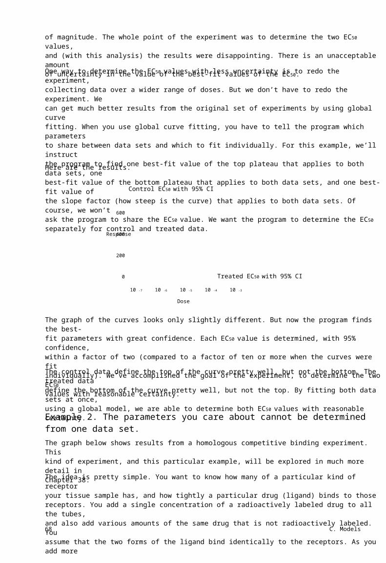
of magnitude. The whole point of the experiment was to determine the two EC50 values,and (with this analysis) the results were disappointing. There is an unacceptable amountof uncertainty in the value of the best-fit values of the EC50.

One way to determine the EC50 values with less uncertainty is to redo the experiment,collecting data over a wider range of doses. But we don’t have to redo the experiment. Wecan get much better results from the original set of experiments by using global curvefitting. When you use global curve fitting, you have to tell the program which parametersto share between data sets and which to fit individually. For this example, we’ll instructthe program to find one best-fit value of the top plateau that applies to both data sets, onebest-fit value of the bottom plateau that applies to both data sets, and one best-fit value ofthe slope factor (how steep is the curve) that applies to both data sets. Of course, we won’task the program to share the EC50 value. We want the program to determine the EC50separately for control and treated data.


Control EC50 with 95% CI

600

Response400

200

0

10 -7 10 -6 10 -5 10 -4

Treated EC50 with 95% CI

10 -3

Dose

The graph of the curves looks only slightly different. But now the program finds the best-fit parameters with great confidence. Each EC50 value is determined, with 95% confidence,within a factor of two (compared to a factor of ten or more when the curves were fitindividually). We’ve accomplished the goal of the experiment, to determine the two EC50values with reasonable certainty.

The control data define the top of the curve pretty well, but not the bottom. The treated datadefine the bottom of the curve pretty well, but not the top. By fitting both data sets at once,using a global model, we are able to determine both EC50 values with reasonable certainty.

Example 2. The parameters you care about cannot be determinedfrom one data set.The graph below shows results from a homologous competitive binding experiment. Thiskind of experiment, and this particular example, will be explored in much more detail inChapter 38.

The idea is pretty simple. You want to know how many of a particular kind of receptoryour tissue sample has, and how tightly a particular drug (ligand) binds to thosereceptors. You add a single concentration of a radioactively labeled drug to all the tubes,and also add various amounts of the same drug that is not radioactively labeled. Youassume that the two forms of the ligand bind identically to the receptors. As you add more

68 C. Models

of the unlabeled ligand, it binds to the receptors so less of the radioactive ligand binds. Soyou see downhill binding curves.

If you do such an experiment with a single concentration of radioactively labeled drug, theresults are not usually acceptable. You get a nice looking curve, but the confidenceintervals for both parameters you want to know (how many receptors and how tightly theybind) are very wide. You get almost the same results when you have lots of receptors thatbind your drug weakly or a few receptors that bind your drug tightly. Given theunavoidable experimental error, any one experiment simply gives ambiguous results.

If you use two different concentrations of labeled drug, as we did in our sampleexperiment, the situation is quite different. If you fit each of the two experimentsindividually, the results are unacceptable. The confidence intervals are extremely wide.But fit the two curves globally, telling the program to fit one value for receptor numberand one value for receptor affinity that applies to both data sets, and now the results arequite acceptable.

2500

2000 1 nMTotal Binding (DPM)

Best-fit valuesLOGKDBMAX

-8.92530791500

1000

500

0-12 -11 -10 -9 -8 -7 -6 -5

0.3 nM95% confidence intervals

LOGKDBMAX

-9.347 to -8.5041296 to 4862

Log [Cold]

Assumptions of global modelsWhen you fit a global model to a family of data sets, you are asking the program to findvalues of the parameters that minimize the grand sum-of-squares for all data sets. Thismakes sense only when:

• All data sets are expressed in same units. If different data sets wereexpressed in different units, you could give different data sets differentweights just by expressing the values in different units. For example,imagine what happens if you change one data set from expressing weight ingrams to expressing weight in milligrams. All the values are now increased bya factor of 1000, and the sum-of-squares for that data set is increased by afactor of one million (10002). Compared to other data sets, expressed indifferent units, this data set now has a much greater impact on the fit.

Tip: If you really want to do global fit to data sets using different units, firstnormalize the data so they are comparable.

• The scatter is the same for each data set. At each X value, for each data set,the scatter should be the same (unweighted fit) or should vary predictablywith Y (and be accounted for by weighting). If one data set has very littlescatter and another has lots of scatter, global fitting would not make sense.

6911. Global models

How to specify a global modelThe graph below shows an example of fitting a global model to data. We shared the top,bottom, and Hill slope and fit separate values for the LogEC50.

750

Response500

ControlTreated

250

0-8 -7 -6 -5 -4 -3 -2

log(Dose)

With Prism, you enter the data sets in side-by-side columns.

For this example, the built-in dose-response curve (variable slope) model is appropriate.

Y=Bottom + (Top-Bottom)/(1+10^((LogEC50-X)*HillSlope))

With Prism, use the Constraints tab of the nonlinear regression dialog to specify whichparameters to share. For this example, we share Bottom, Top and HillSlope, but notLogEC50. If you share any parameter or parameters, Prism uses global curve fitting.

Nonlinear regression fit five best-fit values: Bottom, Top, HillSlope, LogEC50 for controland LogEC50 for treated.

Parameter Best-fit value SE 95% CIBottom

Top

HillSlope

LogEC50 (control)

LogEC50 (treated)

110.0

578.6

0.7264

-5.618

-3.883

27.86

34.26

0.1857

0.07584

0.1767

38.33 to 181.6

490.6 to 666.7

0.2491 to 1.204

-5.813 to -5.423

-4.338 to -3.429

70 C. Models

The sum-of-squares is 5957 with 5 degrees of freedom (ten data points minus fiveparameters).

If you use a nonlinear regression program other than Prism, you’ll need to read itsdocumentation carefully to learn how to set up a global model. Most likely, you’ll need toenter the data with a grouping variable:

log(Dose)-7-6-5-4-3-7-6-5-4-3

Response165284442530573124 87195288536

Group1111122222

Enter the model, using IF-THEN statements to define a different logEC50 for each group.For our example, the first line of the equation could look something like this:

If (Group = 1) {LogEC50=LogEC50C} Else {LogEC50=LogEC50T}

Or this:

LogEC50 = IF(Group=1, LogEC50C, LogEC50T)

In those equivalent equations, we define the intermediate variable LogEC50 to equaleither the parameter LogEC50C (control) or logEC50T (treated) depending on the valueof Group. The rest of the equation (not shown) would then define Y as a function ofLogEC50.

Each program has its own way of dealing with IF-THEN relationships, but you probablywon’t find it hard to adapt the equations shown above.

11. Global models 71

12. Compartmental models and defining amodel with a differential equation

What is a compartmental model? What is a differential equation?Let’s create a pharmacokinetic model that explains how the concentration of a drug inblood plasma declines over time. You inject a bolus of drug, and measure plasma druglevels at various times thereafter. The drug is metabolized by a liver enzyme that is farfrom fully saturated. In this situation, the rate of drug metabolism is proportional to theconcentration of drug in the plasma. This is called first-order kinetics. When the plasmaconcentration is cut in half, so is the rate of drug metabolism.

This model can be shown as this compartmental diagram:

Plasma

Clearance (L/hr)VD

Metabolism

In this model, there is only one compartment labeled "plasma". In fact, this compartmentmay be larger than the plasma volume. It will include all other spaces that mix rapidlywith the plasma. The volume of distribution, VD, is the volume of this entirecompartment. In other words, it is the volume of blood plasma (liters) it would take tohold all the drug in the body if it were equally distributed. Clearance (in L/hr) is thevolume of blood plasma totally cleared of drug per minute.

Drawing a compartmental diagram helps clarify what is going on. From the diagram(some think of it as a map), you can easily create differential equations. A differentialequation defines how one variable changes as another variable changes.

In this case, we measure the concentration in the plasma, abbreviated Cplasma . Drug ismetabolized by a rate equal to the Clearance (liters/hour) times the concentration in theplasma (mg/liter). The product of clearance times concentration gives the rate of drugmetabolism in mg/hr. Divide by the volume of the plasma compartment (VD, in liters) tocompute the change in the concentration in the plasma.

Written as a differential equation, our model is:

dC plasma

dt=- Clearance

⋅ Cplasma

VD

Since we measure the concentration in the plasma, we call this Y. So the equation isequivalent to this equation and graph.

72 C. Models

dYClearance =-⋅YdtVD

Rate of change in plasma concentration (dY/dt)

Plasma Concentration

Your goal is to fit a curve to the data to learn the volume of distribution and clearance ofthe drug.

Integrating a differential equationUsing calculus, you (or someone you delegate this job to) can integrate the equation toform a standard model that defines Y as a function of t:

Yt =Y0 ⋅ e - Clearance ⋅t V D =Y0 ⋅ exp(-Clearance ⋅ t/VD )

At time zero, the concentration of drug (Y0) equals the dose you injected (D in mg) dividedby the volume of distribution (V0 in mL). So the equation can be rewritten like this:

D - VD ⋅t ⋅eYt = VD

C

Concentration of drug

Time

At any time t, the Y value (drug concentration) can be computed from the clearance, thevolume of distribution, and the time t. Set the dose to a constant, and use nonlinearregression to fit data to find the best-fit value of clearance and volume of distribution.

Note: With most nonlinear regression programs (including Prism), you’ll needto rewrite the model so the independent variable (time) is X rather than t.

12. Compartmental models and defining a model with a differential equation 73

The idea of numerical integrationIn the previous example, it was quite simple to integrate the differential equation toobtain an equation that defines Y (concentration) as a function of X (time). This is notalways possible.

Here are some data showing the metabolism of phenytoin over time following anintravenous injection of 300 mg.

Minutes mg/liter 7.88 7.10 6.79 5.27 4.52 3.43 1.97 1.01 0.23

10[Phenytoin] (mg/L)8

6

4

2

0

0 24 48 72 96

0 6 12 24 36 48 72 96144

120 144

Hours

Phenytoin saturates a large fraction of the enzyme that metabolizes it. This means that therate of metabolism is not proportional to drug concentration. The graph below comparesthe first-order model discussed in the previous section with the nonlinear (Michaelis-Menten) model appropriate for phenytoin metabolism. At very low drug concentrations,the two models are indistinguishable. But at higher drug concentrations, the two divergeconsiderably.

First-orderRate of drug metabolism (-dY/dt)

Vmax

Michaelis-Menten

KM Drug concentration

The rate of drug metabolism as a function of drug concentration follows the Michaelis-Menten relationship according to the equation below. Vmax is the maximum velocity of theenzyme (in mg/hr), when extrapolated to very high concentrations of drug that saturatethe enzyme. This is not related to VD , the volume of distribution in mL. The use of the

74 C. Models

variable “V” is a coincidence and Vmax and VD are not even measured in the same units. Kmis the concentration of phenytoin (in mg/liter) where drug metabolism is half-maximal.

Vmax ⋅ YdY =-dtVD (Km+Y)

This differential equation appears to be only slightly more complicated than the one in theprevious section. Instead of one parameter for drug clearance, we have two parameters(Vmax and Km ) that quantify the enzyme that degrades the drug. But this differentialequation is fundamentally different than the previous one. This differential equationcannot be integrated to form an equation that defines Y as a function of time, Vmax, VD, andKm. We think that it is simply impossible to integrate, no matter how adept you are atwrangling differential equations. It certainly is difficult.

Without an equation, how can we fit the model to data to find best-fit values of Vmax, VDand Km? Actually, we don’t need an equation. What we need is a computer procedure thatcalculates Y as a function of time, Vmax, VD and Km. We can do this without calculus bydoing brute force calculations. The idea is quite simple, and is best understood by anexample.

Based on previous literature, here are some initial parameters we can use when fitting thecurve. We found the parameters in a textbook of pharmacology. The parameters weretabulated as per kg, and we multiplied by 65 kg to get the values shown here.

Parameter Initial value CommentVD

Vmax

Km

Dose

42 liter

16 mg/hr

5.7 mg/liter

300 mg

Volume of distribution. Parameter to be fit.

Maximal elimination rate when enzyme is fully saturated.Parameter to be fit.

Drug concentration that half saturates themetabolizing enzyme. Parameter to be fit.

Dose injected intravenously at time zero. Experimentalconstant.

Beginning from these initial values, we want to use nonlinear regression to find best-fitvalues for Vd, Vmax and Km.

We can calculate the drug concentration (Y value) we expect to see at time=0. At timezero, the concentration of drug (Y0) equals the dose you injected (D in mg) divided by thevolume of distribution (V0 in mL), and so is 7.14 mg/liter. The graph above shows that theactual concentration of drug at time zero was a bit higher than that. Not a problem. Thevalues shown in the table above are just initial values. We’ll use nonlinear regression toget the best-fit values.

Let’s figure out the drug concentration an instant later. The trick is to pick a time intervalthat is small enough so drug concentration changes just a small amount, so the value Y onthe right side of the equation can be treated as a constant. To make the calculations easierto follow, we’ll start with a time interval of 0.25 hr. (Later we’ll switch to a smallerinterval.)


What is the value of Y at t=0.25 hr? We can rewrite the previous equation to substitute ∆t(a value we chose to equal o.25 hr) for dt and and ∆Y for dY (dY is a mathematical ideal;∆Y is an actual value).

Vmax ⋅ Y∆Y ≈-∆tVD (Km+Y)

Now rearrange to compute the change in Y.

∆Y ≈ - Vmax ⋅ Y ⋅ ∆tVD (Km+Y)

We have values for all the variables on the right side of the equation, so we can calculatethe value of ∆Y, which will be negative (the drug concentration is going down over time).For this example, ∆Y equals -0.0530 mg/liter. Add this negative value to the drugconcentration at time 0 (7.14 mg/liter), and you’ve computed the concentration at time 1minute (7.090 mg/liter). Plug this new value of Y into the right of the equation (the othervariables don’t change) and calculate a new value of ∆Y for the change from time 0.25 hrto 0.50 hr. This time, ∆Y= -0.0528 mg/liter. Add this negative value to the concentrationat time 0.25 hr and you’ve computed the concentration at time 0.50 hr, which is 7.090mg/liter.

Repeat this procedure many times (with a program or spreadsheet), and you can graphpredicted drug concentration (Y) as a function of time (X). This procedure, which doesn’trequire any calculus, is called numerical integration.

10[Phenytoin] (mg/L) 8

6

4

2

0

0 24 48 72 96 120 144

Hours

The curve doesn’t go through our data. But that’s ok. The curve was generated from somepublished (average) values. Now we want to fit the model to our data to find the kineticparameters in this individual.

The only real trick to numerical integration is choosing a value for ∆t. The method will beinaccurate if ∆t is too large. In fact, we would have gotten slightly different (and moreaccurate) values if we had used a smaller ∆t in our example. If ∆t is small, the calculationswill take longer. If ∆t is really tiny, the calculations may lose accuracy. For details aboutchoosing ∆t and numerical integration, read Numerical Recipes in C.

To improve accuracy, we decreased a ∆t to 0.01 hour, and fit the model to the data. Hereare the best-fit values of the parameters, along with a graph of the resulting curve.

76 C. Models

ParameterVd

Vmax

Km

Best-fit value38.2

6.663

4.801

Unitsliter

mg/hr

mg/liter

10[Phenytoin] (mg/L) 8

6

4

2

0

0 24 48 72 96 120 144

Hours

If your program lets you enter a model as a differential equation, you’ll also need to definethe Y value at time zero (for this example, you want to enter an equation that defines Y attime zero from the parameters). After that, curve fitting works as usual and there isnothing special about interpreting the results. Because numerical integration requires lotsof calculations, and these need to be repeated over and over as nonlinear regressionprogresses, fitting a model defined by a differential equation takes longer than fitting amodel defined by an ordinary equation.

Note: Few nonlinear programs will let you express a model as a differentialequation. GraphPad Prism 4.0 cannot fit models expressed this way, althoughthis is a feature we are likely to add to a future version.

More complicated compartmental modelsHere is an example of a more complicated compartmental model. It models the plasmaconcentration of estrogen.


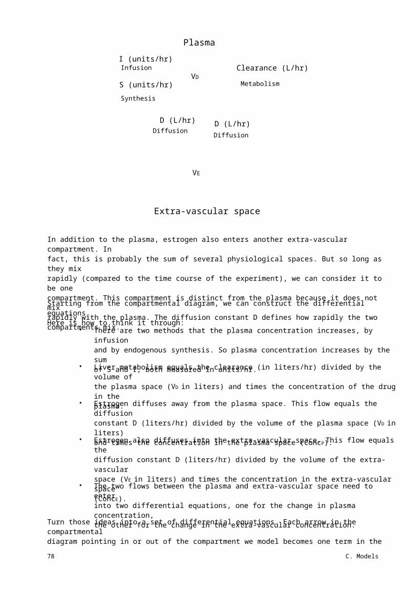
PlasmaI (units/hr)Infusion

S (units/hr)Synthesis

VDClearance (L/hr)

Metabolism

D (L/hr)Diffusion

D (L/hr)Diffusion

VE

Extra-vascular space

In addition to the plasma, estrogen also enters another extra-vascular compartment. Infact, this is probably the sum of several physiological spaces. But so long as they mixrapidly (compared to the time course of the experiment), we can consider it to be onecompartment. This compartment is distinct from the plasma because it does not mixrapidly with the plasma. The diffusion constant D defines how rapidly the twocompartments mix.

Starting from the compartmental diagram, we can construct the differential equations.Here is how to think it through:

• There are two methods that the plasma concentration increases, by infusionand by endogenous synthesis. So plasma concentration increases by the sumof S and I, both measured in units/hr.

Liver metabolism equals the clearance (in liters/hr) divided by the volume ofthe plasma space (VD in liters) and times the concentration of the drug in theplasma.

Estrogen diffuses away from the plasma space. This flow equals the diffusionconstant D (liters/hr) divided by the volume of the plasma space (VD in liters)and times the concentration in the plasma space (ConcP).

Estrogen also diffuses into the extra-vascular space. This flow equals thediffusion constant D (liters/hr) divided by the volume of the extra-vascularspace (VE in liters) and times the concentration in the extra-vascular space(ConcE).

The two flows between the plasma and extra-vascular space need to enterinto two differential equations, one for the change in plasma concentration,the other for the change in the extra-vascular concentration.

•

•

•

•

Turn those ideas into a set of differential equations. Each arrow in the compartmentaldiagram pointing in or out of the compartment we model becomes one term in the

78 C. Models

differential equation. The change in concentration equals the sum of all flows into thatcompartment minus the sum of all flows leaving the compartment.

dConc plasma

dt=I+S-

Clearance ⋅ ConcPlasma D ⋅ Conc E D ⋅ Conc Plasma

+- VDVEVD

dConc E D ⋅ Conc Plasma D ⋅ Conc E

=- dtVDVE

Note: Some programs (not from GraphPad) let you enter the model as acompartmental model. You draw boxes and arrows in the program, and itgenerates the differential equations automatically.

Now you can use the model to simulate data. Or use nonlinear regression (with anappropriate program, not from GraphPad) to fit experimental data and find best-fitparameters.


D. How nonlinear regression works

13. Modeling experimental error

Why the distribution of experimental error matters when fittingcurvesThe goal of regression is to find best-fit values for the parameters of the model (e.g., slopeand intercept for linear regression, other parameters, such as rate constants, for nonlinearregression). More precisely, the goal is to find values for the parameters that are mostlikely to be correct. It turns out that you can’t decide which parameter values are mostlikely to be correct without making an assumption about how the data are scatteredaround the line or curve.

Note: Statisticians refer to the scatter of points around the line or curve as“error”. This is a different use of the word than is used ordinarily. In statistics,the word “error” simply refers to deviation from the average. The deviation isusually assumed to be due to biological variability or experimental imprecision,rather than a mistake (the nontechnical meaning of “error”).

Origin of the Gaussian distributionMost linear and nonlinear regression assumes that the scatter follows a Gaussian (alsocalled a “normal”) distribution. This section explains what the Gaussian distribution is,and why it is so central to statistics.

Imagine a very simple “experiment”. You pipette some water, and weigh it. Your pipette issupposed to deliver 10 mL of water, but in fact delivers randomly between 9.5 and 10.5mL. If you pipette one thousand times, and create a frequency distribution histogram ofthe results, it will look like something like this.

75Number of experiments

50

25

09.5 10.0 10.5

Weight in grams

80 D. How nonlinear regression works

The average weight is 10 grams, the weight of 10 mL of water (at least on Earth). Thedistribution is flat, with random variation.

Now let’s make the experiment slightly more complicated. We pipette two aliquots of 10mL and weigh the result. On average, the weight will now be 20 grams. But the errors willcancel out much of the time. Values close to 20 grams will be more likely than values farfrom 20 grams. Here is the result of 1000 such (simulated) experiments.

Number of experiments

100

50

019.0 19.5 20.0 20.5 21.0

Weight in grams

Each pipetting step has a flat random error. Add up the result of two pipetting steps, andthe distribution is not flat. For example, you’ll get weights near 21 grams only if bothpipetting steps err substantially in the same direction, and that will happen rarely. Incontrast, you can get a weight of 20 grams in lots of ways, so this happens morecommonly.

Now let’s make the experiment more realistic with ten steps. Here are the results of 15000simulated experiments. Each result is the sum of ten steps.

1500Number of experiments

1000

500

0 97 98 99 100 101 102 103

Weight in grams

You’ll recognize this distribution. It is the Gaussian bell-shaped distribution, which iscentral to much of statistics.

If your experimental scatter has numerous sources that are additive and of nearly equalweight, you expect the scatter of replicate values to approximate a Gaussian distribution.This also means that you’ll expect the deviations of points around the curve to follow aGaussian distribution.

13. Modeling experimental error 81

The Gaussian distribution is a mathematical ideal, which extends from negative infinity topositive infinity. If the weights in the example above really followed a Gaussiandistribution exactly, there would be some chance (albeit very small) of having a negativeweight. Since weights can’t be negative, the distribution cannot be exactly Gaussian. But itis close enough to Gaussian to make it ok to use statistical methods (like regression) thatassume a Gaussian distribution. Few biological distributions, if any, completely follow theGaussian distribution, but many are close enough.

Tip: The Gaussian distribution is also called a Normal distribution. Don’tconfuse this use of the word “normal” with its other meanings of “ordinary”,“common”, or “disease free”.

From Gaussian distributions to minimizing sums-of-squaresGiven the assumption that scatter follows a Gaussian distribution, how do we decidewhich parameter values are most likely to be correct?

Mathematical statisticians approach this problem using a method called maximumlikelihood. Start with a data set, a model, and an assumption about how the data arescattered around the model. Given a model, a set of parameters, and an assumption aboutscatter, it is possible to calculate the likelihood of generating your data. Some sets ofparameters are very unlikely to have generated your data, because the curve thoseparameters define is far from your data. Other sets of parameters (those that define acurve near your data) are more likely. The maximum likelihood method finds the set ofparameter values that are most likely to have generated your data.

The maximum likelihood method can be used with almost any assumption about thedistribution of the data. However, standard nonlinear (and linear) regression is almostalways based on the assumption that the scatter follows a Gaussian distribution. Giventhis specific assumption, it can be proven that you can find the most likely values of theparameters by minimizing the sum of the squares of the vertical distances (“residuals”) ofthe points from the line or curve.

Unless you have studied statistics in depth, it isn't obvious how the assumption of aGaussian distribution of residuals (distances of points from curve) leads to the rule thatyou find the most likely parameters by minimizing the sum-of-squares. But the two arelinked. If you make some other assumption about the scatter of replicates, then you’llneed to use a different rule (not least-squares) to find the values of the parameters thatare most likely to be correct.

If you want to understand more about maximum likelihood methods, and how the least-squares rule was derived, read section 15.1 of Numerical Recipes in C, which you can findonline at www.nr.com.

Here is an intuitive way to get a sense of why minimizing the sum of the squares of thedistances makes sense. Two points from a set of data scattered randomly according to aGaussian distribution are far more likely to have two medium size deviations (say 5 unitseach) than to have one small deviation (1 unit) and one large (9 units). A procedure thatminimized the sum of the absolute value of the distances would have no preference over aline (or curve) that was 5 units away from two points and a line (or curve) that was 1 unitaway from one point and 9 units from another. The sum of the distances (more precisely,the sum of the absolute value of the distances) is 10 units in each case. If, instead, youchoose a procedure that minimizes the sum of the squares of the distances, then a fit thatproduces a line 5 units away from two points (sum-of-squares = 50) is a much better fit


than one that produces a line 1 unit away from one point and 9 units away from another(sum-of-squares = 82). If the scatter is Gaussian (or nearly so), the line determined byminimizing the sum-of-squares is most likely to be correct.

Regression based on nongaussian scatterThe assumption of a Gaussian distribution is just that, an assumption. It is a usefulassumption, because many kinds of data are scattered according to a Gaussiandistribution (at least approximately) and because the mathematical methods based on theGaussian distribution work so well.

Not all data are scattered according to a Gaussian distribution, however. Some kinds ofdata, for instance, follow a Poisson distribution, and regression methods have beendeveloped that assume such a distribution for experimental errors.

It is also possible to assume a very wide distribution, such as the Lorentzian distribution(also called the Cauchy distribution), shown below. This distribution is much wider than aGaussian distribution.

Gaussian

Probability Density

Lorentzian

-5 -4 -3 -2 -1 0 1 2 3 4 5Distance of point from curve

If you fit data to a model assuming this distribution, outliers (points far from the curve)will have less influence. The Lorentzian distribution is the same as a t distribution with 1degree of freedom. The Gaussian distribution is the same as a t distribution with manydegrees of freedom. By varying the number of degrees of freedom, the t distributiongradually changes from having a wide distribution to a compact one.

GraphPad note: GraphPad Software, in collaboration with AISN Software, isworking hard to develop a version of Prism that can fit assuming a Lorentziandistribution. Curve fitting done this way is much more robust to outliers. Fordetails, go to www.graphpad.com and search for “robust”.

13. Modeling experimental error 83

14. Unequal weighting of data points

Standard weightingAs outlined in the previous chapter, regression is most often done by minimizing the sum-of-squares of the vertical distances of the data from the line or curve. Points farther fromthe curve contribute more to the sum-of-squares. Points close to the curve contributelittle. This makes sense, when you expect experimental scatter to be the same, on average,in all parts of the curve.

The graph below is an example of data collected with twenty replicates at each drug dose.The scatter is Gaussian and the standard deviation among the replicates is about the sameat each dose. With data like these, it makes sense to minimize the sum-of-squares of theabsolute distances between the points and the curve.

3000

Response2000

1000

0

-9 -8 -7 -6 -5 -4 -3log(dose, M)

Note: This example purposely exaggerates the scatter to make the exampleeasier to follow.

Relative weighting (weighting by 1/Y2)In many experimental situations, you expect the average distance (or rather the averageabsolute value of the distance) of the points from the curve to be higher when Y is higher.The relative distance (distance divided by Y), however, remains about the same all the wayalong the curve.

Here is another example dose-response curve. At each dose, twenty replicate values areplotted. The distribution of replicates is Gaussian, but the standard deviation varies. It is


small at the left side (bottom) of the graph and large at the right side (top). While thestandard deviation of the error is not consistent along the graph, the relative variability isconsistent. In fact, these data were simulated by selecting random numbers from aGaussian distribution with a standard deviation equal to 20% of the mean value.

3000

Response2000

1000

0-9 -8 -7 -6 -5 -4 -3

log(dose, M)

In this common situation, minimizing the sum-of-squares of the absolute verticaldistances would be inappropriate. If you did that, points with high Y values would tend tohave large deviations from the curve and so would have a large impact on the sum-of-squares value. In contrast, points with smaller Y values would have little influence. This isnot desirable – you want all the points to have about equal influence on the goodness-of-fit. To do this, minimize the sum of the square of the relative distances.

The relative distance of a data point from the curve is given by

YData -YCurve

YData

If you choose relative weighting, nonlinear regression minimizes the sum of squares ofrelative distances:

YData -YCurve ∑ YData

2

Relative weighting is often called weighting by 1/Y2. Rearranging the expression showswhy.

1∑ Y (Y2

DataData

-YCurve ) 2

14. Unequal weighting of data points 85

Note: Some programs weight by the square of the Y value of the curve (thepredicted Y value) rather than the Y value of the data points. This distinction(whether the denominator is the Y value of the data or curve) rarely will affectthe results very much.

Poisson weighting (weighting by 1/Y)Weighting by 1/Y is a compromise between minimizing the actual (absolute) distancesquared and minimizing the relative distance squared. One situation where 1/Y weightingis appropriate is when the Y values follow a Poisson distribution. This would be the casewhen Y values are radioactive counts and most of the scatter is due to counting error.With the Poisson distribution, the standard deviation among replicate values isapproximately equal to the square root of that mean. To fit a curve, therefore, youminimize the sum of squares of the distance between the data and the curve divided bythe square root of the value. In other words, nonlinear regression minimizes thisexpression:

YData -YCurve

∑ Y data

2

Rearrangement shows why it is sometimes called weighting by 1/Y.

1∑ Y (YData

Data-YCurve ) 2

Note: Weighting by 1/Y is one way to cope with data distributed according to aPoisson distribution, but a better way is to use a regression method that isbased upon an assumption of a Poisson regression. Look for a program that canperform “Poisson regression”.

Weighting by observed variabilityRelative and Poisson weighting assume that you know how the scatter varies as the Yvalues vary. Often you don’t know. It sounds appealing, therefore, to base the weightingon the observed variation among replicates. If you have collected triplicate values, whynot just base the weighting on the standard deviation of those values? Give points a highweight when the triplicates are tightly clustered with a small SD. Give points a low weight,when the triplicates are scattered with a large SD. In other words, minimize this quantity:

12 Y -Y

∑ DataSD Curve =∑ SD2 ( YData -YCurve )

Tip: We suggest that you rarely, if ever, use this method. Read this sectioncarefully before weighting by the inverse of the standard deviation. The methodsounds more useful than it is.

This method assumes that the mean of replicates with a large standard deviation is lessaccurate than the mean of replicates with a small standard deviation. This assumptionsounds sensible, but it is often not true. When you only have a few replicates, the standard


2

deviation will vary considerably just by chance. The figure below makes this point. Itshows fifteen sets of triplicate values. Each value was chosen from a Gaussian distributionwith a mean of 50 and a SD of 10. There is no difference between the fifteen data setsexcept for that due to random sampling. Compare the first (A) and last (O) data sets. TheSD of the last data set is three times that of the first data set. Yet the mean of last data setis closer to the true mean (known to be 50 since these data were simulated) than is themean of the first data set.

100

75

50

25

0A B C D E F G H I J K L M N O

With a small number of replicates, the observed scatter jumps all over the place just bychance. The mean of a set of replicates with a small SD is not necessarily more accuratethan the mean of a set of replicates with a larger SD. The small SD tells you that thereplicates are clustered near each other, but this may not be close to the true value.

You want to choose a weighting scheme to account for systematic differences in thepredicted amount of variability if you were to repeat the experiment many times. Youshould not choose weighting based on variability you happened to observe in one smallexperiment. That won’t be helpful. Therefore it only makes sense to weight by theobserved SD among replicates when you have lots (dozens) of replicates.

Error in both X and YConventional linear and nonlinear regression assume that all the uncertainty is in the Ydirection and that you know X precisely. A special kind of linear regression, called ModelII or Deming regression (see page 50) allows for the possibility that there is error in bothvariables. Some methods have also been developed to account for error in both X and Yvariables of nonlinear models, but these are not commonly used, and are beyond thescope of this book.

Weighting for unequal number of replicatesIn most experiments, you collect replicate Y values at every value of X. How you analyzeyour replicates depends on your experimental design.

Independent replicatesIn most experiments, it is fair to consider each replicate to be an independent data point.Each particular replicate is subject to random factors, which may increase or decrease its

14. Unequal weighting of data points 87

value. Each random factor affects individual replicates, and no random factor affects thereplicates as a group. In any kind of biochemical experiment, where each value comesfrom a test tube or plate well, the replicates are almost certain to be independent.

When your replicates are independent, you should treat each replicate as a separate point.With some programs, this means you’ll have to repeat your X values, as shown in the tableshown on the left below. With other programs (such as Prism) you can put your replicatesside by side, as shown on the table on the right below.

Dose1

1

1

2

2

2

3

3

3

Response3.4

2.9

3.1

4.5

5.1

4.7

5.9

6.2

6.3

Dose

X1

2

3

Y13.4

4.5

5.9

Response

Y22.9

5.1

6.2

Y33.1

4.7

6.3

Every replicate is treated by the nonlinear regression program as a separate data point. Ifthere are four replicates at one X value and two at another, the four replicates willautomatically get twice the weight, since the program considers them to be four separatedata points.

An alternative is to average the replicate Y values and treat the mean as a single datapoint. If you have different number of replicates for different values, then you definitelyshould not average the replicates and fit to the means. The results will be wrong. If you dohave the same number of replicates for every point (e.g., no missing values), fitting tomeans or fitting to individual replicates will give you the same best-fit values of theparameters and thus exactly the same best-fit curve. But the standard errors andconfidence intervals won’t be the same. Fitting to the means, rather than the replicates,can make the standard errors larger or smaller (the confidence intervals wider ornarrower), depending on the data set.

Tip: If your replicates are independent, treat each one as a separate data point.Don’t try to fit the averages.

Replicates that are not independentIn some experimental situations, the replicates are not independent. Random factors canaffect all the replicates at once. Two examples:

• You performed a binding experiment with a single tube at eachconcentration, but measured the radioactivity in each tube three times.Those three values are not independent. Any experimental error whileconducting the experiment would affect all the replicates.

D. How nonlinear regression works88

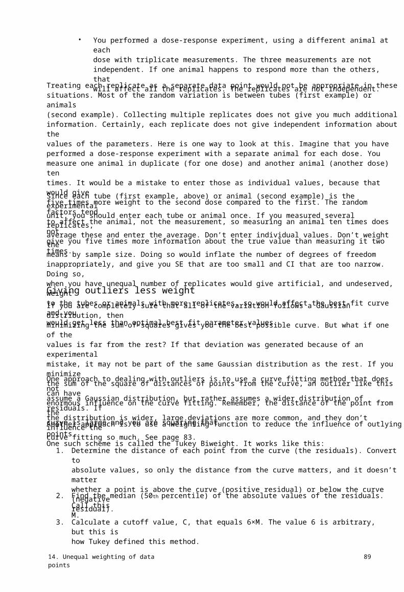
• You performed a dose-response experiment, using a different animal at eachdose with triplicate measurements. The three measurements are notindependent. If one animal happens to respond more than the others, thatwill affect all the replicates. The replicates are not independent.

Treating each replicate as a separate data point would not be appropriate in thesesituations. Most of the random variation is between tubes (first example) or animals(second example). Collecting multiple replicates does not give you much additionalinformation. Certainly, each replicate does not give independent information about thevalues of the parameters. Here is one way to look at this. Imagine that you haveperformed a dose-response experiment with a separate animal for each dose. Youmeasure one animal in duplicate (for one dose) and another animal (another dose) tentimes. It would be a mistake to enter those as individual values, because that would givefive times more weight to the second dose compared to the first. The random factors tendto affect the animal, not the measurement, so measuring an animal ten times does notgive you five times more information about the true value than measuring it two times.

Since each tube (first example, above) or animal (second example) is the experimentalunit, you should enter each tube or animal once. If you measured several replicates,average these and enter the average. Don’t enter individual values. Don’t weight themeans by sample size. Doing so would inflate the number of degrees of freedominappropriately, and give you SE that are too small and CI that are too narrow. Doing so,when you have unequal number of replicates would give artificial, and undeserved, weightto the tubes or animals with more replicates, so would affect the best-fit curve and youwould get less than optimal best fit parameter values.

Giving outliers less weightIf you are completely sure that all of the variation follows a Gaussian distribution, thenminimizing the sum-of-squares gives you the best possible curve. But what if one of thevalues is far from the rest? If that deviation was generated because of an experimentalmistake, it may not be part of the same Gaussian distribution as the rest. If you minimizethe sum of the square of distances of points from the curve, an outlier like this can haveenormous influence on the curve fitting. Remember, the distance of the point from thecurve is large and you are squaring that.

One approach to dealing with outliers is to use a curve fitting method that does notassume a Gaussian distribution, but rather assumes a wider distribution of residuals. Ifthe distribution is wider, large deviations are more common, and they don’t influence thecurve fitting so much. See page 83.

Another approach is to use a weighting function to reduce the influence of outlying points.One such scheme is called the Tukey Biweight. It works like this:

1. Determine the distance of each point from the curve (the residuals). Convert toabsolute values, so only the distance from the curve matters, and it doesn’t matterwhether a point is above the curve (positive residual) or below the curve (negativeresidual).

Find the median (50th percentile) of the absolute values of the residuals. Call thisM.

Calculate a cutoff value, C, that equals 6×M. The value 6 is arbitrary, but this ishow Tukey defined this method.

89

2.

3.

14. Unequal weighting of data points

4. Give any point whose residual (distance from the curve) exceeds C a weight of zero.These points are so far from the curve that they can’t possibly be right. By givingthem a weight of zero, the points are ignored completely.

Give the other points a weight determined by the equation below, where R is theabsolute value of the distance of that point from the curve, and C was defined instep 4 above. From this equation, you can see why this method is termed abisquare method.

5.

R 2 Weight= 1- C

6.

2

When computing the weighted sum-of-squares, the contribution of each point isthe distance of the point from the curve (R) squared times the weighting factorabove. In other words, after ignoring points whose distance from the curve exceedsC, this method asks the curve fitting program to minimize:

R 2 2

∑ R 1- C

7.

2

With each iteration of nonlinear regression, recompute the weights. As the curvefitting progresses, the curve will change, so the distribution of residuals will changeas will the assignment of bisquare weights.

The graph below shows the contribution of a point to this adjusted sum-of-squares as afunction of its distance from the curve. Half the points, by definition, are closer to thecurve than the median value. For these points (R<1), the least-squares and Tukey biweightmethods treat the points about the same. As the points get farther from the curve, up toR=3 (three times the median distance) their influence still increases with the Tukeybiweight method, but not as much as they’d increase with standard least-squaresregression. Points that are between 3 and 6 times the median distance from the curve stillcontribute to the curve fitting, but their influence decreases as they get farther from thecurve. Points that are more than six times the median distance are ignored completely bythe bisquare method.

Influence on curve fitting Least-squares

Tukey Biweight

0 1 2 3 4 5 6 7 Distance from curve, R(Multiple of median deviation)

GraphPad note: No GraphPad program performs regression with the Tukeybiweight method.

15. How nonlinear regression minimizes thesum-of-squares

Nonlinear regression requires an iterative approachNonlinear regression is more complicated than linear regression. You can’t compute thebest-fit values of the parameters directly from the X and Y values of the data points.Instead, nonlinear regression requires an iterative approach.

You won't be able to understand the mathematical details of nonlinear regression unlessyou first master matrix algebra. But the basic idea is pretty easy to understand. Everynonlinear regression method follows these steps:

1.

2.

3.

4.

5.

6.

7.

Start with an initial estimated value for each parameter in the equation.

Generate the curve defined by the initial values.

Calculate the sum-of-squares (the sum of the squares of the vertical distances ofthe points from the curve).

Adjust the parameters to make the curve come closer to the data points. There areseveral algorithms for adjusting the variables, as explained in the next section.

Adjust the parameters again so that the curve comes even closer to the points.Repeat.

Stop the calculations when the adjustments make virtually no difference in thesum-of-squares.

Report the best-fit results. The precise values you obtain will depend in part on theinitial values chosen in step 1 and the stopping criteria of step 6. This means thatdifferent programs will not always give exactly the same results.

Step 4 is the only difficult one. Most nonlinear regression programs use the method ofMarquardt and Levenberg, which blends two other methods, the method of steepestdescent and the method of Gauss-Newton. The next section explains how these methodswork.

How the nonlinear regression method works

Fitting one parameterThe example below shows a signal that decreases over time. The results are normalized torun from 100% at time zero to 0% at infinite times.

15. How nonlinear regression minimizes the sum-of-squares 91

Minutes 0.5 1.0 1.5 2.0 2.5 3.0 3.5 4.0 4.5 5.0 5.5 6.0

Percent 83.9 72.9 56.5 39.4 33.3 38.1 25.0 23.8 14.3 12.0 19.0 6.0

100%

Signal50%

0%0 1 2 3 4 5 6 7

Minutes

We wish to fit this to an exponential decay model, fixing the top to 100 and the bottomplateau to 0, leaving only one parameter, the rate constant (k), to fit to this model:

Y=100 ⋅ e -k ⋅XSince we are only finding the best-fit value of one parameter, we can do so in a brute-forcemanner. By looking at the data, and knowing the meaning of the rate constant, we can bequite sure the best-fit value is between 0.2 and 0.7. From the goals of the experiment, wecan say that we only need to know the best-fit value to two decimal places. So there areonly 50 possible values of k (0.20, 0.21, 0.22, …, 0.69, 0.70). For each of these values,construct a curve, and compute the sum-of-squares of the distances of the points from thecurve. Below is a graph of sum-of-squares as a function of k. Note that this graph wasconstructed specifically for this example. With different data, the graph would lookdifferent.

3000

Sum-of-squares2000

1000

0

0.2 0.3 0.4 0.5 0.6 0.7Possible value of k

The sum-of-squares was smallest when k equals 0.39. That is our best-fit value. We'redone.

Since we are only fitting one parameter, that brute force method worked fine. But if you fitseveral parameters, the number of possible combinations of values becomes astronomical.We need a more efficient way to find the best-fit values.

Nonlinear regression begins with an initial value of k that you give the program (or theprogram generates from the range of the X values). For this example, the initial value is


0.3. Mathematicians have developed several methods to move from the initial values tofind the values of the parameters that minimize the sum of squares.

The method of steepest descent follows a very simple strategy. You start with theinitial estimate of the parameters (k in this example). This initial value generates a curve,and you can compute the sum-of-squares of the points from this curve. This correspondsto a point on the graph shown above. From that point, figure out which way is downhill. Isthe value of k too high or too low? Our initial value of 0.3 is too low. So we increase the ka small amount. The step size is somewhat arbitrary. We'll take a step of 0.1, to reach thevalue of k=0.4. Generate the curve defined by this value of k, and compute the sum-of-squares. Indeed it is lower. Repeat many times. Each step will usually reduce the sum-of-squares. If the sum-of-squares goes up instead, the step must have been so large that youwent past the bottom and back up the other side. This means your step size is too large, sogo back and take a smaller step. After repeating these steps many times, graduallydecreasing the step size, you'll reach the bottom. You’ll know you are on the bottom,because every step you take (every small change in the value of k), in either direction,leads up hill (increases the sum-of-squares)

The Gauss-Newton method is a bit harder to understand. As with the method ofsteepest descent, start at the spot defined by the initial estimated values. Then computehow much the sum-of-squares changes when you make a small change in the value of k.This tells you the steepness of the sum-of-squares curve at the point defined by the initialvalues. If the model really were linear, the sum-of-squares curve would have a regularshape. Knowing one point, and the steepness at that point completely defines that curve,and so defines its bottom. With a linear equation, you go from initial estimate values tobest-fit values in one step using the Gauss-Newton method. With nonlinear equations, thesum-of-squares curve has an irregular shape so the Gauss-Newton method won't find thebest-fit value in one step. But in most cases, the spot that the Gauss-Newton methodpredicts is the bottom of the surface is closer to the bottom. Starting from that spot, figureout the steepness again, and use the Gauss-Newton method to predict where the bottomof the valley is. Change the value of k again. After repeating many iterations, you willreach the bottom.

This method of steepest descent tends to work well for early iterations, but works slowlywhen it gets close to the best-fit values. In contrast, the Gauss-Newton method tends towork badly in early iterations, but works very well in later iterations (since the bottom ofthe sum-of-squares curve tends to approximate the standard shape, even for nonlinearmodels). The two methods are blended in the method of Marquardt (also called theLevenberg-Marquardt method). It uses the method of steepest descent in earlyiterations and then gradually switches to the Gauss-Newton approach. Mostcommercially-available computer programs use the Marquardt method for performingnonlinear regression.

Any of these methods finds that the best-fit value of k is 0.3874 min-1). Here is the best-fitcurve.


100%

k = 0.3874 min-1

Signal50%

0%0 1 2 3 4 5 6 7

Minutes

Two parametersHere are some data to be fit to a typical binding curve (rectangular hyperbola).

1500

Specific Binding(fmol/mg protein)1000

500

00 10 20 30 40 50 60 70

[Ligand] (nM)

You want to fit a model defining equilibrium binding. This equation has two parameters,Bmax and Kd.

Y=Bmax ⋅ XK d +X

How can you find the values of Bmax and Kd that fit the data best? You can generate aninfinite number of curves by varying Bmax and Kd. Each pair of Bmax and Kd valuesgenerates a curve, and you can compute the sum-of-squares to assess how well that curvefits the data. The following graph illustrates the situation.


106

sSum-of-square

105

Best fit

8

16001400

1200 41000

10

Bm ax

The X and Y axes correspond to two parameters to be fit by nonlinear regression (Bmax andKd in this example). Every pair of values for Kd and Bmax define a curve, and the Z-axisplots the sum-of-squares of the vertical distances of the data points from that curve. Notethat this graph was created specifically for the data set shown previously. The data are notgraphed. Instead the graph shows how those particular data fit curves defined by variousvalues of Bmax and Kd.

The goal of nonlinear regression is to find the values of Bmax and Kd that make the sum-of-squares as small as possible. In other words, the goal is to find the point on that surfacethat is lowest (has the smallest sum-of-squares). More simply, the goal is to find thebottom of the valley. The three methods described in the previous section all can be used,and find the bottom of the surface. Rather than adjust one parameter during eachiteration, both are adjusted at once, working our way down the surface to find its lowpoint.

More than two parametersIt was pretty easy to visualize the optimization of one parameter on a two-dimensionalgraph. And it wasn't too hard to visualize optimization of two parameters on a threedimensional graph. Once you have three or more parameters, it is not possible to visualizethe search for optimum parameter values graphically. But the sum-of-squares graphsshown in the previous two sections were just shown to explain the idea behind themethod. The method actually works via matrix algebra, and it works for any number ofparameters. Nonlinear regression can fit any number of parameters.

The Simplex methodWhile the Marquardt method is used most often, some programs use an alternativemethod called the Simplex method. While the Marquardt method starts with one set ofinitial estimated values (one for each parameter), the Simplex method requires K+1 sets ofinitial values, where K is the number of parameters you are fitting. The example shownabove fits two parameters, so the Simplex method requires three sets of initial values (onemore than the number of parameters). These three sets of initial values become three


K d

104 6

points on the 3D surface shown in the figure above. For each set of initial values, theSimplex method generates the curve and calculates the sum-of-squares. One set of initialvalues has the highest sum-of-squares (the worst fit). The Simplex method discards thatset of values and finds a new set that fits better (using a complicated set of rules). Thisprocess is repeated until the sets of parameters become indistinguishable. With twoparameters (as in our example), this can be visualized as a triangular amoeba crawlingdown the surface, gradually becoming smaller, until the points of the triangle are almostsuperimposed. The advantage of the Simplex method is that it can sometimes find a goodsolution in difficult situations where the other methods give up with an error message.The disadvantage, and it is a major one, is that the Simplex method does not compute astandard error or confidence interval for the parameters. You get best-fit values, but youdon’t know how precise they are.

Note: While the Simplex method does not automatically create confidenceintervals, it is possible to create confidence intervals using Monte Carlosimulations (Chapter 17) or via method comparison (see Chapter 18).

Independent scatterNonlinear regression, as usually implemented, assumes not only that the scatter isGaussian, but also that each data point has independent scatter. We’ll discuss themeaning of independence in terms of replicates on page 87. If X is time, it is alsoimportant that adjacent data points do not influence each other.

In the diagram below, the horizontal line is the ideal curve, which happens to behorizontal for this simplified example. The data point (circle) on the left is themeasurement at time 1. By chance, experimental error made that value fall below the idealcurve. If the measurements are entirely independent, as is assumed by linear andnonlinear regression, then the value at time 2 should not be affected by the value at time 1.This means that:

•

•

•

C is the most likely value.

D and B are equally likely.

A is quite unlikely.

D

Signal C

B

A

Time 1 Time 2

In some experimental systems, there is a carryover from one time point to the next. Inthese systems, the most likely value at time 2 is B, with A and C equally likely, and D veryunlikely. If your data are like this, standard linear and nonlinear regression are notappropriate. Extensions to nonlinear regression are being developed to handle thissituation (J. Celantano, personal communication, 2002).


E. Confidence intervals of the parameters

16. Asymptotic standard errors and confidenceintervals

Interpreting standard errors and confidence intervalsIn most situations, the whole point of regression is to find the best-fit values of theparameters. Your goal is to understand your system, or perhaps to look at how aparameter changes with a treatment. If this is your goal, then you will certainly care abouthow precisely you know the best-fit values of the parameters. It isn’t enough to know, forexample, that the best fit value of a rate constant is 0.10 min-1. Your conclusion will bevery crisp if the program tells you that you can be 95% sure the true rate constant liesbetween 0.09 and 0.11 min-1. On the other hand, you’ll know the results are pretty sloppyif the program tells you that you can be 95% sure the true rate constant lies between 0.0and 0.5 min-1. This tells you very little except that you need to redesign your experiment.Your entire interpretation of the results, and your decision on what to do in futureexperiments, depends on knowing the confidence intervals (or standard errors) of theparameters.

You can only interpret nonlinear regression results if the assumptions of nonlinearregression are true or at least not badly violated (see page 30). If you accept theseassumptions, the 95% CI is supposed to be an interval that has a 95% chance of containingthe true value of the parameter. More precisely, if you perform nonlinear regression manytimes (on different data sets) you expect the confidence interval to include the true value95% of the time, but to exclude the true value the other 5% of the time (but you won'tknow when this happens).

The standard errors reported by most nonlinear regression programs (including Prism)are “approximate” or “asymptotic”. Accordingly, the confidence intervals computed usingthese errors should also be considered approximate.

Does it matter that the confidence intervals are only approximately correct? That dependson how you want to use those intervals. In most cases, you’ll use the confidence intervalsto get a sense of whether your results are any good. If the confidence intervals are narrow,you know the parameters precisely. If the confidence intervals are very wide, you knowthat you have not determined the parameters very precisely. In that case, you either needto collect more data (perhaps over a wider range of X) or run the nonlinear regressionagain, fixing one or more parameters to constant values.

If you use the confidence intervals in this qualitative way, you won’t really care if theintervals are exactly correct or just an approximation. You can accept the values reportedby your nonlinear regression program and skip the next two chapters.

In a few cases, you may really want to know the value of a parameter with exactly 95%confidence. Or you may want to use the standard error of a parameter in further statistical

16. Asymptotic standard errors and confidence intervals 97

calculations. In these cases, you should read the next two chapters to learn more aboutwhy the standard errors and confidence intervals are only approximately correct, and tolearn about alternative methods to compute them.

How asymptotic standard errors are computedCalculating asymptotic standard errors is not easy. If your program doesn’t reportstandard errors, you should get a different program rather than trying to compute themby hand. But it is easy to understand what factors affect the calculation:

• The scatter of data around the curve, quantified by the sum-of-squares.Everything else being equal, you’ll get smaller standard errors if your dataare less scattered.

The number of data points. Everything else being equal, you’ll get smallerstandard errors if you have more data.

The X values you chose for your experiment. The standard errors are affectednot only by the number of data points, but also by which X values youchoose. Some parameters are defined mostly by the first few points (lowest Xvalues), others are defined mostly by the last few points (highest X values),and others are defined equally by all the data.

Whether or not you chose to fix parameters to constant values. When you fita curve, you need to decide which parameters (if any) to fix to constantvalues. In most cases, fixing one parameter to a constant value will reducethe standard error for the remaining parameters.

Whether you chose a global model. If the model is global (you share one ormore parameters between several data sets) then the number of data pointsand sum-of-squares is for the entire set of data sets, not just one, so thestandard errors will be smaller.

•

•

•

•

To understand the method a nonlinear regression program uses to compute the standarderrors (and thus the confidence intervals) of the parameters, you need to master thematrix algebra and calculus that make nonlinear regression work. That is beyond themathematical depth of this book, but here is a taste of how it works. Each standard erroris computed from three terms:

• The first term is the hardest to calculate. At each value of X, compute howmuch the predicted value of Y changes if you change the value of eachparameter a little bit from its best fit value (compute dY/dA, where A is aparameter and Y is computed from your model holding each parameter fixedto its best-fit value). Combine all these together into a matrix and do someheavy-duty matrix manipulations to obtain a value that depends on themodel, the parameters, the number of data points, and the values of X. Notethat this value is not influenced at all by the scatter of your data.

The sum-of-squares of the vertical distances of the data points from thecurves. This quantifies how scattered the data are.

The number of degrees of freedom, computed as the number of data pointsminus the number of parameters.

•

•

98 E. Confidence intervals of the parameters

The value of the first term is different for each parameter. The other two terms are thesame for each parameter.

Note: The calculations only work if nonlinear regression has converged on asensible fit. If the regression converged on a false minimum, then the sum-of-squares as well as the parameter values will be wrong, so the reported standarderror and confidence intervals won’t be helpful.

An exampleThis example shows the decrease in the plasma concentration of a drug as a function oftime.

Time 0 15 30 45 60 75 90105

Conc.1119.8 828.6 428.7 449.5 89.9 218.8 216.4 -15.7

1500

[Drug]1000

500

0

0 25 50 75 100

Minutes

We fit the data to this model:

Drug t =Drug 0 ⋅ e-kЧt

Y=Y0 ⋅ e-k ⋅X = Y0 ⋅ exp(-k ⋅ X)

At time zero, drug concentration equals Y0 and it then decays, following an exponentialdecay (see page 60) to a plateau of zero. We don’t fit the bottom plateau – we know it hasto plateau at zero eventually. We do fit the concentration at time zero even though wehave a data point at time zero. That point is subject to experimental error, so we want tofit the value at time zero from the overall shape of the curve.

Nonlinear regression presents the best-fit value for each parameter, along with a standarderror and 95% confidence interval.

Parameter Best-fit value Standard Error 95% CIY0

k

1136

0.02626

94.50

0.003842

904.8 to 1367

0.01686 to 0.03567

The standard errors assess the precision of the best-fit values and are used to compute theconfidence intervals. We find that confidence intervals are much easier to interpret, andrecommend that you ignore the standard error values and focus instead on the confidenceintervals.


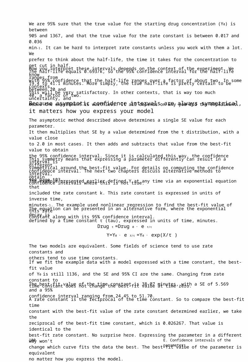
We are 95% sure that the true value for the starting drug concentration (Y0) is between905 and 1367, and that the true value for the rate constant is between 0.017 and 0.036min-1. It can be hard to interpret rate constants unless you work with them a lot. Weprefer to think about the half-life, the time it takes for the concentration to get cut in half.The half-life equals 0.693/k, so the 95% confidence interval for the half-life ranges from19.4 to 41.1 minutes. More simply, the true half-life is pretty certain to be between 20 and40, a factor of two.

How you interpret these intervals depends on the context of the experiment. We knowwith 95% confidence that the half-life ranges over a factor of about two. In some contexts,this will be very satisfactory. In other contexts, that is way too much uncertainty, andmeans the experiment is worthless. It all depends on why you did the experiment.

Because asymptotic confidence intervals are always symmetrical,it matters how you express your modelThe asymptotic method described above determines a single SE value for each parameter.It then multiplies that SE by a value determined from the t distribution, with a value closeto 2.0 in most cases. It then adds and subtracts that value from the best-fit value to obtainthe 95% confidence interval. Since it is calculated this way, the confidence interval issymmetrical around the best-fit value. For details on computing the confidence interval,see page 103.

This symmetry means that expressing a parameter differently can result in a differentconfidence interval. The next two chapters discuss alternative methods to obtainconfidence intervals where this is not true.

The example presented earlier defined Y at any time via an exponential equation thatincluded the rate constant k. This rate constant is expressed in units of inverse time,minutes-1. The example used nonlinear regression to find the best-fit value of this rateconstant along with its 95% confidence interval.

The equation can be presented in an alternative form, where the exponential decay isdefined by a time constant τ (tau), expressed in units of time, minutes.

Drug t =Drug 0 ⋅ e t/τ

Y=Y0 ⋅ e X/τ =Y0 ⋅ exp(X/τ )

The two models are equivalent. Some fields of science tend to use rate constants andothers tend to use time constants.

If we fit the example data with a model expressed with a time constant, the best-fit valueof Y0 is still 1136, and the SE and 95% CI are the same. Changing from rate constant totime constant does not change the best-fit value at time zero.

The best-fit value of the time constant is 38.07 minutes, with a SE of 5.569 and a 95%confidence interval ranging from 24.45 to 51.70.

A rate constant is the reciprocal of the time constant. So to compare the best-fit timeconstant with the best-fit value of the rate constant determined earlier, we take thereciprocal of the best-fit time constant, which is 0.026267. That value is identical to thebest-fit rate constant. No surprise here. Expressing the parameter in a different way won’tchange which curve fits the data the best. The best-fit value of the parameter is equivalentno matter how you express the model.


Taking the reciprocal of each end of the confidence interval of the time constant, we get aconfidence interval of the rate constant ranging from 0.0193 to 0.0409. As you can seemore easily on the graph below, the two confidence intervals are not the same. Ourdecision to express the model using a rate constant or a time constant affected theconfidence interval.

Fit rate constant, with 95%CI.

Fit time constant, with 95%CI.(converted to rate constant scale)

0.00 0.01 0.02 0.03 0.04 0.05Rate constant

The graph above showed the results as rate constants. The graph below shows theconfidence intervals as time constants. If you fit the time constant, the confidence interval(expressed as a time constant) is symmetrical. If you fit the rate constant, and thentransform the results to display as time constants, the 95% confidence interval is notsymmetrical.

Fit rate constant, with 95%CI.(converted to time constantscale)

Fit time constant, with 95%CI.

0 10 20 30 40 50 60 70Time constant

It is a bit disconcerting that our choice of how to express the parameter also determines,to some extent, the confidence interval. This is a fundamental problem with asymptoticconfidence intervals. But in this example, note that the difference between the twoconfidence intervals is not huge, and won’t greatly change how you interpret the results.

Christopoulos (Trends Pharmacol. Sci, 19:351-357, 1998) has used simulations to comparevarious forms of commonly used pharmacological model parameters to figure out whichform gives more valid confidence intervals. He found that certain commonly-usedparameters, such as drug affinity (e.g., Kd, Kb, Ki, etc) or drug potency (e.g., EC50), are onlyassociated with valid asymptotic confidence intervals if non-linear regression isperformed using models where these parameters are expressed as logarithms (e.g.,LogEC50). So, with respect to the reliability of the error associated with model parameters,it really does matter how you express your parameters.


Problems with asymptotic standard errors and confidenceintervalsAsymptotic confidence intervals are only approximately correct. In addition to theproblem discussed in the previous section (the intervals are always symmetrical), thereare two other issues.

• They are based on a mathematical simplification. When applied to nonlinearequations, the method is an approximation. If you have plenty of data thatclearly define the curve without a huge amount of scatter, the approximationis a good one. The confidence intervals give you a good sense of how preciselyyour data define the parameters. With marginal data, the approximationdoesn’t always work so well.

By looking at the standard error and confidence interval for each parameter,you won’t learn about the relationships between parameters. Thecalculations don’t completely take into account the degree to which theparameters are intertwined. As you’ll see in the next two chapters, best-fitparameters are often not independent.

•

Despite these problems, the asymptotic standard error and confidence intervals reportedby most nonlinear regression programs have proven to be very useful in giving you a goodsense of how precisely you know the parameters.

The next two chapters explain alternative methods to compute confidence intervals, andChapter 19 compares the methods.

What if your program reports “standard deviations” instead of“standard errors”?Some programs report a standard deviation for each parameter rather than a standarderror. In this context (uncertainty of best-fit values determined by regression), there is nodistinction between the standard error and standard deviation.

The term standard error can be used to quantify how precisely you know a computedvalue. For example, the standard error of the mean tells you how uncertain that mean is.Its value depends on the number of data points and their scatter (as quantified by thestandard deviation). The standard error of a mean is your best estimate for the value youwould obtain if you repeated the experiment many times, obtaining a different mean foreach experiment, and then computed the standard deviation of those means. So thestandard error of a mean can also be called the standard deviation of the mean (but it isvery different from the standard deviation of the data).

Similarly, the standard error of a slope is an assessment of how precisely you havedetermined that slope. It is your best estimate for the value you would obtain if yourepeated the experiment many times, obtained a different slope for each experiment, andthen computed the standard deviation of those slopes. You could also call that value thestandard deviation of the slope.

It is more conventional to refer to the standard error of a parameter rather than thestandard deviation of a parameter.


How to compute confidence intervals from standard errorsIf your program doesn’t report the 95% confidence intervals of the parameters, it is easyto compute them by hand. The confidence interval of each parameter is computed fromthe best-fit value and the SE of those best-fit values using this equation:

BestFit - t * ⋅ SE to BestFit + t * ⋅ SE

If you didn’t constrain the parameter, the confidence interval is always centered at thebest fit value and extends the same distance above and below it. This distance equals thestandard error of the parameter (discussed in the previous section) times the constant t*.This value comes from the t distribution, and depends on the amount of confidence youwant (usually 95%, but you could choose some other value) and the number of degrees offreedom (df). For nonlinear regression, df equals the number of data points minus thenumber of parameters fit by nonlinear regression.

You can find the value of t* in tables in most statistics books. If you have plenty of degreesof freedom (more than a dozen or so), t* will have a value near 2.0. You can find the valueof t* for 95% confidence intervals using this Excel formula (substitute 0.01 for 0.05 to getthe value of t* to compute 99% confidence intervals).

=TINV(0.05,df)

Our example had 8 data points and 2 parameters, and so has 6 degrees of freedom. Thevalue of t* (for 95% confidence) is 2.4469. If you had more data (more degrees offreedom) this value would be lower. As degrees of freedom increase, t* (for 95%confidence) approaches 1.96.


17. Generating confidence intervals by MonteCarlo simulations

An overview of confidence intervals via Monte Carlo simulationsAs discussed in the previous chapter, the asymptotic method built in to most nonlinearregression programs is only an approximate method to determine the confidence intervalof a best-fit parameter. This chapter presents one alternative method, and the nextchapter presents still another alternative method.

The idea here is to simulate a bunch of data sets, each with different random scatter. Thenfit each simulated data set to determine the best-fit values of the parameters. Finally, we’lluse the distribution of best-fit parameters among the simulated data sets to createconfidence intervals.

This approach for determining confidence intervals is called Monte Carlo simulations.

Monte Carlo confidence intervals

General ideaFrom the curve fitting results in the previous chapter, we know the best-fit values of Y0and k. The curve fitting program also reports Sy.x, which is the best-fit estimate of thestandard deviation of the residuals. Its value is computed from the sum-of-squares, thenumber of data points and number of parameters (see page 33). It quantifies how muchthe data are scattered around the curve.

Follow these steps to determine the confidence intervals by Monte Carlo simulation:

1. Generate an ideal data set. Use the same X values as used in the actual data.Generate the Y values using the same model you used to fit the experimental data(an exponential decay model in this case). Use the best-fit values from nonlinearregression of the experimental data, as the ideal parameters (k=0.02626 andY0=1136 for this example) to generate the ideal data.

Add random scatter. To each ideal point, add random scatter drawn from aGaussian distribution with a mean of zero and an SD equal to the value of Sy.xreported by nonlinear regression of our experimental data. For this example, wewant to choose random numbers with a standard deviation of 105.3 (the reportedSy.x from the fit of our experimental data).

Fit the simulated data with nonlinear regression, and record the best-fit value ofeach parameter. Here are the first two such simulated data sets, along with thebest-fit curves.

2.

3.


1500

SPANK

10690.02413

1500

SPANK

13580.02659

[Drug]

500

[Drug]

0 25 50 75 100

1000 1000

500

0 0

0 25 50 75 100Minutes Minutes

4. Repeat steps 2 and 3 many (perhaps 1000) times. Each time, compute new randomnumbers so each of the simulated experiments has different data. The idea here isthat these simulated data sets are similar to what you would have observed if yourepeated the experiment many times.

Find the 2.5 and 97.5 percentile values for each parameter. The range betweenthese values is the confidence interval.

5.

Confidence interval of the rate constantHere is a graph of the frequency distribution for the 1000 rate constants determined from1000 randomly generated data sets.

125

Number of simulated experiments

100

75

50

25

0 010. 5010. 6010. 7010. 8010. 9020. 0020. 1020. 2020. 3020. 4020. 5020. 6020. 7020. 8020. 9030. 0030. 1030. 2030. 3030. 4030. 5030. 6030. 7030. 8030. 9040. 0040. 10420.

Best-fit value of rate constant

We chose to simulate 1000 experiments. If we had simulated more experiments, thefrequency distribution might have been smoother. To obtain the 95% confidence interval,we sort the 1000 best-fit values, and remove the 25 (2.5%) at each end. The range of therest is the 95% confidence interval for the rate constant, which extends from .01970 to.03448.

We repeated the simulations with 10,000 (rather than 1000) simulated data sets, and the95% confidence interval was about the same. It went from 0.01948 to 0.03520.

Note that this method of obtaining the confidence interval creates intervals that are notnecessarily symmetrical around the best-fit value. These intervals also don’t depend on

17. Generating confidence intervals by Monte Carlo simulations 105

how we express the model. We could have fit each of the simulated data sets to a modelexpressed in terms of time constant instead of rate constant. Each simulated data setwould have a best-fit value of the time constant that is the reciprocal of the best-fit valueof the rate constant. Rank the one thousand best-fit values of the time constant, removethe 25 highest and lowest values, and you’ll get the confidence interval of the timeconstant. This is completely equivalent to taking the inverse of each end of the confidenceinterval of the rate constant.

Our decision to express the model in terms of rate constant or time constant affected onlyhow the confidence intervals are presented. With Monte Carlo simulations (unlike theasymptotic method built-in to most nonlinear regression programs), you’ll get equivalentintervals no matter how you choose to express the parameter.

Confidence interval of Y0

Here is a graph of the frequency distribution for the 1000 values of Y0 determined from1000 randomly generated data sets.

125

Number of simulated experiments100

75

50

25

0 8008258508759009259509710 5010 0210 5510 0711 5011 0211 5511 0712 5012 0212 5512 0713 5013 0213 5513 0714 5014 0214 5514 075

Best-fit value of Y0

To obtain the 95% confidence interval, we sort the 1000 best-fit values, and remove the 25at each end. The range of the rest is the 95% confidence interval, which extends from 964to 1317.

When we repeated the simulations with 10,000 (rather than 1000) simulated data sets,the 95% confidence interval extends from 956 to 1328 (about the same).

Monte Carlo simulations shows how the two parameters are relatedSo far, we have determined a confidence interval for each parameter separately. But thetwo parameters are related. Here is a graph of our one thousand simulated experiments,showing the best-fit value of rate constant and Y0. Each dot is the result of analyzing onesimulated data set, plotting the best-fit value of the rate constant on the X axis and thebest-fit value of Y0 on the Y axis.


1450

1350

1250

1150

1050

950

850

750

0.01 0.02 0.03 0.04 0.05

Y0

Rate constant

The relation between parameters makes sense. If the true Y0 is larger, that means there ismore drug in the plasma at time zero. Therefore, the rate constant is likely to be larger(faster drug elimination). If the true Y0 is smaller (less drug), there is less drug present sothe rate constant is likely to be lower (slower elimination).

Perspective on Monte Carlo methodsIf you are encountering Monte Carlo methods for the first time, you may think that it isessentially magic. You start with one data set, simulate lots of “data sets” that aren’t reallydata, and then use the analyses of those simulated data sets to learn about the uncertaintyin the parameters you estimated from the actual data.

This method has a solid mathematical foundation (plenty of theorems have been proven)and has been shown to be useful in practice. Although this method seems strange whenyou first hear about it, it really does work.

How to perform Monte Carlo simulations with PrismIt isn’t hard to do the Monte Carlo simulations with Prism. Use the “Simulate data”analysis to generate a simulated data set. You’ll need to choose the X values, the model,the parameters, and the SD of random scatter. For parameters, enter the best-fit valuesfrom fitting your data. For SD of the random scatter, enter the Sy.x reported by nonlinearregression. Choose Gaussian error.

This “analysis” will create a results table with the simulated data. From that table, clickAnalyze, choose nonlinear regression, and pick the model and choices just as if youanalyzed the original data.

To simulate 1000 data sets, you need to run a script (a choice on the File menu). Here isthe Prism script we used for the first example:

17. Generating confidence intervals by Monte Carlo simulations 107

shortlogsetpath "c:\temp"Openoutput "Monte Carlo CI.txt" Clearwtext "Top" ;wtext "K"Foreach 1000 GoTo R 1 regenerate GoTo R 2 Wcell 3,1; wcell 4,1Next

The first line says not to create a detailed log. The next two lines define the folder and filethat will contain the results. The next two lines write a header on top of the file. Then theloop starts, to create 1000 data sets. Of course, you can increase that number to get moreprecise confidence intervals. For each loop, the script goes to the first results page (thesimulation) and regenerates it (new random numbers). Then it goes to the second resultspage (the nonlinear regression results) and records the values in the first column, thirdand fourth row (values of K and Y0 for our example; you may need to adjust the rownumbers).

Tip: Read about Prism scripts in the last chapter of the Prism 4 User’s Guide.

After the script is finished (a few minutes), import the resulting 1000 row text file intoExcel. To determine the 2.5 and 95.7 percentiles from a list of values in column B, usethese Excel equations.

=Percentile(B:B, 0.025)=Percentile(B:B, 0.975)

Variations of the Monte Carlo methodThe method presented in this chapter is not the only way to do Monte Carlo simulations togenerate confidence intervals of best-fit parameters. Here are some choices you havewhen programming a Monte Carlo simulation:

• Add random error to what? With each simulation, you can add random errorto the actual experimental data, or you can add random data to ideal datapredicted from the model.

How do you generate the random error? In our discussion, we generated therandom error from a Gaussian distribution. This makes a lot of sense, butrequires assuming that the scatter of data around the curve does indeedfollow a Gaussian distribution. One alternative is to bootstrap the errors.Create a list of residuals – the vertical distances of the data from the best-fitcurve. Now for each simulation, for each data point, randomly choose one ofthose residuals. You don’t generate new random error. Instead, yourandomly reapply the actual residuals observed in the experiment.

How do you generate the confidence interval? We used the 2.5 and 97.5percentiles. Other methods are possible.

•

•


18. Generating confidence intervals via modelcomparison

Overview on using model comparison to generate confidenceintervalsIn this chapter, we’ll develop a third method to obtain the confidence interval of a best-fitparameter (to complement the asymptotic and Monte Carlo methods described in theprevious two chapters). It is based on the method to be discussed below in Chapter 22.That chapter explains how to compare two related fits to a set of data. This methodgenerates an F ratio, from which you can determine a P value. If the P value is less than0.05, we say that the fit of the two models differs significantly.

Conceptually, it isn’t hard to use that method to develop confidence intervals for the best-fit parameters. If we change the value of the parameters from their best-fit values, weknow the fit will get worse. But how much worse? We’ll compare this new fit with the best-fit curve determined by nonlinear regression. If the P value is greater than 0.05, than thisnew fit is not significantly worse, so this set of parameter values must be within ourconfidence interval. If the P value is less than 0.05, then the new parameter values lead toa curve that fits the data significantly worse than the best-fit values, so these parametersare outside the confidence interval.

A simple example with one parameterLater in this chapter we’ll return to the example used in the previous two chapters. Butfirst, let’s go back to a simpler example (see page 91) where there is only one parameter tofit.

We measured a signal over time and normalized the results to run from 100% at time zeroto 0 at infinite times. We fit this to an exponential decay model, fixing the top to 100 andthe bottom plateau to 0, leaving only one parameter, the rate constant, to fit. The best-fitvalue of k is 0.3874 min-1. How precisely do we know this value of k? Let’s see how thesum-of-squares varies as we change the value of k.

18. Generating confidence intervals via model comparison 109

3000

Sum-of-squares2000

1000

0

0.2 0.3 0.4 0.5 0.6 0.7Possible value of k (min-1)

The graph above plots sum-of-squares (a measure of how well the curve fits the data) aswe vary the value of the rate constant k. The best-fit value of k, 0.3874 min-1) is the valuewhere the sum-of-squares is lowest.

The model comparison method for generating a confidence interval is based on the graphabove. Chapter 22 shows how to compare two curves and calculate F using this equation.

F= (SSnull -SSalt )/SSalt

(DFnull -DFalt )/DFalt

In this context, substitute SSbest-fit for SSalt, This is the sum-of-squares of the curvedetermined by nonlinear regression. Also substitute SSall-fixed for SSnull. This is the sum-of-squares when we fix all the parameters (in this example, there is only one parameter) to afixed value we choose. Also substitute N-P for DFalt and N for DFnull, where N is thenumber of data points and P is the number of parameters (don’t mix this up with the Pvalue). Now the equation looks like this:

F= (SSall-fixed -SSbest-fit )/SSbest-fit

P/(N-P)

SSall-fixed −1 SSbest-fit = P/(N-P)

This equation is usually used to compare two fits -- to compute F from which we obtain aP value. Here, we are want to work backwards to get a confidence interval. We are strivingfor a 95% confidence interval, so we want the P value to equal 0.05. To get this P value, weknow (can look up) the value of F we need. So F is a constant we set, not a variable wecompute. Similarly SSbest-fit is always the same, as determined by our data and model. Wegot its value by using nonlinear regression. We also know the values of N (number of datapoints) and P (number of parameters). What we need to do is find values of the rateconstant that create a curve where the sum-of-squares equals SSall-fixed. So let’s rewrite theequation, putting SSall-fixed on the left.

PSSall-fixed =SSbest-fit F+1 N-P

Now we know the values of all the variables on the right.


Variable Comment ValueSSbest-fit

P

Sum-of-squares when nonlinear regression fits thecurve, adjusting both parameters.

Number of parameters. We are fitting the rateconstant (k) and the value of Y at time zero (Y0) soP=2. Don’t confuse this use of the variable P with aP value.

Number of data points. We had twelve X valuesand only collected one Y value at each X, so N=12.

The critical value of the F distribution for a P valueof 0.05 (for 95% confidence) with P df in thenumerator (1 in our example) and N-P (12-1=11 inour example) degrees of freedom in thedenominator. You can look this up in a statisticstable, use the free calculator atwww.graphpad.com, or use this Excel formula:=FINV(0.05,1,11)

Computed from the other parameters in theequation. This is our target value for SS. We willvary the rate constant to achieve a sum-of-squaresequal to this target.

SS=228.97

P=1

N

F

N=12

F= 4.8483

SSall-fixed SS=329.89

What this means is that if we change the value of k a small amount, so that the resultingcurve has a sum-of-squares less than 329.89, the fit will not be significantly different thanthe fit determined by nonlinear regression. These values of k define the 95% confidenceinterval. If k is outside this range, then the resulting curve will have a sum-of-squaresgreater than 329.89 and so fit the data significantly worse.

So what range of values for k satisfies this criterion? As you can see from the graph below,a range of values of k from about 0.35 to 0.43 give sum-of-square values less than 329.9so therefore generate curves that are not significantly different (at the 5% significancelevel) than the best fit curve.

1000

Sum-of-squares

500

329.9

0

0.30 0.35 0.40 0.45 0.50Possible value of k


To compute the confidence intervals more exactly, we can alter k over a finer range ofvalues. Or, as explained below on page 116, we can use Excel’s solver to find the two valuesof k that lead to a sum-of-squares of 329.89. The confidence interval determined this wayranges from 0.3525 to 0.4266. Any value of k outside that range would result in a curvewhose fit is significantly worse than the best-fit curve. Note that this confidence interval isnot symmetrical around the best-fit value.

Confidence interval for the sample data with two parametersThe rest of this chapter shows how to apply this method to the example data used in theprevious two chapters. Since the two parameters are related, you’ll get the mostinformation by finding a confidence region – a set of values for the two parameters. We’llgo through the calculations in the next two sections. But first, the answer. The graphbelow plots various possible values of the rate constant on the X axis vs. possible values ofY0 on the Y axis. The two parameters are correlated. If the value of k is high, then thevalue of Y0 is also very likely to be high. If the value of k is low, then the value of Y0 is alsovery likely to be low.

The plus in the middle denotes the best-fit value of k and Y0 determined by nonlinearregression. The egg-shaped contour shows values of k and Y0 that generate curves that arejust barely significantly different than the best-fit curve. So any values of k and Y0 that liewithin the contour (the gray area) lead to curves that are not significantly different (at the5% significance level) than the best-fit curve. Therefore, this contour defines theconfidence interval.

The next section explains how this graph was constructed.

Using model comparison to generate a confidence contour for theexample dataThe method to be discussed below in Chapter 22 lets you compare two fits (to one set ofdata) by looking at the difference between sum-of-squares. This method computes an Fratio, which leads to a P value.


We will repeatedly compare the sum-of-squares from curves defined by two sets ofparameters.

One curve is always defined by the best-fit results obtained by nonlinear regression. Callthe number of parameters you fit to be P. Call the sum-of-squares from this fit to beSSbest-fit.

The other curve will change as we repeatedly apply the method. To create this curve, wewill fix all of the parameters to constant values. You’ll see soon how we pick these values.Since we set all the parameter to fixed (constant) values, we don’t ask the program to fitanything. Instead, we only ask a program to compute the sum-of-squares. Call this sum-of-squares SSall-fixed.

Compare the fits using an equation explained earlier in this chapter.


For this example, here are the values.


P

Sum-of-squares when nonlinear regression fits thecurve, adjusting both parameters.

Number of parameters. We are fitting the rateconstant (k) and the value of Y at time zero (Y0) soP=2. Don’t confuse this use of the variable P with aP value.

Number of data points. We had eight X values andonly collected one Y value at each X, so N=8.

The critical value of the F distribution for a P valueof 0.05 (for 95% confidence) with P df in thenumerator (2 in our example) and N-P (8-2=6 inour example) degrees of freedom in thedenominator. You can look this up in a statisticstable, use the free calculator atwww.graphpad.com, or use this Excel formula:=FINV(0.05,2,6)

Computed from the other parameters in theequation. This is our target value for SS. We willvary parameters to achieve a sum-of-squares equalto this target.

SS= 66489.16

P=2

N

F

N=8

F= 5.1432


We want to vary one parameter, holding the rest constant, increasing SS until it gets to180479.3. When it reaches that value, we know that F will equal 5.1432, so the P value willequal 0.05. This target value for SSall-fixed was computed from the equation above.

Let’s start by holding Y0 constant at its best-fit value of 1136, and gradually decrease k. Asyou reduce the value of k from the best-fit value, the curve will get further from the datapoints, so the sum-of-squares will go up. Adjust the value of k until the sum-of-squares


equals 180479.3. This happens when k= 0.01820. We plot on the graph below the pointk=0.01820, Y0=1136.

Now let’s increase the value of k from its best-fit value until the sum-of-squares again hitsthat target value. This happens when k= 0.04002. Add to the point k=0.04002, Y0=1136to the graph we are building (below).

You might think we have determined the confidence interval of k as ranging from 0.01820to 0.04002. But this isn’t really the confidence interval we care about. It is the confidenceinterval of k, assuming that Y0 equals exactly 1136 (its best-fit value). But Y0 is itselfsubject to variation. What you want to know is the lowest and highest values of k thatgenerate the target value of SS at any value of Y0.

Now let’s fix the rate constant at its best-fit value, and increase and decrease Y0 until thesum-of-squares is 180479.3. That happens when Y0 equals 886.5 and 1385.5. We’ll addtwo more points to the graph, at k=0.02626, Y0=886.5 and k=0.02626, Y0=1385.5. Thegraph below now shows four pairs of values of k and Y0 where the sum-of-squares is180479.3., along with lines showing the best-fit values of Y0 and k.

1500

1250

Y0

1000

750

0.01 0.02 0.03 0.04 0.05

Rate constant, k

Let’s continue this process. We hold one parameter constant (to various values) and findthe two values of the other parameter that make the sum-of-squares equal 180479.3. Thenhold the first parameter constant to a different value, and again find two values of theother parameter that makes the sum-of-squares meet the target value. It doesn’t reallymatter if you hold k constant and vary Y0 or hold Y0 constant and vary k. The graph belowwas made using a combination of the two methods. Repeat with many sets of values, andhere is the result. (The next section explains how we used Excel to facilitate thesecalculations.)

1500

1250

Y0

1000

750

0.01 0.02 0.03 0.04 0.05

Rate constant, k


The plus in the middle of the graph represents the best-fit values of k and Y0. Each pointrepresents a pair of values for k and Y0 that define a curve that is far enough from oursample data so the sum-of-squares equals 180479.3. If you compare the fit of any curvedefined by the parameter values graphed here with the best-fit nonlinear regression curve,the F ratio equals 5.143 so the P value equals 0.05. Even though the shape (in thisexample) looks more like an egg than an ellipse, it is often called a confidence ellipse. Abetter term is confidence contour.

Any pair of values of k and Y0 that is outside the contour define a curve that is fartherfrom the points, and generates a higher sum-of-squares. Therefore the value of F is largerthan 5.143 and so the P value is less than 0.05. These values of k and Y0 define curves thatfit the data significantly worse than the best-fit curve. Any pair of k and Y0 that is insidethe contour defines a curve that is further from the points than the best-fit curve. But if wecompare the two curves, the F ratio will be less than 5.143 so the P value is greater than0.05. The curves generated by parameter values inside the egg do not fit the datasignificantly worse than the best-fit values. Therefore we are 95% sure that the true valueof k and Y0 lies inside the confidence contour.

Converting the confidence contour into confidence intervals forthe parametersTo find the 95% CI for k, we find the lowest and highest values of k on the contour, asshown in the figure below. The 95% CI of the rate constant determined this way rangesfrom 0.0159 to 0.0420.

95%CI of k

1500

1250

Y0

1000

750

0.01 0.02 0.03 0.04 0.05

Rate constant, k

To find the 95% confidence interval for Y0, we find the lowest and highest values of Y0 onthe contour, as shown below. The 95% confidence interval for Y0 ranges from 844.00 to1442.75.


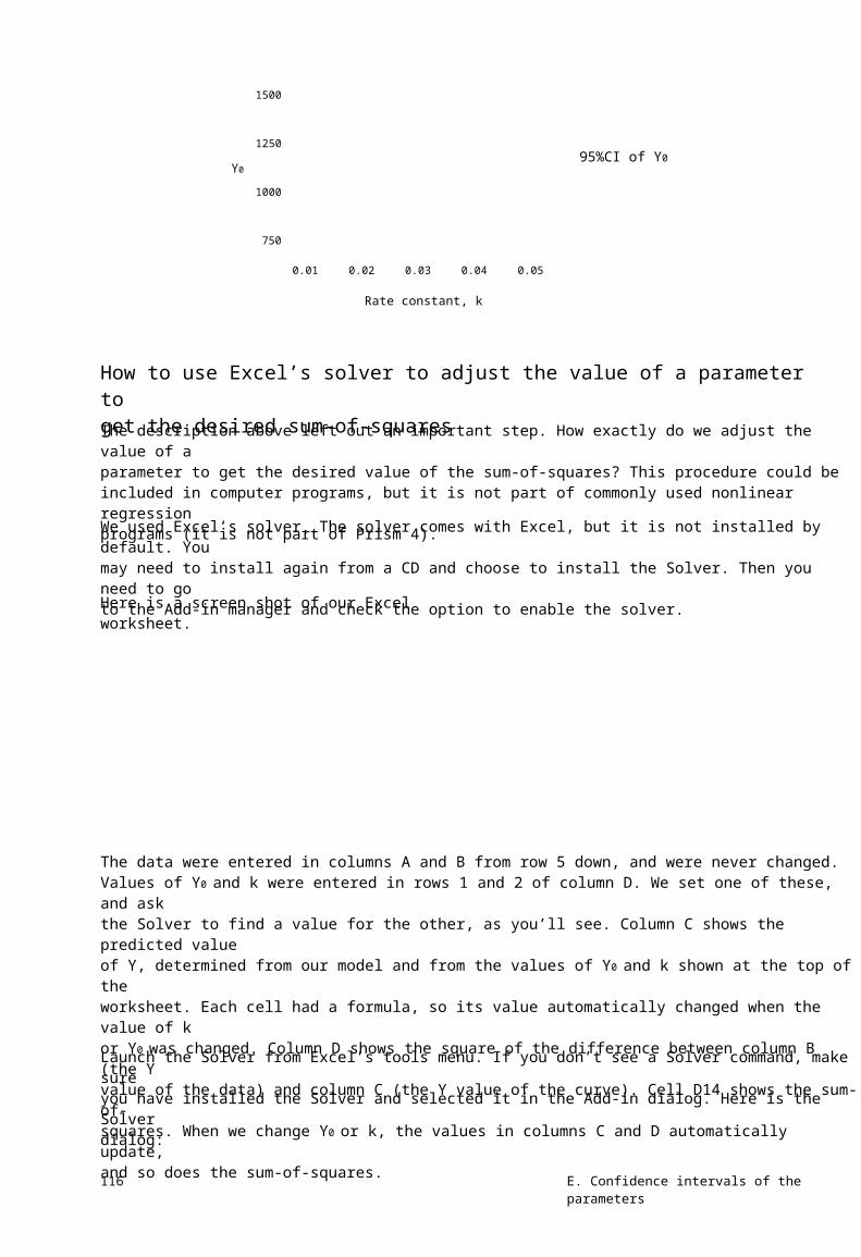
1500

1250

Y095%CI of Y0

1000

750

0.01 0.02 0.03 0.04 0.05

Rate constant, k

How to use Excel’s solver to adjust the value of a parameter toget the desired sum-of-squaresThe description above left out an important step. How exactly do we adjust the value of aparameter to get the desired value of the sum-of-squares? This procedure could beincluded in computer programs, but it is not part of commonly used nonlinear regressionprograms (it is not part of Prism 4).

We used Excel’s solver. The solver comes with Excel, but it is not installed by default. Youmay need to install again from a CD and choose to install the Solver. Then you need to goto the Add-in manager and check the option to enable the solver.

Here is a screen shot of our Excel worksheet.

The data were entered in columns A and B from row 5 down, and were never changed.Values of Y0 and k were entered in rows 1 and 2 of column D. We set one of these, and askthe Solver to find a value for the other, as you’ll see. Column C shows the predicted valueof Y, determined from our model and from the values of Y0 and k shown at the top of theworksheet. Each cell had a formula, so its value automatically changed when the value of kor Y0 was changed. Column D shows the square of the difference between column B (the Yvalue of the data) and column C (the Y value of the curve). Cell D14 shows the sum-of-squares. When we change Y0 or k, the values in columns C and D automatically update,and so does the sum-of-squares.

Launch the Solver from Excel’s tools menu. If you don’t see a Solver command, make sureyou have installed the Solver and selected it in the Add-in dialog. Here is the Solverdialog:


Here we ask it to adjust the value of cell $D$1 (the value of Y0) in order to get the value ofcell $D$14 (the sum-of-squares) to equal 180479.3 (the target we computed above). Therewill be two values of Y0 that work, so we give the Solver the constraint that Y0 (cell D1)must be greater than 1200. Click Solve. Excel tells you that the Solver found a solution.

Click OK, and Prism changes the value of Y0 to 1216.7, which leads to a sum-of-squares (asrequested) of 180479.3.

Now we have determined one set of values for Y0 and k (1216.7 and 0.0200) that definesone point on our graph.

Repeat this process for many values of k, and then repeat again with the same values of kbut with the opposite constraint (Y0<1200) and you’ll create enough points to define theegg shown earlier.

Instead of constraining the value of Y0, you can simply change the starting value (thevalue you enter into cell D1). There are two solutions to the problem, and the Solver willalmost always find the solution that is closest to the starting value. So run the Solvertwice, once starting with a high value of Y0 and once starting with a low value of Y0.

More than two parametersIf you are fitting more than two parameters, it becomes much harder to apply thismethod. And it even becomes hard to figure out how to display the results. But the idea isstill the same. You want to find all sets of parameters that define curves whose sum-of-squares is just enough worse than the sum-of-squares of the best-fit curve so that an F testgives a P value of 0.05.

19. Comparing the three methods for creatingconfidence intervals

Comparing the three methods for our first exampleThe last three chapters presented three distinct methods for obtaining confidenceintervals from our sample data.

The three methods gave similar, but not identical, results as shown in this graph.

Asymptotic method

Monte-Carlo simulations

Model comparison

0.00 0.01 0.02 0.03 0.04 0.05Rate constant

The simple method always gives a confidence interval that is symmetrical and tends to bea bit optimistic (too narrow). Monte Carlo simulations also tend to be a bit optimistic –the interval is too narrow. The model comparison method (via F test) is probably the mostaccurate method, but is also most cumbersome.

Here is the comparison, showing the time constant rather than the rate constant.

Asymptotic method


Model comparison

0 10 20 30 40 50 60 70Time constant

Here is the comparison of the three different methods to compute the confidence intervalsof Y0.


Asymptotic method


Model comparison

0 500 1000 1500Value of Y0

Here we superimpose the egg shape determined by model comparison (circles) with theresults determined by Monte Carlo simulations (plusses). The two have a very similarshape, but the Monte Carlo simulations are a bit more compact.

1450

1350

1250

1150

1050

950

850

750

0.01 0.02 0.03 0.04 0.05

Y0

Rate constant

A second example. Enzyme kinetics.This example shows enzyme activity as a function of substrate concentration. There areonly seven data points, and the experiment does not use high enough substrateconcentrations to properly define the maximum velocity.

30

Enzyme Velocity

[Substrate] 0.5 1.0 2.0 3.0 4.0 6.0 8.0

Velocity 2.7 11.3 10.3 19.0 16.0 25.0 27.0

20

10

0 0.0 2.5 5.0 7.5 10.0

[Substrate]

We fit the data to this model:

19. Comparing the three methods for creating confidence intervals 119

Velocity=Velocity max ⋅ [Substrate] K M +[Substrate]

Y=Vmax ⋅ XK M +X

Asymptotic (approximate) standard errors and confidence intervalsThe best-fit parameter values, with their standard errors and confidence intervals areshown in the table below. The sum-of-squares is 42.3, and Sy.x is 2.909.

Parameter Best-fit value Standard Error 95% CIVmax

Km

42.40

4.687

10.81

2.374

14.61 to 70.19

-1.42 to 10.79

The confidence interval for Vmax is pretty wide, telling you what you already knew -- thatthis experiment wasn’t designed very well so doesn’t define Vmax very well. The asymptoticconfidence interval is symmetrical around the best-fit value, as it must be (given how it iscomputed). But the lower limit doesn’t make much sense. It is too low -- lower than half ofthe Y values in the data.

The Km is the concentration of substrate that leads to half-maximal enzyme velocity. Theconfidence interval for Km extends down to negative values. Since this is nonsense, we’lltruncate it to 0.0 to 10.79. This means that the Km could be anywhere in the range ofconcentrations we used, which means this experiment gave us no real information on thevalue of Km.

Monte Carlo confidence intervalsUsing the Monte Carlo method, the 95% confidence interval for Vmax ranged from 25.78 to92.88. The 95% confidence interval for Km ranged from 1.376 to 16.13.

The two parameters are extremely related, as this graph shows. Each point represents thebest-fit value of Vmax (X axis) and Km (Y axis) for one simulated data set. The left panelshows the results of all thousand simulations. The right panel drops the results of a fewdozen simulations to emphasize the bulk of the results.


959085807570656055504540353025201510 5 0

0 100 200 300 400 500

20

15

KMKM 10

5

00 25 50 75 100

Vmax Vmax

Confidence intervals via model comparisonAgain, we’ll compare the best-fit curve generated by nonlinear regression with the fit of acurve where both parameters are fixed to values we select. Again, we’ll use the equationbelow to figure out the sum-of-squares needed to make a fit be different enough that its Fvalue is high enough to yield a P value of exactly 0.05.



P

N

F

Sum-of-squares from nonlinearregression.

Number of parameters.

Number of data points.

The critical value of the F distributionfor a P value of 0.05 (for 95%confidence) with P df in thenumerator (2 in our example) and N-P(7-2=5 in our example) degrees offreedom in the denominator.

Computed from the other parametersin the equation. This is our targetvalue for SS.

SS= 42.303

P=2

N=7

F= 5.7861


We set Km to various values, and used Excel’s Solver (see page 116) to find two values ofVmax (for each Km) that lead to the target sum-of-squares. The graph below shows the bestfit values of Vmax and Km as the horizontal and vertical line. Each point on the graphrepresents a pair of values for Vmax and Km that cause the sum-of-squares to equal thetarget value and so define the 95% confidence interval.


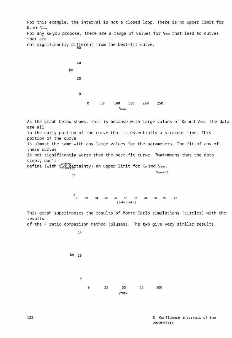
For this example, the interval is not a closed loop. There is no upper limit for Km or Vmax.For any Km you propose, there are a range of values for Vmax that lead to curves that arenot significantly different from the best-fit curve.

60

40KM

20

0

0 50 100 150 200 250Vmax

As the graph below shows, this is because with large values of Km and Vmax, the data are allin the early portion of the curve that is essentially a straight line. This portion of the curveis almost the same with any large values for the parameters. The fit of any of these curvesis not significantly worse than the best-fit curve. That means that the data simply don’tdefine (with 95% certainty) an upper limit for Km and Vmax.

100 Vmax=100

Enzyme Velocity

50Vmax=50

00 10 20 30 40 50 60 70 80 90 100

[Substrate]

This graph superimposes the results of Monte Carlo simulations (circles) with the resultsof the F ratio comparison method (pluses). The two give very similar results.

20

KM 10

0

0 25 50 75 100Vmax


Comparing the confidence interval of the three methodsThis graph compares the three methods used to determine the 95% confidence interval forVmax. Note that the third method (compare fits with F ratio) has no upper limit.

Asymptotic method


Model comparisons

0 25 50 75 100Value of Vmax

This graph compares the three methods used to determine the 95% confidence interval ofthe Km. Again, note that the third method (model comparison with F ratio) has no upperlimit.

Asymptotic method


Model comparisons

0 5 10 15 20Value of Km

In this example, our data simply don’t define the curve. The most accurate method,comparison with F ratio, simply can’t find an upper limit for either parameter.

For this example, the standard method built-in to nonlinear regression programs givesyou a confidence interval that is somewhat misleading. But an alert scientist would noticetwo things:

• The lower confidence limit for Vmax is obviously too low, since it is lower thanhalf the data points. Since the confidence intervals must by symmetrical, ifone limit is too low, the other limit must not be high enough.

The confidence interval for Km includes all the substrate concentrations usedin the experiment (the confidence interval goes up to 12, but the highestconcentration used in the experiment is 8).

•

Even though we can’t interpret the asymptotic confidence intervals literally, they tell uswhat we need to know – that our data don’t define Km or Vmax very well.

A third exampleHere is a third example. This is a dose response curve without too much scatter.


log(conc)

-9.0-8.5-8.0-7.5-7.0-6.5-6.0-5.5-5.0-4.5-4.0-3.5-3.0

Percent ResponeY1Y2Y3 8.711.4-2.0 9.42.71.5 3.14.9-1.9 24.423.79.0 30.236.139.1 60.665.048.4 72.867.776.3 77.676.276.9100.788.591.0 97.298.094.6102.4107.2106.6114.1108.8100.5 98.693.3104.3

100%

75%

50%

25%

0%

Response

-9 -8 -7 -6 -5 -4 -3

log(conc)

The results were normalized to run from 0 to 100. We fit a sigmoidal dose-response curveto find the best-fit values of the logEC50 (the concentration that gives a 50% response; themiddle of the curve) and the Hill Slope (a measure of how steep the curve is). We fixed thebottom plateau to 0.0 and the top to 100.0, so only fit two parameters (the logEC50 andthe Hill Slope). The triplicate values were treated as separate data points, so there a totalof 39 points, so 37 degrees of freedom (39 data points minus two parameters to fit).

Note: We normalized the data to control values so the data run from 0 to 100.But there is random variation, so some data points have normalized values lessthan zero and others have normalized values that greater than one hundred. Weleft those in to avoid biasing the analyses.

Asymptotic standard errors and confidence intervalsHere are the standard errors and confidence intervals, as computed by the standardmethod built-in to all nonlinear regression programs. The sum-of-squares is 1644.2 andthe Sy.x is 6.6661.

Parameter Best-fit value Standard Error 95% CILogEC50

Hill Slope

-6.590

0.6996

0.05264

0.05237

-6.697 to -6.484

0.5934 to 0.8057

Monte Carlo simulationsThe results of Monte Carlo simulations are graphed below. The two parameters are notrelated. The 95% confidence interval for the logEC50 ranges from -6.687 to -6.484. The95% confidence interval for the Hill Slope ranges from 0.6077 to 0.8231. These confidenceintervals are very close to those determined by the simple method built in to nonlinearregression programs.


1.0

0.9

Hill Slope0.8

0.7

0.6

0.5

-6.75 -6.65 -6.55 -6.45 -6.35logEC50

Method comparison via F testHere are the values we used to find confidence interval via model comparison.



P

N

F

Sum-of-squares from nonlinear regression.

Number of parameters.

Number of data points.

The critical value of the F distribution for a Pvalue of 0.05 (for 95% confidence) with P df inthe numerator (2 in our example) and N-P(39-2=37) df in the denominator.

Computed from the other parameters in theequation. This is our target value for SS.

SS= 1644.2

P=2

N=39

F= 3.252


Here are the results. Each point represents a pair of values for logEC50 and Slope thatgenerate a curve whose sum-of-squares is just enough different from the best-fit curve togive a F ratio of 3.252 and thus a P value of 0.05. Any points inside the ellipse define acurve that is not significantly different from the best-fit curve. Any points outside theellipse define a curve that is significantly different from the best fit curve. The ellipse,therefore, defines our 95% confidence interval.


1.00

Hill Slope0.75

0.50 -6.75 -6.65 -6.55 -6.45 -6.35

logEC50

The 95% confidence intervals are taken from the highest and lowest value of eachparameter on the ellipse. The 95% confidence interval for the logEC50 ranges from -6.72to -6.45. The 95% confidence interval for the Hill Slope ranges from 0.59 to 0.85. Theseconfidence intervals are very close to those determined by the simple method built in tononlinear regression programs.

Comparing the three methodsThe graph below compares the confidence intervals for each parameter as generated bythe three methods. The three methods are essentially the same for all practical purposes.

Asymptotic Method

Monte Carlo

Compare fits

-6.75 -6.65 -6.55 -6.45 -6.35 0.5 0.6 0.7 0.8 0.9logEC50 Hill Slope

The graph below compares the Monte Carlo method with the method that compares fitswith the F ratio. The circles show the border of the 95% confidence region as defined bythe model comparison method. The pluses show the individual results of Monte Carlosimulations. If the methods were equivalent, you’d expect 95% of the simulated fits to liewithin the ellipse defined by the model comparison method, and that is about what yousee.


1.00

Hill Slope0.75

0.50 -6.75 -6.65 -6.55 -6.45 -6.35

logEC50

ConclusionsWhen you evaluate the results of nonlinear regression, you don’t only care about the best-fit values of the parameters. You also want to know how precisely you have determinedthem. The easiest way to do so is to look at the asymptotic confidence intervals reportedby your nonlinear regression program.

Ideally you have collected plenty of data points without too much scatter and have spacedthese sensibly over appropriate range of X. If so, the asymptotic confidence intervals willbe quite useful. As we saw in the third example above, all three methods for computingconfidence intervals give almost identical results in cases like this.

In a less ideal situation (you have collected few data points, they have a lot ofexperimental scatter, and you have chosen the X values poorly), the reported confidenceinterval will be much wider. In these cases, the asymptotic interval reported by nonlinearregression may be too narrow, too optimistic. The uncertainty may even be worse thanwhat the program reports. But the wide confidence intervals tell you what you need toknow – that you haven’t determined the parameters very well and should either collectmore data or run nonlinear regression constraining a parameter to a constant value.

It would be a mistake to assume that the “95% confidence intervals” reported by nonlinearregression have exactly a 95% chance of enclosing the true parameter values. The chancethat the true value of the parameter is within the reported confidence interval may not beexactly 95%. Even so, the asymptotic confidence intervals will give you a good sense ofhow precisely you have determined the value of the parameter.

When you need more accurate confidence intervals, use Monte Carlo simulations orcompute confidence intervals by model comparison.


20. Using simulations to understand confidenceintervals and plan experiments

Chapter 17 explained how to use Monte Carlo simulations to create confidence intervals.You start with best-fit results from fitting one particular data set, and use the simulationsto create confidence intervals for that data set. Monte Carlo simulations can also be usedmore generally to help you decide how to design experiments and to help you figure outhow to express the model.

Example 1. Should we express the middle of a dose-responsecurve as EC50 or log(EC50)?The simulated data sets below each had ten data points, equally spaced on a log scale from1 nM to 10 µM. The true curve had a bottom plateau at 0.0, a top plateau at 100, and anEC50 of 0.1 µM. (The EC50 is the concentration required to get a response half-waybetween the minimum and maximum.) Random noise was added to each point, using aGaussian distribution with a mean of 0 and a SD of 15, which simulates data in a systemwith lots of scatter. Three typical data sets are superimposed in the graph below.

100% Response

80

60

40

20

0

-9 -8 -7 -6 -5

Log[Agonist]

We simulated five thousand data sets and fit each one twice. First we fit to a dose-response curve written either in terms of EC50 and then to a dose-response curve writtenin terms of the log(EC50). The distribution of these 5000 EC50 and log(EC50) values areshown below along with a superimposed Gaussian distributions.


Frequency of Observation


500

200

250100

0 0.0 0.1 0.2 0.3 0.4 0.5 0.6

0 -8 -7 -6

EC50 (µM) Log(EC50 )

Clearly, the distribution of log(EC50) values is much closer to Gaussian. The normality testconfirms this impression. The distribution of log(EC50) passes the normality test. Thedistribution of EC50 values fails the normality test with P<0.0001.

If a parameter follows a Gaussian distribution, the asymptotic confidence interval shouldbe fairly accurate. To confirm this, we recorded the asymptotic confidence intervals forEC50 and LogEC50 for each of the simulated data sets.

When the data were fit to a dose-response equation written in terms of log(EC50), 94.20%of the "95%" confidence intervals of log(EC50) contained the true value. In contrast, whenwe fit the model written in terms of EC50, only 91.20% of the 5000 "95%" confidenceintervals contained the true value. While that isn’t terribly far from 95%, a bigger problemis that 78% of these confidence intervals began with a negative number. Of coursenegative concentrations are impossible, so we would call the lower limit zero in thesecases. This means that in majority of the simulated data sets, the 95% confidence intervalof the EC50 gave us no information at all about the lower limit of the EC50.

Note: When you are fitting real data, you’ll never know if the confidenceinterval contains the true parameter value or not. You only know the valuedetermined from your data. But in the discussion above, we were analyzingsimulated data sets, so knew the true value of the parameter. This allowed us totabulate how often the confidence interval included the true parameter value.

These simulations show a clear advantage to expressing the dose-response equation interms of log(EC50), at least for data similar to our simulations where the concentrationswere equally spaced on a logarithmic axis. This makes sense. Since the concentrations ofdrug are equally spaced on a log scale, it makes sense that the uncertainty of the log(EC50)will be symmetrical, but the uncertainty of the EC50 will not be. If the true uncertainty isnot symmetrical, then the asymptotic confidence intervals will not be very useful.

Example simulation 2. Exponential decay.Many biological and chemical events follow an exponential decay model. We'll comparethree ways to express this model. In all cases, one of the parameters is the starting point,which we will call Y0 . The second parameter quantifies how rapidly the curve decays. Wewill compare three ways to express this value, as a rate constant in units of inverse time,as a time constant in units of time, or as a log(rate constant). The three equations are:

20. Using simulations to understand confidence intervals and plan experiments 129

Y=Y0 ⋅ e -k rate Чt

Y=Y0 ⋅ e -(1/k time )Чt

Y=Y0 ⋅ e -10log(k rate ) Чt

Is it better to express the exponential decay equation in terms of rate constant, timeconstant, or log(rate constant)? If we want to rely on the asymptotic confidence intervalsprovided by nonlinear regression programs, we want to write the model so the parameterdistribution is close to Gaussian.

Which distribution is closer to Gaussian?To find out which of the three equations uses a parameter that is closer to Gaussian, we'llsimulate data.

First, we need to choose some parameters. We chose a curve that starts at Y=100 anddecays exponentially toward 0 with a rate constant (koff) of 0.3 min-1 and a half-life of a bitmore than 2 minutes (ln(2)/koff). Our simulations generated 10 data points equally spacedbetween 0 and 20 minutes, adding Gaussian random error with a standard deviation of10.The graph below shows three sample simulations.

100

Signal7550250

0 5 10 15 20

Time in minutes

We simulated 5000 sets of data and fit each data set three times, using the three differentexpressions of the exponential decay model. The distribution of the rate constant, timeconstant, and log(rate constant) are shown in the following figures, which alsosuperimpose ideal Gaussian distributions.


400

300

200

100

00.00

400

300

200

100

00.25 0.50 0.75

400

300

200

100

0-1.001 2 3 4 5 6 7 8 -0.75 -0.50 -0.25 0.00

Rate constant (min )-1 Time constant (min) Log(rate constant)

At first glance, all three distributions look roughly Gaussian. Looking more carefully, youcan see that the distribution of time constants is skewed to the right. Careful scrutinyreveals that the rate constant distribution is also a bit skewed. These impressions can beconfirmed by a normality test. The results are shown in the following table.


ModelKS

P value

Rate constant

0.06359

P<0.0001

Time constant

0.07169

P<0.0001

log(Rate constant)

0.01339

P > 0.10

The KS value is the largest discrepancy between the actual cumulative distribution and anideal cumulative Gaussian distribution (expressed as a fraction). None of the distributionsare far from Gaussian. The distribution of time constants is the furthest from Gaussian;the distribution of log(rate constant) is closest. The P value answers the followingquestion: If the true distribution is Gaussian, what is the chance of obtaining a KS value aslarge as, or larger than, we observed? The distribution of both rate constants and timeconstants deviated significantly from the Gaussian ideal, while the distribution of log(rateconstants) is indistinguishable from Gaussian.

Because we simulated so many data sets, the KS test has the power to detect even modestdeviations from a Gaussian distribution. For this example, the distribution of log(rateconstant) comes the closest to a Gaussian distribution, but the other two are not very faroff.

How accurate are the confidence intervals of time constants and rateconstants?Using simulated data, we can ask how often the asymptotic 95% confidence intervalcontains the true value. Since these are simulated data sets, we know the true value (nottrue when you analyze experimental data). So for each fit of each of the 5000 simulateddata sets, we can ask whether the 95% confidence interval includes the true value. Theresults are:

ModelRate constant

Time constant

log(rate constant)

% of "95% CIs" containing true value93.72%

94.44%

94.94%

No matter how we expressed the model, the confidence intervals contained the true valuealmost 95% of the time. The difference between 95% confidence and 93% confidence isunlikely to alter your interpretation of experimental results.

These simulations showed us that writing the model in terms of the logarithm of rateconstant will give us a parameter that is closest to a Gaussian distribution and thus gives aasymptotic 95% confidence interval that is closest to correct. But the simulations alsoshowed that the other two forms of the model (time constant and rate constant) workquite well.

How to generate a parameter distribution with PrismPrism provides an “analysis” that simulates data. You need to choose the range andspacing of the X values, enter or choose an equation, enter values for the parameter, andchoose the kind of random scatter (Gaussian with SD=10 in this example).

To get a sense of how the random numbers work, go to the graph, drop the Change menuand choose Simulate again. Repeat a few times to see how the data changes.

The next step is to analyze the simulated data to determine the best-fit values. From theresults page, click Analyze, choose Nonlinear regression, and choose the equation.

Create a script to instruct Prism to generate and analyze 5000 sets of data, and record thebest-fit values. To learn details about scripting, read the chapter on scripts in the PrismUser's Guide. Using Notepad or some other text editor, create a file with the followingscript. Enter the lines shown in the left column. The right column explains what eachcommand does, and should not be typed. Give the file a name with the extension pzc.

Script line ExplanationShortlog

Setpath c:\sims

Open disskin.pzm

OpenOutput kinfit.txt

ForEach 5000

Goto R 1

Regenerate

Goto R 2

WCell 4,1

Don't add a line to the log for each iteration.

Use this folder.

Open a Prism file.

Create a text file to hold the best-fit values.

Loop 5000 times.

Go to the first results page.

Create new random numbers.

Go to the second results page.

Write the value in the fourth row of the firstcolumn into the output file. This is the best-fitvalue of the rate constant.

Loop again.Next

Run this script from Prism by choosing the Run Script command from the File menu.Selecting the script you just created, and click Run to execute it. Depending on the speedof your computer, this task should take a few minutes to execute.

Import the resulting file (kinfit.txt for this example) into a fresh Prism table, and analyzeto create a frequency distribution and/or column statistics.

The example above created a list of parameter values, which could be imported into Prismfor further analyses. In some cases, you want to record the list of 95% confidence intervalsthat Prism reports. But then you’ll encounter a problem. In the nonlinear regressionresults, Prism reports the confidence interval of each parameter. There is no way toinstruct Prism to report the two individual values separately, rather than as one textstring. You can’t import these back into Prism as two separate values. But you can getExcel to do it.

Assume that you simulated data with a time constant of 3.0 minutes. You run a script thatsaves the confidence interval of the time constant for each simulated data set. Import thislist into column A of Excel, where each confidence interval becomes a single string storedin a single Excel cell. For example, cell A2 might contain the text "1.86 to 4.14". We’ll use


the Excel formulae shown below to extract the lower and upper confidence limit from thetext and then determine whether this interval contains the true parameter value (3.0 forthis example).

Cell Comment Put in ExcelA2

B2

C2

D2

Confidence interval

Lower confidencelimit

Upper confidencelimit

Does interval startbelow the truevalue?

Does the intervalend above the truevalue?

Does the intervalcontain the truevalue?

1.86 3 to 4.137

=Value(LEFT(A2,FIND(" to",A2,1)))

=Value(RIGHT(A2,LEN(A2) - (FIND(" to",A2) +3)))

=(B2<3.0)

E2 =(C2>3.0)

F2 =IF(AND(D2,E2),1,0)

Cell A2 is the confidence interval as imported from the file created by the Prism script.Cell A3 will have the next interval, and A4 the next, and so on. Cell B2 extracts the lowerconfidence limit from the left part of the interval and C2 extracts the upper limit. D2 isTrue if the lower confidence limit (B2) is less than the true parameter value (3.0) and isotherwise false. E2 is True if the upper confidence limit (C2) is greater than the trueparameter value (3.0). Cell F2 combines those two Booleans. If both are true, F2 has avalue of 1.0. This happens when the interval begins below the true value and ends aboveit. In other words, F2 will equal 1.0 when the confidence interval contains the true value,and otherwise it will equal 0.

Copy these formula down the table, then add up column F. The sum is the number of theintervals (each computed from a separate simulated data set) that contain the true value.Divide by the total simulated data sets to compute the fraction of the intervals thatcontain the true value.

F. Comparing models

21. Approach to comparing models

Why compare models?When fitting biological data with regression, your main objective is often to discriminatebetween different models. Perhaps you wish to test whether your data are more consistentwith one possible mechanism relative to another.

You have only a limited number of data points, and these include experimental scatter.Given those limitations, there is no way to know for sure which model is best. All you cando is address the question statistically and get answers in terms of probabilities. Thischapter explains how.

Before you use a statistical approach to comparing models

Sometimes the more complicated model just doesn’t fitSometimes you may not even get the opportunity to compare a simple model to a morecomplicated model because the nonlinear regression program cannot fit the morecomplicated model. You may receive an error message such as “cannot converge”,“floating point error”, “can’t invert matrix”, or “division by zero”. In general, the exactwording of the error message is not helpful, but the presence of an error message tells youthat the program is not able to fit that model.

If you get an error message, don’t assume there is something wrong with the program orthat you have made incorrect choices. Rather, follow these steps:

1. Check to make sure the model is sensible. Would it make more sense to fix oneof the parameters to a constant value (for example, fixing the bottom plateau tozero)? Would it make more sense to constrain a parameter to a range of values(for example, constrain a fraction to be between zero and one)?

Check that the initial values create a curve that goes near your data points.

Try other initial values in hopes that the program can converge on a solution.

If all your attempts end in an error message, then you’ve learned somethingimportant – that it is not possible to fit this model to your data. Your datasimply don’t define the chosen model.

If you really want to pursue the idea that the more complicated model is correct,consider repeating the experiment with more data points and perhaps a widerrange of X values.

2.

3.

4.

5.

134 F. Comparing models

Don’t compare models statistically if one model fits with nonsensicalbest-fit parameter valuesBefore relying upon statistical comparisons between models, use common sense. Rejectany model if the best-fit values make no sense. For example, reject a model if the best-fitvalue of a rate constant is negative (which is impossible). Also reject a fit if the confidenceintervals of the best-fit values are very wide. You don’t need any statistical test to tell youthat you shouldn’t accept such a model. It might be possible to salvage the situation bytelling the nonlinear regression program to constrain the value to be within a certainrange.

Tip: Only use statistical calculations to compare the fits of two models if theresults of both fits are sensible and the more complicated model fits better.

If both models fit the data with sensible best-fit values, your next step is to comparegoodness-of-fit as quantified by the sum-of-squares (or weighted sum-of-squares). If thesimpler model fits better (has lower sum-of-squares) than the more complicated model,then you are done. This model is both simpler and fits the data better. What more couldyou want? Accept this model with no statistical calculations. This will happen rarely,however, as the curve generated by the more complicated equation (the one with moreparameters) will nearly always have a lower sum-of-squares, simply because it has moreinflection points (it “wiggles” more). In most cases, therefore, you will need to use a morepowerful method to discriminate one model from the other. You need to use a methodthat looks at the tradeoff between lower sum-of-squares and more parameters.

The model with the lower sum-of-squares may not be preferredNonlinear regression quantifies goodness-of-fit as the sum of squares of the verticaldistances of the data points from the curve. You might assume, therefore, that whencomparing two models, you always choose the one that fits your data with the smallestsum-of-squares. In fact, it is not that simple to compare one model to another.

The problem is that a more complicated model (more parameters) gives the curve moreflexibility than the curve defined by the simpler model (fewer parameters). This meansthat the curve defined by more parameters can “wiggle” more and thus fit the data better.For instance, a two-site binding model almost always fits competitive binding data betterthan a one-site binding model. A three-site model fits the data even better, and a four-sitemodel better still!

To compare models, therefore, you can’t just ask which model generates a curve that fitsyour data with the smallest sum-of-squares. You need to use a statistical approach.

Statistical approaches to comparing models

Choose an approach to compare nested modelsWhen you compare models, most often the two models are related. The term “related” hasa specific meaning when applied to models. Two models are said to be related when one isa simpler case of the other. For example, a one-site competitive binding model is a simplecase of a two-site competitive binding model. Similarly, a kinetic model with onecomponent or phase is a simple case of the same model with multiple components orphases. When one model is a simpler case of the other, mathematicians say that themodels are nested.

21. Approach to comparing models 135

If your models are related (nested), you can use two distinct approaches to comparingmodels.

• The first method is based on statistical hypothesis testing and ANOVA(analysis of variance). It is based on analyzing the difference between thesum-of-squares of the two models. This is why it is sometimes called theextra sum-of-squares test. These ANOVA calculations compute an F ratioand a P value. If the P value is low, you conclude there are sufficient data toconvince you to reject the simpler model (the null hypothesis) in favor of thealternative hypothesis that the more complicated model is correct. This F testapproach is explained in Chapter 22.

The second method for comparing models is not based on hypothesis testingat all, but rather on information theory. This method calculates Akaike’sInformation Criterion (AIC) which answers the questions you care about:“Which model is more likely to have generated the data?”, and “How muchmore likely?”. This approach is discussed in Chapter 23.

•

Don’t use the F test if your models are not nestedThe F test (extra sum-of-squares) should only be used to compare nested models. If yourmodels are not nested, use the AIC approach.

Compare the fit of two models to the same data setThe methods used to compare models only work when both models are fit to exactly thesame data. Some examples of comparisons that cannot be made using methods designedto compare models are listed below.

• It is not appropriate to use model comparison methods to compare two waysof expressing the data (say Y values expressed as logarithms vs. plainnumbers). The Y values must be the same in both fits.

It is not appropriate to use model comparison methods to compare fits thatuse different weighting methods. The weights must be the same in both fits.

It is not appropriate to use model comparison methods to compare a fit to afull data set vs. the fit to just part of the data set (say leaving off the earlytime points). The data must be the same in both fits.

It is not appropriate to use model comparison methods to compare a fit to adata set with the fit to the same data set minus an outlying value.

•

•

•

When you compare two models, both models must fit the same data using the sameweighting scheme.

Using global fitting to turn questions about comparing curves intoquestions about comparing modelsSo far, we have only discussed comparing the fit of two models to one data set.

Often you wish to ask a different question. You want to compare two different curves. Insome situations you want to ask whether a particular parameter (say the logEC50) differsbetween two data sets. In other situations, you may want to ask a more general question –are two curves distinguishable at all?


It turns out that you can answer these questions using the same methods used to comparemodels. The trick is to turn a question about comparing curves into a question aboutcomparing models. This is done via global or shared fitting. The details are explained inChapter 27, so we’ll just give an overview here.

Assume you measure a decaying signal over time to determine a rate constant. You wantto know if the rate constant differs significantly between two treatments. How can youturn this question into a question about comparing two models? The first model is thatthe two curves are distinct, so you fit two separate curves and define the overall sum-of-squares as the total of the sum-of-squares for each separate curve. The second model usesglobal fitting. You fit all the data at once, finding one shared value of the rate constant.Now that we have turned the question about comparing curves into a question aboutcomparing models, we can use methods developed to compare models. The next twochapters explain these methods.

21. Approach to comparing models 137

22. Comparing models using the extra sum-of-squares F test

Introducing the extra sum-of-squares F testWhen you compare two nested models, the model with more parameters will almostalways fit the data better (have a lower sum-of-squares) than the model with fewerparameters. It is not enough to compare sum-of-squares. We need to use a statisticalapproach to decide which model to accept.

As its name suggests, the extra sum-of-squares F test is based on the difference betweenthe sum-of-squares of the two models. It also takes into account the number of data pointsand the number of parameters of each model. It uses this information to compute an Fratio, from which it calculates a P value. The P value answers this question: If the simplermodel (the one with fewer parameters) were really correct, what is the chance that you’dhappen to obtain data where the difference between sum-of-squares is as large (or larger)than obtained in this experiment. ?

If the P value is small, there are two possibilities:

•

•

The more complicated model is correct.

The simpler model is correct, but random scatter led the more complicatedmodel to fit better. The P value tells you how frequently you’d expect this tohappen.

So which model is correct? Statistics can’t answer that question.

Which model fits better? The more complicated model does, but you’d expect this bychance, so that is the wrong question to ask.

Which model should we accept? This is answered by statistical hypothesis testing. Firstset a significance level (also called alpha), which is usually set to 0.05. If the P value is lessthan this significance level, conclude that the alternative model fits the data significantlybetter than the null hypothesis model. Otherwise, conclude that there is no compellingevidence supporting the alternative model, so accept the simpler (null) model.

Note that the F test isn’t really helping you decide which model is correct. What it does ishelp you decide whether you have sufficient evidence to reject the simpler null hypothesismodel.

The F test is for comparing nested models onlyThe F test is only valid for comparing nested models. It cannot be used for non-nestedmodels. In this latter circumstance, you will need to use an alternative method based oninformation theory rather than hypothesis testing. This is explained in the followingchapter.


GraphPad note: Prism does not enforce this restriction. It lets you compare anytwo models with the F test. The results will only be meaningful, however, if onemodel is a simple case of the other.

How the extra sum-of-squares F test works

One-way ANOVA as a comparison of modelsUsing the F test to compare fits to nonlinear models is an adaptation of analysis ofvariance (ANOVA). We’ll first review one-way ANOVA, and then show how it can beviewed as a comparison of two models. We’ll then extend this to comparing the fits of twomodels.

One-way ANOVA quantifies how sure you can be that the groups (treatments) really havedifferent means. In these sample data below, a response was measured from six subjectsin each of three groups.

10

8

Response6

4

2

0Control Treatment A Treatment B

Conventional ANOVA tableANOVA helps you decide whether the differences between groups could be due to chance.It does this by partitioning the variability into variation between groups and variationwithin groups.

Here is a conventional ANOVA table. Depending on the program that you use, some of theterms may be different, for example, “error” instead of “residual”, and “groups” instead of“columns”.

Source of variation SS df MSTreatment (between columns)

Residual (within columns)

13.61

27.23

40.84

2

15

17

6.804

1.815

Total

The first row quantifies how far the three (in this case) group means are from each other.The second row quantifies how much variability there is within the groups. The third row(total) quantifies the total variability among all the values (ignoring group altogether).

22. Comparing models using the extra sum-of-squares F test 139

The first column is the sum-of-squares. The second column is degrees of freedom (df),which accounts for number of values and number of groups. The final column divides thesum-of-squares by the df to create something called mean-square. These mean-squarevalues are comparable. The ratio of mean squares treatment divided by the mean squareresidual is called the F ratio. For this example, F= 3.75. If all the variability were random(the treatments were really all the same), you’d expect F to be near 1.0. Our F was muchhigher. This could be caused by a real difference among column means, or it could be acoincidence. A P value helps you consider these possibilities. For this example, the P valueis 0.0479. This means that if the three treatments were really identical, there is a 4.79%chance of happening to find as much variability among group means as we observed here.

An alternative ANOVA table emphasizing model comparisonBelow is an alternative view of the same table, which emphasizes that ANOVA comparestwo models.

ModelNull hypothesis

Alternative hypothesis

Difference

Relative difference

Ratio (F)

SS40.84

27.23

13.61

0.50

3.75

df17

15

2

0.13

The ANOVA compares two models, or hypotheses:

• The null hypothesis is that all the data are sampled from populations withthe same mean, so the differences we observe between the sample means aredue to chance. We just happened to sample larger values from one group andsmaller values from another. The fit of the data to this model is determinedby summing the square of the difference between each value and the grandmean. The result is 40.84. There are 18 values altogether, and we use thegrand mean in the calculations, so there are 17 degrees of freedom.

The alternative hypothesis is that the groups really do have distinct means,and that the variability among group means is not due to chance. The fit ofthe data to this model is quantified by summing the square of the differencebetween each value and its own group (column) mean. The result is 27.23.Each of the three groups has six values, but we use the group mean of each inthe calculations. So there are 15 degrees of freedom (18 values minus 3 groupmean, or equivalently, three groups with 5 degrees of freedom each).

•

The third row compares the models by computing the difference between the two models.You always expect the alternative model to fit the data better (have a smaller sum-of-squares). The group means are computed from the data, so of course the values are closer,on average, to the group means than to the grand mean. The question is how much betterthe alternative model works, and how likely is that difference to be due to chance.

To make sense of these values, we need to express the difference as a ratio (so it doesn’tmatter what units we used) and to account for degrees of freedom. This is done by


expressing the difference in sum-of-squares and df as a percentage of the value for thealternative hypothesis. The difference in sum-of-squares is 50.0% of the sum-of-squaresfor the alternative hypothesis. The difference in degrees of freedom is 13.3% of the degreesof freedom for the alternative hypothesis.

We won’t attempt to present a mathematical proof here, but statisticians have shown thatif the null hypothesis were true, you’d expect the relative difference in sum-of-squares tobe approximately equal to the relative difference in degrees of freedom. The ratio of thetwo percentages is called the F ratio, 3.75 for this example.

If the null hypothesis were true – that really all three samples are drawn from populationswith the same mean, and all differences are due to chance – then we expect the F ratio tobe near 1. Statisticians know the distribution of the F ratio under the null hypothesis, sowe can find out how unlikely it would be to have an F ratio greater than or equal to 3.75.The answer depends on both degrees of freedom values (for the alternative hypothesis andfor the difference). For this example, the answer – the P value – is 0.0479. This meansthat if the three treatments were really identical, there is a 4.79% chance of happening tofind as much variability among group means as we observed here.

Why rearrange the ANOVA table?The alternative presentation of the ANOVA table in the previous section emphasizes thatANOVA compares two models. We find this an easier way to understand ANOVA resultsthan the conventional presentation. But both approaches show the same results – theyjust arrange the values differently.

We present this alternative approach to one-way ANOVA here simply as a way tointroduce the use of an F test to compare models.

The F test to compare modelsThe following table generalizes the concepts presented in the preceding section.

Model SS dfNull hypothesis


Difference

Relative difference

Ratio (F)

SSnull

SSalt

SSnull - SSalt

(SSnull - SSalt)/ SSalt

DFnull

DFalt

DFnull - DFalt

(DFnull - DFalt) / DFalt

(SSnull -SSalt )/SSalt


The idea is simple. You fit your data to two models, and quantify goodness-of-fit as thesum of squares of deviations of the data points from the model. You quantify thecomplexity of the models with the degrees of freedom (df), which equal the number ofdata points minus the number of parameters fit by regression.

If the simpler model (the null hypothesis) is correct, you expect the relative increase in thesum of squares to be approximately equal the relative increase in degrees of freedom. Ifthe more complicated (alternative) model is correct, then you expect the relative increase

22. Comparing models using the extra sum-of-squares F test 141

in sum-of-squares (going from complicated to simple model) to be greater than therelative increase in degrees of freedom:

The F ratio equals the relative difference in sum-of-squares divided by the relativedifference in degrees of freedom.

F=(SSnull -SSalt )/SSalt


That equation is more commonly shown in this equivalent form:

F=(SSnull -SSalt )/(DFnull -DFalt ) SSalt /DFalt

or

F=(SS1-SS2)/(DF1-DF2) SS2/DF2

where the numbers 1 and 2 refer to the null (simpler) and alternative (more complex)models, respectively. F ratios are always associated with a certain number of degrees offreedom for the numerator and a certain number of degrees of freedom for thedenominator. This F ratio has DF1-DF2 degrees of freedom for the numerator, and DF2degrees of freedom for the denominator.

How to determine a P value from FThe F distribution is known, so a P value can be calculated from the F ratio and the two dfvalues.

Tip: When you use a program or table to find a P value that corresponds withthe F ratio, take extra care to be sure that you don’t mix up the two df values.You’ll get the wrong P value if you accidentally reverse the two df values.

GraphPad offers a free web calculator to calculate P from F (go to www.graphpad.com,then to QuickCalcs). You can also use this Microsoft Excel function:

=FDIST(F,dfn, dfd)


23. Comparing models using Akaike’sInformation Criterion (AIC)

The previous chapter explained how to compare nested models using an F test and choosea model using statistical hypothesis testing. This chapter presents an alternative approachthat can be applied to both nested and non-nested models, and which does not rely on Pvalues or the concept of statistical significance.

Introducing Akaike’s Information Criterion (AIC)Akaike developed an alternative method for comparing models, based on informationtheory. The method is called Akaike’s Information Criterion, abbreviated AIC.

The logic is not one of hypothesis testing, so you don't state a null hypothesis, don’tcompute a P value, and don’t need to decide on a threshold P value that you deemstatistically significant. Rather, the method lets you determine which model is more likelyto be correct and quantify how much more likely.

Unlike the F test, which can only be used to compare nested models, Akaike’s method canbe used to compare either nested or nonnested models.

The theoretical basis of Akaike's method is difficult to follow. It combines maximumlikelihood theory, information theory, and the concept of the entropy of information(really!). If you wish to learn more, read Model Selection and Multimodel Inference -- Apractical Information-theoretic approach by KP Burnham and DR Anderson, secondedition, Springer, 2002. It presents the principles of model selection in a way that can beunderstood by scientists. While it has some mathematical proofs, these are segregated inspecial chapters and you can follow most of the book without much mathematicalbackground.

How AIC compares modelsWhile the theoretical basis of Akaike's method is difficult to follow, it is easy to do thecomputations and make sense of the results.

The fit of any model to a data set can be summarized by an information criteriondeveloped by Akaike.

If you accept the usual assumptions of nonlinear regression (that the scatter of pointsaround the curve follows a Gaussian distribution), the AIC is defined by the equationbelow, where N is the number of data points, K is the number of parameters fit by theregression plus one (because regression is “estimating” the sum-of-squares as well as thevalues of the parameters), and SS is the sum of the square of the vertical distances of thepoints from the curve.

SS AIC=N ⋅ ln +2K N

23. Comparing models using Akaike’s Information Criterion (AIC) 143

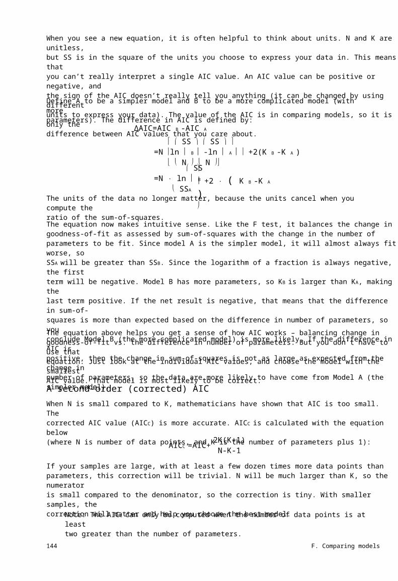
When you see a new equation, it is often helpful to think about units. N and K are unitless,but SS is in the square of the units you choose to express your data in. This means thatyou can’t really interpret a single AIC value. An AIC value can be positive or negative, andthe sign of the AIC doesn’t really tell you anything (it can be changed by using differentunits to express your data). The value of the AIC is in comparing models, so it is only thedifference between AIC values that you care about.

Define A to be a simpler model and B to be a more complicated model (with moreparameters). The difference in AIC is defined by:

∆AIC=AIC B -AIC A

SS SS =N ln B -ln A +2(K B -K A ) N N SS=N ⋅ ln B

SSA

+2 ⋅ ( K B -K A )

The units of the data no longer matter, because the units cancel when you compute theratio of the sum-of-squares.

The equation now makes intuitive sense. Like the F test, it balances the change ingoodness-of-fit as assessed by sum-of-squares with the change in the number ofparameters to be fit. Since model A is the simpler model, it will almost always fit worse, soSSA will be greater than SSB. Since the logarithm of a fraction is always negative, the firstterm will be negative. Model B has more parameters, so KB is larger than KA, making thelast term positive. If the net result is negative, that means that the difference in sum-of-squares is more than expected based on the difference in number of parameters, so youconclude Model B (the more complicated model) is more likely. If the difference in AIC ispositive, then the change in sum-of-squares is not as large as expected from the change innumber of parameters, so the data are more likely to have come from Model A (thesimpler model).

The equation above helps you get a sense of how AIC works – balancing change ingoodness-of-fit vs. the difference in number of parameters. But you don’t have to use thatequation. Just look at the individual AIC values, and choose the model with the smallestAIC value. That model is most likely to be correct.

A second-order (corrected) AICWhen N is small compared to K, mathematicians have shown that AIC is too small. Thecorrected AIC value (AICC) is more accurate. AICC is calculated with the equation below(where N is number of data points, and K is the number of parameters plus 1):

AICC =AIC+2K(K+1) N-K-1

If your samples are large, with at least a few dozen times more data points thanparameters, this correction will be trivial. N will be much larger than K, so the numeratoris small compared to the denominator, so the correction is tiny. With smaller samples, thecorrection will matter and help you choose the best model.

Note: The AICc can only be computed when the number of data points is at leasttwo greater than the number of parameters.


We recommend that you always use the AICc rather than the AIC. With small sample sizescommonly encountered in biological data analysis, the AICc is more accurate. With largesample sizes, the two values are very similar.

The change in AICc tells you the likelihood that a model is correctThe model with the lower AICc score is the model more likely to be correct. But how muchmore likely?

If the AICc scores are very close, there isn't much evidence to choose one model over theother. If the AICc scores are far apart, then the evidence is overwhelming. The probabilitythat you have chosen the correct model is computed by the following equation, where ∆ isthe difference between AICc scores.

probability= e-0.5∆1+e-0.5∆

Note: The probabilities are based on the difference between AICc scores. Theprobabilities are the same if the AICc scores are 620,000 and 620,010 as theyare if the AICc scores are 1 and 11. Only the absolute difference matters, not therelative difference.

This graph shows the relationship between the difference in AIC (or AICc) scores and theprobability that each model is true.

Percent chance that model A is correct

100%90%80%70%60%50%40%30%20%10%0%

-10 -9 -8 -7 -6 -5 -4 -3 -2 -1 0 1 2 3 4 5 6 7 8 9 10

0%

10%

20%

30%

40%

50%

60%

70%

80%

90%

100%

Percent chance that model B is correct

AICB - AICA

Note: These probabilities are also called Akaike’s weights.

If the two AICc values are the same, then the difference is zero, and each model is equallylikely to be correct. The graph shows that there is a 50% chance that model A is correct,and a 50% chance that model B is correct. If the difference is 2.0, with model A having thelower score, there is a 73% probability that model A is correct, and a 27% chance thatmodel B is correct. Another way to look at this is that model A is 73/27 or 2.7 times morelikely to be correct than model B. If the difference between AICc scores is 6.0, then model


A has a 95% chance of being correct so is 20 (95/5) times more likely to be correct thanmodel B.

Note: Akaike’s weights compute the relative probability of two models. It can beextended to compute the relative probabilities of a family of three or moremodels. But it is always possible that another model is even more likely. TheAICc method only compares the models you choose, and can’t tell you if adifferent model is more likely still.

The relative likelihood or evidence ratioWhen comparing two models, you can divide the probability that one model is correct bythe probability the other model is correct to obtain the evidence ratio, which is defined bythis equation.

Evidence Ratio=Probability that model 1 is correct1 = -0.5⋅∆AICc

Probability that model 2 is correct e

100000

10000

Evidence Ratio 1000

100

10

10 5 10 15 20

∆AICc

Note: The evidence ratio is based on the absolute difference between AICcscores, not the relative difference. You’ll get the same evidence ratio with AICcscores of 4567 and 4577 and AICc scores of 1 and 11. In both cases, thedifference is 10.

For example, if the AICc scores differ by 5.0, then the evidence ratio equals 12.18. Themodel with the lower AICc score is a bit more than twelve times more likely to be correctthan the other model. Most people don’t consider this to be completely persuasive. If thedifference in AICc scores equals 10, then the evidence ratio is 148, so the evidence isoverwhelmingly in favor of the model with the lower AICc.


Don’t overinterpret the evidence ratio. The ratio tells you the relative likelihood, givenyour experimental design, of the two models being correct. If you have few data points,the simpler model might fit best with a very high evidence ratio. This tells you that youcan be quite sure that the simple model is adequate to explain your data. With so fewpoints, you don’t have any real evidence that the more complicated model is right. Thisdoesn’t mean that a more complicated model might not explain your system better. If youhad lots of data, you might find that a more complicated model is more likely to becorrect.

Terminology to avoid when using AICc

The AIC is derived from information theory, which is different from statistical hypothesistesting. You can use the AICc method to determine the relative likelihood of two (or more)models. You can’t use AICc to decide whether the data fit “significantly” better to onemodel so you should “reject” the other. Therefore you should never use the terms“significant” or “reject” when presenting the conclusions of model comparison by AICc.These terms have very definite meanings in statistics that only apply when you compute aP value and use the construct of statistical hypothesis testing. Those terms carry too muchbaggage, so should only be used in the context of statistical hypothesis testing.

How to compare models with AICC by handEven if your nonlinear regression program does not compare models with the Akaike’sInformation Criteria, you can do so fairly simply. These steps review the equationspresented in this chapter, so you can compute AICc by hand.

1.

2.

Fit the first model using nonlinear regression.

Look at the results of nonlinear regression and write down the sum-of-squares;call this value SS. If you used any weighting factors, then record the weightedsum-of-squares.

Define N to be the number of data points. Be sure to account for replicatesproperly. If you have 13 X values with duplicate determinations of Y, and youasked the program to treat each replicate as a separate value, then N is 26.

Define K to be the number of parameters fit by nonlinear regression plus 1. Don’tcount parameters that are constrained to constant values. If in doubt, count thenumber of distinct SE values reported by nonlinear regression, then add 1 to getthe value of K. (Why add one? Because nonlinear regression is also “estimating”the value of the sum-of-squares.)

Compute AICC:

3.

4.

5.

2K(K+1) SS AICc =N ⋅ ln +2K+ N-K-1N

6.

7.

8.

Repeat steps 1-5 with the other model.

The model with the lower AICc score is more likely to be correct.

Calculate the evidence ratio from the difference in AICc scores:


Evidence Ratio=1

e -0.5⋅∆AICc

One-way ANOVA by AICcThe previous chapter showed how to turn one-way ANOVA into a model comparisonproblem, and did the comparison by the extra sum-of-squares F test. Here are the samedata, comparing models by AICc.

Model

Null hypothesis


SS

40.84

27.23

N

18

18

Pars

1

3

AICc

19.55

18.53

Probability

37.53%

62.47%

Evidence ratio

1.66

The alternative hypothesis (that the group means are not all identical) has the lower AICc.Thus, it is more likely to be correct than the null hypothesis that all the data come frompopulations with the same mean. But the evidence ratio is only 1.66. So the alternativehypothesis is more likely to be correct than the null hypothesis, but only 1.66 times morelikely. With so few data and so much scatter, you really don’t have enough evidence todecide between the two models.


24. How should you compare models -- AICc orF test?

A review of the approaches to comparing modelsChapter 21 discussed the general approach to use when comparing models. Mostimportant:

Before comparing models statistically, use common sense. Only use statisticalcomparisons to compare two models that make scientific sense, and where eachparameter has a sensible best-fit value and a reasonably narrow confidence interval. Manyscientists rush to look at statistical comparisons of models too soon. Take the time to askwhether each fit is sensible, and only rely on statistical comparisons when both models fitthe data well.

If you wish to compare two models that are not related (“nested”), then your only choice isto compare the fits with the AICc method. The F test should not be used to comparenonnested models. Since you’ll rarely find it helpful to compare fits of biological modelsthat are not nested, you’ll almost always compare nested models.

If the two models are related, and both fit the data with sensible parameter values, youcan choose between the F test and AIC method. The rest of this chapter explains theadvantages and disadvantages of the two approaches.

Pros and cons of using the F test to compare modelsThe F test is based on traditional statistical hypothesis testing.

The null hypothesis is that the simpler model (the one with fewer parameters) is correct.The improvement of the more complicated model is quantified as the difference in sum-of-squares. You expect some improvement just by chance, and the amount you expect bychance is determined by the number of degrees of freedom in each model. The F testcompares the difference in sum-of-squares with the difference you’d expect by chance.The result is expressed as the F ratio, from which a P value is calculated.

The P value answers this question: If the null hypothesis is really correct, in what fractionof experiments (the size of yours) will the difference in sum-of-squares be as large as youobserved or larger? If the P value is small, you’ll conclude that the simple model (the nullhypothesis) is wrong, and accept the more complicated model. Usually the threshold Pvalue is set at its traditional value of 0.05. If the P value is less than 0.05, then you rejectthe simpler (null) model and conclude that the more complicated model fits significantlybetter.

Reminder: The F test should only be used to compare two related (“nested”)models. If the two models are not nested, use the AICc method to comparethem.

24. How should you compare models -- AICc or F test? 149

The main advantage of the F test is familiarity. It uses the statistical hypothesis testingparadigm that will be familiar to the people who read your papers or attend yourpresentations. Many will even be familiar with the use of the F test to compare models.

The F test also has some disadvantages:

• You have to set an arbitrary value of alpha, the threshold P value belowwhich you deem the more complicated model to be “significantly” better so“reject” the simpler model. Traditionally, this value of alpha is set to 0.05,but this is arbitrary.

The value of alpha is generally set to the same value regardless of samplesize. This means that even if you did an experiment with many thousands ofdata points, there is a 5% chance of rejecting the simpler model even when itis correct. If you think about it, this doesn’t make much sense. As you collectmore and more data, you should be increasingly sure about which model iscorrect. It doesn’t really make sense to always allow a 5% chance of rejectingthe simple model falsely.

The F test cannot be readily extended to compare three or more models. Theproblem is one of interpreting multiple P values.

•

•

Pros and cons of using AICc to compare modelsThe AICc method is based on information theory, and does not use the traditional“hypothesis testing” statistical paradigm. Therefore it does not generate a P value, doesnot reach conclusions about “statistical significance”, and does not “reject” any model.

The AICc model determines how well the data supports each model. The model with thelowest AICc score is most likely to be correct. The difference in AICc score tells you howmuch more likely. Two models can be compared with a likelihood ratio, which tells youhow many times more likely one model is compared to the other.

The main advantage of the AIC approach is that it doesn’t tell you just which model ismore likely, it tells you how much more likely. This makes it much easier to interpret yourresults. If one model is hundreds or thousands of times more likely than another, you canmake a firm conclusion. If one model is only a few times more likely than the other, youcan only make a very tentative conclusion.

Another feature of the AIC approach (which we consider to be an advantage) is that themethod doesn’t make any decisions for you. It tells you which model is more likely to becorrect, and how much more likely. It is up to you to make a decision about whether toconclude that one model is clearly correct, or to conclude that the results are ambiguousand the experiment needs to be repeated. You can simply accept the more likely model.You can accept the simpler model unless the more complicated model is much morelikely. Or you can conclude that the data are ambiguous and make no decision aboutwhich model is best until you collect more data. This seems like a much more sensibleapproach to us than the rigid approach of statistical hypothesis testing.

A final advantage of the AICc approach is that it is easily extended to compare more thantwo models. Since you don’t set arbitrary values of alpha and declare “statisticalsignificance”, you don’t get trapped in the logical quandaries that accompany multiplestatistical comparisons.


The only real disadvantage of the AICc approach is that it is unfamiliar to many scientists.If you use this approach, you may have to explain the method as well as your data.

Which method should you use?When comparing models, by far the most important step comes before using either the Ftest or the AICc method. You should look at the graph of the fits and at the curve fittingresults. You should reject a model if one of the fits has best-fit values that make noscientific sense, if the confidence intervals for the parameters are extremely wide, or if atwo-phase (or two component) model fits with one phase having a tiny magnitude. Onlywhen both fits are sensible should you go on to compare the models statistically.

If you compare nonnested models, then the F test is not appropriate. Use the AICcapproach.

If you compare three or more models, then the whole approach of significance testing getstricky. Use the AICc approach.

In most cases, you’ll compare two nested models, so there is no clear advantage of oneapproach over the other. We prefer the AICc method for the reasons listed in the previoussection, mostly because AICc quantifies the strength of the evidence much better thandoes a P value. However, this is not a strong preference, and the F test method works welland has the advantage of familiarity.

Tip: Pick a method and stick with it. It is not appropriate to compare with bothmethods and pick the results that you like the best.

24. How should you compare models -- AICc or F test? 151

25. Examples of comparing the fit of two modelsto one data set

Example 1. Two-site competitive binding model clearly better.

The dataThe F test can compare two nested models. In this example, we compare a one-site to atwo-site competitive binding model.

log(Conc) -9.0 -8.5 -8.0 -7.5 -7.0 -6.5 -6.0 -5.5 -5.0 -4.5 -4.0

CPM3019289028252485209816781023 601 293 268 193

3000

CPM2000

1000

0

-9 -8 -7 -6 -5 -4log[inhibitor, M]

Do both fits make sense?The graph above shows the results of fitting both a one-site (dashed curve) and two-site(solid curve) competitive binding curve to some data. Here are the tabular results.

One site competitionBest-fit values BOTTOM TOP LOGEC50 EC50Std. Error BOTTOM TOP LOGEC5095% Confidence Intervals BOTTOM TOP LOGEC50 EC50Goodness of Fit Degrees of Freedom RІ Absolute Sum of Squares Sy.x

Two site competitionBest-fit values BOTTOM TOP FRACTION1 LOGEC50_1 LOGEC50_2 EC50_1 EC50_2Std. Error BOTTOM TOP FRACTION1 LOGEC50_1 LOGEC50_295% Confidence Intervals BOTTOM TOP FRACTION1 LOGEC50_1 LOGEC50_2 EC50_1 EC50_2Goodness of Fit Degrees of Freedom RІ Absolute Sum of Squares Sy.xConstraints FRACTION1

257.92873-6.4713.3814e-007

67.2766.120.07250

102.8 to 413.02721 to 3026-6.638 to -6.3042.3009e-007 to 4.9693e-007

80.9910116882120.9

188.87003030.0360.3130884-7.520541-6.1216393.016191e-0087.557197e-007

27.8855339.850590.057380870.19073650.07960846

120.6341 to 257.10592932.522 to 3127.5510.1726775 to 0.4534995-7.987273 to -7.053809-6.316442 to -5.9268371.029738e-008 to 8.834680e-0084.825679e-007 to 1.183484e-006

60.999194410475.9341.78503

0 < FRACTION1 < 1.000000

Look at the graph of the one site fit model (dashed curve). It seems to deviatesystematically from the data points, but not so badly that we will reject the modelcompletely. The graph of the two-site fit looks better. Do the best-fit values of the two-sitemodel make sense? The best-fit two-site curve has a high affinity site with a logEC50 of-7.5 comprising 31% of the sites, and a low affinity site with a logEC50 of -6.1. These resultsare certainly scientifically plausible. Next we look at the confidence intervals, which arereasonably narrow (given so few data points). Because the results are sensible, it makessense to compare the sum-of-squares statistically.

Compare with the F testThe F test compares the goodness-of-fit of the two models (assessed by the sum-of-squares, SS) adjusting for difference in the number of degrees of freedom (df).


Model SS dfNull hypothesis (1 site)

Alternative hypothesis (2 sites)

Difference

Fractional difference

Ratio (F)

116882

10476

106406

10.16

30.48

8

6

2

0.333

The two sum-of-squares values come from the nonlinear regression results.

The degrees of freedom equal the number of data points (11 in this example) minus thenumber of parameters fit by the program (three parameters for the one-site model, fivefor the two-site model).

Going from the two-site model to the one site model, the degrees of freedom increased33.3%. If the one-site model were correct, you'd expect the sum-of-squares to alsoincrease about 33.3% just by chance. In fact, the fit to the one-site model had a sum-of-squares 1016% higher than the fit to the two-site model. The relative increase in sum-of-squares was 30.5 times higher than the relative increase in degrees of freedom, so the Fratio is 30.5 with 2 (numerator) and 6 (denominator) degrees of freedom.

The P value is 0.0007. The P value is a probability, and it is easy to interpret. Start byassuming that the null hypothesis, the simpler one-site model, is really correct. Nowperform the experiment many times with the same number of data points, the same Xvalues, and the same amount of scatter (on average). Fit each experiment to both one- andtwo-site models. The two-site model will almost always fit the data better than the one-site model. But how much better? The P value is the fraction of those hypotheticalexperiments that you’d expect to find as a large a difference between the sum-of-squaresof the two-site model and one-site model as you actually observed.

You can’t know for sure which model is more appropriate for your data. All you can say isthat if the simpler (one-site) model were correct, it would be a very rare coincidence – onethat happens 0.07% of the time, or one time in 1428 experiments – to find data that fit thetwo-site model so well. Since that P value is lower than the traditional (but arbitrary)

25. Examples of comparing the fit of two models to one data set 153

threshold of 0.05, we’ll conclude that the two-site model fits the data significantly betterthan the one-site model.

Compare with AICc

Let’s compare the models using AICc. The sum-of-squares values come from the curve fit.There are 12 data points. The one-site model fits 3 parameters; the two-site model fits 5.Put these values into the equations presented in the previous chapter to calculate the AICcfor each model.

Model SS N Pars AICc Probability Evidence RatioOne site

Two site

116882

10476

11

11

3

5

116.65

108.45

1.63%

98.37%60.33

The two-site model has the lower AICc so is more likely to be correct. In fact, it is 98.37%certain to be correct, which means it is 60.33 times more likely to be correct than the one-site model.

Example 2: Two-site binding model doesn’t fit better.log(Conc)

-9.0-8.5-8.0-7.5-7.0-6.5-6.0-5.5-5.0-4.5-4.0

Y12849306228622731239820311369 761 503 401 279

CPM Y23009302429392830253318951252 631 580 186 350

Y32975294428662834252620391356 675 441 348 379

3000

2000

1000

0

-9 -8 -7 -6 -5 -4

CPM

log([inhibitor, M])

When you look at the graph of the results in this example (above), the two curves arealmost identical. You may even have difficulty seeing that the graph includes two curves.

Here are the tabular results of the two-site fit:


Best-fit values BOTTOM TOP FRACTION1 LOGEC50_1 LOGEC50_2 EC50_1 EC50_2Std. Error BOTTOM TOP FRACTION1 LOGEC50_1 LOGEC50_295% Confidence Intervals BOTTOM TOP FRACTION1 LOGEC50_1 LOGEC50_2 EC50_1 EC50_2Goodness of Fit Degrees of Freedom RІ Absolute Sum of Squares Sy.x

299.029860.1271-7.147-6.1457.1281e-0087.1579e-007

28.9733.220.16580.77400.1125

239.6 to 358.32918 to 30540.0 to 0.4667-8.732 to -5.562-6.376 to -5.9151.8530e-009 to 2.7420e-0064.2118e-007 to 1.2165e-006

280.996115025773.26

The two EC50 values are about a log apart. But the best-fit value for the fraction of highaffinity sites is only 13%, with a 95% confidence interval extending from 0 to 47%.

With such a wide confidence interval for the fraction of high-affinity sites, and with thetwo-site curve being barely distinguishable from the one-site curve, you should be dubiousabout the validity of the two-site fit. But those results are not nonsense, so we’ll pushahead and do the formal comparison with both the F test and the AICc method.

Here are the results of the comparison using the extra sum-of-squares F test:

Model SS dfNull hypothesis (1 site)

Alternative hypothesis (2 sites)

Difference


Ratio (F)

174334

150257

24077

0.1602

30

28

2

0.0714

2.24

The P value is 0.1248. If the one-site model were correct, and you performed manyexperiments like this one, you’d find that data fit a two-site model this much better than a

25. Examples of comparing the fit of two models to one data set 155

one-site model in about 12% of the experiments (about 1 in 8). Since the P value is higherthan the traditional threshold of 0.05, we conclude that we do not reject the nullhypothesis. The data do not fit a two-site model significantly better than they fit a one-sitemodel.

Here are the AICc calculations.

ModelOne site

Two site

SS174334

150257

N33

33

Pars3

5

AICc

290.88

289.98

Probability61.03 %

38.97 %

Evidence Ratio

1.57

The one-site model is more likely to be correct. But the evidence ratio is only 1.57. Withsuch a small evidence ratio, you can’t be very sure that the one-site model is right. Thedata are simply ambiguous.

Example 3. Can’t get a two-site binding model to fit at all.

log(Conc) Y12954295729772919259921721256 819 472 219 369

CPM Y22983292828942794280221551173 881 687 555 289

Y32942296529342852263322261304 832 510 228 327

3000

2000

1000

0

-9 -8 -7 -6 -5 -4

-9.0-8.5-8.0-7.5-7.0-6.5-6.0-5.5-5.0-4.5-4.0

CPM

log([inhibitor, M])

Here the data fit the one-site model just fine, resulting in the curve shown in the graph.

When we attempted to fit the data to a two-site model, the nonlinear regression programsaid “cannot converge”. We tried several sets of initial values for the parameters, but keptseeing that error message. The two-site model that we used was constrained such that theparameter Fraction, which determines the fraction of the high-affinity site, must have avalue between 0.0 and 1.0. When we lifted the constraint, the program was able to fit themodel, but with a best-fit value of fraction equal to -0.3. This makes no sense, so that fit isnonsense.

Since we can’t fit the data to a sensible two-site model, we accept the one-site model. Theproblems of fitting to a two-site model are not due to program bugs or invalid choices.Rather, the data simply don’t fit the two-site model, so it should be rejected. The problemswe had fitting the model provided useful information – that the data do not support thetwo-site model.


26. Testing whether a parameter differs from ahypothetical value

The approaches for comparing models described in the previous chapters can also be usedto perform statistical testing on individual model parameters. The key is to recast theproblem as a choice between two models, one where the parameter of interest isestimated, and another where the same model is refitted to the data with the parameter ofinterest constrained to a specified value. This concept is illustrated with an examplebelow.

Example. Is the Hill slope factor statistically different from 1.0?

log(Dose)

-9.0-8.5-8.0-7.5-7.0-6.5-6.0-5.5-5.0-4.5-4.0-3.5-3.0

ResponseY1Y2 5860 7161 4445 8058 7667 99 103132 130143 167161 163213 203189 210190 194203 189

200

Response150

100

50

0

10 -9 10 -8 10 -7 10 -6

Best-fit values BOTTOM TOP LOGEC50 HILLSLOPE EC50Std. Error BOTTOM TOP LOGEC50 HILLSLOPE

55.19199.9-5.9880.75351.0274e-006

5.5515.5990.11020.1356

10 -5 10 -4 10 -3

Dose (M)

Dose-response curves are defined by four parameters – the top plateau, the bottomplateau, the EC50 (the dose of drug that cause a response midway between top and bottomplateaus) and the slope factor, or Hill slope (which defines how steep the curve is). Whenthe response is closely coupled to occupancy of a receptor, you may expect the slope factorto equal 1.0.

In this example, we ask whether the Hill slope is significantly different from 1.0.

Compare models with the F testThe null hypothesis is that the standard Hill slope of 1.0 is correct. To fit the modelcorresponding to the null hypothesis (simpler model), you constrain the slope to equal1.0; you are thus fitting a three-parameter Hill equation (Top, Bottom, and LogEC50 beingestimated). The alternative hypothesis is that the Hill slope has some other value. To fitthis model, fit the variable slope sigmoidal dose-response curve equation (also called afour-parameter Hill equation). The program will find best-fit values of Top, Bottom,LogEC50 and HillSlope. For these data, the best-fit Hill slope is 0.7535. Is the differencebetween the fitted Hill slope value of 0.7535 and the hypothetical value of 1.0 more thanwe’d expect by chance?

Use the F test to find out.

26. Testing whether a parameter differs from a hypothetical value 157

Model SS dfNull hypothesis (Hill=1.0)

Alternative hypothesis (Hill unconstrained)

Difference


Ratio (F)

3504

3080

76

13.77%

3.03

23

22

1

4.55%

The data fit better (had a lower sum-of-squares) when the Hill slope was unconstrained.The program had one more way to adjust the curve to fit the data, so of course the sum-of-squares is better. In this example, the relative difference is 13.77%. The correspondingdifference in df is 4.55%.

The sum-of-squares increased relatively more than the degrees of freedom. The ratio ofthe two relative differences (13.77%/4.55%) is the F ratio, which equals 3.03. Allowing theprogram to find the best-fit value of the Hill slope led to a better fit than fixing it to thestandard value of 1.0. The improvement in goodness-of-fit was better than expected bychance, but only three times as good.

The P value is 0.0958. The P value tells us that we’d see this much improvement in sum-of-squares, or more, 9% of the time by chance alone if the true Hill slope really was 1.0.Since this is larger than the conventional cut-off of 5%, we conclude that fitting the Hillslope does not lead to a significantly better fit than fixing the Hill slope to theconventional value of 1.0. Our data do not provide us with convincing evidence to rejectthe null hypothesis that the Hill slope equals 1.0.

Compare models with AICc

We can also compare the models with AICc.

Model SS N Pars AICc Probability Evidence Ratio

Slope fixed to 1.0

Slope unconstrained

3504

3080

26

26

3

4

137.4

137.1

46.7%

53.3%1.11

The more complicated model (Hill slope fit to the data) has the lower AICc score, so it ismore likely to be correct. But the difference in AICc is small, so the evidence ratio is only1.11. With such a low ratio, you really can’t be at all sure which model will turn out to becorrect (if you repeated the experiment many times). All you can say is that the modelwith the slope free to vary is slightly more likely to be correct.

The AICc method does not follow the paradigm of statistical hypothesis testing. It is notdesigned to make a decision for you. Rather it tells you which model is more likely to becorrect, and how much more likely. For this example, the model with the variable Hillslope is more likely, but not much more likely. The best conclusion from these results is


that the data simply don’t define the Hill slope well enough to know whether it isindistinguishable from 1.0.

Compare with t testThere is an alternative approach that is sometimes used to test whether a parameter valuediffers significantly from a hypothetical value. You can test this using a one-sample t test.

The best-fit value of the Hill slope is 0.7535 with a standard error of 0.1356 (reported bythe nonlinear regression program). Calculate t using this equation:

t= Best-fit value-Hypothetical value 0.7535 − 1.00 == 1.816 SE0.1356

Determine a two-tailed P value for t=1.691 and 22 degrees of freedom (26 data pointsminus 4 parameters). Use a statistics table, the GraphPad QuickCalc web calculator, orthis Excel equation.

=TDIST(1.6816,22,2)

The P value is 0.1068. Since this is higher than the traditional cut-off of 0.05, youconclude that the Hill slope does not differ significantly from its standard value of 1.0.

This t test is only valid if two dubious assumptions are true:

• The distribution of the Hill slope is Gaussian. In other words, if you collected(or simulated) many data sets and fit each one, you are assuming that thedistribution of Hill Slopes would follow a Gaussian distribution. If it doesn’t,then the t test won’t be reliable and the P value won’t be exactly right.

The standard error of the Hill slope reported by the nonlinear regressionprogram is correct. In fact, nonlinear regression programs reportapproximate or asymptotic standard errors. In most cases, they are quiteaccurate. In some cases they are not.

•

Because these two assumptions may not be entirely appropriate, the P value obtainedfrom the t test is not exactly the same as the P value obtained from the F test. The F testassumes that the scatter of the data points around the curve follows a Gaussiandistribution. The t test only sees the Hill slope and its standard error, so it assumes thatthe Hill slope would follow a Gaussian distribution (if the experiment were repeated manytimes). This is a more dubious assumption.

We suggest that you avoid using the t test to compare parameter values. Instead use the Ftest (or AIC) to compare a model where the parameter’s value is fixed to a model wherethe parameter’s value is fit.

26. Testing whether a parameter differs from a hypothetical value 159

G. How does a treatment change the curve?

27. Using global fitting to test a treatment effectin one experiment

The logic underlying model comparisons described in the previous two chapters can alsobe extended to instances where you might want to compare one or more parameters of thesame model applied to different data sets. Some examples are shown below.

Does a treatment change the EC50?Below is a graph of a dose-response curve in control and treated conditions. We want toknow if the treatment changes the EC50. Are the two best-fit logEC50 values statisticallydifferent?

4000

Response3000

ControlTreated

2000

1000

010 -10 10 -9 10 -8 10 -7 10 -6 10 -5 10 -4 10 -3 10 -2

Dose (M)

One hypothesis is that both data sets have the same EC50. We fit that model by doing aglobal fit of both data sets. We fit two dose-response curves, while sharing the best-fitvalue of the logEC50. Fitting this model requires a program that can do global fits withshared parameters.

Here is the graph showing the curves with distinct top and bottom plateaus, distinct Hillslopes, but a single (shared) logEC50.

160 G. How does a treatment change the curve?

EC50

4000

Response3000

ControlTreated

2000

1000

010 -10 10 -9 10 -8 10 -7 10 -6 10 -5 10 -4 10 -3 10 -2

Dose (M)

The alternative hypothesis is that the EC50 values are distinct. We fit that model by fittingentirely separate dose-response curves to each data set. The two dotted lines show the twoEC50 values, which are quite close together.

Control EC50 Treated EC50

4000

Response3000

ControlTreated

2000

1000

010 -10 10 -9 10 -8 10 -7 10 -6 10 -5 10 -4 10 -3 10 -2

Dose (M)

Compare with F testHere is the comparison via the F test:

Model SS dfNull hypothesis (shared logEC50)

Alternative hypothesis (separate logEC50)

Difference

Relative difference

Ratio (F)

2,097,294

2,077,538

19,756

0.951%

0.42

45

44

1

2.273%

27. Using global fitting to test a treatment effect in one experiment 161

The relative change in SS is smaller than the relative change in df, so the P value must behigh. In fact, it is 0.52. If you performed many experiments where the treatment really didnot change the EC50, you’d find that the model with separate distinct logEC50 values fit thedata this much better (by chance) in 52% of the experiments. We conclude that there is nosignificant difference between logEC50 values.

Compare with AICc

Here is the comparison via AICc.

ModelShared logEC50

Separate logEC50

SS2,097,294

2,077,538

N52

52

K7

8

AICc

570.80

573.25

Probability77.25%

22.75%

Ratio

3.40

The model with a shared logEC50 has a lower AICc, so is more likely to be correct. But theshared model is only 3.40 times more likely to be correct than a model with separatelogEC50 values for each curve. Both models are supported by the data. The data are simplyambiguous.

Compare with t testIf your nonlinear regression program cannot fit models with shared parameters, you won’tbe able to use either the F test or the AICc approaches discussed above. Here is analternative approach that you can use. First let’s tabulate the best-fit value and SE fromeach data set when the data sets were fit separately.

Data setControl

Treated

Best-fit logEC50

-6.373

-6.295

SE0.07034

0.09266

df22

22

You can compare the two best-fit values for the logEC50 using a t test. It works much likethe unpaired t test for comparing means. The t ratio is calculated as:

t=logEC50control -logEC50treated

SE 2control +SE treated

2

= 0.078 =0.67 0.1163

You can find the associated P value using Excel. There are 44 degrees of freedom, and wewant a two-tailed P value.

=TDIST(0.67,44,2)

The P value is 0.51. The null hypothesis is that the two logEC50 values are really the same,and any discrepancy is due to random variation. If this null hypothesis were true, there isa 51% chance (the P value) of obtaining as large (or larger) a difference as you observed.Since this P value is so high, you conclude that there is no evidence to persuade you thatthe two logEC50 values are different. The preferred model is one with a shared logEC50.


This t test is only accurate if you assume that the value of the parameter follows aGaussian distribution (if you were to collect or simulate many data sets, and look at thedistribution of best-fit values). You must also assume that the standard errors of the best-fit values are accurate. Since these two assumptions can be dubious in some situations, wesuggest you avoid using the t test approach to compare data sets.

Does a treatment change the dose-response curve?Below is a graph of the same dose-response curves used in the previous example. We wantto know if the treatment does anything. Are the two curves statistically different?

4000

3000Response

ControlTreated

2000

1000

0

10 -10 10 -9 10 -8 10 -7 10 -6 10 -5 10 -4 10 -3 10 -2Dose (M)

In the previous example, we addressed this problem by focusing on a particular parameterof interest that we expected to be changed by the treatment (logEC50).

If you aren’t looking for a change in a particular parameter, you can recast the question toglobally compare two different data sets to the same model. We’ll compare the curves bycomparing two versions of the same model, the four-parameter Hill equation (often calledfour-parameter logistic equation).

The null hypothesis (first, simpler, model) is that one curve fits all the data points (bothdata sets) and the difference we see is purely due to chance. In essence, we ignore whichpoints are controls and which are treated, and fit a single curve to all the data and obtainone estimate for each of the four parameters in the model (Top, Bottom, logEC50 andHillSlope).

The easiest way to fit the null hypothesis is to constrain the four parameters so the valuesare shared between the two data sets.

GraphPad note: This is easy with Prism. Go to the constraints tab of thenonlinear regression dialog, and choose to make all four parameters shared.

If your computer program does not allow you to share parameters, you can still fit themodel. Enter all the values into one large data set, and then fit a single curve to thatcombined data set. Each experiment was performed with 13 doses and duplicatedetermination, so had 26 values. The combined data set, therefore, had twice that or 52values.


4000

Response3000

ControlTreated

2000

1000

010 -10 10 -9 10 -8 10 -7 10 -6 10 -5 10 -4 10 -3 10 -2

Dose (M)

The alternative model is that the curves are distinct. We fit each data set separately toobtain two distinct curves with four parameters for each data set.

To fit the alternative hypothesis, we separately fit the control data and treated data. Thesums-of-squares are 608,538 and 1,469,000, respectively. Add those two together to getthe sum-of-squares for the alternative hypothesis (which is 2,077,538). Each experimentwas performed with 13 doses and duplicate determination, so had 26 values. Sincenonlinear regression fit four parameters to each data set, each curve had 26-4, or 22degrees of freedom. Since the two fits are separate, the overall alternative model has22+22=44 degrees of freedom.

4000

Response3000

ControlTreated

2000

1000

010 -10 10 -9 10 -8 10 -7 10 -6 10 -5 10 -4 10 -3 10 -2

Dose (M)

Comparing with an F testThe models are nested, so it is appropriate to use the F test. Here are the results:


Model SS dfNull hypothesis (one curve for all data sets)

2,602,000

Alternative hypothesis (separate curves)

Difference

Relative difference

Ratio (F)

2,077,538

524,4462

25.24%

2.77

48

44

4

9.09%

The relative difference in SS was larger than the relative difference in df, so the F ratio isgreater than 1.0. For this example, F=2.77, with 4 and 44 degrees of freedom. Thecorresponding P value is 0.0386.

The P value is easy to interpret. If the treatment were entirely ineffective so the two dose-response curves are really identical, such a large a difference in the sum-of-squares (orlarger) would occur in only 3.86% of the experiments. Since this is less than thetraditional threshold of 5%, we reject the null hypothesis and conclude that the separate(not shared) fits are significantly better. The effect of the treatment on the dose-responserelationship was statistically significant.

Reality check: Look at the curves, which are very similar. In most experimental contexts,you wouldn’t care about such a small difference, even if you are sure that it is real and notdue to chance. Yes, the P value is small, so the difference is unlikely to be due to chance.But there is more to science than comparing P values with arbitrary thresholds to decidewhether something is “significant”.

Comparing with AICc

Here are the same data, compared with AICc.

ModelOne shared curve

Separate curves

SS2602000

2077538

N52

52

K4

8

AICc

573.97

573.25

Probability41.05%

58.95%

Ratio

1.44

The model with separate curves for each data set has the smaller AICc value, so it ispreferred. It is 1.44 times more likely to be correct than the simpler model with oneshared curve for both data sets. Because the evidence ratio is so low, we aren’t very sureabout the conclusion. If we repeated the experiment, it wouldn’t be surprising to find thatthe model with the shared curve was more likely.

Given the number of data points and the scatter, our data are simply ambiguous. Themodel with separate curves is more likely to be correct, so we’ll choose that model. But theevidence is not strong, so the conclusion is very weak.


28. Using two-way ANOVA to compare curves

Situations where curve fitting isn’t helpfulThe graph below shows a typical situation. You’ve measured a response at four timepoints, and compared control and treated conditions.

Control TreatedMean ± SD

100

Response75

50

25

0

Time

1234

Y1 45 65 89111

Control Y2Y3 4356 7169 9891 10098

Treated Y2Y3 5554 9276 104103 9390

Y1 49 87 99 87

1 2 3 4Time

You could fit to a simple model, say fit a straight line, but the response may not be linearwith time. You’d need some theory to help pick a model, but may not have any theoreticalreasons to pick a model. Even if you can pick a sensible model, you may have too few datapoints for nonlinear regression to work.

In this situation, many biologists analyze the data with two-way analysis of variance(ANOVA) as explained below.

Introduction to two-way ANOVATwo-way ANOVA, also called two-factor ANOVA, determines how a response is affectedby two distinct factors. For example, you might measure a response to three differentdrugs in both men and women. In this situation, two-way ANOVA partitions the overallvariability of the data into four parts:

•

•

•

166

Due to differences between men and women.

Due to differences among the three drugs.

Due to interaction. This is variation due to inconsistent differences betweenmen and women with different drugs.


• Due to random variability.

ANOVA compares the first three sources of variation with the amount of variation due torandom variability, and uses that to determine a P value. Thus it reports three different Pvalues testing three different null hypotheses.

The first null hypothesis is that there is no systematic difference between the differentlevels of the first factor. In this example, the null hypothesis is that there is no differencebetween the average result with men and woman, and any difference you see is due tochance. If this P value is low, you conclude that there is a significant difference.

The second null hypothesis is that there is no systematic difference between the levels ofthe second factor. In our example, the null hypothesis is that the average result is thesame with all three drugs, and that any difference you see is due to chance. If this P valueis small, you conclude that there is a significant variation among drugs.

The third null hypothesis is that the two factors don’t interact. In our example, thishypothesis is that any difference between men and women are the same for all threedrugs. Or equivalently, any difference among the drugs is the same for men and forwomen. If this P value is small, you reject this null hypothesis of no interaction.

How ANOVA can compare “curves”ANOVA analyzes data where the outcome (dependent variable) is a continuous variablesuch as enzyme activity, weight, or concentration. Each of the two factors is usuallycategorical, for example: male or female; drug A, B or C; or wild type or mutant. ANOVAis not usually used to assess the effects of a continuous variable, such as time or dose.Such data are usually analyzed by regression.

But in some situations, such as the one shown at the beginning of the chapter, you onlyhave collected data at a few time points or a few concentrations of a drug, and you reallycan’t use any curve-fitting procedure. An alternative is to use ANOVA, and treat the timepoints (or dosages) as if they were a categorical variable.

Two-way ANOVA partitions the overall variability of the data shown at the beginning ofthe chapter into four parts:

•

•

Due to differences between control and treated.

Due to differences among time points. Note that ANOVA treats different timepoints just like it would treat different drugs or different genotypes – there isno concept of trend.

Due to interaction. This is variation due to inconsistent differences betweencontrols and treated at different time points.

Due to random variability.

•

•

Here are the ANOVA results, showing how the variability is partitioned, along with thethree P values.

28. Using two-way ANOVA to compare curves 167

Source of Variation % of total variation P valueTreatment

Time

Interaction

Random

1.16

87.28

7.12

4.43

0.0572

P<0.0001

0.0013

The first P value is just above the traditional significance threshold of 5%. So the effect ofthe treatment does not appear to be statistically significant overall. The second P value istiny, so we reject the null hypothesis that time doesn’t matter. No surprise there. The thirdP value is also small. This tells us that there is a statistically significant interactionbetween treatment and time – the effect of the treatment is not consistent at all timepoints. Since this interaction is statistically significant, it makes sense to look further. Thisis done by performing Bonferroni post tests at each time point, as explained in the nextsection.

For completeness, here is the entire ANOVA table:

Source of VariationInteraction

Treatment

Time

Residual

df3

1

3

16

SS716.5

117.0

8782

446.0

MS238.8

117.0

2927

27.88

F8.568

4.199

105.0

Post-tests following two-way ANOVAThe Bonferroni post tests at each time point determine whether the difference betweencontrol and treated is statistically significant at each time point, and generate a 95%confidence interval for the difference between means at each time point. Here are theresults:

Time1

2

3

4

Difference4.667

16.67

9.33

-13.00

95% CI of diff.-7.460 to 16.79

4.540 to 28.79

-2.793 to 21.46

-25.13 to -0.8733

P valueP>0.05

P<0.01

P>0.05

P<0.05

The significance levels in the last column correct for multiple comparisons. The responseis significantly higher at time point 2, significantly lower at time point 4, and notsignificantly different at the other two time points.

If your program doesn’t perform the post-test automatically (Prism does), it is quite easyto calculate them by hand. The method we summarize below is detailed in pages 741-744

and 771 in J Neter, W Wasserman, and MH Kutner, Applied Linear Statistical Models, 3rdedition, Irwin, 1990.

For each time point or dose, calculate:

t=mean1 -mean 2

11 MSresidual + N1 N 2

The numerator is the difference between the mean response in the two data sets (usuallycontrol and treated) at a particular dose or time point. The denominator combines thenumber of replicates in the two groups at that dose with the mean square of the residuals(sometimes called the mean square of the error), which is a pooled measure of variabilityat all doses. Your ANOVA program will report this value, which it might call MSerror.

Statistical significance is determined by comparing the t ratio with a critical value from tdistribution, which we call t*. Its value depends on the number of df shown in the ANOVAtable for MSresidual, and on the number of comparisons you are making. You can get thecritical t value from Excel using the formula below, where DF is the number of degrees offreedom for the residual or error (as reported by the ANOVA program), Ncomparisons isthe number of comparisons you are making (usually equal to the number of time points ordoses in the analysis), and 0.05 is the significance level (traditionally set to 0.05, but youcould pick another value).

=TINV(0.05/Ncomparisons,DF)

For example data, there are four comparisons and 16 degrees of freedom (from theANOVA table for residual or error). Using Excel, t* equals 2.813

If a t ratio is higher than the threshold value computed by the Excel equation above, thenthe difference is statistically significant. If a t ratio is less than the threshold, then thatdifference is not statistically significant.

The equation for finding the critical value of t includes the Bonferroni correction bydividing the significance level (the P value that you consider to be significant, usually0.05) by the number of comparisons. This correction ensures that the 5% probabilityapplies to the entire family of comparisons, and not separately to each individualcomparison.

Confidence intervals are computed using this equation:

11 Span=t * ⋅ MSresidual + N1 N 2

95% CI: [ (mean 2 - mean1 ) - Span ] to [ (mean 2 - mean1 ) + Span ]The critical value of t is abbreviated t* in that equation (not a standard abbreviation). Itsvalue does not depend on your data, only on your experimental design. It depends on thenumber of degrees of freedom and the number of rows (number of comparisons) and canbe calculated using the Excel equation presented above.

Post-tests following repeated-measures two-way ANOVA use exactly the same equation ifthe repeated measures are by row. If the repeated measures are by column, use MSsubject

28. Using two-way ANOVA to compare curves 169

rather than MSresidual in both equations above, and use the degrees of freedom for subjects(matching) rather than the residual degrees of freedom.

The problem with using two-way ANOVA to compare curvesIt isn’t easy to make sense of the post-tests from our sample data. What does it mean thatyou get significant differences at time points 2 and 4, but not at time points 1 and 3? Thisis an intrinsic problem of this kind of analysis. Focusing on differences at particular timepoints (or doses) does not really address the scientific question you care about. It wouldbe better to compare rate constants, plateaus, area-under-the-curve, or some otherintegrated measure of the effect of the treatment. Asking about differences at individualtime points is not always helpful, and can lead to confusing results.

The fundamental problem is that the ANOVA calculations treat different time points (ordifferent doses) just like they treat different species, different genotypes, or differentcountries. ANOVA treats different time points, to use statistical lingo, as different levels ofa factor. The fact that the time points have an order is totally ignored. In fact, we’d getexactly the same two-way ANOVA results if we randomly scrambled the time points. Thefigure below rearranges the time points, yet the ANOVA results are identical.

100

Response75

50

25

0

Control TreatedMean ± SD

1 2 3 4Time

Two-way ANOVA can be a useful way to compare curves in some situations. But it rarelyanswers the questions you asked when you designed the experiment. Use this techniquewith caution.

Tip: Beware of using two-way ANOVA to analyze data where one of the factorsis time or dose. The ANOVA calculations ignore the concept of a trend. In otherwords, the ANOVA calculations ignore the entire point of the experiment.Whenever possible, use curve fitting rather than ANOVA.


29. Using a paired t test to test for a treatmenteffect in a series of matched experiments

The advantage of pooling data from several experimentsChapter 25 explained how to compare two curves obtained in one experiment. But if youreally want to know how a treatment changes the parameters of a curve, you’ll want torepeat the experiment several times. This chapter explains how to pool the results fromseveral experiments.

The first step is to focus on what you really want to know. In most cases, you’ll care mostabout a best-fit parameter from curve fitting. For example, with dose-response curves, youwill want to test whether the logEC50 is altered significantly by a treatment. With kineticcurves, you’ll ask about changes in the rate constant.

In some cases, you may wish to quantify the result in some other way rather than the best-fit value of a parameter determined by curve fitting. You may wish to tabulate themaximum response, the minimum response, or the time to maximum. Or you maytabulate the area under the curve as an overall measure of cumulative response. Sincethese values are not determined by nonlinear regression, you won’t be able to use themethods based on global fitting described in the next chapter. However, you may still usethe methods based on the t test.

An example. Does a treatment change logEC50? Pooling data fromthree experiments.Here is an example. We performed a dose-response experiment three times, each timebefore and after a treatment. To keep things simple (but not too unrealistic), all data werenormalized from 0 to 100, and we assumed that the slope would be standard (Hill slope=1). So we ask the program to fit only one parameter for each curve, the logEC50.

Here are the data:

And here is a graph of the data with a curves fit individually (six separate curve fits).

29. Using a paired t test to test for a treatment effect in a series of matched experiments 171

Experiment 1

100 100

Experiment 2

100

Experiment 3


Response50

0 ControlTreated

-9 -8 -7 -6 -5 -4 -3

0 ControlTreated

-9 -8 -7 -6 -5 -4 -3

0 ControlTreated

-9 -8 -7 -6 -5 -4 -3log(Dose) log(Dose) log(Dose)

Using the technique of Chapter 27, we can compare controls vs. treated in eachexperiment individually. For the first two experiments, this comparison yielded a P valueof less than 0.0001. For the third experiment, the P value is 0.0135. So in each experimentindividually, it is clear that the treatment significantly altered the logEC50.

Comparing via paired t testThe simplest approach to pooling the data is to perform a paired t test on the parameter ofinterest.

Note: As you’ll see in the next chapter, this approach is not the most powerfulway to analyze the data.

Before choosing any statistical test, you should always review its assumptions. The pairedt test assumes that your experiment was designed with the pairing in mind, that the pairsare independent, and that the distribution of differences between pairs (if you repeatedthe experiment many times) is Gaussian. These assumptions all seem reasonable for ourdata.

The figure below shows how the logEC50 values of our example are compared by paired ttest.

Paired t test-5.5 0.8 t=3.776 df=2

P=0.0635

Observed differencesMean: 0.376795%CI: -0.05252 to 0.8059

Change in log(EC 50)

0.70.60.50.40.30.20.10.0

log(EC50)-6.0

-6.5Control Treated Null hypothesis: Average change = 0

For this approach, only a single number was recorded for each experiment– the logEC50.The paired results are shown in the left panel above, as a before-after graph. The paired ttest works to simplify the data even more by subtracting the control logEC50 from thetreated logEC50. These differences are plotted in the right panel above. The paired t test iscomputed entirely from these three values. Divide the mean of these differences by thestandard error of the mean to compute the t ratio. To compute a P value, you have toknow the number of degrees of freedom. In a paired t test, the number of degrees offreedom equals the number of pairs minus 1. So in this experiment, there are two degrees


of freedom. From the t ratio and the number of df, you can find the P value using astatistical table or this Excel formula (the third parameter is 2 because you want a two-tailed P value):

=TDIST(3.776,2,2)

The result, the P value, is 0.0635. To interpret any P value, you need to state the nullhypothesis. Here, the null hypothesis is that the treatment has no effect so the meandifference is really zero. In other words, the null hypothesis is that individual animals areequally likely to have increases or decreases in the logEC50. If the null hypothesis weretrue, the chance of observing a mean difference as large or larger than we observed is justover 6%.

The P value of 0.06 is slightly higher than the traditional threshold of 0.05. Using thetraditional significance level, we would say that the difference observed in this set ofexperiments is not statistically significant. We do not have sufficient evidence to reject thenull hypothesis.

The mean difference between control and treated logEC50 is 0.3767.The 95% confidenceinterval for that difference extends from -0.05252 to 0.8059. These numbers are for thedifference between the logEC50 of control and the logEC50 in the treated group. Thedifference between two logarithms is the same as the logarithm of the ratio. So that value(0.3767) is also the log of the ratio of the treated EC50 divided by the control EC50. Takethe antilog, to convert to the ratio. The antilog (100.3767) is 2.381. So the treatmentincreases the EC50 by a factor of 2.4. Take the antilog of both ends of the confidenceinterval of the difference in logEC50 to express the confidence interval as a ratio. The 95%confidence interval for the ratio ranges from 0.8861 to 6.396. The 95% confidence intervalincludes 1 (no change), which is consistent with a P value greater than 0.05.

Why the paired t test results don’t agree with the individualcomparisonsWhen we analyzed each experiment independently, we found that the effect of thetreatment in each of the three experiments was statistically significant. In two of theexperiments, the P value was less than 0.0001. In the remaining experiment it was 0.017.

Now we pooled the three experiments using a paired t test, and the P value is 0.06. Thisdoesn’t make sense. The data in each experiment were sufficient to convince us that thetreatment worked. Put all three experiments together and now the data are not soconvincing. What’s wrong?

The problem is that the paired t test only takes into account best-fit values in eachexperiment. The paired t test doesn’t extend the method used to compare one pair ofcurves. Rather, it throws away most of the information, and only looks at the best-fit valuefrom each curve. The next chapter explains how to account for all the information in theseries of experiments.

29. Using a paired t test to test for a treatment effect in a series of matched experiments 173

30. Using global fitting to test for a treatmenteffect in a series of matched experiments

Why global fitting?The previous chapter used a paired t test to pool the results of three experiments. But theresults were not satisfying. When we compared treated with control for each experimentindividually, each P value was less than 0.05. With each individual experiment, theevidence is convincing. The effect of the treatment was statistically significant in each ofthe three experiments. But when we pooled all three experiments and analyzed with apaired t test, the result was not statistically significant.

The problem is that the paired t test analyzes only the best-fit values, in our example thelogEC50. It doesn’t take into account the other information in the experiment.

What we want is a method that extends the comparison we use to compare control andtreated groups in a single experiment to compare a family of experiments. Global curvefitting lets us do this.

Setting up the global modelHere is one way to write a global model that fits all the data and provides a best-fit valuefor the average treatment effect.

<A>logEC50=logEC50AEffect1 = MeanEffect + Rand1logEC50=logEC50A + Effect1

<C>logEC50=logEC50C<D>Effect2 = MeanEffect + Rand2<D>logEC50=logEC50C + Effect2

<E>logEC50=logEC50E<F>Effect3 = MeanEffect - Rand1 – Rand2<F>logEC50=logEC50E + Effect3

Y=100/(1+10^(LogEC50-X))

The last line in the model defines a sigmoidal dose-response curve that begins at 0, endsat 100, and has a standard Hill slope of 1.0. Therefore the equation defines Y as a functionof X and only one parameter, the log(EC50). However, we need to find a different logEC50for each data set. The rest of the model (the first nine lines) defines the logEC50 separatelyfor each of the six data sets.

The first line is preceded by “<A>” which (in GraphPad Prism) means it applies only todata set A. It defines the log(EC50) for that data set to be a parameter named logEC50A.(Because “logEC50” is used first on the left side of an equals sign, it is an intermediatevariable, and is not a parameter that Prism fits. Because “logEC50A” is used on the rightside of the equals sign, it is a parameter that Prism will fit.)

The second line defines the Effect (difference between logEC50 values) for the firstexperiment. It equals the mean treatment effect plus a random effect for that experiment,so we define the effect to equal MeanEffect + Rand1.

The third line defines the log(EC50) of data set B to equal the log(EC50) of data set A plusthe effect of the first experiment.

The next three lines define the second experiment (data sets C and D). This has a newcontrol value (logEC50C) and a different random effect (Rand2).

The final three lines define the third experiment (data sets E and F). Again there is a newcontrol value (logEC50E). The effect is defined a bit differently for this experiment, sinceit is the last. The effect is defined as the mean effect minus the random effects for the firsttwo experiments. Now if you average the effects for all three experiments, the randomeffects cancel out and the average effect really is the same as the parameter we callMeanEffect.

Average=( MeanEffect+Rand1) +(MeanEffect+Rand2)+(MeanEffect-Rand1-Rand2)

3=MeanEffect

If we wrote the model with three different random effects, the model would be ambiguous.It only requires three parameters (the mean effect, and two random effects) to completelydefine the three treatment effects.

The full model still has six parameters, as it must. Each experiment has only oneparameter, the logEC50, and there are six experiments. This model is written so there arethree logEC50 values for the controls, one parameter for the mean effect of the treatment,and two parameters that quantify how each experiment deviates from the average.

Fitting the model to our sample dataTo fit this model, we use global curve fitting, sharing the values of all six parameters. Thismeans we’ll fit one value for logEC50A that applies to data sets A (before) and B (after),one value of logEC50C value that applies to data sets C (before) and D (after), one valueof logEC50E value that applies to data sets E (before) and F (after), one MeanEffect valuethat applies to all three pairs of experiments, one value of Rand1 that applies toexperiments 1 and 3, and one value of Rand2 that applies to experiments 2 and 3.

Here are graphs of the resulting fits:

Experiment 1

100 100

Experiment 2

100

Experiment 3


Response50

0 ControlTreated

-9 -8 -7 -6 -5 -4 -3

0 ControlTreated

-9 -8 -7 -6 -5 -4 -3

0 ControlTreated


The sum-of-squares equals 7886 with 150 degrees of freedom. Why 150? There are 13concentrations, with Y values determined in duplicate, so there are 26 data points per

30. Using global fitting to test for a treatment effect in a series of matched experiments 175

curve. There are 6 curves, so there are 156 data points altogether. From that subtract thenumber of parameters we are fitting (6), resulting in 150 degrees of freedom.

The graphs are identical to fitting the data sets individually as shown in the previousChapter. This is what we expect since each of the three control curves has its own logEC50,and each of the three experiments has its own effect (difference between control andtreated). Rearranging the model to report the parameters arranged differently does notchange the appearance of the curves, the sum-of-squares, or the number of degrees offreedom.

Here are the results in tabular form:

Parameter Best-fit value SE 95% CILogEC50A

LogEC50C

LogEC50E

Rand1

Rand2

MeanEffect

-6.205

-6.154

-5.881

-0.01904

0.1812

0.3771

0.05852

0.05852

0.05852

0.06758

0.06758

0.04778

-6.320 to -6.090

-6.269 to -6.039

-5.996 to -5.767

-0.1515 to 0.1134

0.04879 to 0.3137

0.2835 to 0.4708

Interpreting the resultsThe best-fit value of MeanEffect is 0.3771. This is the same value calculated in the lastchapter when each curve was fit individually. But now we get a 95% confidence intervalbased on all the data in the experiment. We are 95% sure the treatment effect is between0.2835 to 0.4708. Because we are now fitting all the data, this confidence interval istighter (narrower) than the one we computed in the last chapter, which was based solelyon the three separate treatment effects.

The MeanEffect is the difference between the log(EC50) values. While that can be hard tointerpret, it is easy to convert to a form that is easier to understand. The differencebetween two logs is exactly the same as the logarithm of the ratio. So the MeanEffect is thelogarithm of the ratio of the two EC50 values. The antilog of the MeanEffect, which is 2.38,is the mean ratio of the EC50 for the treated divided by the EC50 of control. In other words,these data show that the treatment increased the EC50 by about a factor of two and a half.Now, take the antilog of both ends of the confidence interval of MeanEffect to obtain theconfidence interval of the fold change in EC50, which ranges from 1.921 to 2.957.

To summarize: We observed that the EC50 increased by a factor of about two and a half,and are 95% sure that change is somewhere between approximately a doubling andtripling.

Why are three standard errors of the logEC50 values all the same?

Note: This topic is here just to satisfy your curiosity. If you aren't curious, skipit!


Turn your attention to the standard errors of the best-fit parameters. Note that thestandard errors of all three logEC50 values are identical. If you display the results to moredecimal places, you’ll find they are not exactly identical. But they are very close.

To understand why these standard errors have values so close together, let’s review howthe standard errors of best-fit parameters are computed. The computation is complicatedand involves inverting a matrix, but depends on three terms:

• The sum-of-squares of the vertical distances of the data points from thecurves. In a global fit, it is the global (total) sum-of-squares that enters thecomputation. With six curves computed at once, this term is the sum of thesum-of-squares for each curve. There is only one sum-of-square value for allthe confidence intervals.

The number of degrees of freedom, computed as the number of data pointsminus the number of parameters. In a global fit, it uses the total number ofdata points and the total number of parameters. Therefore, there is only onedf value for all the confidence intervals.

A term that comes from the variance-covariance matrix. Its value isdetermined by computing how the Y value predicted by the model changeswhen you change the value of each parameter a little bit. More specifically, itsums the partial derivative of Y as a function of each parameter, holding theparameters equal to their best-fit value, at all values of X. The result dependson the model, the parameter, the number of data points, and the values of X.In our example, the three control curves all have the same number of datapoints, with the same X values. These X values are spaced so each data setcovers the bottom plateau, the middle, and the top of the curve. So this termis almost the same for all three curves.

•

•

The first two terms must be identical for all confidence intervals computed from a globalfit. The third term will vary between parameters, but will be almost identical betweenexperiments for a particular parameter (so long as the range of X values covers allimportant parts of the curve for all treatments). So it makes sense mathematically that thethree standard errors for logEC50 values would be nearly identical.

Does it make sense intuitively? Yes. Each experiment has the same number of data points.In each experiment, we have enough X values to define the top, middle, and bottom of thecurve. And it is reasonable to assume that the average amount of random scatter isidentical in all three experiments. Therefore, it makes sense that the logEC50 isdetermined with equal precision in each experiment. The global curve-fitting programeffectively averaged together the scatter for all three curves, to give one uncertainty valuethat applies to all three logEC50 values.

Was the treatment effective? Fitting the null hypothesis model.Was the treatment effective? Are we convinced that the treatment is real? One way toaddress this question is to look at the 95% confidence interval for the mean effect. Thisdid not include zero (no effect) so we are at least 95% sure the treatment did something.Looking at confidence intervals is a very good way to look at treatment effects, and onecould argue the best way. But it is more traditional to compute P values, so we'll do sohere.


To compute a P value (or use information theory and find the AICc), we need to comparetwo models. One model is that the control and treated logEC50 values are different – thetreatment worked. This model was explained in the previous section. The other model, thenull hypothesis, is that the treatment didn’t work, so the treated logEC50 values, onaverage, are identical to the control values.

We can fit the null hypothesis model using the same model as before, but constraining theMeanEffect parameter to be constant value of zero. Here are the graphs of theexperiments fit this way.

Experiment 1

100 100

Experiment 2

100

Experiment 3


Response50

0 ControlTreated

-9 -8 -7 -6 -5 -4 -3

0 ControlTreated

-9 -8 -7 -6 -5 -4 -3

0 ControlTreated


In the first experiment, the control and treated curves are almost identical, but they arenot identical in experiments 2 and 3. Our null hypothesis is not that control and treatedare identical in each experiment. Rather, the null hypothesis is that, on average, thecontrol and treated EC50 values are identical.

The curves don't follow the data very well. That is because we have constrained the meaneffect to equal zero.

Here are the results reported by nonlinear regression.

Parameter Best-fit value SE 95% CILogEC50A

LogEC50C

LogEC50E

Rand1

Rand2

MeanEffect

-6.007

-5.975

-5.682

-0.02808

0.2034

0.000

0.06361

0.06361

0.06362

0.08047

0.08047

(constant)

-6.131 to -5.882

-6.100 to -5.851

-5.806 to -5.557

-0.1858 to 0.1296

0.04572 to 0.3612

To check that these results are consistent with the null hypothesis, let's compute thetreatment effect in each experiment. In experiment 1, the model defines the treatmenteffect to equal the mean effect (which we now fix to zero) plus Rand1. So the treatmenteffect (difference between control and treated EC50 values) is -0.02808. For experiment2, the model defines the treatment effect to equal the mean effect plus Rand 2, which is0.2034. For experiment 3, the model defines the treatment effect to equal the mean effectminus the sum of Rand1 and Rand2, which is -0.17532. So the average effect of the


treatment in all three experiments is (-0.02808 +0.2034 -0.17532)/3, which equals zeroas it must under the null hypothesis.

Again, the standard errors are all the same. We fit all three experiments in one global fit.Since we are fitting the same model to experiments with the same number of data pointsand same X values, all the SE values are the same.

The total sum-of-squares equals 11257 with 151 degrees of freedom. Why 151? There are 13concentrations, with Y values determined in duplicate, so there are 26 data points percurve. There are 6 curves, so there are 156 data points altogether. From that subtract thenumber of parameters we are fitting (5), resulting in 151 degrees of freedom.

Comparing models with an F testWe used global fitting to fit the data to two models. One assumes the treatment worked.The other (the null hypothesis) constrained the mean treatment to equal zero.

Here are the calculations of an F test to compare the two models.

Model SS dfNull hypothesis (treatment effects arezero)

Alternative hypothesis (treatment notzero)

Difference

Relative difference

Ratio (F)

11257

7886

3371

0.4275

64.12

151

150

1

0.67

With such a high F ratio, the P value is tiny, way less than 0.0001. If the null hypothesiswere true (that all treatment effects were really zero), there is only a slim chance (way lessthan 0.01%) of seeing such large treatment effects in a series of three experiments of thissize. In other words, it is exceedingly unlikely that the difference we observed betweencontrol and treated dose-response curves is due to chance.

We conclude that the treatment effects are statistically significant, extremely so.

Comparing models with AICc

Alternatively, here are the results analyzed by AICc.

ModelTreatment has no effect

Treatment is effective

SS11257

7886

N156

156

K5

6

AICc Probability<0.01%

>99.99%3.8x1011

Ratio680.07

626.74

The AICc for the second model (treatment does have an effect) is much lower, so thismodel is much more likely to be true. In fact, given our data and these two alternatives,

the second model is many billions times more likely to be correct. We have substantialevidence that the treatment altered the logEC50 in our series of three experiments.

Reality checkThe result of this set of experiments convinces us that the treatment effect is not zero.Rather, we are fairly sure the treatment effect is somewhere between a doubling andtripling of the EC50. Statistically, we are convinced this is distinct from zero. We are quitesure the treatment did something -- the difference we observed is extremely unlikely to bedue to random chance. In other words, we can say the results are statistically significant.

You should always interpret results in the context of the experiment. Do you care about adoubling or tripling of an EC50? In some contexts, this would be considered a small, trivialeffect not worth pursuing. Those judgments cannot be made by statistical calculations. Itdepends on why you did the experiment. Statistical calculations can tell us that the effectis very unlikely to be due to chance. This does not mean it is large enough to bescientifically interesting or worth reporting.


31. Using an unpaired t test to test for atreatment effect in a series of unmatchedexperiments

An exampleWe measured enzyme velocity as a function of substrate concentration in the presenceand absence of a treatment. We had three control animals and three treated. We obtainedtissue from each, and measured enzyme activity at various concentrations of substrate. Allsix curves were obtained at one time, with no pairing or matching between particularcontrol and treated animals.

Control3000 3000

Treated

Enzyme Velocity2000

Enzyme Velocity

0 25 50 75 100 125 150

2000

1000 1000

0 00 25 50 75 100 125 150

[Substrate] [Substrate]

Fitting the curves individually yields these results.

A:Control B:Control C:Control D:Treated E:Treated F:TreatedVMAX

Km

2190

14.10

2132

22.42

2428

17.04

2897

20.73

2449

16.64

2689

21.96

Using the unpaired t test to compare best-fit values of Vmax

Conceptually the easiest way to analyze the data is to use an unpaired t test. The graphbelow shows the six Vmax values, along with the results of the unpaired t test.

3000

Vmax2000

∆ = 428.495% CI: -10.02 to 866.8

1000 P= 0.0534

0Control Treated

31. Using an unpaired t test to test for a treatment effect in a series of unmatched experiments 181

The P value is just above the traditional threshold of 0.05, so the difference is said to notbe statistically significant. If the treatment did nothing to the Vmax of the enzyme, and yourepeated this kind of experiment many times (each time with the same doses, the sameaverage amount of scatter, and with three animals in each group), you’d find this largedifference (or larger) in a bit more than 5% of the experiments.

The confidence interval for the mean difference between control and treated Vmax rangesfrom a decrease of 10 to an increase of 867. This confidence interval spans zero, as it mustto be consistent with a P value greater than 0.05.

This t test tells you that the evidence is not strong enough to persuade you that thetreatment changes Vmax. But the results do look intriguing.

The problem with the t test is that it analyzes only the best-fit value of the parameter ofinterest. It doesn’t look at all the data in the experiment. To take into account all the data,we need to use global fitting as explained in the next chapter.


32. Using global fitting to test for a treatmenteffect in a series of unmatched experiments

Setting up a global fitting to analyze unpaired experimentsLet’s continue the example from the previous chapter.

Here is the model to fit the data with global fitting. It uses the syntax of GraphPad Prism.

<A>Vmax = MeanCon + Rand1Vmax = MeanCon + Rand2<C>Vmax = MeanCon - Rand1 - Rand2

<D>Vmax = MeanCon + Effect + RandT1<E>Vmax = MeanCon + Effect + RandT2<F>Vmax = MeanCon + Effect - RandT1 - RandT2

Y=Vmax*X/(Kd+X)

The bottom line in the model defines the enzyme kinetics curve.

The first six lines in the model define the Vmax term for each data set. Data sets A, B, and Cwere controls. We want to fit the mean Vmax for the control curves. Curve A has a Vmaxdefined to be equal to the mean value for the control (MeanCon) plus a random factor(Rand1). Curve B is defined similarly with a different random factor. Curve C is defined asthe mean control value minus the two random factors. If you take the average of the threeVmax values for curves A, B and C, you’ll see that the average really is MeanCon.

Average=( MeanCon+Rand1) + ( MeanCon+Rand2 ) + ( MeanCon-Rand1-Rand2 )

3=MeanCon

Curves D, E, and F are for the treated condition. The mean of the treated is defined to bethe mean of the controls plus a variable called Effect. This is the difference between themean of the controls and the mean of the treated. The variation around this mean ismodeled by RandT1 and RandT2.

The model looks complicated, but it needs to be that way to fit a single parameter, Effect,for the mean difference between the control and treated animals. The model has sevenparameters to fit: Km, MeanCon, Rand1, Rand2, Effect, RandT1, and RandT2.

When fitting this model, all the parameters that define the Vmax and the treatment effectmust be shared. But what about Km? You could argue that it should be shared, since thereis no evidence that the treatment changes the Km, and no theory suggesting it might. Oryou could argue that the Km might really vary between animals based on subtle differencesin the pH or ionic composition of the preparations. We chose the latter approach,although the results below would be very similar if we had designated the Km to be ashared parameter.

32. Using global fitting to test for a treatment effect in a series of unmatched experiments 183

Fitting our sample data to the global modelWe fit the data using global curve fitting, sharing all parameters except the Km. Here arethe results for the other parameters. Since they are shared, we get one best-fit value foreach for the entire model.

Parameter Best-fit value SE 95% CIMeanCon

RandC1

RandC2

Effect

RandT1

RandT2

2250.00

-60.27

-118.10

428.30

218.40

-228.90

65.50

87.15

99.17

95.26

99.07

93.29

2119 to 2381

-234.2 to 113.7

-316.1 to 79.81

238.2 to 618.5

20.62 to 416.1

-415.1 to -42.74

The first thing to do is make sure that the results match the results of the individual fits.This is a way to make sure that the model is correct. The Vmax for the first data set (A) isdefined as MeanCon+Rand1, or 2250 – 60.27, which equals (to four digits of precision)2190. This is identical to the value we obtained when we fit each curve independently.Similarly, the other Vmax values all match the values obtained when we fit the curvesindependently. Using the global model did not change the best-fit curves, just how weorganize the results. The sum-of-squares (1145088) of the global fit accordingly matchesthe sum of the sum-of-squares of the six individual curve fits. Similarly, the degrees offreedom of the global fit (72) match the sum of the degrees of freedom of the sixindividual curves.

The whole point of this fit is to determine the best-fit value of the treatment effect. Thebest-fit value is 428. This is the same as the mean difference we calculated for theunpaired t test. No surprise here. The curves are the same, so the difference between theaverage control Vmax and the average treated Vmax has to match. If it didn’t, we know therewas something wrong with how we set up or fit the global model.

Now let’s turn our attention to the confidence interval of the treatment effect. The globalfit tells us that we can be 95% sure that the range 228 to 619 contains the true treatmenteffect. This interval was calculated by considering all of our data. In contrast, the t testonly took into account the six Vmax values so its confidence interval was much wider (-10 to867).

Finally, let’s compute a P value testing the null hypothesis that the treatment reallydoesn’t affect the Vmax at all. To do this, we compare the fit we just did with oneconstrained so Effect=0. Here are the results.

Parameter Best-fit value SE 95% CIMeanCon

RandC1

RandC2

184

2505

-164.5

28.20

55.15

110.4

137.8

2395 to 2615

-384.9 to 55.79

-246.9 to 303.3


Effect

RandT1

RandT2

0.0 (fixed)

206.4

-200.7

100.3

94.83

6.248 to 406.5

-390.0 to -11.49

Let’s check that this fit makes sense.

Parameter

Control A

Control B

Control C

Treated D

Treated E

Treated F

Calculation

2505 - 165

2505 + 28

2505 + 165 - 28

2505 + 206

2505 - 201

2505 – 206 + 201

Value

2340

2533

2642

2711

2304

2500

2505

2505

Mean

Each curve is fit its own Vmax value, but the global fitting was constructed to ensure thatthe average of the control Vmax values matched the average of the treated Vmax values(since Effect was constrained to equal 0). The table shows that the fit worked as intended.The two means are the same.

Comparing models with an F testHere are the calculations of an F test to compare the two models.

Model

Null hypothesis (treatment effect is zero)

Alternative hypothesis (treatment notzero)

Difference

Relative difference

Ratio (F)

SS

1,442,275

1,145,087

297,188

0.25953

18.68

df

73

72

1

0.01389

With such a high F ratio, the P value is tiny, much less than 0.0001. If the null hypothesis(that the treatment doesn’t change Vmax) were true, there is only a slim chance (way lessthan 0.01%) of seeing such large treatment effects in our series of six experiments. Inother words, it is exceedingly unlikely that the difference we observed between controland treated Vmax is due to chance.

32. Using global fitting to test for a treatment effect in a series of unmatched experiments 185

We conclude that the treatment effect is statistically significant.

Comparing models with AICc

Here are the results analyzed by AICc.

ModelTreatment hasno effect

Treatment iseffective

SS1,442,275

1,145,087

N84

84

K11

12

AICc847.5

830.9

Probability0.03%

99.97%3977

Ratio

The AICc for the second model (treatment does have an effect) is much lower, so thismodel is much more likely to be true. In fact, given our data and these two alternatives,the second model is almost four thousand times more likely to be correct. We havesubstantial evidence that the treatment altered the Vmax in our series of experiments.

Reality checkThe global fit convinced us that the difference we observed in Vmax between control andtreated animals is very unlikely to be due to chance. The P value is tiny, so the results arestatistically significant. The AICc criterion tells us that a model where control and treatedhave the same average Vmax is extremely unlikely to be correct.

When interpreting data, one should not focus on statistical significance. Instead,concentrate on the size of the difference. Our treatment effect was 428, compared tocontrol mean of 2228. This means the treatment increased Vmax, on average, by 428/2228or only 19.2%. Putting aside statistical calculations of P values, you cannot really interpretthese results except by thinking about the reason you did the experiment. Is a 20% changeworth caring about? The answer depends on why you did the experiment.


H. Fitting radioligand and enzyme kineticsdata

33. The law of mass action

What is the law of mass action?Analyses of radioligand binding experiments and enzyme kinetics are based on a simplemolecular model called the law of mass action. This “law” states that the velocity of achemical reaction is proportional to the product of the concentrations (or mass) of thereactants.

In the simplest case, one kind of molecule is transformed into a different kind of molecule.The rate at which the reaction occurs is proportional to the concentration of the startingmaterial.

A→ZdA dZ =- =k ⋅ [ A ]dtdt

If two molecules combine, the reaction rate is proportional to the product of theconcentrations.

A+B → ZdZ dA dB =-=-=k ⋅ [ A ] ⋅ [ B]dtdtdt

If a molecule dimerizes, the reaction rate is proportional to the square of itsconcentration.

A+A → ZdZ = k ⋅ [ A ] ⋅ [ A ] = k ⋅ [A]2

dt

The law of mass action applied to receptor bindingBinding between a ligand and its receptor is described by a simple, reversible, bimolecularreaction. (“Ligand” is just a fancy word for a molecule that binds to something.)

Receptor + LigandKon→

←Koff

Receptor ⋅ Ligand

According to the law of mass action, the rate of association is:

33. The law of mass action 187

Number of binding events per unit of time = kon⋅ [Ligand]⋅[Receptor].

[Ligand] and [Receptor] represent the free (not total) concentrations of each reactant,respectively, and kon denotes the association rate constant.

The law of mass action says that the reverse reaction (the dissociation of the complex)occurs at a rate proportional to the concentration of the complex.

Number of dissociation events per unit time = [Ligand⋅Receptor]⋅koff.

Here koff is the dissociation rate constant, in units of inverse time.

You can also make sense of these equations intuitively. Forward binding occurs whenligand and receptor collide due to diffusion, so the rate of binding is proportional to theconcentration of each. The rate constant takes into account the fact that not everycollision leads to binding -- the collision must have the correct orientation and enoughenergy. Once binding has occurred, the ligand and receptor remain bound together for arandom amount of time. The probability of dissociation is the same at every instant oftime. Therefore the rate of dissociation is only proportional to the concentration of thereceptor ligand complex.

After dissociation, the ligand and receptor are the same as they were before binding. Ifeither the ligand or receptor is chemically modified, then the binding does not follow thelaw of mass action.

Mass action model at equilibriumEquilibrium is reached when the rate at which new ligand⋅receptor complexes are formedequals the rate at which the ligand⋅receptor complexes dissociate. At equilibrium:

[ Ligand ] ⋅ [ Receptor ] ⋅ k on = [ Ligand ⋅ Receptor ] ⋅ k off

Rearrange that equation to define the equilibrium dissociation constant Kd.

[ Ligand ] ⋅ [ Receptor ] = k off

[ Ligand ⋅ Receptor ] k on= Kd

The Kd has a meaning that is easy to understand. Set [Ligand] equal to Kd in the equationabove. The Kd terms cancel out, and you'll see that the ratio [Receptor]/[Ligand⋅Receptor] equals 1.0, so [Receptor] equals [Ligand⋅Receptor]. Since all thereceptors are either free or bound to ligand, this means that half the receptors are free andhalf are bound to ligand. In other words, when the concentration of ligand equals the Kd,at equilibrium ligand will be bound to half the receptors.

If the receptors have a high affinity for the ligand, even a low concentration of ligand willbind a substantial number of receptors, so the the Kd will be low. If the receptors have alower affinity for the ligand, you’ll need more ligand to get binding, so the Kd will be high.

Don’t mix up Kd, the equilibrium dissociation constant, with koff, the dissociation rateconstant. Even though they both include the word “dissociation”, they are not the same,and aren't even expressed in the same units.

The table below reviews the units used to express the rate and equilibrium constants.

188 H. Fitting radioligand and enzyme kinetics data

Constantkon

koff

Kd

NameAssociation rate constant, or on-rateconstant

Dissociation rate constant, or off-rateconstant

Equilibrium dissociation constant

UnitsM-1min-1 (or M-1sec-1)

min-1 (or sec-1)

M

Fractional occupancy predicted by the law of mass action atequilibriumThe law of mass action predicts the fractional receptor occupancy at equilibrium as afunction of ligand concentration. Fractional occupancy is the fraction of all receptors thatare bound to ligand.

Fractional occupancy= [Ligand ⋅ Receptor] [Total Receptor] [Ligand ⋅ Receptor]= [Receptor]+[Ligand ⋅ Receptor]

This equation is not useful because you don’t know the concentration of unoccupiedreceptor, [Receptor]. A bit of algebra creates a useful equation. First, rearrange thedefinition of the Kd.

[ Ligand ] ⋅ [ Receptor ] [ Ligand ⋅ Receptor ] [ Ligand ] ⋅ [ Receptor ][ Ligand ⋅ Receptor ] =

Kd =

Kd

Now substitute that expression for [Ligand.Receptor] in the equation that definesfractional occupancy.

Fractional occupancy= [Ligand ⋅ Receptor] [Receptor]+[Ligand ⋅ Receptor] [Ligand] ⋅ [Receptor]/K d

== [Receptor]+ ([Ligand] ⋅ [Receptor]/K d )

[Ligand][Ligand+K d ]=

This equation assumes equilibrium. To make sense of it, think about a few different valuesfor [Ligand].


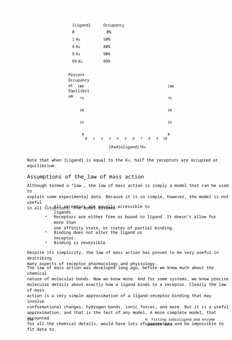
[Ligand]0

1.Kd

4.Kd

9.Kd

99.Kd

Percent Occupancy at Equilibrium

Occupancy0%

50%

80%

90%

99%

100

75

50

25

00 1 2 3 4 5 6 7 8 9 10

100

75

50

25

0

[Radioligand]/Kd

Note that when [Ligand] is equal to the Kd, half the receptors are occupied at equilibrium.

Assumptions of the law of mass actionAlthough termed a “law”, the law of mass action is simply a model that can be used toexplain some experimental data. Because it is so simple, however, the model is not usefulin all situations. The model assumes:

•

•

•

•

All receptors are equally accessible to ligands.

Receptors are either free or bound to ligand. It doesn’t allow for more thanone affinity state, or states of partial binding.

Binding does not alter the ligand or receptor.

Binding is reversible.

Despite its simplicity, the law of mass action has proven to be very useful in describingmany aspects of receptor pharmacology and physiology.

The law of mass action was developed long ago, before we knew much about the chemicalnature of molecular bonds. Now we know more. And for some systems, we know precisemolecular details about exactly how a ligand binds to a receptor. Clearly the law of massaction is a very simple approximation of a ligand-receptor binding that may involveconformational changes, hydrogen bonds, ionic forces, and more. But it is a usefulapproximation, and that is the test of any model. A more complete model, that accountedfor all the chemical details, would have lots of parameters and be impossible to fit data to.


Hyperbolas, isotherms, and sigmoidal curvesThe graphs below show binding at equilibrium, as predicted by the law of mass action.The two graphs show the same thing, but have different shapes.

• The graph on the left plots occupancy as a function of [Ligand]. It follows amathematical form called a rectangular hyperbola, which is also called abinding isotherm.

The graph on the right plots occupancy as a function of the logarithm of[Ligand] (or equivalently, plots occupancy as a function of [Ligand] plottedon a logarithmic axis). This graph follows a sigmoidal shape. The solidportion of this curve corresponds to the curve on the left. The dotted portionof the curve goes to higher concentrations of [Ligand] not shown on the othergraph.

100%

•

Occupancy at Equilibrium

Occupancy at equilibrium

100%

75%

50%

25%

0% 0.01

75%

50%

25%

0%0 1 2 3 4 5 6 7 8 9 10 0.1 1 10 100

[Ligand]/K d [Ligand]/K d


34. Analyzing radioligand binding data

Introduction to radioligand bindingA radioligand is a radioactively labeled drug that can associate with a receptor,transporter, enzyme, or any site of interest. Measuring the rate and extent of bindingprovides information on the number of binding sites, and their affinity and accessibilityfor various drugs. There are three kinds of experimental protocols for radioligand binding,discussed in the next three chapters.

Saturation binding experiments measure equilibrium binding of variousconcentrations of the radioligand. Analyze the relationship between binding and ligandconcentration to determine the number of sites, Bmax, and the ligand affinity, Kd. See"Analyzing saturation radioligand binding data" on page 199.

Competitive binding experiments measure equilibrium binding of a singleconcentration of radioligand at various concentrations of an unlabeled competitor.Analyze these data to learn the affinity of the receptor for the competitor. See "Analyzingcompetitive binding data" on page 211.

Kinetic experiments measure binding at various times to determine the rate constantsfor radioligand association and dissociation. See "Analyzing kinetic binding data" on page233.

Nonspecific bindingIn addition to binding to receptors of interest, radioligands also bind to other sites.Binding to the receptor of interest is called specific binding, while binding to the othersites is called nonspecific binding. This means that nonspecific binding can representseveral phenomena:

• In most cases, the bulk of nonspecific binding represents some sort ofinteraction of the ligand with membranes. The molecular details are unclear,but nonspecific binding depends on the charge and hydrophobicity of aligand – but not its exact structure.

Nonspecific binding can also be binding to receptors, transporters, or otherproteins not of interest to the investigator. For example binding of theadrenoceptor agonist, epinephrine, to serotonin receptors or metabolicenzymes can be considered “nonspecific”.

Nonspecific binding can also be binding to the filters used to separate boundfrom free ligand.

•

•

Nonspecific binding is usually (but not necessarily) proportional to the concentration ofradioligand (within the range it is used). Add twice as much radioligand, and you'll seetwice as much nonspecific binding.

Nonspecific binding is detected by measuring radioligand binding in the presence of asaturating concentration of an unlabeled drug that binds to the receptors. Under those


conditions, virtually all the receptors are occupied by the unlabeled drug so theradioligand can only bind to nonspecific sites. Subtract the nonspecific binding at aparticular concentration of radioligand from the total binding at that concentration tocalculate the specific radioligand binding to receptors.

Which unlabeled drug should you use for determining nonspecific binding? The obviousanswer is to use the same compound as the radioligand, but in its unlabeled form. Inmany cases this is necessary, as no other drug is known to bind to the receptors. But mostinvestigators avoid using the same compound as the hot and cold ligand and prefer todefine nonspecific binding with a drug that is chemically distinct from the radioligand butwhich binds to the same receptor.

What concentration of unlabeled drug should you use? You want to use enough to blockvirtually all the specific radioligand binding, but not so much that you cause more generalphysical changes to the membrane that might alter binding. If you are studying a well-characterized receptor, a useful rule-of-thumb is to use the unlabeled compound at aconcentration equal to 100 times its Kd for the receptors, or 100 times the highestconcentration of radioligand, whichever is higher.

Ideally, you should get the same results defining nonspecific binding with a range ofconcentrations of several drugs, and you should test this when possible. In many assaysystems, nonspecific binding is only 10-20% of the total radioligand binding. If thenonspecific binding makes up more than half of the total binding, you'll find it hard to getquality data. If your system has a lot of nonspecific binding, try different kinds of filters, alarger volume of washing buffer, warmer washing buffer, or a different radioligand.

Ligand depletionIn many experimental situations, you can assume that a very small fraction of the ligandbinds to receptors (or to nonspecific sites). In these situations, you can also assume thatthe free concentration of ligand is approximately equal to the concentration you added.This assumption vastly simplifies the analysis of binding experiments, and the standardanalysis methods depend on this assumption.

In other situations, a large fraction of the ligand binds to the receptors (or bindsnonspecifically). This means that the concentration of ligand free in the solution does notequal the concentration you added. The discrepancy is not the same in all tubes or at alltimes. The free ligand concentration is depleted by binding.

Many investigators use this rule of thumb: If less than 10% of the ligand binds, don'tworry about ligand depletion; if more than 10% of the ligand binds, you have threechoices:

• Change the experimental conditions. Increase the reaction volume withoutchanging the amount of tissue. The problem with this approach is that itrequires more radioligand, which is usually very expensive.

Measure the free concentration of ligand in every tube. This is possible if youuse centrifugation or equilibrium dialysis, but is quite difficult if you usevacuum filtration to remove free radioligand.

Use analysis techniques that adjust for the difference between theconcentration of added ligand and the concentration of free ligand. The nextfew chapters explain several such methods.

193

•

•

34. Analyzing radioligand binding data

35. Calculations with radioactivity

Efficiency of detecting radioactivityIt is not possible to detect each radioactive disintegration. The fraction of radioactivedisintegrations detected by your counter is called efficiency. Determine efficiency bycounting a standard sample under conditions identical to those used in your experiment.

It is relatively easy to detect gamma rays emitted from isotopes such as 125I, so efficienciesare usually over 90%, depending on the geometry of the counter. The efficiency is notquite 100% because the detector doesn’t entirely surround the tube, and a small fractionof gamma rays (photons) miss the detector.

With 3H, the efficiency of counting is much lower, often about 40%. When a tritium atomdecays, a neutron converts to a proton, and the reaction shoots off both an electron and aneutrino. The energy released is always the same, but it is randomly partitioned betweenthe neutrino (not detected) and an electron (that we try to detect). When the electron hassufficient energy, it can travel far enough to encounter a fluor molecule in the scintillationfluid. This fluid amplifies the signal and gives of a flash of light detected by thescintillation counter. If the electron has insufficient energy, it is not captured by the fluorand is not detected.

Since a large fraction of tritium atoms do not decay with enough energy to lead to adetectable number of photons, the efficiency of counting is much less than 100%. This lowefficiency is a consequence of the physics of decay, and you can't increase the efficiencyvery much by using a better scintillation counter or a better scintillation fluid. However,poor technique can reduce the efficiency. Electrons emitted by tritium decay have verylittle energy, so can only be detected when they immediately encounter a fluor molecule.Radioactivity trapped in tissue chunks won't be detected. Nor will radioactivity trapped inan aqueous phase not well mixed into the scintillation fluid.

Specific radioactivityWhen you buy radioligands, the packaging usually states the specific radioactivity asCuries per millimole (Ci/mmol). Since you measure counts per minute (cpm), the specificradioactivity is more useful if you change the units to be in terms of cpm rather thanCurie. Often the specific radioactivity is expressed as cpm/fmol (1 fmol = 10-15 mole).

To convert from Ci/mmol to cpm/fmol, you need to know that 1 Ci equals 2.22 x 1012disintegrations per minute dpm). The following equation converts Z Ci/mmol to Ycpm/fmol when the counter has an efficiency (expressed as a fraction) equal to E.

YcpmCidpmmmole cpm =Z⋅ 2.22x1012⋅10-12⋅EfmolmmoleCifmoledpm Ci =Z⋅ 2.22ЧE mmole


In some countries, radioligand packaging states the specific radioactivity in Gbq/mmol. ABecquerel, abbreviated bq, equals one radioactive disintegration per second. A Gbq is 109disintegrations per second. To convert from Gbq/mmol to cpm/fmol, use this equation:

cpmGbq 109 bqdpm -12 mmole cpmY=Z⋅⋅ 60⋅10⋅E fmolmmole Gbqbqfmoledpm Gbq =Z⋅ 0.06 ⋅ E mmole

Calculating the concentration of the radioligandRather than trust your dilutions, you can accurately calculate the concentration ofradioligand in a stock solution. Measure the number of counts per minute in a smallvolume of solution and use the equation below. C is cpm counted, V is volume of thesolution you counted in ml, and Y is the specific activity of the radioligand in cpm/fmol(calculated in the previous section).

C cpm

Concentration in pM=

=C/Y V

Y cpm/fmol 0.001 pmol/fmol ⋅V ml0.001 liter/ml

Radioactive decayRadioactive decay is entirely random. A particular atom doesn’t “know” how old it is, andit can decay at any time. The probability of decay at any particular interval is the same asthe probability of decay during any other interval. If you start with N0 radioactive atoms,the number remaining at time t is:

N t =N 0 ⋅ e-K decay ⋅tKdecay is the rate constant of decay expressed in units of inverse time. Each radioactiveisotope has a different value of Kdecay.

The half-life (t½) is the time it takes for half the isotope to decay. Half-life and decay rateconstant are related by this equation:

t1/2 =ln(2) 0.693 =K decay K decay

The table below shows the half-lives and rate constants for commonly used radioisotopes.The table also shows the specific activity assuming that each molecule is labeled with oneisotope. (This is often the case with 125I and 32P. Tritiated molecules often incorporate twoor three tritium atoms, which increases the specific radioactivity.)

35. Calculations with radioactivity 195

Isotope3H

125I

32P

35S

Half life12.43 years

59.6 days

14.3 days

87.4 days

Kdecay

0.056/year

0.0116/day

0.0485/day

0.0079/day

Specific Radioactivity28.7 Ci/mmol

2190 Ci/mmol

9128 Ci/mmol

1493 CI/mmol

You can calculate radioactive decay from a date where you (or the manufacturer) knew theconcentration and specific radioactivity using this equation.

FractionRemaining=e -K decay ⋅Time

For example, after 125I decays for 20 days, the fraction remaining equals 79.5%. Althoughdata appear to be scanty, most scientists assume that the energy released during decaydestroys the ligand so it no longer binds to receptors. Therefore the specific radioactivitydoes not change over time. What changes is the concentration of ligand. After 20 days,therefore, the concentration of the iodinated ligand is 79.5% of what it was originally, butthe specific radioactivity remains 2190 Ci/mmol. This approach assumes that theunlabeled decay product is not able to bind to receptors and has no effect on the binding.Rather than trust this assumption, you should always try to use newly synthesized orrepurified radioligand for key experiments.

Counting errors and the Poisson distributionThe decay of a population of radioactive atoms is random, and therefore subject to asampling error. For example, the radioactive atoms in a tube containing 1000 cpm ofradioactivity won’t give off exactly 1000 counts in every minute. There will be more countsin some minutes and fewer in others. This variation follows a distribution known as thePoisson distribution. The variability is intrinsic to radioactive decay and cannot bereduced by more careful experimental controls.

After counting a certain number of disintegrations in your tube, you want to know whatthe “real” number of counts is. Obviously, there is no way to know that. Just by chance,you may have chosen a time interval to count when there were more (or fewer) radioactivedisintegrations than usual. But you can calculate a range of counts that is 95% certain tocontain the true average value. If the number of counts, C, is greater than about 50 youcan calculate the confidence interval using this approximate equation:

95% Confidence Interval: C - 1.96 C( ) to ( C + 1.96 C )For example, if you measure 100 radioactive counts in an interval, you can be 95% surethat the true average number of counts ranges approximately between 80 and 120 (usingthe equation here) or between 81.37 and 121.61 (using an exact equation not shown here).

When calculating the confidence interval, you must set C equal to the total number ofcounts you measured experimentally, which is probably not the same as the number ofcounts per minute.

Example: You placed a radioactive sample into a scintillation counter and counted for 10minutes. The counter tells you that there were 225 counts per minute. What is the 95%confidence interval? Since you counted for 10 minutes, the instrument must have detected2250 radioactive disintegrations. The 95% confidence interval of this number extends


from 2157 to 2343. This is the confidence interval for the number of counts in 10 minutes,so the 95% confidence interval for the average number of counts per minute extends from216 to 234. If you had attempted to calculate the confidence interval using the number225 (counts per minute) rather than 2250 (counts detected), you would have calculated awider (and incorrect) interval.

The Poisson distribution explains the advantages of counting your samples for a longertime. For example, the table below shows the confidence interval for 100 cpm counted forvarious times. When you count for longer times, the confidence intervals (when youexpress counts as cpm) will be narrower.

1 minuteCounts per minute (cpm)

Total counts

95% CI of counts

95% CI of cpm

100

100

81.4 to 121.6

81.4 to 121.6

10 minutes100

1000

938 to 1062

93.8 to 106.2

100 minutes100

10000

9804 to 10196

98.0 to 102.0

The table below shows percent error as a function of the number of counts. Percent erroris defined as the width of the confidence interval divided by the number of counts.

Counts 50 100 200 500 1000 2000 5000 10000 25000 50000 100000 C

Percent Error27.72%19.60%13.86%8.77%6.20%4.38%2.77%1.96%1.24%0.88%0.62%

100 ⋅1.96 ⋅ C 196 = CC

Note that the percent error is inversely proportional to the square root of the counts. Ifyou are trying to decide how long to count a tube, this means the percent error is inverselyproportional to the square root of the counting time. If you count for four times as long,the results will be twice as precise. If you count for nine times as long, the results will bethree times as precise.

The GraphPad radioactivity web calculatorGraphPad Software provides a free radioactivity calculator on our web site athttp://www.graphpad.com. Click on QuickCalcs to see this, and other, free calculators.

35. Calculations with radioactivity 197

Use it to perform these seven common calculations:

CalculationIsotope decay

Concentration ofstock

DescriptionCalculates radioactive decay during a specified number of days. Selectone of the common isotopes, or enter the half-life of another isotope.

Enter mCi/ml and Ci/mmole, which should be on the label. If you areusing a molecule labeled with 125I, the specific activity equals 2200Ci/mmole if each molecule is labeled with one iodine.Also enter the percent of the original isotope remaining (calculatedabove). The calculations assume that the decay product is notbiologically active, so the concentration of stock that is biologicallyactive decreases over time.

Enter the concentration in your stock solution, after accounting fordecay. Also enter the concentration and volume you want. The resultis the volume of stock you need to use.

Enter the specific radioactivity as Ci/mmol which should be on thelabel. If you are using a molecule labeled with 125I, the specific activityequals 2200 Ci/mmol if each molecule is labeled with one iodine.Also enter the counter efficiency - the fraction of radioactivedisintegrations that are detected. The efficiency depends on theisotope and instrumentation. With low energy isotopes such astritium, the efficiency also depends on the experimental details suchas the choice of scintillation fluid, the amount of water in the sample,and the presence of any colored substances in the sample.

Enter the specific radioactivity as cpm/fmol, the number of cpmcounted, and the protein content of the sample in mg. The result isthe number of binding sites in fmol/mg protein.

Enter the specific radioactivity as cpm/fmol, the number of cpmcounted, and the cell count. The result is the number of binding sitesper cell.

Enter the specific radioactivity as cpm/fmol, the number of cpmcounted, and the volume counted. The result is the concentration ofradioligand in nM.

Dilution of stock

Specific activity(cpm/fmol)

Cpm to fmol/mg

Cpm to sites/cell

Cpm to nM


36. Analyzing saturation radioligand bindingdata

Introduction to saturation binding experiments

Total

SpecificBinding

Nonspecific

[Radioligand]

Binding

[Radioligand]

Saturation radioligand binding experiments measure specific radioligand binding atequilibrium at various concentrations of the radioligand. Nonlinear regression analysis ofsaturation binding data allows you to determine receptor number and affinity. Becausethis kind of experiment used to be analyzed with linear Scatchard plots (more accuratelyattributed to Rosenthal), they are sometimes called "Scatchard experiments".

Analyses of saturation binding data depend on the assumption that you have allowed theincubation to proceed to equilibrium. This can take anywhere from a few minutes to manyhours, depending on the ligand, receptor, temperature, and other experimentalconditions. The lowest concentration of radioligand will take the longest to equilibrate.When testing equilibration time, therefore, use a low concentration of radioligand(perhaps 10-20% of the Kd).

Fitting saturation binding dataThe figure below illustrates a saturation binding assay at human M2 muscarinicacetylcholine receptors stably expressed in Chinese hamster ovary (CHO) cell membranes.The radioligand is the antagonist, [3H]N-methylscopolamine ([3H]NMS) and non-specificbinding of this radioligand was determined as that obtained in the presence of asaturating concentration of the unlabeled muscarinic receptor antagonist, atropine.

36. Analyzing saturation radioligand binding data 199

7500Binding (DPM)

5000

2500

00 1 2

[ 3H]NMS (nM)

3

Total

Nonspecific

4

The standard equation for specific radioligand binding to a receptor is based on the law ofmass action and describes a hyperbolic relationship as follows:

Y= Bmax ⋅ XX + Kd

where Bmax denotes the maximal density of receptor sites and Kd denotes the radioligandequilibrium dissociation constant. Because nonspecific binding is generally a linearfunction of radioligand concentration (see figure above), its equation is that of a straightline that intercepts the axes at a value of 0:

Y = NS ⋅ XTherefore, the equation for the total binding curve (see figure above) represents bothspecific binding together with non-specific binding:

Y= Bmax ⋅ X + NS ⋅ XX + Kd

Fitting a curve to determine Bmax and Kd from specific bindingThe standard approach for analyzing saturation binding experiments is to subtract thenon-specific curve from the total binding curve to determine the specific (receptor)binding for each concentration of the radioligand, and then fitting the resulting points tothe first equation (above) describing specific binding. This is shown in the figure belowfor our muscarinic receptor binding example:

Specific Binding (DPM)

8000

6000

4000

2000

00 1 2

[3H]NMS (nM)

3 4


BmaxValue95% CI

64644751 to 8177

Kd0.343

0.0389 to 0.647

Bmax is expressed in the same units as the Y values (commonly dpm, cpm, sites/cell orfmol/mg protein). Kd is expressed in the same units as the X values, usually nM or pM. Ifthe Kd is low, the affinity is high.

This method is only valid when a small fraction of the ligand binds to the receptor. If thisassumption is true, then the free concentration of ligand equals the added concentrationin both the tubes used to measure total binding and the tubes used to measure nonspecificbinding. If the assumption is not valid, then the free concentration of ligand will differ inthe two sets of tubes. In this case subtracting the two values makes no sense, anddetermining specific binding is difficult.

Even when the above assumption is met, another point of contention among researchersrelates to how one actually goes about subtracting nonspecific binding from total bindingto derive the specific binding. Usually, you will have determined total binding in one setof assay tubes and non-specific binding in another set. Furthermore, you will probablyhave determined each point in duplicate, triplicate or even more replicates. How do yousubtract the non-specific binding from the total binding under these conditions?

If the replicates are matched, you can subtract each nonspecific data point from its pairedtotal binding data point. This is rare, as most binding assays do not match total andnonspecific replicates.

You can take the average value of each set of nonspecific binding replicates, and subtractthis from the average value of the corresponding total binding replicates. However, thisapproach reduces the total number of data points that constitute the specific bindingcurve.

You can take the average value of each set of nonspecific binding replicates, and subtractthis from each individual corresponding total binding replicate. This is probably the mostcommon approach, and results in a larger number of data points in the resulting specificbinding curve.

If you assume that non-specific binding is a linear function of radioligand concentration,you can perform a linear regression on the nonspecific binding data to derive thecorresponding line of best-fit. Then, you subtract the ideal value of nonspecific bindingdescribed by the line from each corresponding total binding replicate.

None of these approaches are ideal, as they all involve data transformation of some kind.A less ambiguous approach is to use global fitting, as described in the next section.

The problem with the standard approach to fitting specific saturationbinding dataIn the standard approach to analyzing saturation binding data (above), you basicallycombine two real, experimentally determined, data sets (total binding and nonspecificbinding) to yield a “composite” curve (specific binding). The data you analyze, theresulting specific binding values, were not actually experimentally determined but rathercalculated by combining other data. Although this approach is generally valid for high-quality data, it is nevertheless suboptimal for two reasons:


The curve-fitting procedure will always have fewer degrees of freedom (fewer data points)after the transformation. For example, the 16 data points describing the total and non-specific binding of [3H]NMS in the original data set above are reduced to 8 pointsdescribing the specific binding of the radioligand.

Whenever one set of data is used to perform a transformation of another set of data, thepotential always exists for the propagation of error from either data set to the resultingtransform. For example, you may have made a mistake in the determination of non-specific binding in one set of tubes (see figure below). After subtracting the nonspecificbinding from the total binding, the resulting specific binding curve may provide a poor fitto the saturation binding model, and thus provide poor estimates of Bmax and/or Kd.

All these problems associated with nonlinear regression analysis of transformeddata sets can be overcome if the regression procedure fits the equations describingtotal and nonspecific binding to the raw data at the same time.

Using global fitting to determine total and nonspecific binding at onetimeUsing a global fitting approach, you can to fit total and nonspecific binding at one time tothe raw, experimentally determined, saturation binding data. There is thus no need tosubtract one data set from another to get specific binding. Just fit total and nonspecific atonce.

Depending on your nonlinear regression program, you would most likely need to placeyour total binding data into one column (e.g., column A for in our case), and nonspecificbinding data into another column (e.g., column B). The following is in Prism 4 syntaxequation, and defines one equation for column A and another for column B. When you fitthis model, set the parameter NS to be shared between both data sets


VariableXY

Bmax

KD

NS

UnitsUsually nanomolarCpm; dpm; fmol/mgproteinSame as Y axis; i.e., cpm;dpm; fmol/mg proteinSame as X axis; i.e.concentration unitsSame as Y axis; i.e., cpm;dpm; fmol/mg protein

CommentsConcentration of unlabeled drug.Total binding of radioligand.

Maximal density of binding sitesfor the radioligand.Equilibrium dissociationconstant of the radioligand.Fraction of the total binding thatis nonspecific binding;constrained to be greater thanzero.

Note that the above syntax is specific to GraphPad Prism, particularly the <A>/format, which refers to specific data set columns. Depending on the program you use, youwill have to adapt the syntax to assign one equation for the total binding data set andanother for the nonspecific binding data set. Unfortunately, not all nonlinear regressionprograms offer global curve fitting.

The figure below shows the best-fit curve for the binding of [3H]NMS to the M2muscarinic acetylcholine receptor, as well as its nonspecific binding. The best-fitparameters are also shown:

If you compare the results from this analysis to the standard method shown in theprevious section, you will note that the current global fit yields narrower 95% confidenceintervals for the Bmax and Kd parameters. This highlights the greater reliability inparameter estimation provided by sharing parameters across data sets.

Determining Kd and Bmax for two classes of binding sitesIf the radioligand binds to two classes of binding sites, fit the specific binding data to thefollowing two-site binding equation. This equation is simply an extension of the one-siteequation shown previously, and sums the binding to two sites, each with its own Bmax andKd.

This equation assumes that the radioligand binds to two independent noninteractingbinding sites, and that the binding to each site follows the law of mass action.

You will only get meaningful results from a two-site fit if you have ten or more (preferablya lot more) data points spaced over a wide range of radioligand concentrations. Be surethat you measure binding at radioligand concentrations below the high-affinity Kd andabove the low affinity Kd.

Note: The two-site saturation binding model is simply an extension of the one-site model. Thus, the same procedures described earlier for using global-fittingto analyze total and nonspecific binding experiments are readily applied to bothmodels.

Checklist for saturation bindingWhen evaluating results of saturation binding analyses, ask yourself these questions:

QuestionDid only a small fractionof the radioligand bind?

CommentThe analysis assumes that the free concentration is almost identicalto the concentration you added. You can test this by comparing thetotal counts that bound to the total counts added to the tube. Ifmore than 10% of the ligand bound (at any ligand concentration),then the standard analysis won't work. Either change theexperimental protocol (increase the volume) or use a method thataccounts for depletion of radioligand. See "Analyzing saturationbinding with ligand depletion" on page 208.The tubes with the lowest concentration of radioligand take thelongest to equilibrate. So test equilibration time with a lowconcentration of radioligand.Calculate the ratio of the highest radioligand concentration youused divided by the Kd reported by the program (both in nM or pM).The highest concentration should be at least 10 times the Kd, so thatoccupancy exceeds 90%.Typical values for Bmax are 10-1,000 fmol binding sites permilligram of membrane protein, 100-10,000 sites per cell or 1receptor per square micron of membrane. If you use cellstransfected with receptor genes, then the Bmax may be many timeslarger than these values.

Did the bindingequilibrate?

Did you use high enough?concentrations ofradioligand?

Is the Bmax reasonable?


Question

Is the Kd reasonable?

CommentTypical values for Kd of useful radioligands range between 10 pMand 10 nM. If the Kd is much lower than 10 pM, the dissociation rateis probably very slow and it will be difficult to achieve equilibrium.If the Kd is much higher than 10 nM, the dissociation rate willprobably be fast, and you may be losing binding sites duringseparation of bound ligand from free radioligand.

Divide the SE of the Bmax by the Bmax, and divide the SE of the Kd bythe Kd. If either ratio is much larger than about 20%, look further totry to find out why.

Divide the nonspecific binding at the highest concentration ofradioligand by the total binding at the highest concentration.Nonspecific binding should usually be less than 50% of the totalbinding.

Are the standard errorstoo large? Are theconfidence intervals toowide?

Is the nonspecificbinding too high?

Scatchard plots

What is a Scatchard plot?In the days before nonlinear regression programs were widely available, scientiststransformed data into a linear form, and then analyzed the data by linear regression.There are several ways to linearize binding data, including the methods of Lineweaver-Burk and Eadie-Hofstee. However, the most popular method to linearize binding data isto create a Scatchard plot (more accurately attributed to Rosenthal), shown in the rightpanel below.

In the Scatchard plot, the X axis is specific binding and the Y axis is specific bindingdivided by free radioligand concentration. It is possible to estimate the Bmax and Kd from aScatchard plot (Bmax is the X intercept; Kd is the negative reciprocal of the slope). However,the Scatchard transformation distorts the experimental error, and thus violates severalassumptions of linear regression. The Bmax and Kd values you determine by linearregression of Scatchard transformed data may be far from their true values.

After analyzing your data with nonlinear regression, however, it is often useful to displaydata as a Scatchard plot. The human retina and visual cortex are wired to detect edges(straight lines), not rectangular hyperbolas. Scatchard plots are often shown as insets to


the saturation binding curves. They are especially useful when you want to show how atreatment changes Bmax or Kd.

Tip: You should analyze saturation binding data with nonlinear regression, notwith Scatchard plots. Use Scatchard plots to display data, not to analyze data.

When making a Scatchard plot, you have to choose what units you want to use for the Y-axis. Some investigators express both free ligand and specific binding in cpm or dpm sothe ratio bound/free is a unitless fraction. While this is easy to interpret (it is the fractionof radioligand bound to receptors), a more rigorous alternative is to express specificbinding in sites/cell or fmol/mg protein, and to express the free radioligand concentrationin nM. While this makes the Y-axis hard to interpret visually, it provides correct units forthe slope (which equals -1/Kd).

GraphPad note: It is easy to transform saturation data to form a Scatchard plotwith Prism. From your data table, click Analyze, choose Transforms, switch tothe list of Pharmacology and biochemistry transforms, and then choose theScatchard transform.

Plotting the line that corresponds to nonlinear regression analysesIf there is one class of receptors, the Scatchard plot will be linear. Some people use linearregression to draw a line through the points. However, the linear regression line shouldNOT be used to analyze the data. The X-intercept of the regression line will be near theBmax, and the negative inverse of the slope will be near the Kd. However, the Bmax and Kdvalues determined directly with nonlinear regression will be more accurate.

It isn’t hard to draw the Scatchard line that corresponds to the nonlinear regressiondetermination of Bmax and Kd. The discussion below assumes that the “Bound” units forthe Y axis are the same units used for the X axis and in which you want to express Bmax(sites/cell or fmol/mg,), and the “free” units are the same as the units you want to use forthe Kd (nM or pM). Since the X intercept of the Scatchard line is the Bmax, the Scatchardline ends at X=Bmax, Y=0. Since the slope of the Scatchard line equals –1/Kd , the Y-intercept equals the Bmax divided by the Kd. The Scatchard line begins at X=0, Y= Bmax /Kd.

To create a Scatchard line corresponding to the nonlinear regression fit:

1.

2.

3.

4.

5.

Create a new data table, with numerical X values and single Y values.

Into row 1 enter X=0, Y= Bmax/Kd (both previously determined by nonlinearregression).

Into row 2 enter X= Bmax (previously determined by nonlinear regression) andY=0.

Superimpose the points contained in this new data table on the Scatchard plot ofyour binding data.

Connect the symbols of the new data table with a straight line. If your programallows you, hide the data point symbols but leave the interconnecting straight line.

The result is a straight line, based on the nonlinear regression of your binding data,superimposed on the Scatchard transformation of the same binding data.


Scatchard plots of binding to two sites

The appearance of a two-site Scatchard plotThe left panel below shows binding of a radioligand to two independent binding sitespresent in equal concentrations, but with a tenfold difference in Kd. The two individualcurves are shown as dotted and dashed curves. When you do the experiment, you can'tobserve the individual components, but observe the sum, which is shown as a solid curve.Note that this curve is not obviously biphasic.

The right panel shows the same data plotted on a Scatchard plot. The binding to eachreceptor is showm as a straight line (dotted or dashed). The total binding, plotted on aScatchard plot, is curved. Note that the two lines that represent binding to each type ofreceptor are NOT the asymptotes of the curve.

Graphing the two lines of a two-site Scatchard plotTo plot the two straight lines that correspond to the nonlinear regression fit, adapt theinstructions (previous section) for plotting a Scatchard plot for one-site binding. Create anew data table that defines the two lines as shown below, using Bmax and Kd valuesdetermined by nonlinear regression.

Go to the graph of the Scatchard transformed data and add the new table to that graph.Plot the two data sets from the table using connecting lines but no symbols.


Analyzing saturation binding with ligand depletion

Total binding with ligand depletionThe standard methods for analyzing saturation binding assume that a tiny fraction of theradioligand binds to receptors. This means that the concentration of radioligand added isvery similar to the concentration of radioligand free in solution.

In some experimental situations, where the receptors are present in high concentrationand have a high affinity for the ligand, that assumption is not true. A large fraction of theradioligand binds to receptors, so the free concentration in solution is quite a bit lowerthan the concentration you added. The free ligand concentration is depleted by binding toreceptors.

If possible you should avoid experimental situations where the free ligand concentrationis far from the total concentration. You can do this by increasing the volume of the assaywithout changing the amount of tissue. The drawback is that you'll need more radioligand,which is usually expensive or difficult to synthesize.

If you can't avoid radioligand depletion, you need to account for the depletion in youranalyses. The obvious way to do this is to subtract the number of cpm (counts per minute)of total binding from the cpm of added ligand to calculate the number of cpm free insolution. This can then be converted to the free concentration in molar. There are fourproblems with this approach:

• If you used this method, experimental error in determining specific bindingwould affect the free ligand concentration you calculate. Error in Y wouldaffect X, which violates an assumption of nonlinear regression.

Since the free concentration in the nonspecific tubes is not the same as thefree concentration in the total tubes, it is difficult to deal with nonspecificbinding using this approach. You cannot calculate specific binding as thedifference between the total binding and nonspecific binding.

This method works only for saturation binding experiments, and cannot beextended to analysis of competition curves.

You cannot implement this method with many commercially availablenonlinear regression programs, because they do not let you subtract Y from Xas part of the nonlinear regression process.

•

•

•

S. Swillens (Molecular Pharmacology, 47: 1197-1203, 1995) developed an equation thatdefines total binding as a function of added ligand, accounting for nonspecific binding andligand depletion. By analyzing simulated experiments, that paper shows that fitting totalbinding gives more reliable results than you would get by calculating free ligand bysubtraction. The equations shown below are not exactly the same as in Swillens' paper,but the ideas are the same.

From the law of mass action, total binding follows this equation.

Total Binding = Specific + Nonspecific

Total Binding =Bmax [Free Ligand]⋅ + [Free Ligand] NS⋅K d +[Free Ligand]


The first term is the specific binding, which equals fractional occupancy times Bmax, thetotal number of binding sites. The second term is nonspecific binding, which is assumedto be proportional to free ligand concentration. The variable NS is the fraction of the freeligand that binds to nonspecific sites.

This equation is not useful, because you don’t know the concentration of free ligand. Whatyou know is that the free concentration of ligand equals the concentration you addedminus the concentration that bound (specific and nonspecific). Defining X to be theamount of ligand added and Y to be total binding, the system is defined by two equations:

X, Y and Bmax are expressed in units of cpm per tube. To keep the equation consistent,therefore, Kd must also be converted to cpm units (the number of cpm added to each tubewhen the total concentration equals the Kd).

Unfortunately, you cannot enter the equation for total binding with ligand depletion intomost commercially-available nonlinear regression programs because Y appears on bothsides of the equal sign. This is called an implicit equation, because it doesn’t really defineY but the definition is implicit in the equation. But simple algebra rearranges it into aquadratic equation, whose solution is shown below:

Nonspecific binding with ligand depletionThe method described above fits total binding data to an equation that includes bothspecific and nonspecific components. It does not require that you experimentallydetermine nonspecific binding. While this is convenient, many investigators would feeluneasy trusting those results without determining nonspecific binding experimentally.

You can experimentally determine nonspecific binding by including a large concentrationof an unlabeled ligand in your incubations. This will bind to virtually all the receptors,leaving only nonspecific sites free to bind radioligand. The conventional approach is tomeasure total and nonspecific binding at each ligand concentration, and to define specificbinding as the difference. This approach cannot be used when a high fraction of ligandbinds, because the free concentration of ligand in the total tubes is not the same as thefree concentration of ligand in the nonspecific tubes.


Fitting total and nonspecific binding with ligand depletionThe most ideal approach to analyzing saturation binding data with depletion is to use thecombination of total and nonspecific binding equations described above to simultaneouslyfit both total and nonspecific binding data sets, if your nonlinear regression programallows you to do global fitting with parameter-sharing. Shown below is the programming(using the Prism 4 syntax) for entering these equations into a computer program.

The <A> & syntax defines one equation for column A (total binding) and a differentequation for column B (nonspecific binding). If you use a program other than Prism, youwill have to adapt the equation.

In the above equation, X is total ligand added in cpm, Y is total binding in cpm, SpecAct isspecific radioactivity in cpm/fmol, and Vol is reaction volume in ml. You must fix both ofthese last two parameters to constant values based on your experimental design. Youmust share the parameter NS between the two data sets. Nonlinear regression will findthe best-fit value for that as well as for KdnM (the Kd in nM) and the Bmax (in cpm). Theremaining variables (KdCPM, a, b, c, total, nonspec) are intermediate variables used toallow the equation to be written over many lines. They are not fit.

In situations of ligand depletion, the free concentration of radioligand will differ betweenthe total binding assay tubes and the nonspecific binding assay tubes. Subtracting the twovalues makes no sense, and determining specific binding is difficult. This is clearly asituation where global curve-fitting is the preferred analytical approach.

37. Analyzing competitive binding data

What is a competitive binding curve?

Competitive binding experiments measure the binding of a single concentration of labeledligand in the presence of various concentrations of unlabeled ligand. Ideally, theconcentration of unlabeled ligand varies over at least six orders of magnitude.

The top of the curve is a plateau at a value equal to radioligand binding in the absence ofthe competing unlabeled drug. The bottom of the curve is a plateau equal to nonspecificbinding. The concentration of unlabeled drug that produces radioligand binding halfwaybetween the upper and lower plateaus is called the IC50 (inhibitory concentration 50%) orEC50 (effective concentration 50%).

If the radioligand and competitor both bind reversibly to the same binding site, binding atequilibrium follows this equation (where Top and Bottom are the Y values at the top andbottom plateau of the curve).

Entering data for competitive binding curvesMany investigators enter Y values as cpm or dpm. Other investigators transform theirdata to percent specific binding. The problem with this latter approach is that you need todefine how many cpm (or dpm) equal 100% binding and how many equal 0% specificbinding.

It is best to use the logarithm of the concentration of competitor as your X value, ratherthan the concentration itself. For example, if the competitor concentration varied from 1nM to 1 mM, enter X values from -9 to -3. A log axis cannot accommodate a concentrationof zero (log 0 is undefined). Instead, enter the logarithm of a very low competitorconcentration (e.g., -10).

37. Analyzing competitive binding data 211

If you prefer to enter concentrations in the data table, rather than the logarithm ofconcentration, be sure to then transform the data to logarithms before performingnonlinear regression.

Decisions to make before fitting the data

WeightingWhen analyzing the data, you need to decide whether to minimize the sum of the squaresof the absolute distances of the points from the curve or to minimize the sum of thesquares of the relative distances. See "Weighting method" on page 307. The choicedepends on the source of the experimental error. Follow these guidelines:

If the bulk of the error comes from pipetting, the standard deviation of replicatemeasurements will be, on average, a constant fraction of the amount of binding. In atypical experiment, for example, the highest amount of binding might be 2000 cpm withan SD of 100 cpm. The lowest binding might be 400 cpm with an SD of 20 cpm. With datalike this, you should evaluate goodness-of-fit with relative distances. The details on how todo this are in the next section.

In other experiments, there are many contributions to the scatter, and the standarddeviation is not related to the amount of binding. With this kind of data, you shouldevaluate goodness-of-fit using absolute distances.

You should only consider weighting by relative distances when you are analyzing totalbinding data. When analyzing specific binding (or data normalized to percent inhibition),you should evaluate goodness-of-fit using absolute distances, as there is no clearrelationship between the amount of scatter and the amount of specific binding.

ConstantsTo find the IC50, the concentration that inhibits 50% of the binding, the nonlinearregression algorithm needs to first define 100% and 0%.

Ideally your data span a wide range of concentrations of unlabeled drug, and clearlydefine the bottom or top plateaus of the curve. If this is the case, the computer programcan fit the 0% and 100% values from the plateaus of the curve, and you don't need to doanything special.

In some cases, your competition data may not define a clear bottom plateau, but you candefine the plateau from other data. All drugs that bind to the same receptor shouldcompete all specific radioligand binding and reach the same bottom plateau value. Thismeans that you can define the 0% value (the bottom plateau of the curve) by measuringradioligand binding in the presence of a standard drug known to block all specific binding.If you do this, make sure that you use plenty of replicates to determine this valueaccurately. If your definition of the lower plateau is wrong, the values for the IC50 will bewrong as well. You can also define the top plateau as binding in the absence of anycompetitor.

If you have collected enough data to clearly define the entire curve, let your program fit allthe variables and find the top and bottom plateaus based on the overall shape of yourdata. If your data don't define a clear top or bottom plateau, you should define one or bothof these values to be constants fixed to values determined from other data.


Competitive binding data with one class of receptors

Fitting data to a one-site competitive binding curveIf labeled and unlabeled ligand compete for binding to a single class of receptors and thesystem is at equilibrium, then the one-site competitive binding equation applies:

Checklist for competitive binding resultsWhen evaluating results of competitive binding, ask yourself these questions:

QuestionIs the logIC50 reasonable?

CommentThe logIC50 should be near the middle of the curve, with atleast several concentrations of unlabeled competitor on eitherside of it.The SE of the logIC50 should be less than 0.5 log unit (ideallya lot less).

Top should be near the binding you observed in the absenceof competitor. Bottom should be near the binding youobserved in the presence of a maximal concentration ofcompetitor. If the best-fit value of Bottom is negative,consider fixing it to a constant value equal to nonspecificbinding determined in a control tube.Competitive binding incubations take longer to equilibratethan saturation binding incubations. You should incubate for4-5 times the half-life for radioligand dissociation.The equations are based on the assumption that the freeconcentration of labeled ligand is essentially identical to theconcentration you added. Compare the total binding in theabsence of competitor in cpm to the amount of ligand addedin cpm. If the ratio is greater than 10% at any concentration,then you've violated this assumption. Try to revise yourexperimental protocol, perhaps using a large incubationvolume.The competitive binding curve has a Hill slope (or slopefactor) of –1. If your data form a curve shallower than this, see"Shallow competitive binding curves" on page 215.

Are the standard errors toolarge? Are the confidenceintervals too wide.

Are the values of Top andBottom reasonable?

Has binding reachedequilibrium?

Does only a small fraction ofthe radioligand bind?

Does the curve have theexpected steepness?

Ki from IC50The three-parameter, one-site competitive binding equation, given above, fits yourbinding curve to find the IC50, the concentration of competitor that competes for half thespecific binding. This is a measure of the competitor’s potency for interacting with thereceptor against the radioligand, but it should not be confused as a measure of thecompetitor’s affinity.


The value of the IC50 is determined by three factors:

• The affinity of the receptor for the competing drug. If the affinity is high, theIC50 will be low. The affinity is usually quantified as the equilibriumdissociation constant, Ki. The subscript “i” is used to indicate that thecompetitor inhibited radioligand binding. You can interpret it the same asyou interpret a Kd. The Ki is the concentration of the competing ligand thatwill bind to half the binding sites at equilibrium, in the absence ofradioligand or other competitors. If the Ki is low, the affinity of the receptorfor the inhibitor is high.

The concentration of the radioligand. If you choose to use a higherconcentration of radioligand, it will take a larger concentration of unlabeleddrug to compete for half the radioligand binding sites.

The affinity of the radioligand for the receptor (Kd). It takes more unlabeleddrug to compete for a tightly bound radioligand (low Kd) than for a looselybound radioligand (high Kd).

•

•

You calculate the Ki, using the equation of Y. Cheng and W. H. Prusoff (Biochem.Pharmacol. 22: 3099-3108, 1973).

Fitting the Ki directlyThe previous discussion assumes that you fit a model to find the best-fit value of the IC50and then compute the Ki from that. It is not difficult to rewrite the model to directlydetermine the Ki. Use this equation:

For this analysis, be sure to constrain the values of LogRadioligand (logarithm ofradioligand concentration) and LogKd (logarithm of radioligand Kd value) as constants.

IC50 or Ki versus log IC50 or log Ki

The standard competitive binding equations above are defined in terms of the logarithmof the IC50 or the logarithm of the Ki, so the nonlinear regression algorithm will find the


best-fit value of the log IC50 or log Ki along with its SE and 95% CI. Depending on yourprogram, the algorithm may also report the IC50 (or Ki) and its 95% CI. It does this bytaking the antilog of the log IC50 (or log Ki) and of both ends of the 95% CI. Since theconfidence interval is symmetrical on the log scale, it is not symmetrical when convertedto IC50 or Ki.

If the concentrations of unlabeled compound are equally spaced on a log scale, theuncertainty of the log IC50 or log Ki will be symmetrical, but the uncertainty of the IC50 orKi will not be. That is why the equations are written in terms of log IC50 or log Ki. This is ageneral feature of models that deal with measures of drug affinity and/or potency. If youaverage together results from several experiments, it is better to average the log IC50 or logKi values, rather than the IC50 or Ki values. If you average IC50 or Ki values, one value thatis far from the rest will have too much influence on the mean. See “Why you should fit thelogEC50 rather than EC50” on page 263.

Shallow competitive binding curves

The slope factor (Hill slope)If the labeled and unlabeled ligands compete for a single class of binding site, thecompetitive binding curve will have a shape determined by the law of mass action. In thiscase, the curve will descend from 90% specific binding to 10% specific binding over an 81-fold increase in the concentration of the unlabeled drug. More simply, virtually the entirecurve will cover two log units (100-fold change in concentration).

To quantify the steepness of a competitive binding curve, you must fit your data to asigmoid equation that contains a parameter that specifically describes the effect ofchanging the midpoint slope. One such example is the four-parameter Hill equation,which is described in Chapter 41. The Hill equation is identical to the three-parametercompetitive binding equation described above, except for the addition of a fourthparameter (usually called the HillSlope or the slope factor), which allows the curve to beeither shallower or steeper than a hyperbola with a slope of 1.


The nonlinear regression program will then fit the top and bottom plateaus, the (log)IC50,and the Hill slope factor ). A standard competitive binding curve that follows the law ofmass action has a slope of -1.0. If the slope is shallower, the Hill slope factor will be anegative fraction, perhaps -0.85 or -0.60. Shown below is the syntax for programmingthis equation into a nonlinear regression program.

The slope factor describes the steepness of a curve. In most situations, there is no way tointerpret the value in terms of chemistry or biology. If the slope factor is far from 1.0, thenthe binding does not follow the law of mass action at a single site.

Explanations for shallow binding curves include:

ExplanationExperimentalproblemsCurve-fitting problems

CommentIf the serial dilution of the unlabeled drug concentrations was doneincorrectly, the slope factor is not meaningful.If the top and bottom plateaus are not correct, then the slope factoris not meaningful. Don't try to interpret the slope factor unless thecurve has clear top and bottom plateaus. You may need to set thevariables Top and Bottom to constant values.You will observe a shallow binding curve if the binding sites areclustered (perhaps several binding sites per molecule) and bindingof the unlabeled ligand to one site causes the remaining site(s) tobind the unlabeled ligand with lower affinity.The receptors do not all bind the unlabeled drug with the sameaffinity.If agonist-bound receptors interact with an accessory protein toform a ternary complex, agonist curves can become shallow if theavailability of the accessory protein becomes limiting relative tothe concentration of receptor and agonist.

Negative cooperativity

HeterogeneousreceptorsTernary complexmechanism

Competitive binding curves can also (but rarely) be steep, with Hill slopes significantlymore negative (smaller) than -1. Explanations include:


ExplanationWrong concentrations

Not at equilibrium

Curve-fitting problems

CommentIf the serial dilution of the unlabeled drug concentrations wasdone incorrectly, the slope factor is not meaningful.Before equilibrium is reached, you don’t expect a standard Hillslope of 1.0.You may have collected too many points at the top and bottom ofyour curve, but very few in the middle, even though this is theportion of the curve that is most important in defining theinhibition.You will observe a steep binding curve if the binding sites areclustered (perhaps several binding sites per receptor) and bindingof the unlabeled ligand to one site causes the remaining site(s) tobind the unlabeled ligand with higher affinity.

Positive cooperativity

Note: If the slope factor of a competitive binding curve is significantly differentfrom 1, then it is difficult to interpret the meaning of the IC50 in terms of anystandard mechanistic mass-action models. Therefore, you should not attemptto derive a Ki value from the IC50, as it would be meaningless. Rather, you cansimply quote the IC50 as an empirical measure of competitor potency.

Competitive binding with two sites (same Kd for hot ligand)It is quite common to see competitive binding curves that deviate significantly from theexpectations of simple mass-action binding to a single site. The most common reason forthis is because the drugs are interacting with two distinct classes of receptors. Forexample, a tissue could contain a mixture of β1 and β2 adrenoceptors. In this instance, theone-site competitive binding model can be readily extended to accommodate two bindingsites, as follows:

In order to use this equation, the following assumptions must also be met:

•

•

•

•

The unlabeled ligand has distinct affinities for the two sites.

The labeled ligand has equal affinity for both sites. (If you are not willing to makethis assumption, see "Competitive binding with two receptor types (" on page 219.)

Binding has reached equilibrium.

A small fraction of both labeled and unlabeled ligand bind. This means that theconcentration of labeled ligand that you added is very close to the freeconcentration in all tubes.

This equation has five variables: the top and bottom binding plateau, the fraction of thereceptors of the first class, and the IC50 for competition of the unlabeled ligand at bothclasses of receptors. If you know the Kd of the labeled ligand and its concentration, youcan convert the IC50 values to Ki values.

When you look at the competitive binding curve, you will only see a biphasic curve inunusual cases where the affinities are extremely different. More often you will see a


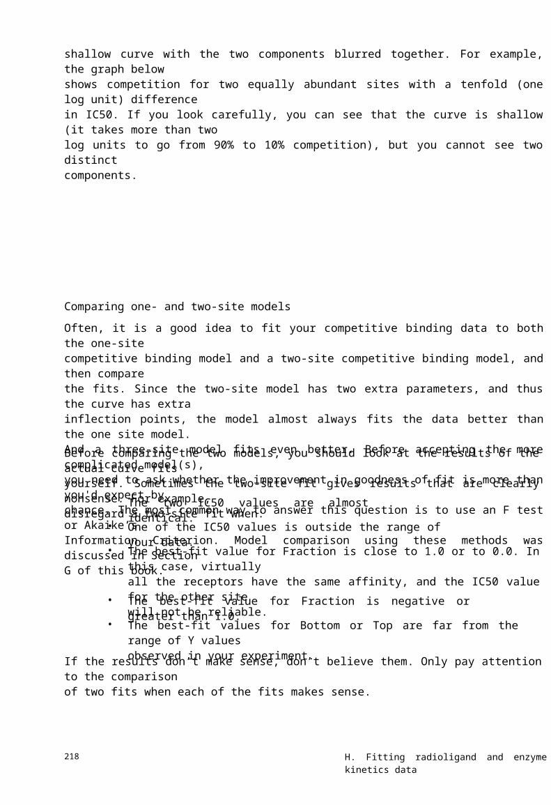
shallow curve with the two components blurred together. For example, the graph belowshows competition for two equally abundant sites with a tenfold (one log unit) differencein IC50. If you look carefully, you can see that the curve is shallow (it takes more than twolog units to go from 90% to 10% competition), but you cannot see two distinctcomponents.

Comparing one- and two-site models

Often, it is a good idea to fit your competitive binding data to both the one-sitecompetitive binding model and a two-site competitive binding model, and then comparethe fits. Since the two-site model has two extra parameters, and thus the curve has extrainflection points, the model almost always fits the data better than the one site model.And a three-site model fits even better. Before accepting the more complicated model(s),you need to ask whether the improvement in goodness of fit is more than you'd expect bychance. The most common way to answer this question is to use an F test or Akaike’sInformation Criterion. Model comparison using these methods was discussed in SectionG of this book.

Before comparing the two models, you should look at the results of the actual curve fitsyourself. Sometimes the two-site fit gives results that are clearly nonsense. For example,disregard a two-site fit when:

•

•

•

The two IC50 values are almost identical.

One of the IC50 values is outside the range of your data.

The best-fit value for Fraction is close to 1.0 or to 0.0. In this case, virtuallyall the receptors have the same affinity, and the IC50 value for the other sitewill not be reliable.

The best-fit value for Fraction is negative or greater than 1.0.

The best-fit values for Bottom or Top are far from the range of Y valuesobserved in your experiment.

•

•

If the results don’t make sense, don’t believe them. Only pay attention to the comparisonof two fits when each of the fits makes sense.


Competitive binding with two receptor types (different Kd for hotligand)The standard equation for competitive binding to two sites assumes that the labeledligand has equal affinity for both sites. It is easy to derive an equation for situations wherethe labeled ligand binds differently to the two sites.

Binding is the sum of specific and nonspecific binding. To create an equation for two sites,you simply need to create an equation with two specific binding components withdifferent values for Bmax, Kd, and Ki: This is shown below as a user-defined equation.

VariableXYHotnM

KD1

KD2

logKI1

logKI2

Bmax1

Unitslog(Molar)cpmnM

nM

nM

log(Molar)

log(Molar)

Units of Y axis,usually cpm

CommentsConcentration of unlabeled drug.Total binding of radioligand.Concentration of labeled ligand added to each tube. Set to aconstant value.Kd of the labeled ligand for the first site. Set to a constantvalue based on other experiments.Kd of the labeled ligand for the second site. Set to aconstant value .Affinity of the unlabeled drug for the first site. Try aninitial value of 1.2 x your mid-range X value.Affinity of the unlabeled drug for the second site. Try aninitial value of 0.8 x your mid-range X value.Try an initial value of 2 x your maximum Y value. (Thisassumes that you've used a concentration of radioligandthat binds to half of the receptors. You may wish to adjustthis.)Try an initial value of 2 x your maximum Y value. (Thisassumes that you've used a concentration of radioligandthat binds to one tenth of the receptors.)Nonspecific binding. Try an initial value of 1 x yourminimum Y value.

Bmax2 Units of Y axis,usually cpm

Units of Y-axis,usually cpm.

NSCPM


Notes:

•

•

This equation does not account for ligand depletion. It assumes that the freeconcentration equals the added concentration.

When using this equation to fit data, you will need to assign constant values toKD1 and KD2, the KD of the hot ligand for the two sites. You will need to obtainthese values from other experiments. Perhaps you can isolate tissue with only oneof the receptor types and measure Kd in that preparation.

Heterologous competitive binding with ligand depletionThe standard sigmoidal equations used to fit competitive binding data assume that asmall fraction of the radioligand binds relative to what is added. This means that the freeconcentration of radioligand is almost equal to the concentration you added, and that thefree concentration is the same in all tubes in the assay.

If a large (say greater than 10%) fraction of the radioligand binds to receptors, then thefree concentration will be less than the added concentration of radioligand. Thediscrepancy between free and added radioligand concentration depends on theconcentration of the unlabeled drug. The standard equation for competitive binding,shown below, needs two corrections to account for ligand depletion.

The nonspecific binding is not the same for all tubes. As you increase the concentration ofcold ligand, less radioligand binds to receptors so the free concentration of radioligandincreases. Since nonspecific binding is assumed to be proportional to the freeconcentration of radioligand, there will be more nonspecific binding in the tubes withhigher concentrations of unlabeled drug.

Y, [Free ligand], and [Added ligand] are expressed in units of cpm. To be consistent,therefore, the Kd also needs to be expressed in cpm units. [Cold ligand] and Ki areexpressed in the same units (molar), so the ratio is unitless.

Combine these equations, and you end up with a complicated quadratic equation whosesolution is shown here:


VariableX

YHot

SpAct

VolKdnMLogKi

Bmax

Unitslog(Molar)

CPMCPM

cpm/fmol

mlnMlog(Molar)

Units of Y axis,usually cpm

CommentsLogarithm of the concentration of unlabelledcompetitor.Bound labeled ligand.Amount of labeled ligand added to each tube.Set to a constant value.Specific radioactivity of labeled ligand. Set toconstant value.Incubation volume. Set to a constant value.

Kd of labeled ligand. Set to a constant value.Try an initial value of 1 x your mid-range XvalueTry an initial value of 10 x your maximal Yvalue (This assumes that you've used aconcentration of radioligand that binds to onetenth of the receptors. You may wish to adjustthis.)Initial value =0.01NS Unitless fraction

You need to set four of the parameters to constant values. Hot is the number of cpm oflabeled ligand added to each tube. SpAct is the specific activity of the radioligand incpm/fmol, Vol is the incubation volume in ml, and KdnM is the Kd of the radioligand innM (determined from other experiments). The nonlinear regression algorithm then fitsthis equation to your data to determine the logKI. It also fits two other variables, whichare of less interest: Bmax, which is the maximum binding of radioligand (if present at asaturating concentration) in cpm, and NS, which is the fraction of the free ligand thatbinds nonspecifically.

Note that this equation accounts for depletion of the hot ligand only, and does not adjustfor depletion of the unlabeled compound. Also note that this equation is not easilyextended to a situation with two binding sites.


38. Homologous competitive binding curves

Introducing homologous competition

The most common way to determine receptor number and affinity is to perform asaturation binding experiment, where you vary the concentration of radioligand. Analternative is to keep the radioligand concentration constant, and compete for bindingwith the same ligand, but not radioactively labeled. Since the hot (radiolabeled) and cold(unlabeled) ligands are chemically identical, this is called a homologous competitivebinding experiment. It is also sometimes called a cold saturation experiment. Anadvantage of performing homologous competition binding experiments for determiningradioligand Kd and Bmax values, rather than the more standard saturation binding method,is that you use less radioligand in the homologous competition experiment and generallyhave lower nonspecific binding than in the saturation assay.

Most analyses of homologous competition data are based on these assumptions:

Assumption

The receptors haveidentical affinity for thelabeled and unlabeledligand.

CommentsThis is a nontrivial assumption. With tritiated ligands, there is noreason to doubt it, since tritium doesn’t greatly alter theconformation of a molecule. However, iodination can changeconformation and alter the binding affinity. Don't assume thatiodinated and noniodinated compounds bind with the sameaffinity. If your radioligand is labeled with radioactive iodine,then you should use a competitor that is the same compoundiodinated with nonradioactive iodine.This means that binding of ligand to one binding site does notchange its affinity at other site(s).

The basic analysis methods assume that only a small fraction ofligand binds. In other words, the method assumes that freeconcentration of hot (and cold) equals the concentration youadded. Since homologous competition curves are best performedwith low concentrations of radioligand, it may be difficult tocomply with this assumption. If a large fraction of radioligandbinds, you can lower the fractional binding by increasing theincubation volume (without increasing the amount of tissue). Alater section in this chapter explains how to analyze data whenthis assumption is not valid.

We assume that a certain fraction of hot ligand bindsnonspecifically, regardless of the concentration of unlabeledligand. This assumption has proven to be true in many systems.

There is nocooperativity.

Ligand is not depleted.

Nonspecific binding isproportional to theconcentration of labeledligand.


Theory of homologous competition binding

Specific binding and Bmax are in the same units, usually cpm, dpm, sites/cell, or fmol/mg.[Hot], [Cold], and Kd are in concentration units. Those units cancel so it doesn’t matter ifyou use molar, nM, or some other unit, so long as you are consistent.

Maximum binding of labeled ligand occurs when the concentration of cold ligand equalszero. This is not the same as Bmax, because the concentration of hot ligand will not saturateall the receptors. In the absence of cold ligand (set [cold]=0), the binding equals

Specific Binding[Cold]=0 =Bmax [Hot]⋅[Hot]+K d

The IC50 in a homologous binding experiment is the concentration of [Cold] that reducesspecific binding of labeled ligand by 50%. So the IC50 is the concentration of cold thatsolves the equation below. The left side of the equation is half the maximum binding withno cold ligand. The right side is binding in the presence of a particular concentration ofcold ligand. We want to solve for [Cold].

0.5 ⋅Bmax [Hot]Bmax [Hot]⋅ ⋅ =[Hot]+K d[Hot]+K d +[Cold]

Solve this equation for [Cold], and you’ll find that you achieve half-maximal binding when[Cold] = [Hot] + Kd. In other words,

IC50 =[Hot]+K d

Why homologous binding data can be ambiguous

Since the IC50 equals [Hot] + Kd, the value of the Kd doesn’t affect the IC50 very muchwhen you use a high concentration of radioligand. This means that you’ll see the sameIC50 with a large range of Kd values. For example, if you use a hot ligand concentration of10 nM, the IC50 will equal 10.1 nM if the Kd is 0.1 nM (dashed curve below), and the IC50will equal 11 nM if the Kd is 1 nM (solid curve below).

38. Homologous competitive binding curves 223

If you used 10 nM of radioligand and your data followed the course of the curves shownabove, the analysis would simply be ambiguous. You wouldn’t know if you have a low Kdwith lots of receptors or a high Kd with few receptors.

If the concentration of hot (radiolabeled) ligand greatly exceeds the Kd, the curve isambiguous. An infinite number of curves, defined by different Kd and Bmax values, arealmost identical. The data simply don’t define the Kd and Bmax . No curve-fitting programcan determine the Kd and Bmax from this type of experiment – the data are consistent withmany Kd and Bmax values.

Using global curve fitting to analyze homologous (one site)competition data

The difficulties associated with fitting homologous binding data discussed above can beminimized by performing the experiment with two, or more, concentrations ofradioligand and using global curve-fitting (parameter sharing) to simultaneously fit theentire family of curves to the homologous binding model.

Tip: We recommend that you perform homologous competition experimentswith at least two radioligand concentrations, and analyze the data using globalcurve fitting.

To fit homologous binding data, we also need to account for the effects of nonspecificbinding. The total measured binding equals specific binding plus nonspecific binding.Nonspecific binding is the same for all tubes since it only depends on the concentration ofhot ligand, which is constant. The equation for specific binding is derived in “Theory ofhomologous competition binding” above. We simply need to add a nonspecific bindingterm to define total binding:

Total Binding = Bmax [Hot]⋅ +NS[Hot]+[Cold]+K d

Here is an equation for homologous competition binding.

ColdNM=10^(x+9)KdNM=10^(logKD+9)Y=(Bmax*HotnM)/(HotnM + ColdNM + KdNM) + NS


This equation assumes that you have entered X values as the logarithm of theconcentrations of the unlabeled ligand in molar, so 1 nM (10-9 molar) is entered as -9. Thefirst line in the equation adds 9 to make it the logarithm of the concentration in nM, andthen takes the antilog to get concentration in nM.

Y is the total binding of the radioligand, expressed in cpm, dpm, fmol/mg, or sites/cell.The Bmax will be expressed in the same units you use for Y.

Since the experiment is performed with the concentrations of unlabeled ligand equallyspaced on a log scale, the confidence intervals will be most accurate when the Kd is fit asthe logKd. The second line converts the log of the Kd in moles/liter to nM.

The equation defines Y (total binding) as a function of X (the logarithm of theconcentration of the unlabeled compound) and four parameters. We are going to useglobal curve fitting to fit both data sets at once, so need to tell the program whichparameters to share.

ParameterBmax

UnitsSame as Y values

CommentsYou want to fit one value of Bmax from both datasets, so set your program to share this parameterbetween data sets.Concentration of labeled ligand in every tube. Setthis to a constant value that you know fromexperimental design. This will have a differentconstant value for each data set. In Prism, makethis a data set constant, so Prism will read itsvalue from the column titles of the data table.You want to fit one value of Kd from both datasets, so set your program to share this parameterbetween data sets.Nonspecific binding depends on how muchradioligand we used. The equation, as writtenabove, adds a constant term NS (in units of Y).Since we expect different amounts of nonspecificbinding at each concentration of hot ligand, wedo not share the value of NS. Instead, we ask thecurve-fitting program to find a different best-fitvalue of NS for each curve.

HotnM nM

LogKd Log(M)

NS Same as Y values

To fit the model, you have to enter or choose initial values for each parameter.

ParameterBmax

UnitsSame as Y values

CommentsTry an initial value of 10 × your maximal Y value (thisassumes that you used a concentration of ligand thatbinds to about one tenth of these receptors).Try an initial value of 1.2 × your mid-range X value.

Try an initial value of 1 × your minimum Y value.

LogKd

NS

Log(moles/liter)

Same as Y values

Shown in the figure below are results of homologous competition binding data using twoconcentrations of radioligand (0.3 and 1 nM). The nonlinear regression was set up so


both the Bmax and the KdnM (Kd in nM concentration units) were shared between the datasets. This means that the program finds a single Bmax and single Kd for both data sets. Aseparate estimate is derived for NS from each data set, however, as each radioligandconcentration will result in a different degree of nonspecific binding. The parameterHotnM was set to a constant value for each data set (0.3 or 1).

GraphPad note: To make a parameter have a different constant value for eachdata set, use Prism’s constraint tab in the nonlinear regression dialog. Set theparameter to be a data set constant, and put the values into the column title ofthe data table. See page 300

The confidence intervals of the global estimates of LogKd and Bmax are reasonable. Bysimultaneously analyzing both data sets, the results are far tighter than they would be ifwe fit each curve separately.

Analyzing homologous (one site) competition data without globalcurve fittingThere are two practical situations where you may not be able to use the global curve-fitting approach outlined above to analyze homologous competition binding data. Thefirst situation is where your nonlinear regression program does not allow you to performglobal curve-fitting with parameter-sharing across data sets. The second situation iswhere you have performed the experiment with only a single concentration of radioligand.

The ambiguity associated with fitting single curves to the homologous binding model hasalready been discussed above. If we take the same example from the previous section, butthis time fit each curve individually instead of globally fitting the model to both data sets,we obtain the following results.


Although the curves fit the data very well, both Bmax and logKd parameters have largestandard errors and accordingly wide 95% confidence intervals. This reflects the difficultyinherent in obtaining reliable parameter estimates from any one homologous competitivebinding curve.

Note: If you have a computer program that can perform global curve fitting,then we recommend you perform any homologous competition experimentusing two radioligand concentrations and globally fit both data sets to thehomologous binding model.

If you cannot use global curve fitting to analyze your data, or you are going to do theexperiment with a single radioligand concentration, then you should follow these steps toensure that you increase your chances of obtaining quality data.

Step 1: Determine the IC50This first step is to check that you used a reasonable concentration of radioligand.

Fit your data to the standard one-site competition equation. If your competitioncurve doesn’t have clearly defined top and bottom plateaus, you should set one or both ofthese to constant values based on control experiments.


Compare the best-fit value of the IC50 to the concentration of hot ligand you used.Homologous competition experiments only lead to useful results when the concentrationof hot ligand is less than half the IC50.

IfIC50 is more than tentimes [Hot]

Then do thisThe concentration of [Hot] is lower than it needs to be. If you havequality data, you can continue with step 2. If you have too few cpmbound or if more than 10% of the added radioactivity binds totissue, rerun the experiment with more radioligandYou’ve designed the experiment appropriately. Continue to step 2to determine the Kd and Bmax with confidence limits.You’ll get better results if you repeat the experiment using less hotligand.

If binding follows the assumptions of the analysis, it is impossiblefor the IC50 to be less than the concentration of hot ligand. SinceKd = IC50 –[Hot], these data would lead to a negative value for Kd ,which is impossible. One possibility is that your system does notfollow the assumptions of the analysis. Perhaps the hot and coldligands do not bind with identical affinities. Another possibility isthat you simply used too high a concentration of hot ligand, so thetrue IC50 is very close to (but greater than) [Hot]. Experimentalscatter may lead to a best-fit IC50 that is too low, leading to theimpossible results. Repeat the experiment using a lot less hotligand.

IC50 is between twoand ten times [Hot]IC50 is greater than[Hot] but not twice ashighIC50 is less than [Hot]

Step 2: Determine Kd and BmaxOnce you’ve determined that the IC50 is quite a bit larger than the concentration of hotligand, fit the homologous competition binding model (see previous section) to determinethe Bmax and Kd. Set HotnM equal to the concentration of labeled ligand in nM, and set itto be a constant value, otherwise the nonlinear regression procedure will not be able toconverge on reasonable estimates for your Bmax and Kd parameters.

If you have performed a series of homologous competition binding experiments usingdifferent radioligand concentrations, but cannot fit your data using global-fitting, you canstill derive useful information from your experiments that can optimize your fit.

From the one-site homologous competition binding model, we have shown previously that

IC50 =[Hot]+K d

By performing a series of homologous competition experiments using differentconcentrations of radioligand, you can plot each IC50 value against the correspondingvalue of [Hot]; a linear regression of these data should yield an estimate of the Kd value.Unfortunately, you cannot determine Bmax from this approach.


Homologous competitive binding with ligand depletion

If a large fraction of the radioligand is bound to the receptors, homologous binding will beaffected. Although you add the same amount of labeled ligand to each tube, the freeconcentration will not be the same. High concentrations of unlabeled drug compete forthe binding of the labeled ligand, and thus increase the free concentration of the labeledligand.

Nonspecific binding is also affected by ligand depletion. Since nonspecific binding isproportional to the free concentration of labeled ligand, the amount of nonspecificbinding will not be the same in all tubes. The tubes with the highest concentration ofunlabeled drug have the highest concentration of free radioligand, so they will have themost nonspecific binding.

Because the free concentration varies among tubes, as does the nonspecific binding, thereis no simple relationship between IC50 and Kd. The IC50 is nearly meaningless in ahomologous binding curve with ligand depletion.

The equations for homologous binding with ligand depletion are quite a bit morecomplicated than for homologous binding without depletion. The math that follows isadapted from S. Swillens (Molecular Pharmacology, 47: 1197-1203, 1995).

Start with the equation for total binding in homologous competition as a function of thefree concentration of radioligand.

This equation defines total binding as specific binding plus nonspecific binding.Nonspecific binding equals a constant fraction of free radioligand, and we define thisfraction to be NS. To keep units consistent, the radioligand concentration is expressed innM in the left half of the equation (to be consistent with Kd and the concentration of coldligand) and is expressed in cpm on the right half of the equation (to be consistent with Y).

The problem with this equation is that you don't know the concentrations of freeradioligand or free cold ligand. What you know are the concentrations of labeled andunlabeled ligand you added. Since a high fraction of ligand binds to the receptors, youcannot assume that the concentration of free ligand equals the concentration of addedligand.

Defining the free concentration of hot ligand is easy. You added the same number of cpmof hot ligand to each tube, which we'll call HotCPM. The concentration of free radioligandequals the concentration added minus the total concentration bound, or HotCPM-Y (bothHotCPM and Y are expressed in cpm).

Defining the free concentration of cold ligand is harder, so it is done indirectly. Thefraction of hot radioligand that is free equals (HotCPM - Y)/HotCPM. This fraction will bedifferent in different tubes. Since the hot and cold ligands are chemically identical, thefraction of cold ligand that is free in each tube is identical to the fraction of hot ligand thatis free. Define X to be the logarithm of the total concentration of cold ligand, the variableyou vary in a homologous competitive binding experiment. Therefore, the total


When fitting data to this equation, you need to set three parameters to constant values.HotCPM is the number of cpm of hot ligand added to each tube. Vol is the incubationvolume in ml. SpAct is the specific radioactivity in cpm/fmol. The nonlinear regressionalgorithm then fits Bmax in the units of the Y axis (usually cpm, which you can convert tomore useful units) and logKd as log molar.

As with homologous binding data without ligand depletion, we recommend that youperform the experiment using more than one radioligand concentration and fit the datausing global-fitting to share a single Bmax value and single Kd value across all data sets.


VariableXYHotCPM

SpAct

VollogKdBmax

Unitslog(Molar)cpmcpm

cpm/fmol

mlLog(Molar)

Comments

Amount of labeled ligand added to each tube. Set to aconstant value.Specific radioactivity of labeled ligand. Set to aconstant value.Incubation volume. Set to a constant value.Initial value = 1 x the mid-range X value

Units of Y axis, usually Initial value = 10 x your maximal Y value (Thiscpmassumes that you've used a concentration of radioligand that binds to one tenth of the receptors. You may wish to adjust this.)Unitless fraction This is the fraction of free ligand that binds

nonspecifically. Initial value =0.01NS

Fitting homologous competition data (two sites)

With some systems it is possible to determine Kd and Bmax values for two independentsites using homologous competition data. With most systems, however, you won’t getreliable results.

You can only determine Bmax and Kd from homologous binding data if you use aconcentration of hot ligand that is much lower than the Kd value. If your system has twobinding sites, you must choose a concentration much lower than the Kd of the high affinitysite. Using such a low concentration of radioligand, you’ll bind only a small fraction oflow-affinity sites. You will only be able to detect the presence of the second, low-affinity,site if they are far more abundant than the high-affinity sites.

For example, imagine that the low affinity site (Kd=10 nM) is ten times as abundant as thehigh-affinity site (Kd=0.1 nM). You need to use a concentration of hot ligand less than 0.1nM, say 0.05 nM. At this concentration you bind to 33.33% of the high-affinity sites, butonly to 0.0049% of the low affinity sites. Even though the low-affinity sites are ten timesas abundant, you won’t find them in your assay (low-affinity binding will be only 0.15% ofthe binding).

To attempt to determine the two Kd and Bmax values from a homologous competitioncurve, fit the data to the equation below. Assuming no cooperativity and no liganddepletion, the binding to each site is independent and depends on the Bmax and Kd valuesof each site. The binding that you measure, Y, is the sum of the binding to the two receptorsites plus nonspecific binding.

This is a difficult equation to fit, and you will almost certainly have to try many sets ofinitial values to converge on a reasonable solution. It is especially important to adjust theinitial values of the two Bmax values.


VariableXY

Bmax1

Unitslog(molar)cpm or fmol/mgor sites/cell.Same as Yvalues.

Same as Yvalues.

log(molar)log(molar)Same as Yvalues.nM

CommentsConcentration of the unlabeled compound.Total binding of the labeled compound.

Initial value =1 x your maximum Y value (this assumesthat you used a concentration of ligand that binds toalmost all of the high affinity class of receptors).Initial value = 20 x your maximum Y value (thisassumes that you used a concentration of ligand thatbinds to five percent of the second class of receptors).Initial value = 1.2 x your mid-range X value.Initial value = 0.8 x your mid-range X value.Initial value = = 1. x your minimum Y value.

Concentration of labeled ligand in every tube. Set this toa constant value that you know from your experimentaldesign.

Bmax2

LogKd1LogKd2

NS

HotnM

Consider this approach for analyzing homologous competitive binding data to determinethe characteristics of two sites. First use a very low concentration of radioligand and fit toa single site. This will determine the Bmax and Kd of the high affinity site. Then repeat theexperiment with a higher concentration of radioligand. Fit these data to the two-siteequation, but set Kd and Bmax for the high affinity site to constant values determinedfrom the first experiment. Alternatively, and if your nonlinear regression program allowsit, you can perform a global fit of both equations simultaneously to both data sets by usingparameter-sharing, similar to the detailed method outlined above for homologouscompetition binding to one binding site.

Advantages and disadvantages of homologous binding experimentsDetermining receptor number with homologous binding has one clear advantage: Youneed far less radioligand than you would need if you performed a saturation bindingexperiment. This reason can be compelling for ligands that are particularly expensive ordifficult to synthesize.

The disadvantage of determining receptor number and affinity from a homologouscompetitive binding experiment is that it can be hard to pick an appropriate concentrationof radioligand. If you use too little radioligand, you’ll observe little binding and will obtainpoor quality data. If you use too much radioligand, the curve will be ambiguous and youwon’t be able to determine Bmax and Kd. The use of a minimum of two different radioligandconcentrations in a homologous binding assay, in conjunction with the global curve-fittingapproach outlined above, provides the best compromise between saturation bindingassays and standard (one-curve) homologous competition binding assays.

Using homologous binding to determine the Kd and Bmax of two binding sites with isdifficult, even with multiple radioligand concentrations. You are probably better off usinga saturation binding experiment.


39. Analyzing kinetic binding data

Dissociation ("off rate") experiments

A dissociation binding experiment measures the “off rate” for radioligand dissociatingfrom the receptor. Initially ligand and receptor are allowed to bind, perhaps toequilibrium. At that point, you need to block further binding of radioligand to receptor soyou can measure the rate of dissociation. There are several ways to do this:

•

•

•

If the tissue is attached to a surface, you can remove the buffer containingradioligand and replace with fresh buffer without radioligand.

Spin the suspension and resuspend in fresh buffer.

Add a very high concentration of an unlabeled ligand. If this concentration ishigh enough, it will instantly bind to nearly all the unoccupied receptors andthus block binding of the radioligand.

Dilute the incubation by a large factor, at least 100 fold dilution. This willreduce the concentration of radioligand by that factor. At such a lowconcentration, new binding of radioligand will be negligible. This method isonly practical when you use a fairly low concentration of radioligand so itsconcentration after dilution is far below its Kd for binding.

•

You then measure binding at various times after that to determine how rapidly theradioligand falls off the receptors.

39. Analyzing kinetic binding data 233

VariableX

Y

Span

MeaningTime

Total binding

Difference betweenbinding at time zero andplateau.Binding that doesn'tdissociate.Dissociation rateconstant often called koff.

CommentUsually expressed in units of seconds orminutes.Usually expressed in units of cpm, dpm,fmol/mg, or sites/cell.Specific binding (same units as Y).

Plateau

K

Nonspecific binding (same units as Y).

Expressed in units of inverse time (inverse ofunits of X-axis).

Analyzing dissociation dataTo analyze dissociation binding data:

1.

2.

3.

Enter the data with X equal to time after you initiated dissociation and Y equal tobinding (usually total binding).

Perform nonlinear regression using an exponential decay equation.

If you entered specific (rather than total) binding as your dependent variable,make the parameter, Plateau, a constant equal to zero. If you have entered totalbinding, leave the parameter Plateau as to be fitted.

Look at the nonlinear regression results. The variable K is the dissociationconstant (often referred to in texts as koff or k-1) expressed in units of inverse time.If you entered the X values as minutes, koff is in units of min-1. The results alsoshow the half-life in units of time (minutes in this example).

You can use the koff value to determine the half-life (t1/2) of dissociation. Use thefollowing relationship: t1/2 = 0.693/koff.

4.

5.

Association binding experiments

Association binding experiments are used to determine the association rate constant. Youadd radioligand and measure specific binding at various times thereafter.

Binding follows the law of mass action:

Kon→Receptor + LigandReceptor gLigand ← Koff

At any given time, the rate at which receptor-ligand complexes form is proportional to theradioligand concentration and the number of receptors still unoccupied. The rate ofdissociation is proportional to the concentration of receptor-ligand complexes.


Binding increases over time until it plateaus when specific binding equals a value we callYmax. This is not the same as Bmax. Ymax is the amount of specific binding at equilibrium fora certain concentration of ligand used in an association experiment. Bmax is the maximumamount of binding extrapolated to a very high concentration of ligand. These principles letus define the model mathematically.

The rate at which binding increases is determined by three factors (for a constant set ofexperimental conditions such as pH and temperature):

•

•

•

The association rate constant, kon or k+1. This is what you are trying to determine.

The concentration of radioligand. If you use more radioligand, the systemequilibrates faster.

The dissociation rate constant, koff or k-1. Some people are surprised to see that theobserved rate of association depends in part on the dissociation rate constant.


During the incubation, radioligand both binds to and dissociates from receptors.The system reaches equilibrium when the two rates are equal. The observed rateof association measures how long it takes to reach equilibrium. If the radioliganddissociates quickly from the receptor, equilibrium will be reached faster (but withless binding).

Analyzing "on rate" experimentsTo analyze association (on-rate) data:

1. Enter the data with X equal to time and Y equal to specific binding. (If you entertotal binding, you'll need to use a more complicated equation that accounts for thekinetics of nonspecific binding.)

Fit the specific binding data to an exponential association equation. The simplestcase, one-phase exponential association, is shown here:

2.

Y=Ymax (1-e-k X )⋅ ⋅

3. The variable k in the exponential association equation is the observed rateconstant, kob, expressed in units of inverse time. If you entered X values inminutes, then k is expressed in min-1. This is not the same as the association

obrate constant, kon.

4. This equation assumes that a small fraction of the radioligand binds to receptors,so the concentration of free radioligand equals the amount you added and doesnot change over time.

To calculate the association rate constant (kon or k1), usually expressed in units ofMolar-1 min-1, use this equation:

5.

Variablekon

kob

koff

Units

min-1

min-1

Comment

The value of K determined by fitting an exponential associationequation to your data.The dissociation rate constant. See the previous section.

Set by the experimenter. Assumed to be constant during theexperiment (only a small fraction binds).

Molar-1 min-1 Association rate constant; what you want to know.

[radioligand] Molar

Fitting a family of association kinetic curves

If you perform your association experiment at a single concentration of radioligand, itcannot be used to determine kon unless you are able to fix the value of koff from anotherexperiment.


If you perform multiple association kinetic experiments, each with a different radioligandconcentration, you can globally fit the data to the association kinetic model to derive asingle best-fit estimate for kon and one for koff. You don’t need to also perform adissociation (off rate) experiment.

Shown below is an example of an association kinetic experiment conducted using twoconcentrations of radioligand. All other conditions (temperature, pH, etc.) were the samefor both runs, of course. Times were entered into the X column, specific binding for oneconcentration of radioligand were entered into the first (A) Y column, and binding for theother concentration were entered into column B.

The first line defines the intermediate variable Radioligand for data set A. Theconcentration is 1nM, and it is expressed in scientific notation as 1 x 10-9 molar. Thesecond line defines the variable Radioligand for data set B. The third line defines theobserved rate constant as a function of radioligand concentration and the two rateconstants. The final line computes Y (specific binding) for any value of X (time).

You could also enter the model in a simpler form into Prism.

This model does not define the parameter radioligand. Instead, enter the concentrationsas the column titles of columns A and B, and define the parameter Radioligand to be adata set constant within Prism. See page 300.


Globally fitting an association curve together with a dissociationcurve

Another way to determine both association and dissociation rate constants from oneexperiment is to run an experiment that first measures ligand association, and thenmeasures ligand dissociation.

For example in the experiment below, radioligand was added at time zero, and totalbinding was measured every five minutes for one hour. At time = 60, a very highconcentration of unlabeled drug was added to the tubes. This entirely blocked newbinding of radioligand to the receptors. Every five minutes, total binding was measured asa way to assess the rate of ligand dissociation.

Variable Explanation Units Kind of variableRadioligand The concentration of

radioactively labeled ligand.Molar Constant. We set its

value within theequation. An alternativewould have been to set itto a constant value in thenonlinear regressiondialog.


Variable Explanation Units Kind of variableKob The apparent “on rate” calculated

from the concentration ofradioligand with the associationand dissociation rate constants.

Association rate constant.

Dissociation rate constant.

The time when dissociation wasinitiated.

min-1 Intermediate variable,defined within theequation forconvenience.

Parameter to fit.

Parameter to fit.

Constant. We set itsvalue within theequation. An alternativewould have been to set itto a constant value in thenonlinear regressiondialog.

Intermediate variable,defined within theequation forconvenience.


Parameter to fit.

Kon

Koff

Time0

M-1 min-1

min-1

min

Kd The dissociation constant for thereceptor-ligand binding, inMolar.

The amount of binding (in cpm, tomatch the Y values) at equilibrium.Calculated from the concentrationof radioligand we used and its Kd.This is an intermediate variable,defined within the equation.

min-1

Eq cpm

Bmax The maximum amount ofbinding sites. This is not themaximum bound at theconcentration of ligand we chose,but the maximum number ofsites that can binding ligand.

The predicted binding atX=Time0. The dissociation partof the experiment begins withthis amount of binding.

The predicted Y values for theassociation part of theexperiment (up to X=60). Inunits

The predicted Y values for thedissociation part of theexperiment (after time X=60).

Nonspecific binding. Assumed tobe constant over time. In units ofcpm (to match Y).

cpm

YatTime0 cpm Intermediate variable,defined within theequation forconvenience.



We set this to a constantvalue based on goodcontrol measurements.

239

Associationcpm

Dissociation cpm

NS cpm


Variable Explanation Units Kind of variableAn alternative wouldhave been to make this aparameter to fit.

X

Y

Time

Total binding

minutes

cpm

Independent variable

Dependent variable

Association computes the association of a ligand over time. Dissociation computes thedissociation of a ligand after time0. The final line uses an IF statement (Prism syntax) todefine Y equal to Association before time0 and equal to dissociation thereafter, and thenadds the nonspecific binding (NS).

The model has three parameters to fit: the association rate constant, the dissociation rateconstant, and the maximum number of binding sites.

Note: This is not strictly a global model, as it fits one data set and not several.But it fits one model (exponential association) to part of the data set andanother model (exponential decay) to another portion of the data set. This iseffectively a form of global fitting.

Analysis checklist for kinetic binding experiments

QuestionDid you go out to a longenough time point?Is the value of konreasonable?

CommentDissociation and association data should plateau, so the data obtainedat the last few time points should be indistinguishable.

The association rate constant, kon, depends largely on diffusion so issimilar for many ligands. Expect a result of about 107 - 108 M-1 min-1


Is the value of koffreasonable?

If the koff is greater than 1 min-1, the ligand has a low affinity for thereceptor, dissociation will occur while you are separating bound andfree ligands, and you'll have a hard time obtaining quality data. If koffis less than 0.001 min-1 , you'll have a difficult time obtainingequilibrium as the half-time of dissociation will be greater than 10hours! Even if you wait that long, other reactions may occur that ruinthe experiment.

Examine the SE and the confidence intervals to see how muchconfidence you have in the rate constants.

The standard analyses of association experiments assume that theconcentration of free radioligand is constant during the experiment.This will be approximately true only if a tiny fraction of the addedradioligand binds to the receptors. Compare the maximum totalbinding in cpm to the amount of added radioligand in cpm. If thatratio exceeds 10% or so, you should revise your experimental protocol.

Are the standard errorstoo large?Does only a tiny fractionof radioligand bind tothe receptors?

Using kinetic data to test the law of mass action

Standard binding experiments are usually fit to equations derived from the law of massaction. Kinetic experiments provide a more sensitive test than equilibrium experiments todetermine whether the law of mass action actually applies for your system. To test the lawof mass action, ask these questions:

Does the Kd calculated from kinetic data match the Kd calculated fromsaturation binding?

The units are consistent: koff is in units of min-1; kon is in units of M-1min-1, so Kd is in unitsof M.

If binding follows the law of mass action, the Kd calculated this way should be the same asthe Kd calculated from a saturation binding curve.

Does kob increase linearly with the concentration of radioligand?

Therefore, if you perform association rate experiments at various concentrations ofradioligand, the results should look like the figure below. As you increase theconcentration of radioligand, the observed rate constant increases linearly. If the bindingis more complex than a simple mass action model (such as a binding step followed by aconformational change) the plot of kob vs. [radioligand] may plateau at higher radioligandconcentrations. Also, you should extrapolate the plot back to zero radioligand todetermine the intercept, which equals koff. If the law of mass action applies to your system,the koff determined this way should correspond to the koff determined from a dissociationexperiment. Finally, this kind of experiment provides a more rigorous determination ofkon than that obtained with a single concentration of radioligand.


Is specific binding 100% reversible, and is the dissociated ligandchemically intact?Nonspecific binding at "time zero" should equal total binding at the end (plateau) of thedissociation. In other words, all of the specific binding should dissociate if you wait longenough. Use chromatography to analyze the radioligand that dissociates to prove that ithas not been altered.

Is the dissociation rate consistent with different experimentalconditions?Determine the dissociation constant after binding various concentrations of radioligandfor various lengths of time. If your ligand binds to a single site and obeys the law of massaction, you'll obtain the same dissociation rate constant in all experiments.

Is there cooperativity?If the law of mass action applies, binding of a ligand to one binding site does not alter theaffinity of another binding site. This also means that dissociation of a ligand from one siteshould not change the dissociation of ligand from other sites. To test this assumption,compare the dissociation rate after initiating dissociation by infinite dilution with thedissociation rate when initiated by addition of a large concentration of unlabeled drug. Ifthe radioligand is bound to multiple noninteracting binding sites, the dissociation will beidentical in both experimental protocols as shown in the left figure. Note that the Y axis isshown using a log scale. If there were a single binding site, you'd expect the dissociationdata to appear linear on this graph. With two binding sites, the graph is curved even on alog axis.


The right figure shows ideal dissociation data when radioligand is bound to interactingbinding sites with negative cooperativity. The data are different depending on howdissociation was initiated. If dissociation is initiated by infinite dilution, the dissociationrate will change over time. The dissociation of some radioligand will leave the remainingligand bound more tightly. When dissociation is initiated by addition of cold drug, all thereceptors are always occupied by ligand (some hot, some cold) and dissociation occurs atits maximal unchanging rate.

Kinetics of competitive binding

The standard methods of analyzing competitive binding experiments assume that theincubation has reached equilibrium. These experiments are usually used to learn thedissociation constant of the receptors for the unlabeled compound, the Ki. The law of massaction tells us that the Ki is the ratio of the off-rate to the on-rate of the unlabeledcompound. You can determine these values in a kinetics experiment as follows. Addlabeled and unlabeled ligand together and measure the binding of the labeled ligand overtime. This method was described by Motulsky and Mahan in Mol. Pharmacol. 25:1-9,1984.

VariableXYk1

k2

k3

k4

L

Bmax

UnitsMinutescpmM-1 min-1

min-1

M-1 min-1

min-1

nM

CommentsTime.Specific binding.Association rate constant of radioligand. Set to a constant valueknown from other experiments.Dissociation rate constant of radioligand. Set to a constant valueknown from other experiments.

Association rate constant of unlabeled ligand. Variable to be fit. Try108 as an initial value.

Dissociation rate constant of unlabeled ligand. Variable to be fit.Try 0.01 as an initial value.Concentration of radioligand. Set to a constant value you knowfrom experimental design.

Units of YTotal number of receptors. Either leave as a variable or set to aaxis. Usually constant you know from other experiments. If a variable, set thecpm.initial value to 100 x your maximal Y value (assumes that it binds to 1% of receptors.nM Constant set experimentally. Concentration of unlabeled ligand.I

Notes:


• This equation does not account for ligand depletion. It assumes that only asmall fraction of radioligand binds to receptors, so that the freeconcentration of radioligand is very close to the added concentration.

This method will only give reliable results if you have plenty of data points atearly time points.

•


40. Analyzing enzyme kinetic data

Introduction to enzyme kinetics

Living systems depend on chemical reactions which, on their own, would occur atextremely slow rates. Enzymes are catalysts that reduce the needed activation energy sothese reactions proceed at rates that are useful to the cell.

Product accumulation is often linear with timeIn most cases, an enzyme converts one chemical (the substrate) into another (theproduct). A graph of product concentration vs. time follows three phases.

1. At very early time points, the rate of product accumulation increases over time.Special techniques are needed to study the early kinetics of enzyme action, sincethis transient phase usually lasts less than a second (the figure greatly exaggeratesthe first phase).

For an extended period of time, the product concentration increases linearly withtime.

At later times, the substrate is depleted, so the curve starts to level off. Eventuallythe concentration of product reaches a plateau.

2.

3.

It is difficult to fit a curve to a graph of product as a function of time, even if you use asimplified model that ignores the transient phase and assumes that the reaction isirreversible. The model simply cannot be reduced to an equation that expresses productconcentration as a function of time. To fit these kind of data (called an enzyme progresscurve) you need to use a program that can fit data to a model defined by differentialequations or by an implicit equation. For more details, see RG Duggleby, "Analysis ofEnzyme Reaction Progress Curves by Nonlinear Regression", Methods in Enzymology,249: 61-60, 1995.

Rather than fit the enzyme progress curve, most analyses of enzyme kinetics fit the initialvelocity of the enzyme reaction as a function of substrate concentration. The velocity ofthe enzyme reaction is the slope of the linear phase of product accumulation, expressed asamount of product formed per time. If the initial transient phase is very short, you cansimply measure product formed at a single time, and define the velocity to be theconcentration divided by the time interval.

40. Analyzing enzyme kinetic data 245

The terminology describing these phases can be confusing. The second phase is oftencalled the "initial rate", ignoring the short transient phase that precedes it. It is also called"steady state", because the concentration of enzyme-substrate complex doesn't change.However, the concentration of product accumulates, so the system is not truly at steadystate until, much later, the concentration of product truly doesn't change over time. Thischapter considers data collected only in the second phase.

Enzyme velocity as a function of substrate concentrationIf you measure enzyme velocity at many different concentrations of substrate, the graphgenerally looks like this:

Vmax is the limiting velocity as substrate concentrations get very large. Vmax (and V) areexpressed in units of product formed per time. If you know the molar concentration ofenzyme, you can divide the observed velocity by the concentration of enzyme sites in theassay, and express Vmax in units of moles of product formed per second per mole ofenzyme sites. This is the turnover number, also called kcat. It is the number of molecules ofsubstrate converted to product by one enzyme site per second. In defining enzymeconcentration, distinguish the concentration of enzyme molecules from the concentrationof enzyme sites (if the enzyme is a dimer with two active sites, the molar concentration ofsites is twice the molar concentration of enzyme).

Km is expressed in units of concentration, usually in molar units. Km is the concentrationof substrate that leads to half-maximal velocity. To prove this, set [S] equal to Km in theequation above. Cancel terms and you'll see that V=Vmax/2.

The meaning of KmTo understand the meaning of Km, you need to have a model of enzyme action. Thesimplest model is the classic model of Michaelis and Menten, which has proven usefulwith many kinds of enzymes.


The substrate (S) binds reversibly to the enzyme (E) in the first reaction. In most cases,you can't measure this step. What you measure is production of product (P), created bythe second reaction.

From the model, we want to derive an equation that describes the rate of enzyme activity(amount of product formed per time interval) as a function of substrate concentration.

The rate of product formation equals the rate at which ES turns into E+P, which equals k2times [ES]. This equation isn't helpful, because we don't know ES. We need to solve for ESin terms of the other quantities. This calculation can be greatly simplified by making tworeasonable assumptions. First, we assume that the concentration of ES is steady duringthe time intervals used for enzyme kinetic work. That means that the rate of ES formationequals the rate of ES dissociation (either back to E+S or forward to E+P). Second, weassume that the reverse reaction (formation of ES from E+P) is negligible, because we areworking at early time points where the concentration of product is very low.

Note that Km is not a binding constant that measures the strength of binding between theenzyme and substrate. Its value includes the affinity of substrate for enzyme, but also therate at which the substrate bound to the enzyme is converted to product. Only if k2 ismuch smaller than k-1 will Km equal a binding affinity.

The Michaelis-Menten model is too simple for many purposes. The Briggs-Haldane modelhas proven more useful:


Under the Briggs-Haldane model, the graph of enzyme velocity vs. substrate looks thesame as under the Michaelis-Menten model, but Km is defined as a combination of all fiveof the rate constants in the model.

Assumptions of enzyme kinetic analysesStandard analyses of enzyme kinetics (the only kind discussed here) assume:

•

•

The production of product is linear with time during the time interval used.

The concentration of substrate vastly exceeds the concentration of enzyme. Thismeans that the free concentration of substrate is very close to the concentrationyou added, and that substrate concentration is constant throughout the assay.

A single enzyme forms the product.

There is negligible spontaneous creation of product without enzyme

No cooperativity. Binding of substrate to one enzyme binding site doesn'tinfluence the affinity or activity of an adjacent site.

Neither substrate nor product acts as an allosteric modulator to alter the enzymevelocity.

•

•

•

•

How to determine Vmax and Km

To determine Vmax and Km:

1.

2.

Enter substrate concentrations into the X column and velocity into the Y column(entering replicates if you have them).

Enter this equation as a new equation into your program, and fit it to your datausing nonlinear regression.

Y = (Vmax * X)/(Km + X)

VariableX

Y

CommentSubstrate concentration. Usually expressed in µM or mM.

Enzyme velocity in units of concentration of product per time. It issometimes normalized to enzyme concentration, so concentration ofproduct per time per concentration of enzyme.The maximum enzyme velocity. A reasonable rule for choosing an initialvalue might be that Vmax equals 1.0 times your maximal Y value. Vmax isexpressed in the same units as the Y values.The Michaelis-Menten constant. A reasonable rule for choosing an initialvalue might be 0.2 x your maximal X value.

Vmax

Km

Checklist for enzyme kineticsWhen evaluating results of enzyme kinetics, ask yourself these questions:


QuestionWas only a small fraction ofthe substrate converted toproduct?

CommentThe analysis assumes that the free concentration of substrateis almost identical to the concentration you added during thetime course of the assay. You can test this by comparing thelowest concentration of substrate used in the assay with theconcentration of product created at that concentration.Check the concentration of product at several times to testthis assumption.Calculate the ratio of the highest substrate concentration youused divided by the best-fit value of Km (both in the sameconcentration units). Ideally, the highest concentrationshould be at least 10 times the Km.Divide the SE of the Vmax by the Vmax, and divide the SE of theKm by the Km. If either ratio is much larger than about 20%,look further to try to find out why.The analysis assumes that all product formation is due to theenzyme. If some product is produced spontaneously, you'llneed to do a fancier analysis to account for this.Measure product formation at several time points straddlingthe time used for the assay. The graph of productconcentration vs. time should be linear.The standard analysis assumes no cooperativity. This meansthat binding of substrate to one binding site does not alterbinding of substrate to another binding pocket. Since manyenzymes are multimeric, this assumption is often not true. Ifthe graph of V vs. [S] looks sigmoidal, see "Allostericenzymes" on page 251.

Is the production ofproduct linear with time?Did you use high enoughconcentrations ofsubstrate?

Are the standard errors toolarge? Are the confidenceintervals too wide?Is product produced in theabsence of enzyme?

Did you pick a time point atwhich enzyme velocity isconstant?

Is there any evidence ofcooperativity?

Comparison of enzyme kinetics with radioligand binding

The Michaelis-Menten equation for enzyme activity has a mathematical form similar tothe equation describing equilibrium binding.

Enzyme Velocity=V=

Specific Binding=B=

Vmax [S][S]+K m

Bmax [L][L]+K d

However, the parameters mean different things. Note these differences between bindingexperiments and enzyme kinetics.

• It usually takes many minutes or hours for a receptor incubation to equilibrate. Itis common (and informative) to measure the kinetics prior to equilibrium.Enzyme assays reach steady state (defined as constant rate of productaccumulation) typically in a few seconds. It is uncommon to measure the kineticsof the transient phase before that, although you can learn a lot by studying thosetransient kinetics (see an advanced text of enzyme kinetics for details).

The equation used to analyze binding data is valid at equilibrium - when the rateof receptor-ligand complex formation equals the rate of dissociation. The equation

249

•

40. Analyzing enzyme kinetic data

used to analyze enzyme kinetic data is valid when the rate of product formation isconstant, so product accumulates at a constant rate. But the overall system is notat equilibrium in enzyme reactions, as the concentration of product is continuallyincreasing.

• Kd is a dissociation constant that measures the strength of binding betweenreceptor and ligand. Km is not a binding constant. Its value includes the affinity ofsubstrate for enzyme, but also the kinetics by which the substrate bound to theenzyme is converted to product

Bmax is measured as the number of binding sites normalized to amount of tissue,often fmol per milligram, or sites/cell. Vmax is measured as moles of productproduced per minute.

•

Displaying enzyme kinetic data on a Lineweaver- Burk plot

The best way to analyze enzyme kinetic data is to fit the data directly to the Michaelis-Menten equation using nonlinear regression. Before nonlinear regression was available,investigators had to transform curved data into straight lines, so they could analyze withlinear regression.

Use the Lineweaver-Burk plot only to display your data. Don't use the slope and interceptof a linear regression line to determine values for Vmax and Km. If you do this, you won't getthe most accurate values for Vmax and Km. The problem is that the transformations(reciprocals) distort the experimental error, so the double-reciprocal plot does not obeythe assumptions of linear regression. Use nonlinear regression to obtain the most accuratevalues of Km and Vmax (see page 19).

Tip: You should analyze enzyme kinetic data with nonlinear regression, notwith Lineweaver-Burk plots. Use Lineweaver-Burk plots to display data, not toanalyze data.


Allosteric enzymesOne of the assumptions of Michaelis-Menten kinetics is that there is no cooperativity. Ifthe enzyme is multimeric, then binding of a substrate to one site should have no effect onthe activity of neighboring sites. This assumption is often not true.

If binding of substrate to one site increases the activity of neighboring sites, the termpositive cooperativity is used. Activity is related to substrate concentration by thisequation:

Vmax [S]hVelocity=V= hh[S] +K 0.5

When the variable h equals 1.0, this equation is the same as the Michaelis-Mentenequation. With positive cooperativity, h will have a value greater than 1.0. If there are twointeracting binding sites, h will equal between one and two, depending on the strength ofthe cooperativity. If there are three interacting binding sites, h will equal between 1 and 3.Note that the denominator has the new parameter, K0.5, instead of Km.

To fit data to the equation for enzyme activity with positive cooperativity, use the equationbelow. For initial values, try these rules: Vmax=1 x your maximal Y value, K=0.5 x yourmaximal X value, and h=1.0

The parameter h does not always equal the number of interacting binding sites (althoughh cannot exceed the number of interacting sites). Think of h as an empirical measure ofthe steepness of the curve and the presence of cooperativity.

Enzyme kinetics in the presence of an inhibitor

Competitive inhibitorsIf an inhibitor binds reversibly to the same site as the substrate, the inhibition will becompetitive. Competitive inhibitors are common in nature.


One way to measure the effect of an inhibitor is to measure enzyme velocity at a variety ofsubstrate concentrations in the presence and absence of an inhibitor. As the graph belowshows, the inhibitor substantially reduces enzyme velocity at low concentrations ofsubstrate, but doesn't alter velocity very much at very high concentrations of substrate.

As the graph above shows, the inhibitor does not alter Vmax, but it does increase theobserved Km (concentration of substrate that produces half-maximal velocity; some textscall this “apparent Km”). The observed Km is given by the following equation, where Ki isthe dissociation constant for inhibitor binding (in the same concentration units as[Inhibitor]):

Using global fitting to fit KiThe best way to find the best-fit value of Ki is to fit all your data at once using globalnonlinear regression. Fit to this model.

VariableX

Y

CommentSubstrate concentration. Usually expressed in µM or mM.

Enzyme velocity in units of concentration of product per time. It issometimes normalized to enzyme concentration, so concentration ofproduct per time per concentration of enzyme.The maximum enzyme velocity, in the absence of inhibitor. A reasonablerule for choosing an initial value might be that Vmax equals 1.0 times yourmaximal Y value. Vmax is expressed in the same units as the Y values. Sharethis parameter to get one best-fit value for the entire experiment.The Michaelis-Menten constant, in the same units as X. A reasonable rulefor choosing an initial value might be 0.2 x your maximal X value. Share thisparameter to get one best-fit value for the entire experiment.The inhibition constant, in the same units as your X values and Km. Share.The concentration of inhibitor, in the same units as Ki. For each data set,this is a constant that you enter.

H. Fitting radioligand and enzyme kinetics data

Vmax

Km

KiI

252

Fit the family of curves, setting up the global curve fitting to share the parameters Vmax,Km, and Ki. This means you’ll get one best-fit value for each of these parameters from theentire set of experiments. Set I to be a constant whose value varies with each data set. Thefirst data set is a control, where I equals 0.

GraphPad note: In Prism, enter each inhibitor concentration as the column titlefor the appropriate data set. In the nonlinear regression dialog (constraintstab), define I (inhibitor concentration) to be a data set constant. This meansthat Prism will get its value from the heading of each column.

GraphPad note: The companion step-by-step example book has detailedinstructions for fitting a family of enzyme inhibition curves to determine the Ki.You’ll also find this example at www.graphpad.com.

Finding Ki without global fittingIf you don’t have a program that can fit data with global nonlinear regression, you can usea less accurate method.

If you have determined the Km in the presence and absence of a single concentration ofinhibitor, you can rearrange that equation to determine the Ki.

You'll get a more reliable determination of Ki if you determine the observed Km at a varietyof concentrations of inhibitor. Fit each curve to determine the observed Km. Enter theresults onto a new table, where X is the concentration of inhibitor and Y is the observedKm. If the inhibitor is competitive, the graph will be linear. Use linear regression todetermine the X and Y intercepts. The Y-axis intercept equals the Km and the X-axisintercept equals the negative Ki.


Another approach is to measure enzyme velocity at a single concentration of substratewith varying concentrations of a competitive inhibitor. The results will look like this.

The concentration of competitor that reduces enzyme velocity by half is called the IC50. Itsvalue is determined by three factors:

• The dissociation constant for binding of inhibitor to enzyme, the Ki. If the Kiis low (the affinity is high), the IC50 will be low. The subscript i is used toindicate that the competitor inhibited enzyme activity. It is the concentrationof the competitor that will bind to half the enzyme sites at equilibrium in theabsence of substrate or other competitors.

The concentration of the substrate. If you choose to use a higherconcentration of substrate, it will take a larger concentration of inhibitor tocompete for 50% of the activity.

The Km. It takes more inhibitor to compete for a substrate with a low Km thanfor a substrate with a high Km.

•

•

You can calculate the Ki, using the equation of Y. Cheng and W. H. Prusoff (Biochem.Pharmacol. 22: 3099-3108, 1973).


Inhibitors that are not competitiveNot all inhibitors are competitive. Some inhibitors decrease the observed Vmax, with orwithout increasing the observed Km. Consult an advanced text on enzyme kinetics forinformation about non-competitive, uncompetitive, and mixed inhibition.

Competitive and noncompetitive inhibitors bind reversibly. An inhibitor that bindscovalently to irreversibly inactivate the enzyme is called an irreversible inhibitor orinactivator.


I. Fitting dose-response curves

41. Introduction to dose-response curves

What is a dose-response curve?

Dose-response curves can be used to plot the results of many kinds of experiments. The Xaxis plots concentration of a drug or hormone. The Y axis plots response, which could bealmost any measure of biological function. For example, the response might be enzymeactivity, accumulation of an intracellular second messenger, membrane potential,secretion of a hormone, change in heart rate, or contraction of a muscle.

The term “dose” is often used loosely. In its strictest sense, the term only applies toexperiments performed with animals or people, where you administer various doses ofdrug. You don't know the actual concentration of drug at its site of action—you only knowthe total dose that you administered. However, the term “dose-response curve” is alsoused more loosely to describe in vitro experiments where you apply known concentrationsof drugs. The term “concentration-response curve” is therefore a more precise label forthe results of these types of experiments. The term “dose-response curve” is occasionallyused even more loosely to refer to experiments where you vary levels of some othervariable, such as temperature or voltage.

An agonist is a drug that binds to a receptor and causes a response. If you administervarious concentrations of an agonist that causes a stimulatory response, the dose-response curve will go uphill as you go from left (low concentration) to right (highconcentration). If the agonist causes an inhibitory response, the curve will go downhillwith increasing agonist concentrations. A full agonist is a drug that appears able toproduce the maximum cellular or tissue response. A partial agonist is a drug thatprovokes a response, but the maximum response is less than the maximum response to afull agonist in the same cell or tissue. An inverse agonist is a drug that reduces a pre-existing basal response, which is itself due to constitutive activation of a system in theabsence of other ligands, e.g., perhaps due to an activating mutation in a receptor.

An antagonist is a drug that does not provoke a response itself, but blocks agonist-mediated responses. If you vary the concentration of antagonist (in the presence of a fixedconcentration of agonist), the antagonist dose-response curve (also called an “antagonistinhibition curve”) will run in the opposite direction to that of the agonist dose-responsecurve. It should be noted that the classification of drugs as full agonists, partial agonists,inverse agonists, and antagonists is highly dependent on the biological system in whichthey are tested. For example, if drug binding is strongly coupled to response in onesystem and only weakly coupled to response in another system, then a full agonist in thefirst system may appear as a partial agonist in the second system. Similarly, if a system isnot constitutively active in the absence of ligands, then an inverse agonist in such a systemwould appear indistinguishable from a simple antagonist.

256 I. Fitting dose-response curves

The shape of dose-response curvesMany steps can occur between the binding of the agonist to a receptor and the productionof the response. So depending on which drug you use and which response you measure,dose-response curves can have almost any shape. However, in very many systems, dose-response curves follow a standard shape that is almost identical to that observed for thebinding of a drug to a receptor. While a plot of response vs. the amount of drug is thustypically a rectangular hyperbola, the dose range for the full relationship may span severalorders of magnitude, so it is more common to plot response vs. logarithm of the dose.

Dose-response experiments typically use around 5-10 doses of agonist, approximatelyequally spaced on a logarithmic scale. For example, doses might be 1, 3, 10, 30, 100, 300,1000, 3000, and 10000 nM. When converted to logarithms, these values are equallyspaced: 0.0, 0.5, 1.0, 1.5, 2.0, 2.5, 3.0, 3.5, and 4.0.

Note: The logarithm of 3 is actually 0.4771, not 0.50. The antilog of 0.5 is3.1623. So to make the doses truly equally spaced on a log scale, theconcentrations ought to be 1.0, 3.1623, 10.0, 31.623, etc.

Since the linkage between agonist binding and response can be very complex, any shape ispossible. It seems surprising, therefore, that so many dose-response curves have shapesalmost identical to receptor binding curves. The simplest explanation is that the linkbetween receptor binding and response is direct, so response is proportional to receptorbinding. However, in most systems one or more second-messengers can link receptorbinding to the final, measured, response. For example, the binding of some agonists canactivate adenylyl cyclase, which creates the second-messenger cAMP. The secondmessenger then binds to an effector (such as a protein kinase) and initiates or propagatesa response. Thus, direct proportionality between binding and response is not commonlyobserved in biological systems.

What do you expect a dose-response curve to look like if a second messenger mediates theresponse? If you assume that the production of second messenger is proportional toreceptor occupancy, the graph of agonist concentration vs. second messengerconcentration will have the same shape as receptor occupancy (a hyperbola if plotted on alinear scale, a sigmoid curve with a slope factor of 1.0 if plotted as a semilog graph). If thesecond messenger works by binding to an effector, and that binding step follows the law ofmass action, then the graph of second messenger concentration vs. response will also havethat same standard shape. It isn’t obvious, but Black and Leff have shown that the graph

41. Introduction to dose-response curves 257

of agonist concentration vs. response will also have that standard shape, provided thatboth binding steps follow the law of mass action (see Chapater 42). In fact, it doesn'tmatter how many steps intervene between agonist binding and response. So long as eachmessenger binds to a single binding site according to the law of mass action, the dose-response curve will follow the same hyperbolic/sigmoid shape as a receptor binding curve.

The EC50A standard dose-response curve is defined by four parameters: the baseline response(Bottom), the maximum response (Top), the slope (Hill slope), and the drugconcentration that provokes a response halfway between baseline and maximum (EC50).

It is easy to misunderstand the definition of EC50. It is defined quite simply as theconcentration of agonist that provokes a response halfway between the baseline (Bottom)and maximum response (Top). It is impossible to define the EC50 until you first define thebaseline and maximum response. Depending on how you have normalized your data, thismay not be the same as the concentration that provokes a response of Y=50. For instance,in the example below, the data are normalized to percentage of maximum response,without subtracting a baseline. The baseline is about 20%, and the maximum is 100%, sothe EC50 is the concentration of agonist that evokes a response of about 60% (half waybetween 20% and 100%).

Don't overinterpret the EC50. It is simply the concentration of agonist required to provokea response halfway between the baseline and maximum responses. Because the EC50defines the location of the dose-response curve for a particular drug, it is the mostcommonly used measure of an agonist’s potency. However, the EC50 is usually not thesame as the Kd for the binding of agonist to its receptor -- it is not a direct measure of drugaffinity.

The steepness of a dose-response curveMany dose-response curves follow the shape of a receptor binding curve. As shown below,81 times more agonist is needed to achieve 90% response than a 10% response.


Some dose-response curves however, are steeper or shallower than the standard curve.The steepness is quantified by the Hill slope, also called a slope factor. A dose-responsecurve with a standard slope has a Hill slope of 1.0. A steeper curve has a higher slopefactor, and a shallower curve has a lower slope factor. If you use a single concentration ofagonist and varying concentrations of antagonist, the curve goes downhill and the slopefactor is negative. The steeper the downhill slope, the more negative the Hill slope.

The equation for a dose-response curve

25941. Introduction to dose-response curves

When you fit this equation, you want to find the best fit value of the LogEC50, rather thanthe EC50 itself (see next section). Making that change, as well as defining Y to be theresponse and X to be the logarithm of [Drug] gives us:

If you wish to manually enter this equation into your nonlinear regression program, thefollowing syntax is standard for many different software packages:

Other measures of potency

The pEC50The pEC50 is defined as the negative logarithm of the EC50. If the EC50 equals 1 micromolar(10-6 molar), the log EC50 is –6 and the pEC50 is 6. There is no particular advantage toexpressing potency this way, but it is customary in some fields.

Note: Expressing potency as the pEC50 is a similar practice to quantifyingacidity with the pH, which is the negative logarithm of [H+].

If you want to fit the pEC50 directly rather than fitting the logEC50, use the followingequation syntax.

Calculating any EC value from the EC50 and Hill slopeThe potency of a drug is commonly quantified as the EC50 or the logarithm of the EC50. Butin some systems you might be more interested in the EC80 or the EC90 or some othervalue. You can compute the EC80 or EC90 (or any other EC value) from the EC50 and Hillslope. Or you can fit data to determine any EC value directly. If you express response as apercentage, a standard dose-response curve is described by this equation:

[A] is the agonist concentration, EC50 is the concentration that gives half-maximal effect,and H is the Hill coefficient or slope factor that defines the steepness of the curve. [A] and


EC50 are expressed in the same units of concentration, so the units cancel out. F is thefractional response, expressed as a percentage.

If you set F to any fractional response you want, and define ECF as the agonistconcentration necessary to achieve that response, then by substitution in the equationabove,

If you know the EC50 and Hill slope (H), you can easily compute the EC80 or EC10 or anyother value you want. For example, if the Hill slope equals 1, the EC90 equals the EC50times nine. If H equals 0.5, the curve is shallower and the EC90 equals the EC50 times 81.

Determining any EC value directlyYou can also fit data directly to an equation written in terms of the ECF. The advantage ofthis approach is that Prism will report the 95% confidence value for ECF. Use the equationbelow, where X is the log of concentration and Y is response, which ranges from Bottom toTop. In the example below, F is set to a value of 80, but you can set it to be any desiredvalue between 0 and 100.

To fit data to this equation, you'll need to consider reasonable initial values for yourparameters. We suggest setting Top equal to your maximal Y value and Bottom equal toyour minimum Y value, as determined from your data points. For HillSlope, simply pick avalue, probably +1.0 or –1.0. For logEC, enter the logarithm of your middle X value as acrude initial value, or enter a value based on the range of concentrations you use.

Here is a simplified equation for fitting the EC90. Here, the response is expressed as apercentage ranging from zero to one hundred, so we dispense with the variables Top andBottom.

Dose-response curves where X is concentration, not log ofconcentration

Dose-response curves are generally performed with concentrations that are equallyspaced on a log scale, and are usually fit to find the best-fit value of the LogEC50 (seebelow). It is also possible to make the concentrations equally spaced on a linear scale, andfit to find the EC50.


Note the confusing point here. A standard dose response curve, with a Hill Slope equal to1.0, has a sigmoidal shape when X is the log of concentration or dose. The same standarddose response curve (with a Hill slope equal to 1.0) has a hyperbolic shape when X isconcentration (or dose). It does not have a sigmoidal shape.

If the Hill slope is greater than 1.0, the curve has a sigmoidal shape either way – when X isconcentration (or dose) or when X is the logarithm of concentration (or dose).


Tip: When you see a sigmoidal dose-response curve, look carefully at the X axisto see if X is concentration (or dose) or the logarithm of concentration (ordose).

In general, you should avoid fitting dose-response curves on a linear scale, for tworeasons. First, if the curve spans many orders of drug dose magnitude, then it becomesgraphically difficult to present. Second, the error associated with the EC50 parameter(linear scale) of the standard dose-response model does not follow a Gaussian distributionand therefore cannot be used in standard statistical analyses that require the parametersfollow a Gaussian distribution. This is discussed next.

Why you should fit the logEC50 rather than EC50

As shown above, you can write an equation for a dose-response curve either in terms ofEC50 or log EC50. Curve fitting finds the curve that minimizes the sum-of-squares of thevertical distance from the points. Rewriting the equation to change between EC50 and logEC50 isn't going to make a different curve fit better. All it does is change the way that thebest-fit EC50 is reported.

However, rewriting the equation to change between EC50 and log EC50 has a major effecton standard error and confidence interval of the best-fit values. Consider these sampleresults:

These data were fit to a dose-response curve with a Hill slope of 1. The best-fit value forlogEC50 is -6.059. Converting to the EC50 is no problem – simply take the antilog. TheEC50 is 10-6.059 M, about 0.87 µM.

The standard error of the logEC50 is 0.2717. It is used as an intermediate result to calculatea confidence interval, which ranges from -6.657 to -5.461. This means that the 95%CI ofthe EC50 extends from 10-6.657 to 10-5.461 –- from 0.22 to 3.46 µM. Expressed asconcentrations (rather than log of concentrations), the interval is not centered on thebest-fit value (0.87 µM). Switching from linear to log scale turned a symmetricalconfidence interval into a very asymmetrical interval, which you can report.

If you fit the same data to an equation describing a dose-response curve in terms of theEC50 rather than the logEC50, the EC50, remains 0.87 µM. But now the program computesthe SE of the EC50 (0.5459 µM), and uses this to compute the 95% confidence interval ofthe EC50, which ranges from -0.3290 to +2.074 µM. Note that the lower limit of the


confidence interval is negative! Since the EC50 is a concentration, negative values arenonsense. Even setting aside the negative portion of the confidence interval, it includes allvalues from zero on up, which isn't terribly useful.

The problem is that the uncertainty of the EC50 really isn't symmetrical, especially whenyou space your doses equally on a log scale. Nonlinear regression (from Prism and mostother programs) always reports a symmetrical confidence interval. In cases like this –fitting dose response data to a model written in terms of the EC50 – the confidenceinterval is not very helpful.

When some people see the SE of the logEC50, they are tempted to convert this to thestandard error of the EC50 by taking the antilog. In the example, the SE of the logEC50 is0.2717. The antilog of 0.2717 equals 100.2717 or 1.869. What does this mean? It certainly isnot the SE of the EC50. The SE does not represent a point on the axis; rather it representsa distance along the axis. A distance along a log axis does not represent a consistentdistance along a linear (standard) axis. For example, increasing the logEC50 1 unit from -9to -8 increases the EC50 9nM; increasing the logEC50 1 unit from -3 to -2 increases theEC50 by 9 mM (which equals 9,000,000 nM). So you cannot interpret the number 1.869as a concentration. You can interpret it as a multiplier – a factor you multiply by or divideinto the EC50. To calculate the 95% CI, first multiply 1.869 by a constant from the tdistribution for 95% confidence and the appropriate number of degrees of freedom (11degrees of freedom in this example, so t is 2.201). The result is 4.113 Then compute the95% CI of the EC50. It extends from the best-fit EC50 divided by 4.113 to the best-fit EC50times 4.113, from 0.21 µM to 3.58 µM.

Decisions when fitting sigmoid dose-response curves

From the preceding discussion, it is clear that most of the time you should enter your Xvalues as logarithms of concentration or dose if you want to perform a standard sigmoidaldose-response curve fit. If you entered actual concentrations, most standard data analysisprograms can transform those values to logarithms for you.

Note: Since the logarithm of zero is undefined, you cannot enter aconcentration of zero as a logarithm. If you enter a concentration of zero andthen transform to logarithms, Prism will leave that result blank. Instead ofentering a dose of zero, enter a low concentration, e.g., one log unit below yourlowest non-zero concentration.

Before fitting a dose-response curve, you will need to make these decisions:

DecisionChoose Hill slope of 1or variable slope?

Set Top to a constantvalue?

DiscussionIf you have plenty of data points, you should choose to fit the HillSlope along with the other parameters. If data are scanty, you maywish to consider fixing the Hill slope to a value of 1.Ideally, the top part of the curve is defined by several data points.In this case, the nonlinear regression program will be able to fit thetop plateau of the curve. If this plateau is not well defined by data,then you'll need to make the top plateau be a constant based oncontrols.


DecisionSet Bottom to aconstant value?

DiscussionIdeally, the bottom part of the curve is defined by several datapoints. In this case, the nonlinear regression program will be ableto fit the bottom plateau of the curve. If this plateau is not welldefined by data, then you'll need to set the bottom plateau to aconstant value based on controls. If you have subtracted abackground value, then the bottom plateau of the curve must be 0.The program won’t know this unless you tell it. Make Bottom aconstant equal to zero in this case.See "Weighting method" on page 307.

See "Replicates" on page 307.

Absolute or relativeweighting?Fit each replicate oraverages?

Checklist: Interpreting a dose-response curve

After fitting a dose-response model to your data, ask yourself these questions:

QuestionIs the logEC50 reasonable?

Are the standard errors toolarge? Are the confidenceintervals too wide?Is the value of Bottomreasonable?

CommentThe EC50 should be near the middle of the curve, with at leastseveral data points on either side of it.The SE of the logEC50 should be less than 0.5 log unit (ideallya lot less).

Bottom should be near the response you observed with zerodrug. If the best-fit value of Bottom is negative, consider fixingit to a constant value equal to baseline response. If you knowwhere the bottom of the curve should be, then set Bottom tothat constant value. Or constrain Bottom to be greater than 0.

Top should be near the response you observed with maximalconcentration drug. If the best-fit value of Top is notreasonable, consider fixing it to a constant value. If you knowwhere the top of the curve should be, then set Top thatconstant value.

If you asked Prism to find a best-fit value for slope, make surethere at least a few data points between 10 and 90% . If not,your data don't accurately define the slope factor. Considerfixing the slope to its standard value of 1.0If the data appear to form a curve much steeper or shallowerthan the standard dose-response curve with a slope of 1,consider fitting to a model with a variable slope.

The standard dose-response models assume that the curve ismonotonic and sigmoid. If the curve goes up, and then down,you'll need a more complicated model (see next chapter).

Is the value of Topreasonable?

If you used a variable slopemodel, are there enough datato define the slope?

If you used a model with aHill slope of 1, does the dataappear to be steeper orshallower?

Does the curve appear to bebiphasic or non-sigmoid?


42. The operational model of agonist action

Limitations of dose-response curves

Fitting a standard sigmoidal (logistic) equation to a dose-response curve to determineEC50 (and perhaps slope factor) doesn't tell you everything you want to know about anagonist. The problem is that the EC50 is determined by two properties of the agonist:

•

•

How well it binds to the receptor, quantified by the affinity of the drug forbinding to its receptor.

How well it causes a response once bound. This property is known as theagonist’s efficacy. Since efficacy depends on both agonist and tissue, a single drugacting on a single kind of receptor can have different efficacies, and thus differentEC50 values, in different tissues.

A single dose-response experiment cannot untangle affinity from efficacy. Two verydifferent drugs could have identical dose-response curves, with the same EC50 values andmaximal responses (in the same tissue). One drug binds tightly with high affinity but haslow efficacy, while the other binds with low affinity but has very high efficacy. Since thetwo dose-response curves are identical, there is no data analysis technique that can tellthem apart. You need to analyze a family of curves, not an individual curve, to determinethe affinity and efficacy. The rest of this chapter explains how.

Derivation of the operational model

Black and Leff (Proc. R. Soc. Lond. B, 220: 141-162, 1983) developed the operationalmodel of agonism to help understand the action of agonists and partial agonists, and todevelop experimental methods to determine the affinity of agonist binding and asystematic way to measure relative agonist efficacy based on an examination of the dose-response curves.

Start with a simple assumption: Agonists bind to receptors according to the law of massaction. At equilibrium, the relationship between agonist concentration ([A]) and agonist-occupied receptor ([AR]) is described by the following hyperbolic equation:

[AR]=[R T ]Ч[A] [A]+K A

[RT] represents total receptor concentration and KA represents the agonist-receptorequilibrium dissociation constant.

What is the relationship between agonist-occupied receptor (AR) and receptor action? Weknow biochemical details in some cases, but not in others. This lack of knowledge aboutall the steps between binding and final response prevents the formulation of explicit,mechanistic equations that completely describe a dose-response curve. However, Blackand Leff derived a “practical” or “operational” equation that encompasses the behavior ofall of these unknown biochemical cascades. They began with the observation that manydose-response curves have a sigmoidal shape with a Hill slope of 1.0, (the curves are


hyperbolas when response is plotted against agonist concentration, and are sigmoidalwhen response is plotted against the log of agonist concentration). They then provedmathematically that if agonist binding is hyperbolic and the dose-response curve has aHill slope of 1.0, the equation linking the concentration of agonist-occupied receptors toresponse must also be hyperbolic. This second equation, shown below, has been termedthe “transducer function”, because it is a mathematical representation of the transductionof receptor occupation into a response:

The parameter Effectmax is the maximum response possible in the system. This may not bethe same as the maximum response that a particular agonist actually produces. Theparameter KE is the concentration of AR that elicits half the maximal tissue response. Theefficacy of an agonist is determined by both KE and the total receptor density of the tissue([RT]). Black and Leff combined those two parameters into a ratio ([RT]/KE) and calledthis parameter tau (τ), the “transducer constant”. Combining the hyperbolic occupancyequation with the hyperbolic transducer function yields an explicit equation describingthe effect at any concentration of agonist:

This form of the equation makes it clear that the maximum effect in the dose-responserelationship seen with a particular agonist is not Effectmax, but rather is Effectmaxmultiplied by τ/(τ+1). Only a full agonist in a tissue with plenty of receptors (high valuesof τ) will yield a maximum response that approaches Effectmax.

The EC50 does not equal KA (the equilibrium dissociation constant for agonist binding tothe receptors) but rather KA/(1+ τ). With a strong agonist (large τ value), you'll get half-maximal response by binding fewer than half the receptors, so the EC50 will be much lessthan KA.

The following figure shows a dose-response curve for a partial agonist, and shows therelationship between EC50 and maximum response to terms in the operational model.

42. The operational model of agonist action 267

The parameter τ is a practical measure of efficacy. It equals the total concentration ofreceptors in the system divided by the concentration of receptors that need to be occupiedby agonist to provoke a half-maximal tissue response. The τ value is the inverse of thefraction of receptors that must be occupied to obtain the half-maximal response. If τequals 10, that means that occupation of only 10% of the receptors leads to a half-maximalresponse. If τ equals 1.0, that means that it requires occupation of all the receptors to givea half-maximal response. This would happen with a partial agonist or with a full agonist ina tissue where the receptors had been significantly depleted. Because τ is a property ofboth the tissue and receptor system, it is not a direct measure of intrinsic efficacy, whichis commonly defined as a property belonging only to an agonist-receptor pair, irrespectiveof the assay system in which it is measured.

The equations above show agonist stimulated response, so the curves all begin at zero. Itis easy to add a Basal parameter to model observed response in the absence of drug, sothe response with no agonist equals Basal rather than zero.

Shallower and steeper dose-response curves

Some sigmoid dose-response curves are steeper or shallower than a curve with a standardslope factor of 1. The operational model can be extended to analyze these curves.

If you assume the initial binding of the agonist to the receptor follows the law of mass-action (Hill slope equals 1 for the binding step), then transduction step(s) betweenoccupancy and final response must follow an equation that allows for variable slope. If thedose-response curve is still sigmoid, then the operational model can be extended fairlysimply, by including a slope parameter, n. The extended form of the operational model is:


When n equals 1, the equation is the same as those shown earlier, describing dose-response curves with Hill slopes of 1.0. However, n is not the same as the Hill slope (butthe two values will be very close for full agonists).

Designing experiments to fit to the operational model

A single dose-response curve does not define both the affinity and efficacy of an agonist. Ifyou try to fit the operational model equation to a single dose-response curve, you'll runinto a problem. Either the curve-fitting program will report an error message, or it willreport best-fit values with enormously wide confidence intervals.

Any symmetrical dose-response curve is defined by four parameters: Bottom (responsewith no agonist), Top (response at very high concentrations), EC50 (concentration ofagonist needed to provoke a response halfway between Bottom and Top) and the HillSlope. However, the operational model equation has five parameters: Basal (responsewith no agonist), KA (dissociation constant of agonist binding), Effectmax (maximumpossible effect with a full agonist and plenty of receptors), τ (a measure of agonistefficacy), and n (transducer slope).

Since the operational model has more parameters than are needed to describe a sigmoiddose-response curve, any curve can be defined by an infinite combination of operationalmodel parameters. Even if a curve-fitting program could find best-fit values (rather thanreport an error message), the best-fit parameter estimates may not be correct.

To fit the operational model to data, therefore, you cannot analyze just a single dose-response curve. Instead you must fit a family of dose-response curves. Use one of theseexperimental approaches:

• One approach is to reduce the number of accessible receptors in a tissue or cellline to such an extent that a full agonist can no longer produce the maximalcellular response, no matter how high a concentration is used. A commonmethod for reducing the number of functional receptors is to treat the tissue orcell line with a drug (e.g., alkylating agent) that binds irreversibly to the agonistbinding site on the receptor, and thus permanently occludes that site. Theagonist curve before alkylation is then compared to the curve after alkylation.This is the experimental method of choice for generating data that will allowaffinity and efficacy estimates for drugs that are full agonists.

A second approach that works only for partial agonist drugs is to directlycompare the dose-response curve of a partial agonist with the dose-responsecurve of the full agonist. This method does not require receptor alkylation, butdoes require a known full agonist for the receptor of interest.

•

Note: All the dose-response curves should be obtained with the same tissue orcell line, in order to minimize variability in Effectmax between preparations. Thisalso applies to the use of recombinant expression systems (e.g., cell lines) withgenetically engineered differences in receptor density; simultaneous analysis ofcurves obtained across different cell-lines will introduce between-tissuevariability into the analysis, which can lead to problems with parameterestimation. In contrast, receptor depletion experiments using the samepreparation of cells before and after treatment should only be subject to within-tissue variability.


Fitting the operational model to find the affinity and efficacy of afull agonist

Theory of fitting receptor depletion data to the operational modelTo fit the operational model, one must account for data from two (or more) dose-responsecurves. For a full agonist, you must compare the dose-response curve in the absence orpresence of receptor depletion. Experimentally, the key is to ensure that the receptorshave been sufficiently alkylated such that the full agonist can no longer yield a maximaltissue response at saturating concentrations. These conditions are especially important toensure that fitting the operational model to the data will yield a good estimate of theEffectmax model parameter, which is crucial for successful estimation of the remainingmodel parameters. You can do this by globally fitting all the dose-response curves at onetime, sharing model parameters across all the data sets.

Let’s first consider an experiment where the dose-response curve to a full agonist isdetermined in the absence or presence of progressive depletion of accessible receptorbinding sites (this is also referred to as reducing “receptor reserve”). Because τ = [RT]/KE,irreversibly occluding agonist binding will reduce [RT] and thus reduce the value of τ. Thiswill lower the maximal response and shift the dose-response curve to the right.

The operational model assumes that irreversibly occluding some receptors does notchange the other three parameters. It assumes that the affinity of the agonist for theremaining receptors (KA), the value of the transducer slope (n), and the value Effectmax areproperties of the tissue, not the drug, so have one value for all curves (note that Effectmaxrefers to the maximum possible effect when no receptors are occluded, not the maximumeffect attained in a particular dose-response curve). To fit the operational model,therefore, we want to globally fit all the data sets, sharing the value of KA,, n, and Effectmaxbut finding separate best-fit values of τ for each data set.

Fitting receptor depletion data to the operational model with PrismFollow these steps:

1. Since concentrations are equally spaced on a log scale, enter data with X equal tothe logarithm of the agonist concentration. Or transform your data to make X equalto the log of concentration if necessary.

Enter the operational model into your program. Here is one version:2.

3. If you have already subtracted off any basal activity, then constrain Basal to aconstant value of zero.

didn’t constrain Basal to be a constant also share it among data sets. Don’t sharelogtau, as its value will be unique for each curve.

4. Set up global fitting so logKA, n and Effectmax are shared among data sets. If you

5. Consider the following recommendations for initial parameter values:


ParameterEffectmax

nBasal

Initial Values1 x maximum Y value for the full agonist curve in the absence ofreceptor depletionSet to 1 (initial value to be fit)1 x minimum Y value for the full agonist curve. (If there is no basalresponse in the absence of agonist, then set this value as a constant ofzero, or omit it from the equation).1 x the X value corresponding to the response half way between thehighest and lowest Y values for the agonist curve after receptordepletion.Set to 0.0 (initial value to be fit). Since logtau starts at zero, this meansthat the initial value for τ is 1.0. This value of τ corresponds to a dose-response curve that plateaus at half Effectmax , and usually results insuccessful convergence.

logKA

logTau

Why fit the log of KA and the log of τ? When writing any model for data analysis, youshould arrange the parameters so that the uncertainty is symmetrical and Gaussian. If youfit to the logarithm of KA and τ, the uncertainty is more symmetrical (and more Gaussian)than it would be if you fit to KA and τ directly (see A. Christopoulos, Trends Pharmacol.Sci, 19:351-357, 1998).

Why fit Basal? You may measure a “response” even in the absence of agonist. So include abasal parameter in the model. Basal is the measured response in the absence of agonist. Ifthere is no basal activity, or if you have subtracted away basal before analyzing your data,then constrain Basal to a constant value of zero.

Example of fitting receptor depletion data to the operational modelIn this example, we fit the operational model to two data sets. One data set is the responseof human M1 muscarinic receptors, stably transfected into Chinese hamster ovary cells, tothe agonist, acetylcholine in the absence of receptor alkylation, and the other shows theresponse to the same agonist in the same cells after receptor alkylation with theirreversible alkylating agent, phenoxybenzamine. The actual response being measured isagonist-mediatied [3H]phosphoinositide hydrolysis (A. Christopoulos, University ofMelbourne, unpublished). Shown below are the actual data (d.p.m.):

Log[Acetylcholine]-8.000-7.000-6.523-6.000-5.523-5.000-4.523-4.000-3.523

Vehicle516950

286379201177714437146271470115860

Alkylated241423121527745

3257381549845130


Analysis of these data according to the operational model yielded the curve fits shownbelow:

VehicleBest-fit valueslogKA

logτnBasalEmaxStd. ErrorlogKA

logτnBasalEmax95% CIlogKA

logτnBasalEmax

-5.275 to -4.6870.8105 to 1.237

1.014 to 1.5450 to 591.615064 to 16898

-5.275 to -4.687-0.3116 to -0.1906

1.014 to 1.5450 to 591.615064 to 16898

1.014 to 1.5450 to 591.615064 to 16898

-5.275 to -4.687

0.13490.09797

0.1218171.5420.9

0.13490.02776

0.1218171.5420.9

0.1218171.5420.9

0.1349

-4.9811.024

1.279218.015981

-4.981-0.2511

1.279218.015981

1.279218.015981

-4.981

Alkylated Shared

The table above shows some of the output from the Results page of the analysis (usingGraphPad Prism). Note that the best-fit value for logKA is close to -5, a concentration thatgives a full response in control conditions, and is a log unit away from the logEC50 of thecontrol dose-response curve (which is close to -6). Here is a graph of the curves.


Fitting the operational model to find the affinity and efficacy of apartial agonist

Theory of fitting partial agonist data to the operational modelA second application of the operational model is to obtain affinity and efficacy estimatesfor one or more partial agonists by comparing their responses to a full agonist in the sametissue. The analysis is different from fitting to the operational model after receptorinactivation. With receptor inactivation, the goal is to get a single value of logKA for theagonist. With partial agonists, we expect the get different values of logKA for each partialagonist used.

It is impossible to determine the logKA of a full agonist without inactivating receptors (seemethod above). However, for a full agonist (τ > 10), the Top and HillSlope parametersobtained from the standard sigmoid dose-response equation are very goodapproximations of the Effectmax and n parameters, respectively, of the operational model.This fact is exploited in the current method for obtaining operational model parametersfor partial agonists. Specifically, the dose-response curve for the full agonist is fit to thestandard sigmoidal dose-response equation, while the dose-response curves for the partialagonist(s) are fit to the operational model. The Top and HillSlope parameters of the fullagonist curve are used by the operational model as Effectmax and n, respectively, whenfitting the partial agonist curve.

GraphPad note: Prism 4 lets you share parameters across data sets, even whendifferent data sets are fit to different equations. This feature is also available insome other computer programs, but not in all of them.

Fitting partial agonist data to the operational model with PrismFollow these steps:

1. Since concentrations are equally spaced on a log scale, enter data with X equal tothe logarithm of the agonist concentration. Or transform your data to make X equalto the log of concentration.

Enter the data for the full agonist into your first data set column (e.g., column A)and the data for the partial agonist in column B.

Choose nonlinear regression, and enter a user-defined equation. The followingexample is specific for GraphPad Prism. If you use a different program, you willprobably need to modify enter the model differently.

2.

3.

GraphPad note: The second line in the equation is preceded by <A> so it onlyapplies to data set A. It is a standard sigmoidal dose-response curve. The thirdline is preceded by <~A> so it applies to all data sets except A. It is theoperational model and can be used for data in columns B and onward. Thismeans that you can actually fit more than one partial agonist to the model atthe same time, provided you have a full agonist curve in column A.

4.

5.

For Basal, n and Effectmax, choose to share the values for all data sets. Leavelogtau, logKA, and logEC50 to be individually fitted.

Consider the following recommendations for initial parametervalues:

ParameterEffectmax

nBasal

Initial Values1 x maximum Y value for the full agonist curve in the absence ofreceptor depletionSet to 1 (initial value to be fit)1 x minimum Y value for the full agonist curve. (If there is nobasal response in the absence of agonist, then set this value as aconstant of zero, or omit it from the equation).1 x the X value corresponding to the response half way betweenthe highest and lowest Y values for the partial agonist curve.Set to 0.0 (intial value to be fit). Since logtau starts at zero, thismeans that the intial value for τ is 1.0. This value of τ correspondsto a dose-response curve that plateaus at half Effectmax , andusually results in successful convergence.1 x the X value corresponding to the response half way betweenthe highest and lowest Y values for the full agonist curve.

logKA

logTau

logEC50

Example of fitting partial agonist data to the operational modelIn this example, we wish to obtain affinity and efficacy estimates for the partial agonist,pilocarpine, by comparing its responses to those of the full agonist, oxotremorine-M, inChinese hamster ovary cells transfected with the human M3 muscarinic acetylcholinereceptor (A. Christopoulos, University of Melbourne, unpublished). The response beingmeasured is the same as that for the previous example. Note that the full agonistproperties of oxotremorine-M were confirmed separately in receptor depletionexperiments):

log[Agonist]-7.70-7.10-6.49-5.89-5.29-4.69

-6.70-6.17-5.65-5.12-4.60-4.08

274

Oxotremorine-M28012224086689378388062

Pilocarpine

2535021263187924672818

I. Fitting dose-response curves

Oxotremorine-MBest-fit valuesBasalEmaxlogEC50nlogKA

logτStd. ErrorBasalEmaxlogEC50nlogKA

logτ95% CIBasalEmaxlogEC50nlogKA

logτ

0.0 to 309.17894 to 8258-6.502 to -6.4721.140 to 1.441(not used)(not used)

Pilocarpine

128.68076(not used)1.290-5.446-0.2258

73.7774.36(not used)0.061460.056760.01655

0.0 to 309.17894 to 8258(not used)1.140 to 1.441-5.585 to -5.307-0.2663 to -0.1853

Shared

128.68076

1.290

128.68076-6.4871.290(not used)(not used)

73.7774.360.0061100.06146(not used)(not used)

73.7774.36

0.06146

0.0 to 309.17894 to 8258

1.140 to 1.441


43. Dose-response curves in the presence ofantagonists

Competitive antagonists

The term antagonist refers to any drug that will block, or partially block, a response.When investigating an antagonist, the first thing to check is whether the antagonism issurmountable by increasing the concentration of agonist. The next thing to ask is whetherthe antagonism is reversible. After washing away antagonist, does agonist regainresponse? If an antagonist is surmountable and reversible, it is likely to be competitive(see next paragraph). Investigations of antagonists that are not surmountable orreversible are beyond the scope of this manual.

A competitive antagonist binds reversibly to the same receptor as the agonist. A dose-response curve performed in the presence of a fixed concentration of antagonist will beshifted to the right, with the same maximum response and the same shape.

The dose ratio

Gaddum (J. Physiol. Lond., 89, 7P-9P, 1936) derived the equation that describes receptoroccupancy by agonist in the presence of a competitive antagonist. The agonist is drug A,its concentration is [A] and its dissociation constant is Ka. The antagonist is called drug B,so its concentration is [B] and dissociation constant is Kb. If the two drugs compete for thesame receptors, fractional occupancy by agonist (ƒ) equals:

In the above equation, the occupancy of agonist [A] is determined by its Ka. It cantherefore be seen that the presence of a competitive antagonist multiplies the Ka value by afactor equal to 1+[B]/Kb. In other words, the only effect of a simple competitive antagoniston an agonist is to shift the occupancy of the agonist by this constant factor; it has noother effects on the properties of the agonist. This theoretical expectation forms the basisof all currently used methods for quantifying agonist-antagonist interactions, whichtherefore rely on the determination of agonist dose-response curve shifts in the presenceof antagonists.

Because a competitive antagonist does not alter the relationship between agonistoccupancy and final response, it is unnecessary for you to know this relationship for theGaddum equation above to be useful in analyzing dose-response curves. Thus, theequation can just as easily be written in terms of an agonist’s EC50 value in the dose-response curve, rather than its Ka value in the occupancy curve. You don't have to knowwhat fraction of the receptors is occupied at the EC50 (and it doesn't have to be 50%). Thekey to the usefulness of the equation is that whatever the initial agonist occupancy, you'llget the same occupancy (and thus the same response) in the presence of antagonist whenthe agonist concentration is multiplied by 1+[B]/Kb. Here is what the equation looks likewhen it is written in terms of the classic sigmoid dose-response curve relationship.


The graph below illustrates this relationship. If concentration A of agonist gives a certainresponse in the absence of competitive antagonist, but concentration A' is needed toachieve the same response in the presence of a certain concentration of the antagonist,then A'/A represents the factor 1+[B]/Kb. The ratio A′/A is called the “dose ratio” and ismost conveniently (although not exclusively) determined using EC50 values. You'll get adifferent dose ratio if you use a different concentration of antagonist, but the shift willalways reflect the constant (1+[B]/Kb) if the interaction is truly competitive. Thus, if youknow [B] and can determine the dose ratio, you should be able to derive a value for Kb.

The Schild slope factorIn theory, the principal goal behind measuring agonist dose-response curve shifts in thepresence of competitive antagonists is to use the relationship embodied in the dose ratioto obtain an estimate of the antagonist’s Kb value, i.e., its equilibrium dissociationconstant. In practice, this can only be accurately derived when you determine the effectsof more than one concentration of antagonist on the dose-response curve of the agonist.If the interaction were truly competitive, then the shift of the agonist dose-response curvein the presence of antagonist will always correspond to 1+[B]/Kb, irrespective of the valueof [B]. Using different concentrations of B, therefore, allows you to check if therelationship holds. This procedure was first extensively developed by the pharmacologist,Heinz O. Schild (Arunlakshana and Schild, Br. J. Pharmacol., 14: 48-57, 1959), and it isthus commonly associated with his name (i.e., “Schild analysis”).

In his studies, Schild also asked the question: what happens if the relationship betweenantagonist concentration and agonist dose-response curve shift doesn’t follow the factor1+[B]/Kb? For example, some noncompetitive antagonists can shift agonist dose-response curves to the right without changing agonist maximal response, minimalresponse, and slope, but the degree of the shift doesn’t follow the competitive relationshipof 1+ [B]/Kb; in some cases the shift is greater than expected, whereas in others it is less

43. Dose-response curves in the presence of antagonists 277

than expected. Alternatively, an antagonist may be competitive, but the tissue or cellularpreparation in which it is tested may contain more than one subtype of receptor withequal affinity and responsiveness to the agonist, but different affinities for the antagonist.Again, this latter situation may not result in changes of agonist dose-response curve shapein the presence of antagonist, but it can often result in agonist curve shifts that do notfollow 1+[B]/Kb. In order to accommodate agonist curve shifts in the presence ofantagonists that were either greater than or less than expected for simple competition fora single receptor, Schild modified Gaddum’s equation by introducing a slope factor,commonly referred to as the “Schild slope”:

In this equation, the antagonist term, [B], is now raised to the power S, where S denotesthe Schild slope factor. Thus, if the antagonist shifts the agonist dose-response curve tothe right in a parallel fashion, but greater than that predicted for simple competition, thenthe value of S will be greater than 1. In contrast, smaller-than expected agonist curveshifts can be accommodated by a value of S less than 1. Notice that we have also changedthe “Kb” parameter from the previous equation to a “K” in the above equation. This isbecause a Kb value, i.e., an antagonist equilibrium dissociation constant, cannot bederived from the above equation if S does not equal 1, so by convention, we shouldn’t callit the Kb in the above model. In practice, the K parameter should actually be estimated asa negative logarithm, so the equation can be re-written as follows:

where pK is defined as the negative logarithm of K. Hence, the parameter, pK, representsa simple fitting constant that has no mechanistic meaning except when S=1, in which casepK = pKb.

In Schild analysis, therefore, the determination of agonist dose-response curve shifts inthe presence of different concentrations of antagonist allows you to first assess theconformity of the data to a model of simple competition, by determining whether theSchild slope is significantly different from 1 or not, and then quantify the antagonism (ifS=1) by determining the pKb value (the dissociation constant of the antagonist binding).

By convention, a pKb value can only be derived when S =1. In this circumstance, the dataare deemed to be consistent with a simple mechanism of one-to-one competition betweenagonist and antagonist for the receptor, and the pKb is thus a mechanistic estimate of thenegative logarithm of the antagonist’s equilibrium dissociation constant. In practice, thisis done by first fitting the Gaddum/Schild model to experimental data in order to obtainthe estimate of S, and then performing a statistical test to determine whether this estimateof S is different from a value of 1. If S is not significantly different from 1, then theequation is refitted to the data with S fixed as a constant value of 1, and the resultingestimate of pK is the pKb value.

What happens if S is significantly different from 1? In this case, the resulting estimate ofpK is not the pKb, and cannot be quoted as such. It is not the negative logarithm of thedissociation constant of antagonist binding. You will have to conclude that your


experimental data are not consistent with a model of simple competition between agonistand antagonist. Nevertheless, you may still wish to quote an empirical estimate of thepotency of your antagonist for the sake of comparison with other drugs. By convention,the most common estimate of antagonist potency that is independent of any particularmechanism is the “pA2 value”. The pA2 is defined as the negative logarithm of theconcentration of antagonist required to cause a twofold rightward shift of the agonistDose-response curve. It can readily be seen that for a competitive antagonist, pA2 = pKb,because a Kb concentration of a competitive antagonist will shift an agonist’s curve by afactor of two (1+[B]/Kb = 2 when [B]=Kb). For a non-competitive antagonist, a pA2 valueis not a pKb, but simply a measure of the potency of the antagonist to shift the curve of anagonist to the right by a factor of two. Historically, the pA2 was determined from the X-intercept of the Schild plot (see page 285), when S was not fixed to a value of 1, but it caneasily be calculated from the following relationship between Gaddum/Schild modelparameters:

Thus, even if an antagonist is not competitive, a pA2 value can be quoted as an empiricalestimate of the antagonist’s potency.

An alternative to the classic Schild slope factorAlthough the Gaddum/Schild equation in its original form (see above) is still the mostcommonly used model for fitting agonist-antagonist dose-response data, we and othershave noted that the two most relevant parameters of interest, the slope, S, and the pK, arehighly correlated with one another. That is, when the nonlinear regression algorithmchanges one parameter while trying to find its best-fit value, the other parameter alsochanges to compensate. Parameters are always somewhat correlated, but these two areespecially correlated, making the results less adequate. We need to find a way tominimize this problem, while still allowing for the derivation of appropriate estimates ofthe Schild slope and pK. One modification of the Gaddum/Schild equation thatovercomes this problem is shown below (see D. R. Waud et al., Life Sci., 22, 1275-1286,1978; Lazareno and Birdsall, Br. J. Pharmacol., 109, 1110-1119, 1993):

It can be seen that the difference between this modified equation and the originalGaddum/Schild equation is that the entire [B]/K term is now raised to the power S, ratherthan just the [B] term in the original equation.

What effect does this have on the model and its ability to fit agonist-antagonist interactiondata? We have performed many simulations to investigate the properties of the modifiedGaddum/Schild model, and have found the following results. First, the value of S is thesame if we use the modified equation compared to the original form of the equation, sothe S parameter can still be quoted as an estimate of the Schild slope. Second, and mostimportantly, the parameters S and pK are far less correlated in the modified equation.Third, if the value of S is significantly different from 1 in the modified equation, then theestimate of the pK is not valid as an estimate of the antagonist’s pKb, but it is a validestimate of the pA2. In contrast, if the original form of the Gaddum/Schild equation wereto be used, then the estimate of pK when the value of S is not 1 is meaningless; it cannotbe used as an estimate of the pA2 unless it was first divided by the value of S (see above).


Obviously, it is far better to use a model that allows separate estimates of S and pA2 to beobtained directly from the curve-fitting process, rather than having to indirectly calculatea pA2 value from two previously estimated parameters that are each associated with theirown standard errors. Based on these findings, therefore, we can rewrite the modifiedGaddum/Schild model as follows:

The remaining sections of this chapter describe analyses based on this modifiedGaddum/Schild model of agonist-antagonist interactions.

Using global fitting to fit a family of dose-response curves to thecompetitive interaction model

The most rigorous method for quantifying agonist-antagonist interactions is to globally fitthe modified Gaddum/Schild model to all the agonist dose-response curves that wereconstructed in the absence or presence of different concentrations of antagonist. For thisapproach to work, the nonlinear regression program must be able perform global fitting(i.e., share model parameters between all the data sets).

If we combine the standard sigmoid dose-response equation with the modifiedGaddum/Schild equation describe above, we obtain the following equation:

This equation defines a dose-response curve to an agonist, A, in the presence of increasingconcentrations of antagonist, B. When [B]=0, the equation becomes the standard sigmoiddose-response model described elsewhere in this book. Using a program that allowsglobal parameter sharing across multiple data sets, you can fit this equation directly to allyour dose-response curves for a particular agonist determined in the absence or presenceof different concentrations of antagonist by choosing to share the values of eachparameter across all the data sets. However, parameter-sharing alone won’t work becauseyou are using an equation with two independent variables, agonist concentration [A] andantagonist concentration, [B]. You will also need to use a program that allows you to haveparameter-sharing feature in conjunction with two independent variables.

GraphPad note: You can use two independent variables in Prism by assigningone of the variables to be in your X column, and the other variable as a Columntitle for its respective data sets. Other programs have different rules for multipleindependent variables, or don’t allow you to use them at all.

The worked example below illustrates data for the inhibition of acetylcholine-mediated[3H]phosphoinositide hydrolysis (dpm) by the antagonist, N-methylscopolamine, inChinese hamster ovary cells stably transfected with the human M1 muscarinic receptor (A.Christopoulos, University of Melbourne, unpublished). Note that the concentrations of N-


methylscopolamine (M) that were used in the experiment were entered as the columntitles for the appropriate acetylcholine dose-response data set.

log[Acetylcholine]-8.00-7.00-6.52-6.00-5.52-5.00-4.52-4.00-3.52

36291 34412 36245

688330612029298653580238300

0 3e-101624784663150093104136406

1e-9310320956497692515829282

1501783323995356424034135573

46215319463225833104633407

3e-9 1e-8

The following syntax can be used to specify the model:

Here are some comments about the variables in the equation.

VariableXY

B

CommentsThe logarithm of agonist concentration in molar. The independent variable.The response (the dependent variable). In this example, the response ismeasured in dpm, but it could be in almost any units.The concentration of antagonist in molar. In Prism, set this to be a data setconstant, so its value comes from the title of each column. For any given dataset (column) this is a constant. But its value varies from column to column, soyou can also think of this as being a second independent variable.The bottom plateau of the dose-response curves, in the same units as Y. Inmost cases, this is a parameter to fit, and you can set its initial value to theminimum Y value for the agonist curves. Set this parameter to be shared, soyou get one best-fit value for the family of curves, and not one value for eachcurve. If there is no basal response in the absence of agonist, then constrainthis value as to be a constant equal to zero, or omit it from the equation.The top plateau of the dose-response curves, in the same units as Y. This is aparameter to fit, and you can set its initial value to the maximum Y value forthe agonist curves. Set this parameter to be shared, so you get one best-fit valuefor the family of curves, and not one value for each curve.The logarithm of the EC50 of the agonist alone, in log molar. This is aparameter to fit. Set is initial value to the X value corresponding to theresponse halfway between the highest and lowest Y values for the full agonistcurve. Set this parameter to be shared, so you get one best-fit value for thefamily of curves, and not one value for each curve. Its value only makes sensefor the control curve, but it mathematically enters the equation for each curveso you must share its value.

281

Bottom

Top

logEC50

43. Dose-response curves in the presence of antagonists

VariableHillSlope

CommentsThe slope of the agonist curve. Unitless. Set its initial value to 1.0. In somecases, you might want to constrain this to a constant value of 1.0. If you don’thold it constant, you must set this parameter to be shared among all your datasets. You want a single value of the Hill slope for the experiment.The Schild slope, which will be close to 1.0 if the drug is a competitiveantagonist. Set its initial value to 1.0. In some cases, you might want toconstrain this to a constant value of 1.0. If you don’t hold it constant, you mustset this parameter to be shared among all your data sets. You want a singlevalue of the Schild slope for the experiment, not one for each concentration ofantagonist.The negative logarithm of the concentration (in molar) of antagonist that shiftsthe agonist EC50 by a factor of 2. This is a parameter to fit (the whole point ofthis analysis). Enter a rough estimate of the negative logarithm of theantagonist’s Kb, based on the minimum concentration of antagonist that youobserved experimentally to cause a discernible shift in the control agonistdose-response curve. It is essential that you set this parameter to be sharedamong all your data sets. You want a single value of pA2 for the experiment,not one for each concentration of antagonist.

SchildSlope

pA2

Note that EC50, LogEC, and Antag are intermediate variables used to write the model,and are not parameters that are to be fit.

Ideally, the most appropriate approach for analyzing the entire family of dose-responsecurves is to fit them to two versions of the above equation, one where the SchildSlopeparameter is set as a constant equal to 1, and the other where it is a shared value for alldata sets, and then compare the two different forms of the equation using the F-test. Ifthe simpler model (Schild slope=1) is the better fit, then the estimate of pA2 is in fact thepKb, and may be quoted as such. If the equation where the Schild slope does not equal 1 isthe better fit, then the estimate of pA2 is not the pKb.

Shown below are the results of this analysis for the interaction between acetylcholine andN-methylscopolamine at the M1 muscarinic receptor, based on the table above. Theequation where the Schild slope is allowed to vary does not fit the data significantly betterthan the model where the Schild slope is set to its conventional value 1.0. So we fixed theSchild slope to 1.0 in the results below.

Comparison of FitsNull hypothesisAlternative hypothesisP valueConclusion (alpha = 0.05)Preferred modelF (DFn, DFd)

SCHILDSLOPE = 1.0SCHILDSLOPE unconstrained0.5594Do not reject null hypothesisSCHILDSLOPE = 1.00.3494 (1,27)


ParameterL0gEC50

PA2

Bottom

Top

HillSlope

Best-fit value-6.366

9.678

362.9

36500

1.559

95% CI-6.470 to -6.261

9.552 to 9.803

-1194 to 1920

35050 to 37951

1.252 to 1.867

The whole point of the analysis is to find the Kb of the antagonist. Since the data areconsistent with a Schild slope of 1.0 (and we fixed Schild slope to 1.0 in the resultsshown), the PA2 value can be interpreted as the pKb. Therefore the Kb value equals 10-pkb,which equals 2.09x10-10M, or 0.209 nM. We can also transform each end of theconfidence interval of the PA2 to obtain the 95% confidence interval for the pKb, whichranges from 0.157 nM to 0.281 nM.

Fitting agonist EC50 values to the competitive interaction model

Although the procedure described in the previous section is the preferred method foranalyzing agonist-antagonist interaction data, there are some situations where you are notable to use this method, or simply don’t need the level of rigor associated with it. Forinstance, you may be doing experiments where only a few agonist concentrations aretested, such that only the linear portion of the sigmoid dose-response curve (on alogarithmic scale) is determined in the absence and presence of each antagonistconcentration. Alternatively, you may be using a nonlinear regression program thatdoesn’t allow you to use global parameter-sharing and/or two independent variables. Inthese instances, you can’t fit the complete sigmoid model presented above, but you canstill determine equieffective agonist concentrations, perhaps as EC50 values. Lew andAngus (Trends Pharmacol. Sci., 16: 328-337, 1995) have presented a simple method foranalyzing agonist-antagonist interactions using nonlinear regression of agonist EC50values obtained in the absence or presence of antagonist.

Start with the Gaddum equation for occupancy as a function of agonist and antagonistconcentrations:


The EC50 is the concentration needed to obtain 50% of the maximal response. You don'tknow the fraction of receptors occupied at that concentration of agonist, but you canassume that the same fractional occupancy by agonist leads to the same responseregardless of the presence of antagonist. So you can express the equation above to defineEC50 as a function of the antagonist concentration [B].

You determined the EC50 at several concentrations of antagonist (including 0), so youcould fit this equation to your data to determine a best-fit value of Kb (and C, which youdon't really care about). But it is better to write the equation in terms of the logarithm ofEC50, because the uncertainty is more symmetrical on a log scale. See "Why you should fitthe logEC50 rather than EC50" on page 263. By tradition, we use the negative logarithm ofEC50, called the pEC50. For similar reasons, you want to determine the best-fit value of logKb (logarithm of the dissociation constant of the antagonist) rather than Kb itself.

Determining the Kb using nonlinear regression of agonist pEC50 values1. Determine the EC50 of the antagonist in the presence of several concentrations of

antagonist, including zero concentration. Enter these values into a data table asfollows: Into the X column, enter the antagonist concentrations in molar. Into theY column, enter the negative logarithm of the EC50 values.


Dealing with Schild slopes that do not equal 1Here is how the equation above can be recast to find the Schild slope and the pA2 usingnonlinear regression analysis of EC50 values. The equation is again based on the modifiedGaddum/Schild model presented earlier in this chapter:

Note that the parameter pKb in the original Lew and Angus equation has been replacedwith pA2 in the above equation. This is because if the value for S is significantly differentfrom 1, then the antagonist fitting parameter is not the pKb, but will be the pA2.

When performing this analysis, it is a good idea to fit the data to both equations at thesame time and use the F-test to decide which one is the more appropriate equation. If thesimpler equation is the better equation, then the pKb estimate may be quoted. Otherwise,you must conclude that your data are not consistent with a model of simple competition;you can still quote the pA2, however, as an empirical estimate of antagonist potency.

ParameterpA2

Initial ValuesEnter a rough estimate of the negative logarithm of the antagonist’s Kb,based on the minimum concentration of antagonist that you observedexperimentally to cause a discernible shift in the control agonist dose-response curve.Set to 1.An initial value of P = 0 usually results in a succesful convergence.

SP

The Schild plotThe oldest method for analyzing agonist-antagonist interactions from functionalexperiments is the original linear regression method developed by Schild. This methodrelies explicitly on the determination of agonist dose ratios in the absence and presence ofantagonist. If you perform experiments with several concentrations of antagonist, youcan create a graph with log(Antagonist) on the X-axis and log(Dose ratio –1) on the Y-axis; this is commonly referred to as the Schild plot. If the antagonist is competitive, youexpect a slope of 1.0 and an X-intercept of log Kb for the antagonist.


In comparison to the nonlinear regression methods outlined above, the linear regressionmethod of the Schild plot is potentially flawed. The problem is that the EC50 of the controlagonist dose-response curve is used to compute dose ratios for all other curves. Any errorin that control value shows up in all the data points. The Schild plot was developed in anera when nonlinear regression was unavailable, so it was necessary to transform data to alinear form. This is no longer an advantage, and Schild plots can be thought of in the samecategory as Scatchard plots. That is, they are useful for graphical representations ofagonist-antagonist interaction data, but for analytical purposes the nonlinear regressionmethods outlined above are superior.

Antagonist inhibition curves

There are often instances where complete agonist dose-response curves in the absence orpresence of antagonist cannot be readily determined to fully define the effects of theantagonist over more than one or two orders of magnitude of antagonist concentrations.For example, there may be solubility problems with the agonist, or it may only beavailable in very small quantities such that large concentrations cannot be prepared, or itmay rapidly desensitize the preparation when used at high, but not low, concentrations.These practical difficulties with the agonist, in turn, limit the investigator’s ability toaccurately discriminate whether the antagonist is competitive or noncompetitive, becausenoncompetitive antagonists may appear competitive when tested at low concentrations,but reveal their noncompetitive nature when tested at high concentrations.

One approach to overcoming these limitations that has become increasingly popular is totest the effects of increasing, graded, concentrations of antagonist on a single, fixed,concentration of agonist. This kind of experimental design is referred to as the“antagonist inhibition curve” design, and can readily test the effects of antagonistconcentrations that span many orders of magnitude. This method is particularlywidespread in the measurement of biochemical responses using cell-based or tissueextract-based assays. Shown below is an example of an agonist dose-response curve aswell as the corresponding antagonist inhibition curve determined in the presence of afixed agonist concentration (3 x 10-8 M) that produces the response denoted by the dottedline.


It can be seen that the shape of the antagonist inhibition curve appears similar to that ofan antagonist competition binding curve obtained from a standard radioligand bindingassay. Indeed, the concentration of antagonist that reduces the initial level of agonistresponse by 50% is usually called the IC50, just like the concentration of antagonist thatreduces specific radioligand binding by 50% in a binding assay. However, this is wherethe similarities end. Although it is relatively straightforward to obtain the LogKd of acompetitive antagonist from a competition binding assay using the IC50 and the Cheng-Prusoff equation, you generally cannot obtain an equivalent estimate of LogKb from afunctional antagonist inhibition curve using the same method (see Leff and Dougall,Trends Pharmacol. Sci., 14, 110-112, 1993). This is because the shape of the antagonistinhibition curve in a functional assay is dependent on the shape of the agonist dose-response curve. If an agonist produces steep dose-response curves in a given tissue or cellline, then the resulting antagonist inhibition curve will be very different from if theagonist produces shallow curves, or curves with a slope of 1.

In order to properly analyze functional antagonist inhibition curve experiments, you needto include information about the control agonist dose-response curve in the analysis. Theappropriate experimental design requires that you construct a control agonist curve andthe antagonist inhibition curve in the same tissue or cell line. You can then analyze yourdata as follows:

1.

2.

3.

Enter your agonist dose-response data into the first column of a new Data table.

Enter your antagonist inhibition curve data into the second column of your Datatable.

Analyze your data according to the following user-defined equation. The syntax isspecific for GraphPad Prism, and will need to be slightly modified if you are using adifferent program:


GraphPad note: The fourth line in the equation is preceded by <A> so it onlyapplies to data set A. It is a standard sigmoidal dose-response curve. The lastline is preceded by so it applies to data set B. In this equation, therefore, itmatters which data set you enter into column A, and which data set is enteredinto column B, so make sure that the control agonist dose-response data go intothe first column and the antagonist inhibition curve data go into the secondcolumn.

Globally share the values of all the parameters across all data sets, except for theparameter, FixedAg, which represents the initial fixed concentration of agonist usedin the determination of the antagonist inhibition curve. Choose to set FixedAg as aconstant value equal to the fixed agonist concentration (Molar) used in yourantagonist inhibition curve assay; for the above example, this value would be set as3e-8. The nonlinear regression algorithm will then work its way through theequation. The desired parameters determined by the algorithm will then reflect thebest-fit values that describe both agonist and antagonist curves. Because the Schildslope=1 in our example, the estimate of pA2 is the pKb. As with the previousexamples, however, you should also fit this model with the Schild slope fixed to 1 andcompare it using the F test with the model where the Schild slope is shared (butallowed to vary) by both data sets.

Shown below is the same example data set from above fitted to the model, as well assome of the output from the GraphPad Prism Results page.

ControlBottomToplogEC50HillSlopePA2SchildSlopeFixedAg

2.544101.9-8.0780.8206(not used)(not used)(not used)

With Antagonist2.544101.9-8.0780.82068.1351.003.0000e-008

Shared2.544101.9-8.0780.8206

An important consideration with fitting antagonist inhibition data is with respect to yourinitial parameter values. Because this is a relatively complicated model, it is probably bestto enter the initial values for each data set manually, based on reasonable first guesses.For example, the HillSlope and SchildSlope values can each be initially set to 1. ThelogEC50 and pA2 parameters can be assigned the X values corresponding to theapproximate midpoints of the control agonist curve and the antagonist inhibition curve,respectively. Note that the Top and Bottom parameters must be assigned according to thebasal and maximal responses, respectively, of the control agonist dose-response curve.


44. Complex dose-response curves

Asymmetric dose-response curves

The standard (Hill) sigmoidal dose-response model is based on the assumption that thelog(dose) vs. response curve is symmetrical around its midpoint.

But some dose-response curves are not symmetrical. In a recent study, Van der Graaf andSchoemaker (J. Pharmacol. Toxicol. Meth., 41: 107-115, 1999) showed that the applicationof the Hill equation to asymmetric dose-response data can lead to quite erroneousestimates of drug potency (EC50). They suggested an alternative model, known as theRichards equation, which could provide a more adequate fit to asymmetric dose-responsedata. Here is the Richards model shown both as an equation and as computer code.

The Hill equation (variable slope sigmoidal dose-response curve) is sometimes called thefour-parameter logistic equation. It fits the bottom and top of the curve, the EC50, andthe slope factor (Hill slope). The Richards equation adds an additional parameter, S,which quantifies the asymmetry. Accordingly, this equation is sometimes referred to as afive-parameter logistic equation.

If S=1, the Richards equation is identical to the Hill equation (the four-parameter logisticequation) and the curve is symmetrical. However, if S does not equal 1.0, then the curve isasymmetric. The figure below shows a series of curves with various values of thesymmetry parameter, S. Only the value of S differs between the three curves.


The Hill (four-parameter variable slope dose-response curve) equation is a simpler case ofthe Richards (five-parameter asymmetric dose-response curve) equation. As discussedpreviously in Chapter 21, this means that the two models are nested. You can fit data toboth models and then compare the two fits with the extra sum-of-squares F test (or theAICc approach). Use the results of model comparison to decide whether the data are betterdescribed by a symmetric or an asymmetric model.

When you fit the Richards five-parameter model to your data, you’ll probably find that thestandard errors are large (so the confidence intervals are wide). This is because the Hillslope and asymmetry parameter (S) in the Richards equation tend to be highly correlatedwith one another. You’ll needs lots of data (with little scatter) to reliably fit both the Hillslope and the asymmetry factor. It is common to fix the Hill slope to 1.0 when fitting theRichards equation.

For more information on asymmetrical dose-response curves, see the review by Girlado etal. (Pharmacol. Ther., 95, 21-45, 2002).

Bell-shaped dose-response curves

When plotted on a logarithmic axis, dose-response curves usually have a sigmoidal shape,as discussed in the previous chapter. However, some drugs may cause an inhibitoryresponse at low concentrations, and a stimulatory response at high concentrations, orvice-versa. The net result is a bell-shaped dose-response curve.

Bell-shaped dose-response curves have been observed experimentally, for example, formany receptors that couple to both stimulation and inhibition of the enzyme, adenylylcyclase (see S. Tucek et al., Trends Pharmacol. Sci., 23: 171-176, 2002).

44. Complex dose-response curves 291

Tip: Unless you know that the reason for a non-standard dose-response curveshape in your experiment is due to an experimental error, avoid excluding datapoints simply to make a non-sigmoid curve fit a sigmoid model. Instead, it isrelatively easy to extend the standard model of dose-response curves toaccommodate different nonlinear and saturating curve shapes.

Combining two sigmoid equationsThe following equation combines two sigmoid dose-response relationships to describe abell-shaped dose-response curve. In the figure below, the curve begins at Plateau1, turnsover at the Dip and then approaches Plateau2. The two different values for the LogEC50and nH parameters denote the midpoint potency and the slope factors, respectively, ofeach phase of the curve. The variable, [A], denotes the agonist concentration.

Because this model is more complicated than the standard monotonic sigmoid dose-response curve, there are a number of practical considerations when it comes to using themodel to fit data. First, it is important that there are sufficient data points to adequatelydefine both phases of the response; otherwise the model will fail to converge because itwill have too many parameters relative to the number of points. Second, it can be seenfrom the graph that there are two general types of bell-shaped relationships possible, onewhere the dip occurs at the highest level of response, and one where the dip occurs at thelowest level of response. In order for the model to converge successfully, you need to becareful with your choice of initial parameter values. Of particular importance is the signof the slope parameter, nH. As can be seen in the graph, the slope factors are positive forone kind of curve, but negative for the other.


Using the Gaussian distribution equationSometimes dose-response curves exhibit a dip after reaching a maximal response level,but the response after this dip is not sufficiently defined for the investigator to concludewhether the curve is truly bell-shaped or not. This is often observed, for instance, whenagonists cause desensitization of the tissue at the highest concentrations of drug used.Another common cause of these kinds of curve shapes is insufficient drug to fully definethe entire dose-response relationship, perhaps due to solubility issues.

When the data don’t follow a standard sigmoid shape, you should fit the data to a modelthat more closely approximates the shape of the curve yet still gives you measures ofagonist potency, maximal response range, and slope factor.

Tip: If your dose-response data show this kind of dip, beware of fitting yourdata to the standard sigmoid dose-response curve. The best-fit values for themaximal response and the EC50 will not be very accurate.

One possibility for fitting these kinds of data is combining two sigmoidal shape curves, asdescribed above. However, this approach is only useful when you have sufficient datapoints to fully define both phases of a curve.

An alternative is to fit the data to the Gaussian distribution. While this distribution israrely used to fit dose-response data, the figure below shows that a portion of theGaussian distribution (solid) looks like a dose-response curve with a dip at the top. This isnot a mechanistic model, but it is a way to empirically fit your data and get parametersthat you can compare between treatments.

In the original formulation of the Gaussian equation, the “midA” parameter wouldnormally define the mean of the distribution, i.e., the x-axis value corresponding to themidpoint of the distribution – the peak. For fitting dose-response curves, this is notuseful because the x-axis value we want is the logarithm of drug causing the response


halfway between the Basal and the top of the dip, i.e., the LogEC50. Thus, in the revisedequation shown above, midA is corrected to allow for the estimation of the LogEC50.

The reparameterized Gaussian dose-response equation defines a bell-shaped dose-response curve in terms of only four parameters, the Basal response, the LogEC50, themaximal response Range (which is the maximal response range from Basal to the dip inthe curve) and the Slope. Because the Gaussian equation requires fewer parameters thanthe bell-shaped equation described at the start of this section (4 vs. 7), it can be used to fitdose-response curves with fewer data points.

The figure below shows a curve fit based on the modified Gaussian equation. The dottedline shows the fit of the standard sigmoid equation to the same data set. Neither the EC50,nor the maximum response, would be correct if the data were fit to the standard sigmoidaldose response curve.

Troubleshooting tip: What does it mean if the curve fits the data well, but theLogEC50 is obviously way too high (beyond the range of your data)? Because ofits symmetric nature, the Gaussian equation actually has two LogEC50 values, aLogEC50 for responses to the left of the dip, and a higher LogEC50 for responsesto the right of the dip. If the best-fit LogEC50 is too high, your program probablyfit the wrong one. Enter a smaller initial estimate of the LogEC50, and theprogram will fit the LogEC50 for the part of the curve where you actually havedata.

What are the advantages and disadvantages of using this equation to fit bell-shaped datacompared to the previous equation (combining two sigmoidal curves)? The mainadvantage of using the Gaussian is that you are dealing with a model containing fewerparameters, and thus increase your chances of obtaining a satisfactory fit with fewer datapoints. The main disadvantage of the model is in its symmetric nature. In the Gaussian,the “down” phase of the bell-shape is a mirror image of the “up” phase of the bell-shape.If you have a complete data set that fully defines both phases of the bell-shape, then theGaussian will only provide a satisfactory fit if the two phases are practically mirrorimages, which is not that common. In this latter instance, you are better off using themore complicated bell-shaped model described earlier, which accommodates different


slopes and plateaus for the two different phases. The Gaussian is best reserved for thosedata sets where one of the phases of the curve is well-defined, but the other is not, asshown in the figure above.

Note that the slope parameter is not equivalent to the Hill slope (nH) found in the sigmoiddose-response equations. Although the slope parameter of the Gaussian allows for curvesof varying degrees of steepness, its actual value changes opposite to that of the Hill slopein a sigmoid fit. That is, for steep curves, the value of the Gaussian slope gets smaller,whereas for shallow curves it gets larger, in contrast to the Hill slope. As with the otherbell-shaped equation, therefore, you need to be careful when entering the initial values forthe Gaussian equation.

Biphasic dose-response curves

As with the preceding equations, successful curve-fitting with this model relies on thenumber of data points, the quality of the data, and your initial values. Our experiencewith this model is that it is especially sensitive to changes in the slope parameters, whichoften turn out to be significantly different from 1. In the example above, for instance, thevalue for nH2 (for the less potent, right-most phase) was greater than 2, and the modelhad difficulty converging unless an estimate greater than 1 was entered as the initial valuefor that parameter. For the Frac parameter, you can use the Constraints feature in thenonlinear regression dialog box to constrain this value to always be between 0 and 1.


J. Fitting curves with GraphPad Prism

45. Nonlinear regression with Prism

Using Prism to fit a curve

To perform nonlinear regression with Prism, follow these steps. Later chapters explainyour options in detail.

1. Enter or import your data. It is essential that the table be formatted to have anumerical X column. This will be the first column. You can enter one column ofdata for Y into column A, or several columns of Y data for different data sets (incolumns B, C, etc.).

You can start nonlinear regression from a data table, from a results table (often atransform of the data), or from a graph. Press the Analyze button and choose to doa built-in analysis. Then select Nonlinear regression (curve fit) from the list ofcurves and regressions. This will bring up the nonlinear regression dialog.

On the first (Equation) tab of the dialog, pick an equation (model). You can choosea built-in (classic) model or enter your own. On this same tab, select the additionalcalculations you wish to perform.

The dialog has six more tabs where you choose analysis options.

Prism displays the results of nonlinear regression on a results sheet, which mayhave several subsheets (pages). It also superimposes the best-fit curve on a graphof those data.

Note: The companion book of step-by-step examples includes several examplesof nonlinear regression. These tutorials are also available onwww.graphpad.com.

2.

3.

4.

5.

Which choices are most fundamental when fitting curves?

When you first learn about nonlinear regression, it is easy to feel overwhelmed by themany options, and be tempted to just skip over most of them. However, two choices arereally important, and you must spend enough time to make sensible decisions:

• Which model? Nonlinear regression fits a model to your data, so it isimportant that you pick a model appropriate for your experimental situation.If you pick the wrong model, the results simply won’t be helpful.

Which parameters (if any) to hold constant? A model defines Y as a functionof X and one or more parameters. You won’t always want to ask Prism to findthe best-fit value of all the parameters. For example, if you have subtractedaway any nonspecific or background signal, a dose-response or kinetic curve


•

296

must plateau at zero. In this case, you should tell Prism to constrain thatparameter to have a constant value of zero. Setting constraints in this waycan have a huge impact on the results.

Tip: Failing to set constraints is probably the most common error in curvefitting. Don’t rush to fit a curve without stopping to consider whether someparameters should be constrained to have a constant value.

Prism’s nonlinear regression error messages

In some cases, nonlinear regression is simply not able to find a best-fit curve, so Prismreports an error message instead. Prism reports error messages at the top of the tabularresults. Each error messages refers to a fit of a particular data set (column) so you mightget results for some data sets and different error messages for others.

Message MeaningInterrupted Either you clicked “Cancel” on the progress dialog, or Prism

exceeded the maximum allowed number of iterations specifiedin the Weighting tab of the Nonlinear regression dialog.

A math error, such as division by zero or taking the log of anegative number, occurred when Prism first evaluated theequation. The problem occurred before Prism began to fit theequation to your data. You may have picked the wrong equationor have picked wildly bad initial values for one or moreparameters.

A math error occurred when Prism first began the fittingprocess. This means that your model, with your initial values,doesn’t come close enough to your data for the fitting process toproceed. Check that you picked the right model and chosesensible initial values.

The fitting process began ok, but was unable to converge onbest-fit values. Usually this means that one or more parameterswere taking on unrealistic values. You may have chosen a modelthat is too complicated to describe your data. Try simplifying themodel (for example, fitting a one-phase model rather than a two-phase model).

During the fitting process Prism tried to do a mathematicallyimpossible operation (divide by zero, take the log of a negativenumber) so the fitting procedure had to terminate.

Bad initial values

Incorrect model

Does notconverge

Floating pointerror

Note that these messages only tell you when the error occurred in the fitting process. Inmost cases, this does not tell you why the error occurred. For help in troubleshooting, seeChapter 6.

45. Nonlinear regression with Prism 297

46. Constraining and sharing parameters

The Constraints tab of the nonlinear regression parameters dialog

The Constraints tab of the nonlinear regression dialog is very versatile. For eachparameter, you can choose to fix it to a constant value, constrain it to a range of values, orshare its value between data sets.

Constraining to a constant value

In many cases, it makes sense to constrain one (or more) of the parameters to a constantvalue. For example, even though a dose-response curve is defined by four parameters(bottom, top, logEC50 and Hill slope), you don’t have to ask Prism to find best-fit valuesfor all the parameters. If the data represent a “specific” signal (with any background ornonspecific signal subtracted), it can make sense for you to constrain the bottom of thedose-response curve to equal zero. In some situations, it can make sense to constrain theHill slope to equal a standard value of 1.0.

If you constrain a parameter to a constant value, this same value applies for all the datasets you are fitting.

Tip: Think carefully about which parameters, if any, you want to fix to aconstant value. This can have a big impact on the results. Failing to fix aparameter to a constant value is a common error in curve fitting.

298 J. Fitting curves with GraphPad Prism

You don’t have to enter the constant value in the dialog. Instead, you can link to a valueyou entered on an Info sheet. For example, here is an Info sheet with two values enteredat the bottom.

Using an Info constant is easy. On the constraints tab, you’ll choose to make a parameter aconstant value. Then when you click to enter that value …

… Prism will pop up this dialog where you can choose any info constant on a linked infosheet.

Prism shows linked constants in parentheses to indicate that they are linked and will beautomatically updated when you edit the Info sheet.

46. Constraining and sharing parameters 299

Data set constants

Define a parameter to be a Data set Constant and it will have a different constant valuefor each data set. For example, set the parameter I to be a data set constant:

The values are not set in the Parameters dialog. Instead, Prism reads the values from thecolumn headings of the data table. For example, each column may represent a differentconcentration of antagonist. In this case, use the concentrations as column (data set)titles, and set the parameter to be a data set constant. Prism will read the column titles,and set the parameter to the appropriate value for each data set.

It is ok to enter column titles like “10.3 nM” or “Time= 5 seconds”. Prism will find thenumbers within the column title and use that as the parameter value. But Prism extractsonly the number. It doesn’t attempt to interpret any units you enter. So in this example,the parameter will equal 1, 2 or 5. Prism doesn’t attempt to interpret what the “nM”means.

Note: Since data set constants are defined by the column title, and each columnhas only one title, it never makes sense to define more than one parameter to bea data set constant.

You can think of the data set constant as being a second independent variable, and so itprovides a way to perform multiple nonlinear regression. For example, you can look athow response varies with both time and concentration. Enter the time values in the Xcolumn, so each row represents a different time point. Enter the concentration values ascolumn titles so each column represents a different concentration. Now fit a model thatuses both time and concentration, setting concentration to be a data set constant.

For an example of how data constants are useful, see pages 236 and 280. As thoseexamples show, data set constants are most useful when combined with global curvefitting.

Tip: Don’t confuse the two ways of setting a parameter to a constant value. Ifyou choose constant equal to you will enter a single value in the dialog, andthis becomes the value of the parameter for all data sets. If you choose data setconstant, you don’t enter a value into the dialog. Prism gets the value from thecolumn titles of the data table you are analyzing. The parameter can have adifferent value for each data set.


Constrain to a range of valuesUse the Constraints tab of the nonlinear regression parameters dialog to constrain anyparameter to be greater than, or less than, some value you enter, or to be between zeroand a value you enter. For example, rate constants can’t be negative, so next to K, choose“must be less than” and enter 0. If a parameter must be a fraction, constrain it to bebetween 0.0 and 1.0.

You can also constrain the relationship between two parameters. For example, if you arefitting a two-phase dose-response model, constrain the first logEC50 to be greater thanthe second.

Shared parameters (global fitting)When Prism fits a family of data sets at once, it usually fits each data set independently ofthe rest. It is convenient to analyze all the data sets on a table at once, and helpful to haveall the results organized in a single table. But the results will be the same as they would beif each fit were done separately.

Prism 4 makes it possible to perform global fitting, where you specify that one or moreparameters are to be shared among data sets. A shared parameter has a single best-fitvalue for all the data sets. Prism does a global fit of all the data sets, finding individualbest-fit values for some parameters and a single, shared, best-fit value for others.

To specify that you want to share a value, choose Shared value for all data sets in theConstraints tab. Or choose one of the other Shared choices that also includes a constraint(for example, Shared and must be less than ).

46. Constraining and sharing parameters 301

47. Prism’s nonlinear regression dialog

The equation tab

Choose an equationChoose a classic equation (Chapter 48) , choose a library equation (Chapter 49), or enteryour own equation (Chapter 50).

Optional calculations

OptionConfidence or predictionbands of the best-fitcurve

Interpolate unknownsfrom a standard curve

DiscussionPlot the best-fit curve as well as an envelope around the curvedenoting the 95% confidence or prediction interval. See page32.

Enter the unknowns at the bottom of the same data table asthe standard curve. Enter Y values only, leaving X on thoserows blank. Or enter X values only, leaving Y on those rowsblank. See page 97.

The runs test can help you determine whether your datasystematically deviate from the model you chose. See page 36.

Viewing a table and graph of residuals can help you decidewhether your data follow the assumptions of nonlinearregression. See page 35.

See Chapter 43 for a detailed discussion and alternative(better) ways to analyze Schild experiments.

For competitive radioligand binding experiment, compute thedissociation constant (Ki) from the IC50.


Runs test

Residuals

Dose-ratios for Schildplot

Ki from IC50

302

To fit or not to fit?Choose whether you want to fit your model with nonlinear regression. The alternative is toplot the curve defined by the initial values. This is a very useful choice, as it lets you besure that the initial values are sensible and generate a curve that comes near your data.

Comparison tabUse the Comparison tab of the Nonlinear Regression Parameters dialog to specify one ofthree kinds of comparisons.

Compare the fit of each data set to two equations (models)You’ve already chosen the first model (equation) on the first (equation) tab. Select theother equation at the bottom of the Comparison tab. For details, see Chapter 25.

Does the best-fit value of a parameter (or several parameters) differamong data sets?Select the parameter or parameters to compare at the bottom of the dialog. If you select allthe parameters, the comparison will ask whether the curves differ at all among data sets.If one data set is control and one is treated, this will ask whether the treatment changesthe curve at all. If you choose only one parameter, the comparison will ask whether thebest-fit value of that parameter is changed by the treatment. If you select two or moreparameters, but not all, the comparison asks if those selected parameters differ among thedata sets. You get one P value comparing the curves with those parameters shared vs. a fitwith those parameters fit separately. Prism won’t compute separate comparisons of eachparameter. See Chapter 27.

47. Prism’s nonlinear regression dialog 303

Test whether the best-fit value of a specified parameter differssignificantly from a hypothetical value you proposeChoose the parameter and enter the value at the bottom of the dialog. For example, youmight test if a Hill Slope differs from 1.0 (a standard value). Or you might test if a baselineor intercept differs from 0.0. For details, see Chapter 26.

F test or AICc?Prism offers two methods to compare models and data sets, the extra sum-of-squares Ftest and Akaike’s Information Criteria (AICc). Choose in the upper right of the dialog. Theextra sum-of-squares F test is used more commonly by biologists, but the AICc methodhas some advantages. For a detailed discussion, see Chapter 24.


Initial values tabNonlinear regression is an iterative procedure. The program must start with estimatedinitial values for each parameter. It then adjusts these initial values to improve the fit.

Prism automatically provides initial values for each parameter, calculated from the rangeof your data. If you select a classic equation, the rules for calculating the initial values arebuilt-in to the program. If you enter a user-defined equation, you define the rules. Seepage 331.

The initial values tab of the Nonlinear Regression Parameters dialog lets you view andalter the initial values computed by the rules.

How much difference do initial values make?When fitting a simple model to clean data, it won't matter much if the initial values arefairly far from the correct values. You'll get the same best-fit curve no matter what initialvalues you use, unless the initial values are very far from correct. Initial values mattermore when your data have a lot of scatter or your model has many parameters.

Viewing the curve generated by the initial valuesYou'll find it easy to estimate initial values if you have looked at a graph of the data,understand the model, and understand the meaning of all the parameters in the equation.Remember that you just need an estimate. It doesn't have to be very accurate.

If you aren't sure whether the initial values are reasonable, check Don't fit. (Plot thecurve generated by the initial values.) on the first tab of the nonlinear regressionparameters dialog. When you click OK from the nonlinear regression dialog, Prism willnot fit a curve but will instead generate a curve based on your initial values. If this curve isnot generally in the vicinity of the data points, change the initial values before runningnonlinear regression.


If you are having problems estimating initial values, set aside your data and simulate afamily of curves using the analysis “Create a family of theoretical curves” (don’t use theNonlinear Regression analysis). Once you have a better feel for how the parametersinfluence the curve, you might find it easier to go back to nonlinear regression andestimate initial values.

Constraints for nonlinear regressionThe constraints tab is very useful. Besides setting constraints, you can also define aparameter to be a data set constant or to be shared among data sets. These choices arediscussed in depth in Chapter 46.

Weighting tab


Weighting methodChapter 14 explained the concept of differential weighting of data. Prism offers five waysto weight your data points.

The last choice weights by the inverse of the square of the SD. If you enter replicates,Prism computes the SD of the replicates automatically. Or you can format the data table toenter SD directly. In this case, you can enter any values you want in the “SD” subcolumn.This lets you set up any kind of weighting scheme you want.

If the weighting scheme you chose would result in a division by zero for any value, Prismdoes not fit the data set and reports "Weighting impossible" at the top of the results page.

Prism also considers sample size when weighting. If you entered individual replicates, andchose to treat the replicates separately, then no special calculations are needed. If youentered replicate values but chose to fit to the mean of the replicates, then Prism canmultiply the weighting factor by N. The means computed from a large number ofreplicates get more weight than means computed from a few replicates. Similarly, if youenter mean, SD (or SEM) and N, Prism can multiply the weighting factor by N.

Tip: If you are confused by weighting, just stick to the default choice (noweighting; minimize sum-of-squares). Changing to a different weightingmethod rarely has a huge impact on the results.

ReplicatesIn most experiments, you collect replicate Y values at every value of X. You should enterthese into Prism into side-by-side subcolumns, from which Prism can automaticallycalculate error bars. When you fit a curve to these data, there are two ways Prism can fit amodel to the data. It can treat each replicate as a separate point, or it can average thereplicate Y values and treat the mean as a single point. Choose on the Weighting tab of thenonlinear regression parameters dialog. See a more detailed discussion on page 87.

Tip: If you are confused by the choice of fitting to individual replicates vs. themean, choose to fit individual replicates (which is the default). This choicerarely has a huge impact on the results.

Calculation options

DerivativesWhile performing nonlinear regression, Prism repeatedly evaluates the partial derivativeof your equation with respect to each parameter. This is the most time consuming part ofnonlinear regression.

If you choose a built-in equation, Prism uses analytical derivatives built into the program.In other words, our programmers did the necessary calculus to define each derivative asan equation. There is no choice for you to make. If you enter your own equation (or use alibrary equation), Prism evaluates the derivatives numerically, and you can choose themethod Prism uses.

Ordinarily, Prism uses Richardson's method to evaluate the derivatives. This methodcalculates the derivative by determining Y after both increasing and decreasing the value


of the parameter a bit. Check the option box to use a faster, but potentially less accurate,method (which only evaluates the equation after increasing the value).

In most cases, the results will be identical regardless of the method. We recommend thatyou use the slow but accurate method to validate results with a new equation. You canthen switch to the quick method for routine analyses if the speed of nonlinear regressionmatters to you (only an issue with huge files). With small data sets and fast computers,nonlinear regression will seem instantaneous even if you pick the slower method.

Convergence criteriaPrism stops iterating and declares the results to have converged when two iterations in arow change the sum-of-squares by less than 0.01%. If you check the box for strictconvergence criteria, Prism will continue the iterations until five consecutive iterationseach reduce the sum-of-squares by less than 0.000001%.

We recommend that you use the slow method only when you are having difficulty fittingan equation, or to validate your results. Use the standard method for routine analyses. Ifyou select the standard method, Prism will automatically switch to the stricter criteria ifthe R2 is less than 0.3.

Selecting the stricter criteria rarely affects the results but slows the calculations a bit (onlynoticeable with huge data sets or slow computers).

Stop calculating after a certain number of iterationsIf this option is checked, Prism will stop nonlinear regression after the number ofiterations you specify. In most cases, nonlinear regression converges in fewer than a fewdozen iterations. If the iterations continue on and on and on, it may be because you'vepicked an inappropriate equation, picked unhelpful initial values, or have very scattereddata. This option ensures that Prism won't spend a long time on calculations that won't behelpful. It is especially useful when you use a Prism script to fit many data sets.

Tip: If you are curious to see how nonlinear regression works, set this to optionto stop after one iteration. Then you can look at the graph after a singleiteration. If you want to view the curve after another iteration, check the optionin the initial values tab to Use the results of the previous fit as initial values.Otherwise, you’ll just run the first iteration repeatedly.


Output tab

Tip: You’ll probably only need to change the output options from their defaultsetting on rare occasions. The default settings will suffice almost all the time.

Include in tabular outputChoose which parts of the output you wish to see. We recommend that you leave all theboxes checked to get the most complete output. Also choose the number of significantdigits used to report results. This is especially useful if you embed the results table on agraph or layout.

Table of XY valuesCurves are defined by many short line segments. You decide how many segments Prismwill create. Prism initially creates all curves with 150 line segments. Increasing thenumber may improve the accuracy of standard curve calculations and make the curveappear smoother (especially if it has many inflection points).

Normally, Prism hides this table of XY values of the line segments used to plot curves.Check the option box if you want to see this table as a results subpage.

Summary table and graphWhen analyzing several data sets, the results table is rather lengthy. To display key resultson a summary table, check the option box to create a summary table and select thevariable you wish to summarize. Prism creates a summary table (as an additional resultsview) that shows the best-fit value of that variable for each data set, and graphs this table.Depending on your choices in the dialog, this may be a bar graph or an XY graph. It showsthe best-fit value of a selected variable for each data set on the table. In some cases, youmay analyze the summary table with linear or nonlinear regression. For example, thesummary graph may show the best-fit value of a rate constant as a function ofconcentration (obtained from the column titles of the original data). You can fit a line orcurve to that graph.


Note: When Prism compares the fits of two equations, it creates a summarytable only from the results with the second equation. Since this may not behelpful, we suggest that you only make summary tables when fitting a singleequation. When you choose other comparisons, the summary table is notavailable at all.

Range tab

You don’t have to fit a curve to all the data. Choose to ignore points with X values lessthan a limit you specify or greater than another limit you specify.

After determining the best-fit values of the variables in the equation, Prism calculates andplots the best-fit curve. It automatically plots the curve starting at the X position of thefirst (lowest X) data point and ends at the last data point. You may enter different limits.

Notice that the two range choices are very different. The first set of choices affects whichdata are analyzed, so affects the results. The second set of choices affects only how thecurve is graphed, but does not affect the results.

Tip: Range options will be useful only occasionally. In most cases, you’ll behappy with the default choices.


Default preferences for nonlinear regression

The nonlinear regression parameters dialog affects one particular nonlinear regressionanalysis. Change settings on the Preferences dialog to change default settings for futurenonlinear regression analyses. To open this dialog, pull down the Edit menu and choosePreferences and go to the Analysis tab. You can change these default settings:

•

•

•

•

•

Minimize sum-of-square of absolute distances or relative distances?

Report results of runs test of goodness-of-fit?

Use stricter (slower) criteria for convergence?

Make table and graph of residuals?

Number of line segments to generate curves.

Note: Changing the analysis options changes the default settings for futurenonlinear regression analyses. It will not change analyses you have alreadyperformed. When you do an analysis in the future, of course you can overrideany of the default settings.


48. Classic nonlinear models built into Prism

Prism comes with 19 built-in classic equations that fill the needs of many biologists.

Don’t try too hard to use a classic equation. If your needs are not quite filled by the classicequations, don’t hesitate to enter a user-defined equation, which is quite easy.

Equilibrium binding

One-site binding (hyperbola)

Y=Bmax ⋅ XK d +X

BmaxSpecific Binding

KdConcentraton

This curve is known as a rectangular hyperbola, binding isotherm, or saturation bindingcurve. Y is zero initially, and increases to a maximum plateau value Bmax.

This equation describes the equilibrium binding of a ligand to a receptor as a function ofincreasing ligand concentration. X is the concentration of the ligand, and Y is the specificbinding. Bmax is the maximum number of binding sites, expressed in the same units asthe Y-axis (usually radioactive counts per minute, sites per cell, or fmol of receptor per mgof tissue). Kd is the equilibrium dissociation constant, expressed in the same units as theX-axis (concentration). When the drug concentration equals Kd, half the binding sites areoccupied at equilibrium.

Note: In this equation, Y should be the specific binding, not the total binding.To learn how Prism analyzes saturation binding curves, see “Analyzingsaturation radioligand binding data” on page 199.

This equation also describes the activity of an enzyme as a function of substrateconcentration. In this case, the variable labeled Bmax is really Vmax, the maximum enzymeactivity, and the parameter labeled Kd is really Km, the Michaelis-Menten constant.

See also "Analyzing saturation radioligand binding data" on page 199, and "How todetermine Vmax and K" on page 248.


Two-site binding

Y=Bmax1 ⋅ X Bmax2 ⋅ X +K d1 +X K d2 +X

Bmax2Specific Binding

Bmax1

Kd1 Kd2Concentraton

This equation is an extension of the one-site binding curve. It shows the binding of aligand to two receptors with different affinities (different Kd values). It also describes theenzyme activity as a function of substrate concentration when two isozymes are present.The curve in the example has Kd values that differ by a factor of ten, with equal Bmaxvalues. Even with such a large difference between Kd values, the curve is not obviouslybiphasic.

See "Determining Kd and Bmax for two classes of binding sites" on page 204.

One-site competition

Y=Bottom+( Top-Bottom )1+10X-LogEC50

This equation describes the competition of a ligand for receptor binding. It is identical tothe sigmoid dose-response curve with a Hill slope of -1.

The parameter LogEC50 is the concentration of the competitor required to compete forhalf the specific binding. This is also referred to as LogIC50, the “I” denoting that thecurve is inhibitory.

Usually the Y values are total binding. If you enter specific binding instead, fix Bottom tohave a constant value of zero. If you enter percent specific binding, also set Top to be aconstant equal to 100.

48. Classic nonlinear models built into Prism 313

Top

Response

Bottom

log(EC50)

log[Concentration]

See "Competitive binding data with one class of receptors" on page 213.

Tip: If you have subtracted away any nonspecific binding, then you know thecurve must plateau at zero. In this case, be sure to set the parameter Bottom tobe a constant value equal to zero. If you transformed your data to percentage ofcontrol binding, then also set the parameter Top to be a constant equal to 1.0.

Two site competition 1-Fraction1 Fraction1Y=Bottom+ ( Top-Bottom ) + X-LogEC501

1+10 X-LogEC502 1+10Top

Total Binding Fraction1

log(EC50) site 1

Bottomlog(EC50) site 2

log[unlabeled competitor]

This equation describes the competition of a ligand for two types of receptors. Theradioligand has identical affinities for both receptors, but the competitor has a differentaffinity for each.

Y is binding (total or specific) and X is the logarithm of the concentration of the unlabeledligand. Fraction1 is the fraction of the receptors that have an affinity described byLogEC501. The remainder of the receptors have an affinity described by LogEC502. IfLogEC501 is smaller than LogEC502, then Fraction1 is the fraction of high affinity sites.If LogEC501 is larger than LogEC502, then Fraction1 is the fraction of low affinity sites.

Tip: If you have subtracted away any nonspecific binding, then you know thecurve must plateau at zero. In this case, be sure to set the parameter Bottom tobe a constant value equal to zero. If you transformed your data to percentage ofcontrol binding, then also set the parameter Top to be a constant equal to 1.0.


Dose-response

Sigmoidal dose-response

Y=Bottom+( Top-Bottom )1+10LogEC50-X

Top

Response

Bottom

log(EC50)log[Concentration]

This is a general equation for a dose-response curve. It shows response as a function ofthe logarithm of concentration. X is the logarithm of agonist concentration and Y is theresponse. This equation is also called a three-parameter logistic equation.

The parameter Bottom is the Y value at the bottom plateau; Top is the Y value at the topplateau, and LogEC50 is the X value when the response is halfway between Bottom andTop. LogEC50 is the logarithm of the EC50 (effective concentration, 50%). This parameteris sometimes called ED50 (effective dose, 50%), or IC50 (inhibitory concentration, 50%,used when the curve goes downhill).

This equation assumes a standard midpoint slope (i.e., 1 for a rectangular hyperbola),where the response goes from 10% to 90% of maximal as X increases over about two logunits. The next equation allows for a variable slope.

This book has four chapters on analyzing dose-response curves. See "Introduction todose-response curves" on page 256.

Tip: If you have subtracted away any nonspecific or blank signal, then you knowthe curve must plateau at zero. In this case, be sure to set the parameter Bottomto be a constant value equal to zero. If you transformed your data to percentageof control response, then also set the parameter Top to be a constant equal to1.0.

Sigmoidal dose-response (variable slope)

Y=Bottom+ 1+10( LogEC50-X )⋅HillSlope

( Top-Bottom )


100Percent Response

Slope = 0.5

50

Slope = 1.0

0

-9 -8 -7 -6 -5

Slope = 1.5

-4 -3

log[agonist]

This equation extends the previous equation, but allows for a variable slope. This equationis also called a four-parameter logistic equation or the Hill equation.

The parameter Bottom is the Y value at the bottom plateau; Top is the Y value at the topplateau, and LogEC50 is the X value when the response is halfway between Bottom andTop. With different kinds of variables, this variable is sometimes called ED50 (effectivedose, 50%), or IC50 (inhibitory concentration, 50%, used when the curve goes downhill).

The parameter Hillslope (called the Hill slope, the slope factor, or the Hill coefficient)describes the steepness of the curve. If it is positive, the curve rises as X increases. If it isnegative, the curve falls as X increases. A standard sigmoid dose-response curve (previousequation) has a Hill slope of 1.0. When the Hill slope is less than 1.0, the curve is moreshallow. When the Hill slope is greater than 1.0, the curve is steeper. The Hill slope has nounits.

This book has four chapters on analyzing dose-response curves. See "Introduction todose-response curves" on page 256.

Tip: If you have subtracted away any nonspecific or blank signal, then you knowthe curve must plateau at zero. In this case, be sure to set the parameter Bottomto be a constant value equal to zero. If you transformed your data to percent ofcontrol response, then also set the parameter Top to be a constant equal to 1.0.

Boltzmann sigmoidal

Y=Bottom+( Top-Bottom )

V50-X 1+exp Slope


Top

Conductance

Bottom

V50

Potential

This equation describes voltage-dependent activation of ion channels. It describesconductance (Y) as a function of the membrane potential (X). Conductance varies fromBottom to Top. V50 is the potential at which conductance is halfway between Bottom andTop. Slope describes the steepness of the curve, with a larger value denoting a shallowcurve. The slope is expressed in units of potential, usually mV, and is positive for channelsthat activate upon depolarization.

Under appropriate experimental conditions, you can use the slope to calculate the valence(charge) of the ion moving across the channel. The slope equals RT/zF where R is theuniversal gas constant, T is temperature in °K, F is the Faraday constant, and z is thevalence. Since RT/F ≈ 26 mV at 25°C, z = -26/slope.

Bottom is commonly made a constant equal to 0.0. If you also make Top a constant equalto 1.0, then Y can be viewed as the fraction of channels that are activated.

Exponential

One-phase exponential decayY=Span ⋅ e-K⋅X +Plateau

Plateau+ Span

Y

Plateau

t1/2

Time

This equation describes the kinetics such as the decay of radioactive isotopes, theelimination of drugs, and the dissociation of a ligand from a receptor.

X is time, and Y may be concentration, binding, or response. Y starts out equal to Span +Plateau and decreases to Plateau with a rate constant K. The half-life of the decay is0.693/K. Span and Plateau are expressed in the same units as the Y axis. K is expressed in


the inverse of the units used by the X axis. In many circumstances, the plateau equalszero. When fitting data to this equation, consider fixing the plateau to zero.

Tip: If you have subtracted away any nonspecific binding, then you know thecurve must plateau at zero. In this case, be sure to set the parameter Plateau tobe a constant value equal to zero.

Two-phase exponential decayY=Span1 ⋅ e-K1⋅X +Span2 ⋅ e -K 2 ⋅X +Plateau

Span1+ Span2+ Plateau

Plate au

Half-livesTime

This equation describes a two phase exponential decay. Y starts out equal to Span1 +Span2 + Plateau and decays to Plateau with fast and slow components. The two half-livesare 0.693/K1 and 0.693/K2. In the figure, the two rate constants differ tenfold, but thespans were equal. The curve is not obviously biphasic, and it takes a very practiced eye tosee that the curve does not follow a single phase model.

Tip: If you have subtracted away any nonspecific binding, then you know thecurve must plateau at zero. In this case, be sure to set the parameter Plateau tobe a constant value equal to zero.

One-phase exponential associationY=Ymax ⋅ (1-e-K⋅X )

Ymax

Y

Time


This equation describes the pseudo-first order association kinetics of the interactionbetween a ligand and its receptor, or a substrate and an enzyme. Y is either binding orenzyme activity. X is time. See "Association binding experiments" on page 234.

Y starts out equal to zero and increases to a maximum plateau (at equilibrium) equal toYmax. When X equals 0.693/K, Y equals 0.5*Ymax.

Two phase exponential associationY=Ymax1 ⋅ (1-e-K1⋅X ) +Ymax 2 ⋅ (1-e-K 2 ⋅X )

This is an extension of the exponential association to two phases, corresponding to aradioligand binding to two independent sites.

Exponential growthY=Start ⋅ e K⋅X

Y

Start

Time

This describes an exponential growth curve. Y is population size (perhaps cell number)and X is time. At X=0, Y equals Start. Y increases geometrically with a doubling timeequal to 0.693/K.

It is often difficult to fit this equation with nonlinear regression, because a tiny change inthe initial values will drastically alter the sum-of-squares.

Before fitting data to the exponential growth equation, consider converting your Y valuesto logarithms. With exponential growth data, the experimental error sometimes increasesdramatically as Y gets bigger. If you transform to logarithms, the resulting values mayhave a more uniform and Gaussian error than the raw data. If so, fit the transformed datawith linear regression. The Y intercept represents the Y value at time zero (Start) and theslope is the rate constant (k).

Other classic equations

Power seriesThis versatile equation has many uses.

Y=AЧX B +CЧX D

Fitting data to a power series model can be difficult. The initial values generatedautomatically by Prism are not always helpful (A and B are set to 1.0; C and D to 1.1).You'll probably need to enter better initial values in order to fit this equation to data. The


initial values of B and D are important, because small changes in those values can make ahuge change in Y.

The equation is not defined and so leads to a floating point error, if X equals zero and B orD are negative numbers, or if X is negative and B or D are between 0.0 and 1.0.

Polynomial (linear) equationsPrism offers first-, second-, third- and fourth-order polynomial equations. Although fewchemical or pharmacological models are described by polynomial equations, theseequations are often used to fit standard curves. The higher order equations have moreinflection points.

Unlike all other equations, you don’t have to worry about initial values when fitting datato polynomial equations. You will get exactly the same answer no matter what the initialvalues are.

The "order" of a polynomial equation tells you how many terms are in the equation.

OrderFirst

Second

Third

Fourth

EquationY=A+B ⋅ XY=A+B ⋅ X+C ⋅ X 2

Y=A+B ⋅ X+C ⋅ X 2 +D ⋅ X 3

Y=A+B ⋅ X+C ⋅ X 2 +D ⋅ X 3 +E ⋅ X 4

You can enter a higher-order equation (up to 14th order) as a user-defined equation (orselect one from the equation library).

Note: The parameters A, B and C in the second order polynomial equation arein a different order than you usually see in algebra texts.

Sine waveY = Baseline + Amplitude ⋅ sin ( Frequency ⋅ X + PhaseShift )

Amplitude

Baseline

2πfrequency

X is in radians. In most cases, you'll want to fix Baseline to a constant value of zero.Amplitude is the maximum height of the curve away from the baseline. Frequency is thenumber of complete oscillations per 1 X unit.


Gaussian distribution

AREA - 2 ⋅ ⋅e Y= SD 2π

1 X-Mean SD

2

-3SD -2SD -1SD Mean 1SD 2SD 3SD

This equation defines the cumulative probability distribution of a Gaussian bell-shapeddistribution with specified mean and SD. The area under the entire curve is Area. Astandard probability distribution is scaled so that Area equals 1.0. The units of the Y-axisare arbitrary, determined by your choice of Area.


49. Importing equations and equation libraries

Selecting from the equation libraryIf the equation you want is not one of the classic equations built-in to Prism, look inPrism’s equation library. To choose an equation from a library, click More equations(from the parameters dialog for nonlinear regression), then choose to select from theequation library.

On the Equation Selection dialog, choose a library file (left panel) then choose anequation (right panel). Confirm your choice with the preview on the bottom of the dialog.

When you select an equation from the library, you transfer it from the library file to yourown list of equations. You can then edit that copy of the equation without affecting thelibrary. Prism stores the equation with every file that uses it, and also places the equationin your list of user-defined equations (the list you see when you choose "more equations").Prism does not remember that the equation came from a library.

Adding equations to the equation libraryAdd to the library by following these steps:

1. Create a new Prism project. Use the Create a family of theoretical curvesanalysis and enter a new equation. Pick reasonable values for the minimum andmaximum X values of the curve.

Customize the graph so it will be clear when seen as a preview (test this by lookingat the graph gallery).

Repeat with any number of related equations that you want to store in one file.

Save the file into the “Equations” folder within the Prism program folder.

If you are creating an equation file that will be used by others, consider creating ahelp file that explains the equations. Using any HTML (web) editor, create a help


2.

3.

4.

5.

322

file with the same name as the file containing the equations, but with the extension“htm”. Place the help file in the same folder with the equation file.

Importing equationsYou can import any equation from any project. From the parameters dialog for nonlinearregression, click More equations. Then choose to import an equation, select a file andselect the equation.

When you import an equation, you transfer it to your own list of equations (the list yousee when you choose More equations). Prism does not store any sort of link back to thefile the equation was imported from.

49. Importing equations and equation libraries 323

50. Writing user-defined models in Prism

What kinds of equations can you enter?You are not limited to the equations (models) that we provide with Prism. You can enteryour own equations, subject to these limitations:

LimitationNo implicit equations.

ExplanationY must be defined as a function of X and one or moreparameters. The variable Y can only appear once, onthe left side of the last line of the equation. If Y alsoappears on the right side of the equation, you havean implicit equation, which Prism cannot handle. Inmany cases, you'll be able to algebraically rearrangethe equation.

You must define Y as a function of X and one or morevariables. It is not sufficient to define the derivatives.

Prism does not calculate multiple regression, so itcannot fit models with two or more independent (X)variables. But note that you can define a parameterto be a column constant, in which case its valuecomes from the column titles. In some cases, you canthink of these column constants as being a secondindependent variable. See page 301.

If you enter a discontinuous equation (where aninfinitesimal change in X can create a huge change inY) the results of nonlinear regression may not bereliable.

The independent variable must be X. The dependentvariable must be Y. For example, if you measure avoltage as a function of time, you cannot enter anequation that defines V as a function of t. It mustdefine Y as a function of X.

No differential equations.

No equations with more thanone X variable.

No discontinuous equations.

The equation must define Y as afunction of X.

Equation syntaxAt the top of the nonlinear regression (or create a family of theoretical curves) parametersdialog, select More equations. Then select Enter your own equation to bring up theUser-defined Equation dialog.

First enter a name for the equation, which will then appear on the More equations list inthe nonlinear regression dialog.

Then enter the equation itself, following these guidelines:

• Variable and parameter names must not be longer than 13 characters. If youwant to use two words to name a variable, separate with the underscorecharacter, for example Half_Life. Don’t use a space, hyphen or period.

J. Fitting curves with GraphPad Prism324

•

•

Prism does not distinguish between upper and lower case letters in variable,parameter, or function names.

Use an asterisk (*) to indicate multiplication. Prism does not alwaysrecognize implied multiplication. To multiply A times B, enter “A*B” and not“AB”.

Use a caret (^) to indicate power. For example, "A^B" is A to the B power.

Use parentheses as necessary to show the order of operations. To increasereadability, substitute brackets [like this] or braces {like this}. Prism inter-prets parentheses, brackets, and braces identically.

Use a single equals sign to assign a value to a variable.

You don't need any special punctuation at the end of a statement.

To enter a long line, type a backslash (\) at the end of the first line, then pressReturn and continue. Prism treats the two lines as one.

To enter a comment, type a semicolon (;) and then the text. Comments canbegin anywhere on a line.

•

•

•

•

•

•

Here are three examples of one-line equations:

Y=Bmax*X/(Kd + X)

Y=A*(X+1)

Y=Start*exp[(-0.693*X/Half_Life)*K]

You don't have to write your equation on one line. Use intermediate variables to simplifylonger equations. Prism automatically distinguishes between intermediate variables andequation parameters that you can fit. If a variable is used first on the left side of an equalssign, then it is an intermediate variable. If a variable is used first on the right side of anequals sign, then it is an equation parameter.

Below is an example of a longer equation. Because K is used first on the left of the equalssign, Prism recognizes that it is an intermediate variable rather than a parameter to be fitby nonlinear regression. When you fit data to this equation, you’ll find the best-fit value ofthe parameter HalfLife, not K. Note two comments, one on a line by itself and the other onthe same line with equation code.

; One-phase exponential decayK=0.693/HalfLife ;rate constantY=Start*exp(-K*X)

Available functions for user-defined equationsWhen you enter your equations, you can use any of the functions listed below.

Function Explanation Excel equivalent

32550. Writing user-defined models in Prism

Functionabs(k)

arccos(k)

arccosh(k)

arcsin(k)

arcsinh(k)

arctan(k)

arctanh(k)

arctan2(x,y)

besselj(n,x)

bessely(n,x)

besseli(n,x)

besselk(n,x)

beta(j,k)

ExplanationAbsolute value. If k is negative,multiply by -1.

Arccosine. Result is in radians.

Hyperbolic arc cosine.

Arcsine. Result is in radians.

Hyperbolic arcsin. Result is inradians.

Arctangent. Result is in radians.

Hyperbolic tangent. K is inradians.

Arctangent of y/x. Result is inradians.

Integer Order J Bessel, N=0,1,2…

Integer Order Y Bessel, N=0,1,2…

Integer Order I Modified Bessel, N=0, 1, 2…

Integer Order K Modified Bessel,N=0, 1 ,2…

Beta function.

Excel equivalentabs(k)

acos(k)

acosh(k)

asin(k)

asinh(k)

atan(k)

atanh(k)

atan2(x,y)

besselj(x,n)

bessely(x,n)

besseli(x,n)

besselk(x,n)

exp(gammaln(j)+gammaln(k)-gammaln(j+k))

binomdist(k,n,p,false)binomial(k,n,p) Binomial. Probability of k or more“successes” in n trials, when eachtrial has a probability p of“success”.

P value for chi square equals x2with v degrees of freedom

Nearest integer not smaller than k.Ceil (2.5) = 3.0.Ceil(-2.5 = -2.0.

Cosine. K is in radians.

Hyperbolic cosine. K is in radians.

Converts k radians to degrees.

Error function.

Error function, complement.

e to the kth power.

Next integer below k.Floor(2.5)=2.0. Floor(-2.5)=-3.0.

P value for F distribution with V1degrees of freedom in thenumerator and V2 in thedenominator.

Gamma function.

Natural log of gamma function.

chidist(x2,v)

ceil(k)

chidist(x2,v)

(no equivalent)

cos(k)

cosh(k)

deg(k)

erf(k)

erfc(k)

exp(k)

floor(k)

fdist(f,v1,v2)

cos(k)

cosh(k)

degrees(k)

2*normsdist(k*sqrt(2))-1

2-2*normsdist(k*sqrt(2))

exp(k)

(no equivalent)

fdist(f,v1,v2)

gamma(k)

gammaln(k)

326

exp(gammaln(k))

gammaln(k)


Functionhypgeometricm(a,b,x)

hypgeometricu(a,b,x)

hypgeometricf(a,b,c,x)

ibeta(j,k,m)

if(condition, j, k)

ExplanationHypergeometric M.

Hypergeometric U.

Hypergeometric F.

Incomplete beta.

If the condition is true, then theresult is j. Otherwise the result isk. See next section below.

Incomplete gamma.

Incomplete gamma, complement

Truncate fraction. INT(3.5)=3INT(-2.3) = -2

Natural logarithm.

Log base 10.

Maximum of two values.

Minimum of two values.

The remainder (modulus) afterdividing j by k.

Psi (digamma) function.Derivative of the gamma function.

Converts k degrees to radians.

Sign of k.If k>0, sgn(k)=1.If k<0, sgn(k)= -1.If k=0, sgn(k)=0.

Sine. K is in radians.

Hyperbolic sine. K is in radians.

Square.

Square root.

Tangent. K is in radians.

Hyperbolic tangent. K is n radians

P value (one-tailed) correspondingto specified value of t with vdegrees of freedom. T distribution.

P value (one-tailed) correspondingto specified value of z. Gaussiandistribution.

Excel equivalent(no equivalent)

(no equivalent)

(no equivalent)

(no equivalent)

(similar in excel)

igamma(j,k)

igammac(j,k)

int(k)

ln(k)

log(k)

max(j,k)

min(j,k)

j mod k

psi(k)

rad(k)

sgn(k)

(no equivalent)

(no equivalent)

trunc()

ln(k)

log10(k)

max(j,k)

min(j,k)

mod(j,k)

(no equivalent)

radians(k)

sign(k)

sin(k)

sinh(k)

sqr(k)

sqrt(k)

tan(k)

tanh(k)

tdist(t,v)

sin(k)

sinh(k)

k*k

sqrt(k)

tan(k)

tanh(k)

tdist(t,v,1)

zdist(z) normsdist(z)

Tip: Don't use any of these function names for your variables or parameters.

50. Writing user-defined models in Prism 327

Using the IF functionPrism allows you to introduce some branching logic through use of the IF function. Thesyntax is:

IF (conditional expression, value if true, value if false)

You can precede a conditional expression with NOT, and can connect two conditionalexpressions with AND or OR. Examples of conditional expressions:

MAX>100Ymax=Constraint(A1.0X<=A and X>=B

Note: "<>" means not equal to, "<=" means less than or equal to, and ">="means greater than or equal to.

Here is an example.

Y= IF (X<X0, Plateau, Plateau*exp(-K*X))

If X is less than X0, then Y is set equal to Plateau. Otherwise Y is computed asPlateau*exp(-K*X).

You may also insert a conditional expression anywhere in an equation, apart from an IFfunction. A conditional expression evaluates as 1.0 if true and 0.0 if false. Example:

Y=(X<4)*1 + (X>=4)*10

When X is less than 4, this evaluates to 1*1 + 0*10=1. When X is greater than 4, thisevaluates to 0*1+1*10=10.

Here is a function that returns Y if Y is positive, but otherwise leaves the results blank. Inother words, it removes all negative values. The way to leave a result blank is to do animpossible mathematical transform such as dividing by zero.

Y = IF (Y<0, Y/0, Y)

How to fit different portions of the data to different equationsIn some situations you may wish to fit different models to different portions of your data.This often occurs in kinetic experiments where you add a drug or otherwise perform somesort of intervention while recording data. The values collected before the interventionfollow a different model than those collected afterward.

Although Prism has no built-in way to fit different equations to different portions of thedata, you can achieve that effect using a user-defined equation containing the IF function.

Example 1. Plateau followed by exponential associationIn this example, you collected data that established a baseline early in the experiment, upto "Start". You then added a drug, and followed the outcome (Y) as it increased toward aplateau. Prior to the injection the data followed a horizontal line; after the injection thedata formed an exponential association curve.

SPAN

Y

BASELINE

STARTTime

Y1=BASELINEY2=BASELINE + SPAN*(1-exp(-K*(X-START)))Y=IF[(X<START),Y1,Y2)

It is easiest to understand this equation by reading the bottom line first. For X values lessthan START, Y equals Y1, which is the baseline. Otherwise, Y equals Y2, which is definedby the exponential association equation.

This equation has two intermediate variables (Y1 and Y2). Prism can fit the four trueparameters: START, SPAN, K, and BASELINE.

In many cases, you’ll make START a constant equal to the time of the experimentalintervention.

Example 2. Two linear regression segmentsThis equation fits two linear regression lines, ensuring that they intersect at X=X0.

Y1 = intercept1 + slope1*XYatX0 = slope1*X0 + intercept1Y2 = YatX0 + slope2*(X – X0)Y = IF(X<X0, Y1, Y2)

The first line of the equation defines the first line segment from its intercept and slope.

The second line of the equation computes the Y value of the first regression at the rightend of that segment, when X=X0.

The third line of the equation computes the second regression segment. Since we want acontinuous line, the Y value at the left end of the second segment must equal the Y valueat the right end of the first segment (YatX0). The Y value at any other position along the

second segment equals YatX0 plus the increase due to the second regression line. Thatincrease equals the slope of the second segment (slope2) times the distance from X to X0.

The final line defines Y for all values of X. If X is less than X0 then Y is set equal to Y1.Otherwise Y is set equal to Y2.

Here are the results with sample data. The program found that the best-fit value of X0was 5.00, and the two lines meet at that X value.

1.0 2.0 3.0 4.0 5.0 6.0 7.0 8.0 9.010.011.012.013.0

1.0 2.0 4.0 5.0 4.0 6.015.015.016.021.024.027.031.0

40

30

20Y

10

00 5 10 15

X

Use segmental linear regression cautiouslySegmental linear regression is useful when something happens at X0 to change the slopeof the line. For example, use segmental linear regression if X is time, and you added adrug (or changed a voltage) at time X0.

If you didn’t perform an intervention at X0, segmental linear regression is probably notthe analysis of choice. Instead, you probably want to fit some sort of curve.

Tip: Do not use segmental linear regression to analyze a biphasic Scatchardplot. A biphasic Scatchard plot does not have an abrupt break point. You shouldfit the original data to a two-site binding curve instead.

How to define different models for different data setsYou can define an equation so data set A is fit to one model and data set B to another.

To specify that a line in an equation should only be used for a particular data set, precedethe line with the data set identifier in angled brackets. So a line preceded by <A> wouldapply only to data set A, while a line preceded by <AC> would only apply to data set AC.The letters correspond to the labels Prism shows on the data table.

For example, use this equation to fit a table where column A is nonspecific binding andcolumn B is total binding (nonspecific plus specific). To make this work, you also need toset the parameter NS to be shared in the Constraints tab. This means Prism will fit asingle value of NS for both data sets.

; total and nonspecific binding; Define NS to be shared in the constraints tabNonspecific=NS*XSpecific = Bmax*X(Kd+X)<A>Y=NonspecificY=Nonspecific + Specific

Use the syntax “<~A>” To specify that a line pertains to all data sets except one. Forexample, use this equation to fit a table where column A is nonspecific binding, andcolumns B and C (and maybe others) represent total binding. To make this work, you’dalso need to define NS to be a shared parameter.

; total and nonspecific binding; Define NS to be shared in the constraints tabNonspecific=NS*XSpecific = Bmax*X(Kd+X)<A>Y=Nonspecific<~A>Y=Nonspecific + Specific

Defining rules for initial values and constraints

Rules for initial valuesBefore it can perform nonlinear regression, Prism must have initial values for eachparameter. You can define rules for generating the initial values at the time you enter anew equation. Then Prism will calculate the initial values automatically. If you don't enterrules for initial values, you will need to enter the initial values for every parameter, forevery data set, every time you fit data.

To define rules for initial values for user-defined equations:

1.

2.

While entering or editing a user-defined equation, click on the tab labeled Rulesfor Initial Values.

Enter the rule for finding the initial value of each parameter. Enter a number in thefirst column and select a multiplier or divisor from the drop-down list in thesecond column.

All but two choices on the drop-down list are used to multiply or divide the number youentered by a value determined from the range of the data (e.g., YMIN, XMAX, XMID, or

YMAX-YMIN). The abbreviation YMIN is the minimum value of Y; XMAX is themaximum value of X, and XMID is the average of XMIN and XMAX. For example, if youenter “0.5” in the first column and select “YMAX” in the second column, Prism sets theinitial value to half of YMAX (which may differ for each data set).

The first choice on the drop-down list is (Initial value, to be fit). The value you enteredwill be the initial value for all data sets.

Note: You won’t always be able to find rules that generate useful initial values.For some models, you’ll need to enter initial values manually.

ConstraintsClick the Default Constraints tab on the User-defined equation dialog (page 306) todefine constraints that you will want to use almost every time you select the equation.These constraints will become the defaults whenever you choose this equation in thefuture.

Tip: Use the Default Constraints tab on the User-defined equation dialog to setconstraints that are part of the model so will be useful almost every time youuse the equation. Use the Constraints tab on the Nonlinear regressionparameters dialog to set constraints for a particular fit.

Managing your list of equationsWhen you choose More equations from the nonlinear regression parameters dialog,Prism shows you a list of equations you have entered or imported. If you don't plan to usean equation again, select it and click Delete to erase it from the list. That won't affect anyfiles that use the equation you erased. If you open one of these files, and change theparameters of the nonlinear regression, Prism will automatically add the equation back toyour list.

You can change the order of equations in your list by selecting an equation and thenclicking Move Up or Move Down.

Modifying equationsYou can edit any equation you entered yourself or imported (or chose from the equationlibrary). From the nonlinear regression parameters dialog, select the equation from thelist of "more equations" and then click Edit Equation.

Classic equations cannot be modified. But you can create a new user-defined equationbased on a classic equation.

To copy and paste a built-in equation:

1.

2.

332

Start from the Parameters: Nonlinear regression or Simulate TheoreticalCurve dialog.

Select a built-in classic equation, and click View Equation.


3.

4.

5.

6.

Press Copy All.

Cancel from that dialog.

Select More equations, then Enter your own equation.

Enter an equation name. Then move the insertion point to the Equation block andpress Paste.


51. Linear regression with Prism

Entering data for linear regressionFrom the Welcome or New Table dialog, choose any XY graph. Prism will create a datatable formatted with numbers for the X column. You can choose one of several formats forY columns.

• If you enter Y values for several groups (into columns A, B, ...) Prism willreport the results of linear regression of X with each of the Y variables. Prism,however, cannot calculate multiple regression.

If you format the Y columns for replicates (for example, triplicates), Prismcan average these and perform all calculations with the means. Or it can treateach replicate as a separate value to fit.

If you format the Y columns for entry of SD or SEM, Prism analyzes only themeans and ignores the SD or SEM values.

If you format the table to have a subcolumn for X error bars, these will beignored by linear regression.

•

•

•

Choosing a linear regression analysisStart from a data table or graph (see "Entering data for linear regression" on page 334).Click on the Analyze button and choose to do built-in analysis. Then select Linearregression from the list of curves and regressions.

Force a regression line through the origin (or some other point)? You may force the regression line to go through a particular point such as the origin. Inthis case, Prism will determine only the best-fit slope, as the intercept will be fixed. Usethis option when scientific theory tells you that the line must go through a particular point(usually the origin, X=0, Y=0) and you only want to know the slope. This situation arises


rarely, and you should use common sense when making your decision. For example,consider a protein assay. You measure optical density (Y) for several knownconcentrations of protein in order to create a standard curve. You then want to interpolateunknown protein concentrations from that standard curve. When performing the assay,you adjusted the spectrophotometer so that it reads zero with zero protein. Therefore youmight be tempted to force the regression line through the origin. But this constraint mayresult in a line that doesn't fit the data well. Since you really care that the line fits thestandards very well near the unknowns, you will probably get a better fit by notconstraining the line.

Tip: Most often, you should let Prism find the best-fit line without anyconstraints.

Fit linear regression to individual replicates or means?If you collected replicate Y values at every value of X, there are two ways Prism cancalculate linear regression. It can treat each replicate as a separate point, or average thereplicate Y values and treat the mean as a single point.

You should choose Treat each replicate Y value as individual data point when thesources of experimental error are the same for each data point. If one value happens to bea bit high, there is no reason to expect the other replicates to be high as well. The errorsare independent.

Choose Average replicate Y values and treat and treat as a single data point whenthe replicates are not independent. For examples, the replicates would not be independentif they represent triplicate measurements from the same animal, with a different animalused at each value of X (dose). If one animal happens to respond more than the others,that will affect all the replicates. The replicates are not independent.

This choice will affect the best-fit values of the slope and intercept only if the number ofreplicates varies among data points. However, this choice will alter the SE of the slope andintercept and therefore the width of the confidence intervals.

Additional calculations with linear regressionPrism offers five optional calculations with linear regression.

CalculationCalculate unknownsfrom a standard curve

Runs test

Residuals

Compare whetherslopes and interceptsdiffer between datasets.

Confidence orprediction intervals ofthe regression line.

DescriptionAfter fitting a regression line, Prism will interpolate unknownvalues from that curve.

Tests whether the line deviates systematically from your data.

Helps you test the assumptions of linear regression.

If you fit two data sets, compare the best-fit values of slope andintercept. The results will be in a separate results subpage (alsocalled a view).

These show you graphically how certain you can be of the best-fitline.

51. Linear regression with Prism 335

Changing where the regression lines starts and stopsBy default Prism draws the regression line from the smallest X value in your data to thelargest. To change these limits, uncheck Auto (under Output options) and enter a newstarting or stopping X value. This affects how the line is graphed, but does not affect anyof the numerical results.

Default preferences for linear regressionThe linear regression parameters dialog affects one particular linear regression analysis.Change settings on the Analysis tab of the Preferences dialog to change default settings forfuture linear regression analyses. To open this dialog, pull down the Edit menu andchoose Preferences and then go to the Analysis tab. You can change these settings:

•

•

•

•

Report results of runs test of goodness-of-fit.

Make table and graph of residuals.

Test whether slopes and intercepts differ between data sets.

Plot the 95% confidence interval of the best-fit line.

Note: Changing the analysis preferences changes the default settings for futurelinear regression analyses. It will not change analyses you have alreadyperformed.

Using nonlinear regression to fit linear dataSince Prism’s nonlinear regression analysis is more versatile than its linear regressionanalysis, it can make sense to fit linear data using a nonlinear regression program. Hereare several such situations.

GraphPad note: To fit linear regression using Prism’s nonlinear regressionanalysis, choose the built-in equation called Polynomial: First Order(straight line).

Comparing modelsYou might wish to compare an unconstrained linear regression line with one forcedthrough the origin (or some other point). Or you might compare a linear model with asecond-order (quadratic) polynomial model.

WeightingStandard linear (and nonlinear) regression assumes that the scatter of the points aroundthe line is (on average) the same all the way along the line. But in many experimentalsituations, the scatter goes up as Y goes up. What is consistent is the scatter as a fractionof Y. For example, you might see about a 5% error all the way along the line.

Prism’s linear regression analysis does not let you choose a weighting scheme. But Prism’snonlinear regression analysis does let you choose weighting schemes. See Chapter 14. Byweighting the points to minimize the sum of the relative distance squared, rather than the


distance squared, you prevent the points with the highest Y value (and thus the highestscatter) from having undue influence on the line.

To choose relative weighting, use Prism’s nonlinear regression analysis and chooserelative weighting in the Weighting tab.

Sharing parameters between data setsPrism’s nonlinear regression analysis (but not linear regression) lets you fit a model toseveral data sets, sharing one or more parameters between data sets. This means youcould fit a line to several data sets, sharing the slope (so you get one best-fit slope for alldata sets) but not sharing the intercept.

To share parameters, use Prism’s nonlinear regression analysis and choose to share aparameter on the Constraints tab.

Deming (Model II) linear regressionStandard linear regression assumes that you know the X values perfectly, and all theuncertainty is in Y. If both X and Y variables are subject to error, fit linear regressionusing a method known as Deming, or Model II, regression. For background, see Chapter7.

To do the analysis with Prism, click the analyze button, and then choose Deming (ModelII) regression from the list of clinical lab analyses. Most often, your X and Y are subject tothe same average error.

Deming regression can also be used when the X and Y are both subject to error, but theerrors are not the same. In this case, you must enter the error of each variable, expressedas a standard deviation.

How do you know what values to enter? To assess the uncertainty (error) of a method,collect duplicate measurements from a number of samples using that method. Calculatethe standard deviation of the error using the equation below, where each di is thedifference between two measurements of the same sample (or subject), and N is thenumber of measurements you made (N equals twice the number of samples, since eachsample is measured twice).

51. Linear regression with Prism 337

SDerror =∑d

N

2i

Repeat this for each method or variable (X and Y), enter the two SDerror values into theDeming regression analysis dialog, and Prism will fit the line for you. If the X variable hasa much smaller SD than the Y value, the results will be almost identical to standard linearregression.

If you try to compare Prism’s results with those of another program or book, you mayencounter the variable λ (lamda), which quantifies the inequality between X and Y errors.

SDλ= X error SD Y error

2

Prism requires you to enter individual SD values, but uses these values only to calculate λ,which is then used in the Deming regression calculations. If you know λ, but not theindividual SD values, enter the square root of λ as the SD of the X values, and enter 1.0 asthe SD of the Y error. The calculations will be correct, since Prism uses those two valuesonly to compute λ.

Inverse linear regression with PrismInverse linear regression is used rarely. It is appropriate when you know the variableplotted on the Y axis with great precision, and all the error is in the variable plotted on theX axis. You might want to plot your data this way if the independent variable is depth, soit logically belongs on the vertical (Y) axis. In this case, you want to minimize the sum-of-squares of the horizontal distances of the points from the line.

Prism does not have a command or option for inverse linear regression. But you can tweakthe Deming regression analysis to perform inverse regression. To do this, choose Demingregression and enter a tiny value for the SD of the Y variable (say 0.0001) and a hugevalue for the SD of the X variable (say 10000). Since the ratio is so huge, Prism assumesthat virtually all the error is in X and very little is in Y, so the calculations are the same asinverse linear regression.


52. Reading unknowns from standard curves

Introduction to standard curvesStandard curves are used to determine the concentration of substances. First you performan assay with various known concentrations of a substance you are trying to measure. Theresponse might be optical density, luminescence, fluorescence, radioactivity, or somethingelse. Graph these data to make a standard curve – concentration on the X axis, and assaymeasurement on the Y axis.

Also perform the same assay with your unknown samples. You want to know theconcentration of the substance in each of these unknown samples.

To analyze the data, fit a line or curve through the standards. For each unknown, readacross the graph from the spot on the Y axis that corresponds to the assay measurement ofthe unknown until you intersect the standard curve. Read down the graph until youintersect the X axis. The concentration of substance in the unknown sample is the valueon the X axis.

In the example below, the unknown sample had 1208 counts per minute, so theconcentration of the hormone is 0.236 micromolar.

3000

2000CPM

1000

0

10 -10 10 -9 10 -8 10 -7 10 -6 10 -5 10 -4Concentration of hormone (molar)

Prism makes it very easy to fit your standard curve and to read (interpolate) theconcentration of unknown samples.

How to fit standard curvesBefore you can read unknown values, you first must fit a line or curve through yourstandard points. Prism lets you fit a standard curve with one of these methods:

Creating a standard curve with linear regressionStandard curves are often nearly linear, at least within a certain range of concentrations.If you restrict your standard curve values to a linear region, you can analyze the curvewith linear regression. This will be a useful analysis, even if the overall standard curve isnot quite straight, so long as you choose a reasonable range. The standard curve shouldstart a little below your lowest unknown value and extend to a little beyond your highest

52. Reading unknowns from standard curves 339

unknown value. There is no benefit to continuing the standard curve far above or belowthe range of your unknowns.

Creating a standard curve with cubic spline (or Lowess)The easiest way to fit a curve is to create a cubic spline or Lowess curve. They are easierthan nonlinear regression, because you don't have to choose an equation. Spline andLowess curves tend to wiggle too much, so are not often used as standard curves. Seechapter 54.

Creating a standard curve with polynomial regressionPolynomial regression is a convenient method to create a smooth curve. With Prism, youperform polynomial regression by choosing a polynomial equation from the nonlinearregression dialog. Try a second-, third-, or fourth-order polynomial equation. Higherorder polynomial equations generate standard curves with more inflection points.

Creating a standard curve with nonlinear regressionNonlinear regression is often used to fit standard curves generated by radioimmunoassay(RIA) or similar assays (ELISA). These assays are based on competitive binding. Thecompound you are assaying competes with a labeled compound for binding to an enzymeor antibody. Therefore the standard curve is described by equations for competitivebinding. Try the one-site competitive binding curve. If that doesn't fit your data well, trythe sigmoid dose-response curve with variable slope. When fitting sigmoid curves, enterthe X values as the logarithms of concentrations, not concentrations.

Ordinarily, the choice of an equation is very important when using nonlinear regression.If the equation does not describe a model that makes scientific sense, the results ofnonlinear regression won’t make sense either. With standard curve calculations, thechoice of an equation is less important because you are not interested in the best-fit valuesof the variables in the equation. All you have to do is assess visually that the curve nicelyfits the standard points.

Determining unknown concentrations from standard curvesTo read values off the standard curve:

1. Enter the unknown values on the same table as your standard curve. Just below thestandard curve values, enter your unknowns as Y values without corresponding Xvalues. This example shows X and Y values for five standards and Y values for fourunknowns.


2.

3.

4.

5.

Click on the Graphs yellow tab (or use the Navigator to go to the graph) and lookat the graph of your standard curve.

Click the Analyze button and choose how to fit the standard curve. Choose eitherlinear or nonlinear regression, or create a LOWESS, spline, or point-to-point curve.

On the Parameters dialog, check the option for Unknowns from standard curve.

Go to the Results section to see the tabular results. Choose the subpage withinterpolated values using either the explorer or the toolbar.

6. Look at the table of X and Y values. The Y column contains values you entered, andthe X column shows the calculated concentrations in the same units that you usedfor the X axis.

If necessary, transform the results to antilogs. Click the Analyze button. Choose toanalyze the data you are looking at. From the Analyze Data dialog, chooseTransforms from the Data manipulation menu. Finally, in Parameters:Transforms, choose to transform X using X=10^X.

7.

Standard curves with replicate unknown valuesPrism’s nonlinear regression analysis can interpolate from a standard curve, even if youhave replicate unknown values.

Enter the data with all the replicates as shown below. The top part of the table is thestandard curve. Below that are the unknown values. The standards and the unknowns donot need to have the same number of replicate determinations.

When you fit the standard curve with nonlinear regression, select the option to calculateunknowns from a standard curve.

The linear regression only can interpolate the mean of replicates unknown. If you want tointerpolate individual values, use the nonlinear regression analysis and choose a linear(polynomial, first-order) model.


The interpolated values are shown on two output pages. The subpage labeled“Interpolated X mean values” shows the average of the replicate unknown Y values youentered in the Y column, with the corresponding interpolated X values in the X column.

Each value in “Interpolated X replicates” is a concentration corresponding to one of thereplicate values you entered, and is expressed in the same units as the X axis of yourstandard curve. Because Prism cannot deal with replicate X values, Prism places theseunknown X values in a Y column on the results table. Think of them as X values on yourstandard curve. But think of them as Y values when you want to do further analyses (suchas a transform).

To calculate the mean and SD (or SEM) of the replicate values, press Analyze and chooserow statistics.

Potential problems with standard curvesReading unknown values from a curve or line is not always completely straightforward.

Problems when interpolating within the range of your standardsIf you calculate X from Y, beware of a possible ambiguity. It is possible that two or morepoints on the curve have identical Y values but different X values. In this situation, Prismwill report the lowest of the X values within the range of the standard curve and will notwarn you that other answers exist.

Unknown Y

Reported X

Prism defines a curve as a large number of points. To find unknown values, Prism linearlyinterpolates between the two points on either side of the unknown value. If you define thecurve with more line segments, the interpolation will be more accurate. To increase thenumber of line segments, go to the Output tab on the nonlinear regression parametersdialog.

Problems extrapolating nonlinear regression beyond your standardsPrism can only read unknowns off standard curves generated by nonlinear regressionwithin the range of the standard curve. If you enter an unknown value that is larger thanthe highest standard or smaller than the lowest standard, Prism will not try to determinethe concentration. You can extend the curve in both directions, to include lower andhigher X values, by settings on the Range tab in the Nonlinear regression parametersdialog.

Beware of extrapolation beyond the range of the data. Be especially wary of polynomialequations which will sometimes veer far from your data when you go outside the range of


your data. The graph below shows the same data shown on page 339 fit to a fourth orderpolynomial equation (dashed curve). The curve fits the data well, but the path it takesoutside the range of the data is not what you’d expect. Extrapolating beyond the range ofthe standards (the data points) would not yield useful values.

4000

3000

CPM2000

1000

0

10 -13 10 -12 10 -11 10 -10 10 -9 10 -8 10 -7 10 -6 10 -5 10 -4 10 -3 10 -2 10 -1

Concentration of hormone (molar)

Problems extrapolating linear regression beyond your standardsWith linear regression (in contrast to nonlinear regression), Prism will extrapolate the lineto determine the unknown values, no matter how far they are from the knowns.

Mark Twain pointed out the folly of extrapolating far beyond your data:

“In the space of one hundred and seventy six years the Lower Mississippi hasshortened itself two hundred and forty-two miles. That is an average of a trifleover a mile and a third per year. Therefore, any calm person, who is not blind oridiotic, can see that in the Old Oölitic Silurian Period, just a million years agonext November, the Lower Mississippi was upwards of one million three hundredthousand miles long, and stuck out over the Gulf of Mexico like a fishing-pole.And by the same token any person can see that seven hundred and forty-twoyears from now the Lower Mississippi will be only a mile and three-quarters long,and Cairo [Illinois] and New Orleans will have joined their streets together andbe plodding comfortably along under a single mayor and a mutual board ofaldermen. There is something fascinating about science. One gets such wholesalereturns of conjecture out of such a trifling investment of fact. “


53. Graphing a family of theoretical curves

Creating a family of theoretical curvesYou’ll often find it useful to graph a theoretical curve, or a family of theoretical curves, as away to understand the properties of the model. This is sometimes called “plotting afunction”. This is different from fitting a curve with nonlinear regression. With nonlinearregression, you choose the equation and Prism finds the values of the parameters thatmake that equation fit your data the best. When plotting theoretical curves, you chooseboth the equation and the values of the parameters, and Prism graphs the function. Youdon’t need to enter any data, and there is no curve fitting involved.

This chapter explains a special analysis that Prism offers to graph a family of theoreticalcurves. This is different from checking an option in the nonlinear regression dialog to plotthe curve defined by the initial values. See page 305.

To simulate a family of curves, start from any data table or graph and follow these steps.

1.

2.

3.

4.

5.

Click Analyze, select built-in analysis, and then select Create a family oftheoretical curves from the list entitled "Simulate and generate".

The curve will be defined by a number of line segments. Choose how manysegments you want. The default value of 150 will suffice for most purposes.

Choose a starting and ending value for X.

Select an equation.

Choose how many curves you wish to generate. All will be generated from the sameequation, over the same range of X values. You can enter different parameters foreach.

Enter the parameters for the first data set.

If you are creating more than one curve, go to the next one using the drop one(choose Curve B or Curve C …). Click Copy Previous Parameters to copy theparameters from the previous curve, then edit as needed.

6.

7.


Note: Prism has a separate analysis to simulate data sets with random scatter.After choosing this "analysis", you'll need to define the arithmetic orgeometrical series used to generate X, the equation used to generate Y, and thedistribution used to add random scatter. See Chapter 10 in the Prism 4 User’sGuide (pdf file free at www.graphpad.com) for details.

53. Graphing a family of theoretical curves 345

54. Fitting curves without regression

Introducing spline and lowessPrism provides two approaches for fitting a curve without selecting a model. A cubicspline curve goes through every data point, bending and twisting as needed. A Lowesscurve follows the trend of the data. LOWESS curves can be helpful when the dataprogresses monotonically, but are less helpful when there are peaks or valleys. Prism letsyou choose between fine, medium and course LOWESS curves. The fine curve reveals thefine structure of the data, but tends to wiggle a lot. The coarse curve shows only thegeneral trend, but obscures the detail.

Course Lowess Fine Lowess Cubic Spline

Spline and lowess with PrismTo create a Lowess or spline curve with Prism, click the Analyze button and choose Fitspline/Lowess from the list of curves and regressions to open the parameters dialog.

A cubic spline curve is a smooth curve that goes through every point. If your data arescattered, the spline will wiggle a lot to hit every point.

Select a Lowess curve only if you have well over twenty data points. Prism generatesLowess curves using an algorithm adapted from Graphical Methods for Data Analysis,John Chambers et al. (Wadsworth and Brooks, 1983). The smoothing window has 5, 10, or20 points depending on whether you choose coarse, medium or fine smoothing.

Prism can also create a point-to-point “curve” -- a series of line segments connecting allyour data. Don't create a point-to-point curve just so you can connect points with a line onthe graph. You can do that by checking an option on the Format Symbols & Lines dialog


from the Graphs section of your project. Only select the point-to-point analysis if youwant to use the point-to-point line as a standard curve or to calculate area under the curve

Prism generates the spline, Lowess, or point-to-point curve as a series of line segments.Enter the number of segments you want, and check the option box if you want to view thetable with the XY coordinates of each point.

Consider alternatives since spline curves wiggle so much, and Lowess curves can bejagged. To get a smoother curve, consider using nonlinear regression and pick a modelempirically. You don’t have to pick an equation that corresponds to a sensible model, andyou don’t have to interpret the best-fit values. Instead, you can use nonlinear regressionsimply as a way to create a smooth curve, rather than as a method to analyze data.Polynomial equations are often used for this purpose.

54. Fitting curves without regression 347

Annotated bibliography

DM Bates and DG Watts, Nonlinear Regression Analysis and Its Applications, Wiley,1988.

A comprehensive book on nonlinear regression written by statisticians. Mostbiologists will find this book hard to follow.

PR Bevington, DK Robinson, Data Reduction and Error Analysis for the PhysicalSciences, second edition, McGraw-Hill, 1992.

Despite the title, it is quite useful to biologists as well as physical scientists. It is avery practical book, with excellent practical and mathematical discussion oflinear and nonlinear regression.

L Brand and ML Johnson, Numerical Computer Methods, Methods in Enzymologyvolume 210, Academic Press, 1992.

Thirty chapter by different authors on various aspects of numerical data analysis.Most deal with nonlinear regression.

KP Burnham and DR Anderson, Model Selection and Multimodel Inference -- A PracticalInformation-theoretic Approach, second edition, Springer, 2002.

A terrific resource to learn about model comparisons. Discusses the informationtheory (AIC) approach in detail, and barely mentions the extra sum-of-squaresmethod. Very well written, and very persuasive about the advantages of theinformation theory approach.

A Christopoulos (editor). Biomedical Applications of Computer Modeling, CRC Press,2001.

Detailed explanations of various models of signal transduction in G-proteinlinked receptors.

NR Draper and H Smith, Applied Regression Analysis, Wiley-Interscience, 1998.

Comprehensive resource about linear and multiple regression. Also has onechapter about nonlinear regression.

J. Gabrielsson, D Weiner, Pharmacokinetic and Pharmacodynamic Data Analysis:Concepts and Applications, 3rd edition, Garnder's UK, 2002.

As its title suggests, this book focuses on pharmacokinetics, and compartmentalmodels. But the first section of the book is an excellent discussion of models andcurve fitting, and will be useful to anyone who wants to master curve fitting, evenif they have no interest in pharmacokinetics.

SA Glantz and BK Slinker, Primer of Applied Regression and Analysis of Variance,second edition, McGraw-Hill, 2001.

This is a terrific book about multiple regression and analysis of variance. Theword “primer” in the title is not quite apt, as the explanations are fairly deep. The

348

authors are biologists, and their examples discuss practical problems in dataanalysis. Chapter 11 explains nonlinear regression from a biologist’s perspective,but includes a description of the mathematical basis of nonlinear regression.

H Gutfreund, Kinetics for the Life Sciences. Receptors, transmitters and catalysts.Cambridge University Press, 1995.

Enzyme and receptor kinetics, from first principles to fancy complexities.

R Hilborn and M Mangel, The Ecological Detective: Confronting Models with Data,Princeton University Press, 1997.

As the title suggests, this book was written for ecologists and populationbiologists. But it can be appreciated by any scientist. The authors approach all ofstatistics from the point-of-view of comparing models, and include clearexplanations of maximum likelihood, probability and Bayesian thinking.

ML Johnson and L Brand, Numerical Computer Methods (Part B), Methods inEnzymology volume 240, Academic Press, 1994.

Thirty chapters by different authors on various aspects of numerical dataanalysis. Most deal with nonlinear regression.

LE Limbird, Cell Surface Receptors: A Short Course On Theory And Methods, MartinusNijhoff Publishers, second edition, 1996.

Comprehensive book on receptors, including experimental design.

WH Press, et al, Numerical Recipes in C, second edition, Cambridge Press, 1992.

This book explains all sorts of algorithms for analyzing data. Chapter 15 explainsnonlinear regression in plain language, but with mathematical rigor. If you wantto write your own nonlinear regression program, this is the first place to look. Italso is a great resource for understanding the mathematical basis of nonlinearregression by reading clear explanations that don’t rely on heavy-duty math. Theentire contents of this book are available on line at www.nr.com.

JW Wells, Analysis and interpretation of binding at equilibrium. Chapter 11 of EC Hulmeeditor, Receptor-Ligand Interactions. A Practical Approach. Oxford University Press,1992.

This lengthy chapter gives detailed math for describing binding at equilibrium,including multiple sites (perhaps with cooperativity) and multiple ligands. It alsohas a great mathematical description of nonlinear regression.

349

Index

AIC.................................................................. 143AICC ................................................................ 144Akaike’s Information Criterion...................... 143Allosteric enzymes ..........................................251Analysis of Covariance ..................................... 56ANCOVA .......................................................... 56ANOVA (one-way) as method comparison ... 139ANOVA, two way, introduction ..................... 166Association binding experiments .................. 234Association curve ........................................... 319Assumptions of nonlinear regression..............30Asymptotic standard errors ............................. 97Becquerel.........................................................195Binding equation, one site ............................. 312Binding equation, two sites ........................... 313Binding isotherm (hyperbola) ....................... 312Boltzmann sigmoid curve .............................. 316Cauchy distribution .........................................83Checklist, for enzyme kinetics .......................248Cheng and Prusoff equation .................. 214, 254Ci, curie defined ............................................. 194Comparing slopes of linear regression ............ 56Comparison tab of the Noninear Regression Parameters dialog .....................................303Compartmental model ..................................... 77Competitive binding ......................................220Competitive binding, checklist ...................... 213Competitive binding, introduction ................. 211Competitive binding, one site ........................ 313Competitive binding, two sites ...................... 314Competitive inhibitors ....................................251Confidence band of linear regression ...............51Confidence band, of nonlinear regression....... 32Confidence contour......................................... 112Constants for nonlinear regression ...............298Constrained linear regression, when to choose ................................................................... 334Constraining parameters ............................... 301Convergence criteria for nonlinear regression ...................................................................308Correlation .......................................................48Correlation matrix ........................................... 33Counting error of radioactive decay .............. 196Covariance, analysis of..................................... 56Cox regression.................................................. 14Cubic spline curve .......................................... 346Curie ............................................................... 194Dataset constant ............................................300Default options for linear regression............. 336Default options for nonlinear regression ....... 311Deming regression .......................................... 50Depletion of radioligands .............................. 193Differential equation........................................ 72Differential equations, can't enter ................. 324Dissociation binding curve .....................233, 317Dose-response curve.......................................315Dose-response curves, shape of..................... 257EC50 ........................................................ 258, 316Efficacy ........................................................... 266Efficiency of detecting radioactivity .............. 194ELISA .............................................................340Empirical vs. mechanistic models ................... 59

350

Enzyme kinetics, checklist .............................248Enzyme kinetics, compared with radioligand binding ......................................................249Enzyme progress curve ..................................245Enzymes .........................................................245Equation syntax .............................................324Equation, generating a curve from ..................63Equilibrium dissociation constant................. 188Evidence ratio ................................................ 146Exponential association, one phase............... 318Exponential association, two phases ............. 319Exponential decay curve, one phase.............. 317Exponential decay curve, two phases ............ 318Exponential growth........................................ 319Extra sum-of-squares F test........................... 138F test to compare two models ........................ 153False minimum, following nonlinear regression ..................................................................... 37Five parameter logistic equation ...................290Forcing a regression line through the origin .334Four-parameter logistic equation .................. 316Functions. available for entering user-defined equations ................................................... 327Gaussian distribution, origin of ...................... 80Gauss-Newton method ....................................93Global model, how to specify ...........................70Half-life of radioactive decay ......................... 195Hill slope .........................................216, 259, 316Homologous competitive binding curve........222Homoscedasticity.............................................30Hyperbola....................................................... 312IC50 ................................................................ 316IF-THEN relationships in equations .............328Implicit equations, can't enter .......................324Independence, assumption of..........................96Inhibitors, competitive................................... 251Inhibitors, not competitive ............................ 255Initial rate, enzyme kinetics...........................246Initial values for nonlinear regression..... 27, 305Initial values, rules for ................................... 331Integration, numerical ..................................... 76Interpolating from a standard curve .............339kcat ...................................................................246Kinetic experiments, analyzing......................234Kinetics of competitive binding .....................243Kinetics of radioligand binding, association .234Kinetics of radioligand binding, dissociation 233KM 61, .............................................................246Km, of enzyme reaction .................................246Law of mass action ......................................... 187Law of mass action, testing with kinetics ...... 241Levenberg-Marquardt method .......................93Ligand depletion, competitive binding..........220Ligand depletion, general .............................. 193Ligand depletion, homologous competitive binding ......................................................229Ligand depletion, saturation binding ........... 208Linear regression, checklist ............................. 57Linear regression, comparing slopes and intercepts..................................................... 56Linear regression, constrained ......................334Linear regression, default options .................336

Linear regression, residuals ............................. 55Linear regression, results.................................56Linear regression, runs test ............................. 55Linear regression, two segments ...................329Lineweaver-Burk plot.....................................250Lineweaver-Burk plots, why to avoid .............. 19Local minimum, following nonlinear regression ..................................................................... 37Logistic equation ............................................ 315Lorentzian distribution ....................................83Marquardt method ..........................................93Mass action, law of ......................................... 187Maximum likelihood ........................................82Mechanistic models..........................................59Method of steepest descent ..............................93Michaelis-Menten constant ........................... 312Michaelis-Menten equation: .................... 61, 246Model, defined..................................................58Models, empirical vs. mechanistic ...................59Monte Carlo simulation .................................104Multiple nonlinear regression....................... 300Nested models ................................................ 135Non-competitive inhibitors............................255Nonlinear regression results, how to evaluate 29Nonlinear regression, advantages over linear regression .................................................... 19Nonlinear regression, constants ................... 298Nonlinear regression, convergence criteria.. 308Nonlinear regression, default options ............311Nonlinear regression, initial values .........27, 305Nonlinear regression, steps............................296Nonlinear regression, summary table .......... 309Nonspecific binding ............................... 192, 193Normalize data .................................................22Numerical integration ................................ 74, 76On rates of radioligand binding .....................234One site binding equation .............................. 312One-way ANOVA as method comparison...... 139operational model, derivation........................266Outliers .............................................................23Paired t test..................................................... 172Parallel regression lines,testing for. ................56Parameters, definition......................................59Pharmacokinetic ..............................................72Poisson distribution ....................................... 196Poisson weightin ..............................................86Polynomial equations.................................... 320Polynomial regression, why to avoid ...............62Power series.................................................... 319Prediction band, of nonlinear regression ........32Prediction bands of the regression line ........... 51Progress curve, of enzyme..............................245Proportional hazards regression...................... 14R squared, linear regression ............................53R squared, nonlinear regression ......................34Radioactive decay........................................... 195Radioactivity, efficiency of detecting ............. 194Radioimmunoassay....................................... 340Radioimmunoassay, using standard curves for ...................................................................339

Radioligand binding, compared with enzyme kinetics...................................................... 249Radioligand binding, competition experiments ................................................................... 213Radioligand binding, introduction ................ 192Radioligand binding, kinetic experiments.... 234Radioligand binding, law of mass action ....... 187Radioligand binding, ligand depletion........... 193Radioligand binding, nonspecific binding ..... 192Radioligand binding, saturation experiments199Radioligand binding, Scatchard plots........... 205Receptor binding experiments....................... 192Rectangular hyperbola ................................... 312Regression, proportional hazards .................... 14Relative weighting ........................................... 84Replicates in nonlinear regression...........87, 307Residuals following linear regression ..............55Residuals following nonlinear regression........35RIA................................................................. 340Robust nonlinear regression ........................... 28Root mean square.............................................33Rules for entering user-defined equations ... 324Rules for initial values in nonlinear regression ................................................................... 331Runs test following linear regression...............55Runs test following nonlinear regression ........36Saturation (Scatchard) radioligand binding ..199Saturation binding curve................................ 312Saturation binding data, checklist ........ 204, 248Scatchard plots .............................................. 205Scatchard plots, why to avoid........................... 19Segmental linear regression .......................... 329Sigmoidal dose-response................................ 315Simplex method................................................95Simulate theoretical curve................................63Sine wave ....................................................... 320Slope factor ..................................... 216, 259, 316Smoothing, why to avoid................................. 20Specific radioactivity ......................................194Spline curve ................................................... 346Standard curves............................................. 339Steady state enzyme kinetics......................... 246Steepest descent method ..................................93Sum of the squares, why minimize?................ 82Sum-of-squares from nonlinear regression.....33sy.x ....................................................................34Syntax of user-defined equations.................. 324Theoretical curve, generating...........................63Three-parameter logistic equation................. 315Troubleshooting bad fits ................................. 38Two linear regression segments.................... 329Two site binding equation .............................. 313Two-way ANOVA.............................. See ANOVAVelocity of an enzyme reaction ......................245Vmax............................................................61, 246Weighting .........................................................27Weighting by observed variability .................. 86Weighting in nonlinear regression.................. 84

351

Version 4guard Gile Delhi

Documents

Transcript of Version 4guard Gile Delhi