Vernier Scan Analysis for PHENIX Run 15 p p+p...

UNIVERSITY OF NEW MEXICO

HONORS THESIS

Vernier Scan Analysis for PHENIX Run 15p+p Collisions at

√s = 200 GeV

Author: Gregory J. OTTINO Supervisor: D. E. Fields

A thesis submitted in partial fulfillment of the requirementsfor the degree of Bachelor of Science with Honors

in the

Medium Energy Physics GroupUNM Department of Physics and Astronomy

May 22, 2017

http://www.unm.edu

http://physics.unm.edu/Fields/group/index.php

http://physics.unm.edu/

iii

University of New Mexico

AbstractUNM Department of Physics and Astronomy

Bachelor of Science with Honors

Vernier Scan Analysis for PHENIX Run 15 p+p Collisions at√s = 200 GeV

by Gregory J. OTTINO

This analysis focuses on the computation of the minimum bias detector cross sectionvia a Vernier Scan analysis for p+p collisions at center of mass energy,

√s = 200

GeV, at the Pioneering High Energy Nuclear Interaction eXperiment (PHENIX) dur-ing Relativistic Heavy Ion Collider (RHIC) Run 15. Of fundamental interest in par-ticle physics is quantifying the probability that a certain final state will result froma set of initial conditions. In order to do this, a Vernier Scan is performed to charac-terize the intensity per unit area of the collisions, known in particle physics as theluminosity; this procedure forms the background of cross section calculations. Thisanalysis discusses both the computation of, as well as corrections to the Vernier Scanmeasurement. In addition to the first order calculation of the luminosity, several im-portant corrections to the measurement, including accounting for a nonzero crossingangle of the beam and a correlation between the width of the beam in the x-y planeand the position of the beam in the longitudinal dimension, are applied to the calcu-lation. The final quantity obtained is the minimum bias trigger cross section, σBBC ,which can be converted into the luminosity for any particular data set from Run 15.The average σBBC for Run 15 p+pwas found to be σBBC = 30.0±1.8(stat)±3.4(sys)mb.

http://www.unm.edu

http://physics.unm.edu/

v

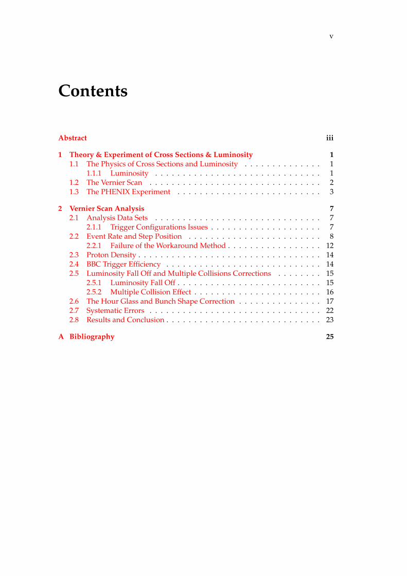
Contents

Abstract iii

1 Theory & Experiment of Cross Sections & Luminosity 11.1 The Physics of Cross Sections and Luminosity . . . . . . . . . . . . . . 1

1.1.1 Luminosity . . . . . . . . . . . . . . . . . . . . . . . . . . . . . . 11.2 The Vernier Scan . . . . . . . . . . . . . . . . . . . . . . . . . . . . . . . 21.3 The PHENIX Experiment . . . . . . . . . . . . . . . . . . . . . . . . . . 3

2 Vernier Scan Analysis 72.1 Analysis Data Sets . . . . . . . . . . . . . . . . . . . . . . . . . . . . . . 7

2.1.1 Trigger Configurations Issues . . . . . . . . . . . . . . . . . . . . 72.2 Event Rate and Step Position . . . . . . . . . . . . . . . . . . . . . . . . 8

2.2.1 Failure of the Workaround Method . . . . . . . . . . . . . . . . . 122.3 Proton Density . . . . . . . . . . . . . . . . . . . . . . . . . . . . . . . . . 142.4 BBC Trigger Efficiency . . . . . . . . . . . . . . . . . . . . . . . . . . . . 142.5 Luminosity Fall Off and Multiple Collisions Corrections . . . . . . . . 15

2.5.1 Luminosity Fall Off . . . . . . . . . . . . . . . . . . . . . . . . . . 152.5.2 Multiple Collision Effect . . . . . . . . . . . . . . . . . . . . . . . 16

2.6 The Hour Glass and Bunch Shape Correction . . . . . . . . . . . . . . . 172.7 Systematic Errors . . . . . . . . . . . . . . . . . . . . . . . . . . . . . . . 222.8 Results and Conclusion . . . . . . . . . . . . . . . . . . . . . . . . . . . . 23

A Bibliography 25

vii

List of Figures

1.1 The PHENIX Detector . . . . . . . . . . . . . . . . . . . . . . . . . . . . 31.2 (a) BBC PMT and Crystal (b) Assembled BBC Module . . . . . . . . . . 4

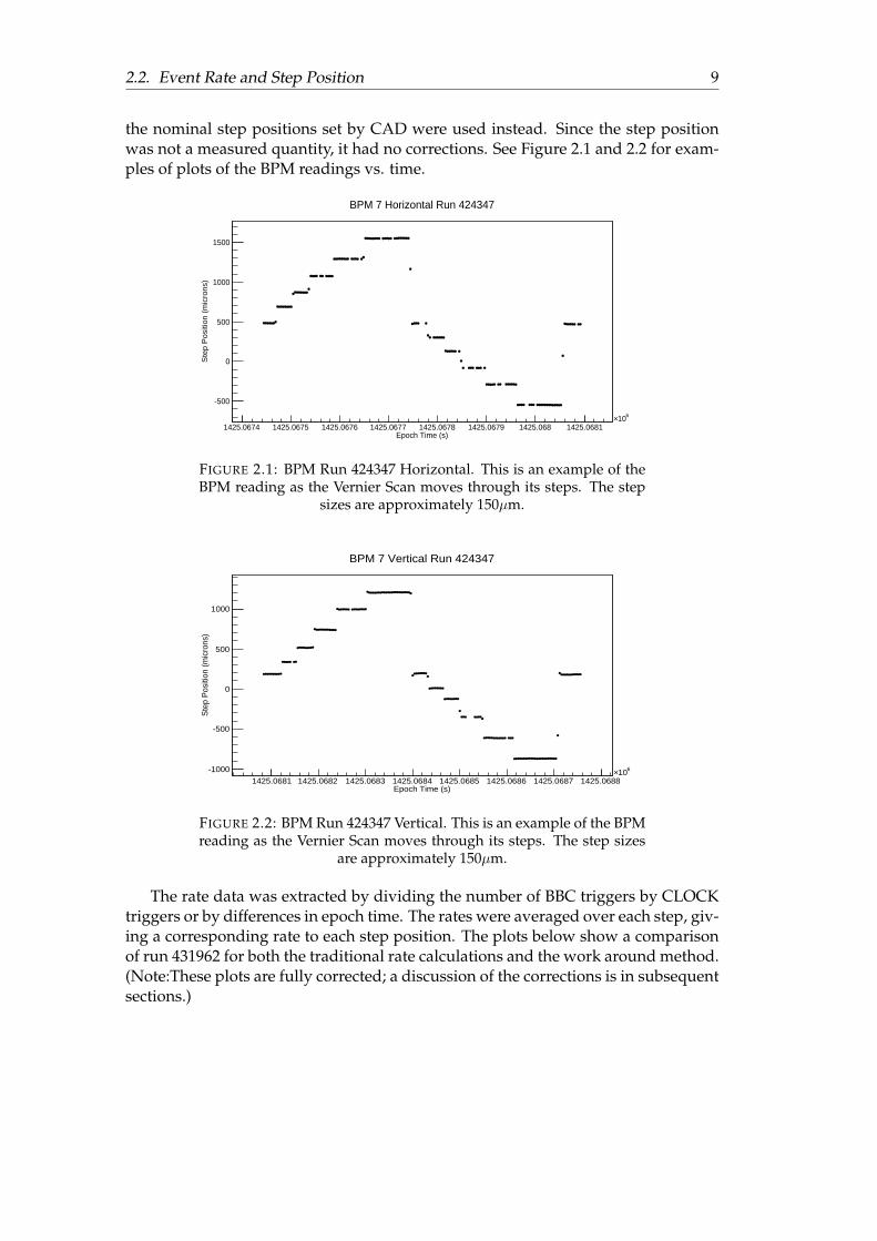
2.1 BPM Run 424347 Horizontal. This is an example of the BPM read-ing as the Vernier Scan moves through its steps. The step sizes areapproximately 150µm. . . . . . . . . . . . . . . . . . . . . . . . . . . . . 9

2.2 BPM Run 424347 Vertical. This is an example of the BPM reading asthe Vernier Scan moves through its steps. The step sizes are approxi-mately 150µm. . . . . . . . . . . . . . . . . . . . . . . . . . . . . . . . . . 9

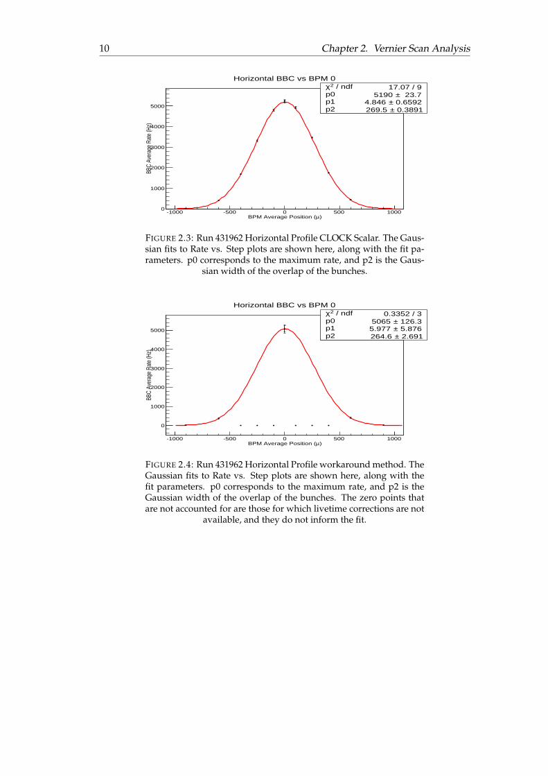
2.3 Run 431962 Horizontal Profile CLOCK Scalar. The Gaussian fits toRate vs. Step plots are shown here, along with the fit parameters. p0corresponds to the maximum rate, and p2 is the Gaussian width ofthe overlap of the bunches. . . . . . . . . . . . . . . . . . . . . . . . . . . 10

2.4 Run 431962 Horizontal Profile workaround method. The Gaussian fitsto Rate vs. Step plots are shown here, along with the fit parameters.p0 corresponds to the maximum rate, and p2 is the Gaussian width ofthe overlap of the bunches. The zero points that are not accounted forare those for which livetime corrections are not available, and they donot inform the fit. . . . . . . . . . . . . . . . . . . . . . . . . . . . . . . . 10

2.5 Run 431962 Vertical Profile CLOCK Scalar. More Gaussian fits wherep0 corresponds to the maximum rate, and p2 is the Gaussian width ofthe overlap of the bunches. . . . . . . . . . . . . . . . . . . . . . . . . . 11

2.6 Run 431962 Vertical Profile workaround. More Gaussian fits wherep0 corresponds to the maximum rate, and p2 is the Gaussian width ofthe overlap of the bunches. The zero points that are not accounted forare those for which livetime corrections are not available, and they donot inform the fit. . . . . . . . . . . . . . . . . . . . . . . . . . . . . . . . 11

2.7 Run 431962 2 Dimensional Profile CLOCK Scalar. This is an exampleof the three dimensional fits which are preferred for extracting themaximum rate. The fit parameters are not shown here. . . . . . . . . . 12

2.8 Run 431962 2 Dimensional Profile workaround. This is an exampleof the three dimensional fits which are preferred for extracting themaximum rate. The fit parameters are not shown here. . . . . . . . . . 12

2.9 Rate andNyNy as a function of bunch crossing number for run 431962.As expected, as one the number of protons goes up, so does the rate . . 13

2.10 The rate and scaled number of protons for the workaround on run431962. The decline in the rate, even as the number of protons in-crease, implies that the livetime correction cannot be applied as abunch average correction, but instead must be considered on a bunchby bunch basis. Since this bunch by bunch livetime information isunavailable, the true rates from the workaround method cannot becalculated. . . . . . . . . . . . . . . . . . . . . . . . . . . . . . . . . . . . 14

viii

2.11 Luminosity Fall Off Run 18776. This figure shows the change in theproduct of the number of protons in each bunch as a function of time.This is due to collisions, beam scrapping, and other effects and is im-portant to insure the correct rate is used. . . . . . . . . . . . . . . . . . 16

2.12 Luminosity Fall Off Run 18721 . . . . . . . . . . . . . . . . . . . . . . . 162.13 Example of Different β∗ [1] . . . . . . . . . . . . . . . . . . . . . . . . . . 182.14 True Bunch Profile (blue) and Three Gaussian Fit (red). The fit pa-

rameters represent the fit to the three Gaussians that sum to give thebunch shape. p0-p2 are the fit parameters left Gaussian, p3-p5 corre-spond to the center Gaussian, and p6-p8 are the right Gaussian. Thethree parameters for each Gauassian are the normalization, mean, andwidth of the Gaussian respectively. . . . . . . . . . . . . . . . . . . . . . 19

2.15 Run 431962 ZDC z Vertex Distribution (a) Max Overlap (b) Min Over-lap. The double peak structure on the left is a result of the structure inz, revealing the effect of a finite β∗ parameter and a nonzero crossingangle. . . . . . . . . . . . . . . . . . . . . . . . . . . . . . . . . . . . . . 20

2.16 Run 431962 Data (blue) Generated (red) (a) Step 0 (b) Step 1 . . . . . . 212.17 Run 431962 Data (blue) Generated (red) (a) Step 2 (b) Step 3. This

shows the correspondence between the generated distribution andthe data for the z distribution of the verticies. . . . . . . . . . . . . . . . 21

2.18 Run 431962 Data (blue) Generated (red) (a) Step 4 (b) Step 5 . . . . . . 222.19 The collection of σBBC values for 431962 with associated error. The fit

was a χ2 fit to a constant function to all the data. The resulting valueis parameter p0. . . . . . . . . . . . . . . . . . . . . . . . . . . . . . . . . 24

2.20 The histogram of all the σBBC values for run 431962. The mean for theGaussian fit to the histogram is consistent with linear fit to the data.

However, given theχ2

NDF= 4, there is not a strong correspondence

between the data and this Gaussian fit. . . . . . . . . . . . . . . . . . . . 24

ix

List of Tables

2.1 Run 15 Vernier Scan Summary . . . . . . . . . . . . . . . . . . . . . . . 72.2 BBC uncorrected and corrected efficiency results. . . . . . . . . . . . . . 15

1

Chapter 1

Theory & Experiment of CrossSections & Luminosity

1.1 The Physics of Cross Sections and Luminosity

1.1.1 Luminosity

Luminosity in particle physics is the proportionality between the rate of a particularprocess, X, and that process’s cross section, σX [1].

dX

dt= L σX

where L is the luminosity, measured in cm−2 s−1 or, since cross sections in parti-cle physics are so small, using millibarns (10−24cm2 = 1mb). The luminosity canbe thought of as characterizing the experimental conditions in a collider. Closelyrelated to the luminosity is the integrated luminosity, L, which is a measure of thenumber of times a process X will occur (NX ) during the integration time period,

NX = L σX

By checking a dataset for the number of events X, it is therefore possible to extractthe cross section of any process X that occurs. In particle physics experiments, theamount of data is often given in terms of integrated luminosity.

In a particle collider, bunches of charge particles are accelerated to high energiesand collided to create interactions. The beams that are collided consist of discretebunches passing through each other, causing one or more collisions for each bunchcrossing. The bunches are modeled as a density of particles moving through space.Locally near the point where the bunches interact, one bunch is considered to bemoving to the left in z, denoted with a + sign, and the other bunch is consideredto be moving to the right in z, denoted with a - sign. The bunches have a time in-dependent 3D structure, where the time dependence translates the bunches in theirrespective directions in the z dimension. A first order expression can be derivedfor the luminosity by assuming the bunch shapes are uncorrelated in all dimensionsand the collisions are head on. The luminosity is treated as the overlap integral oftwo arbitrary density functions, representing the colliding bunches, that depend onx,y,z, and t. The second important assumption about the structure of the bunchesis to assume the density is a product of a Gaussian in all dimensions. This implies,that for the ± bunch, the density can be denoted as ρ± and depends on the number

2 Chapter 1. Theory & Experiment of Cross Sections & Luminosity

of protons in the bunch N±, and the Gaussian width in each dimension σ′x, y z where

ρ± =N±√

(2π)3σ′zσ′xσ′y

e(−x

2

2σ′x− y2

2σ′y− (z±ct)2

2σ′z)

The general overlap integral depends only on the densities of the bunches, thebunch crossing frequency f0, and the number of bunches in the beam Nb. It is givenby,

L = 2f0Nb

∫∫∫∫ ∞−∞

ρ+(x, y, z, ct)ρ−(x, y, z, ct) dx dy dz cdt

where the factor of two is a result of the assumption of head on relativistic collisions.Using the ρ± with a 3D Gaussian and integrating over each dimension, a final,

first order formula for the luminosity is obtained,

L =N+N−f0Nb

4πσ′xσ′y

1.2 The Vernier Scan

Given the important role luminosity plays in determining cross sections, it is impor-tant to characterize it experimentally. This is often done at colliders using a proce-dure known as the Vernier Scan. Originally proposed in 1968 by physicist SimoneVan der Meer, the Vernier Scan has long been the standard for measuring luminos-ity at RHIC, as well as the Large Hadron Collider and other, earlier accelerators.The total luminosity available to an experiment is determined by the minimum biastrigger, which is effectively the condition to begin recording data into the Data Ac-quisition System (DAQ). For a given experiment, a minimum bias detector is oftenused as a luminosity counter. The minimum bias trigger (MB) has a cross section,σMB , the fraction of the total cross section as seen by the minimum bias trigger. Forany physics data set, integrated luminosity is found by the relation,

L =NMB

σMB

where σMB is the quantity determined by the Vernier Scan analysis, and it comesfrom another, similar expression using the instantaneous luminosity and collisionrate,

σMB =RMB

LMBHere, LMB is the luminosity detected by the minimum bias trigger, and RMB is

the collision rate seen by the same MB trigger. LMB is equal to Ldelivered ∗εMB wherethe former is the delivered luminosity and the latter is the minimum bias triggerefficiency.

The collision rate is measured by looking at the ratio of the number of minimumbias triggers over time. The delivered luminosity is calculated from the Vernier Scananalysis:

Ldelivered = f0N+N−4πσx′σy′

as derived above. The parameters σx′ and σy′ are determined via the Vernier Scan.The Vernier scan procedure consists in scanning one beam across the other in

discreet steps, measuring the collision rate at each step position. This enables the

1.3. The PHENIX Experiment 3

measurement of the width of the convolution of the two bunches, in the x-y plane,by looking at the distribution in rate vs. position space. The number of protons ismeasured directly by using an induction detector that measures the charge in thebunch and converting that to a number of protons.

Given the nature of the Vernier Scan, the direct values of σx′ and σy′ are notfound, and instead the overlap width in each dimension is found. Since the widthsare considered to be Gaussian and equivalent for both bunches, the overlap of thebeams is considered to be an overlap as a function of time of two Gaussians with asimple relation between their widths, σx(y) =

√2 ∗ σx(y)′. This leaves a final lumi-

nosity formula in terms of known or observable parameters:

Ldelivered = f0N+N−2πσxσy

1.3 The PHENIX Experiment

The Pioneering High Energy Nuclear Interaction eXperiment (PHENIX) is a gen-eral purpose detector located at the Relativistic Heavy Ion Collider (RHIC) on thecampus of Brookhaven National Labs (BNL) [2]. PHENIX was commissioned tostudy both hot nuclear matter, the quark gluon plasma, and the proton spin prob-lem. Like all similar collider experiments, a large component of the physics involvesinvestigating the production cross section of various processes that result from theproton proton collisions. The importance of the Vernier Scan analysis is to enablethe computation of those cross section by calibrating the minimum bias trigger de-tector efficiency to give an accurate measurement of the luminosity. RHIC collidesboth protons as well as heavy ions. This analysis focuses on p+p collisions whichoccurred at a center of mass energy of

√s = 200 GeV.

The PHENIX experiment consists of several detector subsystems including timeof flight detectors, calorimeters, tracking detectors, and a muon system [2]. A schematicdiagram of the detector system is given below in figure 1.1. The main detectors ofinterest in this analysis are the global counters, the Beam Beam Counter (BBC) andthe Zero Degree Calorimeter (ZDC).

FIGURE 1.1: The PHENIX Detector

The BBC’s are a pair of multipurpose detectors, and for the Vernier Scan analy-sis they act as a minimum bias luminosity counter and vertexing detectors [3]. The

4 Chapter 1. Theory & Experiment of Cross Sections & Luminosity

BBC’s each consists of 3 cm quartz radiator crystals that are read out by 64 PMT’s.The detector units are mounted at ±144 cm from the nominal experimental interac-tion point (IP) in the longitudinal direction. They have a coverage in psuedorapidityof 3.0 < |η| < 3.9. The BBCs are able to vertex events using time of flight with a resolu-tion of 52±4 ps, which gives a spacial resolution of 1 cm. Since the BBCs are close tothe IP, the vertexing precision is dependent on the vertex position and the precisiondecreases further from the interaction point. Additionally, since the BBC uses timeof flight for vertexing, if multiple collisions occur in a single bunch crossing, the BBCis unable to distinguish the collisions, leading to the possibility of under countingthe luminosity. This issue is explored in further detail in the analysis section.

FIGURE 1.2: (a) BBC PMT and Crystal (b) Assembled BBC Module

For the purpose of the Vernier Scan and PHENIX in general, the BBC serves asthe minimum bias trigger, and the ultimate parameter of interest is σBBC , whichcorresponds to σMB in the Luminosity equations above. The maximal rate used isthe maximum BBC rate. The luminosity available to the experiment, and thereforeavailable to compute cross sections, is only the luminosity seen by the BBC. For thisreason the BBC serves as PHENIX’s luminosity counter.

The ZDCs are two symmetric hadronic calorimeters located very far from theinteraction point at ±18 m [4]. This enables the ZDCs to detect very low transversemomentum particles, |η| > 6, which is crucial in determining the centrality in heavyion collisions. For the Vernier Scan, the ZDCs serve as a z vertex detector usingtime of flight difference. Due the small geometric acceptance, the ZDCs see veryfew events, limiting the effect of multiple collisions and enabling corrections to BBCdata for effects that depend strongly on the z vertex position. The ZDC’s also seesthe entire interaction region, allowing for corrections to effects that consider scales inthe transverse dimensions that are greater than the BBC’s. The ZDC can determinez vertices to a precision of ±15 cm.

For the Vernier Scan, the ZDCs are used to correct for any longitudinally depen-dent effects in the analysis. Given that all the formulas derived above depend on theapproximation of uncorrelated densities in all dimensions, to correct for this over-sight the true shape of the bunch is later applied as a correction. The ZDC is the onlydetector that can access the entire bunch in the longitudinal (z) dimension, makingit critical to make such z dependent corrections.

Several of the parameters of the Vernier Scan analysis are set or measured by theCollider Accelerator Department (CAD) at BNL and incorporated into this analysis.

1.3. The PHENIX Experiment 5

The number of protons in each bunch in the beam is measured using two separateinduction detectors, the Wall Current Monitor (WCM) and the Direct Current Cur-rent Transformer (DCCT) [5]. These detectors are both induction detectors, readingout a current as the bunches pass through a closed circuit, generating an inductioncurrent. The WCM is a fast detector, giving bunch by bunch readouts of the numberor protons. The DCCT is a slower detector, but it has a lower systematic error andis less sensitive to debunching effects. Both detectors are used to generate the finalvalue for the number of protons in each bunch. The bunch crossing frequency, f0, isset by CAD to be about 78 kHz meaning a particular bunch from one beam crossesa particular bunch from another beam 78 thousand times per second.

7

Chapter 2

Vernier Scan Analysis

The Vernier Scan analysis for PHENIX consists of several distinct experimental tech-niques over several data sets, outlined in the sections below.

2.1 Analysis Data Sets

The Vernier Scan analysis consists of data taken at the end of a 90 minute periodof data collection, known as a run at PHENIX. In order to establish a statisticallysignificant measurement, several data sets are generated over the entire course ofp+p running. The Vernier scans occur for a period of about 15 minutes, with 24 stepstotal. The scan begins with the beams in a maximally overlapped configuration, asthey would be during normal running, then moving outward in steps of between100 and 250 µm. First the horizontal direction was scanned, then the vertical. Asummary table of the scans taken over all of 2015, known as Run 15, is in table 2.1.

Run Fill Comments424347 18721 Run Control Server Failure426254 18776 -431624 18942 Test of Diagonal Scan (Omitted in Analysis)431723 18943 Diagonal and Horizontal/Vertical Scans431942 18952 CLOCK Trigger Enabled

TABLE 2.1: Run 15 Vernier Scan Summary

The Run Control Server failure was a communication issue between the PHENIXcontrol room and the Collider Accelerator control room. This issue did not ulti-mately affect the data collected for run 424347. The diagonal test scan was a proofof concept, in order to more accurately confirm the assumption of Gaussian distri-butions in the x-y plane. However, data collection issues resulting from an incorrecttrigger configuration prevented the diagonal scan from being utilized. The final scanwas taken after the trigger configuration issues were resolved (i.e. the CLOCK trig-ger was enabled).

2.1.1 Trigger Configurations Issues

An unfortunate issue with PHENIX p+p Vernier Scan for Run 15 was the correcttrigger configuration was not enabled except for the last scan. Normally for theVernier Scan, two types of data are used to compute the rates at each displacedstep position, the BBC_MB scalar counts and the CLOCK scalar counts. The formerrecords the number of minimum bias trigger over the course of a run, and the lat-ter is a scaled value of the time. The rates are then calculated by taking the ratio of

8 Chapter 2. Vernier Scan Analysis

the number of BBC_MB scalars and CLOCK scalars, then scaling the CLOCK to re-cover time. However, for the majority of Vernier Scan data sets in Run 15, excluding431962, the CLOCK trigger was not enabled in the DAQ. Instead of simply dividingtwo trigger counts, a raw number of cumulative triggers and an associated EPOCHtime stamp was used to compute rates by taking the difference in counts betweentwo sequential steps and dividing by the difference in epoch time. Unfortunately,the rates extracted via this method proved to be unreliable, making it impossible toperform the full Vernier scan procedure on the majority of the data sets. However,certain aspects of the scan, in particular the values of the BBC trigger efficiency, wereextracted from each run, since it did not require the workaround method in the sameway the rates did.

The main issue with the workaround method was that the data needed to becorrected for livetime effects. The livetime of the DAQ is the fraction of time that theDAQ is taking data. When an event arrives at the DAQ, no more data is analyzeduntil the current level 0 analysis is completed. Therefore, while the DAQ is busy,some data is not accepted. However, scalar counters still record the number of totaltriggers, and these scalars are not overwhelmed by the data taking rate. Therefore,the livetime is the number of scalars accumulated when the DAQ is live dividedby the total number of scalars. The livetime changes dramatically and nonlinearlybetween Vernier Scan steps, because the data collection rate can greatly vary givenhow much of the beams are overlapping. Since the beam widths are Gaussian, alinear change in beam overlap can cause a dramatic drop in the rate. As the ratefalls, the livetime rises because the DAQ is busy more often.

The correction that was attempted depended on data packets that occurred ap-proximately every 30 s. Since the Vernier scan step duration lasted between 30sand 1 minute, there was the possibility that two data packets would be containedwithin a single steps, while other steps had only one or zero packets. Since the dif-ference between two data packets was needed to compute the livetime for a step,only those steps which had two data packets could be utilized. Enough steps hadtwo data packets such that a beam profile was able to be extracted from each run.Unfortunately, the data was still unusable due to issues with the rate calculation, asis explained in the subsection on the livetime correction in the next section.

2.2 Event Rate and Step Position

The data that is generated specifically for the Vernier Scan relates to the transversebeam profiles, σx(y). The physical scan that occurs is the process of sweeping onebeam across the other at discrete steps in the transverse (xy) plane, generating a datapoint in Rate vs. Position space. The rate data for a single transverse dimension areplotted first separately in one dimension, then the rate vs. position is plotted forthe entire transverse plane in a two dimensional plot. The 1D plots are fit with asimple Gaussian function, with the normalization equating to Rmax and the widthcorresponding to σx(y). The 2D case is similarly fit with the product of a Gaussianfunction in x and in y with the fit parameters corresponding to the same quantitiesas the 1D case. While the fit parameter values for the 1 and 2 dimensional fits differonly by 1%, the 2D fit is preferred given that the beam may not return to exactmaximal overlap in later steps during the scan.

The step position has, in previous years, been taken from the CAD’s Beam Po-sition Monitors which record the beam location in the x-y plane. However, givenknown and possible issues in the BPM’s measurements that are difficult to calibrate,

2.2. Event Rate and Step Position 9

the nominal step positions set by CAD were used instead. Since the step positionwas not a measured quantity, it had no corrections. See Figure 2.1 and 2.2 for exam-ples of plots of the BPM readings vs. time.

Epoch Time (s)1425.0674 1425.0675 1425.0676 1425.0677 1425.0678 1425.0679 1425.068 1425.0681

610×

Ste

p P

osi

tion

(m

icro

ns)

-500

0

500

1000

1500

BPM 7 Horizontal Run 424347

FIGURE 2.1: BPM Run 424347 Horizontal. This is an example of theBPM reading as the Vernier Scan moves through its steps. The step

sizes are approximately 150µm.

Epoch Time (s)1425.0681 1425.0682 1425.0683 1425.0684 1425.0685 1425.0686 1425.0687 1425.0688

610×

Ste

p P

ositi

on (

mic

rons

)

-1000

-500

0

500

1000

BPM 7 Vertical Run 424347

FIGURE 2.2: BPM Run 424347 Vertical. This is an example of the BPMreading as the Vernier Scan moves through its steps. The step sizes

are approximately 150µm.

The rate data was extracted by dividing the number of BBC triggers by CLOCKtriggers or by differences in epoch time. The rates were averaged over each step, giv-ing a corresponding rate to each step position. The plots below show a comparisonof run 431962 for both the traditional rate calculations and the work around method.(Note:These plots are fully corrected; a discussion of the corrections is in subsequentsections.)


)µBPM Average Position (-1000 -500 0 500 1000

BBC

Aver

age

Rate

(Hz)

0

1000

2000

3000

4000

5000

/ ndf 2χ 17.07 / 9p0 23.7± 5190 p1 0.6592± 4.846 p2 0.3891± 269.5

/ ndf 2χ 17.07 / 9p0 23.7± 5190 p1 0.6592± 4.846 p2 0.3891± 269.5

Horizontal BBC vs BPM 0

FIGURE 2.3: Run 431962 Horizontal Profile CLOCK Scalar. The Gaus-sian fits to Rate vs. Step plots are shown here, along with the fit pa-rameters. p0 corresponds to the maximum rate, and p2 is the Gaus-

sian width of the overlap of the bunches.


BBC

Aver

age

Rate

(Hz)

0

1000

2000

3000

4000

5000

/ ndf 2χ 0.3352 / 3p0 126.3± 5065 p1 5.876± 5.977 p2 2.691± 264.6

/ ndf 2χ 0.3352 / 3p0 126.3± 5065 p1 5.876± 5.977 p2 2.691± 264.6

Horizontal BBC vs BPM 0

FIGURE 2.4: Run 431962 Horizontal Profile workaround method. TheGaussian fits to Rate vs. Step plots are shown here, along with thefit parameters. p0 corresponds to the maximum rate, and p2 is theGaussian width of the overlap of the bunches. The zero points thatare not accounted for are those for which livetime corrections are not

available, and they do not inform the fit.



BBC

Aver

age

Rate

(Hz)

0

1000

2000

3000

4000

5000

/ ndf 2χ 47.96 / 8p0 23.45± 5158 p1 0.6687± 8.443 p2 0.3936± 254.2

/ ndf 2χ 47.96 / 8p0 23.45± 5158 p1 0.6687± 8.443 p2 0.3936± 254.2

Vertical BBC vs BPM

FIGURE 2.5: Run 431962 Vertical Profile CLOCK Scalar. More Gaus-sian fits where p0 corresponds to the maximum rate, and p2 is the

Gaussian width of the overlap of the bunches.


BBC

Aver

age

Rate

(Hz)

0

1000

2000

3000

4000

5000

/ ndf 2χ 0.443 / 3p0 106± 5210 p1 5.511± 20.5 p2 2.738± 254.6

/ ndf 2χ 0.443 / 3p0 106± 5210 p1 5.511± 20.5 p2 2.738± 254.6

Vertical BBC vs BPM

FIGURE 2.6: Run 431962 Vertical Profile workaround. More Gaus-sian fits where p0 corresponds to the maximum rate, and p2 is theGaussian width of the overlap of the bunches. The zero points thatare not accounted for are those for which livetime corrections are not

available, and they do not inform the fit.


FIGURE 2.7: Run 431962 2 Dimensional Profile CLOCK Scalar. Thisis an example of the three dimensional fits which are preferred forextracting the maximum rate. The fit parameters are not shown here.

FIGURE 2.8: Run 431962 2 Dimensional Profile workaround. Thisis an example of the three dimensional fits which are preferred forextracting the maximum rate. The fit parameters are not shown here.

2.2.1 Failure of the Workaround Method

An unfortunate consequence of the incorrect scalars being enabled at the time datawas taken was that the rates were not able to be corrected for livetime on a bunch bybunch basis. A naive assumption would imply that each crossing of bunches wouldhave similar numbers of protons and densities which would lead to similar rates.Upon investigating systematic effects, however, the livetime correction introducedsystematic effects into the data that varied with the bunch crossing. In particular, therate with the livetime correction tended to fall as the number of protons increases.Given that the bunch widths are constant (with only statistical error) the rates shouldincrease as the number of particles increases.

During the run for which the CLOCK scalar was available, this was the case, andsince the final value of σBBC has the relationship,

σBBC ∝R

NbNy


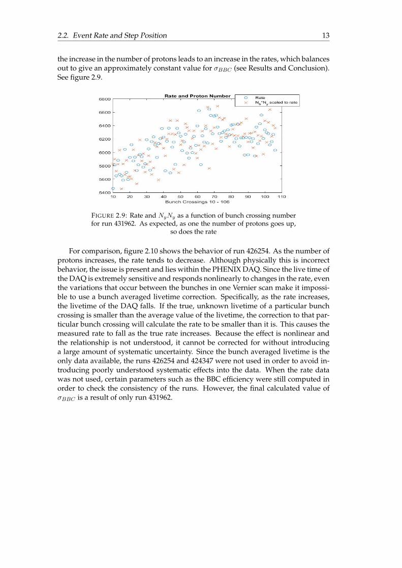
the increase in the number of protons leads to an increase in the rates, which balancesout to give an approximately constant value for σBBC (see Results and Conclusion).See figure 2.9.

FIGURE 2.9: Rate and NyNy as a function of bunch crossing numberfor run 431962. As expected, as one the number of protons goes up,

so does the rate

For comparison, figure 2.10 shows the behavior of run 426254. As the number ofprotons increases, the rate tends to decrease. Although physically this is incorrectbehavior, the issue is present and lies within the PHENIX DAQ. Since the live time ofthe DAQ is extremely sensitive and responds nonlinearly to changes in the rate, eventhe variations that occur between the bunches in one Vernier scan make it impossi-ble to use a bunch averaged livetime correction. Specifically, as the rate increases,the livetime of the DAQ falls. If the true, unknown livetime of a particular bunchcrossing is smaller than the average value of the livetime, the correction to that par-ticular bunch crossing will calculate the rate to be smaller than it is. This causes themeasured rate to fall as the true rate increases. Because the effect is nonlinear andthe relationship is not understood, it cannot be corrected for without introducinga large amount of systematic uncertainty. Since the bunch averaged livetime is theonly data available, the runs 426254 and 424347 were not used in order to avoid in-troducing poorly understood systematic effects into the data. When the rate datawas not used, certain parameters such as the BBC efficiency were still computed inorder to check the consistency of the runs. However, the final calculated value ofσBBC is a result of only run 431962.


FIGURE 2.10: The rate and scaled number of protons for theworkaround on run 431962. The decline in the rate, even as the num-ber of protons increase, implies that the livetime correction cannotbe applied as a bunch average correction, but instead must be con-sidered on a bunch by bunch basis. Since this bunch by bunch live-time information is unavailable, the true rates from the workaround

method cannot be calculated.

2.3 Proton Density

The total intensity of the beam is the number of protons in one beam, i.e. all thebunches of protons traveling one direction, multiplied by the number of protons inthe other beam (called arbitrarily ’blue’ and ’yellow’ in PHENIX). This is brokendown for each bunch crossing to find a density for each bunch in both beams. Theparameter comes directly from CAD measurements generated by the Wall CurrentMonitor (WCM). The wall current monitor takes readings for each bunch in timebins averaged over one second. The values for Nb and Ny are taken from a periodof approximately 100 seconds prior to the beginning of the Vernier Scan, averagedover time and used in the final computation of σBBC . However, the WCM measure-ments are not particularly accurate and the detector has a relatively high amount ofsystematic uncertainty ( 2%) as it is sensitive to debunching effects. Therefore, eachWCM reading is normalized with respect to another proton counter, the Direct Cur-rent Current Transformer (DCCT). Since the DCCT acts over a longer timescale, it isless sensitive to debunching than the WCM, and it has a smaller degree of systematicuncertainty ( 0.2%). The normalization consists of averaging the WCM and DCCTreadings over the same 100 second prior to the scan (t) and over all bunches for theWCM (bunches). Then, for the ith bunch:

Ni,b(y) =

∑tDCCT∑

t

∑bunches

WCMWCMi,b(y)

This provides an accurate accounting of the number of protons in each bunch.

2.4 BBC Trigger Efficiency

The luminosity sampled by the minimum bias trigger is needed for the calculationof the BBC cross section.

2.5. Luminosity Fall Off and Multiple Collisions Corrections 15

LBBC = Ldelivered × εMBBBC

where εMBBBC is the fraction of the vertex distribution triggered on by the minimum

bias trigger of the BBC. Different BBC triggers serve different functions, and theminimum bias trigger has a range of approximately 30 cm. The BBC_wide triggerhas a larger range of coverage in z, extending from ±144 cm. The efficiency of theminimum bias trigger is measured by dividing the number of triggers that occurinside the BBC minimum bias trigger’s range in coincidence with the BBC widetrigger, which covers a wider region, by the total number of wide triggers for theBBC according to the equation,

εMBBBC =

NMB+wideBBC

NwideBBC

.

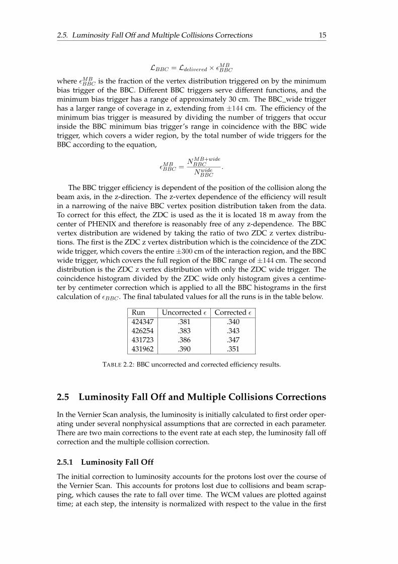
The BBC trigger efficiency is dependent of the position of the collision along thebeam axis, in the z-direction. The z-vertex dependence of the efficiency will resultin a narrowing of the naive BBC vertex position distribution taken from the data.To correct for this effect, the ZDC is used as the it is located 18 m away from thecenter of PHENIX and therefore is reasonably free of any z-dependence. The BBCvertex distribution are widened by taking the ratio of two ZDC z vertex distribu-tions. The first is the ZDC z vertex distribution which is the coincidence of the ZDCwide trigger, which covers the entire ±300 cm of the interaction region, and the BBCwide trigger, which covers the full region of the BBC range of ±144 cm. The seconddistribution is the ZDC z vertex distribution with only the ZDC wide trigger. Thecoincidence histogram divided by the ZDC wide only histogram gives a centime-ter by centimeter correction which is applied to all the BBC histograms in the firstcalculation of εBBC . The final tabulated values for all the runs is in the table below.

Run Uncorrected ε Corrected ε424347 .381 .340426254 .383 .343431723 .386 .347431962 .390 .351

TABLE 2.2: BBC uncorrected and corrected efficiency results.

2.5 Luminosity Fall Off and Multiple Collisions Corrections

In the Vernier Scan analysis, the luminosity is initially calculated to first order oper-ating under several nonphysical assumptions that are corrected in each parameter.There are two main corrections to the event rate at each step, the luminosity fall offcorrection and the multiple collision correction.

2.5.1 Luminosity Fall Off

The initial correction to luminosity accounts for the protons lost over the course ofthe Vernier Scan. This accounts for protons lost due to collisions and beam scrap-ping, which causes the rate to fall over time. The WCM values are plotted againsttime; at each step, the intensity is normalized with respect to the value in the first


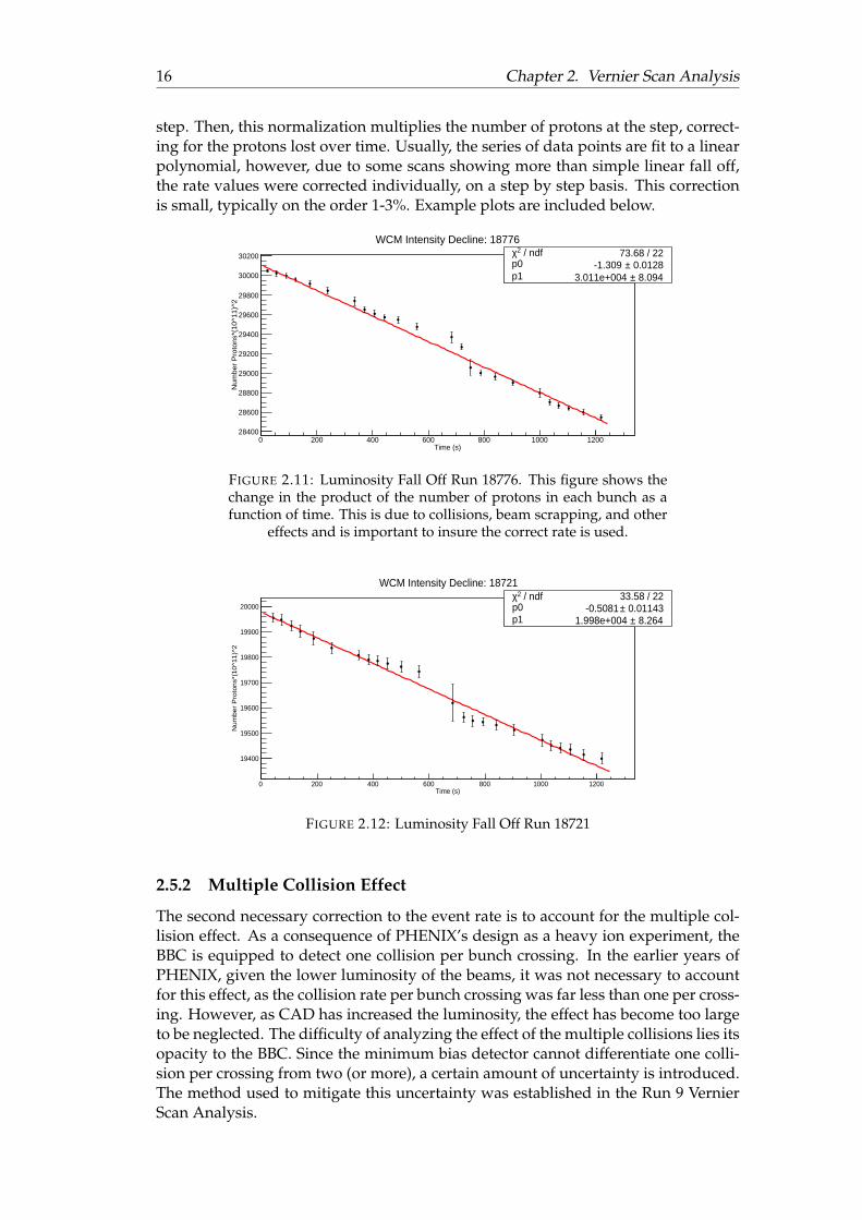
step. Then, this normalization multiplies the number of protons at the step, correct-ing for the protons lost over time. Usually, the series of data points are fit to a linearpolynomial, however, due to some scans showing more than simple linear fall off,the rate values were corrected individually, on a step by step basis. This correctionis small, typically on the order 1-3%. Example plots are included below.

Time (s)0 200 400 600 800 1000 1200

Num

ber

Pro

tons

*(10

^11)

^2

28400

28600

28800

29000

29200

29400

29600

29800

30000

30200 / ndf 2χ 73.68 / 22p0 0.0128± -1.309 p1 8.094± 3.011e+004

/ ndf 2χ 73.68 / 22p0 0.0128± -1.309 p1 8.094± 3.011e+004

WCM Intensity Decline: 18776

FIGURE 2.11: Luminosity Fall Off Run 18776. This figure shows thechange in the product of the number of protons in each bunch as afunction of time. This is due to collisions, beam scrapping, and other

effects and is important to insure the correct rate is used.

Time (s)0 200 400 600 800 1000 1200

Num

ber

Pro

tons*

(10^1

1)^

2

19400

19500

19600

19700

19800

19900

20000 / ndf 2χ 33.58 / 22

p0 0.01143± -0.5081 p1 8.264± 1.998e+004

/ ndf 2χ 33.58 / 22p0 0.01143± -0.5081 p1 8.264± 1.998e+004

WCM Intensity Decline: 18721

FIGURE 2.12: Luminosity Fall Off Run 18721

2.5.2 Multiple Collision Effect

The second necessary correction to the event rate is to account for the multiple col-lision effect. As a consequence of PHENIX’s design as a heavy ion experiment, theBBC is equipped to detect one collision per bunch crossing. In the earlier years ofPHENIX, given the lower luminosity of the beams, it was not necessary to accountfor this effect, as the collision rate per bunch crossing was far less than one per cross-ing. However, as CAD has increased the luminosity, the effect has become too largeto be neglected. The difficulty of analyzing the effect of the multiple collisions lies itsopacity to the BBC. Since the minimum bias detector cannot differentiate one colli-sion per crossing from two (or more), a certain amount of uncertainty is introduced.The method used to mitigate this uncertainty was established in the Run 9 VernierScan Analysis.

2.6. The Hour Glass and Bunch Shape Correction 17

The first important equation describes the true rate [6],

Rtrue = µ ∗ ε2side ∗ εBBC ∗ f

where µ is the average number of collisions in a bunch crossing, εside is the single sideefficiency of the BBC, εBBC is the trigger efficiency of the BBC discussed previously,and f is the bunch crossing frequency. Since, ideally, the two efficiencies and f aremachine parameters, knowing µ for a bunch crossing would enable the true rateto be calculated. However, µ cannot be determined directly. Instead, from Poissonstatistics the observed rate is expected to be,

Rpred = εBBC [1− 2e−2µεside + e−µεside(2−εside)]

Since we understand what the observed rate should be from that formula and µis the only unknown parameter, by iteratively minimizing the difference between theactual observed rate R and the predicted observed rate Rpred we obtain the correctµ. To do this, Newton’s method of root finding is used on the function f(µ) = R −Rpred. When the difference between two subsequent iterations is zero, the functionis considered to be minimized, and the value of µ found is used in the true rateequation. A value of µ is found at each step position, giving a change of between5-10% at maximal overlap, and <1% at minimal overlap.

It is assumed in this analysis that differences in north and south hit probabilitiesare small, and a nominal value for εside = .79 is used for this analysis, as establishedin Run 9. In order to compensate for possible fluctuations, εside is varied by ±3%which accounts for systematic error in the multiple collisions correction. This erroris motivated by the understanding that εside is not accurately known.

2.6 The Hour Glass and Bunch Shape Correction

In the simplest cases, luminosity is calculated as it was described in the first chapter,

Ldelivered = f0NbNy

2πσxσy

However, this formula does not account for the possible effects of the z dependenceof the bunch structure. The simple formula that is used to approximate luminos-ity per bunch comes from the parent formula, which integrates over the collidingbunches in x, y, z, and ct:

L = 2f0

∫∫∫∫ ∞−∞

ρ+(x, y, z, ct)ρ−(x, y, z, ct) dx dy dz cdt

Here, ρ± is the structure of each bunch and, assuming Gaussian distributions in x, y,and z±ct,

ρ±(x, y, z ± ct) =N±

(2π)3/2σx′(z)σy′(z)σ(z)e( −x

2

2σx′(z)+ −y2

2σy ′(z)+−(z±ct)2

2σz)

The dependence of the x-y plane on the longitudinal dimension is explainedphysically by the structure of the focusing magnets near the IP. Given that mag-net can optimally focus the beam at one point, the IP, the density in x and y dependson how close the transverse plane is to z = 0. To account for the dependence of σx(y)


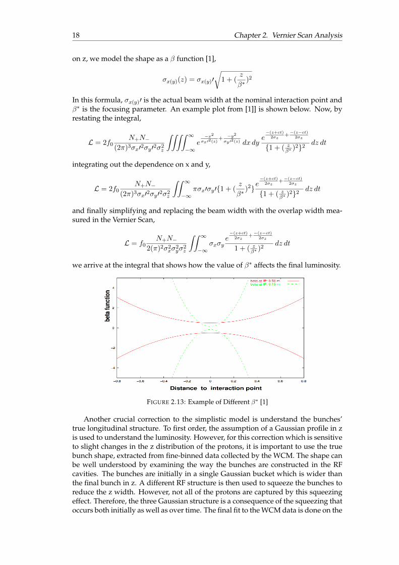
on z, we model the shape as a β function [1],

σx(y)(z) = σx(y)′√1 + (

z

β∗)2

In this formula, σx(y)′ is the actual beam width at the nominal interaction point andβ∗ is the focusing parameter. An example plot from [1]] is shown below. Now, byrestating the integral,

L = 2f0N+N−

(2π)3σx′2σy′2σ2z

∫∫∫∫ ∞−∞

e−x2

σx′2(z)+ −y2

σy ′2(z) dx dye−(z+ct)

2σz+−(z−ct)

2σz

{1 + ( zβ∗ )2}2

dz dt

integrating out the dependence on x and y,

L = 2f0N+N−

(2π)3σx′2σy′2σ2z

∫∫ ∞−∞

πσx′σy′{1 + (z

β∗)2}e

−(z+ct)2σz

+−(z−ct)

2σz

{1 + ( zβ∗ )2}2

dz dt

and finally simplifying and replacing the beam width with the overlap width mea-sured in the Vernier Scan,

L = f0N+N−

2(π)2σ2xσ2yσ

2z

∫∫ ∞−∞

σxσye−(z+ct)

2σz+−(z−ct)

2σz

1 + ( zβ∗ )2

dz dt

we arrive at the integral that shows how the value of β∗ affects the final luminosity.

FIGURE 2.13: Example of Different β∗ [1]

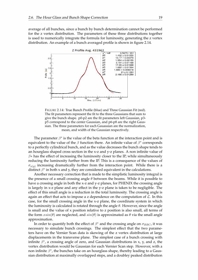
Another crucial correction to the simplistic model is understand the bunches’true longitudinal structure. To first order, the assumption of a Gaussian profile in zis used to understand the luminosity. However, for this correction which is sensitiveto slight changes in the z distribution of the protons, it is important to use the truebunch shape, extracted from fine-binned data collected by the WCM. The shape canbe well understood by examining the way the bunches are constructed in the RFcavities. The bunches are initially in a single Gaussian bucket which is wider thanthe final bunch in z. A different RF structure is then used to squeeze the bunches toreduce the z width. However, not all of the protons are captured by this squeezingeffect. Therefore, the three Gaussian structure is a consequence of the squeezing thatoccurs both initially as well as over time. The final fit to the WCM data is done on the


average of all bunches, since a bunch by bunch determination cannot be performedfor the z vertex distribution. The parameters of these three distributions togetheris used to numerically integrate the formula for luminosity, generating the z vertexdistribution. An example of a bunch averaged profile is shown in figure 2.14.

FIGURE 2.14: True Bunch Profile (blue) and Three Gaussian Fit (red).The fit parameters represent the fit to the three Gaussians that sum togive the bunch shape. p0-p2 are the fit parameters left Gaussian, p3-p5 correspond to the center Gaussian, and p6-p8 are the right Gaus-sian. The three parameters for each Gauassian are the normalization,

mean, and width of the Gaussian respectively.

The parameter β∗ is the value of the beta function at the interaction point and isequivalent to the value of the β function there. An infinite value of β∗ correspondsto a perfectly cylindrical bunch, and as the value decreases the bunch shape tends toan hourglass shaped cross section in the x-z and y-z planes. A non infinite value ofβ∗ has the effect of increasing the luminosity closer to the IP, while simultaneouslyreducing the luminosity further from the IP. This is a consequence of the values ofσx(y) increasing dramatically further from the interaction point. While there is adistinct β∗ in both x and y, they are considered equivalent in the calculations.

Another necessary correction that is made to the simplistic luminosity integral isthe presence of a small crossing angle θ between the beams. While it is possible tohave a crossing angle in both the x-z and y-z planes, for PHENIX the crossing angleis largely in x-z plane and any effect in the y-z plane is taken to be negligible. Theeffect of this small angle is a reduction in the total luminosity. The crossing angle isagain an effect that acts to impose a z dependence on the computation of L. In thiscase, for the small crossing angle in the x-z plane, the coordinate system in whichthe luminosity is calculated is rotated through the angle θ. However, since the angleis small and the value of x position relative to z position is also small, all terms ofthe form xsin(θ) are neglected, and sin(θ) is approximated as θ via the small angleapproximation.

In order to quantify both the effect of β∗ and the crossing angle on σBBC , it wasnecessary to simulate bunch crossings. The simplest effect that the two parame-ters have on the Vernier Scan data is skewing of the z vertex distribution at largedisplacements in the transverse plane. The simplest case of a bunch crossing withinfinite β∗, a crossing angle of zero, and Gaussian distributions in x, y, and z, thevertex distribution would be Gaussian for each Vernier Scan step. However, with anon infinite β∗, the bunches take on an hourglass shape, thereby leading to a Gaus-sian distribution at maximally overlapped steps, and a doubley peaked distribution


at a greater transverse displacement. Secondly, the crossing angle causes a skew inthe double peak structure of the z vertex distribution at minimal overlap; the angleforces one side of the interaction region to have a greater overlap of bunches, therebycausing more collisions on that side. This effect is easily observed by examining theZDC z distribution of verticies data node in the Vernier Scan output.

(A) (B)

FIGURE 2.15: Run 431962 ZDC z Vertex Distribution (a) Max Overlap(b) Min Overlap. The double peak structure on the left is a result ofthe structure in z, revealing the effect of a finite β∗ parameter and a

nonzero crossing angle.

In order to determine the value of β∗ and the crossing angle, a numerical dis-tribution of the luminous region is generated from the overlap integrals, such thattheir z vertex distribution can be matched to data. The ZDC z vertex distributionwas chosen because some of the effects spill over beyond the ±144 cm where theBBC’s are located, and the ZDC’s efficiency is not z dependent. The numerical inte-gration derives its z verticies directly from numerically integrating the full form ofthe luminosity equation, including the effects of β∗ and crossing angle, as well as thetrue z structure of the bunches obtained from finely binned WCM data, integratingover x, y, and z to generate a single distribution in t. The distribution is normalized,and a distribution in z is generated by summing over all the bins in t. The z bins ofthe distribution are smeared for ZDC resolution effects with a Gaussian where theposition resolution is σ=15 cm.

The generated histogram is then compared to the data histogram, and β∗ and thecrossing angle are adjusted to converge to the best fit. The same program computes ascaled value of luminosity, which is first done with the physical values of the param-eters found by comparison, then the computation of luminosity is repeated for thefirst order approximation of infinite β∗ and zero crossing angle. A normalization, Sis then computed by dividing the luminosity with physical values by the luminositywith first order values,

S =LphysicalLfirst order

Given the possibility of systematic errors in the simulation, the computed value ofthe simulation luminosity is not considered be accurate enough to be used. There-fore, the eventual calculation of the delivered luminosity is modified to,

Ldelivered = SLfirst order


Example plots of the data and generated distribution are below. The steps arenumbered from 0 to 11, and with 0 being the maximally overlapped configuration,5 being minimally overlapped, 6 returning to max overlap and 11 minimally over-lapped. All generated distributions have a β∗ = 90 cm and θ = .06 mrad.

(A) (B)

FIGURE 2.16: Run 431962 Data (blue) Generated (red) (a) Step 0 (b)Step 1

(A) (B)

FIGURE 2.17: Run 431962 Data (blue) Generated (red) (a) Step 2 (b)Step 3. This shows the correspondence between the generated distri-

bution and the data for the z distribution of the verticies.

The evolution of the structure of the z vertex distribution is a consequence of thegeometry of the interaction region. The finite β∗ causes the double peak structurefor the minimally overlapped steps, whereas the crossing angle causes the asym-metry of the distribution. Ultimately, the complexity of the bunch structure andthe coarseness of the generated distribution make it impossible to use the generateddistribution as an absolute measurement of the two parameters. Therefore, the sim-ulation is used to confirm with an uncertainty of approximately ten percent, thatCAD’s quoted values of β∗ and the crossing angle are correct.


(A) (B)

FIGURE 2.18: Run 431962 Data (blue) Generated (red) (a) Step 4 (b)Step 5

2.7 Systematic Errors

There were several sources of systematic error identified in the various steps of theVernier Scan analysis. The final computed quantity, σBBC , can be broken down interms of the parameters that comprise it.

σBBC =RmaxLBBC

=Rmax

εtrigSLdelivered= Rmax

2πσxσyNbNyf0εtrigS

In order to compute a final systematic error, the systematic error for each param-eter is found separately, and errors are then propagated according to the formula:

δσBBC = σBBC

√√√√ n∑i=1

(δp

p)2

Here, p is any paramter and δp is its associated systematic error. For the parame-ters that had identifiable sources of error, the systematic error was found first forthe uncorrected value, then for each correction individually. The final systematicerror on the parameter was the sum in quadrature of its uncorrected error and eachcorrection’s error.

The error estimation begins by looking at systematic errors of Rmax. Since theuncorrected measurement ofRmax is simply BBC Trigger counts divided by CLOCKtrigger or epoch time, it is assumed to be free of systematic error. Additionally,the systematic error resulting from the Luminosity fall off correction was neglectedgiven the correction’s 1% change and the 2% systematic on the WCM. To account forpossible errors in the step positions, the Rate vs. Step plots were generated usingfirst the CAD set steps, then the BPM measured steps. The difference in the value ofRmax, about 1.5%, was used as additional systematic error. The multiple collisionseffect did introduce systematic error into the determination of Rmax as discussed inthe rate section. The multiple collisions error varies with displacement of the beam,and is averaged over all steps for each bunch crossing. The fractional error for thecorrected rate was around 3%.

2.8. Results and Conclusion 23

The systematic error on the intensity comes directly from the CAD quoted valuesof the systematic errors for the WCM and DCCT readings. CAD quotes the system-atic error for the WCM at 2% and the DCCT at .2%. Given that Nb(y) is normalizedby the DCCT, the associated error, minus an approximated correlation, gives a finalerror of approximately .8%.

The error that resulted from σx and σy were computed as combinations of therate error and the step position error. The rate error came by extracting values ofσx(y) from the uncorrected rate, then taking the fit parameter using the correct rate.The difference between the two was used as the error, and was approximately .5%.The error that came from uncertainty on step positions was computed similarly tothe step position error on rate. The fit parameters were taken first using CAD setsteps, then using BPM measured steps, and the difference was the possible error.This error was .7% for σx and .5% for σy.

The systematic error in the parameter εBBC was taken to be the square root ofthe variance of all of the values of εBBC for all Vernier scans. The final value was forthe error was .00439, which makes the relative error on the order of one percent, andspecifically for 431962, the fractional error was 1.2%.

The correction of β∗ and the crossing angle had a high relative systematic errorsince the generated distributions and data plots were not matched to a high degreeof precision. The spread around the best value that still appeared to give a tolera-ble z vertex distribution were used to compute correction factors. Once the factorswere computed, the difference between them was used as an absolute error on thecorrection, and the fractional error was around 10%.

2.8 Results and Conclusion

Using only run 431962, the final value of BBC min bias detector cross section was,

σBBC = 30.0± 1.8± 3.4 mb

where the first error is statistical and the second is systematic. The overall statisti-cal error is simply the standard deviation of the bunches, and the overall systematicerror is the result of error propagation as defined in the previous section. The sys-tematic error was approximately 11.3%, where the largest contribution comes fromuncertainty in the β∗ correction.

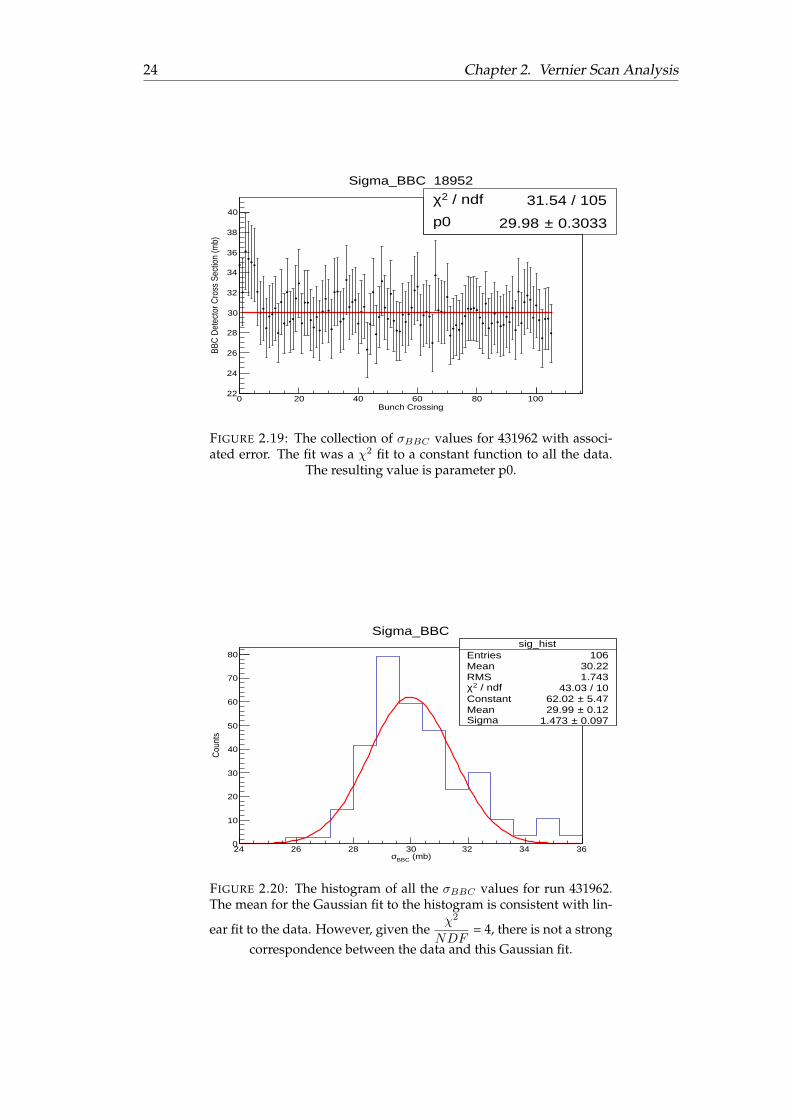
The results were consistent with previous years’ Vernier scans at PHENIX. How-ever, those previous years at PHENIX have shown that the value for σBBC can varyfrom run to run, more than the statistical variation within one run. This result willbe presented to the collaboration and a plan will be developed for how to best ac-count for this. Figure 2.19 below shows the values for σBBC as a function of bunchnumber, and figure 2.20 is a histogram of the same values.

It is important to notice in figure 2.19 there is a group of bunches near bunchcrossing 0 that are statistically higher than the remainder. These were included inthe final average, because the discrepancy was thought to be a result of the factthat β∗ and crossing angle corrections cannot be made on a bunch by bunch basis.Since the bunch near the beginning of the beam (approximately 0-7) are followingthe empty bunches (107-120) known as the abort gap, there is less of a space chargeeffect on the beginning bunches. This is a well understood effect, and is seen in otherVernier scans in past run years [5], and therefore it is not a concern.


Bunch Crossing0 20 40 60 80 100

BBC

Det

ecto

r Cro

ss S

ectio

n (m

b)

22

24

26

28

30

32

34

36

38

40 / ndf 2χ 31.54 / 105

p0 0.3033± 29.98

/ ndf 2χ 31.54 / 105

p0 0.3033± 29.98

Sigma_BBC 18952

FIGURE 2.19: The collection of σBBC values for 431962 with associ-ated error. The fit was a χ2 fit to a constant function to all the data.

The resulting value is parameter p0.

sig_histEntries 106Mean 30.22RMS 1.743

/ ndf 2χ 43.03 / 10Constant 5.47± 62.02 Mean 0.12± 29.99 Sigma 0.097± 1.473

(mb)BBCσ24 26 28 30 32 34 36

Cou

nts

0

10

20

30

40

50

60

70

80sig_hist

Entries 106Mean 30.22RMS 1.743

/ ndf 2χ 43.03 / 10Constant 5.47± 62.02 Mean 0.12± 29.99 Sigma 0.097± 1.473

Sigma_BBC

FIGURE 2.20: The histogram of all the σBBC values for run 431962.The mean for the Gaussian fit to the histogram is consistent with lin-

ear fit to the data. However, given theχ2

NDF= 4, there is not a strong

correspondence between the data and this Gaussian fit.

25

Appendix A

Bibliography

[1] W. Herr and B. Muratori. Concept of Luminosity. CERN Document Server.(2009).

[2] K. Adcox, et. al. PHENIX Detector Overview. Nuclear Instrumentation Meth-ods A, 469-479 (2003).

[3] M. Allen et al. PHENIX Inner Detector. Nuclear Instrumentation Methods A,521-536 (2003).

[4] C. Adler et al. The RHIC Zero Degree Calorimeters. Nuclear InstrumentationMethods A, (2001).

[5] A Drees. Analysis of Vernier Scans During RHIC Run-13. 13:1-18, Oct 2013.[6] A. Datta D. Kawall. Relative Luminosity Considerations. https://www.phenix.bnl.gov/WWW/pdraft/kawall/pwg/pwg

090304dmk.pdf, Mar 2009

Vernier Scan Analysis for PHENIX Run 15 p p+p...

Documents

Transcript of Vernier Scan Analysis for PHENIX Run 15 p p+p...