VeriML: A dependently-typed, user-extensible and …VeriML: A dependently-typed, user-extensible and...

Abstract

VeriML: A dependently-typed, user-extensible and language-centricapproach to proof assistants

Antonios Michael Stampoulis2013

Software certification is a promising approach to producing programs which are virtually free of bugs. It requires theconstruction of a formal proof which establishes that the code in question will behave according to its specification– a higher-level description of its functionality. The construction of such formal proofs is carried out in tools calledproof assistants. Advances in the current state-of-the-art proof assistants have enabled the certification of a numberof complex and realistic systems software.

Despite such success stories, large-scale proof development is an arcane art that requires significant manual effortand is extremely time-consuming. The widely accepted best practice for limiting this effort is to develop domain-specific automation procedures to handle all but the most essential steps of proofs. Yet this practice is rarely followedor needs comparable development effort as well. This is due to a profound architectural shortcoming of existingproof assistants: developing automation procedures is currently overly complicated and error-prone. It involves theuse of an amalgam of extension languages, each with a different programming model and a set of limitations, andwith significant interfacing problems between them.

This thesis posits that this situation can be significantly improved by designing a proof assistant with extensibil-ity as the central focus. Towards that effect, I have designed a novel programming language called VeriML, whichcombines the benefits of the different extension languages used in current proof assistants while eschewing theirlimitations. The key insight of the VeriML design is to combine a rich programming model with a rich type system,which retains at the level of types information about the proofs manipulated inside automation procedures. The ef-fort required for writing new automation procedures is significantly reduced by leveraging this typing informationaccordingly.

I show that generalizations of the traditional features of proof assistants are a direct consequence of the VeriMLdesign. Therefore the language itself can be seen as the proof assistant in its entirety and also as the single languagethe user has to master. Also, I show how traditional automation mechanisms offered by current proof assistantscan be programmed directly within the same language; users are thus free to extend them with domain-specificsophistication of arbitrary complexity.

In this dissertation I present all aspects of the VeriML language: the formal definition of the language; an ex-tensive study of its metatheoretic properties; the details of a complete prototype implementation; and a number ofexamples implemented and tested in the language.

VeriML: A dependently-typed, user-extensible and

language-centric approach to proof assistants

A DissertationPresented to the Faculty of the Graduate School

ofYale University

in Candidacy for the Degree ofDoctor of Philosophy

byAntonios Michael Stampoulis

Dissertation Director: Zhong Shao

May 2013

Copyright c© 2013 by Antonios Michael StampoulisAll rights reserved.

ii

Contents

List of Figures v

List of Tables viii

List of Code Listings ix

Acknowledgements xi

1 Introduction 11.1 Problem description . . . . . . . . . . . . . . . . . . . . . . . . . . . . . . . . . . . . . . . . . . . . . . . . . . . . . 21.2 Thesis statement . . . . . . . . . . . . . . . . . . . . . . . . . . . . . . . . . . . . . . . . . . . . . . . . . . . . . . . 41.3 Summary of results . . . . . . . . . . . . . . . . . . . . . . . . . . . . . . . . . . . . . . . . . . . . . . . . . . . . . 5

2 Informal overview 82.1 Proof assistant architecture . . . . . . . . . . . . . . . . . . . . . . . . . . . . . . . . . . . . . . . . . . . . . . . . 8

2.1.1 Preliminary notions . . . . . . . . . . . . . . . . . . . . . . . . . . . . . . . . . . . . . . . . . . . . . . . . 82.1.2 Variations . . . . . . . . . . . . . . . . . . . . . . . . . . . . . . . . . . . . . . . . . . . . . . . . . . . . . . 112.1.3 Issues . . . . . . . . . . . . . . . . . . . . . . . . . . . . . . . . . . . . . . . . . . . . . . . . . . . . . . . . . 18

2.2 A new architecture: VeriML . . . . . . . . . . . . . . . . . . . . . . . . . . . . . . . . . . . . . . . . . . . . . . . . 192.3 Brief overview of the language . . . . . . . . . . . . . . . . . . . . . . . . . . . . . . . . . . . . . . . . . . . . . . 23

3 The logic λHOL: Basic framework 353.1 The base λHOL logic . . . . . . . . . . . . . . . . . . . . . . . . . . . . . . . . . . . . . . . . . . . . . . . . . . . . 353.2 Adding equality . . . . . . . . . . . . . . . . . . . . . . . . . . . . . . . . . . . . . . . . . . . . . . . . . . . . . . . . 393.3 λHOL as a Pure Type System . . . . . . . . . . . . . . . . . . . . . . . . . . . . . . . . . . . . . . . . . . . . . . . 423.4 λHOL using hybrid deBruijn variables . . . . . . . . . . . . . . . . . . . . . . . . . . . . . . . . . . . . . . . . . 44

4 The logic λHOL: Extension variables 544.1 λHOL with metavariables . . . . . . . . . . . . . . . . . . . . . . . . . . . . . . . . . . . . . . . . . . . . . . . . . 544.2 λHOL with extension variables . . . . . . . . . . . . . . . . . . . . . . . . . . . . . . . . . . . . . . . . . . . . . 624.3 Constant schemata in signatures . . . . . . . . . . . . . . . . . . . . . . . . . . . . . . . . . . . . . . . . . . . . . 734.4 Named extension variables . . . . . . . . . . . . . . . . . . . . . . . . . . . . . . . . . . . . . . . . . . . . . . . . . 74

5 The logic λHOL: Pattern matching 775.1 Pattern matching . . . . . . . . . . . . . . . . . . . . . . . . . . . . . . . . . . . . . . . . . . . . . . . . . . . . . . . 775.2 Collapsing extension variables . . . . . . . . . . . . . . . . . . . . . . . . . . . . . . . . . . . . . . . . . . . . . . 105

iii

6 The VeriML computational language 1126.1 Base computation language . . . . . . . . . . . . . . . . . . . . . . . . . . . . . . . . . . . . . . . . . . . . . . . . 112

6.1.1 Presentation and formal definition . . . . . . . . . . . . . . . . . . . . . . . . . . . . . . . . . . . . . . 1126.1.2 Metatheory . . . . . . . . . . . . . . . . . . . . . . . . . . . . . . . . . . . . . . . . . . . . . . . . . . . . . 121

6.2 Derived pattern matching forms . . . . . . . . . . . . . . . . . . . . . . . . . . . . . . . . . . . . . . . . . . . . . 1286.3 Staging . . . . . . . . . . . . . . . . . . . . . . . . . . . . . . . . . . . . . . . . . . . . . . . . . . . . . . . . . . . . . . 1346.4 Proof erasure . . . . . . . . . . . . . . . . . . . . . . . . . . . . . . . . . . . . . . . . . . . . . . . . . . . . . . . . . 141

7 User-extensible static checking 1457.1 User-extensible static checking for proofs . . . . . . . . . . . . . . . . . . . . . . . . . . . . . . . . . . . . . . . 149

7.1.1 The extensible conversion rule . . . . . . . . . . . . . . . . . . . . . . . . . . . . . . . . . . . . . . . . . 1497.1.2 Proof object expressions as certificates . . . . . . . . . . . . . . . . . . . . . . . . . . . . . . . . . . . . 158

7.2 User-extensible static checking for tactics . . . . . . . . . . . . . . . . . . . . . . . . . . . . . . . . . . . . . . . 1607.3 Programming with dependently-typed data structures . . . . . . . . . . . . . . . . . . . . . . . . . . . . . . . 167

8 Prototype implementation 1768.1 Overview . . . . . . . . . . . . . . . . . . . . . . . . . . . . . . . . . . . . . . . . . . . . . . . . . . . . . . . . . . . . 1768.2 Logic implementation . . . . . . . . . . . . . . . . . . . . . . . . . . . . . . . . . . . . . . . . . . . . . . . . . . . . 178

8.2.1 Type inference for logical terms . . . . . . . . . . . . . . . . . . . . . . . . . . . . . . . . . . . . . . . . 1808.2.2 Inductive definitions . . . . . . . . . . . . . . . . . . . . . . . . . . . . . . . . . . . . . . . . . . . . . . . . 184

8.3 Computational language implementation . . . . . . . . . . . . . . . . . . . . . . . . . . . . . . . . . . . . . . . 1878.3.1 Surface syntax extensions . . . . . . . . . . . . . . . . . . . . . . . . . . . . . . . . . . . . . . . . . . . . 1888.3.2 Translation to OCaml . . . . . . . . . . . . . . . . . . . . . . . . . . . . . . . . . . . . . . . . . . . . . . 1928.3.3 Staging . . . . . . . . . . . . . . . . . . . . . . . . . . . . . . . . . . . . . . . . . . . . . . . . . . . . . . . . 1948.3.4 Proof erasure . . . . . . . . . . . . . . . . . . . . . . . . . . . . . . . . . . . . . . . . . . . . . . . . . . . . 1958.3.5 VeriML as a toplevel and VeriML as a translator . . . . . . . . . . . . . . . . . . . . . . . . . . . . . . 195

9 Examples and Evaluation 1979.1 Basic support code . . . . . . . . . . . . . . . . . . . . . . . . . . . . . . . . . . . . . . . . . . . . . . . . . . . . . . 1979.2 Extensible rewriters . . . . . . . . . . . . . . . . . . . . . . . . . . . . . . . . . . . . . . . . . . . . . . . . . . . . . 2009.3 Naive equality rewriting . . . . . . . . . . . . . . . . . . . . . . . . . . . . . . . . . . . . . . . . . . . . . . . . . . 2059.4 Equality with uninterpreted functions . . . . . . . . . . . . . . . . . . . . . . . . . . . . . . . . . . . . . . . . . 2059.5 Automated proof search for first-order formulas . . . . . . . . . . . . . . . . . . . . . . . . . . . . . . . . . . . 2129.6 Natural numbers . . . . . . . . . . . . . . . . . . . . . . . . . . . . . . . . . . . . . . . . . . . . . . . . . . . . . . . 2159.7 Normalizing natural number expressions . . . . . . . . . . . . . . . . . . . . . . . . . . . . . . . . . . . . . . . 2209.8 Evaluation . . . . . . . . . . . . . . . . . . . . . . . . . . . . . . . . . . . . . . . . . . . . . . . . . . . . . . . . . . . 224

10 Related work 22710.1 Development of tactics and proof automation . . . . . . . . . . . . . . . . . . . . . . . . . . . . . . . . . . . . 22710.2 Proof assistant architecture . . . . . . . . . . . . . . . . . . . . . . . . . . . . . . . . . . . . . . . . . . . . . . . . 23310.3 Extensibility of the conversion rule . . . . . . . . . . . . . . . . . . . . . . . . . . . . . . . . . . . . . . . . . . . 23410.4 Type-safe manipulation of languages with binding . . . . . . . . . . . . . . . . . . . . . . . . . . . . . . . . . 23510.5 Mixing logic with computation . . . . . . . . . . . . . . . . . . . . . . . . . . . . . . . . . . . . . . . . . . . . . . 236

11 Conclusion and future work 238

iv

Bibliography 244

v

List of Figures

2.1 Basic architecture of proof assistants . . . . . . . . . . . . . . . . . . . . . . . . . . . . . . . . . . . . . . . . . . 92.2 Programming languages available for writing automation procedures in the Coq architecture . . . . . 152.3 Comparison of architecture between current proof assistants and VeriML . . . . . . . . . . . . . . . . . 192.4 Comparison of small-scale automation approach between current proof assistants and VeriML . . . . 21

3.1 The base syntax of the logic λHOL . . . . . . . . . . . . . . . . . . . . . . . . . . . . . . . . . . . . . . . . . . . 363.2 The typing rules of the logic λHOL . . . . . . . . . . . . . . . . . . . . . . . . . . . . . . . . . . . . . . . . . . 363.3 The typing rules of the logic λHOL (continued) . . . . . . . . . . . . . . . . . . . . . . . . . . . . . . . . . . 373.4 Capture avoiding substitution . . . . . . . . . . . . . . . . . . . . . . . . . . . . . . . . . . . . . . . . . . . . . . . 373.5 The logic λHOLE : syntax and typing extensions for equality . . . . . . . . . . . . . . . . . . . . . . . . . . 413.6 The syntax of the logic λHOL given as a PTS . . . . . . . . . . . . . . . . . . . . . . . . . . . . . . . . . . . . 423.7 The typing rules of the logic λHOL in PTS style . . . . . . . . . . . . . . . . . . . . . . . . . . . . . . . . . . 433.8 The logic λHOL with hybrid deBruijn variable representation: Syntax . . . . . . . . . . . . . . . . . . . . 463.9 The logic λHOL with hybrid deBruijn variable representation: Typing Judgements . . . . . . . . . . . 473.10 The logic λHOL with hybrid deBruijn variable representation: Typing Judgements (continued) . . . 473.11 The logic λHOL with hybrid deBruijn variable representation: Freshening and Binding . . . . . . . . 483.12 The logic λHOL with hybrid deBruijn variable representation: Variable limits . . . . . . . . . . . . . . . 493.13 The logic λHOL with hybrid deBruijn variable representation: Substitution Application and Iden-

tity Substitution . . . . . . . . . . . . . . . . . . . . . . . . . . . . . . . . . . . . . . . . . . . . . . . . . . . . . . . 49

4.1 Extension of λHOL with meta-variables: Syntax and Syntactic Operations . . . . . . . . . . . . . . . . . 554.2 Extension of λHOL with meta-variables: Typing rules . . . . . . . . . . . . . . . . . . . . . . . . . . . . . . 564.3 Extension of λHOL with meta-variables: Meta-substitution application . . . . . . . . . . . . . . . . . . . 574.4 Extension of λHOL with parametric contexts: Syntax . . . . . . . . . . . . . . . . . . . . . . . . . . . . . . 644.5 Extension of λHOL with parametric contexts: Syntactic Operations (Length and access of substitu-

tions and contexts; Substitution application; Identity substitution and partial identity substitution) . 644.6 Extension of λHOL with parametric contexts: Variable limits . . . . . . . . . . . . . . . . . . . . . . . . . 654.7 Extension of λHOL with parametric contexts: Syntactic Operations (Freshening and binding) . . . . 654.8 Extension of λHOL with parametric contexts: Subsumption . . . . . . . . . . . . . . . . . . . . . . . . . . 654.9 Extension of λHOL with parametric contexts: Typing . . . . . . . . . . . . . . . . . . . . . . . . . . . . . . 664.10 Extension of λHOL with parametric contexts: Typing (continued) . . . . . . . . . . . . . . . . . . . . . . 664.11 Extension of λHOL with parametric contexts: Extension substitution application . . . . . . . . . . . . 674.12 Extension to λHOL with constant-schema-based signatures: Syntax and typing . . . . . . . . . . . . . . 744.13 Definition of polymorphic lists in λHOL through constant schemata . . . . . . . . . . . . . . . . . . . . . 75

vi

4.14 λHOL with named extension variables: Syntax . . . . . . . . . . . . . . . . . . . . . . . . . . . . . . . . . . . 754.15 λHOL with named extension variables: Typing . . . . . . . . . . . . . . . . . . . . . . . . . . . . . . . . . . . 76

5.1 Pattern typing for λHOL . . . . . . . . . . . . . . . . . . . . . . . . . . . . . . . . . . . . . . . . . . . . . . . . . 805.2 Pattern typing for λHOL (continued) . . . . . . . . . . . . . . . . . . . . . . . . . . . . . . . . . . . . . . . . . 815.3 Syntactic operations for unification contexts . . . . . . . . . . . . . . . . . . . . . . . . . . . . . . . . . . . . . 825.4 Partial contexts (syntax and typing) . . . . . . . . . . . . . . . . . . . . . . . . . . . . . . . . . . . . . . . . . . . 855.5 Partial contexts (syntactic operations) . . . . . . . . . . . . . . . . . . . . . . . . . . . . . . . . . . . . . . . . . 855.6 Relevant variables of λHOL derivations . . . . . . . . . . . . . . . . . . . . . . . . . . . . . . . . . . . . . . . . 865.7 Relevant variables of λHOL derivations (continued) . . . . . . . . . . . . . . . . . . . . . . . . . . . . . . . . 875.8 Partial substitutions (syntax and typing) . . . . . . . . . . . . . . . . . . . . . . . . . . . . . . . . . . . . . . . . 915.9 Partial substitutions (syntactic operations) . . . . . . . . . . . . . . . . . . . . . . . . . . . . . . . . . . . . . . 925.10 Pattern matching algorithm for λHOL, operating on derivations (1/3) . . . . . . . . . . . . . . . . . . . . 925.11 Pattern matching algorithm for λHOL, operating on derivations (2/3) . . . . . . . . . . . . . . . . . . . . 935.12 Pattern matching algorithm for λHOL, operating on derivations (3/3) . . . . . . . . . . . . . . . . . . . . 935.13 Annotated λHOL terms (syntax) . . . . . . . . . . . . . . . . . . . . . . . . . . . . . . . . . . . . . . . . . . . . 1015.14 Pattern matching algorithm for λHOL, operating on annotated terms . . . . . . . . . . . . . . . . . . . . 1025.15 Conversion of typing derivations to annotated terms . . . . . . . . . . . . . . . . . . . . . . . . . . . . . . . 1035.16 Operation to decide whether λHOL terms are collapsable with respect to the extension context . . . 1065.17 Operation to decide whether λHOL terms are collapsable with respect to the extension context

(continued) . . . . . . . . . . . . . . . . . . . . . . . . . . . . . . . . . . . . . . . . . . . . . . . . . . . . . . . . . . . 107

6.1 VeriML computational language: ML core (syntax) . . . . . . . . . . . . . . . . . . . . . . . . . . . . . . . . . 1136.2 VeriML computational language: λHOL-related constructs (syntax) . . . . . . . . . . . . . . . . . . . . . . 1136.3 VeriML computational language: ML core (typing, 1/3) . . . . . . . . . . . . . . . . . . . . . . . . . . . . . . 1146.4 VeriML computational language: ML core (typing, 2/3) . . . . . . . . . . . . . . . . . . . . . . . . . . . . . . 1156.5 VeriML computational language: ML core (typing, 3/3) . . . . . . . . . . . . . . . . . . . . . . . . . . . . . . 1156.6 VeriML computational language: λHOL-related constructs (typing) . . . . . . . . . . . . . . . . . . . . . . 1166.7 VeriML computational language: λHOL-related constructs (typing, continued) . . . . . . . . . . . . . . 1166.8 VeriML computational language: ML core (semantics) . . . . . . . . . . . . . . . . . . . . . . . . . . . . . . . 1176.9 VeriML computational language: λHOL-related constructs (semantics) . . . . . . . . . . . . . . . . . . . . 1176.10 VeriML computational language: definitions used in metatheory . . . . . . . . . . . . . . . . . . . . . . . . 1226.11 Derived VeriML pattern matching constructs: Multiple branches . . . . . . . . . . . . . . . . . . . . . . . 1296.12 Derived VeriML pattern matching constructs: Environment-refining matching . . . . . . . . . . . . . . 1316.13 Derived VeriML pattern matching constructs: Simultaneous matching . . . . . . . . . . . . . . . . . . . . 1336.14 VeriML computational language: Staging extension (syntax) . . . . . . . . . . . . . . . . . . . . . . . . . . . 1366.15 VeriML computational language: Staging extension (typing) . . . . . . . . . . . . . . . . . . . . . . . . . . . 1366.16 VeriML computational language: Staging extension (operational semantics) . . . . . . . . . . . . . . . . . 1376.17 Proof erasure for VeriML . . . . . . . . . . . . . . . . . . . . . . . . . . . . . . . . . . . . . . . . . . . . . . . . . . 1426.18 Proof erasure: Adding the prove-anything constant to λHOL . . . . . . . . . . . . . . . . . . . . . . . . . . 143

7.1 Layers of static checking and steps in the corresponding formal proof of even (twice x) . . . . . . . . . . 1467.2 User-extensible static checking of tactics . . . . . . . . . . . . . . . . . . . . . . . . . . . . . . . . . . . . . . . . 1487.3 The logic λHOLC : Adding the conversion rule to the λHOL logic . . . . . . . . . . . . . . . . . . . . . . 150

vii

7.4 Conversion of λHOLC proof objects into VeriML proof object expressions . . . . . . . . . . . . . . . . . 155

8.1 Components of the VeriML implementation . . . . . . . . . . . . . . . . . . . . . . . . . . . . . . . . . . . . . 1778.2 Extension to λHOL signatures with definitions: Syntax and typing . . . . . . . . . . . . . . . . . . . . . . 1798.3 Extension λHOL with positivity types . . . . . . . . . . . . . . . . . . . . . . . . . . . . . . . . . . . . . . . . . 186

viii

List of Tables

3.1 Comparison of variable representation techniques . . . . . . . . . . . . . . . . . . . . . . . . . . . . . . . . . 46

8.1 Concrete syntax for λHOL terms . . . . . . . . . . . . . . . . . . . . . . . . . . . . . . . . . . . . . . . . . . . . 1798.2 Translation of λHOL-related VeriML constructs to simply-typed OCaml constructs . . . . . . . . . . . 192

9.1 Line counts for code implemented in VeriML . . . . . . . . . . . . . . . . . . . . . . . . . . . . . . . . . . . . 2259.2 Comparison of line counts for EUF rewriting and arithmetic simplification between VeriML and Coq225

ix

List of Code Listings

7.1 Implementation of the definitional equality checker in VeriML (1/2) . . . . . . . . . . . . . . . . . . . . . 1537.2 Implementation of the definitional equality checker in VeriML (2/2) . . . . . . . . . . . . . . . . . . . . . 1547.3 VeriML rewriter that simplifies uses of the natural number addition function in logical terms . . . . . 1617.4 VeriML rewriter that simplifies uses of the natural number addition function in logical terms, with

proof obligations filled-in . . . . . . . . . . . . . . . . . . . . . . . . . . . . . . . . . . . . . . . . . . . . . . . . . 1647.5 Version of vector append with explicit proofs . . . . . . . . . . . . . . . . . . . . . . . . . . . . . . . . . . . . 1709.1 Definition of basic datatypes and associated functions . . . . . . . . . . . . . . . . . . . . . . . . . . . . . . . 1989.2 Examples of proof object constructors lifted into VeriML tactics . . . . . . . . . . . . . . . . . . . . . . . . 1999.3 Building a rewriter from a list of rewriter modules . . . . . . . . . . . . . . . . . . . . . . . . . . . . . . . . . 2019.4 Global registering of rewriter modules . . . . . . . . . . . . . . . . . . . . . . . . . . . . . . . . . . . . . . . . . 2029.5 Basic equality checkers: syntactic equality and compatible closure . . . . . . . . . . . . . . . . . . . . . . . 2039.6 Global registration of equality checkers and default equality checking . . . . . . . . . . . . . . . . . . . . . 2049.7 Naive rewriting for equality hypotheses . . . . . . . . . . . . . . . . . . . . . . . . . . . . . . . . . . . . . . . . 2069.8 Implementation of hash table with dependent key-value pairs and of sets of terms as pairs of a

hashtable and a list . . . . . . . . . . . . . . . . . . . . . . . . . . . . . . . . . . . . . . . . . . . . . . . . . . . . . . 2089.9 find – Finding the equivalence class representative of a term . . . . . . . . . . . . . . . . . . . . . . . . . . 2099.10 union – Merging equivalence classes . . . . . . . . . . . . . . . . . . . . . . . . . . . . . . . . . . . . . . . . . . 2109.11 simple_eq, congruent_eq – Checking equality based on existing knowledge . . . . . . . . . . . . . . . 2109.12 merge – Incorporating a new equality hypothesis . . . . . . . . . . . . . . . . . . . . . . . . . . . . . . . . . . 2119.13 equalchecker_euf – Equality checking module for EUF theory . . . . . . . . . . . . . . . . . . . . . . . 2119.14 Rewriter module for β-reduction . . . . . . . . . . . . . . . . . . . . . . . . . . . . . . . . . . . . . . . . . . . . 2129.15 autoprove – Main function for automated proving of first-order formulas . . . . . . . . . . . . . . . . . 2139.16 findhyp – Search for a proof of a goal in the current hypotheses . . . . . . . . . . . . . . . . . . . . . . . . 2149.17 autoprove_with_hyp – Auxiliary function for proving a goal assuming an extra hypothesis . . . . . 2159.18 Definition of natural numbers and natural induction tactic . . . . . . . . . . . . . . . . . . . . . . . . . . . . 2169.19 Addition for natural numbers . . . . . . . . . . . . . . . . . . . . . . . . . . . . . . . . . . . . . . . . . . . . . . . 2189.20 Multiplication for natural numbers . . . . . . . . . . . . . . . . . . . . . . . . . . . . . . . . . . . . . . . . . . . 2199.21 Definition of lists and permutations in λHOL, with associated theorems . . . . . . . . . . . . . . . . . . 2219.22 Selection sorting for lists . . . . . . . . . . . . . . . . . . . . . . . . . . . . . . . . . . . . . . . . . . . . . . . . . . 2229.23 Rewriter module for arithmetic simplification (1/2) . . . . . . . . . . . . . . . . . . . . . . . . . . . . . . . . 2239.24 Rewriter module for arithmetic simplification (2/2) . . . . . . . . . . . . . . . . . . . . . . . . . . . . . . . . 224

x

Acknowledgements

This dissertation would have been impossible without the help, advice and support of a great number of people.They all have my deepest gratitude.

First of all, I would like to thank my advisor, Zhong Shao, for giving me the chance to work on an excit-ing research topic, for his constant help and his input on this work and for supporting me in every way possiblethroughout these years. His insights and close supervision were of critical importance in the first stages of thisresearch; his eye for intellectual clarity and simplicity were tremendously influential in the later stages of the devel-opment of the VeriML theory and implementation. He gave me the space to work out things on my own whenI needed it and when I wanted to concentrate on the development of VeriML, yet he was always available when Ineeded his opinion. I am indebted to him for all of his advice and suggestions, for being patient with me and forinstilling the true qualities of a researcher in me. I am leaving Yale with fond memories of our endless discussionsin his office; I hope these will continue in the years to follow.

I would also like to express my gratitude to the rest of my committee, Paul Hudak, Drew McDermott and XavierLeroy, for their advice during these years and for taking the time to read this dissertation. They have all influencedthis work, Paul through his research and his profound, insightful lectures on Haskell and formal semantics; Drew byhis suggestion to look at resolution-based provers, starting a path which eventually led to reading and implementingthe equality with uninterpreted functions procedure; and Xavier by showing that software certification is possibleand exciting through the development of CompCert, by creating OCaml which was a pleasure to use in order todevelop VeriML, and by his excitement and encouragement when I first asked him to serve in my committee anddescribed the VeriML idea to him.

I would also like to thank the rest of my professors at Yale, especially Bryan Ford, Richard Yang, Gaja Jarosz,Yiorgos Makris and Andreas Savvides. Nikolaos Papaspyrou, my undegraduate thesis advisor, has influenced megreatly through his supervision at NTUA; my initial interest in programming languages research in general anddependent types in particular is due to him. Ella Bounimova gave me the chance to work at Microsoft ResearchRedmond as a summer intern during my first year at Yale; I am grateful to her as well as Tom Ball and Vlad Levin,my two other mentors at Microsoft at the time.

During my time at Yale, I have had the pleasure to collaborate and discuss research and non-research with manycolleagues. I would especially like to thank Andi Voellmy, my office-mate, for our discussions and his input dur-ing the six years of our Ph.D.; all the past, present and newly-arrived members of the FLINT group, especiallyXinyu Feng, Alex Vaynberg, Rodrigo Ferreira, David Costanzo, Shu-Chun Weng, Jan Hoffmann and Mike Mar-mar. Zhong Zhuang deserves special mention for using the VeriML prototype for his own research. I would alsolike to thank the rest of my friends in the CS department, especially Nikhil, Eli, Amittai, Dan, Edo, Lev, Aaron,Pradipta and Justin. A number of researchers and colleagues whom I have discussed this work with in conferencesand beyond have also been profoundly influential; I would like to especially thank Herman Geuvers, Brigitte Pien-tka, Carsten Schürmann, Andreas Abel, Randy Pollack, Adam Chlipala, Viktor Vafeiadis, Dimitrios Vytiniotis,

xi

Christos Dimoulas, Daniel Licata and Gregory Malecha.This work was supported in part by the NSF grants CCF-0811665, CNS-0915888, CNS-0910670 and CNS-

1065451 and by the DARPA CRASH grant FA8750-10-2-0254. I would like to thank both agencies, as well as YaleUniversity and the Department of Computer Science, for supporting me during these years and making this workpossible.

During my time in New Haven I was extremely lucky to meet many amazing people that made my Ph.D. yearsunforgettable. Argyro and Mihalis have been next to me in the most fun and happy moments and in the hardesttimes as well; they have been infinitely patient with me and very supportive. During these years they became mysecond family and I thank them a lot. I would also like to thank Dimitris ‘the Teacher’ and Maria, for showingme the ropes in my first year; my roomie Thanassis for his friendship and patience, for our time in Mansfield St.as well as for his excellent cooking; Maria for our endless walks and talks in the HGS courtyard; Marisa and theZattas brothers, especially for being around during this last year; Kostas, for his friendship and his generosity –offering me a place to stay during the last months of my Ph.D.; Petros, Tasos, Nikos, Roula, Yiorgos and theirwonderful daughter Zoi, Palmyra, Sotiria and the rest of the Greeks at Yale. The members of the legendary SixthFlour Lounge: my roomates Dominik and Eugene, Yao, Isaak, Nana, Philip; also all my other friends during mytime in HGS, especially Yan and Serdar. The graphics and the organics for our times in New York, New Havenand Boston: Yiannis, Kostas, Rimi, Dan and Cagil – and Nikoletta, even though technically she was in Europe.Elli, for the fun times in Brooklyn and for her profound words and support; and the Yiorgides as well. The band:Randy (especially for convincing me to join again), Tarek, Cecily, Tomas, Anne, Ragy and Lucas. All of my otherfriends who supported me throughout these years, especially Areti, Danai, Ioanna, Themis, Enrico, Yiannis, Mairi,Alvertos, Melina and Panagiotis.

I am deeply grateful to all of my family for their love and their unwavering support in this long process. Myfather instilled in me his love of education and my mother her sense of perserverance, both of which were absolutelyessential for completing this work. I would like to thank my siblings Nikos and Eva for always believing in me;my siblings-in-law Chin Szu and Thodoris and my three adorable nieces who were born during my Ph.D., Natalie,Matina and Eirini; my uncles, aunts and cousins, especially uncle Thanos and cousin Antonis for the kind words ofsupport they offered and their appreciation of the hard work that goes into a doctoral dissertation.

Last, I would like to thank Erato, for being next to me during the good moments and the bad moments of thisPh.D., for her wisdom and advice, and for her constant love and support.

xii

Chapter 1

Introduction

Computer software is ubiquitous in our society. The repercussions of software errors are becoming increasinglymore severe, leading to huge financial losses every year [e.g. Zhivich and Cunningham, 2009] and even resulting inthe loss of human lives [e.g. Blair et al., 1992, Lions et al., 1996]. A promising research direction towards more robustsoftware is the idea of certified software [Shao, 2010]: software that comes together with a high-level description of itsbehavior – its specification. The software itself is related to its specification through an unforgeable formal proof thatincludes all possible details, down to some basic mathematical axioms. Recent success stories in this field include thecertified optimizing C compiler [Leroy, 2009] and the certified operating system kernel seL4 [Klein et al., 2009].

The benefit of formal proofs is that they can be mechanically checked for validity using a small computer pro-gram, owing to the high level of detail that they include. Their drawback is that they are hard to write, even when weutilize proof assistants – specialized tools that are designed to help in formal proof development. We argue that thisis due to a profound architectural shortcoming of current proof assistants: though extending a proof assistant withdomain-specific sophistication is of paramount importance for large-scale proof development [e.g. Chlipala et al.,2009, Morrisett et al., 2012], developing such extensions (in the form of proof-producing procedures) is currentlyoverly complex and error-prone.

This dissertation is an attempt to address this shortcoming of formal proof development in current systems.Towards that end, I have designed and developed a new programming language called VeriML, which serves as anovel proof assistant. The main benefit of VeriML is that it includes a rich type system which provides helpfulinformation and robustness guarantees when developing new proof-producing procedures for specialized domains.Furthermore, users can register such procedures to be utilized transparently by the proof assistant, so that thedevelopment of proofs and further procedures can be significantly simplified. Though an increasing number oftrivial details can be omitted in this way from proofs and proof procedures, the type system ensures that this doesnot eschew logical soundness – the resulting proofs are as trustworthy as formal proofs with full details. This leadsto a truly extensible proof assistant where domain-specific sophistication can be built up in layers.

1.1 Problem description

Formal proof development is a complicated endeavor. Formal proofs need to contain all possible details, downto some basic logical axioms. Contrast this with the informal proofs of normal mathematical practice: one needsto only point out the essential steps of the argument at hand. The person reading the proof needs to convincethemselves that these steps are sufficient and valid, relying on their intuition or even manually reconstructing some

1

missing parts of the proof (e.g. when the proof mentions that a certain statement is trivial, or that ‘other cases followsimilarly’). This is only possible if they are sufficiently familiar with the specific domain of the proof. Thus thedistinguishing characteristic is that the receiver of an informal proof is expected to possess certain sophistication,whereas the receiver of formal proof is an absolutely skeptical agent that only knows of certain basic reasoningprinciples.

Proof assistants are environments that provide users with mechanisms for formal proof development, whichbring this process closer to writing down an informal proof. One such mechanism is tactics: functions that produceproofs under certain circumstances. Alluding to a tactic is similar to suggesting a methodology in informal practice,such as ‘use induction on x’. Tactics range from very simple, corresponding to basic reasoning principles, to verysophisticated, corresponding to automated proof discovery for large classes of problems.

When working on a large proof development, users are faced with the choice of either using the already existingtactics to write their proofs, or to develop their own domain-specific tactics. The latter choice is often suggested asadvantageous [e.g. Morrisett et al., 2012], as it leads to more concise proofs that omit details, which are also morerobust to changes in the specifications – similar to informal proofs that expect a certain level of domain sophistica-tion on the part of the reader. But developing new tactics comes with its own set of problems, as tactics in currentproof assistants are hard to write. The reason is that the workflow that modern proof assistants have been designedto optimize is developing new proofs, not developing new tactics. For example, when a partial proof is given, theproof assistant informs the user about what remains to be proved; thus proofs are usually developed in an interactivedialog with the proof assistant. Similar support is not available for tactics and would be impossible to support usingcurrent tactic development languages. Tactics do not specify under which circumstances they are supposed to work,the type of arguments they expect, what proofs they are supposed to produce and whether the proofs they produceare actually valid. Formally, we say that tactic programming is untyped. This hurts composability of tactics and alsoallows a large potential for bugs that occur only on particular invocations of tactics. This lack of information is alsowhat makes interactive development of tactics impossible.

Other than tactics, proof assistants also provide mechanisms that are used implicitly and ubiquitously through-out the proof. These aim to handle trivial details that are purely artifacts of the high level of rigor needed in a formalproof, but would not be mentioned in an informal proof. Examples are the conversion rule, which automates purelycomputational arguments (e.g. determining that 5! = 120), and unification algorithms, which aim to infer detailsof the terms used in a proof that can be easily determined from the context (e.g. determining that the generic ad-dition symbol + refers to natural number addition when used as 5+ x). The mechanism of the conversion ruleis even integrated with the base proof checker, in order to keep formal proofs feasible in terms of size. We referto these mechanisms as small-scale automation in order to differentiate them from large-scale automation which isoffered by explicit reference to specific automation tactics and development of further ones, following Asperti andSacerdoti Coen [2010].

Small-scale automation mechanisms usually provide their own ways for adding domain-specific extensions tothem; this allows users to provide transparent automation for the trivial details of the domain at hand. For exam-ple, unification mechanisms can be extended through first-order lemmas; and the conversion rule can support thedevelopment of automation procedures that are correct by construction. Still, the programming model that is sup-ported for these extensions is inherrently quite limited. In the case of the conversion rule this is because of its tightcoupling with the core of the proof assistant; in the case of unification, this because of the very way the automationmechanism work. On the other hand, the main cost in developing such extensions is in proving associated lemmas;therefore it significantly benefits from the main workflow of current proof assistants for writing proofs.

Contrasting this distinction between small-scale and large-scale automation with the practice of informal proof

2

reveals a key insight: the distinction between what constitutes a trivial detail that is best left implicit and whatconstitutes an essential detail of a proof is very thin; and it is arbitrary at best. Furthermore, as we progress towardsmore complex proofs in a certain domain, or from one domain A to a more complicated one B, which presupposesdomain A (e.g. algebra and calculus), it is crucial to omit more details. Therefore, the fact that small-scale automa-tion and large-scale automation are offered through very different means is a liability in as far as it precludes movingautomation from one side to the other. Users can develop the exact automation algorithms they have in mind as alarge-scale automation tactic; but there is significant re-engineering required if they want this to become part of the‘background reasoning’ offered by the small-scale automation mechanisms. They will have to completely rewritethose algorithms and even change the data structures they use, in order to match the limitations of the programmingmodel for small-scale automation. In cases where such limitations would make the algorithms suboptimal, the onlyalternative is to extend the very implementation of the small-scale automation mechanisms in the internals of theproof assistant. While this has been attempted in the past, it is obviously associated with a large development costand raises the question whether the overall system is still logically sound.

Overall, users are faced with a choice between multiple mechanisms when trying to develop automation for anew domain. Each mechanism has its own programming model and a set of benefits, issues and limitations. In manycases, users have to be proficient in multiple of these mechanisms in order to achieve the desired result in terms ofverbosity in the resulting proof, development cost, robustness and efficiency. The fact that significant issues exist ininterfacing between the various mechanisms and languages involved, further limits the extensibility and reusabilityof the automation that users develop.

In this dissertation, we propose a novel architecture for proof assistants, guided from the following insights.First, development of proof-producing procedures such as tactics should be a central focal point for proof assistants,just as development of proofs is of central importance in current proof assistants. Second, the distinction betweenlarge-scale automation and small-scale automation should be de-emphasized in light of their similarities: the involvedmechanisms are in essence proof-producing procedures, which work under certain circumstances and leverage dif-ferent algorithms. Third, that writing such proof-producing procedures in a single general-purpose programmingmodel coupled with a rich type system, directly offers the benefits of the traditional proof assistant architecture andgeneralizes them.

Based on these insights, we present a novel language-based architecture for proof assistants. We propose a new pro-gramming language, called VeriML, which focuses on the development of typed proof-producing procedures. Proofs,as well as other logic-related terms such as propositions, are explicitly represented and manipulated in the language;their types precisely capture the relationships between such terms (e.g. a proof which proves a specific proposi-tion). We show how this language enables us to support the traditional workflows of developing proofs and tacticsin current proof assistants, utilizing the information present in the type system to recover and extend the benefitsassociated with these workflows. We also show that small-scale automation mechanisms can be implemented withinthe language, rather than be hardcoded within its internal implementation. We demonstrate this fact through animplementation of the conversion rule within the language; we show how it can be made to behave identically to ahardcoded conversion rule. In this way we solve the long-standing problem of enabling arbitrary user extensions toconversion while maintaining logical soundness, by leveraging the rich type system of the language. Last, we showthat once domain-specific automation is developed it can transparently benefit the development of not only proofs,but further tactics and automation procedures as well. Overall, this results in a style of formal proof that comes onestep closer to informal proof, by increasing the potential for omitting details, while maintaining the same guaranteeswith respect to logical soundness.

3

1.2 Thesis statement

The thesis statement that this dissertation establishes follows.

A type-safe programming language combining typed manipulation of logical terms with a general-purpose side-effectful programming model is theoretically possible, practically implementable, viable asan alternative architecture for a proof assistant and offers improvements over the current proof assistantarchitectures.

By ‘logical terms’ we refer to the terms of a specific higher-order logic, such as propositions and proofs. Thelogic that we use is called λHOL and is specified as a type system in Chapter 3. By ‘manipulation’ we mean theability to introduce logical terms, pass them as arguments to functions, emit them as results from functions andalso pattern match on their structure programmatically. By ‘typed manipulation’ we mean that the logical-leveltyping information of logical terms is retained during such manipulation. By ‘type-safe’ we mean that subjectreduction holds for the programming language. By ‘general-purpose side-effectful programming model’ we mean aprogramming model that includes at the very least datatypes, general recursion and mutable references. We choosethe core ML calculus to satisfy this requirement. We demonstrate theoretical possibility by designing a type systemand operational semantics for this programming language and establishing its metatheory. We demonstrate practicalimplementability through an extensive prototype implementation of the language, which is sufficiently efficient inorder to test various examples in the language. We demonstrate viability as a proof assistant by implementing a setof examples tactics and proofs in the language. We demonstrate the fact that this language offers improvements overcurrent proof assistant architectures by showing that it enables user-extensible static checking of proofs and tacticsand utilizing such support in our examples. We demonstrate how this support simplifies complex implementationsof similar examples in traditional proof assistants.

1.3 Summary of results

In this section I present the technical results of my dissertation research.

1. Formal design of VeriML. I have developed a type system and operational semantics supporting a combina-tion of general-purpose, side-effectful programming with first-class typed support for logical term manipula-tion. The support for logical terms allows specifying the input-output behavior of functions that manipulatelogical terms. The language includes support for pattern matching over open logical terms, as well as overvariable environments. The type system works by leveraging contextual type theory for representing openlogical terms as well as the variable environments they depend on. I also show a number of extensions to thecore language, such as a simple staging construct and a proof erasure procedure.

2. Metatheory. I have proved a number of metatheoretic results for the above language.

Type safety ensures that a well-typed expression of the language evaluates to a well-typed value of the sametype, in the case where evaluation is successful and terminates. This is crucial in ensuring that the typethat is statically assigned to an expression can be trusted. For example, it follows that expressions whosestatic type claims that a proof for a specific proposition will be created indeed produce such a proof uponsuccessful evaluation.

Type safety for static evaluation ensures that the extension of the language with the staging construct forstatic evaluation of expressions obeys the same safety principle.

4

Compatibility of normal and proof-erasure semantics establishes that every step in the evaluation of asource expression that has all proof objects erased corresponds to a step in the evaluation of the originalsource expression. This guarantees that even if we choose not to generate proof objects while evaluatingexpressions of the language, valid proof objects of the right type always exist. Thus, if users are willingto trust the type checker and runtime system of VeriML, they can use the optimized semantics whereno proof objects get created.

Collapsing transformation of contextual terms establishes that under reasonable limitations with respectto the definition and use of contextual variables, a contextual term can be transformed into one that doesnot mention such contextual variables. This proof provides a way to transform proof expressions insidetactics into static proof expressions evaluated statically, at the time that the tactic is defined, using staging.

3. Prototype implementation. I have developed a prototype implementation of VeriML in OCaml, which isused to type check and evaluate a wide range of examples. The prototype has an extensive feature set over thepure language as described formally, supporting type inference, surface syntax for logical terms and VeriMLcode, special tactic syntax and translation to simply-typed OCaml code.

4. Extensible conversion rule. We showcase how VeriML can be used to solve the long-standing problem of auser-extensible conversion rule. The conversion rule that we describe combines the following characteristics: itis safe, meaning that it preserves logical soundness; it is user-extensible, using a familiar, generic programmingmodel; and, it does not require metatheoretic additions to the logic, but can be used to simplify the logicinstead. Also, we show how this conversion rule enables receivers of a formal proof to choose the exact sizeof the trusted core of formal proof checking; this choice is traditionally only available at the time that a logicis designed. We believe this is the first technique that combines these characteristics leading to a safe anduser-extensible static checking technique for proofs.

5. Static proof expressions. I describe a method that enables discovery and proof of required lemmas withintactics. This method requires minimal programmer annotation and increases the static guarantees provided bythe tactics, by removing potential sources of errors. I showcase how the same method can be used to separatethe proof-related aspect of writing a new tactic from the programming-related aspect, leading to increasedseparation of concerns.

6. Dependently typed programming. I also show how static proof expressions can be useful in traditionaldependently-typed programming (in the style of Dependent ML [Xi and Pfenning, 1999] and Agda [Norell,2007]), exactly because of the increased separation of concerns between the programming and the proof-related aspects. By combining this with the support for writing automation tactics within VeriML, we showhow our language enables a style of dependently-typed programming where the extra proof obligations aregenerated and resolved within the same language.

7. Technical advances in metatheoretic techniques. The metatheory for VeriML that I have developed in-cludes a number of technical advances over developments for similar languages such as Delphin or Beluga.These are:

– Orthogonality between logic and computation. The theorems that we prove about the computationallanguage do not depend on specifics of the logic language, save for a number of standard theorems aboutit. These theorems establish certain substitution and weakening lemmas for the logic language, as wellas the existence of an effective pattern matching procedure for terms of this language. This makes the

5

metatheory of the computational language modular with respect to the logic language, enabling us toextend or even replace the logic language in the future.

– Hybrid deBruijn variable representation. We use a concrete variable representation for variables of thelogic language instead of using the named approach for variables. This elucidates the definitions of thevarious substitution forms, especially wih respect to substitution of a polymorphic context with a con-crete one; it also makes for precise substitution lemma statements. It is also an efficient implementationtechnique for variables and enables subtyping based on context subsumption. Using the same techniquefor variable representation in the metatheory and in the actual implementation of the language decreasesthe trust one needs to place in their correspondence. Last, this representation opens up possibilities forfurther extensions to the language, such as multi-level contextual types and explicit substitutions.

– Pattern matching. We use a novel technique for type assignment to patterns that couples our hybridvariable representation technique with a way to identify relevant variables of a pattern, based on ournotion of partial variable contexts. This leads to a simple and precise induction principle, used in orderto prove the existence of deterministic pattern matching – our key theorem. The computational contentof this theorem leads to a simple pattern matching algorithm.

8. Implementations of extended conversion rules. We describe our implementation of the traditional con-version rule in VeriML as well as various extensions to it, such as congruence closure and arithmetic simpli-fication. Supporting such extensions has prompted significant metatheoretic and implementation additionsto the logic in past work. The implementation of such algorithms in itself in existing proof assistants hasrequired a mix of techniques and languages. We show how the same extensions can be achieved without anymetatheoretic additions to the logic or special implementation techniques by using our computational lan-guage. Furthermore, our implementations are concise, utilize language features such as mutable referencesand require a minimal amount of manual proof from the programmer.

Part of the results of this dissertation have previously been published in Stampoulis and Shao [2010] (ICFP2010) and in Stampoulis and Shao [2012a] (POPL 2012). The latter publication is also accompanied by an extensiveTechnical Report [Stampoulis and Shao, 2012b] where the interested reader can find fully detailed proofs of themain technical results that we present in Chapters 3 through 6.

6

Chapter 2

Informal overview

In this chapter I am going to present a high-level picture of the architecture of modern proof assistants, covering thebasic notions involved and identifying a set of issues with this architecture. I will then present the high-level ideasbehind VeriML and how they address the issues. I will show the correspondences between the traditional notionsin a proof assistant and their counterpart in VeriML, as well as the new possibilities that are offered. Last, I will givea brief overview of the constructs of the language.

2.1 Proof assistant architecture

2.1.1 Preliminary notions

Formal logic. A formal logic is a mathematical system that defines a collection of objects; a collection of statementsdescribing properties of these objects, called propositions; as well as the means to establish the validity of suchstatements (under certain hypotheses), called proofs or derivations. Derivations are composed by using axioms andlogical rules. Axioms are a collection of propositions that are assumed to be always valid; therefore we alwayspossess valid proofs for them. Logical rules describe under what circumstances a collection of proofs for certainpropositions (the premises) can be used to establish a proof for another proposition (the consequence). A derivationis thus a recording of a number of logical steps, claiming to establish a proposition; it is valid if every step is anaxiom or a valid application of a logical rule1.

Proof object; proof checker. A mechanized logic is an implementation of a specific formal logic as a computersystem. This implementation at the very least consists of a way to represent the objects, the propositions and thederivations of the logic as computer data, and also of a procedure that checks whether a claimed proof is indeed avalid proof for a specific proposition, according to the logical rules. We refer to the machine representation of aspecific logical derivation as the proof object; the computer code that decides the validity of proof objects is called theproof checker. We use this latter term in order to signify the trusted core of the implementation of the logic: bugs inthis part of the implementation might lead to invalid proofs being admitted, destroying the logical soundness of theoverall system.

1. Note that these definitions are not normative and can be generalized in various ways, but they will suffice for the purposes of our discussion.

7

Run

Proof checking

Proof Valid!

Invocations of proof-producing functions

Proof script

Proof object

Figure 2.1: Basic architecture of proof assistants

Proof assistant. A mechanized logic automates the process of validating formal proofs, but does not help withactually developing such proofs. This is what a proof assistant is for. Examples of proof assistants include Coq[Barras et al., 2012], Isabelle [Paulson, 1994], HOL4 [Slind and Norrish, 2008], HOL-Light [Harrison, 1996],Matita [Asperti et al., 2007], Twelf [Pfenning and Schürmann, 1999], NuPRL [Constable et al., 1986], PVS [Owreet al., 1996] and ACL2 [Kaufmann and Strother Moore, 1996]. Each proof assistant supports a different logic,follows different design principles and offers different mechanisms for developing proofs. For the purposes ofour discussion, the following general architecture for a proof assistant will suffice and corresponds to many of theabove-mentioned systems. A proof assistant consists of a logic implementation as described above, a library ofproof-producing functions and a language for writing proof scripts and proof-producing functions. We will give a basicdescription of the latter two terms below and present some notable examples of such proof assistants as well asimportant variations in the next section.

Proof-producing functions. The central idea behind proof assistants is that instead of writing proof objects di-rectly, we can make use of specialized functions that produce such proof objects. By choosing the right functionsand composing their results, we can significantly cut down on the development effort for large proofs. We refer tosuch functions as proof-producing functions and we characterize their definition as follows: functions that manipu-late data structures involving logical terms, such as propositions and proofs, and produce other such data structures.This definition is deliberately very general and can refer to a very large class of functions. They range from simplefunctions that correspond to logical reasoning principles to sophisticated functions that perform automated proofsearch for a large set of problems utilizing complicated data structures and algorithms. Users are not limited to afixed set of proof-producing functions, as most proof assistants allow users to write new proof-producing functionsusing a suitable language.

A conceptually simple class of proof-producing functions are decision procedures: functions that can decide theprovability of all the propositions of a particular, well-defined theory. For example, Gaussian elimination cor-

8

responds to a decision procedure for systems of linear equations2. Automated theorem provers are functions thatattempt to discover proofs for arbitrary propositions, taking into account new definitions and already-proved theo-rems; the main difference with decision procedures being that the class of propositions they can handle is not defineda priori but is of an ad hoc nature. Automated provers might employ sophisticated algorithms and data structuresin order to discover such proofs. Another example is rewriters, functions that simplify terms and propositions intoequivalent ones, while also producing a proof witnessing this equivalence.

A last important class of proof-producing functions are tactics. A tactic is a proof-producing function thatworks on incomplete proofs: a specific data structure which corresponds to a ‘proof-in-development’ where someparts might still be missing. A tactic accepts an incomplete proof and transforms it into another potentially stillincomplete proof; furthermore, it provides some justification why the transformation is valid. The resulting in-complete proof is expected to be simpler to complete than the original one. Every missing part is characterized bya set of hypotheses and by its goal – the proposition we need to prove in order to fill it in; we refer to the overalldescription of the missing parts as the current proof state. Examples of tactics are: induction principles – wherea specific goal is changed into a set of goals corresponding to each case of an inductive type with extra inductionhypotheses; decision procedures and automated provers as described above; and higher-order tactics for applying atactic everywhere – e.g., given an automated prover, try to finish an incomplete proof by applying the prover to allopen goals. The notion of tactics is a very general one and can encompass most proof-producing functions that areof interest to users3. Tactics thus play a central role in many current proof assistants.

Proof scripts. If we think of proof objects as a low-level version of a formal proof, then proof scripts are theirhigh-level equivalent. A proof script is a program which composes several proof-producing functions together.When executed, a proof script emits a proof object for a specific proposition; the resulting proof object can thenbe validated through the proof checker, as shown in Figure 2.1. This approach to proof scripts and their validationprocedure is the heart of many modern proof assistants.

Proof scripts are written in a language that is provided as part of the proof assistant and follows one of two styles:the imperative style or the declarative style. In the imperative style, the focus is placed on which proof-producingfunctions are used: the language is essentially special syntax for directly calling proof-producing functions andcomposing their results. In the declarative style, the focus is placed on the intermediate steps of the proof: thelanguage consists of human-readable reasoning steps (e.g. split by these cases, know that a certain proposition holds,etc.). A default proof-producing function is used to justify each such step, but users can explicitly specify whichproof-producing function is used for each step. In general, the imperative style is significantly more concise thanthe declarative style, at the expense of being ‘write-only’ – meaning that it is usually hard for a human to follow thelogical argument made in an imperative proof script after it has been written.

In both cases, the amount of detail that needs to be included in a proof script directly depends on the proof-producing functions that are available. This is why it is important to be able to write new proof-producing func-tions. When we work in a specific domain, we might need functions that better correspond to the reasoning prin-ciples for that domain; we can even automate proof search for a large class of propositions of that domain througha specialized algorithm. In this way we can cover cases where the generic proof search strategies (offered by theexisting proof procedures) do not perform well. One example would be deciding whether two polynomials areequivalent by attempting to use normal arithmetic properties in a fixed order, until the two polynomials take the

2. More accurately: for propositions that correspond to systems of linear equations.

3. In fact, the term ‘tactic’ is more established than ‘proof-producing function’ and is often used even in cases where the latter term would bemore accurate. We follow this tradition in later chapters of this dissertation, using the two terms interchangeably.

9

same form – instead of a specialized equivalence checking procedure.

In summary, a proof assistant enables users to develop valid formal proofs for certain propositions, by writingproof scripts, utilizing an extensible set of proof-producing functions and validating the resulting proof objectsthrough a proof checker. In the next section we will see examples of such proof assistants as well as additions tothis basic architecture. As we will argue in detail below, the main drawback of current proof assistants is that thelanguage support available for writing proof-producing functions is poor. This hurts the extensibility of currentproof assistants considerably. The main object of the language presented in this dissertation is to address exactly thisfact.

2.1.2 Variations

LCF family

The Edinburgh LCF system [Gordon et al., 1979] was the first proof assistant that introduced the idea of a meta-language for programming proof-producing functions and proof scripts. A number of modern proof assistants,most notably HOL4 [Slind and Norrish, 2008] and HOL-Light [Harrison, 1996], follow the same design ideas asthe original LCF system other than the specific logic used (higher-order logic instead of Scott’s logic of computablefunctions). Furthermore, ML, the meta-language designed for the original LCF system became important indepen-dently of this system; modern dialects of this language, such as Standard ML, OCaml and F# enjoy wide use today.An interesting historical account of the evolution of LCF is provided by Gordon [2000].

The unique characteristic of proof assistants in the LCF family is that the same language, namely ML, is usedboth for the implementation of the proof assistant and by the user. The design of the programming constructsavailable in ML was very much guided by the needs of writing proof-producing functions and are thus very well-suited to this task. For example, a notion of algebraic data types is supported so that we can encode sophisticated datastructures such as the logical propositions and the ‘incomplete proofs’ that tactics manipulate; general recursion andpattern matching provide a good way to work with these data structures; higher-order functions are used to definetacticals – functions that combine tactics together; exceptions are used in proof-producing functions that might fail;and mutable references are crucial in order to implement various efficient algorithms that depend on an imperativeprogramming model.

Proof scripts are normal ML expressions that return values of a specific proof data type. We can use decisionprocedures, tactics and tacticals provided by the proof assistant as part of those proof scripts or we can write newfunctions more suitable to the domain we are interested in. We can also define further classes of proof-producingfunctions along with their associated data structures: for example, we can define an alternate notion of incompleteproofs and an associated notion of tactics that are better suited to the declarative proof style, if we prefer that styleinstead of the imperative style offered by the proof assistant.

The key technical breakthrough of the original Edinburgh LCF system is its approach to ensuring that onlyvalid proofs are admitted by the system. Having been developed in a time where memory space was limited, theapproach of storing large proof objects in memory and validating them post-hoc as we described in the previoussection was infeasible. The solution was to introduce an abstract data type of valid proofs. Values of this typecan only be introduced through a fixed set of constructor functions: each function consumes zero or more validproofs, produces another valid proof and is in direct correspondence to an axiom or rule of the original logic4.

4. This is the main departure compared to the picture given in the previous section, as the logic implementation does not include explicitproof objects. Instead, proof object generation is essentially combined with proof checking, rendering the full details of the proof objectirrelevant. We only need to retain information about the proposition that it proves in order to be able to form further valid proofs. Based on

10

Expressions having the type of valid proofs are guaranteed to correspond to a derivation in the original logic whenevaluated – save for failing to evaluate successfully (i.e. if they go into an infinite loop or throw an exception).This correspondence is direct in the case where such expressions are formed by combining calls to the constructorfunctions. The careful design of the type system of ML guarantees that such a correspondence continues to hold evenwhen using all the sophisticated programming constructs available. Formally, this guarantee is a direct corollary ofthe type-safety theorem of the ML language, which establishes that any expression of a certain type evaluates to avalue of that same type, or fails as described above.

The ML type system is expressive enough to describe interesting data structures as well as the signatures offunctions such as decision procedures and tactics, describing the number and type of arguments they expect. Forexample, the type of a decision procedure can specify that it expects a proposition as an input argument and producesa valid proof as output. Yet, we cannot specify that the resulting proof actually proves the given proposition. Thereason is that all valid proofs are identified at the level of types. We cannot capture finer distinctions of proofsin the type system, specifying for example that a proof proves a specific proposition, or a proposition that has aspecific structure. All other logical terms (e.g. propositions, natural numbers, etc.) are also identified. Thus thesignatures that we give to proof-producing functions do not fully reflect the input-output relationships of the logicalterms involved. Because of the identification of the types of logical terms, we say that proof-producing functionsare programmed in an essentially untyped manner. By extension, the same is true of proof scripts.

This is a severe limitation. It means that no information about logical terms is available at the time when theuser is writing functions or proof scripts, information which would be useful to the user and could also be used toprevent errors at the time of function or proof script definition – statically. Instead, all logic-related errors, such asproving the wrong proposition or using a tactic in a case where it does not apply, will only be caught when (andif) evaluation reaches that point – dynamically. This is a profound issue especially in the case of proof-producingfunctions, where logic-related errors might be revealed unexpectedly at a particular invocation of the function. Also,in the case of imperative proof scripts, this limitation precludes us from knowing how the proof state evolves – asno information about the input and output proof state of the tactics used is available statically. The user has to keepa mental model of the evolution of proof state in order to write proof scripts that evaluate successfully.

Overall, the architecture of proof assistants in this family is remarkably simple yet leads to a very extensible andflexible proof development style. Users have to master a single language where they can mix development of proofsand development of specialized proof-producing functions, employing a general-purpose programming model. Themain shortcoming is that all logic-related programming (whether it be proof scripts or proof-producing functions)is essentially done in an untyped manner.

Isabelle

Isabelle [Paulson, 1994] is a widely used proof assistant which evolved from the LCF tradition. The main departurefrom the LCF design is that instead of being based on a specific logic, its logical core is a logical framework instead.Different logics can then be implemented on top of this basic logical framework. The proof checker is then under-stood as the combination of the implementation of the base logical framework and of the definition of the particularlogic we work with. Though this design allows for flexibility in choosing the logic to work with, in practice thevast majority of developments in Isabelle are done using an encoding of higher-order logic, similar to the one usedin HOL4 and HOL-Light. This combination is referred to as Isabelle/HOL [Nipkow et al., 2002].

this correspondence, it is easy to see that the core of the proof checker is essentially the set of valid proof constructor functions.

11

The main practical benefit that Isabelle offers over proof assistants following the LCF tradition is increasedinteractivity when developing proof scripts. Though interactivity support is available in some LCF proof assistants,it is emphasized more in the case of Isabelle. The proof assistant is able to run a proof script up to a specified pointand inform the user of the proof state at that point – the remaining goals that need to be proved and the hypotheses athand. The user can then continue developing the proof script based on that information. Proof scripts are thereforedeveloped in a dialog with the proof assistant where the evolution of proof state is clearly shown to the user: theuser starts with the goal they want to prove, chooses an applicable tactic and gets immediate feedback about thenew subgoals they need to prove. This process continues until a full proof script is developed and no more subgoalsremain.

This interactivity support is made possible in Isabelle by following a two-layer architecture. The first layerconsists of the implementation of the proof assistant in the classic LCF style, including the library of tactics andother proof-producing functions, using a dialect of ML. It also incorporates the implementation of a higher-levellanguage which is specifically designed for writing proof scripts; and of a user interface providing interactive devel-opment support for this language as described above. The second layer consists of proof developments done usingthe higher-level language. Unless otherwise necessary, users work at this layer.

The split into two layers de-emphasizes the support for writing new proof-producing functions using ML. Writ-ing a new tactic comes with the extra overhead of having to learn the internal layer of the proof assistant. Thisdifficulty is added on top of the issues with the development of proof-producing functions as in the normal LCFcase. Rather than writing their own specialized tactics to automate domain-specific details, users are thus morelikely to use already-existing tactics for proving these details. This leads to longer proof scripts that are less robustto small changes in the definitions involved.

In Isabelle, this issue is minimized through the use of a powerful simplifier – an automation mechanism thatrewrites propositions into simpler forms. It makes use of a rule for higher-order unification which is part of the corelogical theory of Isabelle. We can think of the simplifier as a specific proof-producing function which is utilizedby most other tactics and decision procedures. Users can extend the simplifier by registering rewriting first-orderlemmas with it. The lemmas are proved normally using the interactive proof development support. This is aneffective way to add domain-specific automation with a very low cost to the user, while making use of the primaryworkload that Isabelle was designed to optimize. We refer to the simplifier as a small-scale automation mechanism:it is used ubiquitously and implicitly throughout the proof development process. We thus differentiate similarmechanisms from the large-scale automation offered through the use of tactics.

Still, the automation support that can be added through the simplifier is quite limited when compared to thefull ML programming model available when writing new tactics. As mentioned above, we can only register first-order lemmas with the simplifier. These correspond roughly to the Horn clauses composing a program in a logicprogramming language such as Prolog. The simplifier can then be viewed as an interpreter for that language, per-forming proof search over such rules using a fixed strategy. In the cases where this programming model cannotcapture the automation we want to support (e.g. when we want to use an efficient algorithm that uses imperativedata structures), we have to fall back to developing a new tactic.

Coming back to proof scripts, there is one subtle issue that we did not discuss above. As we mentioned, beingable to evaluate proof scripts up to some point is a considerable benefit. Even with this support, proof scriptsstill leave something to be desired, which becomes more apparent by juxtaposing them with proof objects. Everysub-part of a proof object corresponds to a derivation in itself and has a clearly defined set of prerequisites andconclusions, based on the logical rules. Proof scripts, on the other hand, do not have a similar property. Everysub-part of a proof script critically depends on the proof state precisely before that sub-part begins. This proof state

12

LTac interpreter Proof checker

Gallinaevaluator

Unification engine

LTac(convenient yet untyped, limited prog. model)

Gallina(typed, yet high overhead,limited programming model)

Unification hints(typed, yet high overhead,limited prog. model)

ML(full programming model yet untyped, not convenient)

Proof scripts

Ltac-based automation procedures

Proof objects

Proof-by-reflection-based automation

procedures

Unification-based automation procedures

ML-based automation procedures

Figure 2.2: Programming languages available for writing automation procedures in the Coq architecture

cannot be determined save for evaluating the proof script up to that point; there is no way to identify the generalcircumstances under which that sub-part of the proof script applies. This hurts the composability of proof scripts,precluding isolation of interesting parts to reuse in other situations.

Coq

Coq [Bertot et al., 2004] is considered to be the current state-of-the-art proof assistant stemming from the LCFtradition. It has a wide variety of features over proof assistants such as HOL and Isabelle: it uses CIC [Coquand andHuet, 1988, Werner, 1994] as its logical theory, which is a version of Martin-Löf type theory [Martin-Löf, 1984]and enables the encoding of mathematical results that are not easily expressible in HOL; it supports the extractionof computational content out of proofs, resulting in programs that are correct by construction, by exploiting theCurry-Howard isomorphism; and it supports a rich notion of inductive and coinductive datatypes. Since our mainfocus is the extensibility of proof assistants with respect to automation for new domains, we will not focus on thesefeatures, as they do not directly affect the extensibility. We will instead focus on the support for a specialized tacticdevelopment language, called LTac; the inclusion of a conversion rule in the core logical theory; and the combineduse of these features for a proof technique called proof-by-reflection. As we will see, Coq allows various languagesfor developing tactics and other automation procedures; Figure 2.2 summarizes these, shows how they are combinedinto the basic architecture of Coq, and compares between them. The comparison is based around three factors:

– convenience, based on the presence of pattern matching and other specialized constructs specifically tailored towriting proof-producing procedures vs. the requirement to use general-purpose constructs through encodings

– the presence of types that can capture logical errors inside tactics statically, and

– expressivity, depending on whether a full programming model with side-effects and data types can be used.

13

The basic architecture of Coq follows the basic description of the previous section, as well as the two-layerarchitecture described for Isabelle. The implementation layer of the proof assistant is programmed in ML. It includesan explicit notion of proof objects along with a proof checker for validating them; the implementation of basicproof-producing functions and tactics; and the implementation of the user-level language along with an interface forit. Proof scripts written in this language make calls to tactics and ultimately produce proof objects which are thenvalidated. Interactive support is available for developing the proof scripts.

The user-level language for proof development is called LTac [Delahaye, 2000, 2002]. It includes support notonly for writing proof scripts, but also for writing new tactics at a higher level than writing them directly in ML.LTac provides constructs for pattern matching on propositions (in general on logical terms) and on the currentproof state. Defining recursive functions and calling already defined tactics is also allowed. In this way, the overheadof writing new tactics is lowered significantly. Thus developing new domain-specific tactics as part of a proofdevelopment effort is re-emphasized and is widely regarded to be good practice [Chlipala, 2007, 2011, Morrisettet al., 2012]. Yet LTac has its fair share of problems. First of all, the programming model supported is still limitedcompared to writing tactics in ML: there is no provision for user-defined data structures or for mutable references.Also, LTac is completely untyped – both with respect to the logic (just as writing tactics in ML is), but also withrespect to the limited data structure support that there is. There is no support for interactive development of tacticsin the style supported for proof scripts; such support would be impossible to add without having access to sometyping information. Therefore programming tactics using LTac is at least as error-prone as developing them usingML. The untyped nature of the language makes LTac tactics brittle with respect to small changes in the involvedlogical definitions, posing significant problems in the maintenance and adaptation of tactics. Furthermore, LTac isinterpreted. The interpretation overhead considerably limits the performance of tactics written using it. Becauseof these reasons, developing LTac tactics is often avoided despite the potential benefits that it can offer [Nanevskiet al., 2010].

Another variation of the basic architecture that is part of the Coq proof assistant is the inclusion of a conversionrule in its logical core. Arguments that are based solely on computation of functions defined in the logic, suchas the fact that 1+ 1 = 2, are ubiquitous throughout formal proofs. If we record all the steps required to showthat such arguments are valid as part of the proof objects, their size soon becomes prohibitively large. It has beenargued that such arguments should not be recorded in formal proofs but rather should be automatically decidedthrough computation – a principle that has been called the Poincaré principle [Barendregt and Geuvers, 1999]. Coqfollows this idea through the conversion rule – a small-scale automation mechanism that implicitly decides exactlysuch computational equivalences. The implementation of the conversion rule needs to be part of the trusted proofchecker. Also, because of the tight integration into the logical core, it is important to make sure that the equivalencesdecided by the conversion rule cannot jeopardize the soundness of the logic. Proving this fact is one of the maindifficulties in establishing the soundness of the CIC logic that Coq is based on.

At the same time, extensions to the equivalences that can be decided through the conversion rule are desirable.The reason is straightforward: since these equivalences are decided automatically and implicitly, users do not have toexplicitly allude to a tactic in order to prove them and thus the proof scripts can be more concise5. If we view theseequivalences as trivial steps of a proof, deciding them implicitly corresponds accurately to the informal practiceof omitting them from our proofs. Therefore we would like the conversion rule to implicitly decide other trivialdetails, such as simple arithmetic simplifications, equational reasoning steps, rearrangement of logical connectives,

5. A further benefit of an extended conversion rule is that it allows more terms to be typed. This is true in CIC because of the inclusion ofdependent types in the logical theory. We will focus on a logic without dependent types, so we will not explore the consequences of this in thissection. We refer the reader to Section 3.2 and 7.1 for more details.

14

etc. Such extensions to the conversion rule supported by Coq have been proposed [Blanqui et al., 1999, 2010] andimplemented as part of the CoqMT project [Strub, 2010]. Furthermore, the NuPRL proof assistant Constable et al.[1986] is based on a different variant of Martin-Löf type theory which includes an extensional conversion rule. Thisenables arbitrary decision procedures to be added to conversion, at the cost of having to include all of them in thetrusted core of the system.

In general, extensions to the conversion rule come at a significant cost: considerable engineering effort is re-quired in order to change the internals of the proof assistant; the trusted core of the system needs to be expandedby the new conversion rule; and the already complex metatheoretic proofs about the soundness of the CIC logicneed to be adapted. It is especially telling that the relatively small extension of η-conversion, a form of functionalextensionality, took several years before it was considered logically safe to add to the base Coq system [Barras et al.,2012]. Because of these costs, user extensions to the conversion rule are effectively impossible.

Still, the conversion rule included in Coq is powerful enough to support another way in which automationprocedures can be written, through the technique called proof-by-reflection [Boutin, 1997]. The main idea is toprogram automation procedures directly within the logic and then utilize the conversion rule in order to evaluatethem. As described earlier, the conversion rule can decide whether two logical terms are equivalent up to evaluation– in fact, it is accurate to consider the implementation of the conversion rule as a partial evaluator for the functionallanguage contained within the logic. We refer to this language as Gallina, from the name of the language used to writeout proof objects and other logical terms in Coq. The technique works as follows: we reflect the set of propositionswe want to decide as an inductive datatype in the logic; we develop the decision procedure in Gallina, as a functionthat works over terms of that datatype; and we prove that the decision procedure is sound – that is, when thedecision procedure says that such an ‘inductive proposition’ is true, the original proposition it corresponds to is alsoprovable. Now, a simple proof object which just calls the Gallina decision procedure on an inductive propositioncan serve as a proof for the original proposition, because the conversion rule will implicitly evaluate the procedurecall. Usually, a wrapper LTac tactic is written that finds the inductive proposition corresponding to the current goaland returns such a proof object for it.

The proof-by-reflection technique leads to decision procedures that are correct by construction. There is a clearspecification of the proof that the decision procedure needs to provide in each case – the proposition correspondingto the inductive proposition at hand. Thus programming using proof-by-reflection is typed with respect to logicalterms, unlike programming decision procedures directly in ML. For this reason decision procedures developed inthis style have much better maintainability characteristics. The bulk of the development of a decision procedurein this style is proving its soundness; this has a clear statement and can be proved through normal proof scripts,making use of the interactive proof support. Last, it can lead to fairly efficient decision procedures. This is trueboth because large proof objects do not need to be generated thanks to the conversion rule, and also because wecan use a fast bytecode- or compilation-based backend as the evaluation engine of the conversion rule [Grégoire andLeroy, 2002, Grégoire, 2003]. This latter choice of course adds considerable complexity to the trusted core.

On the other hand, the technique is quite involved and is associated with a high overhead, as is apparent from itsbrief description above. Reflecting the propositions of the logic as an inductive type within the logic itself, as wellas the encoding and decoding functions required, is a costly and tedious process. This becomes a problem whenwe want to reflect a large class of propositions, especially if this class includes propositions with binding structure,such as quantified formulas. The biggest problem is that the programming model supported for writing functionsin Gallina is inherrently limited. Non-termination, as arising from general recursion, and any other kind of side-effectful operation is not allowed as part of Gallina programs. Including such side-effects would destroy the logicalsoundness of the system because the conversion rule would be able to prove invalid equivalences. Thus when we

15

want to encode an algorithm that uses imperative data structures we are left with two choices: we either re-engineerthe algorithm to work with potentially inefficient functional data structures; or we implement the algorithm in MLand use a reflective procedure to validate the results of the algorithm – adding a third language into the mix. Varioustactics included in Coq utilize this latter option.

A last Coq feature of note is the inclusion of a unification engine as part of the type inference algorithm forlogical terms. It has recently been shown that this engine can be utilized to provide transparent automation support,through a mechanism called canonical structures [Gonthier et al., 2011]. Matita [Asperti et al., 2007], a proofassistant similar to Coq, offers the related mechanism of unification hints [Asperti et al., 2009]. This techniquerequires writing the automation procedure as a logic program. Therefore the issues we argued above for the Isabellesimplifier and for proof-by-reflection also hold for this technique.

2.1.3 Issues

We will briefly summarize the issues with the current architecture of proof assistants that we have identified inthe discussion above. As we mentioned in the introduction, we perceive the support for extending the availableautomation to be lacking in current proof assistants – both with respect to small-scale and to large-scale automation.This ultimately leads to long proof scripts that include more details than necessary and limit the scalability of theoverall proof development process. More precisely, the issues we have seen are the following.

1. Proof-producing functions such as tactics and decision procedures are programmed in an essentially untypedmanner. We cannot specify the circumstances under which they apply and what proofs they are supposed toreturn. Programming such functions is thus error prone and limits their maintainability and composability.

2. No helpful information is offered to the user while developing such functions, for example in a form similarto the interactive development of proof scripts.

3. Though proof scripts can be evaluated partially in modern proof assistants, we cannot isolate sub-parts ofproof scripts in order to reuse them in other situations. This is due to their implicit dependence on the currentproof state which is only revealed upon evaluation. There is no way to identify their general requirements onwhat the proof state should be like.

4. The programming model offered through small-scale automation mechanisms is limited and is not a goodtarget for many automation algorithms that employ mutable data structures.

5. The small-scale automation mechanisms such as the conversion rule are part of the core implementation ofthe proof assistant. This renders user extensions to their functionality practically impossible.

6. Users have to master a large set of techniques and different programming models in order to provide thedomain-specific automation they desire.

2.2 A new architecture: VeriML

In this dissertation we propose a new architecture for proof assistants that tries to address the problems identifiedabove. The new architecture is based on a new programming language called VeriML, which is used as a proof assis-tant. The essence behind the new architecture is to move the proof checker inside the type system of the meta-language,so that proof-producing functions are verified once and forall, at the time of their definition – instead of validating the

16

Proof object

Time

Run

Proof checking

ML type-checking

Proof checking

Run

Valid!

Proof Valid!

Traditional proof assistants VeriML

static

dynamic

Proof-producingfunction definition

Proof-producingfunction definition / Typed proof script

Typed proof script (invocations of typed proof-

producing functions)

Proof script (invocations of proof-producing functions)

Proof object

Figure 2.3: Comparison of architecture between current proof assistants and VeriML

17

proof objects that they produce every time they are invoked. We present the basic idea of this architecture in juxtaposi-tion to the traditional proof assistant architecture in Figure 2.3. VeriML addresses the problems identified above asfollows:

1. VeriML allows type-safe programming of proof-producing functions. This is achieved through a rich typesystem, allowing us to specify the relationships between input and output logical terms accurately.

2. VeriML offers rich information while developing proof-producing functions in the form of assumptions andcurrent proof goals, similar to what is offered in interactive proof assistants for proof scripts.

3. Proof scripts are typed, because the functions they use are typed. Therefore they can be decomposed just likeproof objects; their type makes evident the situations under which they apply and the proposition that theyprove.

4. The extra typing allows us to support small-scale automation mechanisms that are extensible through the fullVeriML programming model. We demonstrate this through a new approach to the conversion rule, wherearbitrary functions of a certain type can be added to it. The type of these functions specifies that they returna valid proof of the equivalence they claim, thus making sure that logical soundness is not jeopardized.

5. Small-scale automation mechanisms are implemented as normal VeriML code; new mechanisms can be imple-mented by the user. We regain the benefits of including them in the core of the proof assistant through twosimple language constructs: proof-erasure and staging support. Proof-erasure enables us to regain and general-ize the reduction in proof object size; staging enables us to use such mechanisms ubiquitously and implicitly,not only for checking proof scripts, but tactics as well.

6. There is a single programming model that users have to master which is general-purpose and allows side-effectful programming constructs such as non-termination, mutable references and I/O.

Furthermore, the language can potentially be used for other applications that mix computation and proof, whichcannot easily be supported by current proof assistants. One such example is certifying compilation or certifyingstatic analysis.

VeriML is a computational language that manipulates logical terms of a specific logic. It includes a core languageinspired by ML (featuring algebraic datatypes, polymorphism, general recursion and mutable references), as well asconstructs to introduce and manipulate logical terms. Rich typing information about the involved logical terms ismaintained at all times. The computational language is kept separate from the logical language: logical terms arepart of the computational language but computational terms never become part of the logical terms directly. Thisseparation ensures that soundness of the logic is guaranteed and is independent of the specifics of the computationallanguage.

Let us now focus on the rich typing information available for logical terms. First, we can view the rules forformation of propositions and domain objects, as well as the logical rules utilized for constructing proof objects asa type system. Each logical term can thus be assigned a type, which is a logical term in itself – for example, a proofobject has the proposition it proves as its type. Viewing this type system as an ‘object’ language, the computationallanguage provides constructs to introduce and manipulate terms of this object language; their computational-leveltype includes their logical-level type. An example would be an automated theorem prover that accepts a propositionP as an argument (its type specifying that P needs to be a well-formed proposition) and returns a proof object whichproves that specific proposition (its type needs to be exactly P ). Since the type of one term of the object languagemight depend on another term of the same language, this is a form of dependently typed programming.

18

The computational language treats these logical terms as actual runtime data: it provides a way to look into theirstructure through a pattern matching construct. In this way, we can implement the automated theorem prover bylooking into the possible forms of the proposition P and building an appropriate proof object for each case. In eachbranch, type checking ensures that the type of the resulting proof object matches the expected type, after takinginto account the extra information coming from that branch. Thus pattern matching is dependently typed as well.

The pattern-matching constructs, along with the core ML computational constructs, allow users to write typedproof-producing functions. Based on their type, we clearly know under which situations they apply and what theirconsequences are, at the point of their definition. Furthermore, while writing such functions, the user can issuequeries to the VeriML type checker in order to make use of the available type information. In this way, they willlearn of the hypotheses at hand and the goals that need to be proved at yet-unwritten points of the function. Thisextends the benefit of interactive proof development offered by traditional proof assistants to the case of proof-producing functions.

Typed proof scripts arise naturally by composing such functions together. They are normal VeriML expressionswhose type specifies that they yield a proof of a specific proposition upon successful evaluation; for this reasonwe also refer to them as proof expressions. The evolution of proof state in these scripts is captured explicitly intheir types. Thus, we know the hypotheses and goals that their sub-parts prove, enabling us to reuse and composeproof scripts. Interactive development of proof scripts is offered by leaving parts of proof scripts unspecified, andquerying the VeriML type checker. The returned type information corresponds exactly to the information givenby a traditional interactive proof assistant.

An important point is that despite the types assigned to tactics and proof scripts, the presence of side-effects suchas non-termination means that their evaluation can still fail. Thus, proof scripts need to be evaluated in order toensure that they evaluate successfully to a proof object. Type safety ensures that if evaluation is indeed successful,the resulting proof object will be a valid proof, proving the proposition that is claimed from the type system.

Small-scale automation. We view the type checker as a ‘behind-the-scenes’ process that gives helpful informationto the user and prevents a large class of errors when writing proofs and proof-producing functions. This mitigatesthe problems (1), (2), (3) identified above that current proof assistants have. But what about support for small-scaleautomation? Our main intuition is to view small-scale automation mechanisms as normal proof-producing functions,with two extra concerns – which are traditionally mixed together. The first concern is that these mechanisms applyubiquitously, transparently to the user, taking care of details that the user should not have to think about. Thesecond concern is that in some cases, as in the case of the conversion rule supported in Coq, these mechanisms areused for optimization purposes: by including them in the trusted core of the proof assistant, we speed up proofobject generation and checking.

With respect to the first concern, we view small-scale automation as another phase of checking, similar to typing,as presented in Figure 2.4. Just like typing, it should happen ‘behind-the-scenes’ and offer helpful information tothe user: when we allude to a fact that holds trivially, small-scale automation should check if that fact indeed holdsand provide sufficient proof. This is similar to a second phase of type checking, save for the fact that it shouldbe extensible. This checking should apply both in the case of developing a proof and in the case of developing aproof-producing function – otherwise the function could fail at exactly those points that were deemed too trivialto explicitly prove. The user should be able to provide their own small-scale automation procedures, tailored totheir domain of interest. This view generalizes the notion of what small-scale automation should be about in proofassistants; we believe it better reflects the informal practice of omitting details.

Based on this idea, we can say that the main distinction between small-scale automation and large-scale automa-

19

Proof checking

Proof checking

Proof Valid!

Traditional proof assistants VeriML

Small-scaleauto.

Static evaluation of existing small-scale

automation

(has been implemented and checked using)

Proof / Automation procedure valid!

Proof objectProof Scripts, Large-scale or

Small-scale automation procedures

Figure 2.4: Comparison of small-scale automation approach between current proof assistants and VeriML

tion is only a matter of the phase when they are evaluated. Small-scale automation should be evaluated duringa phase similar to type-checking, so that we know its results at the definition time of a proof script or a proof-producing function. Other than that, both should be implemented through exactly the same code. We introducesuch a phase distinction by adding a static evaluation phase. This phase occurs after type checking but before nor-mal runtime evaluation. We annotate calls to the small-scale automation mechanisms to happen during this phasethrough a simple staging construct. Other than this annotation, these calls are entirely normal calls to ordinaryproof-producing functions. We can even hide such calls from the user by employing some simple syntactic sugar.Still the user is able to use the same annotations for new automation mechanisms that they develop.

The second concern that small-scale automation addresses, at least in the case of the conversion rule, is keepingthe proof object size tractable. We view the conversion rule as a trusted procedure that is embedded within theproof checker of the logic, one that decides equivalences as mentioned. The fact that we trust its implementationis exactly why we can omit the proof of those equivalences from the proof objects. We can therefore say that theconversion rule is a special proof-producing procedure that does not produce a proof – because we trust that such aproof exists.

Consider now the implementation of the conversion rule as a function in VeriML. We can ascribe a strong typeto this function, where we specify that if this function says that two propositions are equivalent, it should in factreturn a proof object of that equivalence. Because of the type safety of VeriML, we know that if a call to this functionevaluates successfully, such a proof object will indeed be returned. But we can take this one step further: the proofobject does not even need to be generated yet is guaranteed to exist because of type safety. We say that VeriML canbe evaluated under proof-erasure semantics to formally describe this property. Therefore, we can choose to evaluatethe conversion rule under proof-erasure, resulting in the same space savings as in the traditional approach. Still the

20

same semantics can be used for further extensions for better space and time savings. By this account, it becomesapparent that the conversion rule can be removed from the trusted core of the system and from the core logicaltheory as shown in Figure 2.4, without losing any of the benefits that the tight integration provides.

Overall, we can view VeriML as an evolution of the tradition of the LCF family, informed by the features of thecurrent state-of-the-art proof assistants. In the LCF family, both the logic and the logic-manipulating functionsare implemented within the same language, ML. In VeriML, the implementation of the logic becomes part of thebase computational language. Logic-manipulating functions can thus be given types that include the informationgathered from the type system of the logic, in order to reflect the properties of the logical terms involved. Thisinformation enables interactive development of proof scripts and proof-producing functions and also leads to atruly extensible approach to small-scale automation, generalizing the benefits offered by current proof assistants inboth cases.

2.3 Brief overview of the language

In this section, we will give a brief informal overview of the main features of VeriML. We will present them mostlythrough the development of a procedure that proves propositional tautologies automatically. We assume somefamiliarity with functional programming languages in the style of ML or Haskell.

A simple propositional logic

In order to present the programming constructs available in VeriML in detail, we will first need to be more concretewith respect to what our logic actually is – what propositions and proofs we will manipulate and produce. For thepurposes of our discussion, we will choose a very simple propositional logic which we briefly present here. Throughthis logic, we can state and prove simple arguments of the form:

1. If it is raining and I want to go outside, I need to get my umbrella.

2. It is raining.

3. I want to go outside.

4. Therefore, I need to get my umbrella.

This logic consists of two classes of terms: propositions and proofs. Propositions are either atomic propositions(e.g. “it is raining”), denoted as A, which state a fact and are not further analyzable, or are combinations of otherpropositions through logical connectives: conjunction, denoted as ∧; disjunction, denoted as ∨; and implication,denoted as ⊃. We use capital letters P,Q, R to refer to propositions. The propositions of our logic are formedthrough the following grammar:

P ::= P1 ∧ P2 | P1 ∨ P2 | P1 ⊃ P2 | A

Proofs are evidence that certain propositions are valid. We will give precise rules for a specific form that suchevidence might take; we will therefore describe a formal proof system. Every rule has some premises and one con-sequence. The premises describe what proofs are required. By filling in a proof for each required premise, we geta proof for the consequence. We write rules in a vertical style, where premises are described in the top and theconsequence in the bottom, divided by an horizontal line. Proofs therefore have a bottom-up tree-like structure,with the final consequence as the root of the tree at the very bottom of the proof. Proofs can also make use of

21

hypotheses, which are the set of leaves of this tree. A hypothesis corresponds to an assumption that a proof of acertain proposition exists.

Every connective is associated with two sets of logical rules: a set of introduction rules, which describe howwe can form a proof of a proposition involving that connective, and a set of elimination rules, which describewhat further proofs we can construct when we have a proof about that connective at hand. The logical rules forconjuction are the simplest ones:

...P

...Q

P ∧Q∧INTRO

...P ∧Q

P∧ELIM1

...P ∧Q

Q∧ELIM2

The content of these rules is as follows. The introduction rules says that to form a proof of a conjunction, we needtwo proofs as premises, whose consequences are the two propositions involved. Inversely, the elimination rules saythat out of a proof of a conjunction, we can extract a proof of either proposition, using the corresponding rule.

P...

Q

P ⊃Q⊃INTRO

...P ⊃Q

...P

Q⊃ELIM

Introduction of implication is a little bit more complicated: it is proved through a proof of the proposition Q, wherewe can make use of an extra hypothesis for P – that is, an assumption that we have a proof of proposition P . Thisis what the notation in the introduction rule stands for. Elimination of implication corresponds to the well-knownmodus ponens reasoning principle.

The rules about disjunction follow. The introduction rules are straightforward; the elimination rule says thatgiven a proof of P ∨Q, if we can prove a third proposition R starting with either a proof of P or a proof of Q ashypotheses, then we have a proof of R without any extra hypotheses.

...P

P ∨Q∨INTRO1

...Q

P ∨Q∨INTRO2

P...R

Q...R

...P ∨Q

R∨ELIM

Based on these rules, we can form simple proofs of propositional tautologies. For example, we can prove thatP ⊃ (P ∧ P ) as follows.

P P

P ∧ P

P ⊃ (P ∧ P )

22

Logical terms as data

In VeriML, logical terms such as propositions and proofs are a type of data – similar to integers, strings and lists.We therefore have constant expressions in order to introduce them, just as we have constant expressions such as1, 2, and "hello world" for normal data types. We use ⟨P ⟩ as the constant expression for a proposition P , thusdifferentiating the computational expression from the normal logical term.

Unlike normal types like integers, the type of these constant expressions is potentially different based on thelogical term we introduce. In the case of proofs, we assign its consequence –the proposition that it proves– as itstype. Therefore logical terms have types that involve further logical terms. We denote the type corresponding to thelogical term P as (P ). Therefore, the constant expression corresponding to the proof given in the previous sectionwill be written and typed as follows. Note that we use a shaded box for types; this is meant as an annotation whichusers of the language do not have to write, but is determined through the type checker.

* P PP ∧ P

P ⊃ P ∧ P

+

: (P ⊃ P ∧ P )

Propositions get assigned a special logical term, the sort Prop. Other than this, they should be perceived as normaldata. For example, we can form a list of propositions, as follows:

[⟨P ⊃Q⟩ ; ⟨P ∧Q ∨R⟩] : (Prop) list

Dependent functions and tuples

Let us now consider our motivating example: writing a procedure that automatically proves propositional tautolo-gies – propositions that are always valid, without any hypotheses. What should the type of this procedure be? Wewant to specify the fact that it accepts a proposition and produces a proof of that proposition. The type of theresult is thus dependent on the input of the function. We introduce names in the types so as to be able to track suchdependencies, allowing us to give the following type to our tautology prover:

tautology : (P : Prop)→ (P )

Similarly, we can have dependent tuples – tuples where the type of the second component might depend on thefirst component. In this way we can form a pair of a proposition together with a proof for this proposition and usesuch pairs in order to create lists of proofs:

*

P ⊃ P, PP ⊃ P

+

;

*

P ⊃ P ∧ P,

P PP ∧ P

P ⊃ P ∧ P

+

: (P : Prop,X : P ) list

Pattern matching on terms

Our automated prover is supposed to prove a proposition – but in order to do that, it needs to know what thatproposition actually is. In order to be able to write such functions, VeriML includes a construct for pattern matchingover logical terms. Let us consider the following sketch of our tautology prover:

23

tautology : (P : Prop)→ (P )tautology P = match P with

Q ∧R 7→ let X = tautology ⟨Q ⟩ inlet Y = tautology ⟨ R ⟩ in· · ·

|Q ∨R 7→ · · ·

We pattern match on the input proposition P in order to see its topmost connective. In the conjunction case,we recursively try to find a proof for the two propositions involved. In the disjunction case, we need to try findinga proof for either of them. Our prover will not always be successful in finding a proof, since not all propositionsare provable. Therefore we can refine the type of our prover so that it optionally returns a proof – through the useof the familiar ML option type. The new sketch looks as follows, where we use monadic syntax for presentationpurposes:

tautology : (P : Prop)→ (P ) optiontautology P = match P with

Q ∧R 7→ do X ← tautology ⟨Q ⟩ ;Y ← tautology ⟨ R ⟩ ;return · · ·1

|Q ∨R 7→ (do X ← tautology ⟨Q ⟩ ;return · · ·2) ||

(do Y ← tautology ⟨ R ⟩ ;return · · ·3)

What do the variables X and Y stand for? The evaluation of the recursive calls such as tautology Q will result ina proof which will have Q as the consequence and an arbitrary set of hypotheses. Thus X is a variable that standsfor a proof of Q; it will be replaced by an actual proof once the call to tautology is evaluated6. Though we can write

the type of X as (Q), another way to write it is X :...Q , reflecting the fact that X can be viewed as a proof of Q.

The above description of the nature of X is quite similar to a hypotheses of Q used inside a proof. Yet there is adifference: hypotheses stand for closed proofs, that is, proofs without additional hypotheses; whereas X stands foran open proof, which can have arbitrary additional hypotheses. This is why we refer to X as a meta-variable. Wecan use such meta-variables inside proofs, in which case we can perceive them as holes that are later filled in withthe actual proofs.

Let us now focus on the missing parts. By issuing a query to the VeriML typechecker for this incompleteprogram, we will get back the following information:

6. The astute reader will notice that we are being a bit imprecise here in the interest of presentation. More accurately, the call to tautology willresult in a constant expression enclosing a proof with Q as a consequence, and an arbitrary set of hypotheses. As written in the code example, Xis a variable that stands for such a constant. Instead, we should write ⟨X ⟩ ← tautology Q, making the fact that X refers to the proof enclosedwithin the returned constant apparent.

24

P,Q, R : (Prop)

X : (Q)

Y : (R)

· · ·1 : (Q ∧R)

P,Q, R : (Prop)

X : (Q)

· · ·2 : (Q ∨R)

P,Q, R : (Prop)

Y : (R)

· · ·3 : (Q ∨R)

The typechecker informs us of the proofs that we have at hand in each case and of the type of the VeriMLexpression that we need to fill in. When we fill them in, the typechecker will also make sure that the proofs indeedfollow the rules of the logic and have the right consequences, based on their required type. In this way many errorscan be caught early. The rich information contained in these types and the ability to use them to check the proofsenclosed in functions such as tautology is one of the main departures of VeriML compared to traditional proofassistants, where all the proofs inside such functions show up as having the same type.

We note that the typechecker has taken into account the information for each particular branch in order to tellwhat proof needs to be filled in. We thus say that pattern matching is dependent. Based on the provided information,it is easy to fill in the missing expressions:

· · ·1 =*X :

...Q Y :...R

Q ∨R

+

· · ·2 =*X :

...Q

Q ∨R

+

· · ·3 =*Y :

...R

Q ∨R

+

If we made a typo when filling in · · ·1, such as:

· · ·1 =*

X X

Q ∨R

+

the type checker would be able to inform us of the error and decline the definition of tautology.

Contextual terms

The previous sketch of the automated prover still lacks two things: support for logical implication as well as (perhapsmore importantly) a base case. In fact, both of these are impossible to implement in a meaningful way based onwhat we have presented so far, because of a detail that we have been glossing over: hypotheses contexts.

Consider the implication introduction rule given above.

P...Q

P ⊃Q⊃INTRO

The premise of the rule calls for a proof of Q under the assumption that P holds. So far, we have been charac-terizing proofs solely based on the proposition that they prove, so we cannot capture the requirement for an extraassumption. Essentially, we have been identifying all proofs of the same proposition that depend on different hy-potheses. This is clearly inadequate: consider the difference between a proof of P with no hypotheses and a proofof P with a hypothesis of P .

25

In order to fix this issue, we will introduce a context of hypotheses Φ. We can reformulate our logical rules sothat they correspond to hypothetical judgements, where the dependence on hypotheses is clearly recorded. We writeΦ ` P for a proof where the context of hypotheses is Φ and the consequence is P . The new formulation of theimplication rules is as follows; the other rules are re-formulated similarly.

Φ, P `Q

Φ `Q⊃INTRO

Φ ` P ⊃Q Φ ` P

Φ `Q⊃ELIM

Furthermore, we will make two changes to the computational constructs we have seen. First, the types of theproofs will not simply be their consequence, but will record the hypotheses context as well, reflecting the newjudgement form Φ ` P . We can also say that the type of proofs are now contextual terms instead of simple logicalterms – that is, they are logical terms with their context (the hypothesis context they depend on) explicitly recorded.Second, we will add dependent functions over contexts which are similar to the dependent functions over logical termsthat we have seen so far. We will use this latter feature in order to write code that works under any context Φ, justlike our tautology prover.

Based on these, we give the new sketch of our prover with the implication case added:

tautology : (Φ : context)→ (P : Prop)→ (Φ ` P) optiontautology Φ P = match P with

Q ∧R 7→ do X ← tautology Φ ⟨Q ⟩ ;Y ← tautology Φ ⟨ R ⟩ ;return · · ·1

|Q ∨R 7→ (do X ← tautology Φ ⟨Q ⟩ ;return · · ·2) ||

(do Y ← tautology Φ ⟨ R ⟩ ;return · · ·3)

|Q ⊃ R 7→ do X ← tautology (Φ, Q) ⟨ R ⟩ ;

return*X : Φ, Q ` R

Φ `Q ⊃ R

+

A similar problem becomes apparent if we inspect the propositions that we have been constructing in VeriMLunder closer scrutiny: we have been using the names P , Q, etc. for atomic propositions – but where do thosenames come from? The answer is that those come from a variables context, similar to how proofs for assumptionscome from a hypotheses context. In the logic that VeriML is based on, these contexts are mixed together. In orderto be able to precisely track the contexts that propositions and proofs depend on, all logical terms in VeriML arecontextual terms, as are their types.

Pattern matching on contexts

The prover described above is still incomplete, since it has no base case for atomic propositions. For such proposi-tions, the only thing that we can do is to search our hypotheses to see if we already possess a proof for them. Nowthat the hypotheses context is explicitly represented, we can view it as data that we can look into, just as we did forlogical terms. VeriML therefore has a further pattern matching construct for matching over contexts.

26

We will write a function findHyp that tries to find whether a specific hypothesis exists in the current context,by looking through the context for an exact match. Note the use of the variable H in the first inner branch: thepattern will match if the current element of the context is a hypothesis which matches the desired proposition Hexactly. Contrast this with the last branch, where we use a wildcard pattern to match any other hypothesis.

findHyp : (Φ : context)→ (H : Prop)→ (Φ `H ) optionfindHyp ΦH = match Φwith

; 7→ None| (Φ′, H ′) 7→ match H ′ with

H 7→ return*

Φ′, H `H

+

| _ 7→ findHyp Φ′ ⟨H ⟩Furthermore, we add a case at the end of our prover in order to handle atomic propositions using this function.

tautology Φ P = match P with· · ·| P 7→ findHyp Φ ⟨ P ⟩

With this, the first working version of our prover is complete. We can now write a simple proof script in orderto prove the tautology P ⊃ P ∧ P , as follows:

let tauto1 : ( ` P ⊃ P ∧ P) = tautology ; ⟨P ⊃ P ∧ P ⟩

This will return the proof object for the proposition we gave earlier. Through type inference the VeriML typechecker can tell what the arguments to tautology should be, so users would leave them as implicit arguments in anactual proof script.

It is easy to modify our tautology prover to be more open-ended, by allowing the use of functions other thanfindHyp to handle the base cases. We can do this thanks to the support for higher-order functions of the ML coreof our language. Consider the following auto function. Most of the branches are identical to tautology, save for thebase case which makes a call to another proving function, supplied as an input argument.

auto :�

(Φ : context)→ (P : Prop)→ (Φ ` P) option�

→ (Φ : context)→ (P : Prop)→ (Φ ` P) optionauto baseprover Φ P = match P with

· · · (same as tautology) · · ·| P 7→ baseprover Φ ⟨ P ⟩

We can now use different base provers in combination with auto. For example, we can combine auto with anarithmetic theorem prover: a function arith that can handle goals of the form Φ ` P where all hypothesis in Φand the desired consequence in P are atomic propositions involving arithmetic. In this way, the arithmetic proveris extended into a prover that can handle propositions involving both arithmetic and logical connectives – withthe logical reasoning handled by auto. By combining functions in this way, we construct proof expressions thatcompute proofs for the desired propositions.

Mixing imperative features

Our prover so far has been purely functional. Even though we are manipulating terms such as propositions andcontexts, we still have access to the full universe of data structures that exist in a normal ML implementation – such

27

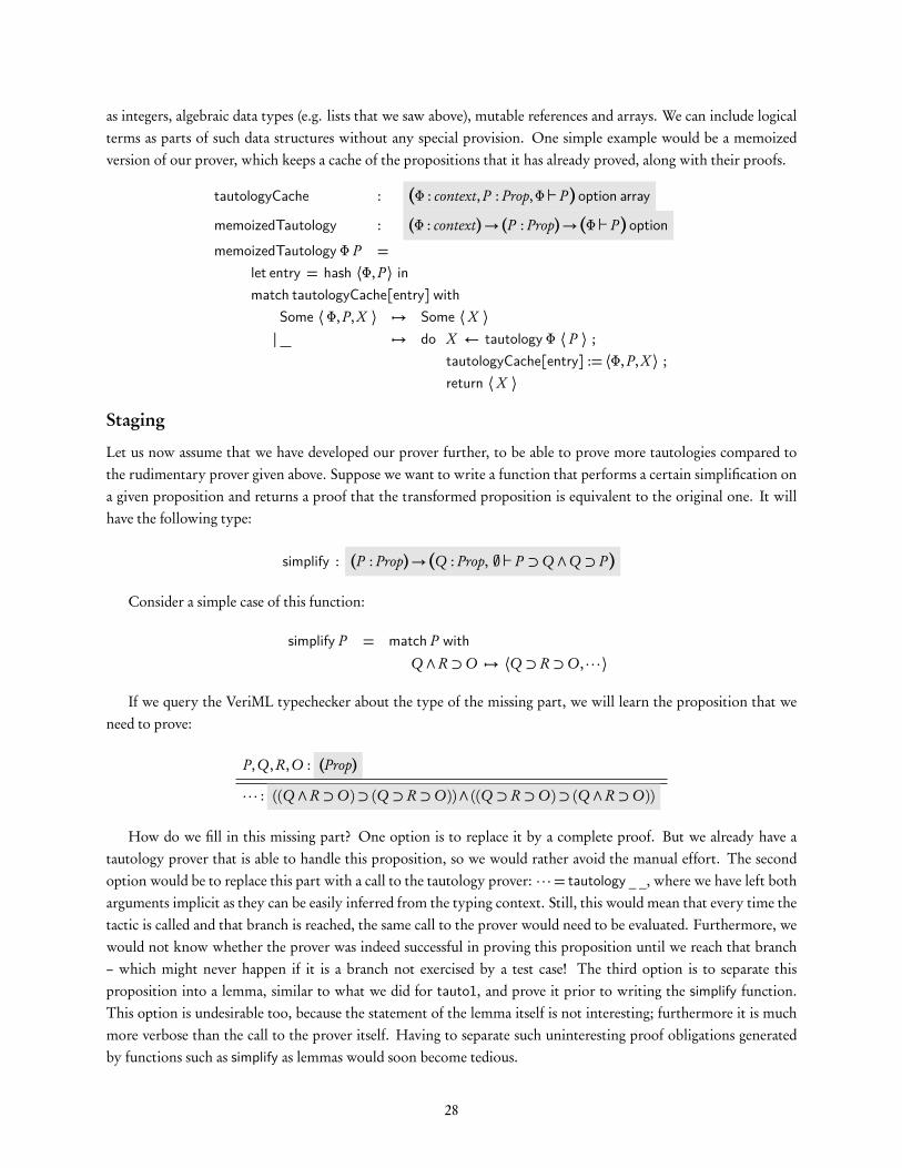
as integers, algebraic data types (e.g. lists that we saw above), mutable references and arrays. We can include logicalterms as parts of such data structures without any special provision. One simple example would be a memoizedversion of our prover, which keeps a cache of the propositions that it has already proved, along with their proofs.

tautologyCache : (Φ : context, P : Prop,Φ ` P) option array

memoizedTautology : (Φ : context)→ (P : Prop)→ (Φ ` P) optionmemoizedTautology Φ P =

let entry = hash ⟨Φ, P ⟩ inmatch tautologyCache[entry]with

Some ⟨Φ, P,X ⟩ 7→ Some ⟨X ⟩| 7→ do X ← tautology Φ ⟨ P ⟩ ;

tautologyCache[entry] := ⟨Φ, P,X ⟩ ;return ⟨X ⟩

Staging

Let us now assume that we have developed our prover further, to be able to prove more tautologies compared tothe rudimentary prover given above. Suppose we want to write a function that performs a certain simplification ona given proposition and returns a proof that the transformed proposition is equivalent to the original one. It willhave the following type:

simplify : (P : Prop)→ (Q : Prop, ; ` P ⊃Q ∧Q ⊃ P)

Consider a simple case of this function:

simplify P = match P withQ ∧R⊃O 7→ ⟨Q ⊃ R⊃O, · · · ⟩

If we query the VeriML typechecker about the type of the missing part, we will learn the proposition that weneed to prove:

P,Q, R,O : (Prop)

· · · : ((Q ∧R⊃O)⊃ (Q ⊃ R⊃O))∧ ((Q ⊃ R⊃O)⊃ (Q ∧R⊃O))

How do we fill in this missing part? One option is to replace it by a complete proof. But we already have atautology prover that is able to handle this proposition, so we would rather avoid the manual effort. The secondoption would be to replace this part with a call to the tautology prover: · · ·= tautology _ _, where we have left botharguments implicit as they can be easily inferred from the typing context. Still, this would mean that every time thetactic is called and that branch is reached, the same call to the prover would need to be evaluated. Furthermore, wewould not know whether the prover was indeed successful in proving this proposition until we reach that branch– which might never happen if it is a branch not exercised by a test case! The third option is to separate thisproposition into a lemma, similar to what we did for tauto1, and prove it prior to writing the simplify function.This option is undesirable too, because the statement of the lemma itself is not interesting; furthermore it is muchmore verbose than the call to the prover itself. Having to separate such uninteresting proof obligations generatedby functions such as simplify as lemmas would soon become tedious.

28

In VeriML we can solve this issue through the use of staging. We can annotate expressions so that they are staged– they are evaluated during a phase of evaluation that happens after typing but before runtime. These expressionscan be inside functions as well, yet they are still evaluated at the time that these functions are defined. Through thisapproach, we get the benefits of the separation into lemmas approach but with the conciseness of the direct call tothe prover. The example code would look as follows. We use brackets as the staging annotation for expressions.

simplify P = match P withQ ∧R⊃O 7→ ⟨Q ⊃ R⊃O,{tautology _ _}⟩

After type checking, this expression is made equivalent to the following, where the missing arguments are filledin based on the typing information.

simplify P = match P withQ ∧R⊃O 7→ ⟨Q ⊃ R⊃O,{tautology ; S}⟩

where S = ((Q ∧R⊃O)⊃ (Q ⊃ R⊃O))∧ ((Q ⊃ R⊃O)⊃ (Q ∧R⊃O))

After the static evaluation phase, the staged expression gets replaced by the proof that is returned by the tautol-ogy prover.

simplify P = match P withQ ∧R⊃O 7→ ⟨Q ⊃ R⊃O,X ⟩

where X =...; ` S

where S = ((Q ∧R⊃O)⊃ (Q ⊃ R⊃O))∧ ((Q ⊃ R⊃O)⊃ (Q ∧R⊃O))

Proof erasure

The last feature of VeriML that we will consider is proof erasure. Based on the type safety of the language, we knowthat expressions of a certain type will indeed evaluate to values of the same type, if successful. For example, consideran expression that uses functions such as tautology in order to prove a proposition P : if the expression does evaluateto a result (instead of diverging or throwing an exception), that result will be a valid proof of P .

We have said that we are able to pattern match on logical terms such as propositions and proofs. If we relax thisso that we cannot pattern match on proof terms, type safety can give us the further property of proof-erasure: if wedelete all proofs from our VeriML expressions and proceed to evaluate these expressions normally, their runtimebehavior is exactly the same as before the deletion – other than the space savings of not having to realize the proofsas data in the computer memory. Therefore, even if we do not generate these proofs, valid proof objects are stillguaranteed to exist. Relaxing the pattern matching construct as such is not a serious limitation, as we are notinterested in the particular structure of a proof but only on its existence.

For purposes of our discussion, we will show what the proof-erased version of the prover we have written abovewould look like.

29

tautology : (Φ : context)→ (P : Prop)→ unit optiontautology Φ P = match P with

Q ∧R 7→ do tautology ΦQ ;tautology Φ R ;return ()

|Q ∨R 7→ (do tautology ΦQ ;return ()) ||

(do tautology Φ R ;return ())

|Q ⊃ R 7→ do tautology (Φ, Q) R ;return ()

This code looks very similar to what we would write in a normal ML function that did not need to produceproofs. This equivalence is especially evident if we keep in mind that unit option is essentially the boolean type,monadic composition corresponds to boolean AND, monadic return to boolean true and the || operation to booleanOR.

The space savings associated with proof erasure are considerable, especially in the case of functions that are usedubiquitously in order to produce proofs, such as the small-scale automation mechanisms that we mentioned earlier inthis chapter. Still, full proof erasure means that we have to completely trust the VeriML implementation. Instead wewill use proof erasure selectively, e.g. in order to evaluate the functions comprising the conversion rule, enlargingthe trusted base only by the proof-erased versions of those functions. Yet a receiver of a VeriML proof can chooseto re-evaluate these functions without proof erasure and get complete proofs without missing parts. Therefore thetrusted base of our system is not decided at the design time of the logic we are going to use, but at the sites of thereceivers of the proofs. This allows a wide range of possibilities in choosing between the level of rigor requiredand the cost associated with proof checking, and is a significant advancement from the traditional way of handlingproofs as certificates sent to a third party.

Last, we would like to briefly comment on the fact that the combination of proof erasure with the stagingannotation is very powerful, as it allows us to extend the notion of what constitutes a valid proof. Take the followingsketch of a proof as an example:

*

...(x + y)2 > 0 {arith _ _} : (x + y)2 = x2+ 2xy + y2

x2+ 2xy + y2 > 0

+

In this proof, we use the automated arithmetic prover arith to validate a simple algebraic identity. By using prooferasure for this call, no proof object for this identity is ever generated – yet we are still guaranteed that a proof thatuses only the initial logical rules (plus axioms of arithmetic) exists. Furthermore, this identity is validated statically:if we use the above proof inside a function such as tautology to fill in the proof obligations (as we did for · · ·1 earlier),we will still know that the whole proof is valid at the time that the function is defined. This is due to staging thecall to the arith function. This process roughly corresponds to extending the available logical rules with calls toproof-producing functions; yet we maintain the property that we can statically validate these “extended” proofs.The fact that no evidence needs to be produced, means that we can effectively hide these trivial details – both interms of user effort required, and of the cost of validating them.

Yet the automation functions handling these trivial details are developed in VeriML, which means that we can

30

develop better versions of them in the same language to handle further details or further domains. Thus our ap-proach to small-scale automation departs from the traditional approach of hardcoding fixed small-scale automationmechanisms in the core implementation of the proof assistant; it enables instead layered development of increas-ingly more sophisticated small-scale automation, in a manner resembling the informal practice of acquiring furtherintuition.

31

Chapter 3

The logic λHOL: Basic framework

In this chapter we will present the details of the λHOL logic that VeriML uses.

3.1 The base λHOL logic

The logic that we will use is a simple type-theoretic higher-order logic with explicit proof objects. This logic wasfirst introduced in Barendregt and Geuvers [1999] and can be seen as a shared logical core between CIC [Coquandand Huet, 1988, Bertot et al., 2004] and the HOL family of logics as used in proof assistants such as HOL4 [Slindand Norrish, 2008], HOL-Light [Harrison, 1996] and Isabelle/HOL [Nipkow et al., 2002]. It is a constructivelogic yet admits classical axioms.

The logic is composed of the following classes:

– The objects of the domain of discourse, denoted d : these are the objects that the logic reasons about, suchas natural numbers, lists and functions between such objects.

– The propositions, denoted as P : these are the statements of the logic. As this is a higher-order logic, proposi-tions themselves are objects of the domain of discourse d , having a special Prop type. We use P instead of dwhen it is clear from the context that a domain object is a proposition.

– The kinds, denoted K: these are the types that classify the objects of the domain of discourse, including theProp type for propositions.

– The sorts, denoted s , which are the classifiers of kinds.

– The proof objects, denoted π, which correspond to a linear representation of valid derivations of proposi-tions.

– The variables context, denoted Φ, which is a list of variables along with their type.

– The signature, denoted Σ, which is a list of axioms, each one corresponding to a constant and its type.

The syntax of these classes is given in Figure 3.1, while the typing judgements of the logic are given in Figures3.2 and 3.3. We will now comment on the term formers and their associated typing rules.

The proposition P1 → P2 denotes logical implication whereas the kind former K1 → K2 is inhabited by totalfunctions between domain objects. Both use the standard forms of lambda abstraction and function application as

32

(sorts) s ::= Type | Type′

(kinds) K ::= Prop | cK | K1→K2(dom.obj. and prop.) d , P ::= P1→ P2 | ∀x : K.P | λx : K.d | d1 d2 | x | cd

(proof objects) π ::= λx : P.π | π π′ | λx : K.π | π d | x | cπ(variable contexts) Φ ::= • | Φ, x : Type | Φ, x : K | Φ, x : P

(constant signature) Σ ::= • | Σ, cK : Type | Σ, cd : K | Σ, cπ : P

Figure 3.1: The base syntax of the logic λHOL

`Σwf well-formedness of signatures`Σ Φwf well-formedness of contextsΦ `Σ K : Type well-formedness for kindsΦ `Σ d : K kinding of domain objectsΦ `Σ π : P valid logical derivations of proof objects proving a proposition

`Σwf

` •wf`Σwf cK : Type 6∈Σ`Σ, cK : Type wf

`Σwf • `Σ K : Type cd : _ 6∈Σ`Σ, cd : K wf

`Σwf • `Σ P : Prop cπ : _ 6∈Σ`Σ, cπ : P wf

`Σ Φwf

` •wf

` Φwf

` Φ, x : Type wf

` Φwf Φ `K : Type

` Φ, x : K wf

` Φwf Φ ` P : Prop

` Φ, x : P wf

Φ `Σ K : Type

Φ ` Prop : Type

cK : Type ∈ΣΦ `Σ cK : Type

Φ `K1 : Type Φ `K2 : Type

Φ `K1→K2 : Type

Φ `Σ d : K

Φ ` P1 : Prop Φ ` P2 : Prop

Φ ` P1→ P2 : Prop

Φ `K : Type Φ, x : K ` P : Prop

Φ ` ∀x : K.P : Prop

Φ `K : Type Φ, x : K ` d : K′

Φ ` λx : K.d : K→K′

Φ ` d1 : K′→K Φ ` d2 : K′

Φ ` d1 d2 : K

x : K ∈ΦΦ ` x : K

cd : K ∈ΣΦ `Σ cd : K

Figure 3.2: The typing rules of the logic λHOL

33

Φ `Σ π : P

Φ ` P : Prop Φ, x : P `π : P ′

Φ ` λx : P.π : P → P ′→INTRO

Φ `π1 : P ′→ P Φ `π2 : P ′

Φ `π1 π2 : P→ELIM

Φ `K : Type Φ, x : K `π : P

Φ ` λx : K.π : ∀x : K.P∀INTRO

Φ `π : ∀x : K.P Φ ` d : KΦ `π d : P[d/x]

∀ELIMx : P ∈ΦΦ ` x : P

VAR

cπ : P ∈ΣΦ `Σ cπ : P

CONSTANT

Figure 3.3: The typing rules of the logic λHOL (continued)

fv(d )

fv(P1→ P2) = fv(P1)∪ fv(P2)fv(∀x : K.P ) = fv(P ) \ {x}fv(λx : K.d ) = fv(d ) \ {x}fv(d1 d2) = fv(d1)∪ fv(d2)fv(x) = {x}fv(cd ) = ;

d[d ′/x]

(P1→ P2)[d/x] = P1[d/x]→ P2[d/x](∀y : K.P )[d/x] = ∀y : K.P[d/x] when fv(P )∩ fv(d ) = ; and x 6= y(λy : K.d ′)[d/x] = λy : K.d ′[d/x] when fv(d ′)∩ fv(d ) = ; and x 6= y(d1 d2)[d/x] = d1[d/x] d2[d/x](x)[d/x] = d(y)[d/x] = y(cd )[d/x] = cd

Figure 3.4: Capture avoiding substitution

34

their introduction and elimination rules. In the case of the proposition P1 → P2, the typing rules for the proofobjects λx : P1.π and π1 π2 correspond exactly to the introduction and elimination rules for logical implicationas we gave them in Section 2.3; the proof objects are simply a way to record the derivation as a term instead of atree. The proposition ∀x : K.P denotes universal quantification. As K includes a domain former for propositionsand functions yielding propositions, we can quantify over propositions and predicates. This is why λHOL is ahigher-order logic – for example, it is capable of representing natural number induction as the proposition:

∀P : Nat→ Prop.P 0→ (∀n : Nat, P n→ P (succ n))→∀n : Nat, P n

When a quantified formula ∀x.P is instantiated with an object d using the rule ∀ELIM, we get a proof of P[d/x].The notation [d/x] represents standard capture-avoiding substitution, defined in Figure 3.4.

There are three different types of constants; their types are determined from the signature context. Constantsdenoted as cK correspond to the domains of discourse such as natural numbers (written as Nat), ordinals (written asOrd) and lists (written as List). Constant domain objects, denoted as cd are used for constructors of these domains(for example, zero : Nat and succ : Nat → Nat for natural numbers); for functions between objects (for example,plus : Nat→ Nat→ Nat for the addition function of natural numbers); for predicates (e.g. le : Nat→ Nat→ Propfor representing when one natural number is less-than-or-equal to another); and for logical connectives, which areunderstood as functions between propositions (e.g. logical conjunction, represented as and : Prop→ Prop→ Prop).Constant proof objects, denoted as cπ, correspond to axioms. The constants above get their expected meaningby adding their corresponding set of axioms to the signature – for example, logical conjunction has the followingaxioms:

andIntro : ∀P1, P2 : Prop.P1→ P2→ and P1 P2

andElim1 : ∀P1, P2 : Prop.and P1 P2→ P1

andElim2 : ∀P1, P2 : Prop.and P1 P2→ P2

Our logic supports inductive definitions of domains and predicates, in a style similar to CIC. We do not representthem explicitly in the logic, opting instead for viewing such definitions as generators of a number of ‘safe to add’constants. The logic we have presented – along with the additions made below – is a subset of CIC. It has been shownin Werner [1994] that CIC is a consistent logic; thus it is understood that the logic we present is also consistent,when the signature Σ is generated only through such inductive definitions. We will present more details aboutinductive definitions after we make some extensions to the core of the logic that we have presented so far.A simple example of a proof object for commutativity of conjunction follows.

λP : Prop.λQ : Prop.λH : ∧ P Q.andIntro Q P (andElim2 P Q H ) (andElim1 P Q H )

Based on the typing rules, it is simple to show that it proves the proposition:

∀P : Prop.∀Q : Prop.and P Q→ and Q P

3.2 Adding equality

The logic we have presented so far is rather weak when it comes to reasoning about the total functions inhabitingK1→K2. For example, we cannot prove that the standard β-reduction rule:

(λx : K.d ) d ′ = d[d ′/x]

35

Moreover, consider the case where we have a proof of a proposition such as P (1+1). We need to be able to constructa proof of P (2) out of this, yet the logic we have presented so far does not give us this ability.

There are multiple approaches for adding rules to logics such as λHOL in order to make equality behave inthe expected way. In order to understand the differences between these approaches, it is important to distinguishtwo separate notions of equality in a logic: definitional equality and propositional equality. Definitional equalityrelates terms that are indistinguishable from each other in the logic. Proving that two definitionally equal termsare equal is trivial through reflexivity, since they are viewed as exactly the same terms. We will use d1 ≡ d2 torepresent definitional logic. Propositional equality is an actual predicate of the logic. Terms are proved to bepropositionally equal using the standard axioms and rules of the logic. In λHOL we would represent propositionalequality through propositions of the form d1 = d2. With this distinction in place, we will give a brief summary ofthe different approaches below.

Explicit equality. In the HOL family of logics, as used in systems like HOL4 [Slind and Norrish, 2008] and Is-abelle/HOL [Nipkow et al., 2002], definitional equality is just syntactic equality. Any equality further thanthat is propositional equality and needs to be proved using the logic. The logic includes a rule where proposi-tions that can be proved equal can replace each other as the type of proof objects. Any such rewriting needsto be witnessed in the resulting proof objects. A sketch of the typing rule for this axiom is the following:

Φ `π : P Φ `π′ : P = P ′

Φ ` convπ π′ : P ′

The advantage of this approach is that a type checker for it only has to check proofs that contain all therequired details about why terms are equal. It is therefore extremely simple, keeping the trusted base of ourlogic as simple as possible. Still, it has a big disadvantage: the proof objects are very large, as even trivialequalities need to be painstakingly proved. It is possible that this is one of the reasons why systems based onthis logic do not generate proof objects by default, even though they all support them.

Intensional type theories. Systems based on Martin-Löf intensional type theory, such as Coq [Barras et al., 2012]and Agda [Norell, 2007], have an extended notion of definitional equality. In these systems, definitionalequality includes terms that are identical up to evaluation of the total functions used inside the logical terms.In order to make sure that the soundness of the logic is not compromised, this notion of evaluation needs tobe decidable. As we have said, terms that are definitionally equal are indistinguishable, so their equality doesnot need to be witnessed inside proof objects, resulting in a big reduction in their size.

The way that this is supported in such type theories is to define an equality relation R based on some fixed,confluent rewriting system. In Coq and Agda this includesβ-conversion and ι-conversion (evaluation of totalrecursive functions), pattern matching and unfolding of definitions. This equality relation is then understoodas the definitional equality, by adding the following conversion rule to the logic:

Φ `π : P1 P1 ≡R P2

Φ `π : P2

The benefit of this approach is that trivial arguments based on computation, which would normally not be“proved” in standard mathematical discourse, actually do not need to be proved and witnessed in the proofobjects. Therefore the logic follows what is called the Poincaré principle (e.g. in Barendregt and Geuvers

36

[1999]). One disadvantage of this approach is that our trusted base needs to be bigger, since a type-checkerfor such a logic needs to include a decision procedure for the relation R.

Extensional type theories. In extensional type theories like NuPRL [Constable et al., 1986], the notion of defini-tional equality and propositional equality are identified. That means that anything that can be proved equalin the logic is seen implicitly as equal. A typing rule that sketches this idea would be the following:

Φ `π : P1 Φ `π′ : P1 = P2

Φ `π : P2

The advantage of this approach is that the size of proof objects is further reduced, bringing them even closerto normal mathematical practice. Still, theories with this approach have a big disadvantage: type-checkingproof objects becomes undecidable. It is easy to see why this is so from the above typing rule, as the π′ proofobject needs to be reconstructed from scratch during type checking time – that is, type checking depends onbeing able to decide whether two arbitrary terms are provably equal or not, an undecidable problem in anymeaningful logic. Implementations of such theories deal with this by only implementing a set of decisionprocedures that can decide on such equalities, but all of these procedures become part of the trusted base ofthe system.

We should note here that type theories such as CIC and NuPRL support a much richer notion of domain objectsand kinds, as well as a countable hierarchy of universes above the Type sort that we support. For example, kindsthemselves can be computed through total functions. In these cases, the chosen approach with respect to equalityalso affects which terms are typable. Our logic is much simpler and thus we will only examine equality at the levelof domain objects. Still, we believe that the techniques we develop are applicable to these richer logics and to caseswhere equality at higher universes such as the level of kinds K is also available.

We want λHOL to have the simplest possible type checker, so we choose the explicit equality version. We willsee how to recover and extend the benefits of the conversion rule through VeriML in Section 7.1. We thereforeextend our logic with a built-in propositional equality predicate, as well as a set of equality axioms. The extensionsrequired to the logic presented so far are given in Figure 3.5. We sometimes refer to λHOL together with theseextensions as λHOLE in order to differentiate with a version that we will present later which includes the conversionrule; that version is called λHOLC .

Most of the typing rules of the new axioms are standard. We have an explicit axiom forβ-reduction through theproof object constructor beta. α-equivalence is handled informally at this level by implicitly identifying terms thatare equal up to renaming of bound variables; this will be changed in the next section. Note that some rules seemto omit certain premises, such as the fact that P2 is a proposition in the case of congForall. The reason is that thesepremises are always true based on the existing ones; in the example at hand, the fact that P1 = P2 implies that theirtype is identical, thus P2 is a proposition just like P1 is.

The given set of axioms is enough to prove other expected properties of equality, such as symmetricity:

symmK : ∀a : K.∀b : K.a = b → b = asymmK = λa : K.λb : K.λH : a = b . conv(refl a) (subst (x : K.x = a)H )

3.3 λHOL as a Pure Type System

Our presentation of λHOL above separates the various different types of logical terms into distinct classes. Thisseparation results in duplicating various typing rules – for example, quantification, logical implication and function

37

Syntax extensions

(dom.obj. and prop.) d , P ::= · · · | d1 = d2(proof objects) π ::= refl d | convπ π′ | subst (x : K.P )π | congLam (x : K.π)

| congForall (x : K.π) | beta (x : K.d ) d ′

Φ `Σ d : K

Φ ` d1 : K Φ ` d2 : KΦ ` d1 = d2 : Prop

Φ `Σ π : P

Φ ` d : KΦ ` refl d : d = d

Φ `π : P Φ ` P : Prop Φ `π′ : P = P ′

Φ ` convπ π′ : P ′

Φ, x : K ` P : Prop Φ `π : d1 = d2 Φ ` d1 : KΦ ` subst (x : K.P )π : P[d1/x] = P[d2/x]

Φ, x : K `π : d1 = d2

Φ ` congLam (x : K.π) : (λx : K.d1) = (λx : K.d2)

Φ, x : K `π : P1 = P2 Φ, x : K ` P1 : Prop

Φ ` congForall (x : K.π) : (∀x : K.P1) = (∀x : K.P2)

Φ ` (λx : K.d ) : K→K′ Φ ` d ′ : KΦ ` beta (x : K.d ) d ′ : ((λx : K.d ) d ′) = (d[d ′/x])

Figure 3.5: The logic λHOLE : syntax and typing extensions for equality

(sorts) s ::= Prop | Type | Type′

(logical terms) t ::= s | x | c | ∀x : t1.t2 | λx : t1.t2 | t1 t2 | t1 = t2 | refl t| conv t1 t2 | subst (x : tk .tP ) t | congLam (x : tk .t )| congForall (x : tk .t ) | beta (x : tk .t1) t2

(variable contexts) Φ ::= • | Φ, x : t(constant signature) Σ ::= • | Σ, c : t

Figure 3.6: The syntax of the logic λHOL given as a PTS

38

`Σwf well-formedness of signatures`Σ Φwf well-formedness of contextsΦ `Σ t : t ′ typing of logical terms

`Σwf

` •wf`Σwf • `Σ t : s

`Σ, x : t wf

`Σ Φwf

` •wf` Φwf Φ ` t : s

` Φ, x : t wf

Φ `Σ t : t ′

(s , s ′) ∈AΦ ` s : s ′

Φ ` t1 : s Φ, x : t1 ` t2 : s ′ (s , s ′, s ′′) ∈RΦ ` ∀x : t1.t2 : s ′′

Φ ` t1 : ∀x : t .t ′ Φ ` t2 : t

Φ ` t1 t2 : t ′[t2/x]

Φ, x : t1 ` t2 : t ′ Φ ` ∀x : t1.t ′ : s

Φ ` λx : t1.t2 : ∀x : t1.t ′x : t ∈ΦΦ ` x : t

c : t ∈ΣΦ `Σ c : t

Φ ` t1 : t Φ ` t2 : t Φ ` t : Type

Φ ` t1 = t2 : Prop

Φ ` t : t ′ Φ ` t ′ : Type

Φ ` refl t : t = t

Φ ` t1 : t Φ ` t : Prop Φ ` t2 : t = t ′

Φ ` conv t1 t2 : t ′

Φ ` tk : Type Φ, x : tk ` tP : Prop Φ ` t : ta = tb Φ ` ta : tk

Φ ` subst (x : tk .tP ) t : tP [ta/x] = tP [tb/x]

Φ ` tk : Type Φ, x : tk ` t : t1 = t2

Φ ` congLam (x : tk .t ) : (λx : tk .t1) = (λx : tk .t2)

Φ ` tk : Type Φ, x : tk ` t : t1 = t2 Φ, x : tk ` t1 : Prop

Φ ` congForall (x : tk .t ) : (∀x : tk .t1) = (∀x : tk .t2)

Φ ` (λx : ta .t1) : ta→ tb Φ ` ta→ tb : Type Φ ` t2 : ta

Φ ` beta (x : ta .t1) t2 : ((λx : ta .t1) t2) = (t1[t2/x])

Figure 3.7: The typing rules of the logic λHOL in PTS style

39

kinds share essentially the same type and term formers. This needlessly complicates the rest of our development.We will now present λHOL as a Pure Type System [Barendregt, 1992] which is the standard way to describe typedlambda calculi. Essentially the syntactic classes of all logical terms given above are merged into one single class,denoted as t . We give the new syntax in Figure 3.6 and the new typing rules in Figure 3.7. Note that we use t1→ t2

as syntactic sugar for ∀x : t1.t2 when x does not appear free in t2.A PTS is characterized by three parameters: the set of sorts, the set of axioms and the set of rules. These parame-

ters are instantiated as follows for λHOL:

S = {Prop, Type, Type′}A = {(Prop,Type), (Type,Type′)}R = {(Prop,Prop,Prop), (Type,Type,Type), (Type,Prop,Prop)}

Terms sorted1 under Prop represent proofs, under Type represent objects (including propositions) and under Type′

represent the domains of discourse (e.g. natural numbers). The axiom (Prop,Type) corresponds to the fact thatpropositions are objects of the domain of discourse, while the axiom (Type,Type′) is essentially what allows us tointroduce constants and variables for domains. The rules are understood as logical implication, function formationbetween objects and logical quantification, respectively. Based on these parameters, it is evident that λHOL issimilar to System Fω, which is usually formulated as S = {?,�}, A = {(?,�)}, R = {(?,?,?), (�,�,�), (�,?,?)}.λHOL is a straightforward extension with an extra sort above � – that is, Type′ above Type – allowing us to havedomains other than the universe of propositions. Furthermore, λHOL extends the basic PTS system with thebuilt-in explicit equality as presented above, as well as with the signature of constants Σ.

The substitution lemma

The computational language of VeriML assumes a simple set of properties that need to hold for the type systemof the logic language. The most important of these is the substitution lemma, stating that substituting terms forvariables of the same type yields well-typed terms. We will prove a number of such substitution lemmas for differentnotions of ‘term’ and ‘variable’. As an example, let us state the substitution lemma for logical terms of λHOL inthe PTS version of the logic.

Lemma 3.3.1 (Substitution) If Φ, x : t ′T , Φ′ ` t : tT and Φ ` t ′ : t ′T then Φ, Φ′[t ′/x] ` t[t ′/x] : tT [t′/x].

The proof of the lemma is a straightforward induction on the typing derivation of the term t . The most importantauxiliary lemma it depends on is that typing obeys the weakening structural rule, that is:

Lemma 3.3.2 (Weakening) If Φ ` t : tT then Φ, x : t ′T ` t : tT .

The substitution lemma can alternatively be stated for a list of substitutions of variables to terms, covering thewhole context. This alternative statement is technically advantageous in terms of how the proof is carried throughand also how the lemma can be used. The lemma is stated as follows:

Lemma 3.3.3 (Simultaneous substitution) If x1 : t1, x2, t2, · · · , xn : tn ` t : tT and for all i with 1 ≤ i ≤ n,Φ′ ` xi : ti , then Φ′ ` t[t1, t2, · · · , tn/x1, x2, · · · , xn].

We can view the list of (xi , ti ) variable-term pairs as a well-typed substitution covering the context Φ. We will givea more precise definition of this notion in the following section.

1. That is, terms typed under a term whose sort is the one we specify.

40

For the rest of our development, we will switch to a different variable representation, which will allow us tostate these lemmas more precisely, by removing the dependence on variable names and the requirement for implicitα-renaming in the definition of substitution. Thus we will not go into more details of these proofs as stated here.

3.4 λHOL using hybrid deBruijn variables

So far, we have used names to represent variables in λHOL. Terms that are equivalent up to α-renaming are deemedto be exactly the same and are used interchangeably. An example of this shows up in the definition of capture-avoiding substitution in Figure 3.4: constructs that include binders, such as λy : K.d , are implicitly α-renamed sothat no clashes with the variables of the subsitutend are introduced. We are essentially relying on viewing termsas representatives of their α-equivalence classes; our theorems would also reason up to this equivalence. It is awell-known fact [Aydemir et al., 2008] that when formally proving such theorems about languages with binding inproof assistants, identifying terms up to α-equivalence poses a large number of challenges. This is usually addressedby choosing a concrete variable representation technique where the non-determinism of choosing variable names isremoved and thus all α-equivalent terms are represented in the same way.

We have found that using a similar concrete variable representation technique is advantageous for our devel-opment, even though our proofs are done on paper. The main reason is that the addition of contextual terms,contextual variables and polymorphic contexts introduces a number of operations which are hard to define in thepresence of named variables, as they trigger complex sets of α-renamings. Using a concrete representation, theseoperations and the renamings that are happening are made explicit. Furthermore, we use the same concrete rep-resentation in our implementation of VeriML itself, so the gap between the formal development and the actuallyimplemented code is smaller, increasing our confidence in the overall soundness of the system.

The concrete representation technique that we use is a novel, to the best of our knowledge, combination of thetechniques of de Bruijn indices, de Bruijn levels [De Bruijn, 1972] and the locally nameless approach [McKinna andPollack, 1993]. The former two techniques replace all variables by numbers, whereas the locally nameless approachintroduces a distinction between bound and free variables and handles them differently. Let us briefly summarizethese approaches before presenting our hybrid representation. A table comparison is given in Table 3.1. DeBruijnindices correspond to the number of binders above the current variable reference where the variable was bound.DeBruijn levels are the “inverse” number, corresponding to how many binders we have to cross until we reach theone binding the variable we are referring to, if we start at the top of the term. Both treat free variables by consideringthe context as a list of variable binders. In both cases, when performing the substitution (λy.t )[t ′/x], we need toshift the variable numbers in t ′ in order for the resulting term to be well-formed – the free variables in the indicescase or the bound variables in the levels case. In the indices case, the introduction of the new binder alters the wayto refer to the free variables (the free variable represented by index n in t ′ will be represented by n + 1 under theλ-abstraction), as the identities of free variables directly depend on the number of bound variables at a point. Inthe levels case, what is altered is the way we refer to bound variables within t ′ – the ‘allocation policy’ for boundvariables in a way. For example the lambda term t ′ = λx.x that was represented as λ.n outside the new binder isnow represented as λ.n+ 1. This is problematic: substitution is not structurally recursive and needs to be reasonedabout together with shifting. This complicates both the statements and proofs of related lemmas.

The locally nameless approach addresses this problem by explicitly separating free from bound variables. Freevariables are represented normally using names whereas deBruijn indices are reserved for representing bound vari-ables. In this way the identities of free variables are preserved when a new binder is introduced and no shifting needsto happen. We still need two auxiliary operations: freshening, in order to open up a term under a binder into a term

41

Example of performing the substitution:(λy : x. f y a)[(λz : x.z) y/a]

Free variables context:x : Type, g : x→ x→ x, y : x, a : x

Named representation (λy : x.g y a)[(λz : x.z) y/a](λw : x.g w a)[(λz : x.z) y/a] =αλw : x.g w ((λz : x.z) y) ⇒

deBruijn indices (λ(3).3 0 1)[(λ(3).0) 1/0]λ(3).3 0 (shiftFree ((λ(3).0) 1)) ⇒λ(3).3 0 ((λ(4).0) 2) ⇒

deBruijn levels (λ(0).1 4 3)[(λ(0).4) 2/3]λ(0).1 4 (shiftBound ((λ(0).4) 2)) ⇒λ(0).1 4 ((λ(0).5) 2) ⇒

Locally nameless (λ(x).g 0 a)[(λ(x).0) y/a]λ(x).g 0 ((λ(x).0) y) ⇒

Hybrid deBruijn (λ(v0).v1 b0 v3)[(λ(v0).b0) v2/v3]λ(v0).v1 b0 ((λ(v0).b0) v2) ⇒

Table 3.1: Comparison of variable representation techniques

s ::= Prop | Type | Type′

t ::= s | c | vi | bi | λ(t1).t2 | t1 t2 | Π(t1).t2 | t1 = t2 | conv t1 t2| subst ((tk ).tP ) t | refl t | congLam ((tk ).t )| congForall ((tk ).t ) | beta ((tk ).t1) t2

Σ ::= • | Σ, c : tΦ ::= • | Φ, tσ ::= • | σ , t

Figure 3.8: The logic λHOL with hybrid deBruijn variable representation: Syntax

that has an extra free variable by replacing the dangling bound variable, and binding, which is the inverse operation,turning the last-introduced free variable into a bound variable, so as to close a term under a binder. Under thisapproach, not all α-equivalent terms are identified, as using different names for free variables in the context stillyields different terms.

We merge these approaches in a new technique that we call hybrid deBruijn variables: following the locallynameless approach, we separate free variables from bound variables and use deBruijn indices for bound variables(denoted as bi in Table 3.1); but also, we use deBruijn levels for free variables instead of names (denoted as vi ).In this way, all α-equivalent terms are identified. Furthermore, terms preserve their identity under additions tothe end of the free variables context. Such additions are a frequent operation in VeriML, so this representation isadvantageous from an implementation point of view. A similar representation technique where terms up to anyweakening of the context are identified (not just additions to the end of the context) by introducing a distinctionbetween used and unused variable names has been discovered independently by Pollack et al. [2011] and Pouillard[2011].

Let us now proceed to the presentation of λHOL using our hybrid representation technique. We give the newsyntax of the language in Figure 3.8, the new typing rules in Figures 3.9 and 3.10 and the definition of syntacticoperations in Figures 3.11, 3.12 and 3.13.

42

`Σwf

` •wfSIGEMPTY

`Σwf • `Σ t : s (c : _) 6∈Σ`Σ, c : t wf

SIGCONST

`Σ Φwf

` •wfCTXEMPTY

` Φwf Φ ` t : s

` Φ, t wfCTXVAR

Φ ` σ : Φ′

` Φwf

Φ ` • : •SUBSTEMPTY

Φ ` σ : Φ′ Φ ` t : t ′ ·σΦ ` σ , t : (Φ′, t ′)

SUBSTVAR

Φ `Σ t : t ′

c : t ∈ΣΦ `Σ c : t

CONSTANTΦ.i = t

Φ ` vi : tVAR

(s , s ′) ∈AΦ ` s : s ′

SORT

Φ ` t1 : s Φ, t1 ` dt2e|Φ| : s ′ (s , s ′, s ′′) ∈R

Φ `Π(t1).t2 : s ′′ΠTYPE

Φ ` t1 : s Φ, t1 ` dt2e|Φ| : t ′ Φ `Π(t1).�

t ′�

|Φ|+1 : s ′

Φ ` λ(t1).t2 :Π(t1).�

t ′�

|Φ|+1

ΠINTROΦ ` t1 :Π(t ).t ′ Φ ` t2 : t

Φ ` t1 t2 :�

t ′�

|Φ| · (idΦ, t2)ΠELIM

Φ ` t1 : t Φ ` t2 : t Φ ` t : Type

Φ ` t1 = t2 : PropEQTYPE

Figure 3.9: The logic λHOL with hybrid deBruijn variable representation: Typing Judgements

43

Φ ` t1 : t Φ ` t1 = t1 : Prop

Φ ` refl t1 : t1 = t1

EQREFLΦ ` t : t1 Φ ` t1 : Prop Φ ` t ′ : t1 = t2

Φ ` conv t t ′ : t2

EQELIM

Φ ` tk : Type Φ, tk ` dtP e|Φ| : Prop Φ ` t : ta = tb Φ ` ta : tk

Φ ` subst ((tk ).tP ) t : tP · (idΦ, ta) = tP · (idΦ, tb )EQSUBST

Φ ` tk : Type Φ, tk ` dte|Φ| : t1 = t2

Φ ` congLam ((tk ).t ) : (λ(tk ).bt1c|Φ|+1) = (λ(tk ).bt2c|Φ|+1)EQLAM

Φ ` tk : Type Φ, tk ` dte|Φ| : t1 = t2 Φ, tk ` t1 : Prop

Φ ` congForall ((tk ).t ) : (∀(tk ).bt1c|Φ|+1) = (∀(tk ).bt2c|Φ|+1)EQFORALL

Φ ` (λ(ta).t1) : ta→ tb Φ ` ta→ tb : Type Φ ` t2 : ta

Φ ` beta ((ta).t1) t2 : ((λ(ta).t1) t2) = dt1e|Φ| · (idΦ, t2)EQBETA

Figure 3.10: The logic λHOL with hybrid deBruijn variable representation: Typing Judgements (continued)

As expected, the main change to the syntax of terms and of the context Φ is that binding structures do not carryvariable names any longer. For example, instead of writing λx : t1.t2 we now write λ(t1).t2. In the typing rules, themain change is that extra care needs to be taken when going into a binder or when enclosing a term with a binder.This is evident for example in the rules ΠTYPE and ΠINTRO. When we cross a binder, the just-bound variable b0

needs to be converted into a fresh free variable. This is what the freshening operation dtenm does, defined in Figure3.11. The two arguments are as follows: n represents which bound variable to replace and is initially 0 when weleave it unspecified; m is the current number of free variables (the length of the current context), so that the nextfresh free variable vm is used as the replacement of the bound variable. Binding is the inverse operation and is usedwhen we are re-introducing a binder, capturing the last free variable and making it a bound variable. The argumentsare similar: n represents which bound variable to replace with and m represents the level of the last free variable.

As is evident in the above discussion, the operations of freshening and binding have particular assumptionsabout the terms they are applied to. For example, freshening needs to be applied to a term with one “dangling”bound variable, whereas binding needs to be applied to a closed term. In order to state such assumptions precisely,we define the notion of free and bound variable limits in Figure 3.12. We say that a term t obeys the limit of n freevariables, and write t < f n when t does not contain any free variable higher than vn−1. Bound variable limits aresimilar.

We have also changed the way we denote and perform substitutions. We have added simultaneous substitutionsas a new syntactic class. We denote them as σ and refer to them simply as substitutions from now on. Theyrepresent lists of terms to substitute for the variables in a Φ context. Notice that the lack of variable names requiresthat both Φ and σ are ordered lists rather than sets. The order of a substitution σ needs to match the order of thecontext that it corresponds to. This is made clear in the definition of the operation of applying a substitution to aterm, written as t ·σ and given in Figure 3.13. In essence, substitution application is a simple structural recursion,the only interesting case2 being the replacement of the i -th free variable with the i -th term of the substitution. It isevident that substitution cannot be applied to terms that use more free variables than there are in the substitution.

2. As a notational convenience, we mark such interesting cases with a star.

44

Freshening: dtenm

dsenm = sdcenm = c

∗ dvienm = vi

∗ dbnenm = vm

dbienm = bi

d(λ(t1).t2)enm = λ(dt1e

nm).dt2e

n+1m

dt1 t2enm = dt1e

nm dt2e

nm

dΠ(t1).t2)enm = Π(dt1e

nm).(dt2e

n+1m )

dt1 = t2enm = dt1e

nm = dt2e

nm

dconv t1 t2enm = conv dt1e

nm dt2e

nm

drefl tenm = refl dtedsubst (tk .tP ) tenm = subst (dtke

nm .dtP e

n+1m ) dtenm

dcongLam (tk .t )enm = congLam (dtkenm .dten+1

m )dcongForall (tk .t )enm = congForall (dtke

nm .dten+1

m )dbeta (tk .t1) t2e

nm = beta (dtke

nm .dt1e

n+1m ) dt2e

nm

Binding: btcnm

bscnm = sbccnm = c

∗�

vm−1�n

m = bn∗ bvic

nm = vi

bbicnm = bi

b(λ(t1).t2)cnm = λ(bt1c

nm).bt2c

n+1m

bt1 t2cnm = bt1c

nm bt2c

nm

bΠ(t1).t2)cnm = Π(bt1c

nm).bt2c

n+1m

bt1 = t2cnm = bt1c

nm = bt2c

nm

bconv t1 t2cnm = conv bt1c

nm bt2c

nm

brefl tcnm = refl btcnmbsubst (tk .tP ) tcnm = subst (btkc

nm .btP c

n+1m ) btcnm

bcongLam (tk .t )cnm = congLam (btkcnm .btcn+1

m )bcongForall (tk .t )cnm = congForall (btkc

nm .btcn+1

m )bbeta (tk .t1) t2c

nm = beta (btkc

nm .bt1c

n+1m ) bt2c

nm

Figure 3.11: The logic λHOL with hybrid deBruijn variable representation: Freshening and Binding

45

Free variable limits for terms:t < f n

s < f nc < f nvi <

f n ⇐ n > ibi <

f n(λ(t1).t2)<

f n ⇐ t1 <f n ∧ t2 <

f nt1 t2 <

f n ⇐ t1 <f n ∧ t2 <

f n· · ·

Free var. limits for substitutions:σ < f n

•< f n(σ , t )< f n ⇐ σ < f n ∧ t < f n

Bound var. limits for terms:t <b n

s <b nc <b nvi <

b nbi <

b n ⇐ n > i(λ(t1).t2)<

b n ⇐ t1 <b n ∧ t2 <

b n+ 1t1 t2 <

b n ⇐ t1 <b n ∧ t2 <

b n· · ·

Bound var. limits for substitutions:σ <b n

•<b n(σ , t )<b n ⇐ σ <b n ∧ t <b n

Figure 3.12: The logic λHOL with hybrid deBruijn variable representation: Variable limits

Substitution application: t ·σ

s ·σ = sc ·σ = c

∗ vi ·σ = σ .ibi ·σ = bi(λ(t1).t2) ·σ = λ(t1 ·σ).(t2 ·σ)(t1 t2) ·σ = (t1 ·σ) (t2 ·σ)(Π(t1).t2) ·σ = Π(t1 ·σ).(t2 ·σ)(t1 = t2) ·σ = (t1 ·σ) = (t2 ·σ)(conv t1 t2) ·σ = conv (t1 ·σ) (t2 ·σ)(refl t ) ·σ = refl (t ·σ)(subst (tk .tP ) t ) ·σ = subst (tk ·σ .tP ·σ) (t ·σ)(congLam (tk .t )) ·σ = congLam (tk ·σ .t ·σ)(congForall (tk .t )) ·σ = congForall (tk ·σ .t ·σ)(beta (tk .t1) t2) ·σ = beta (tk ·σ .t1 ·σ) (t2 ·σ)

Substitution application: σ ·σ ′

• ·σ = •(σ ′, t ) ·σ = (σ ′ ·σ), (t ·σ)

Identity substitution: idΦ

id• = •idΦ, t = idΦ, v|Φ|

Figure 3.13: The logic λHOL with hybrid deBruijn variable representation: Substitution Application and IdentitySubstitution

46

It is simple to extend substitution application to work on substitutions as well. This operation is written as σ ·σ ′.When using names, typing rules such as ΠELIM made use of substitution of a single term for the last variable in

the context. Since we only have full substitutions, we use the auxiliary definition of the identity substitution idΦfor a context Φ given in Figure 3.13 to create substitutions changing just the last variable of the context. Thereforewhere we previously used t[t ′/x] we now use t · (idΦ, t ′).

Also in Figure 3.9 we have added a new typing judgement in order to classify substitutions, denoted as Φ′ ` σ : Φand stating that the substitution σ covers the context Φ whereas the free variables of the terms in σ come from thecontext Φ′. The interesting case is the SUBSTVAR rule. An initial attempt to this rule could be:

Φ′ ` σ : Φ Φ′ ` t : t ′

Φ′ ` (σ , t ) : (Φ, t ′)SUBSTVAR?

However, this version of the rule is wrong in cases where the type of a variable in the context Φmentions a previousvariable, as in the case: Φ = x : Type, y : x. If the substitution instantiates x to a concrete kind like Nat then a termsubstituting y should have the same type. Thus the actual SUBSTVAR rule expects a term whose type matches thetype of the variable in the context after the substitution has been applied. Indeed it matches the wrong version givenabove when no variable dependence exists in the type t ′.

Metatheory

We are now ready to state and prove the substitution lemma, along with a number of important auxiliary lemmasand corollaries3.

Lemma 3.4.1 (Identity substitutions are well-typed)

` Φwf Φ′ =Φ, t1, t2, · · · , tn ` Φ′ wf

Φ′ ` idΦ : Φ

Proof. By structural induction on Φ. �

Lemma 3.4.2 (Interaction between freshening and substitution application)

t < f m σ < f m′ |σ |= m

dt ·σem′ = dtem · (σ , vm′)

Proof. By structural induction on t . �

Lemma 3.4.3 (Interaction between binding and substitution application)

t < f m+ 1 σ < f m′ |σ |= m

bt · (σ , vm′)cm′+1 = btcm+1 ·σ


Lemma 3.4.4 (Substitutions are associative) (t ·σ) ·σ ′ = t · (σ ·σ ′)

3. The interested reader can find more detailed versions of these proofs in our published Technical Report [Stampoulis and Shao, 2012b].

47


Theorem 3.4.5 (Substitution)

Φ ` t : t ′ Φ′ ` σ : Φ

Φ′ ` t ·σ : t ′ ·σ

Proof. By structural induction on the typing derivation for t . We prove three representative cases.

Case ΠTYPE.

Φ ` t1 : s Φ, t1 ` dt2e|Φ| : s ′ (s , s ′, s ′′) ∈R

Φ `Π(t1).t2 : s ′′

By induction hypothesis for t1 we get:Φ′ ` t1 ·σ : s .By induction hypothesis for Φ, t1 ` dt2e|Φ| : s ′ and Φ′, t1 ·σ ` (σ , v|Φ′|) : (Φ, t1) we get:Φ′, t1 ·σ ` dt2e|Φ| · (σ , v|Φ′|) : s ′ · (σ , v|Φ′|).We have s ′ = s ′ · (σ , v|Φ′|) trivially.Also, we have that dt2e|Φ| · (σ , v|Φ′|) = dt2 ·σe|Φ′|.Thus by application of the same typing rule we get:Φ′ `Π(t1 ·σ).(t2 ·σ) : s ′′.This is the desired, since (Π(t1).t2) ·σ =Π(t1 ·σ).(t2 ·σ).

Case ΠINTRO.

Φ ` t1 : s Φ, t1 ` dt2e|Φ| : t ′ Φ `Π(t1).�

t ′�

|Φ|+1 : s ′

Φ ` λ(t1).t2 :Π(t1).�

t ′�

|Φ|+1

Similarly to the above.From the induction hypothesis for t1 and t2 we get:Φ′ ` t1 ·σ : s and Φ′, t1 ·σ ` dt2 ·σe|Φ′| : t ′ · (σ , v|Φ′|)From the induction hypothesis for Π(t1).

�

t ′�

we get:Φ′ ` (Π(t1).

�

t ′�

|Φ|+1) ·σ : s ′, or equivalentlyΦ′ `Π(t1 ·σ).(

�

t ′�

|Φ+1| ·σ) : s ′, which further rewrites to

Φ′ `Π(t1 ·σ).�

t ′ · (σ , v|Φ′|)�

|Φ′|+1: s ′.

We can now apply the same typing rule to get:Φ′ ` λ(t1 ·σ).(t2 ·σ) :Π(t1 ·σ).

�

t ′ · (σ , v|Φ′|)�

|Φ′|+1.

We haveΠ(t1 ·σ).�

t ′ · (σ , v|Φ′|)�

|Φ′|+1=Π(t1 ·σ).((

�

t ′�

|Φ|+1) ·σ) = (Π(t1).�

t ′�

|Φ|+1) ·σ , thus this is the desired result.

Case ΠELIM.

Φ ` t1 :Π(t ).t ′ Φ ` t2 : t

Φ ` t1 t2 :�

t ′�

|Φ| · (idΦ, t2)

By induction hypothesis for t1 and t2 we get:Φ′ ` t1 ·σ :Π(t ·σ).(t ′ ·σ).

48

Φ′ ` t2 ·σ : t ·σ .By application of the same typing rule we get:Φ′ ` (t1 t2) ·σ :

�

t ′ ·σ�

|Φ′| · (idΦ′ , t2 ·σ).We have that

�

t ′ ·σ�

|Φ′| · (idΦ′ , t2 ·σ) = (�

t ′�

|Φ| · (σ , v|Φ′|)) · (idΦ′ , t2 ·σ) =�

t ′�

|Φ| · ((σ , v|Φ′|) · (idΦ′ , t2 ·σ)).But (σ , v|Φ′|) · (idΦ′ , t2 ·σ) = σ , (t2 ·σ).Thus we only need to show that

�

t ′�

|Φ| · (σ , (t2 ·σ)) is equal to (�

t ′�

|Φ| · (idΦ, t2)) ·σ .This follows directly from the fact that idΦ ·σ = σ . Thus we have the desired result. �

Lemma 3.4.6 (Substitution lemma for substitutions)

Φ′ ` σ : Φ Φ′′ ` σ ′ : Φ′

Φ′′ ` σ ·σ ′ : Φ

Proof. By structural induction on the typing derivation of σ and using the main substitution theorem for terms.�

Lemma 3.4.7 (Types are well-typed) If Φ ` t : t ′ then either t ′ = Type′ orΦ ` t ′ : s .

Proof. By structural induction on the typing derivation for t and use of the substitution lemma in cases where t ′

involves a substitution, as for example in the ΠELIM case. �

Lemma 3.4.8 (Weakening)

Φ ` t : t ′ Φ′ =Φ, t1, t2, · · · , tn ` Φ′ wf

Φ′ ` t : t ′

Proof. Simple application of the substitution theorem using σ = idΦ. �

49

Chapter 4

The logic λHOL: Extension variables

In this chapter we will present an extension to the λHOL logic which is necessary in order to support manipulationof logical terms through the computational layer of VeriML. We will add two new kinds of variables in λHOL:meta-variables, which are used so that VeriML can manipulate open logical terms inhabiting specific contexts; andcontext variables, which are necessary so that we can manipulate contexts themselves, as well as open terms thatinhabit any context – through combination with the meta-variables support. We refer to both of these new kinds ofvariables as extension variables. We will describe this addition to λHOL in two steps in the interests of presentation,introducing meta-variables first in Section 4.1 and then adding context variables in Section 4.2. In both cases we willpresent the required metatheoretic proofs in detail.

4.1 λHOL with metavariables

We have mentioned in Chapter 2 that VeriML works over contextual terms instead of normal logical terms, becausewe want to be able to work with open terms in different contexts. The need for open terms naturally arises even ifwe ultimately want to produce closed proofs for closed propositions. For example, we want to be able to patternmatch against the body of quantified propositions like ∀x : Nat.P . In this case, P is an open term even if the originalproposition was closed. Similarly, if we want to produce a proof of the closed proposition P1→ P2, we need an openproof object of the form P1 `? : P2. In a similar case in Section 2.3, we used the following notation for producingthe proof of P1→ P2:

X

Φ ` P1→ P2

Using the more precise notation which we use in this chapter, that includes proof objects, we would write the samederivation as:

X : (Φ, P1 ` P2)

Φ ` λ(P1).X : P1→ P2

The variable X that we use here is not a simple variable. It stands for a proof object that only makes sense inthe Φ, P1 environment – we should not be allowed to use it in an environment that does not include P1. It is ameta-variable: a special kind of variable which is able to ‘capture’ variables from the current context in a safe way,when it is substituted by a term t . The type of this meta-variable needs to contain both the information aboutthe expected environment where t will make sense in addition to the type of the term. Types of metavariables are

50

Syntax extensions

(Logical terms) t ::= · · · | Xi/σ(Contextual terms) T ::= [Φ] t(Meta-contexts) Ψ ::= • | Ψ, T

(Meta-substitutions) σΨ ::= • | σΨ, T

Substitution application:t ·σ = t ′

(Xi/σ′) ·σ = Xi/(σ

′ ·σ)

Freshening: dtenm and dσenm

dXi/σenm = Xi/(

σnm

£

)

d•enm = •dσ , tenm = (dσenm), dte

nm

Binding: btcnm and bσcnm

bXi/σcnm = Xi/(

�

σnm

�

)

b•cnm = •bσ , tcnm = (bσcnm), btc

nm

Figure 4.1: Extension of λHOL with meta-variables: Syntax and Syntactic Operations

therefore contextual terms: a package of a context Φ together with a term t , which we will write as [Φ] t and denoteas T in the rest of our development. The variable X above will therefore be typed as:

X : [Φ, P1]P2

The notational convention that we use is that the [·] bracket notation associates as far to the right as possible,taking precedence over constructors of logical terms. An instantiation for the variable X would be a term t withthe following typing derivation:

Φ, P1 ` t : P2

If we define this derivation as the typing judgement for the contextual term [Φ, P1] t , we can use contextual termsin order to represent instantiations of meta-variables too (instead of just their types)1. Thus an instantiation for thevariable X is the contextual term [Φ, P1] t with the following typing:

` [Φ, P1] t : [Φ, P1]P2

We use capital letters for metavariables in order to differentiate them from normal variables. Since they stand forcontextual terms, we also occasionally refer to them as contextual variables.

Let us now see how the λHOL logic can be extended in order to properly account for meta-variables, enablingus to use them inside logical terms. The extensions required to the language we have seen so far are given in Figures4.1 (syntax and syntactic operations) and 4.2 (typing judgements). The main addition to the logical terms is a wayto refer to metavariables Xi . These come from a new context of meta-variables represented asΨ and are instantiatedwith contextual terms T through meta-substitutions σΨ. All metavariables are free, as we do not have bindingconstructs for metavariables within the logic. We represent them using deBruijn levels, similar to how we representnormal logical variables. We have made this choice so that future extensions to our proofs are simpler2; we will usethe name-based representation instead when it simplifies our presentation.

1. It would be enough to instantiate variables with logical terms t , as the context they depend on will theoretically be evident from the typeof the meta-variable they are supposed to instantiate. This choice poses unnecessary technical challenges so we opt to instantiate metavariableswith contextual terms instead.

2. Specifically, we are interested in adding meta-n-variables to the logic language. We can view normal logical variables as meta-0-variables andthe meta-variables we add here as meta-1-variables; similarly, we can view logical terms t as meta-0-terms and contextual terms T as meta-1-terms;and so on. We carry out the same proofs for both levels, leading us to believe that an extension to n levels by induction would be a simple nextstep.

51

Ψ; Φ ` t : t ′

Ψ.i = T T = [Φ′] t ′ Ψ; Φ ` σ : Φ′

Ψ; Φ `Xi/σ : t ′ ·σMETAVAR

`Ψwf

` •wfMETACEMPTY

`Ψwf Ψ ` [Φ] t : [Φ] s

` (Ψ, [Φ] t )wfMETACVAR

Ψ ` T : T ′

Ψ; Φ ` t : t ′

Ψ ` [Φ] t : [Φ] t ′CTXTERM

Ψ ` σΨ :Ψ′

Ψ ` • : •METASEMPTY

Ψ ` σΨ :Ψ′ Ψ ` T : T ′ ·σΨΨ ` (σΨ, T ) : (Ψ′, T ′)

METASVAR

Figure 4.2: Extension of λHOL with meta-variables: Typing rules

To use a meta-variable Xi inside a logical term t , we need to make sure that when it gets substituted with acontextual term T = [Φ′] t ′, the resulting term t[T /Xi] will still be properly typed. The variables that t ′ containsneed to make sense in the same context Φ that is used to type t . We could therefore require that the meta-variableis only used in contexts Φ that exactly match Φ′, but this limits the cases where we can actually use meta-variables.We will opt for a more general choice instead: we require a mapping between the variables that t ′ refers to andterms that make sense in the context Φ where the metavariable is used. This mapping is provided by giving anexplicit substitution when using the variable Xi , leading to the new form Xi/σ included in the logical terms shownin Figure 4.1; the requirement that σ maps the variables of context Φ′ to terms in the current context is capturedin the corresponding typing rule METAVAR of Figure 4.2. The most common case for σ will in fact be the identitysubstitution (where the contexts Φ and Φ′ match, or Φ′ is a prefix of Φ), in which case we usually write Xi insteadof Xi/idΦ.

Extending the operations of substitution application, freshening and binding is straightforward; in the lattertwo cases, we need to extend those operations to work on substitutions as well. The original typing judgements ofλHOL are adapted by adding the new Ψ context. This is ignored save for the new METAVAR rule. Well-formednessconditions for the Ψ context are similar to the ones for Φ, whereas typing for contextual terms Ψ ` T : T ′ is assuggested above.

Substitutions for metavariables are lists of contextual terms and are denoted as σΨ. We refer to them as meta-substitutions. Their typing rules in Figure 4.2 are similar to normal substitutions. Of interest is the definition ofmeta-substitution application t · σΨ, given in Figure 4.3. Just as application of normal substitutions, this is mostlya structural recursion. The interesting case is when t = Xi/σ . In this case, we extract the i -th contextual termT = [Φ] t ′ out of the metasubstitution σΨ. t ′ is then applied to a substitution σ ′ = σ · σΨ. It is important to notethat σ ′ could not simply be equal to σ , as the substitution σ itself could contain further uses of metavariables. Also,

52

t ·σΨ = t ′

s ·σΨ = sc ·σΨ = cvi ·σΨ = vibi ·σΨ = bi(λ(t1).t2) ·σΨ = λ(t1 ·σΨ).(t2 ·σΨ)(t1 t2) ·σΨ = (t1 ·σΨ) (t2 ·σΨ)(Π(t1).t2) ·σΨ = Π(t1 ·σΨ).(t2 ·σΨ)(t1 = t2) ·σΨ = (t1 ·σΨ) = (t2 ·σΨ)(conv t1 t2) ·σΨ = conv (t1 ·σΨ) (t2 ·σΨ)(refl t ) ·σΨ = refl (t ·σΨ)(subst (tk .tP ) t ) ·σΨ = subst (tk ·σΨ.tP ·σΨ) (t ·σΨ)(congLam (tk .t )) ·σΨ = congLam (tk ·σΨ.t ·σΨ)(congForall (tk .t )) ·σΨ = congForall (tk ·σΨ.t ·σΨ)(beta (tk .t1) t2) ·σΨ = beta (tk ·σΨ.t1 ·σΨ) (t2 ·σΨ)

∗ (Xi/σ) ·σΨ = t ′ · (σ ·σΨ) when σΨ.i = [_] t ′

σ ·σΨ = σ ′

• ·σΨ = •(σ , t ) ·σΨ = σ ·σΨ, t ·σΨ

Φ ·σΨ =Φ′

• ·σΨ = •(Φ, t ) ·σΨ = Φ ·σΨ, t ·σΨ

T ·σΨ = T ′

∗ ([Φ] t ) ·σΨ = [Φ ·σΨ] (t ·σΨ)

Figure 4.3: Extension of λHOL with meta-variables: Meta-substitution application

the Φ context is not needed in the operation itself, so we have elided it in the definition.

Metatheory

Since we extended the logical terms with the new construct Xi/σ , we need to make sure that the lemmas that wehave proved so far still continue to hold and were not rendered invalid because of the extension. Furthermore, wewill state and prove a new substitution lemma, capturing the fact that metasubstitution application to logical termsstill yields well-typed terms in the new meta-variables environment.

In order to avoid redoing the proofs for the lemmas we have already proved, we follow an approach towardsextending our existing proofs that resembles the open recursion solution to the expression problem. All our proofs,in their full detail as published in our Technical Report [Stampoulis and Shao, 2012b], are based on structuralinduction on terms of a syntactical class or on typing derivations. Through the extension, such induction princi-ples are generalized, by adding some new cases and possibly by adding mutual induction. For example, structuralinduction on typing derivations of logical terms Φ ` t : t ′ is now generalized to mutual induction on typing deriva-tions of logical terms Ψ; Φ ` t : t ′ and of substitutions Ψ; Φ ` σ : Φ′. The first part of the mutual inductionmatches exactly the existing proof, save for the addition of the new case for t = Xi/σ ; this case actually is whatintroduces the requirement to do mutual induction on substitutions too. We did our proofs to a level of detailwith enough individual lemmas so that all our proofs do not perform nested induction but utilize existing lemmasinstead. Therefore, we only need to prove the new cases of the generalized induction principles in order to concludethat the lemmas still hold for the extension. Of course, lemma statements need to be slightly altered to account forthe extra environment.

53

Lemma 4.1.1 (Extension of Lemma 3.4.1) (Identity substitutions are well-typed)

Ψ ` Φwf Φ′ =Φ, t1, t2, · · · , tn Ψ ` Φ′ wf

Ψ; Φ′ ` idΦ : Φ

Proof. The original proof was by structural induction on Φ, where no new cases were added. The new proof isthus identical as before. �

Lemma 4.1.2 (Extension of Lemma 3.4.2) (Interaction between freshening and substitution application)

1.t < f m σ < f m′ |σ |= m

dt ·σem′ = dtem · (σ , vm′)2.σ ′ < f m σ < f m′ |σ |= m�

σ ′ ·σ�n

m′ =�

σ ′�n

m · (σ , vm′)

Proof. Because of the extension, structural induction on t needs to be generalized to mutual induction on thestructure of t and of σ ′. Part 1 of the lemma is proved as before, with the addition of the following extra case fort =Xi/σ

′. We have:

�

(Xi/σ′) ·σ

�nm′ =

�

Xi/(σ′ ·σ)

�nm′ (by definition)

=Xi/�

σ ′ ·σ�n

m′ (by definition)

=Xi/(�

σ ′�n

m · (σ , vm′)) (using mutual induction hypothesis for part 2)

= (�

Xi/σ′�n

m) · (σ , vm′) (by definition)

The second part of the proof is proved similarly, by structural induction on σ ′. �

Lemma 4.1.3 (Extension of Lemma 3.4.3) (Interaction between binding and substitution application)

1.t < f m+ 1 σ < f m′ |σ |= m�

t · (σ , v ′m)�

m′+1= btcm+1 ·σ

2.σ ′ < f m+ 1 σ < f m′ |σ |= m�

σ ′ · (σ , vm′)�n

m′+1 =�

σ ′�n

m+1 ·σ

Proof. Similar to the above. �

Lemma 4.1.4 (Extension of Lemma 3.4.4) (Substitutions are associative)1. (t ·σ) ·σ ′ = t · (σ ·σ ′)2. (σ1 ·σ) ·σ ′ = σ1 · (σ ·σ ′)


Theorem 4.1.5 (Extension of Theorem 3.4.5) (Substitution)

1.Ψ; Φ ` t : t ′ Ψ; Φ′ ` σ : Φ

Ψ; Φ′ ` t ·σ : t ′ ·σ2.Ψ; Φ′ ` σ : Φ Ψ; Φ′′ ` σ ′ : Φ′

Ψ; Φ′′ ` σ ·σ ′ : Φ

Proof. We have proved the second part of the lemma already as Lemma 3.4.6. For the first part, we need to accountfor the new typing rule.

Case METAVAR.

54

Ψ.i = T T = [Φ0] t0 Ψ; Φ ` σ0 : Φ0

Ψ; Φ `Xi/σ0 : t0 ·σ0

Applying the second part of the lemma for σ = σ0 and σ ′ = σ we get:Ψ; Φ′ ` σ0 ·σ ′ : Φ0.By applying the same typing rule for t =Xi/(σ0 ·σ) we get:Ψ; Φ′ `Xi/(σ0 ·σ ′) : t0 · (σ0 ·σ ′).By associativity of substitution application, this is the desired result. �

Lemma 4.1.6 (Meta-context weakening)

1.Ψ;Φ ` t : t ′

Ψ,T1, · · · ,Tn ; Φ ` t : t ′2.

Ψ;Φ ` σ : Φ′

Ψ,T1, · · · ,Tn ; Φ ` σ : Φ′3.

Ψ ` Φwf

Ψ,T1, · · · ,Tn ` Φwf4.

Ψ ` T : T ′

Ψ,T1, · · · ,Tn ` T : T ′

Proof. Trivial by structural induction on the typing derivations. �

Lemma 4.1.7 (Extension of Lemma 3.4.7) (Types are well-typed)If Ψ; Φ ` t : t ′ then either t ′ = Type′ or Ψ; Φ ` t ′ : s .

Proof. By induction on typing for t , as before.

Case METAVAR.

Ψ.i = T T = [Φ′] t ′ Ψ; Φ ` σ : Φ′

Ψ; Φ `Xi/σ : t ′ ·σ

By inversion of well-formedness for Ψ and meta-context weakening, we get:Ψ `Ψ.i : [Φ′] sBy typing inversion we get:Ψ; Φ′ ` t ′ : s .By application of the substitution theorem for t ′ and σ we get Ψ; Φ ` t ′ ·σ : s , which is the desired result. �

Lemma 4.1.8 (Extension of Lemma 3.4.8) (Weakening)

1.Ψ; Φ ` t : t ′ Φ′ =Φ, t1, t2, · · · , tn Ψ ` Φ′ wf

Ψ; Φ′ ` t : t ′

2.Ψ; Φ ` σ : Φ′′ Φ′ =Φ, t1, t2, · · · , tn Ψ ` Φ′ wf

Ψ; Φ′ ` σ : Φ′′

Proof. The new case for the first part is proved similarly to the above. The proof of the second part is entirelysimilar to the first part (use substitution theorem for the identity substitution). �

We have now extended all the lemmas that we had proved for the original version of λHOL. We will now proceedto prove a new theorem about application of meta-substitutions, similar to the normal substitution theorem 4.1.5.We first need some important auxiliary lemmas.

55

Lemma 4.1.9 (Interaction of freshen and metasubstitution application)

1.Ψ ` σΨ :Ψ′

dtenm ·σΨ = dt ·σΨenm

2.Ψ ` σΨ :Ψ′

dσenm ·σΨ = dσ ·σΨenm

Proof. The first part is proved by induction on t . The interesting case is the t = Xi/σ case, where we have thefollowing.

dXi/σenm ·σΨ = (Xi/dσe

nm) ·σΨ

= σΨ.i · (dσenm ·σΨ)

= σΨ.i · dσ ·σΨenm (based on part 2)

= t ′ · dσ ·σΨenm (assuming σΨ.i = [Φ] t ′)

=�

t ′ · (σ ·σΨ)�n

m (since t ′ does not include bound variables)

= dσΨ.i · (σ ·σΨ)enm

= dXi/σ ·σΨenm

The second part is proved trivially using induction on σ . �

Lemma 4.1.10 (Interaction of bind and metasubstitution application)

1.Ψ ` σΨ :Ψ′

btcnm ·σΨ = bt ·σΨcnm

2.Ψ ` σΨ :Ψ′

bσcnm ·σΨ = bσ ·σΨcnm


Lemma 4.1.11 (Substitution and metasubstitution application distribute)1. (t ·σ) ·σΨ = (t ·σΨ) · (σ ·σΨ)2. (σ ·σ ′) ·σΨ = (σ ·σΨ) · (σ ′ ·σΨ)


Lemma 4.1.12 (Application of metasubstitution to identity substitution)idΦ ·σΨ = idΦ·σΨ

Proof. By induction on Φ. �

Theorem 4.1.13 (Meta-substitution application)

1.Ψ; Φ ` t : t ′ Ψ′ ` σΨ :Ψ

Ψ′; Φ ·σΨ ` t ·σΨ : t ′ ·σΨ2.Ψ; Φ ` σ : Φ′ Ψ′ ` σΨ :Ψ

Ψ′; Φ ·σΨ ` σ ·σΨ : Φ′ ·σΨ3.Ψ ` Φwf Ψ′ ` σΨ :Ψ

Ψ′ ` Φ ·σΨ wf

4.Ψ ` T : T ′ Ψ′ ` σΨ :Ψ

Ψ′ ` T ·σΨ : T ′ ·σΨ

56

Proof. All parts proceed by structural induction on the typing derivations. Here we will give some representativecases.

Case ΠELIM.

Φ ` t1 :Π(t ).t ′ Φ ` t2 : t

Φ ` t1 t2 :�

t ′�

|Φ| · (idΦ, t2)

By induction hypothesis for t1 we get:Ψ′; Φ ·σΨ ` t1 ·σΨ :Π(t ·σΨ).(t ′ ·σΨ).By induction hypothesis for t2 we get:Ψ′; Φ ·σΨ ` t2 ·σΨ : t ·σΨ.By application of the same typing rule we get:Ψ′; Φ ·σΨ ` (t1 t2) ·σΨ :

�

t ′ ·σΨ�

|Φ| · (idΦ, t2 ·σΨ).We need to prove that (

�

t ′�

|Φ| · (idΦ, t2)) ·σΨ =�

t ′ ·σΨ�

|Φ| · (idΦ·σΨ , t2 ·σΨ).

(�

t ′�

|Φ| · (idΦ, t2)) ·σΨ = (�

t ′�

|Φ| ·σΨ) · ((idΦ, t2) ·σΨ) (by Lemma 4.1.11)

= (�

t ′ ·σΨ�

|Φ|) · ((idΦ, t2) ·σΨ) (by Lemma 4.1.9)

= (�

t ′ ·σΨ�

|Φ|) · (idΦ ·σΨ, t2 ·σΨ) (by definition)

=�

t ′ ·σΨ�

|Φ| · (idΦ·σΨ , t2 ·σΨ) (by Lemma 4.1.12)

Case METAVAR.

Ψ.i = T T = [Φ′] t ′ Ψ; Φ ` σ : Φ′

Ψ; Φ `Xi/σ : t ′ ·σ

Assuming that σΨ.i = [Φ′′] t , we need to show that Ψ′; Φ ·σΨ ` t · (σ ·σΨ) : (t ′ ·σ) ·σΨEquivalently from Lemma 4.1.11 we can instead showΨ′; Φ ·σΨ ` t · (σ ·σΨ) : (t ′ ·σΨ) · (σ ·σΨ)Using the second part of the lemma for σ we get: Ψ′; Φ ·σΨ ` σ ·σΨ : Φ′ ·σΨFurthermore we have that Ψ′ ` σΨ.i :Ψ.i ·σΨ.From hypothesis we have that Ψ.i = [Φ′] t ′

Thus the above typing judgement is rewritten as Ψ′ ` σΨ.i : [Φ′ ·σΨ] t ′ ·σΨBy inversion we get that Φ′′ =Φ′ ·σΨ, thus σΨ.i = [Φ′ ·σΨ] t ; and thatΨ′; Φ′ ·σΨ ` t : t ′ ·σΨ.Now we use the main substitution theorem 4.1.5 for t and σ ·σΨ and get:Ψ′; Φ ·σΨ ` t · (σ ·σΨ) : (t ′ ·σΨ) · (σ ·σΨ)

Case SUBSTVAR.

Φ ` σ : Φ′ Φ ` t : t ′ ·σ

Φ ` σ , t : (Φ′, t ′)

By induction hypothesis and use of part 1 we get:

57

Ψ′; Φ ·σΨ ` σ ·σΨ : Φ′ ·σΨΨ′; Φ ·σΨ ` t ·σΨ : (t ′ ·σ) ·σΨBy use of Lemma 4.1.11 in the typing for t ·σΨ we get that:Ψ′; Φ ·σΨ ` t ·σΨ : (t ′ ·σΨ) · (σ ·σΨ)By use of the same typing rule we get:Ψ′; Φ ·σΨ ` (σ ·σΨ, t ·σΨ) : (Φ′ ·σΨ, t ′ ·σΨ) �

4.2 λHOL with extension variables

Most functions in VeriML work with logical terms that live in an arbitrary context. This is for example true forautomated provers such as the tautology prover presented in Section 2.3, which need to use recursion to provepropositions in extended contexts. Thus, even if the original context is closed, recursive calls work over terms livingin extensions of the context; and the prover needs to handle all such extensions – it needs to be able to handle allpossible contexts. The metavariables that we have seen so far do not allow this possibility, as they depend on a fully-specified Φ context. In this section we will see a further extension of λHOL with parametric contexts. Contextscan include context variables that can be instantiated with an arbitrary context. We can see context variables asplaceholders for applying the weakening lemma. Thus this extension internalizes the weakening lemma within theλHOL calculus, just as the extension with metavariables internalizes the substitution theorem. We denote contextvariables with lowercase letters, e.g. φ, in order to differentiate from the Φ context.

Let us sketch an example of the use of parametric contexts. Consider the case where we want to produce a proofof x > 0→ x ≥ 1 in some unspecified context Φ. This context needs to include a definition of x as a natural numberin order for the proposition to make sense. We can assume that we have a metavariable X standing for a proof withthe following context and type:

X : [x : Nat, φ, h : x > 0] x ≥ 1

we can produce a proof for [x : Nat, φ] x > 0→ x ≥ 1 with:

X : [x : Nat, φ, h : x > 0] x ≥ 1

x : Nat, φ ` (λh : x > 0.X ) : x > 0→ x ≥ 1

The context variable φ can be instantiated with an arbitrary context, which must be well-formed under the initialx : Nat, context. We capture this information into the type of φ as follows:

φ : [x : Nat] ctx

A possible instantiation of φ is φ= [h : x > 5]. By applying the substitution of φ for this instantiation we get thefollowing derivation:

X : [x : Nat, h : x > 5, h ′ : x > 0] x ≥ 1

x : Nat, h : x > 5 ` (λh ′ : x > 0.X ) : x > 0→ x ≥ 1

As is evident, the substitution of a context variable for a specific context might involve a series of α-renamings in thecontext and terms, as we did here so that the newly-introduced h variable does not clash with the already existing hvariable.

We will now cover the extensions required to λHOL as presented so far in order to account properly for para-metric contexts. The main ideas of the extension are the following:

58

(Logical terms) t ::= s | c | vL | bi | λ(t1).t2 | t1 t2 | Π(t1).t2 | t1 = t2 | conv t1 t2| subst ((tk ).tP ) t | refl t | congLam ((tk ).t )| congForall ((tk ).t ) | beta ((tk ).t1) t2

* | Xi/σ(Parametric deBruijn levels) L ::= 0 | Lõ 1 | Lõ |φi |*

(Contexts) Φ ::= · · · | Φ, φi(Substitutions) σ ::= · · · | σ , id(φi )

(Extension contexts) Ψ ::= • | Ψ, K(Extension terms) T ::= [Φ] t | [Φ]Φ′*(Extension types) K ::= [Φ] t | [Φ] ctx

(Extension substitutions) σΨ ::= • | σΨ, T

Figure 4.4: Extension of λHOL with parametric contexts: Syntax

1. Both context variables and meta-variables should be typed through the same environment and should beinstantiated through the same substitutions, instead of having separate environments and substitutions forcontext- and meta-variables.

2. The deBruijn levels used for normal free variables should be generalized to parametric deBruijn levels: insteadof being constant numbers they should be sums involving variables |φ| standing for the length of as-yet-unspecified contexts.

We have arrived at an extension of λHOL that follows these ideas after working out the proofs for a variety ofalternative ways to support parametric contexts. The solution that we present here is characterized both by clarityin the definitions and the lemma statements as well as by conceptually simple proofs that can be carried out usingstructural recursion. Intuitively, the main reason is that parametric deBruijn levels allow for a clean way to performthe necessary α-renamings when instantiating a parametric context with a concrete context, by simply substitutingthe length variables for the concrete length. Other solutions – e.g. keeping free variables as normal deBruijn levelsand shifting them up when a parametric context is instantiated – require extra knowledge about the initial paramet-ric context upon instantiation, destroying the property that meta-substitution application is structurally recursive.The justification for the first key idea noted above is technically more subtle: by separating meta-variables fromcontext variables into different contexts, the relative order of their introduction is lost. This leads to complicationswhen a meta-variable depends on a parametric context which depends on another meta-variable itself and requiresvarious side-conditions to the statements of lemmas that add significant technical complexity.

We present the extension of λHOL in a series of figures: Figure 4.4 gives the extension to the syntax; Figures4.5 through 4.7 give the syntactic operations; Figure 4.8 defines the new relation of subsumption for contexts andsubstitutions; Figures 4.9 and 4.10 give the new typing rules; and Figure 4.11 gives the new syntactic operation ofextension substitution application. We will now describe these in more detail.

First of all, instead of having just metavariables Xi as in the previous section, we now also have context variablesφi . These are free variables coming from the same context as metavariables Ψ. We refer to both metavariablesand context variables as extension variables and to the context Ψ as the extension context. Note that even thoughwe use different notation for the two kinds of variables this is mostly a presentation convenience; we use Vi tomean either kind. Extension variables are typed through extension types – which in the case of metavariables arenormal contextual terms. Context variables stand for contexts that assume a given context prefix Φ, as in the caseof the informal example of φ above. We write their type as [Φ] ctx, specifying the prefix they assume Φ and thefact that they stand for contexts. The instantiations of extension variables are extension terms T , lists of which form

59

Substitution length: |σ |= L

| • | = 0|σ , t | = |σ |õ 1|σ , id(φi )| = |σ |õ |φi |

Context length: |σ |= L

| • | = 0|Φ, t | = |Φ|õ 1|Φ, φi | = |Φ|õ |φi |

Substitution access: σ .L= t

(σ , t ).L = t when |σ |= L(σ , t ).L = σ .L otherwise(σ , id(φi )).L = σ .L when |σ |< L

Context access: Φ.L= t

(Φ, t ).L = t when |Φ|= L(Φ, t ).L = Φ.L otherwise(Φ, φi ).L = Φ.L when L< |Φ|

Substitution application:t ·σ = t ′

vL ·σ = σ .L

Substitution application:σ ′ ·σ = σ ′′

(σ ′, id(φi )) ·σ = σ ′ ·σ , id(φi )

Identity substitution:idΦ = σ

id• = •idΦ, t = idΦ, v|Φ|idΦ,φi

= idΦ, id(φi )

Partial identity substitution:id[Φ]Φ′ = σ

id[Φ]• = •id[Φ]Φ′, t = id[Φ]Φ′ , v|Φ|õ|Φ′|id[Φ]Φ′,φi

= id[Φ]Φ′ , id(φi )

Figure 4.5: Extension of λHOL with parametric contexts: Syntactic Operations (Length and access of substitutionsand contexts; Substitution application; Identity substitution and partial identity substitution)

Level comparison: L< L′

L < L′õ 1 when L= L′ or L< L′

L < L′õ |φi | when L= L′ or L< L′

Variable limits: t < f L

s < f Lc < f LvL <

f L′ ⇐ L< L′

bi <f L

(λ(t1).t2)<f L ⇐ t1 <

f L∧ t2 <f L

t1 t2 <f L ⇐ t1 <

f L∧ t2 <f L

· · ·

Variable limits: σ < f L

•< f Lσ , t < f L ⇐ σ < f L∧ t < f Lσ , id(φi )<

f L ⇐ σ < f L∧ L= L′õ |φi |õ · · ·

Figure 4.6: Extension of λHOL with parametric contexts: Variable limits

Freshening (terms): dtenL = t ′

dbnenL = vL

dbienL = bi

Freshening (subst.): dσenL = σ′

d•enL = •dσ , tenL = dσenL , dtenL�

σ , id(φi )�n

L = dσenL , id(φi )

Binding (terms): btcnL = t ′

bvL′cnL = bn when L= L′õ 1

bvL′cnL = vL′ otherwise

Binding (subst.): bσcnL = σ′

b•cnL = •bσ , tcnL = bσcnL , btcnL�

σ , id(φi )�n

L = bσcnL , id(φi )

Figure 4.7: Extension of λHOL with parametric contexts: Syntactic Operations (Freshening and binding)

60

Environment subsumption:Φ⊆ Φ′

Φ⊆ ΦΦ⊆ Φ′, t ⇐ Φ⊆ Φ′Φ⊆ Φ′, φi ⇐ Φ⊆ Φ′

Substitution subsumption:σ ⊆ σ ′

σ ⊆ σσ ⊆ σ ′, t ⇐ σ ⊆ σ ′σ ⊆ σ ′, id(φi ) ⇐ σ ⊆ σ ′

Figure 4.8: Extension of λHOL with parametric contexts: Subsumption

Ψ `Σ Φwf

Ψ ` •wfCTXEMPTY

Ψ ` Φwf Ψ; Φ ` t : s

Ψ ` (Φ, t )wfCTXVAR

Ψ ` Φwf Ψ.i = [Φ] ctx

Ψ ` (Φ, φi )wfCTXCVAR

Ψ; Φ ` σ : Φ′

Ψ; Φ ` • : •SUBSTEMPTY

Ψ; Φ ` σ : Φ′ Ψ; Φ ` t : t ′ ·σΨ; Φ ` (σ , t ) : (Φ′, t ′)

SUBSTVAR

Ψ; Φ ` σ : Φ′ Ψ.i = [Φ′] ctx (Φ′, φi )⊆ ΦΨ; Φ ` (σ , id(φi )) : (Φ

′, φi )SUBSTCVAR

Figure 4.9: Extension of λHOL with parametric contexts: Typing

extension substitutions denoted as σΨ. In the case of metavariables, an instantiation is a contextual term [Φ] t as wesaw it in the previous section, its type matching the contextual type [Φ] t ′ (rule EXTCTXTERM in in Figure 4.10). Inthe case of a context variable φi : [Φ] ctx an instantiation a context Φ′ that extends the prefix Φ (rule EXTCTXINST

in Figure 4.10). We denote partial contexts such as Φ′ as [Φ]Φ′ repeating the information about Φ just as we did forinstantiations of metavariables.

In order to be able to use context parameters, we extend the contexts Φ in Figure 4.4 so that they can mentionsuch variables. Well-formedness for contexts is similarly extended in Figure 4.9 with the rule CTXCVAR. Noticethat we are only allowed to use a context variable when its prefix exactly matches the current context; this is unlikemetavariables where we allow them to be used in different contexts by specifying a substitution. This was guidedby practical reasons, as we have not found cases where the extra flexibility of being able to provide a substitution isneeded; still, it might be a useful addition in the future.

As described earlier, free logical variables are now indexed by parametric deBruijn levels L instead of naturalnumbers. This is reflected in the new syntax for logical terms which includes the form vL instead of vi in Figure 4.4.The new syntactic class of parametric deBruijn levels represents the number of variables from the current contextthat we have to skip over in order to reach the variable we are referring to. When the current context mentions acontext variable φi , we need to skip over an unspecified number of variables – or rather, as many variables as thelength of the instantiation of φi . We denote this length as |φi |. Thus, instead of numbers, levels can be seen asfirst-order polynomials over the |φi | variables. More precisely, they are polynomials that only use noncommutativeaddition that we denote as õ, reflecting the fact that contexts are ordered. It is easy to see that rearranging the usesof |φi | variables inside level polynomials we would lose the connection to the context they refer to.

Substitutions are extended similarly in Figure 4.4 to account for context variables, using the placeholder id(φi )

61

Ψ; Φ ` t : t ′

c : t ∈ΣΨ; Φ `Σ c : t

CONSTANTΦ.L= t

Ψ; Φ ` vL : tVAR

(s , s ′) ∈AΨ; Φ ` s : s ′

SORT

Ψ; Φ ` t1 : s Ψ; Φ, t1 ` dt2e|Φ| : s ′ (s , s ′, s ′′) ∈R

Ψ; Φ `Π(t1).t2 : s ′′ΠTYPE

Ψ; Φ ` t1 : s Ψ; Φ, t1 ` dt2e|Φ| : t ′ Ψ; Φ `Π(t1).�

t ′�

|Φ|õ1 : s ′

Ψ; Φ ` λ(t1).t2 :Π(t1).�

t ′�

|Φ|õ1

ΠINTRO

Ψ; Φ ` t1 :Π(t ).t ′ Ψ; Φ ` t2 : t

Ψ; Φ ` t1 t2 :�

t ′�


Ψ.i = T T = [Φ′] t ′ Ψ; Φ ` σ : Φ′

Ψ; Φ `Xi/σ : t ′ ·σMETAVAR

`Ψwf

` •wfEXTCEMPTY

`Ψwf Ψ ` Φwf

` (Ψ, [Φ] ctx)wfEXTCMETA

`Ψwf Ψ ` [Φ] t : [Φ] s

` (Ψ, [Φ] t )wfEXTCCTX

Ψ ` T : K

Ψ; Φ ` t : t ′

Ψ ` [Φ] t : [Φ] t ′EXTCTXTERM

Ψ ` Φ, Φ′ wf

Ψ ` [Φ]Φ′ : [Φ] ctxEXTCTXINST

Ψ ` σΨ :Ψ′

Ψ ` • : •EXTSEMPTY

Ψ ` σΨ :Ψ′ Ψ ` T : K ·σΨΨ ` (σΨ, T ) : (Ψ′, K)

EXTSVAR

Figure 4.10: Extension of λHOL with parametric contexts: Typing (continued)

62

L ·σΨ0 ·σΨ = 0(Lõ 1) ·σΨ = (L ·σΨ)õ 1

∗ (Lõ |φi |) ·σΨ = (L ·σΨ)õ |Φ′| when σΨ.i = [_]Φ′

t ·σΨ∗ vL ·σΨ = vL·σΨ(Xi/σ) ·σΨ = t · (σ ·σΨ) when σΨ.i = [_] t

σ ·σΨ• ·σΨ = •(σ , t ) ·σΨ = σ ·σΨ, t ·σΨ

∗ (σ , id(φi )) ·σΨ = σ ·σΨ, id[Φ]Φ′ when σΨ.i = [Φ]Φ′

Φ ·σΨ• ·σΨ = •(Φ, t ) ·σΨ = Φ ·σΨ, t ·σΨ

∗ (Φ, φi ) ·σΨ = Φ ·σΨ, Φ′ when σΨ.i = [_]Φ′

T ·σΨ([Φ] t ) ·σΨ = [Φ ·σΨ] (t ·σΨ)([Φ]Φ′) ·σΨ = [Φ ·σΨ] (Φ′ ·σΨ)

K ·σΨ([Φ] t ) ·σΨ = [Φ ·σΨ] (t ·σΨ)([Φ] ctx) ·σΨ = [Φ ·σΨ] ctx

σΨ ·σ ′Ψ• ·σ ′Ψ = •(σΨ, T ) ·σ ′Ψ = σΨ ·σ ′Ψ, T ·σ ′Ψ

Figure 4.11: Extension of λHOL with parametric contexts: Extension substitution application

63

to stand for the identity substitution once φi gets instantiated. Notice that since φi is instantiated with a partialcontext [Φ]Φ′, the identity substitution expanded in the place of id(φi ) will similarly be a partial identity substitu-tion, starting with the variable coming after Φ. We define this as a new syntactic operation in Figure 4.5. The newtyping rule for substitutions SUBSTCVAR given in Figure 4.9 requires that we can only use the identity substitutionplaceholder for φi if the current context includes φi . We make this notion of inclusion precise through the relationof context subsumption, formalized in Figure 4.8, where it is also defined for substitutions so that it can be used insome lemma statements.

The change to parametric levels immediately changes many aspects of the definition of λHOL: for example,accessing the L-th element of a context or a substitution is not directly intuitively clear anymore, as L is more thana number and contexts or substitutions are more than lists of terms. We have adapted all such operations, includingrelations such as level comparisons (e.g. L < L′) and operations such as level addition (e.g. Lõ L′ = L′′). We onlygive some of these here: substitution and context length and accessing operations in Figure 4.5; level comparisonand variable limits in Figure 4.6; and freshening and binding in Figure 4.7.

Last, the most important new addition to the language is the operation of applying an extension substitutionσΨ, given in Figure 4.11 and especially the case for instantiating a context variable. To see how this works, considerthe following example: we have the context variable φ0 : [x : Nat] ctx and the contextual term:T = [x : Nat, φ0, y : Nat]plus x yrepresented as T = [Nat, φ0, Nat]plus v0 v1õ|φ0|.We instantiate φ0 through the extension substitution:σΨ = (φ0 7→ [x : Nat] y : Nat, z : Nat )represented as σΨ = ( [Nat]Nat, Nat ). The steps are as follows:

([Nat, φ0, Nat]plus v0 v1õ|φ0|) ·σΨ = [(Nat, φ0, Nat) ·σΨ] (plus v0 v1õ|φ0|) ·σΨ= [Nat, Nat, Nat, Nat] (plus v0 v1õ|φ0|) ·σΨ= [Nat, Nat, Nat, Nat]plus v0 v1õ(|φ0|·σΨ)

= [Nat, Nat, Nat, Nat]plus v0 v1õ2

= [Nat, Nat, Nat, Nat]plus v0 v3

Though not shown in the example, identity substitution placeholders id(φi ) are expanded to identity substitutions,similarly to how contexts are expanded in place of φi variables.

Metatheory

We will now extend the metatheoretic results we have for λHOL to account for the additions and adjustmentspresented here. The auxiliary lemmas that we proved in the previous section are simple to extend using the prooftechniques we have shown. We will rather focus on auxiliary lemmas whose proofs are rendered interesting becauseof the new additions, and also on covering the new cases for the main substitution theorems.

Lemma 4.2.1 (Identity substitution leaves terms unchanged)

1.t < f L |Φ|= L

t · idΦ = t2.σ < f L |Φ|= L

σ · idΦ = σ

64

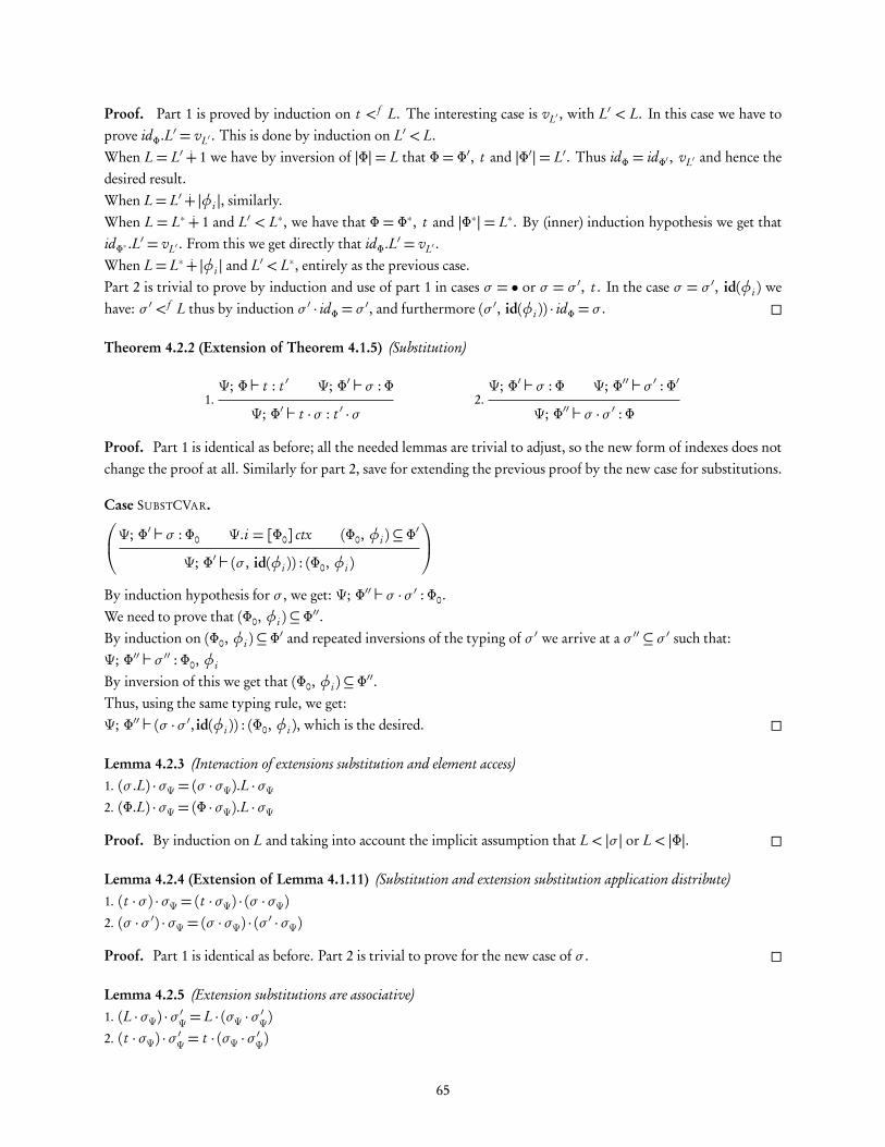
Proof. Part 1 is proved by induction on t < f L. The interesting case is vL′ , with L′ < L. In this case we have toprove idΦ.L′ = vL′ . This is done by induction on L′ < L.When L = L′õ 1 we have by inversion of |Φ| = L that Φ = Φ′, t and |Φ′| = L′. Thus idΦ = idΦ′ , vL′ and hence thedesired result.When L= L′õ |φi |, similarly.When L = L∗ õ 1 and L′ < L∗, we have that Φ = Φ∗, t and |Φ∗| = L∗. By (inner) induction hypothesis we get thatidΦ∗ .L

′ = vL′ . From this we get directly that idΦ.L′ = vL′ .When L= L∗õ |φi | and L′ < L∗, entirely as the previous case.Part 2 is trivial to prove by induction and use of part 1 in cases σ = • or σ = σ ′, t . In the case σ = σ ′, id(φi ) wehave: σ ′ < f L thus by induction σ ′ · idΦ = σ ′, and furthermore (σ ′, id(φi )) · idΦ = σ . �

Theorem 4.2.2 (Extension of Theorem 4.1.5) (Substitution)

1.Ψ; Φ ` t : t ′ Ψ; Φ′ ` σ : Φ

Ψ; Φ′ ` t ·σ : t ′ ·σ2.Ψ; Φ′ ` σ : Φ Ψ; Φ′′ ` σ ′ : Φ′

Ψ; Φ′′ ` σ ·σ ′ : Φ

Proof. Part 1 is identical as before; all the needed lemmas are trivial to adjust, so the new form of indexes does notchange the proof at all. Similarly for part 2, save for extending the previous proof by the new case for substitutions.

Case SUBSTCVAR.

Ψ; Φ′ ` σ : Φ0 Ψ.i = [Φ0] ctx (Φ0, φi )⊆ Φ′

Ψ; Φ′ ` (σ , id(φi )) : (Φ0, φi )

By induction hypothesis for σ , we get: Ψ; Φ′′ ` σ ·σ ′ : Φ0.We need to prove that (Φ0, φi )⊆ Φ′′.By induction on (Φ0, φi )⊆ Φ′ and repeated inversions of the typing of σ ′ we arrive at a σ ′′ ⊆ σ ′ such that:Ψ; Φ′′ ` σ ′′ : Φ0, φi

By inversion of this we get that (Φ0, φi )⊆ Φ′′.Thus, using the same typing rule, we get:Ψ; Φ′′ ` (σ ·σ ′, id(φi )) : (Φ0, φi ), which is the desired. �

Lemma 4.2.3 (Interaction of extensions substitution and element access)1. (σ .L) ·σΨ = (σ ·σΨ).L ·σΨ2. (Φ.L) ·σΨ = (Φ ·σΨ).L ·σΨ

Proof. By induction on L and taking into account the implicit assumption that L< |σ | or L< |Φ|. �

Lemma 4.2.4 (Extension of Lemma 4.1.11) (Substitution and extension substitution application distribute)1. (t ·σ) ·σΨ = (t ·σΨ) · (σ ·σΨ)2. (σ ·σ ′) ·σΨ = (σ ·σΨ) · (σ ′ ·σΨ)

Proof. Part 1 is identical as before. Part 2 is trivial to prove for the new case of σ . �

Lemma 4.2.5 (Extension substitutions are associative)1. (L ·σΨ) ·σ ′Ψ = L · (σΨ ·σ ′Ψ)2. (t ·σΨ) ·σ ′Ψ = t · (σΨ ·σ ′Ψ)

65

3. (Φ ·σΨ) ·σ ′Ψ =Φ · (σΨ ·σ′Ψ)

4. (σ ·σΨ) ·σ ′Ψ = σ · (σΨ ·σ′Ψ)

5. (T ·σΨ) ·σ ′Ψ = T · (σΨ ·σ ′Ψ)6. (K ·σΨ) ·σ ′Ψ =K · (σΨ ·σ ′Ψ)7. (Ψ ·σΨ) ·σ ′Ψ =Ψ · (σΨ ·σ

′Ψ)

Proof.

Part 1 By induction on L. The interesting case is L= L′õφi . In that case we have:

(L ·σΨ) ·σ′Ψ = (L

′ ·σΨ) ·σ′Ψõ |Φ

′| ·σ ′Ψ (assuming σΨ.i = [Φ]Φ′)

= (L′ ·σΨ) ·σ′Ψõ |Φ

′ ·σ ′Ψ|

= L′ · (σΨ ·σ′Ψ)õ |Φ

′ ·σ ′Ψ| (by induction hypothesis)

This is the desired, since (σΨ ·σ ′Ψ).i = [Φ ·σΨ]Φ′ ·σ ′Ψ.

Part 2 By induction on t . The interesting case is t =Xi/σ . The left-hand-side is then equal to:

(σΨ.i · (σ ·σΨ)) ·σ′Ψ = (t · (σ ·σΨ)) ·σ

′Ψ (assuming σΨ.i = [Φ] t )

= (t ·σ ′Ψ) · ((σ ·σΨ) ·σ′Ψ) (through Lemma 4.2.4)

= (t ·σ ′Ψ) · (σ · (σΨ ·σ′Ψ)) (through part 4)

The right-hand side is written as:

(Xi/σ) · (σΨ ·σ′Ψ) = ((σΨ ·σ

′Ψ).i) · (σ · (σΨ ·σ

′Ψ))

= ((σΨ.i) ·σ ′Ψ) · (σ · (σΨ ·σ′Ψ))

= ([Φ ·σ ′Ψ] (t ·σ′Ψ)) · (σ · (σΨ ·σ

′Ψ))

= (t ·σ ′Ψ) · (σ · (σΨ ·σ′Ψ))

Part 3 By induction on Φ. When Φ = Φ, φi and assuming σΨ.i = [Φ]Φ′ we have that the left-hand side is equalto:

(Φ ·σΨ) ·σ′Ψ, Φ′ ·σ ′Ψ =Φ · (σΨ ·σ

′Ψ), Φ

′ ·σ ′Ψ (by induction hypothesis)

Also, we have that (σΨ ·σ ′Ψ).i = [Φ ·σ′Ψ]Φ

′ ·σ ′Ψ3.

The right-hand-side is also equal to Φ · (σΨ ·σ ′Ψ), Φ′ ·σ ′Ψ.

Rest Similarly as above. �

Theorem 4.2.6 (Extension of Theorem 4.1.13) (Extension substitution application)

3. Typing will require that Φ ·σ ′Ψ =Φ · (σΨ ·σ′Ψ)

66

1.Ψ; Φ ` t : t ′ Ψ′ ` σΨ :Ψ

Ψ′; Φ ·σΨ ` t ·σΨ : t ′ ·σΨ2.Ψ; Φ ` σ : Φ′ Ψ′ ` σΨ :Ψ

Ψ′; Φ ·σΨ ` σ ·σΨ : Φ′ ·σΨ3.Ψ ` Φwf Ψ′ ` σΨ :Ψ

Ψ′ ` Φ ·σΨ wf

4.Ψ ` T : K Ψ′ ` σΨ :Ψ

Ψ′ ` T ·σΨ : K ·σΨ5.Ψ′ ` σΨ :Ψ Ψ′′ ` σ ′Ψ :Ψ′

Ψ′′ ` σΨ ·σ′Ψ :Ψ

Proof. We extend our previous proof as follows.

Case VAR.

Φ.L= t

Ψ; Φ ` vL : t

We have (Φ · σΨ).(L · σΨ) = (Φ.L) · σΨ = t · σΨ from Lemma 4.2.3. Thus using the same rule for vL·σΨ we get thedesired result.

Case SUBSTCVAR.

Ψ; Φ ` σ : Φ′ Ψ.i = [Φ′] ctx Φ′, φi ⊆ Φ

Ψ; Φ ` (σ , id(φi )) : (Φ′, φi )

In this case we need to prove that Ψ′; Φ ·σΨ ` (σ ·σΨ, idσΨ.i ) : (Φ′ ·σΨ, σΨ.i).

By induction hypothesis for σ we get that Ψ′; Φ ·σΨ ` σ ·σΨ : Φ′ ·σΨ.Also, we have that Ψ′ ` σΨ.i :Ψ.i ·σΨ.Since Ψ.i = [Φ′] ctx this can be rewritten as: Ψ′ ` σΨ.i : [Φ′ ·σΨ] ctx.By typing inversion get σΨ.i = [Φ′ ·σΨ]Φ′′ for some Φ′′ and:Ψ′ ` [Φ′ ·σΨ]Φ′′ : [Φ′ ·σΨ] ctx.Now proceed by induction on Φ′′ to prove thatΨ′; Φ ·σΨ ` (σ ·σΨ, idσΨ.i ) : (Φ

′ ·σΨ, σΨ.i).When Φ′′ = •, trivial.When Φ′′ = Φ′′′, t , have Ψ′; Φ · σΨ ` σ · σΨ, id[Φ′·σΨ]Φ′′′ : (Φ′ · σΨ, Φ′′′) by induction hypothesis. We can appendv|Φ′·σΨ|õ|Φ′′′| to this substitution and get the desired, because (|Φ′ ·σΨ|, |Φ′′′|) < |Φ ·σΨ|. This is because (Φ′, φi ) ⊆ Φthus (Φ′ ·σΨ, Φ′′′, t )⊆ Φ and (|Φ′ ·σΨ|õ |Φ′′′|õ 1)≤ |Φ|.When Φ′′ = Φ′′′, φ j , have Ψ′; Φ · σΨ ` σ · σΨ, id[Φ′·σΨ]Φ′′′ : (Φ′ · σΨ, Φ′′′). Now we have that Φ′, φi ⊆ Φ, whichalso means that (Φ′ · σΨ, Φ′′′, φ j ) ⊆ Φ · σΨ. Thus we can apply the typing rule for id(φ j ) to get that Ψ′; Φ · σΨ `σ ·σΨ, id[Φ′·σΨ]Φ′′′ , id(φ j ) : (Φ

′ ·σΨ, Φ′′′, φ j ), which is the desired.

Case CTXCVAR.

Ψ ` Φwf Ψ.i = [Φ] ctx

Ψ ` (Φ, φi )wf

By induction hypothesis we get Ψ′ ` Φ ·σΨ wf.Also, we have that Ψ′ ` σΨ.i :Ψ.i ·σΨ.Since Ψ.i = [Φ] ctx the above can be rewritten as Ψ′ ` σΨ.i : [Φ ·σΨ] ctx.By inversion of typing get that σΨ.i = [Φ ·σΨ]Φ′ and that Ψ′ ` Φ ·σΨ, Φ′ wf. This is exactly the desired result.

67

Case EXTCTXINST.

Ψ ` Φ, Φ′ wf

Ψ ` [Φ]Φ′ : [Φ] ctx

By use of part 3 we get Ψ′ ` Φ ·σΨ, Φ′ ·σΨ wf.Thus by the same typing rule we get exactly the desired.

Case EXTSVAR.

Ψ′ ` σΨ :Ψ Ψ′ ` T : K ·σΨΨ′ ` (σΨ, T ) : (Ψ, K)

By induction hypothesis we get Ψ′′ ` σΨ ·σ ′Ψ :Ψ.By use of part 4 we get Ψ′′ ` T ·σ ′Ψ : (K ·σΨ) ·σ ′Ψ.This is equal to K · (σΨ ·σ ′Ψ) by use of Lemma 4.2.5. Thus we get the desired result by applying the same typing rule.�

4.3 Constant schemata in signatures

The λHOL logic as presented so far does not allow for polymorphism over kinds. For example, it does not supportlists List α : Type of an arbitrary α : Type kind, or types for its associated constructor objects. Similarly, in orderto define the elimination principle for natural numbers, we need to provide one constant in the signature for eachindividual return kind that we use, with the following form:

elimNatK : K→ (Nat→K→K)→ (Nat→K)

Another similar case is the proof of symmetricity for equality given in Section 3.2, which needs to be parametric overthe kind of the involved terms. One way to solve this issue would be to include the PTS rule (Type′,Type,Type) inthe logic; but it is well known that this leads to inconsistency because of Girard’s paradox [Girard, 1972, Coquand,1986, Hurkens, 1995]. This in turn can be solved by supporting a predicative hierarchy of Type universes. We willconsider a different alternative instead: viewing the signatureΣ as a list of constant schemata instead of a (potentiallyinfinite) list of constants. Each schema expects a number of parameters, just as elimNat above needs the return kindK as a parameter; every instantiation of the schema can then be viewed as a different constant. Therefore this changedoes not affect the consistency of the system, as we can still view the signature of constant schemata as a signatureof constants.

This description of constant schemas corresponds exactly to the way that we have defined and used meta-variables above. We can see the context that a meta-variable depends on as a context of parameters and the sub-stitution required when using the meta-variable as the instantiation of those parameters. Therefore, we can supportconstant schematas by changing the signature Σ to be a context of meta-variables instead of a context of variables.We give the new syntax and typing rules for Σ in Figure 4.12. We give an example of using constant schematafor the definition of polymorphic lists in Figure 4.13, where we also provide constants for primitive recursion andinduction over lists. We use named variables for presentation purposes. We specify the substitutions used togetherwith the constant schemata explicitly; in the future we will omit these substitutions as they are usually trivial toinfer from context. Our version of λHOL supports inductive definitions of kinds and propositions that generate asimilar list of constants.

68

Syntax:

(Signature) Σ ::= • | Σ, c : [Φ] t(Logical terms) t ::= c/σ | · · ·

`Σwf

` •wfSIGEMPTY

`Σwf •; • `Σ [Φ] t : [Φ] s (c : _) 6∈Σ`Σ, c : [Φ] t wf

SIGCONST

Φ `Σ t : t ′

the rule CONSTANT is replaced by:

c : [Φ′] t ′ ∈Σ Ψ; Φ ` σ : Φ′

Ψ; Φ `Σ c/σ : t ′ ·σCONSTSCHEMA

Figure 4.12: Extension to λHOL with constant-schema-based signatures: Syntax and typing

It is trivial to adapt the metatheory lemmas we have proved so far in order account for this change. Intuitively,we can view the variable-based Σ context as a special variable context ΦΣ that is always prepended to the actualΦ context at hand; the metavariable-based Σ is a similar special metavariable context ΨΣ. The adaptation neededis therefore exactly equivalent to moving from the CONSTANT rule that corresponds to the VAR rule for using avariable out of a Φ context, to the CONSTSCHEMA rule corresponding to the METAVAR rule for using a metavariableout of Ψ. Since we have proved that all our lemmas still hold in the presence of the METAVAR rule, they will alsohold in the presence of CONSTSCHEMA. With the formal description of constant schemata in place, we can makethe reason why the consistency of the logic is not influenced precise: extension terms and their types, where theextra dependence on parameters is recorded, are not internalized within the logic – they do not become part of thenormal logical terms. Thus [Type]Type is not a Type, therefore Type is not predicative and Girard’s paradox cannotbe encoded.

4.4 Named extension variables

We have only considered the case where extension variables Xi and φi are free. This is enough in order to makeuse of extension variables in λHOL, as the logic itself does not include constructs that bind these kinds of variables.Our computational language, on the other hand, will need to be able to bind extension variables. We thus need toextend λHOL so that we can use such bound extension variables in further logical terms.

In the interests of avoiding needlessly complicating our presentation, we will use named extension variablesinstead in our description of the computational language, which follows in Chapter 6. As mentioned earlier inSection 4.1, our original choice of using hybrid deBruijn variables for extension variables is not as integral as it isfor normal variables; we made it having future extensions in mind (such as meta-N-variables) and in order to be asclose as possible to the variable representation we use in our implementation. We will thus not discuss the extensionwith bound extension variables further, as using named extension variables masks the distinction between free andbound variables. The extension closely follows the definitions and proofs for normal variables and their associatedfreshening and binding operations, generalizing them to the case where we bind multiple extension variables at

69

List : [α : Type]Typenil : [α : Type]List/(α)cons : [α : Type]α→ List/(α)→ List/(α)elimList : [α : Type, T : Type]

T → (α→ List/(α)→ T → T )→ (List/(α)→ T )elimListNil : [α : Type, T : Type]

∀ fn : T .∀ fc : α→ List/α→ T → T .elimList/(α, T ) fn fc nil/α= fn

elimListCons : [α : Type, T : Type]∀ fn : T .∀ fc : α→ List/α→ T → T .∀t : α.∀l : List/α.elimList/(α, T ) fn fc (cons/α t l ) =

fc t l (elimList/(α, T ) fn fc l )indList : [α : Type, P : List/α→ Type]

P nil/α→ (∀t : α.∀l : α.P l → P (cons/α t l ))→∀l : List/α.P l

Figure 4.13: Definition of polymorphic lists in λHOL through constant schemata

(Logical terms) t ::= X /σ(Parametric deBruijn levels) L ::= 0 | Lõ 1 | Lõ |φ|

(Contexts) Φ ::= · · · | Φ, φ(Substitutions) σ ::= · · · | σ , id(φ)

(Extension variables) V ::= X | φ(Extension terms) T ::= [Φ] t | [Φ]Φ′(Extension types) K ::= [Φ] t | [Φ] ctx

(Extension contexts) Ψ ::= • | Ψ, V : K(Extension substitutions) σΨ ::= • | σΨ, T /V

Figure 4.14: λHOL with named extension variables: Syntax

once. The interested reader can find the full details of this extension in our published Technical Report [Stampoulisand Shao, 2012b].

We show the new syntax that uses named extension variables in Figure 4.14 and the new typing rules in Fig-ure 4.15. The main change is that we have included variable names in extension contexts and extension substitutions.We use V for extension variables when it is not known whether they are metavariables X or context variables φ.Furthermore, instead of using integers to index into contexts and substitutions we use names. The connection withthe formulation where extension variables are deBruijn indices is direct. Last, we will sometimes use the standardsubstitution notation T ′[T /V ] to denote the operation T ′ · (idΨ, T /V ), when the exact Ψ context needed is easilyinferrable from the context.

70

Ψ `Σ Φwf

Ψ ` Φwf Ψ.φ= [Φ] ctx

Ψ ` (Φ, φ)wfCTXCVAR

Ψ; Φ ` σ : Φ′

Ψ; Φ ` σ : Φ′ Ψ.φ= [Φ′] ctx (Φ′, φ)⊆ ΦΨ; Φ ` (σ , id(φ)) : (Φ′, φ)

SUBSTCVAR

Ψ; Φ ` t : t ′

Ψ.X = T T = [Φ′] t ′ Ψ; Φ ` σ : Φ′

Ψ; Φ `X /σ : t ′ ·σMETAVAR

`Ψwf

` •wfEXTCEMPTY

`Ψwf Ψ ` Φwf

` (Ψ, φ : [Φ] ctx)wfEXTCMETA

`Ψwf Ψ ` [Φ] t : [Φ] s

` (Ψ, X : [Φ] t )wfEXTCCTX

Ψ ` σΨ :Ψ′

Ψ ` • : •EXTSEMPTY

Ψ ` σΨ :Ψ′ Ψ ` T : K ·σΨΨ ` (σΨ, T /V ) : (Ψ′, V : K)

EXTSVAR

Figure 4.15: λHOL with named extension variables: Typing

71

Chapter 5

The logic λHOL: Pattern matching

Having presented λHOL with extension variables, we are ready to proceed to the main operation through whichλHOL terms are manipulated in VeriML: pattern matching. We will first describe the procedure and metatheoreticproofs for matching a scrutinee against a pattern in Section 5.1. In Section 5.2, we will present an approach thatenables us to use the same pattern matching procedure when the scrutinee is not closed with respect to extensionvariables.

5.1 Pattern matching

In Section 2.3 we noted the central importance that pattern matching constructs have in VeriML. We presented twoconstructs: one for matching over contextual terms and one for matching over contexts. Having seen the detailsof extension terms in the previous chapter, it is now clear that these two constructs are in fact a single constructfor pattern matching over extension terms T . In this section we will give the details of what patterns are, howunification of a pattern against a term works and prove the main metatheoretic result about this procedure.

Informally we can say that a pattern is the ‘skeleton’ of a term, where some parts are specified and some partsare missing. We name each missing subterm using unification variables. An example is the following pattern for aproposition, where we denote unification variables by prefixing them with a question mark:

?P ∧ (∀x : Nat.?Q)

A pattern matches a term when we can find a substitution for the missing parts so that the pattern is rendered equalto the given term. For example, the above pattern matches the term (∀x : Nat.x + x ≥ x)∧ (∀x : Nat .x ≥ 0) usingthe substitution:

?P 7→ (∀x : Nat.x + x ≥ x), ?Q 7→ x ≥ 0

As the above example suggests, unification variables can be used in patterns under the binding constructs of theλHOL logic. Because of this, if we view unification variables as typed variables, their type includes the informationabout the variables context of the missing subterm, in addition to its type. It is therefore evident that unificationvariables are a special kind of meta-variables; and that we can view the substitution returned from pattern matchingas being composed from contextual terms to be substituted for these (unification) meta-variables. The situationfor matching contexts against patterns that include context unification variables is similar. Therefore we can viewpatterns as a special kind of extension terms where the extension variables used are viewed as unification variables.We will place further restrictions on what terms are allowed as patterns, resulting in a new typing judgement that

72

we will denote as Ψ p T : K . Based on these, we can formulate pattern matching for λHOL as follows. Assuming apattern TP and an extension term T (the scrutinee) with the following typing:

Ψu p TP : K and • ` T : K

where the extension context Ψu describes the unification variables used in TP , pattern matching is a procedurewhich decides whether a substitution σΨ exists so that:

• ` σΨ :Ψu and TP ·σΨ = T

We will proceed as follows.

1. First, we will define the typing judgement for patternsΨ p T : K . This will be mostly identical to the normaltyping for terms, save for certain restrictions so that pattern matching is decidable and deterministic.

2. Then, we will define an operation to extract the relevant variables out of typing derivations; it will work byisolating the partial context that gets used in a given derivation. This is useful for two reasons: first, to ensurethat all the defined unification variables get used in a pattern; otherwise, pattern matching would not bedeterministic as unused variables could be instantiated with any arbitrary term. Second, isolating the partialcontext is crucial in stating the induction principle needed for the pattern matching theorem that we willprove.

3. Using this operation, we will define an even more restrictive typing judgement for patterns, which requiresall unification variables defined to be relevant, ruling out in this way variables that are not used. A sketch ofits formal definition is as follows:

Ψ, Ψu p TP : K relevant�

Ψ, Ψu p TP : K�

= · · · ,Ψu

Ψ ∗p Ψu > TP : K

Let us explain this rule briefly. First, Ψ represents the normal extension variables whereas Ψu represents thenewly-defined unification variables. The judgement Ψ ∗

p Ψu > TP : K is understood as: “in extension contextΨ, the introduction of the unification variables Ψu renders TP a valid pattern of extension type K”. Thesecond premise of this rule uses the operation that extracts relevant variables out of a derivation in order tomake sure that all unification variables are relevant. We will prove a substitution theorem for this rule, withthe following formal statement:

Ψ ∗p Ψu > TP : K Ψ′ ` σΨ :Ψ

Ψ′ ∗p Ψu ·σΨ > TP ·σΨ : K ·σΨSUBSTITUTION LEMMA

This theorem extends the extension substitution theorem 4.2.6 so as to apply to the case of patterns as well.

4. Based on these, we will prove the fact that pattern matching is decidable and deterministic. We will carry outthe proof in a constructive manner; its computational counterpart will be the pattern matching algorithmthat we will use. Therefore the pattern matching algorithm will be sound and complete directly by construc-tion. The algorithm thus produces a substitution σΨ of instantiations to the unification variables making thepattern and the scrutinee match, when one such substitution exists; or fails, when there is no such substitu-tion. We write TP ∼ T = σΨ for an execution of this algorithm between the pattern TP and the scrutinee

73

T , when it results in a substitution σΨ. Formally, the statements of the related theorems we will prove are asfollows.

• ∗p Ψu > TP : K • ` T : K

∃≤1σΨ.( • ` σΨ :Ψu TP ·σΨ = T )

PATTERN MATCHING

DETERMINISM AND DECIDABILITY

• ∗p Ψu > TP : K • ` T : K TP ∼ T = σΨ

• ` σΨ :Ψu TP ·σΨ = T

PATTERN MATCHING

ALGORITHM SOUNDNESS

• ∗p Ψu > TP : K • ` T : K

∃σΨ.( • ` σΨ :Ψu TP ·σΨ = T )

TP ∼ T = σΨ

PATTERN MATCHING

ALGORITHM COMPLETENESS

Pattern typing

In Figures 5.1 and 5.2 we give the details of pattern typing. The typing judgements use the extension contextΨ, Ψu ,composed from the normal extension variable contextΨ and the context of unification variablesΨu . We will definethe “actual” pattern matching process only between a ‘closed’ pattern and a closed extension term, so the case willbe that Ψ = •, as presented above. Yet being able to mention existing variables from an Ψ context will be usefulin order to describe patterns that exactly match a yet-unspecified term. It is thus understood that even if a patterndepends on extension variables in a non-empty Ψ context, those will have been substituted by concrete terms bythe time that the “actual” pattern matching happens.

The two kinds of variables are handled differently in the pattern typing rules themselves. For example, therule for using an exact context variable PCTXCVAREXACT is different than the rule for using a unification contextvariable PCTXCVARUNIFY. The difference is subtle: the latter rule does not allow existing unification variablesto inform the well-formedness of the Φ context; in other words, a unification context variable cannot be used ina pattern after another unification context variable has already been used. Consider the pattern φ0, φ1, whereφ1 : [φ0] ctx. Any non-empty context could be matched against this pattern, yet the exact point of the split betweenwhich variables belong to the φ0 context and which to φ1 is completely arbitrary. This would destroy determinacyof pattern matching thus this form is disallowed using this rule.

Metavariables typing in patterns is similarly governed by two rules: PMETAVAREXACT and PMETAVARUNIF. Theformer is the standard typing rule for metavariables save for a sort restriction which we will comment on shortly.The latter is the rule for using a unification variable. The main restriction that it has is that the substitution σ usedmust be the identity substitution – or more accurately, the identity substitution for a prefix of the current context.If arbitrary substitutions were allowed, matching a pattern Xi/σ against a term t would require finding an inversesubstitution σ−1 and using t · σ−1 as the instantiation for Xi , so that t · σ−1 · σ = t . This destroys determinacyof pattern matching, as multiple inverse substitutions might be possible; but it also destroys decidability if furtherunification variables are allowed inside σ , as the problem becomes equivalent to higher-order unification, whichis undecidable [Dowek, 2001]. Prefixes of the identity substitution for the current context can be used to matchagainst scrutinees that only mention specific variables. For example we can use a pattern like Xi/• in order to matchagainst closed terms.

Last, many pattern typing rules impose a sort restriction. The reason is that we want to disallow pattern match-ing against proof objects, so as to render the exact structure of proof objects computationally irrelevant. We cannot

74

Ψ p Ψu wf

Ψ p •wfUVAREMPTY

Ψ p Ψu wf Ψ, Ψu p [Φ] t : [Φ] s

Ψ p (Ψu , [Φ] t )wfUVARMETA

Ψ p Ψu wf Ψ, Ψu p Φwf

Ψ p (Ψu , [Φ] ctx)wfUVARCTX

Ψ, Ψu p T : K

Ψ, Ψu ; Φ p t : t ′ Ψ, Ψu ; Φ ` t ′ : s

Ψ, Ψu p [Φ] t : [Φ] t ′PEXTCTXTERM

Ψ, Ψu p Φ, Φ′ wf

Ψ, Ψu p [Φ]Φ′ : [Φ] ctx

PEXTCTXINST

Ψ, Ψu p Φwf

Ψ, Ψu p •wfPCTXEXPTY

Ψ, Ψu p Φwf Ψ, Ψu ; Φ p t : s

Ψ, Ψu p (Φ, t )wfPCTXVAR

Ψ, Ψu p Φwf i < |Ψ| (Ψ, Ψu ).i = [Φ] ctx

Ψ, Ψu p (Φ, φi )wfPCTXCVAREXACT

Ψ p Φwf i ≥ |Ψ| (Ψ, Ψu ).i = [Φ] ctx

Ψ, Ψu p (Φ, φi )wfPCTXCVARUNIF

Ψ, Ψu ; Φ p σ : Φ′

Ψ, Ψu ; Φ p • : •PSUBSTEMPTY

Ψ, Ψu ; Φ p σ : Φ′ Ψ, Ψu ; Φ p t : t ′ ·σ

Ψ, Ψu ; Φ p (σ , t ) : (Φ′, t ′)PSUBSTVAR

Ψ, Ψu ; Φ p σ : Φ′ (Ψ, Ψu ).i = [Φ′] ctx Φ′, φi ⊆ Φ

Ψ, Ψu ; Φ p (σ , id(φi )) : (Φ′, φi )

PSUBSTCVAR

Figure 5.1: Pattern typing for λHOL

75

Ψ, Ψu ; Φ p t : t ′

c : t ∈Σ •; • ` t : s s 6= Prop

Ψ, Ψu ; Φ p c : tPCONSTANT

Φ.L= t Ψ, Ψu ; Φ ` t : s s 6= Prop

Ψ, Ψu ; Φ p vL : tPVAR

(s , s ′) ∈AΨ, Ψu ; Φ p s : s ′

PSORTΨ, Ψu ; Φ p t1 : s Ψ, Ψu ; Φ, t1 p dt2e|Φ| : s ′ (s , s ′, s ′′) ∈R

Ψ, Ψu ; Φ p Π(t1).t2 : s ′′PΠTYPE

Ψ, Ψu ; Φ p t1 : s Ψ, Ψu ; Φ, t1 p dt2e|Φ| : t ′ Ψ, Ψu ; Φ p Π(t1).�

t ′�

|Φ|õ1 : s ′ s ′ 6= Prop

Ψ, Ψu ; Φ p λ(t1).t2 :Π(t1).�

t ′�

|Φ|õ1

PΠINTRO

Ψ, Ψu ; Φ p t1 :Π(t ).t ′ Ψ, Ψu ; Φ p t2 : t Ψ, Ψu ; Φ p Π(t ).t′ : s ′ s ′ 6= Prop

Ψ, Ψu ; Φ p t1 t2 :�

t ′�

|Φ| · (idΦ, t2)PΠELIM

Ψ, Ψu ; Φ p t1 : t Ψ, Ψu ; Φ p t2 : t Ψ, Ψu ; Φ p t : Type

Ψ, Ψu ; Φ p t1 = t2 : PropPEQTYPE

(Ψ, Ψu ).i = TT = [Φ′] t ′ i < |Ψ| Ψ, Ψu ; Φ p σ : Φ′ Ψ, Ψu ` t ′ : s ′ s 6= Prop

Ψ, Ψu ; Φ p Xi/σ : t ′ ·σPMETAVAREXACT

(Ψ, Ψu ).i = T T = [Φ′] t ′

i ≥ |Ψ| Ψ, Ψu ; Φ p σ : Φ′ Φ′ ⊆ Φ σ = idΦ′ Ψ, Ψu ` t ′ : s ′ s 6= Prop

Ψ, Ψu ; Φ p Xi/σ : t ′ ·σPMETAVARUNIF

Figure 5.2: Pattern typing for λHOL (continued)

76

Assuming Ψ `Ψu wf:

T =Vi

Xi = [Φ]Xi/idΦ when (Ψ, Ψu ).i = [Φ] t ′

φi = [Φ]φi when (Ψ, Ψu ).i = [Φ] ctx

idΨu

id• = •idΨ′u , K = idΨ′u , V|Ψ|+|Ψ′u |

Ψu ·σΨ• ·σΨ = •(Ψ′u , K) ·σΨ = Ψ′u ·σΨ, K · (σΨ, idΨ′u )

Figure 5.3: Syntactic operations for unification contexts

thus look inside proof objects: we are only interested in the existence of a proof object and not in its specific details.This will enable us to erase proof objects prior to evaluation of VeriML programs. By inspection of the rules it isevident that Prop-sorted terms are not well-typed as patterns; these terms are exactly the proof objects. The onlyProp-sorted pattern that is allowed is the unification variable case, which we can understand as a wildcard rule formatching any proof object of a specific proposition.

We will need some metatheoretic facts about pattern typing: first, the fact that pattern typing implies normaltyping; and second, the equivalent of the extension substitution theorem 4.2.6 for patterns. We will first need twodefinitions that lift identity substitutions and extension substitution application to unification contexts Ψu typedin a context Ψ, given in Figure 5.3. In the same figure we give an operation to include extension variables Vi asextension terms, by expanding them to the existing forms such as [Φ]Vi/idΦ and [Φ]Vi . We remind the reader thatVi stands for either kind of an extension variable, that is, either for a meta-variable Xi or for a context variable φi .

Lemma 5.1.1 (Pattern typing implies normal typing)

1.Ψ p Ψu wf

`Ψ, Ψu wf2.Ψ, Ψu p T : K

Ψ, Ψu ` T : K3.Ψ, Ψu p Φwf

Ψ, Ψu ` Φwf

4.Ψ, Ψu p σ : Φ

Ψ, Ψu ` σ : Φ5.Ψ, Ψu ; Φ p t : t ′

Ψ, Ψu ; Φ ` t : t ′

Proof. Trivial by induction on the typing derivations, as every pattern typing rule is a restriction of an existingnormal typing rule. �

Theorem 5.1.2 (Extension substitution application preserves pattern typing)

77

Assuming Ψ′ ` σΨ :Ψ and σ ′Ψ = σΨ, idΨu,

1.Ψ, Ψu ; Φ p t : t ′

Ψ′, Ψu ·σΨ; Φ ·σ ′Ψ p t ·σ ′Ψ : t ′ ·σ ′Ψ2.

Ψ, Ψu ; Φ p σ : Φ′

Ψ′, Ψu ·σΨ; Φ ·σ ′Ψ p σ ·σ′Ψ : Φ′ ·σ ′Ψ

3.Ψ, Ψu p Φwf

Ψ′, Ψu ·σΨ p Φ ·σ′Ψ wf

4.Ψ, Ψu p T : K

Ψ′, Ψu ·σΨ p T ·σ ′Ψ : K ·σ ′Ψ5.Ψ p Ψu wf

Ψ p Ψu ·σΨ wf

Proof. In most cases proceed similarly as before. The cases that deserve special mention are the ones that placeextra restrictions compared to normal typing.

Case PCTXCVARUNIF.

Ψ p Φwf i ≥ |Ψ| (Ψ, Ψu ).i = [Φ] ctx

Ψ, Ψu p (Φ, φi )wf

We need to prove that Ψ′, Ψu ·σΨ p Φ ·σ ′Ψ, φi ·σ ′Ψ wf.We have that φi ·σ ′Ψ =φi−|Ψ|+|Ψ′|.By induction hypothesis for Φ, with Ψu = •, we get:Ψ p Φ ·σΨ wf from which Ψ p Φ ·σ ′Ψ wf directly follows.We have i − |Ψ|+ |Ψ′| ≥ |Ψ′| because of i ≥ |Ψ|.Last, we have that (Ψ′, Ψu ·σΨ).(i − |Ψ|+ |Ψ′|) = [Φ ·σ ′Ψ] ctx.Thus using the same rule PCTXCVARUNIF we arrive at the desired.

Case PMETAVARUNIF.

(Ψ, Ψu ).i = T T = [Φ′] t ′ i ≥ |Ψ| Ψ, Ψu ; Φ p σ : Φ′ Φ′ ⊆ Φ σ = idΦ′

Ψ, Ψu ; Φ p Xi/σ : t ′ ·σ

Similar as above. Furthermore, we need to show that idΦ′ ·σ ′Ψ = idΦ′·σ ′Ψ , which follows trivially by induction on Φ′.

Case PVAR.

Φ.L= t Ψ, Ψu ; Φ ` t : s s 6= Prop

Ψ, Ψu ; Φ p vL : t

We give the proof for this rule as an example of accounting for the sort restriction; other rules are proved similarly.By induction hypothesis for t we get:Ψ′, Ψu ·σΨ; Φ ·σ ′Ψ ` t ·σ ′Ψ : s ·σ ′ΨBut s ·σ ′Ψ = s so the restriction s 6= Prop still holds. �

The statement of the above lemma might be surprising at first. One could expect it to hold for the general casewhere Ψ′ ` σΨ : (Ψ, Ψu ). This stronger statement is not true however, if we take into account the restrictionswe have placed: for example, substituting a unification variable for a proof object will result in a term that is notallowed as a pattern. The statement we have proved is in fact all we need, as we will use it only in cases where we aresubstituting the base Ψ context; the unification variables will only be substituted by new unification variables thatare well-typed in the resulting Ψ′ context. This becomes clearer if we consider a first sketch of the pattern typing

78

rule used in the computational language:

Ψ ` T : K Ψ p Ψu wf Ψ, Ψu p TP : K · · ·

Ψ · · · `match T with TP 7→ · · ·

Type-safety of the computational language critically depends on the fact that applying a substitution σΨ for thecurrent Ψ context yields expressions that are typable using the same typing rule. This fact is exactly what can beproved using the lemma as stated.

Relevant typing

We will now proceed to define the notion of relevant variables and partial contexts. We say that a variable is relevantfor a term if it is used either directly in the term or indirectly in its type. A partial context bΨ is a context whereonly the types for the relevant variables are specified; the others are left unspecified, denoted as ?. We will define anoperation relevant (Ψ; · · · ) for derivations that isolates the partial context required for the relevant variables of thejudgement. For example, considering the derivation resulting in:

φ0 : [] ctx, X1 : [φ0]Type, X2 : [φ0]X1, X3 : [φ0]X1 `X3 : [φ0]X1

the resulting partial context will be:

bΨ=φ0 : [] ctx, X1 : [φ0]Type, X2 : ?, X3 : [φ0]X1

where the variable X2 was unused in the derivation and is therefore left unspecified in the resulting partial context.The typing rule for patterns in the computational language will require that all unification variables are relevantin order to ensure determinacy as noted above. Non-relevant variables can be substituted by arbitrary terms, thuspattern-matching would have an infinite number of valid solutions if we allowed them. Thus a refined sketch of thepattern match typing rule is:

Ψ ` T : K Ψ p Ψu wf Ψ, Ψu p TP : K?, ?, · · · , ?,Ψu v relevant

�

Ψ, Ψu p TP : K�

· · ·

Ψ · · · `match T with TP 7→ · · ·

In this, the symbol v is used to mean that one partial context is less-specified than another one. Therefore, in thenew restriction placed by the typing rule, we require that all unification variables are used in a pattern but normalextension variables can either be used or unused. Because of this extra restriction, we will need to prove a lemmaregarding the interaction of relevancy with extension substitution application, so that the extension substitutionlemma needed for the computational language will still hold.

We present the syntax and typing for partial contexts in Figure 5.4; these are entirely identical to normal Ψcontexts save for the addition of the case of an unspecified element. We present several operations involving partialcontexts in Figure 5.5; we use these to define the operation of isolating the relevant variables of a judgement inFigures 5.6 and 5.7. The rules are mostly straightforward. For example, in the case of the rule METAVAR for usingmetavariables, the relevant variables are: the metavariable itself (by isolating just that variable from the context Ψthrough the Ψb@i operation); the relevant variables used for the substitution σ ; and the variables that are relevantfor well-typedness of the type of the metavariable [Φ′] t ′. The partial contexts so constructed are joined togetherthrough the Ψ ◦Ψ′ operation in order to get the overall result. This is equivalent to taking the union of the set ofrelevant variables in informal practice.

We are now ready to proceed to the metatheoretic proofs about isolating relevant variables.

79

bΨ ::= • | bΨ, K | bΨ, ?

` •wf

` bΨwf bΨ ` [Φ] t : [Φ] s

` (bΨ, [Φ] t )wf

` bΨwf bΨ ` Φwf

` (bΨ, [Φ] ctx)wf

` bΨwf

` (bΨ, ?)wf

Figure 5.4: Partial contexts (syntax and typing)

Fully unspecified context:unspecΨ = bΨ

unspec• = •unspecΨ, K = unspecΨ, ?

Partial context solely specified at i :Ψb@i = bΨ

(Ψ, K)b@i = unspecΨ, K when |Ψ|= i(Ψ, K)b@i = (Ψb@i), ? when |Ψ|> i

Joining two partial contexts:bΨ ◦ bΨ′ = bΨ′′

• ◦ • = •(bΨ, K) ◦ (bΨ′, K) = (bΨ ◦ bΨ′), K(bΨ, ?) ◦ (bΨ′, K) = (bΨ ◦ bΨ′), K(bΨ, K) ◦ (bΨ′, ?) = (bΨ ◦ bΨ′), K(bΨ, ?) ◦ (bΨ′, ?) = (bΨ ◦ bΨ′), ?

Context bΨ less specified than bΨ′:bΨv bΨ′

• v •(bΨ, K)v (bΨ′, K) ⇐ bΨv bΨ′

(bΨ, ?)v (bΨ′, K) ⇐ bΨv bΨ′

(bΨ, ?)v (bΨ′, ?) ⇐ bΨv bΨ′

Extension substitution application:(assuming Ψ ` bΨu wf)

bΨ ·σΨ• ·σΨ = •(bΨu , K) ·σΨ = bΨu ·σΨ, K · (σΨ, id

bΨu)

(bΨu , ?) ·σΨ = bΨu ·σΨ, ?

Figure 5.5: Partial contexts (syntactic operations)

80

relevant (Ψ ` T : K) = bΨ

relevant

Ψ; Φ ` t : t ′ Ψ; Φ ` t ′ : s

Ψ ` [Φ] t : [Φ] t ′

!

= relevant�

Ψ; Φ ` t : t ′�

relevant

Ψ ` Φ, Φ′ wf

Ψ ` [Φ]Φ′ : [Φ] ctx

!

= relevant�

Ψ ` Φ, Φ′ wf�

relevant�

Ψ ` Φwf�

= bΨ

relevant

Ψ ` •wf

!

= unspecΨ

relevant

Ψ ` Φwf Ψ; Φ ` t : s

Ψ ` (Φ, t )wf

!

= relevant (Ψ; Φ ` t : s)

relevant

Ψ ` Φwf (Ψ).i = [Φ] ctx

Ψ ` (Φ, φi )wf

!

= relevant�

Ψ ` Φwf�

◦ (Ψb@i)

relevant�

Ψ; Φ ` σ : Φ′�

= bΨ

relevant

Ψ; Φ ` • : •

!

= relevant�

Ψ ` Φwf�

relevant

Ψ; Φ ` σ : Φ′ Ψ; Φ ` t : t ′ ·σΨ; Φ ` (σ , t ) : (Φ′, t ′)

!

=

= relevant�

Ψ; Φ ` σ : Φ′�

◦ relevant�

Ψ; Φ ` t : t ′ ·σ�

relevant

Ψ; Φ ` σ : Φ′ Ψ.i = [Φ′] ctx Φ′, φi ⊆ ΦΨ; Φ ` (σ , id(φi )) : (Φ

′, φi )

!

= relevant�

Ψ; Φ ` σ : Φ′�

Figure 5.6: Relevant variables of λHOL derivations

81

relevant�

Ψ; Φ ` t : t ′�

= bΨ

relevant

c : t ∈ΣΨ; Φ ` c : t

!

= relevant�

Ψ ` Φwf�

relevant

Φ.L= t

Ψ; Φ ` vL : t

!

= relevant�

Ψ ` Φwf�

relevant

(s , s ′) ∈AΨ; Φ ` s : s ′

!

= relevant�

Ψ ` Φwf�

relevant

Ψ; Φ ` t1 : s Ψ; Φ, t1 ` dt2e|Φ| : s ′ (s , s ′, s ′′) ∈R

Ψ; Φ `Π(t1).t2 : s ′′

=

= relevant�

Ψ; Φ, t1 ` dt2e|Φ| : s ′�

relevant

Ψ; Φ ` t1 : s Ψ; Φ, t1 ` dt2e|Φ| : t ′ Ψ; Φ `Π(t1).�

t ′�

|Φ|õ1 : s ′

Ψ; Φ ` λ(t1).t2 :Π(t1).�

t ′�

|Φ|õ1

=

= relevant�

Ψ; Φ, t1 ` dt2e|Φ| : t ′�

relevant

Ψ; Φ ` t1 :Π(t ).t ′ Ψ; Φ ` t2 : t

Ψ; Φ ` t1 t2 :�

t ′�

|Φ| · (idΦ, t2)

=

= relevant�

Ψ; Φ ` t1 :Π(t ).t ′�

◦ relevant (Ψ; Φ ` t2 : t )

relevant

Ψ; Φ ` t1 : t Ψ; Φ ` t2 : t Ψ; Φ ` t : Type

Ψ; Φ ` t1 = t2 : Prop

!

=

= relevant (Ψ; Φ ` t1 : t ) ◦ relevant (Ψ; Φ ` t2 : t )

relevant

(Ψ).i = T T = [Φ′] t ′ Ψ; Φ ` σ : Φ′

Ψ; Φ `Xi/σ : t ′ ·σ

!

=

= relevant�

Ψ ` [Φ′] t ′ : [Φ′] s�

◦ relevant�

Ψ; Φ ` σ : Φ′�

◦ (Ψb@i)

Figure 5.7: Relevant variables of λHOL derivations (continued)

82

Lemma 5.1.3 (More specified contexts preserve judgements)Assuming bΨv bΨ′:

1.bΨ ` T : K

bΨ′ ` T : K2.bΨ ` Φwf

bΨ′ ` Φwf3.bΨ; Φ ` t : t ′

bΨ′; Φ ` t : t ′4.bΨ; Φ ` σ : Φ′

bΨ′; Φ ` σ : Φ′

Proof. Simple by structural induction on the judgements. The interesting cases are the ones mentioning extensionvariables, as for example when Φ = Φ′, φi , or t = Xi/σ . In both such cases, the typing rule has a side conditionrequiring that bΨ.i = T . Since bΨv bΨ′, we have that bΨ′.i = bΨ.i = T . �

Lemma 5.1.4 (Relevancy is decidable)

1.Ψ ` T : K

∃!bΨ.relevant (Ψ ` T : K) = bΨ2.

Ψ ` Φwf

∃!bΨ.relevant (Ψ ` Φwf) = bΨ3.

Ψ; Φ ` t : t ′

∃!bΨ.relevant�

Ψ; Φ ` t : t ′�

= bΨ

4.Ψ; Φ ` σ : Φ′

∃!bΨ.relevant�

Ψ; Φ ` σ : Φ′�

= bΨ

Proof. The relevancy judgements are defined by structural induction on the corresponding typing derivations. Itis crucial to take into account the fact that `Ψwf and Ψ ` Φwf are implicitly present in any typing derivation thatmentions such contexts; thus these derivations themselves, as well as their sub-derivations, are structurally includedin derivations like Ψ; Φ ` t : t ′. Furthermore, it is easy to see that all the partial context joins used are defined, as inall cases the joined contexts are less-specified versions of Ψ. This fact follows by induction on the derivation of theresult of the relevancy operation and by inspecting the base cases for the partial contexts returned. �

Lemma 5.1.5 (Relevancy soundness)

1.

Ψ ` T : Krelevant (Ψ ` T : K) = bΨ

bΨ ` T : K2.

Ψ ` Φwfrelevant (Ψ ` Φwf) = bΨ

bΨ ` Φwf

3.

Ψ; Φ ` t : t ′

relevant�

Ψ; Φ ` t : t ′�

= bΨ

bΨ; Φ ` t : t ′4.

Ψ; Φ ` σ : Φ′

relevant�

Ψ; Φ ` σ : Φ′�

= bΨ

bΨ; Φ ` σ : Φ′

Proof. By induction on the typing derivations. �

Theorem 5.1.6 (Interaction of relevancy and extension substitution)

83

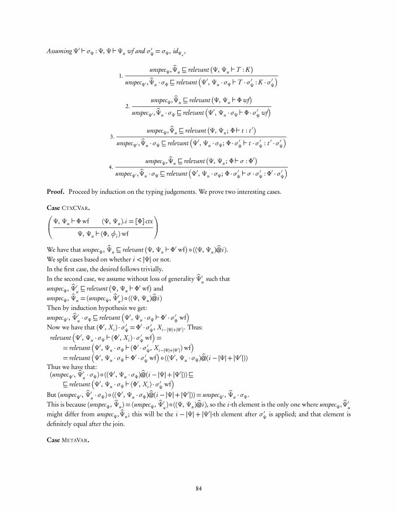
Assuming Ψ′ ` σΨ :Ψ, Ψ `Ψu wf and σ ′Ψ = σΨ, idΨu,

1.unspecΨ, bΨu v relevant

�

Ψ, Ψu ` T : K�

unspecΨ′ , bΨu ·σΨ v relevant�

Ψ′, Ψu ·σΨ ` T ·σ ′Ψ : K ·σ ′Ψ�


�

Ψ, Ψu ` Φwf�


Ψ′, Ψu ·σΨ ` Φ ·σ′Ψ wf

�


�

Ψ, Ψu ; Φ ` t : t ′�


Ψ′, Ψu ·σΨ; Φ ·σ ′Ψ ` t ·σ ′Ψ : t ′ ·σ ′Ψ�


�

Ψ, Ψu ; Φ ` σ : Φ′�


Ψ′, Ψu ·σΨ; Φ ·σ ′Ψ ` σ ·σ′Ψ : Φ′ ·σ ′Ψ

�

Proof. Proceed by induction on the typing judgements. We prove two interesting cases.

Case CTXCVAR.

Ψ, Ψu ` Φwf (Ψ, Ψu ).i = [Φ] ctx

Ψ, Ψu ` (Φ, φi )wf

We have that unspecΨ, bΨu v relevant�

Ψ, Ψu ` Φ′ wf�

◦ ((Ψ, Ψu )b@i).We split cases based on whether i < |Ψ| or not.In the first case, the desired follows trivially.In the second case, we assume without loss of generality bΨ′u such thatunspecΨ, bΨ′u v relevant

�

Ψ, Ψu ` Φ′ wf�

andunspecΨ, bΨu = (unspecΨ, bΨ′u ) ◦ ((Ψ, Ψu )b@i)Then by induction hypothesis we get:unspecΨ′ , bΨ

′u ·σΨ v relevant

�

Ψ′, Ψu ·σΨ ` Φ′ ·σ ′Ψ wf�

Now we have that (Φ′, Xi ) ·σ ′Ψ =Φ′ ·σ ′Ψ, Xi−|Ψ|+|Ψ′|. Thus:

relevant�

Ψ′, Ψu ·σΨ ` (Φ′, Xi ) ·σ ′Ψ wf�

== relevant

�

Ψ′, Ψu ·σΨ ` (Φ′ ·σ ′Ψ, Xi−|Ψ|+|Ψ′|)wf�

= relevant�

Ψ′, Ψu ·σΨ ` Φ′ ·σ ′Ψ wf�

◦ ((Ψ′, Ψu ·σΨ)b@(i − |Ψ|+ |Ψ′|))Thus we have that:(unspecΨ′ , bΨ

′u ·σΨ) ◦ ((Ψ

′, Ψu ·σΨ)b@(i − |Ψ|+ |Ψ′|))vv relevant

�

Ψ′, Ψu ·σΨ ` (Φ′, Xi ) ·σ ′Ψ wf�

But (unspecΨ′ , bΨ′u ·σΨ) ◦ ((Ψ

′, Ψu ·σΨ)b@(i − |Ψ|+ |Ψ′|)) = unspecΨ′ , bΨu ·σΨ.This is because (unspecΨ, bΨu ) = (unspecΨ, bΨ′u )◦ ((Ψ, Ψu )b@i), so the i -th element is the only one where unspecΨ, bΨ′umight differ from unspecΨ, bΨu ; this will be the i − |Ψ|+ |Ψ′|-th element after σ ′Ψ is applied; and that element isdefinitely equal after the join.

Case METAVAR.

84

(Ψ, Ψu ).i = T T = [Φ′] t ′ Ψ, Ψu ; Φ ` σ : Φ′

Ψ, Ψu ; Φ `Xi/σ : t ′ ·σ

We split cases based on whether i < |Ψ| or not. In case it is, the proof is trivial using part 4. We thus focus on thecase where i ≥ |Ψ|. We have that:

unspecΨ, bΨv relevant�

Ψ, Ψu ` [Φ′] t : [Φ′] s�

◦ relevant�

Ψ, Ψu ; Φ ` σ : Φ′�

◦◦((Ψ, Ψu )b@i)

Assume without loss of generality bΨ1u , bΨ′u , bΨ2

u such that

bΨ1u =

bΨ′u ,

|Ψ|+|Ψu |−i times︷︸︸︷

?, · · · , ? ,unspecΨ, bΨ′u v relevant

�

(Ψ,Ψu )�i` [Φ′] t : [Φ′] s�

,unspecΨ, bΨ2

u v relevant�

Ψ, Ψu ; Φ ` σ : Φ′�

and last that bΨ= bΨ1u ◦ bΨ

2u ◦ ((Ψ, Ψu

b@i)).By induction hypothesis for [Φ′] t ′ we get that:unspecΨ′ , bΨ

′u ·σΨ v relevant

�

Ψ′,Ψu ·σΨ ` [Φ′ ·σ ′Ψ] t ′ ·σ ′Ψ : [Φ′ ·σ ′Ψ] s ·σ ′Ψ�

By induction hypothesis for σ we get that:unspecΨ′ , bΨ

2u ·σΨ v relevant

�

Ψ′, Ψu ·σΨ; Φ ·σ ′Ψ ` σ ·σ′Ψ : Φ′ ·σ ′Ψ

�

We combine the above to get the desired, using the properties of join and b@ as we did earlier. �

We will now combine the theorems 5.1.2 and 5.1.6 into a single result. We first define the combined pattern typingjudgement:

Ψ p Ψu wf Ψ, Ψu p TP : K unspecΨ,Ψu v relevant�

Ψ, Ψu p TP : K�


Then the combined statement of the two theorems is:

Theorem 5.1.7 (Extension substitution for combined pattern typing)


Ψ′ ∗p Ψu ·σΨ > TP ·σΨ : K ·σΨ

Proof. Directly by typing inversion of typing for TP and application of theorems 5.1.2 and 5.1.6. �

Pattern matching procedure

We are now ready to define the pattern matching procedure. We will do this by proving that for closed patterns andterms, there either exists a unique substitution making the pattern equal to the term, or no such substitution exists– that is, that pattern matching is decidable and deterministic. The statement of this theorem will roughly be:

If Ψu p TP : K and • ` T : K then either there exists a unique σΨ such that• ` σΨ :Ψu and TP ·σΨ = T or no such substitution exists.

Note that the first judgement should be understood as a judgement of the formΨ, Ψu p TP : K as seen above, wherethe normal context Ψ is empty. The computational content of this proof is the pattern matching procedure.

85

cσΨ ::= • | cσΨ, T | cσΨ, ?

• ` • : •• `cσΨ : bΨ • ` T : K ·cσΨ• p (cσΨ, T ) : (bΨ, K)

• p cσΨ : bΨ

• p (cσΨ, ?) : (bΨ, ?)

Figure 5.8: Partial substitutions (syntax and typing)

In order to do the proof of the pattern matching algorithm by induction, we need an equivalent lemma to holdat the sub-derivations of patterns and terms representing the induction principle, such as:

If Ψu ; Φ p tP : t ′ and •; Φ ` t : t ′ then either there exists a unique σΨ such that• ` σΨ :Ψu and tP ·σΨ = t or no such substitution exists.

Such a lemma is not valid, for the simple reason that theΨu variables that do not get used in tP can be substituted byarbitrary terms. Our induction principle therefore needs to be refined so that only the relevant partial context bΨu istaken into account. Also, the substitution established needs to be similarly a partial substitution, only instantiatingthe relevant variables.

We thus define this notion in Figure 5.8 (syntax and typing) and provide the operations involving partial sub-stitutions in Figure 5.9. Note that applying a partial extension substitution cσΨ is entirely identical to applying anormal extension substitution. It fails when an extension variable that is left unspecified in cσΨ gets used, somethingthat already happens from the existing definitions as they do not account for this case. With these definitions, weare able to state a stronger version of the earlier induction principle, as follows:

If bΨu ; Φ p tP : t ′ and •; Φ ` t : t ′ then either there exists a unique cσΨ such that• `cσΨ : bΨu and tP ·cσΨ = t or no such substitution exists.

This induction principle will indeed be valid.We are now ready to proceed with the proof of the above theorem. As we have mentioned earlier, we will carry

out the proof in a constructive manner; its computational content will be a pattern matching algorithm! Yet forpresentation purposes we will make a slight diversion from the expected order: we will present the algorithm firstand then proceed with the details of the proof out of which the algorithm is extracted.

Pattern matching algorithm. We illustrate the algorithm in Figures 5.10 through 5.12 by presenting it as a set ofrules. If a derivation according to the given rules is not possible, the algorithm returns failure. The rules work ontyping derivations for patterns and terms. The matching algorithm for terms accepts an input substitution cσΨ andproduces an output substitution cσΨ

′. We denote this as /cσΨ .cσΨ′. Most of the rules are straightforward, though

the notation is heavy. The premises of each rule explicitly note which terms need to be syntactically equal and therecursive calls to pattern matching for sub-derivations. In the consequence, we sometimes unfold the last step of thederivation (easily inferrable through typing inversion), so as to assign names to the various subterms involved.

Of special note are the two rules for unification variables, which represent an important case splitting in theproof that will follow. The essential reason why two rules are needed is the fact that patterns are allowed to be non-linear: that is, the same unification variable can be used multiple times. This is guided by practical considerationsand is an important feature of our pattern matching support. Our formulation of pattern matching through partialcontexts and substitutions allows such support without significantly complicating our proofs compared to the case

86

Joining two partial substitutions:cσΨ ◦cσΨ

′ =cσΨ′′

• ◦ • = •(cσΨ, T ) ◦ (cσΨ

′, T ) = (cσΨ ◦cσΨ′), T

(cσΨ, ?) ◦ (cσΨ′, T ) = (cσΨ ◦cσΨ

′), T(cσΨ, T ) ◦ (cσΨ

′, ?) = (cσΨ ◦cσΨ′), T

(cσΨ, ?) ◦ (cσΨ′, ?) = (cσΨ ◦cσΨ

′), ?

Less specified substitution:cσΨ vcσΨ

′

• v •(cσΨ, T )v (cσΨ

′, T ) ⇐ cσΨ vcσΨ′

(cσΨ, ?)v (cσΨ′, T ) ⇐ cσΨ vcσΨ

′

(cσΨ, ?)v (cσΨ′, ?) ⇐ cσΨ vcσΨ

′

Fully unspecified substitution:unspec

bΨ =cσΨunspec• = ?unspec

bΨ, ? = unspecbΨ, ?

unspecbΨ, K = unspec

bΨ, ?

Limiting to a partial context:cσΨ|bΨ =cσΨ

′

(•)|• = •(cσΨ, T )|

bΨ, ? = cσΨ|bΨ, ?(cσΨ, T )|

bΨ, K = cσΨ|bΨ, T(cσΨ, ?)|

bΨ, ? = cσΨ|bΨ, ?

Replacement of unspecified element at index:cσΨ[i 7→ T ] =cσΨ

′

(cσΨ, ?)[i 7→ T ] = cσΨ, T when i = |cσΨ|(cσΨ, ?)[i 7→ T ] = cσΨ[i 7→ T ], ? when i < |cσΨ|(cσΨ, T ′)[i 7→ T ] = cσΨ[i 7→ T ], T ′ when i < |cσΨ|

Figure 5.9: Partial substitutions (syntactic operations)

�

Ψu p T : K�

∼�

• ` T ′ : K�

.cσΨ

�

Ψu ; Φ p t : tT

�

∼�

•; Φ ` t ′ : tT�

/ unspecΨu.cσΨ

�

Ψu p [Φ] t : [Φ] tT

�

∼�

• ` [Φ] t ′ : [Φ] tT�

.cσΨ

�

Ψu p Φ, Φ′ wf�

∼�

• ` Φ, Φ′′ wf�

.cσΨ�

Ψu p [Φ]Φ′ : [Φ] ctx

�

∼�

• ` [Φ]Φ′′ : [Φ] ctx�

.cσΨ

�

Ψu p Φwf�

∼�

• ` Φ′ wf�

.cσΨ

�

Ψu p •wf�

∼�

• ` •wf�

. unspecΨu

�

Ψu p Φwf�

∼�

• ` Φ′ wf�

.cσΨ�

Ψu ; Φ p t : s�

∼�

•; Φ′ ` t ′ : s�

/cσΨ .cσΨ′

�

Ψu p (Φ, t )wf�

∼�

• ` (Φ′, t ′)wf�

.cσΨ′

�

Ψu p Φ, φi wf�

∼�

• ` Φ, Φ′ wf�

. unspecΨu[i 7→ [Φ]Φ′]

Figure 5.10: Pattern matching algorithm for λHOL, operating on derivations (1/3)

87

�

Ψ; Φ p t : tT

�

∼�

•; Φ′ ` t ′ : t ′T�

/cσΨ .cσΨ′

�

Ψu ; Φ p c : t�

∼�

•; Φ′ ` c : t ′�

/cσΨ .cσΨ�

Ψu ; Φ p s : s ′�

∼�

•; Φ′ ` s : s ′′�

/cσΨ .cσΨ

L ·cσΨ = L′�

Ψu ; Φ p vL : t�

∼�

•; Φ′ ` vL′ : t ′�

/cσΨ .cσΨ

s = s∗�

Ψu ; Φ p t1 : s�

∼�

•; Φ′ ` t ′1 : s∗�

/cσΨ .cσΨ′ �

Ψu ; Φ, t1 p dt2e|Φ| : s ′�

∼�

•; Φ′, t ′1 p

t ′2£

|Φ′|: s ′∗

�

/cσΨ′ .cσΨ

′′

Ψu ; Φ p t1 : sΨu ; Φ, t1 p dt2e|Φ| : s ′

(s , s ′, s ′′) ∈RΨu ; Φ p Π(t1).t2 : s ′′

∼

•; Φ ` t ′1 : s∗•; Φ′, t ′1 `

t ′2£

|Φ′|: s ′∗

(s∗, s ′∗, s ′′∗ ) ∈R•; Φ′ `Π(t ′1).t

′2 : s ′′∗

/cσΨ .cσΨ′′

�

Ψu ; Φ, t1 p dt2e|Φ| : t ′�

∼�

•; Φ′, t ′1 `

t ′2£

|Φ′|: t ′′�

/cσΨ .cσΨ′

Ψu ; Φ p t1 : sΨu ; Φ, t1 p dt2e|Φ| : t ′

Ψu ; Φ p Π(t1).�

t ′�

|Φ|õ1 : s ′

Ψu ; Φ p λ(t1).t2 :Π(t1).�

t ′�

|Φ|õ1

∼

•; Φ′ ` t ′1 : s∗•; Φ′, t ′1 `

t ′2£

|Φ′|: t ′′

•; Φ′ `Π(t ′1).�

t ′′�

|Φ′|õ1 : s ′∗•; Φ′ ` λ(t ′1).t

′2 :Π(t ′1).

�

t ′′�

|Φ′|õ1

/cσΨ .cσΨ′

s = s ′ relevant�

Ψu p Φwf�

= bΨ�

Ψu ; Φ p Π(ta).tb : s�

∼�

•; Φ `Π(t ′a).t′b : s ′

�

/cσΨ|bΨ .cσΨ′

�

Ψu ; Φ p t1 :Π(ta).tb

�

∼�

•; Φ′ ` t ′1 :Π(t ′a).t′b

�

/cσΨ′ .cσΨ1

relevant�

Ψu ; Φ p ta : s�

= bΨ′�

Ψu ; Φ p t2 : ta

�

∼�

•; Φ′ ` t ′2 : t ′a�

/cσΨ′|bΨ′ .cσΨ2

Ψu ; Φ p t1 :Π(ta).tbΨu ; Φ p t2 : ta

Ψu ; Φ p Π(ta).tb : s

Ψu ; Φ p t1 t2 : dtb e|Φ| · (idΦ, t2)∼

•; Φ′ ` t ′1 :Π(t ′a).t′b

•; Φ′ ` t ′2 : t ′a•; Φ′ `Π(t ′a).t

′b : s ′

•; Φ′ p t ′1 t ′2 :

t ′b£

|Φ′|· (idΦ′ , t ′2)

/cσΨ .cσΨ1 ◦cσΨ2


88

�

Ψu ; Φ p t : tT

�

∼�

•; Φ′ ` t ′ : t ′T�

/cσΨ .cσΨ′

�

Ψu ; Φ p t : Type�

∼�

•; Φ′ ` t ′ : Type�

/cσΨ .cσΨ′

�

Ψu ; Φ p t1 : t�

∼�

•; Φ′ ` t ′1 : t ′�

/cσΨ′ .cσΨ1

�

Ψu ; Φ p t2 : t�

∼�

•; Φ′ ` t ′2 : t ′�

/cσΨ′ .cσΨ2

Ψu ; Φ p t1 : tΨu ; Φ p t2 : tΨu ; Φ p t : Type

Ψu ; Φ p t1 = t2 : Prop∼

•; Φ ` t ′1 : t ′

•; Φ ` t ′2 : t ′

•; Φ ` t ′ : Type

•; Φ ` t ′1 = t ′2 : Prop/cσΨ .cσΨ1 ◦cσΨ2

cσΨ.i =? Ψu .i = [Φ∗] tT t ′ < f |Φ∗ ·cσΨ|�

Ψu ; Φ p Xi/σ : tT ·σ�

∼�

•; Φ′ ` t ′ : t ′T�

/cσΨ .cσΨ[i 7→ [Φ∗ ·cσΨ] t ′]

cσΨ.i = [Φ∗] t t = t ′�

Ψu ; Φ p Xi/σ : tT

�

∼�

•; Φ′ ` t ′ : t ′T�

/cσΨ .cσΨ


where only linear patterns would be allowed. The two rules thus correspond to whether a unification variable is stillunspecified or has already been instantiated at a previous occurence. In the former case, we just need to check thatthe scrutinee only uses variables from the allowed prefix of the current context (e.g. when our pattern correspondsto closed terms, we check to see that the scrutinee t ′ does not use any variables); if that is the case, we instantiate theunification variable as equal to the scrutinee. In the latter case we only need to check that the already-establishedsubstitution for the unification variable Xi is syntactically equal to the scrutinee.

Proof of pattern matching determinism and decidability. Let us now return to the pattern matching theoremwe set out to prove in the beginning of this section. First, we will prove a couple of lemmas about partial substitutionoperations.

Lemma 5.1.8 (Typing of joint partial substitutions)

• `cσΨ1 : bΨ1 • `cσΨ2 : bΨ2bΨ1 ◦ bΨ2 = bΨ

′cσΨ1 ◦cσΨ2 =cσΨ

′

• `cσΨ′ : bΨ′

Proof. By induction on the derivation of cσΨ1 ◦cσΨ2 =cσΨ′ and use of typing inversion for cσΨ1 and cσΨ2. �

Lemma 5.1.9 (Typing of partial substitution limitation)

• `cσΨ : bΨ • ` bΨ′ wf bΨ′ v bΨ

cσΨ|bΨ′ vcσΨ • `cσΨ|bΨ′ : bΨ′

Proof. Trivial by induction on the derivation of cσΨ|bΨ′ =cσΨ′. �

Let us now proceed to the main pattern matching theorem. To prove it we will assume well-sortedness deriva-tions are subderivations of normal typing derivations. That is, if Ψ; Φ p t : t ′, with t ′ 6= Type′, the derivation

89

Ψ; Φ p t ′ : s for a suitable s is a sub-derivation of the original derivation Ψ; Φ p t : t ′. The way we have stated thetyping rules for λHOL this is actually not true, but an adaptation where the t ′ : s derivation becomes part of thet : t ′ derivation is possible, thanks to Lemma 4.1.7. Furthermore, we will use the quantifier ∃≤1 as a shorthand foreither unique existence or non-existence, that is, ∃≤1x.P ≡ (∃!x.P )∨ (¬∃x.P )

Theorem 5.1.10 (Decidability and determinism of pattern matching)

1.Ψu p Φwf • ` Φ′ wf relevant

�

Ψu p Φwf�

= bΨu

∃≤1cσΨ.�

• `cσΨ : bΨu ∧ Φ ·cσΨ =Φ′�

2.

Ψu ; Φ p t : tT •; Φ′ ` t ′ : t ′T relevant�

Ψu ; Φ p t : t ′T�

= bΨ′u�

Ψu ; Φ p tT : s ∧ •; Φ ` t ′T : s ∧ relevant�

Ψu ; Φ p tT : s�

= bΨu

�

∨�

tT = Type ∧ Ψu p Φwf ∧ • ` Φwf ∧ relevant�

Ψu p Φwf�

= bΨu

�

∃!cσΨ.�

• `cσΨ : bΨu ∧ Φ ·cσΨ =Φ′ ∧ tT ·cσΨ = t ′T

�

∃≤1cσΨ′.�

• `cσΨ′ : bΨ′u ∧ Φ ·cσΨ

′ =Φ′ ∧ tT ·cσΨ′ = t ′T ∧ t ·cσΨ

′ = t ′�

3.Ψu p T : K • ` T ′ : K relevant

�

Ψu p T : K�

=Ψu

∃≤1σΨ.�

• ` σΨ :Ψu ∧ T ·σΨ = T ′�

Proof.

Part 1 By induction on the well-formedness derivation for Φ.

Case PCTXEXPTY.

Ψu p •wf

Trivially, we either have Φ′ = •, in which case unspecΨ is the unique substitution with the desired properties, or nosubstitution possibly exists.

Case PCTXVAR.

Ψu p Φwf Ψu ; Φ p t : s

Ψu p (Φ, t )wf

We either have that Φ′ =Φ′, t ′ or no substitution possibly exists. By induction hypothesis get cσΨ such that Φ ·cσΨ =Φ′ and • ` cσΨ : bΨu with bΨu = relevant

�

Ψu p Φwf�

. Furthermore by typing inversion we get that •; Φ′ ` t ′ : s ′.We need s ′ = s otherwise no suitable substitution exists. Now we use part 2 to either get a cσΨ

′ which is obviouslythe substitution that we want, since (Φ, t ) ·cσΨ

′ = Φ′, t ′ and relevant�

Ψu p (Φ, t )wf�

= relevant�

Ψu ; Φ p t : s�

;or we get the fact that no such substitution possibly exists. In that case, we again conclude that no substitution forthe current case exists either, otherwise it would violate the induction hypothesis.

Case PCTXCVARUNIF.

90

Ψu p Φwf i ≥ |Ψ| Ψu .i = [Φ] ctx

Ψu p (Φ, φi )wf

We either have Φ′ = Φ, Φ′′, or no substitution possibly exists (since Φ does not depend on unification variables, sowe always have Φ ·cσΨ =Φ). We now consider the substitution cσΨ = unspecΨu

[i 7→ [Φ]Φ′′]. We obviously have that

(Φ, φi ) ·cσΨ =Φ, Φ′′, and also that • `cσΨ : bΨu with bΨu =Ψub@i = relevant

�

Ψ p Φ, φi wf�

. Thus this substitutionhas the desired properties.

Part 2 By induction on the typing derivation for t .

Case PCONSTANT.

c : t ∈Σ •; • ` tT : s s 6= Prop

Ψu ; Φ p c : tT

We have t ·cσΨ′ = c ·cσΨ

′ = c . So for any substitution to satisfy the desired properties we need to have that t ′ = calso; if this isn’t so, no cσΨ

′ possibly exists. If we have that t = t ′ = c , then we choose cσΨ′ = cσΨ as provided by

assumption, which has the desired properties considering that:relevant

�

Ψu ; Φ p c : t�

= relevant�


= relevant�

Ψu p Φwf�

(since tT comes from the definitions context and can therefore not contain extension variables).

Case PVAR.

Φ.L= tT Ψu ; Φ ` tT : s s 6= Prop

Ψu ; Φ p vL : tT

Similarly as above. First, we need t ′ = vL′ , otherwise no suitable cσΨ′ exists. From assumption we have a unique

cσΨ for relevant�


. If L ·cσΨ = L′, then cσΨ has all the desired properties for cσΨ′, considering the fact

that relevant�

Ψu ; Φ p vL : tT

�

= relevant�

Ψu p Φwf�

and relevant�

Ψ; Φ p tT : s�

= relevant�

Ψ p Φwf�

(sincetT =Φ.i ). It is also unique, because an alternate cσΨ

′ would violate the assumed uniqueness of cσΨ. If L ·cσΨ 6= L′, nosuitable substitution exists, because of the same reason.

Case PSORT.

(s , s ′) ∈A

Ψu ; Φ p s : s ′

Entirely similar to the case for PCONSTANT.

Case PΠTYPE.

Ψu ; Φ p t1 : s Ψu ; Φ, t1 p dt2e|Φ| : s ′ (s , s ′, s ′′) ∈R

Ψu ; Φ p Π(t1).t2 : s ′′

First, we have either that t ′ =Π(t ′1).t′2, or no suitable cσΨ

′ exists. Thus by inversion for t ′ we get:•; Φ′ p t ′1 : s∗, •; Φ′, t ′1 p

t ′2£

|Φ′|: s ′∗, (s∗, s ′∗, s ′′) ∈R.

Now, we need s = s∗, otherwise no suitable cσΨ′ possibly exists. To see why this is so, assume that a cσΨ

′ satisfyingthe necessary conditions exists, and s 6= s∗; then we have that t1 ·cσΨ

′ = t ′1, which means that their types should also

91

match, a contradiction.We use the induction hypothesis for t1 and t ′1. We are allowed to do so becauserelevant

�

Ψu ; Φ p s ′′ : s ′′′�

= relevant�

Ψu ; Φ p s : s ′′′′�

and the other properties for cσΨ also hold trivially.From that we either get a cσΨ

′ such that: • `cσΨ′ : bΨ′u , t1 ·cσΨ

′ = t ′1, Φ ·cσΨ′ =Φ′ for bΨ′u = relevant

�

Ψu ; Φ p t1 : s�

;or that no such substitution exists. Since a partial substitution unifying t with t ′ will also include a substitutionthat only has to do with bΨ′u , we see that if no cσΨ

′ is returned by the induction hypothesis, no suitable substitutionfor t and t ′ actually exists.We can now use the induction hypothesis for t2 and cσΨ

′ with bΨ′′u such that:bΨ′′u = relevant

�

Ψu ; Φ, t1 p dt2e|Φ| : s ′�

. The induction hypothesis is applicable since

relevant�

Ψu ; Φ, t1 p s ′ : s ′′′′′�

= relevant�

Ψu ; Φ p t1 : s�

and the other requirements trivially hold. Especially for s ′ and s ′∗ being equal, this is trivial since both need to beequal to s ′′ (because of the form of our rule set R).From that we either get a cσΨ

′′ such that • ` cσΨ′′ : bΨ′′u , dt2e|Φ| ·cσΨ

′′ =

t ′2£

|Φ′|, Φ ·cσΨ

′′ = Φ and t1 ·cσΨ′′ = t ′1, or that

such cσΨ′′ does not exist. In the second case we proceed as above, so we focus in the first case.

By use of properties of freshening we can deduce that (Π(t1).t2)·cσΨ′′ =Π(t ′1).(t

′2), so the returned cσΨ

′′ has the desiredproperties, if we consider the fact thatrelevant

�

Ψu ; Φ p Π(t1).t2 : s ′′�

= relevant�

Ψu ; Φ, t1 p dt2e|Φ| : s ′�

= bΨ′′u .

Case PΠINTRO.

Ψu ; Φ p t1 : s Ψu ; Φ, t1 p dt2e|Φ| : t3 Ψu ; Φ p Π(t1).bt3c|Φ|õ1 : s ′ s ′ 6= Prop

Ψu ; Φ p λ(t1).t2 :Π(t1).bt3c|Φ|õ1

We have that either t ′ = λ(t ′1).t′2, or no suitable cσΨ

′ exists. Thus by typing inversion for t ′ we get:•; Φ′ p t ′1 : s∗, •; Φ′, t ′1 p

t ′2£

|Φ′|: t ′3, •; Φ′ p Π(t

′1).bt3c|Φ′|õ1 : s ′∗.

By assumption we have that there exists a unique cσΨ such that • ` cσΨ : bΨu , Φ ·cσΨ = Φ′, (Π(t1).bt3c) ·cσΨ =Π(t ′1).

�

t ′3�

, if relevant�

Ψu ; Φ p Π(t1).bt3c|Φ|õ1

�

= bΨu . From these we also get that s ′ = s ′∗.

From the fact that (Π(t1).bt3c) ·cσΨ = Π(t ′1).�

t ′3�

, we get first of all that t1 ·cσΨ = t ′1, and also that t3 ·cσΨ = t ′3.

Furthermore, we have that relevant�

Ψ; Φ p Π(t1).bt3c : s ′�

= relevant�

Ψ; Φ, t1 p t3 : s ′�

.From that we understand that cσΨ is a suitable substitution to use for the induction hypothesis for dt2e.Thus from induction hypothesis we either get a unique cσΨ

′ with the properties:• `cσΨ

′ : bΨ′u , dt2e ·cσΨ′ =

t ′2£

, (Φ, t1) ·cσΨ =Φ′, t ′1, t3 ·cσΨ = t ′3, if

relevant�

Ψu ; Φ, t1 p dt2e|Φ| : t3

�

= bΨu , or that no such substitution exists. We focus on the first case; in the secondcase no unifying substitution for t and t ′ exists, otherwise the lack of existence of a suitable cσΨ

′ would lead to acontradiction.This substitution cσΨ

′ has the desired properties with respect to matching of t against t ′ (again using the propertiesof freshening), and it is unique, because the existence of an alternate substitution with the same properties wouldviolate the uniqueness assumption of the substitution returned by induction hypothesis.

Case PΠELIM.

92

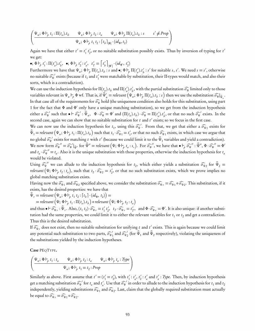
Ψu ; Φ p t1 :Π(ta).tb Ψu ; Φ p t2 : ta Ψu ; Φ p Π(ta).tb : s s ′ 6= Prop

Ψu ; Φ p t1 t2 : dtb e|Φ| · (idΦ, t2)

Again we have that either t ′ = t ′1 t ′2, or no suitable substitution possibly exists. Thus by inversion of typing for t ′

we get:•; Φ p t ′1 :Π(t ′a).t

′b , •; Φ p t ′2 : t ′a , t ′T =

t ′b£

|Φ′|· (idΦ′ , t ′2)

Furthermore we have that Ψu ; Φ p Π(ta).tb : s and •; Φ p Π(t′a).t

′b : s ′ for suitable s , s ′. We need s = s ′, otherwise

no suitable cσΨ′ exists (because if t1 and t ′1 were matchable by substitution, theirΠ-types would match, and also their

sorts, which is a contradiction).We can use the induction hypothesis forΠ(ta).tb andΠ(t ′a).t

′b , with the partial substitution cσΨ limited only to those

variables relevant inΨu p Φwf. That is, if bΨ′u = relevant�

Ψu ; Φ p Π(ta).tb : s�

then we use the substitution cσΨ|bΨu.

In that case all of the requirements for cσΨ hold (the uniqueness condition also holds for this substitution, using part1 for the fact that Φ and Φ′ only have a unique matching substitution), so we get from the induction hypothesiseither a cσΨ

′ such that • ` cσΨ′ : bΨu , Φ ·cσΨ = Φ′ and (Π(ta).tb ) ·cσΨ = Π(t ′a).t

′b , or that no such cσΨ

′ exists. In thesecond case, again we can show that no suitable substitution for t and t ′ exists; so we focus in the first case.We can now use the induction hypothesis for t1, using this cσΨ

′. From that, we get that either a cσΨ1 exists forbΨ1 = relevant

�

Ψu ; Φ p t1 :Π(ta).tb

�

such that t1 ·cσΨ1 = t ′1, or that no such cσΨ1 exists, in which case we argue that

no global cσΨ′ exists for matching t with t ′ (because we could limit it to the bΨ1 variables and yield a contradiction).

We now form cσΨ′′ = cσΨ

′|bΨ′′ for bΨ′′ = relevant

�

Ψ; Φ p ta : s∗�

. For cσΨ′′, we have that • p cσΨ

′′ : bΨ′′, Φ ·cσΨ′′ = Φ′

and ta ·cσΨ′′ = ta . Also it is the unique substitution with those properties, otherwise the induction hypothesis for ta

would be violated.Using cσΨ

′′ we can allude to the induction hypothesis for t2, which either yields a substitution cσΨ2 for bΨ2 =relevant

�

Ψ; Φ p t2 : ta

�

, such that t2 ·cσΨ2 = t ′2, or that no such substitution exists, which we prove implies noglobal matching substitution exists.Having now the cσΨ1 and cσΨ2 specified above, we consider the substitution cσΨ r =cσΨ1 ◦cσΨ2. This substitution, if itexists, has the desired properties: we have thatbΨr = relevant

�

Ψu ; Φ p t1 t2 : dtb e · (idΦ, t2)�

== relevant

�

Ψ; Φ p t1 :Π(ta).tb

�

◦ relevant�

Ψ; Φ p t2 : ta

�

and thus • `cσΨ r : bΨr . Also, (t1 t2) ·cσΨ r = t ′1 t ′2, tT ·cσΨ r = t ′T , and Φ ·cσΨ r =Φ′. It is also unique: if another substi-

tution had the same properties, we could limit it to either the relevant variables for t1 or t2 and get a contradiction.Thus this is the desired substitution.If cσΨ r does not exist, then no suitable substitution for unifying t and t ′ exists. This is again because we could limitany potential such substitution to two parts, cσΨ

′1 and cσΨ

′2 (for bΨ1 and bΨ2 respectively), violating the uniqueness of

the substitutions yielded by the induction hypotheses.

Case PEQTYPE.

Ψu ; Φ p t1 : ta Ψu ; Φ p t2 : ta Ψu ; Φ p ta : Type

Ψu ; Φ p t1 = t2 : Prop

Similarly as above. First assume that t ′ = (t ′1 = t ′2), with t ′1 : t ′a , t ′2 : t ′a and t ′a : Type. Then, by induction hypothesisget a matching substitution cσΨ

′ for ta and t ′a . Use that cσΨ′ in order to allude to the induction hypothesis for t1 and t2

independently, yielding substitutions cσΨ1 and cσΨ2. Last, claim that the globally required substitution must actuallybe equal to cσΨ r =cσΨ1 ◦cσΨ2.

93

Case PMETAVARUNIF.

Ψu .i = T T = [Φ∗] tT (i ≥ |Ψ|= 0) Ψu ; Φ p σ : Φ∗ Φ∗ ⊆ Φ σ = idΦ∗Ψu ; Φ p Xi/σ : tT ·σ

We trivially have tT ·σ = tT . We split cases depending on whether cσΨ.i is unspecified or not.

If bσ¯.i=?, then we split cases further depending on whether t ′ uses any variables higher than |Φ∗ ·cσΨ| − 1 or not.That is, if t ′ < f |Φ∗ · cσΨ| or not. In the case where this does not hold, it is obvious that there is no possiblecσΨ′ such that (Xi/σ) ·cσΨ

′ = t ′, since cσΨ′ must include cσΨ, and the term (Xi/σ) ·cσΨ

′ can therefore not includevariables outside the prefix Φ∗ · cσΨ of Φ · cσΨ. In the case where t ′ < f |Φ∗ · cσΨ|, we consider the substitutioncσΨ′ = cσΨ[i 7→ [Φ∗ · cσΨ] t ′]. In that case we obviously have Φ · cσΨ

′ = Φ′, tT · cσΨ′ = tT , and also t · cσΨ = t ′.

Also, bΨ′ = relevant�

Ψu ; Φ p Xi/σ : tT ·σ�

= (relevant�

Ψu ; Φ∗ p tT : s�

) ◦ relevant�

Ψ; Φ p σ : Φ∗�

◦ (Ψb@i).

We need to show that • `cσΨ′ : bΨ′. First, we have that relevant

�

Ψ; Φ p σ : Φ∗�

= relevant�

Ψ p Φwf�

since Φ∗ ⊆ Φ.

Second, we have that relevant�

Ψ; Φ p tT : s�

=

(relevant�

Ψu ; Φ∗ p tT : s�

) ◦ relevant�

Ψ p Φwf�

. Thus we have that bΨ′ = bΨ ◦ (Ψb@i). It is now trivial to see that

indeed • `cσΨ′ : bΨ′.

If bσ¯.i= t∗, then we split cases on whether t∗ = t ′ or not. If it is, then obviously cσΨ is the desired unifying substitu-tion for which all the desired properties hold. If it is not, then no substitution with the desired properties possiblyexists, because it would violate the uniqueness assumption for cσΨ.

Part 3 By inversion on the typing for T .

Case PEXTCTXTERM.

Ψu ; Φ p t : tT Ψu ; Φ ` tT : s

Ψu p [Φ] t : [Φ] tT

By inversion of typing for T ′ we have: T ′ = [Φ] t ′, •; Φ p t ′ : tT , •; Φ p tT : s .We thus have bΨu = relevant

�


= unspecΨu(since Φ is also well-formed in the empty extension con-

text), and the substitution cσΨ = unspecΨ is the unique substitution such that • `cσΨ : bΨu , Φ·cσΨ =Φ and tT ·cσΨ = tT .We can thus use part 2 for attempting a match between t and t ′, yielding a cσΨ

′ such that • ` cσΨ′ : bΨ′u with

bΨ′u = relevant�

Ψu ; Φ p t : tT

�

and t ·cσΨ′ = t ′. We have that relevant

�

Ψu ; Φ p t : tT

�

= relevant�

Ψu p T : K�

,

thus bΨ′u = Ψ by assumption. From that we realize that cσΨ′ is a fully-specified substitution since • ` cσΨ

′ : Ψ, andthus this is the substitution with the desired properties.If unification between t and t ′ fails, it is trivial to see that no substitution with the desired substitution exists,otherwise it would lead directly to a contradiction.

Case PEXTCTXINST.

Ψu p Φ, Φ′ wf

Ψu p [Φ]Φ′ : [Φ] ctx

By inversion of typing for T ′ we have: T ′ = [Φ]Φ′′, • p Φ, Φ′′ wf, • p Φ wf. From part 1 we get a cσΨ thatmatches Φ, Φ′ with Φ, Φ′′, or the fact that no such cσΨ exists. In the first case, as above, it is easy to see that this isthe fully-specified substitution that we desire. In the second case, no suitable substitution exists.

94

�The above proof is constructive. Its computational content is a pattern matching algorithm for patterns and

closed terms – the algorithm we presented earlier. Notice that the rules presented in Figures 5.10 through 5.12 followthe inductive structure of the proof and make the same assumption about types-of-types being subderivations. Basedon the statement of the above theorem, it is evident that this algorithm is sound (that is, if it finds a substitution,that substitution will be a matching substitution), and that it is also complete: if a matching substitution exists, thenthe algorithm will find it. The formal statement of soundness and completeness is as follows.

Lemma 5.1.11 (Pattern matching algorithm soundness and completeness)

1.

Ψu p Φwf • ` Φ′ wf relevant�

Ψu p Φwf�

= bΨu�

Ψu p Φwf�

∼�

• ` Φ′ wf�

.cσΨ

• `cσΨ : bΨu Φ ·cσΨ =Φ′

2.

Ψu p Φwf • ` Φ′ wf relevant�

Ψu p Φwf�

= bΨu

∃cσΨ.( • `cσΨ : bΨu Φ ·cσΨ =Φ′ )

�

Ψu p Φwf�

∼�

• ` Φ′ wf�

.cσΨ

3.


Ψu ; Φ p t : t ′T�

= bΨ′u�

Ψu ; Φ p tT : s •; Φ ` t ′T : s relevant�


= bΨu

�

∨�

tT = Type Ψu p Φwf • ` Φwf relevant�

Ψu p Φwf�

= bΨu

�

• `cσΨ : bΨu Φ ·cσΨ =Φ′ tT ·cσΨ = t ′T

�

Ψu ; Φ p t : tT

�

∼�

•; Φ′ ` t ′ : t ′T�

/cσΨ .cσΨ′

• `cσΨ′ : bΨ′u Φ ·cσΨ

′ =Φ′ tT ·cσΨ′ = t ′T t ·cσΨ

′ = t ′

4.


Ψu ; Φ p t : t ′T�

= bΨ′u�

Ψu ; Φ p tT : s •; Φ ` t ′T : s relevant�


= bΨu

�

∨�

tT = Type Ψu p Φwf • ` Φwf relevant�

Ψu p Φwf�

= bΨu

�

• `cσΨ : bΨu Φ ·cσΨ =Φ′ tT ·cσΨ = t ′T

∃cσΨ′.( • `cσΨ

′ : bΨ′u Φ ·cσΨ′ =Φ′ tT ·cσΨ

′ = t ′T t ·cσΨ′ = t ′ )

�

Ψu ; Φ p t : tT

�

∼�

•; Φ′ ` t ′ : t ′T�

/cσΨ .cσΨ′

5.

Ψu p T : K • ` T ′ : K relevant�

Ψu p T : K�

=Ψu�

Ψu p T : K�

∼�

• ` T ′ : K�

.cσΨ

• ` σΨ :Ψu T ·σΨ = T ′

6.

Ψu p T : K • ` T ′ : K relevant�

Ψu p T : K�

=Ψu

∃cσΨ.( • ` σΨ :Ψu T ·σΨ = T ′ )�

Ψu p T : K�

∼�

• ` T ′ : K�

.cσΨ

Proof. Valid by construction. �

95

(Annotated terms) t A ::= c | s | vL | bi | λ(t A1 ).t

A2 | Πs (t

A1 ).t

A2 | (t

A1 : t A : s) t A

2| t A

1 =t A t A2 | Xi/σ

(Annotated contexts) ΦA ::= • | ΦA, (t A : s) | ΦA, φi(Annotated extension terms) T A ::= [−] t A | [−]ΦA

Figure 5.13: Annotated λHOL terms (syntax)

Practical pattern matching. We can significantly simplify the presentation of the algorithm if instead of workingdirectly on typing derivations we work on annotated terms which we will define shortly. We will not do this onlyfor presentation purposes but for efficiency considerations too: the algorithm described so far would require us tokeep full typing derivations at runtime. Instead, we will extract the information required by the algorithm from thetyping derivations and make them available syntactically at the level of terms. The result will be the new notion ofannotated terms and an alternative formulation of the algorithm that works directly on such terms.

We present the syntax of annotated terms and annotated contexts in Figure 5.13. The main changes are:

1. the inclusion of sort information in Π-types,

2. type and sort information for functions in function application and

3. type information for the equality type.

Furthermore, each member of the context is annotated with its sort. Last, annotated extension terms do not needthe context information anymore – that information is only relevant for typing purposes. We adapt the patternmatching rules so that they work on annotated terms instead in Figure 5.14. The algorithm accepts Ψu as animplicit argument in order to know what the length of the resulting substitution needs to be.

A well-typed annotated term t A is straightforward to produce from a typing derivation of a normal term t ; theinverse is also true. In the rest, we will thus use the two kinds of terms interchangeably and drop the A superscriptwhen it is clear from context which kind we mean. For example, we will use the algorithm of Figure 5.14 algorithmdirectly to decide pattern matching between a well-typed pattern t and a scrutinee t ′. It is understood that thesehave been converted to annotated terms after typing as needed. We give the exact rules for the conversion in Figure5.15 as a type derivation-directed translation function.

We prove the following lemma about the correspondence between the two algorithms working on derivationsand annotated terms; then soundness and completeness for the new algorithm follows directly.

Lemma 5.1.12 (Correspondence between pattern matching algorithms)

1.

�

Ψu p T : K�

∼�

• ` T ′ : K�

.cσΨ ¹Ψu ` T : KºA= T A �

• ` T ′ : K�A= T ′A

T A∼ T ′A .¹• `cσΨ :ΨuºA

2.¹Ψu ` T : KºA= T A �

• ` T ′ : K�A= T ′A T A∼ T ′A .cσΨ

A

∃cσΨ.( ¹• `cσΨ :ΨuºA=cσΨ

A�

Ψu p T : K�

∼�

• ` T ′ : K�

.cσΨ )

96

T ∼ T ′ .cσΨ

t ∼ t ′ / unspecΨu.cσΨ

[−] t ∼ [−] t ′ .cσΨ

Φ′ ∼ Φ′′ .cσΨ[−]Φ′ ∼ [−]Φ′′ .cσΨ

Φ′ ∼ Φ′′ .cσΨ

• ∼ • . unspecΨu

s = s ′ Φ∼ Φ′ .cσΨ t ∼ t ′ /cσΨ .cσΨ′

(Φ, (t : s))∼ (Φ′, (t ′ : s ′)) .cσΨ′ �

Φ, φi�

∼�

Φ,Φ′�

. unspecΨu[i 7→ [−]Φ′]

t ∼ t ′ /cσΨ .cσΨ′

c ∼ c /cσΨ .cσΨ s ∼ s /cσΨ .cσΨ

L ·cσΨ = L′

vL ∼ v ′L /cσΨ .cσΨ

s = s ′ t1 ∼ t ′1 /cσΨ .cσΨ′ dt2e ∼

t ′2£

/cσΨ′ .cσΨ

′′

Πs (t1).t2 ∼Πs ′(t′1).t

′2 /cσΨ .cσΨ

′′

dt2e ∼

t ′2£

/cσΨ .cσΨ′

λ(t1).t2 ∼ λ(t′1).t

′2 /cσΨ .cσΨ

′

s = s ′ t ∼ t ′ /cσΨ .cσΨ′

t1 ∼ t ′1 /cσΨ′ .cσΨ1 t2 ∼ t ′2 /cσΨ

′ .cσΨ2 cσΨ1 ◦cσΨ2 =cσΨ′′

((t1 : t : s) t2)∼�

(t ′1 : t ′ : s ′) t ′2�

/cσΨ .cσΨ′′

t ∼ t ′ /cσΨ .cσΨ′ t1 ∼ t ′1 /cσΨ

′ .cσΨ1 t2 ∼ t ′2 /cσΨ′ .cσΨ2 cσΨ1 ◦cσΨ2 =cσΨ

′′

�

t1 =t t2�

∼�

t ′1 =t ′ t ′2�

/cσΨ .cσΨ′′

cσΨ.i =? t ′ < f |σ ·cσΨ|Xi/σ ∼ t ′ /cσΨ .cσΨ[i 7→ [−] t ′]

cσΨ.i = t ′

Xi/σ ∼ t ′ /cσΨ .cσΨ

Figure 5.14: Pattern matching algorithm for λHOL, operating on annotated terms

97

¹• ` T : KºA= T A

¹Ψ; Φ ` t : tTºA= t A

¹Ψ ` [Φ] t : [Φ] tTºA= [−] t A

�

Ψ ` Φ, Φ′ wf�A=ΦA, Φ′A

�

Ψ ` [Φ]Φ′ : [Φ] ctx�A= [−]Φ′A

�

• ` Φwf�A=ΦA

�

Ψ ` •wf�A= •

�

Ψ ` Φwf�A=ΦA

¹Ψ; Φ ` t : sºA= t A

�

Ψ ` (Φ, t )wf�A= (ΦA, (t A : s))

�

Ψ ` Φwf�A=ΦA

�

Ψ ` Φ, φi wf�A= (ΦA, φi )

�

Ψ; Φ ` t : t ′�A= t A

¹Ψ; Φ ` c : tºA= c�

Ψ; Φ p s : s ′�A= s

�

Ψ; Φ p vL : t�A= vL

�

Ψ; Φ p t1 : s�A= t A

1

�

Ψ; Φ, t1 p dt2e|Φ| : s ′�A=

t A2

£

�

Ψ; Φ `Π(t1).t2 : s ′′�A=Πs (t

A1 ).t

A2

¹Ψ; Φ ` t1 : sºA= t A1

�

Ψ; Φ, t1 ` dt2e|Φ| : t ′�A= dt2e

A

�

Ψ; Φ ` λ(t1).t2 :Π(t1).�

t ′�

|Φ|õ1

�A= λ(t A

1 ).tA2

¹Ψ; Φ ` t1 :Π(ta).tbºA= t A

1 ¹Ψ; Φ ` t2 : taºA= t A

2 ¹Ψ; Φ `Π(ta).tb : sºA= t A

�

Ψ; Φ ` t1 t2 : dtb e|Φ| · (idΦ, t2)�A= (t A

1 : t A : s) t A2

�

Ψu ; Φ p t : Type�A= t A

�

Ψu ; Φ p t1 : t�A= t A

1

�

Ψu ; Φ p t2 : t�A= t A

2�

Ψu ; Φ p t1 = t2 : Prop�A= (t A

1 =t A t A2 )

�

Ψu ; Φ p Xi/σ : tT ·σ�A=Xi/σ

Figure 5.15: Conversion of typing derivations to annotated terms

98

3.

�

Ψu p Φwf�

∼�

• ` Φ′ wf�

.cσΨ ¹Ψu ` ΦwfºA=ΦA �

• ` Φ′ wf�A=Φ′A

ΦA∼ Φ′A .¹• `cσΨ :ΨuºA

4.¹Ψu ` ΦwfºA=ΦA �

• ` Φ′ wf�A=Φ′A ΦA∼ Φ′A=cσΨ

A

∃cσΨ.( ¹• `cσΨ :ΨuºA .cσΨ

A�

Ψu p Φwf�

∼�

• ` Φ′ wf�

.cσΨ )

5.

�

Ψu ; Φ ` t : tT�

∼�

•; Φ′ ` t ′ : t ′T�

/cσΨ .cσΨ′

¹Ψu ; Φ ` t : tTºA= t A

�

•; Φ′ ` t ′ : t ′T�A= t ′A

�

• `cσΨ : bΨ�A=cσΨ

A

t A∼ t ′A /cσΨA .�

• `cσΨ′ : bΨ′

�A

6.¹Ψu ; Φ ` t : tTº

A= t A�

•; Φ′ ` t ′ : t ′T�A= t ′A

�

• `cσΨ : bΨ�A=cσΨ

A t A∼ t ′A /cσΨA .cσΨ

′A

∃cσΨ.(�

• `cσΨ′ : bΨ′

�A.cσΨ

′A �

Ψu ; Φ ` t : tT�

∼�

•; Φ′ ` t ′ : t ′T�

/cσΨ .cσΨ′ )

Proof. By structural induction on the derivation of the pattern matching result. We also need to use Lemma 5.1.1.�

Lemma 5.1.13 (Soundness and completeness for practical pattern matching algorithm)

1.

Ψu p T : K ¹Ψu ` T : KºA= T A

• ` T ′ : K�

• ` T ′ : K�A= T ′A relevant

�

Ψu p T : K�

=Ψu T ∼ T ′ . σAΨ

∃σΨ.( • ` σΨ :Ψu ¹• ` σΨ :ΨuºA= σA

Ψ T ·σΨ = T ′ )

2.

Ψu p T : K¹Ψu ` T : KºA= T A • ` T ′ : K

�

• ` T ′ : K�A= T ′A relevant

�

Ψu p T : K�

=Ψu

∃σΨ.( • ` σΨ :Ψu T ·σΨ = T ′ )

T ∼ T ′ .¹• ` σΨ :ΨuºA

Proof. By combining Lemma 5.1.11, Lemma 5.1.12 and Lemma 5.1.1. �

Summary

Let us briefly summarize the results of this section. For the typing judgement we defined in the end of Section 5.1,as follows:

Ψ p Ψu wf Ψ, Ψu p TP : K unspecΨ,Ψu v relevant�

Ψ, Ψu p TP : K�


we have the following results:


Ψ′ ∗p Ψu ·σΨ > TP ·σΨ : K ·σΨSUBSTITUTION LEMMA

• ∗p Ψu > TP : K • ` T : K

∃≤1σΨ.( • ` σΨ :Ψu TP ·σΨ = T )

PATTERN MATCHING

DETERMINISM AND DECIDABILITY

99

• ∗p Ψu > TP : K • ` T : K TP ∼ T = σΨ

• ` σΨ :Ψu TP ·σΨ = T

PATTERN MATCHING

ALGORITHM SOUNDNESS

• ∗p Ψu > TP : K • ` T : K

∃σΨ.( • ` σΨ :Ψu TP ·σΨ = T )

TP ∼ T = σΨ

PATTERN MATCHING

ALGORITHM COMPLETENESS

5.2 Collapsing extension variables

Let us consider the following situation. We are writing a tactic such as the simplify tactic given in Section 2.3 underthe heading “Staging”, a sketch of which is (using the new notations for extension types):

simplify : (φ : ctx)→ (P : [φ]Prop)→ (Q : [φ]Prop, [φ]P ⊃Q ∧Q ⊃ P )

simplify P = match P withQ ∧R⊃O 7→ ⟨Q ⊃ R⊃O, · · · ⟩

In order to fill the missing proof object (denoted as · · · ), we need to perform pattern matching on its inferred type:the open proposition

[φ] ((Q ∧R⊃O)⊃ (Q ⊃ R⊃O))∧ ((Q ⊃ R⊃O)⊃ (Q ∧R⊃O))

in the extension context Ψ that includes φ, P, Q, R, O. Yet the pattern matching procedure presented in theprevious section is only applicable when the extension context is empty. Instead of changing our pattern matchingprocedure, we notice that we can prove an equivalent first-order lemma instead where only normal logical variablesare used (and is therefore closed with respect to Ψ):

[P : Prop,Q : Prop, R : Prop,O : Prop] ((Q ∧R⊃O)⊃ (Q ⊃ R⊃O))∧ ((Q ⊃ R⊃O)⊃ (Q ∧R⊃O))

Then, by instantiating this lemma with the variables of the open Ψ at hand, we can get a proof of the desired type.But is there always such an equivalent first-order lemma in the general case of extension contexts Ψ and can we findit if one exists? This will be the subject of this section.

More formally, we want to produce a proof object for a proposition P at a point where the extension variablescontext is Ψ. If we want to discover this proof object programmatically, we need to proceed by pattern matchingon P (as the scrutinee). A problem arises: P is not closed, so the pattern matching methodology presented in theprevious section does not apply – since only patterns are allowed to use extension variables (as unification variables).That is, we need to solve the following problem:

If Ψ, Ψu p PP : [Φ]Prop and Ψ ` P : [Φ]Prop,then there exists σΨ such that Ψ ` σΨ : (Ψ, Ψu ) and PP ·σΨ = P.

This is a significantly more complicated pattern matching problem, because P also contains meta-variables. Tosolve it properly, we need to be able to have unification variables that match against meta-variables; these unificationvariables will then be meta-2-variables.

In this section we will partially address this issue in a different way. We will show that under certain restrictionsabout the current non-empty extension contextΨ and its usage, we can collapse terms fromΨ to an empty extensioncontext. A substitution exists that then transforms the collapsed terms into terms of the original Ψ context. That

100

collapsable (Ψ) /Φ .Φ′

collapsable (•) /Φ .Φcollapsable (Ψ) /Φ .Φ′ collapsable (K) /Φ′ .Φ′′

collapsable (Ψ, K) /Φ .Φ′′

collapsable (K) /Φ′ .Φ′′

T = [Φ] t collapsable (T ) /Φ′ .Φ′′

collapsable ([Φ] t ) /Φ′ .Φ′′collapsable (Φ) /Φ′ .Φ′′

collapsable ([Φ] ctx) /Φ′ .Φ′′

collapsable (T ) /Φ′ .Φ′′

collapsable (Φ) /Φ′ .Φ′′ collapsable (t ) /Φ′′

collapsable ([Φ] t ) /Φ′ .Φ′′collapsable (Φ1, Φ2) /Φ

′ .Φ′′

collapsable ([Φ1]Φ2) /Φ′ .Φ′′

collapsable (Ψ ` T : K) .Φ′

collapsable (Ψ) / • .Φ′ collapsable (K) /Φ′ .Φ′′ collapsable (T ) /Φ′′ .Φ′′

collapsable (Ψ ` T : K) .Φ′′

collapsable�

Ψ ` Φwf�

.Φ′

collapsable (Ψ) / • .Φ′ collapsable (Φ) /Φ′ .Φ′′

collapsable�

Ψ ` Φwf�

.Φ′′

Figure 5.16: Operation to decide whether λHOL terms are collapsable with respect to the extension context

is, we can get an equivalent term that is closed with respect to the extension context and use our normal patternmatching procedure on that.

We will thus prove the following theorem for contextual terms:

Ψ; Φ ` t : t ′ collapsable�

Ψ ` [Φ] t : [Φ] t ′�

∃t↓, t ′↓,Φ↓,σ .( •; Φ↓ ` t↓ : t ′↓ Ψ; Φ ` σ : Φ↓ t↓ ·σ = t t ′↓ ·σ = t ′ )

Combined with the pattern matching algorithm given in the previous section, which applies when Ψ= •, this willgive us a way to perform pattern matching even when Ψ is not empty under the restrictions that we will express asthe “collapsable” operation.

Let us now see the details of the limitations in the applicability of our solution. Intuitively, we will be able tocollapse the extension variable context when all extension variables depend on contextsΦwhich are prefixes of someΦ′ context. The collapsable operation is actually a function that discovers such a context, if it exists. Furthermore,all uses of extension variables should be used only with identity substitutions. This restriction exists because thereis no generic way of encoding the equalities that are produced by non-identity substitutions. We present the fulldetails of the collapsable function in Figures 5.16 and 5.17.

The actual collapsing transformation amounts to replacing all instances of meta-variables with normal variables,instantiating all context variables with the empty context, and renaming normal variables appropriately, so thatboth meta-variables and normal variables can refer to one identical Φ context. We can define this transformation

101

collapsable (Φ) /Φ′ .Φ′′

collapsable (•) /Φ′ .Φ′collapsable (Φ) /Φ′ .Φ′′ Φ=Φ′′ collapsable (t ) /Φ

collapsable (Φ, t ) /Φ′ . (Φ, t )

collapsable (Φ) /Φ′ .Φ′′ Φ⊂ Φ′′ collapsable (t ) /Φ′′

collapsable (Φ, t ) /Φ′ .Φ′′collapsable (Φ) /Φ′ .Φ′′ Φ=Φ′′

collapsable�

Φ, φi�

/Φ′ . (Φ, φi )

collapsable (Φ) /Φ′ .Φ′′ Φ⊂ Φ′′

collapsable�

Φ, φi�

/Φ′ .Φ′′

collapsable (t ) /Φ′

collapsable (s) /Φ′ collapsable (c) /Φ′ collapsable (vL) /Φ′

collapsable (t1) /Φ′ collapsable (t2) /Φ

′

collapsable (λ(t1).t2) /Φ′


′

collapsable (Π(t1).t2) /Φ′


′

collapsable (t1 t2) /Φ′


′

collapsable (t1 = t2) /Φ′

σ ⊆ idΦcollapsable

�

Xi/σ�

/Φ′

Figure 5.17: Operation to decide whether λHOL terms are collapsable with respect to the extension context (con-tinued)

102

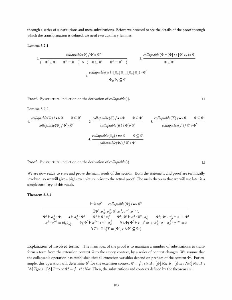
through a series of substitutions and meta-substitutions. Before we proceed to see the details of the proof throughwhich the transformation is defined, we need two auxiliary lemmas.

Lemma 5.2.1

1.collapsable (Φ) /Φ′ .Φ′′

( Φ′ ⊆ Φ Φ′′ =Φ ) ∨ ( Φ⊆ Φ′ Φ′′ =Φ′ )2.

collapsable (Ψ ` [Φ] t : [Φ] tT ) .Φ′

Φ⊆ Φ′

3.collapsable (Ψ ` [Φ0]Φ1 : [Φ0]Φ1) .Φ

′

Φ0,Φ1 ⊆ Φ′

Proof. By structural induction on the derivation of collapsable (·). �

Lemma 5.2.2

1.collapsable (Ψ) / • .Φ Φ⊆ Φ′

collapsable (Ψ) /Φ′ .Φ′2.

collapsable (K) / • .Φ Φ⊆ Φ′

collapsable (K) /Φ′ .Φ′3.

collapsable (T ) / • .Φ Φ⊆ Φ′

collapsable (T ) /Φ′ .Φ′

4.collapsable (Φ0) / • .Φ Φ⊆ Φ′

collapsable (Φ0) /Φ′ .Φ′

Proof. By structural induction on the derivation of collapsable (·). �

We are now ready to state and prove the main result of this section. Both the statement and proof are technicallyinvolved, so we will give a high-level picture prior to the actual proof. The main theorem that we will use later is asimple corollary of this result.

Theorem 5.2.3

`Ψwf collapsable (Ψ) / • .Φ0

∃Ψ1,σ1Ψ,σ2

Ψ,Φ1,σ1,σ−1,σ i nv .Ψ1 ` σ1

Ψ :Ψ • ` σ2Ψ :Ψ1 Ψ1 ` Φ1 wf Ψ1; Φ1 ` σ1 : Φ0 ·σ1

Ψ Ψ1; Φ0 ·σ1Ψ ` σ

−1 : Φ1

σ1 ·σ−1 = idΦ0·σ1Ψ

Ψ; Φ0 ` σ i nv : Φ1 ·σ2Ψ ∀t .Ψ; Φ0 ` t : t ′⇒ t ·σ1

Ψ ·σ1 ·σ2

Ψ ·σi nv = t

∀T ∈Ψ1.(T = [Φ∗] t ∧Φ∗ ⊆ Φ1)

Explanation of involved terms. The main idea of the proof is to maintain a number of substitutions to trans-form a term from the extension context Ψ to the empty context, by a series of context changes. We assume thatthe collapsable operation has established that all extension variables depend on prefixes of the context Φ0. For ex-ample, this operation will determine Φ0 for the extension context Ψ = φ : ctx,A : [φ]Nat,B : [φ, x : Nat]Nat,T :[φ]Type, t : [φ]T to be Φ0 =φ, x0 : Nat. Then, the substitutions and contexts defined by the theorem are:

103

Φ1 is a context that is composed of ‘collapsed’ versions of all extension variables, as well as any normal variablesrequired to type them. For the above example, this would be determined as Φ1 = A1 : Nat, x1 : Nat, B1 : Nat, T 1 :Type, t 1 : T 1.

Ψ1 is an extension context where all extension variables depend on the Φ1 context. It has the same metavariables asΨ, with the difference that all of them use prefixes of the Φ1 context and dependencies on previous meta-variablesare changed to dependencies on the Φ1 context. Context variables are also elided. For the above example contextwe will therefore have Ψ1 = A′ : [Φ1]Nat,B ′ : [Φ1]Nat,T ′ : [Φ1]Type, t ′ : [Φ1]T 1, where we use primed names formeta-variables to distinguish them from the normal ones of Ψ.

σ1Ψ can be understood as a renaming of metavariables from the original Ψ context to the Ψ1 context. Since the

two contexts have essentially the same metavariables, the renaming is simple to carry out. Context variables aresubstituted with the empty context. This is fine since parametric contexts carry no information. For the examplecontext above, we will have that σ1

Ψ =φ 7→ •,A 7→A′,B 7→ B ′,T 7→ T ′, t 7→ t ′

σ1 can be understood as a permutation from variables in Φ0 to variables in Φ1. The need for it arises from the factthat collapsed versions of metavariables get interspersed with normal variables in Φ1. σ−1 is the permutation for theinverse direction, that is from variables in Φ1 to variables in Φ0. For the example, we have:σ1 = x0 7→ x1

σ−1 =A1 7→A′, x1 7→ x0, B1 7→ B ′, T 1 7→ T ′, t 1 7→ t ′

σ2Ψ carries out the last step, which is to replace the extension variables from Ψ1 with their collapsed versions in theΦ1 context. In the example, we would have that σ2

Ψ =A′ 7→ [Φ1]A1, B ′ 7→ [Φ1]B1, T ′ 7→ [Φ1]T 1, t ′ 7→ [Φ1] t 1.σ i nv is the substitution that inverses all the others, yielding a term in the originalΨ extension context from a closedcollapsed term. In the example this would be σ i nv =A1 7→A, x1 7→ x0, B1 7→ B , T 1 7→ T , t 1 7→ t .

Proof. By induction on the derivation of the relation collapsable (Ψ) / • .Φ0.

Case Ψ = •. We choose Ψ1 = •; σ1Ψ = σ

2Ψ = •; Φ

1 = •; σ1 = σ−1 = •; σ i nv = • Φ1 = • and the desired triviallyhold.

Case Ψ=Ψ′, [Φ]ctx. From the collapsable relation, we get: collapsable�

Ψ′�

/•.Φ′0, collapsable ([Φ] ctx)/Φ′0 .Φ0.By induction hypothesis for Ψ′, get:Ψ′1 ` σ ′1Ψ :Ψ′ • ` σ ′2Ψ :Ψ′1 Ψ′1 ` Φ′1 wf Ψ′1; Φ′1 ` σ ′1 : Φ′0 ·σ ′1Ψ Ψ′1; Φ′0 ·σ ′1Ψ ` σ

′−1 : Φ′1

σ ′1 ·σ ′−1 = idΦ′0·σ ′1Ψ Ψ′; Φ′0 ` σ ′i nv : Φ′1 ·σ ′2Ψ ∀t .Ψ′; Φ′0 ` t : t ′⇒ t ·σ ′1Ψ ·σ′1 ·σ ′2Ψ ·σ

′i nv = t

∀T ∈Ψ′1.T = [Φ∗] t ∧Φ∗ ⊆ Φ′1

By inversion of typing for [Φ] ctx we get that Ψ′ ` Φwf.We fix σ1

Ψ = σ′1Ψ , [Φ′0 ·σ ′1Ψ ]• which is a valid choice as long as we select Ψ1 so that Ψ′1 ⊆ Ψ1. This substitution has

correct type by taking into account the substitution lemma for Φ′0 and σ ′1Ψ .For choosing the rest, we proceed by induction on the derivation of Φ′0 ⊆ Φ0.

If ˘0 = ˘′0 then:We have Φ⊆ Φ′0 because of Lemma 5.2.1.Choose Ψ1 =Ψ′1 ; σ2

Ψ = σ′2Ψ ; Φ1 =Φ′1 ; σ1 = σ ′1 ; σ−1 = σ ′−1; σ i nv = σ ′i nv .

Everything holds trivially, other than σ1Ψ typing. This too is easy to prove by taking into account the substitution

lemma for Φ and σ ′1Ψ . Also, σ ′i nv typing uses extension variable weakening. Last, for the cancellation part, termsthat are typed under Ψ are also typed under Ψ′ so this part is trivial too.

104

If ˘0 = ˘′0, t then: (here we abuse notation slightly by identifying the context and substitutions from inductionhypothesis with the ones we already have: their properties are the same for the new Φ′0)We have Φ=Φ0 =Φ′0, t because of Lemma 5.2.1 (Φ0 is not Φ′0 thus Φ0 =Φ).First, choose Φ1 =Φ′1, t ·σ ′1Ψ ·σ

′1. This is a valid choice, becauseΨ′; Φ′0 ` t : s ; by applying σ ′1Ψ we getΨ′1; Φ′0 ·σ ′1Ψ `t ·σ ′1Ψ : s ; by applying σ ′1 we get Ψ′1; Φ′1 ` t ·σ ′1Ψ ·σ

′1 : s .Thus Ψ′1 ` Φ′1, t ·σ ′1Ψ ·σ

′1 wf.Now, choose Ψ1 =Ψ′1, [Φ1] t ·σ ′1Ψ ·σ

′1. This is well-formed because of what we proved above about the substitutedt , taking weakening into account. Also, the condition for the contexts in Ψ1 being subcontexts of Φ1 obviouslyholds.Choose σ2

Ψ = σ′2Ψ , [Φ1]v|Φ′1|. We have • ` σ2

Ψ :Ψ1 directly by our construction.Choose σ1 = σ ′1, v|Φ′1|. We have that this latter term can be typed as:Ψ1; Φ1 ` v|Φ′1| : t ·σ ′1Ψ ·σ

′1, and thus we have Ψ1; Φ1 ` σ1 : Φ′0 ·σ ′1Ψ , t ·σ ′1Ψ .Choose σ−1 = σ ′−1, v|Φ′0·σ ′1Ψ |. The desired properties obviously hold.Choose σ i nv = σ ′i nv , v|Φ′0|, which is typed correctly since t ·σ ′1Ψ ·σ

′1 ·σ ′2Ψ ·σi nv = t .

Last, assume Ψ; Φ′0, t ` t∗ : t ′∗. We prove t∗ ·σ1Ψ ·σ

1 ·σ2Ψ ·σ

i nv = t∗.

First, t∗ is also typed under Ψ′ because t∗ cannot use the newly-introduced variable directly (even in the casewhere it would be part of Φ0, there’s still no extension variable that has X|Ψ′| in its context).Thus it suffices to prove t∗ ·σ ′1Ψ ·σ

1 ·σ2Ψ ·σ

i nv = t∗.Then proceed by structural induction on t∗. The only interesting case occurs when t∗ = v|Φ′0|, in which casewe have:v|Φ′0| ·σ ′1Ψ ·σ

1 ·σ2Ψ ·σ

i nv = v|Φ′0·σ ′1Ψ | ·σ1 ·σ2

Ψ ·σi nv = v|Φ′1| ·σ2

Ψ ·σi nv = v|Φ′1·σ2

Ψ|·σ i nv = v|Φ′0|

If ˘0 = ˘′0, φi then:By well-formedness inversion we get that Ψ.i = [Φ∗] ctx, and by repeated inversions of the collapsable relation weget Φ∗ ⊆ Φ′0.Choose Φ1 =Φ′1 ; Ψ1 =Ψ′1 ; σ2

Ψ = σ′2Ψ ; σ1 = σ ′1; σ−1 = σ ′−1; σ i nv = σ ′i nv .

Most desiderata are trivial. For σ1, note that (Φ′1, φi ) ·σ ′1Ψ =Φ′1 ·σ ′1Ψ since by construction we have that σ ′1Ψ always

substitutes parametric contexts by the empty context.For substitutions cancellation, we need to prove that for all t such that Ψ; Φ′0, φi ` t∗ : t ′∗, we have t∗ · σ1

Ψ · σ1 ·

σ2Ψ ·σ

i nv = t∗. This is proved directly by noticing that t∗ is typed also under Ψ′ (φi as the just-introduced variablecannot refer to itself).

Case Ψ=Ψ′, [Φ] t . From the collapsable relation, we get:collapsable

�

Ψ′�

/ • .Φ′0, collapsable (Φ) /Φ′0 .Φ0, collapsable (t ) /Φ0.By induction hypothesis for Ψ′, we get:Ψ′1 ` σ ′1Ψ :Ψ′ • ` σ ′2Ψ :Ψ′1 Ψ′1 ` Φ′1 wf Ψ′1; Φ′1 ` σ ′1 : Φ′0 ·σ ′1Ψ Ψ′1; Φ′0 ·σ ′1Ψ ` σ

′−1 : Φ′1

σ ′1 ·σ ′−1 = idΦ′0·σ ′1Ψ Ψ′; Φ′0 ` σ ′i nv : Φ′1 ·σ ′2Ψ ∀t .Ψ′; Φ′0 ` t : t ′⇒ t ·σ ′1Ψ ·σ′1 ·σ ′2Ψ ·σ

′i nv = t

∀T ∈Ψ′1.T = [Φ∗] t ∧Φ∗ ⊆ Φ′1

Also from typing inversion we get: Ψ′ ` Φwf and Ψ′; Φ ` t : s .We proceed similarly as in the previous case, by induction onΦ′0 ⊆ Φ0, in order to redefineΨ′1,σ ′1Ψ ,σ ′2Ψ ,Φ′1,σ ′1,σ ′−1,σ i nv

with the same properties but for Φ0 instead of Φ′0:Ψ′1 ` σ ′1Ψ :Ψ′ • ` σ ′2Ψ :Ψ′1 Ψ′1 ` Φ′1 wf Ψ′1; Φ′1 ` σ ′1 : Φ0 ·σ ′1Ψ Ψ′1; Φ0 ·σ ′1Ψ ` σ

′−1 : Φ′1

σ ′1 ·σ ′−1 = idΦ0·σ ′1ΨΨ′; Φ0 ` σ ′i nv : Φ′1 ·σ ′2Ψ ∀t .Ψ′; Φ0 ` t : t ′⇒ t ·σ ′1Ψ ·σ

′1 ·σ ′2Ψ ·σ′i nv = t

∀T ∈Ψ′1.T = [Φ∗] t ∧Φ∗ ⊆ Φ′1

105

Now we have Φ⊆ Φ0 thus Ψ′; Φ0 ` t : s .By applying σ ′1Ψ and then σ ′1 to t we get Ψ′1; Φ′1 ` t ·σ ′1Ψ ·σ

′1 : s . We can now choose Φ1 =Φ′1, t ·σ ′1Ψ ·σ′1.

Choose Ψ1 =Ψ′1, [Φ1] t ·σ ′1Ψ ·σ′1. It is obviously well-formed.

Choose σ1Ψ = σ

′1Ψ , [Φ] t 1. We need Ψ1; Φ ·σ ′1Ψ ` t 1 : t ·σ ′1Ψ .

Assuming t 1 =X|Φ′1|/σ , we need t ·σ ′1Ψ ·σ′1 ·σ = t ·σ ′1Ψ and Ψ1; Φ ·σ ′1Ψ ` σ : Φ1.

Therefore σ = σ ′−1 and σ1Ψ = σ

′1Ψ , [Φ]X|Φ′1|/σ

′−1 with the desirable properties.Choose σ2

Ψ = σ′2Ψ , [Φ1]v|Φ′1|. We trivially have • ` σ2

Ψ :Ψ1.Choose σ1 = σ ′1, with typing holding obviously.Choose σ−1 = σ−1, X|Ψ′1|/idΦ1 . Since σ1 does not use the newly introduced variable in Φ1, the fact that σ−1 is itsinverse follows trivially.Choose σ i nv = σ ′i nv , X|Ψ′|/id(Φ). This is well-typed if we consider the substitutions cancellation fact.It remains to prove that for all t∗ such that Ψ′,[Φ] t ; Φ0 ` t∗ : t ′∗, we have t∗ ·σ1

Ψ ·σ1 ·σ2

Ψ ·σi nv = t∗.

This is done by structural induction on t∗, with the interesting case being t∗ =X|Ψ′|/σ∗. By inversion of collapsablerelation, we get that σ∗ = idΦ.Thus (X|Ψ′|/idΦ) ·σ1

Ψ ·σ1 ·σ2

Ψ ·σi nv = (X|Φ′1|/(idΦ ·σ1

Ψ)) ·σ1 ·σ2

Ψ ·σi nv = (X|Φ′1|/(idΦ·σ1

Ψ)) ·σ1 ·σ2

Ψ ·σi nv = (X|Φ′1|/(idΦ·σ1

Ψ·

σ1)) ·σ2Ψ ·σ

i nv = (X|Φ′1|/(idΦ1)) ·σ2Ψ ·σ

i nv = (v|Φ′1| ·(idΦ1 ·σ2Ψ)) ·σ

i nv = (v|Φ′1| ·idΦ1·σ2Ψ) ·σ i nv = v|Φ′1·σ2

Ψ|·σ i nv =X|Ψ′|/idΦ.

�

Theorem 5.2.4

Ψ ` [Φ] t : [Φ] tT collapsable (Ψ ` [Φ] t : [Φ] tT ) .Φ∗

∃Φ′, t ′, t ′T ,σ .• ` Φ′ wf • ` [Φ′] t ′ : [Φ′] t ′T Ψ; Φ ` σ : Φ′ t ′ ·σ = t t ′T ·σ = tT

Proof. Trivial application of Theorem 5.2.3. Set Φ′ =Φ1 ·σ2Ψ, t ′ = t ·σ1

Ψ ·σ1 ·σ2

Ψ, t ′T = tT ·σ1Ψ ·σ

1 ·σ2Ψ, and also

set σ = σ−1. �

106

Chapter 6

The VeriML computational language

Having presented the details of the λHOL logic and its associated operations in the previous chapters, we are nowready to define the core VeriML computational language. I will first present the basic constructs of the language forintroducing and manipulating λHOL logical terms. I will state the type safety theorem for this language and proveit using the standard syntactic approach of Wright and Felleisen [1994]. I will then present some extensions to thelanguage that will be useful for the applications of VeriML we will consider in the rest.

6.1 Base computation language

6.1.1 Presentation and formal definition

The core of VeriML is a functional language with call-by-value semantics and support for side-effects such as mutablereferences in the style of ML. This core calculus is extended with constructs that are tailored to working with termsof the λHOL logic. Specifically, we include constructs in order to be able to introduce extension terms T – thatis, contextual terms and contexts – and also to look into their structure through pattern matching. The type K ofan extension term T is retained at the level of VeriML computational types. Types K can mention variables fromthe extension context Ψ and can therefore depend on terms that were introduced earlier. Thus λHOL constructsavailable at the VeriML level are dependently typed. We will see more details of this in the rest of this section.

Let us now present the formal details of VeriML, split into the ML core and the λHOL-related extensions.Figure 6.1 defines the syntax of the ML core of VeriML; Figures 6.3 through 6.5 give the relevant typing rulesand Figure 6.8 gives the small-step operational semantics. This ML core supports the following features: higher-order functional programming (through function types τ1→ τ2); general recursion (through the fixpoint constructfix x : τ.e); algebraic data types (combining product types τ1× τ2, sum types τ1+ τ2, recursive types µα : k .τ andthe unit type unit); mutable references ref τ; polymorphism over types supporting full System F – also referred toas rank-N-polymorphism (through the ∀α : k .τ type); and type constructors in the style of System Fω (by includingarrows at the kind level k1→ k2 and type constructors λα : k .τ at the type level). Data type definitions of the form:

data list α=Nil | Cons of α× list α

can be desugared to their equivalent using the base algebraic data type formers:

let list= λα : ?.µlist : ?.unit+α× listlet Nil= λα : ?.fold (inj1 ())let Cons= λα : ?.λhd : α.λtl : list α.fold (inj2 (hd, tl))

107

(Kinds) k ::= ? | k→ k(Types) τ ::= unit | τ1→ τ2 | τ1×τ2 | τ1+τ2 | µα : k .τ | ref τ

| ∀α : k .τ | λα : k .τ | τ1 τ2 | α(Expressions) e ::= () | λx : τ.e | e e ′ | x | (e , e ′) | proji e | inji e

| case(e , x.e ′, x.e ′′) | fold e | unfold e | ref e | e := e ′ | !e | l| Λα : k .e | e τ | fix x : τ.e

(Contexts) Γ ::= • | Γ, x : τ | Γ, α : k(Values) v ::= () | λx : τ.e | (v, v ′) | inji v | fold v | l | Λα : k .e

(Evaluation contexts) E ::= • | E e ′ | v E | (E , e) | (v, E) | proji E | inji E| case(E , x.e1, x.e2) | fold E | unfold E | ref E | E := e ′

| v := E | !E | E τ(Stores) µ ::= • | µ, l 7→ v

(Store typing) M ::= • |M, l : τ

Figure 6.1: VeriML computational language: ML core (syntax)

(Kinds) k ::= · · · | ΠV : K .k(Types) τ ::= · · · | (V : K)→ τ | (V : K)×τ | λV : K .τ | τ T

(Expressions) e ::= · · · | λV : K .e | e T | ⟨ T , e ⟩(V :K)×τ | let ⟨V , x ⟩= e in e ′

| holmatch T returnV : K .τ withΨu .T ′ 7→ e ′(Values) v ::= · · · | λV : K .e | ⟨ T , e ⟩(V :K)×τ

(Evaluation contexts) E ::= · · · | E T | ⟨ T , E ⟩(V :K)×τ | let ⟨V , x ⟩= E in e ′

Figure 6.2: VeriML computational language: λHOL-related constructs (syntax)

We do not present features such as exception handling and the module system available in Standard ML [Milner,1997], but these are straightforward to add using the standard mechanisms. Typing derivations are of the formΨ; M; Γ `J , whereΨ is a yet-unused extension variables context that will be used in the λHOL-related extensions;M is the store typing, i.e. a context assigning types to locations in the current store µ; and Γ is the context ofcomputational variables, including type-level α and expression-level x variables. The operational semantics workon machine states of the form (µ , e )which bundle the current storeµwith the current expression e . We formulatethe semantics through evaluation contexts E [Felleisen and Hieb, 1992]. All of these definitions are entirely standard[e.g. Pierce, 2002] so we will not comment further on them.

The new λHOL-related constructs are dependently-typed tuples over λHOL extension terms, dependently-typed functions, dependent pattern matching and type constructors dependent on λHOL terms. We present theirdetails in Figures 6.2 (syntax), 6.6 and 6.7 (typing) and 6.9 (operational semantics). We will now briefly discuss theseconstructs.

Dependent λHOL tuples. We use tuples over λHOL extension terms in order to incorporate such terms insideour computational language expressions. These tuples are composed from a λHOL part T and a computationalpart e . We write them as ⟨ T , e ⟩. The type that VeriML assigns to such tuples includes the typing informationcoming from the logic. We will denote their type as K × τ for the time being, with K being the λHOL type of Tand τ being the type of e . The simplest case occurs when the computational part is empty – more accurately whenit is equal to the unit expression that carries no information (e = ()). In this case, a λHOL tuple simply gives us away to create a VeriML computational value v out of a λHOL extension term T , for example:

108

Ψ ` k wf

`Ψwf

Ψ ` ?wfCKND-CTYPE

Ψ ` k wf Ψ ` k ′ wf

Ψ ` k→ k ′ wfCKND-ARROW

Ψ; Γ ` τ : k

Ψ; Γ ` unit : ?CTYP-UNIT

Ψ; Γ ` τ1 : ? Ψ; Γ ` τ2 : ?

Ψ; Γ ` τ1→ τ2 : ?CTYP-ARROW

Ψ; Γ ` τ1 : ? Ψ; Γ ` τ2 : ?

Ψ; Γ ` τ1×τ2 : ?CTYP-PROD

Ψ; Γ ` τ1 : ? Ψ; Γ ` τ2 : ?

Ψ; Γ ` τ1+τ2 : ?CTYP-SUM

Ψ ` k wf Ψ; Γ, α : k ` τ : k

Ψ; Γ ` (µα : k .τ) : kCTYP-REC

Ψ; Γ ` τ : ?

Ψ; Γ ` ref τ : ?CTYP-REF

Ψ ` k wf Ψ; Γ, α : k ` τ : ?

Ψ; Γ ` (∀α : k .τ) : ?CTYP-POLY

Ψ ` k wf Ψ; Γ, α : k ` τ : k ′

Ψ; Γ ` (λα : k .τ) : k→ k ′CTYP-LAM

Ψ; Γ ` τ1 : k→ k ′ Ψ; Γ ` τ2 : k

Ψ; Γ ` τ1 τ2 : k ′CTYP-APP

(α : k) ∈ ΓΨ; Γ ` α : k

CTYP-VAR

Ψ ` Γwf

Ψ ` •wfCCTX-EMPTY

Ψ ` Γwf Ψ; Γ ` k wf

Ψ ` (Γ, α : k)wfCCTX-TVAR

Ψ ` Γwf Ψ; Γ ` τ : ?

Ψ ` (Γ, x : τ)wfCCTX-CVAR

Figure 6.3: VeriML computational language: ML core (typing, 1/3)

109

`M wf

` •wfSTORE-EMPTY

`M wf •; • ` τ : ?

` (M, l : τ)STORE-LOC

Ψ; M; Γ ` e : τ

Ψ; M; Γ ` () : unitCEXP-UNIT

Ψ; M; Γ, x : τ ` e : τ′

Ψ; M; Γ ` λx : τ.e : τ→ τ′CEXP-FUNI

Ψ; M; Γ ` e : τ→ τ′ Ψ; M; Γ ` e ′ : τ

Ψ; M; Γ ` e e ′ : τ′CEXP-FUNE

(x : τ) ∈ ΓΨ; M; Γ ` x : τ

CEXP-VAR

Ψ; M; Γ ` e1 : τ1 Ψ; M; Γ ` e2 : τ2

Ψ; M; Γ ` (e1, e2) : τ1×τ2

CEXP-PRODIΨ; M; Γ ` e : τ1×τ2 i = 1 or 2

Ψ; M; Γ ` proji e : τi

CEXP-PRODE

Ψ; M; Γ ` e : τi i = 1 or 2

Ψ; M; Γ ` inji e : τ1+τ2

CEXP-SUMI

Ψ; M; Γ ` e : τ1+τ2 Ψ; M; Γ, x : τ1 ` e1 : τ Ψ; M; Γ, x : τ2 ` e2 : τ

Ψ; M; Γ ` case(e , x.e1, x.e2) : τCEXP-SUME

Ψ; Γ ` (µα : k .τ) : ? Ψ; M; Γ ` e : τ[µα : k .τ/α]

Ψ; M; Γ ` fold e :µα : k .τCEXP-RECI

Ψ; Γ ` (µα : k .τ) : ? Ψ; M; Γ ` e :µα : k .τ

Ψ; M; Γ ` unfold e : τ[µα : k .τ/α]CEXP-RECE

Ψ; M; Γ, α : k ` e : τ

Ψ; M; Γ `Λα : k .e :Πα : k .τCEXP-POLYI

Ψ; M; Γ ` e :Πα : k .τ′ Ψ; Γ ` τ : k

Ψ; M; Γ ` e τ : τ′[τ/α]CEXP-POLYE


Ψ; M; Γ ` e : τ

Ψ; M; Γ ` e : τ

Ψ; M; Γ ` ref e : ref τCEXP-NEWREF

Ψ; M; Γ ` e : ref τ Ψ; M; Γ ` e ′ : τ

Ψ; M; Γ ` e := e ′ : unitCEXP-ASSIGN

Ψ; M; Γ ` e : ref τΨ; M; Γ `!e : τ

CEXP-DEREF(l : τ) ∈M

Ψ; M; Γ ` l : ref τCEXP-LOC

Ψ; M; Γ ` e : τ τ =β τ′

Ψ; M; Γ ` e : τ′CEXP-CONV

Ψ; M; Γ, x : τ ` e : τ

Ψ; M; Γ ` fix x : τ.e : τCEXP-FIX


110

Ψ ` k wf

`Ψ, V : K wf Ψ, V : K ` k wf

Ψ `ΠV : K .k wfCKND-ΠHOL

Ψ; Γ ` τ : k

Ψ, V : K ; Γ ` τ : ?

Ψ; Γ ` (V : K)→ τ : ?CTYP-ΠHOL

Ψ, V : K ; Γ ` τ : ?

Ψ; Γ ` (V : K)×τ : ?CTYP-ΣHOL

Ψ, V : K ; Γ ` τ : k

Ψ; Γ ` (λV : K .τ) : (ΠV : K .k)CTYP-LAMHOL

Ψ; Γ ` τ :ΠV : K .k Ψ ` T : K

Ψ; Γ ` τ T : k[T /V ]CTYP-APPHOL

Figure 6.6: VeriML computational language: λHOL-related constructs (typing)

Ψ; M; Γ ` e : τ

Ψ, V : K ; M; Γ ` e : τ

Ψ; M; Γ ` (λV : K .e) : ((V : K)→ τ)CEXP-ΠHOLI

Ψ; M; Γ ` e : (V : K)→ τ Ψ ` T : K

Ψ; M; Γ ` e T : τ[T /V ]CEXP-ΠHOLE

Ψ; Γ ` (V : K)×τ : ? Ψ ` T : K Ψ; M; Γ ` e : τ[T /V ]

Ψ; M; Γ ` ⟨ T , e ⟩(V :K)×τ : ((V : K)×τ)CEXP-ΣHOLI

Ψ; M; Γ ` e : (V : K)×τ Ψ, V : K ; M; Γ, x : τ ` e ′ : τ′

Ψ; Γ ` τ′ : ?Ψ; M; Γ ` let ⟨V , x ⟩= e in e ′ : τ′

CEXP-ΣHOLE

Ψ ` T : K Ψ, V : K ; Γ ` τ : ? Ψ ∗p Ψu > TP : K Ψ, Ψu ; M; Γ ` e ′ : τ[TP/V ]

Ψ; M; Γ ` holmatch T returnV : K .τwith Ψu . TP 7→ e ′ : τ[T /V ]+ unit

CEXP-HOLMATCH

Ψ; Γ ` (µα : k .τ) : k Ψ; M; Γ ` e : τ[µα : k .τ/α] a1 a2 · · · an ai = τi or Ti

Ψ; M; Γ ` fold e : (µα : k .τ) a1 a2 · · · an

CEXP-RECI

Ψ; Γ ` (µα : k .τ) : k Ψ; M; Γ ` e : (µα : k .τ) a1 a2 · · · an ai = τi or Ti

Ψ; M; Γ ` unfold e : τ[µα : k .τ/α] a1 a2 · · · an

CEXP-RECE

Figure 6.7: VeriML computational language: λHOL-related constructs (typing, continued)

111

(µ , e )−→�

µ , e ′�

(µ , e )−→�

µ′ , e ′�

(E 6= •)(µ , E[e] )−→

�

µ′ , E[e ′]� OP-ENV

(µ , (λx : τ.e) v )−→ (µ , e[v/x] )OP-BETA

�

µ , proji (v1, v2)�

−→�

µ , vi� OP-PROJ �

µ , case(inji v, x.e1, x.e2)�

−→�

µ , ei[v/x]� OP-CASE

(µ , unfold (fold v) )−→ (µ , v )OP-UNFOLD

¬(l 7→ _ ∈µ)(µ , ref v )−→ ( (µ, l 7→ v) , l )

OP-NEWREF

l 7→ _ ∈µ(µ , l := v )−→ (µ[l 7→ v] , () )

OP-ASSIGNl 7→ v ∈µ

(µ , !l )−→ (µ , v )OP-DEREF

(µ , (Λα : k .e) τ )−→ (µ , e[τ/α] )OP-POLYINST

(µ , fix x : τ.e )−→ (µ , e[fix x : τ.e/x] )OP-FIX

µ[l := v]

(µ, l ′ 7→ v ′)[l := v] = µ[l := v], l ′ 7→ v ′

(µ, l 7→ v ′)[l := v] = µ, l 7→ v

(l 7→ v) ∈µ(l 7→ v) ∈ (µ, l 7→ v)(l 7→ v) ∈ (µ, l ′ 7→ v ′)⇐ (l 7→ v) ∈µ

Figure 6.8: VeriML computational language: ML core (semantics)

(µ , e )−→�

µ , e ′�

(µ , (λV : K .e) T )−→ (µ , e[T /V ] )OP-ΠHOL-BETA

�

µ , let ⟨V , x ⟩= ⟨ T , v ⟩ in e ′�

−→�

µ , (e ′[T /V ])[v/x]� OP-ΣHOL-UNPACK

TP ∼ T = σΨ�

µ , holmatch T withΨu .TP 7→ e ′�

−→�

µ , inj1 (e′ ·σΨ)

� OP-HOLMATCH

TP ∼ T = fail�


−→ (µ , inj2 () )OP-HOLNOMATCH

Figure 6.9: VeriML computational language: λHOL-related constructs (semantics)

112

v = ⟨ [P : Prop]λx : P.x, () ⟩ : ([P : Prop]P → P )× unit

Note that this construct works over extension terms T , not normal logical terms t , thus the use of the contextualterm inside v. Consider now the case where the computational part e of a λHOL tuple ⟨ T , e ⟩ is non-empty andmore specifically is another λHOL tuple, for example:

v = ⟨ [P : Prop]P → P, ⟨ [P : Prop]λx : P.x, () ⟩ ⟩

What type should this value have? Again using informal syntax, one possible type could be:

v = ⟨ [P : Prop]P → P, ⟨ [P : Prop]λx : P.x, () ⟩ ⟩: ([P : Prop]Prop)× ([P : Prop]P → P )× unit

While this is a valid type, it is perhaps not capturing our intention: if we view the value v as a package of aproposition P together with its proof π, the fact that π actually proves the proposition P and not some otherproposition is lost using this type. We say that the tuple is dependent: the type of its second component dependson the value of the first component. Thus the actual syntax for the type of λHOL tuples given in Figure 6.2 is(V : K)× τ, where the variable V can be used to refer to the value of the first component inside the type τ. Theexample would thus be typed as:

v = ⟨ [P : Prop]P → P, ⟨ [P : Prop]λx : P.x, () ⟩ ⟩: (X : [P : Prop]Prop)× ([P : Prop]X )× unit

We could also use dependent tuples to create a value that packages together the variable context that the propositiondepends on as well, by using the other kind of extension terms – contexts:

v = ⟨ [P : Prop], ⟨ [P : Prop]P → P, ⟨ [P : Prop]λx : P.x, () ⟩ ⟩ ⟩: (φ : ctx)× (X : [φ]Prop)× ([φ]X )× unit

We have only seen the introduction form of dependent tuples. The elimination form is the binding constructlet ⟨V , x ⟩= e in e ′ that simply makes the two components available in e ′. Combined with the normal ML features,we can thus write functions that create λHOL terms at runtime – whose exact value is only decided dynamically.An illustratory example is a function that takes a proposition P and a number n as arguments and produces aconjunction P ∧ P ∧ · · · ∧ P of length 2n . In the rest, the λHOL terms that we will be most interested in producingdynamically will be proof objects.

conjN : (([]Prop)× unit)→ int→ (([]Prop)× unit)= λx : (([]Prop)× unit).λn : int.

if n = 0 then pelse let ⟨ P, _ ⟩= x in conjN ⟨ []P ∧ P, () ⟩ (n− 1)

Let us now see the formal details of the dependent tuples. The actual syntax that we use is ⟨ T , e ⟩(V :K)×τ wherethe return type of the tuple is explicitly noted; this is because there are multiple valid types for tuples as our exampleabove shows. We usually elide the annotation when it can be easily inferred from context. The type (V : K)× τintroduces a bound variable V that can be used inside τ as the kinding rule CTYP-ΣHOL in Figure 6.6 shows.The typing rule for introducing a dependent tuple CEXP-ΣHOLI in Figure 6.7 uses the λHOL typing judgementΨ ` T : K in order to type-check the first component. Thus the λHOL type checker is embedded within the typechecker of VeriML. Furthermore it captures the fact that typing for the second component e of the tuple dependson the value T of the first through the substitution σΨ = idΨ, T /V . Note that applying an extension substitutionto a computational kind, type or expression applies it structurally to all the λHOL extension terms and kinds it

113

contains. The elimination rule for tuples CEXP-ΣHOLE makes its two components available in an expression e ′ yetnot at the type level – as the exact value of T is in the general case not statically available as our example abovedemonstrates. These typing rules are standard for dependent tuples (also for existential packages, which is justanother name for the same construct).

As a notational convenience, we will use the following syntactic sugar:

⟨ T ⟩ = ⟨ T , () ⟩(K) = (V : K)× unitlet ⟨V ⟩ = e in e ′ = let ⟨V , _ ⟩= e in e ′

⟨ T1, T2, · · · ,Tn ⟩ = ⟨ T1, ⟨ T2, · · · , ⟨ Tn ⟩ ⟩ ⟩

Dependent λHOL functions. Dependent functions are a necessary complement to dependent tuples. They allowus to write functions where the type of the results depends on the values of the input. VeriML supports dependentfunctions over λHOL extension terms. We denote their type as (V : K) → τ and introduce them through thenotation λV : K .e . For example, the type of an automated prover that searches for a proof object for a givenproposition is:

auto : (φ : ctx)→ (P : [φ]Prop)→ option ([φ]P)We have used the normal ML option type as the prover might fail; the standard definition is:

data option α=None | Some of α

Another example is the computational function that lifts the modus-ponens logical rule to the computational level:

mp : (φ : ctx)→ (P : [φ]Prop)→ (Q : [φ]Prop)→([φ]P →Q)→ ([φ]P )→ ([φ]Q)

mp = λφ.λP.λQ.λH1 : [φ]P →Q.λH2 : [φ]P. ⟨ [φ]H1 H2 ⟩

The typing rules for dependent functions CEXP-ΠHOLI and CEXP-ΠHOLE are entirely standard as is the small-stepsemantics rule OP-ΠHOLBETA. Note that the substitution T /V used in this rule is the one-element σΨ extensionsubstitution, applied structurally to the body of the function e .

Dependent λHOL pattern matching. The most important λHOL-related construct in VeriML is a patternmatching construct for looking into the structure of λHOL extension terms. We can use this construct to imple-ment functions such as the auto automated prover suggested above, as well as the tautology prover presented inSection 2.3. An example is as follows: (note that this is a formal version of the same example as in Section 2.3)

tautology : (φ : ctx)→ (P : [φ]Prop)→ option ([φ]Prop)tautologyφ P =

holmatch P with(Q : [φ]Prop, R : [φ]Prop).[φ]Q ∧R 7→

do X ← tautologyφ ([φ]Q) ;Y ← tautologyφ ([φ]R) ;return ⟨ [φ]and I X Y ⟩

| (Q : [φ]Prop, R : [φ]Prop).[φ]Q→ R 7→do X ← tautology (φ, Q) ([φ, Q]R)

return ⟨ [φ]λ(Q).X ⟩| (P : [φ]Prop).[φ]P 7→ findHypφ ([φ]P )

114

The variables in the parentheses represent the unification variables context Ψu , whereas the following extensionterm is the pattern. Though we do not give the details of findHyp, this is mostly similar as in Section 2.3; it works byusing the same pattern matching construct over contexts. It is worth noting that pattern matching is dependentlytyped too, as the result type of the overall construct depends on the value of the scrutinee. In this example, thereturn type is a proof object of type P – the scrutinee itself. Therefore each branch needs to return a proof objectthat matches the pattern itself.

In the formal definition of VeriML we give a very simple pattern matching construct that just matches a termagainst one pattern; more complicated pattern matching constructs that match several patterns at once are derivedforms of this basic construct. We write this construct as:

holmatch T returnV : K .τ withΨu .TP 7→ e

The term T represents the scrutinee, Ψu the unification context, TP the pattern and e the body of the match. Thereturn clause specifies what the return type of the construct will be, using V to refer to T . We omit this clausewhen it is directly inferrable from context. As the typing rule CEXP-HOLMATCH demonstrates, the return typeis an option type wrapping τ[T /V ] in order to capture the possibility of pattern match failure. The operationalsemantics of the construct OP-HOLMATCH and OP-HOLNOMATCH use the pattern matching algorithm TP ∼ Tdefined in Section 5.1; the latter rule is used when no matching substitution exists.

Type-level λHOL functions. The last λHOL-related construct available in VeriML is functions over λHOLterms at the type level, giving us type constructors over λHOL terms. This allows us to specify type constructorssuch as the following:

type eqlist= λφ : ctx.λT : [φ]Type.list ((t1 : [φ]T )× (t2 : [φ]T )× ([φ] t1 = t2))

This type constructor expects a context and a type and represents lists of equality proofs for terms of that specificcontext and type. Furthermore, in order to support recursive types that are indexed by λHOL we adjust the typingrules for recursive type introduction and elimination CEXP-RECI and CEXP-RECE. This allows us to define generalizedalgebraic data types (GADTs) in VeriML as supported in various languages (e.g. Dependent ML [Xi and Pfenning,1999] and Haskell [Peyton Jones et al., 2006]), through the standard encoding based on explicit equality predicates[Xi et al., 2003]. An example is the vector data type which is indexed by a λHOL natural number representing itslength:

data vector α n = Vnil :: vector α 0| Vcons :: α→ vector α n′→ vector α (succ n′)

The formal counterpart of this definition is:

vector : ?→Πn : []Nat.?

= λα : ?.µvector : (Πn : []Nat.?).λn : []Nat.([]n = 0)+((n′ : []Nat)×α× (vector []n′)× ([]n = succ n′))

Notational conventions. Before we conclude our presentation of the base VeriML computational language, let uspresent some notational conventions used in the rest of this dissertation. We use (V1 : K1, V2 : K2, · · · , Vn : Kn)→ τ

to denote successive dependent function types (V1 : K1)→ (V2 : K2)→ ·· · (Vn : Kn)→ τ. Similarly we use (V1 :K1, V2 : K2, · · · , Vn : Kn) for the iterated dependent tuple type (V1 : K1)× (V2 : K2)× · · · (Vn : Kn)× unit. We elidethe context Φ in contextual terms [Φ] t when it is easy to infer; similarly we omit the substitution σ in the form

115

X /σ for using the metavariable X . Thus we write (φ : ctx, T : Type, t : T )→ τ instead of (φ : ctx, T : [φ]Type, t :[φ]T /idφ)→ τ. Last, we sometimes omit abstraction over contexts or types and arguments to functions that aredetermined by further arguments. Thus the above type could be written as (t : T )→ τ instead; a function of thistype can be called with a single argument which determines both φ and T : [φ]Type.

6.1.2 Metatheory

We will now present the main metatheoretic proofs about VeriML, culminating in a type-safety theorem. The usualinformal description of type-safety is that well-typed programs do not go wrong. A special case of this theorem isparticularly revealing about what this theorem entails for VeriML: the case of programs e typed as (P ), where P is aproposition. As discussed in the previous section, values v = ⟨π ⟩ having a type of this form include a proof objectπ proving P . Expressions of such a type are arbitrary programs that may use all VeriML features (functions, λHOLpattern matching, general recursion, mutable references etc.) in order to produce a proof object; we refer to theseexpressions as proof expressions. Type safety guarantees that if evaluation of a proof expression of type (P ) terminates,then it will result in a value ⟨π ⟩ where π is a valid proof object for the proposition P . Thus we do not need to checkthe proof object produced by a proof expression again using a proof checker. Another way to view the same resultis that we cannot evade the λHOL proof checker embedded in the VeriML type system – we cannot cast a value of adifferent type into a proof object type (P ) only to discover at runtime that this value does not include a proper proofobject. Of course the type safety theorem is much more general than just the case of proof expressions, establishingthat an expression of any type that terminates evalutes to a value of the same type. A sketch of the formal statementof this theorem is as follows:

` e : τ e terminates

e −→∗ v ` v : τType safety

As is standard, we split this proof into two main lemmas: preservation and progress.

` e : τ e −→ e ′

` e ′ : τPreservation

` e : τ e 6= v

∃e ′.e −→ e ′Progress

In a way, we have presented the bulk of the proof already: establishing the metatheoretic proofs for λHOL and itsextensions in Chapters 4 and 5 is the main effort required. We directly use these proofs in order to prove type-safetyfor the new constructs of VeriML; and type-safety for the constructs of the ML core is entirely standard [e.g. Pierce,2002, Harper, 2011].

We give some needed definitions in Figure 6.10 and proceed to prove a number of auxiliary lemmas.

Lemma 6.1.1 (Distributivity of computational substitutions with extension substitution application)1. (τ[τ′/α]) ·σΨ = τ ·σΨ[τ′ ·σΨ/α]2. (e[τ/α]) ·σΨ = e ·σΨ[τ ·σΨ/α]3. (e[e ′/x]) ·σΨ = e ·σΨ[e ′ ·σΨ/x]

Proof. By induction on the structure of τ or e . �

Lemma 6.1.2 (Normalization for types) For every type τ, there exists a canonical type τc such that τ =β τc .

Proof. The type and kind level of the computational language can be viewed as a simply-typed lambda calculus,with all type formers other than λα : k .τ and λV : K .τ being viewed as constant applications. Reductions of the

116

Compatibility of store with store typing:

∀l , v.(l 7→ v) ∈µ⇒∃τ.(l : τ) ∈M∧•; M; • ` v : τ ∀l ,τ.(l : τ) ∈M⇒∃v.(l 7→ v) ∈µ∧•; M; • ` v : τ

µ∼M

Store typing subsumption:

∀l ,τ.(l : τ) ∈M⇒ (l : τ) ∈M′

M⊆M′

β-equivalence for types τ(used in CEXP-CONV) is the

compatible closure of the relation:

(λα : K.τ) τ′ =β τ[τ′/α](λV : K .τ) T =β τ[T /V ]

Canonical and neutral types:

(Canonical types) τc ::= unit | τc1 → τc

2 | τc1 ×τ

c2 | τ

c1 +τ

c2 | ref τ

c | ∀α : k .τc

| λα : k .τc | τn | (V : K)→ τc | (V : K)×τc | λV : K .τc

(Neutral types) τn ::= α | µα : k .τc | τn1 τ

c2 | τ

n T

Figure 6.10: VeriML computational language: definitions used in metatheory

form (λV : K .τ) T →β τ[T /V ] do not generate any new redeces of either form; therefore normalization for STLCdirectly gives us the desired. �Based on this lemma, we can view types modulo β-equivalence and only reason about their canonical forms.

Lemma 6.1.3 (Extension substitution application for computational language)

1.Ψ ` Γwf Ψ′ ` σΨ :Ψ

Ψ′ ` Γ ·σΨ wf2.Ψ ` k wf Ψ′ ` σΨ :Ψ

Ψ′ ` k ·σΨ wf3.Ψ; Γ ` τ : k Ψ′ ` σΨ :Ψ

Ψ′; Γ ·σΨ ` τ ·σΨ : k ·σΨ

4.Ψ; M; Γ ` e : τ Ψ′ ` σΨ :Ψ

Ψ′; M; Γ ·σΨ ` e ·σΨ : τ ·σΨ

Proof. By structural induction on the typing derivation for k, τ or e . We prove two representative cases.

Case CTYP-LAMHOL.

Ψ, V : K ; Γ ` τ : k

Ψ; Γ ` (λV : K .τ) : (ΠV : K .k)

By induction hypothesis for τ with the substitution σ ′Ψ = σΨ, V /V typed asΨ′, V : K ·σΨ ` (σΨ, V /V ) : (Ψ, V : K), we get:Ψ′, V : K ·σΨ; Γ ·σ ′Ψ ` τ ·σ

′Ψ : k ·σ ′Ψ

Note that V /V is stands either for ([Φ ·σΨ]X /idΦ·σΨ)/X when V =X and K = [Φ] t ′; or for ([Φ ·σΨ]φ)/φ whenV = φ and K = [Φ] ctx, as is understood from the inclusion of extension variables into extension terms defined inFigure 5.3.From the fact that Ψ ` Γwf we get that Γ ·σ ′Ψ = Γ ·σΨ. We also have that τ ·σ ′Ψ = τ ·σΨ and k ·σ ′Ψ = k ·σΨ. (Notethat such steps are made more precise in our Technical report [Stampoulis and Shao, 2012b] through the use of hybriddeBruijn variables for Ψ)Thus:

117

Ψ′, V : K ·σΨ; Γ ·σΨ ` τ ·σΨ : k ·σΨUsing the same typing rule CTYP-LAMHOL we get:Ψ′; Γ ·σΨ ` (λV : K ·σΨ.τ ·σΨ) : (ΠV : K ·σΨ.k ·σΨ), which is the desired.

Case CEXP-ΠHOLE.

Ψ; M; Γ ` e : (V : K)→ τ Ψ ` T : K

Ψ; M; Γ ` e T : τ · (idΨ, T /V )

By induction hypothesis for e we have:Ψ′; M; Γ ·σΨ ` e ·σΨ : (V : K ·σΨ)→ τ ·σΨUsing the extension substitution theorem of λHOL (Theorem 4.2.6) for T we get:Ψ′ ` T ·σΨ : K ·σΨUsing the same typing rule we get:Ψ′; M; Γ ·σΨ ` (e ·σΨ) (T ·σΨ) : (τ ·σΨ · (idΨ′ , T ·σΨ/V ))Through properties of extension substitution application we have that:σΨ · (idΨ′ , T ·σΨ/V ) = (idΨ, T /V ) ·σΨ thus this is the desired.

Case CEXP-HOLMATCH.

Ψ ` T : K Ψ, V : K ; Γ ` τ : ? Ψ ∗p Ψu > TP : K Ψ, Ψu ; M; Γ ` e ′ : τ · (idΨ, TP/V )

Ψ; M; Γ ` holmatch T returnV : K .τwithΨu .TP 7→ e ′ : τ · (idΨ, T /V )+ unit

We have:Ψ′ ` T ·σΨ : K ·σΨ, through Theorem 4.2.6 for TΨ′, V : K ·σΨ; Γ ·σΨ ` τ ·σΨ : ?, using part 3 for τ with σ ′Ψ = σΨ, V /VΨ′ ∗p Ψu · σΨ > TP · σΨ : K · σΨ, directly using the extension substitution application theorem for patterns (Theo-rem 5.1.7)Ψ′, Ψu ·σΨ ` e ′ · (σΨ, idΨu

) : τ · (idΨ, TP/V ) · (σΨ, idΨu), through induction hypothesis for e ′ with σΨ = (σΨ, idΨu

)typed as Ψ′; Ψu ·σΨ ` (σΨ, idΨu

) : (Ψ, Ψu )Ψ′, Ψu ·σΨ ` e ′ ·σΨ : τ · (idΨ′ , TP ·σΨ/V ), through properties of extension substitutionsThus using the same typing rule we get:

Ψ′; M; Γ ·σΨ `holmatch T ·σΨreturnV : K ·σΨ.τ ·σΨwithΨu ·σΨ.TP ·σΨ 7→ e ′ ·σΨ

: (τ ·σΨ) · (idΨ′ , (T ·σΨ)/V )+ unit

This is the desired since (τ ·σΨ) · (idΨ′ , (T ·σΨ)/V ) = (τ · (idΨ, T /V )) ·σΨ. �

Lemma 6.1.4 (Computational substitution)

1.Ψ, Ψ′ ` Γ, α′ : k ′, Γ′ wf Ψ; Γ ` τ′ : k ′

Ψ, Ψ′ ` Γ, Γ′[τ′/α′]wf2.Ψ, Ψ′; Γ, α′ : k ′, Γ′ ` τ : k Ψ; Γ ` τ′ : k ′

Ψ, Ψ′; Γ, Γ′[τ′/α′] ` τ[τ′/α′] : k

3.Ψ, Ψ′; M; Γ, α′ : k ′, Γ′ ` e : τ Ψ; Γ ` τ′ : k ′

Ψ, Ψ′; M; Γ, Γ′[τ′/α′] ` e[τ′/α′] : τ[τ′/α′]4.Ψ, Ψ′; M; Γ, x ′ : τ′, Γ′ ` e : τ Ψ; M; Γ ` e ′ : τ′

Ψ, Ψ′; M; Γ, Γ′ ` e[e ′/x ′] : τ

Proof. By structural induction on the typing derivations for Γ, τ or e . �

118

Theorem 6.1.5 (Preservation)

•; M; • ` e : τ (µ , e )−→�

µ′ , e ′�

µ∼M

∃M′.( •; M′; • ` e ′ : τ M⊆M′ µ′ ∼M′ )

Proof. By induction on the derivation of (µ , e )−→�

µ′ , e ′�

. In the following, when we don’t specify a differentµ′, we have that µ′ =µ. We present the λHOL-related constructs first; the cases for the ML core follow.

Case OP-ΠHOL-BETA.�

(µ , (λV : K .e) T )−→ (µ , e · (T /V ) )�

By typing inversion we have:•; M; • ` (λV : K .e) : (V : K)→ τ′, • ` T : K , τ = τ′ · (T /V )By further typing inversion for λV : K .e we get:V : K ; M; • ` e : τ′

For σΨ = (•, T /V ) (also written as σΨ = (T /V )) we have directly from typing for T : • ` (T /V ) : (V : K)Using Lemma 6.1.3 for σΨ we get that:•; M; • ` e · (T /V ) : τ′ · (T /V )

Case OP-ΣHOL-UNPACK.��

µ , let ⟨V , x ⟩= ⟨ T , v ⟩(V :K)×τ′′ in e ′�

−→�

µ , (e ′ · (T /V ))[v/x]�

�

By inversion of typing we get:•; M; • ` ⟨ T , v ⟩(V :K)×τ′′ : (V : K)×τ′; V : K ; M; x : τ′ ` e ′ : τ; •; • ` τ : ?By further typing inversion for ⟨ T , V : K ⟩τ′′v we get:τ′′ = τ′; • ` T : K ; V : K ; • ` τ′ : ?; •; M; • ` v : τ′ · (T /V )First by Lemma 6.1.3 for e ′ with σΨ = T /V we get:•; M; x : τ′ · (T /V ) ` e ′ · (T /V ) : τ · (T /V )We trivially have that τ · (T /V ) = τ, thus this equivalent to:•; M; x : τ′ · (T /V ) ` e ′ · (T /V ) : τLast by Lemma 6.1.4 for [v/x] we get the desired:•; M; • ` (e ′ · (T /V ))[v/x] : τ

Case OP-HOLMATCH.

TP ∼ T = σΨ�


−→�

µ , inj1 (e′ ·σΨ)

�

By typing inversion we get:• ` T : K , V : K ; • ` τ′ : ?, • ∗p Ψu > TP : K , Ψu ` e ′ : τ′ · (TP/V ), τ = τ

′ · (T /V )+ unitDirectly by soundness of pattern matching (Lemma 5.1.13) we get:• ` σΨ :Ψu , TP ·σΨ = TThrough Lemma 6.1.3 for e ′ and σΨ we have:• ` e ′ ·σΨ : τ′ · (TP/V ) ·σΨWe can now use the typing rule CEXP-SUMI to get the desired, since:

119

(TP/V ) ·σΨ = (TP ·σΨ/V ) = (T /V )

Case OP-HOLNOMATCH.

TP ∼ T = fail�


−→ (µ , inj2 () )

Trivial using the typing rules CEXP-SUMI and CEXP-UNIT. Note: Though completeness for pattern matching is notused for type-safety, it guarantees that the rule OP-HOLNOMATCH will not be used unless no matching substitutionexists.

Case OP-ENV.

(µ , e )−→�

µ′ , e ′�

(µ , E[e] )−→�

µ′ , E[e ′]�

By induction hypothesis for (µ , e )−→�

µ′ , e ′�

we get a M′ such that M⊆M′, µ′ ∼M′ and •; M; • ` e ′ : τ.By inversion of typing for E[e] and re-application of the same typing rule for E[e ′]we get that •; M′; • ` E[e ′] : τ.

Case OP-BETA.�

(µ , (λx : τ.e) v )−→ (µ , e[v/x] )�

By inversion of typing we get: •; M; • ` λx : τ.e : τ′→ τ, •; M; • ` v : τ′

By further typing inversion for λx : τ.e we get: •; M; x : τ ` e : τBy lemma 6.1.4 for [v/x] we get: •; M; • ` e[v/x] : τ

Case OP-PROJ.�

�

µ , proji (v1, v2)�

−→�

µ , vi�

�

By typing inversion we get: •; M; • ` (v1, v2) : τ1×τ2, τ = τi

By further inversion for (v1, v2) we have: •; M; • ` vi : τi

Case OP-CASE.�

�

µ , case(inji v, x.e1, x.e2)�

−→�

µ , ei[v/x]�

�

By typing inversion we get: •; M; • ` v : τi ; •; M; x : τi ` ei : τUsing the lemma 6.1.4 for [v/x] we get: •; M; • ` ei[v/x] : τ

Case OP-UNFOLD.�

(µ , unfold (fold v) )−→ (µ , v )�

By typing inversion we get: •; • ` µα : k .τ′ : k; •; M; • ` fold v : (µα : k .τ′) a1 a2 · · · an ; every ai = τi or Ti ;τ = τ′[µα : k .τ′] a1 a2 · · · an

By further typing inversion for fold v we have •; M; • ` v : τ′[µα : k .τ/α] a1 a2 · · · an

Case OP-NEWREF.

120

¬(l 7→ _ ∈µ)

(µ , ref v )−→ ( (µ, l 7→ v) , l )

By typing inversion we get: •; M; • ` v : τ′

For M′ =M, l : τ and µ′ =µ, l 7→ v we have that µ′ ∼M′ and •; M′;• ` l : ref τ′.

Case OP-ASSIGN.

l 7→ _ ∈µ

(µ , l := v )−→ (µ[l 7→ v] , () )

By typing inversion get: •; M; • ` l : ref τ′; •; M; • ` v : τ′

Thus for µ′ =µ[l 7→ v] we have that µ′ ∼M. Obviously •; M;• ` () : unit.

Case OP-DEREF.

l 7→ v ∈µ

(µ , !l )−→ (µ , v )

By typing inversion get: •; M; • ` l : ref τBy inversion of µ∼M get:•; M; • ` v : τ, which is the desired.

Case OP-POLYINST.�

�

µ , (Λα : k .e) τ′′�

−→�

µ , e[τ′′/α]�

�

By typing inversion we get: •; M; • `Λα : k .e :Πα : k .τ′; •; • ` τ′′ : k; τ = τ′[τ′′/α]By further typing inversion for Λα : k .e we get: •; M; α : k ` e : τ′

Using Lemma 6.1.4 for e and [τ′′/α] we get: •; M; • ` e[τ′′/α] : τ′[τ′′/α]

Case OP-FIX.�

(µ , fix x : τ.e )−→ (µ , e[fix x : τ.e/x] )�

By typing inversion get: •; M; x : τ ` e : τBy application of Lemma 6.1.4 for e and [fix x : τ.e/x] we get:•; M; • ` e[fix x : τ.e/x] : τ �

121

Lemma 6.1.6 (Canonical forms) If •; M; • ` v : τ then:

If τ = · · · then exists · · · such that v = · · ·(V : K)→ τ′ e ΛV : K .e(V : K)×τ′ T , v ′

T , v ′�

(V :K)×τ′′ with τ′ =β τ′′

unit ()τ1→ τ2 e λx : τ1.eτ1×τ2 v1, v2 (v1, v2)τ1+τ2 v ′ inj1 v ′ or inj2 v ′

(µα : k .τ′) a1 a2 · · · an v ′ fold v ′

ref τ′ l l∀α : k .τ′ e Λα : k .e

Proof. Directly by typing inversion on the derivation for v. �

Theorem 6.1.7 (Progress)

•; M; • ` e : τ µ∼M e 6= v

∃µ′, e ′. (µ , e )−→�

µ′ , e ′�

Proof. By induction on the typing derivation for e . We do not consider cases where e = E[e ′′], without lossof generality: by typing inversion we can get that e ′′ is well-typed under the empty context, so by induction hy-pothesis we get µ′′, e ′′′ such that

�

µ , e ′′�

−→�

µ′′ , e ′′′�

. Thus set µ′ = µ′′ and e ′ = E[e ′′′]; by OP-ENV get�

µ , E[e ′′]�

−→�

µ , E[e ′′′]�

. Most cases follow from use of canonical forms lemma (Lemma 6.1.6), typing inver-sion and application of the appropriate operational semantics rule. We give the λHOL-related cases as a sample.

Case CEXP-ΠHOLE.

•; M; • ` v : (V : K)→ τ′ • ` T : K

•; M; • ` v T : τ′ · (T /V )

By use of canonical forms lemma we get that v = λV : K .e . Through typing inversion for v we get V : K ; M; • `e : τ′. Thus e · (T /V ) is well-defined (it does not depend on variables other than V ). Using OP-ΠHOL-BETA we gete ′ = e · (T /V ) with the desired properties for µ′ =µ.

Case CEXP-ΣHOLE.

•; M; • ` v : (V : K)×τ′ V : K ; M; x : τ′ ` e ′′ : τ•; • ` τ : ?

•; M; • ` let ⟨V , x ⟩= v in e ′′ : τ

Through canonical forms lemma we get that v =

T , v ′�

(V :K)×τ′ . From typing of e ′ we have that e ′′ · (T /V ) iswell-defined. Therefore using OP-ΣHOL-UNPACK we get e ′ = (e ′′ · (T /V ))[v/x] with the desired properties.

Case CEXP-HOLMATCH.

122

• ` T : K V : K ; • ` τ′ : ? • ∗p •u > TP : K •u ; M; • ` e ′′ : τ′ · (TP/V )

•; M; • ` holmatch T returnV : K .τ′with •u .TP 7→ e ′′ : τ′ · (T /V )+ unit

We split cases on whether TP ∼ T = σΨ or TP ∼ T = fail. In the first case rule OP-HOLMATCH applies, taking intoaccount the fact that e ′′ · σΨ is well-defined based on typing for e ′′. In the second case OP-NOHOLMATCH directlyapplies. �

Theorem 6.1.8 (Type safety for VeriML)

•; M; • ` e : τ µ∼M e 6= v

∃µ′,M′, e ′.( (µ , e )−→�

µ′ , e ′�

•; M′; • ` e ′ : τ µ′ ∼M′ )

Proof. Directly by combining Theorem 6.1.5 and Theorem 6.1.7. �

6.2 Derived pattern matching forms

The pattern matching construct available in the above definition of VeriML is the simplest possible: it allows match-ing a scrutinee against a single pattern. In this section, we will cover a set of increasingly more complicated patternmatching forms and show how they are derived forms of the simple case. For example, we will add support formultiple branches and for multiple simultaneous scrutinees. We will present each extension as typed syntactic sugar:every new construct will have its own typing rules and operational semantics, yet we will give a syntax- or type-directed translation into the original VeriML constructs. Furthermore, we will show that the translation respectsthe semantics of the new construct. In this way, the derived forms are indistinguishable to programmers from theexisting forms, as they can be understood through their typing rules and semantics; yet our metatheoretic proofssuch as type safety do not need to be adapted.

The first extension is multiple branches support presented in Figure 6.11. This is a simple extension that allows usto match the same scrutinee against multiple patterns, for example:

holMultMatch P with Q ∧R 7→ e1 |Q ∨R 7→ e2

The pattern matches are attempted sequentially, with no backtracking; the branch with the first pattern that matchessuccessfully is followed and the rest of the branches are forgotten. The pattern list is not checked for coverage or fornon-redundancy. The construct returns a type of the form τ+ unit; the unit value is returned in the case where nopattern successfully matches, similarly to the base pattern matching construct.

We show that our definitions of the typing rule and semantics for this construct are sensible by proving thatthey correspond to the typing and semantics of its translated form.

Lemma 6.2.1 (Pattern matching with multiple branches is well-defined)

1.Ψ; M; Γ `

�

holMultMatch T with−−−−−−→Ψu .TP 7→ e ′

�

: τ′

Ψ; M; Γ `�

holMultMatch T with−−−−−−→Ψu .TP 7→ e ′

�

: τ′2.

holMultMatch T with−−−−−−→Ψu .TP 7→ e −→ e ′

�

holMultMatch T with−−−−−−→Ψu .TP 7→ e

�

−→∗ e ′

Proof. Part 1 follows directly from typing; similarly part 2 is a direct consequence of the operational semantics forthe translated form. �

123

Syntax

e ::= · · · | holMultMatch T returnV : K .τ with−−−−−−→Ψu .TP 7→ e ′

Typing

Ψ ` T : K Ψ, V : K ; Γ ` τ : ?∀i .( Ψ ∗

p Ψu,i > TP,i : K Ψ, Ψu,i ; M; Γ ` e ′i : τ · (idΨ, TP,i/V ) )

Ψ; M; Γ `

holMultMatch TreturnV : K .τ

with−−−−−−→Ψu .TP 7→ e ′

: τ · (idΨ, T /V )+ unit

Semantics

TP,1 ∼ T = σΨholMultMatch T with (Ψu,1.TP,1 7→ e1 | · · · |Ψu,n .TP,n 7→ en)−→ inj1 (e1 ·σΨ)

TP,1 ∼ T = errorholMultMatch T with (Ψu,1.TP,1 7→ e1 | · · · |Ψu,n .TP,n 7→ en)−→

holMultMatch T with (Ψu,2.TP,2 7→ e2 | · · · |Ψu,n .TP,n 7→ en)holMultMatch T with ()−→ inj2 ()

Translation

�

holMultMatch T with−−−−−−→Ψu .TP 7→ e

�

=case(holmatch T withΨu,1.TP,1 7→ e1, x.inj1 x,

y.case(holmatch T withΨu,2.TP,2 7→ e2, x.inj1 x,y. · · · (case(holmatch T with Tu,n .TP,n 7→ en , x.inj1 x, y.inj2 y))))

Figure 6.11: Derived VeriML pattern matching constructs: Multiple branches

124

The second extension we will consider is more subtle; we will introduce it through an example. Consider thecase of a tactic that accepts a proposition and its proof as arguments; it then returns an equivalent proposition aswell as a proof of it.

tactic : (P : Prop, H : P )→ (P ′ : Prop, H ′ : P ′)= λP : Prop.λH : P.holMultMatch P with

Q ∧R 7→ ⟨ R∧Q, · · · ⟩Q ∨R 7→ ⟨ R∨Q, · · · ⟩

In each branch of the pattern match, we know that P is of the form Q ∧ R or Q ∨ R; yet the input proof is stilltyped as H : P instead of H : Q ∧R or H : Q ∨R respectively. The reason is that pattern matching only refines itsreturn type but not the environment as well. We cannot thus directly deconstruct the proof H in order to fill in themissing output proofs. Yet an easy workaround exists by abstracting again over the input proof, owing to the factthat the matching construct does refine the return type based on the pattern:

tactic : (P : Prop, H : P )→ (P ′ : Prop, H ′ : P ′)= λP : Prop.λH : P.

(holMultMatch Preturn P ′ : Prop.(H : P ′)→ (P ′ : Prop, H ′ : P ′)with

Q ∧R 7→ λH : Q ∧R. ⟨ R∧Q, · · · ⟩Q ∨R 7→ λH : Q ∨R. ⟨ R∨Q, · · · ⟩)H

More formally, we introduce environment-refining pattern matching: when the scrutinee of the pattern matchingis a variable V , all the types in the current context that depend on V get refined by the current pattern. We intro-duce this construct in Figure 6.12. We only show the case of matching a scrutinee against a single pattern; multiplepatterns can be supported as above. We are mostly interested in the typing for this construct. The construct itselfdoes not have operational semantics, as it requires that the scrutinee is a variable. Since the operational semanticsonly handle closed computational terms, an occurrence of this construct is impossible. The only semantics thatwe define have to do with extension substitution application: when the scrutinee variable Vs is substituted by aconcrete term, the environment-refining construct is replaced with the normal, non-refining pattern matching con-struct. Our definition of this construct follows the approach of Crary and Weirich [1999], yet both the typing andsemantics are unsatisfyingly complex. A cleaner approach would be the introduction of a distinguished computa-tional type T ≈ T ′ reflecting the knowledge that the two extension terms unify, as well as casting constructs tomake explicit use of such knowledge [similar to Goguen et al., 2006]; still this approach is beyond the scope of thissection.

Lemma 6.2.2 (Pattern matching with environment refining is well-defined)

1.

Ψ; M; Γ `�

holEnvMatch T withΨu .TP 7→ e ′�

: τ′�

Ψ; M; Γ ` holEnvMatch T withΨu .TP 7→ e ′ : τ′�

= e ′′

Ψ; M; Γ ` e ′′ : τ′

2.(holEnvMatch Vs withΨu .TP 7→ e) ·σΨ = e ′

�

Ψ; M; Γ ` holEnvMatch T withΨu .TP 7→ e ′ : τ′�

= e ′′

e ′′ ·σΨ = e ′

Proof. Similarly as above; direct consequence of typing and extension substitution application. �

125

Syntax

e ::= · · · | holEnvMatchVs return τ withΨu .TP 7→ e ′

Typing

Ψ=Ψ0, Vs : K , Ψ1 Ψ; Γ ` τ : ? Ψ ∗p Ψu > TP : K

σΨ = idΨ0, TP/Vs , idΨ1

Ψ′ =Ψ0, Vs : K , Ψ1 ·σΨΨ′, Ψu ; M; Γ ·σΨ ` e ′ : τ ·σΨ

Ψ; M; Γ `

holEnvMatchVsreturn τwithΨu .TP 7→ e ′

: τ ·σΨ+ unit

Semantics (e ·σΨ = e ′ when σΨ.Vs = T )

If T =V ′s : (holEnvMatchVs return τ withΨu .TP 7→ e ′) ·σΨ =holEnvMatchV ′s return τ ·σΨ withΨu ·σΨ.TP ·σΨ 7→ e ′ ·σΨ

If T 6=V ′s : (holEnvMatchVs return τ withΨu .TP 7→ e ′) ·σΨ =holmatch T returnVs .τ ·σΨ withΨu ·σΨ.TP ·σΨ 7→ e ′ ·σΨ

Translation

Ψ=Ψ0, Vs : K , Ψ1�

Ψ; M; Γ ` holEnvMatchVs return τ withΨu .TP 7→ e : τ′�

=(holmatchVs returnVs : K .(Ψ)→ Γ→ τ withΨu .TP 7→ λΨ.λΓ.e) Ψ Γ

Figure 6.12: Derived VeriML pattern matching constructs: Environment-refining matching

126

The last derived pattern matching form that we will consider is simultaneous matching of multiple scrutineesagainst multiple patterns. The pattern match only succeeds if all scrutinees can be matched against the correspond-ing pattern. This is an extension that is especially useful for comparing two terms structurally:

holSimMatch P, Q with A∧B , A′ ∧B ′ 7→ e

127

Syntax

e ::= · · · | holSimMatch−→T return−−→V : K .τ with

−−−−→(Ψu .TP ) 7→ e ′

Typing

∀i .Ψ ` Ti : Ki Ψ, V1 : K1, · · · , Vn : Kn ; Γ ` τ : ?Ψ ∗

p Ψu,1 > TP,1 : K1 Ψ, Ψu,1∗p Ψu,2 > TP,2 : K2 · · ·

Ψ, Ψu,1, · · · , Ψu,n ; M; Γ ` e ′ : τ · (idΨ, TP,1/V1, · · · , TP,n/Vn)

Ψ; M; Γ `

holSimMatch−→T

return−−→V : K .τ

with−−−→Ψu .TP 7→ e ′

: τ · (idΨ, T1/V1, · · · , Tn/Vn)+ unit

Semantics

TP,1 ∼ T1 = σ1Ψ · · · TP,n ∼ Tn = σ

nΨ

holSimMatch−→T with

−−−−−−→(Ψu,1.TP,1) 7→ e −→ inj1 (e · (σ

1Ψ, · · · , σn

Ψ))

TP,i ∼ Ti = error


−−−−−−→(Ψu,1.TP,1) 7→ e −→ inj2 ()

Translation

�


−−−→Ψu .TP 7→ e

�

=holmatch T1 withΨu,1.TP,1 7→ do holmatch T2 withΨu,2.TP,2 7→ · · · 7→

(holmatch Tn withΨu,n .TP,n 7→ do e)

Figure 6.13: Derived VeriML pattern matching constructs: Simultaneous matching

We can also use it in combination with environment-refining matching in order to match a term whose type is notyet specified:

λT : Type.λt : T .holSimMatch T , t with Nat, zero 7→ e

We present the details of this construct in Figure 6.13. Typing and semantics are straightforward; the only subtlepoint is that the unification variables of one pattern become exact variables in the following pattern, as matchingone scrutinee against a pattern provides them with concrete instantiations.

Lemma 6.2.3 (Simultaneous pattern matching is well-defined)

1.Ψ; M; Γ `

�


−−−−→(Ψu .TP ) 7→ e ′

�

: τ′

Ψ; M; Γ `�


−−−−→(Ψu .TP ) 7→ e ′

�

: τ′2.


−−−−→(Ψu .TP ) 7→ e −→ e ′

�


−−−−→(Ψu .TP ) 7→ e

�

−→∗ e ′

Proof. Similar to Lemma 6.2.1. �

In the rest we will freely use the holmatch construct to refer to combinations of the above derived constructs.

128

6.3 Staging

In the simplify example presented in Section 2.3 and also in Section 5.2, we mentioned that we want to evaluatecertain tactic calls at the time of definition of a new tactic. We use this in order to ‘fill in’ proof objects in thenew tactic through existing automation code; furthermore, the proof objects are created once and for all when thetactic is defined and not every time the tactic is invoked. We will see more details of this feature of VeriML inSection 7.2, but for the time being it will suffice to say that it is the combination of two features: a logic-level feature,which is the transformation of λHOL open terms with respect to the extension context Ψ to equivalent closedterms, presented in Section 5.2; and a computational-level feature, namely the ability to evaluate subexpressionsof an expression during a distinct evaluation stage prior to normal execution. This latter feature is supported byextending the VeriML computational language with a staging construct and is the subject of this section.

We will start with an informal description of staging. Note that the application we are interested in is not thenormal use case of staging (namely, the ability to write programs that generate executable code). Our descriptionis thus more geared to the use case we have in mind. Similarly, the staging construct we will add is quite limitedcompared to language extensions such as MetaML [Taha and Sheard, 2000] but will suffice for our purposes.

Constant folding is an extremely common compiler optimization, where subexpressions composed only fromconstants are replaced by their result at compilation time. A simple example is the following:

λn : int.n ∗ 10 ∗ 10 λn : int.n ∗ 100

The subexpression 10∗10 can trivially be replaced by 100 yielding an equivalent program, avoiding the need to per-form this multiplication at runtime. A more sophisticated version of the same optimization is constant propagation,which takes into account definitions of variables to constant values:

λn : int.let x = 10 in n ∗ x ∗ x λn : int.n ∗ 100

Now consider the case where instead of a primitive operation like multiplication, we call a user-defined functionwith constant arguments, for example:

λn : int.n ∗ factorial(5)

We could imagine a similar optimization of evaluating the call to factorial at compilation time and replacing it withthe result. Of course this optimization is not safe in the presence of side-effects and non-termination, as it changesthe evaluation order of the program. Still we can support such an optimization if we make it a language feature: theuser can annotate a particular constant subexpression to be evaluated at compile-time and replaced by its result:

λn : int.n ∗ {factorial(5)}static λn : int.n ∗ 120

Compile-time evaluation is thus a distinct static evaluation phase where annotated subexpressions are evaluated tocompletion; another way to view this is that the original expression e is evaluated to a residual expression or dynamicexpression ed with all the static subexpressions replaced; the residual expression ed can then be evaluated normallyto a value. We can also view this as a form of staged computation, where the expression {factorial(5)}static producescode that is to be evaluated at the next stage – namely the constant expression 120.

This feature is very useful in the case of VeriML if instead of integer functions like factorial we consider proofexpressions with constant arguments – for example a call to a decision procedure with a closed proposition as input.Note that we mean ‘closed’ with respect to runtime λHOL extension variables; it can be open with respect to thenormal logical variable environment.

λφ : ctx.λP : [φ]Prop.let ⟨V ⟩ = {tautology [P ′ : Prop] ([P ′ : Prop]P → P )}static in¬

[φ]V /[P/idφ]¶

129

(Expressions) e ::= · · · | letstatic x = e in e ′

(Contexts) Γ ::= · · · | Γ, x :s τ

v(Values)

::= () | λx : τ.ed | (v, v ′) | inji v | fold v | l | Λα : k .ed| λV : K .ed | ⟨ T , ed ⟩(V :K)×τ

ed(Residual

expressions)

::= () | λx : τ.ed | ed e ′d | x | (ed , e ′d ) | proji ed | inji ed

| case(ed , x.e ′d , x.e ′′d ) | fold ed | unfold ed | ref ed | ed := e ′d| !ed | l | Λα : k .ed | ed τ | fix x : τ.ed | λV : K .ed | ed T| ⟨ T , ed ⟩(V :K)×τ | let ⟨V , x ⟩= ed in e ′d| holmatch T returnV : K .τ withΨu .T ′ 7→ e ′d

S(Static binding

evaluationcontexts)

::= Es[S] | letstatic x = • in e ′ | letstatic x = S in e ′

| λx : τ.S | case(ed , x.S, x.e2) | case(ed , x.ed , x.S)| Λα : k .S | fix x : τ.S | λV : K .S | let ⟨V , x ⟩= ed in S| holmatch T returnV : K .τ withΨu .T ′ 7→ S

Es(Static

evaluationcontexts)

::= Es e ′ | ed Es | (Es , e) | (ed , Es ) | proji Es | inji Es| case(Es , x.e1, x.e2) | fold Es | unfold Es | ref Es | Es := e ′

| ed := Es | !Es | Es τ | Es T | ⟨ T , Es ⟩(V :K)×τ| let ⟨V , x ⟩= Es in e ′

E(Dynamic

evaluationcontexts)

::= • | E ed | v E | (E , ed ) | (v, E) | proji E | inji E| case(E , x.e ′d , x.e ′′d ) | fold E | unfold E | ref E | E := ed

| v := E | !E | E τ | E T | ⟨ T , E ⟩(V :K)×τ| let ⟨V , x ⟩= E in ed

Figure 6.14: VeriML computational language: Staging extension (syntax)

Here the call to tautology will be evaluated in the static evaluation phase, at the definition time of this function.The residual program ed will be a function with a proof object instead:

λφ : ctx.λP : [φ]Prop.let ⟨V ⟩ =

[P ′ : Prop]λH : P ′.H�

in¬

[φ]V /[P/idφ]¶

The actual construct we will support is slightly more advanced: we will allow static expressions to be boundto static variables and also for static expressions to depend on them. The actual staging construct we support istherefore written as letstatic x = e in e ′, where x is a static variable and e can only mention static variables.Returning to our analogy of the {·}static construct to constant folding, the letstatic construct is the generalizationof constant propagation. An example of its use would be to programmatically construct a proposition and then itsproof:

λφ : ctx.λP : [φ, x : Nat]Prop.letstatic indProp = inductionPrincipleStatement Nat inletstatic ind = inductionPrincipleProof Nat indProp in· · ·

We now present the formal details of our staging mechanism. Figure 6.14 gives the syntax extensions to expres-sions and contexts, adding the letstatic construct and the notion of static variables in the context Γ denoted as x :s τ.Figure 6.15 gives the typing rules and figure 6.16 adapts the operational semantics; all the syntactic classes used inthe semantics are presented in Figure 6.14.

The typing rule CEXP-LETSTATIC for the letstatic construct reflects the fact that only static variables are allowedin staged expressions e by removing non-static variables from the context through the context limiting operation

130

Ψ; M; Γ ` e : τ

•; M; Γ|static ` e : τ Ψ; M; Γ, x :s τ ` e ′ : τ

Ψ; M; Γ ` letstatic x = e in e ′ : τCEXP-LETSTATIC

x :s τ ∈ ΓΨ; M; Γ ` x : τ

CEXP-STATICVAR

Γ|static =Γ′ (Limiting a context to static variables)

•|static = •(Γ, x :s t )|static = Γ|static, x : t(Γ, x : t )|static = Γ|static(Γ, α : k)|static = Γ|static

Figure 6.15: VeriML computational language: Staging extension (typing)

(µ , e )−→s�

µ , e ′�

�

µ , ed�

−→�

µ′ , e ′d�

�

µ , S[ed ]�

−→s

�

µ′ , S[e ′d ]� OP-STATICENV

(µ , S[letstatic x = v in e] )−→s (µ , S[e[v/x]] )OP-LETSTATICENV

(µ , letstatic x = v in e )−→s (µ , e[v/x] )OP-LETSTATICTOP

Figure 6.16: VeriML computational language: Staging extension (operational semantics)

131

Γ|static. Through the two added typing rules we see that static evaluation has a comonadic structure with the ruleCEXP-STATICVAR corresponding to extraction and CEXP-LETSTATIC corresponding to iterated extension over allstatic variables in the context.

The operational semantics is adapted as follows: we define a new small-step reduction relation −→s betweenmachine states, capturing the static evaluation stage where expressions inside letstatic are evaluated. If this stageterminates, it yields a residual expression ed which is then evaluated using the normal reduction relation −→. Withrespect to the first stage, residual expressions can thus be viewed as values. Furthermore, we define static bindingevaluation contexts S: these are the equivalent of evaluation contexts E for static evaluation. The key difference isthat static binding evaluation contexts can also go under non-static binders. The reason is that such binders do notinfluence static evaluation as we cannot refer to their variables due to typing.

A subtle point of the semantics is that the static evaluation phase and the normal evaluation phase share thesame state. The store µ′ yielded by static evaluation needs to be retained in order to evaluate the residual expression:(µ , e )−→∗s

�

µ′ , ed�

−→∗�

µ′′ , v�

. This can be supported in an interpreter-based evaluation strategy, but posessignificant problems in a compilation-based strategy, as the compiler would need to yield an initial store togetherwith the executable program. In practice, we get around this problem by allowing expressions of only a smallset of types to be statically evaluated (e.g. allowing λHOL tuples but disallowing functions or mutable references);repeating top-level definitions during static and normal evaluation (so that an equivalent global state is established inboth stages); and last we assume that the statically evaluated expressions preserve the global state. We will commentfurther on this issue when we cover the VeriML implementation in more detail, specifically in Subsection 8.3.3.As these constraints are not necessary for type-safety, we do not capture them in our type system; we leave theirmetatheoretic study to future work.

Metatheory

We will now establish type-safety for the staging extension by proving progress and preservation for evaluation ofwell-typed expressions e through the static small-step semantics. Type-safety for the normal small step semantics�

µ , ed�

−→�

µ′ , e ′d�

is entirely as before, as residual expressions are identical to the expressions of the previoussection and the relation −→ has not been modified.

Lemma 6.3.1 (Extension of Lemma 6.1.4) (Computational substitution)

1.Ψ, Ψ′; Γ, α′ : k ′, Γ′ ` τ : k Ψ; Γ ` τ′ : k ′

Ψ, Ψ′; Γ, Γ′[τ′/α′] ` τ[τ′/α′] : k2.Ψ, Ψ′; M; Γ, α′ : k ′, Γ′ ` e : τ Ψ; Γ ` τ′ : k ′

Ψ, Ψ′; M; Γ, Γ′[τ′/α′] ` e[τ′/α′] : τ[τ′/α′]

3.Ψ, Ψ′; M; Γ, x ′ : τ′, Γ′ ` ed : τ Ψ; M; Γ ` e ′d : τ′

Ψ, Ψ′; M; Γ, Γ′ ` ed [e′d/x ′] : τ

4.Ψ; Γ, x :s τ, Γ′ ` e : τ′ •; M; • ` v : τ

Ψ; M; Γ, Γ′ ` e[v/x] : τ′

5.Ψ; Γ, x : τ, Γ′ ` e : τ′ •; M; • ` v : τ

Ψ; M; Γ, Γ′ ` e[v/x] : τ′6.Ψ, Ψ′ ` Γ, α′ : k ′, Γ′ wf Ψ; Γ ` τ′ : k ′

Ψ, Ψ′ ` Γ, Γ′[τ′/α′]wf

Proof. By induction on the typing derivation for τ, e or ed . We prove the cases for the two new typing rules. casesfollow.

Part 3. Case CEXP-STATICVAR.

132

x :s τ ∈ Γ

Ψ; M; Γ ` x : τ

We have that [e ′d/x] = e ′d , and Ψ; M; Γ ` e ′d : τ, which is the desired.

Case CEXP-LETSTATIC.

•; M; Γ|static ` e : τ Ψ; M; Γ, x :s τ ` e ′ : τ′

Ψ; M; Γ ` letstatic x = e in e ′ : τ′

Impossible case by syntactic inversion on ed .

Part 4. Case CEXP-LETSTATIC.

•; M; Γ|static, x : τ, Γ′|static ` e : τ Ψ; M; Γ, x :s τ, Γ′, x ′ :s τ′′ ` e ′ : τ′

Ψ; M; Γ, x :s τ, Γ′ ` letstatic x ′ = e in e ′ : τ′

We use part 5 for e to get that •; M; Γ|static, Γ′|static ` e[v/x] : τ

By induction hypothesis for e ′ we get Ψ; M; Γ, Γ′, x ′ :s τ′′ ` e ′[v/x] : τ′

Thus using the same typing rule we get the desired result. �

Lemma 6.3.2 (Types of decompositions)

1.Ψ; M; Γ ` S[e] : τ Γ|static = •

∃τ′.( •; M; • ` e : τ′ ∀e ′.•; M; • ` e ′ : τ′⇒Ψ; M; Γ ` S[e ′] : τ )

2.Ψ; M; Γ ` Es[e] : τ

∃τ′.( Ψ; M; Γ ` e : τ′ ∀e .Ψ; M; Γ ` e ′ : τ′⇒Ψ; M; Γ ` Es[e′] : τ )

Proof.

Part 1. By structural induction on S.

Case S = letstatic x = • in e′.By inversion of typing we get that •; M; Γ|static ` e : τ. We have Γ|static = •, thus we get •; M; • ` e : τ′. Using thesame typing rule we get the desired result for S[e ′].

Case S = letstatic x = S ′ in e′′. Directly by inductive hypothesis for S ′.

Case S = Es[S]. We have that Ψ; M; Γ ` Es[S[ed ]] : τ. Using part 2 for Es and S[ed ] we get that Ψ; M; Γ `S[ed ] : τ′ for some τ′ and also that for all e ′ such that Ψ; M; Γ ` e : τ′ we have Ψ; M; Γ ` Es[e

′] : τ. Then usinginduction hypothesis we get a τ′′ such that •; M; • ` ed : τ′′. For this type, we also have that •; M; • ` e ′d : τ′′

implies Ψ; M; Γ ` S[e ′d ] : τ′, which further implies Ψ; M; Γ ` Es[S[e ′d ]] : τ.

Part 2. By induction on the structure of Es . In each case, we use inversion of typing to get the type for e and thenuse the same typing rule to get the derivation for Es[e

′]. �

133

Theorem 6.3.3 (Extension of Theorem 6.1.5) (Preservation)

1.•; M; • ` e : τ (µ , e )−→s

�

µ′ , e ′�

µ∼M

∃M′.( •; M′; • ` e ′ : τ M⊆M′ µ′ ∼M′ )

2.•; M; • ` ed : τ

�

µ , ed�

−→�

µ′ , e ′d�

µ∼M

∃M′.( •; M′; • ` e ′d : τ M⊆M′ µ′ ∼M′ )

Proof.

Part 1. We proceed by induction on the derivation of (µ , e )−→s�

µ′ , e ′�

.

Case OP-STATICENV.

�

µ , ed�

−→�

µ′ , e ′d�

�

µ , S[ed ]�

−→s

�

µ′ , S[e ′d ]�

Using Lemma 6.3.2 we get •; M; • ` ed : τ′. Using part 2, we get that •; M; • ` e ′d : τ′. Using the samelemma again we get the desired.

Case OP-LETSTATICENV.�

(µ , S[letstatic x = v in e] )−→s (µ , S[e[v/x]] )�

Using Lemma 6.3.2 we get •; M; • ` letstatic x = v in e : τ′. By typing inversion we get that •; M; • ` v : τ′′ andalso that •; M; x :s τ

′′ ` e : τ′. Using the substitution lemma (Lemma 6.3.1) we get the desired result.

Case OP-LETSTATICTOP.�

(µ , letstatic x = v in e )−→s (µ , e[v/x] )�

Similar to the above.

Part 2. Exactly as before by induction on the typing derivation for ed , as ed entirely matches the definition ofexpressions prior to the extension. �

Lemma 6.3.4 (Unique decomposition)

1. Every expression e is either a residual expression ed or there either exists a unique decomposition e = S[ed ].

2. Every residual expression ed can be uniquely decomposed as ed = E[v].

Proof.

Part 1. By induction on the structure of the expression e . We give some representative cases.

Case e= λV : K.e′. Splitting cases on whether e ′ = e ′d or not. If e ′ = e ′d then trivially e = ed . If e ′ 6= e ′d then byinduction hypothesis we get a unique decomposition of e ′ into S ′[e ′′]. The original expression e can be uniquely

134

decomposed as S[e ′′] with S = λV : K .S ′. This decomposition is unique because the outer frame is uniquely deter-mined; the uniqueness of the inner frames and the expression filling the hole are already established by inductionhypothesis.

Case e= e′ T. By induction hypothesis we get that either e ′ = e ′d , or there is a unique decomposition of e ′ intoS ′[e ′′]. The former case is trivial. In the latter case, e is uniquely decomposed using S = Es[S ′] with Es = • T , intoe = S ′[e ′′] T .

Case e= (let

e′, V�

= x in e′′). Using induction hypothesis on e ′; if it is a residual expression, then using in-duction hypothesis on e ′′; if that too is a residual expression, then the original expression e is too. Otherwise,use the unique decomposition of e ′′ = S ′[e ′′′] to get the unique decomposition e = let ⟨ ed , x ⟩ = S ′[e ′′′] in . Ife ′ is not a residual expression, use the unique decomposition of e ′ = S ′′[e ′′′′] to get the unique decompositione = let

S ′′[e ′′′′], x�

= e ′′ in .

Case e= letstatic x = e′ in e′′. Using the induction hypothesis on e ′.In the case that e ′ = ed , then trivially we have the unique decompositione = (letstatic x = • in e ′′)[ed ].In the case where e ′ = S[ed ], we have the unique decompositione = (letstatic x = S in e ′′)[ed ].

Part 2. Similarly, by induction on the structure of the dynamic expression ed . �

Theorem 6.3.5 (Extension of Theorem 6.1.7) (Progress)

1.•; M; • ` e : τ µ∼M e 6= ed

∃µ′, e ′. (µ , e )−→s�

µ′ , e ′�

2.•; M; • ` ed : τ µ∼M ed 6= v

∃µ′, e ′d .�

µ , ed�

−→�

µ′ , e ′d�

Proof.

Part 1 First, we use the unique decomposition lemma (Lemma 6.3.4) for e . We get that either e is a dynamicexpression ed , in which case we are done; or a decomposition into S[e ′d ]. In that case, we use Lemma 6.3.2 andpart 2 to get that either e ′d is a value or that some progress can be made. In the latter case we have

�

µ , e ′d�

−→�

µ′ , e ′′d�

for some µ′, e ′′d . Using OP-STATICENV we get�

µ , S[e ′d ]�

−→s

�

µ′ , S[e ′′d ]�

, thus we have the desiredfor e ′ = S[e ′′d ]. In the former case, where e = S[v], we split cases based on whether S = (letstatic x = • in e) ornot; in the former case we use OP-LETSTATICTOP and in the latter the rule OP-LETSTATICENV to make progress.

Part 2 Identical as before. �

Theorem 6.3.6 (Extension of Theorem 6.1.8) (Type safety for VeriML)

1.•; M; • ` e : τ µ∼M e 6= ed

∃µ′,M′, e ′.( (µ , e )−→s�

µ′ , e ′�

•; M′; • ` e ′ : τ µ′ ∼M′ )

2.•; M; • ` ed : τ µ∼M ed 6= v

∃µ′,M′, e ′d .( (µ , e )−→�

µ′ , e ′d�

•; M′; • ` e ′d : τ µ′ ∼M′ )

Proof. Directly by combining Theorem 6.3.3 and Theorem 6.3.5. �

135

6.4 Proof erasure

Consider the following program:

tautology [P : Prop,Q : Prop] ((P ∧Q)→ (Q ∧ P )) : ([P,Q] (P ∧Q)→ (Q ∧ P ))

assuming the following type for the tautology tactic:

tautology : (φ : ctx)→ (P : [φ]Prop)→ ([φ]P)

where it is understood that the function throws an exception in cases where it fails to prove the given proposition.This program can be seen as a proof script that proves the proposition (P ∧Q)→ (Q∧P ). If it evaluates successfullyit will yield a proof object for that proposition. The proof checker for λHOL is included in the type system ofVeriML and therefore we know that the yielded proof object is guaranteed to be valid – this is a direct consequenceof type safety for VeriML. There are many situations where we are interested in the exact structure of the proofobject. For example, we might want to ship the proof object to a third party for independent verification. In mostsituations though, we are interested merely in the existence of the proof object. In this section we will show thatin this case, we can evalute the original VeriML expression without producing proof objects at any intermediatestep but still maintain the same guarantees about the existence of proof objects. We will do this by showing thatan alternative semantics for VeriML using proof erasure simulate the normal semantics – that is, if we erase all proofobjects from an expression prior to execution, the expression evaluates through exactly the same steps.

Evaluating expressions under proof erasure results in significant space savings, as proof objects can become verylarge. Still, there is a trade-off between the space savings and the amount of code that we need to trust. If we evaluateexpressions under the normal semantics and re-validate the yielded proof objects using the base proof checker forλHOL, the proof checker is the only part of the system that we need to trust, resulting in a very small trusted base.On the other hand, if we evaluate all expressions under proof erasure, we need to include the implementation ofthe whole VeriML language in our trusted base, including its type checker and compiler. In our implementation,we address this trade-off by allowing users to selectively evaluate expressions under proof erasure. In this case, thetrusted core is extended only with the proof-erased version of the “trusted” expressions, which can be manuallyinspected.

More formally, we will define a type-directed translation from expressions to expressions with all proofs erased¹Ψ; M; Γ ` e : τºE = e ′. We will then show a strict bisimulation between the normal semantics and the semanticswhere the erasure function has first been applied – that is, that every evaluation step under the normal semantics(µ , e )−→

�

µ′ , e ′�

is simulated by a step like�

¹µºE , ¹eºE

�

−→��

µ′�

E ,�

e ′�

E

�

, and also that the inverseholds. The essential reason why this bisimulation exists is that the pattern matching construct we have presenteddoes not allow patterns for individual constructors of proof objects because of the sort restrictions in the patterntyping rules (Figures 5.1 and 5.2). Since pattern matching is the only computational construct available for lookinginto the structure of proof objects, this restriction is enough so that proof objects will not influence the runtimebehavior of VeriML expressions.

We present the details of the proof erasure function in Figure 6.17. It works by replacing all proof objects inan expression e by the special proof object admit, directly using the erasure rule for extension terms ERASEPROOF.We only show the main rules; the rest of the cases only use the erasure procedure recursively. In the same figure,we also show how the same function is lifted to extension substitutions σΨ and stores µ when they are compatiblewith the store typing context M. We call the term admit the prove-anything constant and it is understood as a logicconstant that cannot be used by the user but proves any proposition. It is added to the syntax and typing of λHOLin Figure 6.18.

136

�

Ψ; Φ ` t : t ′�

E = t E

Ψ; Φ ` t : t ′ Ψ; Φ ` t ′ : Prop�

Ψ; Φ ` t : t ′�

E = admitERASEPROOF

¹Ψ ` T : KºE = T E

�

Ψ; Φ ` t : t ′�

E = t E

�

Ψ ` [Φ] t : [Φ] t ′�

E = [Φ] t E �

Ψ ` [Φ]Φ′ : [Φ] ctx�

E = [Φ]Φ′

�

Ψ′ ` σΨ :Ψ�

E = σEΨ

�

Ψ′ ` • : •�

E = •

�

Ψ′ ` σΨ :Ψ�

E = σEΨ

�

Ψ′ ` T : K ·σΨ�

E = T E

�

Ψ′ ` (σΨ, V : T ) : (Ψ, V : K)�

E = (σEΨ , T E )

¹Ψ; M; Γ ` e : τºE = eE

¹Ψ, V : K ; M; Γ ` e : τºE = eE

¹Ψ; M; Γ ` (λV : K .e) : ((V : K)→ τ)ºE = λV : K .eE

¹Ψ; M; Γ ` e : (V : K)→ τºE = eE¹Ψ ` T : KºE = T E

¹Ψ; M; Γ ` e T : τ · (idΨ, T /V )ºE = eE T E

¹Ψ ` T : KºE = T E¹Ψ; M; Γ ` e : τ · (idΨ, T /V )ºE = eE

�

Ψ; M; Γ ` ⟨ T , e ⟩(V :K)×τ : ((V : K)×τ)�

E=¬

T E , eE¶

(V :K)×τ

¹Ψ; M; Γ ` e : (V : K)×τºE = eE �

Ψ, V : K ; M; Γ, x : τ ` e ′ : τ′�

E = e ′E�

Ψ; M; Γ ` let ⟨V , x ⟩= e in e ′ : τ′�

E = (let ⟨V , x ⟩= eE in e ′E )

¹Ψ ` T : KºE = T E �

Ψ, Ψu ; M; Γ ` e ′ : τ · (idΨ, TP/V )�

E = e ′E�

Ψ; M; Γ ` holmatch T returnV : K .τwith Ψu . TP 7→ e ′ : τ · (idΨ, T /V )+ unit

�

E=

= holmatch T E returnV : K .τ withΨu .TP 7→ e ′E

¹µºE =µ′ when µ∼M

¹•ºE = •¹•; M; • ` v : τºE = vE

¹µ, (l 7→ v)ºE =µ, (l 7→ vE )

Figure 6.17: Proof erasure for VeriML

137

Syntax

t ::= · · · | admit

Ψ; Φ ` t : t ′

Ψ; Φ ` t ′ : Prop

Ψ; Φ ` admit : t ′PROVEANYTHING

Figure 6.18: Proof erasure: Adding the prove-anything constant to λHOL

We first prove the following auxiliary lemmas which capture the essential reason behind the bisimulation proof thatfollows.

Lemma 6.4.1 (Proof object patterns do not exist)

Ψ ∗p Ψu > TP : [Φ] t ′ Ψ, Ψu ; Φ ` t ′ : s

s 6= Prop

Proof. By structural induction on the pattern typing for TP . �

Lemma 6.4.2 (Pattern matching is preserved under proof erasure)

• ∗p Ψu > TP : K • ` T : K ¹• ` T : KºE = T E

(TP ∼ T ) = (TP ∼ T E )

Proof. We view the consequence as an equivalence: TP ∼ T = σΨ⇔ TP ∼ T E = σΨ. We prove each direction byinduction on the derivation of the pattern matching result and using the previous lemma. �

Lemma 6.4.3 (Erasure commutes with extension substitution application)

1.Ψ; Φ ` t : t ′ Ψ′ ` σΨ :Ψ

�

Ψ; Φ ` t : t ′�

E = t E �

Ψ′ ` σΨ :Ψ�

E = σEΨ

t E ·σEΨ =

�

Ψ′; Φ ·σΨ ` t ·σΨ : t ′ ·σΨ�

E

2.Ψ ` T : K Ψ′ ` σΨ :Ψ ¹Ψ ` T : KºE = T E �

Ψ′ ` σΨ :Ψ�

E = σEΨ

T E ·σEΨ =

�

Ψ′ ` T ·σΨ : K ·σΨ�

E

3.Ψ; M; Γ ` e : τ Ψ′ ` σΨ :Ψ ¹Ψ; M; Γ ` e : τºE = eE �

Ψ′ ` σΨ :Ψ�

E = σEΨ

eE ·σEΨ =

�

Ψ′; M; Γ ·σΨ ` e ·σΨ : τ ·σΨ�

E

Proof. By induction on the structure of T . �We are now ready to prove the bisimulation theorem.

138

Theorem 6.4.4 (Proof erasure semantics for VeriML are bisimilar to normal semantics)

1.

•; M; • ` e : τ µ∼M (µ , e )−→�

µ′ , e ′�

¹•; M; • ` e : τºE = eE �

•; M; • ` e ′ : τ�

E = e ′E ¹µºE =µE �

µ′�

E =µ′E

�

µE , eE�

−→�

µ′E , e ′E�

2.•; M; • ` e : τ µ∼M ¹•; M; • ` e : τºE = eE

¹µºE =µE

�

µE , eE�

−→�

µ′E , e ′E�

∃e ′,µ′,M′.

•; M′; • ` e ′ : τ µ′ ∼M′ M⊆M′�

•; M′; • ` e ′ : τ�

E = e ′E�

µ′�

E =µ′E (µ , e )−→

�

µ′ , e ′�

!

Proof. Part 1. By induction on the step relation (µ , e ) −→�

µ′ , e ′�

. In all cases the result follows triviallyusing Lemmas 6.4.2 and 6.4.3.

Part 2. By induction on the step relation�

µE , eE �−→�

µ′E , e ′E�

. We prove three representative cases.

Case OP-ΠHOL-BETA.��

µE , (λV : K .e ′E ) T E�

−→�

µE , e ′E · (T E/V )��

By inversion of¹•; M; • ` e : τºE = (λV : K .e ′E ) T E we get that e = (λV : K .e ′′) T with�

V : K ; M; • ` e ′′ : (V : K)→ τ′�

E =e ′E and ¹• ` T : KºE = T E . Choosing e ′ = e ′′ · (T /V ), µ′ = µE and M′ = M we have the desired, usingLemma 6.4.3.

Case OP-HOLMATCH.

TP ∼ T E = σEΨ

�

µE , holmatch T E withΨu .TP 7→ e ′E�

−→�

µE , inj1 (e′E ·σE

Ψ )�

By inversion of ¹•; M; • ` e : τºE = eE for eE = holmatch T E with Ψu .TP 7→ e ′E we get T and e ′′ such thate = (holmatch T with Ψu .TP 7→ e ′′) with ¹• ` T : KºE = T E and

�

Ψu ; M; • ` e ′′ : τ′�

E = e ′E . By Lemma 6.4.2we get that TP ∼ T = σE

Ψ with σΨ = σEΨ . Thus setting e ′ = inj1(e ′′ ·σE

Ψ ) and using Lemma 6.4.3 we get the desired.

Case OP-NEWREF.

¬(l 7→ _ ∈µE )�

µE , ref vE�

−→�

(µE , l 7→ vE ) , l�

By inversion of ¹•; M; • ` e : τºE = ref vE we get a value v such that�

•; M; • ` v : τ′�

E = vE . Therefore settingµ′ = (µ, l 7→ v) we get the desired. �

139

Chapter 7

User-extensible static checking

The type system of the VeriML computational language includes the λHOL type system. This directly means thatproof objects within VeriML expressions and tactics that are automatically checked for logical validity. As we arguedin Chapter 2, this is one of the main departure points of VeriML compared to traditional proof assistants. Yet weoften need to check things beyond logical validity which the VeriML type system does not directly allow.

A common example is checking whether two propositions or terms are equivalent. This check requires proofsearch: we first need to find a proof object for the equivalence and then check it for validity using the VeriML typesystem. Yet such equivalence checks are very common when writing λHOL proofs; we would like to check themstatically, as if they were part of type checking. In this way, we will know at the definition time of proof scriptsand tactics that the equivalence checks contained in proofs are indeed valid. Checks involving proof search areundecidable in the general case, thus fixing a search algorithm beforehand inside the type system will not be ableto handle all equivalence checks that users need in an efficient way. Users should instead be able to provide theirown search algorithms. We say that static checking – checks that happen at the definition time of a program, justas typing – should be user-extensible. In this chapter we will show that user-extensible static checking is possible forproofs and tactics written in VeriML; we will also briefly present how the same technique can be viewed as a generalextensible type checking mechanism, in the context of dependently-typed languages.

In order to make our description of the issue we will address more precise, let us consider an example. Considerthe following logical function:

twice : Nat→Nat ≡ λx : Nat.x + x

Given the following theorem for even numbers:

evenMult2 : ∀x : Nat.even (2x)

we want to prove the following proposition:

evenTwice : ∀x : Nat.even (twice x)

In normal mathematical practice, we would be able to say that evenTwice follows directly from evenMult2. Thoughthis is true, a formal proof object would need to include more details, such as the fact that x + x = 2x, the β-reduction that reduces twice x to x + x and the fact that if even(2x) is true, so is even(x + x) since the arguments toeven are equal (called congruence). The formal proof is thus roughly as follows1:

1. We are being a bit imprecise here for presentation purposes. All three equalities would actually hold trivially through the conversion ruleif definitional equality includes β- and ι−reduction. Yet other cases of arithmetic simplification such as x + x = x · 2 would not hold directly.

140

λHOL type system

congruence closure + · · ·

β-conversion + · · ·

arithmetic + · · ·

even (2x)twice x = x + xx + x = 2xeven (twice x) == even (2x)

even (2x)twice x = x + xx + x = 2x

even (2x)twice x = 2x

even (2x)

Figure 7.1: Layers of static checking and steps in the corresponding formal proof of even (twice x)

even (2x) (theorem)twice x = x + x (β-conversion)x + x = 2x (arithmetic conversion)even (twice x) = even (2x) (congruence)

even (t wi c e x) (follows from the above)

We can extend the base λHOL type system, so that some of these equivalences are decided automatically; thusthe associated step of the proof can be omitted. This is done by including a conversion rule in λHOL, as suggestedin Section 3.2, which can be viewed as a fixed decision procedure that directly handles a class of equivalences. Forexample, including a conversion rule that automatically checks β-equivalence would allow us to omit the secondstep of the above proof. As more checks are included in the λHOL logic directly, smaller proofs are possible, asshown in Figure 7.1. Yet there is a tradeoff between the sophistication of the conversion rule included in the logicand the amount of trust we need to place in the logic metatheory and implementation. Put otherwise, there is atradeoff between the size of the resulting proofs and the size of the trusted core of the logic. Furthermore, even ifwe include checking for all steps –β-conversion, arithmetic conversion and congruence – there will always be stepsthat are common and trivial yet the fixed conversion rule cannot handle. The reason is that by making any fixedconversion rule part of the logic, the metatheory of the logic and the trust we can place in the logic checker aredependent on the details of the conversion rule, thus disallowing user extensions. For example, if we later prove thefollowing theorem:

∀x, even x→ odd (x + 1)

we can use the above lemma evenTwice to show that odd (twice x + 1). Yet we will need to allude to evenTwiceexplicitly, as the fixed conversion rule described does not include support for proving whether a number is even orodd.

A different approach is thus needed, where user extensions to the conversion rule are allowed, leading to proofsthat omit the trivial details that are needed even in user-specified domains. This has to be done in a safe manner:user extensions should not introduce equivalences that are not provable in the original logic as this would directlylead to unsoundness. Here is where the VeriML type system becomes necessary: we can use the rich typing offeredby VeriML in order to impose this safety guarantee for user extensions. We require user extensions to provide prooffor the claimed equivalences by expecting them to obey a specific type, such as the following:

Supporting the more general case of simplification based on arithmetic properties is what we refer to in this chapter when referring to anarithmetic conversion rule. Similarly, conversion with congruence closure reasons about arbitrary equality rewriting steps taking the availablehypotheses into account. Thus it is more general than the congruence closure included in definitional equality, where simply definitionally equalsubterms lead to definitionally equal terms.

141

userExtension : (t1 : T )→ (t2 : T )→ (t1 = t2)

VeriML is an expressive language, allowing for a large number of such extensions to be implemented. This includesthe equivalence checkers for β-conversion, congruence closure as well as arithmetic simplifications. Thus none ofthese need to be included inside the logic – they can all be implemented in VeriML and taken outside the trusted coreof the system. Based on this idea, we will present the details of how to support a safe and user-extensible alternativeto the conversion rule in Section 7.1, where conversion is implemented as a call to tactics of a specific type. Wehave implemented a version of the conversion rule that includes all the equivalence checkers we have mentioned.Supporting these has previously required a large metatheoretic extension to the CIC logic and involved significantreengineering effort as part of the CoqMT project [Strub, 2010].

So far we have only talked about using the conversion rule as part of proof objects. Let us now consider whatuser-extensible checking amounts to in the case of tactics. Imagine a tactic that proves whether a number is even orodd.

evenOrOdd : (φ : ctx)→ (n : Nat)→ (even n)+ (odd n)The cases for 2x and twice x would be:

evenOrOddφ n = holmatch n with2x 7→ inj1 ⟨ evenMult2 x ⟩twice x 7→ inj1

D

· · · : even (twice x)E

· · ·

In the case of twice x, we can directly use the evenTwice lemma. Yet this lemma is proved through one step (theallusion to evenMult2 x) when the conversion rule includes the equivalence checkers pictured in Figure 7.1. Wewould rather avoid stating and proving the lemma separately, alluding instead to the evenMult2 x theorem directly,even in this case, handling the trivial rewriting details through the conversion rule. That is, we would like proofscontained within tactics to be checked using the extensible conversion rule as well. Furthermore, these checksshould be static so as to know as soon as possible whether the proofs are valid or not. As we said above, theconversion rule amounts to a call to a VeriML tactic. Therefore we need to evaluate the calls to the conversionrule statically, at the definition time of tactics such as evenOrOdd. We achieve this by making critical use of twofeatures of VeriML we have already described: the staging extension of Section 6.3 and the collapsed logical termsof Section 5.2.

The essential idea is to view static checking as a two-phase procedure: first the normal VeriML typechecker isused; then, during the static evaluation phase of VeriML semantics, additional checks are done. These checks mightinvolve arbitrary proof search and are user-defined and user-extensible, through normal VeriML code. In this way,proofs contained within tactics can use calls to powerful procedures, such as the conversion rule, yet be staticallychecked for validity – just as if the checks became part of the original λHOL logic. Owing to the expressive VeriMLtype system, this is done without needing to extend the logic at all. This amounts to user-extensible static checkingwithin tactics, which we cover in more detail in Section 7.2.

The support of user-extensible static checking enables us to layer checking functions, so as to simplify their im-plementation, as shown in Figure 7.2. This corresponds to mathematical practice: when working on proofs of adomain such as arithmetic, we omit trivial details such as equality rewriting steps. Once we have a fair amount ofintuition about arithmetic, we can move to further domains such as linear algebra – where arithmetic steps them-selves become trivial and are omitted; and so on. Similarly, by layering static checking procedures for increasinglymore complicated domains, we can progressively omit more trivial details from the proofs we use in VeriML. Thisis true whether we are interested in the proofs themselves, or when the proofs are parts of tactics, used to provide

142

VeriML type system(including λHOL)

congruence closure + · · ·

β-conversion + · · ·

arithmetic + · · ·

evenOrOddφ n = holmatch n with2x 7→ inj1 ⟨ evenMult2 x ⟩twice x 7→ inj1 ⟨ evenMult2 x ⟩· · ·

has been

checkedusing

fixedtype checking

extensiblestatic checking

Figure 7.2: User-extensible static checking of tactics

automation for further domains. For example, once we have programmed a conversion rule that supports congru-ence closure, programming a conversion rule that supports β-reduction is simplified. The reason is that the proofscontained within the β-conversion rule do not have to mention the congruence proof steps, just as we could skipdetails in evenOrOdd above. Similarly, implementing an arithmetic conversion rule benefits from the existence ofcongruence closure and β-conversion.

Our approach to user-extensible static checking for proofs and tactics can in fact be viewed as a more generalfeature of VeriML: the ability to support extensible type checking. Functional languages such as ML and Haskellallow users to define their own algebraic datatypes. Dependently typed languages, such as versions of Haskell withGADTs [Peyton Jones et al., 2006] and Agda [Norell, 2007], allow users to define and enforce their own invariantson those datatypes, through dependent types. Yet, since the type checking procedure of such languages is fixed,these extra invariants cannot always be checked statically. VeriML allows us to program the automated proceduresto prove such invariants within the same language and evaluate them statically through the staging mechanism. Inthis way, type checking becomes extensible by user-defined properties and user-defined checking procedures, whiletype safety is maintained. The details of this idea are the subject of Section 7.3.

7.1 User-extensible static checking for proofs

7.1.1 The extensible conversion rule

Issues with the explicit equality approach. In Section 3.2 we presented various alternatives to handling equalitywithin the λHOL logic. We chose the explicit equality approach, where every equality step is explicitly witnessedinside proofs. As we discussed, this leads to the simplest possible type-checker for the logic. Yet equality steps areso ubiquitous inside proofs that proof objects soon become prohibitively large. One such example is proving that(succ x)+ y = succ (x+ y). Assuming the following constants in the signature Σ concerning natural numbers, where

143

elimNat represents primitive recursion over them:

Nat : Typezero : Natsucc : Nat→NatelimNatK : K→ (Nat→K→K)→Nat→KelimNatZero : ∀ fz fs , elimNatK fz fs zero= fz

elimNatSucc : ∀ fz fs p, elimNatK fz fs (succ p) = fs p (elimNatK fz fs p)

we can define natural number addition as:

plus = λa : Nat.λb : Nat.elimNatNat b (λp.λr.succ r ) a

To prove the desired proposition, we need to go through the following steps:

plus (succ x) y == (λa : Nat.λb : Nat.elimNat b (λp.λr.succ r ) a) (succ x) y

(by definition of plus)= (λb : Nat.elimNat b (λp.λr.succ r ) (succ x)) y

(by EQBETA)= elimNat y (λp.λr.succ r ) (succ x)

(by EQBETA)= (λp.λr.succ r ) x (elimNat y (λp.λr.succ r ) x)

(by elimNatSucc)= succ (elimNat y (λp.λr.succ r ) x)

(by EQBETA, twice)= succ (plus x y)

(by EQBETA and EQSYMM, twice)

The resulting proof object explicitly mentions this steps, as well as uses of equality transitivity in order to combinethe steps together. Generating and checking such objects with such painstaking level of detail about equality soonbecomes a bottleneck. For example, imagine the size of a proof object proving that 100000+ 100000 = 200000:we would need at least 100000 applications of logical rules such as EQBETA and elimNatSucc in order to prove aproposition which otherwise follows trivially by computation.

Introducing the conversion rule. In order to solve this problem, various logics introduce a notion of terms thatare definitionally equal: that is, they are indistinguishable with respect to the logic. For example, we can say thatterms that are equivalent based on computation alone such as 100000+ 100000 and 200000 or (succ x) + y andsucc (x+ y) correspond to the same term. In this way, the rewriting steps to go from one to the other do not need tobe explicitly witnessed in a proof object and a simple application of reflexivity is enough to prove their equality:

` (refl ((succ x)+ y)) : ((succ x)+ y = succ (x + y))

This typing derivation might be surprising at first: we might expect the type of this proof object to be ((succ x)+y) =((succ x) + y). Indeed, this is a valid type for the proof object. But since ((succ x) + y) is indistinguishable fromsucc (x + y), the type we gave above for this proof object is just as valid.

In order to include this notion of definitional equality, we introduce a conversion rule in the λHOL logic, withdetails shown in Figure 7.3. We denote definitional equality as ≡ and include β-reduction and natural number

144

Extensions to typing (stratified version)

Φ C π : P P ≡βN P ′

Φ C π : P ′CONVERSION

Extensions to typing (PTS version)

Φ C t : t ′ Φ C t ′ : Prop t ′ ≡βN t ′′

Φ C t : t ′′CONVERSION

t →βN t ′

(λx : K.t ) t ′→βN t[t ′/x]elimNatK tz ts zero→βN tzelimNatK tz ts (succ t )→βN ts t (elimNatK tz ts t )

t ≡βN t ′

The compatible (t ≡ t ′⇒ t ′′[t/x]≡ t ′′[t ′/x]), reflexive, symmetric and transitiveclosure of t →βN t ′

Figure 7.3: The logic λHOLC : Adding the conversion rule to the λHOL logic

primitive recursion as part of it. The conversion rule is practically what makes definitionally equal terms indis-tinguishable, allowing to view a proof object for a proposition P as a proof object for any definitionally equalproposition P ′. In order to differentiate between the notion of λHOL with explicit equality that we have consid-ered so far, we refer to this version with the conversion rule as λHOLC and its typing judgement as Ψ; Φ `c t : t ′;whereas the explicit equality version is denoted as λHOLE .

Including the conversion rule in λHOL means that when we prove the metatheory of the logic, we need to provethat the conversion rule does not introduce any unsoundness to the logic. This proof complicates the metatheory ofthe logic significantly. Furthermore, the trusted base of a system relying on this logic becomes bigger. The reason isthat the implementation of the logic type checker now needs to include the implementation of the conversion rule.This implementation can be rather large, especially if we want the conversion rule to be efficient. The implementa-tion essentially consists of a partial evaluator for the functional language defined through β-reduction and naturalnumber elimination. This can be rather complicated, especially as evaluation strategies such as compilation tobytecode have been suggested [Grégoire, 2003]. Furthermore, it is desirable to support even more sophisticated def-initional equality as part of the conversion rule, as evidenced in projects such as Blanqui et al. [1999], Strub [2010]and Blanqui et al. [2010]. For example, by including congruence closure in the conversion rule, proof steps thatperform rewriting based on hypotheses can be omitted: if we know that x = y and y = z, then proving f x = f zbecomes trivial. The size of the resulting proof objects is further reduced. Of course, extending definitional equalityalso complicates the metatheory further and enlarges the trusted base. Last, user extensions to definitional equalityare impossible: any new extension requires a new metatheoretic result in order to make sure that it does not violatelogical soundness.

145

The conversion rule in VeriML. We will now see how VeriML makes it possible to reconcile the explicit equalitybased approach with the conversion rule: we will gain the conversion rule back, albeit it will remain completelyoutside the logic. Therefore we will be free to extend it, all the while without risking introducing unsoundness inthe logic, since the logic remains fixed (λHOLE as presented above).

The crucial step is to recognize that the conversion rule essentially consists of a trusted tactic that is hardcodedwithin the logic type checker. This tactic checks whether two terms are definitionally equal or not; if it claims thatthey are, we trust that they are indeed so, and no proof object is produced. This is where the space gains come from.We can thus view the definitional equality checker as a trusted function of type:

defEqual : (P : Prop)→ (P ′ : Prop)→ bool

and the conversion rule as follows:

Φ C π : P defEqual P P ′ −→∗ML true

Φ C π : P ′CONVERSION

where −→∗ML stands for the operational semantics of ML – the meta-language where the type checker for λHOL isimplemented.

This key insight leads to our alternative treatment of the conversion rule in VeriML. First, instead of hardcodingthe trusted definitional equality checking tactic inside the logic type checker, we program a type-safe definitionalequality tactic, utilizing the features of VeriML. Based on typing alone, we require that this function returns a validproof object of the claimed equivalences:

defEqual : (φ : ctx, P : Prop, P ′ : Prop)→ option (P = P ′)

Second, we evaluate this tactic under proof erasure semantics. This means that no proof object for P = P ′ is produced,leading to the same space gains as the original conversion rule. In fact, under this semantics, the type option (P = P ′)is isomorphic to bool – so the correspondence with the original conversion rule is direct. Third, we use the stagingconstruct in order to check conversion statically. In this way, we will know whether the conversion checks aresuccessful as soon as possible, after stage-one evaluation. The main reason why this is important will be mostlyevident in the following section. Informally, the conversion rule now becomes:

Φ E π : P¦�

defEqual Φ P P ′

erase

©

static−→∗VeriML Some ⟨ admit ⟩

Φ E π : P ′

Through this treatment, the choice of what definitional equality corresponds to can be decided at will by the VeriMLprogrammer, rather than being fixed at the time of the definition of λHOL.

As it stands the rule above mixes typing for λHOL terms with the operational semantics of a VeriML expression.Since typing for VeriML expressions depends on λHOL typing, adding a dependence on the VeriML operationalsemantics would severely complicate the definition of the VeriML language. We would not be able to use thestandard techniques of proving type safety in the style of Chapter 6. We resolve this by leaving the conversion ruleoutside the logical core. Instead of redefining typing for λHOL proof objects we will define a notion of proof objectexpressions, denoted as eπ. These are normal VeriML expressions which statically evaluate to a proof object. Theonly computational part they contain are calls to the definitional equality tactic. Thus the combination of VeriMLtyping and VeriML static evaluation for proof object expressions exactly corresponds to λHOLC typing for proofobjects:

Φ C π : P ⇔ •; •; Γ ` eπ : (P )∧ (µ , eπ )−→∗s�

µ ,

π′� �

146

rewriteBetaNatStep : (φ : ctx, T : Type, t : T )→ (t ′ : T )× (t = t ′)rewriteBetaNatStepφ T t =holmatch t with(t1 : T ′→ T ) (t2 : T ′) 7→

let

t ′1, H1 : t1 = t ′1

·

= rewriteBetaNatφ (T ′→ T ) t1 in

let

t ′, H2 : t ′1 t2 = t ′·

=

holmatch t ′1 withλx : T ′.t f 7→

¬

t f /[idφ, t2], G1

¶

| t ′1 7→¬

t ′1 t2, G2

¶

in

t ′, G3�

| elimNatT fz fs n 7→let

n′, H3�

= rewriteBetaNatφNat n inletD

t ′, H4 : elimNatT fz fs n′ = t ′E

=holmatch n′ with

zero 7→ ⟨ fz , G4 ⟩| succ n′ 7→

fs n′ (elimNatT fz fs n′), G5�

| n′ 7→

elimNatT fz fs n′, G6�

in

t ′, G7�

| t 7→ ⟨ t , G8 ⟩

rewriteBetaNat : (φ : ctx, T : Type, t : T )→ (t ′ : T )× (t = t ′)rewriteBetaNatφ T t =

letD

t ′, H5 : t = t ′E

= rewriteBetaNatStepφ T t inholmatch t ′ with

t 7→ ⟨ t , G9 ⟩| t ′ 7→ let

t ′′, H6�

= rewriteBetaNatφ T t ′ in

t ′′, G10�

Code Listing 7.1: Implementation of the definitional equality checker in VeriML (1/2)

We will show that we can convert any λHOLC proof object π into an equivalent proof object expression through atype-directed translation: ¹Φ C π : Pº= eπ. Through proof-erasure the calls to the definitional equality tactic willnot produce proof objects at runtime, yielding the space savings inherrent in the λHOLC approach. Furthermore,since the use of proof erasure semantics is entirely optional in VeriML, we can also prove that a full proof object inthe original λHOLE logic can be produced:

Φ C π : P ¹Φ C π : Pº= eπ (µ , eπ )−→∗s

�

µ ,

π′� �

Φ E π′ : P

This proof object only requires the original type checker for λHOLE without any conversion-related extensions, asall conversion steps are explicitly witnessed.

Formal details. We are now ready to present our approach formally. We give the implementation of the defi-nitional equality checker in VeriML in Code Listings 7.1 and 7.2. We support the notion of definitional equality

147

defEqual : (φ : ctx, T : Type, t1 : T , t2 : T )→ option (t1 = t2)

defEqualφ T t1 t2 =

let

t ′1, H1 : t1 = t ′1

·

= rewriteBetaNatφ T t1 in

let

t ′2, H2 : t2 = t ′2

·

= rewriteBetaNatφ T t2 in

do

H : t ′1 = t ′2

·

← holmatch t ′1, t ′2 with

(ta : T ′→ T ) tb , tc td 7→doD

Ha : ta = tc

E

← defEqualφ T ′ ta tcD

Hb : tb = td

E

← defEqualφ T tb td

returnD

G1 : ta tb = tc td

E

| ((ta : T ′) = tb ), (tc = td ) 7→doD

Ha : ta = tc

E

← defEqualφ T ′ ta tcD

Hb : tb = td

E

← defEqualφ T tb td

returnD

G2 : (ta = tb ) = (tc = td )E

| (ta→ tb ), (tc → td ) 7→doD

Ha : ta = tc

E

← defEqualφ Prop ta tcD

Hb : tb = td

E

← defEqualφ Prop tb td

returnD

G3 : (ta→ tb ) = (tc → td )E

| (∀x : T ′, ta), (∀x : T ′, tb ) 7→doD

Ha : ta = tb

E

← defEqual (φ, x : T ′) Prop ta tb

returnD

G4 : (∀x : T ′, ta) = (∀x : T ′, tb )E

| (λx : T ′.(ta : T ′′)), (λx : T ′.tb ) 7→doD

Ha : ta = tb

E

← defEqual (φ, x : T ′) T ′′ ta tb

returnD

G5 : (λx : T ′.ta) = (λx : T ′.tb )E

| ta , ta 7→ do returnD

G6 : ta = ta

E

| ta , tb 7→ None

in returnD

G : t1 = t2

E

reqEqual : (φ : ctx, T : Type, t1 : T , t2 : T )→ (t1 = t2)

reqEqualφ T t1 t2 = match defEqualφ T t1 t2 withSome

D

H : t1 = t2

E

7→ ⟨H ⟩| None 7→ error

Code Listing 7.2: Implementation of the definitional equality checker in VeriML (2/2)

148

presented above: the compatible closure over β-reduction and natural number elimination reduction. As per stan-dard practice, equality checking is split into two functions: one which reduces a term to weak-head normal form(rewriteBetaNat in Code Listing 7.1) and the actual checking function defEqual which compares two terms struc-turally after reduction. We also define a version of the tactic that raises an error instead of returning an option typeif we fail to prove the terms equal, which we call reqEqual. For presentation reasons we omit the proof objectscontained within the tactics. We instead name the respective proof obligations within the tactics as Gi and give theirtype. Most obligations are easy to fill in based on our presentation of λHOLE in Section 3.2 and can be found inour prototype implementation of VeriML.

The code of the defEqual tactic is entirely similar to the code one would write for the definitional equalitychecking routine inside the λHOLC logic type checker, save for the extra types and proof objects. It thereforefollows trivially that everything that holds for the standard implementation of the conversion check also holds forthis code: e.g. it corresponds exactly to the ≡βN relation as defined in the logic; it is bound to terminate becauseof the strong normalization theorem for this relation; and its proof-erased version is at least as trustworthy as thestandard implementation. Formally, we write:

Lemma 7.1.1

1.Φ ` t : T t ≡βN t ′

reqEqual Φ T t t ′ −→∗ ⟨π ⟩ Φ `π : t = t ′2.Φ ` t : T reqEqual Φ T t t ′ −→∗ error

t 6≡βN t ′

Proof. Through standard techniques show that ≡βN is equivalent to structural equality modulo rewriting toβN-weak head-normal form. Then, by showing that the combination of defEqual and rewriteBetaNat accuratelyimplement the latter relation. �

With this implementation of definitional equality in VeriML, we are now ready to translate λHOLE proofobjects into VeriML expressions. Essentially, we will replace the implicit definitional equality checks used in theconversion rule within the proof objects with explicit calls to the reqEqual tactic. We define a type-directed trans-lation function in Figure 7.4 that does exactly that. The auxiliary function ¹Φ C πC : Pº′ forms the main part ofthe translation. It yields an equivalent λHOLE proof object πE , which is mostly identical to the original λHOLC

proof object, save for uses of the conversion rule. A use of the conversion rule for terms t and t ′ is replaced with anexplicit proof object that has a placeholder Gi for the proof of t = t ′. The same auxiliary function also yields a mapfrom the placeholders Gi into triplets (Φ, t , t ′) that record the relevant information of each use of the conversionrule 2. The main translation function ¹Φ C πC : Pº then combines these two parts into a valid VeriML expression,calling the reqEqual tactic in order to fill in the Gi placeholders based on the recorded information.

While this translation explicitly records the information for every use of conversion – that is, the triplet (Φ, t , t ′),a very important point we need to make is that VeriML type information can be used to infer this information.Therefore, an alternate translation could produce VeriML proof object expressions of the form:

letstatic G1 = ¹reqEqual _ _ _ _ºE in· · ·letstatic Gn = ¹reqEqual _ _ _ _ºE in⟨πE ⟩

This evidences a clear benefit of recording logic-related information in types: based on typing alone, we can infernormal arguments to functions, even when these have an actual run-time role, such as t and t ′. The function

2. We assume that the names and uses of the Gi are α-converted accordingly when joining lists together.

149

¹Φ C πC : Pº′ = ⟨πE | l ⟩

�

Φ, x : P C πC : P ′�′ = ⟨πE | l ⟩

�

Φ C λx : P.πC : P → P ′�′ = ⟨ λx : P.πE | l ⟩

→INTRO

�

Φ C π1C : P ′→ P

�′=¬

π1E | l

1¶ �

Φ C π2C : P ′

�′=¬

π2E | l

2¶

�

Φ C π1C π

2C : P

�′=¬

π1E π

2E | l

1 ] l 2¶

→ELIM

¹Φ, x : K C πC : Pº′ = ⟨πE | l ⟩¹Φ C λx : K.πC : ∀x : K.Pº′ = ⟨ λx : K.πE | l ⟩

∀INTRO¹Φ C πC : ∀x : K.Pº′ = ⟨πE | l ⟩¹Φ C πC d : P[d/x]º′ = ⟨πE d | l ⟩

∀ELIM

¹Φ C x : Pº′ = ⟨ x | ; ⟩VAR

¹Φ C πC : Pº= ⟨πE | l ⟩ P ≡βN P ′ Gn 6∈ l�

Φ C πC : P ′�

=

convπE Gn | l ] [Gn 7→ (Φ, P, P ′)]� CONVERSION

¹Φ C πC : Pº= eπ

¹Φ C πC : Pº′ = ⟨πE | l ⟩ |l |= n l =−−−−−−−−−−−→Gi 7→ (Φi , Pi , P ′i )

¹Φ C πC : Pº= (letstatic ⟨G1 ⟩ =�

reqEqual Φ1 Prop P1 P ′1�

Ein

· · ·letstatic ⟨Gn ⟩ =

�

reqEqual Φn Prop Pn P ′n�

Ein

⟨ [Φ]πE ⟩)

Figure 7.4: Conversion of λHOLC proof objects into VeriML proof object expressions

150

reqEqual pattern matches on these objects, yet their values can be inferred automatically by the type system basedon their usage in a larger expression. This benefit can be pushed even further to eliminate the need to record theuses of the conversion rule, allowing the user to write proof object expressions that look identical to λHOLC proofobjects. Yet, as we will see shortly, proof object expressions are free to use an arbitrary conversion rule instead ofthe fixed conversion rule in λHOLC ; thus, by extending the conversion rule appropriately, we can get small proofobject expressions even in cases where the corresponding λHOLC proof object would be prohibitively large.

We will not give the full details of how to hide uses of the conversion rule in proof object expressions. Brieflywe will say that this goes through an algorithmic typing formulation for λHOLC proof objects: instead of hav-ing an explicit conversion rule, conversion checks are interspersed in the typing rules for the other proof objectconstructors. For example, implication elimination is now typed as follows:

Φ C π : P → P ′′ Φ C π′ : P ′ P ≡βN P ′

Φ C π π′ : P ′′

Having such a formulation at hand, we implement each such typing rule as an always-terminating VeriML functionwith an appropriate type. Conversion checks are replaced with a requirement for proof evidence of the equivalence.For example:

implElim : (φ : ctx, P, P ′, P ′′ : Prop, H1 : P → P ′, H2 : P ′, H3 : P = P ′)→ (P ′′)

Then, the translation from λHOLC proof objects into proof object expressions replaces every typing rule with theVeriML tactic that implements it. Type inference is used to omit all but the necessary arguments to these tactics;and static, proof-erased calls to reqEqual are used to solve the equivalence goals. Thus through appropriate syntacticsugar to hide the inferred arguments, the calls to the corresponding VeriML tactics look identical to the originalproof object.

Correspondence with original proof object. We use the term proof object expressions to refer to the VeriML ex-pressions resulting from this translation and denote them as eπ. We will now elucidate the correspondence betweensuch proof object expressions and the original λHOLC proof object. To do that, it is fruitful to view the proofobject expressions as a proof certificate, sent to a third party. The steps required to check whether it constitutes avalid proof are the following. First, the whole expression is checked using the VeriML type checker; this includeschecking the included λHOLE proof object πE through the λHOLE type checker. Then, the calls to the reqEqualfunction are evaluated during stage one, using proof erasure semantics and thus do not produce additional proofobjects. We expect such calls to reqEqual to be successful, just as we expect the conversion rule to be applicablein the original λHOLC proof object when it is used. Last, stage-two evaluation is performed, but the proof objectexpression has already been reduced to a value after the first evaluation stage. Thus checking the validity of theproof expression is entirely equivalent to the behavior of type-checking the λHOLC proof object, save for pushingall conversion checks towards the end. Furthermore, the size of the proof object expression eπ is comparable tothe original πC proof object; the same is true for the resulting πE proof object when proof erasure semantics areused for the calls to reqEqual. Of course, use of the proof erasure semantics is entirely optional. If we avoid usingthem (e.g. in cases where the absolute minimum trusted base is required), the resulting πE proof object will beexponentially larger due to the full definitional equality proofs.

Formally, we have the following lemma, assuming no proof erasure semantics are used for VeriML evaluation.

151

Lemma 7.1.2 (λHOLC proof object – VeriML proof object expression equivalence)

Φ C πC : P ¹Φ C πC : Pº= eπ

•; •; • ` eπ : ([Φ]P) eπ −→∗s ⟨ [Φ]πE ⟩ Φ E πE : P

Extending conversion at will. In our treatment of the conversion rule we have so far focused on regaining theconversion rule with ≡βN as the definitional equality in our framework. Still, there is nothing confining us tosupporting this notion of definitional equality only. As long as we can program an equivalence checker in VeriMLthat has the right type, it can safely be made part of the definitional equality used by our notion of the conversionrule. That is, any equivalence relation R can be viewed as the definitional equality ≡R, provided that a defEqualRtactic that implements it can be written in VeriML, with the type:

defEqualR : (φ : ctx, T : Type, t : T , t ′ : T )→ option (t = t ′)

For example, we have written an eufEqual function, which checks terms for equivalence based on the equalitywith uninterpreted functions decision procedure – also referred to as congruence. This equivalence checking tacticisolates hypotheses of the form t1 = t2 from the current context; then, it constructs a union-find data structure inorder to form equivalence classes of terms. Based on this structure, and using code similar to defEqual (recursivecalls on subterms), we can decide whether two terms are equal up to simple uses of the equality hypotheses at hand.We have combined this tactic with the original defEqual tactic, making the implicit equivalence supported similarto the one in the Calculus of Congruent Constructions [Blanqui et al., 2005]. This demonstrates the flexibilityof this approach: equivalence checking is extended with a sophisticated decision procedure, which is programmedusing its original, imperative formulation. We have extended defEqual further in order to support rewriting basedon arithmetic facts, so that simple arithmetic simplifications are taken into account as part of the conversion rule.

In our implementation, we have programmed the equality checking procedure defEqual in an extensible manner,so that we can globally register further extensions. We present details of this in Chapter 9. We can thus viewdefEqual as being composed from a number of equality checkers defEqualR1

, · · · , defEqualRn, corresponding to the

definitional equality relation ≡R1∪···∪Rn. We will refer to this relation as ≡R.

We would like to stress that by keeping the conversion rule outside the logic, the user extensions cannot jeopar-dize the soundness of the logic. This choice also allows for adding undecidable equivalences to the conversion rule(e.g. functional extensionality) or potentially non-terminating decision procedures. Soundness is guaranteed thanksto the VeriML type system, by requiring that extensions return a proof of the claimed equivalences. Through typesafety we know that such a proof exists, even if it is not produced at runtime.

We actually make use of non-terminating extensions to the conversion rule in our developments. For example,before implementing the eufEqual tactic for deciding equivalence based on equality hypotheses, we implement anaïve version of the same tactic, that blindly rewrites terms based on equality hypotheses – that is, given a hypothesisa = b and two terms t and t ′ to test for equivalence, it rewrites all occurrences of a to b inside t and t ′. Whilethis strategy would lead to non-termination in the general case, it simplifies implementing eufEqual significantly, asmany proof obligations within that tactic can be handled automatically through the naïve version. After eufEqual isimplemented, the naïve version does not get used. Still, this usage scenario demonstrates that associating decidabilityof equivalence checking with the soundness of the conversion rule is solely an artifact of the traditional way tointegrate the conversion rule within the internals of the logic.

152

7.1.2 Proof object expressions as certificates

In terms of size and checking behavior, a proof object expression eπ that makes calls to an appropriately extendeddefEqual procedure corresponds closely to proof objects with a version of λHOLC with ≡R as the definitionalequality used in the conversion rule. These proof object expressions can be utilized as an alternative proof certificateformat, to be sent to a third party. Their main benefit over proof objects is that they allow the receiving third partyto decide on the tradeoff between the trusted base and the cost of validity checking. This is due to the receiverhaving a number of choices regarding the evaluation of each defEqualRi

implementing the sub-relations ≡Riof ≡R.

First, the receiver can use proof erasure for evaluation as suggested above. In this case, the proof-erased version ofdefEqualRi

becomes part of the trusted base – though the fact that it has been verified through the VeriML typesystem gives a much better assurance that the function can indeed be trusted. Another choice would be to usenon-erasure semantics and have the function return an actual proof object. This is then checked using the originalλHOLE type checker. In that case, the VeriML type system does not need to become part of the trusted base of thesystem. Last, the ‘safest possible’ choice would be to avoid doing any evaluation of the function, and ask the proofcertificate provider to do the evaluation of defEqualRi

themselves. In that case, no evaluation of its code would needto happen at the proof certificate receiver’s side. This mitigates any concerns one might have for code execution aspart of proof validity checking, and guarantees that the small λHOLE type checker is the trusted base in its entirety.

The receiver can decide on the above choices separately for each defEqualRi– e.g. use proof erasure for rewriteBetaNat

but not for eufEqual, leading to a trusted base identical to the λHOLC case. This means that the choice of what theconversion rule is rests with the proof certificate receiver and not with the designer of the logic. Thus the proof certificatereceiver can choose the level of trust they require at will, while taking into account the space and time resources theywant to spend on validation. Still, the producer of the proof certificate has the option of further extensions to theconversion rule. Thus proof object expressions constitute an extensible proof certificate format –that is, a certificateformat with an extensible checking procedure– that still allows for the actual size of the checking procedure, or thetrusted base, to be decided by the checking party.

Disambiguating between notions of proof. So far we have introduced a number of different notions of proof:proof objects in λHOLC and λHOLE ; proof object expressions and proof expressions; we have also mentionedproof scripts in traditional proof assistants. Let us briefly try to contrast and disambiguate between these notions.

As we have said, proof objects in λHOLE are a kind of proof certificate where every single proof step is recordedin full detail; therefore, the size of the trusted base required for checking them is the absolute minimum of theframeworks we consider. Yet their size is often prohibitively large, rendering their transfer to a third party andtheir validation impractical. Proof object expressions in VeriML, as generated by the translation offered in thischapter, can be seen as proof objects with some holes that are filled in computationally. That is, some simpleyet tedious proof steps are replaced with calls to verified VeriML proof-producing functions. The fact that thesefunctions are verified is a consequence of requiring them to pertain to a certain type. The type system of VeriMLguarantees that these functions are safe to trust: that is, if they return successfully, the missing part of the proofobject can indeed be filled in. Seen as proof certificates, they address the impracticality of proof objects, withoutimposing an increased trusted base: their size is considerably smaller, validating them is fast as the missing parts donot need to be reconstructed, yet an absolutely skeptical third party is indeed able to perform this reconstruction.

We have seen the conversion rule as an example of these simple yet tedious steps that are replaced by calls toverified VeriML functions. More generally, we refer to the mechanism of avoiding such steps as small-scale automa-tion. The defining characteristics of small-scale automation are: it is used to automate ubiquitous, yet simple steps;therefore the VeriML functions that we can use should be relatively inexpensive; as our earlier discussion shows, the

153

calls to small-scale automation tactics can be made invisible to the programmer, and therefore happen implicitly; andwe expect, in the standard case, that small-scale automation functions are evaluated through proof-erasure semanticsand therefore do not leave a trace in the produced proof object. We have also made the choice of evaluating small-scale automation statically. In this way, after stage-one evaluation, small-scale automation has already been checked.Based on this view, our insight is that proof objects in λHOLC should actually be seen as proof object expressions,albeit where a specific small-scale automation procedure is used, which is fixed a priori.

What about proof expressions? We have defined them earlier as VeriML expressions of propositional type andwhich therefore evaluate to a proof object. In these expressions we are free to use any VeriML proof-producingfunction, evaluated either statically or dynamically, through proof-erasure semantics or not. Indeed, proof objectexpressions are meant to be seen as a special case of proof expressions, where only static calls to (user-specified)small-scale automation functions are allowed and evaluated under proof-erasure semantics. The main distinction isthat proof expressions can also use other, potentially expensive, automated proof-search functions. Using arbitraryproof expressions as proof certificates would thus not be desirable despite their compactness, as the receiving thirdparty would have to perform lengthy computation. We refer to these extra automation mechanisms that can beused in proof expressions as large-scale automation.

The distinction between small- and large-scale automation in VeriML might seem arbitrary, but indeed it isdeliberately so: the user should be free to decide what constitutes trivial detail, taking into account the complexity ofthe domain they are working on and of the automation functions they have developed. There is no special provisionthat needs to be taken in order to render a VeriML proof automation function part of small-scale automation, saveperhaps for syntactic sugar to hide its uses. Typing is therefore of paramount importance in moving freely betweenthe two kinds of automation: in the case of small-scale automation, the fact that calls to tactics are made implicitly,means that all the relevant information must be inferred through the type system instead of being explicitly specifiedby the user. It is exactly this inferrence that the VeriML type system permits.

Contrasting proof expressions with proof scripts reinforces this point. Proof scripts in traditional proof assis-tants are similar to VeriML proof expressions, where all the logic-related typing information is absent. [This is whywe refer to VeriML proof expressions as typed proof scripts as well.] Since the required typing information is miss-ing, the view of small-scale vs. large-scale automation as presented above is impossible in traditional proof assistants.Another way to put this, is that individual proof steps in proof scripts depend on information that is not availablestatically, and therefore choosing to validate certain proof steps ahead of time (i.e. calls to small-scale automationtactics) is impossible.

7.2 User-extensible static checking for tactics

In the previous section we presented a novel treatment of the conversion rule which allows safe user extensions. Usesof the conversion rule are replaced with special user-defined, type-safe tactics, evaluated statically and under prooferasure semantics. This leads to a new notion of proof certificate, which we referred to as proof object expressions.The main question we will concern ourselves with in this section is what happens when the proof object expressionis contained within a VeriML function and is therefore open, instead of being a closed expression: can we still checkits validity statically?

Upon closer scrutiny, another way to pose the same question is the following: can we evaluate VeriML proof-producing function calls during stage-one evaluation? The reason this question is equivalent is that the conversionrule is implemented as nothing other than normal VeriML functions that produce proofs of a certain type.

We will motivate this question through a specific usage case where it is especially useful. When developing a

154

type rewriterT= (φ : ctx, T : Type, E : T )→ (E ′ : T )× (E = E ′)

plusRewriter1 : rewriterT→ rewriterTplusRewriter1 recurseφ T E =holmatch E with

X +Y 7→letD

Y ′, H1 : Y = Y ′E

= recurseφ Y in

letD

E ′, H2 : X +Y ′ = E ′E

=holmatch Y ′ with

zero 7→D

X , G1 : X + zero=XE

| succ Y ′ 7→D

succ (X +Y ′), G2 : X + succ Y ′ = succ (X +Y ′)E

| Y ′ 7→D

X +Y ′, G3 : X +Y ′ =X +Y ′E

inD

E ′, G4 : X +Y = E ′E

| E 7→D

E , G5 : E = EE

Code Listing 7.3: VeriML rewriter that simplifies uses of the natural number addition function in logical terms

new extension to the conversion rule, the programmer has to solve a number of proof obligations witnessing theclaimed equivalences – remember the obligations denoted as Gi in Code Listings 7.1 and 7.2. Ideally, we would liketo solve such proof obligations with minimal manual effort, through a call to a suitable proof-producing function.Yet we would like to know whether these obligations were successfully proved at the definition time of the tactic, i.e.statically – rather than having the function fail seemingly at random upon a specific invocation. The way to achievethis is to use static evaluation for the function calls.

A rewriter for plus. Let us consider the case of developing a rewriter –similar to rewriteBetaNatStep– for sim-plifying expressions of the form x + y depending on the second argument. We will then register this rewriter withdefEqual, so that such simplifications are automatically taken into account as part of definitional equality.

The addition function is defined by induction on the first argument, as follows:

(+) = λx.λy.elimNat y (λp.λr.succ r ) x

Based on this definition, it is evident that defEqual, that is, the definitional equality tactic, presented already inthe previous section performs simplification based on the first argument, allowing the conversion rule to decideimplicitly that (succ x)+ y = succ (x+ y) or even that (succ zero)+(x+ y) = succ (x+ y). With the extension we willdescribe here, similar equivalences such as x +(succ y) = succ(x + y) will also be handled by definitional equality.

We give the code of this rewriter as the plusRewriter1 function in Code Listing 7.3. In order for rewriters to beable to use existing as well as future rewriters to perform their recursive calls, we write them in the open recursionstyle – they receive a function of the same type that corresponds to the “current” rewriter. As always, we have notedthe types of proof hypotheses and obligations in the program text; it is understood that this information is not partof the actual text but can be reported to the user through interactive use of the VeriML type checker. Contraryto our practice so far, in this code we have used only capital letters for the names of logical metavariables. Thiswe do in order to have a clear distinction between normal logical variables, denoted through lowercase letters, and

155

metavariables.How do we fill in the missing obligations? For the interesting cases of X +zero=X and X + succ Y ′ = succ (X +

Y ′), we would certainly need to prove the corresponding lemmas. But for the rest of the cases, the correspondinglemmas would be uninteresting and tedious to state and prove, such as the following for the G4 : X +Y = E ′ case:

lemma1: ∀x, y, y ′, e ′.y = y ′→ (x + y ′ = e ′)→ x + y = e ′

= λx, y, y ′, e ′, Ha , Hb .conv Hb (subst (z.x + z = e ′) (symm Ha))G4 = lemma1 X Y Y ′ E ′ H1 H2

An essentially identical alternative would be to directly fill in the proof object for G4 instead of stating the lemma:

G4 = conv H2 (subst (z.X + z = E ′) (symm H1))

Still, stating and proving such lemmas, or writing proof objects explicitly, soon becomes a hindrance whenwriting tactics. A better alternative is to use the congruence closure conversion rule to solve this trivial obligationfor us directly at the point where it is required. Assuming that the current reqEqual function includes congruenceclosure as part of definitional equality, our first attempt to do this would be:

G4 : x + y = t ′ ≡let Φ′ = [φ, h1 : Y = Y ′, h2 : X +Y ′ = E ′] inletD

H : [Φ′]X +Y = E ′E

= reqEqual Φ′ (X +Y ) E ′ inD

[φ]H/[idφ, H1/h1, H2/h2] : [φ]X +Y = E ′E

The benefit of this approach is more evident when utilizing implicit arguments, since many details can be inferredand therefore omitted. Here we had to alter the environment passed to requireEqual, which includes several extrahypotheses. Once the resulting proof has been computed, the hypotheses are substituted by the actual proofs thatwe have.

Moving to static proof expressions. This is where using the letstatic construct becomes essential. We can evalu-ate the call to reqEqual statically, during stage one interpretation. Thus we will know at the time that plusRewriter1is defined whether the call succeeded; also, it will be replaced by a concrete value, so it will not affect the run-time behavior of each invocation of plusRewriter1 anymore. To do that, we need to avoid mentioning any of themetavariables that are bound during runtime, like X , Y , and E ′. This is done by specifying an appropriate envi-ronment in the call to reqEqual, similarly to the way we incorporated the extra knowledge above and substituted itlater. Using this approach, we have:

G4 = letstatic ⟨H ⟩ =let Φ′′ = [x, y, y ′, e ′ : Nat, h1 : y = y ′, h2 : x + y ′ = e ′] inrequireEqual Φ′′ (x + y) t ′

in¬

[φ]H/[X /idφ,Y /idφ,Y ′/idφ, E ′/idφ, H1/idφ, H2/idφ]¶

What we are essentially doing here is replacing the meta-variables by normal logical variables, which our tactics candeal with. The meta-variable context is “collapsed” into a normal context; proofs are constructed using tactics in thisenvironment; last, the resulting proofs are transported back into the desired context by substituting meta-variablesfor variables. We have explicitly stated the substitutions in order to distinguish between normal logical variablesand meta-variables. In the actual program code, most of these details can be omitted.

The reason why this transformation needs to be done is that functions in our computational language can onlymanipulate logical terms that are open with respect to a normal variables context; not logical terms that are open

156

natInduction: (φ : ctx, P : [φ]Nat→ Prop)→(Hz : P 0, Hs : ∀n.P n→ P (succ n))→ (∀n.P n)

instantiate : (φ : ctx, T : Type, P : [φ, x : T ]Prop)→(H : ∀x.P, a : T )→ (P/[a/x])

plusRewriter1 : rewriterT→ rewriterTplusRewriter1 recurseφ T E =holmatch E with

X +Y 7→letD

Y ′, H1 : Y = Y ′E

= recurseφ Y in

letD

E ′, H2 : X +Y ′ = E ′E

=holmatch Y ′ with

zero 7→ ⟨X , {{instantiate (natInduction reqEqual reqEqual)X }}: X + zero=X

E

| succ Y ′ 7→

succ (X +Y ′),{{instantiate (natInduction reqEqual reqEqual)X }}

: X + succ Y ′ = succ (X +Y ′)E

| Y ′ 7→D

X +Y ′, {{reqEqual}} : X +Y ′ =X +Y ′E

inD

E ′, {{reqEqual}} : X +Y = E ′E

| E 7→D

E , {{reqEqual}} : E = EE

Code Listing 7.4: VeriML rewriter that simplifies uses of the natural number addition function in logical terms,with proof obligations filled-in

with respect to the meta-variables context too. A much more complicated, but also more flexible alternative tousing this “collapsing” trick would be to support metan -variables within our computational language directly.

It is worth noting that the transformation we describe here is essentially the collapsing transformation we havedetailed in Section 5.2. Therefore this transformation is not always applicable. It is possible only under the condi-tions that we describe there – roughly, that all involved contextual terms must depend on the same variables contextand use the identity substitution.

Overall, this approach is entirely similar to proving the auxiliary lemma lemma1 mentioned above, prior to thetactic definition. The benefit is that by leveraging the type information together with type inference, we can avoidstating such lemmas explicitly, while retaining the same runtime behavior. We thus end up with very concise proofexpressions to solve proof obligations within tactics, which are statically validated. We introduce syntactic sugar forbinding the result of a static proof expression to a variable, and then performing a substitution to bring it into thecurrent context, since this is a common operation.

{{e}} ≡ letstatic ⟨H ⟩ = e in ⟨ [φ]H/σ ⟩

More details of how this construct works are presented in Subsection 8.3.1. For the time being, it will suffice to saythat it effectively implements the collapsing transformation for the logical terms involved in e and also fills in the σsubstitution to bring the collapsed proof object back to the required context.

Based on these, the trivial proofs in the above tactic can be filled in using a simple {{reqEqual}} call. Theother two we actually need to prove by induction. We give the full code with the proof obligations filled in Code

157

Listing 7.4; we use implicit arguments to omit information that is easy to infer through typing and end up with veryconcise code.

After we define plusRewriter1, we can register it with the global equivalence checking procedure. Thus, all latercalls to reqEqual will benefit from this simplification. It is then simple to prove commutativity for addition:

plusComm : (∀x, y.x + y = y + x)plusComm = NatInduction reqEqual reqEqual

Based on this proof, we can write a naive rewriter that takes commutativity into account and uses the hash valuesof logical terms to avoid infinite loops; similarly we can handle associativity and distributivity with multiplication.Such rewriters can then be used for a better arithmetic simplification rewriter, where all the proofs are staticallysolved through the naive rewriters. The simplifier works by converting expressions into a list of monomials, sortingthe list based on the hash values of the variables, and then factoring monomials on the same variable. Also, theeufEqual procedure mentioned earlier has all of its associated proofs automated through static proof expressions,using a naive, potentially non-terminating, equality rewriter. In this way, we can separate the ‘proving’ part ofwriting an extension to the conversion rule – by incorporating into a rewriter with a naive mechanism – from its‘programming’ part – where we are free to use sophisticated data structures and not worry about the generatedproof obligations. More details about these can be found in Chapter 9.

Formal statement. Let us return now to the question we asked at the very beginning of this section: can westatically check proof object expressions that are contained within VeriML functions – that is, that are open withrespect to the extension variable context Ψ? The answer is perhaps obvious: yes, under the limitations aboutcollapsable terms that we have already seen. We will now state this with more formal detail.

Let us go back to the structure of proof object expressions, as presented in Section 7.1. We have defined them asVeriML expressions of the form:

letstatic G1 =�


Ein

· · ·letstatic Gn =

�


Ein

⟨πE ⟩

The main limitation to checking such expressions statically comes from having to evaluate the calls to reqEqualstatically: if the logical terms Pi , P ′i involve metavariables, their value will only be known at runtime. But as wehave seen in this chapter, if these logical terms are collapsable, we are still able to evaluate such calls statically, afterthe transformation that we described. Therefore we are still able to check open proof object expressions statically,if we use the special {{·}} construct to evaluate the calls to reqEqual:

let G1 =nn�


E

oo

in· · ·let Gn =

nn�


E

oo

in⟨πE ⟩

Based on this, we can extend the lemma 7.1.2 to open λHOLC proof objects as well.

158

Lemma 7.2.1 (Extension of Lemma 7.1.2) (λHOLC proof object – VeriML proof object expression equivalence)

1.Ψ; Φ C πC : P collapsable

�

Ψ; Φ C πC : P�

¹Ψ; Φ C πC : Pº= eπ

Ψ; •; • ` eπ : ([Φ]P) eπ −→∗s e ′π

2.Ψ; •; • ` eπ : ([Φ]P) eπ −→

∗s eπ′ • ` σΨ :Ψ

e ′π·σΨ −→

∗ ⟨πE ⟩ •; Φ ·σΨ E πE : P ·σΨ

Proof. Straightforward by the adaptation of the translation of λHOLC proof object to proof object expressionssuggested above; the feasibility of this adaptation is proved directly through Theorem 5.2.4. The second part isproved directly by the form of the proof object expressions eπ (a series of let · · · in constructs), which based on thesemantics of VeriML and its progress theorem always evaluate successfully. �

Let us describe this lemma in a little bit more detail. The first part of the lemma states that we can alwaystranslate an open (with respect to the extension variables contextΨ) λHOLC proof object to an open VeriML proofobject expression of the same type. Also, that the expression is guaranteed to successfully evaluate statically intoanother expression, instead of throwing an exception or going into an infinite loop. Informally, we can say that thecombination of typing and static evaluation yields the same checking behavior as typing for the original λHOLC

proof object. Formally, static evaluation results in an expression e ′π

and not a value; it would not be possibleotherwise, since its type contains extension variables that are only instantiated at runtime. Thus it would still bepossible for the expression to fail to evaluate successfully at runtime, which would destroy the informal propertywe are claiming. This is why the second part is needed: under any possible instantiation of the extension variables,the runtime e ′

πexpression will evaluate successfully to a valid λHOLE proof object.

Overall this lemma allows us one more way to look at VeriML with the staging, proof erasure and collapsingconstructs we have described. First, we can view VeriML as a generic language design VeriML(X), where X is a typedobject language. For example, though we have described VeriML(λHOLE ), an alternate version VeriML(λHOLC )where λHOLC is used as the logic is easy to imagine. The main VeriML constructs –dependent abstraction, depen-dent tuples and dependent pattern matching– allow us to manipulate the typed terms of X in a type-safe way. Thelemma above suggests that the combination of staging, proof erasure and collapsing are the minimal constructs thatallow us to retain this genericity at the user level, despite the a priori choice of λHOLE .

What we mean by this is the following: the lemma above shows that we can embed λHOLC proof objects withinarbitrary VeriML(λHOLE ) expressions and still check them statically, even though λHOLE does not include anexplicit conversion rule at its design time. Furthermore, we have seen how further extensions to the conversionrule can be checked in entirely the same manner. Therefore, these constructs allow VeriML(λHOLE ) to effectivelyappear as VeriML(λHOLE+X ) to the user, where X is the user-defined conversion rule. Last, user-extensible staticchecking does not have to be limited to equivalences as we do in the conversion rule; any other property encodablewithin λHOLE can be checked in a similar manner too. Thus the combination of VeriML(λHOLE ) with thesethree constructs allow the user to treat it as the language VeriML(λHOLE+X) where X is a user-defined set ofproperties that is statically checked in a user-defined manner. Put simply, VeriML can be viewed as a language thatallows user-extensible static checking.

Of course, the above description is somewhat marred by the existence of the side-condition of collapsable log-ical terms and therefore does not hold in its full generality. It is a fact that we cannot statically prove that termscontaining meta-variables are βN-equivalent; this would be possible already in the VeriML(λHOLC ) version ofthe language. Lifting this side-condition requires further additions to VeriML, such as substitution variables andmeta-meta-variables. The reason is that VeriML would need to manipulate λHOLC terms that are open not only

159

with respect to the Φ normal variables context, but also with respect to the Ψ metavariables context, in order tosupport type-safe manipulation of terms that include metavariables. For example, our definitional equality tacticwould have roughly the following form, where we have only written the metavariables-matching case and includethe context details we usually omit:

defEqual : (ψ : ctx2, φ : [ψ] ctx1)→(T : [ψ][φ]Type, t1, t2 : [ψ][φ]T )→option ([ψ][φ] t1 = t2)

defEqualψφ T t1 t2 = holmatch t1, t2 with(φ′ : [ψ] ctx1, X : [ψ][φ′]T ′, s , s ′ : [ψ]φ′ Âφ).X /s , X /s ′ 7→doD

H : [ψ] s = s ′E

← defEqualSubstψφ′ φ s s ′

return ⟨ eqMeta X H ⟩

Though the principles presented in our technical development for VeriML could be used to provide an account forsuch extensions, we are not yet aware of a way to hide the considerable extra complexity from the user. Thus wehave left further investigation of how to properly lift the collapsing-related limitation to future work.

7.3 Programming with dependently-typed data structures

In this section we will see a different application of the static checking of proof expressions that we presented in theprevious section. We will show how the same approach can be used to simplify programming with dependently-typed data structures in the computational part of VeriML, similar to programming in Haskell with GADTs [Pey-ton Jones et al., 2006]. Though this is a tangent to the original application area that we have in mind for VeriML,namely proof assistant-like scenarios, we will see that in fact the two areas are closely related. Still, our currentVeriML implementation has not been tuned to this usage scenario, so most of this section should be perceived as adescription of an interesting future direction.

First, let us start with a brief review of what dependently-typed programming is: the manipulation of datastructures (or terms) whose type depends somehow on the value of other data structures – that is, programmingwith terms whose type depends on other terms. The standard concrete example of such a data structure is the type oflists of a specific length, usually called vectors in the literature. The type of a vector depends on a type, representingthe type of its elements (similar to polymorphic lists); and on the value of a natural number as well, representingthe length of the vector. Vector values are constrained through this type so that only vectors of specific length areallowed to have the corresponding type. For example, the following vector:

[ "hello", "world", "!" ]

has type vector string 3. We write that the kind of vectors is:

vector : ?→Nat→ ?

We remind the reader that “?” stands for the kind of computational types. The definition of the vector type looksas follows:

type vector (α : ?) (n : Nat) = nil :: vector α 0| cons :: α→ vector α n→ vector α (succ n)

We see that the constructor for an empty vector imposes the constraint that its length should be zero; the case forprefixing a vector with a new element constrains the length of the resulting vector accordingly.

160

The dependently-typed vector datatype offers increased expressiveness in the type system compared to thesimply-typed list datatype familiar from ML and Haskell. This becomes apparent when considering functions thatmanipulate such a datatype. By having the extra length argument, we can specify richer properties of such func-tions. For example, we might say that the head and tail functions on vectors require that the vector be non-empty;that the map function returns a vector of the same length; and that append returns a vector with the number ofelements of both arguments. Formally we would write these as follows:

head : vector α (succ n)→ vector α n

tail : vector α (succ n)→ vector α n

map : (α→β)→ vector α n→ vectorβ n

append : vector α n→ vector α m→ vector α (n+m)

In the case of head, this allows us to omit the redundant case of the nil vector:

head l =match l with cons hd tl 7→ hd

The compiler can determine that the nil-case is indeed redundant, as vector α (n + 1) could never be inhabited byan empty vector per definition, and therefore will not issue a warning about incomplete pattern matching. Fur-thermore, the richer types allow us to catch more errors statically. For example, consider the following erroneousversion of map:

map f l = match l withnil 7→ nil

| cons hd tl 7→ let hd′ = f hd in map f tl

In the second case, the user made a typo, forgetting to prefix the resulting list with hd′. Since the resulting list doesnot have the expected length, the compiler will issue an error when type-checking this function.

There are a number of languages supporting this style of programming. Some of the languages that pioneeredthis style are Cayenne [Augustsson, 1999], Dependent ML [Xi and Pfenning, 1999] and Epigram [McBride, 2005].Modern dependently-typed languages include Haskell with the generalized abstract datatypes extension (GADTs)[Peyton Jones et al., 2006], Agda [Norell, 2007] and Idris [Brady, 2011]. Various logics based on Martin-Löftype theory such as CIC as supported by Coq [Barras et al., 2012] and NuPRL [Constable et al., 1986] supportdependently-typed programming as well. Coq includes a surface language specifically for this style of programming,referred to as Russell [Sozeau, 2006].

VeriML does fall under the definition of dependently-typed programming: for example, in a dependent tuple(P, π), the type of the proof object π depends on the (runtime) value of P . In this section we will show that it canindeed encode types such as vector exactly as presented above and the advantages it offers over such languages.

Behind the scenes. Let us now dig deeper into what is happening behind the scenes in the type checker of acompiler, when manipulating dependently-typed data structures such as vector. We will start with the eliminationform, namely pattern matching. Consider the following piece of code:

append l1 l2 = match l1 withnil 7→ · · ·cons hd t l 7→ · · ·

Just as in the simply-typed version of lists, in each branch we learn the top-most constructor used. But in thedependently-typed version, we learn more information: namely, that the length of the list (the dependent argumentn) is zero in the first case; and that it can be written as n = succ n′ for suitable n′ in the second case.

161

This information might be crucial for further typing decisions. Typing imposes additional constraints on thelength of resulting lists, as the type of the example append functio does. To show that these constraints are indeedsatisfied, the extra information coming from each pattern matching branch needs to be taken into account. Similarinformation might come from function calls yielding dependent data structures. These are more evident when weconsider the full code of the append function:

append : vector α n→ vector α m→ vector α (n+m)

append l1 l2 = match l1 withnil 7→ l2

| cons hd t l 7→ let t l ′ = append t l l2 incons hd t l ′

Let’s annotate this code with all the information coming from typing. We drop the polymorphic type forpresentation purposes.

append (l1 : vector n ) (l2 : vector m ) =match l1 with

nil where n = 0 7→(l2 : vector m )

| cons where n = succ n′ hd (t l : vector n′ ) 7→let (t l ′ : vector (n′+m) ) = append t l l2 in

(cons hd t l ′ : vector (succ (n′+m)) )

This information can directly be figured out through the type inference algorithm based on the already-availableinformation about the dependent terms, using adaptations of unification-based mechanisms such as Algorithm W[Damas and Milner, 1982]. Yet there is one piece missing from deeming the above code well-typed: we must ensurethat the type of the returned lists in both branches indeed satisfies the desired type, as specified in the type signatureof append. Namely, in the first branch we need to reconcile the type vector m with the expected type vector (n+m);similarly for the second branch, vector (succ (n′ +m)) needs to be reconciled with vector (n +m). What the typechecker essentially needs to do is prove that the two types are equal. It needs to make sure that m = n + m andsucc (n′+m) = n+m taking into account the extra available information about n in both cases.

Though these two cases might seem straightforward conclusions of the available information, it is importantto realize that the proof obligations that might be generated in such dependently-typed programs are arbitrarilycomplex. It is important for users to be able to specify their own functions such as + and predicates other thanthe implicit equality constraints shown above, in order to be able to capture precisely the properties that they wantthe dependent data structures to have. Taking these into account, it is evident that proving the generated proofobligations involves proving theorems about functions such as + and predicates such as less-than. Thus dischargingthe proof obligations automatically is undecidable in the general case, if we allow a rich enough set of properties tobe captured at the type level.

In summary, we might say that positive occurrences of dependent terms, such as in the body of a function orof a let declaration, are associated with proof obligations; negative occurrences, such as in a pattern matching branchor in the binding part of a let declaration, yield proof hypotheses; and that type-checking of dependent terms is inter-mixed with theorem proving to discharge the generated proof obligations3. The astute reader familiar with ML-style

3. This summary assumes let-normal form so that hypotheses are not missed: for example, writing cons hd (append t l l2) in the secondbranch of the append function would make us lose the information about the length of the returned list. Transforming this into let-normal formallows us to capture the extra information.

162

append : (n : Nat, l1 : vector n, m : Nat, l2 : vector m)→(r : Nat)× vector r × (r = n+m)

append n (l1 : vector n ) m (l2 : vector m ) =match l1 with

nil(H1 : n = 0 ) 7→(m, l2, G1 : m = n+m )

| cons(n′, hd , t l : vector n′ , H2 : n = succ n′ ) 7→let (r ′, t l ′ : vector r ′ , H3 : r ′ = n′+m ) = append t l l2 in(n, cons hd t l ′, G2 : succ r ′ = n+m )

Code Listing 7.5: Version of vector append with explicit proofs

languages might note that such a view is even true for polymorphic types in the presence of existential types (e.g.through the ML module system). Yet in that case we are only dealing with syntactic equality, rendering a decidabledecision procedure for the theorem proving part feasible.

Explicit version. Based on the above discussion, we can provide an intermediate representation of dependently-typed programs where the proof-related parts are explicitly evident. For example, the implicit equality constraintsin the type of vector’s constructors and in the type of append can be viewed instead as requiring explicit proof termsfor the equalities. Such a representation was first presented by Xi et al. [2003] in order to reconcile the GADT-styledefinitions with ML-style definitions of data types: instead of explicitly assigning a type to each constructor, eachconstructor can be presented as a list of components, some of which are explicit equality constraints. Still, recentwork [e.g. Goguen et al., 2006, Sulzmann et al., 2007, Schrijvers et al., 2009, Vytiniotis et al., 2012] suggests that thisrepresentation is more fundamental; the current version of the GHC compiler for Haskell actually uses the explicitversion and even keeps the equality proofs in subsequent intermediate languages as it is useful for compilationpurposes.

Based on the above, we give the explicit version of the definition of vector becomes:

type vector α n = nil of (n = 0)| cons of (n′ : Nat)×α× vector α n′× (n = succ n′)

Similarly, the explicit version of append assigns names to hypotheses and notes the types of obligations that need tobe proved; we present it in Code Listing 7.5. It is quite similar to our fully-annotated version from above. In thiscode fragment we have left the proof obligations G1 and G2 unspecified; we have only given their types. In the realversion of the code they would need to be replaced by sufficient evidence to show that the proof obligations indeedhold.

We have on purpose used syntax close to the one we use in VeriML. In fact, the above two code fragmentscan be directly programmed within VeriML, showing that VeriML can be used for the style of dependently-typedprogramming supported by languages such as Haskell at its computational level. Domain objects of λHOL suchas natural numbers can be used as dependent arguments (also called dependent indexes); λHOL propositions can beused to ascribe constraints to such arguments; and λHOL proof objects can be used as evidence for the dischargingof proof obligations. All of the involved λHOL terms are closed and the contextual terms support is not required forthis style of programming. Note that while the dependent indexes are at the level of the logical language, dependent

163

types such as vector are part of the ML-style computational level of VeriML. The full expressiveness of λHOL isavailable both for defining the types of dependent indexes and for defining their required properties.

To show that the above encoding of the dependent vector datatype does not need any new features in VeriML,let us give its fully explicit version with no syntactic sugar, following the language definition in Chapter 6:

vector = λα : ?.µt : ([]Nat)→ ?.λN : []Nat.([]N = zero)+((N ′ : []Nat)×α× t N ′× ([]N = succ N ′))

One question remains: how do we go from the simply-typed presentation of dependent programs as shownabove to the explicit version presented here? By comparison of the two versions of the code of append we iden-tify two primary difficulties, both related to positive occurrences of dependent terms: first, we need to ‘invent’instantiations for the indexes – e.g. for the length of the vectors returned; second, we need to discharge the proofobligations. As suggested above, the instantiations for the indexes can be handled through type inferrence usinga unification-based algorithm, assuming that sufficient typing annotations are available from the context; thoughlimiting the number of required annotations is an interesting research problem in itself [e.g. Peyton Jones et al.,2006], we will not be further concerned with this. The latter problem, discharging proof obligations such as G1 andG2 in append, amounts to general theorem proving as discussed above and is therefore undecidable. We will nowfocus on approaches to handling this problem.

Options for discharging obligations. The first option we have with respect to discharging obligations is to re-strict their form, so that the problem becomes decidable. For example, Dependent ML restricts indices to be naturalnumbers and the obligations to be linear equalities. The type-checker might then employ a decision procedure fordeciding the validity of all the obligations. If the decision procedure is proof-producing, such calls are viewed aspart of elaboration of the surface-level program into the explicit version, where obligations such as G1 and G2 areactually filled in with the proof returned through the decision procedure. The benefit of this choice is that it re-quires no special user input in order to discharge obligations; the obvious downside is that the expressibility of thedependent types is severely limited. If we take the view that dependently-typed programming is really about beingable to define data structures with user-defined invariants and functions with user-defined pre- and post-conditions,it is absolutely critical that we have an expressive logic in order to describe them; this is something that this optionentirely precludes.

A second option is to have the user give full, explicit evidence that the proof obligations hold by providing asuitable proof object. This is the other end of the spectrum: it offers no automation with respect to discharging obli-gations, yet it offers maximum extensibility – programs with arbitrarily complex proof obligations can be deemedwell-typed, as long as proofs exist (and the user can somehow discover it). The proof objects can be rather largeeven for simple proof obligations, therefore this choice is clearly not suitable for a surface language. The maximumexpressivity and the ease of type-checking makes this choice well-suited for compiler intermediate languages; indeed,GHC uses this form as mentioned above.

In practice, most dependently-typed languages offer a mix between these two choices, where some obligationsare solved directly through some built-in decision procedures and others require user input, in the form of explicitproofs or auxiliary lemmas. For example, the type class resolution mechanism offered by Haskell can be viewedas a decision procedure for Prolog-style obligations (first-order minimal logic with uninterpreted functions); theconversion rule in languages such as CIC or Agda, as noted in Section 7.1, can be viewed as a decision procedurefor βι-equality; languages with an extended conversion rule such as CoqMT also include decision procedures forarithmetic and other first-order theories; and last, dependent pattern matching as supported by languages suchas Agda or Idris can be viewed as providing a further decision procedure over heterogeneous equality. All these

164

languages also provide ways to give an explicit proof object in order to discharge specific proof obligations arisingin dependently-typed programs. Still, the automation offered in these languages falls short of user expectations inmany cases: for example, while the above version of append would be automatically found to be well-typed in allthese languages, the version where the arguments are flipped is only well-typed in CoqMT and requires explicitproof in others. This fact is especially true as the properties specified for dependent indices become more complex.

Yet another choice is to use the full power of a proof assistant in order to discharge obligations. This choice isprimarily offered by the Russell language, which is a surface language in Coq specifically for writing dependently-typed programs. It allows the user to write the simply-typed version of such programs, as we did before for append;during elaboration, the generated proof obligations are presented to the user as goals; after the user has solved all thegoals, the fully explicit dependently-typed version is emitted. Obligations are first attempted to be solved througha default automation (semi-)decision procedure. They are only presented to the user if the decision procedure failsto solve them, in which case the user can develop a suitable proof script in the interactive style offered by Coq.We consider this approach to be the current state-of-the-art: it offers a considerable amount of automation; it ismaximally expressive, as the user is always free to provide a proof script; it separates the programming part clearlyfrom the proof-related part; and, most importantly, the amount of automation offered is user-extensible. This lastpoint is true because the user can specify their own more sophisticated automation decision procedure to be used asthe ‘default’ one.

Our main point in this section is that VeriML offers this same choice, yet with a significant improvement: proofobligations can be discharged through statically-evaluated calls to decision procedures; but the decision proceduresthemselves can be programmed within the same language. First, we can use the same mechanism used in the previoussection for statically discharging obligations. Consider the following version of append within VeriML:

append : (n : Nat, l1 : vector n, m : Nat, l2 : vector m)→(r : Nat)× vector r × (r = n+m)

append n (l1 : vector n ) m (l2 : vector m ) =match l1 with

nil(H1 : n = 0 ) 7→(m, l2, {{Auto}} : (m = n+m) )

| cons(n′, hd , t l : vector n′ , H2 : n = succ n′ ) 7→let (r ′, t l ′ : vector r ′ , H3 : r ′ = n′+m ) = append t l l2 in

(n, cons hd t l ′, {{Auto}} : (succ r ′ = n+m) )

Obligations are discharged through static calls to the Auto function of the type

Auto : (φ : ctx, P : Prop)→ (P )

where both φ and P are implicit arguments. The collapsing transformation used in the previous section turns theextra proof hypotheses H1 through H3 into elements of the φ context that Auto is called with. Thus the staticcalls to the function can take this information into account, even though the actual proofs of these hypotheses willonly be available at runtime. Since discharging happens during stage-one evaluation, we will know statically, at thedefinition time of the append function whether the obligations are successfully discharged or not.

The departure from the Russell approach is subtle: the Auto function itself is written within the same program-ming language; whereas the tactics used in Russell are written through other languages provided by Coq. In fact,Auto is a dependently-typed function in itself. Therefore, some of its proof obligations can be solved statically andautomatically through another function and so on. Another way to view this is that proof obligations generated

165

during VeriML type-checking are discharged through proof functions that are written in VeriML themselves. Using oneconversion rule to help us solve the obligations of another, as shown in the previous section, is one example wherethis idea is put to practice.

VeriML does not yet offer a surface language for dependently-typed programming similar to Russell, so thatsurface programs can be written in a simply-typed style. Thus for the time being developing such programs istedious. Still, such an extension is conceptually simple and could be provided through typed syntactic sugar. Assuggested above, positive occurrences of dependent data types can be replaced by suitable dependent tuples: indices,such as the length of the list in the vector example, are left as implicit arguments to be inferred by type checking;and proof obligations are discharged through a static call to a default automation tactic. Negative occurrences arereplaced by fully unpacking the dependent tuples and assigning unique names to their components, so that theycan be used in the rest of the program. Furthermore, the user can be asked to explicitly provide a proof expressionif one of the static tactic calls fail. Based on this, type-checking a dependently-typed program has a fixed part(using type inference to infer missing indices) and a user-extensible part (using the automation tactic statically).They respectively correspond to fixed type-checking and user-extensible static evaluation, resembling the case of theextensible conversion rule.

Overall the VeriML approach to dependently-typed programming described here leads to a form of extensibletype checking: dependent types offer users a way to specify rich properties about data structures and functions; andthe VeriML constructs offer a way to specify how to statically check whether these properties hold using a richprogramming model. We believe that exploiting this possibility is a promising future research direction.

Further considerations.

We will now draw attention to further issues that have to do with dependently-typed programming in VeriML andother languages.

Phase distinction. Throughout the above discussion we have made a silent assumption: the notion of indices thatdata types can depend on is distinct from arbitrary terms of the computational language; furthermore, some logicfor describing such properties is available. Still, our initial description of dependent types suggests that a type candepend on an arbitrary term. This style of full dependent types poses a number of problems: e.g. what happensif the term contains a non-terminating function application, or a side-effecting operation? Non-termination woulddirectly render type checking undecidable, as the compiler could be stuck for arbitrarily long trying to prove twoterms equal. Side-effects would present other difficulties; for example, type checking would have to proceed in awell-specified order so that the threading order of side-effects is known to the user. Therefore all dependently-typedlanguages support restricted forms of dependent types. The only exception is Cayenne, one of the earliest proposalsof dependently-typed languages, which was plagued by the problems suggested above. Languages such as DependentML and Haskell with GADTs choose to only allow dependency on a separate class of terms – the indexes as usedthroughout our discussion. Languages that can be used as type-theoretic logics (Epigram, Agda, Idris, Coq etc.)offer an infinite, stratified tower of universes, where values in one universe are typed through values in the nextuniverse and dependency is only allowed from higher universes into lower ones. They also restrict computation tobe pure.

The main idea behind dependent data types in languages such as Dependent ML and Haskell with GADTs is toallow other kinds of static data other than types; it is exactly these static data that are referred to as indexes. Thenatural number n representing the length of a vector in the example given above is such an index; its classifier Natis now viewed as a kind instead of as a type of a runtime value. Indexes exist purely for type-checking purposes and

166

can be erased prior to runtime. We thus understand that this style of dependently-typed programming preserves thephase distinction property: indices, together with the proofs about them, do not influence the runtime behaviorof dependently-typed programs and can thus be erased prior to runtime. This is the same property that holds forpolymorphic type abstraction and instantiation in System F: both forms can be erased.

In languages with a tower of universes we might say that a generalization of this property holds: evaluating aterm of universe n is independent from all terms of higher universes contained in it; therefore these can be erasedprior to evaluation. This is the intuition behind including erasure in definitional equality (as done, for example, in[Miquel, 2001]); doing program extraction from CIC terms [Paulin-Mohring, 1989, Paulin-Mohring and Werner,1993]; and is also of central importance in the optimizations that Idris performs to yield efficient executable codefrom dependently-typed programs [Brady et al., 2004, Brady, 2005].

VeriML does not support such a phase distinction, as the indices are λHOL terms which might be patternmatched against and therefore influence runtime. Phase distinction holds for the proof objects used to dischargeproof obligations though; this, in fact, is another way to describe the proof erasure property of VeriML. Yet, as theobligations are discharged during static evaluation, the indices are not actually pattern matched against: indices aremetavariables, whose instantiations are only known at runtime, but the actual proof obligations that we dischargeare collapsed versions, and so the metavariables are not part of them. The indices are only used to bring the proofsresulting from static evaluation into the appropriate context. Since the proofs themselves can be erased, it makessense to also allow the indices to be erased.

This is possible by adding special support to the type system, in order to mark certain λHOL terms as erasable.The type system then checks that those terms are not pattern matched upon, making sure that it is safe to erase themprior to runtime. It is interesting to note that this special typing support can take the form of marking dependentλHOL abstractions or tuples as static where the associated λHOL terms are only allowed to be used during stage-oneevaluation. For example, the type of append could be:

append : (n :s Nat, m :s Nat)→ vector n→ vector m→ (r :s Nat)× vector r × (r = n+m)s

This reveals a relationship betwen staged programming and dependently-typed programming (as suggested for ex-ample in Sheard [2004]) which warrants further investigation.

Handling impossible branches. We mentioned earlier that the additional typing information might allow us toomit certain pattern matching cases, yet still cover all possible ones. For example, the code of the head function forlists is:

head : vector (succ n)→ vector nhead l = match l with cons hd t l 7→ hd

The compiler can indeed discover that the omitted nil branch is impossible, as it would mean that the false proposi-tion succ n = 0 is provable based on the available typing information. Thus this check employs theorem proving aswell, requiring us to show that the omitted branches lead to contradictions.

We need an additional construct in order to support such impossible branches in VeriML. Its typing rule is asfollows:

Ψ ` t : ([]False)Ψ; M; Γ ` absurd t : τ

This construct turns a closed proof of the contradiction into a value of any type. It can be used in impossiblebranches in order to return a term of the required type. The required proof can be handled as above, through staticproof expressions:

167

head l = match l with cons hd t l 7→ hd| nil 7→ absurd {{Auto}}

The semantics of the construct are interesting: no operational semantics rule is added at all for the new construct!In order for the progress theorem to continue to hold we must make sure that a closed absurd t expression willnever be encountered. Equivalently, we must make sure that no closed λHOL proof object for the propositionFalse exists. This is exactly the statement of soundness for λHOL. We therefore understand that the addition ofthe absurd construct requires soundness of λHOL to hold; in fact, it is the only construct we have presented thatrequires so.

168

Chapter 8

Prototype implementation

We have so far presented the VeriML language design from a formal standpoint. In this chapter we will presenthow VeriML can be practically implemented. Towards that effect I have completed a prototype implementation ofVeriML that includes all the features we have seen so far as well as a number of other features that are practicallyessential, such as a type inference mechanism. The prototype is programmed in the OCaml programming language[Leroy et al., 2010] and consists of about 10k lines of code. It is freely available from http://www.cs.yale.edu/

homes/stampoulis/.

8.1 Overview

The VeriML implementation can be understood as a series of components that roughly correspond to the phasesthat an input VeriML expression goes through: parsing; syntactic elaboration; type inferencing; type checking; andevaluation. We give an example of these phases in Figure 8.1. Parsing turns the input text of a VeriML expressioninto a concrete syntax tree; syntactic elaboration performs syntax-level transformations such as expansion of syntacticsugar and annotation of named variables with their corresponding hybrid deBruijn variables, yielding an abstractsyntax tree. Type inferencing attempts to fill in missing parts of VeriML expressions such as implicit argumentsand type annotations in constructs that need them (e.g. ⟨ T , e ⟩ and holmatch). Type checking then validates thecompleted expressions according to the VeriML typing rules. This is a redundant phase as type inferencing worksaccording to the same typing rules; yet it ensures that the more complicated type inferencing mechanism did notintroduce or admit any ill-typed terms.

The last phase is evaluation of VeriML expressions based on the operational semantics. We have implementedtwo separate evaluation mechanisms for VeriML: an interpreter, written as a recursive OCaml function (fromVeriML ASTs to VeriML ASTs); and a translator, which translates well-typed VeriML expressions to OCaml ex-pressions (a function from VeriML ASTs to OCaml ASTs). The resulting OCaml expressions can then be treated asnormal OCaml programs and compiled using the normal OCaml compiler. We will only cover the latter approachas we have found evaluation through translation to OCaml to be at least one order of magnitude more efficient thandirect interpretation.

Our prototype also includes an implementation of the λHOL logic. Since terms of the λHOL logic are partof the VeriML expressions, the above computational components need to make calls to the corresponding logicalcomponents – for example, the VeriML expression parser calls the λHOL parser to parse logical terms. Our imple-mentation of the λHOL logic is thus structured into components that perform parsing, syntactic elaboration, type

169

http://www.cs.yale.edu/homes/stampoulis/

http://www.cs.yale.edu/homes/stampoulis/

Input VeriML text:fun phi T t1 t2 => match isEqual _ _ t1 t2 with ...

Parsing��

Concrete syntax tree:λphi.λT.λt1.λt2.sumcase(isEqual _ _ t1 t2, · · · , · · · )

Syntactic elaboration��

Abstract syntax tree:λphi : _.λT : _.λt1 : _.λt2 : _.sumcase(isEqual _ _ B1 B0, · · · , · · · )

Type inference��

Fully-explicit abstract syntax tree:λphi : ctx.λT : [B0]Type.λt1 : [B1]B0.λt2 : [B2]B0.

sumcase(isEqual B3 B2 B1 B0, · · · , · · · )

Type checking��

Well-typed abstract syntax tree:λphi : ctx.λT : [B0]Type.λt1 : [B1]B0.λt2 : [B2]B0.

sumcase(isEqual B3 B2 B1 B0, · · · , · · · )

Translation to OCaml��

Output OCaml AST:fun (phi : Logic.ctx) (T t1 t2: Logic.term) =>

match isEqual phi T t1 t2 with ...

Figure 8.1: Components of the VeriML implementation

170

inferencing and type checking for logical terms, following the structure of the computational language implemen-tation. Last, the translation of logical terms into OCaml ASTs is done by reusing the λHOL implementation. Theresulting OCaml code thus needs to be linked with (part of) the λHOL implementation.

In the rest, we will describe each component in more detail and also present further features of the prototype.

8.2 Logic implementation

The core of our implementation of λHOL that includes parsing, syntactic elaboration and typing consists of about1.5k lines of code. It follows the presentation of the logic given in Section 4.2. The relevant files in our prototypeare:

syntax_trans_logic.ml Parsing for λHOL termslogic_cst.ml Concrete syntax trees; syntactic elaboration (CST to AST conver-

sion)logic_ast.ml Abstract syntax trees and syntactic operationslogic_core.ml Core auxiliary logic operationslogic_typing.ml λHOL type checking

Concrete syntax. Parsing is implemented through Camlp4 grammar extensions; we present examples of the con-crete syntax in Table 8.1. Our parser emits concrete syntax trees: these are values of a datatype that correspondsto λHOL terms at a level close to the user input. For example, concrete syntax trees use named variables, rep-resenting the term λx : Nat .x as LLam("x", Var("Nat"), Var("x")). Also they allow a number of syntacticconveniences, such as being able to refer to a metavariable V without providing an explicit substitution σ ; referringto both normal variables v and meta-variables V without distinguishing between the two; and also maintainingand referring to an “ambient context” denoted as @ in order to simplify writing contextual terms – e.g. in orderto write [φ, x : Nat] x = x as @x = x when the ambient context has already been established as φ, x : Nat. Wewill see more details of this latter feature in Subsection 8.3.1. We convert concrete syntax trees to abstract syntaxtrees which follow the λHOL grammar given in Section 4.2. The conversion keeps track of the available namedvariables and metavariables at each point and chooses the right kind of variable (free or bound normal variable, freeor bound metavariable or constant variable) based on this information. We chose to have concrete syntax trees asan intermediate representation between parsing and abstract syntax, so that managing the information about thevariables does not conflate the parsing procedure.

Abstract syntax. Abstract syntax trees as defined in our implementation follow closely the grammar of λHOLgiven in Section 4.2. We depart from that grammar in two ways: first, by allowing holes or inferred terms – place-holders for terms to be filled in by type inference, described in detail in Subsection 8.2.1; and second, by supportingconstant schemata c/σ instead of simple constants c following our presentation in Section 4.3.

Furthermore, we allow constant definitions in order to abbreviate terms through a constant. These constantsare not unfolded to their corresponding terms under any circumstances in the rest of the logic implementation.Unfolding is entirely user-controlled, through the unfold axiom that reflects the equality between a constant and itsdefinition. This treatment of unfolding follows the explicit equality approach that we presented in Section 7.1. Wepresent the formal details of this extension to constant signatures Σ in Figure 8.2.

171

Concrete syntax Abstract syntax

fun x : t => t’ λ(t ).t ′forall x : t, t’ Π(t ).t ′t -> t’ Π(t ).t ′t1 t2 t1 t2t1 = t2 t1= t2x vL or bi or X /σ or c/σx/[σ] X /σ or c/σid_phi, t1, t2, ..., tn idφ, t1, t2, · · · , tn[phi, x : Nat].x = x [φ, Nat]v|φ| = v|φ|@x = x [φ, Nat]v|φ| = v|φ| when @=φ, Nat

Table 8.1: Concrete syntax for λHOL terms

Syntax:

(Signature) Σ ::= · · · | Σ, c : [Φ] t ′ = [Φ] t(Logical terms) t ::= · · · | unfold c/σ

`Σwf

`Σwf •; • `Σ [Φ] t ′ : [Φ] s s 6= Type′ •; • `Σ [Φ] t : [Φ] t ′ (c : _) 6∈Σ`Σ, c : [Φ] t ′ = [Φ] t wf

SIGCONSTDEF

Φ `Σ t : t ′

the rule CONSTSCHEMA is replaced by:

c : [Φ′] t ′ ∈Σ or c : [Φ′] t ′ = _ ∈Σ Ψ; Φ ` σ : Φ′

Ψ; Φ `Σ c/σ : t ′ ·σCONSTSCHEMA

c : [Φ′] t ′ = [Φ′] t ∈Σ Ψ; Φ ` σ : Φ′

Ψ; Φ ` unfold c/σ : c/σ = t ·σEQUNFOLD

Figure 8.2: Extension to λHOL signatures with definitions: Syntax and typing

172

Syntactic operations. The syntactic operations presented in Section 4.2, such as freshening d·e, binding b·c andsubstitution application · · σ are part of the logic implementation, as functions that operate on abstract syntaxtrees. These operations are defined over various datatypes – terms, substitutions, contexts, etc. Furthermore, otherkinds of variables such as metavariables, context variables and even computational variables are represented in theimplementation through hybrid deBruijn variables as well, as this representation makes for code that is easier towork with than deBruijn indices. In order to reuse the code of these basic operations, we have implemented them ashigher-order functions. They expect a traversal function over the specific datatype that they work on which keepstrack of the free and bound variables at each subterm. These generic operations are defined in the binding.ml fileof the prototype implementation.

Type checking. The typing rules for λHOL are all syntax-directed: every λHOL term constructor correspondsexactly to a single typing rule. Thus we do not need a separate formulation of algorithmic typing rules; the typingrules given already suggest a simple type checking algorithm for λHOL. This simplicity is indeed reflected in ourimplementation: the main procedure that implements type checking of λHOL abstract syntax trees is just under300 lines of OCaml code. As a side-effect, the type checker fills in the typing annotations that pattern matchingrequires and thus yields annotated λHOL terms, as presented in Section 5.1. For example, the Π-type former isannoted with the sort of the domain, yielding terms of the form Πs (t ).t

′.An important function that type checking relies on is lterm_equal which compares two logical terms up to

definitional equality, which in the case of λHOL is simply syntactic equality. It is used often during type checkingto check whether a type matches an expected one – e.g. we use it in the implementation of ΠELIM rule for t1 t2,where t1 :Π(t ).t ′ in order to check whether the type of t2 matches the domain of the function type t . This equalitychecking function is one of the main parts of the implementation that would require changes in order to support afixed conversion rule in the logic, yielding λHOLC ; as mentioned in Section 7.1, these changes become instead partof the standard rewriter and equality checker programmed in VeriML and do not need to be trusted.

8.2.1 Type inference for logical terms

One of the important additions in our implementation of λHOL compared to its formal description is allowingterms that include holes or inference variables – missing subterms that are filled in based on information from thecontext. This is an essential practical feature for writing logical terms, as the typed nature of λHOL results in manyredundant occurrences of simple-to-infer terms. For example, the constructor for logical conjunction has the type:

andI : ∀P,Q : Prop, P →Q→ P ∧Q

The two first arguments are redundant, since the type of the second two arguments (the proof objects proving P andQ) uniquely determine what the propositions P and Q are. Given proofs π1 and π2, we can use inference variablesdenoted as ? to use the above constructor:

andI ? ?π1 π2

Another example is using the elimination principle for natural numbers of type:

elimNat : [T : Type]T → (Nat→ T → T )→Nat→ T

We can use this to write the addition function, as follows:

plus= λx :?.λy :?.elimNat/[?] y (λp :?.λr :?.succ r ) x

or more succinctly, using syntactic sugar for functions and use of constants, as:

173

plus= λx.λy.elimNat y (λp.λr.succ r ) x

Intuitively, we can view inference variables as unknowns for whom typing generates a set of constraints; we in-stantiate the inference variables so that the constraints are satisfied, if possible. In the case of λHOL, the constraintsare requirements that the inference variables be syntactically equal to some other terms. For example consider thefollowing typing derivation:

· · ·

Ψ; Φ, x :?1 ` t1 : t → t ′(Φ, ?1).x =?1

Ψ; Φ, x :?1 ` x : tVAR

Ψ; Φ, x :?1 ` t1 x : t ′ΠELIM

Ψ; Φ ` (λx :?1.t1 x) :?1→ t ′ΠINTRO

From the application of the VAR typing rule the constraint ?1 ≡ t follows directly. More complicated constraintsare also common, if we take into account the fact that our typing rules work involve operations such as freshening,binding and also application of substitutions. For example, in the following typing derivation we use a non-identitysubstitution with a metavariable:

· · ·

(H : [Φ′] ?1) ∈Ψ

Ψ; Φ `H/[X ,Y ] :?1 · (X /a, Y /b )METAVAR

Ψ; f : (X = Y )→ (Y =X ) ` f H/[X ,Y ] : Y =XΠELIM

where

Ψ=φ : ctx, X : [φ]Nat, Y : [φ]Nat, H : [a : Nat, b : Nat] ?1

resulting in the following constraint:

?1 · (X /a, Y /b )≡ (X = Y )

which can be solved for

?1 ≡ (a = b )

These equality constraints are not explicit in our formulation of the typing rules, yet an alternative presentationof the same typing rules with explicit constraints is possible, following the approach of Pottier and Rémy [2005].Intuitively, the main idea is to replace cases where a type of a specific form is expected either in the premises orconsequences of typing rules, with an appropriate constraint. The constraints might introduce further inferencevariables. For example, the typing rule ΠELIM can be formulated instead as:

Ψ; Φ ` t1 :?1 Ψ; Φ ` t2 :?2

?1 ≡Π(?3).?4 ?2 ≡?3 ?r ≡ d?4e · (idΦ, t2)

Ψ; Φ ` t1 t2 :?r

ΠELIM-INFER

We can view this as replacing the variables we use at the meta-level (the variables that we implicitly quantify over,used for writing down the typing rules as mathematical definitions), with the concrete notion of inference variables.We have implemented a modified type checking algorithm in the file logic_typinf.ml which works using rulesof this form.

The presence of explicit substitutions as well as the fact that the constraints might equate inference variables withterms that contain further inference variables renders the problem of solving these constraints equivalent to higher-order unification. Thus, solving the constraint set generated by typing derivations in the general case is undecidable.Our implementation does not handle the general case, aiming to solve the most frequent cases efficiently. Towardsthat effect, it solves constraints eagerly, as soon as they are generated, rather than running typing to completion andhaving a post-hoc phase of constraint solving.

174

Implementation details. The key point of our implementation that enables support for inference variables andthe type inferencing algorithm is having the procedure lterm_equal that checks equality between terms be a uni-fication procedure instead of a simple syntactic comparison. When an uninstantiated inference variable is comparedto a term, the variable is instantiated accordingly so that the comparison is successful. The type inference algorithmthus uses lterm_equal in order to generate and solve constraints simultaneously as mentioned above.

We implement inference variables as mutable references of option type; they are initially empty and get assignedto a term when instantiated. Syntactic operations such as freshening, binding and substitution application cannotbe applied to uninstantiated variables. Instead we record them into a suspension – a function gathering their effectsso that they get applied once the inference variable is instantiated. Thus we represent inference variables as a pair:

(?n , f )

where ?n is understood as the mutable reference part and f as the composition of the applied syntactic operations.Thus the constraint ?1 · (X /a, Y /b ) ≡ (X = Y ) given as an example above, will instead by represented and solvedby an equality checking call of the form:

lterm_equal (?1, f ) (X = Y )

where the suspension f is defined as f = − · (X /a, Y /b ). Different occurrences of the same inference variable –arising, for example, from an application like t1 ?2 where t1 : Π(t ).t ′ and t ′ has multiple occurrences of the boundvariable b0 – share the reference part but might have a different suspension, corresponding to the point that theyare used. Because of the use of mutable references, all occurrences of the same inference variable get instantiated atthe same time.

The main subtlety of instantiating inference variables is exactly the presence of suspensions. In the case wherewe need to unify an inference variable with a term

(?n , f ) = t

we cannot simply set ?n = t : even if we ignore the suspension f , further uses of the same inference variable with adifferent suspension f ′ will not have the intended value. The reason is that t is the result of some applications ofsyntactic operations as well:

(?n , f ) = t where t = f (t ′′)(?n , f ′) = t ′ where t ′ = f ′(t ′′)

Instead of unifying ?n with t , we should unify it with t ′′; applying the suspensions as first intended will result in theright value in both cases. In order to do this, we also maintain an inverse suspension f −1 as part of our representationof inference variables, leading to triples of the form:

(?n , f , f −1)

where f ◦ f −1 = id. Instantiating ?n with f −1(t ) yields the desired result in both occurrences of the variable.Keeping in mind that f is a composition of syntactic operations, e.g. f = d−e ◦ (− ·σ), we maintain the inverse

suspension by viewing it as a composition of the inverse syntactic operations, e.g. f −1 = (−·σ−1)·d−e. In the case offreshening and binding, these inverse operations are trivial since d·e= b·c−1. Yet in the case of applying a substitutionσ , the case that an inverse substitution σ−1 exists is but a special case – essentially, when σ is a renaming of freevariables – so we cannot always set f −1 = (− ·σ−1). In the general case, σ might instantiate variables with specificterms. The inverse operation is then the application of a generalized notion of substitutions σG where arbitraryterms – not only variables – can be substituted for other terms. In our implementation, unification does not handlesuch cases in full generality. We only handle the case where the applied substitutions are renamings between normalvariables and meta-variables. This case is especially useful for implementing static proof expressions as presented inSection 7.2, which yield constraints of the form:

175

?1 · (X /a, Y /b )≡ (X = Y )

as seen above, where X and Y are metavariables and a and b are normal variables. In this case, our representationof inference variables yields:

(?1, f = (− ·σ), f −1 = (− ·σ−1G ))≡ (X = Y )

with σ = (X /a, Y /b ) and σ−1G = (a/X , b/Y ), which leads to

?1 ≡ f −1(X = Y )≡ (a = b )

as desired.The implementation of these inference variables forms the main challenge in supporting type inference for log-

ical terms. The actual type inference algorithm mimics the original type checking algorithm closely. The maindeparture is that it exclusively relies on the equality checking/unification procedure lterm_equal to impose con-straints on types, even in cases where the original type checker uses pattern matching on the return type. Anexample is checking function application, where instead of code such as:

App(t1, t2) |-> let t1_t = type_of t1 in

let t2_t = type_of t2 in

match t1_t with

Pi(var, t, t’) -> lterm_equal t t2_t

we have:

App(t1, t2) |-> let t1_t = type_of t1 in

let t2_t = type_of t2 in

let t = new_infer_var () in

let t’ = new_infer_var () in

let t1_expected = Pi(var, t, t’) in

lterm_equal t1_t t1_expected && lterm_equal t t2_t

Essentially this corresponds to using typing rules similar to ΠELIM-INFER, as described above. Our type inferencealgorithm also supports bi-directional type checking: it accepts an extra argument representing the expected typeof the current term, and instantiates this argument accordingly during recursive calls. The two directions of bi-directional type checking, synthesis (determining the type of an expression) and analysis (checking an expressionagainst a type), correspond to the case where the expected type is simply an uninstantiated inference variable, andthe case where it is at least partially instantiated, respectively. This feature is especially useful when the expectedtype of a term is known beforehand, as type-checking its subterms is informed from the extra knowledge and furthertyping constraints become solvable.

8.2.2 Inductive definitions

Our logic implementation supports inductive definitions in order to allow users to define and reason about typessuch as natural numbers, lists, etc. Also, it allows inductive definitions of logical predicates, which are used todefine logical connectives such as conjunction and disjunction, and predicates between inductive types, such as theless-than-or-equal relation between natural numbers. Each inductive definition generates a number of constantsadded to the signature context Σ, including constants for constructors and elimination and induction principles.Support for inductive types is necessary so as to prescribe a ‘safe’ set of axioms that preserve logical soundness,

176

as arbitrary additions to the constant signature can lead to an inconsistent axiom set. It is also necessary from apractical standpoint as it simplifies user definitions significantly because of the automatic generation of inductionand elimination principles. Our support follows the approach of inductive definitions in CIC [Paulin-Mohring,1993] and Martin-Löf type theory [Dybjer, 1991], adapted to the λHOL logic.

Let us proceed to give some examples of inductive definitions. First, the type of natural numbers is defined as:

Inductive Nat : Type :=zero : Nat

| succ : Nat→Nat

This generates the following set of constants:

Nat : Typezero : Natsucc : Nat→NatelimNat : [t : Type] t → (Nat→ t → t )→Nat→ telimNatZero : [t : Type]∀ fz fs , elimNat fz fs zero= fz

elimNatSucc : [t : Type]∀ fz fs p, elimNat fz fs (succ p) = fs p (elimNat fz fs p)indNat : ∀P : Nat→ Prop.P zero→ (∀n, P n→ P (succ n))→∀n, P n

The elimination principle elimNat is used to define total functions over natural numbers through primitive recur-sion; the axioms elimNatZero and elimNatSucc correspond to the main computation steps associated with it. Theycorrespond to one step of ι-reduction, similar to how the beta axiom corresponds to one step of β-reduction. Anexample of such a function definition is addition:

plus = λx.λy.elimNat y (λp.λr.succ r ) x

Through the rewriting axioms we can prove:

plus zero y = yplus (succ x) y = succ(plus x y)

The induction principle indNat is the standard formulation of natural number induction in higher-order logic. Listsare defined as follows, with t as a type parameter.

Inductive List : [t : Type]Type :=nil : List

| cons : t → List→ List

We also use inductive definitions to define connectives and predicates at the level of propositions. For example,we define logical disjunction ∨ as:

Inductive or : [A : Prop,B : Prop]Prop :=orIntroL : A→ or/[A, B]

| orIntroR : B→ or/[A, B]

generating the following set of constants:

or : [A : Prop, B : Prop]ProporIntroL : [A : Prop, B : Prop]A→ or/[A,B]orIntroR : [A : Prop, B : Prop]B→ or/[A,B]indOr : [A : Prop, B : Prop]∀P : Prop,

(A→ P )→ (B→ P )→ (or/[A,B]→ P )

177

We have defined the two arguments to or as parameters, instead of defining or as having a kind Prop→ Prop→ Prop,as this leads to the above induction principle which is simpler to use.

An example of an inductively-defined predicate is less-than-or-equal for natural numbers:

Inductive le : Nat→Nat→ Prop :=leBase : ∀n, le n n

| leStep : ∀nm, le n m→ le n (succ m)

generating the induction principle:

indLe : ∀P : Nat→Nat→ Prop,(∀n, P n n)→(∀nm, le n m→ P n m→ P n (succ m))→(∀nm, le n m→ P n m)

The types of constructors for inductive definitions need to obey the strict positivity condition [Paulin-Mohring,1993] with respect to uses of the inductive type under definition. This is done to maintain logical soundness, whichis jeopardized when arbitrary recursive definitions such as the following are allowed:

Inductive D : Type := mkD : (D→D)→D

This definition in combination with the generated elimination principle allows us to define non-terminating func-tions over the type D , which renders the standard model used for the semantics of λHOL unusable. In order tocheck the positivity condition, we extend the λHOL type system to include support for positivity types, followingthe approach of Abel [2010], instead of the traditional implementation using syntactic checks used in Coq [Bar-ras et al., 2012] and other proof assistants. This results in a simple implementation that can directly account fortraditionally tricky definitions, such as nested inductive types. The elimination principles are generated throughstandard techniques.

We give a formal sketch of the required extensions for positivity types to λHOL typing in Figure 8.3. The mainidea is that contexts Φ carry information about whether a variable must occur positively (denoted as t+) or not. Wechange the type judgement so that it includes the polarity of the current position: the positive polarity+ for positivepositions; the strictly positive polarity ++; and the negative polarity − where only normal unrestricted variablescan be used. We demote polarities when in the domain of a function type; in this way we allow constructors withtype (Nat→Ord)→Ord, where Ord occurs positively (the limit constructor of Brouwer ordinals); but we disallowconstructors such as (D → D)→ D , as the leftmost occurrence of D is in a negative position. We take polaritiesinto account when checking substitutions used with metavariables. Thus if we know that a certain parametric type(e.g. lists) uses its parameter strictly positively, we can instantiate the parameter with a positive variable. This isused for defining rose trees – trees where each node has an arbitrary number of children:

Inductive List : [t : Type+]Type :=nil : List

| cons : t → List→ List

Inductive Rose : [t : Type+]Type :=node : List/[Rose]→Rose

Using the new judgements, inductive definitions can be simply checked as follows (we use named variables forpresentation purposes):

• ` [Φ] t : s t =Π−−−−−−→xa r g s : ta r g s .s′ s ′ ∈ (Prop,Type)

•; Φ, name : t+ ` ti :+ s ′ ti =Π−−−→x1 : t 1

i .name−→t 2i

` (Inductive name : [Φ] t :=−−−−−−→cnamei : ti )wf

178

Syntax

(Contexts) Φ ::= · · · | Φ, t+

(Polarities) p ::= − | ++ | +

Ψ; Φ ` t :p t ′

Φ.L= t+ p 6=−Ψ; Φ ` vL :p t

VARPOSΦ.L= t

Ψ; Φ ` vL :p tVARANY

Ψ; Φ ` t1 :p↓ s Ψ; Φ, t1 ` dt2e|Φ| :p s ′ (s , s ′, s ′′) ∈R

Ψ; Φ `Π(t1).t2 :p s ′′ΠTYPE

Ψ; Φ ` t1 :− s Ψ; Φ, t1 ` dt2e|Φ| :− t ′ Ψ; Φ `Π(t1).

�

t ′�

|Φ|õ1 :− s ′

Ψ; Φ ` λ(t1).t2 :p Π(t1).�

t ′�

|Φ|õ1

ΠINTRO

Ψ; Φ ` t1 :p Π(t ).t ′ Ψ; Φ ` t2 :− t

Ψ; Φ ` t1 t2 :p �t ′�


Ψ.i = T T = [Φ′] t ′ Ψ; Φ ` σ :p Φ′

Ψ; Φ `Xi/σ :p t ′ ·σMETAVAR

Ψ; Φ′ ` σ :p Φ

Ψ; Φ ` σ :++ Φ′ Ψ; Φ ` t :++ t ′ ·σΨ; Φ ` (σ , t ) :++ (Φ′, t ′+)

SUBSTPOSVARPOS

Ψ; Φ ` σ :++ Φ′ Ψ; Φ ` t :− t ′ ·σΨ; Φ ` (σ , t ) :++ (Φ′, t ′)

SUBSTANYVARPOS

Ψ; Φ ` σ :+ Φ′ Ψ; Φ ` t :++ t ′ ·σΨ; Φ ` (σ , t ) :+ (Φ′, t ′+)

SUBSTPOSVARANY

Ψ; Φ ` σ :p Φ′ Ψ; Φ ` t :p t ′ ·σΨ; Φ ` (σ , t ) :p (Φ′, t ′)

SUBSTANYVARANY

p ↓

+ ↓ = ++++ ↓ = −− ↓ = −

Figure 8.3: Extension λHOL with positivity types

179

That is, the inductive definition must have an appropriate arity at one of the allowed sorts for definitions, thepositivity condition must hold for the occurrences of the new type in each constructor, and each constructor mustyield an inhabitant of the new type.

8.3 Computational language implementation

The implementation of the VeriML computational language follows a similar approach to the implementation ofλHOL with similar components (parsing, syntactic elaboration, typing and type inference). Calls to the relevantλHOL functions are done at every stage in order to handle logical terms appearing inside computational expressions.Our implementation supports all the constructs presented in Chapter 6, including a pattern matching constructthat combines all the features presented in Section 6.2. It also includes further constructs not covered in the formaldefinition, such as let and letrec constructs for (mutually recursive) definitions, base types such as integers, booleansand strings, mutable arrays, generic hasing and printing functions and monadic-do notation for the option type.Last it includes support for subtyping based on context subsumption for contextual types – for example, a typesuch as list ([Φ] t) is a subtype of list ([Φ, x : t ′] t). The support for these features follows standard practice. Herewe will cover the surface syntax extensions handled by syntactic elaboration and also aspects of the evaluation ofVeriML expressions through translation to OCaml.

8.3.1 Surface syntax extensions

The surface syntax for the VeriML computational language supports a number of conveniences to the programmers.The most important of these are simplified syntax for contextual terms and surface syntax for tactic application.Other conveniences include abbreviated forms of the constructs that make use of inference variables in their ex-panded form – for example, eliding the return type in dependent tuples ⟨ T , e ⟩(X :K)×τ .

Delphin-style syntax for contextual terms. The simplified syntax for contextual terms is based on the afore-mentioned notion of an ambient context Φ, denoted as @ in the surface syntax of our implementation. We denoteit here as Φ@ for presentation purposes. The main idea is to use the ambient context instead of explicitly specifyingthe context part of contextual terms [Φ] t , leading to contextual terms of the form @t (denoting [Φ@] t ). Uses ofmetavariables such as X /σ are also simplified, by taking σ to be the identity substitution for the ambient context(more precisely, the prefix of the identity substitution idΦ′ ⊆ idΦ@

when X : [Φ′] t ′ with Φ′ ⊆ Φ@). Furthermore,we include constructs to manage the ambient context: a way to introduce a new variable, νx : t in e , which changesthe ambient context to Φ′@ = Φ@, x : t inside e. Also, we have a way to reset the ambient context and specify itexplicitly, denoted as let @ = Φ in e . Some existing constructs, such as abstraction over contexts λφ : ctx.e alsoupdate the ambient context so as to include the newly-introduced context variable: Φ′@ = Φ@, φ. Based on these,we can write the universal quantification branch of the tautology prover as:

tautology : (φ : ctx)→ (P : @Prop)→ option (@P )tautology = λφ : ctx.λP : @Prop.holmatch @P with

@∀x : Nat,Q 7→ do ⟨ pf’ ⟩← νx : Nat in tautology @ @Q;return

@λy : Nat.pf’/[i d@, y]�

The syntax thus supported is close to the informal syntax we used in Section 2.3. Though it is a simple implemen-tation change to completely eliminate mentioning the ambient context, we have maintained it in order to make thedistinction between contextual terms of λHOL and computational expressions of VeriML more evident.

180

The idea of having an ambient context and of the fresh variable introduction construct νx : t in e comes from theDelphin programming language [Poswolsky, 2009]. Delphin is a similar language to VeriML, working over termsof the LF framework instead of λHOL; also, it does not include an explicit notion of contextual terms, supportinginstead only terms inhabiting the ambient context as well as the constructs to manipulate it. Our implementa-tion establishes that these constructs can be seen as syntactic sugar that gets expanded into full contextual termsof contextual modal type theory [Nanevski et al., 2008b], suggesting a syntax-directed translation from Delphinexpressions into expressions over contextual terms. Instead of reasoning explicitly about contextual terms as we doin our metatheory, Delphin manages and reasons about the ambient context directly at the level of its type systemand operational semantics. This complicates the formulation of the type system and semantics significantly, as wellas the needed metatheoretic proofs. Furthermore, the syntax-directed translation we suggest elucidates the relation-ship between Delphin and Beluga [Pientka and Dunfield, 2008], a language for manipulating LF terms based oncontextual terms, similar to VeriML.

Syntax for static proof expressions. Our implementation supports turning normal proof expressions e : ([Φ]P)into statically-evaluated proof expressions as presented in Section 7.2 with a simple annotation {{e}}. Note thatthis is not the staging construct, as we assume that e might be typed under an arbitrary Ψ context containingextension variables instantiated at runtime. This construct turns e into a closed expression es that does not includeany extension variables, following the ideas in Section 5.2; it then uses the staging construct {es}static to evaluatethe closed expression; and then performs the needed substitution of variables to metavariables in order to bring theresult of the static evaluation into the expected Ψ context with the right type. A sketch of this transformation is:

Ψ; Σ; Γ|static ` {{e}} : ([Φ]P)

•; Σ; Γ|static ` es : ([Φ′]P ′) • ` Φ′ wf Ψ; Φ ` σ : Φ′ P ′ ·σ = P

Ψ; Σ; Γ|static ` let ⟨X ⟩ = {es}static in ⟨ [Φ]X /σ ⟩ : ([Φ]P)The actual implementation of this construct is a combination of syntactic elements – most importantly, manip-

ulation of the ambient context – and type inference. Let us first present an example of how this construct is usedand expanded, arising from the plusRewriter1 example seen in Section 7.2. Consider the following code fragment:

plusRewriter1 =λφ : ctx.λT : @Type.λt : @T .holmatch @t with

@x + y 7→ let

y ′, H ′ : @y = y ′�

= · · · inlet

t ′, H ′′ : @x + y ′ = t ′�

= · · · in¬

t ′, {{requireEqual @ @?1 @?2 @?3}} : (@x + y = t ′)¶

where requireEqual has type:

requireEqual : (φ : ctx)→ (T : @Type)→ (t1, t2 : @T )→ (@t1 = t2)

At the point where requireEqual is called, the extension context is:

Ψ=φ : ctx, T : @Type, t , x, y, y ′ : @Nat, H ′ : @y = y ′, t ′ : @Nat, H ′′ : @x + y ′ = t ′

Based on this, syntactic elaboration will determine the Φ′ construct used in the expansion of {{· · ·}} as (usingb· tosignify normal variables and differentiate them from the metavariables they correspond to):

Φ′ = bT :?T , bt :?t , bx :?x , by :?y , by ′ :?y ′ ,cH ′ :?H ′ ,

bt ′ :?t ′ ,ÓH ′′ :?H ′′

and the substitution σ as:

181

σ = T /[idφ], t/[idφ], x/[idφ], y/[idφ], y ′/[idφ], H ′/[idφ], t ′/[idφ], H ′′/[idφ]

The expansion then is:

{{requireEqual @ @?1 @?2 @?3}} let

S : [Φ′] ?3�

=let @= Φ′ in{requireEqual @ @?1 @?2 @?3}static

in⟨ [φ] S/σ ⟩

From type inference, we get that:

?3 ·σ ≡ x + y = t ′

From this, we get that ?3 ≡ bx + by = bt ′. The rest of the inference variables are similarly determined.The implementation thus works as follows. First, we transform e into a closed expression es by relying on the

ambient context mechanism. We expect all contextual terms inside e to refer only to the ambient context. Wechange the ambient context to the Φ′ context, as determined syntactically by introductions of metavariables andnormal variables through the νx in e construct. Normal variables from Φ′ shadow meta-variables leading to a closedexpression. The exact types in Φ′ are not determined syntactically; inference variables are used instead. The σsubstitution is constructed together with Φ′ and can be viewed as a renaming between normal variables and meta-variables. It is an invertible substitution, as described above in the type inference section; therefore even if e containsinference variables, these can still be uniquely determined.

Tactics syntax. Our implementation includes syntactic sugar for frequently-used tactics, in order to enable usersto write concise and readable proof scripts. Each new syntactic form expands directly into a tactic call, potentiallyusing the features described so far – implicit arguments through inference variables, manipulation of the ambientcontext and staging annotations. For example, we introduce the following syntax for conversion, hiding someimplicit arguments and a static tactic call:

Exact e ≡ eqElim @ @? @? e {{requireEqual @ @? @? @?}}

with the following type for eqElim:

eqElim : (φ : ctx, P : @Prop, P ′ : @Prop, H : @P, H ′ : @P = P ′)→ (@P ′)

Intuitively, this syntax is used at a place where a proof of P ′ is required but we supply a proof of the equivalentproposition P . The proof of equivalence between P and P ′ is done through static evaluation, calling the requireEqualtactic. Using ⇑ for type synthesis and ⇓ for type analysis we get that the combined effect of syntactic elaborationand type inference is:

` e ⇑ (@P ′)` Exact e ⇓ (@P )

eqElim @ @P @P ′ e

��

requireEqual @ @Prop @P @P ′

Another frequently-used example is the syntax for the cut principle – for proving a proposition P and introduc-ing a name H for the proof to be used as a hypothesis in the rest of the proof script. This is especially useful for

182

forward-style proofs.

Cut H : P by e in e ′

≡

(cut : (φ : ctx, P ′ : @Prop, P : @Prop,pf 1 : @P, pf 2 : (νH : P in @P ′))→ (@P ′) )@ @? @? @P e (νH : P in e ′)

An example of a full proof script for a property of addition that uses this style of tactic syntactic sugar follows:

let p l u s_x_Sy : (@∀x, y : Nat.x +(succ y) = succ (x + y)) =Intro x in Intro y inInstantiate(NatInduction for z.z +(s uc c y) = s uc c(z + y)base case by Autoinductive case by Auto)

with @x

The tactic syntax we support is mostly meant as a proof-of-concept. It demonstrates the fact that proof scriptsresembling the ones used in traditional proof assistants are possible with our approach, simply by providing specificsyntax that combines the main features we already support. We believe that this kind of syntax does not have tobe built into the language itself, but can be provided automatically based on the available type information. Forexample, it can be determined which arguments to a function need to be concrete and which can be left unspecifiedas inference variables, as evidenced by existing implicit argument mechanisms (e.g. in Coq [Barras et al., 2012]).Also, obligations to be proved statically, such as P = P ′ above, can be also handled, by registering a default proverfor propositions of a specific form with the type inferencing mechanism. In this way, syntax for tactics defined bythe user would not need to be explicitly added to the parser. We leave the details as future work.

Meta-generation of rewriters. When defining inductive types such as Nat and List as shown in Subsection 8.2.2,we get a number of axioms like elimNatZero that define the computational behavior of the associated eliminationprinciples. The fact that we do not have any built-in conversion rule means that these axioms are not taken intoaccount automatically when deciding term equality. Following the approach of Section 7.2, we need to definefunctions that rewrite terms based on these axioms. The situation is similar when proving theorems involvingequality like:

∀x.x + 0= x

which is the example that prompted us to develop plusRewriter1 in the same section. Writing such rewriters istedious and soon becomes a hindrance: every inductive definition and many equality theorems require a specializedrewriter. Still the rewriters follow a simple template: they perform a number of nested pattern matches and recursivecalls to determine whether the left-hand side of the equality matches the scrutinee and then rewrite to the right-handside term if it does.

In order to simplify this process, we take advantage of the common template of rewriters and provide a syntacticconstruct that generates rewriters at the meta-level. This construct is implemented as an OCaml function that yieldsa VeriML term when given a theorem that proves an equality. That is, we add a construct GenRewriter c which isgiven a proof c of type ∀· · · , lhs = rhs and generates a VeriML term that corresponds to the rewriter a user wouldnormally write by hand. The rewriter has similar structure as described earlier. When programming the rewriter

183

Description VeriML AST OCaml AST

Dependent functions over contextual termstype (X : [Φ] t )→ τ Logic.term -> ¹τºintroduction λX : [Φ] t .e fun X : Logic.term => ¹eºelimination e ([Φ] t ) ¹eº ¹tºDependent functions over contextstype (φ : [Φ] ctx)→ τ Logic.ctx -> ¹τºintroduction λφ : [Φ] ctx.e fun X : Logic.ctx => ¹eºelimination e ([Φ]Φ′) ¹eº

�

Φ′�

Dependent tuples over contextual termstype (X : [Φ] t )×τ Logic.term * ¹τºintroduction ⟨ [Φ] t , e ⟩(X :[Φ] t ′)×τ ( ¹tº, ¹eº )elimination let ⟨X , x ⟩= e in e ′ let ( X, x ) = ¹eº in

�

e ′�

Type constructors over contextual termskind ΠV : K .k ¹kºintroduction λX : T .τ ¹τºelimination τ ([Φ] t ) ¹τº

Table 8.2: Translation of λHOL-related VeriML constructs to simply-typed OCaml constructs

generator itself, we use the normal OCaml type system to construct an appropriate VeriML term. This term is thenreturned as the expansion of GenRewriter c and checked using the VeriML type system. Thus the rewriter generatordoes not need to be trusted.

8.3.2 Translation to OCaml

Our implementation evaluates VeriML programs by translating them into OCaml programs which are then runusing the standard OCaml tools. Intuitively, the translation can be understood as translating dependently-typedVeriML expressions into their simply-typed ML counterparts. We follow this approach in order to achieve efficientexecution of VeriML programs without the significant development cost of creating an optimizing compiler for anew language. We make use of the recently-developed Just-In-Time-based interpreter for OCaml [Meurer, 2010]which is suitable for the interactive workflow of a proof assistant, as well as of the high-quality OCaml compilerfor frequently-used support code and tactics. The availability of these tools render the language a good choicefor the described approach to VeriML evaluation. We have also developed a complete VeriML interpreter thatdoes not make use of translation to OCaml. Its implementation follows standard practice corresponding directlyto the VeriML semantics we have given already. Nevertheless, it has been largely obsoleted in favor of OCaml-based translation because of efficiency issues: typechecking and running the full code of our examples presented inthe next chapter takes about 6 minutes with the interpreter-based evaluation, whereas it takes only 15 seconds inOCaml-based translation coupled with OCamlJIT, when using a 2.67 GHz Intel i7-620 CPU.

The main translation function accepts a VeriML computational language AST and emits an OCaml AST. TheVeriML AST is assumed to be well-typed; the translation itself needs some type information for specific constructsand it can therefore be understood as a type-directed translation. We make use of the Camlp4 library of OCamlthat provides quotation syntax for OCaml ASTs.

The ML core of VeriML presented in Figure 6.1 is translated directly into the corresponding OCaml forms.

184

The λHOL-related constructs of Figure 6.2 are translated into their simply-typed OCaml counterparts, makinguse of our existing λHOL implementation in OCaml – the same one used by the VeriML type checker. For ex-ample, VeriML dependent functions over contextual terms are translated into normal OCaml functions over theLogic.term datatype – the type of λHOL terms as encoded in OCaml. The fact that simply-typed versions of theconstructs are used is not an issue as the type checker of VeriML has already been run at this point, providing theassociated benefits discussed in previous chapters. We give a sketch of the translated forms of most λHOL-relatedconstructs in Table 8.2. Note that type-level functions over extension terms are simply erased, as they are usedpurely for VeriML type checking purposes and do not affect the semantics of VeriML expressions.

Let us now present some important points of this translation. First, the context part of contextual terms isdropped – we translate a contextual term [Φ] t as the OCaml AST ¹tº. For example, the term

[x : Nat]∀y : Nat, x > 0→ x + y > y

or, in concrete syntax:

[Nat]Π(Nat).Π(gt v0 zero).gt (plus v0 b1) b1

is translated as:

LPi(LConst("Nat"),

LPi(LApp(LApp(LConst("gt"), LFVar(0)), LConst("zero")),

LApp(LApp(LConst("gt"),

(LApp(LApp(LConst("plus"), LFVar(0), LBVar(1)))),

LBVar(1)))))

The reason why the context part is dropped is that it is not required during evaluation; it is only relevant duringVeriML type checking. This is evident in our formal model from the fact that the λHOL-related operations usedin the VeriML operational semantics – substitution and pattern matching – do not actually depend on the contextpart, as is clear from the practical version of pattern matching using annotated terms in Section 5.1.

Also, extension variables X andφ as used in the dependently-typed constructs are translated into normal OCamlvariables. This reflects the fact that the operational semantics of VeriML are defined only on closed VeriML ex-pressions where the extension variables context Ψ is empty; therefore extension variables do not need a concreteruntime representation. By representing extension variables as OCaml variables, we get extension substitution forfree, through OCaml-level substitution. This is evidenced in the following correspondence between the VeriMLsemantics of function application and the OCaml semantics of the translated expression:

(λX : [Φ] t ′.e) ([Φ] t )−→V e r i M L e · ([Φ] t/X )≡

(fun X : Logic.term => e) t−→OC aml e[t/X]

Uses of extension variables inside logical terms are translated as function calls. As mentioned in Section 4.1, theusage form of meta-variables X /σ is understood as a way to describe a deferred substitution σ , which gets appliedto the term t as soon as X is instantiated with the contextual term [Φ] t . This is captured in our implementationby representing X /σ as a function call subst_free_list X σ , where the free variables of the term X (again, anOCaml-level variable) are substituted for the terms in σ . Similarly, uses of parametric contexts φ stand for deferredapplications of weakening, shifting the free variables in a term by the length of the specified context, when φ isinstantiated.

Pattern matching over λHOL terms is translated following the same approach into simply-typed pattern matchingover the OCaml datatypes Logic.term and Logic.ctx that encode λHOL logical terms and contexts respectively.

185

Patterns TP as used in the VeriML construct become OCaml patterns over those data types; unification variablesfrom Ψu become OCaml pattern variables. In this way we reuse pattern matching optimizations implemented inOCaml. The main challenge of this translation is maintaining the correspondence with the pattern matching rulesdescribed in Section 5.1. Most rules directly correspond to a constructor pattern for λHOL terms – for example,the rule for sorts: we can simply match a term like LSort(LSet) against a pattern like LSort(s), where s isa pattern variable. Other rules require a combination of a constructor pattern and of guard conditions, such asthe rule for application: matching the term LApp(t1,t,s,t2) corresponding to the term (t1 : t : s) t2 against apattern LApp(t1’,t’,s’,t2’) requires checking that s = s’. Similarly, the exact pattern X /σ where X is nota unification metavariable, used matching a term t against an already-instantiated metavariable, requires checkingthat X ≡ t , implemented as a guard condition lterm_equal t t’. Last, some rules such as function formationneed to apply freshening after matching.

Though we reuse the λHOL implementation in order to translate the related parts of VeriML expressions,this is not a hard requirement. We can replace the OCaml representation of λHOL terms – for example, we cantranslate them into terms of the HOL-Light system, which is also implemented in OCaml and uses a similar logic.Translating a VeriML tactic would thus result in an HOL-Light tactic. In this way, the VeriML implementationcould be seen as a richly-typed domain-specific language for writing HOL-Light tactics.

8.3.3 Staging

Supporting the staging construct of VeriML introduced in Section 6.3 under the interpreter-based evaluation modelis straightforward: prior to interpreting an expression e , we call the interpreter for the staged expressions es itencloses; the interpreter yields values for them vs (if evaluation terminates successfully); the staged expressions arereplaced with the resulting values vs yielding the residual expression.

When evaluating VeriML terms through translation to OCaml, this is not as straightforward. The translationyields an OCaml AST – a value of a specific datatype encoding OCaml expressions. We need to turn the AST intoexecutable code and evaluate it; the result value is then reified back into an OCaml AST, yielding the translation ofthe staged expression. This description essentially corresponds to staging for OCaml. The VeriML translator couldthus be viewed as a stage-1 OCaml function, which evaluates stage-2 expressions (the translations of staged VeriMLexpressions) and yields stage-3 executable code (the translation of the resulting residual expressions).

Still, staging is not part of Standard ML and most ML dialects do not support it; the OCaml language thatwe use does not support it by default. Various extensions of the language such as MetaOCaml [Calcagno et al.,2003] and BER MetaOCaml have been designed precisely for this purpose but do not support other features of thelanguage which we rely on, such as support for Camlp4. We address this issue by evaluating OCaml ASTs directlythrough the use of the OCaml toplevel library, which can be viewed as a library that provides access to the OCamlinterpreter. The OCaml AST is passed directly to the OCaml interpreter; it yields an OCaml value which is reifiedback into an OCaml AST. Reification requires being able to look into the structure of the resulting value and isthus only possible for specific datatypes, such as λHOL tuples, integers and strings; we disallow using the stagingconstruct for expressions of other types that cannot be reified, such as functions and mutable references.

There are thus two distinct interpreters involved in the evaluation of a VeriML program: one is the interpreterused during translation from VeriML to OCaml, whose purpose is to execute staged VeriML expressions; another isthe interpreter (or compiler) used after the translation is complete, in order to evaluate the result of the translation– the translation of the residual VeriML program. An interpreter has to be used for the first stage, a consequenceof how we are side-stepping the lack of staging support in OCaml. Still, we can make sure that the interpretationoverhead is minimized by using the OCamlJIT interpreter, and also by making sure that the interpreter is mostly

186

used to make calls to already-compiled code. We achieve this by splitting our code into separate files and usingseparate compilation.

From the two interpreters involved in evaluation, the first one corresponds to the static evaluation semantics−→s ; the second to dynamic evaluation−→, as described in Section 6.3. The two interpreters do not share any statebetween them, contrary to the semantics that we have given. We partially address the issues arising from this byrepeating top-level definitions in both interpreters, so that an equivalent state is established; we assume that stagedVeriML expressions do not alter the state in a way that alters the evaluation of dynamic expressions.

8.3.4 Proof erasure

In order to be able to control whether an expression is evaluated under proof-erasure semantics or not, we makenormal semantics the default evaluation strategy and include a special construct denoted as {e}t r u s t ed to evaluatethe expression e under proof-erasure. We implement the proof-erasure semantics as presented in Section 6.4, aserasure proof objects and evaluation under the normal semantics. We change the translation of λHOL terms to be atype-directed translation. When a term sorted under Prop is found, that is, a term corresponding to a proof object,its translation into an OCaml AST is simply the translation of the admit constant. More precisely, the translation isa conditional expression branching on whether we are working under proof erasure or not: in the former case thetranslation is the trivial admit constant and in the latter it is the full translation of the proof object. The exact modewe are under is controlled through a run-time mutable reference, which is what the {e}t r u s t ed construct modifies.In this way, all enclosed proof objects in e are directly erased.

8.3.5 VeriML as a toplevel and VeriML as a translator

We include two binaries for VeriML: a VeriML toplevel and a VeriML translator. The former gives an interactiveread-eval-print-loop (REPL) environment as offerred by most functional languages. It works by integrating theVeriML-to-OCaml translator with the OCaml interpreter and is suitable for experimentation with the languageor as a development aid. The latter is used to simply record the OCaml code yielded by the VeriML-to-OCamltranslation. When combined with the OCaml compiler, it can be viewed as a compiler for VeriML programs.

The VeriML toplevel is also suitable for use as a proof assistant. When defining a new VeriML expression – beit a tactic, a proof script or another kind of computational expression – the VeriML type checker informs us of anytype errors. By leaving certain parts of such expressions undetermined, such as a part of a proof script that we havenot completed yet, we can use the type information returned by the type checker in order to proceed. Furthermore,we are also informed if a statically-evaluated proof expression fails. We have created a wrapper for the toplevel forthe popular Proof General frontend to proof assistants [Aspinall, 2000], which simplifies significantly this style ofdialog-based development.

187

Chapter 9

Examples and Evaluation

We will now present a number of examples that we have implemented in VeriML. We will follow the ideas fromChapter 7 in building a conversion rule that supports β-equivalence, congruence closure and arithmetic simplifica-tions in successive layers. Such extensions to the conversion rule have required significant engineering effort in thepast [e.g. Strub, 2010]; their implementation in current proof assistants makes use of techniques such as proof byreflection and translation validation [Barras et al., 2012]. The VeriML design allows us to express them in a naturalstyle. We will also present a first-order automated theorem prover which will be used to simplify some of the proofsinvolved. We will use syntax that is close to the actual syntax used by our prototype implementation, with slightchanges for presentation purposes.

9.1 Basic support code

The basic VeriML library includes definitions of Standard ML datatypes, such as bool, option and list, along withauxiliary functions over these. For example, the type of lists and the associated map and fold functions are definedin Code Listing 9.1, as well as the option type with associated functions and syntax.

We also define a number of simple proof-producing functions to lift λHOL proof object constructors to thecomputational level. We provide tactic syntactic sugar for them, as described in Chapter 8. For example, thefunction eqElim in Code Listing 9.2 lifts the EQELIM typing rule (in Figure 3.10) from the level of λHOL proofobjects to the level of VeriML proof expressions of type hol([Φ]P).

The code uses concrete syntax that we have not discussed so far. We remind the reader that VeriML proofexpressions are expressions of the type ([Φ]P) ≡ (G : [Φ]P )× unit where P is a proposition; that is, dependenttuples where the first argument is a proof object upon successful evaluation and the second is the unit. We writethis type as hol([Φ]P) in the concrete syntax. Also, we use @ to refer to the ambient context, denoted as @ inthe previous chapter. Following the same notation we write contextual terms [Φ] t where Φ is exactly the ambientcontext as @t . In this notation, @ binds as far to the left as possible, capturing all the following logical terms untilanother computational term is encountered.

The code of the function itself is straightforward: it opens up the dependent tuples, making the meta-variablesH1 and H2 hold the proof objects contained therein; using these it creates a new proof object, which it wraps insidea dependent tuple. We introduce the following syntactic sugar for this tactic, in order to omit all arguments but theproof expressions:

"Exact e1 by e2" ::= eqElim @ @? @? e1 e2

188

type list = fun a : ? ⇒ rec t : ? ⇒ Unit + a * t ;;1

let nil = fun a ⇒ fold( inl(unit), list a ) ;;2

let cons = fun a hd tl ⇒ fold( inr( (hd, tl) )) ;;3

4

letrec listmap = fun a : ? ⇒ fun b : ? ⇒ fun f : a → b ⇒ fun l : list a ⇒5

match unfold l with6

inl u 7→ nil _7

| inr (hd, tl) 7→ cons _ (f hd) (listmap _ _ f tl) ;;8

9

letrec listfold = fun (a b : ?) (f : b → a → b) start ⇒ fun l : list a ⇒10

match unfold l with11

inl u 7→ start12

| inr (hd, tl) 7→ f (listfold _ _ f start tl) hd ;;13

14

type option = fun a : ? ⇒ a + Unit ;;15

let optionalt = fun a : ? ⇒ fun t1 : option a ⇒ fun t2 : unit → option a ⇒16

match t1 with17

inl s ⇒ s18

| inr u ⇒ t2 () ;;19

"e1 || e2" := optionalt _ e1 (fun u ⇒ e2) ;;20

21

let optionforce = fun a : ? ⇒ fun t : option a ⇒22

optionalt _ t (fun u => error);;23

24

let optionret = fun a : ? ⇒ fun t : a ⇒ inl( t );25

let optionbind = fun a b : ? ⇒ fun t : option a ⇒ fun f : a → option b ⇒26

match t with27

inl s 7→ f s28

| inr u 7→ inr () ;;29

"do x1 ← e1; ...; xn ← en; return e" :=30

optionbind _ _ e1 (fun x1 ⇒31

...32

optionbind _ _ en (fun xn ⇒33

optionret e) ... ) ;;34

Code Listing 9.1: Definition of basic datatypes and associated functions

189

let eqElim =1

fun φ : ctx, P1 : @Prop , P2 : @Prop ,2

pf1 : hol(@P1) , pf2 : hol(@P1 = P2) ⇒3

let < H1 > = pf1 in4

let < H2 > = pf2 in5

< @conv H1 H2 > : hol(@P2) ;;6

7

let intro = fun φ : ctx, T : @Type, P : [@, x : T].Prop ,8

pf : hol([@, x : T].P) ⇒9

let < [ @, x : T ].pf > = pf in10

< @fun x : T ⇒ pf > : hol(@∀x.P) ;;11

"Intro x : T in e" ::= intro @ @T (ν x : T in @?) (ν x : T in e)12

"Intro x in e" ::= intro @ @? (ν x : ? in @?) (ν x : ? in e)13

14

let assume = fun φ : ctx, P : @Prop, P’ : [ @, x : P ].Prop ,15

pf : hol([ @, x : P].P’) ⇒16

let < [@, x : P ].pf > = pf in17

< @fun x : P ⇒ pf > : hol(@P1 → P2) ;;18

"Assume H : P in e" ::= assume @ @? (ν H : P in @?) (ν H : P in e)19

"Assume H in e" ::= assume @ @? (ν H : ? in @?) (ν H : ? in e)20

21

let cutpf = fun φ : ctx, P : @Prop, P’ : @Prop ,22

pf1 : hol( [@ , H : P’].P ), pf2 : hol( @P’ ) ⇒23

let < [@ , H : P’].pf1 > = pf1 in24

let < pf2 > = pf2 in25

< @pf1/[id_φ, pf2 ] > : hol( @P ) ;;26

"Cut H : P’ by e1 in e2" ::= cut @ @? @P’ (ν H : P’ in e2) e127

"Cut H by e1 in e2" ::= cut @ @? @? (ν H : ? in e2) e128

Code Listing 9.2: Examples of proof object constructors lifted into VeriML tactics

190

In the rest we will often omit definitions of such syntactic shorthands; we will note implicit arguments with bracketsinstead. It is understood that these are then instantiated implicitly. We give more examples of such proof constructorlifting functions along with their syntactic sugar in Code Listing 9.2. In all functions note that when we open updependent tuples, we annotate metavariables with their context unless it is the ambient context.

A proof expression of the ∀P,Q : Prop.P =Q→ (P →Q) theorem of higher-order logic is given as follows:

Theorem propeq_impl : ∀P,Q : Prop.P = Q → (P → Q) :=

Intro P : Prop in Intro Q : Prop in

Assume H1 : P = Q in

Assume H2 : P in

Exact < H2 > by < H1 > ;;

9.2 Extensible rewriters

In Section 7.1, we mentioned that we have implemented some infrastructure for a user-extensible definitional equal-ity checker. We develop this infrastructure before implementing any non-trivial notion of definitional equality suchas β-equality, as it will allow us to simplify such implementations. The code is based around rewriters and equalitycheckers: rewriters perform one step of a relation such as t −→R t ′, simplifying t into the form t ′; equality checkersdecide whether two terms are equal. A rewriter can be turned into an equality checker through a function similarto defEqual as seen before, which essentially computes the symmetric, transitive, reflexive and compatible closure=R of −→R. This assumes that −→R is confluent, something that we do not enforce.

Rewriters. The type of rewriters is defined as:

type rewriter_t = ( {φ : ctx} , {T : @Type}, e : @T ) →( e’ : @T ) × hol( @e = e’ ) ;;

Some rewriting relations might proceed by structural recursion. For example, rewriting to weak head-normal formwith respect to β-reduction is defined as follows:

t t ′ −→β t ′′[t ′/x] when t −→β λx.t ′′

Furthermore, we build rewriters by composing many rewriters together:

−→R=−→R1∪· · ·∪ −→Rn

It makes sense to use−→R for the recursive calls used by any one of the−→Rirewriters. In that way, progress made

by one rewriter will trigger further progress in another. Consider the following example which makes use of analternate definition of addition:

(elimNat λy.y (λp.λr.λy.succ (r y)) 0) 5

Though the above rule for β-reduction does not apply, a different rewriter −→N can reduce the function term toλy.y. Then the β-reduction rule can make progress.

In order to support this, we write each −→Rirewriter in open recursion style, expecting the current ‘full’ −→R

rewriter as an argument. We call each −→Rirewriter as a rewriter module. Their type is:

type rewriter_module_t =

rewriter_t →( {φ : ctx} , {T : @Type}, e : @T ) →( e’ : @T ) × hol( @e = e’ ) ;;

191

let build_rewriter =1

fun rewriters_list : list rewriter_module_t ⇒2

letrec rewriter : rewriter_t =3

fun {φ T} e ⇒4

(let test_progress =5

fun res : < e’ : @T > hol( @e = e’ ) ⇒6

let < e’ > = res in7

holmatch @e’ as x return bool with8

@e 7→ false9

| @e’ 7→ true10

in11

let idelem = < @e , @refl e > in12

let first_successful =13

listfold14

(fun res currewritemodule ⇒15

(if test_progress res then16

res17

else18

currewritemodule rewriter @e))19

idelem20

rewriters_list21

in22

if test_progress first_successful then23

let < e’ , pfe’ > = first_successful in24

let < e’’ , pfe’’ > = rewriter @e’ in25

< @e’’ , @trans pfe’ pfe’’ >26

else27

first_successful)28

in29

rewriter ;;30

Code Listing 9.3: Building a rewriter from a list of rewriter modules

192

let equalchecker_syntactic : equalchecker_t =1

fun {φ T} e1 e2 ⇒2

holmatch @e2 as e2’ return option(hol(@e1 = e2’)) with3

@e1 7→ some < @refl e1 >4

| @e2’ 7→ none ;;5

6

let equalchecker_closure =7

fun rewriter : rewriter_t ⇒8

letrec check_equal = fun {φ T} e1s e2s ⇒9

let < e1, pfe1 > = rewriter @e1s in10

let < e2, pfe2 > = rewriter @e2s in11

do < pf > ←12

(holmatch @T, @e1, @e2 with13

| @T, @(a1 : T’ → T) b1, @(a2 : T’ → T) b2 7→14

do < pfa > ← check_equal @a1 @a2 ;15

< pfb > ← check_equal @b1 @b2 ;16

return G1 : hol( @a1 b1 = a2 b2 )17

18

| @T’’ → T’, @λx : T’’.a1 , @λx : T’’.a2 7→19

do < [@, x : T’’].pfa > ← νx:T.check_equal @a1 @a2 ;20

return G2 : hol( @λx : T’’.a1 = λx : T’’.a2 ) ;;21

22

| ... );23

return G : hol( @e1s = e2s )24

in25

check_equal ;;26

Code Listing 9.5: Basic equality checkers: syntactic equality and compatible closure

194

9.3 Naive equality rewriting

After having set up the infrastructure, we are ready to develop non-trivial equality checking. Our first concern isto have a way to take existing hypotheses into account. For example, if we already know that t1 = t2, the two termsshould be indistinguishable for the rest of our reasoning, eliminating the need for explicit rewriting by the user.This sort of reasoning is ubiquitous and by making it part of the default equality checking at an early point, wesimplify the implementation of later extensions.

We first develop a naive way of supporting such reasoning: we add a term rewriter that substitutes all occurrencesof t1 to t2 – or the inverse – when a hypothesis t1 = t2 exists. In this way, terms come into a ‘normal’ form wherethe equality hypotheses have been taken into account before being checked for syntactic equality. This strategy hasnumerous shortcomings. For example, the presence of a cycle in the equality hypotheses leads to an infinite loop– consider the case where x = y and y = x. It is also very inefficient and can only prove simple cases of using thehypotheses. The obvious benefit is its simplicity. The code for this naive rewriter is presented in Code Listing 9.7.The auxiliary function gather_eqhyps isolates equality hypotheses from the current context and records theminto a list.

In our actual implementation we try both directions for rewriting, as each direction is able to prove a differentset of facts. We add this rewriter to the default one through the global_rewriter_add function seen earlier. Weare then able to directly prove simple lemmas such as the following:

Lemma test1 : ∀x,y,z,f,g.x = y → g = f → y = z → f x = g z :=

Intro x y z f g in Assume H1 H2 H3 in

ReqEqual ;;

9.4 Equality with uninterpreted functions

As mentioned above, the naive strategy for incorporating hypothesis in equality checking suffers from a numberof problems. In this section we will present the code for a sophisticated procedure that does the same thing inan efficient and scalable way. We will use an imperative union-find algorithm to construct equivalence classes forterms based on the available hypotheses. It also takes the form of terms into account, having special provisionsfor function applications: for example, if we know that f x = y, then the extra knowledge that f = g will makeall three terms f x, y and g x part of the same equivalence class. Thus the equality checker we will construct isessentially a decision procedure for congruence closure or the theory of equality with uninterpreted functions, as thistheory is referred to in the SAT/SMT literature. In fact our implementation is a direct VeriML adaptation of thestandard textbook algorithm for this procedure [e.g. Bradley and Manna, 2007, Kroening and Strichman, 2008].This showcases the fact that VeriML allows us to implement sophisticated decision procedures without requiringsignificant changes to the underlying algorithms and data structures.

Formally, the theory of equality with uninterpreted functions is the combination of the following theorems:

refl : ∀x.x = x

symm : ∀x,y.x = y → y = x

trans : ∀x,y,z.x = y → y = z → x = z

congApp1 : ∀f,x,y.x = y → f x = f y

congApp2 : ∀f,g,x.f = g → f x = g x

Intuitively, the automation functions we have developed already include explicit proofs involving these theorems.Ideally we would thus like not to have to repeat such proofs in the development of our decision procedure. We will

196

type eqhyps_t = fun {φ : ctx} ⇒ list ( ( {T : @Type}, t1 : @T, t2 : @T ) ×1

hol( @t1 = t2 )) ;;2

3

letrec gather_eqhyps : ( φ : ctx ) → eqhyps_t = fun {φ} ⇒4

holmatch φ with5

[ φ0, H : t1 = t2 ] 7→6

let @ = φ0 in7

let res = gatherhyps @ in8

ν H : t1 = t2 in9

cons < @t1, @t2, @H > res10

| [ φ0, H : (P : Prop) ] 7→ gatherhyps [ φ0 ]11

| [ φ0, t : (T : Type) ] 7→ gatherhyps [ φ0 ]12

| [ φ0, t : Type] 7→ gatherhyps [ φ0 ] ;;13

| [] 7→ nil14

15

let rewriter_naive_eq : rewriter_module_t =16

letrec subst : ( {φ : ctx} , hyps : eqhyps_t , {T : @Type} ) →17

( t : @T ) → ( t’ : @T ) × hol( @t = t’ ) =18

fun {φ} hyps {T} t ⇒19

let res =20

listfold21

(fun cur elm ⇒22

cur || (let < T’ , t1’ , t2’ , pf > = elm in23

holcase @T, @t with24

@T’ , @t1’ 7→ do return < @t2’ , @pf >25

| @T’’ , @t’’ 7→ none))26

none eqhyps27

in28

match res with29

some v 7→ v | non 7→ < @t , @refl t >30

in31

fun recursive {φ T} e ⇒32

let hyplist = gather_eqhyps @ in33

subst hyplist @e ;;34

Code Listing 9.7: Naive rewriting for equality hypotheses

197

show that this is indeed the case.The basic idea of the algorithm is the following: every term t has a parent term t ′ which it is equal to. If

the parent term t ′ is identical to the term t itself, then the term t is the representative of the equivalence class itbelongs to. Therefore equivalence classes are represented as a directed tree of terms with nodes pointing towardstheir parents; the root of the tree is the representative of the equivalence class and has a self link. The find operationfor checking whether two terms t1 and t2 are equal involves finding the representatives t1,r e p and t2,r e p for both byfollowing parent links and comparing the representatives. The union operation for incorporating new knowledgeabout equality between two terms t1 = t2 consists of merging their equivalence classes, making the representative ofeither term a child of the representative of the other term.

We implement the above description quite literally in the union and find functions presented in Code List-ing 9.10 and Code Listing 9.9. The main departure from the standard implementation is that we add proofs to allthe associated data structures. Union then needs a proof of t1 = t2 and find produces a proof that the returnedrepresentative tr e p is indeed equal to the original term t . Another adjustment we need to do is to represent the treeas a hash table instead of an array as done usually; hashing a term gives us an easy way to map terms to hash tableentries (see Code Listing 9.8). In order to handle function applications correctly, we add another kind of edge calledcongruence edge, represented as sets that are part of every hashtable entry. These edges associate a term t with allother terms of the form t ′ t or t t ′ – that is, all other function applications which include t . In this way, whenwe handle a new equality hypothesis involving either t or t ′, we can access the terms where it appears and makefurther updates to the equivalence classes through the use of the theorems congApp1 and congApp2. This is themain functionality of merge as given in Code Listing 9.12. It is informed of the congruent terms whose equivalenceclasses also need updating through the congruent_eq function of Code Listing 9.11. The final code for the equalitychecking module that is then registered globally is given in Code Listing 9.13.

We will briefly comment on some interesting points of this code. First, the hashtable implementation in CodeListing 9.8 is entirely standard, save for the fact that keys are arbitrary λHOL terms and values can be dependenton them. This is one of the cases where we make use of the fact that VeriML allows mixing logic-related termsand normal imperative data structures. The type of values is kept parametric for the hashtable implementation inorder to allow reuse; more precisely, instead of being a simple computational type of kind *, it is a type constructorreflecting the dependency on the keys. In fact, the type of keys is parametric too, so that any type of λHOL domainobjects can become an entry in the hashtable – this is the reason for the implicit T parameter. The parametric typeof hashtables is then instantiated with the concrete value type constructor eufval_t in Code Listing 9.9. Based onthis definition we see that every term in the hash table is associated with two mutable fields: one representing theparent, along with the required proof of equality; and another one representing the set of terms corresponding tothe congruence edges.

Perhaps the most surprising fact about the code is that it does not involve any manual proof. All the pointswhere a proof is required are handled with StaticEqual, which performs a statically-evaluated call to the defaultequality checking function. For example, in Code Listing 9.9, line 27, a proof of f a = farep is discovered, givenf = frep, a = arep and frep arep = farep. This is where the code we have developed so far pays off: all thefunctions involved in our EUF equality checker are verified, yet without any additional manual proof effort – savefor setting up the data structures in the right way. We have effectively separated the ‘proving’ part of the decisionprocedure in the naive rewriter presented earlier, from the ‘algorithmic’ part of the decision procedure presentedhere. We believe that further surface syntax extensions can bring the VeriML code even closer to the simply typedversion minimizing the additional user effort required. One such extension would be to automatically infer implicitintroduction and elimination points for dependent tuples.

198

type hash_t = fun {φ : ctx} ⇒ fun val_t : ({T : @Type}, key : @T)→? ⇒1

array (option (({T : @Type}, key : @T) × val_t @key))2

3

let hashget = fun {φ} {val_t} (h : hash_t val_t) {T} key ⇒4

let hn = arraylen h in5

letrec find = fun i : int ⇒ match h.(i) with6

some < key’, val > 7→ holcase @key’ with7

@key 7→ some value8

| @key’’ 7→ find ((i+1)%hn)9

| none |-> none10

in11

find ((hash < @key >) % hn) ;;12

13

let hashget_force = fun {φ val_t} h {T} key ⇒14

optionforce (hashget h key) ;;15

16

let hashset = fun {φ val_t} h {T} key (val : val_t @key) ⇒17

let hn = arraylen h in18

letrec find = fun i : int ⇒19

match h.(i) with20

some < key’, val’ > 7→ holcase @key’ with21

@key 7→ h.(i) := some < @key , val >22

| @key’’ 7→ find ((i+1)%hn)23

| none 7→ h.(i) := some < @key , val >24

in25

find ((hash < @key >) % hn) ;;26

27

type set_t = fun {φ : ctx} ⇒28

(hash_t (fun _ _ ⇒ Unit)) × (list ({T : @Type} × hol(@T))) ;;29

30

let setadd = fun {φ} ((sethash,setlist) as set) {T} t ⇒31

match hashget sethash @t with32

some _ 7→ set33

| none 7→ hashset sethash @t ();34

( sethash, cons < @t > setlist ) ;;35

let setfold = fun {a φ} (f : ( {T} t ) → a → a) (start : a) (_, setlist) ⇒36

listfold (fun cur < t > ⇒ f @t cur) start setlist ;;37

let setiter = fun {φ} (f : ( t ) → Unit) set ⇒38

setfold (fun {T} t u ⇒ f @t) () set ;;39

let setunion = fun φ set1 set2⇒40

setfold (fun {T} t curset ⇒ setadd curset @t) set1 set2 ;;41

Code Listing 9.8: Implementation of hash table with dependent key-value pairs and of sets of terms as pairs of ahashtable and a list

199

type eufval_t = fun {φ T} key ⇒1

(ref ( parent : @T ) × hol( @key = parent ) ) ×2

(ref set_t ) ;;3

4

type eufhash_t = fun {φ} ⇒ hash_t eufval_t ;;5

6

let syntactic_booleq = fun {φ T} e1 e2 ⇒7

match equalchecker_syntactic @e1 @e with8

some _ 7→ true | none 7→ false ;;9

10

letrec find11

: ({φ}, h:eufhash_t, {T:@Type}, t:@T) → (rep:@T) × hol(@t = rep)12

= fun {φ} h {T} t ⇒13

let add_to_congedges = fun {T1} t1 {T2} t2 ⇒14

let < t1rep, _ > = find h @t1 in15

let (_, congedges) = hashget_force h @t1rep in16

congedges := setadd !congedges @t217

in18

let rep_of_funapp19

: ({T T’}, f : @T → T’, a : @T) → (farep : @T’)×hol(@f a = farep)20

= fun {T T’} f a ⇒21

let < frep, fprf > = find h @f in22

let < arep, aprf > = find h @a in23

if (syntactic_booleq @f @frep) && (syntactic_booleq @a @arep) then24

< @f a, StaticEqual >25

else let < farep, faprf > = find h (@frep arep) in26

< @farep, StaticEqual >27

in28

match hashget h @t with29

some (paredge, congedges) 7→30

let < parent, prf > = !paredge in31

if syntactic_booleq @t @parent then !paredge32

else let < rep , prf’ > = find h @parent in33

< @rep , StaticEqual >34

| none 7→ let congedges = ref emptyset in35

holmatch @t with36

@(f : T’ → T) a 7→ let paredge = rep_of_funapp @f @a in37

hashset h @t (ref paredge, congedges);38

add_to_congedges @a @t;39

add_to_congedges @f @t;40

paredge41

42

| @t’’ 7→ let selfedge = < @t , StaticEqual > in43

hashset h @t (ref selfedge, congedges);44

selfedge ;;45

Code Listing 9.9: find – Finding the equivalence class representative of a term

200

letrec merge1

: (φ) → eufhash_t -> ( T, t1 : @T, t2 : @T , prf : @n1 = n2) → Unit2

= fun {φ} h {T} t1 t2 H ⇒3

let mergeifneeded =4

fun {T1} t1 {T2} t2 ⇒5

holmatch @T1 with6

@T2 7→ let < t1rep, _ > = find h @t1 in7


if not (syntactic_booleq @t1rep @t2rep) then9

match congruent_eq h @t1 @t2 with10

some < prf2 > 7→ merge h @t1 @t2 @prf211

| none 7→ ()12

| @T1 7→ ()13

in14



if syntactic_iseq @t1rep @t2rep then ()17

else let (_, congedges1) = hashget_force h @t1rep in18

let (_, congedges2) = hashget_force h @t2rep in19

union h @t1 @t2 @prf;20

setiter (fun T1 t1 ⇒21

setiter (fun T2 t2 ⇒ mergeifneeded @t1 @t2)22

congedges2)23

congedges1 ;;24

Code Listing 9.12: merge – Incorporating a new equality hypothesis

let build_eufhash : (φ : ctx) → eufhash_t @ = fun φ ⇒1

let hyplist = gather_eq_hyps @ in2

let eufhash = emptyhash in3

listfold4

(fun _ < {T}, t1, t2, prf : @t1 = t2 > ⇒5

merge eufhash @t1 @t2 @prf)6

() hyplist;7

eufhash ;;8

9

let equalchecker_euf : equalchecker_t =10

fun {φ T} t1 t2 ⇒11

let eufhash = build_eufhash @ in12

simple_eq eufhash @t1 @t2 ;;13

Code Listing 9.13: equalchecker_euf – Equality checking module for EUF theory

202

let rewriter_beta : rewriter_module_t =1


holmatch @e with3

@(t1 : T’ → T) t2 7→4

let < t1’, pf1 > = recursive @t1 in5

let < e’, pfe’ > =6

holmatch @t1’ as t1’’7

return ( e’ : @T ) × hol( @t1’’ t2 = e’ )8

with9

@fun x : T’ ⇒ t1body 7→10

< @t1body/[id_φ, t2], @beta (fun x⇒t1body) t2 >11

| @t1’’ 7→ < @t1’ t2 , StaticEqual >12

in < @e’, StaticEqual >13

14

| ( t : @T ). @t 7→ < @t , StaticEqual > ;;15

Code Listing 9.14: Rewriter module for β-reduction

After registering the EUF equality checker so that it is always used, the implementation of further tactics anddecision procedures is simplified. It is more robust than the naive rewriter presented earlier, so users can rely onthe equality checker being able to take equality hypotheses into account in most cases where they would help. Forexample, we can use it to write a rewriter module for β-reduction, as presented in Code Listing 9.14. The call toStaticEqual in line 13 relies on the EUF checker in order to discover the involved proof. The meta-generation ofrewriter modules for arbitrary lemmas from Section 8.3.1, which is used to minimize the effort required to developmodules such as rewrite_beta, also emits code that relies on the EUF checker.

9.5 Automated proof search for first-order formulas

We will shift our attention to automatically proving first-order formulas involving logical connectives such as con-junction and disjunction. We will present a simple prover based on a brute-force strategy with backtracking. Themain function of the prover is autoprove in Code Listing 9.15; it uses the function findhyp to find a proof ofa formula using the current hypotheses as presented in Code Listing 9.16; and it handles implications of the formP1→ P2 through the autoprove_with_hyp function, presented in Code Listing 9.17.

The autoprove function itself is straightforward. It proceeds by pattern matching on the current goal, provingconjunctions by attempting to prove both propositions recursively and disjunctions by attempting to solve the firstand backtracking to solve the second if that fails. Universal quantification starting in line 18 uses the ν constructin order to introduce a new logical variable in the current φ context, so that we can proceed recursively. Equalityis handled through the current equality checking function. The autoprove_with_hyp function solves goals of theform P1→ P2. We separate it so that we can handle cases where conjunction or disjunction appear in P1.

In the default case, we attempt to solve the goal using the current hypotheses directly, or by proving absurdityfrom the current hypotheses. We use the findhyp function to do this from Code Listing 9.16, which either tries tofind a hypothesis that matches the goal up to the current equality checking relation, or a hypothesis that matches thegoal save for some extra premises. These premises are then solved recursively using autoprove. In order to avoidinfinite loops that could arise from this behavior, we maintain a set of propositions that we have already attempted tosolve in the visited argument of autoprove. The findhyp function utilizes the auxiliary gatherhyps function,which separates hypotheses from the current φ context and stores them into a list so that they can be further

203

let autoprove1

: ( {φ}, P : @Prop ) → set_t → option (hol(@P))2

= fun {φ} P visited ⇒3

if setmember visited @P then none4

else5

holmatch @P with6

@P1 ∧ P2 7→ do < prf1 > ← autoprove @P1 visited ;7

< prf2 > ← autoprove @P2 visited ;8

return < @andIntro prf1 prf2 >9

10

| @P1 ∨ P2 7→ (do < prf1 > ← autoprove @P1 visited ;11

return < @orIntro1 prf1 > ) ||12

(do < prf2 > ← autoprove @P2 visited ;13

return < @orIntro2 prf2 > )14

15

| @P1 → P2 7→ autoprove_with_hyp @P1 @P216

17

| @∀x : A, P’ 7→18

do < [ @ , x : A ].prf > ← ν x : A in autoprove @P visited ;19

return < @fun x : A ⇒ prf >20

21

| @True 7→ some < @trueIntro >22

23

| @t1 = t2 7→ default_equalchecker @t1 @t224

25

| @P’ 7→ let visited’ = setadd visited @P in26

(findhyp @P visited’) ||27

(do < absurd > ← findhyp @False visited’ ;28

return < @FalseInd absurd >) ||29

(setremove visited @P; none) ;;30

31

"Auto" := match autoprove @ @? emptyType with32

some prf → prf | none → error ;;33

Code Listing 9.15: autoprove – Main function for automated proving of first-order formulas

204

type hyplist_t = fun {φ : ctx} ⇒ list (( H : @Prop ) × hol( @H )) ;;1

2

let gatherhyps : (φ) → hyplist_t =3

fun φ ⇒4

holmatch @ with5

[] 7→ nil6

| [ φ0 , H : (P : Prop) ] 7→7

let @ = φ0 in8

let hyps = gatherhyps @ in9

let < P’, prfeq > = default_rewriter @P in10

ν H : P in11

cons < @P’ , {{ Exact H }} > hyps12

| [ φ0, t : (T : Type) ] 7→ gatherhyps φ013

| [ φ0, t : Type] 7→ gatherhyps φ0 ;;14

15

let findhyp16

: ( {φ}, Goal : @Prop ) → set_t → option (hol( @Goal ))17

= fun {φ} Goal visited ⇒18

let hyps = gatherhyps @ in19

listfold20

(fun curprf < Hyp : @Prop, hyp : @Hyp > ⇒21

(curprf) ||22

(do < prfeq > ← default_equalchecker @Hyp @Goal ;23

return (Exact @hyp)) ||24

(holmatch @Hyp with25

@P → Q 7→26

do < prfeq > ← default_equalchecker @P→Q @P→Goal ;27

< prfP > ← autoprove @P visited ;28

return (Exact @hyp prfP)) ||29

(holmatch @Hyp with30

@P1 → P2 → Q 7→31

do < prfeq > ← default_equalchecker @P1→P2→Q @P1→P2→Goal ;32

< prfP > ← autoprove @P1∧P2 visited ;33

return (Exact @hyp (andElim1 prfP) (andElim2 prfP))))34

none l35

Code Listing 9.16: findhyp – Search for a proof of a goal in the current hypotheses

205

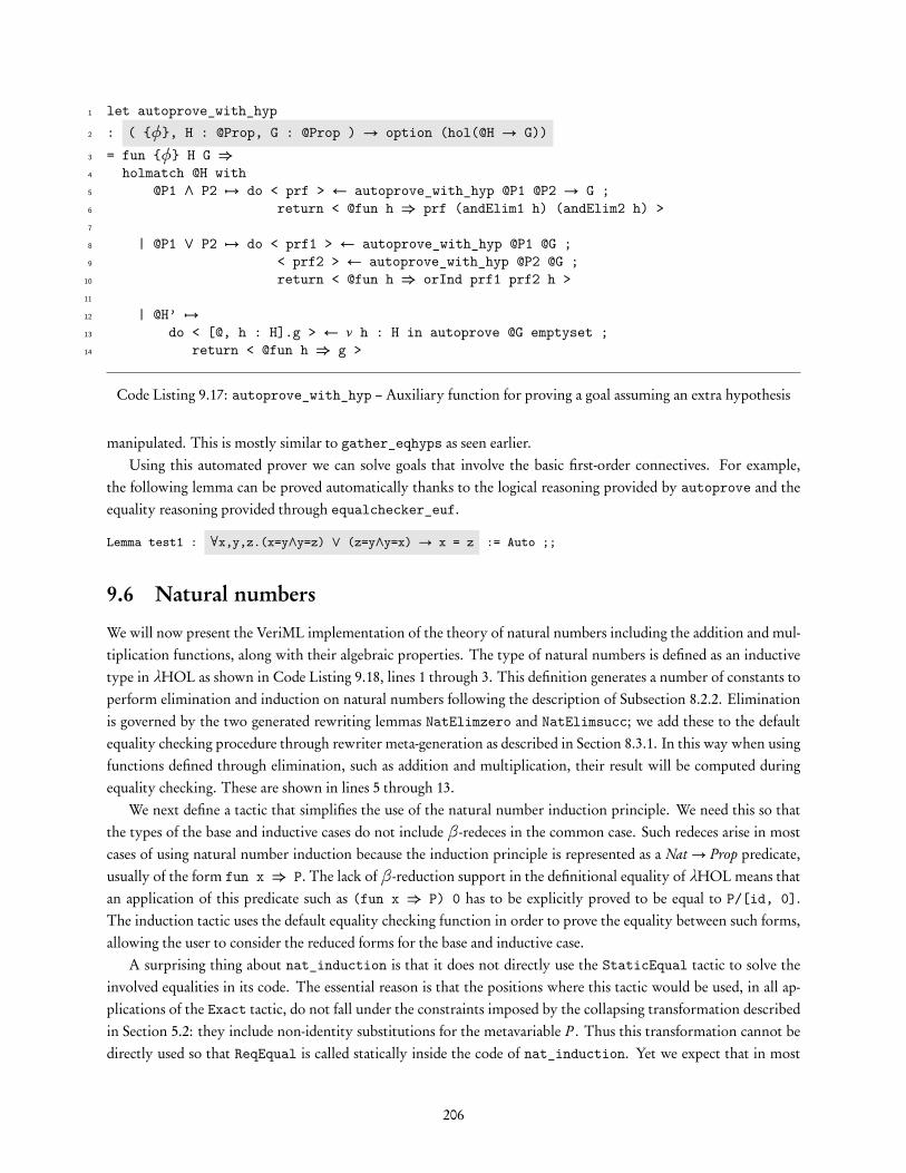
let autoprove_with_hyp1

: ( {φ}, H : @Prop, G : @Prop ) → option (hol(@H → G))2

= fun {φ} H G ⇒3

holmatch @H with4

@P1 ∧ P2 7→ do < prf > ← autoprove_with_hyp @P1 @P2 → G ;5

return < @fun h ⇒ prf (andElim1 h) (andElim2 h) >6

7

| @P1 ∨ P2 7→ do < prf1 > ← autoprove_with_hyp @P1 @G ;8

< prf2 > ← autoprove_with_hyp @P2 @G ;9

return < @fun h ⇒ orInd prf1 prf2 h >10

11

| @H’ 7→12

do < [@, h : H].g > ← ν h : H in autoprove @G emptyset ;13

return < @fun h ⇒ g >14

Code Listing 9.17: autoprove_with_hyp – Auxiliary function for proving a goal assuming an extra hypothesis

manipulated. This is mostly similar to gather_eqhyps as seen earlier.Using this automated prover we can solve goals that involve the basic first-order connectives. For example,

the following lemma can be proved automatically thanks to the logical reasoning provided by autoprove and theequality reasoning provided through equalchecker_euf.

Lemma test1 : ∀x,y,z.(x=y∧y=z) ∨ (z=y∧y=x) → x = z := Auto ;;

9.6 Natural numbers

We will now present the VeriML implementation of the theory of natural numbers including the addition and mul-tiplication functions, along with their algebraic properties. The type of natural numbers is defined as an inductivetype in λHOL as shown in Code Listing 9.18, lines 1 through 3. This definition generates a number of constants toperform elimination and induction on natural numbers following the description of Subsection 8.2.2. Eliminationis governed by the two generated rewriting lemmas NatElimzero and NatElimsucc; we add these to the defaultequality checking procedure through rewriter meta-generation as described in Section 8.3.1. In this way when usingfunctions defined through elimination, such as addition and multiplication, their result will be computed duringequality checking. These are shown in lines 5 through 13.

We next define a tactic that simplifies the use of the natural number induction principle. We need this so thatthe types of the base and inductive cases do not include β-redeces in the common case. Such redeces arise in mostcases of using natural number induction because the induction principle is represented as a Nat→ Prop predicate,usually of the form fun x ⇒ P. The lack ofβ-reduction support in the definitional equality of λHOL means thatan application of this predicate such as (fun x ⇒ P) 0 has to be explicitly proved to be equal to P/[id, 0].The induction tactic uses the default equality checking function in order to prove the equality between such forms,allowing the user to consider the reduced forms for the base and inductive case.

A surprising thing about nat_induction is that it does not directly use the StaticEqual tactic to solve theinvolved equalities in its code. The essential reason is that the positions where this tactic would be used, in all ap-plications of the Exact tactic, do not fall under the constraints imposed by the collapsing transformation describedin Section 5.2: they include non-identity substitutions for the metavariable P . Thus this transformation cannot bedirectly used so that ReqEqual is called statically inside the code of nat_induction. Yet we expect that in most

206

Inductive Nat : Type :=1

zero : Nat2

| succ : Nat → Nat ;;3

4

(* generated constants:5

NatElim : [T : Type]T → (Nat → T → T) → Nat → T;;6

NatElimzero : [T : Type]∀fz fs, NatElim fz fs zero = fz;;7

NatFoldsucc : [T : Type]∀fz fs n, NatElim fz fs (succ n) =8

fs n (NatElim fz fs n);;9

NatInd : ∀P : Nat → Prop, P zero → (∀n,P n → P (succ n)) → ∀n,P n;; *)10

11

global_rewriter_add (GenerateRewriter NatElimzero);;12

global_rewriter_add (GenerateRewriter NatElimsucc);;13

14

let nat_induction =15

fun φ (P : [φ, x : Nat].Prop)16

(pf1 : hol(@P/[id_φ,0]))17

(pf2 : hol(@∀x : Nat, P/[id_φ,x] → P/[id_φ, succ x]))18

(spf1 : hol(@?)) (spf2 : hol(@?)) (spf3 : hol(@?)) ⇒19

let < pf1’ > = Exact pf1 by spf1 in20

let < pf2’ > = Exact pf2 by spf2 in21

(Exact < @NatInd (fun x ⇒ P) pf1’ pf2’ > by spf3)22

: hol( @∀x : Nat, P ) ;;23

24

"NatInduction for x.P base case by e1 inductive case by e2" :=25

nat_induction @ (νx in @P) e1 e2 StaticEqual StaticEqual StaticEqual ;;26

Code Listing 9.18: Definition of natural numbers and natural induction tactic

207

cases where the induction tactic is used the constraints of the collapsing transformation will indeed be satisfied andthe involved proofs can be statically discovered at those points. We therefore transfer the requirement for the equal-ity proofs from the place where the induction tactic is defined to all the places where it is used. Through suitablesyntactic sugar, this additional requirement is hidden from the user.

In Code Listing 9.19, we present the definition and algebraic properties of the natural number addition function.The proofs of the properties are mostly automated save for having to specify the induction principle used. The factthat the induction principle has to be explicitly stated in full stems from a limitation in the type inference supportof the VeriML prototype. The automation comes from the extensible equality checking support: as soon as aproperty is proved it is added to the global default rewriter, which enables equality checking to prove the requiredobligations for further properties. Thus by proving the lemmas in the right order, we can limit the amount of therequired manual effort. After proving the commutativity and associativity properties of addition, we use a genericcommutativity and associativity equality module to add them to the global equality checking procedure. The typeof the generic module is:

equalchecker_comm_assoc : ({T : @Type}, {op : @T → T → T}) →(op_comm : @∀x y, op x y = op y x) →(op_assoc : @∀x y z,op x (op y z) = op (op x y) z) →equalchecker_t ;;

We do not give the code of this function here. It proceeds by pattern matching on terms, ordering applications of theop argument (here instantiated as the addition function plus), based on the hash values of their arguments. It yieldsa normalized form for terms that are equivalent up to associativity and commutativity. This function resembles thenaive equality rewriter of Section 9.3 and suffers from similar shortcomings: it can only prove simple cases whereassociativity and commutativity apply and it implements a very inefficient strategy.

The theory of multiplication is similar and is presented in Code Listing 9.20. We have elided the global rewriterregistration calls for presentation purposes; they directly follow the addition case. The main difference with additionis that not all proofs are automatic: in the theorems mult_x_Sy and mult_plus_distr, the equality checkingsupport is not enough to prove the inductive case. We have to specify explicitly that terms should be rewrittenbased on the induction hypothesis instead – using a tactic similar to the naive rewriter of Section 9.3, which onlyrewrites terms based on a given equality proof. To see why this is necessary, consider the following proof obligationfrom mult_x_Sy, line 17:

I H : z ∗ (succ y) = z +(z ∗ y)

G : (succ z) ∗ (succ y) = (succ z)+ ((succ z) ∗ y)

Equality checking proceeds as follows. First we rewrite the left-hand side and right-hand side of the equality tonormal form based on the current default rewriter:

(LHS) (succ z) ∗ (succ y)−→ (mult_Sx_y)

(succ y)+ z ∗ (succ y)−→ (plus_Sx_y)

succ (y + z ∗ (succ y))

(RHS) (succ z)+ ((succ z) ∗ y)−→ (plus_Sx_y)

succ (z +(succ z) ∗ y)−→ (mult_Sx_y)

succ (z + y + z ∗ y)

The current equality checking cannot decide these two normal forms to be equal. In order for the EUF procedureto take the induction hypothesis into account, there would need to be an explicit z + z ∗ y subterm in the RHS.Such a term would only appear if we rewrite the RHS into y + z + z ∗ y based on commutativity, yet the naivecommutativity support does not have any sophistication so as to perform this commutativity step; rewriting intothis form would be just a coincidence based on the hash values of the terms and we should not therefore depend on

208

Definition plus : Nat → Nat → Nat := fun x : Nat ⇒ fun y : Nat ⇒1

NatElim y (fun p r ⇒ succ r) x ;;2

3

Temporary Rewriter (Unfolder plus) in {4

Theorem plus_Z_y : ∀y,0 + y = y := Auto ;;5

Theorem plus_Sx_y : ∀x y,(succ x) + y = succ (x + y) := Auto ;;6

}7

8

global_rewriter_add (GenerateRewriter plus_Z_y);;9

global_rewriter_add (GenerateRewriter plus_Sx_y);;10

11

Theorem plus_x_Z : ∀x : Nat, x + 0 = x :=12

NatInduction for x. x + 0 = x13

base case by Auto14

inductive case by Auto ;;15

16

Theorem plus_x_Sy : ∀(x y : Nat), x + (succ y) = succ (x + y) :=17

Intro x y in18

Instantiate19

(NatInduction for z. z + (succ y) = succ (z + y)20

base case by Auto21

inductive case by Auto)22

with @x ;;23

24

global_rewriter_add (GenerateRewriter plus_x_Z);;25

global_rewriter_add (GenerateRewriter plus_x_Sy);;26

27

Theorem plus_comm : ∀(x y : Nat), x + y = y + x :=28

Intro x y in29

NatInduction for y. x + y = y + x30

base case by Auto31


33

Theorem plus_assoc : ∀(x y z : Nat), x + (y + z) = (x + y) + z :=34

Intro x y in35

NatInduction for z.x + (y + z) = (x + y) + z36

base case by Auto37


39

global_equalchecker_add (equalchecker_comm_assoc plus_comm plus_assoc) ;;40

Code Listing 9.19: Addition for natural numbers

209

Definition mult : Nat → Nat → Nat := fun x : Nat ⇒ fun y : Nat ⇒1

NatElim 0 (fun p r ⇒ y + r) x ;;2

3

Theorem mult_z_y : ∀y : Nat, 0 * y = 0 := Auto ;;4

Theorem mult_Sx_y : ∀(x y : Nat), (succ x) * y = y + (x * y) := Auto ;;5

6

Theorem mult_x_z : ∀x : Nat, x * 0 = 0 :=7

NatInduction for x. x * 0 = 08

base case by Auto9


11

Theorem mult_x_Sy : ∀x y, x * (succ y) = x + (x * y) :=12

Intro x y in13

Instantiate14

(NatInduction for z. z * (succ y) = z + (z * y)15

base case by Auto16

inductive case by ( Intro z in Assume IH in Rewrite @IH in17

Auto ) )18

with @x ;;19

20

Theorem mult_comm : ∀x y, x * y = y * x :=21

Intro x in22

NatInduction for y. x * y = y * x23

base case by Auto24


26

Theorem mult_plus_distr : ∀x y z, x * (y + z) = (x * y) + (x * z) :=27

Intro x y z in28

Instantiate29

(NatInduction for a. a * (y + z) = (a * y) + (a * z)30

base case by Auto31

inductive case by ( Intro a in Assume IH in Rewrite @IH in32

Auto ) )33

with @x ;;34

35

Theorem mult_assoc : ∀x y z, x * (y * z) = (x * y) * z :=36

Intro x y in37

NatInduction for z.x * (y * z) = (x * y) * z38

base case by Auto39


Code Listing 9.20: Multiplication for natural numbers

210

it. What we do instead is to force a rewriting step in the LHS based on the inductive hypothesis, resulting in theequivalent term succ (y+ z+ z ∗y). Now the naive commutativity support will rewrite both the LHS and RHS intothe same normal form and syntactic equality yields the desired equality proof.

The distributivity property of multiplication with regards to addition requires no special provision in terms ofequality checking support; the default meta-generated rewriter for it is enough to handle cases where it needs to beused.

9.7 Normalizing natural number expressions

We will now develop a more sophisticated rewriter that normalizes arithmetic terms up to associativity and com-mutativity of addition and multiplication. The rewriter works as follows: given an arithmetic term, it constructsa list of monomials of the form a · x where a is a constant expression and x is a variable or a product of vari-ables (nat_to_monolist in Code Listing 9.23); the list is sorted so that monomials on the same variable be-come adjacent (sort_list in Code Listing 9.22); consecutive monomials on the same variable are factorized(factorize_monolist in Code Listing 9.24); and the list of monomials is converted back into an arithmetic expres-sion. These auxiliary functions need to be partially correct so that the resulting rewriter can prove that rewriting aterm t to t ′ based on this sequence of steps is actually valid. For example, the nat_to_monolist function has toreturn a monomials list that, when summed, is equivalent to the original number; and sorting a list of monomialsneeds to return the same list, albeit permuted. Note that the second property of sorting, namely the fact that thereturned list is ordered, is not important for our purposes.

In order to be able to specify and reason about the behavior of these functions, we need a definition of lists atthe level of the logic. This is shown in Code Listing 9.21. Contrast this definition with the definition of lists at thecomputational level of VeriML, as seen earlier in Code Listing 9.1: the logic definition allows us to reason aboutlists, describing the behavior of list-related functions at the logic or computational level; whereas the computationaldefinition allows us to define lists of arbitrary VeriML values, including mutable references and contextual terms butprecludes reasoning about their behavior. The effort associated with having to duplicate definitions can be mitigatedby having logic definitions implicitly define the equivalent computational versions as well.

In Code Listing 9.21 we also give the definitions of the append function at the logical level and of sumlist

which accumulates together the members of lists of natural numbers. We also define the predicate of a list being apermutation of another, as well as the auxiliary predicate removed l1 elm l1’. This stands for the property “ifthe element elm is removed from the list l1, the resulting list is l1’”. Last, we give statements of lemmas about theinteraction of these functions. We do not give the proofs here; these follow the ideas presented so far. The proofthat presents the most difficulty is the permutation_symm theorem, taking 50 lines in total. It requires proving aninversion lemma for permutations and a number of manual proof steps. This proof could be significantly improvedby meta-generation of inversion principles, as well as the development of automation for user-defined predicatesfollowing the ideas presented for the equality predicate; we leave these matters to future work.

In Code Listing 9.22 we present the sorting function for lists. This is a computational function that manipulateslogical lists. The reason behind this choice is that we want to sort lists based on the hash of their elements – that is,based on an extra-logical operation –, yet we also need a proof that sorting returns a permutation of the original list– therefore the choice of logical lists. We leave the comparison operation as a parameter to the sorting function. Thesorting algorithm we implement is selection sort; we use the auxiliary function min_list to remove the minimumelement of a list. In both functions we provide manual proofs of most obligations, using the definitions and lemmasof Code Listing 9.21. A point worth mentioning is that we need to explicitly rewrite the input lists to head-normal

211

Inductive List [ T : Type ] : Type :=1

nil : List2

| cons : T → List → List ;;3

4

Definition append [T : Type] : List/[T] → List/[T] → List/[T] :=5

fun x y ⇒ ListElim y (fun hd tl r ⇒ cons hd r) x ;;6

7

Definition sumlist : List/[Nat] → Nat :=8

ListElim 0 (fun hd tl r ⇒ hd + res) ;;9

10

Lemma sum_append : ∀l1 l2,11

sumlist (append l1 l2) = (sumlist l1) + (sumlist l2)12

13

Inductive removed [T : Type] : List/[T] → T → List/[T] → Prop :=14

removedHead : ∀hd tl, removed (cons hd tl) hd tl15

| removedTail : ∀elm hd tl tl’, removed tl elm tl’ →16

removed (cons hd tl) elm (cons hd tl’) ;;17

18

Lemma removed_sum : ∀l elm l’,19

removed l elm l’ → sumlist l = elm + (sumlist l’)20

21

Inductive permutation [T : Type] : List/[T] → List/[T] → Prop :=22

permutationNil : permutation nil nil23

| permutationCons : ∀hd l1’ l2 l2’, removed l2 hd l2’ →24

permutation l1’ l2’ →25

permutation (cons hd l1’) l2 ;;26

27

Theorem permutation_sum : ∀l1 l2,28

permutation l1 l2 → sumlist l1 = sumlist l229

30

Lemma permutation_removed [T : Type] : ∀l1 elm l1’ l2’,31

removed l1 elm l1’ → permutation l1’ l2’ →32

permutation l1 (cons elm l2’)33

34

Theorem permutation_symm [T : Type] : ∀l1 l2,35

permutation l1 l2 → permutation l2 l136

Code Listing 9.21: Definition of lists and permutations in λHOL, with associated theorems

212

letrec min_list1

: ({φ : ctx}, {T : @Type}, cmp : (@T) → (@T) → bool, l : @List) →2

(min : @T) × (rest : @List) × hol(@removed l min rest)3

= fun {φ T} cmp l ⇒4

let < @l’ , @pfl’ > = default_rewriter @l in5

let < @min, @rest, @pf > =6

holmatch @l’ with7

@nil 7→ error8

| @cons hd nil 7→ < @hd , @nil , @removedHead ? ? >9

| @cons hd tl 7→10

let < min’, rem, pf > = min_list cmp @tl in11

if (cmp @hd @min’ ) then12

< @hd , @tl, Exact @removedHead hd tl >13

else14

< @min’, @cons hd rem, @removedTail pf >15

in < @min , @rest , {{ Auto }} > ;;16

17

18

let sort_list19

: ({φ : ctx}, {T : @Type}, cmp : (@T) → (@T) → bool, l : @List) →20

(l’ : @List) × hol (@permutation l l’)21

= fun {φ T} cmp l ⇒22

let < lnorm , pflnorm > = default_rewriter @l in23

let < l’ , pfl’ , u > =24

holmatch @lnorm with25

@nil 7→ < @nil , @permutationNil >26

| @cons hd tl 7→27

let < newhd, newtl, prf1 > = min_list cmp (@cons hd tl) in28

let < newtl’, prf2 > = sort_list cmp @newtl in29

let < prf2’ > = < @permutation_symm prf2 > in30

< @cons newhd newtl’ ,31

@permutation_symm (permutationCons prf1 prf2’) >32

in < @l’, {{ Auto }} > ;;33

Code Listing 9.22: Selection sorting for lists

213

let factorize_monolist1

: ({φ : ctx}, l : @List) → (l’ : @List) × hol( @sumlist l = sumlist l’ )2

= fun {φ n} l ⇒ holmatch @l with3

@cons (hda * hdb) tl 7→4

let < tl’ , pftl’ > = factorize_monolist @tl in5

holmatch @tl’ with6

@cons (hdc * hdb) tl’’ 7→7

< @cons ((hda + hdc) * hdb) tl’’ ,8

{{ Rewrite @pftl’ in ReqEqual }} >9

| @tl’ 7→ < @cons (hda * hdb) tl’ , StaticEqual >10

| @l 7→ < @l , StaticEqual > ;;11

12

let rewriter_arithsimpl : rewriter_module_t =13


holmatch @e with15

@e1 + e2 7→16

let < l0, pf1 > = nat_to_monolist @e1+e2 in17

let < l1, pf2 > = sort_list cmp @l0 in18

let < l2, pf3 > = factorize_monolist @l1 in19

< @sumlist l2, {{ Cut @permutation_sum l0 l1 in Auto }} >20

| @e 7→ < @e , StaticEqual > ;;21

Code Listing 9.24: Rewriter module for arithmetic simplification (2/2)

form before pattern matching is performed, as matching happens only up to syntax and not up to β-equivalence orevaluation of logical functions such as append.

The rest of the code for arithmetic simplifications is presented in Code Listing 9.23 and 9.24, following thedescription given earlier. Sorting of monomial lists is done using the comparison function cmp. This functiononly uses the hash value of the variable component x, thus making monomials on the same variable adjacent in thesorted list. It is worth noting that most of the proof obligations for these functions are solved automatically for themost part –an additional hint is required in some cases– and are validated statically following the ideas we have seenearlier.

9.8 Evaluation

This concludes our presentation of the examples we have implemented in VeriML. It is worth noting that the fullcode of the examples mentioned above is about 1.5k lines of VeriML code, including all the infrastructure and basiclibrary code we describe. We offer a breakdown of the line counts for the different modules in Table 9.1. In thesame table we note the line counts for the proof-related aspects of the code, which include all logic definitions,proofs, hints (as additions of meta-generated rewriters) and induction tactics, in order to give an accurate portrayalof the λHOL-related reasoning that the programmer has to do. It is worth noting that the vast majority of theproof-related code corresponds to defining and proving the theory of natural numbers, lists and permutations. Theactual conversion implementation functions have minimal manual proof involved.

It is worth contrasting these line counts with the two tactics in Coq that are roughly equivalent in function-ality to our implementation of the EUF and arithmetic simplification conversion rules, namely congruence andring_simplify respectively. This comparison is shown in Table 9.2. For EUF conversion in VeriML, we have in-cluded the naive equality rewriter as well as the main EUF module; for arithmetic simplification, we have included

215

Logic definitions,Total lines of code proofs, hints

Basic library 131 16Basic connectives 36 36Basic rewriting support 191 19Naive equality rewriter 79 2Hash tables and sets (Prop and Type) 69x2=138 0EUF rewriter 200 0β-rewriting 21 1Auto prover 178 14Naive comm./assoc. rewriting 111 17Force rewriting on hypothesis 56 7Theory of natural numbers 128 128Lists, permutations and sorting 200 158Arithmetic simplification 84 3

Full code involved 1581 401

Table 9.1: Line counts for code implemented in VeriML

Total code Manual proofVeriMLEUF conversion 279 2Arithmetic simplification 395 178Natural numbers theory 128 128

CoqCongruence 1437 62Ring simplification 1997 846Abstract ring theory 259 259

Table 9.2: Comparison of line counts for EUF rewriting and arithmetic simplification between VeriML and Coq

216

the naive commutativity and associativity rewriter, the theory of lists and the arithmetic simplification procedure.In both of these cases some of the code is reusable: e.g. the theory of lists consists of theorems that are usefulindependently of arithmetic simplification, and the code of the naive rewriter is mostly reused for implementingthe forced rewriting procedure. In computing the line counts for the Coq versions, we have manually isolated theproof-related lines, such as calls to tactics and CIC constructors inside ML code in the case of the congruence tactic,and the lemmas proved using LTac proof scripts in the case of ring simplification. In the same table, we have alsoincluded the counts for our development of the theory of natural numbers, as well as the theory of abstract ringsused by ring_simplify which are composed of roughly the same theorems.

The VeriML versions of the tactics and proofs compare favorably to their Coq counterparts; it is telling thatthe manual proofs required for all of our VeriML code, including basic logic definitions and tactics, is half the sizeof the proofs required just for arithmetic simplification in Coq. In arithmetic simplification, the Coq proofs areabout 5 times larger than their VeriML equivalent; in the EUF procedure, the ratio is 30:1, or 3:1 if we include thebasic rewriting support code of VeriML (which is what accounts for the congruence properties). The main reasonbehind the significant reduction in manual proof size for the VeriML versions is the way we implement our proofsand proof-producing functions, making use of the extensible conversion support. As for the overall reduction incode size, the main reason is that we do not have to go through encodings of logical terms such as the ones usedby proof-by-reflection or translation validation, as required by the Coq versions, but can rather work on the exactterms themselves. Of course the comparison of line counts for the programming aspect of the procedures cannotprovide accurate grounds for drawing conclusions. This is especially true since the compared tactics are for differentlogics, use more realistic and full-featured implementations of the algorithms we describe (e.g. congruence takesinjectivity of constructors into account) and the performance is not yet comparable, owing largely to our prototypeVeriML implementation. Still, the difference in manual proof effort required indicates the savings that VeriML canoffer.

217

Chapter 10

Related work

There is a large body of existing related literature that the work in this dissertation rests upon. The design ofVeriML is such that it can be viewed as either a programming language tailored to tactic programming or as acomplete proof assistant. We will therefore compare VeriML to other tactic development methodologies as well asexisting architectures of proof assistants. When viewed as a programming language, the core departure of VeriMLfrom traditional functional programming languages such as ML and Haskell is the availability of constructs fortype-safe manipulation of an object language; we will present a number of existing language designs that containsimilar constructs. Last, VeriML represents a particular way of combining a logic with a side-effectful programminglanguage, where a strong separation between the two languages is maintained. We will compare this approach withother potential combinations.

10.1 Development of tactics and proof automation

Tactic development in ML. Most modern proof assistants, such as HOL [Slind and Norrish, 2008, Harrison,1996], Isabelle [Paulson, 1994], Coq [Barras et al., 2012] and NuPRL [Allen et al., 2000], allow users to extendthe set of available tactics, by programming new tactics inside the implementation language of the proof assistant.In all cases this language is a dialect of Standard ML [Milner, 1997]. In fact, ML was designed precisely for thispurpose in the context of the original LCF system [Gordon et al., 1979] – as the Meta Language of the system,used to manipulate the terms of the logic – the object language. Developing tactics in ML is thus the canonicalmethodology used in the direct descendants of this system such as HOL.

The programming constructs available in ML were chosen specifically with tactic development in mind, makingthe language well-suited to that purpose. For example, higher-order functions are available so that we can definetacticals – functions that combine other tactics (which are functions themselves). The programming model availablein ML is very expressive, allowing general recursion, mutable references and other side-effectful operations; thisenables the development of efficient tactics that make use of sophisticated algorithms and data structures such asdiscrimination nets [Gordon, 2000].

The main problem with tactic development in ML is that it is essentially untyped. Logical terms and proofs areencoded within ML as algebraic data types. Data types are simply-typed in ML, effectively identifying all proofsand all terms at the level of types and precluding any extra information – such as the context of free variablesthey depend on, or the kinds of terms, or the consequence of proofs – from being available statically. This hurtsthe composability of tactics and their maintainability as well, as we cannot give precise signatures to the kinds of

218

arguments they expect, the results they produce and the relationships between them. VeriML can be viewed as adependently-typed extension of ML that addresses this shortcoming, by making the type of proofs and logical termsdependent on the information produced by the type system of the logic. The relationship between programmingtactics in VeriML instead of ML is therefore similar to the relationship of developing functional programs in MLinstead of Lisp.

For example, the VeriML type we gave to rewriters is the following:

(φ : ctx,T : Type, t : T )→ (t ′ : T )× (t = t ′)

In ML, the equivalent type would be:

holterm→ holterm× holproof

In this type, the fact that the input and output terms share the same type and variable context, as well as the factthat the output proof witnesses the equivalence between the input and output terms is lost. Still, the types holterm

and holproof have equivalent types in VeriML, constructed by hiding the extra context and typing informationthrough existential packages: the types (φ : ctx,T : Type)× (t : T ) and (φ : ctx, P : Prop)× (p : P ), respectively.This shows that, in principle, any tactic written in ML for an LCF-style proof assistant can be written as a VeriMLfunction instead.

Another shortcoming of ML in terms of tactic development is that users have to master the internal represen-tation of logical terms and proofs in the proof assistant. For examples, the user needs to know the details of howlogical variables are encoded through deBruijn indices in order to develop tactics that deal with open terms. Thiscan be somewhat mitigated through proper syntactic extensions to ML as done in HOL-Light [Harrison, 1996].The first-class constructs for pattern matching over open logical terms and contexts make tactic development inVeriML more convenient, hiding the implementation details of the proof assistant.

Tactic development in LTac. The Coq proof assistant offers the higher-level LTac language [Delahaye, 2000,2002], which is specifically designed for tactic development. This is a significant feature, as it enables users to extendthe provided automation with their own tactics through convenient pattern-matching constructs, addressing theabove-mentioned shortcoming of tactic development in ML. LTac has been put to good use in various developmentswhere the manual proof effort required is reduced to a minimum [e.g. Chlipala, 2011, Morrisett et al., 2012]. Thekey construct of LTac is the support for pattern matching on proof states with backtracking. It is used to examinethe forms of the current hypotheses and the current goal and to issue the corresponding tactics; upon failure of suchtactics, LTac implicitly backtracks to an alternative pattern matching case allowing further progress. The patternmatching construct of VeriML has been influenced by LTac; it is similar in features, save for the backtrackingsupport which we have chosen to leave as a user-defined feature instead.

Other than the pattern matching construct, LTac is an untyped functional language without support for ML-style data types or side-effects such as mutability. This hurts expressivity, prompting users to use ad-hoc idioms toovercome the limited programming model of LTac. In order to write more sophisticated tactics such as congruenceclosure, one has to revert to ML. Also, LTac is interpreted, leading to long running times for large tactics. Last,the untyped nature of the language makes LTac tactics notoriously hard to maintain and debug and are sometimesavoided precisely for this reason [e.g. Nanevski et al., 2010]. VeriML addresses these shortcomings by offering anexpressive type system, a full programming model and compilation through translation to ML; it can thus be seenas a ‘typed LTac’.

219

Proof by reflection. Coq offers another methodology for writing user-defined tactics, enabled by the inclusion ofthe conversion rule in its logic. This rule renders the logic (referred to as Gallina) into a functional programminglanguage. For reasons of soundness, programs in this language need to be terminating. Through the techniqueof proof by (computational) reflection [Boutin, 1997], we can program the decision procedures directly in the logiclanguage. The technique consists of reflecting part of the propositions of the logic as an inductive type within thelogic itself, so that they can be manipulated as a normal datatype. Also, we need to define encoding and decodingfunctions from propositions to the inductive type and back. The decision procedure can then be programmed asa function at the level of the logic and its correctness can be stated and proved as a normal theorem, using theinteractivity support of Coq. A sketch of the different components involved in the proof-by-reflection approachwould be as follows using VeriML-style types:

Inductive IProp : Type := IAnd ip1 ip2 | IOr ip1 ip2 | · · · .encode : Prop→ IProp (programmed in LTac)decode : IProp→ Prop (programmed in Gallina)decision_procedure : IProp→ Bool (programmed in Gallina)correctness : ∀ i p : IProp.decision_procedure i p = true→ decode i p

In VeriML, the first three components would not be needed because we can manipulate propositions directly; andwe can write a single function that combines the last two components:

decision_procedure : (P : Prop)→ option (P )

The fact that the decision procedures written in proof-by-reflection style are certified means that the proceduresdo not need to generate proof objects; thus procedures written in this style are very efficient. Together with thefact that Gallina functions are total, decision procedures that are complete for certain theories do not even needto be evaluated; their definition and soundness proof is enough to prove all related theorems directly. This fact hasprompted Pollack [1995] to propose total and certified decision procedures, developed using a mechanism similar toproof-by-reflection, as the main extensibility mechanism for proof assistants; yet this proposal has not been followedthrough.

The main problem with this approach is that it has a high up-front cost for setting up the reflection, especiallyif we want our decision procedure to manipulate open terms: a concrete deBruijn representation must be used forrepresenting variables and the user must also develop functions to manipulate this representation. Pattern matchingover such encodings is cumbersome compared to the first-class constructs offered by LTac or VeriML. Also, theprogramming model of Gallina does not support side-effects in the code of the decision procedures. In VeriMLwe can code similar procedures which are also certified, yet the total correctness requirement is relaxed: VeriMLprocedures can still fail to terminate successfully, so they need to be evaluated to completion. This is a limitationcompared to proof-by-reflection, as it increases the required run time; but it can also be viewed as an advantage,as we do not have to prove termination of the decision procedures. Non-terminating behavior is not necessarilya problem and can be used towards good effect in our developments (e.g. consider the naive equality rewriter ofSection 9.3, which is non-terminating in some cases). In other cases, a procedure is terminating yet its terminationcriterion might be difficult to prove. In proof-by-reflection, the totality requirement has to be circumvented throughthe use of an argument that limits the amount of steps that are performed. Also, the certification of VeriMLprocedures is more light-weight than proof by reflection: the type system of VeriML can be viewed itself as a light-weight certification mechanism. Coupled with the support for static proof expressions to solve the required proofobligations inside procedures, this significantly limits the manual proof effort required.

Still, the proof-by-reflection technique can be used in the context of VeriML, which could potentially be useful inlarge developments. In fact VeriML offers benefits for programming the LTac components of the proof-by-reflection

220

procedures. For example, we could assign the following rich type to the encoding function:

encode : (P : Prop)→ (I : IProp)× (decode I = P)

Also, the small-scale automation mechanism used to implement proof-by-reflection, namely the conversion rule, isprogrammed directly in VeriML as well, leading to a smaller trusted base.

Yet the unique characteristic of the proof-by-reflection approach is that the tactics are themselves logical func-tions. Therefore we can reason about them using the full features of the logic, allowing us to prove deep theoremsabout their behavior. Together with the fact that Gallina has an infinite type hierarchy with computation allowed atany level, this would allow us to give very precise signatures to tactics – e.g. capturing precisely the set of cases wherean automation tactic can be applied successfully. In contrast, VeriML maintains a two-layer architecture, where tac-tics are written in the computational language and cannot be reasoned about in the logic. Thus the signatures thatwe can give to tactics are limited to what is allowed by the VeriML type system. In the future we would like to ex-plore the potential of offering VeriML as a surface language in a proof assistant such as Coq, where VeriML-definedtactics are compiled down to Gallina tactics through proof-by-reflection. This is an interesting alternative that offerssome of the benefits of both approaches: the up-front cost of setting up proof-by-reflection would be significantlyreduced, but we could also reason about VeriML tactics in the logic. Still, the tactics would not be able to use side-effects and an efficient evaluation strategy for the conversion rule (e.g. compilation-based) would need to be part ofthe trusted base of the system.

Unification-based automation. Coq includes another small-scale automation mechanism other than the conver-sion rule: a unification-based type inference engine used to elaborate surface-level terms to concrete CIC terms. Byissuing hints to this engine, users can perform automation steps as part of type inferencing. The hints take the formof Prolog-like logic programs. Gonthier et al. [2011] show how these hints can be encoded through the existing Coqmechanism of canonical structures (a generalization of type classes); also, the experimental Matita proof assistantincludes explicit support for these unification hints [Asperti et al., 2009]. This technique offers various advantagesover untyped LTac-style automation tactics: Automation procedures are essentially lemmas whose premises aretransparently resolved through unification. Therefore we can specify and develop the main part of the automationlemmas by using the existing infrastructure of the proof assistant for proving lemmas. Also, since the technique isbased on a small-scale automation mechanism, automation developed in this way applies transparently to the user,allowing us to omit unnecessary details.

The limitations of this approach are that automation procedures need to be written in the logic programmingstyle instead of a more natural functional programming model. Also, procedures written in this way are hard todebug, as missing or erroneous hints can result in unspecified behavior depending on how the type inferencingengine works. Also the support for writing this style of procedures in Coq is still rudimentary and requires ad-hoc usage patterns and a high up-front cost. Our approach to extensible small-scale automation allows for moresophisticated procedures that use a full programming model. Still, the unification-based approach is useful in casesother than proof automation, such as automatic instantiation of generic mathematical operators. We have not yetprogrammed a unification algorithm as a VeriML procedure; doing so in the future will allow us to replicate thistechnique in the context of VeriML.

A calculus of tactics. An alternative tactic development methodology is described by Jojgov and Geuvers [2004],where a calculus of basic building blocks for writing tactics is presented. The calculus is based around an extensionof λHOL with metavariables presented in Geuvers and Jojgov [2002], similar to our own extensions of λHOL.Though the provided building blocks do not allow the same generality as the full ML programming model we

221

support, they include an explicit unification construct between terms that both contain metavariables. This isa more general construct than the pattern matching supported in VeriML, where only the patterns can containmetavariables and the scrutinees must be closed. Extending our language so that such a unification construct can bebuilt-in or programmed within the language is a high priority for future development of VeriML.

Automation tactics with user-defined hints. A last way that user-defined automation is added in current proofassistants is to use automated tactics that implement a fixed proof search strategy, but can be informed through user-defined hints. Though this is not a tactic development technique per se, it is relevant here since adding user-definedautomation is one of the main reasons why tactic development is important. There are multiple instances of thistechnique in a wide variety of current proof assistants.

First, the Isabelle simplifier [Paulson, 1994, Nipkow et al., 2002] is one such case: the simplifier is a powerfulrewriting-based prover that is used in most tactics and can be informed through user-defined rewriting lemmas.Users can register first-order lemmas they prove directly with the simplifier, increasing the available automation.This mechanism is quite similar in function to our extensible equality checking support, though it applies morewidely – owing both to properties of the logic (propositional equality coincides with propositional equivalence)and to more sophisticated infrastructure for the simplifier (e.g. rewriting lemmas can include premises). Still, ourequality checking allows more sophisticated extensions that are not possible for the Isabelle simplifier: we canextend it not only with first-order lemmas, but with arbitrary decision procedures as well, written in a general-purpose programming model. For example, the congruence closure function for equality hypotheses we supportcannot be directly added to the simplifier.

Another instance of this technique that is often used as part of large proof developments is to use a powerfuluser-defined automation tactic that is informed of domain-specific knowledge through user-provided hints [e.g.Chlipala, 2008, 2011, Morrisett et al., 2012]. The hints can be as simple as a rewriting lemma and as complicated asan LTac tactic that is to be applied for specific propositions. We refer to this technique as adaptive proof scripts.By replacing proof scripts with a single call to the automation tactic, our proofs can adapt to changes and additionsin our definitions: if the changes are small, automation will still be able to find a proof and the proof scripts willgo through; larger changes will make automation fail, but users can respond to the points of failure by addingappropriate lemmas and tactics as hints. This approach has inspired the way that we program and use equalitychecking to provide automation to other tactics. The extensions that we add to the equality checking procedure canbe seen as a form of adding sophisticated user hints.

A last instance of this technique is the standard way of developing proofs in fully automated provers such asACL2 [Kaufmann and Strother Moore, 1996] and SMT solvers [e.g. De Moura and Bjørner, 2008]. Lemmas thathave already been proved play implicitly the role of hints. By offering very sophisticated and efficient proof searchalgorithms, such provers can handle large theorems automatically, with a small number of additional auxiliarylemmas. Still, these provers offer poor or no support for extensibility with user-defined tactics; this limits theirapplicability in cases where the fixed proof search algorithms available are not well-suited to the user domain.

In all such cases, the basic automation tactic can be viewed as a small-scale automation mechanism, as it is usedubiquitously and transparently throughout the proof. It is also extensible, owing to the support for user-definedhints. This extensibility is key to the success of such techniques, allowing users to omit a large amount of details;it has directly inspired our focus on offering extensible small-scale automation mechanisms. VeriML is a goodcandidate as the implementation language of such automation tactics, especially compared to LTac or proof byreflection: other than the benefits we have discussed already, it allows the use of hash tables and other efficient datastructures in order to represent the database of user-supplied hints.

222

Overall, VeriML offers a single language that combines many of the benefits of these existing approaches. Develop-ing tactics in VeriML is the only methodology among the ones presented above that combines three characteristics:

1. expressivity, where a full, side-effectful programming model is available for writing sophisticated tactics;

2. convenience, where first-class constructs for pattern matching on arbitrary open logical terms and proof statesare available; and

3. safety, where the behavior of tactics can be specified and checked through a type system, enabling increasedstatic guarantees as well as better maintainability and composability.

Also, we have shown how many of the techniques mentioned above can be programmed directly within VeriML.Last, it is important to stress the fact that users only have to master a single language and a single programmingmodel. In many current developments, the above techniques are combined in order to get the automation behaviorrequired as well as good efficiency. The fact that VeriML is compiled and does not need to produce proof objectsshows that similar efficiency can be achieved in the future using a single language.

10.2 Proof assistant architecture

The LCF family of proof assistants has had a profound influence on the design of VeriML. The main shared char-acteristic with VeriML is that these proof assistants follow the language-based approach: all aspects of the proofassistant, including the basic tactics, decision procedures and equality checking functions, as well as user-developedproofs and proof-producing functions, are implemented within the same language, namely ML. In the LCF family,the core logic implementation is offered as an ML module that introduces two abstract data types: a type of log-ical terms such as propositions and domain objects (the holterm type as mentioned above) and a type of proofs(holproof). The only way to produce values of such types is through the constructor functions offered by thismodule. These constructors are in one-to-one correspondence with the logical rules, guaranteeing that all values ofthe proof type correspond to a particular derivation in the logic. Also, basic destructor functions for looking intothe structure of logical terms are offered. This design leads to an extensible proof assistant that is conceptually clearand easy to master. It allows the use of the full ML programming model when writing proof-producing functions.Thanks to the LCF design and to the type safety property of ML, full proof objects do not need to be producedto guarantee validity. The same property is true in VeriML, as shown in the proof erasure corollary of type safety.VeriML can be viewed as following precisely the same architecture, albeit with a significant departure: the basic con-structor and destructor functions are dependently-typed instead of simply-typed, capturing the context and typinginformation from the logic type system. The correspondence is direct if we consider the pattern matching supportas a principled way to offer typed destructors over logical terms.

More recently, proof assistants based on a two-layer architecture such as Isabelle and Coq have become popular.In these, a higher-level language is made available to users for developing proofs, different from the implementationlanguage of the proof assistant. This allows increased interactivity support, convenient syntax for writing proofs andin the case of Coq/LTac, a higher-level language for tactic development. Despite the benefits that this architectureoffers, it has a significant downside: user-defined tactic development is de-emphasized and the programming modelavailable for user-defined tactics is significantly limited compared to ML. The Coq architecture departs from LCFin another significant way: the LCF approach to hiding the data types of the logic is not followed, and tactics needto construct full proof objects to be checked by a proof checker. This leads to significant scalability issues in large

223

developments, which are usually mitigated through increased use of proof-by-reflection. The VeriML design allowsincreased interactivity through queries to the type checking engine; supports convenient tactic syntax throughsyntactic sugar extensions as presented in Chapter 9; maintains the language-centric approach of the original LCFdesign; and allows users to control the size of proof objects through selective use of the proof erasure semantics.

The ACL2 theorem prover [Kaufmann and Strother Moore, 1996] is an interactive proof assistant that followsa very different style than the LCF-based or LCF-derived proof assistants we have presented so far. It is based on asimple first-order logic and eschews the use of tactics, opting instead to use a powerful automated theorem proverbased on rewriting that takes into account user-defined rewriting lemmas. The increased automation is in largemade possible by the simplicity of the logic language and the use of domain-specific decision procedures. ACL2 hassuccessfully been used for large-scale verification of software [e.g. Bevier et al., 1987, Young, 1989] and hardware[e.g. Brock et al., 1996], which shows that rewriting-based proving can be expressive and powerful. We would liketo investigate the addition of ACL2-like proving in our extensible rewriting infrastructure in the future. Extensionsto the existing rewriters in ACL2 are made in the form of metafunctions; yet the untyped nature of ACL2 doesnot allow metafunctions to use facts that can be discovered through the existing rewriters [Hunt et al., 2005]. TheVeriML type system addresses this shortcoming.

In the traditional ACL2 system the proofs are not foundational and one needs to trust the entirety of the systemin order to trust their validity. Milawa [Davis, 2010] is a theorem prover that addresses this shortcoming of ACL2.It is based on a similar first-order logic which includes a notion of proof objects. A checker for this logic constitutesthe first level of the Milawa system. More sophisticated checkers are then developed and proved sound within thesame logic using a technique similar to proof-by-reflection as presented above. In this way, a large number of theoriginal ACL2 features and decision procedures are built in successive layers and verified through the checker ofthe previous layer, yielding a powerful certified theorem prover. The layered implementation of the conversionrule to yield extensible proof checking in VeriML shares a similar idea; we apply it to a particular fragment ofthe logic (equality proofs) and not to the full logic checker instead, but also we use a more expressive logic and aricher programming language. Milawa has also been connected to a verified implementation of its runtime system[Myreen and Davis, 2011], yielding perhaps the most high-assurance proof assistant in existence, as it has beencertified all the way down to the machine code that executes it. We leave the investigation of similar ideas for theVeriML runtime to future work.

10.3 Extensibility of the conversion rule

CoqMT [Strub, 2010] is an extension of Coq that adds decision procedures for first-order theories such as con-gruence closure and arithmetic to the conversion rule. This increases the available small-scale automation support,reducing the required manual proof effort in many cases; also, it makes more dependently typed terms typeable.Still the metatheory of CIC needs significant new additions in order to account for the extended conversion rule[Blanqui et al., 2007]. Also, the added decision procedures are not verified, increasing the trusted base of the system.

NuPRL [Constable et al., 1986, Allen et al., 2000] supports an extensional type theory instead of an intensionalas in the case of Coq. This translates to a very powerful conversion rule, where all provably equal terms are madedefinitionally equal. The extensional conversion rule destroys decidability for proof checking, but allows a largenumber of decision procedures to be integrated within the conversion rule, resulting in good small-scale automationsupport. Still, these decision procedures become part of the trusted base of the system.

The approach to the conversion rule we have described in this dissertation amounts to replacing the conversionrule with explicit proof witnesses and re-implementing the computational aspect of the conversion rule outside the

224

logic, as a VeriML function. This allows us to extend conversion with arbitrary user-defined decision procedures,without metatheoretic additions to the logic and without increasing the trusted base. It also allows the implemen-tation of different evaluation strategies for the existing conversion rule. We have also implemented the decisionprocedures used in CoqMT, arriving at a conversion rule of similar expressivity. We believe that our ideas can beextended to a full type-theoretic logic instead of the simple higher-order logic we support, but have left this as futurework.

Geuvers and Wiedijk [2004] argue about why replacing the conversion rule with explicit witnesses is desirablefor foundational proof objects. The logic they present is in fact very similar to λHOLE . They leave the questionof how to reconcile the space savings of the implicit conversion approach with the increased trust of their explicitwitnesses approach as future work; we believe our approach addresses this question successfully.

Grégoire [2003] presents a different sort of extension to the conversion rule: an alternative evaluation strategyfor the βι-conversion rule in Coq, based on compilation of CIC terms into an abstract machine. This evaluationstrategy significantly speeds up conversion in many situations and is especially useful when evaluating decisionprocedures implemented through proof-by-reflection. Still, this implementation of the conversion rule representsa significant increase in the trusted base of the system; this is possibly the reason why the independent Coq proofchecker coqchk does not use this implementation of conversion by default. Though in our examples we haveimplemented a very simple call-by-name interpretation-based evaluation strategy for βι-conversion, our approachto conversion allows for much more sophisticated implementations, without requiring any increase in the overalltrusted base.

10.4 Type-safe manipulation of languages with binding

The Beluga programming language [Pientka, 2008, Pientka and Dunfield, 2008] is perhaps the most closely re-lated language to VeriML. It is a language designed for type-safe manipulation of LF terms with a similar two-layerarchitecture: LF comprises the logical level (corresponding to λHOL in our system), and Beluga the computationallevel (corresponding to VeriML). LF itself is a logical framework that can be used to represent the terms and deriva-tions of various logics, including the λHOL logic we describe [Harper et al., 1993]. Beluga uses contextual termsto represent open LF terms and their types; it provides dependently typed constructs to manipulate such terms,including a dependently-typed pattern matching construct for contexts and contextual terms. The ML-style uni-verse supported is limited compared to VeriML, as it does not include mutable references. The use of contextualtype theory [Nanevski et al., 2008b] in Beluga has been of crucial importance in the design of VeriML. ThroughVeriML, we show how a language based on similar ideas can be used to write small-scale and large-scale automationprocedures and can serve as an alternative architecture for proof assistants.

Perhaps the biggest difference between the two languages is that Beluga aims to be useful as a meta-logic of theLF system with Beluga functions representing meta-proofs about LF-encoded logics. We have chosen to focus onproofs in the well-established HOL logic instead. Therefore VeriML functions are not seen as meta-proofs, butmerely as functions that produce foundational proofs. This allows us to add features such as mutability and non-covering pattern matching whose presence in a meta-logic would be problematic due to soundness issues. Also,our metatheoretic proofs about λHOL and VeriML present improvements over the related Beluga proofs, suchas the use of hybrid deBruijn variables to elucidate the various substitution operations we define, and our novelhandling of pattern matching. A recent extension to Beluga [Cave and Pientka, 2012] employs a metatheoreticstudy with similar orthogonality characteristics between the logic and the computational language as does our owndevelopment. This extension also supports recursive types and type constraints. The former are already part of

225

the ML universe we support; the latter are similar to the equality constraints we use for λHOL terms but are alsoapplicable in the case of contexts. Still, the constraints are solved using a fixed procedure that is built into the Belugatype checker. We have shown how to solve such constraints through user-defined procedures, using a combinationof staging and the collapsing transformation.

Delphin [Poswolsky and Schürmann, 2008, Poswolsky, 2009] is a similar language to Beluga, used for type-safe manipulation of LF terms. The main difference is that manipulation of open terms does not make use ofcontextual types but makes use of an ambient context instead. This leads to simpler code compared to Beluga in themost common case, as contexts do not have to be mentioned. Still this solution to open terms is not as general ascontextual types, as we cannot maintain terms that inhabit entirely different contexts. We show how the ambientcontext can be supported through extensions at the syntactic level, offering the same benefits as Delphin whilemaintaining the generality of the contextual types approach. Also, our use of contextual types allows us to use thenormal typing rules for mutable references; the use of ambient contexts would require seemingly ad-hoc restrictionsas side conditions in order to maintain type safety.

A number of languages support embedding open terms of a typed object language within a meta-language ina type-safe way; some examples are MetaML [Taha and Sheard, 2000], FreshML [Shinwell et al., 2003], and Meta-Haskell [Mainland, 2012]. With the exception of FreshML, these languages do not allow pattern matching on suchembedded open terms. MetaML is especially interesting as its primary motivation is to support staging, leadingthe object and meta language to coincide. While VeriML supports staging, it only does so for closed expressionsand thus does not require special treatment for quoted VeriML expressions. MetaML uses environment classifiersin order to differentiate between open terms inhabiting different contexts at the typing level; this enables hygienictreatment of bound variables – that is, bound variables cannot escape the scope of their binder. The solution basedon classifiers can be viewed as a restriction of the contextual approach we follow, where all open terms must inhabitfully polymorphic contexts. FreshML and MetaHaskell do not support hygienic treatment of variables; this woulddestroy type-safety in our setting. This can be remedied in the case of FreshML through the use of static obliga-tions that resemble a logic [Pottier, 2007]; we believe that the contextual type theory solution is much simpler.The solution used in MetaHaskell also employs polymorphic contexts. Overall, the contextual type theory-basedsolution of VeriML offers a number of advantages: type-safe and hygienic embedding of open terms, even when theobject language is dependently-typed; variable contexts that combine a polymorphic part with concrete variables;and type-safe manipulation of the embedded terms as well. We believe that the metatheoretic treatment we havepresented presents a recipe for combining a typed object language with a typed meta language, yielding these bene-fits. As future work, we would like to apply this recipe to languages with full (heterogeneous) staging support suchas MetaML and MetaHaskell.

10.5 Mixing logic with computation

The YNot framework [Nanevski et al., 2008a] is similar to VeriML as it mixes a logical language – specificallyCIC – with side-effectful computation, such as the use of mutable references. Yet the approach taken is profoundlydifferent, as side-effectful computations become integrated within the existing logical language through a monadictype system. Combined with proof-by-reflection, this approach could lead to type-safe decision procedures thatmake use of side effects, yet we are not aware of any such usage of the YNot framework. Also, this approachrequires a significant addition both to the metatheory of the logic language as well as its implementation.

The Trellys project [Casinghino et al., 2011] presents another potential combination between a logic and a side-effectful computational language. The logic is a sub-language of the computational language, where non-termination

226

and other side-effects are not allowed. Still, logical terms can reason about computational terms, even side-effectfulones. Compared to VeriML, this approach successfully addresses the duplication of data structures and functionsbetween the two levels (consider, for example, the two definitions of lists in Chapter 9), as well as the inabilityto reason about functions in the computational language. Still, the resulting logic is non-standard. The apparentduplication of definitions in VeriML can be addressed in the future by a process similar to type promotion in Haskell[Yorgey et al., 2012]: the same surface-level definition results in definitions at both the logical and the computationallevel.

227

Chapter 11

Conclusion and future work

The work presented in this dissertation started from a simple observation: the language support for writing newautomation procedures in current proof assistants is lacking. This leads to automation that is error-prone, difficultto maintain and extend; or requires mastery of the proof assistant to a level that only advanced users possess. Seeinghow important it is to automate trivial and non-trivial details in large proofs, this is a shortcoming of profoundimportance. It ultimately leads to a proof development process that requires significant manual effort, even whenthe actual proof at hand is well-understood or not particularly deep in a mathematical sense – as is often the case insoftware certification tasks.

A second key observation is that the boundary between trivial and non-trivial details is thin and not constant.The non-trivial details of a particular domain become trivial details as soon as we move into a more complicateddomain. Therefore the same automation procedures should be used in either case, with minimal user effort. Also,when using automation to handle trivial details in a way that is transparent to the user, these details should notnecessarily be expanded out to their full formal counterpart. The reason is that trivial details occur pervasivelythroughout proofs, and full expansion leads to prohibitively large formal proofs that take a long time to check. Thissuggests that the automation procedures themselves should be verified upon definition, instead of verifying theirresults upon evaluation. In this way, we can be certain that automation does not make false claims, even whenformal proofs are not produced.

These two observations combined result in the basic design idea behind VeriML: a programming language thatenables the development of verified automation procedures, using an expressive programming model and conve-nient constructs tailored to this task. We achieve expressiveness by including the side-effectful, general-purpose pro-gramming model of ML as part of the language; convenience by adding first-class support for introducing proofs,propositions and other logical terms as well as pattern matching over them – the exact constructs that form the mainbuilding blocks of automation procedures. The verification of automation procedures is done in a light-weight man-ner, so that it does not become a bottleneck in itself. It is the direct product of two mechanisms. The first is a richtype system that keeps information about the logical terms that are manipulated and enables user to assign detailedsignatures to their automation procedures. The second is a staging mechanism which is informed by the typinginformation and allows the use of existing automation in order to minimize the proof burden associated with de-veloping new automation procedures. The use of the type system also leads to a principled programming style forautomation procedures, making them more composable and maintainable.

In summary, VeriML is therefore a “programming language combining typed manipulation of logical terms witha general-purpose side-effectful programming model”, as is stated in my thesis. In this dissertation, I have described

228

the overall design of the language; I have shown that the language is type-safe and that automation procedures donot need to produce full proofs, through an extensive metatheoretic study; I presented an implementation of thelanguage, including a type inferencing engine and a compiler for it; and I described a number of examples written inthe language, which have been previously hard to implement using the existing approaches. Also, I have shown thatvarious features of the architecture of modern proof assistants can be directly recovered and generalized throughthe VeriML design, rendering the VeriML language as a proof assistant in itself. Proofs, as well as automationprocedures and other tactics can be written as VeriML programs. Interactive support for writing proofs is recoveredas queries to the VeriML type checker; it is generalized to the case of tactics as well, allowing them to be developedinteractively as well. Also, the conversion rule that is part of the trusted core of modern proof assistants, can beprogrammed instead in VeriML, thus allowing sophisticated user extensions while maintaining logical soundness.

The VeriML design therefore constitutes a viable alternative to the architecture of proof assistants, one thatrepresents a return to form: a single meta-language is used to implement all aspects of the proof assistant, allow-ing maximum extensibility. This was the rationale behind the original LCF system and the original design of ML[Milner, 1972]. Our work essentially updates this language-centric design with the modern discoveries in the do-main of dependently typed languages, resulting in a meta-language that can be used for conducting proofs and forprogramming verified proof procedures with reduced manual effort.

Still, a long way lies ahead of us until an actual VeriML implementation can be a realistic alternative to existingproof assistants. A number of features that are essential for practical purposes are not yet covered by our design andits corresponding metatheory and implementation. We will first focus on features where the main challenge spansacross the theory and the implementation; features that are mostly related to engineering issues of the implementa-tion will follow.

Metatheory

Meta-N-terms. In order to be able to manipulate open logical terms, we closed them over the variable environmentthey depend on. This led to the introduction of contextual terms or meta-terms, along with their correspond-ing notions of meta-variables, contexts and substitutions. The computational language of VeriML allows usto introduce contextual terms, bind them to meta-variables and pattern match to look into their structure. Inmany situations, it would be useful to be able to close the contextual terms once more, over the meta-variablesthey depend on. These would then be characterized as meta-2-terms, as they would contain not only normallogical variables but meta-variables as well. By repeating this process we would be able to manipulate suchmeta-2-terms directly inside VeriML using similar constructs such as the pattern matching we already support.

In this dissertation we have already presented a situation where this would be useful, namely the static evalua-tion of proof expressions within tactics – as exemplified by the StaticEqual expression we often use through-out our examples. Such proof expressions contain meta-terms, usually instantiated through type inference;these meta-terms contain meta-variables, standing for the input arguments of the tactic we are defining. Inorder to evaluate these proof expressions, we would therefore need to perform pattern matching where thescrutinee is an open meta-term. Yet our pattern matching theorem and algorithm only covers the case wherethe scrutinee is closed and the pattern is open. This is for good reason too, as generalizing to the case whereboth the scrutinee and the pattern contain meta-variables, together with the fact that the scrutinee mightcontain non-identity substitutions, changes the operation from pattern matching to unification which woulddestroy the decidability and determinism properties of the operation. The way we have addressed this is theuse of the collapsing transformation, which turns the open meta-terms into equivalent closed ones whichpattern matching can already handle. Yet this transformation is only applicable under certain limitations. If

229

we had support for manipulating meta-2-terms instead, this transformation would not be necessary and wewould be able to lift such limitations.

Another situation where meta-2-terms show up is the notion of proof state, that is, the type of an incompleteproof. We can view the current context and the current goal, as captured through type inference, as the no-tion of proof state that VeriML supports. This is limited compared to current proof assistants: most proofassistants allow multiple hypotheses-goals pairs to be part of the current proof state, as well as unificationvariables – variables to be implicitly instantiated based on their usage. Such variables are often useful whensolving goals involving existentials, or when using universally quantified lemmas: we can delay the instanti-ation of the existential witness, or of the arguments of the lemmas, until their identity is trivial to deducefrom the context. We could encode such notions of proof state as meta-2-terms, and we would therefore needpattern matching over meta-2-terms as well as their associated meta-2-contexts in order to work with suchproof states and incomplete proofs.

A last situation where meta-2-terms and potentially even higher-order meta-N-terms would be useful is inprogramming a well-typed unification procedure in VeriML: namely, a procedure that takes two open termswith meta-variables (representing unification variables), and decides whether a substitution exists that makesthe two terms match. As mentioned earlier, the problem of unification of λHOL terms is undecidable, as itis equivalent to higher-order unification in the λ-calculus. Yet undecidability can be overcome by enablingprogrammatic control. We would therefore like to follow a similar approach as we did for the equality proofsof the conversion rule to handle unification: by programming unification inside VeriML instead of makingit a fixed procedure, we would be able to develop further extensions to it, to handle more cases. We believethat being able to manipulate meta-N-terms plus their accompanying notions of contexts and substitutions,would allow us to program this procedure inside VeriML. Such an extensible unification procedure wouldallow us to treat the remaining small-scale automation mechanisms in current proof assistants, which are allunification-based, in a similar manner to the conversion rule, with similar benefits.

Extending our metatheory to meta-2-terms, as well as higher meta-N-terms, should be possible by repeatingthe process we described in Chapter 4 for deriving meta-1-terms and the associated proofs. In fact, we havedone our proofs with such an extension in mind, making sure that the operations and theorems of the baselevel of normal logical terms exactly match up with the operations and theorems of the meta-1-level of con-textual terms. Therefore repeating this process once more, or inductively up to N, should in principle give usthe desired. Still, further extensions would be needed for meta-2- or meta-N-terms to be truly useful, such asbeing able to write code that is polymorphic over meta-levels and also to be able to pattern match on substi-tutions in the same way that we pattern match on terms and contexts. Managing this complexity in order toarrive at a conceptually clear description of the metatheory and the language would be a process in itself; itwould be an even more significant challenge to find ways to mask this complexity at the level of the end userof the language.

Inductive definitions. VeriML needs better support for inductive types and inductive predicates. For the timebeing, inductive definitions are opaque – there is no pattern matching support for them, which precludeswriting VeriML functions that operate directly on such definitions. We have so far addressed this shortcomingthrough ad-hoc means, such as the meta-generation of rewriters for the elimination principles. We shouldbe able to write such code in a generic manner within VeriML supporting all inductive definitions, whileretaining the increased typing information that VeriML offers. This would allow the definition of typedgeneric induction and inversion tactics, which have proved to be one of the main hindrances of using inductive

230

definitions in our current developments. The inversion tactic is especially notorious even in current proofassistants, as its behavior is hard to describe formally; being able to give it a precise signature through typingwould be an interesting potential.

The main challenge in supporting inductive definitions comes from the fact that their well-formedness condi-tions are syntactic in nature, instead of being based on the judgemental approach. We have partly addressedthis in the case of the positivity condition and in the handling of parameters, yet syntactic side-conditionsremain. This precludes us from applying the techniques we used in our metatheory in order to derive well-formed patterns over such definitions, as our techniques assume that the typing of the object language isdescribed as a pure judgement.

Controlling representations. We use a generic representation for logical terms, but we believe that specializedrepresentations for use under specific circumstances could improve the efficiency of VeriML programs signifi-cantly. For example, closed natural numbers up to a certain number could be represented as machine integersand their operations such as addition and multiplication could be implemented through machine instruc-tions. A more ambitious use case for the same idea has to do with the equality checking function described inSection 9.4. This function needs to construct a hash table representing equivalence classes anew for every con-text. We could instead add an additional representation to contexts that keep track of the hash table as well,calling the right function when a new element enters the current context. Furthermore, the proof erasureprocedure we describe for proof objects could be seen as choosing a unit representation for proof objects; thesame representation could be used in order to erase other terms that do not influence the runtime behavior ofprograms and are only useful during type checking. It is interesting to see if user-defined representations forexisting classes of logical terms can be maintained and manipulated while maintaining type safety. The mainchallenge would be to coordinate between the set of patterns allowed over terms and the information that theactual representation of such terms contains.

Implementation

Our prototype implementation has served well as an experimentation platform for the work presented in thisdissertation. Still it is far from a language implementation ready for the end user of VeriML. The ML core ofthe language does not support many of the conveniences present in modern functional languages like OCaml andHaskell, such as Hindley-Milner type inference, first-class modules, type classes and effect encapsulation throughmonads. The syntax and constructs of the language are more verbose in many situations, such as pattern matchingover normal datatypes, and error reporting is rudimentary. Last, our compilation methodology goes throughtranslation to OCaml, which introduces the unnecessary overhead of re-typechecking the resulting OCaml AST.Our implementation of the λHOL logic has similar shortcomings.

In order to address these issues, we would like to work on a new implementation of VeriML that extends anexisting programming language implementation with the VeriML-specific constructs for an existing logic imple-mentation, so as to inherit the engineering effort that has gone into them. The OCaml implementation togetherwith the CIC logic implementation used in Coq are natural choices for this purpose, as they would allow us to useVeriML as an additional language in Coq, without enlarging its trusted base. In this way we would also be able toreuse the large library and proof developments that are already implemented in Coq, and ease adoption of VeriMLin situations where it can be of benefit. One challenge with this approach is to extend the design and metatheory ofVeriML so as to incorporate the CIC logic, which contains many features not in λHOL. We are confident that themain techniques used in our current metatheory are still applicable in the case of CIC.

231

The VeriML extension should be as isolated as possible from the main OCaml implementation, reflecting the or-thogonality between the λHOL-related constructs and the ML core that characterizes our metatheory. This wouldallow development of further extensions to VeriML without requiring changes to the core OCaml implementation;it would also minimize the cost associated with updating to newer versions of the OCaml implementation as theybecome available. We expect the main challenge to be inserting hooks into the main OCaml modules, such as theAST definitions, the type checker and the compiler to bytecode, so that they make calls to corresponding extensionmodules. Such changes are a particular instance of the expression problem; we might be able to make use of theexisting solutions to it [e.g. Swierstra, 2008].

One important aspect of any implementation of VeriML is the capabilities of the type inferencing engine. Ourcurrent support for type inference of logical terms, as described in Chapter 8, is based around greedy mutablereference-based unification, using invertible syntactic operations on terms. This approach is both versatile andefficient, yet we would like to explore further enhancements to it and use the same approach for computationalexpressions and types, and all the other kinds of terms in our language. The main extension to this approach wouldbe to allow some backtracking when more than one typing alternatives are possible and also a way to interoperatewith constraint-based type inference as described by Pottier and Rémy [2005]. The inference engine in recentversions of OCaml is based on this mechanism, where type inference is formulated as a stage of constraint generationfollowed by a stage of constraint solving. This formulation is well-suited to our purposes of extending the OCamlimplementation, as VeriML-related constraints could be presented as an additional kind of constraints to be solvedby an independent constraint solver based around unification of logical terms.

Another issue we would like to address is the duplication of definitions of types and functions between the logicand the computational language. In many cases the same definition is directly applicable both in the logical and inthe computational level – e.g. definition of recursive types without negative occurrences or mutable references, orof recursive functions that are pure and total. We are confident that such cases can be handled by offering surface-level syntax that performs both definitions at the logical and at the computational level, allowing users to treat eachdefinition at either level transparently. This correspondence is not as direct in cases where the boundary betweenthe logical and the computational level is crossed, such as tactics that pattern match on logical terms and data typesthat use ML-only types such as mutable references. Still, it is interesting to explore whether surface syntax can beoffered in such situations as well that hides some of the complexities associated with having two strongly isolatedlevels in the language.

Translating to reflective CIC procedures would be an alternative implementation strategy for the pure subsetof VeriML. This option might be worth exploring in parallel to the above described strategy. The main benefitof this approach would be that we would be able to reason about VeriML functions using the full expressivity ofthe CIC logic, instead of the comparatively more limited expressivity of the VeriML type system. The challengeof this approach would be to reify a large subset of the CIC logic as an inductive datatype within CIC, as wellas the corresponding typing relation. Even though considerable effort has gone into similar considerations [e.g.Chapman, 2009, Chapman et al., 2010], this is still largely an open problem.

User interface

When viewed as a proof assistant, the user interface that VeriML offers becomes very important. Exploring waysthat the VeriML design can enhance the user experience becomes an interesting problem in itself. For example,traditional proof assistants usually have two different languages for writing proofs: one that follows the imperativestyle, where the focus is placed on the tactics applied; and one that follows the declarative style, where the inter-mediate steps of the proof are the main focus. We believe that the increased typing information present in VeriML

232

would allow us to mix these two styles, by writing two sets of strongly-typed tactics tailored to each style and usingtype inference to mediate the proof state between them.

Supporting interactive development of VeriML proofs and tactics presents an interesting user-interface designissue, especially in the presence of our staging support. The proof script languages used in current proof assistantshave clear breakpoints, allowing partial proof scripts to be evaluated up to a certain point. Interactive developmentenvironments such as Proof General [Aspinall, 2000] have a notion of “locked region” that follows such breakpoints,and moves as subsequent steps of proof scripts are performed. Proof state information is presented to the user, asit is determined for the currently active breakpoint. In VeriML, proof expressions do not necessarily have a similarlinear structure with well-defined break points. Partial proof expressions can also have missing parts at variouspoints. The presence of staged expressions complicates the evaluation order of expressions further; such expressionsalso need to be able to provide information about their result to the user, e.g. in order to allow them to fix erroneousapplications of the conversion rule. These issues are even more serious in the case of tactics, whose structure is basedaround pattern matching and is therefore certainly not linear. Yet, proof state and further typing information isavailable at all program points, even for incomplete proof expressions and incomplete tactics, by querying the typechecking engine of VeriML. In order to address the above issues and make use of such information to offer a betterinterface to the user, we expect that increased coupling between the interactive development environment and theVeriML implementation will be essential, departing further from the traditional REPL-based interface to proofassistants.

Other uses of the VeriML design

We believe that VeriML could be used to investigate a number of interesting possibilities, other than the examplesseen so far and the traditional usage scenario of proof assistants. First, we believe that VeriML could be used to re-alize projects such as the extensible low-level programming language and software certification framework Bedrock[Chlipala, 2011]. The additional expressivity, extensibility and efficiency that a realistic VeriML implementationwould be able to offer to tactic programming would address the main issues of this framework. Also, we believe thatthe first-class support for proofs in VeriML could render it an appealing platform for implementing a number ofcertifying tools, such as compilers, static analysis tools and SMT solvers. The combination of such tools with a soft-ware certification framework such as Bedrock could result in an intriguing implementation language for certifiablesystems code with significant reductions in the required certification effort.

Another interesting potential is to relax the pattern matching restriction in VeriML, where proof objects cannotbe inspected, in order to develop procedures that extract knowledge by looking into the structure of existing proofs.For example, one procedure could generalize the steps used in a specific proof, in order to create a tactic that canhandle proofs that are similar in structure. Designing a tactic that corresponds to the word “similarly” as used ininformal pen-and-paper proofs is a very motivating research problem for future proof assistants. We believe thatVeriML constitutes a good framework to support experimentation with such ideas, because of its language-centricnature, its treatment of trivial steps in proofs and its pattern matching capabilities.

Last, we believe that the design of VeriML and especially our treatment of combining a typed object languageand a typed meta language could be useful in the context of normal functional programming languages. One suchexample would be to staging support in languages such as OCaml and Haskell, with the ability to pattern match andmanipulate the code of later stages. In this way we would be able to write optimization stages programmatically,something that would be especially useful in the context of embedded domain-specific languages. Ideas similar tothe extensible conversion rule would be useful in this situation, in order to provide extensible type checking for theembedded languages.

233

Bibliography

A. Abel. MiniAgda: Integrating sized and dependent types. Arxiv preprint arXiv:1012.4896, 2010.

S. Allen, R. Constable, R. Eaton, C. Kreitz, and L. Lorigo. The NuPRL open logical environment. AutomatedDeduction-CADE-17, pages 170–176, 2000.

A. Asperti and C. Sacerdoti Coen. Some Considerations on the Usability of Interactive Provers. Intelligent Com-puter Mathematics, pages 147–156, 2010.

A. Asperti, C. Sacerdoti Coen, E. Tassi, and S. Zacchiroli. User interaction with the Matita proof assistant. Journalof Automated Reasoning, 39(2):109–139, 2007.

A. Asperti, W. Ricciotti, C. Sacerdoti Coen, and E. Tassi. Hints in unification. Theorem Proving in Higher OrderLogics, pages 84–98, 2009.

D. Aspinall. Proof General: A generic tool for proof development. Tools and Algorithms for the Construction andAnalysis of Systems, pages 38–43, 2000.

L. Augustsson. CayenneâATa language with dependent types. Advanced Functional Programming, pages 240–267,1999.

B. Aydemir, A. Charguéraud, B.C. Pierce, R. Pollack, and S. Weirich. Engineering formal metatheory. ACMSIGPLAN Notices, 43(1):3–15, 2008.

H. Barendregt. Lambda calculus with types. Handbook of logic in computer science, 2:118–310, 1992.

H.P. Barendregt and H. Geuvers. Proof-assistants using dependent type systems. In A. Robinson and A. Voronkov,editors, Handbook of Automated Reasoning. Elsevier Sci. Pub. B.V., 1999.

B. Barras, S. Boutin, C. Cornes, J. Courant, Y. Coscoy, D. Delahaye, D. de Rauglaudre, J.C. Filliâtre, E. Giménez,H. Herbelin, et al. The Coq proof assistant reference manual (version 8.4), 2012.

Y. Bertot, P. Casteran, G. Huet, and C. Paulin-Mohring. Interactive theorem proving and program development:Coq’Art: the calculus of inductive constructions. Springer-Verlag New York Inc, 2004.

W.R. Bevier et al. A verified operating system kernel. PhD thesis, University of Texas at Austin, 1987.

M. Blair, S. Obenski, and P. Bridickas. Gao report b-247094, 1992.

F. Blanqui, J.P. Jouannaud, and M. Okada. The calculus of algebraic constructions. In Rewriting Techniques andApplications, pages 671–671. Springer, 1999.

234

F. Blanqui, J.P. Jouannaud, and P.Y. Strub. A calculus of congruent constructions. Unpublished draft, 2005.

F. Blanqui, J.P. Jouannaud, and P.Y. Strub. Building decision procedures in the calculus of inductive constructions.In Computer Science Logic, pages 328–342. Springer, 2007.

F. Blanqui, J.P. Jouannaud, and P.Y. Strub. From formal proofs to mathematical proofs: a safe, incremental wayfor building in first-order decision procedures. In Fifth Ifip International Conference On Theoretical ComputerScience–Tcs 2008, pages 349–365. Springer, 2010.

S. Boutin. Using reflection to build efficient and certified decision procedures. Lecture Notes in Computer Science,1281:515–529, 1997.

A.R. Bradley and Z. Manna. The calculus of computation: decision procedures with applications to verification.Springer-Verlag New York Inc, 2007.

E. Brady. Practical Implementation of a Dependently Typed Functional Programming Language. PhD thesis, DurhamUniversity, 2005.

E. Brady, C. McBride, and J. McKinna. Inductive families need not store their indices. Types for Proofs and Programs,pages 115–129, 2004.

E.C. Brady. IDRIS: systems programming meets full dependent types. In Proceedings of the 5th ACM workshop onProgramming languages meets program verification, pages 43–54. ACM, 2011.

B. Brock, M. Kaufmann, and J. Moore. ACL2 theorems about commercial microprocessors. In Formal Methods inComputer-Aided Design, pages 275–293. Springer, 1996.

C. Calcagno, W. Taha, L. Huang, and X. Leroy. Implementing multi-stage languages using ASTs, gensym, andreflection. In Generative Programming and Component Engineering, pages 57–76. Springer, 2003.

C. Casinghino, H.D. Eades, G. Kimmell, V. Sjöberg, T. Sheard, A. Stump, and S. Weirich. The preliminary designof the Trellys core language. In Programming Languages meet Program Verification, 2011.

A. Cave and B. Pientka. Programming with binders and indexed data-types. In Proceedings of the 39th annual ACMSIGPLAN-SIGACT symposium on Principles of programming languages, pages 413–424. ACM, 2012.

J. Chapman. Type theory should eat itself. Electronic Notes in Theoretical Computer Science, 228:21–36, 2009.

J. Chapman, P.É. Dagand, C. McBride, and P. Morris. The gentle art of levitation. In Proceedings of the 15th ACMSIGPLAN International Conference on Functional programming, ICFP ’10, pages 3–14, New York, NY, USA,2010. ACM.

A. Chlipala. A certified type-preserving compiler from lambda calculus to assembly language. In Proceedings ofthe 2007 ACM SIGPLAN Conference on Programming Language Design and Implementation, pages 54–65. ACM,2007.

A. Chlipala. Certified Programming with Dependent Types, 2008. URL http://adam.chlipala.net/cpdt/.

A. Chlipala. Mostly-automated verification of low-level programs in computational separation logic. In Proceedingsof the 2011 ACM SIGPLAN conference on Programming Language Design and Implementation. ACM, 2011.

235

http://adam.chlipala.net/cpdt/

A. Chlipala, G. Malecha, G. Morrisett, A. Shinnar, and R. Wisnesky. Effective interactive proofs for higher-orderimperative programs. In Proceeding of the 14th ACM SIGPLAN international conference on Functional program-ming, pages 79–90. ACM, 2009.

R.L. Constable, S.F. Allen, H.M. Bromley, W.R. Cleaveland, J.F. Cremer, R.W. Harper, D.J. Howe, T.B. Knoblock,N.P. Mendler, P. Panangaden, et al. Implementing Mathematics with the NuPRL Proof Development System.Prentice-Hall, NJ, 1986.

T. Coquand. An Analysis of Girard’s Paradox. In Symposium on Logic in Computer Science, pages 227–236. IEEEComputer Society Press, 1986.

T. Coquand and G. Huet. The Calculus of Constructions. Information and Computation, 76(2–3), 1988.

K. Crary and S. Weirich. Flexible Type Analysis. In In 1999 ACM International Conference on Functional Program-ming, 1999.

L. Damas and R. Milner. Principal type-schemes for functional programs. In Proceedings of the 9th ACM SIGPLAN-SIGACT symposium on Principles of programming languages, pages 207–212. ACM, 1982.

J.C. Davis. A “self-verifying” theorem prover. PhD thesis, University of Texas at Austin, 2010.

N.G. De Bruijn. Lambda calculus notation with nameless dummies, a tool for automatic formula manipulation,with application to the Church-Rosser theorem. In Indagationes Mathematicae (Proceedings), volume 75,5, pages381–392. Elsevier, 1972.

L. De Moura and N. Bjørner. Z3: An efficient SMT solver. Tools and Algorithms for the Construction and Analysisof Systems, pages 337–340, 2008.

D. Delahaye. A tactic language for the system Coq. Lecture notes in computer science, pages 85–95, 2000.

D. Delahaye. A proof dedicated meta-language. Electronic Notes in Theoretical Computer Science, 70(2):96–109, 2002.

G. Dowek. Higher-order unification and matching. Handbook of automated reasoning, 2:1009–1062, 2001.

P. Dybjer. Inductive sets and families in Martin-LöfâAZs type theory and their set-theoretic semantics. LogicalFrameworks, pages 280–306, 1991.

M. Felleisen and R. Hieb. The revised report on the syntactic theories of sequential control and state. Theoreticalcomputer science, 103(2):235–271, 1992.

H. Geuvers and G. Jojgov. Open proofs and open terms: A basis for interactive logic. In Computer Science Logic,pages 183–209. Springer, 2002.

H. Geuvers and F. Wiedijk. A logical framework with explicit conversions. In C. Schürmann (ed.), Proceedings of theFourth International Workshop on Logical Frameworks and Meta-Languages (LFM 2004), page 32. Elsevier, 2004.

J.Y. Girard. Interprétation fonctionelle et élimination des coupures de lâAZarithmétique dâAZordre supérieur. PhDthesis, Université Paris VII, 1972.

H. Goguen, C. McBride, and J. McKinna. Eliminating dependent pattern matching. Algebra, Meaning, and Compu-tation, pages 521–540, 2006.

236

G. Gonthier, B. Ziliani, A. Nanevski, and D. Dreyer. How to make ad hoc proof automation less ad hoc. In Pro-ceedings of the 16th ACM SIGPLAN International Conference on Functional Programming, pages 163–175. ACM,2011.

M. Gordon. From LCF to HOL: a short history. In Proof, Language, and Interaction, pages 169–185. MIT Press,2000.

M.J. Gordon, R. Milner, and C.P. Wadsworth. Edinburgh LCF: a mechanized logic of computation. Springer-VerlagBerlin, 10:11–25, 1979.

B. Grégoire. Compilation des termes de preuves: un (nouveau) mariage entre Coq et Ocaml. Thése de doctorat,spécialité informatique, Université Paris 7, École Polytechnique, France, December 2003.

B. Grégoire and X. Leroy. A compiled implementation of strong reduction. In ACM SIGPLAN Notices, volume 37,pages 235–246. ACM, 2002.

R. Harper. Practical Foundations for Programming Languages. Carnegie Mellon University, 2011. URL http:

//www.cs.cmu.edu/~rwh/plbook/book.pdf.

R. Harper, F. Honsell, and G. Plotkin. A framework for defining logics. Journal of the ACM, 40(1):143–184, 1993.

J. Harrison. HOL Light: A tutorial introduction. Lecture Notes in Computer Science, pages 265–269, 1996.

W. Hunt, M. Kaufmann, R. Krug, J. Moore, and E. Smith. Meta reasoning in ACL2. Theorem Proving in HigherOrder Logics, pages 163–178, 2005.

A. Hurkens. A simplification of Girard’s paradox. Typed Lambda Calculi and Applications, pages 266–278, 1995.

G. Jojgov and H. Geuvers. A calculus of tactics and its operational semantics. Electronic Notes in TheoreticalComputer Science, 93:118–137, 2004.

M. Kaufmann and J. Strother Moore. ACL2: An industrial strength version of Nqthm. In Computer Assurance, 1996.COMPASS’96,’Systems Integrity. Software Safety. Process Security’. Proceedings of the Eleventh Annual Conference on,pages 23–34. IEEE, 1996.

G. Klein, K. Elphinstone, G. Heiser, J. Andronick, D. Cock, P. Derrin, D. Elkaduwe, K. Engelhardt, R. Kolanski,M. Norrish, et al. seL4: Formal verification of an OS kernel. In Proceedings of the ACM SIGOPS 22nd Symposiumon Operating Systems Principles, pages 207–220. ACM, 2009.

D. Kroening and O. Strichman. Decision procedures: an algorithmic point of view. Springer-Verlag New York Inc,2008.

X. Leroy. Formal verification of a realistic compiler. Communications of the ACM, 52(7):107–115, 2009.

X. Leroy, D. Doligez, A. Frisch, J. Garrigue, D. Remy, J. Vouillon, et al. The OCAML language (version 3.12. 0),2010.

J.L. Lions et al. Ariane 5 flight 501 failure, 1996.

G. Mainland. Explicitly heterogeneous metaprogramming with MetaHaskell. In Proceedings of the 17th ACMSIGPLAN international conference on Functional programming, pages 311–322. ACM, 2012.

237

http://www.cs.cmu.edu/~rwh/plbook/book.pdf

http://www.cs.cmu.edu/~rwh/plbook/book.pdf

P. Martin-Löf. Intuitionistic type theory. Notes by Giovanni Sambin of a Series of Lectures given in Padua, June 1980.Studies in Proof Theory, Lecture Notes, 1, 1984.

C. McBride. Epigram: Practical programming with dependent types. Advanced Functional Programming, pages130–170, 2005.

J. McKinna and R. Pollack. Pure type systems formalized. Typed Lambda Calculi and Applications, pages 289–305,1993.

B. Meurer. Just-In-Time compilation of OCaml byte-code. CoRR, abs/1011.6223, 2010.

R. Milner. Implementation and applications of Scott’s logic for computable functions. In Proceedings of ACMconference on Proving assertions about programs, pages 1–6, New York, NY, USA, 1972. ACM.

R. Milner. The definition of Standard ML: revised. The MIT press, 1997.

A. Miquel. The Implicit Calculus of Constructions: Extending Pure Type Systems with an Intersection Type Binderand Subtyping. Typed Lambda Calculi and Applications, pages 344–359, 2001.

G. Morrisett, G. Tan, J. Tassarotti, and J.B. Tristan. RockSalt: Better, Faster, Stronger SFI for the x86. In ACMSIGPLAN Conference on Programming Language Design and Implementation, 2012.

M. Myreen and J. Davis. A verified runtime for a verified theorem prover. Interactive Theorem Proving, pages265–280, 2011.

A. Nanevski, G. Morrisett, A. Shinnar, P. Govereau, and L. Birkedal. Ynot: Reasoning with the awkward squad.In Proceedings of International Conference on Functional Programming, volume 8, 2008a.

A. Nanevski, F. Pfenning, and B. Pientka. Contextual modal type theory. ACM Transactions on ComputationalLogic, 9(3), 2008b.

A. Nanevski, V. Vafeiadis, and J. Berdine. Structuring the verification of heap-manipulating programs. In Proceedingsof the 37th ACM SIGPLAN Symposium on Principles of Programming Languages, pages 261–274. ACM, 2010.

T. Nipkow, L.C. Paulson, and M. Wenzel. Isabelle/HOL: a proof assistant for higher-order logic, volume 2283.Springer, 2002.

U. Norell. Towards a practical programming language based on dependent type theory. Technical report, GoteborgUniversity, 2007.

S. Owre, S. Rajan, J. Rushby, N. Shankar, and M. Srivas. PVS: Combining specification, proof checking, and modelchecking. In Computer Aided Verification, pages 411–414. Springer, 1996.

C. Paulin-Mohring. Extracting programs from proofs in the calculus of constructions. In Proceedings of the 16thACM SIGPLAN-SIGACT symposium on Principles of programming languages, pages 89–104. ACM, 1989.

C. Paulin-Mohring. Inductive definitions in the system Coq; rules and properties. Lecture Notes in Computer Science,pages 328–328, 1993.

C. Paulin-Mohring and B. Werner. Synthesis of ML programs in the system Coq. Journal of Symbolic Computation,15(5-6):607–640, 1993.

238

L.C. Paulson. Isabelle: A generic theorem prover, volume 828. Springer, 1994.

S. Peyton Jones, D. Vytiniotis, S. Weirich, and G. Washburn. Simple unification-based type inference for GADTs.In Proceedings of the eleventh ACM SIGPLAN international conference on Functional programming, pages 50–61.ACM, 2006.

F. Pfenning and C. Schürmann. System description: Twelf-a meta-logical framework for deductive systems. LectureNotes in Computer Science, pages 202–206, 1999.

B. Pientka. A type-theoretic foundation for programming with higher-order abstract syntax and first-class substi-tutions. In Proceedings of the 35th ACM SIGPLAN Symposium on Principles of Programming Languages, pages371–382. ACM, 2008.

B. Pientka and J. Dunfield. Programming with proofs and explicit contexts. In Proceedings of the 10th internationalACM SIGPLAN conference on Principles and Practice of Declarative Programming, pages 163–173. ACM New York,NY, USA, 2008.

B.C. Pierce. Types and programming languages. The MIT Press, 2002.

R. Pollack. On extensibility of proof checkers. Types for Proofs and Programs, pages 140–161, 1995.

R. Pollack, M. Sato, and W. Ricciotti. A canonical locally named representation of binding. Journal of AutomatedReasoning, pages 1–23, 2011.

A. Poswolsky. Functional programming with logical frameworks: The Delphin project. PhD thesis, Yale University,2009.

A. Poswolsky and C. Schürmann. Practical programming with higher-order encodings and dependent types. LectureNotes in Computer Science, 4960:93, 2008.

F. Pottier. Static name control for FreshML. In Logic in Computer Science, 2007. LICS 2007. 22nd Annual IEEESymposium on, pages 356–365, 2007.

F. Pottier and D. Rémy. The Essence of ML Type Inference. Advanced Topics in Types and Programming Languages,pages 389–489, 2005. URL http://cristal.inria.fr/attapl/.

N. Pouillard. Nameless, painless. In ACM SIGPLAN Notices, volume 46,9, pages 320–332. ACM, 2011.

T. Schrijvers, S. Peyton Jones, M. Sulzmann, and D. Vytiniotis. Complete and decidable type inference for GADTs.In Proceedings of the 14th ACM SIGPLAN international conference on Functional programming, 2009.

Z. Shao. Certified software. Communications of the ACM, 53(12):56–66, 2010.

T. Sheard. Languages of the future. In Companion to the 19th annual ACM SIGPLAN conference on Object-orientedprogramming systems, languages, and applications, pages 116–119. ACM, 2004.

M.R. Shinwell, A.M. Pitts, and M.J. Gabbay. FreshML: Programming with binders made simple. In Proceedings ofthe eighth ACM SIGPLAN international conference on Functional programming, pages 263–274. ACM New York,NY, USA, 2003.

K. Slind and M. Norrish. A brief overview of HOL4. Theorem Proving in Higher Order Logics, pages 28–32, 2008.

239

http://cristal.inria.fr/attapl/

M. Sozeau. Subset coercions in Coq. In Proceedings of the 2006 International Conference on Types for Proofs andPrograms, pages 237–252. Springer-Verlag, 2006.

A. Stampoulis and Z. Shao. VeriML: Typed computation of logical terms inside a language with effects. In Pro-ceedings of the 15th ACM SIGPLAN International Conference on Functional Programming, pages 333–344. ACM,2010.

A. Stampoulis and Z. Shao. Static and user-extensible proof checking. In Proceedings of the 39th annual ACMSIGPLAN-SIGACT symposium on Principles of programming languages, pages 273–284. ACM, 2012a.

A. Stampoulis and Z. Shao. Static and user-extensible proof checking (extended version). Available in the ACMDigital Library, 2012b.

P.Y. Strub. Coq modulo theory. In Proceedings of the 24th International Conference on Computer Science Logic, pages529–543. Springer-Verlag, 2010.

M. Sulzmann, M.M.T. Chakravarty, S.P. Jones, and K. Donnelly. System F with type equality coercions. InProceedings of the 2007 ACM SIGPLAN international workshop on Types in languages design and implementation,pages 53–66. ACM, 2007.

W. Swierstra. Functional Pearl: Data types a la carte. Journal of Functional Programming, 18(4):423, 2008.

W. Taha and T. Sheard. MetaML and multi-stage programming with explicit annotations. Theoretical computerscience, 248(1-2):211–242, 2000.

D. Vytiniotis, S.P. Jones, and J.P. Magalhaes. Equality proofs and deferred type errors: a compiler pearl. In Proceed-ings of the 14th ACM SIGPLAN International Conference on Functional Programming, ICFP, 2012.

B. Werner. Une Théorie des Constructions Inductives. PhD thesis, A L’Université Paris 7, Paris, France, 1994.

A.K. Wright and M. Felleisen. A syntactic approach to type soundness. Information and computation, 115(1):38–94,1994.

H. Xi and F. Pfenning. Dependent types in practical programming. In Proceedings of the 26th ACM SIGPLAN-SIGACT symposium on Principles of Programming Languages, pages 214–227. ACM, 1999.

H. Xi, C. Chen, and G. Chen. Guarded recursive datatype constructors. In Proceedings of the 30th ACM SIGPLANsymposium on Principles of programming languages, pages 224–235. ACM, 2003. ISBN 1581136285.

B.A. Yorgey, S. Weirich, J. Cretin, S. Peyton Jones, D. Vytiniotis, and J.P. Magalhães. Giving Haskell a promotion.In Proceedings of the 8th ACM SIGPLAN Workshop on Types in Language Design and Implementation, pages 53–66.ACM, 2012.

W.D. Young. A mechanically verified code generator. Journal of Automated Reasoning, 5(4):493–518, 1989.

M. Zhivich and R.K. Cunningham. The real cost of software errors. Security & Privacy, IEEE, 7(2):87–90, 2009.

240

VeriML: A dependently-typed, user-extensible and …VeriML: A dependently-typed, user-extensible and...

Documents

Transcript of VeriML: A dependently-typed, user-extensible and …VeriML: A dependently-typed, user-extensible and...