Verification, Refinement, and Applicability of Long-Term ......Verification, Refinement, and...

Verification, Refinement, andApplicability of Long-Term Pavement Performance Vehicle Classification Rules

PUBLICATION NO. FHWA-HRT-13-091 NOVEMBER 2014

Research, Development, and TechnologyTurner-Fairbank Highway Research Center6300 Georgetown PikeMcLean, VA 22101-2296

FOREWORD

The Long-Term Pavement Performance (LTPP) program has developed and deployed a set of rules that apply vehicle axle spacing and weight data obtained with weigh-in-motion systems to classify vehicles. These vehicle classification rules are being used across the country at the test sites included in the LTPP Specific Pavement Studies Traffic Data Collection Pooled-Fund Study, TPF-5(004). This report examines the performance of the LTPP vehicle classification rules and the implications of their use in the development and application of default values as input for the American Association of State Highway and Transportation Officials Mechanistic-Empirical Pavement Design Guide (MEPDG).

Part I examines how the LTPP classification rules differ from classification rules used by many States, evaluates the accuracy of the LTPP rules across truck types and at different locations across the country, and evaluates the magnitude of the error that may be introduced in estimation of traffic-loading inputs for pavement design. Part II evaluates the sensitivity of the MEPDG pavement design models to the errors introduced by the use of these traffic-loading inputs. Part III describes the minor changes recommended to the LTPP vehicle classification rules to improve the classification accuracy for the many types of vehicles using the highway system. The results of field tests using the revised vehicle classification rules are also reported.

This report will be of interest to pavement engineering professionals who must perform analyses using traffic data that are not collected at the specific location for which the pavement analyses are being performed. It describes the statistical reliability of using data from other States and regions when using such data is necessary.

Jorge E. Pagán-Ortiz Director, Office of Infrastructure Research and Development

Notice This document is disseminated under the sponsorship of the U.S. Department of Transportation in the interest of information exchange. The U.S. Government assumes no liability for the use of the information contained in this document.

The U.S. Government does not endorse products or manufacturers. Trademarks or manufacturers’ names appear in this report only because they are considered essential to the objective of the document.

Quality Assurance Statement The Federal Highway Administration (FHWA) provides high-quality information to serve Government, industry, and the public in a manner that promotes public understanding. Standards and policies are used to ensure and maximize the quality, objectivity, utility, and integrity of its information. FHWA periodically reviews quality issues and adjusts its programs and processes to ensure continuous quality improvement.

TECHNICAL REPORT DOCUMENTATION PAGE 1. Report No. FHWA-HRT-13-091

2. Government Accession No.

3. Recipient’s Catalog No.

4. Title and Subtitle Verification, Refinement, and Applicability of Long-Term Pavement Performance Vehicle Classification Rules

5. Report Date November 2014 6. Performing Organization Code:

7. Author(s) M.E. Hallenbeck, O.I. Selezneva, and R. Quinley

8. Performing Organization Report No.

9. Performing Organization Name and Address Applied Research Associates, Inc. 7184 Troy Hill Drive, Suite N Elkridge, Maryland 21075-7056

10. Work Unit No. 11. Contract or Grant No. DTFH61-02-C-00138

12. Sponsoring Agency Name and Address Office of Infrastructure Research & Development Federal Highway Administration 6300 Georgetown Pike McLean, VA 22101-2296

13. Type of Report and Period Covered Final Report 14. Sponsoring Agency Code

15. Supplementary Notes Contracting Officer’s Technical Representative: Debbie Walker, HRDI 16. Abstract The Long-Term Pavement Performance (LTPP) project has developed and deployed a set of rules for converting axle spacing and weight data into estimates of a vehicle’s classification. These rules are being used at Transportation Pooled Fund Study (TPF) weigh-in-motion (WIM) sites across the country. This report examines the performance of those rules and the implications of their use for the development and application of default values for use within the Mechanistic-Empirical Pavement Design Guide. The report is divided into three parts. In part I, the report examines 1) how the LTPP rules differ from classification rules used by many States, 2) the performance of the LTPP rules in terms of their accuracy across truck types and at different LTPP WIM sites across the country, and 3) the size of the error that can be introduced into the estimation of traffic loading inputs for pavement design when load spectra developed from the LTPP TPF sites using these rules are combined with truck volume data collected using State-specific classification rule sets. Part II of this report examines the sensitivity of the pavement design models to the errors introduced by the use of these traffic loading inputs. Based on the results of these sensitivity tests, recommendations are made about the use of load spectra computed using Specific Pavement Studies TPF WIM data. Part III of this report describes minor changes to the LTPP classification rules recommended to improve their performance. Finally, the results of field tests of the recommended revised classification rules are presented.

17. Key Words Traffic loading, pavement design, long-term pavement performance

18. Distribution Statement No restrictions. This document is available to the public through the National Technical Information Service, Springfield, VA 22161.

19. Security Classif. (of this report) Unclassified

20. Security Classif. (of this page) Unclassified

21. No. of Pages 158

22. Price

Form DOT F 1700.7 (8-72) Reproduction of completed page authorized

TABLE OF CONTENTS

CHAPTER 1. INTRODUCTION .................................................................................................1 PROJECT BACKGROUND ....................................................................................................1

Project Objectives ....................................................................................................................1 Project Outcomes .....................................................................................................................2

REPORT OVERVIEW .............................................................................................................2

PART I. COMPARISON OF LTPP VEHICLE CLASSIFICATION RULES WITH RULES USED BY OTHER STATES ..............................................................................5

CHAPTER 2. INTRODUCTION TO VEHICLE CLASSIFICATION ...................................7 CURRENT FHWA 13-CATEGORY RULE SET ..................................................................7 STATE IMPLEMENTATIONS OF VEHICLE CLASSIFICATION RULES .................10 THE LTPP VEHICLE CLASSIFICATION RULES ...........................................................11

CHAPTER 3. FINDINGS FROM COMPARISON OF THE STATE AND LTPP VEHICLE CLASSIFICATION RULES .......................................................................15

DIFFERENCES IN VEHICLE CLASSIFICATION RULES.............................................15 Inclusion of Weight Information............................................................................................16 Axle Space Boundary Conditions ..........................................................................................16 Specific Vehicle Configuration Considerations .....................................................................22

THE EFFECTS OF DIFFERENT CLASSIFICATION RULE SETS ON TRAFFIC LOADING PARAMETERS .......................................................................................25

Changes in Truck Volumes by Class .....................................................................................25 Can Volumes Taken in a State Rule Set Be Adjusted to the LTPP Class Volumes? ............31 Changes in Total Truck Volume ............................................................................................35 Changes in the Number of Axles Per Vehicle by Class of Vehicle .......................................37 Differences in Load Spectra That Occur Given Different Class Rule Sets ...........................41

SUMMARY OF FINDINGS ...................................................................................................50

CHAPTER 4. EVALUATION OF LIKELY ERRORS IN THE TOTAL TRAFFIC LOADING ESTIMATE WHEN USING LOAD SPECTRA COMPUTED WITH THE LTPP CLASS RULE SET AND TRUCK VOLUMES FROM STATE-SPECIFIC RULE SETS ..................................................................................................53

ANALYSIS PURPOSE ............................................................................................................53 METHODOLOGY FOR TESTING THE APPLICABILITY OF LTPP WIM RULE

SET ................................................................................................................................53 ANALYSIS OF EXPECTED ERRORS IN TOTAL TRAFFIC LOADING .....................56 CONCLUSIONS AND RECOMMENDATIONS.................................................................60

Application of the LTPP Load Spectra Collected Using the LTPP WIM Rule Set at Other Pavement Analysis Sites ............................................................................................61

Recommended Scenarios for Sensitivity Tests of Pavement Design Models .......................63

PART II: SENSITIVITY OF PAVEMENT DESIGN MODELS TO DIFFERENCES IN VEHICLE CLASSIFICATION RULE SETS ...............................................................65

OBJECTIVES ..........................................................................................................................65 ORGANIZATION OF PART II .............................................................................................65

iii

CHAPTER 5. SENSITIVITY OF PAVEMENT DESIGN MODELS TO DIFFERENCES IN SELECTED VEHICLE CLASSIFICATION RULE SETS ...................................67

ANALYSIS APPROACH ........................................................................................................67 Traffic Scenarios ....................................................................................................................67 Volume and Classification Inputs ..........................................................................................69 Loading Spectra Inputs ..........................................................................................................70 Representative Pavement Structures ......................................................................................70

ANALYSIS EXECUTION ......................................................................................................72 DISCUSSION OF FINDINGS FROM MEPDG ANALYSIS ..............................................73

Rigid Pavement Design Sensitivity .......................................................................................75 Flexible Pavement Design Sensitivity ...................................................................................76

DISCUSSION OF FINDINGS FROM AASHTO 93 ANALYSIS .......................................78 CONCLUSIONS ......................................................................................................................82

High Truck Volume Roads with High Presence of Class 9 Trucks .......................................82 Low Truck Volume Roads With Low Presence of Class 9 Trucks .......................................82 Disclaimer ..............................................................................................................................83

CHAPTER 6. SENSITIVITY OF PAVEMENT DESIGN MODELS TO DIFFERENCES IN CLASSIFICATION OF CLASS 5 AND CLASS 8 VEHICLES ............................85

BACKGROUND ......................................................................................................................85 ANALYSIS OBJECTIVE .......................................................................................................86 ANALYSIS APPROACH ........................................................................................................86

Traffic Loading Scenarios ......................................................................................................86 Representative Pavement Structures ......................................................................................87

ANALYSIS EXECUTION ......................................................................................................88 DISCUSSION OF FINDINGS FROM MEPDG ANALYSIS ..............................................88

Findings From the Class 5 Sensitivity Analysis ....................................................................89 Findings From Class 8 Sensitivity Analysis ..........................................................................90

DISCUSSION OF FINDINGS FROM AASHTO 93 ANALYSIS .......................................91 Findings From Class 5 Sensitivity Analysis ..........................................................................93 Findings From Class 8 Sensitivity Analysis ..........................................................................93

CONCLUSIONS ......................................................................................................................94 Effects of Class 5 Misclassification .......................................................................................96 Effects of Class 8 Misclassification .......................................................................................96

DISCLAIMER .........................................................................................................................97

CHAPTER 7. SUMMARY AND CONCLUSIONS OF PAVEMENT SENSITIVITY TESTS ...............................................................................................................................99

PART III: RECOMMENDED CHANGES TO THE LTPP CLASSIFICATION RULE SET ..................................................................................................................................101

CHAPTER 8. LTPP VEHICLE CLASSIFICATION RULE SET EVALUATION AND RECOMMENDED MODIFICATIONS ......................................................................103

RECOMMENDED CLASS 7 RULES: ................................................................................104 RECOMMENDED ADDITIONAL CLASS 10 RULES ....................................................105 RECOMMENDED ADDITIONAL CLASS 13 RULES ....................................................105

iv

CHAPTER 9. RESULTS FROM FIELD TESTING OF THE REFINED VEHICLE CLASSIFICATION RULE SET ..................................................................................107

PENNSYLVANIA DATA .....................................................................................................107 Class 7 107 Class 10 ................................................................................................................................108 Class 13 ................................................................................................................................109

MARYLAND DATA .............................................................................................................110 Class 7 110 Class 10 ................................................................................................................................112 Class 13 ................................................................................................................................112

TENNESSEE DATA ..............................................................................................................112 Class 7 112 Class 10 ................................................................................................................................113 Class 13 ................................................................................................................................114

CHAPTER 10. SUMMARY CONCLUSIONS AND RECOMMENDATIONS ..................117 VEHICLE CLASS RULE SET COMPARISON ................................................................117 NATURE AND SIZE OF LOADING ERRORS RESULTING FROM USE OF

DIFFERENT CLASSIFICATION RULE SETS ....................................................118 SENSITIVITY OF THE MEPDG PAVEMENT DESIGN MODELS .............................119 DISCLAIMER .......................................................................................................................120 REFINEMENT OF THE LTPP WIM RULE SET ............................................................120

APPENDIX A. VEHICLE CLASSIFICATION RULE SETS ..............................................125

APPENDIX B. LOAD SPECTRA TABLES FOR HIGH AND LOW TRAFFIC SCENARIOS ..................................................................................................................141

REFERENCES ...........................................................................................................................147

v

List of Figures Figure 1. Photo. Class 3 vehicle.......................................................................................................9 Figure 2. Photo. Similar Class 5 vehicle. .........................................................................................9 Figure 3. Photo. Class 3 light truck pulling trailer. ........................................................................10 Figure 4. Photo. Class 8 truck pulling trailer. ................................................................................10 Figure 5. Photo. Seven-axle Class 10 truck. ..................................................................................23 Figure 6. Graph. Comparison of Class 8 normalized tandem load spectra for the LTPP and

Ohio rule sets. ........................................................................................................................42 Figure 7. Graph. Normalized single-axle load spectra for Class 8 vehicles, Pennsylvania

SPS-6 site, given different classification rule sets. ................................................................43 Figure 8. Graph. Normalized tandem-axle load spectra for Class 8 vehicles, Pennsylvania

SPS-6 site, given different classification rule sets. ................................................................44 Figure 9. Graph. Normalized single-axle load spectra for Class 8 vehicles, Kansas SPS-2 site,

given different classification rule sets. ...................................................................................45 Figure 10. Graph. Normalized quad-axle load spectra for Class 10 vehicles, Maryland SPS-5

site, given different classification rule sets. ...........................................................................46 Figure 11. Graph. Normalized quad-axle load spectra for Class 13 vehicles, Maryland SPS-5

site, given different classification rule sets. ...........................................................................48 Figure 12. Graph. Normalized quad-axle load spectra for Class 13 vehicles, Tennessee SPS-6

site, given different classification rule sets. ...........................................................................48 Figure 13. Graph. Normalized quad axle load spectra for class 10 vehicles, New Mexico

SPS-5 site, given different classification rule sets. ................................................................49 Figure 14. Graph. Normalized quad axle load spectra for Class 13 vehicles, New Mexico

SPS-5 site, given different classification rule sets. ................................................................50 Figure 15. Graph. Plot of total annual impact load and standard deviation of class ratio. ............58 Figure 16. Graph. Total annual impact load versus percent of trucks in Class 9. .........................59 Figure 17. Graph. Standard deviation of class ratio versus percent of trucks in Class 9. ..............60 Figure 18. Chart. Steps for conducting sensitivity analysis. ..........................................................73 Figure 19. Graph. MEPDG performance predictions for wet-no freeze condition for rigid

pavements: ROPAs. ...............................................................................................................76 Figure 20. Graph. MEPDG performance predictions for wet-no freeze condition for rigid

pavements: RIs. ......................................................................................................................76 Figure 21. Graph. MEPDG performance predictions for wet-no freeze condition for flexible

pavements: ROPAs. ...............................................................................................................77 Figure 22. Graph. MEPDG performance predictions for wet-no freeze condition for flexible

pavements: RIs. ......................................................................................................................78 Figure 23. Graph. AASHTO 93 performance predictions for wet-no freeze condition for rigid

pavements: ROPAs. ...............................................................................................................80 Figure 24. Graph. AASHTO 93 performance predictions for wet-no freeze condition for rigid

pavements: RIs. ......................................................................................................................80 Figure 25. Graph. AASHTO 93 performance predictions for wet-no freeze condition for

flexible pavements: ROPAs. ..................................................................................................81 Figure 26. Graph. AASHTO 93 performance predictions for wet-no freeze condition for

flexible pavements: RIs..........................................................................................................81 Figure 27. Photo. Six-axle Class 7 truck at Pennsylvania site. ....................................................108 Figure 28. Photo. Image 1 of eight-axle Class 10 truck at Pennsylvania site. .............................109

vi

Figure 29. Photo. Image 2 of eight-axle Class 10 truck at Pennsylvania site. .............................109 Figure 30. Photo. Eleven-axle Class 13 truck at Pennsylvania site. ............................................110 Figure 31. Photo. Seven-axle Class 7 truck at the Maryland site. ...............................................111 Figure 32. Photo. Six-axle Class 7 truck at the Maryland site. ....................................................111 Figure 33. Photo. Seven-axle Class 10 truck at Maryland site. ...................................................112 Figure 34. Photo. Seven-axle Class 10 truck in Tennessee. ........................................................113 Figure 35. Photo. Ten-axle Class 13 truck in Tennessee. ............................................................114 Figure 36. Photo. Class 10 truck, no second articulated connection. ..........................................115 Figure 37. Photo. Class 13 truck with a second articulated connection. .....................................115

vii

List of Tables

Table 1. FHWA vehicle classification definitions. ..........................................................................8 Table 2. LTPP classification rules for SPS WIM sites (adopted March 2006 by Traffic

ETG). .....................................................................................................................................13 Table 3. Example axle spacings for misclassified Class 10 vehicles at the Pennsylvania

SPS-6 site. ..............................................................................................................................24 Table 4. Example cross tabulation of LTPP class rule set versus Washington WIM rule set

(Tennessee SPS-6 data)..........................................................................................................26 Table 5. Cross tabulation of LTPP class rule set versus Washington rule set (New Mexico

SPS-5 site). .............................................................................................................................29 Table 6. Cross tabulation of LTPP class rule set versus Florida WIM rule set (Tennessee

SPS-6 site). .............................................................................................................................30 Table 7. Ratio of Washington rule set volume divided by LTPP rule set volume by vehicle

class. .......................................................................................................................................32 Table 8. Ratio of Florida WIM rule set volume divided by LTPP rule set volume by vehicle

class. .......................................................................................................................................33 Table 9. Mean across all test sites of alternative rule set volume by class divided by LTPP

rule set volume by class. ........................................................................................................34 Table 10. Ratio of total trucks (classes 4–13) counted by TPF site alternative rule set/LTPP

rule set. ...................................................................................................................................36 Table 11. Number of axles per truck, Tennessee SPS-6 site, Washington WIM versus LTPP

classification rule set. .............................................................................................................39 Table 12. Impact factors used to compute total loading estimate. .................................................55 Table 13. Effect of using State rule set volumes and LTPP load spectra averaged across 18

TPF sites.................................................................................................................................57 Table 14. Classification rule sets used to obtain AADTT and vehicle classification data for

sensitivity analyses.................................................................................................................68 Table 15. AADTT Values based on different vehicle classification algorithms/rule sets. ............69 Table 16. Percentile VCD based on different vehicle classification algorithms/rule sets. ............69 Table 17. Actual VCD based on different vehicle classification algorithms/rule sets. .................70 Table 18. Summary of pavement and climate scenarios for sensitivity analysis...........................71 Table 19. Summary of pavement life predictions from MEPDG sensitivity analyses. .................74 Table 20. Summary of pavement life predictions from AASHTO 93 sensitivity analyses. ..........79 Table 21. AADTT and VCDs used for MEPDG sensitivity analysis. ...........................................87 Table 22. Flexible pavement reference designs. ............................................................................87 Table 23. Rigid pavement reference designs. ................................................................................88 Table 24. Original and new Class 5 volume leading to a 0.5-inch difference in design

thickness using the MEPDG. .................................................................................................89 Table 25. Original and new Class 8 Volume leading to a 0.5-inch difference in design

thickness using the MEPDG. .................................................................................................89 Table 26. Reference designs thickness using the AASHTO 93. ....................................................92 Table 27. Original and new Class 5 volume needed to require 0.5-inch difference in design

thickness using the AASHTO 93. ..........................................................................................92 Table 28. Original and new Class 8 volume needed to require 0.5-inch difference in design

thickness using the AASHTO 93. ..........................................................................................93 Table 29. Applicability limits for the case of lightweight Class 5 vehicles. .................................95

viii

Table 30. Applicability limits for the case of lightweight Class 8 vehicles. .................................95 Table 31. New Class 7 rules for the LTPP classification rule set. ...............................................104 Table 32. Revised five-axle Class 7 rule for the LTPP classification rule set. ............................104 Table 33. New Class 10 rules for the LTPP classification rule set. .............................................105 Table 34. New Class 13 rules for the LTPP classification rule set. .............................................106 Table 35. Refined LTPP WIM Rule Set. .....................................................................................122 Table 36. LTPP classification rule set for SPS WIM sites (adopted March 2006 by Traffic

ETG). ...................................................................................................................................126 Table 37. Caltrans District 07 Classification Table by Number of Axles (as of 6/96). ...............127 Table 38. California CALIF 4 WIM Classification Rule Set. .....................................................128 Table 39. Florida Classification Rule Set ....................................................................................129 Table 40. Florida Department of Transportation Classifier Axle Spacing Rule Set. ..................130 Table 41. Michigan Department of Transportation Classification and Weight Parameters for

WIM .....................................................................................................................................131 Table 42. Minnesota Classification Rule Set Rule Table (2006).................................................133 Table 43. Missouri Classification Rule Set..................................................................................134 Table 44. Ohio Classification Rule Set ........................................................................................135 Table 45. Washington Department of Transportation Classification Rule Set ............................139 Table 46. Load spectra for high traffic scenario—Site 05-0200 (part 1).....................................142 Table 47. Load spectra for high traffic scenario—Site 05-0200 (part 2).....................................143 Table 48. Load spectra for low traffic scenario—Site 04-0100 (part 1). .....................................144 Table 49. Load spectra for low traffic scenario—Site 04-0100 (part 2). .....................................145

ix

ACRONYMS AND ABBREVIATIONS AADTT Annual Average Daily Truck Traffic AASHTO American Association of State Highway and Transportation Officials AC Asphalt Concrete AVC Automatic Vehicle Classification Caltrans California Department of Transportation ESAL Equivalent Single-Axle Load ETG Expert Task Group FHWA Federal Highway Administration GPS General Pavement Studies GVW Gross Vehicle Weight HMA Hot Mix Asphalt IRI International Roughness Index LTPP Long-Term Pavement Performance MEPDG Mechanistic Empirical Pavement Design Guide NALS Normalized Axle Load Spectra NCHRP National Cooperative Highway Research Program PCC Portland Cement Concrete PSI Present Serviceability Index RI Rural Interstate ROPA Rural Other Principal Arterial SPS Specific Pavement Studies SUV Sport Utility Vehicle TPF Transportation Pooled Fund Study TRB Transportation Research Board TTC Truck Traffic Classification VCD Vehicle Class Distribution WIM Weigh in Motion

x

CHAPTER 1. INTRODUCTION

PROJECT BACKGROUND

Pavement analyses depend on accurate and consistent load estimates derived from traffic data. To meet this need, the Long-Term Pavement Performance (LTPP) project requested that all States submit traffic data according to the Federal Highway Administration (FHWA) 13-category vehicle classification rule set. The practical reality, however, is that the FHWA 13-category vehicle classification rule set is a visual description, and the rules and algorithms used to convert axle spacing and weight data into those visual classifications vary considerably from State to State and vendor to vendor.

The Transportation Research Board (TRB) Expert Task Group (ETG) on LTPP Traffic Data Collection and Analysis (or Traffic ETG) identified the inconsistencies in the classification data as problematic. Therefore, under the LTPP Specific Pavement Study (SPS) Transportation Pooled Fund Study (TPF), TPF-5(004), the Traffic ETG developed a prototype set of classification rules for use in an effort to bring uniformity to the SPS traffic data collection. The developers of the LTPP classification rules recognized the challenges of using the same rules at different locations because many vehicles are specific to regions or States. Now that the LTPP rules have been deployed, insight was sought to determine how well they were functioning and gain a better understanding of the implications of their use for pavement design.

Consequently, this project was developed to examine the operational performance of the LTPP classification rules, determine the size and nature of errors in traffic loading estimates that inconsistencies between State and LTPP vehicle classification approaches create, and determine the effects those traffic-loading errors have on pavement analysis outputs. Based on those findings, this project then developed recommendations on how load spectra collected at the LTPP TPF sites could be used within various pavement analyses conducted at non-TPF test sites. In addition, minor changes to the LTPP rules were recommended to improve their performance. These changes were implemented at three pilot SPS weight-in-motion (WIM) sites. The results of pilot field tests of the recommended revised classification rules are included in this report.

Project Objectives

More specifically, this project had the broad objectives of answering the following questions:

• How well are the LTPP classification rules performing across the country? (For example are they misclassifying specific types of vehicles found in some States but not others?)

• Do the LTPP classification rules have to accurately classify all vehicle types in order for them to be used for pavement research?

• What changes are recommended (if any) to the LTPP classification rules to make them more accurate and universal?

• What is the field of applicability of the LTPP classification rules, i.e., are certain vehicle classes unambiguous and the same throughout the study area, even though all classes are not?

1

As part of answering these questions, the project investigated the sensitivity of pavement design to the use of different vehicle classification rules. Particularly emphasized was the case where the load spectra used in the pavement design process were developed based on volume by classification data collected using one set of classification rules while the truck volume count information used for that design were collected using a different set of vehicle classification rules.

Project Outcomes

The primary outcomes of this project are as follows:

• A refined set of LTPP vehicle classification rules.

• Mathematical estimates of the size of traffic loading errors caused by the use of different classification rules and algorithms at sites where load spectra are developed versus where truck volumes are counted.

• Mathematical estimates of the effects those traffic-loading errors can have on pavement analysis outputs.

• Procedures for selecting SPS TPF load spectra for use at LTPP test sites where site-specific load spectra data are not available.

• Identification of the traffic-loading conditions for which the use of SPS TPF load spectra data for pavement analysis is not appropriate.

• Recommended changes to the LTPP classification rules to improve their performance

REPORT OVERVIEW

This report is divided into three distinct sections. Part I describes the results of tests that verified the applicability of the “LTPP classification rule set” given the wide variety of traffic data collection locations and the diversity of vehicles encountered across the nation. It describes the size and nature of differences in the volume of vehicles by vehicle classification that are reported from data collection systems simply because different rules are in use to perform those classifications. Finally, part I discusses the effects on the load spectra computed when these different classification rules are used and what effect these differences have on the total traffic load computed for use in pavement analysis.

Part II examines the effect these differences in traffic load have on pavement design and analysis. The primary goal of these analyses is to determine the sensitivity of key pavement analyses to the errors that occur in traffic load estimates when the vehicle volume by classification estimates are produced from equipment using a State-supplied vehicle classification rule set and the load spectra used to produce that traffic load estimate employ the LTPP classification rules. Based on the analysis findings, the report provides recommendations on when load spectra collected as part of the SPS TPF on traffic data collection can be used at LTPP test sections that do not have valid site-specific load spectra.

2

Part III of the report describes recommended changes to the initially deployed LTPP classification rules. These refinements are designed to improve the ability of those rules to correctly classify some vehicles that tests show are not being correctly identified. Finally, part III presents the results of field tests of the refined LTPP classification rule set.

3

PART I. COMPARISON OF LTPP VEHICLE CLASSIFICATION RULES WITH RULES USED BY OTHER STATES

Part I of this report introduces the FHWA vehicle classification system and describes how modern traffic data collection equipment converts available sensor outputs into estimates of traffic volume by FHWA vehicle classification. The report describes the differences in the rules to be used by LTPP for classifying vehicles and a number of other rule sets currently used by States. The report then examines the size and significance of the differences in volume counts by class of truck that result from the use of these different classification rule sets. It also examines how load spectra tables change as a result of how specific vehicle configurations are classified by different classification rule sets.

The report then combines these effects to gain an understanding of the size of traffic loading errors for pavement design that are created when the vehicle classification system used to generate the load spectra is different than the classification system used to collect the truck volume estimate used in the pavement analysis.

Finally, this section describes the recommended Mechanistic Empirical Pavement Design Guide (MEPDG) sensitivity tests (carried out in Part II of this report) that are needed to determine when the differences in load due to inconsistent classification data and/or missing site-specific load spectra are important for pavement analysis.

5

CHAPTER 2. INTRODUCTION TO VEHICLE CLASSIFICATION

FHWA developed a standardized vehicle classification system in the mid-1980s. This system was the result of compromises designed to meet the needs of many traffic data users. Pavement designers were an important segment of those users but by no means the only intended audience. Another segment of key users comprised the safety community, which was (and still is) highly interested in the amount of travel occurring in multi-unit vehicles (that is, power units of various types pulling trailers of various configurations).

In addition to these needs was the requirement that the electronic equipment and sensors available at the time (mostly simple road tubes) be able to differentiate passing vehicles into the desired classifications. Available sensors were capable of measuring the presence of vehicles, detecting axles, and determining the distance between consecutive axles on the basis of the speed of each vehicle as it passed over the sensors.

CURRENT FHWA 13-CATEGORY RULE SET

The result of that 1980-era work is the FHWA 13-category classification rule set currently used for most Federal reporting requirements and that serves as the basis for most State vehicle classification counting efforts. The FHWA classification system is shown in table 1.

7

Table 1. FHWA vehicle classification definitions. Class

Group Class Definition Class Includes Number of Axles

1 Motorcycles Motorcycles 2 2 Passenger Cars All cars

Cars with one-axle trailers Cars with two-axle trailers

2, 3, or 4

3 Other Two-Axle Four-Tire Single-Unit Vehicles

Pick-ups and vans Pick-ups and vans with one- and two-

axle trailers

2, 3, or 4

4 Buses Two- and three-axle buses 2 or 3 5 Two-Axle, Six-Tire,

Single-Unit Trucks Two-axle trucks 2

6 Three-Axle Single-Unit Trucks

Three-axle trucks Three-axle tractors without trailers

3

7 Four or More Axle Single-Unit Trucks

Four-, five-, six- and seven-axle single-unit trucks

4 or more

8 Four or Fewer Axle Single-Trailer Trucks

Two-axle trucks pulling one- and two-axle trailers

Two-axle tractors pulling one- and two-axle trailers

Three-axle tractors pulling one-axle trailers

3 or 4

9 Five-Axle Single-Trailer Trucks

Two-axle tractors pulling three-axle trailers

Three-axle tractors pulling two-axle trailers

Three-axle trucks pulling two-axle trailers

5

10 Six or More Axle Single-Trailer Trucks

Multiple configurations 6 or more

11 Five or Fewer Axle Multi-Trailer Trucks

Multiple configurations 4 or 5

12 Six-Axle Multi-Trailer Trucks

Multiple configurations 6

13 Seven or More Axle Multi-Trailer Trucks

Multiple configurations 7 or more

14 Unused — — 15 Unclassified Vehicle Multiple configurations 2 or more

— Indicates not applicable

As part of the development and adoption of this 13-category system, John Wyman of the Maine Department of Transportation produced an initial rule set (commonly called Scheme F) to convert the axle spacing information available from axle sensing data collection equipment into estimates of the number of vehicles in each of the 13 FHWA vehicle categories. This initial rule

8

set has been revised many times by many different individuals, companies, and agencies. These revisions are designed to deal with two major factors:

1. The FHWA definitions are based on vehicle characteristics that can be easily identified visually but that cannot be perfectly computed based on the basis of the number, weight, and spacing of axles.

This problem is exacerbated by the following fact:

2. Truck characteristics may change significantly from State to State because vehicle owners and manufacturers build and optimize vehicles to maximize their profit-generating potential, which depends on the truck size and weight laws in each State.

The first of these problems is illustrated in figure 1 and figure 2. The two pickup trucks shown have the same number of axles and similar axle spacing. However, because the pickup truck in figure 1 has a conventional (two-tire) rear axle, it is defined as a Class 3, whereas because the truck in figure 2 has dual tires on each side of its (four-tire) rear axle, it is defined as a Class 5. When empty, these trucks weigh essentially the same. Therefore, correctly classifying them is problematic no matter which State’s WIM or automatic vehicle classification (AVC) rule set is used. (Please note that the following four photos were taken with a camera associated with the data collection device. The vehicles were moving at about 60 mi/h, which accounts for the blurring.)

Figure 1. Photo. Class 3 vehicle.

Figure 2. Photo. Similar Class 5 vehicle.

9

In another example, vehicles with very different weight characteristics have similar axle spacings. This can be seen when larger pickups, such as that shown in figure 1, pull utility trailers. (The FHWA rule set would still classify it as a Class 3 vehicle.) These vehicles can have axle spacings that are similar to those of a conventional, two-axle truck pulling a heavy, single-axle trailer, a vehicle classified as a Class 8. Examples of these two configurations are shown in figure 3 and figure 4. Straight trucks such as that shown in figure 4 often have axle spacings that are similar to those of the pickup shown in figure 3.

Figure 3. Photo. Class 3 light truck pulling trailer.

Figure 4. Photo. Class 8 truck pulling trailer.

In the figure 3 and figure 4 example, the WIM-based classification rule sets that use axle weights as part of their classification algorithm can correctly classify both the pickup and trailer and the truck with trailer because the heavier engine on the conventional truck increases the weight of that configuration to the point at which it can be routinely differentiated from larger pickup trucks. However, no conventional vehicle classifier (which does not have access to axle weight information) can differentiate between those two vehicles. The rules place both in the same vehicle category. As a result, one of these trucks will be correctly classified; the other will be misclassified. Which one is correctly classified will be determined by the “break points” that are selected in the axle spacing parameters adopted for use in the rules used to define the vehicle classifications. (For example, adopting a break point of 13 ft between Class 3 and Class 5 will place both trucks shown in figure 3 in Class 5 if they have similar axle spacing of 13.3 ft. However, if the break point is selected as 13.4 ft, both would be classified as Class 3. In each case, one truck would be misclassified.)

Because many trucks share similar, but not exactly the same, axle spacing characteristics, carefully selecting the axle spacing break points between classifications with similar axle spacings can greatly reduce the number of misclassified vehicles.

STATE IMPLEMENTATIONS OF VEHICLE CLASSIFICATION RULES

Because truck characteristics often change from State to State in response to differing size and weight laws, many State transportation departments optimize their classification rules by shifting their break points to more effectively reflect the realities of the truck configurations commonly

10

found in their State. If those configurations are not routinely found in another State, the application of the first State’s classification system may not perform as desired in the second State.

For similar reasons, many State transportation departments add rules to help detect and monitor specific vehicles that are important (either politically or for technical reasons) to that State. For example, Oregon law allows triple-trailer trucks (a tractor pulling one semi-trailer and two full trailers). The number and use of these vehicles is a politically sensitive topic, so Oregon’s classification rules track them. When the Oregon Department of Transportation submits data to FHWA, it aggregates these trucks into Class 13 along with other seven-axle or larger multi-unit configurations. In Washington, these trucks are illegal and do not operate in the State. Consequently, they are not a category identified by the Washington classification rules.

Finally, differences in the capabilities of traffic data collection equipment can result in differences in the parameters used to determine vehicle classification. The most significant difference between various classification systems is the use (or lack of availability) of weight data. For conventional vehicle classifiers (i.e., those pieces of equipment that only obtain data on the number and spacing of axles), classification can only be determined based on the number and spacing of axles. However, if the data traffic collection system is a WIM scale, it is possible to use both axle spacing and axle weight (or gross vehicle weight) data to classify a passing vehicle.

The result of these differences is that the same vehicle can be classified very differently by two different pieces of equipment. When a State takes advantage of the availability of axle weight information to apply a more accurate classification system in its WIM scales than is possible in its less capable vehicle classifiers, that State will create a situation where a given vehicle will be classified differently depending on which piece of data collection equipment observes that vehicle.

To illustrate the variety of algorithms that can be used by State transportation departments, appendix A contains examples of different classification rules used by a variety of States.

THE LTPP VEHICLE CLASSIFICATION RULES

In 2003, the Traffic ETG of the LTPP project developed a new set of rules for classifying vehicles based on sensor outputs available from WIM systems. In 2006, the LTPP project adopted the Traffic ETG recommendation that this rule set be used at SPS TPF WIM scale sites in those States that were willing to adopt those rules.

The LTPP rule set is designed for WIM scales. It uses a combination of four variables to classify each vehicle:

• Number of axles on the vehicle. • Spacing between those axles. • Weight of the first axle on the vehicle. • Gross vehicle weight of the vehicle.

Not all variables are used to define each class of vehicle.

11

The LTPP classification rule set was originally designed so that there was no overlap between defined vehicles. (In some State classification rule sets, two vehicle classes can have the same characteristics. In these cases, a specific order is used when processing the classification rules so that vehicles that fit within the overlapping classification definition are consistently placed in one of the two classes.) Out of necessity, this was changed when some additional classification rules were defined for very large trucks. In addition, the LTPP rules allow Class 5 vehicles to pull a trailer while the FHWA visually based rule set classifies these vehicles as Class 8.

The initial LTPP classification rules deployed in the field as part of the SPS TPF WIM study are shown in table 2 on the following page. Differences between the LTPP classification rules and the State rules examined for this project are described in the following chapter of this report.

12

Table 2. L

TPP classification rules for SPS W

IM sites (adopted M

arch 2006 by Traffic E

TG

).

Class

Vehicle T

ype N

o. of A

xles

Spacing B

etween

Axles 1 and 2

(ft)

Spacing B

etween

Axles 2 and 3

(ft)

Spacing B

etween

Axles 3 and 4

(ft)

Spacing B

etween

Axles 4 and 5

(ft)

Spacing B

etween

Axles 5 and 6

(ft)

Spacing B

etween

Axles 6 and 7

(ft)

Spacing B

etween

Axles 7 and 8

(ft)

Spacing B

etween

Axles 8 and 9

(ft)

Gross

Weight

Min–M

ax (K

ips)

Axle 1

Weight

Min

(Kips) 1

1 M

otorcycle

2

1.00–5.99 —

—

—

—

—

—

—

0.10–3.00

—

2 Passenger C

ar 6.00–10.10

—

—

—

—

—

—

—

1.00–7.99 —

3

Other (Pickup/V

an) 10.11–23.09

—

—

—

—

—

—

—

1.00–7.99 —

4

Bus

23.10–40.00 —

—

—

—

—

—

—

12.00 >

—

5 2D

Single Unit

6.00–23.09 —

—

—

—

—

—

—

8.00 >

2.5 2

Car w

ith 1 Axle Trailer

3

6.00–10.10 6.00–25.00

—

—

—

—

—

—

1.00–11.99 —

3

Other w

ith 1-Axle

Trailer 10.11–23.09

6.00–25.00 —

—

—

—

—

—

1.00–11.99

—

4 B

us 23.10–40.00

3.00–7.00 —

—

—

—

—

—

20.00 >

—

5 2D

with 1-A

xle Trailer 6.00–23.09

6.30–30.00 —

—

—

—

—

—

12.00–19.99

2.5

6 3-A

xle Single Unit

6.00–23.09 2.50–6.29

—

—

—

—

—

—

12.00 > 3.5

8 Sem

i, 2S1 6.00–23.09

11.00–45.00 —

—

—

—

—

20.00 >

3.5 2

Car w

ith 2-Axle Trailer

4

6.00–10.10 6.00–30.00

1.00–11.99 —

—

—

—

—

1.00–11.99

—

3 O

ther with 2-A

xle Trailer

10.11–23.09 6.00–30.00

1.00–11.99 —

—

—

—

—

1.00–11.99

—

5 2D

with 2-A


6.30–40.00 1.00–20.00

—

—

—

—

—

12.00–19.99

2.5

7 4-A

xle Single Unit

6.00–23.09 2.50–6.29

2.50–12.99 —

—

—

—

—

12.00 >

3.5 8

Semi, 3S1

6.00–26.00 2.50–6.29

13.00–50.00 —

—

—

—

—

20.00 >

5.0 8

Semi, 2S2

6.00–26.00 8.00–45.00

2.50–20.00 —

—

—

—

20.00 >

3.5 3

Other w

ith 3-Axle

Trailer

5

10.11–23.09 6.00–25.00

1.00–11.99 1.00–11.99

—

—

—

—

1.00–11.99 —

5 2D

with 3 A


6.30–35.00 1.00–25.00

1.00–11.99 —

—

—

—

12.00–19.99

2.5

7 5-A

xle Single Unit

6.00–23.09 2.50–6.29

2.50–6.29 2.50–6.30

—

—

—

—

12.00 > 3.5

9 Sem

i, 3S2 6.00–30.00

2.50–6.29 6.30–65.00

2.50–11.99 —

—

—

—

20.00 >

5.0 9

Truck+Full Trailer (3–2)

6.00–30.00 2.50–6.29

6.30–50.00 12.00–27.00

—

—

—

—

20.00> 3.5

9 Sem

i, 2S3 6.00–30.00

16.00–45.00 2.50–6.30

2.50–6.30 —

—

—

—

20.00 >

3.5 11

Semi+Full Trailer, 2S12

6.00–30.00 11.00–26.00

6.00–20.00 11.00–26.00

—

—

—

—

20.00 > 3.5

10 Sem

i, 3S3 6

6.00–26.00 2.50–6.30

6.10–50.00 2.50–11.99

2.50–10.99 —

—

—

20.00 >

5.0 12

Semi+Full Trailer, 3S12

6.00–26.00 2.50–6.30

11.00–26.00 6.00–24.00

11.00–26.00 —

—

—

20.00 >

5.0 13

7-Axle M

ulti-trailers 7

6.00–45.00 3.00–45.00

3.00–45.00 3.00–45.00

3.00–45.00 3.00–45.00

—

—

20.00 > 5.0

13 8-A

xle Multi-trailers

8 6.00–45.00

3.00–45.00 3.00–45.00

3.00–45.00 3.00–45.00

3.00–45.00 3.00–45.00

—

20.00 > 5.0

13 9-A

xle Multi-trailer

9 6.00–45.00

3.00–45.00 3.00–45.00

3.00–45.00 3.00–45.00

3.00–45.00 3.00–45.00

3.00–45.00 20.00 >

5.0 1Suggested A

xle 1 minim

um w

eight threshold if allowed by W

IM system

’s class algorithm program

ming


Min =M

inimum

M

ax = Maxim

um

13

CHAPTER 3. FINDINGS FROM COMPARISON OF THE STATE AND LTPP VEHICLE CLASSIFICATION RULES

This study compared the rules used to differentiate vehicle classes from 10 different classification procedures to the rules developed by the LTPP Traffic ETG for use at the LTPP SPS TPF WIM sites. The examined classification rule sets included four State rule sets (in addition to the LTPP rule set) designed to work only with WIM devices—California Department of Transportation (Caltrans), Florida Department of Transportation, Michigan Department of Transportation, and Washington State Department of Transportation—and six rule sets designed to work with AVC devices but that can also be used as a classification rule set with WIM equipment. The AVC rule sets were supplied by Caltrans, Florida Department of Transportation, Wisconsin Department of Transportation, Missouri Department of Transportation, Ohio Department of Transportation, and Virginia Department of Transportation. This chapter describes the differences in the rules being applied by these alternative set of procedures.

DIFFERENCES IN VEHICLE CLASSIFICATION RULES

The following three basic categories of differences were examined in comparing the State and LTPP vehicle classification rule sets:

• Does the State system use axle or gross vehicle weight information (the LTPP classification approach does)—and if so, what are the boundaries?

• Does the State procedure change any of the axle-spacing boundary conditions that separate two classes of vehicles with similar numbers of axles?

• Does the State system include (or exclude) consideration of specific vehicles that are common to that State (and that are not explicitly considered in the LTPP rule set)?

Finally, some State rule sets are designed to be processed in a specific order. This usually means that the rule set has vehicle classification definitions that overlap for two or more vehicle classes. The processing rules are designed so that a vehicle falling into an overlapping category is always assigned to one specific classification. A simple example is that some rule sets assign vehicles with a specific number of axles to a default1 classification whenever the observed axle spacing and weight information do not place that vehicle in a defined classification. (For example, all five-axle vehicles are assigned to Class 9, but only if they do not fit any other possible five-axle category definitions.) Thus, the order of processing might be to try to fit a five-axle vehicle into one of several Class 9 configurations, then a Class 11 configuration, next a Class 7, and then the Class 2 and 3 configurations (i.e., a large pickup pulling a three-axle trailer). Only after the vehicle fails to match the axle configurations defined for these rule sets is the default assignment to Class 9 applied.

1 Some classification rule sets refer to these defaults as “forcing” a vehicle of a specific number of axles into a specific vehicle class when it cannot otherwise be classified.

15

The following subsections describe the basic differences observed in comparing the LTPP rules to the other 10-vehicle classification rule sets.

Inclusion of Weight Information

The LTPP classification rules use both gross vehicle weight (GVW) and front axle weights to differentiate between some vehicle classes. This gives the LTPP rules the ability to distinguish among light, medium, and heavy power units. The system is thus good at differentiating between “real trucks,” and cars and light-duty pickups pulling trailers.

Two of the four WIM-based State rule sets use both axle and GVW parameters to differentiate between cars and trucks. The other two WIM rule sets use only GVW in their analysis.

In the case of Washington, both axle weight and GVW are parameters defined in the classification rule set, but GVWs are set to values that prevent them from being used in the classification process. Axle weights are set to values that help differentiate passenger vehicles from trucks.

Other than Washington’s GVW values, the weight values used by all of the WIM rule sets are similar. They all define commercial trucks (Class 4 and up) as above 8,000 lb, with Class 6 and larger trucks required to be heavier than 12,000 lb. This removes most pickup trucks pulling light trailers from the truck classifications and places them in the passenger vehicle categories. In some cases, an upper boundary of 12,000 lb is placed on GVW for Classes 2 and 3 when these vehicles are pulling trailers. If the weight of the trailer, when combined with the weight of the towing vehicle, is heavy enough to exceed this tolerance, the vehicle is placed in one of the true truck classes.

Axle Space Boundary Conditions

It is difficult to summarize the differences among axle configuration parameters for the different vehicle classification rule sets. In many cases, the differences are a matter of only tenths of a foot in the break point between different classes. In other cases, while the basic rule defining a given class of vehicles may be similar from one set of State rules when compared to another (e.g., a large space between axles, followed by a tandem axle, followed by a large axle space), the break points used to define the upper or lower boundaries of those permissible axle spaces can differ by more than 10 ft from one set of rules to another. Simple summaries of the rule sets are shown in appendix A. This section highlights some of the key differences. The next major section of this report discusses the effects of these various differences.

Class 2 Class 2 (without trailer) vehicle definitions are all reasonably similar. Most rule sets require the one axle spacing to fall between 6 and 10 ft. The minimum spacing varies by 0.1 ft from this value in several cases, while the maximum allowed spacing may be up to 10.2 ft.

16

These base values do not change when a trailer is considered. However, the spacing value allowed between the last car axle and a following trailer’s axle varies considerably—usually from a minimum of 6 ft between the second and third axle (with as much as 8 ft), but with a maximum spacing ranging from 18 to 25 ft. If a two-axle trailer is considered, the spacing on that trailer (the third to fourth axle spacing) ranges from as little as 0.1 ft to as much as 30 ft. Some rule sets define this dual-trailer axle spacing explicitly as a tandem (no more than a 6-ft spacing), while others allowed this trailer to consist of two single axles.

Class 3 The examined classification rule sets have a much higher degree of variation in allowable axle spacing for Class 3 vehicles (without trailer) than for Class 2 vehicles. This is in large part because of the use of GVWs in the LTPP and California WIM rule sets. In both of these systems, the use of a weight restriction (Class 3 vehicle GVW must be less than 8,000 lb, or 12,000 lb if pulling a trailer) means that the classification rules allow vehicles to have a much larger maximum axle 1 to axle 2 spacing and still be considered “light duty, passenger vehicles.” For rule sets without this constraint, Class 3 vehicles generally require the axle 1 to axle 2 spacing to be longer than 10 ft but less than 13 to 14 ft. (Note that even without the outlier cases in the LTPP and California rules, the range of allowable maximum axle spacings is much larger than the range found for the Class 2 definitions.) The LTPP and California WIM rule sets allow up to 23-ft spacings on Class 3 vehicles.

The range of allowable trailer spacings on Class 3 vehicles is generally similar to that for Class 2 vehicles.

Class 4 The most common axle spacings defined for Class 4 vehicles are a minimum of just over 23 ft and a maximum of under 40 ft. However, Washington uses much smaller spacing definitions (20 to 25.5 ft), and Wisconsin also uses 20 ft as the lower boundary while using the more common 40-ft upper boundary. Virginia uses 22 to 32 ft. All examined rule sets allow a third axle and require it to be in a tandem configuration.2 The allowable axle spacing on that tandem is most commonly 0.1 to 6 ft. LTPP requires a minimum 3-ft spacing with up to a 7-ft spacing, values that are slightly larger than those required by the other classifications. (However, few actual buses are likely to have tandem spacings that fall outside of the LTPP range.)

Class 5 The use of GVW to differentiate light from not-light vehicles for Class 5 again allows LTPP to use a very different axle spacing than most of the other rule sets examined. LTPP defines Class 5 vehicles (with no trailer) as having an axle spacing of longer than 6

2 This means that none of these rule sets will correctly classify an articulated urban transit bus. However, most vehicle classification and WIM devices are not intended to be used in locations where such buses would normally operate.

17

ft and less than 23.09 ft but also having a GVW of heavier than 12,000 lb and less than 20,000 lb. This is similar to the California WIM rule set’s definition. Rule sets that do not use GVW instead use a much narrower definition of axle spacing for Class 5 vehicles. This generally ranges from a minimum of 13 ft to a maximum of 20 or 23 ft. The effect of using weight in the rules is well illustrated in California, where its WIM algorithm allows a spacing of between 6 and 23 ft, whereas its AVC rule set allows only 14.5 to 23.1 ft. Washington’s definition is 12.5 to 40 ft.

Another significant difference between rule sets is whether Class 5 trucks are allowed to pull trailers. The LTPP, California WIM, Florida, and Missouri rule sets allow Class 5 trucks to pull trailers. The FHWA, Washington, Wisconsin, California AVC, and Ohio rules do not. In these rule sets, Class 5 vehicles pulling trailers are defined as Class 8 vehicles. Interestingly, the Virginia rule set allows Class 5 trucks to pull two-axle trailers but not single-axle trailers. Where trailers are allowed, the axle spacings are quite different, with LTPP allowing the greatest leeway in axle spacings (e.g., from 1 to 20 ft on the last spacing of a two-axle trailer), while other rule sets—such as Florida’s—allow only spacings that reflect tandem axle configurations for the last axle spacing.

As a result of these differences, there is more variability among vehicles that are classified within the Class 5 category than within Classes 3, 4, and 8. These large differences are illustrated later in this report. It also means that the use of different classification rules can produce large changes in Class 5 truck volume estimates.

Class 6 The Class 6 truck definition is among the most homogeneous of the definitions. All rule sets assume a single–tandem configuration. Most require the first spacing to be longer than 6 ft and less than 23.1 ft. However, Washington uses longer than 11 ft and less than 40 ft, and Virginia has two Class 6 rules, one of which allows a first spacing of longer than 22 ft and less than 32 ft.

Class 7 The FHWA Class 7 definition is for four-or-more-axle vehicles. The four-axle definitions of the various rule sets are reasonably similar, with most requiring a first spacing of longer than 6 ft and less than 23.1 ft, followed by a tandem spacing, and then a third/fourth axle spacing of up to 13 ft. However, there are a number of variations on this last axle spacing. For example, the Florida WIM rule set allows the final axle spacing to range from 0.1 to 13 ft, while the Florida AVC rule set requires the spacing to be no longer than 6 ft. Essentially, the WIM rules allow a spacing consistent with the use of a drop axle, while the AVC rules require a more conventional tandem axle spacing.

However, the major differences among classification rule sets for this FHWA vehicle category are in the number of axles allowed. The LTPP rule set allows both four- and five-axle vehicles. It does not allow six- or seven-axle vehicles. The California, Florida, and Missouri rule sets do not even allow five-axle Class 7 trucks. Virginia, Ohio, and Washington allow not only four- and five-axle trucks but also six- and seven-axle Class 7 trucks. Wisconsin allows five-axle trucks but no larger. As described in the next section,

18

Specific Vehicle Configurations Considered, data from every site examined included six-axle Class 7 trucks. Most did not include seven-axle Class 7 trucks.

Class 8 Class 8 trucks can exist in both three- and four-axle configurations. The most common configurations of these vehicles are referred to in old nomenclature as 2S1 or 3S1 vehicles (two- and three-axle tractors pulling a single-axle semi-trailer). For most rule sets, attempts have been made to define the specific axle spacing distances found in these configurations. The most common of these (for the 2S1) assumes a first axle spacing of between 6 and 23 ft, with a second axle spacing of 11 to 40 ft. The four-axle truck is then 6 to 23 ft, followed by a tandem axle (3 to 6 ft), followed by the final axle (again 11 to 40 ft).

However, a couple of States, for example Washington, have given Class 8 very broad latitude in axle spacing so that all three-axle vehicles that do not fall into one of the previous three-axle categories falls into Class 8 by default. By not allowing a Class 5 truck pulling a trailer to be classified as a Class 5, and by limiting the distance of the first axle spacing for Class 2 and 3 vehicles pulling trailers, this State rule set assumes that everything with three axles that is not obviously a car pulling a trailer is Class 8. This philosophy may or may not work (it was not tested against ground truth in this project), but it certainly results in very different axle spacing rules than those of the LTPP rules.

This same situation occurs with four-axle Class 8 vehicles. In both cases, the Washington rule set relies on the order in which rule processing occurs to ensure the approach functions as desired. That is, a single–tridem configuration fits both the Washington Class 7 and Class 8 rule definitions. It is correctly classified as a Class 7 and will continue to be classified as such as long as the Class 7 rules are applied before the Class 8 rules.

LTPP also has a number of overlaps in its axle spacing rules; however, it relies on the different weight allowances (particularly the front axle weight for the Class 8 definition) to differentiate between light vehicles pulling trailers and larger trucks pulling trailers. In general, the LTPP mechanism is superior to the other mechanisms, but it cannot be applied when AVC equipment is used, i.e., AVC counts must be conducted with a classification rule set that is different than that used with the WIM equipment.

Class 9 Class 9 trucks come in three primary configurations: 3S2 (single–tandem–tandem), 2S3 (single–single–tridem), and 3–2 (three-axle truck pulling a two-axle trailer, usually single–tandem–single–single). This last axle configuration also applies to a three-axle tractor pulling a semi-trailer with a split tandem. The single–tandem–single–single configuration is relatively uncommon, except in certain regions where this configuration of trucks carries a specific commodity (e.g., coiled steel in Ohio). For example, they were present in large numbers at one of the two Arizona SPS TPF sites.

19

The differences in definitions of allowable Class 9 spacings are similar to those of Class 8. Most rule sets use fairly standard axle spacing definitions for Class 9 vehicles, while one or two (most notably Washington and Virginia) use very broad spacing definitions combined with the application of more constrained spacing definitions for smaller vehicles. In the case of Washington and Virginia, Class 9 is essentially treated as the default five-axle vehicle classification. That is, if the axle spacings observed do not fit the tightly defined criteria for other vehicle categories (e.g., the single-quad definition for five-axle Class 7 trucks), and if they include two tandem axles (where one tandem can be a split tandem), then the five-axle vehicle is assigned to Class 9.

However, the majority of Class 9 rule sets attempt to define the spacings allowable for the basic truck configurations identified above. The most common State rules for identifying a 3S2 vehicle allow a first axle spacing of between 6 and 26 ft (LTPP allows a maximum of 30 ft), with the upper boundary of the various State rules ranging from 24 to 32 ft (except the Washington rules).

State rule sets define the second axle spacing as a tandem axle, with an allowable maximum value of about 6 ft (LTPP uses 6.3 ft). This axle group is assumed to be followed by a long spacing representing the length of the trailer. This third spacing is generally required to be longer than 6 ft and less than 40 ft. Finally, another tandem axle spacing is defined, although this tandem axle spacing is allowed to be larger than the spacing between axles two and three because this axle can be a split tandem. Most State rule sets allow this spacing to be shorter than 11 ft, with LTPP allowing 12 ft.

A second set of spacing rules is normally used to define the 3–2 vehicle configuration. The major difference between most of the 3–2 rule sets and the 3S2 rule set described above is that for the 3–2 vehicle, the last axle spacing is generally defined as longer than 11 feet and shorter than 27 ft (12 to 27 ft for LTPP), rather than being the shorter tandem spacing. Washington and Virginia do not differentiate between 3S2 and 3–2 configurations in their rules, but the broader axle ranges these States use capture both styles of vehicles within FHWA Class 9.

LTPP, Ohio, Washington, and Virginia directly define the 2S3 truck. While this is one of the most common European heavy haul trucks, it is uncommon in the United States. Therefore, it is not surprising that most State rules do not directly identify it.

Class 10 For Class 10, as for Class 7, the more limited definition that LTPP uses results in what appears to be misclassification of a substantial number of vehicles. LTPP provides one-axle spacing rule set for Class 10 vehicles. This definition assumes a lead vehicle with a single-tandem axle configuration pulling a trailer with either a single-tandem or tridem axle configuration. This appears to miss many of the common dual-unit, heavy resource-hauling vehicle configurations. The LTPP rule set is similar to that used in California, but many State rule sets do define additional Class 10 vehicle configurations.

For example, Florida and Missouri have rules that are similar to LTPP’s, but both State rule sets allow smaller axle spacings (less than 6 ft) between the third and fourth axles.

20

This shorter axle spacing allows identification of lead vehicles with four axles (single–tridem configurations) that are pulling multi-axle trailers as Class 10 vehicles. These States also allow classification of seven-axle vehicles as Class 10. In much of the western United States, the most common of these is the four-axle truck pulling a three-axle trailer. In the eastern United States, these trucks are often a three-axle tractor pulling a quad-equipped low-boy trailer. The Ohio and Washington rule sets are designed to identify not only these vehicles but also eight-axle configurations (a four-axle lead vehicle pulling a quad-axle pup trailer or a full tandem-tandem trailer).

To correctly differentiate these Class 10 vehicles from Class 13 vehicles with the same number of axles, both Ohio and Washington include several very specific rule sets that essentially look for consecutive tridem and quad-axle configurations separated by a large space. Vehicles with seven or more axles that have more than one tandem axle group are assigned to Class 13. However, the definitions of tridem and quad axle spacing used in Ohio and Washington are generous—consecutive axles are allowed to be up to 9 or 10 ft apart to account for distances frequently found with drop axles on these vehicles. Because these rules are processed before the Class 13 rules are applied, these Class 10 vehicles are identified before the default rules classify seven-or-more-axle vehicles into Class 13.

Class 11 All of the State rule sets for Class 11 vehicles have very similar definitions, except—once again—for Washington.3 All of the rule sets define the first axle spacing as longer than 6 ft and generally less than 26 ft. The allowable upper boundary ranges between 17 and 30 ft; LTPP has selected a 30-ft upper boundary. The second spacing must exceed 11 ft and be less than 26 ft. (The upper boundary again varies slightly from 25 to 30 ft, with LTPP using 26 ft.) The third spacing must exceed 6 ft and be less than 20 ft (with the upper boundary ranging from 18 to 20 ft, the LTPP selected value). The final axle spacing must exceed 11 ft and be less than 26 ft (with the upper boundary ranging from 25 to 30 ft; LTPP uses 26 ft).

Class 12 Class 12 is defined very similarly to Class 11 in all of the State rule sets. The major difference is that the second and third axles are expected to be a tandem, with all of the remaining spacings definitions moved to the next pair. (That is, what was defined as the allowable spacing between the second and third axles is now the allowable spacing between the third and fourth axles.) The only other difference is that some rule sets slightly adjust the allowable spacing between the fourth and fifth axles (what was between the third and fourth axles). This spacing measurement represents the space between the semi-trailer and the full trailer. For the LTPP, California, and Florida rule sets, the maximum spacing here increases from 20 to 24 ft. For Ohio, this value shrinks

3 The Washington measures are sufficiently different to not be included in this discussion. The Washington Class 11 rules basically define five-axle trucks that do not include tandem axles between the second and third axles and between the fourth and fifth axles, or that contain triple or quad axles, as Class 11, regardless of their axle spacing.

21

from 20 to 18 ft, while it remains at 18 ft for the other State rule sets (except, again, Washington).

Class 13 Class 13 is treated in most of the State rule sets as the default classification category for all seven- and eight-axle trucks. Most State rule sets define the first spacing as longer than 6 ft and less than some large value (ranging from 23 to 45 ft). This same basic rule is then repeated for each successive axle spacing, with a minimum distance of between 1 and 3 ft and a maximum distance of between 26 and 45 ft. The Virginia and Ohio rule sets are the primary exceptions to this approach. Both of these States define a series of Class 13 rule sets that attempt to identify specific tandem axle spacings, usually between the second and third axles and then either the fourth and fifth axles or the sixth and seventh axles. Only Virginia has specifically identified a vehicle where the fourth, fifth, and sixth axles form a tridem—the configuration of the Canadian “B-train,” multi-unit configuration. However, these vehicles will be correctly classified by the broad definitions most State rule sets use for Class 13.

Specific Vehicle Configuration Considerations Many States have State-specific vehicle categories, such as Oregon’s triple trailer vehicles. Michigan tracks a number of very large, very heavy vehicles because the State allows these vehicles to meet the needs of the heavy industry located there. In most cases, LTPP does not need to include these definitions in its classification system because these vehicles are not commonly found in many other States.

However, several vehicle types do appear in more than one of the examined classification rule sets that are not explicitly defined in the LTPP rules. The LTPP rule set does not always correctly classify these vehicles. They are generally present in modest numbers in some States but not present at all (or only rarely) in others.

In all cases, the “missing vehicles” that are found in multiple States but not classified in the LTPP rules are large, multi-axle vehicle configurations. Most of them are associated with hauling heavy natural resources. One category of these vehicles falls into FHWA Class 7. The other falls into Class 10.

The LTPP rule set defines two Class 7 configurations, one with four axles and one with five axles (a single and a quad). The Ohio, Virginia, and Washington rule sets all define larger single-unit trucks. In all three cases, six-axle Class 7 trucks are allowed. In Ohio and Virginia, seven-axle Class 7 trucks are defined.

An analysis of eight of the LTPP TPF data sets indicated that six-axle Class 7 trucks exist in all eight test sites. Given the Washington WIM definition of Class 7, these vehicles make up slightly more than 20 percent of the Class 7 vehicle mix at both Arizona sites, while in Pennsylvania and Tennessee (States with very large numbers of five-axle single-unit trucks), they make up less than 1 percent of Class 7 vehicles.

At none of the test sites examined were obvious seven-axle (single-unit) Class 7 vehicles identified. At several sites, the Washington rule set identified a number of seven-axle

22

vehicles as Class 10 vehicles that may have been Class 7 vehicles, but in which at least one-axle spacing in addition to the first spacing was greater than 12 ft. This separation generally indicates the space between two independent vehicle units but can also be the distance between an axle group and an extendable drop axle at the end of a trailer.

Given these findings, it appears that the LTPP rule set should be revised to at least allow six-axle Class 7 vehicles, and probably seven-axle single-unit vehicles as well.

The next significant vehicle category missing from the LTPP rule set is Class 10 vehicles that have more than six axles. Five State rule sets (Washington, Wisconsin, Virginia, Ohio, and Florida) define seven-axle Class 10 vehicles. Washington actually defines four additional styles of eight-axle Class 10 vehicles. These vehicles are generally large dump trucks pulling multi-axle pup trailers, such as the one shown in figure 5. They can also be large fuel tankers pulling full trailers. In other States, these are large, heavy duty tractors pulling multi-axle low-boy trailers. The LTPP rule set currently classifies these vehicles as Class 13 vehicles.

Figure 5. Photo. Seven-axle Class 10 truck.

As with several other large vehicle types, these vehicles are common in some States but rare in others. An examination of the 18 LTPP TPF sites that use the LTPP classification rule set and for which data were readily available, found these vehicles in all States. At 14 of these 18 TPF test sites, more than half of the vehicles classified as Class 13 trucks shifted into Class 10 when the Washington algorithm was applied to the W-cards.4 Much smaller percentages of vehicles shifted from Class 13 to Class 10 when the Wisconsin and Florida algorithms were used. The main reason for these differences is that while both the Florida and Wisconsin rules define the seven-axle vehicle as a three-axle truck

4 W-card is the fixed width record format FHWA uses to transmit individual vehicle records. The W-card record includes the number, spacing, and weight of all axles measured by a WIM scale during the time interval for which data are collected. These data are rounded to the nearest tenth of a ft or 100 lb. The format can be found on pages 6–19 of the 2001 FHWA Traffic Monitoring Guide. http://www.fhwa.dot.gov/ohim/tmguide/index.htm

23

pulling a four-axle trailer, the Washington rules allow both three- and four-axle trucks pulling both three- and four-axle pup trailers.

A review of the specific axle configurations of vehicles from all States showed that while eight-axle Class 10 trucks are found at only a subset of the TPF sites (and presumably in a subset of states), both three- and four-axle dump trucks are routinely found. Table 3 presents examples of the typical axle spacings found for these vehicles. (These specific examples were taken from the Pennsylvania SPS 6 site.) All four examples represent trucks identified as Class 13 vehicles under the LTPP rules (but as Class 10 under the Washington rules).

Note that the truck described in the first row of table 3 is most likely a Class 10 but may in fact be some type of Class 13. The project team believes that the first vehicle is a four-axle truck (single–tridem configuration) pulling a trailer with a tridem and a drop axle. However, it is possible, but unlikely, that this a three-unit vehicle with a four-axle truck pulling two trailers, where the last trailer is a single-axle semi-trailer. The second vehicle shown in table 3 is a four-axle truck (single–tridem) or a heavy-duty tractor pulling a trailer with a quad axle. (This is essentially the vehicle shown in the picture in figure 5, except with a quad-axle pup trailer instead of the tridem-axle pup trailer shown.) The third vehicle in table 3 is a classic three-axle dump truck (single–tandem) pulling a quad-axle pup trailer, but could also be a three-axle tractor pulling a quad equipped low-boy trailer. The fourth vehicle is a four-axle truck pulling a three-axle pup trailer.

Table 3. Example axle spacings for misclassified Class 10 vehicles at the Pennsylvania SPS-6 site.

Number of Axles

Axle 1–2

Spacing

Axle 2–3

Spacing

Axle 3–4

Spacing

Axle 4–5

Spacing

Axle 5–6

Spacing

Axle 6–7

Spacing

Axle 7–8

Spacing 8 15.6 4.2 4 35 4 4 14 8 16.4 3.8 5 33 4 4 4 7 13 4.3 31 4 4 4 — 7 15.5 4.4 4 36 5 5 —


Without doing an extensive study of State-specific axle configurations, it is logical to suggest that some subset of these particular vehicle configurations exists in each State, but many States may not have all of these vehicle types. Given these findings, the project team concludes that the LTPP classification rule set should be revised to more effectively differentiate between Class 10 and Class 13 vehicles with seven and eight axles.

The last missing State-specific vehicle category observed in this analysis is Class 13 vehicles with more than nine axles. These have been present at all 18 of the analyzed TPF sites, although they are not extremely common and are quite rare at several of these sites. However, importantly, these vehicles are often extremely heavy (greater than 150,000 lb) because they are typically special permit loads. If these vehicles are considered unclassified, their very heavy tridem and quad axles are not included in the Class 13 load

24

spectra. Thus, it is important that these vehicles be classified and included in the LTPP rule set, even if they do not represent a large volume of vehicles.

The specific axle spacing rules to be included in the LTPP classification rules to accomplish these additions are described in the Conclusions section of this report.

THE EFFECTS OF DIFFERENT CLASSIFICATION RULE SETS ON TRAFFIC LOADING PARAMETERS

This section discusses the size and scope of differences in traffic volume estimates, by vehicle class, that result from the application of different vehicle classification rules. The analysis was performed by taking W-card data from 18 LTPP TPF sites—each of which originally collected data under the LTPP classification rule set—and reclassifying the vehicles described in those records by using seven different State rule sets. Computational procedures were written that allowed classification rule sets such as those shown in appendix A to be entered along with W-card records from the TPF sites. These procedures were then used to compute new records containing both the original LTPP vehicle classes and the vehicle classes defined by using each new rule set.

The State rule sets applied in this test were the following:

• Caltrans’s WIM rule set.• Caltrans’s AVC rule set.• Florida Department of Transportation’s WIM rule set.• Florida Department of Transportation’s AVC rule set.• Washington Department of Transportation’s WIM rule set.• Wisconsin Department of Transportation’s AVC rule set.• Missouri Department of Transportation’s AVC rule set.

Changes in Truck Volumes by Class

The researchers applied simple cross tabulations to summarize the effects of using different classification rules on the total number of vehicles that were assigned to any given FHWA vehicle class as a result of using any given rule set. An example of these cross tabulations is shown in table 4.

25

Tab

le 4

. Exa

mpl

e cr

oss t

abul

atio

n of

LT

PP c

lass

rul

e se

t ver

sus W

ashi

ngto

n W

IM r

ule

set (

Ten

ness

ee S

PS-6

dat

a).

LT

PP

Cla

ss/N

ew

Cla

ss

New

C

lass

1

New

C

lass

2

New

C

lass

3

New

C

lass

4

New

C

lass

5

New

C

lass

6

New

C

lass

7

New

C

lass

8

New

C

lass

9

New

C

lass

10

New

C

lass

11

New

C

lass

12

New

C

lass

13

New

C

lass

15

Tot

al

LT

PP C

lass

1

12,5

23

121

—

—

—

—

—

—

—

—

—

—

—

—

12,6

44

LT

PP C

lass

2

812

1,00

2,54

0 39

3,48

8 —

20

9 —

—

—

—

—

—

—

—

—

1,

397,

049

LT

PP C

lass

3

—

—

400,

865

—

36,5

35

—

—

9,38

5 17

5 —

1

—

—

9 44

6,97

0 L

TPP

Cla

ss 4

—

—

—

6,

804

1,74

2 5,

302

—

2 —

—

—

—

—

—

13

,850

L

TPP

Cla

ss 5

—

33

3 19

,282

7,

239

62,7

08

—

—

23,8

37

1,40

2 —

6

—

—

40

114,

847

LT

PP C

lass

6

—

—

99

3,71

2 —

18

,527

—

52

—

—

—

—

—

—

22

,390

L

TPP

Cla

ss 7

—

—

51

—

—

—

19

,511

—

—

—

—

—

—

3

19,5

65

LT

PP C

lass

8

—

—

951

—

—

—

22

38,9

68

—

—

—

—

—

2 39

943

LT

PP C

lass

9

—

—

—

—

—

—

—

13,5

6,35

6 —

1,

071

—

—

26

1,35

7,45

3 L

TPP

Cla

ss 1

0 —

—

—

—

—

—

—

—

—

10

,587

—

—

—

—

10

,587

L

TPP

Cla

ss 1

1 —

—

—

—

—

—

—

—

—

—

10

1,44

8 —

—

—

10

1,44

8 L

TPP

Cla

ss 1

2 —

—

—

—

—

—

—

—

—

25

—

37

,952

—

—

37

,977

L

TPP

Cla

ss 1

3 —

—

—

—

—

—

—

—

—

2,

018

—

—

340

—

2,35

8 L

TPP

Cla

ss 1

5 62

9 1,

401

1,71

6 9

260

733

101

1,40

4 6,

413

838

994

546

463

1,92

0 17

,427

T

otal

with

out

Cla

ss 1

5 13

,335

1,

002,

994

814,

736

17,7

55

101,

194

23,8

29

19,5

33

72,2

44

1,35

7,93

3 12

,630

10

2,52

6 37

,952

34

0 80

3,

577,

081

Tot

al w

ith

Cla

ss 1

5 13

,964

1,

004,

395

816,

452

17,7

64

101,

454

24,5

62

19,6

34

73,6

48

1,36

4,34

6 13

,468

10

3,52

0 38

,498

80

3 2,

000

3,59

4,50

8

— In

dica

tes n

ot a

pplic

able

LT

PP =

Lon

g-Te

rm P

avem

ent P

erfo

rman

ce

26

In table 4, results show application of the Washington WIM rule set. The data came from the Tennessee SPS-6 TPF site. In the table, the total number of trucks counted by the WIM system with the LTPP classification rule set is shown in the far right column. The total number of vehicles counted in each FHWA classification when the tested State classification rule set was used for those same W-card records is shown in the bottom row. Each cell in the table describes how the two classifications compare. So the intersection of the row “LTPP Class 8” and the column “New Class 3” describes how many vehicles that were reported as FHWA Class 8 by the WIM system were classified as FHWA Class 3 under the rule set being tested. In this case, 951 vehicles were classified as Class 8 by the LTPP algorithm but as Class 3 by the Washington algorithm.

If the two systems matched perfectly, all data would fall in a diagonal line of cells from the upper left to the lower right of the table.

Instead, table 4 shows that the Washington rules assigned a wide variety of vehicles to Class 3 that the LTPP rule set assigned to other classes. Vehicles were reassigned into Class 3 from LTPP Classes 2, 5, 6, 7, 8, and 15 when the Washington rules were applied. At the same time, vehicles the LTPP rule set defined as Class 8 trucks were moved into Classes 3, 7, 8, and 15 by the Washington rules.

In addition to the cross tabulations, the analysis also allowed any record to be extracted for which the LTPP and State rule sets produced different outcomes. The axle characteristics of these records could then be studied in more detail. This allowed the factors causing any shift from one vehicle class to another to be examined. It also enabled an additional quality control check to ensure that each rule set was being properly applied.

As can be seen in table 4, a variety of differences occurred when classification counts produced with the LTPP classification rules were compared with counts produced with an alternative vehicle classification rule set. When an alternative rule set was used, vehicles shifted both into and out of individual FHWA classes.

It was somewhat surprising that, even when just one alternative classification rule set was compared with the LTPP rules, the sizes of these shifts were not consistent from site to site across the 18 TPF data sets tested. This variation occurred because although vehicles with the same axle configuration shift between the same two classes when any given rule set is tested, the number and percentage of vehicles with those specific axle characteristics differ markedly from site to site.

For example, the previous section of this report noted that the LTPP system does not correctly classify large dual-unit resource haulers that should be correctly classified as Class 10 trucks. The Washington rule set does identify these vehicles accurately. This limitation in the LTPP rule set is apparent in table 4. Of the Class 13 vehicles observed at this Tennessee site, 85 percent (2,018 vehicles) shifted into Class 10 when the Washington rules were applied. These vehicles were seven- and eight-axle Class 10 vehicles. The majority of them have seven axles, with the lead unit most often having a single–tridem axle configuration. This unit most often pulls a tridem-equipped trailer.

27

However, at this site, there were also a substantial number of eight-axle vehicles, the most common of which had axle configurations in which a single–tridem vehicle pulled a tridem–drop axle or conventional quad-axle configured trailer.

Table 5 shows the results of the comparison of the LTPP and Washington WIM rule sets for a New Mexico SPS-5 site. In this case, instead of the 85-percent shift found in Tennessee, only 33 percent of the LTPP-defined Class 13 vehicles shifted to Class 10. This illustrates that while all TPF sites showed a shift in vehicles from Class 13 to Class 10 when the Washington rule set was used in place of the LTPP rule set, the significance of this shift changed dramatically from TPF site to TPF site.

It is also important to note that Class 13 is generally a low-volume truck class. Errors in classification, while significant in that class, may not have a major impact on the total load estimate, simply because there are generally few Class 10 or Class 13 trucks relative to other truck classes. (In table 4, Class 13 makes up less than 0.15 percent of the trucks when using the LTPP rule set, and less than 0.05 percent when using the Washington WIM rule set.)

The differences between the New Mexico and Tennessee results were strictly owing to the nature of the vehicle fleets using each roadway. These differences were in part a function of each State’s truck size and weight laws, which govern the vehicle configurations that any given State allows, and in part owing to the types of vehicles that actually travel a specific roadway. (That is, for any given State, the fleet of vehicles using an urban freeway in that State is very different from the fleet that uses a farm-to-market road in a rural county of that State.) Consequently, even within a single State, the changes observed in truck volume and percentages when a given set of rules was tested varied considerably. For example, at the Arizona SPS-1 site, only 13 percent (3 of 23) Class 13 vehicles shifted to Class 10, whereas at the Arizona SPS-2 site, 28 percent (1,055 of 3,782) changed from Class 13 to Class 10.

When different classification rules were used, the specific vehicle configurations that shifted from one FHWA vehicle classification to another changed. For example, several of the tested classification rule sets have more broadly defined Class 10 vehicle types than the LTPP rule set, but these definitions are not as encompassing as Washington’s rule set. A good example is Florida’s WIM rule set, which allows seven- (but not eight-) axle Class 10 vehicles. However, the Florida rules require that the lead unit have only three axles (a single-tandem axle configuration). When it was tested, therefore, a large number of Class 10 vehicles found at the Tennessee site did not shift from Class 13 to Class 10 (see table 6) because the majority of those vehicles had lead units with four axles.

28

Table 5. C

ross tabulation of LTPP class rule set versus W

ashington rule set (New

Mexico SPS-5 site).

LT

PP Class/

New

Class

New

C

lass 1 N

ew

Class 2

New

C

lass 3 N

ew

Class 4

New

C

lass 5 N

ew

Class 6

New

C

lass 7 N

ew

Class 8

New

C

lass 9 N

ew

Class 10

New

C

lass 11 N

ew

Class 12

New

C

lass 13 N

ew

Class 15

Total

LTT

P V

olume/

New

C

lass V

olume

LT

PP Class 1

3,862 18

—

—

—

—

—

—

—

—

—

—

—

—

3,880 1.00

LT

PP Class 2

—

241,680 83,179

—

—

—

—

—

—

—

—

—

—

—

324,859 1.34

LT

PP Class 3

—

—

110,490 —

12,598

—

1 3,538

26 —

—

—

—

1

126,654 0.62

LT

PP Class 4

—

—

—

2,896 343

4,002 —

2

—

—

—

—

—

—

7,243 1.22

LT

PP Class 5

—

527 11,565

1,568 23135

—

2 13,187

395 —

2

—

—

28 50,409

1.40 L

TPP C

lass 6 —

—

11

1,453 —

3,030

—

15 —

—

—

—

—

—

4,509

0.64 L

TPP C

lass 7 —

—

—

—

—

—

54

—

—

—

—

—

—

—

54 0.76

LT

PP Class 8

—

1 386

—

—

—

14 15,645

—

—

—

—

—

—

16,046 0.50

LT

PP Class 9

—

—

—

—

—

—

—

—

533,343 —

564

—

—

46 533,953

1.00 L

TPP C

lass 10 —

—

—

—

—

—

—

—

—

2,737

—

—

—

—

2,737 0.90

LT

PP Class 11

—

—

—

—

—

—

—

—

—

—

27,047 —

—

—

27,047

0.98 L

TPP C

lass 12 —

—

—

—

—

—

—

—

—

5

—

17,310 —

—

17,315

1.00 L

TPP C

lass 13 —

—

—

—

—

—

—

—

—

293

—

—

589 —

882

1.50 L

TPP C

lass 15 181

50 540

2 34

97 6

702 681

293 173

190 300

252 3,501

46.68 T

otal with

Class 15

3,862 242,226

205,631 5,917

36076 7,032

71 32,387

533,764 3,035

27,613 17,310

589 75

1,115,588 —

Total w

ithout C

lass 15 4,043

242,276 206,171

5,919 36110

7,129 77

33,089 534,445

3,328 27,786

17,500 889

327 1,119,089

—

New

Volum

e/ L

TPP V

olume

1.00 0.75

1.62 0.82

0.72 1.56

1.31 2.02

1.00 1.11

1.02 1.00

0.67 0.09

—

—


LTPP = Long-Term Pavem

ent Performance

29

Tab

le 6

. Cro

ss ta

bula

tion

of L

TPP

cla

ss r

ule

set v

ersu

s Flo

rida

WIM

rul

e se

t (T

enne

ssee

SPS

-6 si

te).

LT

PP C

lass

/ N

ew C

lass

N

ew

Cla

ss 1

N

ew

Cla

ss 2

N

ew

Cla

ss 3

N

ew

Cla

ss 4

N

ew

Cla

ss 5

N

ew

Cla

ss 6

N

ew

Cla

ss 7

N

ew

Cla

ss 8

N

ew

Cla

ss 9

N

ew

Cla

ss 1

0 N

ew

Cla

ss 1

1 N

ew

Cla

ss 1

2 N

ew

Cla

ss 1

3 N

ew

Cla

ss 1

5 T

otal

LTT

P V

olum

e/

New

C

lass

V

olum

e L

TPP

Cla

ss 1

10

,208

—

—

—

—

—

—

—

—

—

—

—

2,

436

12,6

44

1.10

L

TPP

Cla

ss 2

1,

245

1,35

2,17

9 37

,850

—

16

7 —

—

1

—

—

—

—

—

5,60

7 1,

397,

049

1.03

L

TPP

Cla

ss 3

—

—

41

5,54

6 —

13

,549

—

—

17

—

—

—

—

—

17

,858

44

6,97

0 0.

91

LT

PP C

lass

4

—

—

—

13,8

48

—

—

—

—

—

—

—

—

—

2 1,

3850

0.

99

LT

PP C

lass

5

—

670

31,1

52

95

65,1

89

—

—

5,71

3 —

—

—

—

—

12

,028

11

4,84

7 1.

34

LT

PP C

lass

6

—

—

—

84

8 22

,298

—

—

—

—

—

—

—

—

22

,390

1.

00

LT

PP C

lass

7

—

—

—

—

—

—

19,5

55

—

—

—

—

—

—

10

19,5

65

1.00

L

TPP

Cla

ss 8

—

19

4,

281

—

6,42

5 —

3

27,8

34

—

—

—

—

—

1,38

1 39

,943

1.

19

LT

PP C

lass

9

—

—

296

—

625

—

—

—

1,35

1,56

9 —

—

—

—

4,

963

1,35

7,45

3 1.

00

LT

PP C

lass

10

—

—

—

—

—

—

—

—

—

10,5

38

—

—

—

49

10,5

87

1.00

L

TPP

Cla

ss 1

1 —

—

—

—

—

—

—

—

—

—

10

1,44

4 —

—

4

101,

448

1.00

L

TPP

Cla

ss 1

2 —

—

—

—

—

—

—

—

—

2

—

37,9

62

—

13

37,9

77

1.00

L

TPP

Cla

ss 1

3 —

—

—

—

—

—

—

—

—

86

—

—

2,

272

—

2,35

8 1.

04

LT

PP C

lass

15

483

157

328

42

112

22

34

177

5,53

2 82

98

22

6 52

0 9,

614

17,4

27

0.39

T

otal

with

C

lass

15

11,4

53

1,35

2,86

8 48

9,12

5 14

,027

85

,963

22

,298

19

,558

33

,565

1,

351,

569

10,6

26

101,

444

37,9

62

2,27

2 44

,351

3,

577,

081

—

Tot

al w

ithou

t C

lass

15

11,9

36

1,35

3,02

5 48

9,45

3 14

,069

86

,075

22

,320

19

,592

33

,742

1,

357,

101

10,7

08

101,

542

38,1

88

2,79

2 53

,965

3,

594,

508

—

New

Vol

ume/

L

TPP

Vol

ume

0.91

0.

97

1.09

1.

01

0.75

1.

00

1.00

0.

84

1.00

1.

00

1.00

1.

00

0.96

3.

10

—

—

— In

dica

tes n

ot a

pplic

able

LT

PP =

Lon

g-Te

rm P

avem

ent P

erfo

rman

ce

30

Can Volumes Taken in a State Rule Set Be Adjusted to the LTPP Class Volumes?

The research team investigated whether it is feasible to develop a simple ratio multiplier that would allow the number of vehicles in a given class counted with one set of classification rules to be converted into the “correct” number of those vehicles if they were counted with the LTPP rule set. The bottom rows and right hand columns of table 5 and table 6 show these multipliers for these specific test cases.

What became quickly apparent in this analysis was that these ratios were not stable values, even when just one alternative classification rule set was examined. While the classification rule sets have specific biases (e.g., Washington’s WIM rules generally identify more Class 10 vehicles than the LTPP rules), the relative effects of these biases change from site to site. As a result, when the output from the LTPP rules was compared with the output from any other vehicle classification rule set, the ratio computed for any given vehicle type was highly variable. Examples of this are shown in table 7 and table 8, which present these ratios for all TPF sites for the Washington WIM and Florida WIM rule sets. In addition, table 7 and table 8 provide the mean and standard deviation for each of these ratios. (Note that attempting to treat the value of volume by vehicle classification as a percentage of either total volume or total truck volume and then to adjust those percentages on the basis of changing from one classification rule set to another resulted in a relationship that was no more consistent.)

Whether the differences in classification results matter in the load estimation process is a function of the relative amount of traffic in each vehicle class. On many interstate highways with high volumes of Class 9 trucks, the errors in all other classes are likely to be of minimal importance. On rural roads with lower through truck volumes and with a high percentage of trucks that carry bulk commodities, these differences may be very significant. However, because the Class 9 truck is by far the most common heavy truck in use throughout the country, this later case is likely to be a fairly uncommon loading condition.

Another significant finding of this study is that the biases that occurred when the LTPP classification rule set was compared with State classification rule sets were not consistent from one set of rules to another. Some State rule sets place more vehicles than LTPP does into specific truck classes (such as Class 8), while other State rule sets under-count these vehicles in comparison with LTPP. The mean ratios (State rule set volume/LTPP rule set volume) by class of vehicles for all seven tested rule sets are shown in table 9. Whether State rules under- or over-counted specific truck classes was not a function of whether those rules used vehicle weight in their classification algorithm, so simply understanding whether a classification count came from a WIM scale or an AVC device does not provide insight into the relationship between that vehicle count and the LTPP classification rule set.

31

Tab

le 7

. Rat

io o

f Was

hing

ton

rule

set v

olum

e di

vide

d by

LT

PP r

ule

set v

olum

e by

veh

icle

cla

ss.

TPF

Site

C

lass

1

Cla

ss 2

C

lass

3

Cla

ss 4

C

lass

5

Cla

ss 6

C

lass

7

Cla

ss 8

C

lass

9

Cla

ss 1

0 C

lass

11

Cla

ss 1

2 C

lass

13

Cla

ss 1

5 A

Z 1

1.31

0.

76

1.74

0.

89

1.27

1.

51

1.90

2.

70

0.75

1.

31

69.4

3 3.

41

1.57

0.

08

AZ

2 1.

19

0.68

1.

77

1.74

0.

58

1.12

5.

99

1.71

1.

00

1.37

1.

07

1.02

1.

64

0.12

A

R

1.40

0.

72

1.47

1.

58

0.85

0.

97

1.50

1.

92

1.00

1.

60

1.05

1.

06

1.46

0.

10

CO

1.

09

0.72

1.

73

1.64

0.

90

0.97

2.

00

2.94

1.

00

1.45

1.

05

1.04

1.

19

0.04

D

E 1.

02

0.80

1.

69

5.69

0.

99

0.91

1.

02

2.05

1.

01

1.27

1.

67

1.53

1.

52

0.15

IL

1.

18

0.71

2.

01

1.51

0.

80

1.15

1.

99

1.84

1.

00

1.69

1.

06

1.03

1.

47

0.10

IN

1.

01

0.77

1.

70

4.85

1.

27

0.75

1.

01

1.55

1.

00

1.18

1.

02

1.07

0.

52

0.09

K

S 1.

10

0.70

1.

76

1.41

0.

90

1.16

1.

63

1.84

1.

01

1.18

1.

02

1.02

0.

47

0.06

LA

1.

01

0.69

1.

31

5.11

2.

06

0.89

1.

09

3.95

1.

01

1.29

1.

32

1.21

0.

71

0.41

M

E 1.

01

0.81

1.

56

2.16

0.

89

0.90

1.

10

1.92

1.

01

1.02

1.

25

1.42

0.

66

0.04

M

D

0.99

0.

82

2.21

4.

29

0.64

0.

81

1.19

1.

59

1.00

1.

69

5.47

1.

87

0.09

0.

08

MN

1.

00

0.77

1.

55

2.53

1.

26

0.98

1.

33

2.90

1.

01

1.20

2.

60

70.0

0 0.

20

0.11

N

M 1

1.

03

0.77

1.

40

0.87

1.

22

1.50

2.

99

2.70

1.

01

1.13

1.

06

1.05

0.

75

0.04

N

M 5

1.

04

0.75

1.

63

0.82

0.

72

1.58

1.

43

2.06

1.

00

1.22

1.

03

1.01

1.

01

0.09

PA

0.

96

0.76

1.

71

1.58

0.

95

0.95

1.

01

1.80

1.

00

1.21

1.

03

1.01

0.

65

0.15

TN

1.

10

0.72

1.

83

1.28

0.

88

1.10

1.

00

1.84

1.

01

1.27

1.

02

1.01

0.

34

0.11

V

A

0.98

0.

82

1.97

3.

43

0.69

0.

89

1.39

1.

47

1.00

1.

33

1.02

1.

04

0.61

0.

20

WI

0.96

0.

73

1.85

2.

31

0.95

0.

99

1.04

2.

19

1.00

1.

27

7.57

3.

76

0.32

0.

04

Mea

n 1.

08

0.75

1.

72

2.43

0.

99

1.06

1.

70

2.16

0.

99

1.31

5.

60

5.25

0.

84

0.11

St

anda

rd

Dev

iatio

n 0.

122

0.04

3 0.

219

1.56

0 0.

340

0.24

2 1.

188

0.63

6 0.

061

0.18

6 16

.032

16

.179

0.

510

0.08

6 N

ote:

Whe

re th

e ra

tio sh

own

is v

ery

larg

e, th

e re

ason

is a

lway

s tha

t a v

ery

smal

l veh

icle

vol

ume

was

pre

sent

in th

e de

nom

inat

or o

f tha

t cla

ss o

f veh

icle

s. In

such

cas

es, a

rela

tivel

y m

odes

t cha

nge

in th

e nu

mbe

r of t

ruck

s res

ulte

d in

a v

ery

larg

e ch

ange

in th

e ra

tio o

f one

cou

nt v

ersu

s the

oth

er.

TPF

= Tr

ansp

orta

tion

Pool

ed F

und

Stud

y

32

Table 8. R

atio of Florida WIM

rule set volume divided by L

TPP rule set volum

e by vehicle class. T

PF Site C

lass 1 C

lass 2 C

lass 3 C

lass 4 C

lass 5 C

lass 6 C

lass 7 C

lass 8 C

lass 9 C

lass 10 C

lass 11 C

lass 12 C

lass 13 C

lass 15 A

Z 1 1.49

0.97 1.08

1.04 0.76

1.00 0.95

0.74 0.96

1.04 0.99

1.00 1.83

1.49 A

Z 2 1.62

0.96 1.22

1.06 0.61

1.00 0.75

0.69 0.99

1.03 1.00

1.00 2.05

1.62 A

R

1.58 0.97

1.08 1.02

0.68 1.00

0.76 0.76

1.00 1.04

1.00 1.01

2.31 1.58

CO

1.41

0.98 1.14

1.03 0.61

1.00 1.05

0.73 0.99

1.02 1.00

1.00 2.05

1.41 D

E 1.04

0.99 1.08

1.23 0.72

1.00 0.99

0.66 0.99

1.06 1.00

1.00 2.81

1.04 IL

1.31 0.95

1.21 1.03

0.72 1.00

1.03 0.75

0.99 1.15

1.00 1.00

2.37 1.31

IN

0.99 0.99

0.98 1.05

0.76 1.00

0.57 0.84

1.00 1.02

1.00 1.00

1.32 0.99

KS

1.68 0.97

1.15 1.03

0.58 1.00

1.02 0.63

0.99 1.01

1.00 1.01

1.17 1.68

LA

1.03 0.97

0.96 1.26

1.16 1.00

0.99 0.84

0.99 1.03

1.00 1.02

1.25 1.03

ME

1.04 0.98

1.10 1.10

0.54 1.00

1.00 0.84

1.00 1.01

1.00 1.01

1.38 1.04

MD

1.12

0.99 1.26

1.05 0.44

1.00 0.94

0.64 0.99

1.20 1.00

1.00 1.14

1.12 M

N

1.01 0.98

1.04 1.12

0.70 1.00

0.85 0.64

0.99 1.01

1.01 1.00

1.08 1.01

NM

1 1.04

0.98 1.01

1.02 0.84

1.00 0.98

0.71 1.00

1.00 1.00

1.00 1.22

1.04 N

M 5

1.07 0.97

1.14 1.02

0.60 0.99

1.04 0.75

0.99 1.01

1.00 1.00

1.39 1.07

PA

1.19 0.97

1.09 1.03

0.77 1.00

1.00 0.87

0.99 1.02

1.00 1.00

1.49 1.19

TN

0.94 0.97

1.10 1.02

0.75 1.00

1.00 0.84

1.00 1.01

1.00 1.01

1.18 0.94

VA

1.29

0.99 1.23

1.04 0.51

1.00 0.71

0.76 1.00

1.19 1.00

1.01 1.42

1.29 W

I 1.17

0.97 1.15

1.04 0.63

1.00 0.14

0.75 1.00

1.03 1.00

1.00 1.14

1.17 M

ean 1.22

0.98 1.11

1.07 0.69

1.00 0.88

0.75 0.99

1.05 1.00

1.00 1.59

1.22 Standard D

eviation 0.237

0.011 0.084

0.071 0.157

0.003 0.228

0.077 0.008

0.063 0.004

0.005 0.517

0.237 TPF = Transportation Pooled Fund Study

33

Tab

le 9

. Mea

n ac

ross

all

test

site

s of a

ltern

ativ

e ru

le se

t vol

ume

by c

lass

div

ided

by

LT

PP r

ule

set v

olum

e by

cla

ss.

New

Cla

ss

Rul

e Se

t C

lass

1

Cla

ss 2

C

lass

3

Cla

ss 4

C

lass

5

Cla

ss 6

C

lass

7

Cla

ss 8

C

lass

9

Cla

ss 1

0 C

lass

11

Cla

ss 1

2 C

lass

13

Cla

ss 1

5 C

A W

IM

1.05

0.

93

1.20

1.

16

0.99

1.

00

0.76

1.

00

0.97

1.

01

1.00

1.

00

1.22

2.

27

WA

WIM

1.

08

0.75

1.

72

2.43

0.

99

1.06

1.

70

2.16

0.

99

1.31

5.

60

5.25

0.

84

0.11

FL

WIM

1.

22

0.98

1.

11

1.07

0.

69

1.00

0.

88

0.75

0.

99

1.05

1.

00

1.00

1.

59

6.42

M

O A

VC

1.

24

1.03

1.

05

2.05

0.

58

1.03

0.

71

0.69

1.

02

1.26

0.

88

2.03

1.

36

0.07

C

A A

VC

1.

28

0.98

1.

27

1.08

0.

30

1.00

0.

87

0.67

0.

97

1.01

1.

00

1.00

0.

99

2.06

W

I AV

C

1.24

1.

02

0.92

4.

70

0.69

0.

84

2.80

2.

16

0.99

1.

07

0.88

2.

03

0.51

3.

21

FL A

VC

1.

24

0.98

1.

06

1.20

0.

58

1.03

0.

66

3.81

1.

00

1.05

1.

00

1.00

1.

39

1.06

W

IM =

Wei

gh in

Mot

ion

AV

C =

Aut

omat

ic V

ehic

le C

lass

ifica

tion

34

In combination with the variability of these ratios from site to site (as illustrated in table 7 and table 8), this means that it is not possible to develop a set of national adjustments that will accurately convert traffic volumes collected using any given State classification rule set to the volumes needed to correctly apply the LTPP load spectra. Creating such an adjustment requires understanding the effects of using different classification rule sets, and that requires performing a detailed analysis of both the State classification rule set being used and the characteristics of the vehicles at each specific site.

One approach for solving this problem in the future would be to develop files containing per-vehicle records for the vehicle classification data, similar to the ones currently used in W-cards for the weight data. This way vehicle classification data collected using one algorithm or rule set could be reprocessed if a different algorithm or rule set is desired (for example, to align data collected using different classification rule sets).

Changes in Total Truck Volume

The fact that the estimated volume of trucks in any given FHWA vehicle class changes when different classification rule sets are applied is important, but these volume by class changes also affect the total number of vehicles that are called “trucks” (and thus how many vehicles are included or excluded in the pavement design process), as well as the number of axles by type of axle associated with each class of truck.

The total volume of trucks counted is significant for two reasons. First, pavement design is often based on simple traffic estimates. Traffic loads have traditionally been computed by using the simple formula “traffic volume multiplied by percentage of trucks multiplied by load (damage) per truck,” where “trucks” are all vehicles in FHWA Classes 4 and higher. This basic concept is still important when the MEPDG is used because only FHWA vehicle Classes 4 through 13 are included in the MEPDG pavement analysis process. Therefore, any vehicle classification system that changes the estimated number of trucks using a given roadway has the potential to change the performance predicted by a design/analysis effort.

Consequently, as vehicles are shifted into or out of vehicle Classes 1, 2, 3, and 15,5 the total number of vehicles that affects the pavement design changes. If an average percentage of trucks within a given vehicle class is multiplied by total trucks, as can occur in a Level 3 MEPDG design, the estimate of total trucks will also affect the number of trucks found within each of the FHWA truck categories.

Table 3 through table 5 demonstrate that the number of vehicles in Classes 1, 2, and 3 is generally far greater than the number of vehicles in the other vehicle classes. Therefore, a relatively small change—in percentage terms—within these passenger vehicle categories can result in very large changes in both the number of trucks in a specific truck class and in the total number of trucks.

5 Class 15 is “unclassified” vehicles. Unclassified vehicles are not used in the MEPDG computations.

35

Because cars pulling trailers have axle spacing characteristics that are frequently similar to those found on multi-unit trucks, many classification rule sets have difficulty separating these two types of vehicles. Consequently, changing from one rule set to another can shift many of these vehicles into or out of the various truck classes. Where large numbers of cars and pickups pulling trailers exist, these changes can result in large percentage differences in truck volumes while creating only minor percentile differences in passenger vehicle volumes.

Table 6 demonstrates this issue clearly. As a result of their different parameter settings, the Florida WIM classification rules and the LTPP classification rules traded a number of vehicles among vehicle Classes 2, 3, 5, 8, and 15. However, because Classes 2 and 3 were very large in comparison with Classes 5, 8, and 15, a 25-percent decline in Class 5 trucks combined with a 16-percent reduction in Class 8 trucks resulted in only a 9-percent increase in Class 3 passenger vehicles, even though roughly half of the Class 3 increase came from Class 2 (cars pulling trailers), and Class 2 lost only 3 percent of its LTPP estimated volume.

Table 10 shows that four of the seven classification rule sets used for this portion of the analysis counted, on average, fewer trucks than the LTPP rule set. The other three rule sets counted more trucks than the LTPP rule set. However, once again, there was considerable variation in these statistics from site to site for any given set of rules.

Table 10. Ratio of total trucks (Classes 4–13) counted by TPF site alternative rule set/LTPP rule set.

TPF Site WA WIM WI AVC MO AVC FL AVC FL WIM CA WIM CA AVC OH AVC AZ 1 1.354 1.068 0.728 1.069 0.816 0.945 0.464 1.165 AZ 2 0.978 0.935 0.923 0.972 0.933 0.992 0.872 0.983 AR 1.025 0.984 0.970 1.015 0.967 0.996 0.927 1.023 CO 1.045 0.967 0.884 0.985 0.898 0.997 0.791 1.005 DE 1.067 0.998 0.865 0.988 0.884 1.002 0.768 1.020 IL 1.015 0.993 0.952 1.008 0.958 0.994 0.907 1.016 IN 1.098 1.042 0.970 1.044 0.941 0.990 0.891 1.065 KS 1.030 0.943 0.889 0.972 0.894 0.996 0.818 0.986 LA 1.623 1.412 0.937 1.326 1.062 1.007 0.685 1.444 ME 1.033 0.987 0.886 1.050 0.887 1.002 0.823 1.006 MD 0.845 0.747 0.630 0.713 0.632 1.006 0.493 0.752 MN 1.233 1.106 0.844 1.140 0.857 0.996 0.700 1.147 NM 1 1.157 1.062 0.921 1.096 0.949 0.999 0.817 1.107 NM 5 1.009 0.955 0.961 1.004 0.959 0.996 0.928 1.006 PA 1.019 0.995 0.979 1.006 0.976 0.993 0.949 1.011 TN 1.022 0.994 0.981 1.017 0.980 0.999 0.953 1.022 VA 0.966 0.912 0.864 0.923 0.862 0.999 0.800 0.934 WI 1.059 1.015 0.913 1.012 0.888 0.972 0.822 1.037 Mean 1.088 1.006 0.894 1.019 0.908 0.993 0.800 1.041 Standard Deviation 0.172 0.127 0.091 0.116 0.090 0.014 0.141

0.133

Number of TPF Sites with Ratio > 1

15 6 0 12 1 4 0 14

TPF = Transportation Pooled Fund Study WIM = Weight in Motion AVC = Automatic Vehicle Classification

For example, in comparing the Wisconsin rule set with the LTPP rule set, on average, there was very little difference in truck volumes counted. (The mean volume of trucks

36

changed by a factor of 1.008.) However, at only 6 of the 18 TPF sites did the Wisconsin rule set actually count more trucks than the LTPP rule set. At one of those six sites, the Louisiana SPS-1 site, the Wisconsin rules estimated many more Class 4, Class 5, and Class 8 vehicles. This resulted in a 40-percent overall increase in total truck volume in comparison with the LTPP rules. In calculating the average for Wisconsin, this outlier result overshadowed the fact that 10 of the TPF sites showed lower volumes. The result also highlights that specific vehicle configurations that shift from one vehicle class to another, given a specific set of rules, are often over-represented at individual sites yet almost nonexistent at other sites.

From a pavement design perspective, it is not just the percentage change in volume for each class that matters but also the absolute change in volume for those specific classes of trucks that apply a large fraction of the load to the pavement. In the case shown in table 4,6 Class 8 trucks increased by 33,700 vehicles in the year measured, while Class 9 trucks increased by 6,900 vehicles, Class 10 increased by almost 2,900, and Class 11 increased by more than 2,000. These changes were offset by a decrease of more than 13,400 Class 5 trucks and 1,500 Class 13 trucks. However, Class 5 trucks would likely subject the pavement to very light traffic loads, and the number of Class 13 vehicles was relatively small given the increase in Class 9 trucks. Therefore, if vehicle counts based on the Washington WIM system were used, the increase in estimated load at this site would be larger than the simple increase in truck volume would suggest because the vehicles added to the truck counts were generally considered to be heavier than the vehicles removed from the truck counts.

The importance of such an increase on predicted pavement performance and the resulting appropriate pavement design is the subject of later analyses within this project.

Given the above findings, the research team concludes that there is no simple set of adjustments that can be computed and applied to State-supplied vehicle volumes by classification that will account for differences between a State classification rule set and the LTPP rule set. Neither is it possible, without detailed site and rule set specific data, to predict the size and scope of total volume changes when alternative classification rule sets are used.

Changes in the Number of Axles Per Vehicle by Class of Vehicle

Traffic volume by class is not the only change that occurs when the application of a different classification rule set causes vehicles to shift FHWA classes. The estimated number of axles, by type of axle, associated with each class of vehicles also changes. These values (e.g., the number of single-axle loads to which the average Class 8 truck subjects the pavement) are computed as part of the load spectrum development process. The MEPDG then uses these values to determine how many axles of a given axle type

6 Table 4 shows the effects of the conversion from the LTPP rule set to the Washington WIM rule set at the Tennessee TPF site.

37

should be applied to design a pavement section on the basis of the number of trucks of that vehicle class.

If the truck volume counts were taken with a different classification rule set than the load spectra that are applied along with those counts, the expected number of axles per vehicle for each class of vehicles would likely be incorrect. Exactly how those values change is a function of which vehicles shift from one class to another, along with the percentage of vehicles within each of those two classes that shift from one class to another.

An excellent example of this issue is the Class 13 to Class 10 shift described earlier in this report. Almost all of the vehicles that must shift from LTPP’s Class 13 to Class 10 to be correctly classified are equipped with either tridem or quad axles. If this shift occurs, it decreases the number of tridem and quad axles included in the Class 13 load spectrum, which will probably decrease the number of tridem and quad axles per Class 13 vehicle.

In many States, the vehicles that remain in Class 13 after such a shift has occurred are more likely to be dominated by the most common long haul vehicle configurations, such as the seven-axle configuration single–tandem–tandem–single–single7 and the eight-axle variant of that vehicle, which replaces the last single axle with a tandem axle. (Note that there are no tridem or quad axles in either of these configurations.) Thus, after removal of the Class 10 trucks, the Class 13 load spectrum would be expected to reflect fewer tridem or quad axles per truck and more single or tandem axles per truck because the total number of axles per truck must be greater than or equal to seven.

Of course, if the vehicles that remain in Class 13 are primarily Canadian B-train configurations (single–tandem–tridem–tandem), then the number of tridem axles per truck in Class 13 will remain high—or even increase—especially if the Class 10 vehicles that change vehicle classes have quad axles instead of tridem axles. If the Class 10 vehicles that shift classes all have single–quad–quad axle configurations and all the vehicles that are left are Canadian B-trains, the number of quad axles per truck will decline to zero in Class 13, while the number of tridems per truck will increase to 1.0.

Similarly, the nature of the trucks shifting into Class 10—relative to what is already included in Class 10—will determine whether the number of tridems or quad axles per vehicle changes. Table 11 shows how the estimated number of axles per vehicle in Classes 10 and 13 changes depending on whether the LTPP rules or the Washington rules are applied to the Tennessee SPS-6 site.

To understand this table, note that the LTPP rules counted 10,587 Class 10 trucks and 2,358 Class 13 trucks at this site. Application of the Washington rules to the set of vehicle records at this WIM site keeps all of the LTPP Class 10 vehicles in Class 10. It also moves an additional 2,018 vehicles from Class 13 and 25 vehicles from Class 12 into Class 10, and it identifies 838 vehicle records that were previously unclassified as Class 10. Thus the Washington rules increase the Class 10 count by 21 percent, which, while a

7 This axle configuration is consistent with a standard three-axle tractor pulling a semi-trailer with a tandem rear axle, which in turn, is pulling a full trailer with two single axles.

38

substantial increase, is still a modest percentage change. The fact that almost 80 percent of the vehicles in Class 10 do not differ from those classified by the LTPP rules limits the degree to which additional axles of a specific type will change the axle/truck values computed for that class.

For Class 13, the Washington rules remove 2,018 of the 2,358 vehicles placed there by the LTPP rules while adding an additional 463 vehicles that are unclassified under the LTPP rules. A large proportion of those unclassified vehicles have more than the nine-axle maximum allowed by the LTPP rule set. (Washington allows up to 12 axles in Class 13.)

Table 11. Number of axles per truck, Tennessee SPS-6 site, Washington WIM versus LTPP classification rule set.

Class/Axles Washington WIM Rules LTPP Rules

Class 10 Singles 1.013 1.007 Class 10 Tandems 1.197 1.353 Class 10 Tridems 0.691 0.644 Class 10 Quads 0.068 0.001 Class 13 Singles 1.564 1.080 Class 13 Tandems 1.598 0.752 Class 13 Tridems 0.501 0.996 Class 13 Quads 0.875 0.357

WIM =Weight in Motion LTPP = Long-Term Pavement Performance

As shown in table 11, there are significant differences in the number of axles in all four axle groups in Class 13, with smaller differences in Class 10. This is partly because 80 percent of the vehicles in Class 10 under the Washington rules are also there under the LTPP rules, whereas the makeup of Class 13 changes dramatically, with more than 85 percent of the LTPP Class 13 vehicles changing categories, and more than 57 percent of the Washington Class 13 vehicles coming from a different classification. The result is that under the Washington rule set, Class 10 gains a substantial number (in percentage terms but not in absolute terms) of quad axles per truck and a more modest number of tridem axles per truck, while the number of tandems and single axles per truck declines slightly. In Class 13, in part because of the smaller number of trucks used in the denominator of the axle/truck calculation, these vehicle shifts result in a dramatic increase in the number of quad axles per truck, a decline of nearly 50 percent in the number of tridems per truck, a doubling of the number of tandems, and a 50-percent increase in the number of singles.

Another big change in Class 13 under the Washington rules is that because of the addition of the large number of vehicles with 10 or more axles, the total number of axles per truck for Class 13 changes from 7.0 axles per truck to 9.76 axles per truck. In Class 10, the addition of the vehicles with more axles per truck has less impact but still increases the total number of axles per truck from 5.65 to 5.75.

39

As with many of the other classification changes examined in this study, in some cases, changes from one classification rule set to another result in large changes in the number of axles per truck (by type of axle). In other cases, these changes are relatively modest. It is not possible to predict the significance of these changes for any given site and any given State rule set without detailed information about that site and rule set. The above example simply illustrates the complexity of the interactions that govern how the estimated number of axles per truck changes given a change in the vehicle classification rule set.

The different factors that affect potential changes in the estimated number of axles per truck when a specific classification rule set is applied can be summarized as follows:

• Does the new classification rule set have a bias (relative to the old rule set) in how vehicles are classified? (If not, no significant changes occur.)

• Whether such a bias affects the average number of axles per truck is a function of the following:

o Whether specific axle configurations are associated with the vehicle types related to those biases.

o Whether the number of trucks shifting into or out of a given classification is small or large relative to the number of vehicles remaining in that class from the original classification rule set.

o Whether the vehicles moving into or out of a vehicle class have a total number of axles per truck that is substantially different than that found on the vehicles remaining in that classification.

All of these factors are affected by the nature of the vehicle fleet using a specific roadway, which in turn, is affected by the truck size and weight laws in each State. As a result, as noted repeatedly above, there is considerable variability from site to site and from one classification rule set to another, in how the number of axles (by type of axle) per vehicle for each class of vehicles changes, given a change in classification rules.

This variability is well illustrated by comparing the Washington and LTPP rule sets and looking at the resulting changes in the estimated number of quad axles per Class 10 vehicle. When compared across all 18 test sites, the mean value for the change in this number as a result of shifting from the LTPP rules is an increase of 0.104 quad axles per truck. However, this value ranges from 0.004 (at the Maine SPS-5 site) to 0.334 (at the Maryland SPS-5 site). In contrast, if either of the California rule sets is compared with the LTPP rule set, essentially no change occurs in the number of Class 10 quad axles per truck.

If Class 8 is examined instead of Class 10, the California AVC rules produce a mean decrease of 0.142 in the estimated number of single axles per truck, along with an increase of 0.212 tandems per truck. The Washington rule set has the opposite effect, increasing the number of single axles per truck by 0.115 and decreasing the number of

40

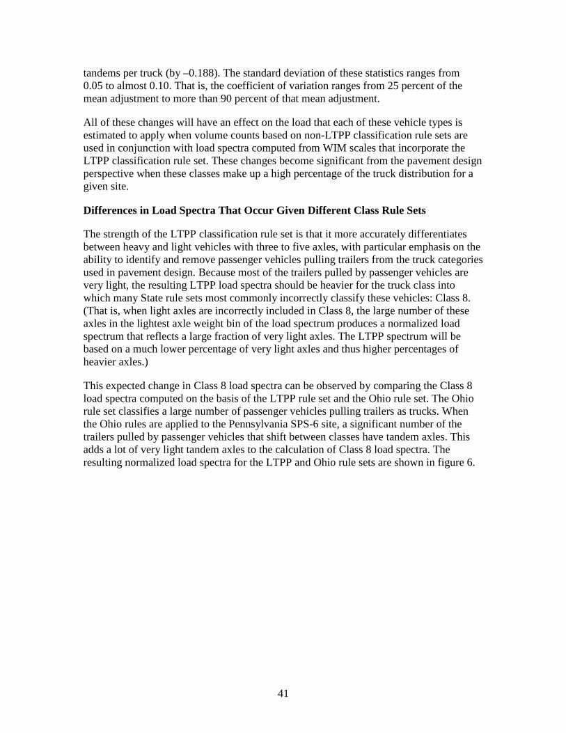
tandems per truck (by –0.188). The standard deviation of these statistics ranges from 0.05 to almost 0.10. That is, the coefficient of variation ranges from 25 percent of the mean adjustment to more than 90 percent of that mean adjustment.

All of these changes will have an effect on the load that each of these vehicle types is estimated to apply when volume counts based on non-LTPP classification rule sets are used in conjunction with load spectra computed from WIM scales that incorporate the LTPP classification rule set. These changes become significant from the pavement design perspective when these classes make up a high percentage of the truck distribution for a given site.

Differences in Load Spectra That Occur Given Different Class Rule Sets

The strength of the LTPP classification rule set is that it more accurately differentiates between heavy and light vehicles with three to five axles, with particular emphasis on the ability to identify and remove passenger vehicles pulling trailers from the truck categories used in pavement design. Because most of the trailers pulled by passenger vehicles are very light, the resulting LTPP load spectra should be heavier for the truck class into which many State rule sets most commonly incorrectly classify these vehicles: Class 8. (That is, when light axles are incorrectly included in Class 8, the large number of these axles in the lightest axle weight bin of the load spectrum produces a normalized load spectrum that reflects a large fraction of very light axles. The LTPP spectrum will be based on a much lower percentage of very light axles and thus higher percentages of heavier axles.)

This expected change in Class 8 load spectra can be observed by comparing the Class 8 load spectra computed on the basis of the LTPP rule set and the Ohio rule set. The Ohio rule set classifies a large number of passenger vehicles pulling trailers as trucks. When the Ohio rules are applied to the Pennsylvania SPS-6 site, a significant number of the trailers pulled by passenger vehicles that shift between classes have tandem axles. This adds a lot of very light tandem axles to the calculation of Class 8 load spectra. The resulting normalized load spectra for the LTPP and Ohio rule sets are shown in figure 6.

41

Figure 6. Graph. Comparison of Class 8 normalized tandem load spectra

for the LTPP and Ohio rule sets.

The Class 8 load spectra for these two rule sets are based on essentially the same number of heavy axles. However, the spectra for the Ohio rule set contain a very large number of light axles that are not included in the LTPP spectra, so the total number of axles in the Ohio rule set load spectra is larger. Because of these extra axles, the denominator used to convert the actual load spectrum into the normalized version shown in figure 6 is larger for the Ohio rule set, and therefore the fraction of axles attributed to each of the heavier load ranges is smaller for the Ohio spectrum than for the LTPP spectrum. In contrast, the normalized load spectrum for the Ohio rule set has a considerably greater proportion of axles in the two lightest load ranges. Thus, the normalized Ohio spectrum is much lighter than the normalized LTPP spectrum.

If the light Ohio load spectra were multiplied by the much greater Class 8 vehicle volume produced by the Ohio rules, the total number of heavy axles would be the same as that computed with the LTPP rule set’s load spectra and the LTPP rule set’s Class 8 volume estimate.8 However, if the larger Ohio Class 8 volume were multiplied by the heavier LTPP load spectra, the total load (cumulative over all load ranges) computed for this class of trucks would be much higher than that applied by actual truck traffic.

While the Class 8 example above is a good illustration of how the load spectrum for a specific vehicle class and axle type can change—given a different classification rule set—changes do not occur in just this one vehicle class or axle type. Changes occur simultaneously across multiple vehicle classes and differ depending on the vehicle classification rule set to which the LTPP rule set is compared. The combinations of these

8 The Ohio rule set would also estimate that a very large number of very light axles would “load” this pavement section. These axles are not present in the LTPP load estimate because the LTPP rule set places these vehicles in Classes 2 and 3, which are not incorporated into the load estimation process.

0

0.02

0.04

0.06

0.08

0.1

0.12

0.14

0.16

0.18

6000 10000 14000 18000 22000 26000 30000 34000 38000 42000 46000

Frac

tion

of A

xles

in W

eigh

t Ran

ge

Maximum Load in Weight Range (lb)

LTPP

Ohio

42

multiple changes are extremely difficult to predict, in large part because at each site, the vehicles transferring into or out of a given classification may be light or heavy (particularly in the heavier vehicle classes), and until a site has been examined carefully, analysts cannot know whether the group of vehicles changing classes makes up a large or small percentage of the vehicles in each class.

The variety of effects generated by using different State classification rule sets is illustrated in figure 7 and figure 8. Figure 7 shows the normalized single-axle load spectra for Class 8 vehicles for the Pennsylvania SPS-6 site under nine different classification rule sets. Figure 8 shows the normalized Class 8 tandem spectra for those same rule sets.

These two figures readily show which classification rule sets significantly change the nature of the vehicles (and thus the loading characteristics of the vehicles) identified as Class 8. The Florida AVC, Ohio, Wisconsin, and Washington systems all primarily rely on axle spacing to differentiate these vehicles, whereas the California WIM, LTPP, and Florida WIM rule sets all use weight to help with this differentiation. The rule sets produce very different outcomes. One interesting observation is that the California AVC system matches the California WIM system reasonably well, despite its inability to use weight data in that differentiation.

Figure 7. Graph. Normalized single-axle load spectra for Class 8 vehicles,

Pennsylvania SPS-6 site, given different classification rule sets.

0

0.05

0.1

0.15

0.2

0.25

Frac

tion

of A

xles

in E

ach

Load

Ran

ge

Upper Bound of Load Range (pounds)

LTPP

WA WIM

Wis

Missouri

FLA WIM

FLA AVC

CA WIM

CA AVC

Ohio

43

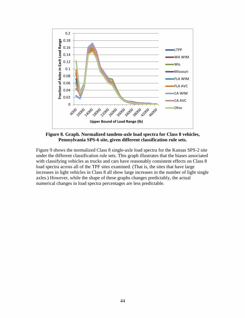
Figure 8. Graph. Normalized tandem-axle load spectra for Class 8 vehicles,

Pennsylvania SPS-6 site, given different classification rule sets.

Figure 9 shows the normalized Class 8 single-axle load spectra for the Kansas SPS-2 site under the different classification rule sets. This graph illustrates that the biases associated with classifying vehicles as trucks and cars have reasonably consistent effects on Class 8 load spectra across all of the TPF sites examined. (That is, the sites that have large increases in light vehicles in Class 8 all show large increases in the number of light single axles.) However, while the shape of these graphs changes predictably, the actual numerical changes in load spectra percentages are less predictable.

0

0.02

0.04

0.06

0.08

0.1

0.12

0.14

0.16

0.18

0.2

Frac

tion

of A

xles

in E

ach

Load

Ran

ge

Upper Bound of Load Range (lb)

LTPP

WA WIM

Wis

Missouri

FLA WIM

FLA AVC

CA WIM

CA AVC

Ohio

44

Figure 9. Graph. Normalized single-axle load spectra for Class 8 vehicles,

Kansas SPS-2 site, given different classification rule sets.

These figures also show that the effect of adding cars pulling trailers to Class 8 has a much more significant impact on the visual shape of the normalized single-axle load spectra than it does on that of the tandem axle spectra. This is likely because cars pulling trailers add at least two single axles per vehicle (and sometimes three or four single axles) to the load spectra for Class 8 when they are incorrectly shifted into this vehicle class. On the other hand, only a fraction of these vehicles have trailers with tandem axles, and they only have one tandem axle per vehicle. Therefore, the shift toward light axles may not be as strong in the tandem axle category when a State rule set places pickups pulling trailers in Class 8.

The patterns shown above follow a consistent bias: specific types of cars with trailers either are—or are not—included in Class 8. Those classification systems that include more passenger vehicles in Class 8 produce load spectra that have large numbers of light single and tandem axles. Those rule sets that are more restrictive have heavier load spectra.

In the larger truck categories, there is generally less consistency. Although the same bias concept does exist, in the case of larger trucks, there are two other important factors: 1) are the specific vehicle configurations identified by those biases present, and 2) are those vehicles light or heavy at a particular site?

0.00

0.05

0.10

0.15

0.20

0.25

3000

4000

5000

6000

7000

8000

9000

1000

011

000

1200

013

000

1400

015

000

1600

017

000

1800

019

000

2000

0

Frac

tion

of A

xles

in E

ach

Load

Ran

ge

Uppper Bound of Load Range

LTPP

WA WIM

Wis

Missouri

FLA WIM

FLA AVC

CA WIM

CA AVC

Ohio

45

In the Class 8 example, there is a reasonably large number of passenger vehicles pulling trailers, and all of those vehicles tend to be light. Therefore, the same basic trend occurs at all sites. The only question is how large those changes are at a given site. For heavier truck classes, neither of these factors is constant.

Once again the Class 13 and Class 10 examples illustrate the impact of those biases. The load spectra change in the same varied way that the estimated number of axles per truck changes for these classes, and for the same basic reasons.

Figure 10 shows how the heaviest portion of the normalized load spectra for quad axles changes for Class 10 under the different classification rule sets at the Maryland SPS-5 site. Figure 11 shows this same portion of the quad-axle load spectra for Class 13 at the Tennessee SPS-6 site. Figure 12 and figure 13 show these same two graphs, but for the New Mexico SPS-5 site. Because the vehicles are very different, and even more important, because the loads carried by those vehicles are very different, the effects of the classification shift differ.

Figure 10. Graph. Normalized quad-axle load spectra for Class 10 vehicles,

Maryland SPS-5 site, given different classification rule sets.

In figure 10, extreme peaks result at 54,000 lb for the LTPP and California WIM load spectra. These peaks occur because only one quad axle is observed in Class 10 under the LTPP and California WIM classification rule sets. That one axle falls in the 54,000-lb load range bin. Thus, this load spectrum has 100 percent of all quad axles in this load range. Just as important, no Class 10 quad axles are observed at this site when using the California AVC rule set. Conversely, the Washington, Ohio, and to a lesser extent, Wisconsin rule sets all observe a significant, heavy set of quad axles heavier than

0.00

0.20

0.40

0.60

0.80

1.00

Frac

tion

of A

xles

In E

ach

Loa

d R

ange

Upper Bound of Each Load Range (pounds)

LTPPWA WIMWisMissouriFLA WIMFLA AVCCA WIMOhio

46

72,000 lb, while the two Florida rule sets observe a large percentage of quad axles in the 60,00-lb range.

When a classification rule set introduces large numbers of quad axles into this classification, the spike shown in the LTPP classification disappears. The specific axle that caused the LTPP rule set spike is still present in the load spectrum calculation, but it is now only one of many. Therefore, in this case, this particular load spectrum becomes heavier simply because a different classification rule set was applied. However, if that one axle had been very heavy, the alternative rule set could just as easily have made those load spectra lighter.

Figure 11 continues this example by now examining the quad distribution of Class 13 at the same Maryland site. In figure 11, we can see that the heavy quad axles observed in Class 10 in the Washington, Ohio, and Wisconsin rule sets in figure 10 now appear in Class 13 when the Florida and California classification rule sets are used. They are missing from both figures in the LTPP rule set, because these axles were part of trucks that were left unclassified by the LTPP rules. Also note that the large number of 60,000-lb axles observed in figure 10 (Class 10) for the Florida sites are not present in Class 13 for any of the classification rule sets. These axles were not exchanged between Class 10 and 13. Instead, these axles belong to trucks that are classified as Class 7 by the Washington, Ohio, and Wisconsin rule sets, and thus are not included in either figure 10 or figure 11. The lack of heavy axles in Class 13 for the Washington, Wisconsin, and Ohio rule sets means that for those rule sets, the Class 13 quad load spectrum is quite light for this Maryland site, while it is quite heavy for the California and Florida rule sets.

Class 13 quads are not always made lighter by the use of rule sets like Washington’s. Figure 12 shows that at the Tennessee SPS 6 site, the addition of the multi-axle Class 13 vehicles, which are not classified by the LTPP rules, creates a much heavier quad load spectrum than is observed in the LTPP spectrum, despite the fact that many of the LTPP Class 13 vehicles are reclassified as Class 10s by the Washington rules. Similarly, at this site, the Florida WIM rules have produced a much heavier load spectrum than most of the other rule sets. At this site, the Florida WIM rule set has observed trucks with more than 300 more quad axles than the Florida AVC rule set, and those additional axles generate a much heavier load spectrum. Conversely, the Ohio rule set classifies three-quarters of the trucks that LTPP designates as Class 13 as Class 10 trucks. Many of the heavy axles moved to Class 10 along with those trucks, and the resulting quad load spectrum is therefore much lighter than reported using the LTPP rules.

47

Figure 11. Graph. Normalized quad-axle load spectra for Class 13 vehicles, Maryland SPS-5 site, given different classification rule sets.

Figure 12. Graph. Normalized quad-axle load spectra for Class 13 vehicles,

Tennessee SPS-6 site, given different classification rule sets.

0.00

0.10

0.20

0.30

Frac

tion

of A

xles

In

Eac

h L

oad

Ran

ge

Upper Bound of Each Load Range (pounds)

LTPPWA WIMWisMissouriFLA WIMFLA AVCCA WIMCA AVCOhio

0

0.02

0.04

0.06

0.08

0.1

0.12

0.14

0.16

0.18

1200

018

000

2400

030

000

3600

042

000

4800

054

000

6000

066

000

7200

078

000

8400

090

000

9600

0

Frac

tion

of A

xles

in E

ach

Load

Ran

ge

Upper Bound of Load Range (lb)

LTPP

WA WIM

Wis

Missouri

FLA WIM

FLA AVC

CA WIM

CA AVC

Ohio

48

These same changes are not present at the New Mexico SPS-5 site, even though the classification rule sets shift the same types of vehicles. Because the number of vehicles of each type and the weights they carry are different, the impacts of the rule set are different.

In figure 13, unlike figure 12, there are very few loaded axles. In fact, the LTPP rule set counts very few axles at all. Therefore, the differences in load spectra are essentially the normalized load spectra of the vehicles shifting into Class 10. In the Florida AVC rule set, only 10 quad axles are included in Class 10. Two of them are moderately heavy, explaining the peak loading observed. None of the other rule sets shift vehicles with heavy quad axles into Class 10, even though several rule sets (such as Washington’s) result in counting more than 100 quad axles on Class 10 trucks.

Figure 13. Graph. Normalized quad axle load spectra for class 10 vehicles,

New Mexico SPS-5 site, given different classification rule sets.

In figure 14, the major differences among heavy axle loads come from the vehicles that are not classified by the LTPP rules. In the Washington and Florida WIM rule sets, many of these vehicles are identified as Class 13, and the heavy axles of these vehicles are incorporated into this normalized load spectrum. In the classification rule sets that do not identify these vehicles as Class 13, these heavy quad axles remain in Class 15 and therefore do not appear in this graph. They also are not included in the LTPP load estimate, regardless of the classification rule set used to estimate the truck volumes used in the pavement design.

0

0.1

0.2

0.3

0.4

0.5

0.6

0.7

1200

018

000

2400

030

000

3600

042

000

4800

054

000

6000

066

000

7200

078

000

8400

090

000

Frat

ion

of A

xles

in E

ach

Load

Ran

ge

Upper Bound of Load Range (lbs)

LTPP

WA WIM

Wis

Missouri

FLA WIM

FLA AVC

CA WIM

CA AVC

Ohio

49

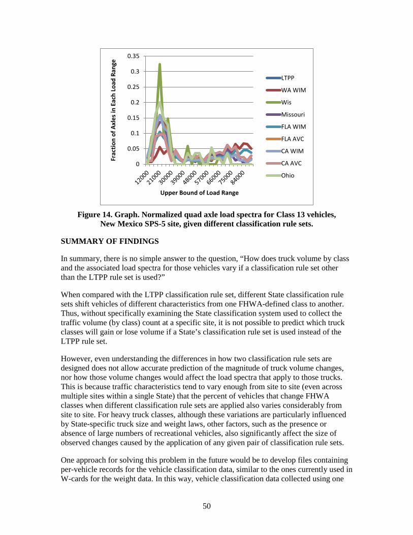
Figure 14. Graph. Normalized quad axle load spectra for Class 13 vehicles,

New Mexico SPS-5 site, given different classification rule sets.

SUMMARY OF FINDINGS

In summary, there is no simple answer to the question, “How does truck volume by class and the associated load spectra for those vehicles vary if a classification rule set other than the LTPP rule set is used?”

When compared with the LTPP classification rule set, different State classification rule sets shift vehicles of different characteristics from one FHWA-defined class to another. Thus, without specifically examining the State classification system used to collect the traffic volume (by class) count at a specific site, it is not possible to predict which truck classes will gain or lose volume if a State’s classification rule set is used instead of the LTPP rule set.

However, even understanding the differences in how two classification rule sets are designed does not allow accurate prediction of the magnitude of truck volume changes, nor how those volume changes would affect the load spectra that apply to those trucks. This is because traffic characteristics tend to vary enough from site to site (even across multiple sites within a single State) that the percent of vehicles that change FHWA classes when different classification rule sets are applied also varies considerably from site to site. For heavy truck classes, although these variations are particularly influenced by State-specific truck size and weight laws, other factors, such as the presence or absence of large numbers of recreational vehicles, also significantly affect the size of observed changes caused by the application of any given pair of classification rule sets.

One approach for solving this problem in the future would be to develop files containing per-vehicle records for the vehicle classification data, similar to the ones currently used in W-cards for the weight data. In this way, vehicle classification data collected using one

0

0.05

0.1

0.15

0.2

0.25

0.3

0.35

Frac

tion

of A

xles

in E

ach

Load

Ran

ge

Upper Bound of Load Range

LTPP

WA WIM

Wis

Missouri

FLA WIM

FLA AVC

CA WIM

CA AVC

Ohio

50

algorithm or rule set could be reprocessed if a different algorithm or rule set is desired (for example, to align vehicle classification and weight data collected using two different classification rule sets).

The wide variety of changes observed in truck volumes given the application of any specific State classification rule set are further reflected in the axle weight spectra produced from those truck volumes.

When these differences in load spectra are combined with the volume changes observed in individual truck classes, it appears that significant differences in predicted pavement loading for many vehicle classes may occur. The size of these differences is explored in the next chapter of this report. Whether these differences are sufficient to affect pavement design outcomes is discussed in Part II of this report.

51

CHAPTER 4. EVALUATION OF LIKELY ERRORS IN THE TOTAL TRAFFIC LOADING ESTIMATE WHEN USING LOAD SPECTRA COMPUTED WITH

THE LTPP CLASS RULE SET AND TRUCK VOLUMES FROM STATE-SPECIFIC RULE SETS

ANALYSIS PURPOSE

The previous chapter described the kinds of changes (errors) that occur in the outcome of the vehicle classification process when different classification rule sets are applied to the basic axle weight and spacing data collected by WIM and AVC equipment, and the effect those changes have on the computation of normalized load spectra. When truck volumes are counted using one classification rule set and load spectra are computed using a different classification rule set, mismatches between the volumes reported and load spectra used create errors in the traffic load estimate used for pavement design. Whether those errors over- or under-estimate the load varies depending on which classification rule sets are used and what the vehicle characteristics are at each site.

This chapter explores the combined effects of all of the previously examined changes in classification. It computes traffic loads using truck volume data computed from the individual truck classification records at LTPP SPS TPF sites as processed using a variety of different classification rule sets and applied against the LTPP load spectra. These results are compared against the known traffic load at the SPS TPF sites. The errors computed are used to estimate the size and nature of traffic load errors that can be expected if load spectra from the SPS TPF sites are used at LTPP test sections that do not have valid, site-specific load spectra, and that use truck volume counts based on classification counts made using State-specific vehicle classification rule sets.

METHODOLOGY FOR TESTING THE APPLICABILITY OF LTPP WIM RULE SET

To understand the relative importance to pavement design of the wide variety of biases/ changes in estimated traffic volume that are caused by the use of alternative vehicle classification rule sets, it is necessary to simplify the traffic load estimate. This is most commonly done by selecting a set of coefficients or factors that allow conversion of a set of axles of different weights into a new, single value. These coefficients serve as weights of relative importance of individual axle weight measurements with respect to their effect on pavement deterioration.

In this approach, axle loads are divided into load spectra. Each weight bin within a load spectrum is assigned a weight (or impact factor) that is related to the damaging potential caused by a single application of an axle of that weight. The impact factors provide a measure of the relative importance of one load level against another with regard to potential pavement damage. (Note that these impact factors are not intended to be used in

53

a direct computation of pavement damage because different pavement deterioration mechanisms are expected to have different sensitivity to various load levels.)9

Once a conversion method has been selected, it is possible to make direct comparisons of the combined effects of using different vehicle classification rule sets for the development of load spectra, and the determination of traffic volumes by vehicle classification that are used in the pavement design process.

The axle load spectra used in this study come from the LTPP SPS TPF data. They are computed as normalized load spectra for each type of axle (single, tandem, tridem, and quad) for each class of vehicle. To develop an estimate of the total annual loading for the analysis, the following procedure was applied:

1. The weight factor for each weight bin (load range) shown in table 12 was multiplied by the percentage of axles in the same weight bin of the axle load spectrum and the products summed across all weight bins. This was done separately using axle load spectra for each vehicle class and axle type.

2. The result from step 1 was multiplied by the total number of axles occurring for the year being examined obtained for the vehicle classification rules being examined. This was done separately for each vehicle class and axle type.

3. The results from step 2 were summed across all vehicle classes and axle types to produce an estimate of converted total annual impact load.

Using this procedure, the estimates of total annual impact load for one classification rule set can be compared with that produced by another classification rule set.

A single total annual impact load value was then computed for each of the 18 TPF sites for which load spectra and vehicle classification data were available for this analysis. At most sites, data for a complete year were used to compute this single loading estimate. (In a few cases, the site had slightly less than 12 months of traffic data, but the available data were more than sufficient to estimate the effects of using different classification rule sets. These sites are treated as though there were 12 months of data present.)

9 The specific method chosen to compute any given set of impact factors will affect the results of such a study. Only one set of impact factors is presented in this report. The choice of a different set of impact factors based on different damage criteria will produce slightly different numerical results than those presented in this report. The project team is confident that the choice of any commonly agreed upon set of impact factors in place of the one chosen will not significantly alter the basic conclusions of this report.

54

Table 12. Impact factors used to compute total loading estimate. Single Tandem Tridem Quad

Weight Bin (lb) Factor Weight Bin (lb) Factor Weight Bin (lb) Factor Weight Bin (lb) Factor 0–999 0 0–1,999 0 0–2,999 0 0–2,999 0 1,000–1,999 0 2,000–3,999 0 3,000–5,999 0 3,000–5,999 0 2,000–2,999 0 4,000–5,999 0 6,000–8,999 0 6,000–8,999 0 3,000–3,999 0 6,000–7,999 0 9,000–11,999 0 9,000–11,999 0 4,000–4,999 0 8,000–9,999 0 12,000–14,999 0 12,000–14,999 0 5,000–5,999 0 10,000–11,999 0 15,000–17,999 0.04 15,000–17,999 0 6,000–6,999 0 12,000–13,999 0.01 18,000–20,999 0.09 18,000–20,999 0.02 7,000–7,999 0 14,000–15,999 0.04 21,000–23,999 0.15 21,000–23,999 0.05 8,000–8,999 0.02 16,000–17,999 0.08 24,000–26,999 0.21 24,000–26,999 0.09 9,000–9,999 0.04 18,000–19,999 0.14 27,000–29,999 0.28 27,000–29,999 0.14 10,000–10,999 0.08 20,000–21,999 0.22 30,000–32,999 0.35 30,000–32,999 0.2 11,000–11,999 0.12 22,000–23,999 0.3 33,000–35,999 0.43 33,000–35,999 0.27 12,000–12,999 0.18 24,000–25,999 0.4 36,000–38,999 0.53 36,000–38,999 0.34 13,000–13,999 0.24 26,000–27,999 0.51 39,000–41,999 0.64 39,000–41,999 0.42 14,000–14,999 0.31 28,000–29,999 0.62 42,000–44,999 0.76 42,000–44,999 0.52 15,000–15,999 0.4 30,000–31,999 0.75 45,000–47,999 0.92 45,000–47,999 0.62 16,000–16,999 0.49 32,000–33,999 0.89 48,000–50,999 1.1 48,000–50,999 0.73 17,000–17,999 0.59 34,000–35,999 1.04 51,000–53,999 1.32 51,000–53,999 0.85 18,000–18,999 0.71 36,000–37,999 1.21 54,000–56,999 1.58 54,000–56,999 0.99 19,000–19,999 0.85 38,000–39,999 1.4 57,000–59,999 1.9 57,000–59,999 1.14 20,000–20,999 1.01 40,000–41,999 1.63 60,000–62,999 2.27 60,000–62,999 1.3 21,000–21,999 1.19 42,000–43,999 1.9 63,000–65,999 2.71 63,000–65,999 1.47 22,000–22,999 1.41 44,000–45,999 2.23 66,000–68,999 3.22 66,000–68,999 1.66 23,000–23,999 1.67 46,000–47,999 2.63 69,000–71,999 3.82 69,000–71,999 1.87 24,000–24,999 1.99 48,000–49,999 3.13 72,000–74,999 4.51 72,000–74,999 2.1 25,000–25,999 2.38 50,000–51,999 3.74 75,000–77,999 5.3 75,000–77,999 2.35 26,000–26,999 2.85 52,000–53,999 4.49 78,000–80,999 6.2 78,000–80,999 2.63 27,000–27,999 3.43 54,000–55,999 5.42 81,000–83,999 7.22 81,000–83,999 2.93 28,000–28,999 4.12 56,000–57,999 6.56 84,000–86,999 8.37 84,000–86,999 3.26 29,000–29,999 4.96 58,000–59,999 7.95 87,000–89,999 9.66 87,000–89,999 3.62 30,000–30,999 5.97 60,000–61,999 9.64 90,000–92,999 11.09 90,000–92,999 4.02 31,000–31,999 7.18 62,000–63,999 11.67 93,000–95,999 12.68 93,000–95,999 4.46 32,000–32,999 8.62 64,000–65,999 14.11 96,000–98,999 14.44 96,000–98,999 4.94 33,000–33,999 10.33 66,000–67,999 17 99,000–101,999 16.37 99,000–101,999 5.47 34,000–34,999 12.35 68,000–69,999 20.43 102,000–104,999 18.48 102,000–104,999 6.06 35,000–35,999 14.72 70,000–71,999 24.47 105,000–107,999 20.78 105,000–107,999 6.71 36,000–36,999 17.48 72,000–73,999 29.19 108,000–110,999 23.28 108,000–110,999 7.42 37,000–37,999 20.7 74,000–75,999 34.68 111,000–113,999 25.98 111,000–113,999 8.2 38,000–38,999 24.41 76,000–77,999 41.04 114,000–116,999 28.9 114,000–116,999 9.06 ≥ 39,000 28.7 ≥ 78,000 48.37 ≥ 117,000 32.03 ≥ 117,000 10.01 Load spectra and vehicle volumes by classification were computed for each of the available TPF sites, using each of the different classification rule sets tested. A single statistic representing total annual impact traffic load estimate was then computed for each TPF site for the following:

• LTPP load spectra and traffic volumes by classification computed using the LTPP spectra.

• LTPP load spectra and traffic volumes using each of the State classification rule sets.

55

These outputs were then compared. The value computed using the LTPP load spectra and LTPP volumes is considered “ground truth” for this analysis.

The difference in the total annul traffic impact loading estimates that result from using different classification rule sets for count versus weight data collection is expressed as the ratio of the computed traffic load divided by the LTPP ground truth value (i.e., [Total Annual Impact Load with LTPP Load Spectra and State-Specific Class Volumes] divided by [Total Annual Impact Load with LTPP Load Spectra and LTPP Class Volumes]).

This statistic is referred to as the “Class Ratio” in this report, and this term is used throughout the remainder of this report to describe the results of the analysis of the effects of using traffic volumes collected with State-specific classification rule sets.

A Class Ratio greater than 1 indicates an increase in estimated traffic load when compared with what the LTPP system alone would have computed at these TPF sites. A ratio less than 1 indicates a decrease in estimated traffic load. At each TPF site, a mean and standard deviation of the Class Ratio values was computed across all of the tested classification rule sets. The mean and standard deviation are taken as the reasonable range of the “errors” associated with using different classification rule sets for developing load spectra and traffic volume by classification estimates.

ANALYSIS OF EXPECTED ERRORS IN TOTAL TRAFFIC LOADING

As noted earlier in this report, the use of different classification rule sets changes how some vehicles are classified. When a different classification rule set is used for load spectra development than is used to develop the count of traffic volume by vehicle classification, the computed number of heavy and light axles is altered from the correct value. Whether this change increases or decreases the total load estimate depends on which classification rule set is used for load spectra development and which is used for vehicle volume estimation. It also depends on what the vehicle characteristics are at any given site. In some cases, whether a given classification rule set increases or decreases the total traffic load is primarily a function of the site-specific traffic stream.

For this analysis, the primary objective was to determine the size of errors imposed on traffic load estimates when using load spectra developed using the LTPP classification rule set, but applied at sites where the traffic volume by classification estimate comes from a State-specific classification rule set.

Of the seven State classification rule sets tested in this specific analysis, two (Washington WIM and Florida AVC) produced a Class Ratio that was greater than 1 at all 18 test sites. (That is, they consistently produced a larger traffic load than the LTPP rule set alone would have estimated.) Two additional rule sets (Wisconsin and Missouri) produced Class Ratios greater than 1 at a majority of sites (15 increase/3 decrease and 10 increase/ 8 decrease, respectively.) One classification rule set (California AVC) produced Class Ratios that were less than 1 at all TPF sites, and two rule sets produced Class Ratios less than one at a large majority of sites (2/16 for the Florida WIM and 5/13 for the California WIM rule set).

56

Table 13 shows the mean and standard deviation of the Class Ratio along with the number of increased and decreased traffic load estimates for each the 18 TPF sites tested for each of the examined State classification rule sets.

If changes are examined at the site level rather than by classification rule set, another trend emerges. At sites where heavy traffic loads occur, very little change in the load estimate occurs when different classification rule sets are used, regardless of which different rule set is used. However, if annual traffic loads are light, the potential for large percentage changes in traffic loading estimates caused by the use of different classification rule sets increases greatly. This can be seen in figure 15.

Table 13. Effect of using State rule set volumes and LTPP load spectra averaged across 18 TPF sites.

State Rule Set Mean Class

Ratio

Standard Deviation of Class Ratio

Number of Sites With Increased

Load Estimates

Number of Sites With Decreased

Load Estimates

Washington WIM 1.07 0.08 18 0 Wisconsin 1.05 0.06 15 3 Missouri 1.00 0.01 10 8 Florida WIM 0.98 0.03 2 16 Florida AVC 1.06 0.07 18 0 California WIM 0.98 0.05 5 13 California AVC 0.95 0.04 0 18

WIM = Weight in Motion AVC = Automatic Vehicle Classification

57

Note: The equation in the figure describes the best fit line obtained from a linear regression for the data shown. The goodness of fit is given by the R2 value.

Figure 15. Graph. Plot of total annual impact load and standard deviation of class ratio.

Further examination of the TPF data shows that the loading computations for sites with very large traffic loads tend to be dominated by high volumes of large, heavy trucks. In the vast majority of cases, the most significant contributors to that load are Class 9 trucks. This can be seen in figure 16, which illustrates the relationship between total load and the percentage of trucks in Class 9 at the 18 TPF test sites.

y = -0.2x + 0.1795R² = 0.76178

0

0.02

0.04

0.06

0.08

0.1

0.12

0.14

0.16

0.18

0% 10% 20% 30% 40% 50% 60% 70% 80% 90% 100%

Stan

dard

Dev

iatio

n of

Cla

ss R

atio

Percent of Trucks in Classes 9 Through 13

58

Figure 16. Graph. Total annual impact load versus percent of trucks in Class 9.

Because Class 9 trucks rarely change classification when alternative classification rule sets are used, sites at which Class 9 dominate the traffic loading do not show much variation in total traffic load when different classification rule sets are applied.

On the other hand, at those sites where a significant portion of load is contributed by smaller trucks (Classes 8 and below), the use of alternative classification rule sets can have a much larger impact. This correlation between high percentages of smaller trucks (also stated as a low percentage of Class 9 trucks) and a high standard deviation of the Class Ratio can be seen in figure 17.

Tot

al A

nnua

l Im

pact

Loa

d

59

Note: The equation in the figure describes the best fit line obtained from a linear regression for the data shown. The goodness of fit is given by the R2 value.

Figure 17. Graph. Standard deviation of class ratio versus percent of trucks in Class 9.

However, figure 17 also shows that Class 9 percentage is not the only factor that influences the size of the error that can be caused by using different classification rule sets for the load spectra and volume by classification inputs. The outlier data point in figure 17 is the Louisiana TPF site. This site has a very high percentage of unloaded Class 9 trucks and an unusually large number of very heavy trucks in Classes 10 and 13. When compared with the LTPP rule set, the Class 10 and 13 trucks change classification under many State rule sets. The combined effect of light Class 9 loads and heavy Class 10 and 13 loads yields a higher than expected change in total traffic load when the effects of different classification rule sets are compared.

CONCLUSIONS AND RECOMMENDATIONS

The analysis presented above shows that when a stream of traffic data is processed using different vehicle classification rule sets, the truck volume counts and load spectra computed by those two different rule sets can be significantly different in at least some vehicle classes, including Classes 4–8, 10, and 13. As a result, the total traffic load computed using vehicle classification estimates from one device and a load spectra computed from data collected from a second device that uses a different classification rule set, including the LTPP rule set, has the potential to contain some errors. The size and significance of that error is highly variable, changing considerably from one

y = -0.225x + 0.1822R² = 0.77492

0

0.02

0.04

0.06

0.08

0.1

0.12

0.14

0.16

0.18

0% 10% 20% 30% 40% 50% 60% 70% 80% 90%

Stan

dard

Dev

iatio

n of

Cla

ss R

atio

Percent of Trucks in Class 9

Louisiana Site

60

classification rule set to another and even from one site to another. Sites that have a high percentage of Class 9 vehicles are not likely to be significantly affected by these errors.

It is also clear from the analysis that the effect of using the LTPP load spectra and State-specific classification count data on the accuracy of the total traffic load estimate is nearly impossible to predict without actually performing a detailed analysis for each site and each State classification system. Variability in the errors comes from the following two sources:

• Specific differences in the parameters used to classify vehicles that are found in the various State and LTPP classification rule sets.

• Actual percentage of vehicles present at any given pavement design site that fit within the set of vehicles that change classifications when the LTPP rule set is applied in place of the State rule set.

To simply illustrate these factors, assume that the State rule set classifies all cars pulling trailers as trucks, and the LTPP rule set classifies no cars pulling trailers as trucks. The “different parameters” are the ability to identify a car. If a road is restricted to heavy trucks and actually experiences no cars pulling trailers, then this difference in design has no effect on the truck volume estimate. On the other hand, if the road experiences very heavy recreational vehicle traffic, there will be many such vehicles, and the State rule set will badly overestimate the volume of trucks. This overestimation of truck volume when multiplied by the LTPP load spectra will overestimate the traffic load created by that class of vehicles.

Whether this overestimation of load is significant is a function of what other traffic loads are being applied to that pavement. That is, if the only trucks using the road are those that can be “confused” with cars pulling trailers, the total load estimate will be very poor. On the other hand, if the road carries a large number of trucks in other categories that are not affected by the choice of classification system (such as classic five-axle tractor semi-trailers), then the overall load estimate is likely to be reasonably accurate, despite the errors caused by using two different classification rule sets.

Application of the LTPP Load Spectra Collected Using the LTPP WIM Rule Set at Other Pavement Analysis Sites

The implications of these findings for the application of load spectra developed using the LTPP classification rules are fairly straightforward. It should be possible to use LTPP load spectra at other LTPP test sites without the risk of introducing significant error in the traffic load calculation whenever one of the following conditions occurs:

• High traffic loadings (e.g., total annual impact loading estimate is more than 300,000) are present.

61

• Greater than 60 percent of trucks in Classes 4 to 13 are in Class 9.10

Sites with annual traffic loading above 300,000 should experience less than 4-percent additional error (with a 95-percent level of confidence) in their total annual impact loading estimates as a result of the use of two vehicle classification rule sets (the LTPP rule set plus a State rule set) in the development of their load estimate. Even with total annual impact loading estimates below 300,000, the added error caused by the mismatch in vehicle classifications from the use of different AVC and WIM rule sets should be below 12 percent (with 95-percent confidence), if Class 9 trucks represent more than 60 percent of all truck volume (i.e., 60 percent of volume in Classes 4 through 13).

At LTPP test sites that fall outside the above parameters (i.e., have lower total annual impact loading estimates and less significant Class 9 truck volume percentages), the use of the LTPP TPF load spectra can result in more significant errors in the estimated traffic load. The data available for tests in this project suggest that at these sites, the 95th percentile error bounds in annual pavement loading estimate (resulting from use of different classification rule sets) ranges between 10 and 34 percent.11 In general, the greater the percentage of total traffic load owing to truck Classes 5 and 8, the greater the error will be when using load spectra created with the LTPP rule set.

Based strictly on the computation of the annual traffic loading estimate, it is therefore not recommended to use load spectra from the LTPP TPF sites collected using the LTPP classification rule set in conjunction with pavement study sites that have at least one of the following:

• Total annual impact loading estimates below 50,000 (unless a very high percentage of those loads come from Class 9 trucks).

• Less than 50 percent of truck volume in Class 9 among Classes 4 through 13.

This recommendation applies unless additional work is performed that shows that the specific State classification rule set used to collect truck volume data does not create significantly different truck volumes in truck Classes 5 and 8 than the LTPP rule set when applied to the same traffic stream.

Additional research done to test the sensitivity of the pavement analysis models to traffic load provides further insight into when the outcome of the pavement analysis is affected

10These percentage error estimates are computed as two times the standard deviation of the Class Ratio observed in tests performed for this project (see figure 15 through figure 17), assuming normal distribution of errors. 11A much larger source of error is likely to be the error associated with selecting load spectra from different site(s) and applying them to a site that may have different loading characteristics. This is the subject of a different LTPP analysis task. These errors are caused when non-site-specific load spectra are used, causing the differences in the percent of loaded trucks (or the percent of illegally loaded axles) between the actual site and what is present in the non-site-specific load spectra. This is likely to create far larger errors in the traffic load estimate than would be caused by the use of mismatched vehicle classification rule sets.

62

by changes in traffic loading. The following section discusses the development of the traffic loading scenarios used to perform those tests. The results of those pavement model sensitivity tests are provided in the final recommendations presented in Chapter 7 and include recommendations about when and where the LTPP SPS TPF load spectra can be used when site-specific load spectra are not available.

Recommended Scenarios for Sensitivity Tests of Pavement Design Models

Because it is practically impossible to test the sensitivity of the MEPDG to all possible combinations of site-specific vehicle streams and vehicle classification rule sets, a decision was made to identify and test a set of the worst cases that are likely to result in the maximum differences in traffic load observed when using one consistent classification rule set versus using a load spectra based on the LTPP WIM rule set and truck volume data collected using a State-specific vehicle classification rule set. The logic behind this approach is that if pavement design outcomes are not sensitive to these extreme differences, then all other less extreme differences can be considered insignificant. On the other hand, if significant differences are observed, more detailed site-specific analyses may be required.

To test the sensitivity of the pavement design models to differences in loading estimates resulting from application of different classification rules, five alternative traffic loading inputs were identified. The recommended loads are drawn directly from TPF sites. They include two load estimates under very heavy loading conditions and three load estimates under fairly light loading conditions.

The five input scenarios are intended to examine how significantly different the predicted pavement design and analysis outcomes are when different traffic loads are input under similar design conditions. The five recommended traffic loading scenarios are described below.

Heavy loading conditions—use a site (Arkansas SPS 2) with very heavy truck loads, using the LTPP spectra from that site combined with the following:

• State classification rule set that computes volumes that result in a very high traffic load estimate (California AVC).

• State classification rule set that computes volumes that result in a very low traffic load estimate Washington WIM).

Light loading conditions—use a site (Arizona SPS 1) with light truck loads, using the LTPP spectra from that site combined with the following:

• LTPP traffic volume (base case).

• State classification rule set that computes volumes that result in a very high traffic load estimate (California WIM).

63

• State classification rule set that computes volumes that result in a very low traffic load estimate Washington WIM).

Note that a baseline heavy volume condition is not recommended because the size of traffic loading errors for high traffic load conditions is very modest. Therefore, little knowledge is expected to be obtained from those additional pavement analysis runs.

64

PART II: SENSITIVITY OF PAVEMENT DESIGN MODELS TO DIFFERENCES IN VEHICLE CLASSIFICATION RULE SETS

Part II of this report explores and quantifies the sensitivity of the pavement design models to the differences in traffic load inputs associated with the application of the different vehicle classification rule sets. Specifically, the analyses describe the size and practical significance of differences in predicted pavement life and pavement depth caused by use of load spectra computed using the LTPP classification rule set instead of the State-specific rule set used to collect the truck volume data. These differences are then used to refine the recommendations in the previous chapter regarding when the SPS TPF load spectra can be used in pavement analyses without negatively affecting the accuracy of those analysis results.

OBJECTIVES

The goal of the analyses presented in this portion of the report is to explore and quantify the sensitivity of the pavement design models to the differences in traffic inputs associated with the application of the different vehicle classification rule sets.(1,2) Specifically, the objective is to understand the impact on predicted pavement performance of potential errors in the traffic load inputs that result from combining vehicle classification data collected using a State-defined non-LTPP vehicle classification rule set with axle load spectra collected using the LTPP classification rule set.

The implication of differences between vehicle classification rule sets was evaluated from the perspective of practical impact on pavement design outcomes. Differences in pavement thickness (asphalt concrete (AC) or Portland cement concrete (PCC) surface layer) predictions of more than 0.5 inches were considered significant.

The findings from this study could be used to define areas of applicability of SPS TPF axle loading as surrogate or default axle loading data for General Pavement Studies (GPS) sites that do not have accurate axle loading information but have vehicle classification data collected using non-LTPP vehicle classification rule sets. Specifically, the following questions could be answered:

• Can LTPP GPS sites use WIM data from the SPS sites that use the LTPP classification rule set?

• Does it make any practical difference if the various class rule sets at the GPS sites differ from the LTPP classification rule set?

ORGANIZATION OF PART II

This portion of the final report contains three chapters. Chapter 5 examines the sensitivity of pavement design models to differences in traffic inputs developed using several vehicle classification rule sets identified at the end of chapter 4. These classification rule sets and specific LTPP sites were chosen because they produced the maximum difference

65

in total loading between LTPP and other vehicle classification rule sets when applied at the same site.

Chapter 6 focuses specifically on the sensitivity of pavement design models to variations in predicted volumes of Classes 5 and 8 vehicles. The purpose of this analysis was to identify scenarios in which differences in Classes 5 and 8 vehicle counts, primarily owing to inclusion of additional lightweight vehicles, would matter for pavement design (i.e., produce significant difference in pavement design outcomes).

Finally, chapter 7 presents detailed conclusions based on the analyses findings provided at the end of chapters 5 and 6. Chapter 7 provides generalized conclusions with regard to the applicability and limitations of using loading data from the LTPP SPS TPF study for the sites that have vehicle classification and volume data collected using a non-LTPP classification rule set.

66

CHAPTER 5. SENSITIVITY OF PAVEMENT DESIGN MODELS TO DIFFERENCES IN SELECTED VEHICLE CLASSIFICATION RULE SETS

ANALYSIS APPROACH

A sensitivity analysis of the MEPDG and American Association of State Highway and Transportation Officials (AASHTO) 1993 pavement design models was used as a means for evaluating the potential errors in pavement design life predictions that will occur as a result of combining axle load spectra collected using the LTPP classification rule set with vehicle classification and truck volume data collected using non-LTPP vehicle classification rule sets. The impact of these errors was quantified in terms of differences in pavement performance predictions for a set of typical pavement designs.

Because it is practically impossible to test MEPDG sensitivity to all possible combinations of site-specific vehicle streams and vehicle classification rule sets, a decision was made to identify and test a set of the worst cases that were identified based on the maximum differences in traffic load observed between LTPP and other vehicle classification rule sets. The logic supporting this approach is that if MEPDG outcomes are not sensitive to these extreme differences, then all other differences can be considered insignificant. On the other hand, if significant differences are observed, more detailed site-specific analyses may be required.

Traffic Scenarios

Because truck volumes and weights vary significantly on different types of roads, two extreme types of traffic loading conditions were tested. The following loading conditions are representative of road functional classes primarily covered in the LTPP program:

• High traffic loading condition (high truck volumes and high percentages of heavy trucks) characteristic of rural interstate (RI) roads.

• Low traffic loading conditions (low truck volumes and low percentages of heavy trucks) characteristic of non-interstate rural (“other”) principal arterial (ROPA) roads.

Traffic data from the Arkansas SPS-2 site, collected using the LTPP classification rule set, were used to generate base scenario traffic inputs for the high traffic loading condition. This site was selected to represent the loading patterns found on a typical interstate highway, with a very high percentage of Class 9 vehicles (70 to 90 percent) and very thick pavement structure. The input data consisted of annual average daily truck traffic (AADTT), normalized vehicle class distribution (VCD), normalized axle load spectra (NALS), and axle per class numbers. This site represents the highest overall cumulative axle loading among all SPS TPF sites and is representative of RIs with high truck volume. Because all vehicle classification rule sets accurately classify Class 9 vehicles, these types of roads are not expected to be affected greatly by the shifts in vehicle classification rule sets.

67

Traffic data from the Arizona SPS-1 site, collected using the LTPP vehicle classification rule set, were used to generate all base scenario traffic inputs for the low traffic loading conditions. This site has low truck volume and a low percentage of heavy trucks, and represents low overall cumulative axle loadings characteristic of many ROPA roadways. These roads also tend to have lower percentages of Class 9 vehicles in their truck traffic than interstate roads. Consequently, the effect of classification rule set changes is expected to be more pronounced for these roads. However, the normalized load spectra for Class 9 trucks for this particular site shows a percentage of heavy or overloaded trucks higher than typically observed.

For each of these base scenarios, three alternative traffic load estimates were developed by applying different vehicle classification systems to the base traffic data collected for the two base scenarios. This led to use of six traffic scenarios for pavement design sensitivity. The following rules were used to select the vehicle classification rule sets for the sensitivity analysis:

• Use LTPP vehicle classification rule set as a base case scenario.

• Use State classification rule set that produces the most significant increase in traffic load (when combined with load spectra collected using LTPP rule set) due to classification.

• Use State classification rule set that produces the most significant decrease in traffic load (when combined with load spectra collected using LTPP rule set) due to classification.

The results of the application of these rules are shown in table 14.

Table 14. Classification rule sets used to obtain AADTT and vehicle classification data for sensitivity analyses.

Effect of Class Rule Set

LTPP Site Selected Based on Traffic Loading Condition

High Loading LTPP Arkansas

SPS 2

Low Loading LTPP Arizona

SPS 1 Classification error resulting in maximum increase in loads

Washington WIM rule set

Washington WIM rule set

Classification error resulting in maximum decrease in loads

California AVC rule set

California WIM rule set

No error—LTPP classification rule set is used (base design) LTPP WIM rule set LTPP WIM rule set

LTPP = Long-Term Pavement Performance SPS = Special Pavement Studies WIM = Weight in Motion AVC = Automated Vehicle Classification

68

Volume and Classification Inputs

The AADTT and normalized VCD inputs used in the MEPDG analysis resulting from application of these vehicle classification rule sets are summarized in table 15 and table 16, respectively. These values were computed based on SPS TPF WIM data samples obtained and analyzed during Task 1 of the project. It is interesting to note that the same vehicle classification rule set—Washington WIM—resulted in very different percentile differences in AADTT values between the example RI and ROPA sites (2.5 percent and 35.4 percent, respectively), reinforcing the findings presented in Part I of this report that site-specific traffic composition plays a critical role in determining expected differences owing to application of different classification rule sets.

Table 15. AADTT Values based on different vehicle classification algorithms/rule sets.

LTPP Base Site Rule Set AADTT

Change in AADTT Compared With

LTPP Rule Set (percent)

Arkansas SPS-2 LTPP 4,983 0.0

Washington WIM 5,107 2.5 California AVC 4,622 -7.2

Arizona SPS-1 LTPP 237 0.0

Washington WIM 321 35.4 California WIM 237 0.0

LTPP = Long-Term Pavement Performance AADTT = Annual Average Daily Truck Traffic SPS = Specific Pavement Studies AVC = Automatic Vehicle Classification WIM = Weight in Motion

Table 16. Percentile VCD based on different vehicle classification algorithms/rule sets.

LTPP Base Site Rule Set

Class 4

Class 5

Class 6

Class 7

Class 8

Class 9

Class 10

Class 11

Class 12

Class 13

Arkansas SPS-2

LTPP 0.7 8.7 1.2 0.1 2.7 79.0 0.5 5.2 1.9 0.2 Washington

WIM 1.1 7.2 1.1 0.1 5.0 77.2 0.7 5.3 2.0 0.2

California AVC 0.8 2.8 1.2 0.1 1.8 84.9 0.5 5.6 2.1 0.2

Arizona SPS-1

LTPP 4.4 64.4 2.8 0.2 9.3 18.5 0.2 0.1 0.0 0.0 Washington

WIM 2.9 60.5 3.1 0.4 18.6 10.2 0.2 4.1 0.0 0.0

California WIM 4.8 64.8 2.8 0.1 9.4 17.9 0.2 0.1 0.0 0.0 LTPP = Long-Term Pavement Performance SPS = Specific Pavement Studies AVC = Automatic Vehicle Classification WIM = Weight in Motion

Table 17 shows AADTT by class computed using three vehicle classification rule sets. This table is useful for understanding which truck classes gained additional counts as a result of the application of various classification rule sets. For example, it shows an increase in heavy trucks (Classes 6 through 13) of 44 vehicles, or 59.4 percent, using the

69

Washington rule set instead of the LTPP rule set for the Arizona SPS 1 site. Vehicle classes that gained the largest number of trucks are Classes 8 and 11.

Table 17. Actual VCD based on different vehicle classification algorithms/rule sets. LTPP Base

Site Rule Set Class 4 Class 5 Class 6 Class 7 Class 8 Class 9 Class

10 Class

11 Class

12 Class

13

Arkansas SPS-2

LTPP 35 434 60 5 135 3,937 25 259 95 10 Washington

WIM 56 368 56 5 255 3,943 36 271 102 10

California AVC

37 129 55 5 83 3,924 23 259 97 9

Arizona SPS-1

LTPP 10 153 7 0 22 44 0 0 0 0 Washington

WIM 9 194 10 1 60 33 1 13 0 0

California WIM

11 154 7 0 22 42 0 0 0 0

LTPP = Long-Term Pavement Performance SPS = Specific Pavement Studies AVC = Automatic Vehicle Classification WIM = Weight in Motion

Loading Spectra Inputs

The Arkansas SPS-2 spectra were used to assess MEPDG sensitivity for the high traffic loading condition, and the Arizona SPS-1 spectra were used to assess MEPDG sensitivity for the low traffic loading condition. The same NALS and numbers of axles per class, developed using the LTPP rule set, were used with all three vehicle classification scenarios identified for each site. Appendix B contains the load spectra tables used.

Representative Pavement Structures

The sensitivity tests were applied against 16 base pavement structures. These were created by using two types of roadways, two pavement types, and four different climatic zones. AADTT, vehicle classification, and axle load spectra based on the LTPP classification rule set for Arizona SPS-1 and Arkansas SPS-2 sites were used to develop base pavement structures for high and low traffic loading conditions, respectively. Pavement structures for the base conditions were designed for 15 years of service life for flexible pavements and 20 years for rigid pavements. The same truck traffic growth (4 percent, based on the value provided in the MEPDG software) was assumed over the design period, and no errors in truck volume projection were considered in this analysis to isolate the error associated with application of different vehicle classification rule sets. The predicted pavement service life was established based on the condition when at least one of the pavement distress values or International Roughness Index (IRI) reached its terminal value using the 90-percent reliability design option.

Table 18 shows a summary of the final pavement designs.

70

Table 18. Summary of pavement and climate scenarios for sensitivity analysis. Pavement and Climate Scenarios

Pavement Type Wet Freeze Wet No Freeze Dry Freeze Dry No Freeze

Flexible, Rural

Principal Arterial Other

AC Thickness: 4 inches Base Type, Thickness: Crushed Stone, 6 inches Soil Type: A-6

AC Thickness: 3.5 inches Base Type, Thickness: Crushed Stone, 6 inches Soil Type: A-6



Rigid, Rural


PCC Thickness: 8 inches Dowel diameter, spacing (inches): 1, 14 Erodibility index: 5 Base Type, Thickness: Crushed Stone, 6 inches Soil Type: A-6




Flexible, Rural

Interstate

AC Thickness: 11.5 inches Base Type, Thickness: Crushed Stone, 16 inches Soil Type: A-1-b



AC Thickness: 11 inches Base Type, Thickness: Crushed Stone, 16 inches Soil Type: A-1-b

Rigid, Rural

Interstate

PCC Thickness: 12 inches Dowel diameter, spacing (inches): 1.25, 10 Erodibility index: 1 Base Type, Thickness: Cement Stabilized, 6 inches Soil Type: A-6




Flexible, Rural



AC Thickness: 3.5 inches Base Type, Thickness: Crushed Stone, 6 inches Soil Type: A-6



71

Pavement and Climate Scenarios Pavement

Type Wet Freeze Wet No Freeze Dry Freeze Dry No Freeze

Rigid, Rural






Flexible, Rural

Interstate




AC Thickness: 11 inches Base Type, Thickness: Crushed Stone, 16 inches Soil Type: A-1-b

Rigid, Rural

Interstate




PCC Thickness: 12 in Dowel diameter, spacing (inches): 1.25, 10 Erodibility index: 1 Base Type, Thickness: Cement Stabilized, 6 inches Soil Type: A-6

AC = Asphalt Concrete PCC = Portland Cement Concrete

ANALYSIS EXECUTION

The sensitivity analyses were carried out using the algorithm presented in figure 18. The effects of different traffic loading inputs (resulting from differences in vehicle classification rule sets) were investigated by subjecting the same base pavement structure to different VCDs and volumes associated with the application of different vehicle classification rule sets (see table 15 and table 16) and observing differences in predicted pavement service life.

In each successive sensitivity run, differences in predicted pavement performance were observed and quantified. The number of years until at least one of the distresses or IRIs would reach its terminal value was recorded for each run. Findings regarding the sensitivity of pavement design outcomes to differences in vehicle classification rule sets are reported in the following section.

72

Figure 18. Chart. Steps for conducting sensitivity analysis.

DISCUSSION OF FINDINGS FROM MEPDG ANALYSIS

Table 19 provides a summary of differences in pavement service life predictions using traffic inputs based on different classification rule sets. Negative values represent a decrease in pavement life while positive values represent an increase. In addition, the last two columns on the right show whether differences in traffic led to a difference in pavement design thickness that is more than 0.5 inches. The 0.5-inch minimum design thickness difference was used because it has practical significance from constructability point of view.

Step 1: Identify State vehicle classification rule sets that produce MAX increase or decrease in total number of axle loads compared with LTPP rule sets.

Step 5: For each pavement design scenario, repeat MEPDG and AASHTO 93 analysis twice using AADTT and vehicle class distribution tables based on selected State classification rule sets.

Step 4: Identify pavement design scenarios and develop base pavement design structures using traffic inputs based on LTPP rule sets (48 cases). Consider the four climatic zones represented in the LTPP database and two types of pavement structures: rigid and flexible.

Step 6: Document differences in pavement service life for each pavement design and traffic scenario. Evaluate differences in terms of design thickness.

Step 7: Evaluate whether significant differences in predictions are observed, both statistically and from a practical standpoint.

Step 3: For LTPP sites identified in step 2, develop AADTT and vehicle class distribution tables based on LTPP and State classification rule sets identified in step 1. Develop normalized axle load spectra and axle per class numbers based on LTPP rule sets only.

Step 2: Identify LTPP sites that represent High and Low traffic loading conditions and develop MEPDG traffic inputs using LTPP rule sets.

Step 8: Document findings and conclusions.

73

Table 19. Summary of pavement life predictions from MEPDG sensitivity analyses.

Pavement Type

Functional Class

Climatic Region

Failure Mode

(Terminal Value)

Design Life (Years)

Change in Predicted

Design Life

(Years)1

Relevant Impact

(Change in Design

Thickness) (Inches)

LTPP WA CA WA CA WA CA

Rigid

Rural Interstate

Wet No Freeze

Slab Cracking (15%) 20.3 19.9 20.9 -0.4 0.6 — —

Wet Freeze

Slab Cracking (15%) 20.1 19.8 20.7 -0.3 0.6 — —

Dry Freeze

Slab Cracking (15%) 20.1 19.8 20.7 -0.3 0.6 — —

Dry No Freeze

Slab Cracking (15%) 19.8 18.8 19.8 -1.0 0.0 — —

Rural Other Principal Arterial

Wet No Freeze

Slab Cracking (15%) 21.1 13.8 21.1 -7.3 0.0 > 0.5 —

Wet Freeze

Slab Cracking (15%) 24.8 16.7 24.8 -8.1 0.0 > 0.5 —

Dry Freeze

Slab Cracking (15%) 21.9 14.2 22.0 -7.8 0.1 > 0.5 —

Dry No Freeze

Slab Cracking (15%) 20.8 13.1 20.8 -7.8 0.0 > 0.5 —

Flexible

Rural Interstate

Wet No Freeze

Rutting (0.75 inches) 17.8 16.8 17.8 -0.9 0.0 — —

Wet Freeze

Rutting (0.75 inches) 17.7 16.8 17.8 -0.8 0.1 — —

Dry Freeze

Rutting (0.75 inches) 16.8 16.0 16.8 -0.8 0.1 — —

Dry No Freeze

Rutting (0.75 inches) 15.1 14.8 15.3 -0.3 0.2 — —


Wet No Freeze

Fatigue Cracking

(25 percent) 17.9 15.6 18.0 -2.3 0.1 — —

Wet Freeze

Fatigue Cracking

(25 percent) 17.8 15 17.9 -2.8 0.1 — —

Dry Freeze

Fatigue Cracking

(25 percent) 15.4 12.9 15.7 -2.5 0.3 — —

Dry No Freeze

Fatigue Cracking

(25 percent) 17.5 15.1 17.7 -2.4 0.2 — —

— No impact LTTP = Long-Term Pavement Performance

The results presented in table 19 indicate that the California WIM and California AVC classification rule sets, which correspond to classification differences that produce the most significant decrease in cumulative traffic load used for design (when combined with load spectra collected using the LTPP rule set), resulted in very small changes to pavement design life (less than 1 year) for all design cases (road types, pavement types, and climatic zones). These small changes correspond to minimal variations in design

74

thickness that are less than 0.5 inches and do not affect the practical outcome of the design (i.e., the final design structure did not change as a result of these variations).

The Washington WIM-based classification rule set led to more significant changes, especially for low-volume ROPA roads. The Washington WIM is the classification rule set that corresponds to classification differences that produce the most significant increase in cumulative traffic load (when combined with load spectra collected using the LTPP rule set). Both pavement types designed for the ROPA road class had their design life reduced (up to 8.1 years for rigid and 2.8 years for flexible). For rigid pavements, this reduction in life can be mitigated only if the slab thickness is increased by more than 0.5 inches, which is significant from the practical standpoint. However, because rigid pavements generally are not used for low truck volume roads, this outcome may have limited practical implications. The results for flexible pavement, although they reflected almost 3 years in design life loss, did not yield increases in design thickness that would be relevant in practice, because less than 0.5 inches was required to mitigate the reduction in design life.

None of the design cases for the RI functional class had significant changes in design life when any of the classification rule sets were considered.

Rigid Pavement Design Sensitivity

Of all the MEPDG failure modes observed in this sensitivity analysis, PCC slab cracking was found to be the most sensitive to changes in vehicle classification and volume, especially in the case of designs for low truck volume. The reason for this high sensitivity was investigated further. The MEPDG PCC slab cracking model is highly dependent on subgrade/base support of the PCC slab. It is also influenced by the number of heavy load repetitions. The ROPA roads were designed using the recommended layer structure in the MEPDG for low-volume roads. The PCC slab was thin (8 inches), and the base layer was crushed stone, which is less strong than the cement-treated bases usually used for interstate pavement structures. In addition, the Washington WIM classification scenario increased the total volume of heavy trucks (in Classes 6 through 13) by 59.4 percent for the ROPA test, compared with a 3.4-percent increase for the RI test. These two conditions combined were responsible for the high sensitivity of rigid ROPA designs to changes in truck volume and class distributions when different vehicle classification rule sets were used.

Figure 19 and figure 20 show an example of the impact of different vehicle classification rule sets on the performance of rigid pavements designed for RIs and ROPAs for the wet-freeze climate condition. Slab cracking was the critical distress that led to pavement failure. The impact of increased volume of heavy trucks, represented by the Washington WIM rule set, is more evident and substantial for ROPAs than it is for RIs. The reduction in predicted service life in this example was 7.3 years for ROPA design, compared with a slight increase in service life when the traffic rule set with lighter trucks was used (California).

75

Figure 19. Graph. MEPDG performance predictions for wet-no freeze condition for

rigid pavements: ROPAs.


rigid pavements: RIs.

Flexible Pavement Design Sensitivity

The sensitivity of flexible pavement designs to truck volume and class changes also was more evident for ROPAs than RIs in flexible pavements, although the difference was not quite as significant as it was for rigid pavements. Different subgrade types were considered for ROPAs and RIs to reflect the need for better underlying material in RI designs. This is often done by stabilizing the top portion of the subgrade and/or adding a subbase. In the case of this research, the subgrade type was modified in the MEPDG to account for this difference and to keep the design as simple as possible. Besides the

0

5

10

15

20

25

30

0 5 10 15 20

Slab

Cra

ckin

g (%

)

Years

LTPPWACALimit

0

2

4

6

8

10

12

14

16

0 5 10 15 20

Slab

Cra

ckin

g (%

)

Years

LTPPWACALimit

76

difference in subgrade type, the two road type designs also had differences in the thicknesses of the surface and base layers. However, the same material type for base and surface layer were used for both structures. The failure mode for ROPAs was fatigue cracking, which is dependent on the strength of the AC surface layer, as well as the stiffness of the layer underneath the surface layer. The failure mode for RIs was rutting, which is dependent on all layers’ material stiffness and thickness. The higher sensitivity to changes in traffic volume and class observed for the ROPA designs is a direct consequence of the addition of 35-percent more trucks (Classes 4 through 13) to the truck volume for the ROPA analysis, compared with a 2.4-percent truck volume increase for the RIs. These additional volumes resulted from the application of the different vehicle classification rules, given the makeup of the traffic stream at the two test sites.

Figure 21 and figure 22 show an example of the impact of different traffic classification rule sets in the performance of flexible pavements designed for RIs and ROPAs for the wet-no-freeze climate condition. Fatigue cracking was the critical distress over the design life, measured in years, for ROPAs, while rutting was the critical distress for RIs. The impact of increased volume of heavy trucks, represented by the Washington WIM rule set, is more evident and substantial for ROPAs than it is for RIs. The reduction in predicted service life for ROPAs in this example was 2.3 years, compared with no change in predicted service life when the traffic rule set with lighter trucks was used (California).


flexible pavements: ROPAs.

0

5

10

15

20

25

30

0 5 10 15 20

Fatig

ue C

rack

ing

(%)

Years

LTPP

WA

CA

Limit

77


flexible pavements: RIs.

DISCUSSION OF FINDINGS FROM AASHTO 93 ANALYSIS

The same sensitivity analysis of selected pavement design structures to changes in vehicle classification and truck volume owing to use of different vehicle classification rule sets was repeated using the AASHTO 93 pavement design models. The traffic data used in the MEPDG designs were converted into equivalent single-axle loads (ESAL) following the guidelines provided in the AASHTO 93 Interim Guide. For the base scenario, the pavements were designed using traffic inputs obtained by the LTPP vehicle classification rule set. The same pavement sections were then analyzed using the ESALs adjusted based on truck volume and VCD computed using alternative vehicle classification rule sets. All traffic inputs were summarized in table 15 and table 16. The same material types used in the MEPDG analysis for subgrade, base, and surface layers were used in the AASHTO 93 analysis. Pavement design input parameters and the results of sensitivity analyses are summarized in table 20. The AASHTO 93 design guide uses serviceability as a performance indicator and design criterion. The predicted serviceability model is a logarithmic function of structural capacity, traffic, and other variables.

0

0.1

0.2

0.3

0.4

0.5

0.6

0.7

0.8

0.9

0 5 10 15 20

Rut

ting

(in)

Years

LTPP

WA

CA

Limit

78

Table 20. Summary of pavement life predictions from AASHTO 93 sensitivity analyses.

Pavement Type

Functional Class

Climatic Region

Design ESALs

Pavement Structure Design Life (Years)

Change in Design Life Compared With Base Condition

(Years) AC/ PCC

(inches) Base

(inches) LTPP WA CA WA CA

Rigid

Rural Interstate

Wet No Freeze 9.8E+07 14 6 22.8 22.5 23.0 -0.3 0.2

Wet Freeze 9.8E+07 14 6 20.8 20.4 20.8 -0.3 0.1

Dry Freeze 9.8E+07 12.5 6 21.5 21.2 21.6 -0.3 0.1

Dry No Freeze 9.8E+07 12.5 6 21.5 21.2 21.6 -0.3 0.1


Wet No Freeze 2.2E+06 8.5 6 24.1 22.2 24.4 -1.9 0.3

Wet Freeze 2.2E+06 8.5 6 21.8 20.0 22.1 -1.8 0.3

Dry Freeze 2.2E+06 7.5 6 21.7 19.8 21.9 -1.8 0.3

Dry No Freeze 2.2E+06 7.5 6 21.8 20.0 22.1 -1.8 0.3

Flexible

Rural Interstate

Wet No Freeze 4.4E+07 4.5 16 16.5 16.2 16.7 -0.3 0.2

Wet Freeze 4.4E+07 7 16 14.9 14.7 15.1 -0.3 0.2

Dry Freeze 4.4E+07 4 16 18.2 17.8 18.3 -0.3 0.1

Dry No Freeze 4.4E+07 4.5 16 16.7 16.3 16.8 -0.3 0.2


Wet No Freeze 9.8E+05 3.5 6 15.7 13.0 15.8 -2.7 0.2

Wet Freeze 9.8E+05 4.5 6 16.5 13.8 16.7 -2.7 0.2

Dry Freeze 9.8E+05 3.5 6 20.4 17.4 20.8 -3.0 0.3

Dry No Freeze 9.8E+05 3.5 6 15.5 13.0 15.8 -2.5 0.3

AC = Asphalt Concrete PCC = Portland Cement Concrete LTPP = Long-Term Pavement Performance

The ROPA designs for both pavement types were found to be the most sensitive to variations in traffic classification rules, which is similar to what was found in the MEPDG analyses. However, the sensitivity of the AASHTO 93 models to differences in traffic characterization was less significant than the sensitivity of the MEPDG models. Moreover, the variations in vehicle classification rule sets did not result in differences in design surface layer thickness of more than 0.5 inches for either pavement type or road functional class. Figure 23 and figure 24 show an example of performance sensitivity to variations in the traffic scheme of AASHTO 93 designs for rigid pavements. Figure 25 and figure 26 show the same sensitivity for flexible pavements. In all four figures, the

79

impact of increased volume of heavy trucks, represented by the Washington WIM rule set, is more evident and more substantial for ROPAs than it is for RIs.

PSI = Present Serviceability Index

Figure 23. Graph. AASHTO 93 performance predictions for wet-no freeze condition for rigid pavements: ROPAs.


Figure 24. Graph. AASHTO 93 performance predictions for wet-no freeze condition for rigid pavements: RIs.

0

0.5

1

1.5

2

2.5

3

3.5

4

4.5

5

0 5 10 15 20 25 30

PSI

Pavement Age (year)

LTPP

WA

CA

PSI Limit

0

0.5

1

1.5

2

2.5

3

3.5

4

4.5

5

0 5 10 15 20 25 30

PSI

Pavement Age (year)

LTPP

WA

CA

PSI Limit

80


Figure 25. Graph. AASHTO 93 performance predictions for wet-no freeze condition for flexible pavements: ROPAs.


Figure 26. Graph. AASHTO 93 performance predictions for wet-no freeze condition for flexible pavements: RIs.

0

0.5

1

1.5

2

2.5

3

3.5

4

4.5

5

0 5 10 15 20 25

PSI

Pavement Age (year)

LTPP

WA

CA

PSI Limit

0

0.5

1

1.5

2

2.5

3

3.5

4

4.5

5

0 5 10 15 20 25

PSI

Pavement Age (year)

LTPP

WA

CA

PSI Limit

81

From the sensitivity analysis results, it is possible to conclude that, for high-volume roads such as RIs, the structural capacity of the pavement—given by the structural number for flexible pavements and PCC slab thickness for rigid pavements—has a dominant effect over small variations in traffic, such as the variation resulting from the three vehicle classification rule sets tested. In this study, percentile variations in truck volumes due to the application of different classification rules were much more significant for low-volume roads compared with high-volume roads, contributing to higher sensitivity of pavement design model outcomes for low truck volume designs.

CONCLUSIONS

High Truck Volume Roads with High Presence of Class 9 Trucks

The analysis results indicate that, for pavement designs typical for RIs that are subjected to a high volume of heavy truck traffic (and which typically consist of 75 percent or more of Class 9 vehicles), differences in vehicle classification rule sets, compared with the LTPP classification rule set, are likely to have very little practical impact. For these cases, a combination of vehicle classification data collected using a non-LTPP vehicle classification rule set with load spectra obtained from data collected using the LTPP classification rule set should not result in significant errors in either MEPDG or AASHTO 93 design and analysis outcomes, provided that the load spectra shapes (relative percentages of loaded and unloaded axles) accurately describe the expected traffic loading at the site.

Low Truck Volume Roads With Low Presence of Class 9 Trucks

The same conclusion as above (no significant errors in pavement design and analysis outcomes) applies for ROPA designs with moderate-to-low truck traffic (200 to 300 AADTT per lane) and low presence of Class 9 vehicles (20 percent or less) for classification rule sets that result in a decrease of overall loads (such as the California WIM algorithm) compared with vehicle classification data collected using the LTPP classification rules. Such classification systems are likely to implement additional weight-based rules to classify lightweight multi-axle vehicles in lower classes.

For these roads, vehicle classification rules that result in an increase in traffic loads when combined with load spectra collected using the LTPP classification rule set can lead to moderate differences in MEPDG predictions if vehicle classification data from a non-LTPP vehicle classification rule set are combined with load spectra obtained from data collected using the LTPP classification rule set. Vehicle classification rule sets that lead to an increase in total truck loads for pavement design when combined with load spectra collected using the LTPP classification rule set are those that classify lightweight multi-axle vehicles in heavy truck classes (Class 8 or above) and algorithms that classify lightweight two-axle pickup trucks as Class 5 instead of Class 3. However, to see the significant difference, the increase in traffic load has to be quite significant. For example, in the analysis conducted in this investigation, the total volume of trucks (in Classes 4 through 13) increased by 35 percent with an increase in heavy trucks (in Classes 6 through 13) of 59.4 percent.

82

The differences in MEPDG pavement design life predictions were up to 3 years for flexible pavements and up to 8 years for rigid pavements. The difference in sensitivity between the two pavement types was primarily because different distress modes of failure were observed and these distresses evolved differently over time. In the case of the AASHTO 93 designs, given the nature of the serviceability index used as an indicator of performance, flexible pavements were more sensitive to increases in traffic loads than rigid pavements, where the differences in service life observed were up to 3 and 1.9 years, respectively.

Of all the test cases, only the MEPDG rigid design for low truck volume roads resulted in differences exceeding 0.5 inches in design slab thickness. For this type of pavement design, if the LTPP SPS TPF data are to be used as surrogate axle load spectra or default for the site, a detailed site-specific analysis of truck types observed at the site is recommended to determine whether a significant number of trucks in different classes would be shifted and if a significant percentage of additional vehicles would be added to the total truck volume estimate owing to differences in the vehicle classification rules. This analysis would require field observations of trucks or local knowledge of truck types typical for the site and an evaluation of how these truck types would be classified using the LTPP and State classification rule sets. For example, if no pickup trucks pulling light trailers are observed at the site, no additional error in Class 8 vehicle counts is expected, even if the two classification rule sets theoretically would classify this vehicle type differently.

Disclaimer

The analyses presented in this section cover a limited number of traffic scenarios (volume, class, load spectra). Based on the traffic data obtained from SPS TPF sites, it is expected that the analyses presented in this chapter are likely to represent the worst case scenarios in terms of predicted pavement design differences. However, the percentage of misclassified vehicles depends greatly on a specific vehicle stream observed at a site, creating an indefinite number of misclassification scenarios. It is not practical to test the MEPDG sensitivity to all possible combinations of site-specific vehicle streams and vehicle classification rule sets.

83

CHAPTER 6. SENSITIVITY OF PAVEMENT DESIGN MODELS TO DIFFERENCES IN CLASSIFICATION OF CLASS 5 AND CLASS 8 VEHICLES

BACKGROUND

From the analysis of different vehicle classification rule sets, it was found that variations in vehicle classification rules frequently affected two FHWA vehicle classes: Classes 5 and 8. All AVC-based vehicle algorithms and many WIM-based classification rule sets classify pickup trucks, sport utility vehicles (SUV), and vans (FHWA Class 3) pulling a light trailer as FHWA Class 8 based on the total number of axles. Many of the same algorithms classify large SUVs, vans, or large pickup trucks from FHWA Class 3 as FHWA Class 5 based on axle spacing tolerances. This can result in potentially large increases in estimated truck volumes.

Unlike the classification rule sets described above, the LTPP classification rule set uses GVW and axle weight in addition to the number of axles and axle spacing to classify these types of vehicles. By using weight as an additional parameter, the LTPP rule set eliminates lightweight pickups, vans, SUVs, and pickups pulling light trailers from counts for Classes 5 and 8. This results in 1) lower truck volume estimates (AADTT), 2) lower percentages of Class 5 and 8 vehicles in VCD, and 3) heavier axle load spectra for Class 5 and 8 vehicles.

For MEPDG pavement design purposes, no problem results if 1) the same classification rule set is used to obtain both volume by class and axle loading by class data and 2) both data types are collected at the same location (MEPDG Level 1 traffic input) or data are collected at different locations that have similar percentages of lightweight vehicles mixed in Class 5 and Class 8 volume counts. However, a potential error could be introduced in pavement design when truck volume and VCD collected using a non-LTPP classification rule set are combined with load spectra developed based on data collected using the LTPP classification rule set. Similar errors could be introduced when load spectra collected at a location that has a high percentage of lightweight vehicles classified as Class 5 or 8 are applied to a location that has a low percentage of lightweight Class 5 or 8 vehicles, even if the same vehicle classification rule set is used to collect both vehicle class by volume and axle load data.

Part 1 of this report stated that, for LTPP test sites that have lower annual loading rates and less significant Class 9 truck volumes, the use of the LTPP TPF load spectra with volume by class data collected using a non-LTPP rule set can result in significant errors in the estimated traffic load. In general, the greater the percentage of total traffic load coming from truck Classes 5 and 8, the greater the potential error could be. The report also suggests that it is important to determine whether the specific State classification rule set creates significantly different truck volumes in truck Classes 5 and 8 than the LTPP rule set when applied to the same traffic stream. The analysis presented in this chapter aims to quantify what “significant” means from a pavement design perspective.

85

ANALYSIS OBJECTIVE

In this analysis, two scenarios were investigated. In one scenario, a large number of Class 3 pickup trucks, vans, and SUVs that belong to FHWA Class 3 are misclassified as Class 5 by non-LTPP classification rule sets, resulting in an increase in Class 5 volume and, consequently, an increase in the total AADTT. The other scenario is the effect of an increase in Class 8 volumes when non-LTPP classification rule sets are used. In this case, Class 3 pickup trucks, SUVs, or vans pulling a trailer are classified as Class 8, resulting in an increase in Class 8 volumes and an increase in total AADTT. In both cases, vehicles that were not previously classified as trucks (FHWA Classes 4 through 13) are added to total truck volume.

The objective of this analysis was to check whether these classification errors would cause practical differences in pavement design outcomes using MEPDG Level 2 or 3 traffic loading inputs based on the LTPP vehicle classification rules. Both the MEPDG and AASHTO design models were considered in this analysis.

ANALYSIS APPROACH

Traffic Loading Scenarios

Two road functional classes were considered in the analysis: RIs and ROPAs. The AADTT values and representative vehicle class distributions for these road types were selected based on averages computed from all SPS and GPS sites. For design of flexible and rigid pavements representing RIs, an AADTT of 2,000 trucks and a VCD equivalent to MEPDG Truck Traffic Classification (TTC) 1 default were used. For design of flexible and rigid pavements representing ROPAs, two scenarios were selected, one for flexible pavements with an AADTT of 500 trucks and a VCD equivalent to MEPDG TTC 6, and one for rigid pavements with an AADTT of 700 and a VCD equivalent to MEPDG TTC 2. Table 21 shows the AADTT values and the normalized VCDs selected for analysis. These values were used to develop base pavement design scenarios for the analysis.

86

Table 21. AADTT and VCDs used for MEPDG sensitivity analysis.

Class RI Flexible and Rigid ROPA Flexible ROPA Rigid

AADTT = 2,000, TTC 1 (percent)

AADTT = 500, TTC 6 (percent)

AADTT = 700, TTC 2 (percent)

Class 4 1.3 2.80 2.40 Class 5 8.5 31 14.10 Class 6 2.8 7.30 4.50 Class 7 0.3 0.80 0.70 Class 8 7.6 9.30 7.90 Class 9 74.0 44.80 66.30 Class 10 1.2 2.30 1.40 Class 11 3.4 1 2.20 Class 12 0.6 0.40 0.30 Class 13 0.3 0.30 0.20

RI = Rural Interstate ROPA = Rural Other Principal Arterial AADTT = Annual Average Daily Truck Traffic

The NALS for this study were developed based on the average of values obtained from representative NALS computed for the 26SPS TPF sites. Load spectra development was done as part of another LTPP traffic data analysis study currently underway, where the objective is to develop new default traffic datasets for the MEPDG using the SPS traffic data from the TPF. These load spectra are provided in the Task Order 12 Interim Report

database appendix.(3)

Representative Pavement Structures

The pavement structures were designed following the MEPDG(1) recommendations for selected road functional class and traffic volume. Table 22 summarizes critical pavement structure and material properties for flexible pavements, while table 23 provides a summary for rigid pavements.

Table 22. Flexible pavement reference designs.

Property RI

All Climates ROPA

Wet-Freeze

ROPA All Remaining

Climates AC Thickness (inches) 10.5 8.5 8

Superpave Binder Grade 76–22 70–22 70–22

Base Material, Thickness Crushed stone, 12 inches

Crushed stone, 12 inches

Crushed stone, 12 inches

Subgrade A-1-b A-1-b A-1-b AC = Asphalt Concrete RI = Rural Interstate ROPA = Rural Other Principal Arterial

87

Table 23. Rigid pavement reference designs.

Property RI

All Climates ROPA

All Climates PCC Thickness (inches) 10 8

Base Material, Thickness Cement stabilized, 6 inches Soil cement, 6 inches

Layer 3 A-6, 12 inches A-6, 12 inches Layer 4 A-6, semi-infinite A-6, semi-infinite

Erodibility Index Extremely Resistant (1) Erosion Resistant (3) Dowel Diameter, Spacing

(inches) 1.25, 12 1.25, 12

PCC = Portland Cement Concrete RI = Rural Interstate ROPA = Rural Other Principal Arterial

ANALYSIS EXECUTION

To conduct sensitivity analysis of pavement design outcomes to changes in Class 5 volume, additional Class 5 vehicles were added in incremental steps, as discussed below. For each reference design in table 22 and table 23, 1,000 Class 5 trucks were added for RIs and 500 for ROPAs. AADTT and VCD values were then recomputed to account for additional Class 5 volumes. The pavement structure from the base scenario was redesigned for these new traffic inputs using the MEPDG. For simplicity, only the surface layer thickness was changed, and the new thickness value was compared with the reference base design. If the change in thickness was less than 0.5 inches, a new increment of 1,000 or 500 trucks in Class 5 was introduced, and the process was repeated until the change threshold of 0.5 inches in thickness of the top pavement layer was obtained.

The same process was applied to both road classes and pavement types in all four LTPP climate zones. Later, the same approach was applied to study MEPDG sensitivity to changes in Class 8 volumes.

DISCUSSION OF FINDINGS FROM MEPDG ANALYSIS

Table 24 and table 25 provide the results from the MEPDG sensitivity analysis for Class 5 and Class 8, respectively. Both tables provide the original volume of Class 5 and Class 8 and the new volume (simulating potential misclassification) needed to generate the need for a 0.5-inch increase in design thickness of the surface layer. As can be seen, the additional volumes of Class 5 or 8 vehicles needed to require significantly different pavement designs for RIs are higher than those needed for a ROPA. There are minor but consistent variations in additional class volume for both classes resulting from different climatic conditions for all pavement types and functional classes. However, these minor variations are not practically significant.

88

Table 24. Original and new Class 5 volume leading to a 0.5-inch difference in design thickness using the MEPDG.

Pavement Type

Functional Class

Original Class 5 Volume

New Class 5 Volume WF WNF DF DNF

Rigid RI 170 > 10,000 > 10,000 > 10,000 > 10,000

ROPA 99 1,620 1,690 1,300 1,180

Flexible RI 170 7,050 8,070 7,400 7,130

ROPA 155 2460 2,480 2,370 2,250 RI = Rural Interstate ROPA = Rural Other Principal Arterial WF = Wet-Freeze WNF = Wet-No Freeze DF = Dry-Freeze DNF = Dry-No Freeze

Table 25. Original and new Class 8 Volume leading to a 0.5-inch difference in design thickness using the MEPDG.

Pavement Type

Functional Class



Rigid RI 152 1,300 1,120 890 1,020

ROPA 40 440 450 440 350

Flexible RI 152 2,600 2,680 2,920 2,550

ROPA 47 510 460 320 300 RI = Rural Interstate ROPA = Rural Other Principal Arterial WF = Wet-Freeze WNF = Wet-No Freeze DF = Dry-Freeze DNF = Dry-No Freeze

Findings From the Class 5 Sensitivity Analysis

For the case of Class 5 sensitivity for RI designs, it was found that an increase in Class 5 volume of more than 7,000 vehicles (flexible design) or more than 10,000 vehicles (rigid design) per day from the original 170 vehicles is required to result in any significant difference in the design thickness. These additional Class 5 volumes would result in AADTT per lane values of 9,000 to 12,000, which are unlikely to be observed in the field. It also would mean that the percentage of Class 5 vehicles in the VCD would be about 80 percent, which also is unlikely for RIs. Therefore, the conclusion from the analysis is that misclassification of Class 3 vehicles as Class 5 does not have any practical impact for MEPDG designs for RIs.

For the case of Class 5 sensitivity for ROPA designs, it was found that an increase in Class 5 volume of more than 2,250 vehicles (flexible design) or 1,180 (rigid design) per day from the original 155 (flexible) or 99 (rigid) vehicles is required to produce any significant difference in the design thickness. The resulting AADTT per lane values (2,651 for flexible and 1,725 vehicles for rigid) are possible but unusual for ROPAs. Therefore, the conclusion from the analysis is that misclassification of Class 3 vehicles as

89

Class 5 is not likely to have any practical impact for MEPDG designs for ROPAs if 1) AADTT per lane is less than 2,600 vehicles for flexible design or 1,700 vehicles for rigid design and 2) the percentage of Class 5 vehicles is less than 68 percent for rigid pavements and 78 percent for flexible pavements. For roads with AADTT per lane above these values, the load spectra developed based on the LTPP rule set should be used only if site-specific analysis concludes that the portion of misclassified Class 3 vehicles among all Class 5 vehicles at the site is less than 96 percent for flexible pavements and 87 percent for rigid pavements. From a practical standpoint, the percentage of misclassified Class 3 vehicles among all Class 5 vehicles always will be less than these percentages.

Based on the assessment of the LTPP database (standard data release 24), none of the LTPP sites had AADTT and percentages of Class 5 vehicles at or above these levels.

Findings From Class 8 Sensitivity Analysis

For the case of sensitivity of RI designs to Class 8, it was found that an increase in Class 8 volume of more than 890 (rigid design) or 2,250 vehicles (flexible design) per day from the original 152 vehicles is required to result in any significant difference in the design thickness. These additional Class 8 volumes would result in AADTT per lane values of 2,738 to 4,398. These AADTT per lane values frequently are observed in the field for RIs. It also would mean that the percentage of Class 8 vehicles in the VCD would be about 33 percent for rigid pavements and 58 percent for flexible pavements. These Class 8 percentages are unlikely but possible for RIs, especially in the case where 33 percent is required to produce changes in pavement design for rigid pavements. Therefore, the conclusion from the analysis is that the misclassification of Class 3 vehicles pulling trailers as Class 8 may have practical impacts for MEPDG designs for those RI pavements with AADTT volumes of more than 2,700 for rigid pavements and 4,400 for flexible pavements, but only when the resulting percentage of Class 8 vehicles is more than 33 percent for rigid pavements and 58 percent for flexible pavements. A very small fraction of RI pavements is likely to have these traffic characteristics. For these roads, load spectra developed based on the LTPP rule set should be used only if site-specific analysis concludes that the proportion of lightweight vehicles among all Class 8 vehicles at the site is less than 83 percent for rigid pavements and 94 percent for flexible pavements. Based on an assessment of the LTPP database (standard data release 24), none of the LTPP sites had AADTT and percentages of Class 8 vehicles at or above these levels.

For the case of sensitivity of ROPA designs to Class 8, it was found that an increase in Class 8 volume of more than 300 (flexible design) or 350 vehicles (rigid design) per day from the original 40 to 47 vehicles is required to result in a significant difference in the design thickness. These additional Class 8 volumes would result in AADTT per lane values of 753 to 1,010. These AADTT per lane values frequently are observed in the field. Also, it would mean that the percentage of Class 8 vehicles in the VCD would be about 40 percent for flexible pavements and 35 percent for rigid pavements. These Class 8 percentages are not typical but are possible for ROPAs. Therefore, the conclusion from the analysis is that misclassification of Class 3 vehicles pulling light trailers as

90

Class 8 may have practical impacts for MEPDG designs for ROPAs with AADTT volume of more than 700 for flexible pavements and 1,000 for rigid pavements along with percentages of Class 8 vehicles above 40 percent for flexible pavements and 35 percent for rigid pavements. A very small fraction of ROPAs could possibly have these traffic characteristics. For these roads, load spectra developed based on the LTPP rule set should be used only if site-specific analysis concludes that the portion of lightweight vehicles among all Class 8 vehicles at the site is less than 84 percent for flexible pavement and 89 percent for rigid pavements.

Based on an assessment of the LTPP database (standard data release 24), only three GPS sites had values of AADTT and percentages of Class 8 vehicles at or above these levels and only for one of the monitoring years: flexible and rigid sections 16-1009 and 16-3023 in Idaho and rigid pavement section 6-3010 in California. Of these three sections, only 16-1009 had axle loading data for the same year available in the LTPP database. These data were extracted and analyzed to determine what percentage of Class 8 vehicles is lightweight. The analysis results indicated that only 9 percent of single-axle loads and 10 percent of tandem-axle loads were lightweight (5,000 lb or less for single and 10,000 lb or less for tandem). Moreover, axle load distributions of Class 8 trucks had a shape characteristic of Class 9 vehicles. Based on this data analysis, the following two conclusions were drawn: 1) Class 8 trucks observed at GPS section 16-1009 are not lightweight, and there is no evidence of lightweight vehicles classified as Class 8; and 2) based on the weight and distribution of single and tandem axles, it is possible that Class 9 vehicles are misclassified as Class 8, because unusually low Class 9 volumes are also reported for this site. No additional analysis was possible for GPS sections 16-3023 and 6-3010; however, both of these sections have unusually low percentages of Class 9 vehicles and may have the same potential Class 9-to-8 misclassification issue.

The main finding from these analyses is that virtually no LTPP sites have combinations of AADTT and Class 5 or 8 percentages that would result in practical differences in pavement design outcomes when vehicle classification data from a non-LTPP rule set are combined with weight data based on the LTPP classification rule set.

DISCUSSION OF FINDINGS FROM AASHTO 93 ANALYSIS

The same analysis was repeated using pavement design models from the AASHTO 93 Interim Guide. Table 26 provides the pavement cross sections used in the analysis. For simplicity, the same base material type and thickness used in the MEPDG designs were applied here. The additional increase in volume of Classes 5 and 8 required achieving the 0.5-inch increment in the design thickness of the AC or PCC top layer using the AASHTO 93 design are provided in table 27 and table 28, respectively. Both tables also provide the original volumes of Classes 5 and 8.

91

Table 26. Reference designs thickness using the AASHTO 93.

Pavement Type Functional

Class

Base Layer Thickness (inches)

and Material

Surface Layer Thickness (HMA/PCC) (inches)

WF WNF DF DNF

Rigid RI 6

Cement stabilized 12 12 11 11

ROPA 6 Soil cement 11 11 10 10

Flexible RI 12

Crushed stone 6 4 4 4

ROPA 6 Crushed stone 6 5 4 5

RI = Rural Interstate ROPA = Rural Other Principal Arterial HMA = Hot Mix Asphalt PCC = Portland Cement Concrete WF = Wet-Freeze WNF = Wet-No Freeze DF = Dry-Freeze DNF = Dry-No Freeze

Table 27. Original and new Class 5 volume needed to require 0.5-inch difference in design thickness using the AASHTO 93.

Pavement Type

Functional Class



Rigid RI 170 6,540 6,320 6,870 6,070

ROPA 99 2,270 2,550 2,190 2,690

Flexible RI 170 5,430 5,950 5,800 6,320

ROPA 155 1,900 1,430 1,940 1,440 RI = Rural Interstate ROPA = Rural Other Principal Arterial HMA = Hot Mix Asphalt PCC = Portland Cement Concrete WF = Wet-Freeze WNF = Wet-No Freeze DF = Dry-Freeze DNF = Dry-No Freeze

92

Table 28. Original and new Class 8 volume needed to require 0.5-inch difference in design thickness using the AASHTO 93.

Pavement Type

Functional Class



Rigid RI 152 1,520 1,470 1,700 1,700

ROPA 40 530 590 700 590

Flexible RI 152 1,380 1,520 1,480 1,610

ROPA 47 490 370 500 370 RI = Rural Interstate ROPA = Rural Other Principal Arterial HMA = Hot Mix Asphalt PCC = Portland Cement Concrete WF = Wet-Freeze WNF = Wet-No Freeze DF = Dry-Freeze DNF = Dry-No Freeze


For the case of sensitivity of RI designs to Class 5, it was found that an increase of Class 5 volume of more than 5,000 (flexible design) or more than 6,000 vehicles (rigid design) per day from the original 170 vehicles is required to result in any significant difference in the design thickness. These additional Class 5 volumes would result in AADTT per lane values of 7,000 to 8,000, which are unlikely to be observed in the field. It also would mean that the percentage of Class 5 vehicles in the VCD would be about 70 percent, which also is unlikely for RIs. Therefore, the conclusion from the analysis is that misclassification of Class 3 vehicles as Class 5 is not likely have any practical impact for AASHTO 93 designs for RIs.

For the case of sensitivity of ROPA designs to Class 5, it was found that an increase of Class 5 volume of more than 1,400 vehicles (flexible design) or 2,100 (rigid design) per day from the original 155 (flexible) or 99 (rigid) vehicles is required to produce any significant difference in the design thickness. This results in AADTT per lane values that are possible but unusual for ROPAs. Therefore, the conclusion from the analysis is that misclassification of Class 3 vehicles as Class 5 is not likely to have any practical impact for AASHTO 93 designs for ROPAs if AADTT per lane is less than 1,900 vehicles for flexible design or 2,800 vehicles for rigid design. For roads with AADTT per lane above these values, load spectra developed based on the LTPP rule set should be used only if site-specific analysis concludes that the portion of misclassified Class 3 vehicles among all Class 5 vehicles at the site is less than 90 percent for flexible pavement and 93 percent for rigid pavements.


For the case of sensitivity of RI designs to Class 8 volumes, it was found that an increase of Class 8 volume of more than 1,400 (flexible design) or 1,500 vehicles (rigid design) per day from the original 150 vehicles is required to result in any significant difference in the design thickness. These additional Class 8 volumes would result in AADTT per lane

93

values of 3,400 to 3,500. These AADTT per lane values frequently are observed in the field. It also would mean that the percentage of Class 8 vehicles in the VCD would be about 41 percent for flexible pavements and 36 percent for rigid pavements. These Class 8 percentages are not typical but are possible for RIs. Therefore, the conclusion from the analysis is that the misclassification of Class 3 vehicles pulling light trailers as Class 8 may have practical impacts for AASHTO 93 designs for RIs with truck volumes equal to or greater than the above traffic conditions and when the percentages of lightweight Class 8 vehicles within the total volume of Class 8 vehicles is more than 80 percent for flexible pavements and 82 percent for rigid pavement.

For the case of sensitivity of ROPA designs to Class 8 volumes, it was found that an increase of Class 8 volume of more than 350 (flexible design) or 500 vehicles (rigid design) per day from the original 40 to 47 vehicles is required to result in a significant difference in the design thickness. These additional Class 8 volumes would result in AADTT per lane values of 850 to 1,200. These AADTT per lane values frequently are observed in the field. It also would mean that the percentage of Class 8 vehicles in the VCD would be about 45 percent for both flexible and rigid pavements. These Class 8 percentages are not typical but are possible for ROPAs. Therefore, the conclusion from the analysis is that classification of Class 3 vehicles pulling light trailers as Class 8 may have practical impacts for AASHTO 93 designs for ROPAs with truck volumes equal to or greater than the above traffic conditions and when the percentages of lightweight Class 8 vehicles within the total volume of Class 8 vehicles is more than 79 percent for flexible pavements and 83 percent for rigid pavements.

CONCLUSIONS

Analyses conducted in this study identified few traffic conditions when misclassification in Class 5 or 8 volumes, as a result lightweight non-trucks classified as trucks, could cause practical differences in pavement design outcomes using MEPDG Level 2 or 3 traffic loading inputs based on the LTPP vehicle classification rule set. These conditions require high percentages of Class 5 or 8 vehicles, as well as high percentages of improperly classified lightweight vehicles within Class 5 or 8 total counts to have any practical implications for pavement design outcomes. Table 29 and table 30 specify limits (maximum values) of applicability of MEPDG loading defaults based on the LTPP rule set when combined with data collected using a non-LTPP rule set that allows lightweight vehicles to be classified as Class 5 or 8.

94

Table 29. Applicability limits for the case of lightweight Class 5 vehicles.

Pavement Type

Functional Class AADTT

Percent of Class 5 Volume in Total AADTT

Percent of Lightweight Vehicles in Total Class 5

Volume

Rigid RI >= 10,000 >= 85 >= 98

ROPA >= 1,700 >= 68 >= 87

Flexible RI >= 7,000 >= 79 >= 98

ROPA >= 2,600 >= 78 >= 96 RI = Rural Interstate ROPA = Rural Other Principal Arterial AADTT = Annual Average Daily Truck Traffic

Table 30. Applicability limits for the case of lightweight Class 8 vehicles.

Pavement Type

Functional Class AADTT

Percent of Class 8 Volume in Total AADTT

Percent of Lightweight Vehicles in Total Class 8

Volume

Rigid RI >= 2,700 >= 33 >= 83

ROPA >= 1,000 >= 35 >= 89

Flexible RI >= 4,400 >= 58 >= 94

ROPA >= 700 >= 40 >= 84 RI = Rural Interstate ROPA = Rural Other Principal Arterial AADTT = Annual Average Daily Truck Traffic

The LTPP traffic database was used to determine whether any of the sites have the traffic conditions identified in this report that would limit applicability of MEPDG Level 2 or 3 traffic loading inputs based on the LTPP vehicle classification rules. Based on assessment of LTPP data, with the exception of the three sites discussed under the Class 8 ROPA MEPDG results, none of the sites have combinations of AADTT volume and percentages of Class 5 or 8 vehicles that satisfy these conditions.

If LTPP default load spectra developed based on the LTPP classification rule set are to be used with data from non-LTPP sites, a check should be done on AADTT and Class 5 and 8 values. If the combination of AADTT and percentage of Class 5 or 8 values satisfy the conditions summarized in table 29 and table 30, a manual short-term traffic classification study should be used or analysis of available axle load data should be conducted to assess the portion of lightweight vehicles in the total Class 5 or Class 8 volumes. Knowing the percentage of lightweight vehicles in total Class 5 or Class 8 volumes, a conclusion then can be reached regarding the applicability of heavier Class 5 and Class 8 load spectra developed based on the LTPP vehicle classification rules. Generally, more than 90 percent of all Class 5 counts or more than 80 percent of all Class 8 counts must be lightweight vehicles to have practical effects on pavement design outcomes when MEPDG Level 2 or 3 traffic loading inputs based on the LTPP vehicle classification rule set are used. More specific conclusions are provided in the following paragraphs.

95

Effects of Class 5 Misclassification

MEPDG Results For the case of the sensitivity of RI designs to the misclassification of vehicles into Class 5, the conclusion from the analysis is that misclassification of Class 3 vehicles as Class 5 is not likely to have any practical impact for MEPDG designs.

For the sensitivity of ROPA designs, the misclassification of Class 3 vehicles as Class 5 is not likely to have practical impacts on MEPDG designs under most traffic conditions unless 1) the AADTT per lane is more than 2,600 vehicles for flexible design or 1,700 vehicles for rigid design and 2) the portion of misclassified Class 3 vehicles among all Class 5 vehicles at the site is more than 96 percent for flexible pavements and 87 percent for rigid pavements.

AASHTO 93 Results For the case of the sensitivity of RI designs to the misclassification of vehicles into Class 5, the conclusion from the analysis is that misclassification of Class 3 vehicles as Class 5 is not likely to have any practical impact for AASHTO 93 designs for RIs.

For ROPA designs, the conclusion from the analysis is that misclassification of Class 3 vehicles as Class 5 is not likely to have practical impacts for AASHTO 93 designs unless 1) the AADTT per lane is more than 1,900 vehicles for flexible design or 2,800 vehicles for rigid design, and 2) the rate of misclassification for Class 5 vehicles is more than 90 percent for flexible pavements and 93 percent for rigid pavements.

Effects of Class 8 Misclassification

MEPDG Results For RI designs, the misclassification of Class 3 vehicles pulling trailers as Class 8 may have practical impacts for MEPDG designs if 1) AADTT volumes are more than 4,400 for flexible pavements and 2,700 for rigid pavements and 2) the percentages of Class 8 vehicles are above 39 percent for flexible pavements and 51 percent for rigid pavements. In addition, the portion of lightweight vehicles among all Class 8 vehicles at the site should be more than 94 percent for flexible pavement and 83 percent for rigid pavements.

For ROPA designs, the misclassification of Class 3 vehicles pulling light trailers as Class 8 may have practical impacts for MEPDG designs for ROPAs with AADTT volume above 700 for flexible pavements and 1,000 for rigid pavements and when the percentages of Class 8 vehicles are above 40 percent for flexible pavements and 35 percent for rigid pavements. In addition, the portion of lightweight vehicles among all Class 8 vehicles at the site should be more than 84 percent for flexible pavements and 89 percent for rigid pavements. A small fraction of ROPAs may have these traffic characteristics.

96

AASHTO 93 Results For RI designs, the conclusion from the analysis is that classification of Class 3 vehicles pulling trailers as Class 8 may have practical impacts for AASHTO 93 designs if 1) AADTT per lane is higher than 3,400 for flexible and 3,500 for rigid pavements and 2) the frequency of occurrence of lightweight Class 8 vehicles in the total volume of Class 8 vehicles is high.

For the case of Class 8 sensitivity for ROPA designs, the conclusion from the analysis is that misclassification of Class 3 vehicles pulling light trailer as Class 8 may have practical impacts for AASHTO 93 designs if 1) AADTT per lane is higher than 850 for flexible and 1,200 for rigid pavements and 2) the rates of lightweight Class 8 vehicles in total volume of Class 8 vehicles are higher than 79 percent for flexible pavements and 83 percent for rigid pavements.

DISCLAIMER

The results presented in this report and the conclusions drawn are limited to the study of RIs and ROPAs with AADTT volumes developed based on average values observed among all LTPP sections. For road types and truck volumes not covered in this study, the analysis methodology described in this chapter can be applied to gain a better understanding of implications resulting from combining load spectra developed based on low percentages of lightweight Class 5 and 8 vehicles with truck volumes and class distributions obtained using algorithms that misclassify lightweight Class 3 vehicles pulling trailers as Class 8 or misclassify Class 3 vehicles as Class 5.

All the conclusions developed in this study focus on the analysis of the expected differences in pavement design or performance predictions resulting from application of different classification rule sets. Additional errors in pavement design or performance predictions could result if selected load spectra do not accurately describe the expected loading conditions at the site for which only classification data are available.

97

CHAPTER 7. SUMMARY AND CONCLUSIONS OF PAVEMENT SENSITIVITY TESTS

The analyses presented in this report were used to quantify the sensitivity of the pavement design models to the differences in traffic inputs associated with the application of different vehicle classification rule sets.

The first set of analyses focused on quantifying the potential impact of different classification rule sets on pavement design—specifically, what happens when truck volume data collected using a non-LTPP rule set are combined with load spectra based on the LTPP rule set. The results of analyses of several worst-case scenarios showed that, with the exception of the rigid pavement design scenario for a roadway with low truck volume and low total traffic loading, no practical changes to design thickness were observed. Moreover, the rigid design that produced a significant difference is not considered typical, because the majority of rigid pavements are designed for high traffic loading conditions (high total truck volume and high percentage of heavy trucks). For that rigid design scenario, the increase in traffic load owing to use of different classification rule sets was also very high: the total volume of trucks (in Classes 4 through 13) increased by 35 percent with increase of heavy trucks (in Classes 6 through 13) by 59.4 percent. Detailed conclusions from this analysis were provided in chapter 5.

The second set of analyses focused on the sensitivity of pavement design models to increases in predicted volumes of Class 5 and Class 8 vehicles resulting from use of classification rule sets that do not use weight parameters. A set of traffic conditions (AADTT per lane and percentage of Class 5 or Class 8 trucks) was identified through MEPDG and AASHTO 93 analyses when differences in Class 5 and 8 vehicle counts would likely cause a significant difference in pavement design outcomes. Most of these conditions do not apply to RIs and require high percentages of Class 5 or 8 vehicles, as well as high percentages of lightweight vehicles within Class 5 or 8 total counts, to cause any practical implications for pavement designs. It was concluded that more than 90 percent of all Class 5 counts or more than 80 percent of all Class 8 counts must be lightweight vehicles to cause practical implications for pavement design outcomes when MEPDG Level 2 or 3 traffic loading inputs based on the LTPP vehicle classification rule set are used in combination with classification data obtained using a non-LTPP rule set. Assessment of the LTPP traffic database revealed that only three LTPP sites had combinations of AADTT volume and percentages of Class 5 or 8 vehicles that are likely to result in significant differences in the pavement design outcomes. However, the analysis of load spectra available for one of these sites did not indicate high percentages of lightweight Class 8 vehicles. The other two sites did not have axle load spectra.

The following answers could be given to the questions stated in the research objective:

• Can LTPP GPS sites use WIM data from the SPS sites that use the LTPP classification rule set?

o Based on the analysis of worst-case scenarios of classification rule set differences, it can be concluded that LTPP GPS sites can use WIM data from

99

the SPS TPF sites, with the exception of PCC pavements constructed on low truck volume roads that have unusually heavy Class 9 axle load spectra. It is not likely that many LTPP PCC sites will fall in this category.

o Prior to applying load spectra based on SPS TPF sites to a GPS site, it is recommended that the loading condition at the GPS site be well understood (at least in a descriptive form, such as typical, lighter than typical, heavier than typical, etc.). Once the loading condition is identified, the appropriate default or surrogate load spectra from SPS TPF sites can be used.

• Does it make any practical difference if the various class rules at the GPS sites differ from the LTPP classification rule set?

o The impact of potential differences in classification rule sets with regard to Class 5 and 8 vehicles was investigated. The analysis results indicate that, for traffic conditions observed at LTPP GPS sites, no practical difference in pavement design outcomes is likely to result from inclusion of lightweight Class 5 and 8 vehicles using non-LTPP classification rule sets. Pavement design sensitivity results indicate that Class 5 vehicles are too light to produce any significant damage attributed to additional Class 5 volume. Class 8 volumes observed at LTPP sites are not significant enough to produce any considerable damage. A couple of possible exceptions are GPS sites 16-3023 and 6-3010. Vehicle classification data and expected loading conditions for these sites should be further investigated to determine whether high Class 8 volumes are attributed to lightweight vehicles.

100

PART III: RECOMMENDED CHANGES TO THE LTPP CLASSIFICATION RULE SET

Part III of this report presents the results of a detailed review of the performance of the LTPP WIM vehicle classification system. Based on the comparison of the LTPP system against State-specific classification systems in Part I of this report, a number of minor limitations in the LTPP system were identified. The following chapters describe these limitations and the modifications to the LTPP rule set’s parameters that were implemented to fix those limitations. The results of the field tests of the revised classification system are then presented. Finally, a summary of all the work performed in this project and the conclusions and recommendations drawn from the project are presented.

101

CHAPTER 8. LTPP VEHICLE CLASSIFICATION RULE SET EVALUATION AND RECOMMENDED MODIFICATIONS

In general, the LTPP rule set does an excellent job of classifying vehicles at all of the 18 TPF sites included in this analysis. It is particularly effective in differentiating between passenger vehicles pulling trailers and real trucks. The few errors it does make when trying to differentiate between these vehicles are mostly caused by the inability of current WIM systems to detect differences in the number of tires on rear axles of single-unit trucks. This factor is often the only distinguishing characteristic between some passenger vehicles pulling trailers and light trucks pulling trailers because these vehicles share similar axle spacing characteristics.

Because these vehicles have similar axle spacings, changes to the LTPP rule set are unlikely to improve on the current performance of the rule set because shifts in axle spacing parameters or axle weight parameters will likely create as many errors as they resolve.

For similar reasons, the LTPP rule set, like all current classification rule sets based on axle spacing, has some difficulty correctly classifying buses, and especially “bus-like” recreational vehicles pulling trailers or towing passenger cars. As with passenger vehicles pulling trailers, buses pulling trailers have axle spacings that are similar to other vehicle types, and because buses are as heavy as many trucks, even the use of weight parameters does not allow differentiation of these vehicles. Thus no combination of axle spacings and axle/vehicle weights will consistently separate these vehicles. Consequently, no changes are recommended in the LTPP rule set to more effectively identify these vehicles.

However, the project team believes the following improvements could be made to address three minor limitations in the rule set:

• The Class 7 definition needs to be extended to allow inclusion of Class 7 vehicles with six or seven axles.

• The Class 10 definition needs to be extended to allow inclusion of large double-unit resource hauling vehicles and tractors pulling very heavy low-boy trailers, with seven and eight axles included.

• The Class 13 definition needs to be extended to allow inclusion of Class 13 vehicles with 10, 11, or 12 axles.

Although not all of these vehicle types are present at all TPF test sites, at least some of these vehicles were present at each test site. In addition, all of these vehicles have the potential to be extremely heavy and thus contribute significantly to estimated pavement damage, even if they are not present in large volume. Therefore, it makes sense to extend the LTPP classification rules to account for these vehicles.

103

In addition, when these rules are placed in the LTPP rule set, it is necessary to make a few modifications to the existing rules to prevent rule overlap.

The following rule definitions are recommended for implementation.

RECOMMENDED CLASS 7 RULES:

Table 31 shows the two rules that need to be added to the LTPP WIM vehicle classification rule set to correctly identify six- and seven-axle Class 7 trucks.

Table 31. New Class 7 rules for the LTPP classification rule set.

No. of Axles

Spacing 1 (ft)

Spacing 2 (ft)

Spacing 3 (ft)

Spacing 4 (ft)

Spacing 5 (ft)

Spacing 6 (ft)

GVW (thousands

of lb)

Axle 1 Weight

(thousands of lb)

6 6.00–23.09

2.50–6.29

2.50–6.29

2.50–6.29

2.50–15.00

— 12.0 > 3.5

7 6.00–23.09

2.50–6.29

2.50–6.29

2.50–6.29

2.50–6.29

2.50–15.00

12.0 > 3.5

— Indicates not applicable GVW = Gross Vehicle Weight

Note that in both of these definitions, the Class 7 vehicle requires closely spaced axles for all but the first and last spacing. The first larger spacing allows for distance between the steering axle and the main load-supporting axles. The extra distance allowed in the final spacing allows for the presence of a drop axle, which is typically offset slightly from the primary load bearing axles.

In addition to these rules, it is recommended that the current definition of the five-axle Class 7 be changed. Two minor changes are recommended in response to comments from the Traffic ETG. The first is an increase in the final axle spacing to allow the definition to capture the longer axle spacing needed for some drop axles. (The last spacing was 2.5 to 6.3 ft. This should be changed to 2.5 to 15.0 ft.) Because the new spacing creates some conflict between this definition and the definition of a Class 5 vehicle pulling a trailer, it is also recommended that the GVW weight limit rule for this Class 7 truck be changed to “more than 20,000 lb.” This better differentiates these heavy resource hauler vehicles from other five-axle vehicles. The revised five-axle, Class 7 truck definition is shown in table 32.

Table 32. Revised five-axle Class 7 rule for the LTPP classification rule set.

No. of Axles

Spacing 1 (ft)

Spacing 2 (ft)

Spacing 3 (ft)

Spacing 4 (ft)

Spacing 5 (ft)

Spacing 6 (ft)

GVW (thousands

of lb)

Axle 1 Weight

(thousands of lb)

5 6.00–23.09

2.50–6.29

2.50–6.29

2.50–15.00

20.0 > 3.5

Bold boxes indicate changes recommended by the Traffic ETG GVW = Gross Vehicle Weight

104

RECOMMENDED ADDITIONAL CLASS 10 RULES

The recommended Class 10 definitions are based on the design of the Washington and Ohio rule sets, but use the current LTPP axle spacing criteria. These rules simply allow for seven-axle Class 10 vehicles with both tandem- and tridem-equipped lead vehicles pulling either tridem or quad axle pup trailers. The two eight-axle definitions allow for tridem- and quad-equipped lead vehicles pulling either tridem or quad axle pup trailers. These rules should be applied before the current Class 13 rules are applied in the LTPP software. (Note that if testing of these rules shows that Class 13 vehicles are being incorrectly classified as Class 10, it is possible to further tighten the allowable axle distances on the second unit of the vehicle to 2.5 to 6.3 ft. This change would help ensure that the trailer axles were all acting as a unit and that the recommended 10.99-ft maximum spacing is not misclassifying an additional unit as part of the Class 10’s trailer. The presence of a third unit would make the measured vehicle a Class 13.)

Table 33 shows the four rules that need to be added to the LTPP WIM classification rule set to correctly identify seven- and eight-axle Class 10 trucks.

Table 33. New Class 10 rules for the LTPP classification rule set.

No. of Axles

Spacing 1 (ft)

Spacing 2 (ft)

Spacing 3 (ft)

Spacing 4 (ft)

Spacing 5 (ft)

Spacing 6 (ft)

Spacing 7 (ft)

GVW (thousands

of lb)

Axle 1 Weight

(thousands of lb)

7 6.00–26.00

2.50–6.30

6.10–45.00

2.50–11.99

2.50–10.99

2.50–10.99

— 20.0 5.0

7 6.00–26.00

2.50–6.30

2.50–6.30

6.10–45.00

2.50–10.99

2.50–10.99

— 20.0 5.0

8 6.00–26.00

2.50–6.30

6.10–45.00

2.50–11.99

2.50–10.99

2.50–10.99

2.50–15.00

20.0 5.0

8 6.00–26.00

2.50–6.30

2.50–6.30

6.10–45.00

2.50–10.99

2.50–10.99

2.50–15.00

20.0 5.0

— Indicates not applicable GVW = Gross Vehicle Weight

In addition to these rules, the Traffic ETG has requested one modification to an existing Class 10 rule. The current six-axle, Class 10 definition allows for up to 50 ft between the last axle on the first unit and the first axle of the second unit of the vehicle. (That is, axle spacing 3-4 can be from 6.1 to 50 ft.) It was requested that these spacings be changed to 6.3 ft to 45.0 ft. This requested change is adopted as part of this project.

RECOMMENDED ADDITIONAL CLASS 13 RULES

The Class 13 rules should be applied after the Class 10 rules, so that any vehicle that fits both definitions is defined as a Class 10. The recommendation for the required additional rules is simply that vehicles with 10, 11, and 12 axles be specifically defined as Class 13. The recommended axle spacing values for these additional axles are just extensions of the current allowable limits for axle spacings 4 through 8 in the LTPP rule set. That is, a spacing of between 3 and 45 ft. The recommended new Class 13 definitions are given in table 34. (Note that the format of the Class 13 rules is given vertically so that it fits on the page—unlike the Class 7 and 10 definitions, which are shown horizontally.)

105

Table 34. New Class 13 rules for the LTPP classification rule set. No. of Axles 10 11 12 Spacing 1 (ft) 6.00–45.00 6.00–45.00 6.00–45.00 Spacing 2 (ft) 3.00–45.00 3.00–45.00 3.00–45.00 Spacing 3 (ft) 3.00–45.00 3.00–45.00 3.00–45.00 Spacing 4 (ft) 3.00–45.00 3.00–45.00 3.00–45.00 Spacing 5 (ft) 3.00–45.00 3.00–45.00 3.00–45.00 Spacing 6 (ft) 3.00–45.00 3.00–45.00 3.00–45.00 Spacing 7 (ft) 3.00–45.00 3.00–45.00 3.00–45.00 Spacing 8 (ft) 3.00–45.00 3.00–45.00 3.00–45.00 Spacing 9 (ft) 3.00–45.00 3.00–45.00 3.00–45.00

Spacing 10 (ft) 3.00–45.00 3.00–45.00 3.00–45.00 Spacing 11 (ft) 3.00–45.00 3.00–45.00 3.00–45.00

GVW (lb) 20,000 > 20,000 > 20,000 > Axle 1 Minimum Weight (lb) 5,000 5,000 5,000

GVW = Gross Vehicle Weight

106

CHAPTER 9. RESULTS FROM FIELD TESTING OF THE REFINED VEHICLE CLASSIFICATION RULE SET

The vehicle classification algorithm for the refined LTPP WIM classification rule set was tested at the three SPS test site locations in Pennsylvania, Maryland, and Tennessee. To test the algorithm, researchers viewed digital photographs of passing trucks that had been classified with the newly installed rules and compared those images with the correct FHWA classification. The evaluation also determined how those trucks had been classified under the originally adopted LTPP WIM system algorithm. (Please note that the photographs in this chapter were taken by a remote, automatic camera in available light with a fixed field of view, which accounts for the blurring and altered color.)

The evaluation found that the WIM algorithm appears to work as intended. No errors were observed with the vehicles tested. The researchers conclude that the new algorithm should be installed at LTPP WIM sites. The results for each of the three test sites are described below.

PENNSYLVANIA DATA

The Pennsylvania WIM site produced relatively few photographs for review. Although vehicle records for multiple weeks of data were available, photographs were available for only 1 week: April 13–21, 2012. However, when used in combination with the data available from other sites, these data were sufficient for judging the performance of the revised LTPP WIM classification algorithm.

Class 7

In lane 4 (the camera lane), 769 Class 7 trucks were observed from April 13 to April 21. Of those trucks, only three had six axles, and none had seven axles—the new Class 7 definitions being tested. All three of the six-axle Class 7 vehicles had been classified as Class 15 with the old algorithm. Figure 27 shows one of the three six-axle Class 7 trucks.

107

Figure 27. Photo. Six-axle Class 7 truck at Pennsylvania site.

Class 10

Between April 13 and April 19, when the new algorithm was used in lane 4 at the Pennsylvania site, 288 Class 10 vehicles were observed. Of those, 32 vehicles had seven axles and 34 vehicles had eight axles—the two new categories of Class 10 trucks. All of the seven- and eight-axle vehicles had been classified as Class 13 vehicles under the old LTPP algorithm. They were correctly classified as Class 10 by the new algorithm. Unlike in many western States where Class 10 vehicles are often resource haulers (e.g., dump trucks) pulling pup trailers, all of the observed new Class 10 vehicles were conventional tractors pulling heavily loaded low-boy trailers, usually with an indivisible oversized load. Figure 28 and figure 29 provide good illustrations of these vehicles.

108

Figure 28. Photo. Image 1 of eight-axle Class 10 truck at Pennsylvania site.

Figure 29. Photo. Image 2 of eight-axle Class 10 truck at Pennsylvania site.

Class 13

Twenty Class 13 vehicles were observed in lane 4 between April 13 and April 19. Of these vehicles, only three had 10 axles, one had 11 axles, and two had 12 axles (the new LTPP Class 13 definitions). None of these large vehicles had been classified by the old LTPP WIM algorithm. All of the very large vehicles were heavy-duty tractors pulling

109

low-boy trailers with an additional articulated, king pin-equipped connection between the tractor and the load-carrying trailer. This additional connection typically allowed the use of an additional tridem set of axles to support the low-boy trailer, which was commonly carrying a heavy piece of machinery. Figure 30 shows one of these loads. (Note the two king pins, one over the tractor’s drive tandems and the other over the following tridems.) All were correctly classified as Class 13 vehicles.

At this Pennsylvania site, in the lane with the camera, 66 vehicles were changed from a vehicle class under the old LTPP algorithm that was valid (but incorrect) to a different—correct—vehicle class under the new LTPP algorithm. In addition, the total number of classified vehicles increased by nine in the LTPP test lane because these nine vehicles had been previously observed but not classified.

Figure 30. Photo. Eleven-axle Class 13 truck at Pennsylvania site.

MARYLAND DATA

Maryland data were tested for the 6 months, from July 2011 through December 2011. The site had fairly low volumes, so relatively few trucks of the new classes were observed even over this extended period.

Class 7

Five seven-axle Class 7 trucks were observed in lane 1 (the camera-equipped lane) during this 6-month test. All were correctly classified as single-unit Class 7 trucks. All five trucks had been classified as Class 13 vehicles under the old LTPP WIM rule set. An

110

example of the type of truck now correctly classified as a seven-axle Class 7 is shown in figure 31.

Figure 31. Photo. Seven-axle Class 7 truck at the Maryland site.

During this same period, 18 additional six-axle Class 7 trucks were observed in lane 1. All of these trucks had been classified as Class 15 vehicles. Therefore, they had not been included in the original LTPP load spectra. An example of a six-axle Class 7 truck in Maryland is shown in figure 32.

Figure 32. Photo. Six-axle Class 7 truck at the Maryland site.

These were a small percentage of the 475 Class 7 trucks of all axle configurations observed between July and December in lane 1.

111

Class 10

Eighteen Class 10 trucks with seven axles were observed in lane 1 during the 6-month test period. All of these trucks were correctly classified. All of them had been classified as Class 13 vehicles. In addition, three Class 10 trucks were observed with eight axles. Two of those trucks had been classified as Class 13 vehicles. The other truck had been unclassified (Class 15). Figure 33 shows a seven-axle Class 10 truck at the Maryland site.

Figure 33. Photo. Seven-axle Class 10 truck at Maryland site.

Class 13

No vehicles were observed in the test lane that fit the new LTPP Class 13 definitions during the 6-month test period at the Maryland site.

TENNESSEE DATA

Tennessee data were available for 6 weeks: March 1 through April 15, 2012. Pictures were not available for all days during this 6-week period. The tests were therefore done by comparing data from lanes 1 and 4, even though pictures were available for only lane 4. (Note that lane 1 and lane 4 appear to be outside lanes traveling in opposite directions.)

Class 7

Data were extracted for all Class 7 trucks for the 6-week period. Fifteen Class 7 trucks with seven axles were observed. Four of those trucks had been unclassified vehicles under the old LTPP rule set (Class 15). The remaining 11 vehicles had been classified as Class 13.

In addition to those vehicles, 12 vehicles with six axles were now classified as Class 7 trucks. All of those vehicles had been unclassified (placed in Class 15) under the originally adopted LTPP algorithm.

112

Interestingly, all of the larger vehicles were in lane 1. None of the vehicles was in lane 4 (the opposite direction of travel), where the camera was operating, so no pictures of those vehicles were available. The assumption is that they were similar to those observed in Pennsylvania and Maryland and were equipped with drop axles. If the loaded direction was lane 1, then the trucks were operating with their lift axles in the “up” position when traveling in lane 4 and therefore were not classified as large Class 7 trucks.

All of the large Class 7 vehicles in lane 1 had similar axle configurations, including a modest distance between the first and second axles, followed by short distances between all other axles. The distances between these axles were slightly smaller than is common for quad axle spacings for five-axle Class 7 trucks at this same site. This spacing information suggests that the new LTPP WIM algorithm is working correctly.

Class 10

Because there was a very large number of “new” Class 10 vehicles at the Tennessee site, only data from the first 2 weeks of April in lane 1 and lane 4 were used to test the new Class 10 algorithm rules. During this period, 92 vehicles with eight axles and 171 vehicles with seven axles were classified as Class 10 by the new LTPP algorithm. Of those vehicles, 15 had been unclassified (Class 15), while the remaining 248 had been incorrectly classified as Class 13 under the old algorithm. All of the 96 vehicles for which images were available were correctly classified under the new algorithm.

The majority of the new Class 10 trucks consisted of a large tractor pulling a low-boy trailer with heavy equipment on it. An example of these trucks is shown in figure 34.

Figure 34. Photo. Seven-axle Class 10 truck in Tennessee.

All lane 4 vehicles were correctly classified, indicating that the new classification algorithm is working as intended.

113

Class 13

As with Class 10, a fairly large number of “new” Class 13 vehicles were observed at the Tennessee site. Therefore, only 2 weeks of data were used to test the new Class 13 algorithm. During this period, 77 Class 13 vehicles with 10 axles, 75 Class 13 vehicles with 11-axles, and 24 Class 13 vehicles with 12-axles were observed in lane 1, which had more large trucks than lane 4 (where the camera was located). In lane 4 (the camera lane), 36 Class 13 vehicles were observed during this same time period. Only three of those trucks had 10 or more axles and were therefore the subject of this evaluation. Consequently, the researchers also examined Class 13 vehicles in lane 4 for the 4 weeks of March. This contributed 14 additional Class 13 vehicles with 10 or more axles for visual review. All of the vehicles examined were correctly classified.

Of the vehicles reviewed, the most common Class 13 with a large number of axles was a heavy-duty, four-axle tractor pulling a low-boy trailer on an articulated support (see figure 35). These vehicles carried a variety of very heavy, non-divisible loads that ranged from M1A1 Abrams tanks, to large earth-moving equipment, to a variety of generators and other industrial machines.

Figure 35. Photo. Ten-axle Class 13 truck in Tennessee.

These trucks differed from other heavy Class 10 trucks, such as those shown in figure 34, primarily because of the extra articulated connection to the low-boy trailer. Additional examples of these different configurations can be seen in figure 36 (a Class 10 truck without the extra articulated connection) and figure 37 (a Class 13 truck with the extra articulated connection).

114

Figure 36. Photo. Class 10 truck, no second articulated connection.

Figure 37. Photo. Class 13 truck with a second articulated connection.

115

CHAPTER 10. SUMMARY CONCLUSIONS AND RECOMMENDATIONS

This project examined the performance of the rule set developed by the LTPP Traffic ETG for classifying vehicles at WIM sites. This chapter summarizes the findings and recommendations of the project.

VEHICLE CLASS RULE SET COMPARISON

The LTPP WIM rule set was compared with 10 different classification rule sets from eight States: California, Florida, Michigan, Washington, Wisconsin, Missouri, Ohio, and Virginia. Some of the State rule sets were designed to operate only as automatic vehicle classifiers (i.e., without access to axle weight data), and others were designed to work with WIM systems (i.e., allowing the use of axle weight data in the vehicle classification process). California and Florida both supplied one of each type of rule set.

At one level, all the rule sets tested had many similar characteristics. However, at the same time, the LTPP WIM rule set differed to at least some degree from each State rule set. Those differences focus on the following four areas:

• Use by the State rule set of axle or gross vehicle weight information (the LTPP rule set does), and if so, what boundaries are used to separate vehicle classifications.

• Use by the State rule set of different boundary conditions for separating two classes of vehicles with similar numbers of axles.

• Consideration by the State rule set of specific vehicles that are common to that State (and that are not explicitly considered in the LTPP rule set).

• Processing of axle weight and spacing rules in a specific order by the State rule set. This usually means that the rule set has vehicle classification definitions that overlap for two or more vehicle classes. When this occurs, the processing rules are designed so that a vehicle falling into an area where definitions overlap is always assigned to one specific classification. The original LTPP WIM rule set does not require processing rules in a specific order.

The details of each of these types of differences, as they occur in each of the tested State rule sets, are discussed in chapter 3 of this report.

Because of these differences in classifying vehicles based on their axle configurations, no two classification rule sets produce the same volume estimate for all 13 FHWA vehicle classes. However, there is no simple answer to the question, “How does truck volume by class and the associated load spectra for those vehicles vary if a classification rule set other than the LTPP rule set is used?”

When compared with the LTPP classification rule set, different State classification rule sets shift vehicles of different characteristics from one FHWA vehicle class to another. Thus, without specifically examining the State classification system used to collect the

117

traffic volume (by class) count, it is not possible to predict which truck classes will gain or lose volume if a State’s classification rule set is used instead of the LTPP rule set.

However, even understanding the differences in how two classification rule sets are designed does not allow accurate prediction of the magnitude of truck volume changes, nor how those volume changes would affect the load spectra that apply to those trucks. This is because traffic characteristics tend to vary enough from site to site (even across multiple sites within a single State) that the percentage of vehicles that change FHWA classes when different classification rule sets are applied also varies considerably from site to site because of how fleet characteristics change from site to site, even within a single State.

The wide variety of changes observed in truck volumes given the application of any specific State classification rule set is further reflected in the axle weight spectra produced from those truck volumes. When these differences in load spectra are combined with the volume changes observed in individual truck classes, it appears that significant differences in predicted pavement loads for some specific vehicle classes may occur. However, these differences are likely to affect pavement design only when the vehicles in question are heavy (in at least one of the two rule sets) and constitute a moderately large percentage of the total load at that site.

NATURE AND SIZE OF LOADING ERRORS RESULTING FROM USE OF DIFFERENT CLASSIFICATION RULE SETS

Project analyses show that the use of two different classification rule sets to develop a pavement loading estimate (one rule set for producing the traffic volume by vehicle classification estimate and the other rule set to produce the NALS used in the pavement analysis traffic load computation) can result in significant error in the pavement loading estimate. Load errors occur mostly in vehicle Classes 4–8, 10, and 13. The size and significance of that error is highly variable, depending not only on which classification rule sets are used but on which site is considered. However, the sites that have a high percentage of heavy Class 9 vehicles or light Class 5 vehicles are not likely to be significantly affected by these errors.

The effect of using the LTPP load spectra and State-specific classification count data on the accuracy of the total traffic load estimate is nearly impossible to predict without performing a detailed analysis for each site and each State classification system. To illustrate the complexity of making this estimate, assume that the State rule set in use classifies all cars pulling trailers as trucks, and the LTPP rule set classifies no cars pulling trailers as trucks. If a road is restricted to heavy trucks and experiences no cars pulling trailers, then this difference in rule design has no effect on the truck volume estimate. On the other hand, if the road experiences very heavy recreational vehicle traffic and little heavy truck traffic, there will be many such vehicles, and the State rule set will badly overestimate the volume of trucks. This overestimation of truck volume when multiplied by the LTPP load spectra will overestimate the traffic load created by that class of vehicles.

118

SENSITIVITY OF THE MEPDG PAVEMENT DESIGN MODELS

Project analysis results indicate that, for pavement designs typical for RI designs subjected to a high volume of heavy truck traffic (and which typically consists of 75 percent or more of Class 9 vehicles), differences in vehicle classification rule sets, compared with the LTPP classification rule set, are likely to have very little practical impact. For these cases, a combination of vehicle classification data collected using the non-LTPP vehicle classification rule set with load spectra obtained from data collected using the LTPP classification rule set should not result in significant errors in either MEPDG or AASHTO 93 design and analysis outcomes, provided that the selected load spectra (surrogate from nearby sites or defaults) accurately describe the expected traffic loading at the site.

On the other hand, for roads that experience lower truck volumes and low percentages of Class 9 trucks, using different classification rule sets for the collection of truck volumes and load spectra can result in moderate differences in pavement performance predictions.

Because of the complexity of the relationships being explored, the researchers highly recommend that readers examine the details of chapters 5 and 6 before using multiple vehicle classification systems for volume and load spectra data when performing pavement analysis on roads with thin pavement designs and low truck volumes.

This study found the following answers to the questions stated in the research objective:

• Can LTPP GPS sites use WIM data from the SPS sites using the LTPP classification rule set?

o Based on the analysis of worst-case scenarios of classification rule set differences, it can be concluded that LTPP GPS sites can use WIM data from the SPS TPF sites, with the exception of PCC pavements constructed on low truck volume roads that have unusually heavy Class 9 axle load spectra. It is not likely that many LTPP PCC sites will fall in this category.

o Prior to applying load spectra based on SPS TPF sites to a GPS site, it is recommended that the loading condition at the GPS site be well understood (at least in a descriptive form, such as typical, lighter than typical, heavier than typical, etc.). Once the loading condition is identified, the appropriate default or surrogate load spectra from SPS TPF sites can be used.

• Does it make any practical difference whether the various class rule sets used at the GPS sites differ from the LTPP classification rule set?

o The impact of potential differences in classification rule sets with regard to Class 5 and 8 vehicles was investigated. The analysis results indicate that, for traffic conditions observed at LTPP GPS sites, no practical difference in pavement design outcomes is likely to result from inclusion of lightweight Class 5 and 8 vehicles using non-LTPP classification rule sets. Pavement design sensitivity results indicate that Class 5 vehicles are too light to produce

119

any significant damage due to additional Class 5 volume. Class 8 volumes and percentages observed at LTPP sites are not enough to make significant contributions to pavement damage. A couple possible exceptions are GPS sites 16-3023 and 6-3010. Vehicle classification data and expected loading conditions for these sites should be further investigated to determine whether high Class 8 volumes are attributed to lightweight vehicles.

DISCLAIMER

The analyses presented in this report cover a limited number of traffic scenarios (volume, class, load spectra) and pavement design scenarios. Based on the traffic data obtained from SPS TPF sites, it is expected that the analyses represent the worst-case scenarios in terms of predicted pavement design differences. However, the percentage of misclassified vehicles depends greatly on a specific vehicle stream observed at a site, creating an indefinite number of misclassification scenarios. It is not practical to test the MEPDG sensitivity to all possible combinations of site-specific vehicle streams and vehicle classification rule sets.

REFINEMENT OF THE LTPP WIM RULE SET

In general, the LTPP rule set does an excellent job of classifying vehicles at all of the 18 TPF sites included in this analysis. It is particularly good at differentiating between passenger vehicles pulling trailers and real trucks. The few errors it does make are caused primarily by the inability of current WIM systems to detect differences in the number of tires on the rear axles of single-unit trucks. This factor is often the only distinguishing characteristic between some passenger vehicles pulling trailers and light trucks pulling trailers because these vehicles share similar axle spacing characteristics.

Because these vehicles have similar axle spacings, changes to the LTPP rules are unlikely to improve on the current performance of the rule set because shifts in axle spacing parameters or axle weight parameters will likely create as many errors as they resolve.

The project team identified three minor limitations in the LTPP rule set:

• The Class 7 definition needs to be extended to allow inclusion of Class 7 vehicles with six or seven axles.

• The Class 10 definition needs to be extended to allow inclusion of large double-unit resource hauling vehicles and tractors pulling very heavy low-boy trailers, with seven and eight axles.

• The Class 13 definition needs to be extended to allow inclusion of Class 13 vehicles with 10, 11, or 12 axles.

Although not all of these vehicle types are present at all TPF test sites, at least some of these vehicles were present at each test site. In addition, all of these vehicles have the potential to be extremely heavy and thus contribute significantly to estimated pavement

120

damage, even if they are not present in large numbers. As a result, additional rule definitions were implemented within the LTPP WIM rule set.

The vehicle classification algorithm for the refined LTPP WIM system was tested at three SPS test sites in Pennsylvania, Maryland, and Tennessee. The evaluation found that the refined WIM algorithm works as intended. No errors were observed with the vehicles tested. The researchers recommend that the new algorithm should be installed in LTPP WIM sites.

The refined LTPP WIM rule set is shown in table 35. In the revised rule set, there is now some overlap in the vehicle definitions for Classes 7, 10, and 13. As a result, the LTPP rules should be applied in the order shown in the table (lower numbered classes first). That is, if a vehicle fits into a lower numbered classification, that vehicle should be classified in that lower class of vehicles. For example, if a vehicle could be classified as either a Class 10 or a Class 13 vehicle, it should be classified as Class 10.

It is further recommended to revise MEPDG axle loading defaults (NALS and axle per class values) based on LTPP TPF data once all data for Classes 7, 10, and 13 are reprocessed using the new rules. The LTPP database should also provide means for recording weights of axles groups with five or more axles.

This classification rule set is applicable nationwide for any WIM scale used for LTPP data collection. The rule set can be modified by States to also collect data on State-specific vehicle classifications (e.g., triple trailer trucks in Oregon), in which case it can also be used for State-specific WIM data collection. This rule set is not applicable for use in AVC equipment that does not collect axle or wheel weights.

121

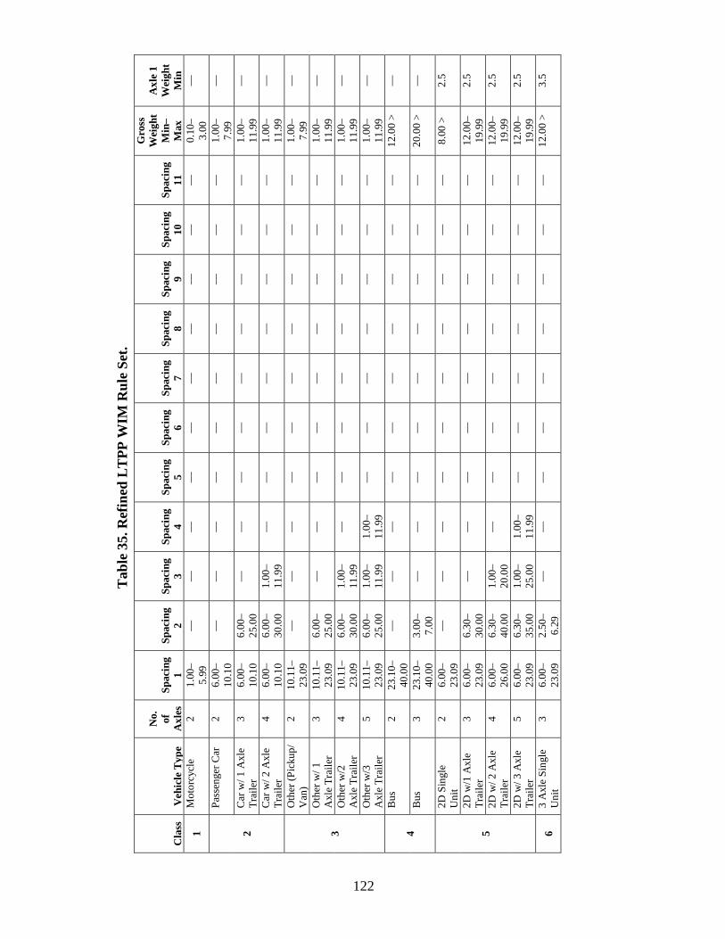
Tab

le 3

5. R

efin

ed L

TPP

WIM

Rul

e Se

t.

Cla

ss

Veh

icle

Typ

e

No.

of

A

xles

Sp

acin

g 1

Spac

ing

2 Sp

acin

g 3

Spac

ing

4 Sp

acin

g 5

Spac

ing

6 Sp

acin

g 7

Spac

ing

8 Sp

acin

g 9

Spac

ing

10

Spac

ing

11

Gro

ss

Wei

ght

Min

–M

ax

Axl

e 1

Wei

ght

Min

1 M

otor

cycl

e 2

1.00

–5.

99

—

—

—

—

—

—

—

—

—

—

0.10

–3.

00

—

2

Pass

enge

r Car

2

6.00

–10

.10

—

—

—

—

—

—

—

—

—

—

1.00

–7.

99

—

Car

w/ 1

Axl

e Tr

aile

r 3

6.00

–10

.10

6.00

–25

.00

—

—

—

—

—

—

—

—

—

1.00

–11

.99

—

Car

w/ 2

Axl

e Tr

aile

r 4

6.00

–10

.10

6.00

–30

.00

1.00

–11

.99

—

—

—

—

—

—

—

—

1.00

–11

.99

—

3

Oth

er (P

icku

p/

Van

) 2

10.1

1–23

.09

—

—

—

—

—

—

—

—

—

—

1.00

–7.

99

—

Oth

er w

/ 1

Axl

e Tr

aile

r 3

10.1

1–23

.09

6.00

–25

.00

—

—

—

—

—

—

—

—

—

1.00

–11

.99

—

Oth

er w

/2

Axl

e Tr

aile

r 4

10.1

1–23

.09

6.00

–30

.00

1.00

–11

.99

—

—

—

—

—

—

—

—

1.00

–11

.99

—

Oth

er w

/3

Axl

e Tr

aile

r 5

10.1

1–23

.09

6.00

–25

.00

1.00

–11

.99

1.00

–11

.99

—

—

—

—

—

—

—

1.00

–11

.99

—

4

Bus

2

23.1

0–40

.00

—

—

—

—

—

—

—

—

—

—

12.0

0 >

—

Bus

3

23.1

0–40

.00

3.00

–7.

00

—

—

—

—

—

—

—

—

—

20.0

0 >

—

5

2D S

ingl

e U

nit

2 6.

00–

23.0

9 —

—

—

—

—

—

—

—

—

—

8.

00 >

2.

5

2D w

/1 A

xle

Trai

ler

3 6.

00–

23.0

9 6.

30–

30.0

0 —

—

—

—

—

—

—

—

—

12

.00–

19.9

9 2.

5

2D w

/ 2 A

xle

Trai

ler

4 6.

00–

26.0

0 6.

30–

40.0

0 1.

00–

20.0

0 —

—

—

—

—

—

—

—

12

.00–

19.9

9 2.

5

2D w

/ 3 A

xle

Trai

ler

5 6.

00–

23.0

9 6.

30–

35.0

0 1.

00–

25.0

0 1.

00–

11.9

9 —

—

—

—

—

—

—

12

.00–

19.9

9 2.

5

6 3

Axl

e Si

ngle

U

nit

3 6.

00–

23.0

9 2.

50–

6.29

—

—

—

—

—

—

—

—

—

12

.00

> 3.

5

122

Class

Vehicle T

ype

No.

of A

xles Spacing

1 Spacing

2 Spacing

3 Spacing

4 Spacing

5 Spacing

6 Spacing

7 Spacing

8 Spacing

9 Spacing

10 Spacing

11

Gross

Weight

Min–

Max

Axle 1

Weight

Min

7

4 Axle Single

Unit

4 6.00–23.09

2.50–6.29

2.50–12.99

—

—

—

—

—

—

—

—

12.00 > 3.5

5 Axle Single

Unit

5 6.00–23.09

2.50–6.29

2.50–6.29

2.50–15.00

—

—

—

—

—

—

—

20.00 > 3.5

6 Axle Single

Unit

6 6.00–23.09

2.50–6.29

2.50–6.29

2.50–6.29

2.50–15.00

—

—

—

—

—

—

12.00 > 3.5

7 Axle Single

Unit

7 6.00–23.09

2.50–6.29

2.50–6.29

2.50–6.29

2.50–6.29

2.50–15.00

—

—

—

—

—

12.00 > 3.5

8

Semi, 2S1

3 6.00–23.09

11.00–45.00

—

—

—

—

—

—

—

—

—

20.00 > 3.5

Semi, 3S1

4 6.00–26.00

2.50–6.29

13.00–50.00

—

—

—

—

—

—

—

—

20.00 > 5

Semi, 2S2

4 6.00–26.00

8.00–45.00

2.50–20.00

—

—

—

—

—

—

—

—

20.00 > 3.5

9

Semi, 3S2

5 6.00–30.00

2.50–6.29

6.30–65.00

2.50–11.99

—

—

—

—

—

—

—

20.00 > 5

Truck+Full Trailer (3–2)

5 6.00–30.00

2.50–6.29

6.30–50.00

12.00–27.00

—

—

—

—

—

—

—

20.00> 3.5

Semi, 2S3

5 6.00–30.00

16.00–45.00

2.50–6.30

2.50–6.30

—

—

—

—

—

—

—

20.00 > 3.5

10

Semi, 3S3

6 6.00–26.00

2.50–6.30

6.10–45.00

2.50–11.99

2.50–10.99

—

—

—

—

—

—

20.00 > 5

Truck (3)/ trailer(4)

7 6.00–26.00

2.50–6.30

6.10–45.00

2.50–11.99

2.50–10.99

2.50–10.99

—

—

—

—

—

20.00 > 5


7 6.00–26.00

2.50–6.30

2.50–6.30

6.10–45.00

2.50–10.99

2.50–10.99

—

—

—

—

—

20.00 > 5


8 6.00–26.00

2.50–6.30

6.10–45.00

2.50–11.99

2.50–10.99

2.50–10.99

2.50–15.00

—

—

—

—

20.00 > 5


8 6.00–26.00

2.50–6.30

2.50–6.30

6.10–45.00

2.50–10.99

2.50–10.99

2.50–15.00

—

—

—

—

20.00 > 5

11 Sem

i+Full Trailer, 2S12

5 6.00–30.00

11.00–26.00

6.00–20.00

11.00–26.00

—

—

—

—

—

—

—

20.00 > 3.5

12 Sem

i+Full Trailer, 3S12

6 6.00–26.00

2.50–6.30

11.00–26.00

6.00–24.00

11.00–26.00

—

—

—

—

—

—

20.00 > 5

123

Cla

ss

Veh

icle

Typ

e

No.

of

A

xles

Sp

acin

g 1

Spac

ing

2 Sp

acin

g 3

Spac

ing

4 Sp

acin

g 5

Spac

ing

6 Sp

acin

g 7

Spac

ing

8 Sp

acin

g 9

Spac

ing

10

Spac

ing

11

Gro

ss

Wei

ght

Min

–M

ax

Axl

e 1

Wei

ght

Min

13

7 A

xle

Mul

ti’s

7 6.

00–

45.0

0 3.

00–

45.0

0 3.

00–

45.0

0 3.

00–

45.0

0 3.

00–

45.0

0 3.

00–

45.0

0 —

—

—

—

—

20

.00

> 5

8 A

xle

Mul

ti’s

8 6.

00–

45.0

0 3.

00–

45.0

0 3.

00–

45.0

0 3.

00–

45.0

0 3.

00–

45.0

0 3.

00–

45.0

0 3.

00–

45.0

0 —

—

—

—

20

.00

> 5

9 A

xle

Mul

ti’s

9 6.

00–

45.0

0 3.

00–

45.0

0 3.

00–

45.0

0 3.

00–

45.0

0 3.

00–

45.0

0 3.

00–

45.0

0 3.

00–

45.0

0 3.

00–

45.0

0 —

—

—

20

.00

> 5

10 A

xle

Mul

ti's

10

6.00

–45

.00

3.00

–45

.00

3.00

–45

.00

3.00

–45

.00

3.00

–45

.00

3.00

–45

.00

3.00

–45

.00

3.00

–45

.00

3.00

–45

.00

—

—

20.0

0 >

5

11 A

xle

Mul

ti's

11

6.00

–45

.00

3.00

–45

.00

3.00

–45

.00

3.00

–45

.00

3.00

–45

.00

3.00

–45

.00

3.00

–45

.00

3.00

–45

.00

3.00

–45

.00

3.00

–45

.00

—

20.0

0 >

5

12 A

xle

Mul

ti's

12

6.00

–45

.00

3.00

–45

.00

3.00

–45

.00

3.00

–45

.00

3.00

–45

.00

3.00

–45

.00

3.00

–45

.00

3.00

–45

.00

3.00

–45

.00

3.00

–45

.00

3.00

–45

.00

20.0

0 >

5

— In

dica

tes n

ot a

pplic

able

M

in =

Min

imum

M

ax =

Max

imum

124

APPENDIX A. VEHICLE CLASSIFICATION RULE SETS

This appendix contains the classification rules sets used in conducting this study. Table 36 presents the LTPP classification rule set for SPS WIM sites that was adopted in March 2006 by Traffic ETG. It was used as the baseline LTPP rule set. Table 37 and table 38 present data received for California from Caltrans delineating the Caltrans District 07 Classification Table by Number of Axles as of June 1996 and the California CALIF 4 WIM Classification Rule Set, respectively. Table 39 and table 40 are Florida’s Classification Rule Set and the Florida Department of Transportation’s Classifier Axle Spacing Rule Set, respectively. Table 41 is the Michigan Department of Transportation’s Classification and Weight Parameters for WIM. Table 42 is Minnesota’s Classification Rule Set Rule Table dated 2006. Table 43 and table 44 are Missouri’s and Ohio’s Classification Rule Sets, respectively. Following these tables is section that presents Virginia Department of Transportation’s Rule Set in the form of output from the State’s system. Table 45 presents output from Washington Department of Transportation’s system describing its classifications.

125

Tab

le 3

6. L

TPP

cla

ssifi

catio

n ru

le se

t for

SPS

WIM

site

s (ad

opte

d M

arch

200

6 by

Tra

ffic

ETG

).

Cla

ss

Veh

icle

Typ

e N

o. o

f A

xles

Sp

acin

g (ft

) Sp

acin

g 2

(ft)

Spac

ing

3 (f

t) Sp

acin

g 4

(ft)

Spac

ing

5 (f

t) Sp

acin

g 6

(ft)

Spac

ing

7 (f

t) Sp

acin

g 8

(ft)

Gro

ss W

eigh

t M

in–M

ax

(kip

s)

Axl

e 1

Wei

ght

Min

1

(kip

s)

1 M

otor

cycl

e

2

1.00

–5.9

9 —

—

—

—

—

—

—

0.

10–3

.00

—

2 Pa

ssen

ger C

ar

6.00

–10.

10

—

—

—

—

—

—

—

1.00

–7.9

9 —

3

Oth

er (P

icku

p/V

an)

10.1

1–23

.09

—

—

—

—

—

—

—

1.00

–7.9

9 —

4

Bus

23

.10–

40.0

0 —

—

—

—

—

—

—

12

.00

> —

5

2D S

ingl

e U

nit

6.00

–23.

09

—

—

—

—

—

—

—

8.00

>

2.5

2 C

ar w

ith1

Axl

e Tr

aile

r

3

6.00

–10.

10

6.00

–25.

00

—

—

—

—

—

—

1.00

–11.

99

—

3 O

ther

with

1 A

xle

Trai

ler

10.1

1–23

.09

6.00

–25.

00

—

—

—

—

—

—

1.00

–11.

99

—

4 B

us

23.1

0–40

.00

3.00

–7.0

0 —

—

—

—

—

—

20

.00

> —

5

2D w

ith 1

Axl

e Tr

aile

r 6.

00–2

3.09

6.

30–3

0.00

—

—

—

—

—

—

12

.00–

19.9

9 2.

5 6

3 A

xle

Sing

le U

nit

6.00

–23.

09

2.50

–6.2

9 —

—

—

—

—

—

12

.00

> 3.

5 8

Sem

i, 2S

1 6.

00–2

3.09

11

.00–

45.0

0 —

—

—

—

—

—

20

.00

> 3.

5 2

Car

with

2 A

xle

Trai

ler

4

6.00

–10.

10

6.00

–30.

00

1.00

–11.

99

—

—

—

—

—

1.00

–11.

99

—

3 O

ther

with

2 A

xle

Trai

ler

10.1

1–23

.09

6.00

–30.

00

1.00

–11.

99

—

—

—

—

—

1.00

–11.

99

—

5 2D

with

2 A

xle

Trai

ler

6.00

–26.

00

6.30

–40.

00

1.00

–20.

00

—

—

—

—

—

12.0

0–19

.99

2.5

7 4

Axl

e Si

ngle

Uni

t 6.

00–2

3.09

2.

50–6

.29

2.50

–12.

99

—

—

—

—

—

12.0

0 >

3.5

8 Se

mi,

3S1

6.00

–26.

00

2.50

–6.2

9 13

.00–

50.0

0 —

—

—

—

—

20

.00

> 5.

0 8

Sem

i, 2S

2 6.

00–2

6.00

8.

00–4

5.00

2.

50–2

0.00

—

—

—

—

—

20

.00

> 3.

5 3

Oth

er w

ith 3

Axl

e Tr

aile

r

5

10.1

1–23

.09

6.00

–25.

00

1.00

–11.

99

1.00

–11.

99

—

—

—

—

1.00

–11.

99

—

5 2D

with

3 A

xle

Trai

ler

6.00

–23.

09

6.30

–35.

00

1.00

–25.

00

1.00

–11.

99

—

—

—

—

12.0

0–19

.99

2.5

7 5

Axl

e Si

ngle

Uni

t 6.

00–2

3.09

2.

50–6

.29

2.50

–6.2

9 2.

50–6

.30

—

—

—

—

12.0

0 >

3.5

9 Se

mi,

3S2

6.00

–30.

00

2.50

–6.2

9 6.

30–6

5.00

2.

50–1

1.99

—

—

—

—

20

.00

> 5.

0 9

Truc

k+Fu

ll Tr

aile

r (3–

2)

6.00

–30.

00

2.50

–6.2

9 6.

30–5

0.00

12

.00–

27.0

0 —

—

—

—

20

.00>

3.

5 9

Sem

i, 2S

3 6.

00–3

0.00

16

.00–

45.0

0 2.

50–6

.30

2.50

–6.3

0 —

—

—

—

20

.00

> 3.

5 11

Se

mi+

Full

Trai

ler,

2S12

6.

00–3

0.00

11

.00–

26.0

0 6.

00–2

0.00

11

.00–

26.0

0 —

—

—

—

20

.00

> 3.

5 10

Se

mi,

3S3

6 6.

00–2

6.00

2.

50–6

.30

6.10

–50.

00

2.50

–11.

99

2.50

–10.

99

—

—

—

20.0

0 >

5.0

12

Sem

i+Fu

ll Tr

aile

r, 3S

12

6.00

–26.

00

2.50

–6.3

0 11

.00–

26.0

0 6.

00–2

4.00

11

.00–

26.0

0 —

—

—

20

.00

> 5.

0 13

7

Axl

e M

ulti

7 6.

00–4

5.00

3.

00–4

5.00

3.

00–4

5.00

3.

00–4

5.00

3.

00–4

5.00

3.

00–4

5.00

—

—

20

.00

> 5.

0 13

8

Axl

e M

ulti

8 6.

00–4

5.00

3.

00–4

5.00

3.

00–4

5.00

3.

00–4

5.00

3.

00–4

5.00

3.

00–4

5.00

3.

00–4

5.00

—

20

.00

> 5.

0 13

9

Axl

e M

ulti

9 6.

00–4

5.00

3.

00–4

5.00

3.

00–4

5.00

3.

00–4

5.00

3.

00–4

5.00

3.

00–4

5.00

3.

00–4

5.00

3.

00–4

5.00

20

.00

> 5.

0 1 Su

gges

ted

Axl

e 1

min

imum

wei

ght t

hres

hold

if a

llow

ed b

y W

IM sy

stem

’s c

lass

alg

orith

m p

rogr

amm

ing

— In

dica

tes n

ot a

pplic

able

M

ax =

Max

imum

M

in =

Min

imum

126

Table 37. C

altrans District 07 C

lassification Table by N

umber of A

xles (as of 6/96).N

o. of Axles

Class

Axle 1–2 (ft)

Axle 2–3 (ft)

Axle 3–4 (ft)

Axle 4–5 (ft)

Axle 5–6 (ft)

Axle 6–7 (ft)

Axle 7–8 (ft)

Axle 8–9 (ft)

2 1

00.1–06.1 —

—

—

—

—

—

—

2

2 06.1–10.0

—

—

—

—

—

—

—

2 3

10.0–14.5 —

—

—

—

—

—

—

2

4 23.1–40.0

—

—

—

—

—

—

—

2 5

14.5–23.1 —

—

—

—

—

—

—

3

2 06.1–10.0

06.0–25.0 —

—

—

—

—

—

3

3 10.0–14.5

06.0–25.0 —

—

—

—

—

—

3

4 23.1–40.0

03.5–06.0 —

—

—

—

—

—

3

6 06.1–23.1

03.5–06.0 —

—

—

—

—

—

3

8 06.1–23.0

11.0–40.0 —

—

—

—

—

—

4

2 06.1–10.0

06.0–25.0 01.0–12.0

—

—

—

—

—

4 3

10.0–14.5 06.0–25.0

01.0–12.0 —

—

—

—

—

4

7 06.1–23.1

03.5–06.0 03.5–13.0

—

—

—

—

—

4 8

06.1–23.0 03.5–06.0

06.1–44.0 —

—

—

—

—

4

8 06.1–23.0

11.0–44.0 03.5–12.0

—

—

—

—

—

5 3

10.0–14.5 06.0–25.0

01.0–03.5 01.0–03.5

—

—

—

—

5 9

06.1–26.0 03.5–06.0

06.1–46.0 03.5–10.9

—

—

—

—

5 11

06.1–26.0 11.1–26.0

06.1–20.0 11.1–26.0

—

—

—

—

5 14

06.1–23.0 03.5–06.0

06.1–23.0 11.0–27.0

—

—

—

—

6 10

06.1–26.0 03.5–06.0

06.1–46.0 00.1–11.0

00.1–11.0 —

—

—

6

12 06.1–26.0

03.5–06.0 11.1–26.0

06.1–24.0 11.1–26.0

—

—

—

7 13

06.1–45.0 03.5–45.0

03.5–45.0 03.5–45.0

03.5–45.0 03.5–45.0

—

—

8 13

06.1–45.0 03.5–45.0

03.5–45.0 03.5–45.0

03.5–45.0 03.5–45.0

03.5–45.0 —

13

06.1–45.0 03.5–45.0

03.5–45.0 03.5–45.0

03.5–45.0 03.5–45.0

03.5–45.0 03.5–45.0

Default C

lasses (for Vehicles T

hat Do N

ot Fit Into Table A

bove) N

o. of Axles

1 2

3 4

5 6

7 8

9 C

lass 2

2 15

15 15

15 15

15 15


127

Tab

le 3

8. C

alifo

rnia

CA

LIF

4 W

IM C

lass

ifica

tion

Rul

e Se

t.

Cla

ss

Veh

icle

Des

crip

tion

No.

of A

xles

Sp

acin

g 1–

2 (ft

) Sp

acin

g 2–

3 (ft

) Sp

acin

g 3–

4 (ft

) Sp

acin

g 4–

5 (ft

) Sp

acin

g 5–

6 (ft

) Sp

acin

g 6–

7 (ft

) Sp

acin

g 7–

8 (ft

) Sp

acin

g 8–

9 (ft

) W

eigh

t (ki

ps)

Min

–Max

1

Mot

orcy

cle

2 0.

10–5

.99

0.10

–3.0

0 2

Aut

o, P

icku

p 2

6.00

–9.9

9 1.

00–7

.99

2 A

uto

with

1 A

xle

Trlr

3 6.

00–9

.99

6.00

–25.

00

1.00

–11.

99

2 A

uto

with

2 A

xle

Trlr

4 6.

00–9

.99

6.00

–25.

00

1.00

–11.

99

1.00

–11.

99

3 O

ther

(Lim

o, V

an, R

V)

2 10

.00–

22.9

9 1.

00–7

.99

3 O

ther

with

1 A

xle

Trlr

3 10

.00–

16.0

0 6.

00–2

5.00

1.

00–1

1.99

3

Oth

er w

ith 2

Axl

e Tr

lr 4

10.0

0–16

.00

6.00

–25.

00

1.00

–11.

99

1.00

–11.

99

3 O

ther

with

3 A

xle

Trlr

5 10

.00–

16.0

0 6.

00–2

5.00

1.

00–3

.49

1.00

–3.4

9 1.

00–1

1.99

4

Bus

2

23.0

0–40

.00

12.0

0–>

4 B

us

3 23

.10–

40.0

0 3.

00–5

.99

20.0

0–>

5 2d

2

6.00

–22.

99

8.00

–>

5 2d

with

1 A

xle

Trlr

3 6.

00–2

3.09

6.

00–2

5.00

12

.00–

19.9

9 5

2d w

ith 2

Axl

e Tr

lr 4

6.00

–23.

09

6.00

–25.

00

1.00

–11.

99

12.0

0–19

.99

6 3

Axl

e 3

6.00

–23.

09

3.00

–5.9

9 12

.00–

> 7

4 A

xle

4 6.

00–2

3.09

3.

00–5

.99

3.00

–12.

99

12.0

0–>

8 2s

1, 2

1 3

6.00

–23.

00

11.0

0–40

.00

20.0

0–>

8 3s

1, 3

1 4

6.00

–23.

00

3.00

–5.9

9 13

.00–

44.0

0 12

.00–

> 8

2s2

4 6.

00–2

3.00

11

.00–

44.0

0 3.

00–1

1.99

20

.00–

> 9

3s2

5 6.

00–3

2.00

3.

00–5

.99

6.00

–46.

00

3.00

–10.

99

12.0

0–>

10

3s3,

33

6 6.

00–3

2.00

3.

00–5

.99

6.00

–46.

00

3.00

–11.

99

3.0–

10.9

9 12

.00–

> 11

2s

12

5 6.

00–2

6.00

11

.00–

26.0

0 6.

00–2

0.00

11

.00–

26.0

0 12

.00–

> 12

3s

12

6 6.

00–3

2.00

3.

00–5

.99

11.0

0–26

.00

6.00

–24.

00

11.0

0–26

.00

12.0

0–>

13

2s23

, 3s2

2, 3

s13

7 6.

00–4

5.00

3.

00–4

5.00

3.

00–4

5.00

3.

00–4

5.00

3.

00–4

5.00

3.

00–4

5.00

12

.00–

> 13

3s

23

8 6.

00–4

5.00

3.

00–4

5.00

3.

00–4

5.00

3.

00–4

5.00

3.

00–4

5.00

3.

00–4

5.00

3.

00–4

5.00

12

.00–

> 13

Pe

rmit

9 6.

00–4

5.00

3.

00–4

5.00

3.

00–4

5.00

3.

00–4

5.00

3.

00–4

5.00

3.

00–4

5.00

3.

00–4

5.00

3.

00–4

5.00

12

.00-

> 14

32

5

6.00

-26.

00

3.00

-5.9

9 6.

00-2

3.00

11

.00-

27.0

0 12

.00-

> 15

Er

ror a

nd/o

r Unc

lass

ified

—

V

ehic

les N

ot M

eetin

g A

xle

Con

figur

atio

ns S

et fo

r Cla

ssifi

catio

ns 1

Thr

ough

14

— In

dica

tes n

ot a

pplic

able

M

in =

Min

imum

M

ax =

Max

imum

Tr

lr =

Trai

ler

128

Table 39. Florida C

lassification Rule Set

Class

Vehicle T

ype

No.

of A

xles Spacing

1 to 2 (ft) Spacing

2 to 3 (ft) Spacing

3 to 4 (ft) Spacing

4 to 5 (ft) Spacing

5 to 6 (ft) Spacing

6 to 7 (ft) Spacing

7 to 8 (ft) Spacing

8 to 9 (ft)

Spacing 9 to 10

(ft)

Spacing 10 to 11

(ft)

Min

Axle 1

Weight for

LT

PP M

in–Max

GV

W

1 M

otorcycle 2

0.1–6.0 100 >

2 A

uto 2

6.01–10.0 1.0 K

> 3

Other(V

an, Pickup, Limo

2 10.01–13.0

1.0 K >

4 B

us 2

23.01–40.0 12.0 K

> 5

2 D

2 13.31–23.0

1.0 K >

2 A

uto 1 Axle Trlr

3 6.01–10.0

6.0–25.0 1.0 K

> 3

Other w

ith1 Axle Trlr

3 10.01–13.30

6.0–25.0 1.0 K

> 4

Bus

3 23.01–40.0

0.1 –6.0 12.0 K

> 5

2d with1 A

xle Trlr 3

13.31–23.0 6.0–25.0

1.0 K >

6 3 A

xle 3

6.01–23.0 0.1–5.99

12.0 K >

8 2S1, 21

3 6.01–23.0

11.0–40.0 12.0 K

> 2

Auto w

ith 2 Axle Trlr

4 6.01–10.0

6.0–25.0 0.1–6.0

1.0 K >

3 O

ther with 2 A

xle Trlr 4

10.01–13.30 6.0–25.0

0.1–6.0 1.0 K

> 5

2d with 2 A

xle Trlr 4

13.31–23.0 6.0–25.0

0.1–6.0 1.0 K

> 7

4 Axle

4 6.01–23.0

0.1–6.0 0.1–13.0

12.0 K >

8 3S1, 31

4 6.01–23.0

0.1–6.0 6.01–44.0

12.0 K >

8 2S2

4 6.01–23.0

11.0–40.0 0.1–10.99

12.0 K >

3 O

ther with 3 A

xle Trlr 5

10.01–13.3 6.0–25.0

0.1–6.0 0.1–6.0

1.0 K >

5 2d w

ith 3 Axle Trlr

5 13.31–23.0

6.0–25.0 0.1–6.0

0.1–6.0 1.0 K

> 9

3S2 5

6.01–26.0 0.1–6.0

6.01–46.0 0.1–10.99

12.0 K >

9 32

5 6.01–26.0

0.1–6.0 6.01–23.0

11.0–27.0 12.0 K

> 11

2S12 5

6.01–26.0 11.0–26.0

6.1–20.0 11.1–26.0

12.0 K >

10 3S3, 33

6 6.01–26.0

0.1–6.0 0.1–46.0

0.1–11.0 0.1–11.0

12.0 K >

12 2S12

6 6.01–26.0

0.1–6.0 11.1–26.0

6.01–24.0 11.1–26.0

12.0 K >

10 O

ther Class 10 V

ehicles 7

6.01–16.7 0.1–6.0

13.3–40.0 0.1–13.3

0.1–13.3 0.1–13.3

12.0 K >

13 2S23,3S22,3S13

7 1.0–45.0

1.0–45.0 1.0–45.0

1.0–45.0 1.0–45.0

1.0–45.0 12.0 K

> 13

3S23 8

1.0–45.0 1.0–45.0

1.0–45.0 1.0–45.0

1.0–45.0 1.0–45.0

1.0–45.0 12.0 K

> 13

Permit

9 1.0–45.0

1.0–45.0 1.0–45.0

1.0–45.0 1.0–45.0

1.0–45.0 1.0–45.0

1.0–45.0 12.0 K

> —

Indicates not applicable LTPP = Long-Term

Pavement Perform

ance G

VW

= Gross V

ehicle Weight

Min = M

inimum

M

ax = Maxim

um

Trlr = Trailer

129

Tab

le 4

0. F

lori

da D

epar

tmen

t of T

rans

port

atio

n C

lass

ifier

Axl

e Sp

acin

g R

ule

Set.

Ord

er

Cla

ss

Veh

icle

Des

crip

tion

No.

of A

xles

Sp

acin

g 1–

2 (f

t)

Spac

ing

2–3

(ft)

Sp

acin

g 3–

4 (f

t)

Spac

ing

4–5

(ft)

Sp

acin

g 5–

6 (f

t)

Spac

ing

6–7

(ft)

Sp

acin

g 7–

8 (f

t)

Spac

ing

8 -9

(f

t)

1 1

Mot

orcy

cle

2 0.

1–6.

0 —

—

—

—

—

—

—

2

2 A

uto,

Pic

kup

2 6.

00–1

0.0

—

—

—

—

—

—

—

3 3

Oth

er (L

imo,

Van

, RV

) 2

10.0

0–13

.30

—

—

—

—

—

—

—

4 4

Bus

2

23.0

0–40

.0

—

—

—

—

—

—

—

5 5

2 D

2

13.3

0–23

.0

—

—

—

—

—

—

—

1 8

2S1,

21

3 10

.00–

23.0

11

.0–4

0.0

—

—

—

—

—

—

2 4

Bus

3

23.0

0–40

.0

0.1–

6.0

—

—

—

—

—

—

3 6

3 A

xle

3 6.

00–2

3.0

0.1–

6.0

—

—

—

—

—

—

4 3

Oth

er w

ith 1

Axl

e Tr

lr 3

10.0

0–13

.30

6.0–

25.0

—

—

—

—

—

—

5

2 A

uto

with

1 A

xle

Trlr

3 6.

00–1

0.0

6.0–

25.0

—

—

—

—

—

—

6

5 2D

with

1 A

xle

Trlr

3 13

.30–

23.0

6.

0–25

.0

—

—

—

—

—

—

1 8

2S2

4 10

.00–

23.0

11

.0–4

0.0

2.0–

12.0

—

—

—

—

—

2

8 3S

1, 3

1 4

6.00

–23.

0 0.

1–6.

0 6.

00–4

4.0

—

—

—

—

—

3 7

4 A

xle

4 6.

00–2

3.0

0.1–

6.0

0.1–

6.0

—

—

—

—

—

4 3

Oth

er w

ith 2

Axl

e Tr

lr 4

10.0

0–13

.30

6.0–

25.0

0.

1–6.

0 —

—

—

—

—

5

5 2D

with

2 A

xle

Trlr

4 13

.30

-23.

0 6.

0–25

.0

0.1–

6.0

—

—

—

—

—

6 2

Aut

o w

ith 2

Axl

e Tr

lr 4

6.00

–10.

0 6.

0–25

.0

0.1–

6.0

—

—

—

—

—

1 9

3S2

5 6.

00–2

6.0

0.1–

6.0

6.00

–46.

0 0.

1–11

.00

—

—

—

—

2 9

32

5 6.

00–2

6.0

0.1–

6.0

6.00

- 23.

0 11

.0–2

7.0

—

—

—

—

3 11

2S

12

5 6.

00–2

6.0

11.0

–26.

0 6.

00–2

0.0

11.0

0–26

.0

—

—

—

—

4 3

Oth

er w

ith 3

Axl

e Tr

lr 5

10.0

0–13

.30

6.0–

25.0

0.

1–6.

0 0.

1–6.

0 —

—

—

—

5

5 2D

with

3 A

xle

Trlr

5 13

.30–

23.0

6.

0–25

.0

0.1–

6.0

0.1–

6.0

—

—

—

—

1 10

3S

3, 3

3 6

6.00

–26.

0 0.

1–6.

0 0.

1–46

.0

0.1–

11.0

0.

1–11

.0

—

—

—

2 12

3S

12

6 6.

00–2

6.0

0.1–

6.0

11.0

0–26

.0

6.00

–24.

0 11

.00–

26.0

—

—

—

1

10

Oth

er C

lass

10

Veh

icle

s 7

6.00

–16.

7 0.

1–6.

0 13

.3–4

0.0

0.1–

13.3

0.

1–13

.3

0.1–

13.3

—

—

2

13

2S23

,3S2

2,3S

13

7 1.

0–45

.0

1.0–

45.0

1.

0–45

.0

1.0–

45.0

1.

0–45

.0

1.0–

45.0

—

—

1

13

3S23

8

1.0–

45.0

1.

0–45

.0

1.0–

45.0

1.

0–45

.0

1.0–

45.0

1.

0–45

.0

1.0–

45.0

—

1

13

Perm

it 9

1.0–

45.0

1.

0–45

.0

1.0–

45.0

1.

0–45

.0

1.0–

45.0

1.

0–45

.0

1.0–

45.0

1.

0–45

.0

15

Erro

r/Unc

lass

ified

—

—

—

—

—

—

—

—

—

—

Indi

cate

s not

app

licab

le

Trlr

= Tr

aile

r

130

Ta ble 41. M

ichigan Departm

ent of Transportation C

lassification and Weight Param

eters for WIM

Class

Vehicle

Description

No. of

Axles

Spacing 1 (ft)

Spacing 2 (ft)

Spacing 3 (ft)

Spacing 4 (ft)

Spacing 5 (ft)

Spacing 6 (ft)

Spacing 7 (ft)

Spacing 8 (ft)

Spacing 9 (ft)

Spacing 10 (ft)

Weight

Min–M

ax 1

Motorcycle

2 0.1–6.0

—

—

—

—

—

—

—

—

—

100–3,000 2

Car

2 6.0–10.1

—

—

—

—

—

—

—

—

—

1,000–8,000 3

Truck 2

10.1–16.0 —

—

—

—

—

—

—

—

—

1,000–8,000

4 B

us 2

21.09–40.0

—

—

—

—

—

—

—

—

—

12,000 > 5

2D

2 8.0–21.09

—

—

—

—

—

—

—

—

—

8,000 >

2 C

ar/1 Axle

Trailer 3

6.0–10.1 6.0–30.0

—

—

—

—

—

—

—

—

1,000–12,000

3 Truck/1 A

xle Trailer

3 10.1–16.0

6.0–30.0 —

—

—

—

—

—

—

—

1,000–15,000

4 B

us 3

21.09–40 3.0–7.0

—

—

—

—

—

—

—

—

20,000 >

5 2D

/1 Axle

Trailer 3

8.0–21.09 6.3–30.0

—

—

—

—

—

—

—

—

15,000–12,000

6 3 A

xle Single U

nit 3

8.0–26.0 2.5–6.3

—

—

—

—

—

—

—

—

12,000 > 8

Semi 2–1

3 8.0–23.09

11.0–40.0 —

—

—

—

—

—

—

—

20,000 >

2 C

ar/2 Axle

Trailer 4

6.0–10.1 6.0–30.0

1.0–11.99 —

—

—

—

—

—

—

1,000–12,000

3 Truck/2 A

xle Trailer

4 10.1–16.0

6.0–30.0 1.0–11.99

—

—

—

—

—

—

—

1,000–15,000

5 2D

/2 Axle

Trailer 4

8.0–23.09 6.3–30.0

1.0–11.99 —

—

—

—

—

—

—

15,000–20,000

7 4 A

xle Single U

nit 4

8.0–23.09 2.5–6.3

2.5–13.0 —

—

—

—

—

—

—

12,000 >

8 Sem

i 2–2 4

8.0–23.09 11.0–45.0

2.5–11.99 —

—

—

—

—

—

—

20,000 >

8 Sem

i 3–1 4

8.0–26.00 2.5–6.3

6.1–45.0 —

—

—

—

—

—

—

20,000 >

3 Truck/3 A

xle Trailer

5 10.1–16.0

6.0–30.0 1.0–11.99

1.0–11.99 —

—

1,000–15,000

7 5 A

xle Single U

nit 5

8.0–23.09 2.5–6.3

2.5–6.3 2.5–6.3

—

—

—

—

—

—

12,000 > 9

Semi 3–2

5 8.0–26.0

2.5–6.3 6.0–45.0

2.5–27.0 —

—

—

—

—

—

20,000 >

9 Sem

i 2–3 5

8.0–23.09 11.0–45.0

2.5–6.3 2.5–6.3

—

—

—

—

—

—

20,000 > 11

Semi 2–1–2

5 8.0–26.0

11.0–26.0 6.0–20.0

11.0–26.0 —

—

—

—

—

—

12,000 >

10 Sem

i 3–3 6

8.0–26.0 2.5–6.3

6.1–45.0 2.5–11.99

2.5–11.99 —

—

—

—

—

20,000 >

10 Sem

i 2–4 6

8.0–23.09 11.0–45.0

2.5–6.3 2.5–6.3

2.5–6.3 —

—

—

—

—

20,000 >

10 Sem

i 4–2 6

8.0–26.0 2.5–6.3

2.5–6.3 6.1–46.0

2.5–11.99 —

—

—

—

—

20,000 >

12 Sem

i 3–1–2 6

8.0–26.0 2.5–6.3

11.0–26.0 6.0–24.0

11.0–26.0 —

—

—

—

—

12,000 >

10 Sem

i 3–4 7

8.0–26.0 2.5–6.3

10.0–20.0 6.0–12.0

6.0–12.0 6.0–12.0

—

—

—

20,000 > 10

Semi 3–4

7 8.0–26.0

2.5–6.3 3.5–45.0

2.5–12.0 2.5–6.3

2.5–6.3 —

—

—

20,000 >

13 Sem

i 3–*–* 7

8.0–45.0 3.0–45.0

3.0–45.0 3.0–45.0

3.0–45.0 3.0–45.0

—

—

—

20,000 > 10

Semi 3–5

8 8.0–26.0

2.5–6.3 3.5–45.0

2.5–6.3 2.5–6.3

2.5–6.3 2.5–6.3

—

—

20,000 > 10

Semi 3–5

8 8.0–26.0

2.5–6.3 10.0–20.0

6.0–12.0 2.5–6.3

2.5–6.3 2.5–6.3

—

—

20,000 > 13

Semi 3–*–*

8 8.0–45.0

3.0–45.0 3.0–45.0

3.0–45.0 3.0–45.0

3.0–45.0 3.0–45.0

—

—

—

20,000 > 10

Semi 3–6

9 8.0–26.0

2.5–6.3 3.5–45.0

2.5–6.3 2.5–6.3

2.5–6.3 2.5–6.3

2.5–6.3 —

—

20,000 >

131

Cla

ss

Veh

icle

D

escr

iptio

n N

o. o

f A

xles

Sp

acin

g 1

(ft)

Sp

acin

g 2

(ft)

Sp

acin

g 3

(ft)

Sp

acin

g 4

(ft)

Sp

acin

g 5

(ft)

Sp

acin

g 6

(ft)

Sp

acin

g 7

(ft)

Sp

acin

g 8

(ft)

Sp

acin

g 9

(ft)

Sp

acin

g 10

(ft)

Wei

ght

Min

–Max

10

Se

mi 3

–6

9 8.

0–26

.0

2.5–

6.3

10.0

–20.

0 6.

0–12

.0

2.5–

6.3

2.5–

6.3

2.5–

6.3

2.5–

6.3

—

—

20,0

00 >

10

Se

mi 4

–5

9 8.

0–26

.0

2.5–

6.3

2.5–

6.3

6.3–

15.0

2.

5–6.

3 2.

5–6.

3 2.

5–6.

3 2.

5–6.

3 —

—

20

,000

> 13

Se

mi 3

–*–*

9

8.0–

45.0

3.

0–45

.0

3.0–

45.0

3.

0–45

.0

3.0–

45.0

3.

0–45

.0

3.0–

45.0

3.

0–45

.0

—

—

20,0

00 >

10

Se

mi 3

–7

10

8.0–

26.0

2.

5–6.

3 3.

5–45

.0

2.5–

6.3

2.5–

6.3

2.5–

6.3

2.5–

6.3

2.5–

6.3

2.5–

6.3

—

20,0

00 >

10

Se

mi 3

–7

10

8.0–

26.0

2.

5–6.

3 10

.0–2

0.0

6.0–

12.0

2.

5–6.

3 2.

5–6.

3 2.

5–6.

3 2.

5–6.

3 2.

5–6.

3 —

20

,000

>

10

Sem

i 4–6

10

8.

0–26

.0

2.5–

6.3

2.5–

6.3

6.3–

15.0

2.

5–6.

3 2.

5–6.

3 2.

5–6.

3 2.

5–6.

3 2.

5–6.

3 —

20

,000

> 10

Se

mi 5

–5

10

8.0–

26.0

2.

5–6.

3 2.

5–6.

3 2.

5–6.

3 6.

3–15

.0

2.5–

6.3

2.5–

6.3

2.5–

6.3

2.5–

6.3

—

20,0

00>

13

Sem

i 3–*

–*

10

8.0–

45.0

3.

0–45

.0

3.0–

45.0

3.

0–45

.0

3.0–

45.0

3.

0–45

.0

3.0–

45.0

3.

0–45

.0

3.0–

45.0

—

20

,000

>

10

Sem

i 3–8

11

8.

0–26

.0

2.5–

6.3

3.5–

45.0

2.

5–6.

3 2.

5–6.

3 2.

5–6.

3 2.

5–6.

3 2.

5–6.

3 2.

5–6.

3 2.

5–6.

3 20

,000

>

10

Sem

i 3–8

11

8.

0–26

.0

2.5–

6.3

10.0

–20.

0 6.

0–12

.0

2.5–

6.3

2.5–

6.3

2.5–

6.3

2.5–

6.3

2.5–

6.3

2.5–

6.3

20,0

00 >

10

Se

mi 5

–6

11

8.0–

26.0

2.

5–6.

3 2.

5–6.

3 2.

5–6.

3 6.

3–15

.0

2.5–

6.3

2.5–

6.3

2.5–

6.3

2.5–

6.3

2.5–

6.3

20,0

00>

13

Sem

i 3–*

–*

11

8.0–

45.0

3.

0–45

.0

3.0–

45.0

3.

0–45

.0

3.0–

45.0

3.

0–45

.0

3.0–

45.0

3.

0–45

.0

3.0–

45.0

3.

0–45

.0

20,0

00 >

*A

ny n

umbe

r may

be

inse

rted

here

as l

ong

as th

e su

m o

f the

num

bers

subs

titut

ed fo

r the

two

aste

risks

(whi

ch c

an b

e di

ffere

nt fr

om e

ach

othe

r) p

lus t

he le

adin

g va

lue

equa

ls th

e to

tal n

umbe

r of

axle

s sho

wn

in th

e th

ird c

olum

n.

— In

dica

tes n

ot a

pplic

able

M

in =

Min

imum

M

ax =

Max

imum

132

Tab le 42. M

innesota Classification R

ule Set Rule T

able (2006)

nRuleNum

nAxleCount

nClass

1 to 2 Min

1 to 2 Max

2 to 3 Min

2 to 3 Max

3 to 4 Min

3 to 4 Max

4 to 5 Min

4 to 5 Max

5 to 6 Min

5 to 6 Max

6 to 7 Min

6 to 7 Max

7 to 8 Min

7 to 8 Max

8 to 9 Min

8 to 9 Max

9 to 10 Min

9 to 10 Max

10 to 11 Min

10 to 11 Max

11 to 12 Min

11 to 12 Max

1 2

1 12

90 0

0 0

0 0

0 0

0 0

0 0

0 0

0 0

0 0

0 0

0 2

2 2

91 121

0 0

0 0

0 0

0 0

0 0

0 0

0 0

0 0

0 0

0 0

3 2

3 121

163 0

0 0

0 0

0 0

0 0

0 0

0 0

0 0

0 0

0 0

0 4

2 5

163 288

0 0

0 0

0 0

0 0

0 0

0 0

0 0

0 0

0 0

0 0

5 2

4 288

481 0

0 0

0 0

0 0

0 0

0 0

0 0

0 0

0 0

0 0

0 6

3 6

121 266

24 72

0 0

0 0

0 0

0 0

0 0

0 0

0 0

0 0

0 0

7 3

1 12

90 12

96 0

0 0

0 0

0 0

0 0

0 0

0 0

0 0

0 0

0 8

3 2

91 121

36 241

0 0

0 0

0 0

0 0

0 0

0 0

0 0

0 0

0 0

9 3

5 163

288 72

245 0

0 0

0 0

0 0

0 0

0 0

0 0

0 0

0 0

0 10

3 3

121 163

72 265

0 0

0 0

0 0

0 0

0 0

0 0

0 0

0 0

0 0

11 3

8 108

289 264

481 0

0 0

0 0

0 0

0 0

0 0

0 0

0 0

0 0

0 12

3 4

288 481

36 481

0 0

0 0

0 0

0 0

0 0

0 0

0 0

0 0

0 0

13 4

7 72

266 12

72 12

97 0

0 0

0 0

0 0

0 0

0 0

0 0

0 0

0 14

4 2

12 121

72 241

12 241

0 0

0 0

0 0

0 0

0 0

0 0

0 0

0 0

16 4

3 121

163 72

301 12

241 0

0 0

0 0

0 0

0 0

0 0

0 0

0 0

0 17

4 8

132 164

12 72

12 481

0 0

0 0

0 0

0 0

0 0

0 0

0 0

0 0

18 4

8 132

164 241

481 40

97 0

0 0

0 0

0 0

0 0

0 0

0 0

0 0

0 19

4 4

121 289

12 72

97 241

0 0

0 0

0 0

0 0

0 0

0 0

0 0

0 0

20 4

4 156

266 72

361 12

241 0

0 0

0 0

0 0

0 0

0 0

0 0

0 0

0 21

4 4

288 481

24 481

12 481

0 0

0 0

0 0

0 0

0 0

0 0

0 0

0 0

22 5

3 72

163 72

301 12

36 12

36 0

0 0

0 0

0 0

0 0

0 0

0 0

0 23

5 4

72 266

12 72

72 133

36 97

0 0

0 0

0 0

0 0

0 0

0 0

0 0

24 5

7 72

234 12

72 36

72 36

97 0

0 0

0 0

0 0

0 0

0 0

0 0

0 25

5 7

121 266

12 72

12 97

97 241

0 0

0 0

0 0

0 0

0 0

0 0

0 0

26 5

9 72

234 72

481 36

97 36

97 0

0 0

0 0

0 0

0 0

0 0

0 0

0 27

5 9

72 301

36 72

133 541

36 181

0 0

0 0

0 0

0 0

0 0

0 0

0 0

28 5

11 72

234 181

301 72

241 181

301 0

0 0

0 0

0 0

0 0

0 0

0 0

0 29

6 4

72 266

12 72

12 301

96 301

12 241

0 0

0 0

0 0

0 0

0 0

0 0

30 6

4 121

266 24

61 97

219 24

61 24

61 0

0 0

0 0

0 0

0 0

0 0

0 31

6 7

72 266

12 72

12 97

12 97

12 97

0 0

0 0

0 0

0 0

0 0

0 0

32 6

10 72

301 36

73 218

481 36

181 36

97 0

0 0

0 0

0 0

0 0

0 0

0 33

6 12

96 481

12 97

96 541

12 97

97 481

0 0

0 0

0 0

0 0

0 0

0 0

34 7

7 72

234 12

72 12

97 12

97 12

97 12

97 0

0 0

0 0

0 0

0 0

0 35

7 10

72 301

36 73

96 541

36 181

36 97

36 97

0 0

0 0

0 0

0 0

0 0

36 7

13 96

481 12

97 96

481 12

97 96

481 97

481 0

0 0

0 0

0 0

0 0

0 N

ote: The maxim

um (M

ax) and minim

um (M

in) ranges are all in units of inches. M

in = Minim

um

Max = M

aximum

133

Tab

le 4

3. M

isso

uri C

lass

ifica

tion

Rul

e Se

t

Typ

e C

lass

N

o. o

f Axl

es

Axl

e 12

A

xle

2–3

Axl

e 3–

4 A

xle

4–5

Axl

e 5–

6 A

xle

6–7

Axl

e 7–

8 M

in

Max

M

in

Max

M

in

Max

M

in

Max

M

in

Max

M

in

Max

M

in

Max

A

15

0

Def

ault

—

—

—

—

Ove

rlap

on a

ll sp

acin

gs

—

—

—

—

B 2

1 D

efau

lt —

—

—

—

N

ot re

quire

d?

—

—

—

—

—

—

C 1

2 0.

1 6.

0 —

—

—

—

—

—

—

—

—

—

—

—

D

2

2 6.

0 10

.2

—

—

—

—

—

—

—

—

—

—

—

—

E 3

2 10

.2

13.5

—

—

—

—

—

—

—

—

—

—

—

—

F

5 2

13.5

22

.0

—

—

—

—

—

—

—

—

—

—

—

—

G

4 2

22.0

40

.0

—

—

—

—

—

—

—

—

—

—

—

—

H

2 2

Def

ault

—

—

—

—

—

—

—

—

—

—

—

—

—

I 2

3 6.

0 10

.2

6.0

23.0

L,

M

—

—

—

—

—

—

—

—

J 3

3 10

.2

13.5

6.

0 21

.0

—

—

—

—

—

—

—

—

—

—

K

5 3

13.5

22

.0

6.0

21.0

—

—

—

—

—

—

—

—

—

—

L

6 3

6.0

23.0

0.

1 8.

0 —

I,

J, K

—

—

—

—

—

—

—

—

M

8

3 6.

0 17

.0

14.0

40

.0

—

I, J,

K

—

—

—

—

—

—

—

—

N

4 3

22.0

40

.0

0.1

6.0

—

—

—

—

—

—

—

—

—

—

O

2 3

Def

ault

—

—

—

—

—

—

—

—

—

—

—

—

—

P 2

4 6.

0 10

.2

6.0

13.0

3.

2 13

.5

—

—

—

—

—

—

—

—

Q

2 4

6.0

10.2

6.

0 23

.0

0.1

3.2

—

—

—

—

—

—

—

—

R 3

4 10

.2

13.5

6.

0 13

.0

3.2

13.5

—

—

—

—

—

—

—

—

S

3 4

10.2

13

.5

6.0

35.0

0.

1 3.

2 —

—

—

—

—

—

—

—

T

4 4

22.0

40

.0

15.0

24

.0

6.0

16.0

—

—

—

—

—

—

—

—

U

5

4 13

.5

22.0

6.

0 40

.0

0.1

3.2

—

—

—

—

—

—

—

—

V

5 4

13.5

22

.0

6.0

40.0

6.

0 16

.0

—

—

—

—

—

—

—

—

W

7 4

6.0

23.0

0.

1 6.

0 0.

1 9.

0 —

X

—

—

—

—

—

—

X

8

4 6.

0 20

.0

0.1

6.0

6.0

40.0

—

W

—

—

—

—

—

—

Y

8

4 6.

0 17

.0

14.0

40

.0

3.2

6.0

—

—

—

—

—

—

—

—

Z 8

4 D

efau

lt —

—

—

—

—

—

—

—

—

—

—

—

—

A

A

4 5

22.0

40

.0

0.1

6.0

15.0

24

.0

6.0

16.0

—

—

—

—

—

—

A

B

9 5

6.0

22.0

0.

1 6.

0 6.

1 40

.0

0.1

11.5

A

C

—

—

—

—

AC

9

5 6.

0 22

.0

0.1

6.0

6.1

23.0

1.

1 23

.0

AB

—

—

—

—

A

D

11

5 6.

0 17

.0

11.1

25

.0

6.1

18.0

11

.1

25.0

—

—

—

—

—

—

A

E 9

5 D

efau

lt —

—

—

—

—

—

—

—

—

—

—

—

—

A

F 10

6

6.0

22.0

0.

1 6.

0 0.

1 40

.0

0.1

11.0

0.

1 11

.0

—

—

—

—

AG

12

6

6.0

22.0

0.

1 6.

0 1.

1 25

.0

6.1

18.0

11

.1

25.0

—

—

—

—

A

H

10

6 D

efau

lt —

—

—

—

—

—

—

—

—

—

—

—

—

A

I 13

7

0.1

40.0

0.

1 40

.0

0.1

40.0

0.

1 40

.0

0.1

40.0

0.

1 40

.0

—

—

AJ

13

7 D

efau

lt —

—

—

—

—

—

—

—

—

—

—

—

—

A

K

13

8 0.

1 40

.0

0.1

40.0

0.

1 40

.0

0.1

40.0

0.

1 40

.0

0.1

40.0

0.

1 40

.0

AL

13

8 D

efau

lt —

—

—

—

—

—

—

—

—

—

—

—

—

A

M

15

9 D

efau

lt —

—

—

—

—

—

—

—

—

—

—

—

—

A

N

15

10

Def

ault

—

—

—

—

—

—

—

—

—

—

—

—

—

AO

15

11

D

efau

lt —

—

—

—

—

—

—

—

—

—

—

—

—

A

P 15

12

D

efau

lt —

—

—

—

—

—

—

—

—

—

—

—

—

A

Q

15

13

Def

ault

—

—

—

—

—

—

—

—

—

—

—

—

—

AR

15

14

D

efau

lt —

—

—

—

—

—

—

—

—

—

—

—

—

A

S 15

15

D

efau

lt —

—

—

—

—

—

—

—

—

—

—

—

—

—

Indi

cate

s not

app

licab

le

Min

= M

inim

um

Max

= M

axim

um

134

Ta ble 44. O

hio Classification R

ule Set

Class

FHW

A M

odified Scheme F

Vehicle D

escription A

xles A

xle Space Betw

een Axle N

umbers (ft )

A–B

B–C

C

–D

D–E

E–F

F–G

G–H

H

–I I–J

J–K

K–L

L–M

...

T–U

1

Motorcycles

2 1–5.9

—

—

—

—

—

—

—

—

—

—

—

—

—

2 Passenger C

ars 2

6.0–10.2 —

—

—

—

—

—

—

—

—

—

—

—

—

2

Any 2 axle vehicles

2 1.0–45.0

—

—

—

—

—

—

—

—

—

—

—

—

—

2 Passenger C

ars w/1 axle trailer

3 6.0–10.2

6.0–18 —

—

—

—

—

—

—

—

—

—

—

—

2

Passenger Cars w

/2 axle trailer 4

6.0–10.2 6.0–18

1.0–6.0 —

—

—

—

—

—

—

—

—

—

—

3

Other(Lim

o, Van, R

V)

2 10.3–13.0

—

—

—

—

—

—

—

—

—

—

—

—

—

3 O

ther w/1 A

xle trailer 3

10.3–13.0 6.0–18

—

—

—

—

—

—

—

—

—

—

—

—

3 O

ther w/2 A

T 4

10.3–13.0 6.0–18

1.0–6.0 —

—

—

—

—

—

—

—

—

—

—

3

Other w

/3 AT

5 10.3–13.0

6.0–18 1.0–6.0

1.0–6.0 —

—

—

—

—

—

—

—

—

—

4

Bus w

/ 2 Axles

2 23.1–40

—

—

—

—

—

—

—

—

—

—

—

—

4 B

us w/ 3 A

xles 3

23.1–40 1.0–6.0

—

—

—

—

—

—

—

—

—

—

—

—

4 A

ny 3 axle vehicles 3

1.0–45.0 1.0–45.0

—

—

—

—

—

—

—

—

—

—

—

—

5 2 A

xle, Six Tire, Single U

nit Trucks 2

13.1–23.0 —

—

—

—

—

—

—

—

—

—

—

—

—

6 3 A

xle, Single Unit Trucks

3 6.10–23.0

1.0–6.0 —

—

—

—

—

—

—

—

—

—

—

—

7

4 Axle, Single U

nit Trucks 4

6.10–23 1.0–6.0

1.0–13.0 —

—

—

—

—

—

—

—

—

—

—

7

4 Axle, Single U

nit Trucks 4

6.10–23 8.0–20.0

1.0–6.0 —

—

—

—

—

—

—

—

—

—

—

7

5 Axle, Single U

nit Trucks 5

6.10–23 1.0–6.0

1.0–6.0 1.0–13.0

—

—

—

—

—

—

—

—

—

—

7 6 A


6 6.10–23

1.0–6.0 1.0–6.0

1.0–6.0 1.0–13.0

—

—

—

—

—

—

—

—

—

7 7 A


7 6.10–23

1.0–6.0 1.0–6.0

1.0–6.0 1.0–6.0

1.0–6.0 —

—

—

—

—

—

—

—

8

3 Axle, Single Trailer Trucks

3 6.10–22

11.0–40 —

—

—

—

—

—

—

—

—

—

—

8

4 Axle, Single Trailer Trucks

4 6.10–22

11.0–44 3.5–12.0

—

—

—

—

—

—

—

—

—

—

—

8 4 A

xle, Single Trailer Trucks 4

6.10–22 1.0–6.0

6.1–44 —

—

—

—

—

—

—

—

—

—

—

8

Any 4 axle vehicles

4 1.0–45.0

1.0–45.0 1.0–45.0

—

—

—

—

—

—

—

—

—

—

—

9 5 A


6.10–24.5 1.0–6.0

6.1–46.0 1.0–13

—

—

—

—

—

—

—

—

—

—

9 5 A


6.10–24.5 15.0–25

1.0–6.0 1.0–6.0

—

—

—

—

—

—

—

—

—

—

9 A


1.0–45.0 1.0–45.0

1.0–45.0 1.0–45.0

—

—

—

—

—

—

—

—

—

—

10 6 A


6.10–23 1.0–6.0

6.1–46.0 1–11.0

1–11.0 —

—

—

—

—

—

—

—

—

10

Any 6 axle vehicles

6 1.0–45.0

1.0–45.0 1.0–45.0

1.0–45.0 1.0–45.0

—

—

—

—

—

—

—

—

—

10 7 A


6.10–23 1.0–6.0

6.1–30 1.0–6.0

1.0–6.0 1.0–6.0

—

—

—

—

—

—

—

—

10 7 A


6.10–23 1.0–6.0

1.0–6.0 6.1–46

1.0–6.0 1.0–6.0

—

—

—

—

—

—

—

—

11 5 or less A

xle, Single Trailer Trucks

5 6.10–23

11.1–30 6.1–20

11.1–30 —

—

—

—

—

—

—

—

—

—

12 6 A

xle, Multi Trailer Trucks

6 6.10–23

1.0–6.0 11.1–26

6.1–18 11.1–26

—

—

—

—

—

—

—

—

—

13 7 A


7 6.10–23

1.0–6.0 11.1–26

1.0–6.0 6.1–20

11.1–26 —

—

—

—

—

—

—

—

13

7 Axle, M

ulti Trailer Trucks 7

6.10–23 1.0–6.0

11.1–26 6.1–20

6.1–26 1.0–6.0

—

—

—

—

—

—

—

—

13 A


1.0–45.0 1.0–45.0

1.0–45.0 1.0–45.0

1.0–45.0 1.0–45.0

—

—

—

—

—

—

—

—

13 8 A


8 6.10–23

1.0–6.0 11.1–26

1.0–6.0 6.1–20

11.1–26 1.0–6.0

—

—

—

—

—

—

—

13 9 A


9 6.10–23

1.0–6.0 11.1–26

1.0–6.0 6.1–20

11.1–26 6.1–20

11.1–26 —

—

—

—

—

—

14

Michigan G

rain Train 8

6.1–23 1.0–6.0

1.0–20 1.0–20

1.0–20 1.0–20

1.0–20 —

—

—

—

—

—

14

Michigan G

rain Train 9

6.1–23 1.0–6.0

1.0–20 1.0–20

1.0–20 1.0–20

1.0–20 1.0–20

—

—

—

—

—

—

14 M

ichigan Grain Train

10 6.1–23

1.0–6.0 1.0–20

1.0–20 1.0–20

1.0–20 1.0–20

1.0–20 1.0–20

—

—

—

—

—

14 M

ichigan Grain Train

11 6.1–23

1.0–6.0 1.0–20

1.0–20 1.0–20

1.0–20 1.0–20

1.0–20 1.0–20

1.0–20 —

—

—

—

15

Other

12–21 1–45

1–45 1–46

1–46 1–45

1–45 1–45

1–45 1–45

1–45 1–45

1–45 ...

1–45 —

Indicates not applicable

135

Virginia Department of Transportation Rule Set

Peek ADR Classification Editor Virginia DOT (2006).txt Tree name: PC042106, Description: ADR VDOT Piezo

0 axle vehicles. Default class = 21 Class 20: Length: 22 Feet to 100 Feet Class 19: Length: 17.4 Feet to 22 Feet Class 18: Length: 7 Feet to 17.4 Feet

1 axle vehicles. Default class = 21 Class 20: Length: 22 Feet to 100 Feet Class 17: Length: 17.4 Feet to 22 Feet Class 16: Length: 7 Feet to 17.4 Feet

2 axle vehicles. Default class = 15 Class 5: Axle Spacing: 14.7 Feet to 20 Feet Class 4: Axle Spacing: 20 Feet to 32 Feet Class 3: Axle Spacing: 10.2 Feet to 14.7 Feet Class 2: Axle Spacing: 6 Feet to 10.2 Feet Class 1: Axle Spacing: 2 Feet to 6 Feet

3 axle vehicles. Default class = 15 Class 8: Axle Spacing: 6 Feet to 14.7 Feet, 21 Feet to 50 Feet Class 8: Axle Spacing: 14.7 Feet to 28 Feet, 9 Feet to 50 Feet Class 6: Axle Spacing: 22 Feet to 32 Feet, 4.2 Feet to 9 Feet Class 4: Axle Spacing: 22 Feet to 32 Feet, 2 Feet to 4.2 Feet Class 6: Axle Spacing: 6 Feet to 22 Feet, 2 Feet to 9 Feet Class 3: Axle Spacing: 10.2 Feet to 14.7 Feet, 7 Feet to 21 Feet Class 2: Axle Spacing: 6 Feet to 10.2 Feet, 7 Feet to 21 Feet

4 axle vehicles. Default class = 15 Class 7: Axle Spacing: 2 Feet to 6 Feet, 10 Feet to 30 Feet, 2 Feet to 6 Feet Class 8: Axle Spacing: 6 Feet to 28 Feet, 2 Feet to 6 Feet, 14.7 Feet to 50 Feet Class 8: Axle Spacing: 6 Feet to 28 Feet, 10 Feet to 50 Feet, 2 Feet to 14.7 Feet Class 7: Axle Spacing: 8 Feet to 23 Feet, 2 Feet to 10 Feet, 2 Feet to 14.7 Feet Class 5: Axle Spacing: 14.7 Feet to 32 Feet, 7 Feet to 23 Feet, 6 Feet to 14.7 Feet Class 5: Axle Spacing: 14.7 Feet to 32 Feet, 8 Feet to 35 Feet, 2 Feet to 3.3 Feet Class 3: Axle Spacing: 10.2 Feet to 14.7 Feet, 7 Feet to 20 Feet, 6 Feet to 14.7 Feet Class 3: Axle Spacing: 10.2 Feet to 14.7 Feet, 8 Feet to 35 Feet, 2 Feet to 3.3 Feet Class 2: Axle Spacing: 6 Feet to 10.2 Feet, 6 Feet to 15 Feet, 6 Feet to 12 Feet Class 2: Axle Spacing: 6 Feet to 10.2 Feet, 8 Feet to 26 Feet, 2 Feet to 3.3 Feet

136

5 axle vehicles. Default class = 15 Class 7: Axle Spacing: 6 Feet to 28 Feet, 2 Feet to 6 Feet, 2 Feet to 6 Feet, 2 Feet to 14 Feet Class 11: Axle Spacing: 6 Feet to 28 Feet, 11 Feet to 30 Feet, 6 Feet to 18 Feet, 11 Feet to 30 Feet Class 9: Axle Spacing: 6 Feet to 30 Feet, 2 Feet to 6 Feet, 6 Feet to 75 Feet, 2 Feet to 23 Feet Class 9: Axle Spacing: 6 Feet to 30 Feet, 6 Feet to 55 Feet, 2 Feet to 6 Feet, 2 Feet to 6 Feet Class 6: Axle Spacing: 6 Feet to 32 Feet, 2 Feet to 6 Feet, 7 Feet to 20 Feet, 6 Feet to 14.7 Feet Class 6: Axle Spacing: 6 Feet to 32 Feet, 2 Feet to 6 Feet, 8 Feet to 35 Feet, 2 Feet to 3.3 Feet Class 3: Axle Spacing: 10.2 Feet to 14.7 Feet, 6 Feet to 35 Feet, 2 Feet to 3.3 Feet, 2 Feet to 3.3 Feet Class 2: Axle Spacing: 6 Feet to 10.2 Feet, 6 Feet to 26 Feet, 2 Feet to 3.3 Feet, 2 Feet to 3.3 Feet

6 axle vehicles. Default class = 15 Class 12: Axle Spacing: 6 Feet to 30 Feet, 2 Feet to 6 Feet, 2 Feet to 30 Feet, 6 Feet to 18 Feet, 11 Feet to 30 Feet Class 10: Axle Spacing: 6 Feet to 30 Feet, 2 Feet to 6 Feet, 6 Feet to 75 Feet, 2 Feet to 6.5 Feet, 2 Feet to 14.7 Feet Class 10: Axle Spacing: 6 Feet to 30 Feet, 15 Feet to 55 Feet, 2 Feet to 6 Feet, 2 Feet to 6 Feet, 2 Feet to 6 Feet Class 7: Axle Spacing: 6 Feet to 20 Feet, 2 Feet to 6 Feet, 2 Feet to 6 Feet, 2 Feet to 6 Feet, 2 Feet to 6 Feet Class 10: Axle Spacing: 6 Feet to 30 Feet, 2 Feet to 6 Feet, 8 Feet to 30 Feet, 8 Feet to 30 Feet, 2 Feet to 6 Feet Class 10: Axle Spacing: 6 Feet to 30 Feet, 2 Feet to 6 Feet, 2 Feet to 6 Feet, 9 Feet to 75 Feet, 2 Feet to 14.7 Feet

7 axle vehicles. Default class = 15 Class 13: Axle Spacing: 6 Feet to 30 Feet, 2 Feet to 6 Feet, 11 Feet to 45 Feet, 2 Feet to 10 Feet, 11 Feet to 30 Feet, 2 Feet to 6 Feet Class 10: Axle Spacing: 6 Feet to 30 Feet, 2 Feet to 6 Feet, 2 Feet to 6 Feet, 9 Feet to 75 Feet, 2 Feet to 6 Feet, 2 Feet to 14.7 Feet Class 7: Axle Spacing: 6 Feet to 15 Feet, 2 Feet to 6 Feet, 2 Feet to 6 Feet, 2 Feet to 6 Feet, 2 Feet to 6 Feet, 2 Feet to 6 Feet Class 13: Axle Spacing: 6 Feet to 30 Feet, 2 Feet to 6 Feet, 11 Feet to 45 Feet, 2 Feet to 6 Feet, 2 Feet to 10 Feet, 11 Feet to 30 Feet Class 10: Axle Spacing: 6 Feet to 30 Feet, 15 Feet to 55 Feet, 2 Feet to 6 Feet, 2 Feet to 6 Feet, 2 Feet to 6 Feet, 2 Feet to 14.7 Feet Class 13: Axle Spacing: 6 Feet to 30 Feet, 2 Feet to 6 Feet, 6 Feet to 55 Feet, 2 Feet to 6 Feet, 6 Feet to 55 Feet, 2 Feet to 6 Feet Class 10: Axle Spacing: 6 Feet to 30 Feet, 2 Feet to 6 Feet, 6 Feet to 75 Feet, 2 Feet to 6 Feet, 2 Feet to 6 Feet, 2 Feet to 14.7 Feet

137

8 axle vehicles. Default class = 15 Class 13: Axle Spacing: 6 Feet to 30 Feet, 2 Feet to 6 Feet, 11 Feet to 45 Feet, 2 Feet to 6 Feet, 2 Feet to 10 Feet, 11 Feet to 30 Feet, 2 Feet to 6 Feet Class 10: Axle Spacing: 6 Feet to 30 Feet, 15 Feet to 55 Feet, 2 Feet to 6 Feet, 2 Feet to 6 Feet, 2 Feet to 6 Feet, 2 Feet to 6 Feet, 2 Feet to 14.7 Feet Class 10: Axle Spacing: 6 Feet to 30 Feet, 2 Feet to 6 Feet, 6 Feet to 75 Feet, 2 Feet to 6 Feet, 2 Feet to 6 Feet, 2 Feet to 6 Feet, 2 Feet to 14.7 Feet Class 10: Axle Spacing: 6 Feet to 30 Feet, 2 Feet to 6 Feet, 2 Feet to 6 Feet, 6 Feet to 75 Feet, 2 Feet to 6 Feet, 2 Feet to 6 Feet, 2 Feet to 14.7 Feet

9 axle vehicles. Default class = 15 Class 10: Axle Spacing: 6 Feet to 30 Feet, 2 Feet to 6 Feet, 6 Feet to 75 Feet, 2 Feet to 6 Feet, 2 Feet to 6 Feet, 2 Feet to 6 Feet, 2 Feet to 6 Feet, 2 Feet to 14.7 Feet Class 10: Axle Spacing: 6 Feet to 30 Feet, 15 Feet to 55 Feet, 2 Feet to 6 Feet, 2 Feet to 6 Feet, 2 Feet to 6 Feet, 2 Feet to 6 Feet, 2 Feet to 6 Feet, 2 Feet to 14.7 Feet

10 axle vehicles. Default class = 15 Class 13: Axle Spacing: 6 Feet to 30 Feet, 2 Feet to 6 Feet, 2 Feet to 6 Feet, 6 Feet to 55 Feet, 2 Feet to 6 Feet, 2 Feet to 6 Feet, 6 Feet to 55 Feet, 2 Feet to 6 Feet, 2 Feet to 6 Feet

11 axle vehicles. Default class = 15





138

Table 45. Washington Department of Transportation Classification Rule Set Axle Class Table Definitions

Definition No.

Bin No. Axles

Bin Name Spacings (ft)

1 1 2 Cycle 1–5.8 2 2 2 Cars 5.8–9.5 3 3 2 2A-4T 9.5–12.5 4 4 2 Buses 21.3–25.5 5 5 2 2A-SU 12.5–40 6 2 3 Cars 1–9.5, 1–40 7 3 3 2A-4T 9.5–12.5, 1–40 8 4 3 Buses 20–25.5, 1–5.8 9 6 3 3A-SU 12.5–40, 1–5.8 10 8 3 4A-ST 1–20, 5.8–40 11 5 3 2A-SU 1–25, 5.8–40 12 2 4 Cars 1–9.5, 1–40, 1–4 13 3 4 2A-4T 9.5–15, 1–40, 1–3.5 14 7 4 4A-SU 1–40, 1–9.9, 1–5.8 15 7 4 4A-SU 1–40, 1–5.8, 1–15 16 8 4 4A-ST 1–40, 1–40, 1–5.8 17 8 4 4A-ST 1–40, 1–5.8, 1–40 18 8 4 4A-ST 12.5–25, 9.5–22, 5.8–12.5 19 9 5 5A-ST 1–40, 1–5.8, 1–40, 1–11.7 20 11 5 5A-MT 1–14.2, 1–40, 1–40, 1–40 21 9 5 5A-ST 1–40, 1–40, 1–40, 1–40, 22 10 6 6A-ST 1–40, 1–5.8, 1–40, 1–40, 1–5.8 23 10 6 6A-ST 1–40, 1–40, 1–5.8, 1–5.8, 1–5.8 24 12 6 6A-MT 1–40, 1–40, 1–40, 1–40, 1–40 25 10 7 6A-ST 8.2–20, 3.3–5.8, 3.3–30, 3.3–5.8, 3.3–30, 3.3–5.8, 26 10 7 6A-ST 15–20, 3.3–5.8, 28–35, 3.3–5.8, 3.3–5.8, 3.3–5.8 27 10 7 6A-ST 8.2–20, 3.3–5.8, 3.3–5.8, 8.1–40, 3.3–5.8, 3–5.8 28 13 7 7+-MT 1–40, 1–40, 1–40, 1–40, 1–40, 1–40 29 10 8 6A-ST 8.2–20, 1–8.2, 1–8.2, 8.2–40, 1–8.2, 1–8.2, 1–8.2 30 10 8 6A-ST 8.2–14.2, 3.3–10, 3.3–5.8, 15–25, 3.3–5.8, 15–25, 3,3–5.8 31 13 8–12 7+-MT 1–40, 1–40, 1–40, 1–40, 1–40, 1–40, 1–40, 1–40, 1–40,

1–40 32 14 2 None 1–1

139

APPENDIX B. LOAD SPECTRA TABLES FOR HIGH AND LOW TRAFFIC SCENARIOS

In this appendix, table 46 and table 47 are the axle load spectra tables for the Arkansas SPS 2 site (05-0200), and table 48 and table 49 are the axle load spectra tables for the Arizona SPS 1 site (04-0100). The tables contain the axle load distribution by vehicle class and axle type. The following list contains some important information about the tables presented in this section.

• Single- and tandem-axle types have 39 bins while tridem and quad axles have 31 bins, both consistent with the DARWinME™ software.

• For single axles, the first bin in the tables in this section corresponds to 0–2,999 lb. All subsequent bins are in increments of 1,000 lb each.

• For tandem axles, the first bin in the tables in this section corresponds to 0–5,999 lb. All subsequent bins are in increments of 2000 lb each.

• For tridem and quad axles, the first bin in the tables in this section corresponds to 0–11,999 lb. All subsequent bins are in increments of 3,000 lb each.

• Note that the axle load spectra in the following tables are not provided by month. To use these load spectra in the DARWinME™ software, the values provided in these tables must be repeated for each month.

For tridem and quad axles, there are empty cells in the tables for Bins 32 through 39. This is because there are only 31 bins for tridem and quad axles in the DARWinME™ software.

141

Table 46. Load spectra for high traffic scenario—Site 05-0200 (part 1). Veh

Class Axle Type

Bin 1

Bin 2

Bin 3

Bin 4

Bin 5

Bin 6

Bin 7

Bin 8

Bin 9

Bin 10

Bin 11

Bin 12

Bin 13

Bin 14

Bin 15

Bin 16

Bin 17

Bin 18

Bin 19

4 1 0.05 0.06 0.05 0.17 0.71 1.73 5.05 10.27 13.7 13.99 13.37 12.09 10.45 7.3 4.52 2.51 1.84 1.07 0.63 5 1 2.7 15.58 32.1 16.43 8.07 6.51 5.51 3.82 2.45 1.7 1.25 0.98 0.73 0.57 0.46 0.37 0.29 0.2 0.12 6 1 0 0.08 0.46 0.63 0.89 2.5 6.53 17.59 29.13 18.25 10.16 6.03 2.99 1.38 1.01 0.71 0.67 0.51 0.14 7 1 0.37 0.9 0.52 0.52 0.75 1.65 3.9 6 9.97 13.27 14.02 12.74 10.64 6.97 7.05 4.95 3.67 1.12 0.9 8 1 8.2 1.84 8.48 5.83 7.1 7.81 8.47 11.91 10.34 6.71 4.72 4.13 3.49 2.84 2.2 1.91 1.54 1.2 0.66 9 1 0.11 0.23 1.03 1.06 0.72 0.96 2.26 7.26 26.46 36.77 8.93 1.41 1.44 2.24 3.26 3.19 1.76 0.62 0.18

10 1 0.47 0.11 0.05 0.13 0.39 0.73 3.66 16.28 32.59 29.65 9.25 3.01 1.6 0.95 0.37 0.25 0.18 0.09 0.05 11 1 0.02 0.05 0.23 1.07 1.56 2.15 4.44 12.07 17.25 11.61 9.42 9.23 8.37 7.11 5.69 4.41 3.04 1.59 0.54 12 1 0.02 0.06 0.22 0.91 1.62 2.76 6.52 12.17 18.85 16.49 13.9 11.99 6.83 3.46 2 1.22 0.66 0.26 0.05 13 1 4.11 0.41 0.14 0.36 0.74 1.74 5.24 9.62 18.06 25.04 15.61 7.5 4.61 2.51 1.65 0.91 0.83 0.55 0.17 4 2 0 0 0.11 0.32 1.1 1.66 1.79 2.72 4.75 6.67 9.23 12.93 20.92 21.42 13.03 2.9 0.24 0.11 0.06 5 2 49.96 32.88 14.62 2.46 0.05 0 0 0 0 0 0 0 0.02 0 0 0 0 0 0 6 2 0.29 2.14 17.05 20.07 8.74 8.19 5.76 4.15 4.78 5.25 5.77 5.41 3.69 3.03 2.11 1.45 0.82 0.52 0.34 7 2 0 0 1.46 0.49 0.98 3.41 4.39 4.39 0 0.98 0.98 1.95 0.49 0.98 1.46 3.41 2.93 5.37 8.29 8 2 8.28 0.96 3.4 10.09 16.12 14.91 12.87 10.6 8.16 5.88 3.58 2.23 1.32 0.74 0.5 0.16 0.1 0.07 0.05 9 2 0.03 0.27 1.05 2.23 4.45 5.67 6.87 7.71 7.74 7.28 7 7.42 9.14 12.73 13.69 5.68 0.83 0.15 0.03

10 2 0.03 0.09 0.41 3.39 3.35 7.76 6.86 5.97 5.52 5.05 5.11 6.32 6.6 6.07 6.05 6.35 6.57 5.73 3.01 11 2 0.39 0 0.39 2.73 0.39 2.73 5.47 8.59 8.59 18.75 29.69 14.06 3.91 2.73 1.56 0 0 0 0 12 2 0 0.01 0.16 0.82 1.49 3.33 11.3 29.9 29.06 14.19 6.69 2.37 0.55 0.11 0.01 0 0 0 0 13 2 1.36 0 0.22 0.37 1.14 1.87 2.72 4.74 3.31 2.46 2.46 2.94 3.82 4 6.02 8.34 7.79 7.16 4.52 4 3 0 0 0 0 0 0 0 0 0 0 0 0 0 0 0 0 0 0 0 5 3 100 0 0 0 0 0 0 0 0 0 0 0 0 0 0 0 0 0 0 6 3 50 50 0 0 0 0 0 0 0 0 0 0 0 0 0 0 0 0 0 7 3 0.76 0.25 0.76 1.39 0.88 1.64 3.41 4.8 8.34 14.29 18.71 13.27 14.16 11.5 4.3 1.01 0.38 0.13 0 8 3 0 100 0 0 0 0 0 0 0 0 0 0 0 0 0 0 0 0 0 9 3 57.28 17.72 6.33 2.85 4.11 5.38 2.53 1.27 0.32 1.9 0.32 0 0 0 0 0 0 0 0

10 3 4.51 6.86 7.24 6.68 6 6.24 7.95 8.24 10.19 6.95 6.95 6.46 6.32 4.92 2.81 1.14 0.35 0.08 0.05 11 3 0 0 0 0 0 0 0 0 0 0 0 0 0 0 0 0 0 0 0 12 3 0 0 0 0 0 50 50 0 0 0 0 0 0 0 0 0 0 0 0 13 3 0.61 0.29 0.68 0.57 0.93 0.57 1.72 1.72 2.73 4.2 7.65 12.75 15.55 15.34 17.17 13.22 3.27 0.65 0.18 4 4 0 0 0 0 0 0 0 0 0 0 0 0 0 0 0 0 0 0 0 5 4 100 0 0 0 0 0 0 0 0 0 0 0 0 0 0 0 0 0 0 6 4 0 0 0 0 0 0 0 0 0 0 0 0 0 0 0 0 0 0 0 7 4 0 0 0 0 0.33 0 0.33 1.3 0.98 2.93 3.58 5.86 7.49 8.79 16.29 19.22 20.52 7.49 3.58 8 4 0 0 0 0 0 0 0 0 0 0 0 0 0 0 0 0 0 0 0 9 4 45.09 14.55 3.27 5.82 2.18 2.18 0.36 0 0 0 0.73 0 0 0 1.45 1.09 5.82 10.55 4

10 4 0 0 0 0 12.5 12.5 12.5 25 12.5 12.5 0 0 0 0 0 0 0 0 12.5 11 4 0 0 0 0 0 0 0 0 0 0 0 0 0 0 0 0 0 0 0 12 4 0 0 0 0 0 0 0 0 0 0 0 0 0 0 0 0 0 0 0 13 4 1.25 3.34 4.6 5.69 3.51 2.68 2.68 2.09 2.34 2.59 2.17 1.67 2.84 2.84 4.1 6.27 6.52 10.37 10.03

142

Table 47. Load spectra for high traffic scenario—Site 05-0200 (part 2). Veh

Class Axle Type

Bin 20

Bin 21

Bin 22

Bin 23

Bin 24

Bin 25

Bin 26

Bin 27

Bin 28

Bin 29

Bin 30

Bin 31

Bin 32

Bin 33

Bin 34

Bin 35

Bin 36

Bin 37

Bin 38

Bin 39

4 1 0.25 0.11 0.05 0 0.01 0.01 0 0.01 0 0 0.01 0 0 0 0 0 0 0 0 0 5 1 0.07 0.03 0.02 0.01 0.01 0.01 0.01 0 0 0 0 0 0 0 0 0 0 0 0 0 6 1 0.07 0.02 0.01 0 0.01 0.03 0.04 0.04 0 0.02 0.03 0.02 0.02 0.01 0 0 0 0 0 0 7 1 0 0.07 0 0 0 0 0 0 0 0 0 0 0 0 0 0 0 0 0 0 8 1 0.32 0.15 0.08 0.04 0.01 0.01 0 0 0 0 0 0 0 0 0 0 0 0 0 0 9 1 0.05 0.02 0.01 0.01 0.01 0 0 0 0 0 0 0 0 0 0 0 0 0 0 0

10 1 0.04 0.01 0.05 0.05 0 0.02 0 0.02 0 0 0 0.01 0 0 0 0 0 0 0 0 11 1 0.11 0.02 0 0 0 0 0 0 0 0 0 0 0 0 0 0 0 0 0 0 12 1 0.01 0 0 0 0 0 0 0 0 0 0 0 0 0 0 0 0 0 0 0 13 1 0.08 0.03 0.03 0.03 0.03 0 0 0 0 0 0 0 0 0 0 0 0 0 0 0 4 2 0 0.02 0.02 0 0 0 0 0 0 0 0 0 0 0 0 0 0 0 0 0 5 2 0 0 0 0 0 0 0 0 0 0 0 0 0 0 0 0 0 0 0 0 6 2 0.22 0.1 0.05 0.04 0.01 0 0 0 0 0 0 0 0 0 0 0 0 0 0 0 7 2 6.83 9.76 12.2 13.66 8.29 3.9 2.93 0.49 0 0 0 0 0 0 0 0 0 0 0 0 8 2 0 0 0 0 0 0 0 0 0 0 0 0 0 0 0 0 0 0 0 0 9 2 0.01 0 0 0 0 0 0 0 0 0 0 0 0 0 0 0 0 0 0 0

10 2 1.62 1.55 1.45 1.47 1.34 0.98 0.59 0.32 0.29 0.05 0.05 0.02 0.01 0 0.02 0 0 0 0 0 11 2 0 0 0 0 0 0 0 0 0 0 0 0 0 0 0 0 0 0 0 0 12 2 0 0 0 0 0 0 0 0 0 0 0 0 0 0 0 0 0 0 0 0 13 2 2.53 3.08 3.56 3.89 4.74 5.4 4.19 4.08 2.24 0.55 0.26 0.07 0.04 0.07 0.04 0.04 0 0 0 0 4 3 0 0 0 0 0 0 0 0 0 0 0 0 — — — — — — — — 5 3 0 0 0 0 0 0 0 0 0 0 0 0 — — — — — — — — 6 3 0 0 0 0 0 0 0 0 0 0 0 0 — — — — — — — — 7 3 0 0 0 0 0 0 0 0 0 0 0 0 — — — — — — — — 8 3 0 0 0 0 0 0 0 0 0 0 0 0 — — — — — — — — 9 3 0 0 0 0 0 0 0 0 0 0 0 0 — — — — — — — —

10 3 0.03 0.03 0 0 0 0 0 0 0 0 0 0 — — — — — — — — 11 3 0 0 0 0 0 0 0 0 0 0 0 0 — — — — — — — — 12 3 0 0 0 0 0 0 0 0 0 0 0 0 — — — — — — — — 13 3 0.07 0 0.07 0.04 0 0 0 0 0 0 0 0 — — — — — — — — 4 4 0 0 0 0 0 0 0 0 0 0 0 0 — — — — — — — — 5 4 0 0 0 0 0 0 0 0 0 0 0 0 — — — — — — — — 6 4 0 0 0 0 0 0 0 0 0 0 0 0 — — — — — — — — 7 4 0.98 0 0 0 0 0 0 0 0 0 0 0.33 — — — — — — — — 8 4 0 0 0 0 0 0 0 0 0 0 0 0 — — — — — — — — 9 4 0.73 0 1.09 0.36 0 0 0.36 0.36 0 0 0 0 — — — — — — — —

10 4 0 0 0 0 0 0 0 0 0 0 0 0 — — — — — — — — 11 4 0 0 0 0 0 0 0 0 0 0 0 0 — — — — — — — — 12 4 0 0 0 0 0 0 0 0 0 0 0 0 — — — — — — — — 13 4 7.53 6.02 3.43 2.17 0.59 0.42 0.33 0.42 0.25 0 0.25 0.25 — — — — — — — —

— Indicates cells are empty because there are no bins 32 through 39 for tridem and quad load spectra

143

Table 48. Load spectra for low traffic scenario—Site 04-0100 (part 1). Veh

Class Axle Type

Bin 1

Bin 2

Bin 3

Bin 4

Bin 5

Bin 6

Bin 7

Bin 8

Bin 9

Bin 10

Bin 11

Bin 12

Bin 13

Bin 14

Bin 15

Bin 16

Bin 17

Bin 18

Bin 19

4 1 0.05 0.06 0.05 0.17 0.71 1.73 5.05 10.27 13.7 13.99 13.37 12.09 10.45 7.3 4.52 2.51 1.84 1.07 0.63 5 1 2.7 15.58 32.1 16.43 8.07 6.51 5.51 3.82 2.45 1.7 1.25 0.98 0.73 0.57 0.46 0.37 0.29 0.2 0.12 6 1 0 0.08 0.46 0.63 0.89 2.5 6.53 17.59 29.13 18.25 10.16 6.03 2.99 1.38 1.01 0.71 0.67 0.51 0.14 7 1 0.37 0.9 0.52 0.52 0.75 1.65 3.9 6 9.97 13.27 14.02 12.74 10.64 6.97 7.05 4.95 3.67 1.12 0.9 8 1 8.2 1.84 8.48 5.83 7.1 7.81 8.47 11.91 10.34 6.71 4.72 4.13 3.49 2.84 2.2 1.91 1.54 1.2 0.66 9 1 0.11 0.23 1.03 1.06 0.72 0.96 2.26 7.26 26.46 36.77 8.93 1.41 1.44 2.24 3.26 3.19 1.76 0.62 0.18

10 1 0.47 0.11 0.05 0.13 0.39 0.73 3.66 16.28 32.59 29.65 9.25 3.01 1.6 0.95 0.37 0.25 0.18 0.09 0.05 11 1 0.02 0.05 0.23 1.07 1.56 2.15 4.44 12.07 17.25 11.61 9.42 9.23 8.37 7.11 5.69 4.41 3.04 1.59 0.54 12 1 0.02 0.06 0.22 0.91 1.62 2.76 6.52 12.17 18.85 16.49 13.9 11.99 6.83 3.46 2 1.22 0.66 0.26 0.05 13 1 4.11 0.41 0.14 0.36 0.74 1.74 5.24 9.62 18.06 25.04 15.61 7.5 4.61 2.51 1.65 0.91 0.83 0.55 0.17 4 2 0 0 0 0.03 0.09 0.09 0.29 0.56 0.74 1.44 6.17 14.64 24.05 30.17 16.38 4.65 0.59 0.06 0.06 5 2 60.75 20.31 15.31 3.43 0.2 0 0 0 0 0 0 0 0 0 0 0 0 0 0 6 2 0.54 3.4 5.98 6.06 6.14 7.05 7.84 8.71 6.02 5.15 8.01 9.13 6.1 4.9 4.61 4.15 2.41 1.99 0.79 7 2 0 0 0 0.61 0 0.61 0 1.83 0.61 0.61 2.44 4.27 10.37 14.63 16.46 11.59 13.41 12.2 4.27 8 2 65.21 0.62 1.96 4 5.87 7.03 3.65 3.2 1.78 1.25 0.89 1.25 0.98 1.25 0.36 0.27 0.09 0.18 0.09 9 2 0.6 0.81 1.77 3.93 4.13 3.42 3.05 2.76 2.41 2.26 2.89 4.21 8.58 14.53 17.72 14.65 7 3.28 1.27

10 2 0 0 2.33 6.59 5.81 10.08 10.47 7.75 5.43 5.04 3.49 7.36 2.71 5.04 2.71 3.88 1.94 3.49 1.94 11 2 100 0 0 0 0 0 0 0 0 0 0 0 0 0 0 0 0 0 0 12 2 0 0 0 5.88 0 5.88 11.76 23.53 17.65 23.53 11.76 0 0 0 0 0 0 0 0 13 2 0 0 0 3.28 11.48 9.84 1.64 18.03 4.92 8.2 4.92 1.64 0 3.28 0 6.56 3.28 1.64 1.64 4 3 0 0 0 0 0 0 0 0 0 0 0 0 0 0 0 0 0 0 0 5 3 100 0 0 0 0 0 0 0 0 0 0 0 0 0 0 0 0 0 0 6 3 0 0 100 0 0 0 0 0 0 0 0 0 0 0 0 0 0 0 0 7 3 0 0 0 0 0 0 0 2.78 5.56 13.89 30.56 22.22 8.33 11.11 5.56 0 0 0 0 8 3 0 0 0 0 0 0 0 0 0 0 0 0 0 0 0 0 0 0 0 9 3 66.67 0 0 0 0 0 0 0 0 0 0 0 0 0 0 33.33 0 0 0

10 3 18.18 27.27 6.82 4.55 0.00 4.55 2.27 4.55 11.36 4.55 9.09 2.27 0.00 2.27 0 2.273 0 0 0 11 3 0 0 0 0 0 0 0 0 0 0 0 0 0 0 0 0 0 0 0 12 3 0 0 0 0 0 0 0 0 0 0 0 0 0 0 0 0 0 0 0 13 3 0 0 0 0 0 42.86 0 0 14.29 0 0 0 0 0 0 0 0 28.57 14.29 4 4 0 0 0 0 0 0 0 0 0 0 0 0 0 0 0 0 0 0 0 5 4 0 0 0 0 0 0 0 0 0 0 0 0 0 0 0 0 0 0 0 6 4 0 0 0 0 0 0 0 0 0 0 0 0 0 0 0 0 0 0 0 7 4 0 0 0 0 0 0 0 0 0 0 6.25 43.75 18.75 31.25 0 0 0 0 0 8 4 0 0 0 0 0 0 0 0 0 0 0 0 0 0 0 0 0 0 0 9 4 0 0 0 0 0 0 14.29 0 0 0 28.57 0 28.57 14.29 14.29 0 0 0 0

10 4 0 0 0 0 0 0 0 0 0 0 0 0 0 0 50 50 0 0 0 11 4 0 0 0 0 0 0 0 0 0 0 0 0 0 0 0 0 0 0 0 12 4 0 0 0 0 0 0 0 0 0 0 0 0 0 0 0 0 0 0 0 13 4 25 0 0 0 0 0 0 0 0 0 0 0 0 0 0 0 0 25 0

144

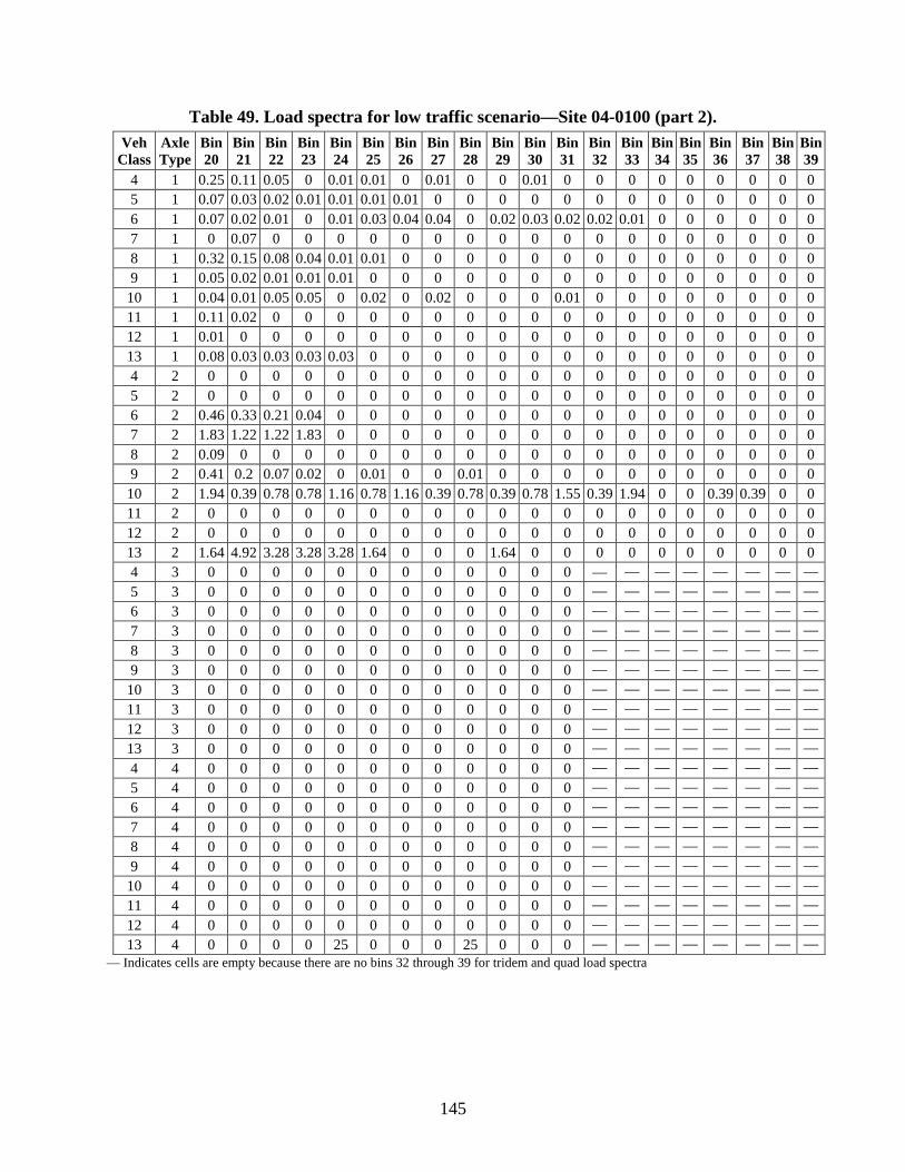
Table 49. Load spectra for low traffic scenario—Site 04-0100 (part 2). Veh

Class Axle Type

Bin 20

Bin 21

Bin 22

Bin 23

Bin 24

Bin 25

Bin 26

Bin 27

Bin 28

Bin 29

Bin 30

Bin 31

Bin 32

Bin 33

Bin 34

Bin 35

Bin 36

Bin 37

Bin 38

Bin 39

4 1 0.25 0.11 0.05 0 0.01 0.01 0 0.01 0 0 0.01 0 0 0 0 0 0 0 0 0 5 1 0.07 0.03 0.02 0.01 0.01 0.01 0.01 0 0 0 0 0 0 0 0 0 0 0 0 0 6 1 0.07 0.02 0.01 0 0.01 0.03 0.04 0.04 0 0.02 0.03 0.02 0.02 0.01 0 0 0 0 0 0 7 1 0 0.07 0 0 0 0 0 0 0 0 0 0 0 0 0 0 0 0 0 0 8 1 0.32 0.15 0.08 0.04 0.01 0.01 0 0 0 0 0 0 0 0 0 0 0 0 0 0 9 1 0.05 0.02 0.01 0.01 0.01 0 0 0 0 0 0 0 0 0 0 0 0 0 0 0

10 1 0.04 0.01 0.05 0.05 0 0.02 0 0.02 0 0 0 0.01 0 0 0 0 0 0 0 0 11 1 0.11 0.02 0 0 0 0 0 0 0 0 0 0 0 0 0 0 0 0 0 0 12 1 0.01 0 0 0 0 0 0 0 0 0 0 0 0 0 0 0 0 0 0 0 13 1 0.08 0.03 0.03 0.03 0.03 0 0 0 0 0 0 0 0 0 0 0 0 0 0 0 4 2 0 0 0 0 0 0 0 0 0 0 0 0 0 0 0 0 0 0 0 0 5 2 0 0 0 0 0 0 0 0 0 0 0 0 0 0 0 0 0 0 0 0 6 2 0.46 0.33 0.21 0.04 0 0 0 0 0 0 0 0 0 0 0 0 0 0 0 0 7 2 1.83 1.22 1.22 1.83 0 0 0 0 0 0 0 0 0 0 0 0 0 0 0 0 8 2 0.09 0 0 0 0 0 0 0 0 0 0 0 0 0 0 0 0 0 0 0 9 2 0.41 0.2 0.07 0.02 0 0.01 0 0 0.01 0 0 0 0 0 0 0 0 0 0 0

10 2 1.94 0.39 0.78 0.78 1.16 0.78 1.16 0.39 0.78 0.39 0.78 1.55 0.39 1.94 0 0 0.39 0.39 0 0 11 2 0 0 0 0 0 0 0 0 0 0 0 0 0 0 0 0 0 0 0 0 12 2 0 0 0 0 0 0 0 0 0 0 0 0 0 0 0 0 0 0 0 0 13 2 1.64 4.92 3.28 3.28 3.28 1.64 0 0 0 1.64 0 0 0 0 0 0 0 0 0 0 4 3 0 0 0 0 0 0 0 0 0 0 0 0 — — — — — — — — 5 3 0 0 0 0 0 0 0 0 0 0 0 0 — — — — — — — — 6 3 0 0 0 0 0 0 0 0 0 0 0 0 — — — — — — — — 7 3 0 0 0 0 0 0 0 0 0 0 0 0 — — — — — — — — 8 3 0 0 0 0 0 0 0 0 0 0 0 0 — — — — — — — — 9 3 0 0 0 0 0 0 0 0 0 0 0 0 — — — — — — — —

10 3 0 0 0 0 0 0 0 0 0 0 0 0 — — — — — — — — 11 3 0 0 0 0 0 0 0 0 0 0 0 0 — — — — — — — — 12 3 0 0 0 0 0 0 0 0 0 0 0 0 — — — — — — — — 13 3 0 0 0 0 0 0 0 0 0 0 0 0 — — — — — — — — 4 4 0 0 0 0 0 0 0 0 0 0 0 0 — — — — — — — — 5 4 0 0 0 0 0 0 0 0 0 0 0 0 — — — — — — — — 6 4 0 0 0 0 0 0 0 0 0 0 0 0 — — — — — — — — 7 4 0 0 0 0 0 0 0 0 0 0 0 0 — — — — — — — — 8 4 0 0 0 0 0 0 0 0 0 0 0 0 — — — — — — — — 9 4 0 0 0 0 0 0 0 0 0 0 0 0 — — — — — — — —

10 4 0 0 0 0 0 0 0 0 0 0 0 0 — — — — — — — — 11 4 0 0 0 0 0 0 0 0 0 0 0 0 — — — — — — — — 12 4 0 0 0 0 0 0 0 0 0 0 0 0 — — — — — — — — 13 4 0 0 0 0 25 0 0 0 25 0 0 0 — — — — — — — —

— Indicates cells are empty because there are no bins 32 through 39 for tridem and quad load spectra

145

REFERENCES

1. National Cooperative Highway Research Program (NCHRP), Mechanistic-Empirical Design of New and Rehabilitated Pavement Structures. Final Report, NCHRP Project 1-37A, National Cooperative Highway Research Program, National Research Council, Washington, DC, 2004.

2. AASHTO, AASHTO Guide for Design of Pavement Structures. American Association of State Highway and Transportation Officials, Washington, DC, 1993.

3. Selezneva, O.I., Ayres, M., Ramachandran A., Shirazi, H., Hajek, J., and Von Quintus, H., Development of New Default Traffic Datasets for the MEPDG Using the SPS Traffic Data Collection Pooled-Fund Study Data. Interim Report (Draft), Project Sponsored by Federal Highway Administration, Internal Communication, Elkridge, MD, July 2010.

147

HRDI-30/11-14(500)ERecycledRecyclable

Verification, Refinement, and Applicability of Long-Term ......Verification, Refinement, and...

Documents

Transcript of Verification, Refinement, and Applicability of Long-Term ......Verification, Refinement, and...