Verification and Controller Synthesis for Timed Automata : the tool KRONOS Stavros Trypakis.

Verification and Controller Synthesisfor Timed Automata :

the tool KRONOS

Stavros Trypakis

Timed AutomataTimed AutomataTimed Systems

Gate

Controller

approach

exit

far near

in

enter

x := 0

Train

x := 0 x > 2

x <= 5

lower

down

up

raise

y := 0y <= 1

y <= 2

y >= 1

y := 0

lower

exit

approachz <= 3

z <= 1

raise

z := 0

z := 0

x >= 1


Gate

Controller

exit

far near

in

enter

x := 0

Train

x := 0 x > 2

x <= 5

lower

down

up

raise

y := 0y <= 1

y <= 2

y >= 1

y := 0

lower

exit

approachz <= 3

z <= 1

raise

z := 0

z := 0

time

approachx >= 1


Gate

Controller

exit

far near

in

enter

x := 0

Train

x := 0 x > 2

x <= 5

lower

down

up

raise

y := 0y <= 1

y <= 2

y >= 1

y := 0

lower

exit

approachz <= 3

z <= 1

raise

z := 0

z := 0

approach

timez <= 3

approachx >= 1


Gate

Controller

exit

far near

in

enter

x := 0

Train

x := 0 x > 2

x <= 5

lower

down

up

raise

y := 0y <= 1

y <= 2

y >= 1

y := 0

lower

exit

approachz <= 3

z <= 1

raise

z := 0

z := 0

approach lower

timez <= 3 y <= 1

approachx >= 1


Gate

Controller

exit

far near

in

enter

x := 0

Train

x := 0 x > 2

x <= 5

lower

down

up

raise

y := 0y <= 1

y <= 2

y >= 1

y := 0

lower

exit

approachz <= 3

z <= 1

raise

z := 0

z := 0

approach lower enter

timex > 2 x <= 5

x = 2.1y = 0.9z = 2.1

approachx >= 1

VerificationVerification

Given a system and a property, verify thatthe system satisfies the property.

Types of Analysis

• Branching-time (execution trees): TCTL.

e.g., “whenever the train is in the crossing, the gate is down”

Properties:

• Linear-time (execution sequences): Timed Büchi Automata.

true>=1

task1

task2

Controller SynthesisController Synthesis

Given a controller embedded in a certain environment,and a property, restrict the controller so that the propertyis satisfied, no matter how the environment behaves.

Properties:

• Invariance: the controller keeps the system inside a set of safe states.

• Reachability: the controller leads the system to a set of target states.

Types of Analysis

Synthesizing a ControllerSynthesizing a Controller

Timed Systems

Gate

Controller

Train

lower

down

up

raise

y := 0y <= 1

y <= 2

y >= 1

y := 0

lower

exit

approach

raise

approach

exit

far near

in

enter

x := 0

x := 0 x > 2

x <= 5

x <= 1

x <= 0

Environment

x >= 1

MotivationsMotivationsMotivations

Enumerative:region by

region

Symbolic:unions ofregions

encoded bypolyhedra

Reachability TBA

Region graph

Kronosforward

Kronosbackward(fix-point)

ControllerSynthesisModel checking

Too big: 10 for TGC4


TCTL

• No diagnostics• Expensive: - complementation - nested fix-points

non-convexpolyhedra

ContributionsContributionsContributions

Region graph

Kronosforward


Time-abstracting Bisimulation(Quotient graph)

On-the-flyverification



Re-useuntimed

resources(algorithms

+ tools)

Generate & Verify

at the same time

Reachability TBA ControllerSynthesisModel checking

TCTL

Enumerative:region by

region

Symbolic:unions ofregions

encoded bypolyhedra

PlanPlan

• Analysis with the Time-abstracting Bisimulation

• On-the-fly Verification

• Diagnostics

• Controller Synthesis

• Case studies

• Conclusions and Perspectives

• Implementation

The Time-abstracting BisimulationThe Time-abstracting Bisimulation

Equivalence on TA states:

Preserve discretestate changes.

Abstract exacttime delays.

s1 s2

s3

a

s4a 1

s1 s2

s3

Analysis with Time-abstracting Bisimulations

2

s41, 2 R

The Time-abstracting Quotient GraphThe Time-abstracting Quotient Graph

- Nodes = symbolic states (equivalence classes).- Edges = symbolic transitions (discrete and time).

• Finite symbolic graph:

• Basic property: pre-stability

Q1 Q2

s1 s2

a

Q1 Q2

s1 s2a

Q1 pre (Q2) = Q1a

Q1 pre (Q2) = Q1time


• The quotient induced by the greatest time-abstracting bisimulation defined on the TA.

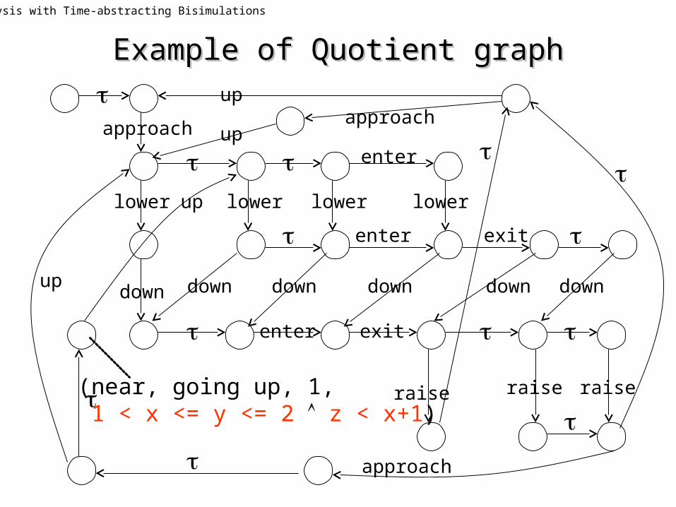
Example of Quotient graphExample of Quotient graph


down

lower

up

exit

raise

enter

approach

approach

approach

up

up

up down down down down down

lower lowerlower

raise raise

exitenter

enter

(near, going up, 1, 1 < x <= y <= 2 z < x+1)

Verification on the Quotient graph:Verification on the Quotient graph:Linear-timeLinear-time


Every cycle in the quotient graph contains an infinite runand vice versa.

Q1 Q4Q3Q2

s1 s2 s3 s4s5 ...

Timed Büchi Automatamodel checking

DFS for cycles or SCCsin the quotient graph

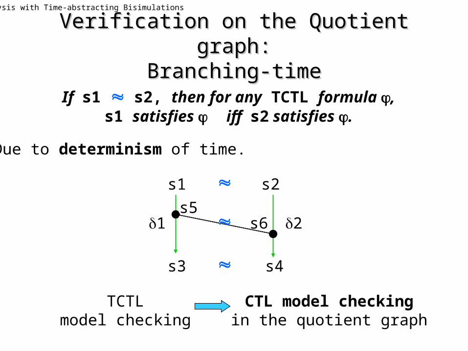
Verification on the Quotient graph:Verification on the Quotient graph:Branching-timeBranching-time


If s1 s2, then for any TCTL formula ,s1 satisfies iff s2 satisfies .

TCTLmodel checking

CTL model checkingin the quotient graph

1

s1 s2

s3

2

s4

s5s6

Due to determinism of time.

PlanPlan



• Diagnostics


• Case studies


• Implementation

The Simulation GraphThe Simulation Graph

- Start from an initial node (symbolic state).

- Add successor nodes using post( ) operator.

• Finite symbolic graph generated dynamically by forward reachability :

• Basic property: post-stability

a

Q1 Q2

s1

s2

a

Q2 = post (post (Q1))time a

On-The-Fly Verification

- Stop when a node is already visited.


Idea of proof: every post-stable cycle can be pre-stabilized

Q1 Q2 Q3Q0

Q3 pre(Q1)

Verification on the Simulation graph:Verification on the Simulation graph:Linear-timeLinear-time

Every cycle in the simulation graph contains an infinite runand vice versa.


Q1 Q2 Q3Q0

Verification on the Simulation graph:Verification on the Simulation graph:Linear-timeLinear-time

Every cycle in the simulation graph contains an infinite runand vice versa.

The process terminates, yielding a non-empty, pre-stable cycle

can use pre-stability to extract an infinite run.

Timed Büchi Automatamodel checking

DFS for cycles or SCCsin the simulation graph


Verification on the Simulation graph:Verification on the Simulation graph:Branching-timeBranching-time

TCTLmodel checking

• Branching-time properties not preserved: no pre-stability.

• But :Nested problems

of Timed Büchi Automata model checking

Abstractions for on-the-fly verification

• Clock activity : eliminate inactive clocks polyhedra change dimension dynamically

• Closure (or widening) : extrapolate bounds when they go beyond some maximal threshold

• Inclusion, convex hull, etc.

PlanPlan



• Diagnostics


• Case studies


• Implementation

Timed DiagnosticsTimed Diagnostics

Diagnostics

Symbolic diagnostics not sufficient: no information on delays.

• Finite diagnostics: extract runs from symbolic paths.

Need timed diagnostics, e.g.:

s3+

a

s1 s2ac

s4cb

s3b

approach lower enter2.5 1 ...

choose points and delays in polyhedra(matrix representation)

e.g., in quotient graph:

Q1 Q3Q2 Q4 Q5

Timed DiagnosticsTimed Diagnostics

Diagnostics

Symbolic diagnostics not sufficient: no information on delays.

• Infinite diagnostics: this method does not terminate.

Need timed diagnostics, e.g.:

approach lower enter2.5 1 ...

...

- a periodic run does not always exist- … unless if no strict constraints (<, >) in symbolic cycle

PlanPlan



• Diagnostics


• Case studies


• Implementation

Controller SynthesisController SynthesisController Synthesis

• Untimed case:

- Model: graph with edges labeled controllable - uncontrollable.

...- Semantics: strategy = sub-graph containing, for each node, at least one controllable

and all uncontrollable successors

...

c uuc c

• Timed case:

- Model: TA with discrete actions labeled controllable - uncontrollable

- Semantics: dense strategies (time transitions ?)

u

sc

s

Controller Synthesis using Fix-pointsController Synthesis using Fix-points

Controller Synthesis

• controllable-predecessor operator contr-pre(Q) = all states from which the system can be led to Q, no matter how the environment behaves.

• compute winning states as fix-points of contr-pre( ).

• obtain controller = intersect TA with winning states.

Q

c

us

• method costly (complementation in contr-pre( ), fix-point computes maximal strategy).

On-the-fly Controller SynthesisOn-the-fly Controller Synthesis


• on-the-fly algorithm for the untimed case: - a DFS is used to find a strategy - the algorithm stops as soon as first strategy is found

• untimed algorithm can be used for timed synthesis, too:

TA Quotientgraph

untimedalgorithm (symbolic)

strategycontroller

pre-stability of quotient graph essential for correctness cannot use simulation graph…

On-the-fly synthesis in quotient graphOn-the-fly synthesis in quotient graph


down

lower

up

exit

raise

enter

approachapproach

approach

up

up

up down down down down down

lower lowerlower

raise raise

exitenter

enter

PlanPlan



• Diagnostics


• Case studies


• Implementation

Implementation in KronosImplementation in Kronos

Implementation

Full TCTLmodel

checking

Minim.TBA

model checking

ControllerSynthesis

(On-the-fly) ParallelComposition

Reachability

Aldebaran:- reduction/comparison- model checking- simulation/visualization

Safe TCTLmodel

checking

TA ...TA TA

TA

TBA

initialpartition

QuotientGraph

P,<=k P, ... PP, P

Yes/No,diagnostics

Restricted TA(controller)

Yes/No,diagnostics

Matrix library

Connection of Kronos to Open-CaesarConnection of Kronos to Open-Caesar

Implementation

Optimizedpolyhedra library

Open-Caesar’sgraph library

Kronos-Open

input: model

TA network+ discrete shared vars.+ message passing

model.c

C-compiler

code generationinterface to

Open-Caesar

evaluator

generator

exhibitor

simulator

profounder

-calculus formula

regular expression

State formulaTBA

Yes/No + untimed diagnostics

- Reachability + timed diagnostics- TBA model checking.

Yes/No + untimed diagnostics

Simulation graph

PlanPlan



• Diagnostics


• Case studies


• Implementation

Case StudiesCase Studies

• FRP/DT protocol (project with CNET, Lannion) - found inconsistency error (known to designers)

• Bang&Olufsen protocol (from previous case study by Uppaal) - found error not reported in Uppaal case study

• Multimedia documents (from INRIA project OPERA) - modeled documents as Timed Automata - checked executability (model checking) - computed schedulers (controller synthesis)

Case studies

• Benchmarks: STARI chip, Fischer’s protocol, CSMA/CD protocol, FDDI protocol, Philips protocol

Experiences: performanceExperiences: performance

• improved performance in benchmarks, often by many orders of magnitude.

Case studies

• tools and techniques able to handle real-world case studies:

7- Bang&Olufsen: 30 discrete variables, large constants simulation graph = 10 symbolic states, 15 mins, 300 MB counter example = 1500 steps long, 20 secs

- STARI: 30 clocks, 60 boolean variables

• often bottleneck is discrete state space

Experiences: comparison of methodsExperiences: comparison of methodsCase studies

Techniques are complementary

Quotient graph Simulation graph

Fischer

Real-timescheduling

Philips

CSMA/CD

nodes edges time(secs)

22,085

929

481

503

1,503

875

122,804

1,001

70

1

3

1,000

nodes edges time(secs)

164,935

10,839

60

194

22,382

96

457,799

488

150

1

1

1,060

Casestudy

ConclusionsConclusions

Practicality not measured only in seconds, megabytes

Conclusions

• Expressive models : - discrete variables (Kronos-open) - different property-specification formalisms (TBA, TCTL)

• Variety : - of problems (model checking, controller synthesis) - of techniques (on-the-fly, using untimed tools) - of feedback (symbolic/timed diagnostics, controllers)

• Case studies : source of inspiration.

PerspectivesPerspectives

• Performance: - homogeneous representation of discrete and continuous state space (e.g., BDDs + polyhedra) - adaptation/combination with untimed techniques reducing interleavings (e.g., partial orders)

Perspectives

• Methodology for correct & efficient modeling: - domain-specific guidelines - composition theory

• Controller synthesis: - more properties (e.g., liveness) - more efficient techniques (e.g., completely on-the-fly)

Verification and Controller Synthesis for Timed Automata : the tool KRONOS Stavros Trypakis.

Documents

Transcript of Verification and Controller Synthesis for Timed Automata : the tool KRONOS Stavros Trypakis.