VERA Training: 3D Assemblies

VERA Training – Core SimulatorFebruary 13, 2019

VERA Users Group MeetingOak Ridge National Laboratory

2

Training Objectives

Learn how to:• Set up 3D Problems• Set axial mesh• Add grids, nozzles, core plates, etc.• Set number of cores• Add T/H Feedback with CTF• Run Multiple Statepoints

3

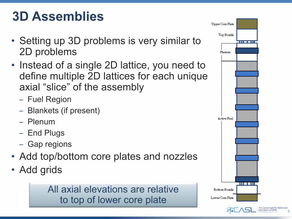
3D Assemblies

• Setting up 3D problems is very similar to 2D problems

• Instead of a single 2D lattice, you need to define multiple 2D lattices for each unique axial “slice” of the assembly– Fuel Region– Blankets (if present)– Plenum– End Plugs– Gap regions

• Add top/bottom core plates and nozzles• Add grids

All axial elevations are relative to top of lower core plate

4

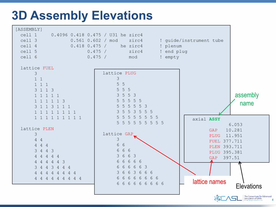
3D Assembly Elevations[ASSEMBLY]

cell 1 0.4096 0.418 0.475 / U31 he zirc4cell 3 0.561 0.602 / mod zirc4 ! guide/instrument tubecell 4 0.418 0.475 / he zirc4 ! plenumcell 5 0.475 / zirc4 ! end plugcell 6 0.475 / mod ! empty

lattice FUEL31 11 1 13 1 1 31 1 1 1 11 1 1 1 1 33 1 1 3 1 1 11 1 1 1 1 1 1 11 1 1 1 1 1 1 1 1

lattice PLEN34 44 4 43 4 4 34 4 4 4 44 4 4 4 4 33 4 4 3 4 4 44 4 4 4 4 4 4 44 4 4 4 4 4 4 4 4

lattice PLUG35 55 5 53 5 5 35 5 5 5 55 5 5 5 5 33 5 5 3 5 5 55 5 5 5 5 5 5 55 5 5 5 5 5 5 5 5

lattice GAP36 66 6 63 6 6 36 6 6 6 66 6 6 6 6 33 6 6 3 6 6 66 6 6 6 6 6 6 66 6 6 6 6 6 6 6 6

axial ASSY6.053

GAP 10.281PLUG 11.951FUEL 377.711PLEN 393.711PLUG 395.381GAP 397.51

assembly name

lattice names Elevations

5

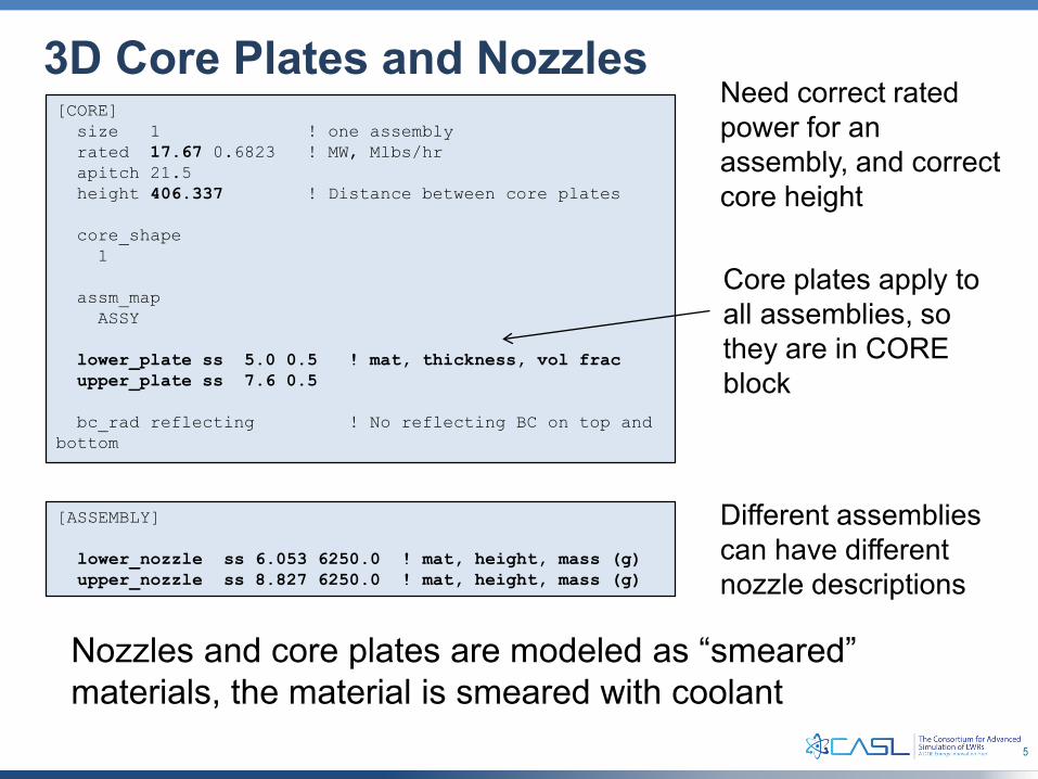
3D Core Plates and Nozzles[CORE]

size 1 ! one assemblyrated 17.67 0.6823 ! MW, Mlbs/hrapitch 21.5height 406.337 ! Distance between core plates

core_shape1

assm_mapASSY

lower_plate ss 5.0 0.5 ! mat, thickness, vol fracupper_plate ss 7.6 0.5

bc_rad reflecting ! No reflecting BC on top and bottom

[ASSEMBLY]

lower_nozzle ss 6.053 6250.0 ! mat, height, mass (g)upper_nozzle ss 8.827 6250.0 ! mat, height, mass (g)

Core plates apply to all assemblies, so they are in CORE block

Different assemblies can have different nozzle descriptions

Nozzles and core plates are modeled as “smeared” materials, the material is smeared with coolant

Need correct rated power for an assembly, and correct core height

6

3D Assembly Grids

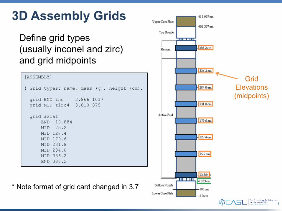
[ASSEMBLY]

! Grid types: name, mass (g), height (cm),

grid END inc 3.866 1017grid MID zirc4 3.810 875

grid_axialEND 13.884MID 75.2MID 127.4MID 179.6MID 231.8MID 284.0MID 336.2END 388.2

Define grid types(usually inconel and zirc)and grid midpoints

Grid Elevations(midpoints)

* Note format of grid card changed in 3.7

7

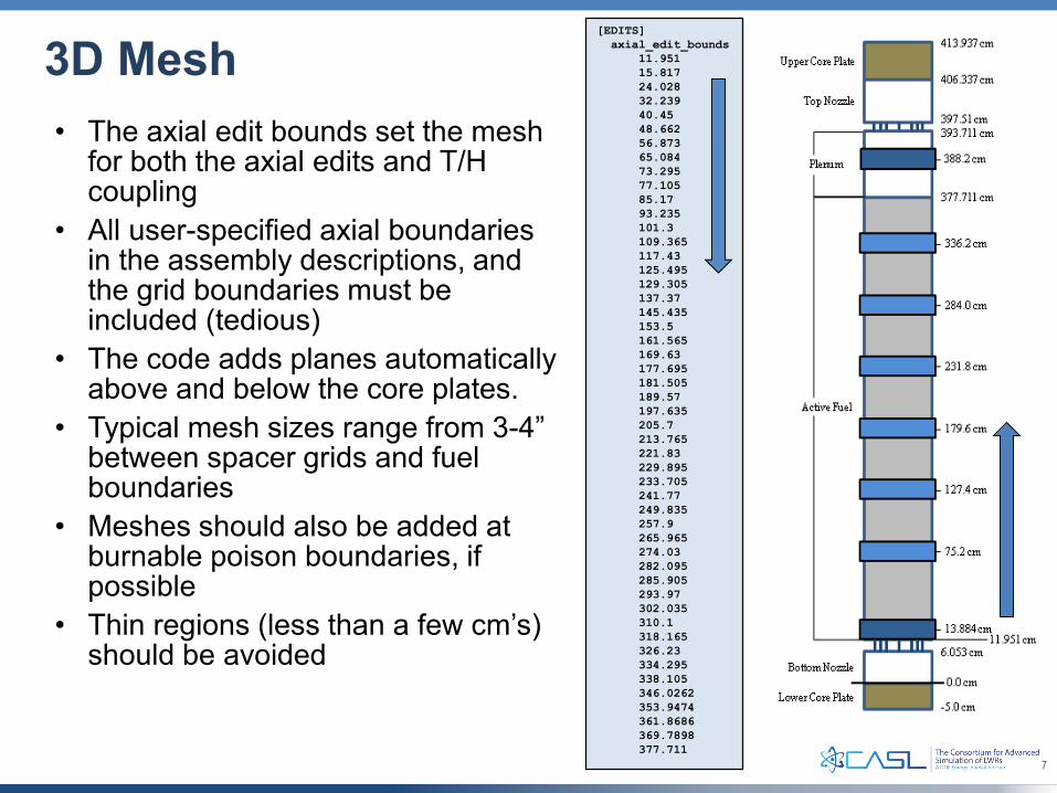
[EDITS]axial_edit_bounds

11.95115.81724.02832.23940.4548.66256.87365.08473.29577.10585.1793.235101.3109.365117.43125.495129.305137.37145.435153.5161.565169.63177.695181.505189.57197.635205.7213.765221.83229.895233.705241.77249.835257.9265.965274.03282.095285.905293.97302.035310.1318.165326.23334.295338.105346.0262353.9474361.8686369.7898377.711

3D Mesh• The axial edit bounds set the mesh

for both the axial edits and T/H coupling

• All user-specified axial boundaries in the assembly descriptions, and the grid boundaries must be included (tedious)

• The code adds planes automatically above and below the core plates.

• Typical mesh sizes range from 3-4” between spacer grids and fuel boundaries

• Meshes should also be added at burnable poison boundaries, if possible

• Thin regions (less than a few cm’s) should be avoided

8

Parallel Decomposition

• Domain decomposition can be used to split problem up into axial and radial parallel regions

• Total number of CPU cores = axial regions x radial regions

• Radial decomposition will be described in full-core section

• Axial decomposition is done by plane• With N planes, you can assign from 1 to N CPU cores

to problem

9

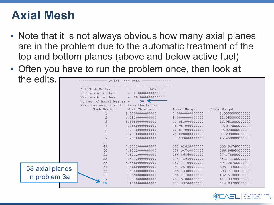
Axial Mesh• Note that it is not always obvious how many axial planes

are in the problem due to the automatic treatment of the top and bottom planes (above and below active fuel)

• Often you have to run the problem once, then look at the edits. ============== Axial Mesh Data ==============

=============================================AutoMesh Method = NONFUELMinimum Axial Mesh = 2.0000000000000Maximum Axial Mesh = 20.000000000000Number of Axial Meshes = 58Mesh regions, starting from the bottom:

Mesh Region Mesh Thickness Lower Height Upper Height1 5.0000000000000 0.0000000000000 5.00000000000002 6.0530000000000 5.0000000000000 11.0530000000003 5.8980000000000 11.053000000000 16.9510000000004 3.8660000000000 16.951000000000 20.8170000000005 8.2110000000000 20.817000000000 29.0280000000006 8.2110000000000 29.028000000000 37.2390000000007 8.2110000000000 37.239000000000 45.450000000000……49 7.9212000000000 351.02620000000 358.9474000000050 7.9212000000000 358.94740000000 366.8686000000051 7.9212000000000 366.86860000000 374.7898000000052 7.9212000000000 374.78980000000 382.7110000000053 8.5560000000000 382.71100000000 391.2670000000054 3.8660000000000 391.26700000000 395.1330000000055 3.5780000000000 395.13300000000 398.7110000000056 3.7990000000000 398.71100000000 402.5100000000057 8.8270000000000 402.51000000000 411.3370000000058 7.6000000000000 411.33700000000 418.93700000000

58 axial planes in problem 3a

10

Load Balance

• To get the best performance, you should try to balance the computational load as evenly as possible

• Set the problem up so each core has same “load”, i.e. same number of axial planes

• For fastest run-time, use one plane per core• For less CPU usage, use two or three planes per core• Example – 58 axial planes

– With 58 cores, there is one plane per core– With 29 cores, there is two planes per core– Using something in between (like 35) will not be any faster because

some cores will have 1 plane and some cores will have 2 planes.– Run-time is dictated by the “slowest” core.

11

Setting Number of Nodes with PBS• Computer nodes have multiple cores• You can only request jobs with integer multiples of “nodes”

– Lemhi has 40 cores/node (ppn – processors per node)– Other computers might have 12 or 24 or 32

• To find number of “nodes”, divide total number of cores needed by cores/node, then round up

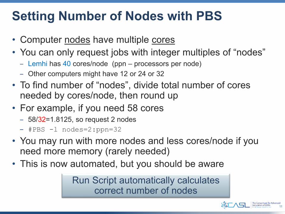
• For example, if you need 58 cores– 58/32=1.8125, so request 2 nodes– #PBS -l nodes=2:ppn=32

• You may run with more nodes and less cores/node if you need more memory (rarely needed)

• This is now automated, but you should be aware

Run Script automatically calculates correct number of nodes

12

Set Number of Cores

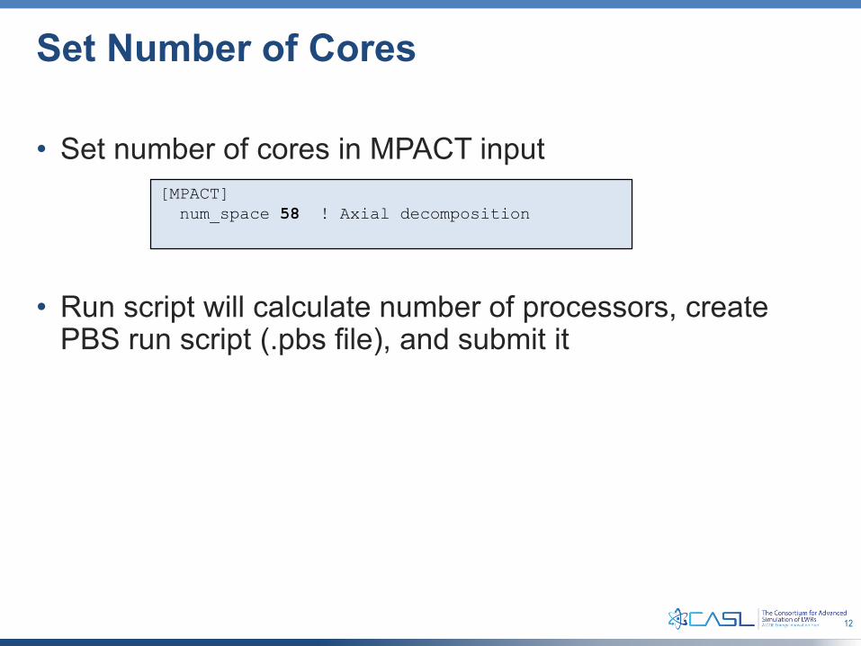
• Set number of cores in MPACT input

• Run script will calculate number of processors, create PBS run script (.pbs file), and submit it

[MPACT]num_space 58 ! Axial decomposition

13

Class Exercise 5: Run 3D Problem

• The 3D sample problem is “3a.inp”cp $VERAHOME/share/VERAIn/Progression_Problems/3a.inp .

• The 3D Problems take longer to run, so you should use more cores and space decomposition than the 2D problem

• If possible, a good solution is to run one axial plane per core (or two planes per core)

• The sample input has 58 cores, but this can be changed

Copy Sample Input and Run

14

3D Questions for Discussion

• How do you add IFBA to 3D Problems?– You may need different axial zones for IFBA and/or blankets

• How do you add WABA to 3D Problems?– Need to add different axial zones in the INSERT block for WABA

and/or blankets– Make sure the elevations in the INSERT block match the

ASSEMBLY block– Add WABA axial boundaries to EDIT regions

• How do you deplete in 3D?– Same way as 2D

15

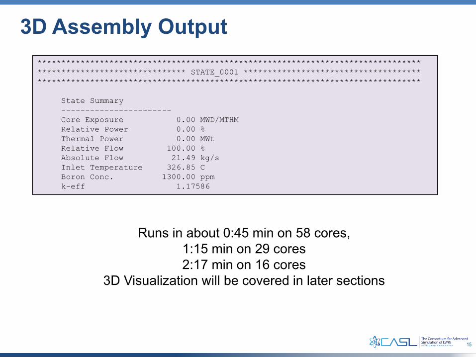
3D Assembly Output*************************************************************************************************************** STATE_0001 *********************************************************************************************************************

State Summary-----------------------Core Exposure 0.00 MWD/MTHMRelative Power 0.00 %Thermal Power 0.00 MWtRelative Flow 100.00 %Absolute Flow 21.49 kg/sInlet Temperature 326.85 CBoron Conc. 1300.00 ppmk-eff 1.17586

Runs in about 0:45 min on 58 cores, 1:15 min on 29 cores2:17 min on 16 cores

3D Visualization will be covered in later sections

16

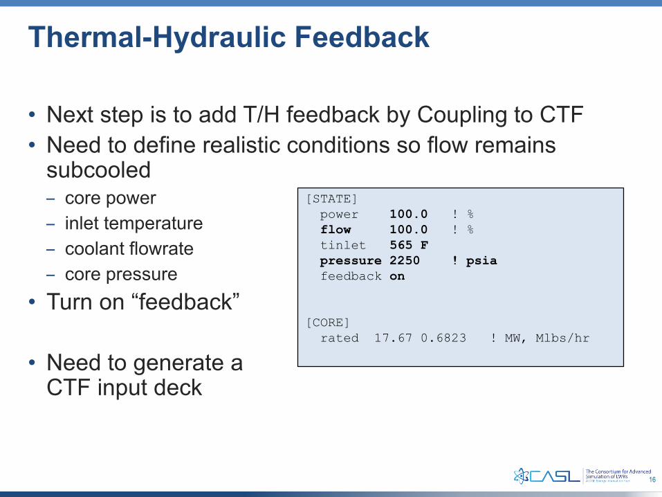
Thermal-Hydraulic Feedback

• Next step is to add T/H feedback by Coupling to CTF• Need to define realistic conditions so flow remains

subcooled– core power – inlet temperature – coolant flowrate– core pressure

• Turn on “feedback”

• Need to generate a CTF input deck

[STATE]power 100.0 ! %flow 100.0 ! %tinlet 565 Fpressure 2250 ! psiafeedback on

[CORE]rated 17.67 0.6823 ! MW, Mlbs/hr

17

Generate CTF Input Deck

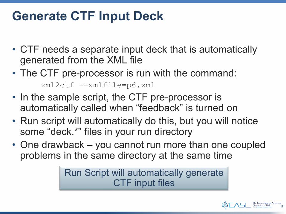
• CTF needs a separate input deck that is automatically generated from the XML file

• The CTF pre-processor is run with the command:xml2ctf --xmlfile=p6.xml

• In the sample script, the CTF pre-processor is automatically called when “feedback” is turned on

• Run script will automatically do this, but you will notice some “deck.*” files in your run directory

• One drawback – you cannot run more than one coupled problems in the same directory at the same time

Run Script will automatically generate CTF input files

18

Parallel CTF

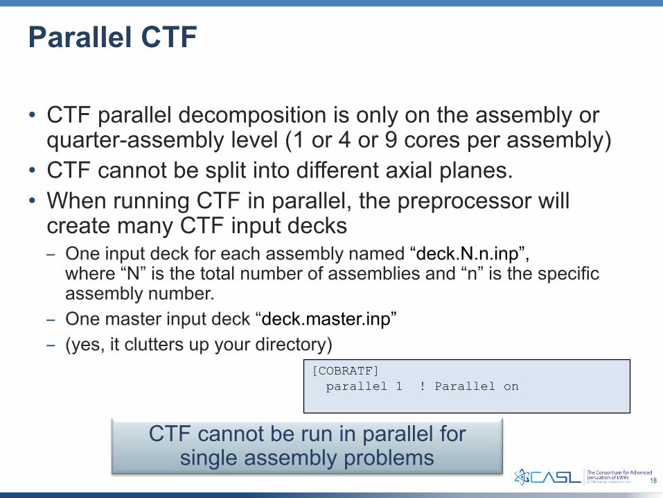
• CTF parallel decomposition is only on the assembly or quarter-assembly level (1 or 4 or 9 cores per assembly)

• CTF cannot be split into different axial planes.• When running CTF in parallel, the preprocessor will

create many CTF input decks– One input deck for each assembly named “deck.N.n.inp”,

where “N” is the total number of assemblies and “n” is the specific assembly number.

– One master input deck “deck.master.inp”– (yes, it clutters up your directory)

CTF cannot be run in parallel for single assembly problems

[COBRATF]parallel 1 ! Parallel on

19

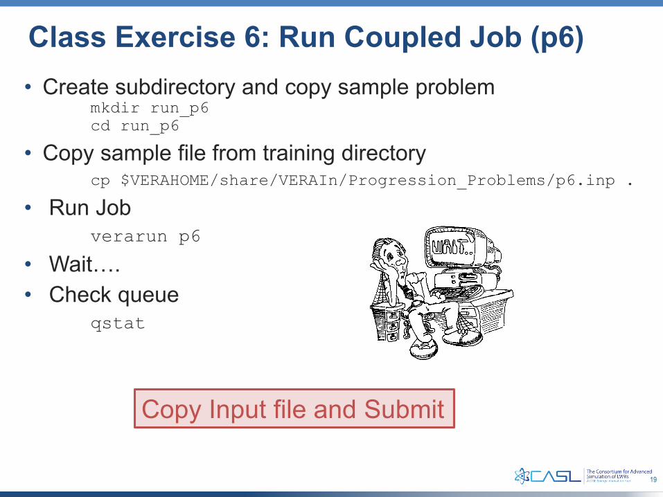
Class Exercise 6: Run Coupled Job (p6)• Create subdirectory and copy sample problem

mkdir run_p6cd run_p6

• Copy sample file from training directorycp $VERAHOME/share/VERAIn/Progression_Problems/p6.inp .

• Run Jobverarun p6

• Wait….• Check queue

qstat

Copy Input file and Submit

20

3D Coupled Problem Output

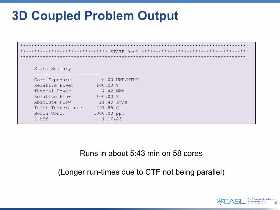
*************************************************************************************************************** STATE_0001 *********************************************************************************************************************

State Summary-----------------------Core Exposure 0.00 MWD/MTHMRelative Power 100.00 %Thermal Power 4.42 MWtRelative Flow 100.00 %Absolute Flow 21.49 kg/sInlet Temperature 291.85 CBoron Conc. 1300.00 ppmk-eff 1.16483

Runs in about 5:43 min on 58 cores

(Longer run-times due to CTF not being parallel)

21

Submit other jobs if time permits…

• Submit IFBA or WABA jobs

• Submit 3D depletion jobs

22

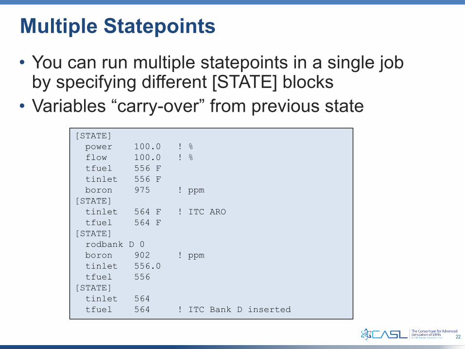
Multiple Statepoints• You can run multiple statepoints in a single job

by specifying different [STATE] blocks• Variables “carry-over” from previous state

[STATE]power 100.0 ! %flow 100.0 ! %tfuel 556 Ftinlet 556 Fboron 975 ! ppm

[STATE]tinlet 564 F ! ITC AROtfuel 564 F

[STATE]rodbank D 0boron 902 ! ppmtinlet 556.0tfuel 556

[STATE]tinlet 564tfuel 564 ! ITC Bank D inserted

23

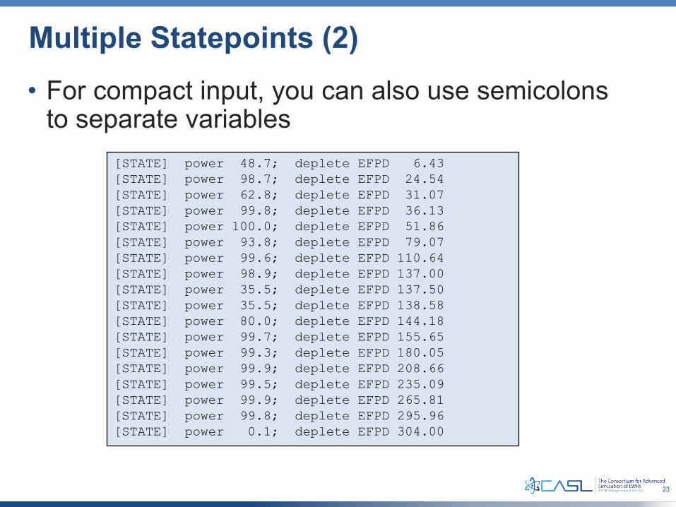
Multiple Statepoints (2)• For compact input, you can also use semicolons

to separate variables[STATE] power 48.7; deplete EFPD 6.43[STATE] power 98.7; deplete EFPD 24.54[STATE] power 62.8; deplete EFPD 31.07[STATE] power 99.8; deplete EFPD 36.13[STATE] power 100.0; deplete EFPD 51.86[STATE] power 93.8; deplete EFPD 79.07[STATE] power 99.6; deplete EFPD 110.64[STATE] power 98.9; deplete EFPD 137.00[STATE] power 35.5; deplete EFPD 137.50[STATE] power 35.5; deplete EFPD 138.58[STATE] power 80.0; deplete EFPD 144.18[STATE] power 99.7; deplete EFPD 155.65[STATE] power 99.3; deplete EFPD 180.05[STATE] power 99.9; deplete EFPD 208.66[STATE] power 99.5; deplete EFPD 235.09[STATE] power 99.9; deplete EFPD 265.81[STATE] power 99.8; deplete EFPD 295.96[STATE] power 0.1; deplete EFPD 304.00

24

Questions?

www.casl.gov