VENTURE EVALUATION AND REVIEW TECHNIQUE (VERT) … · 2015-06-25 · 1-2 VERT History 2 2 The VERT...

fih* DVf* boo

RIA-79-U647

VENTURE EVALUATION

AND

REVIEW TECHNIQUE

(VERT) TECHNICAL k LIBRARY

NOVEMBER 1979

DECISION MODELS DIRECTORATE

US ARMY ARMAMENT MATERIEL READINESS COMMAND

ROCK ISLAND, ILLINOIS 61299

SECURITY CLASSIFICATION OF THIS PAGE (Wh»n Data Entered)

REPORT DOCUMENTATION PAGE READ INSTRUCTIONS BEFORE COMPLETING FORM

1. REPORT NUMBER

DRSAR-DM-T905 2. GOVT ACCESSION NO. 3. RECIPIENT'S CATALOG NUMBER

4. TITLE Cand Subtitle.)

Users'/Analysts' Manual for the Venture Evaluation and Review Technique

5. TYPE OF REPORT & PERIOD COVERED

Final Report - Indefinite

6. PERFORMING ORG. REPORT NUMBER

7. AUTHORf*.)

G. L. Moeller B. CONTRACT OR GRANT NUMBERfa.)

9. PERFORMING ORGANIZATION NAME AND ADDRESS

Decision Models Directorate Rock Island, IL 61299

10. PROGRAM ELEMENT, PROJECT, TASK AREA ft WORK UNIT NUMBERS

11. CONTROLLING OFFICE NAME AND ADDRESS

Decision Models Directorate Rock Island, IL 61299

12. REPORT DATE

November 1979 13- NUMBER OF PAGES

14. MONITORING AGENCY NAME ft AODRESSCI/dl//ersn( from Controlling Of/ice) 15. SECURITY CLASS, (ol thla report)

Unclassified 15«. DECLASSIFICATION/DOWN GRADING

SCHEDULE

16. DISTRIBUTION STATEMENT (ot thla Report)

Approved for public release, distribution unlimited

17. DISTRIBUTION STATEMENT (ol the abstract entered In Block 20, It different from Report)

IB. SUPPLEMENTARY NOTES

Point of Contact: Mr. Albert J. Patsche, AUTOVON 793-5292,

19- KEY WORDS fContinue on reverse aide if necessary and identify by block number)

Risk Analysis Schedule Risk Performance Risk Capital Requirements

Networks Computer Program

20. ABSTRACT (Continue on reverse altte If necessary and Identify by block number)

This report is a User's/Analysts' Manual for the Venture Evaluation and Review Technique (VERT). The basic purpose of VERT is to support management in the assessment and quantification of the risk involved in new ventures and projects, to provide estimates of capital requirements, and to evaluate on- going projects, programs, and systems. VERT is totally computerized. It permits analyses of risk in three parameters — time, cost, and performance. More importantly, it permits the user to scope his problem in any level of detail desired.

DD ) JAN 73 1473 EDITION OF t NOV 6S IS OBSOLETE

SECURITY CLASSIFICATION OF THIS PAGE (When Data Entered)

SECURITY CLASSIFICATION OF THIS PACEfffhan Dmlm Bntmrmd)

*? ;.•

SECURITY CLASSIFICATION OF THIS PAGEfWien Data Entered)

ABSTRACT

This Users'/Analysts' Manual provides information in sufficient detail wrSSnSiJ CcDTllat„?nT

and aPPlication 0^ the VENTURE EVALUATION AND REVIEW TECHNIQUE (VERT). VERT is a computerized, mathematical oriented simulation network technique designed to model decision environments under risk His- torically. VERT has been used principally to assess the risks involved in the undertaking of a new venture, as well as in the estimation of future capital requirements, control monitoring, and overall evaluation of on-qoinq projects, programs, and systems. Modeling is accomplished with a small set of easily comprehended operators which readily facilitates the structuring of a symbolic pictorial network layout of the system under study. VERT is an adaptive tool, thereby allowing the scope and level of abstraction to rest a most entirely in the hands of the analyst. Thus, modeling can be accomplished on a one-for-one basis, whereby one real world event and activ- lly ^correspondingly represented symbolically as one event and activity in the VERT network; or, modeling can also be accomplished on a compressive basis whereby a multitude of real world events and activities are compressed into the symbolic representation of a few events and activities in the VERT network.

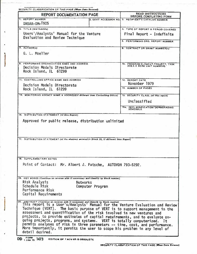
FOREWORD

This report provides a description and instructions in sufficient detail to permit installation and use of the Venture Evaluation and Review Technique (VERT). The technique and this documentation were developed by the Joint Conventional Ammunition Program Coordinating Group Decision Models Directorate. This directorate is now the Decision Models Directorate of the US Army Armament Materiel Readiness Command.

Configuration management of VERT will be retained by the Decision Models Directorate. Proposals for modification and inquiries with respect to application should be addressed to the Commander, US Army Armament Materiel Readiness Command, ATTN: DRSAR-DM, Rock Island, IL 61299. Telephone inquiries should be addressed to Mr. Albert J. Patsche, AUTOVON 793-5292.

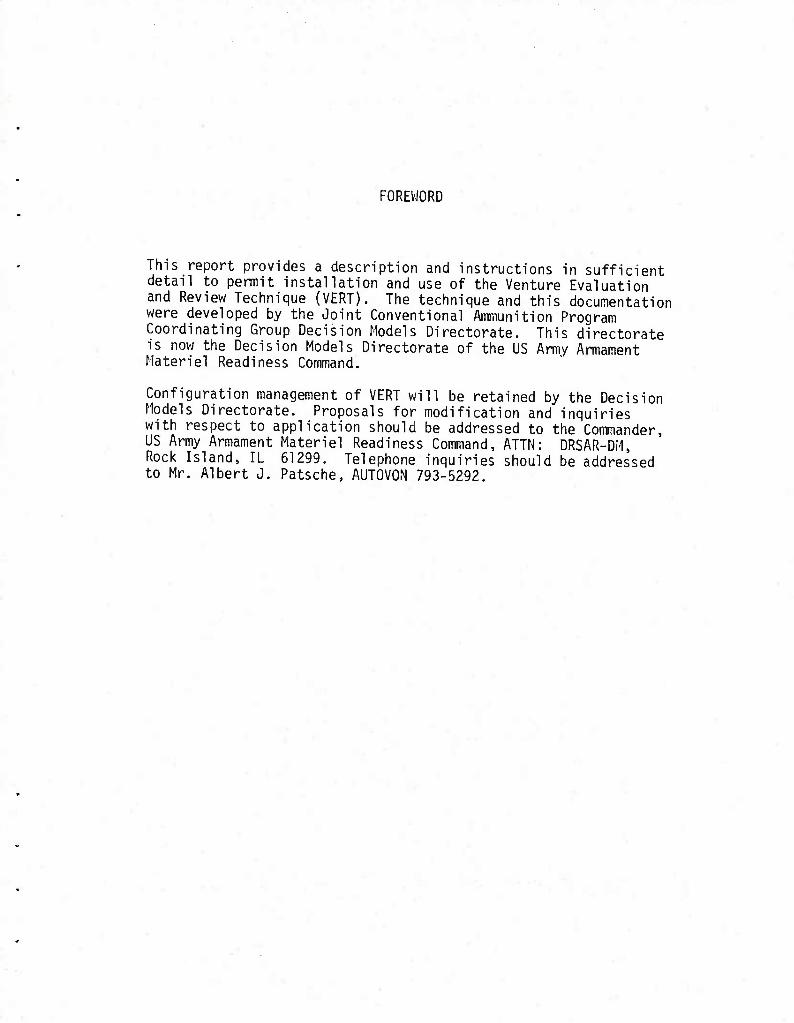
TABLE OF CONTENTS

CHAPTER Page

1 Introduction ] 1-1 Management Overview of VERT 1 1-2 VERT History 2

2 The VERT System 5 2-1 Description of the VERT Process 5 2-2 Operands 8

3 Input for the Computer Program 16 3-1 Overview 16 3-2 Layouts -16

A Control and Problem Option Cards 16 Al Control Card 16 A2 Problem Identification Option Card 21 A3 Full Print Trip Option Card 21 A4 Correlation Computation and Plot Option Card 22 A5 Cost-Performance Time Intervals Option Card(s) 22 A6 Composite Terminal Node Minimums and Maximums

Option Card 24

B Master Arc Card and Accompanying Satellite Arc Cards 24 Bl Master Arc Card 24 B2 Time Statistical Distribution Satellite Arc Card 25 B3 Cost Statistical Distribution Satellite Arc Card 27 B4 Performance Statistical Distribution Satellite Arc Card 27 B5 Time Histogram Satellite Arc Card(s) 27 B6 Cost Histogram Satellite Arc Card(s) 28 B7 Performance Histogram Satellite Arc Card(s) 28 B8 Time Mathematically Related Satellite Arc Card(s) 28 B9 Cost Mathematically Related Satellite Arc Card(s) 32 BIO Performance Mathematically Related Satellite Arc Card(s) 33 Bll Filter Number 1 Satellite Arc Card 34 B12 Filter Number 2 Satellite Arc Card 35 B13 Filter Number 3 Satellite Arc Card 35 B14 Monte Carlo Satellite Arc Card 36 B15 Monte Carlo Time Conditioned Satellite Arc Card 37 B16 Monte Carlo Cost Conditioned Satellite Arc Card 37 B17 Monte Carlo Performance Conditioned Satellite Arc Card 37 B18 Slack Histogram Satellite Arc Card 38

C End of Arc Data Signaler 38

D Master Node Card and Accompanying Satellite Node Cards 38 Dl Master Node Card 38 D2 Histogram Satellite Node Card 41 D3 Subtract Satellite Node Card 42 D4 Slack Histogram Satellite Node Card 42

E End of Node Data Signaler 43

4 Error and Warning Messages 44

5 Example Problem - Future Electric Power Generating Methods 59

6 Auxiliary Program Used to Aid VERT 85 6-1 DIMEN the Core Storage Dimensioning Program 85

A Definition of Inputs 85

B Example Output 85

H

CHAPTER 1 INTRODUCTION

1-1. Management Overview of VERT

One of the most pervasive and recurring situations encountered by management Is the requ rementto make decisions with incomplete or Inadequate Information about the alternatives. These DECISIONS UNDER RISK usually relate to the th?ee

on^nvesSreL?) "^ SChedUle ^ performance (Production levels, returns

To assist the manager in making decisions under risk, many techniques have been developed and used over the past years. Linear programming, game theory and various mode mg techniques are some examples. One of the most popular modeling approaches in recent years for modeling complex problems has been the technique called SIMULATION. The easy accessibility to large scale general purpose computers has made this technique a valuable tool for the manager.

• V5RT, !H ic™nW for VENTURE EVALUATION AND REVIEW TECHNIQUE, is a computerized, mathematical oriented simulation networking technique designed to svs- tematically assess the risks involved in the undertaking of a new venture and in the resource planning, control monitoring and overall evaluation of on-qoinq projects, programs and systems. The features structured in VERT enable expedi- tious modeling of extremely complex decisions which heretofore had defied analysis. Modeling is accomplished with a small set of easily comprehensible operators which readily facilitates the structuring of a symbolic pictorial network layout of the system under study. VERT is an adaptive tool, thereby allowing ^!iSc?Pe ru 1eVel

1 ?? abstract1on to rest almost entirely in the hands of the analyst. Thus, modeling can be accomplished on a one-for-one basis, whereby one real world event and activity is correspondingly represented symbolically as one event and activity in the VERT network; or, modeling can also be accomplished on a compressive basis whereby a multitude of real world events and activities are compressed into the symbolic representation of a few events and activities in the VERT network. However, a compressive model frequently omits important considerations, causing it to be afflicted with TUNNEL VISION.

The real power afforded by VERT which is not found in other tools lies in its ability to handle with complete unrestricted generality the large scale management decision problems which are typically vested with imprecision and uncertainty in the data as well as uncertainty in the possible outcomes.

Two basic symbols, with minor variations in each, are used to symbolically structure the network model: (1) Nodes (squares) are used to represent milestones or decision points and, (2) arcs (lines) are used to represent activities. Fourteen different node logics are available for modeling events Activities can be related to nodes and other activities via combinations of the thirty-seven embedded mathematical relationships. Activities can also be modeled as random variates via the fourteen embedded standard statistical distributions or via a user developed histogram. Network, in the VERT context, denotes a pictorial schematic flow type device in which the nodes (decision points) channel or gate the flow into arcs (activities) which carry the flow from an input node to an output node. These nodes and arcs are formed and coupled together in a working pictorial drawing to symbolically model the system under analysis. Flow in the network represents the actual completion of

the portion of the system the flow has traversed. While a network is being graphically formed, numerical values for each activity's time, cost and performance should be assigned in terms of (1) one of the standard statistical distributions (including a constant) embedded in VERT or (2) a histogram or (3) a numerical relationship with the time and/or cost and/or performance of other nodes and/or arcs which will be processed prior to this arc. These values must be entered in a consistent manner throughout the network. Perform- ance can be modeled in terms of any meaningful unit of measure, such as levels of quantities produced, return on investment or a dimensionless index that combines the many required diverse characteristics needed to fully define the resultant output of the capital expenditure. Decisions can be made and modeled within the network via time and/or cost and/or performance considerations. The logic structured in VERT enables local optimization at critical decision points or milestones as well as overall network optimization.

VERT also has the facility to determine the critical path as well as its opposite, the optimal path. Since time, cost and performance share the same status level, these critical and optimal paths can be found as a function of the time and/or cost and/or performance generated in the network. The auto- mated data base feature of VERT greatly facilitates performing sensitivity analyses, so that WHAT IF strategy questions can readily be answered.

A final characteristic which makes VERT a desirable tool is the output options available. The program provides distributions depicting the frequency at which certain paths through the network were followed. It also provides distributions showing the times, costs and performances involved in traversing the different paths.

You don't have to be a computer programmer or systems analyst to effectively utilize VERT. An individual familiar with basic mathematics and statistics can productively use VERT after several hours of study. Complete mastery of all the model's capabilities probably would require a week of continuous effort. However, such proficiency would only be required in simulating very complex or unique situations. Actually, even in the most complex situations, the modeling can be simplified to a great degree by breaking down the network into subnetworks. The results of these subnetworks can then be used as inputs to a higher level, more general network which ties all the subnetworks together. This approach usually saves time and reduces the number of errors made.

1-2. VERT History

With the advent of the large cost overruns and schedule slippages experienced on many major development projects in the defense sector of the U.S. economy in the late sixties and early seventies, military managers realized a need for RISK ANALYSIS. In view of the lack of generalized tools and the heavy emphasis of Defense Secretary Packard on risk analysis, the logistics training activity of the Army Materiel Command, the U.S. Army Logistics Management and Training Center (ALMC) let a contract to Mathematica of Princeton, New Jersey to develop a course on RISK ANALYSIS. While developing this course, Mathematica pioneered what proved to be a significant change in network analysis by developing a computer program named MATHNET. It initially was intended to be used as a teaching aid. However, since it was the only viable tool available for RISK ANALYSIS, its use soon spread army wide. Because MATHNET was structured rather hurriedly.

and thus not thoroughly debugged and tested on real problems, it proved to have some computational mistakes. Thus, a number of computer programs which were corrected and expanded versions of MATHNET evolved within the Army RISCA (Risk Information System and Cost Analysis) was developed at ALMG. STATNET was developed at the U.S. Army Management Engineering Training Agency (AMETA) located on the Rock Island Arsenal at Rock Island, Illinois. Stephen Percy of the U.S. Army Armaments Command at Picatinny Arsenal, Dover. New Jersey developed the most sophisticated and novel expansion of the three called SOLVNET":

These three simulation networking tools presented a real significant addition of capability available to the development manager. These tools have AND and OR input logic teamed-up with ALL and PROBABILITY output logic. Also, they have some nodes with unit logic which tied a specific input arc to a specific output arc. These nodes selectively transfer flow from the input arcs to the output arcs via time or preference considerations. These logic combinations enable modeling much closer to the real world. Additionally, activity processing times could be entered as a normal, uniform or triangular distribution. Activity times can also be entered in histogram form in STATNET and SOLVNET. Also these two network tools have critical path capabilities. SOLVNET additionally has the capability to structure some time dependencies. The expanded logic capabilities coupled with the stochastic input capabilities and the simulation treatment given the network enabled the development of total risk profiles with a minimum amount of abstraction required when MATHNET and its three off-shoots came into being.

In early 1971, AMETA was tasked with the job of building a library of computer models that would be useful to the army project manager. One part of this effort determined that while MATHNET and its three off-shoots presented a significant advancement in network analysis, there were additional features they didn t have which were highly desirable. For instance, the MATHNET group is time centered like PERT. Cost is given a bookkeeping, second-class, tag- along, non-decision status. Additionally, performance is omitted from any direct numeric analysis. It is only considered in gross alternatives through the network, moreover, there weren't enough node logics available, especially one enabling invoking the time, cost and performance constraints imposed by management on all development ventures. These and other deficiencies culminated in the development of VERT.

VERT gave the analyst the capability to model decisions within the network in terms of time and/or cost and/or performance considerations rather than being constrained to time alone. At last, performance could be entered in the network in numeric terms rather than as gross alternatives. VERT thus gave the usual three dimensions used universally to discuss a project (i e time cost and performance) the same status and treatment level. In a large'part ' the ability to represent the real world within a network lies in the flexi- bility of its nodes. VERT made a quantum jump in this area by the introduction of new types of node logics. But, perhaps, the most significant inno- vation was the introduction of its mathematical relationships. VERT has the capability of being able to establish a mathematical relationship between any given arc s time and/or cost and/or performance and any other arc and/or node's time and/or cost and/or performance. Thus, any two points within the network could be tied together by a mathematical relationship selected by the user out of the array of mathematical relationships available in VERT. Additionally

these same mathematical relationships can be used to establish relationships among the time, cost and performance variables of a given arc. VERT is designed to be very open-ended and comprehensive when establishing relationships among network parameters.

CHAPTER 2 THE VERT SYSTEM

2-1. Description of the VERT Process

VERT is a network tool used to develop deterministic and/or stochastic models of decision environments. It has a comprehensive array of logical, statistical and mathematical features which makes it possible to model and analyze a system in a more direct and less inductive manner than traditionally possible.

VERT has two parts. Part one consists of the construction of a symbolic network model of the system in question. Two basic symbols with minor variations in each are used to structure the model: (1) nodes (squares) are used to represent milestones or decision points and (2) arcs (lines) are used to represent activities. An activity generally consumes resources while producing an output.

Network in the VERT context denotes a pictorial schematic flow device in which the nodes channel or gate the flow into arc(s) which carry the flow from an input node to an output node. These nodes and arcs are structured and coupled together in a working drawing to symbolically model the development of a system. Flow through the network represents the completion or execution of the portion of the system that the flow has traversed. These flows are usually character- ized by the three most universally accepted parameters used to discuss a project* namely time, cost and performance. However, these flows can also be carrying just one parameter like direct cost, indirect cost or performance factors like weight, speed or return on investment. As will become apparent upon mastering VERT,the mathematical relationships capability enables creating and isolating many separate flows which allows modeling well beyond the basic three dimensions. However, going beyond three dimensions generally proves to be dif- ficult for the manager to cope with.

While graphically forming a network, numerical values for activity's time, cost and performance should be assigned. These values must be measured in consistent units throughout the network. For example, time cannot be entered in terms of weeks in one section of the network and in terms of years elsewhere. Likewise, cost must be measured in identical units of ten, hundred or thousand dollars, etc. throughout the network. Performance can be entered in terms of any meaningful unit of measure. For example, it can be expressed as a dimensionless index which combines the many required baseline characteristics such as horsepower, weight, speed, reliability, availability, range, maintainability, mobility, etc. A method of accomplishing this task consists of using the values derived in the design requirements document as a base for normalizing the current estimates of these base line performance characteristics. The require- ment values (Rl, R2, —RN) are divided into the current estimates (El, E2 — EN). Further, to give more emphasis to specific performance characteristics, weights (Wl, W2, — WN where Wl + W2 + — 4 WN = 1) may be assigned to each performance characteristic. These weights are then multiplied by the normal- ized estimates and entered into the network - ((Wl)(E1)/Rl, (W2)(E2)/R2, — (WN)(EN)/RN). If these estimates were exactly equal to the requirements, the value generated for the overall networks performance would be unity.

The degree or extent to which a project needs to be segmented into activities and events is determined by the available data and the results desired. Some managers prefer to estimate parameters for entire modules or high level work

packages, rather than estimating parameters for the smaller elemental items in those larger units. Problem size sometimes has a bearing on the way the network is structured. If a problem is large, it is advisable to construct lower level networks (subnetworks) of major modules. The histogram input capability structured in VERT expedites stochastic substitution of results from lower level subnetworks into a higher level network. However, the main task in constructing a VERT model is to structure as much realism in the model as possible with a minimum of abstraction. This realism should be achieved by structuring in the network all the activities (arcs) required to be processed (having a flow through them) before a given activity can be processed (having a network flow through this given arc). But, most important, the given activity should be a unit of work or task that can be estimated (in terms of the time required for completion, the cost incurred and the performance developed) with reasonable accuracy. The precision afforded by the VERT approach will be entirely lost if the unit activities are gross aggregations of units of work or tasks, or if the unit activities are such abstractions of the real world that the estimation of the time, cost and performance parameters for these unit activities becomes a guessing game.

Part two of VERT consists of analyzing the symbolic model with the aid of a computer program designed to simulate VERT networks. VERT simulation is the creation of a network flow which traverses the network from initial node(s) to terminal node(s) thus creating one trial solution of the problem being modeled. This simulation process is repeated as many times as the user requests in order to create a sufficiently large sample of possible outcomes. Node completion time, cost and performance values may be obtained as follows:

1. Relative frequency distribution. 2. Cumulative frequency distribution (Ogive). 3. Mean observation. 4. Standard error (standard deviation of the sample). 5. Coefficient of variation. 6. Mode. 7. Beta 2 measure of kurtosis. 8. Pearsonian measure of skewness.

This information is displayed for those requested internal nodes and intervals between internal nodes and for all terminal nodes. Additionally, all terminal node's time, cost and performance data are combined to give a composite terminal node time, cost and performance printout. Two sets of cost data are generated for each of the preceding node printouts. The first set labeled 'path cost', consists of the total cost accumulated in processing all the activities on the path(s) through which the network flow(s) had to come in order to process the node requesting the printout information. The second set, labeled 'overall cost', consists of the path cost plus the cost of all the other activities processed during and prior to the time this node was processed. Also, slack time on each arc and node per user-request is exhibited in the above form. Slack time is the excess time available for processing an arc or is the additional amount of time that a decision can be delayed before the node appears on the critical path. The overall network cost incurred and the overall network performance gained between selected time intervals (for example, yearly time intervals) as requested by the user is also exhibited in the above form. Infor- mation of this type is very useful for constructing budgets for future periods

of expenditure or for comparing investment alternatives.

The relative frequency distribution provides a picture of the range and concentration of the time, cost and performance values observed at a given node. The probability of exceeding certain value levels can be obtained from the cumulative frequency distribution, which results in the ability to infer confidence levels. The mean is the average of all the observations. The sum of the squares of the differences between the observations and the mean value, divided by the number of observations, is known as the variance, or the mean square. The square root of the variance is the standard deviation, also known as the root mean square. The standard deviation, being in original units, is an absolute measure of dispersion and does not permit comparisons to be made between the dispersion of various distributions that are on different scales or in different units. The coefficient of variation has been designed for such comparative purposes. Since it is the ratio of the standard deviation to the mean, the coefficient of variation is an abstract measure of dispersion. The greater the dispersion of a distribution, the higher the value of the standard deviation relative to the mean. Hence, the relative dispersion of a number of distributions may be determined by simply comparing the values of their coefficients of variation. That value in a series of observations occurring with the greatest frequency is known as the mode. It is the most meaningful measure of central tendency in the case of strongly skewed or nonsymetric distributions, since it provides the best indication of the point of heaviest concentration. Though a distribution has only one mean and one median (mid point), it may have several modes, depending upon the number of peaks of concentration. The mode is not affected by extreme values while the mean is influenced by such values. In a symmetrical distribution, these two measures of central tendency are equal. But if the distribution is skewed, the value of the mean will be strongly influenced in the direction of the skew, while the mode will remain stationary. Hence, the difference between these two measures of central tendency is a measure of the skewness of a distribution. This measure of skew can be converted into relative terms by dividing it by the standard deviation. As a general rule, a distribution is not considered to be markedly skewed as long as the aforede- scribed Pearsonian formula yields an absolute value less than one. Kurtosis is a Greek word referring to the relative height of a distribution, i.e., its peakedness. A distribution is said to be mesokurtic if it has so-called 'normal' kurtosis, platykurtic, if its peak is abnormally flat, and lepti- kurtic, if its peak is abnormally sharp. The beta 2 measure of kurtosis is defined as the fourth moment about the mean divided by the standard deviation raised to the fourth power. Beta 2 is a relative measure of kurtosis based on the principle that as the relative height of a distribution increases, the value of the standard deviation decreases relative to its fourth moment. In other words, the more peaked a distribution is, the greater the value of beta 2. For the standard normal distribution, beta 2 is equal to 3. Since the normal distribution plays such a large role in statistical theory, this value is taken as the norm. The more platykurtic a distribution is, the further will beta 2 decrease below 3, and the more leptokurtic a distribution is, the more beta 2 will exceed 3.

VERT prints out a bar graph of the optimum terminal node index. It is through using this printout that the project risk can be ascertained. A decision risk analysis network takes the usual form of having one or several terminal nodes collect successful project completions, and having one or

several terminal nodes collect unsuccessful project completions. Realization of these various terminal nodes compared to the total number of iterations gives an indication of project success or failure. In the event more than one terminal node can be realized at the same time, the optimum terminal node is chosen as the one with the lowest completion time, lowest cost or highest performance, or the best weighted combination of these factors, per user developed weights. Entering negative terminal node selection weights will produce an opposite effect.

The program next prints out the critical-optimum path index for nodes and arcs. The critical path is chosen as the path through the network with the longest completion time, highest cost, lowest performance or the least desirable weighted combination of these factors as per user-developed weights. Entering negative critical-optimum path weights will cause the optimum path to be chosen. The optimal path is chosen as the path through the network with the shortest completion time, lowest cost, highest performance or the most desirable weighted combination of these factors as per user-developed weights (i.e., the optimum path is just the opposite of the critical path). VERT allows optional supression of critical-optimum paths terminating in user-selected terminal nodes. This feature facilitates the finding of trouble-producing activities. Since different stochastic paths can be realized in the process of simulating the network, the critical-optimum path tends to change from iteration to iteration. The program computes the portion of time each arc and node is on the critical-optimum path and lists this information in a bar chart dis- play. Time, cost and performance correlations and plots are printed, upon request, for each terminal node, enabling determining if there is a possible relationship among these variables.

2-2. Operands

Arcs and nodes are the basic symbolic operators used to express the unique aspects of the system being modeled. Arcs perform a primary function of repre- senting project activities by using four basic parameters which characterizes every activity modeled. These parameters are: (1) the probability of successfully completing this activity, (2) the time consumed, (3) the cost incurred, and (4) the performance generated in completing this activity. Arcs have a secondary function of carrying the network flow from its input node to its output node. When an arc is used in this latter capacity only, it is sometimes referred to as a transportation arc. For some network problems, it is desirable to enter some time and/or cost and/or performance data in the network without this data going directly into the network flow. This special data input task is accomplished by what is known as a FREE ARC. Free arcs are not wired into the network with input and output nodes like the conventional arc previously defined. Free arcs do not have input and output nodes, nor do they have a probability of being successfully completed. They are always assumed to be successfully completed. However, the rest of the input data capabilities associated with the conventional arcs is resident in the free arcs. Conven- tional arcs within the network flow and other free arcs external to the network flow can reference free arcs when structuring mathematical relationships. Free arcs are very useful for entering the many diverse characteristics used to describe performance. After entering these performance characteristics, mathematical relationships can be used to pull these many diverse characteristics together in one or several meaningful indexes or performance flows for

data collection in the network.

Nodes gate or channel the network flow they receive from input arc(s) to specific output arc(s) based on the embedded node logic. Nodes generally represent decision points. However, they sometimes do not represent any particular decision point, but rather they aid in structuring the model logic by accumu- lating or dispersing network flows.

Nodes and arcs are similar in that both have time, cost and performance attributes. Arcs have a primary and cumulative set of time, cost and performance values associated with them while nodes have only the cumulative set. The primary set represents the time expended, the cost incurred and the performance generated to complete the specific activity this arc represents. The cumulative set represents the total time expended, cost incurred and performance generated to process all the arcs encountered along the path the network flow came through in order to complete the processing of a given arc or node.

An activity's primary time, cost and performance can be jointly or singularly modeled as a mathematical relationship (a deterministic equation) with other arcs or nodes in the network and as a random variable. This dual capability enables modeling the residual along with the mathematical relationship portion of a regression equation. VERT has thirty-seven transformations (see 3-2,B8) to aid in the task of structuring mathematical relationships. An arc's primary T+/C+/P (time and/or cost and/or performance) can be modeled as a function of any previously processed T+/C+/P of any node or arc, including the arc being processed. This means that an arc's cost can be made a function of the time expended on this activity. Fourteen statistical distributions have been embedded in VERT to facilitate the modeling of random variables. Other distributions may be entered as histograms.

VERT has two types of nodes which either start, stop, gate or channel the network flow. The most commonly used type is the one having split node logic. It has separate input and output logic which invokes specific types of input and output operations. The other node type has a single unit logic which covers both input and output operations simultaneously. There are four basic input logics available for the split logic nodes. They are defined below.

A. Initial Input Logic

I # . _ INITIAL input logic serves as a starting point for the net- N , . Work flow. Multiple initial nodes may be used. All initial I . , nodes are assigned the same time, cost and performance val- T . . ues by the user.

Before defining the three remaining input logics, it should be noted that when the input arcs have a probability of successful completion of less than 1.0, one or more of these input arcs may be failures. When these failure conditions prevail, it may be necessary, as specifically defined for each input logic below, to short circuit the node's output logic and to send the flow out on the escape arc. Utilization of the escape arc is regarded as a failure state for the node. The escape arc acts as a relief path for the flows into the node to

escape on when a failure condition arises rather than letting these flows hang up on the node.

B. And Input Logic

A N D

AND input logic requires all the input arcs to be successfully completed before the combined input network flow is transferred over to the output logic for the appropriate distribution among the output arcs. If at least one of the input arcs is a failure, the network flow will be sent out

the escape arc. The time computed for the nodes bearing AND input logic is computed as the maximum cumulative time

of all the input arcs. Cost and performance are computed as the sum of all the cumulative cost and performance values of all input arcs. However, if the node is a failure (escape arc is used), performance for the node is set to 0.0 while the time and cost computation remain as previously defined.

C, Partial And Input Logic

P A N D

arc.

PARTIAL AND input logic is nearly the same as AND input ---- logic except that it requires a minimum of one input arc to be successfully completed before allowing flow to continue on through this node. However, this logic will wait for all the input arcs to come in or be eliminated from the

network before processing. If all the active input arcs are failures, the network flow will be sent out the escape

The same computations are used for calculating the node time, cost and performance values for this input logic as are used for the AND logic even when the node is a failure (escape arc used).

D. Or Input Logic

OR input logic is quite similar to the PARTIAL AND logic. It also requires just a minimum of one input arc to be successfully completed before allowing the flow to continue on through this node. This logic, however, will not wait for all the input arcs to come in or be eliminated

from the network before the flow is processed. As soon as an input arc is successfully completed, the flow will

be sent on to the output logic for processing. If all the active input arcs are failures, the network flow will be sent out the escape arc. The time and performance assigned to this node are the cumulative time and performance value carried by this first successful input arc to processed. Cost is computed as the sum of all the cumulative costs of all the active input arcs. If the node is a failure (escape arc used), then the performance for the node is set equal to 0.0 while the time and cost computations remain as previously described. Arcs flowing directly and indirectly into a node having OR input logic may, at the user's discretion, be pruned from the network, providing that an arc's input node has a larger completion time than the node bearing the OR logic.

0 R

Arcs emanating from nodes having split node logic will be eliminated from further consideration as network flow carriers when the input logic can not be executed. This will occur for the PAND and OR input logics when all the input arcs are not carrying a flow (these input arcs have been logically elltn-

10

mated). However, whenever any of the input arcs for the AND input logic are not carrying flows, all of this node's output arcs will be logically eliminated from further consideration as network flow carriers. It should be readily observed that AND input logic will impede a flow within the network whenever some of its input arcs are carrying flows and the rest are not carrying flows All other node logics in VERT are passive in the sense that they will not impede the flow; they will always pass it on.

The following split node output loqics' out to the appropriate output arc(s). However, if some of the input arcs have

task is to distribute the network flow

the potential of failing (a probability of successful completion of less than 1.0) then, the last output arc entered in the computer will be assumed to be the escape arc which is used as described above in the input logic definitions The output logic will ignore the escape arc except for the filter output logics described below. The escape arc used for the filters is assumed to be the same one required of the input logic. The output logics are defined below.

A. Terminal Output Logic

T E R M

node of

TERMINAL output logic serves as an end point of the network It is a sink for network flow(s). Terminal nodes can be given a class designation (chapter 3, Dl) which allows for optimization within a class as a function cost and/or performance values carried by nodes. However, nodes within a class are peting for being the optimal terminal node

a higher (more important) class is active.

B. All Output Logic

of the time and/or the active terminal excluded from corn- when a terminal

ALL output logic simultaneously initiates the processing all the output arcs.

of

C. Monte Carlo Output Logic

MONTE CARLO output logic initiates the processing of one and only one output arc per simulation iteration by the use of the monte carlo method. This means that the output arcs are initiated randomly by user-developed probability weights that are placed on these output arcs. The sum of these weights must be equal to 1.0. As an added feature, multiple

sets of probability weights may be entered for the purpose of conditionally randomly initiating the output arc. These sets must be separated by T/C/P (time or cost or performance) boundaries. N separate sets of probability weights are separated by N-l non-decreasing T/C/P boundaries. These boundaries create T/C/P regions where each of these sets apply. Region selection is based on the T/C/P computed for this node. For example, if the T/C/P computed for this node is less than T/C/P boundary number one, then region number one is applicable and, therefore, probability set number one is used. Likewise, if this node's T/C/P

11

lies between T/C/P boundaries 1 and 2, probability set number two will be used. This continues on until lastly, if this node's T/C/P lies beyond the (N - l)st T/C/P boundary, the probability set residing in the Nth region will be used. If T/C/P conditioning is not required, T/C/P boundaries are not needed and only probability set number one needs to be entered.

D. Filter 1 Output Logic

FILTER 1 output logic initiates one or a multiple number of output arcs depending on the joint or singular satis- faction of the T+/C+/P (time and/or cost and/or performance) constraints placed on this node's output arcs. These constraints consist of upper and lower T+/C+/P boundaries. If this node's T+/C+/P lies within the T+/C+/P constraint boundaries placed on a given output arc, that arc will be

processed. Otherwise, the arc will be eliminated from further consideration for this iteration. N-l of the N output arcs must have constraints placed on them. The Nth output arc must be free of constraints. It will be processed only when none of the constrained arcs can be processed. FILTER 1 has an optional feature called the subtraction feature. This feature enables temporarily altering this node's T+/C+/P prior to reviewing the output arcs constraints. This alteration consists of temporarily subtracting, by absolute arithmetic, the T+/C+/P of a designated previously processed node from this node's T+/C+/P- After reviewing the constraints this node's original T+/C+/P values are restored.

Boundaries for the constrained output arcs can be overlapping, continuous, or non-continuous (i.e., having gaps). Also, the constraints need not be uniformly applied (i.e., a cost and performance constraint may be used on output arc number one with only a time constraint on output arc number two, and a time and performance constraint on output arc number three).

E. Filter 2 Output Logic

FILTER 2 output logic is the same as FILTER 1 except for the following three factors: (1) only one constraint rather than one to three constraints can be placed on the constraint bearing output arcs; this constraint consists of an upper and a lower bound on the number of input arcs successfully processed, (2) only PAND input logic may be used with FILTER 2 output logic, and (3) FILTER 2 does

not have the subtraction feature.

F. Filter 3 Output Logic

FILTER 3 output logic has the same N-l constrained and 1 unconstrained output arc configuration as the other FILTER logics. The constraints for FILTER 3 are not boundaries. Rather, they consist of the name(s) of other previously processed arcs. These constraining arcs are prefixed with a plus (+) or minus (-) sign. If a plus sign is attached to the constraining arc name, this arc must have been

successfully processed before the output arc being constrained can be initiated.

. P . F .

. A . L . . N . T . . D . 2 .

F L T 3

12

If a minus sign Is attached to the constraining arc's name, this arc must have Jailed to have been successfully processed or eliminated f^om the network before the output arc being constrained can be initiated for processing. Each output arc may have up to the total number of arcs in the network minus one (the given arc carrying the constraints) constraining arcs attached to it.

The cumulative time, cost and performance values assigned to initiated output arcs emanating from a split logic node consist of the sum of the time cost and performance values derived for those activities plus the time, cost and performance values computed for the arc's input node.

Jfn^rS^ IT* 1?^ic rat5er Jhan the seP^te input and output logic of the preceding nodes. These nodes have N input arcs each mating with one of N output arcs toenable direct transmission of the network flow from a given input arc to a given output arc. Additionally, there must be one uncoupled output arc. This arc will be initiated when input arc processing conditions are such that the node logic prevents initiating any of the mated output arcs The number of output arcs requested to be processed is indicated in the symbolic network drawing where the asterisk appears in the small pictorials accompanying the node descriptions. This number is preceded by a plus (+) or minus (-) sign to indicate whether the processing state is a demand (+) or desired (-) condition. The demand condition requires that the output arc processing requests be completely filled. Othenvise. the escape arc will be processed. For instance, if a demand request for the processing of 3 output arcs has been made, at least 3 input arcs must be successfully processed to prevent the escape output arc from being the only output arc processed. The desired condition will allow processing from one to all of the output arcs requested for processing, or any subset thereof-down to one output arc, depending on the number of input arcs successfully processed. When processing by the desired condition, the escape output arc will be processed only when none of the input arcs have been successfully processed. The escape arc may be omitted when all the input arcs have a probability of successful completion of 1 0 and when the desired condition is used or when the demand condition is used with only one output arc requested for processing. Output arcs not selected for processing are eliminated from the network for the present iteration In the event there are more successfully processed input arcs than there are output arc processing requests under either the demand or desired condition, the following logic embedded in each node will be used to select the optimal set of output arcs.

A. Compare Node Logic

COMPARE * COMPARE logic selects the optimal output arc set for processing by weights entered for time, cost and performance.

If positive weights are entered, the optimal set consists of those output arcs whose corresponding input arcs have the best weighted combination of minimum cumulative time and cost and maximum cumulative performance. If negative

weights are entered, the opposite effect will occur. Negative and positive weights cannot be used in the same

application. The time value assigned to this node is the maximum cumulative time required by the most time-consuming arc in the optimum input arc set if time is used as the only decision criterion. If another criterion is used.

13

the node time 1s computed as the maximum cumulative time of all the processed input arcs. The cost for this node Is computed as the sum of the cumulative costs carried by all the processed Input arcs. Performance Is computed as the average of the cumulative performance carried by all the successfully processed input arcs.

B. Preferred Node Logic

PREFERRED

for COMPARE logic.

PREFERRED logic gives preference to the first input-output arc combination over the second and the second is given preference over the third, etc. Thus, the criterion for selection is preference. The only thing that will prevent output arc number one from being initialized when operating under the desired condition is that its corresponding input arc was not successfully completed. Cost and performance calculation are the same as the calculations used Time is computed as the maximum cumulative time carried by

the most time consuming arc in the preferred input arc set.

For the preceding two nodes, the cumulative cost and performance values assigned to the output arcs are computed as the sum of the primary cost and performance values derived for those arcs plus the cumulative cost and performance values generated for the linked input arcs. The cumulative time value assigned to the output arcs processed under the demand condition is calculated as the sum of the node time and the primary time generated on these arcs. When processing under the desired condition, the cumulative time value assigned to a linked output arc is generally computed as the sum of the cumulative time generated for the corresponding linked input arc and the primary time generated for this output arc. Exceptions to this rule occur when using cost and/or performance weights while using the COMPARE logic and when using PREFERRED processing output arcs further down the preferred list than the initial candidates. In these Instances, some output arcs may have to wait on the processing of other input arcs. The escape arc's cumulative time and cost values are computed as the sum of the time and cost values derived for the input node while the value for cumulative performance is set equal to the primary performance generated for this arc.

Two other nodes also have unit logic. They are similar to the COMPARE and PREFERRED logics in structure, but are quite different in the way they operate on the network flow. Their names, which are indicative of the flow operations they perform, are QUEUE and SORT. They are defined below.

A. Queue Node Logic

QUEUE QUEUE node has the same physical layout as the COMPARE and PREFERRED nodes having N input arcs coupled with N output arcs plus an additional uncoupled output arc. This arc will be initiated only in the event that all the active input arcs are unsuccessfully processed. The primary function of this node is to transfer network flows in a queueing manner from an input arc to its mating output arc. As the network flows in the live input arcs arrive,

14

they are queued up and sequentially processed by the server(s). The number of servers 1s Indicated on the symbolic network drawing where the asterisk appears. The program assumes that the output arcs carry the time required, the cost Incurred and the performance rendered by the server In processing the flow carried by the mating Input arc. The cumulative time computed for a given output arc Is calculated as the sum of the following: (1) the cumulative time carried on this arc'^s mating Input arc, (2) the time the flow had to wait In the queue before being served, and (3) the time required by the server to process this flow (the primary time generated on this arc). The cumulative cost and performance for this same output arc are computed In the same way as the cumulative time except that there Is no factor no. 2 (I.e., there Is no cost or performance generated for waiting In the queue). The time calculated for this node Is computed as the maximum cumulative time observed over all the output arcs. The cost calculated for this node Is computed as the sum of all the cumulative costs carried by the output arcs. This node's performance is computed in the same manner as the cost except that the total cumulative performance summed over the active output arcs is divided by the number of active output arcs, thus yielding an average performance value. Since the escape arc is used in a failure situation, the primary time, cost and performance generated on it does not relate to the server processing Inbound network flows as it does on the other output arcs. Rather, this arc should be viewed as a point from which to proceed in a new program direction. Thus, the computations used to derive the cumulative time, cost and performance values reflect this oolnt of view as follows: (1) cumulative time = maximum time observed over all the active input arcs + the primary time generated on this arc, (2) cumulative cost = the sum of the cumulative cost over all the active input arcs + the primary cost generated on this arc, (3) cumulative performance = the primary performance generated on this arc.

B. Sort Node Logic

SORT SORT node has the same physical layout as the COMPARE, PREFERRED and QUEUE nodes having M input arcs paired with

N output arcs plus an additional output arc. This arc will be initiated only in the event that all the active input arcs are unsuccessfully processed. The purpose of this node is to transfer flows from input arcs to output

arcs by sorting using time and/or cost and/or performance sort wefghts. If time is given a weight of 1.0 while

cost and performance are given weights of 0.0, the flow from the input arc arriving at this node first would be sent out on output arc number one, etc. If the cost weight was set equal to 1.0 while the time and performance weights were given the value of 0.0, then the flow coming in on the input arc having the smallest cost would be sent out on output arc number one, etc. If the performance weight was set equal to 1.0 while the time and cost weights were given the value of 0.0, then the flow coming in on the input arc having the largest performance value would be sent out on output arc number one, etc. If a mixture of positive weights occurs (for example, SORT time weight = 0.4, cost = 0.3 and performance = 0.3), the flow of the input arc with the best weighted combination of the minimum cumulative time and cost and maximum performance will be sent out on output arc number one. The flow of the input arc having the next best weighted combination will be sent out on output arc number two, etc. Entering negative weights will produce the opposite effect. Negative and positive weights can not be used in the same application.

15

CHAPTER 3 INPUT FOR THE COMPUTER PROGRAM

3-1. Overview

Entering a network problem into the VERT computer program requires the following data modules which must be sequenced in the order that they are listed below.

A. Control and Problem Options Cards. These initial cards define the options used to analyze the problem under study.

B- Master and Accompanying Satellite Arc Cards. All arc data for a given network problem are entered in this sequential position. Each arc requires a master arc card and may require additional satellite arc cards to input the arc data. These different types of satellite arc cards may be entered in the input data stream in any order, but they, as a group, must follow their parent master arc card. Therefore, all data items for a given arc must be entered as a group with the master arc card leading the group.

C- End of Arc Data Signaler. This one card marks the end of the input stream of arc data.

D. Master and Accompanying Satellite Node Cards. Same as B above except, replace the word ARC with the word NODE.

E. End of Node Data Signaler. This one card marks the end of the input stream of node data.

3-2. Layouts

The above data modules are defined as follows:

A. Control and Problem Options Cards.

Al. Control Card

Col .1. Format II. Problem identification card option. Entering a "1" in this column requires a problem identification card to be inserted after this control card. When a zero is entered or this field is left blank, the problem identification card must be omitted.

Col. 2, Format II. Type of input option. This program has three input options. Option one requires entering a blank or zero in this field. Under this option, the program assumes that a complete, stand alone, problem is being read which will be placed on the master file as the new master problem. This new master problem will replace an old master problem if one was previously held on this file (IWF1 is the name for the master file in the FORTRAN program). Items A, B, C, D and E, above under overview.

16

are required when using this option. Option two requires a "1" to be entered in this field. Under this option, the program assumes that a few temporary changes to the master problem are desired. These changes are temporarily merged into the master problem and simulated in that state. After simulation, these changes are abandoned and the problem on the master file remains as it was prior to simulating the problem with the changes. Items A, C, and E, above under overview, are required and items B and D are optional. Option three requires a "2" to be entered in this field. Under this option, the program assumes that a few permanent changes to the master problem are desired. These changes are permanently merged in the master problem and simulated in that state. Prior to the simulation, this changed problem is loaded on the master file as the new master problem, replacing the old master problem. Items A, C and E, above under overview, are required while items B and D are optional.

Note: When utilizing either options two or three, making a change in either an arc's or a node's input data requires resubmitting all the input cards needed to define that arc or node. Any arc or node not already on the master file may be submitted as a change. Arcs or nodes currently on the master file may be deleted by submitting a card with the arc or node name in columns 1-8 and " " (four minus signs) in columns 9-12.

Col. 3, Format II. Type of output option. The following optional lists are available from VERT in addition to a special listing of the control and identification cards and an 80/80 listing of all the remaining input cards. This special listing is automatically produced every time a problem is processed.

1. A listing of the two major storage arrays ASTORE and NSTORE.

2. A listing after each iteration of all the flow-carrying arcs and nodes.

3. A core storage utilization report which shows how well each of the internal storage arrays have been used.

4. A one line summary listing of the results obtained after each iteration.

5. A listing of the optimum terminal node index and an accompanying arcs and nodes critical-optimum path index.

The following output options apply to 1. Node and arc slack times, 2. Cost performance time intervals, (time, path cost, overall cost and performance for the following), 3. Internal nodes, 4. Intervals between nodes, 5. Terminal nodes and 6. The composite terminal node,

6. A one line listing of the minimum, mean and maximum values of the preceding.

17

7. A one page listing carrying A. The relative frequency distribution, B. The cumulative frequency distribution (ogive), C. The mean observation, D. The standard error (standard deviation of the sample), E. The coefficient of variation, F. The mode, G. The beta 2 measure of kurtosis, H. The pearsonian measure of skewness and I. The median-(for terminal and composite terminal nodes only).

8. Same as number 7 above except the relative frequency distribution is omitted.

9. Inclusion of the median in the preceding list for A. Internal nodes, B. Intervals between internal nodes, C. Node and arc slack times and D. Cost-performance time intervals. This inclusion requires a significant increase in computer processing time and is the reason for this setup.

These optional lists are grouped together in what is believed to be optimal output sets which are as follows:

Option No. Field Entry Preceding Lists Used 1. 0 or blank 5 and 6

2. 1 5 and 8

3. 2 4, 5 and 7

4. 3 1, 2 and 3

5. 4 5, 8 and 9

6. 5 4, 5, 7 and 9

Since option number four produces a large amount of output, it is limited to 100 iterations. This option is designed for debugging. The remaining options are designed to provide a diversified informational capability for analyzing the various types of problems solved by VERT.

Col. 4, Format II. Cost-performance valuing and pruning options. This field is a multi-purpose field which carries the options available in VERT for assigning cost and performance values to arcs placed in one of the following situations: 1. Arcs flowing into a node having OR logic. 2. Arcs flowing into a node having COMPARE logic when the compare time selection weight is set equal to 100%. 3. Arcs not in the stream of the network flow going into the optimum terminal node when the time weight for selecting the optimum terminal node is set equal to 100%. VERT is structured to fully value or partially value the cost and performance generated on these arcs which are partially completed and to prune or include the cost and performance values of those activities which have not started processing. The various combinations, of options available are as follows:

18

1. Full value the partially completed activities.

2. Partial value the partially completed activities.

3. Pruning the uninitiated activities.

4. Full value the uninitiated activities.

Option No. Field Entry Preceding Computations Used IT 0 or blank 1 and 3

2. 1 2 and 3

3. 2 1 and 4

Col. 5, Format 11. Full print trip option. Entering a "1" in this column requires a card to be entered following the problem identification card which carries the names of arcs and/or nodes. When any of these arcs or nodes are active, the program will list all the arcs or nodes which were active for the given iteration.

Col. 6, Format II. Correlation computation and plot option. Entering a "l" in this column requires a card to be entered following the full print trip option card, which carries the correlation and plot combinations wanted for terminal nodes.

Col. 7, Format II. Cost-performance time interval option, hntermg a "l", "2" or "3" in this column requires entering cards following the correlation computation and plot option card which carries the time intervals and possible upper and lower boundaries for the histograms used to plot the cost incurred and/or performance gained during these time intervals. Entering a "1" in this column indicates that cost only is desired, while entering a "2" indicates that performance only is desired. If both cost and performance are desired, a "3" should be entered in this column.

Col. 8, Format II. Composite terminal node minimums and maximums option. Entering a "1" in this column requires a card to be entered following the time interval costing option cards which carries the minimums and maximums used to print the time, path cost, overall cost and performance for the composite terminal node.

Col. 9-19. Format 111. Enter the value initially assigned to the seed of the uniform (0.0 to 1.0) random number generator. The ending value of the seed is printed out at the end of each problem If this field is left blank or has a "0" entered in it, the seed will be loaded with the value of 435459. Further, when running a series of problems via a single computer run, the program will carry the seed forward to subsequent problems providing this field is left blank in those subsequent problems. There is provision in VERT for embedding two generators, rather than just one uniform random number generator. If the seed is prefixed with a minus (-) sign, the sign will be stripped off the seed and generator number two will be used

19

for the given problem. If the seed is prefixed with a plus (+) sign or no sign, the seed will be used as is and the generator number one will be employed for the given problem.

Cols. 20-24, Format 15. Enter the number of iterations desired for this problem.

Cols. 25-28. Format ^4.2. Enter the yearly interest rate used for inflating cost and/or performance values for specific arcs as called out by the user. This number should be entered in percentage form. For example, 7.5 percent should be entered in columns 25-28 as 7.5. If none of the cost and/or performance values of the arcs in the network being processed require discounting, leave this field blank.

Cols. 29-32, Format F4.2. Enter the yearly interest rate used to discount cost and/or performance values for specific arcs as called out by the user. This number should be entered in percentage form similar to the preceding field. If none of the cost and/or performance values of the arcs in the network being processed require discounting, leave this field blank.

Note: The inflation and discounting calculations are made immediately after generating the time, cost and performance values for a given arc. These values are then stored in place of the original values and then used in all future mathematical relationships. However, when the time, cost and performance values for a given arc are interrelated, then the original unadjusted cost and/or performance values are used in the mathematical relationships to calculate values for the dependent variables.

Cols. 33-35, Format F3.2. Enter the time factor which converts the program time to a yearly basis. This program computes interest calculations on a yearly basis. This field carries the number of time units existing in the network time domain in one year. For example, if the network time is in months, a 12. should be entered in columns 33-35. Leave this field blank if the preceding two fields are blank.

Note: Values assigned to the following three fields must all lie within either the closed interval of -1.0 and 0.0 or the closed interval of 0.0 and +1.0. These fields must not jointly carry positive and negative values (i.e., field 1 cannot have a positive entry while fields 2 and/or 3 have negative entries). Entering positive values in these fields will give rise to choosing the terminal node with the least time and cost and the most performance combination as the optimum terminal node. Entering negative values in these fields will cause the terminal node with the largest time and cost and the least performance to be chosen as the optimum terminal node. For further information regarding winning terminal node selection, see the description of the terminal output logic (cols. 10-12 of section 01).

Cols. 36-38, Format F3.2. Enter the weight assigned to time when determining the optimum terminal node.

20

Cols. 39-41, Format F3.2. Enter the weight assigned to cost when determining the optimum terminal node.

Cols. 42-44. Format ^3.2. Enter the weight assigned to performance when determining the optimum terminal node.

Note: Values assigned to the following three fields must all lie within either the closed interval of -1.0 and 0.0 or the closed interval of 0.0 and +1.0. These fields must not jointly carry positive and negative values (i.e., field 1 cannot have a positive entry while fields 2 and/or 3 have negative entries). Entering positive values in these fields will give rise to choosing the critical path as the path with the largest time and cost and the smallest performance. Entering negative values in these fields will cause the optimum path to be chosen as the path with the smallest time and cost and the largest performance.

Cols. 45-47, Format F3.2. Enter the weight assigned to time when determining the critical-optimum path.

Cols. 48-50, Format F3.2. Enter the weight assigned to cost when determining the critical-optimum path.

Cols. 51-53, Format F3.2. Enter the weight assigned to performance when determining the critical-optimum path.

Cols. 54-62, Format F9.0. Enter the time assigned to all the Initial nodes (network start-up time).

Cols. 63-71, Format F9.0. Enter the cost assigned to all the initial nodes (project money spent prior to the start of the network).

C?]S'u72"80,-f:?rniat; |r9;0, Enter t,1e performance assigned to all the initial nodes (performance generated prior to network start-up).

A2. Problem Identification Option Card.

Cols. 1-80, Format 20A4. Enter a card carrying any alpha- numeric information deemed helpful in identifying this problem.

Note: The preceding card may be used only when a "1" has been entered in column 1 of the control card.

A3. Full Print Trip Option Card.

Cols. 1-8, Format 2A4. Enter the name of the first node or arc which, when active, will yield a full printout of all the arcs and nodes which were active during this iteration. Con- tinue entering arc and node names in fields of 8 columns until all the arcs and/or nodes desired to cause this full print option to occur have been listed or a maximum of 10 has been reached, which will use up the whole card.

21


A4. Correlation Computation and Plot Option Card.

The following codes must be used to request plotting and computing the correlation coefficient between the following terminal node variables.

Code Number Variable 1 Time

2 Path Cost

3 Overall Cost

4 Performance

Cols. 1-2. Format 211. Enter the code numbers for any 2 of the above variables for which a correlation coefficient is desired. A plot will be made of these variables in order to observe any possible mathematical relationship between these two variables. Continue on in fields of 2, requesting plot and correlation combination until all the desired combinations have been requested or until a maximum of 12 such combinations have been requested.


A5. Cost-performance time intervals option card(s). (The program considers only positive cost and/or performance observation within the designated time interval. Negative observations or observations having a value of zero are ignored.)

Cols. 1-10, Format FIO.O. Enter the lower boundary of the time interval. The last card in this series of cards must have ENDCTPR in columns 1-7 of this field with the rest of the card being left blank.

Cols. 11-20, Format F10.0. Enter the upper boundary of the time interval.

Cols. 21-30, Format F10.0. Enter the lower value used to structure the cost histogram.

Cols. 31-40, Format F10.0. Enter the upper value used to structure the cost historgram. If this field and the preceding field are left blank or have zeros entered in them, the program will use the minimum and the maximum cost values observed during the simulation to construct this histogram.

Cols. 41-50. Same as cols. 21-30 except substitute the word PERFORMANCE for the word COST.

22

Cols. 51-60. Same as cols. 31-40 except substitute the word PFRFUTTOTCF for the word COST.

Input in the following two fields will activate calculations which will aid management in the budgeting process. VERT assists in ascertaining the funds made available for critical budgeting periods of a development and for the entire life of the development have a very high chance of being adequate. For these calculations, VERT assumes the first N-1 cost- performance time interval request covers the entire planning horizon in N-1 ascending unique non-overlapping units of time. The last request of the series being entered, the Nth request, covers the entire planning horizon also; but in just one unit of time. An example of this situation would be that of entering eleven cost-performance time interval request, the first covering year one, the second covering year two, the third covering year three, etc. The eleventh request would cover the entire ten years.

To assist in this confidence level budgeting process, VERT requires the assignment of a desired confidence level to each cost-performance time interval request. The assignment of a unit step for each of the first N-1 cost-performance time interval requests is also required. The unit step will be used to incrementally adjust either upward or downward all of the confidence levels of the first N-1 periods to attain the assigned confidence level of the overall period (the Nth period). Entry of each of the unit steps enables holding the critical periods at a relatively fixed confidence level, while the confidence level of the remaining periods can vary more. The values assigned to the unit steps should be relatively small because VERT solves this problem by an iterative method. VERT will incrementally adjust each period's confidence level by its assigned unit step, compute the resultant sum of each period's cost and compare this sum to the cost associated with the overall period's confidence level. Once the cost associated with the overall period's confidence level has been crossed over, VERT will print the adjusted confidence levels of the previous iteration. Hence, the exactness of the solution de- pends upon the unit step size and the number of periods (cost- performance time intervals) requested.

Cols. 61-70, Format F10.0. Enter the confidence level described in the preceding two paragraphs. If this field and the following field are left blank or have zeros entered in them, VERT will not attempt any budget confidence computations.

Cols. 71-80, Format F10.0. Enter the unit step size described above.

Note: The preceding card(s) may be used only when a "1", "2" or "3" has been entered in column 7 of the control card.

23

A6. Composite terminal node minimums and maximums option card.

Cols. 1-10, Format FIQ.Q. Enter the lower boundary value desired for the time histogram.

Cols. 11-20> Format F10.0. Enter the upper boundary value desired for the time histogram. If this field and the preceding field are left blank or have zeros entered in them, the program will use the minimum and maximum time value observed for this histogram during the simulation to construct this histogram.

Cols. 21-30. Same as cols. 1-10 except substitute the words PATH COST for the word TIME.


Cols. 41-50. Same as cols. 1-10 except substitute the words OVERALL COST for the word TIME.


Cols. 61-70. Same as cols. 1-10 except substitute the word PERFORMANCE for the word TIME.



B. Master and Accompanying Satellite Arc Cards

B1. Master Arc Card.

Cols. 1-8. Format 2A4. Enter the name of the arc being modeled.

Cols. 9-16, Format 2A4. Enter the arc's input node name. If this arc is a FREE ARC enter N0FL0W in columns 9-14.

Cols. 17-24, Format 2A4. Enter the arc's output node name. If this arc is a FREE ARC, enter DATAGEN in cols. 17-23.

Cols. 25-28, Format F4.2. Enter the probability of successfully completing this arc (activity). Acceptable entries are 1.0 and all the values between 0.0 and 1.0. If this arc is a FREE ARC, the program ignores any entry and puts a 1.0 in this field.

Col. 29, Format Al. Enter the letter S in this column to request a histogram of the slack time present on this arc, otherwise, leave this field blank. This histogram will be

24

structured only when a time critical path (1.0 weight on the critical path time) is requested. Further, a satellite arc card (see B18) may be entered which will input a scale for this histogram. If this satellite card is omitted, the program will use the observed minimum and maximum slack time to structure its own scale. If this arc is a FREE ARC, the program ignores any entry and puts a blank in this field.

Cols. 30-80, Format A3, 12A4. Enter the description of the activity this arc represents.

Note: The following nine satellite arc cards (82 - 810) are the basic vehicles used to input time, cost and performance data for each arc in the network. These cards carry the data needed to define an arc's time, cost and performance values.

82. Time Statistical Distribution Satellite Arc Card.

This card carries the input parameters needed to define in part or in total the time value generated for this arc via the use of one of the following statistical distributions.

Distribution No. 1 f- Constant

Uniform 2

Triangular 3

Normal 4

Lognormal 5

Gamma 6

*Weibull 7

Erlang 8

(Exponential) 8

Chi Square 9

#Beta 10

$Poisson 11

XPascal 12

(Geometric) 12

SBinomial 13

+Hypergeometricl4

No. 2 No. 3 Constant

No. 4 No. 5 No. 6

Min OBS Max 0BS

Min OBS Max OBS Most Likely OBS .

Min OBS Max OBS Mean Std.Dev.



Min OBS Max OBS Scale Parameter Shape Parameter

Min OBS Max OBS Mean # of Exp.Dev.

Min OBS Max OBS Mean 1

Min OBS Max OBS No. Degrees Freedom

Min OBS Max OBS A B

Min OBS Max OBS L

Min OBS Max OBS P K

Min OBS Max OBS P 1

Min OBS Max OBS P N

Min OBS Max OBS P M

25

* The minimum observation is the location parameter.

A-l B-l A Greater than zero #F(X) = G(A+B)X (l-X) B Greater than zero

G(A)G(B) G = gamma function

-L X L Greater than zero $F(X) = E L X=0,l,2... E = natural log base

X| ! = factorial

K X %F(X) = /K+X-1\P Q X=0.1,2...

I P / Q=l-P

X N-X

Q=l-P &F(X) = /N\P Q X=0,1,2...N

+F(x) = Ix JIM-XI X=0,1>2...N X«0,1 Q-l-P

m" M-X=0,1,2...NQ

Cols. 1-8, Format 2A4. Enter the name of the arc this satellite card is carrying information for.

Cols. 9-13. Format A4, Al. Enter the satellite type identifier - DTIME

Cols. 14-15, Format 12. Enter the card sequence number. Only one card is needed to carry all the possible distribution data needed to define time in terms of one of the above statistical distributions. Therefore, enter a 1 in column 15.

Cols. 16-25. Format F10.0. Enter the data for field 1 as defined above.


Cols. 36-45, Format F10.0. Enter the data for field 3 as defined above.




26

B3. Cost Statistical Distribution Satellite Arc Card.

This card carries the input data needed to define in part or in total the cost value generated for this arc via the use of one of the previously defined statistical distributions. This card is the same as B2 except enter DCOST in columns 9-13 and enter the appropriate cost data. Further, if it is desired to inflate and/or discount the cost generated for this arc, in place of entering DCOST in columns 9-13, enter DCOSI to inflate the cost, enter DCOSD to discount the cost or enter DCOSB to both inflate and discount the cost by the appropriate interest rates entered in the control card.

84. Performance Statistical Distribution Satellite Arc Card.

This card carries the input parameters needed to define in part or in total the performance value generated for this arc in columns 9-13 and enter the appropriate performance data. Further, if it is desired to inflate and/or discount the performance generated for this arc, in place of entering DPERF in columns 9-13, enter DPERI to inflate the performance, enter DPERD to discount the performance or enter DPERB to both inflate and discount the performance by the appropriate interest rates entered in the control card.

B5. Time Histogram Satellite Arc Card(s)

This card carries histogram data used to generate in part or in total the time value for this arc.


Cols. 9-13, Format A4, Al. Enter the satellite type identifier - HTIMg.

Cols. 14-15, Format 12. Enter the card sequence number. The cards required to accomplish this task must be sequentially numbered. The maximum number of cards allowed equals the current maximum number of arcs allowed (value of the check variable MARC) divided by 6 or a total number of 99, whichever is the smaller.

Cols. 16-25, Format E10.0. Enter the left-hand time boundary of cell no. 1.

Cols. 26-35. Format E10.0. Enter the probability density of cell no. 1.

Cols. 36-45, Format E10.0. Enter the time boundary separating probability cells 1 and 2.

Cols. 46-55, Format E10.0. Enter the probability density of cell no. 2.

27

Cols. 56-65, Format F10.0. Enter the time boundary separating probability cells 2 and 3.

Cols. 66-75, Format F10.0. Enter the probability density of cell no. 3.

This completes the first card. Repeat the above sequence of steps for additional cards. The maximum number of cards allowed have been previously defined in columns 14-15.

B6. Cost Histogram Satellite Arc Card(s).

This card carries histogram data used to generate in part or in total the value for the cost carried by this arc. This card is the same as B5 except enter HCOST in columns 9-13 and enter the appropriate cost data. Further, if it is desired to inflate and/or discount the cost generated for this arc, in place of entering HCOST in columns 9-13, enter HCOSI to inflate the cost, enter HCOSD to discount the cost or enter HCOSB to both inflate and discount the cost by the appropriate interest rates entered in the control card.

87. Performance Histogram Satellite Arc Card(s).

This card carries histogram data used to generate in part or in total the value for the performance carried by this arc. This card is the same as B5 except enter HPFRF in columns 9-13 and enter the appropriate performance data. Further, if it is desired to inflate and/or discount the performance generated for this arc, in place of entering HPERF in columns 9-13, enter HPERI to inflate the performance, enter HPERD to discount the performance or enter HPERB to both inflate and discount the performance by the appropriate interest rates entered in the control card.

B8. Time Mathematically Related Satellite Arc Card(s).

This card carries the mathematical relationship(s) used to create in part or in total the time value for the arc under consideration. Entering mathematical relationship{s) requires using one or more of the following unit transformations.

Code Number$ Transformation Restrictions Notes

1 or 51 X*Y*Z = R (* Means Multiply)

2 or 52 (X*Y)/Z = R Z NE 0.0 (NE Means Not Equal To)

3 or 53 X/(Y*Z) = R Y*Z NE 0.0

4 or 54 1/(X*Y*Z) = R X*Y*Z NE 0.0

5 or 55 X+Y+Z = R

28

6 or 56 X+Y-Z = R

7 or 57 X-Y-Z = R

8 or 58 -X-Y-Z B R

9 or 59 X*(Y+Z) = R

10 or 60 X*(Y-Z) zz R

11 or 61 X/(Y+Z) = R Y+Z NE 0.0

12 or 62 X/(Y-Z) a R Y-Z NE 0.0

13 or 63 X*(Y)Z = R Y GT 0.0

14 or 64 X*(L0GE(Y*Z)) B R Y*Z GT 0.0

15 or 65 X*(L0G10(Y*Z)) = R Y*Z GT 0.0

16 or 66 X*(SIN(Y*Z)) s R

17 or 67 X*(C0S(Y*Z)) ■ R

18 or 68 X*(ARCTAN(Y*Z)) a R

19 or 69 X GE Y Z ■ R

X LT Y Y ■ R

20 or 70 X GE Y X LT Y

Y Z

= R R

21 or 71 X GE Y —— X LT Y

z X

= R R

22 or 72 X GE Y X LT Y

X z

= R R

23 or 73 (X*Y)+Z = R

24 or 74 (X*Y)-Z a R

25 or 75 (X/Y)+Z a R Y NE 0.0

26 or 76 (X/Y)-Z = R Y NE 0.0

27 or 77 (X+Y)*Z a R

28 or 78 (X+Y)/Z = R Z NE 0.0

29 or 79 (X-Y)*Z - R

(GT Means Greater Than)

(E - Natural log base)

(GE Means Greater Than Or Equal To)

(LT Means Less Than)

29

30 or 80 (X-Y)/Z

31 or 81 X+(Y*Z)

32 or 82 X-(Y*Z)

33 or 83 X+(Y/Z)

34 or 84 X-(Y/Z)

35 or 85 -X-Y+Z

36 or 86 -X+Y+Z

37 or 87 X/Y/Z

= R Z NE 0.0

■ R

■ R

= R Z NE 0.0

= R Z NE 0.0

= R

= R

= R Y NE 0.0 Z NE 0.0

$Transformation numbers 1-37 and 51-87 use floating point computations to initially derive a value for R. However, transformations51-87 truncate R to an integer value while transformations 1-37 retain R in its floating point form.

Structuring a mathematical relationship within a VERT network consists of essentially the following three phases:

1. Long or complicated mathematical relationships need to be broken down in- to a series of three-variable unit transformations shown above.

2. Values for each of the three variables (X, Y and Z) in each single unit transformation must be defined. These values can be retrieved from (A) previously processed arcs or nodes, (B) constants entered in these satellite arc cards, or (C) one of the previously processed transformations computed in the current series of transformations used to generate a time value for the current arc under consideration. Values calculated for each unit time transformation are consecutively, temporarily stored in a one dimensional array. This enables retrieving the value calculated for a prior transformation for use in the current unit transformation. Upon the completion of all the unit time transformations for a given arc, this temporary storage array is cleared. Thus, only the values calculated for previously derived unit time transformations developed for the current arc under consideration can be referenced. When retrieving numerical values from a previously processed arc or node, the time, or cost, or performance value calculated for the referenced node or the primary (not cumulative) time, or cost, or performance value generated for the referenced arc is retrieved.

3. Results of each of the unit transformations needed to develop a value for an arc's time can be either summed into the overall time value generated for the arc under consideration or it can be omitted. When the resulting value of a unit transformation is omitted, this transformation is generally being used as an intermediate step for calculating the value of a long or complicated mathematical relationship. An example mathematical relationship follows the complete description of all three types of mathematical relationships.

30

Cols. 1-8. Format gA4. Fntpr thp namp of the arc thl-s «ati»lHtP card 1 s carryTng Tfrformat1 on for.

Cols. 9-13. Format A4. AT. Enter the satellite type identifier - ITTTME:

Cols. 14-15. Format 12. Enter the card sequence number. The cards required to accomplish this task must be sequentially numbered. The maximum number of cards allowed equals the current maximum number of arcs allowed (value of check variable MARC) or the current maximum number of nodes allowed (value of check variable MNODE) or a total number of 99. whichever is the smallest.

Cols. 16-17. Format 12. This field aids phase 1 of the transformation process. In this field, enter the code number of the transformation desired to be used.

Col. 18. Format Al. This field is concerned with phase 3 of the transformation process. Enter the letter 'S' to sum the resulting value of this transformation into the time value generated for this arc. Otherwise, enter the letter '0' to omit it. In the event an arc or a node used in a given transformation is logically eliminated or is a failure, backup or alternate transformations may be entered. This task is accomplished by entering, directly after an initial transformation, additional backup transformation(s) carrying the letter 'B' in column 18 (or column 48.) An unlimited number of backup transformations may then follow a given initial transformation. The program will sequentially try processing each one of these backup transformations until it finds one that can be computed. It will then ignore the rest of the backup transformations. However, if the initial transformation plus all of its backups are infeasible, an error number will be listed and the simulation will then be terminated. The program assumes that the sum or omit disposition which applies to the initial transformation should apply to the backup transformations.

The following three groups of two fields per group are concerned with phase 2 of the transformation process, the retrieval phase. Groups 1. 2 and 3 structure the retrieval of numerical information for the transformation variables X, Y and Z respectively. The specific layout for the X group and similar layouts for the Y and Z groups are as follows.

Col. 19. Format Al. Acceptable entries in this field are the letters 'T'. 'C1, 'P'. 'K' or a blank.

Cols. 20-27. Format 2A4 or F8.0. If a 'T' is entered in column 19. the time value carried by the node entered in this field or the primary time value carried by the arc entered in this field will be loaded into the transformation variable X when this transformation is executed. Also, entering a 'C or 'P' in column 19 will promulgate the loading of the cost or performance values carried by the arc or

31

node whose name is entered In this field, Into the transformation variable X prior to executing this transformation. If a 'K' Is entered in column 19, then a numerical constant must be entered in this field. This constant will be loaded into the transformation variable prior to executing this transformation. If column 19 is left blank, it is assumed that the value calculated for a previous transformation in the current series of time transformations be entered in variable X prior to executing this transformation. The series number of that previous transformation must be entered in this field. For example, if it is desired to load the resulting value of the 2nd unit time transformation into the variable X in the 3rd unit time transformation, a '2.0' should be entered in this data field when structuring the 3rd unit time transformation.

Col. 28. Same as column 19.

Cols. 29-36. Same as columns 20-27 except substitute Y for X.

Col. 37. Same as column 19.

Cols. 38-45. Same as columns 20-27 except substitute Z for X.

This card Is structured to carry two unit time transformations. The fields in the second part of this card equate to the fields just defined in the first part of this card as follows:

Cols. 46-47. Are equivalent to columns 16-17.

Col. 48. Is equivalent to column 18.







Note: The second part of this card may optionally be left blank when loading a series of unit time transformations. However, the first part of this card must always be used.

B9. Cost mathematically related satellite arc card(s).

This card(s) carries the mathematical relationshlp(s) used to create in part or in total the cost value for the arc under consideration. The description of this card is the same as B8 except enter RCOST In columns 9-13 and substitute the word COST for the word TIME. Further, if it is desired to Inflate and/or discount the cost generated for this arc, in place of entering

32

RCOST in columns 9-13, enter .BLQSI to inflate the cost, enter RCOSD to discount the cost or enter J&QSB to both inflate and discount the cost by the appropriate interest rates entered in the control card.

BIO. Performance mathematically related satellite arc card(s).

This card carries the mathematical relationship(s) used to create in part or in total the performance value for the arc under consideration. The description of this card is the same as B8 except, enter RPERF in columns 9-13 and substitute the word PERFORMANCE for the word TIME. Further, if it is desired to inflate and/or discount the performance generated for this arc, in place of entering RPERF in columns 9-13, enter RPERI to inflate the performance, enter RPERD to discount the performance or enter RPERB to both inflate and discount the performance by the appropriate interest rates entered in the control card.

Transformation Example. Suppose the value for the performance of a given arc is related to the time, cost and performance values generated on this arc and other previously processed arcs and nodes as follows:

PA10 » (PA1 + PA2 + PA3)*(TA1)*(L0G (CA1 * CA2)) + (PA4 * PAS * PA6) E

(188.6*(TA10) + (15.8)*(TN1) (CA10)

where:

TNI = the time value for the node named Nl. TA1 = the time value for the arc named Al. TA10 = the time value for the arc named A10. CA1 = the cost value for the arc named Al. CA2 = the cost value for the arc named A2., CA10 = the cost value for the arc named A10. PA1 = the performance value for the arc named Al. PA2 = the performance value for the arc named A2. PA3 = the performance value for the arc named A3. PA4 = the performance value for the arc named A4. PA5 = the performance value for the arc named A5. PA6 = the performance value for the arc named A6. PA7 = the performance value for the arc named A7. PA8 = the performance value for the arc named A8. PA9 = the performance value for the arc named A9. PA10 = the performance value for the arc named A10.

The following dimensioned card layouts illustrates how the preceding equation is put into card form.

A10 RPERF 1 50PA1 PA2 PA3 trans, no. 1 A10 RPERF 2 40PA4 PAS PA6 trans, no. 2

33

A10 RPERF 3140TA1 CAT CA2 trans, no. 3 AlO RPERF 4 15 1.0 2.0 3.0 trans, no. 4 A10 RPERF 5 2SK188.6 TA10 CA10 trans, no. 5 AlO RPERF 6 1 SKI5.8 TNI K1.0 trans, no. 6

Cols 1-8+++++**++*+ 20-27 + 29-36 + 38-45 +++++**++*+ + + 9-13**++*19 28 37

14-15++18 ++ ++

16-17

The preceding layout illustrates that the above equation can be modeled by using six sequential transformations. The first three transformations compute the values for (PA1 + PA2 + PA3), (1/(PA4 * PAS * PA6)) and ((TAl)* (L0GE(CA1 * CA2)) respectively. The letter '0' in column 18 of these transformations indicates that the resultant value of each of these transformations is not summed in the performance value for arc AlO. However, transformation number four is summed into the resulting performance value of arc AlO. It pulls these three previously derived values together to derive a composite value for the first major term of the equation. Trans- formations five and six compute the values for the second and third termsof the equation. These values are summed directly into the resulting performance value calculated for arc AlO.

Note: The following seven satellite arc cards (Bll - B17) assist an arc's input node in its logic function. These satellites carry information used in conducting output logic functions.

Bll. Filter number 1 satellite arc card (this arc's input node must have filter number 1 output logic).


Cols. 9-12, Format A4. Al. Enter the satellite type identifier - FILTI.

Cols.14-15, Format 12. Enter the card sequence number. Only one card per arc is required to carry all the information needed for this task. Therefore, enter a '1' in column 15.

Cols. 16-25, Format F10.0. Enter the lower boundary of the time constraint placed on this arc.

Cols. 26-35. Format F10.0. Enter the upper boundary of the time constraint placed on this arc.

34

Cols. 36-45, Format F10.0. Enter the lower boundary of the cost constraint placed on this arc.

Cols. 46-55, Format F10.0. Enter the upper boundary of the cost constraint placed on this arc.

Cols. 56-65, Format F10.0. Enter the lower boundary of the performance constraint placed on this arc.

Cols. 66-75. Format F10.0. Enter the upper boundary of the performance constraint placed on this arc.

B12. Filter number 2 satellite arc card (this arc's input node must have filter number 2 output logic.)


Cols. 9-13, Format A4, AT. Enter the satellite type identifier - FILT2.

Cols. 14-15, Format 12. Enter the card sequence number. Only one ca^d per arc is required to carry all the information needed for this task. Therefore, enter a T in column 15.

Cols. 16-25, Format F10.0. Enter the lower boundary of the number OT successfully completed input arcs constraint(s) placed on this arc.

Cols. 26-35, Format FIO.O. Enter the upper boundary of the number of successfully completed input arcs constraint(s) placed on this arc.

B13. Filter Number 3 satellite arc card (this arc's input node must have filter number 3 output logic).

Ms- 1-8. Format 2A4. Enter the name of the arc this satellite card is carrying information for.

^lA. 9-13, Format A4, Al. Enter the satellite type identifier - —i—'—■*

Cols. 14-15, Format 12. Enter the card sequence number. The cards required to accomplish this task must be sequentially numbered. The maximum number of cards allowed equals the current maximum number of arcs allowed (value of the check variable MARC) divided by 6 or a total number of 99, whichever is the smaller.

Col. 16, Format IX. Leave blank.

Col. 17, FORMALAK Enter a plus (+) sign if the following constraining arc must have been successfully completed before the output arc being constrained can be initiated. Otherwise, enter a

35

minus (-) sign if the constraining arc must have been unsuccessfully processed or eliminated from the network before the output arc being constrained can be initiated.

Cols. 18-25, Format 2A4. Enter the name of the first constraining arc.

Col. 26. Same as column 16; leave blank.

Col. 27. Same as column 17 (if another constraining arc is needed).

Cols. 28-35, Format 2A4. Enter the name of the second constraining arc.

Continue this process until the constraint list has been exhausted or until the maximum number of these cards has been entered as previously defined in the card sequencer field.

B14. Monte Carlo satellite arc card (this arc's input node must have monte carlo output logic).


Cols. 9-13, Format A4,A1. Enter the satellite type identifier - M in column 9 and leave columns 10-13 blank.

Cols. 14-15, Format 12. Enter the card sequence number. Only one card is required to carry all the information needed for this task per arc. Therefore, enter a 1 in column 15.

Cols. 16-25, Format F10.0. Enter this arc's probability of being monte carlo initiated.

Note: The following 3 satellite arc cards are an addendum to B14. These cards will enable the construction of conditional probability situations where the probability of arc initiation is a function of either the time, cost or performance accumulated on this arc's input node. The layout of these card types consists of a probability element in the first data field, followed by either a time, cost or performance boundary in the second data field, followed by a probability element in the third data field, followed by another boundary in the fourth data field, etc. through the last element which must be a probability element. The boundaries must be identical in numerical value and field place- ment over all the output arcs of this arc's input node. The probability elements within a given field must have a value greater than zero or less than or equal to one. The sum of the probability elements in each of the probability element data fields must sum to one when summing these items over all the output arcs of this arc's input node. The probability field selected when processing the network will be the one whose left hand time, cost or performance boundary is less than or equal to the value generated for this arc's input node's time, cost or performance, and whose right hand time, cost or performance boundary is greater than the value generated for this arc's input node's time, cost or performance.

36

B15. Monte Carlo time conditioned satellite arc card (this arc's Input ncxfe must have monte carlo output logic).

Cols. 1-8, Format 2A4. Enter the name of the arc this satellite card Is carrying Information for.

Cols. 9-13. Format A4, Al. Enter the satellite type identifier - MTIME.

Cols. 14-15, Format 12. Enter the card sequence number. The cards required to accomplish this task must be sequentially numbered. The maximum number of cards allowed equals the current maximum number of arcs allowed (value of the check variable MARC) divided by 6 or a total number of 99, whichever is the smaller.

Cols. 16-25, Format F10.0. Enter this arc's element to distribution number 1.

Cols. 26-35, Format F10.G. Enter time boundary number 1.


Cols. 46-55, Format F10.0. Enter time boundary number 29.


Cols. 66-75, Format F10.0. Enter time boundary number 3.

This completes the first card. Repeat the above sequence of steps for additional cards as necessary. The maximum number of cards allowed has been previously defined in the card sequence field, cols. 14-15.

B16. Monte Carlo cost conditioned satellite arc card (this arc's input node must have Monte Carlo output logic).

This description is the same as B15 except, enter MCOST in columns 9-13 and substitute the word COST for the word TIMT in the narrative.

817. Monte Carlo performance conditioned satellite arc card (this arc's input node must have monte carlo output logic).

This description is the same as 815 except enter MPERF in columns 9-13 and substitute the word PERFORMANCE for the word TIME in the narrative.

Note: The following satellite arc card is used to report arc slack information only.

37

B18. Slack histogram satellite arc card.

This card is used to input the minimum and maximum slack time value used to construct arc slack time histograms. This feature is optional. If this card is omitted, the program will use the minimum and maximum values observed during the simulation to construct the histogram cells. If the values generated during the simulation lie outside the minimum and maximum boundaries entered, the program accumulates these values in minimum and/or maximum overflow cells. Thus, outliers are accumulated in these peripheral cells while pictorial izing the InteMrr contents of tne histogram.

Cols. 1-8. Format 2A4. Enter the name of the arc this satellite card is carrying information for.

Cols. 9-13, Format A4, Al. Enter the satellite type identifier - SLAK .

Cols. 14-15, Format 12. Enter the card sequence number. Only one card per arc is required to carry all the information needed for this task. Therefore, enter a '1' in column 15.

Cols. 16-25, Format F10.0. Enter the minimum slack time desired for constructing the slack time histogram.

Cols. 26-35, Format F10.0. Enter the maximum slack time desired for constructing the slack time histogram.

Cols. 36-80, Leave blank.

C. End of Arc Data Signaler.

Cols. 1-8, Format 2A4. Enter ENDARC in columns 1-6.

Cols. 9-80. Leave blank.

D. Master and Accompanying Satellite Node Cards.

Dl. Master Node card.

Cols. 1-8, Format 2A4. Enter the name of the node being modeled.

Col. 9, Format II. Enter the input logic code number (defined as follows).

Input Logic Code Number Type of Input Logic

1 Initial 2 And 3 Partial and 4 Or

38

Note: The order in which the arc cards are entered in the computer is critical for proper functioning of the following logics. The first input arc read in will be linked or mated with the first output arc read in; likewise, the second input arc read in will be linked or mated with the second output arc read in, etc. It does not matter if the output arcs are read in first or vice versa or if the input and output arc cards are intermixed while being read in. The relative order in which the input arcs and output arcs by themselves are read in is the important factor.

5 Compare 6 Preferred 7 Queue 8 Sort

Cols. 10-12, Format 13. Enter the output logic code number (defined below) or enter the number of servers if QUEUE logic is used or enter the number of output arcs desired to be initiated if COMPARE or PRE- FERRED input logic was requested. Under this latter option, a minus sign (-) should prefix this number if utilization of the desired condition is wanted. Otherwise, this number will be picked up as a positive number and thus the demand condition will be invoked.

Output Logic Code Number Type of Output Logic Terminal*

2 All 3 Monte Carlo 4 Filter 1 5 Filter 2 6 Filter 3

*If the 1 in column 12 is prefixed with a 1, 2, 3 — 99 to give a total field entry of 11, 21, 31 — 991, the terminal node is given a 2nd, 3rd, 4th ~- 100th class designation. The 1st class designation is given by leaving columns 10 and 11 blank. The higher the prefix number, the lower the class. When choosing the winning terminal node as described in section Al (see the note before columns 33-35 description), the first class terminal nodes take precedence over the second class terminal nodes, the second class terminal nodes take precedence over the third class terminal nodes, etc. Competition is first conducted among the first class terminal nodes, providing there is at least one active 1st class terminal node for the given iteration. However, if there are not any active first class terminal nodes, then competition is conducted at the 2nd class level or the 3rd class level, or at the highest class level where active terminal nodes exist. There are no class size limitations; however, there cannot be more class levels than the number of nodes read in minus 1 or a grand total of 100 (including the zero - first class level) whichever is the smaller.

Cols. 13-14, Format 12. Enter the numeric code given below for the type of output desired from the next field.

39

Numeric Code Time Path Cost Overall Cost Performance

Blank or zero Yes Yes Yes Yes 1 Yes No No No 2 No Yes No No 3 No No Yes No 4 No No No Yes 5 Yes Yes No No 6 Yes No Yes No 7 Yes No No Yes 8 No Yes Yes No 9 No Yes No Yes

10 No No Yes Yes 11 Yes Yes Yes No 12 Yes Yes No Yes 13 Yes No Yes Yes 14 No Yes Yes Yes 15 No No No No

Cols. 15-16. Format 12. This program has the facility for printing time, cost and performance histograms for a limited number of internal nodes. This limit is set by the programs embedded check variable MHIST. Internal nodes can be designated as candidates for statistical printouts by sequentially numbering these nodes in this field up to and including the value of MHIST. If it is desired to construct time, cost and performance histograms for an interval between 2 nodes, enter the same number in this field for the two nodes bridging the interval. Only two nodes at a time can be used to develop interval histograms.

Terminal node histograms will be listed automatically. Therefore, this field should be left blank when desiring the normal histogram listings for the terminal nodes. However, the previous field (cols. 13-14) should have an entry when this node is a terminal node. If a -1 is entered in this field when this node is a terminal node, all critical-optimum paths terminating in this node will be suppressed from the critical-optimum path analysis. Entering a -2 in this field will cause punching HTIME, HCOST and HPERF stochastic histogram satellite arc cards carrying the histograms. TETs will facilitate the substitution of the results obtained from a lower level network into a higher summary level network. Generally a terminal node in the lower level network becomes an arc in the higher level network.

Note: Values assigned to the following 3 fields must all lie within either the cTo?ed interval of -1 io 0 or the closed interval of 0 to +1. These fields must not jointly carry positive and negative values (field 1 cannot have a positive entry while fields 2 and/or 3 have negative entries, etc.). Entering positive values in these fields will cause the optimum input arc set to be chosen as the one with the least time and cost and the most performance. Enter- ing negative values in these fields will cause the optimum input arc set to be chosen as the one with the largest time and cost and the least performance.

40

Cols. 17-20. Format F4.3. Enter the weight assigned to time when cnoosing the optimum input arc set via the COMPARE logic or when sorting input flows via the SORT logic.

Cols. 21-24, Format F4.3. Enter the weight assigned to cost when choosing the optimum input arc set via the COMPARE logic or when sorting input flows via the SORT logic.

Cols. 25-28, Format F4.3. Enter the weight assigned to performance when choosing the optimum input arc set via the COMPARE logic or when sorting input flows via the SORT logic.

Col. 29, Format Al. Enter the letter 'S' in this column to request a histogram of the' slack time available at this node. Otherwise, leave this field blank. This histogram will be structured only when a time critical path (1.0 weight on the critical path time) is requested. Further, a satellite node card (see D4) may be entered which will input a scale for this histogram. If this satellite card is omitted, the program will use the observed minimum and maximum slack time to structure its own scale.

Cols. 30-80. Format A3, 12A4. Enter the description of the event this node represents.

D2. Histogram Satellite Node Card.

This card is used to input the minimum and maximum times, path cost, overall cost and performance values used to construct histograms generated for this node. Therefore, this node must be either a terminal node, or it must be an internal node used to gather statistics. This card is optional. If it is omitted, the program will use the minimum and maximum values observed during the simulation for constructing the histogram cells. However, if this card is used and values are generated which exceeds the minimum and/or maximum boundaries entered, the program accumulates these values in minimum and/or maximum overflow cells. Thus outliers can be accumulated In these peripheral cells while pictorializing the interior content of the data.

Cols. 1-8. Format 2A4. Enter the name of the node this satellite node card is carrying information for.

Cols. 9-12, Format A4. Satellite type identifier - enter HIST (abbreviation tor histogram).

Cols. 13-20, Format F8.0. Enter the lower boundary value desired for the time histogram.

Cols. 21-28, Format F8.0. Enter the upper boundary value desired for the time histogram. If this field and the preceding field are left blank or have zeros entered in them, the program will use the minimum and maximum time values observed for this histogram daring the simulation for its construction.

41

Cols. 29-36. Same as cols. 1J-20 except substitute the words PATH COST for the word TIME.






03. Subtract Satellite Node Card.

This card is used to input the subtract node. This node must have FILTER NUMBER 1 output logic. If this card is omitted the subtraction feature (chapter 2-2) will not be utilized when using FILTER NUMBER 1 logic.


Cols. 9-12. Format A4. Satellite type identifier - enter SUET (abbreviation for subtract).

Cols. 13-20. Format 2A4. Enter the subtract node name.

04. Slack Histogram Satellite Node Card.

This card is used to input the minimum and maximum slack time values used to construct slack time histograms for this node. This card is optional in the same sense as the histogram satellite node card is (see 02).


Cols. 9-12, Format A4. Satellite type identifier - enter SLAK (abbreviation for slack).

Cols. 13-20. Format F8.0. Enter the minimum slack time desired for the slack time histogram.

Cols. 21-28. Format F8.0. Enter the maximum slack time desired for the slack time histogram. If this field and the preceding field are left blank or have zeros entered in them, the program will use the minimum and maximum time values observed for this histogram during the simulation for its construction.

42

Cols. 29-80. Leave blank.

E. End of Node Data Signaler.

Cols. 1-7. Format 2A4. Enter ENDNODE.

Cols. 8-80. Leave blank

43

CHAPTER 4 ERROR AND WARNING MESSAGES

Many of the major storage arrays 1n this program have a temporary task of storing input data. These tasks require a certain minimum size. The following check variables are required to have the following minimum sizes listed. If this minimum size is not achieved, the error number to the left of the check variable listed below will be printed. The user must expand these arrays along with the check variables listed below. This expansion can be accomplished by using the DIMEN program.

Size Error Check Number Variable 1300 MITER 1311 MARC 1322 LARC 1333 MNODE 1344 LNODE 1355 MTAG 1366 MHIST 1377 MTERM 1388 MSLACK 1399 MCP6AP 1400 MCP6AP

Greater than or equal to 150. Greater than or equal to 120. Greater than or equal to 200. Greater than or equal to 75. Greater than or equal to 200. Greater than or equal to 200. Greater than or equal to 1. Greater than or equal to 1. Greater than or equal to 1. Greater than or equal to 1. Less than or equal to MARC/2.

1444 The run identification card option (column one of the control card) must have a (Blank), (0) or (1) punched in it.

1500 The trip indicator (column five of the control card) must have a (Blank), (0) or (1) punched in it.

1511 The correlation indicator (column six of the control card) must have a (Blank), (0) or (1) punched in it.

1522 The cost-performance time intervals option (column seven of the control card) must have a (Blank), (0), (1), (2) or (3) punched in it.

1533 The entry of minimums and maximums for the composite terminal node indicator (column eight of the control card) must have a (0), (Blank) or (1) punched in it.

1622 There are too many cost-performance time interval cards being entered. Either the number of these cards must be reduced or the storage arrays in the common block/CPGAP/ must be expanded along with the check variable MCPGAP. This expansion can best be accomplished by using the DIMEN program.

1633 A key punching mistake (Alpha in a numeric field, two decimal points in one field, a gap within a number or between the number and its sign) has been sensed when examining the cost-performance time interval input data.

1677 The cost-performance time interval data has one or more of the following types of errors: (1) the lower time boundary is greater than or equal to

44

the upper time boundary, (2) the upper time boundary is less than the time value given the initial node(s), (3) the lower value given to the cost histogram is greater than or equal to the upper value, (4) the lower value given to the performance histogram is greater than or equal to the upper value.

1733 A key punching mistake (Alpha in a numeric field, two decimal points in one field, a gap within a number or between the number and its sign) has been sensed when examining the minimums for the composite terminal node.

1777 The type of run parameter (column two of the control card) was incorrectly specified. Acceptable entries are (Blank) or (0) (Data will be automatically loaded and stored on the master file as a new problem), (1) (Changes mode run where the master file is retained as it was prior to this run) and (2) (changes mode run where the master file is augmented with the changes).

1844 The ENDARC card was omitted or incorrectly punched, ENDARC must reside in columns 1-6.

1877 One of the changes-run options is currently being used. The variables in common blocks /ARCS/ and /NODES/ are being used as temporary storage arrays for holding changes. These arrays are now being exceeded and must be expanded by increasing either or both check variables MARC and MNODE and all the arrays mnemonically dimensioned in terms of these variables. This expansion can be accomplished by using the DIMEN program. An alternative is that of incorporating the change cards in the master card deck and reloading as a new master problem.

2011 The variables in the common blocks /ARCS/ and /NODES/ are being used to hold the master arc card along with its satellites. These storage arrays are now being exceeded and must be expanded by increasing either or both check variables MARC and MNODE and all the arrays mnemonically dimensioned in terms of these variables. This expansion can be accomplished by using the DIMEN program. An alternative is that of breaking up the functions being performed by the arc or node causing the overflow.

2077 The arc listed has a satellite arc card which does not have an acceptable satellite arc card identifier.

2111 The arc name listed has already been used as an arc name. All arc and node names must be unique.

2144 There are too many arcs. Either the size of the network must be cut down by possibly making subnetworks or the arc storage arrays must be expanded by increasing the value of the check variable MARC and the arrays mnemonically dimensioned in terms of this variable. This expansion can be accomplished by using the DIMEN program.

2266 The node listed has a satellite card which does not have an acceptable identifier (must have HIST. SUBT or SLAK in columns 9-12).

45

2300 The node name listed has already been used as a node name. All arc and node names must be unique.

2333 There are too many nodes. Either the size of the network must be cut down by possibly making subnetworks or the node storage arrays must be expanded by increasing the value of the check variable MNODE and all the arrays mnemonically dimensioned in terms of this variable. This expansion can be accomplished by using the DIMEN program.

2511 The arc listed has more than one satellite^ , FILT1. FILT2. SLAK , DTIME, DCOST or DPERF arc card. One card is all that is necessary to carry all the information required by any of these satellites.

2599 The arc listed has alpha information in a numeric field, The number listed to the right of the error number is the number of times this violation has occurred after the master arc card and all its accompanying satellite arc cards were reviewed. This scan also assumes that any blank between digits of a number or between a number and its sign is a mistake.

2644 The node listed has more than one satellite HIST. SUBT or SLAK card. One card is all that is necessary to carry all the Information required by any of these satellites.

2677 The node listed has Alpha information in a numeric field. The number listed to the right of the error number indicates the number of times this violation has occurred after the master node card and all its satellite node cards were reviewed. This scan also assumes that any blank between digits of a number or between a number and its sign is a mistake.

2766 The full-print, each-iteration, output option number four has been selected. This option will list all active arcs and nodes each iteration. Some designated arcs and nodes have been requested to invoke this option when they are active, which is unnecessary when the full-print option is selected.

2800 An arc or node was designated to invoke the full-print option for each iteration in which it is active; however, the arc or node listed in this error message does not match any of the arcs or nodes read in.

2866 The correlation combinations input card has an unacceptable combination punched in it.

2900 While reading the input card data, the computer prematurely encountered the end of the input card file.

3000 The arc listed does not have an acceptable input node.

3033 The arc listed does not have an acceptable output node.

3077 The arc listed appears to be tasked with the job of carrying more than one set of MONTE CARLO data and/or more than one set of FILTER data. This arc's input node can have only one type of output logic which re-

46

quires at most one set of MONTE CARLO or FILTER data.

3099 While reading in arc data, it was observed that more slack histograms had been entered than there were spaces available. The number of requests must be reduced or the slack storage arrays must be expanded by increasing the value of the check variable MSLACK and the arrays mnemonically dimensioned in terms of this variable. This expansion can be accomplished by using the DIMEN program. However, this is only a warning message. Since output option number four was requested, the storage will not be needed. If another output option is requested, the space will be needed.

3100 Same as the preceding message except, output option number four was not selected, and, thus it is a fatal error this time.

3144 There is too much variable arc data. The variable arc storage array ASTORE is overflowing with data. Either the size of the network must be cut down by possibly making subnetworks, or ASTORE and the check variable LARC must be expanded. This expansion can be accomplished by using the DIMEN program.

3166 The arc listed has too manyj , MTIME, MCOST, MPERF, FILT1, or FILT2 satellite arc cards. The maximum number of_M , FILT1 or FILT2 satellite arc cards allowed per arc is one. The maximum number of MTIME, MCOST or MPERF satellite arc cards allowed per arc is the value of the check variable MARC divided by six. Either the number of these satellites must be reduced or the value of the check variable MARC and all the arrays mnemonically dimensioned in terms of this variable must be expanded. This expansion can be accomplished by using the DIMEN program.

3199 The arc listed has too many FILT3 satellite arc cards. The maximum number of FILT3 satellite arc cards allowed per arc is the value of the check variable MARC divided by six. Either the number of these satellites must be reduced or the value of the check variable MARC and all the arrays mnemonically dimensioned in terms of this variable must be expanded. This expansion can be accomplished by using the DIMEN program.

3233 The arc listed has FILT3 satellite arc card(s). The card sequence number in at least one of these cards is out of sequence.

3244 The arc listed has FILT3 satellite arc card(s). The plus (+) or minus (-) identifier is missing on one or more of the constraining arcs.

3277 The arc listed has FILT3 satellite arc card(s). A constraining arc does not match any of the arcs defined in this problem.

3322 The arc listed has a SLAK histogram satellite arc card entered, but a slack histogram was not requested for this arc (no 'S' was entered in column number 29 of the master arc card).

3333 The arc listed has more than one SLAK histogram satellite arc card entered for it. One of these cards is all that is necessary per arc.

47

3355 The arc listed has stochastic data being entered via one of the canned distributions (DTIME. DCOST or DPERF satellite arc cards) and also via histograms (HTIME, HCOST or HPERF satellite arc cards). Only one of the two options is allowed per random variable entry.

3366 The arc listed has too many DTI ME. DCOST or DPERF satellite arc cards. The maximum number of DTIME, DCOST or DPERF satellite arc cards allowed per arc is one.

3377 The arc listed has too many HTIME, HCOST or HPERF satellite arc cards. The maximum number of HTIME."TJUSST or HPERF satellite arc cards allowed per arc is the value of the check variable MARC divided by six. Either the number of these satellites must be reduced or the value of the check variable MARC and all the arrays mnemonically dimensioned in terms of this variable must be expanded. This expansion can best be accomplished by using the DIMEN program.

3388 The arc listed has too many RTIME. RCOST or RPERF satellite arc cards. The maximum number of RTIME.~RC5s'T or RPERF satellite arc cards allowed per arc is equal to the value of the check variables MARC or MNODE whichever one is the smallest. The number of these satellites must be reduced or the value of the check variable MARC and/or MNODE and all of these arrays mnemonically dimensioned in terms of one or both of these variables must be expanded. This expansion can best be accomplished by using the DIMEN program.

3399 The arc listed has at least one satellite distribution arc card (DTIME, DCOST or DPERF satellite arc card). The distribution indicator in one of these cards lies outside the acceptable range of 1 to 14. The number listed in the error message is the distribution indicator.

3411 The arc listed has at least one satellite distribution arc card (DTIME. DCOST or DPERF satellite arc card). The content of information earned on this card is not consistent with the distribution requested. The number listed in the error message is the distribution indicator.

3499 The arc listed has a satellite distribution arc card (DTIME. DCOST. or DPERF satellite arc card) requesting the use of the lognormal distribution. Only positive non-zero parameters can be entered in this distribution.

3522 The arc listed has a satellite distribution arc card (DTIME. DCOST, or DPERF satellite arc card) requesting the use of the gamma distribution. Only positive non-zero parameters can be entered in this distribution.

3544 The arc listed has a satellite distribution arc card (DTIME. DCOST, or DPERF satellite arc card) requesting the use of the gamma distribution. The standard deviation is too large or the mean too small to yield at least one exponential deviate.

3566 The arc listed has a satellite distribution arc card (DTIME, DCOST, or DPERF satellite arc card) requesting the use of the Wei bull distribution. Only positive non-zero parameters can be entered in this distribution.

48

3599 The arc listed has a satellite distribution arc card (DTIME. DCOST or DPERF satellite arc card) requesting the use of the Erlang distribution. Only positive non-zero parameters can be entered in this distribution and the number of exponential deviates must be an integer.

3622 The arc listed has a satellite distribution arc card (DTIME, DCOST, or DPERF satellite arc card) requesting the use of the Chi square distribution Only positive non-zero parameters can be entered in this distribution and the number of degrees of freedom must be an integer.

3655 The arc listed has a satellite distribution arc card (DTIME, DCOST or DPERF satellite arc card) requesting the use of the Beta distribution. Only positive non-zero parameters can be entered in this distribution.

3677 The arc listed has a satellite distribution arc card (DTIME, DCOST or DPERF satellite arc card) requesting the use of the Poisson distribution. Only positive non-zero parameters can be entered in this distribution Additionally, the numerical difference between the maximum and minimum observation allowed must be at least one.

3722 The arc listed has a satellite distribution arc card (DTIME, DCOST or DPERF satellite arc card) requesting the use of the Pascal distribution. The input data does not meet one of the following requirements: 1. The value assigned to P must lie between 0 and 1. 2. The value assigned to K must be a positive integer. 3. The minimum observation must not be negative.

K X Where, Pascal = /k+x-lJP Q X=0,l,2—N and Q=l-P

3766 The arc listed has a satellite distribution arc card (DTIME, DCOST or DPERF satellite arc card) requesting the use of the Binomial distribution. The input data does not meet one of the following requirements: 1. The value assigned to P must lie between 0 and 1. 2. The value assigned to N must be a positive integer. 3. The minimum observation must not be negative.

X N-X Where, Binomial ■ /N\P Q X=0,l,2—N and Q=l-P

3800 The arc listed has a satellite distribution arc card (DTIME, DCOST or DPERF satellite arc card) requesting the use of the HypergeometrTc distribution. The input data does not meet one of the following requirements: 1. The value assigned to P must lie between 0 and 1. 2. The value assigned to N must be a positive integer. 3. The value assigned to M must be a positive integer less than N. 4. The minimum observation must not be negative.

/NPWNQ \ x=0,l,—NP Where, Hypergeometric = Ix AM-X/ M-X=0,1,—NQ

751

49

3833 The arc listed has a satellite distribution arc card (DTIME. DCOST or DPERF satellite arc card) requiring a positive standard deviation which was not entered.

3855 The arc listed has a satellite distribution arc card (DTIME, DCOST or DPERF satellite arc card) having a mean outside the minimum and maximum values entered for this distribution.

3877 The arc listed has a satellite distribution arc card (DTIME, DCOST or DPERF satellite arc card) having a zero or a negative minimum - maximum value range.

3911 The arc listed has at least one satellite histogram arc card (HTIME, HCOST or HPERF satellite arc card). A check on the number of input entries indicates that there are not enough cell boundaries. For example, if ten cells are being used to carry the data, eleven cell boundaries must be entered,

3933 The arc listed has at least one satellite histogram arc card (HTIME. HCOST or HPERF satellite arc card). A check on the number of input entries indicates that there are less than two cells being used.

3955 The arc listed has at least one satellite histogram arc card (HTIME, HCOST or HPERF satellite arc card). A probability cell has a negative value entered in it.

3977 The arc listed has at least one satellite histogram arc card (HTIME, HCOST or HPERF satellite arc card). A check on the cell boundaries indicates that at least one cell does not have a smaller value for the left hand boundary than for the right hand boundary.

3988 The arc listed has at least one satellite histogram arc card (HTIME, HCOST or HPERF satellite arc card). The sum of all the probabilities entericT for the cells does not equal 1.0.

4044 The arc listed has at least one satellite mathematical relationship arc card (RTIME, RCOST, or RPERF satellite arc card). The card sequence number in at least one of these cards is out of sequence.

4055 The arc listed has at least one satellite mathematical relationship arc card (RTIME, RCOST, or RPERF satellite arc card). The sum-omit-backup indicator started off specifying backup on the first transformation.

4099 The arc listed has at least one satellite mathematical relationship arc card (RTIME, RCOST, or RPERF satellite arc card). The sum-omit-backup indicator was not correctly specified.

4122 The arc listed has at least one satellite mathematical relationship arc card (RTIME, RCOST, or RPERF satellite arc card). The transformation indicator for one of the mathematical relationships was not greater than 0 and less than 37 or greater than 50 and less than 87.

50

4200 The arc listed has at least one satellite mathematical relationship arc card (RTIME. RCOST. or RPERF satellite arc card). The retrieval indicator was incorrectly specified in at least one of the mathematical relationships carried by these cards.

4233 The arc listed has at least one satellite mathematical relationship arc card (RTIME, RCOST, or RPERF satellite arc card). At least one of the mathematical relationships entered was dependent upon itself.

4288 The arc listed has at least one satellite mathematical relationship arc card (RTIME, RCOST, or RPERF satellite arc card). The independent variable entered for at least one of these relationships could not be identified as either an arc or a node when the retrieval indicator was loaded with a T, 'C or 'P'.

4300 The arc listed has at least one satellite mathematical relationship arc card (RTIME, RCOST, or RPERF satellite arc card). The retrieval indicator for one of these transformations is requesting the use of the results of a transformation which will not be completed prior to the completion of this current transformation.

4322 The arc listed has at least one satellite mathematical relationship arc card (RTIME, RCOST, or RPERF satellite arc card). At least one of the constants entered in one of the relationships was given a value smaller than -900000.0.

4400 The arc listed has at least one satellite mathematical relationship arc card (RTIME. RCOST. or RPERF satellite arc card). At least one of the mathematical relationships entered was dependent upon another parameter (time, cost or performance value) of this arc. However, that other parameter was not given a value (i.e., there wasn't any input for this other parameter).

4422 The arc listed has at least one satellite mathematical relationship arc card (RTIME, RCOST, or RPERF satellite arc card). At least one of the mathematical relationships entered was dependent upon another parameter (time, cost or performance value) of this arc. However, that other parameter is dependent on one of the variables in the given mathematical relationship which thus forms an illogical dependency loop.

4500 The arc listed has one or more satellite arc cards which do not have their card sequence number in sequence.

4511 The arc listed has some satellite arc cards carrying input data having a value of less than -900000.0.

4588 While reading in node data, it was observed that more slack histograms have been entered than there are spaces available. Either the number of requests must be reduced or the slack storage arrays must be expanded by increasing the value of the check variable MSLACK and the arrays mnemonically dimensioned in terms of this variable. This expansion can be accomplished by using the DIMEN program. However, this is only a warning

51

message since output option number four was requested, the storage will not be needed. If another option is requested, the space will be needed.

4599 Same as the preceding message except, output option number four was not selected and, thus, it is a fatal error this time.

4611 The node listed requested a slack histogram. This is a terminal node which does not require a slack analysis since it will either be on the critical path or have no effect on the slack analysis.

4633 The node listed has requested a position in the internal node statistics storage array which does not lie within the boundaries of this array. Either the request entered is nonpositive or it exceeds the value of the check variable MHIST. Nonpositive values are not allowed. If the check variable has been exceeded, the user must either cut down the number of internal node statistics requested or increase the value of the check variable MHIST along with all the arrays mnemonically dimensioned in terms of this check variable. This expansion can be accomplished by using the DIMEN program.

4699 The node listed should be a TERMINAL node. An attempt is being made to store the information carried on the HIST satellite card but this task can not be accomplished because there is insufficient space in the storage array TERM. A cut must be made in the number of HIST cards entered for terminal nodes or an increase must be made in the value of the check variable MTERM along with all the arrays mnemonically dimensioned in terms of this variable. This expansion can be accomplished by using the DIMEN program.

4733 The node listed has a SUBT satellite card, but it does not have FILTER 1 output logic.

4766 The node listed has FILTER 1 output logic and is utilizing the subtraction feature. The subtraction node is not defined or the subtraction node is an identity with this node.

4788 The node listed has a SLAK histogram satellite node card entered, but a slack histogram was not requested for this node (no 'S' was entered in column 29 of the master node card).

4799 The node listed has more than one SLAK histogram satellite node card entered for it. One of these cards is all that is necessary per node.

4855 There is too much variable node data. The front part of the variable node storage array NSTORE is overflowing with data. Either the size of the network must be cut down by possibly making subnetworks,or NSTORE and the check variable LNODE must be expanded. This expansion can be accomplished by using the DIMEN program.

4877 The node listed is defined as having QUEUE logic. The number of servers specified is less than or equal to zero.

4899 The node listed is defined as having either COMPARE or PREFERRED logic

52

requiring an output arc initialization request. The request for this node is either less than one or greater than the number of input arcs.

4922 The node listed has COMPARE or SORT logic which requires selection weights to be assigned to each of the three principal parameters of time, cost and performance. These weights do not sum to 1.0.

5099 The output option specified in column three of the control card is not an acceptable entry.

5100 Trace option number 4 gives a complete listing of all the active arcs and nodes realized during each iteration. This usually results in large amounts of output if a large number of iterations have been concurrently requested. An upper limit of 100 iterations has been placed on this output option,

5111 The costing option specified in column four of the control card does not have an acceptable entry.

5122 Not enough (0 or less) or too many simulation iterations have been requested for this problem (columns 20-24 of the control card). If too many iterations have been requested either the number of iterations requested must be reduced or the check variable MITER must be expanded along with all the arrays mnemonically dimensioned in terms of this variable. This expansion can be accomplished by using the DIMEN program.

5133 The yearly interest rate used for inflating cost and/or performance does not have a positive entry (columns 20-24 of the control card) while a request for inflating cost and/or performance values has been made.

5155 The yearly interest rate used to discount cost and/or performance does not have a positive entry (columns 25-28 of the control card) while a request for discounting cost and/or performance values has been made.

5177 There has been a request for either or both inflating or discounting cost and/or performance values. However, the time conversion factor (columns 33-35 of the control card) does not have a positive entry.

5199 The time weight entered for choosing the optimum terminal node (columns 36-38 of the control card) is incorrect. Acceptable entries are blank and the closed interval between -1.0 and 1.0.

5200 The cost weight entered for choosing the optimum terminal node (columns 39-41 of the control card) is incorrect. Acceptable entries are blank and the closed interval between -1.0 and 1.0.

5211 The performance weight entered for choosing the optimum terminal node (columns 42-44 of the control card) is incorrect. Acceptable entries are blank and the closed interval between -1.0 and 1.0.

5222 The sum of the time, cost and performance weights entered for choosing the optimum terminal node (columns 36-44 of the control card) is not equal to -1.0 or 1.0.

53

5233 The time weight entered for determining the critical path (columns 45-47 of the control card) is incorrect. Acceptable entries are blank and the closed interval between -1.0 and 1.0.

5244 The cost weight entered for determining the critical path (columns 48-50 of the control card) is incorrect. Acceptable entries are blank and the closed interval between -1.0 and 1.0.

5255 The performance weight entered for determining the critical path (columns 51-53 of the control card) is incorrect. Acceptable entries are blank and the closed interval between -1.0 and 1.0.

5266 The sum of the time, cost and performance weights entered for determining the critical path (columns 45-53 of the control card) is not equal to -1.0 or 1.0.

5277 There is not enough space for storing internal node statistics. A cut must be made in the number of internal node statistics requested or an increase must be made in the value of the check variable MHIST along with all the arrays mnemonically dimensioned in terms of this variable. This expansion can be accomplished by using the DIMEN program.

5299 The number of the node listed is a node without a name. Node names must be something other than (blank).

5311 The node name listed was used to name an arc and a node. Node and arc names must be unique.

5333 The node listed has an input logic code number which is not within the acceptable limits of 1 and 8.

5366 The node listed has an output logic code number which is not within the acceptable limits of 1 and 6 or does not have an appropriate level pre- fixing of the terminal logic as described in Chapter 3-2, Dl. The maximum number of levels allowed is equal to the number of nodes entered minus 1 or a total number of 100, whichever is the smaller.

5388 The node listed has an output logic requiring at least two output arcs.

5400 The node listed has terminal output logic. The matrix allocation field used for generating internal node histograms does not have an acceptable entry of 'Blank', '0', '-T or '-2,.

5422 The node listed does not have any input arcs and it does not have INITIAL input logic.

5433 The node listed has output arcs and it has TERMINAL output logic.

5444 The node listed has TERMINAL output logic coupled with an unacceptable input logic. Acceptable .input logics are AND, PARTIAL AND and OR.

5455 The output node of the arc listed has TERMINAL output logic. This arc must have a successful completion probability of one.

54

5499 The node listed is involved with at least two other nodes in attempting to generate internal node statistics. Internal node statistics can be collected on a node by itself, or it can be coupled with another node to collect interval statistics. A node cannot be used in both of these ca- pacities at the same time for collecting internal node statistics.

5511 The node listed has input arcs and INITIAL input logic.

5522 The node listed does not have any output arcs, and it does not have TERMINAL output logic.

5533 The node listed has INITIAL input logic coupled with an unacceptable output logic. Acceptable output logics are ALL or MONTE CARLO.

5555 The node listed does not have any input arcs nor does it have INITIAL input logic.

5566 The node listed does not have any output arcs nor does it have TERMINAL output logic.

5599 The node listed is an internal node having at least one arc which has been entered as an input and an output arc.

5622 The node listed has either QUEUE or SORT logic having an input arc with the probability of successful completion less than 1.0 and no escape arc.

5655 The node listed has either COMPARE or PREFERRED logic without an escape arc.

5677 The node listed has AND, PAND or OR logic having at least one input arc with the probability of successful completion of less than 1.0 and only one output arc. This condition requires a minimum of at least two output arcs.

5700 The node listed has ALL output logic and has at least one output arc carrying MONTE CARLO or FILTER data.

5744 The arc listed has an input node with MONTE CARLO output logic. This arc is not carrying any MONTE CARLO information.

5766 The arc listed is the last output arc from a node having MONTE CARLO output logic and at least one input arc having a probability of successful completion of less than 1.0. This condition gives rise to the need of an escape arc which this last arc should be, but is not.

5788 The arc listed has an input node with MONTE CARLO output logic. This arc is not carrying an even number of bits of MONTE CARLO data.

5822 The arc listed has an input node with MONTE CARLO output logic. This arc is not carrying the same quantity of dckta that other output arcs of this node are carrying.

5855 The arc listed has an input node with MONTE CARLO output logic. The

55

time, cost or performance boundaries of this arc are not the same as those of the other output arcs of this node.

5877 The arc listed has an input node with MONTE CARLO output logic. This arc has a satellite arc card which has a probability of either less than 0.0 or greater than 1.0.

5899 The arc listed has an input node with MONTE CARLO output logic. This arc has a satellite arc card which is not consistent with the satellite arc cards of the other output arcs of this node.

5922 The arc listed has an input node with MONTE CARLO output logic. The distributions carried on the output arcs of this node do not sum to 1.0.

5966 The arc listed has an input node with FILTER 1 or FILTER 2 output logic. This arc is not carrying an even number of bits of information.

5999 The arc listed is carrying FILTER 1 or FILTER 2 information for its input node. At least one lower constraint boundary is greater than an upper constraint boundary.

6000 The node listed has FILTER 2 output logic. It does not have the required PAND input logic.

6011 The arc listed is carrying FILTER 2 logic information for its input node. The quantity of information carried by this arc does not conform to the requirements of FILTER 2 logic.

6022 The arc listed is carrying FILTER 2 logic information for its input node. The lower constraint boundary is negative.

6033 The arc listed is carrying FILTER 2 logic information for its input node. The upper constraint boundary is greater than the number of input arcs to this node.

6055 The node listed has FILTER output logic. It has either more than one escape arc or none at all.

6077 This network does not have any nodes with INITIAL input logic.

6088 This network does not have any nodes with TERMINAL output logic.

6099 Some arc variables will be called upon to temporarily store TERMINAL node data. Either the number of TERMINAL nodes must be reduced or the arc storage arrays must be expanded by increasing the value of the check variable MARC and all the arrays mnemonically dimensioned in terms of this variable. This expansion can be accomplished by using the DIMEN program.

6100 The output node of the arc listed was entered before its input node. This is not conducive toward attaining minimum processing time. To attain maximum computational speed, nodes should be entered so that

56

every arc's input node is entered before its output node.

6111 The number of the arc listed is an arc without a name. Arc names must be something other than blank.

6122 The arc listed has an unacceptable probability of successful completion. Acceptable entries are 1.0 and all values on the open interval between 0.0 and 1.0.

6135 This is a warning message to indicate the implications of requesting the median. This option requires a significant additional amount of computer time for all output options except for the time, path cost, overall cost and performance values on the terminal nodes. If computer time is not a factor, ignore this message. Otherwise, it may be advantageous to wait on using this option until the final runs are needed.

6140 This is a warning message to indicate the implications of requesting cost-performance time intervals. This option requires a significant additional amount of computer time. If computer time is not a factor, ignore this message. Otherwise, it may be advantageous to wait on using this option until the final runs are needed.

6144 This is a warning message to indicate the implications of requesting internal node statistics. This option requires a significant amount of additional computer time. If computer time is not a factor, ignore this message. Otherwise, it may be advantageous to wait on using this option until the final runs are needed.

6166 This is a warning message to indicate the implications of requesting the critical-optimum path. This option requires a significant amount of additional computer time. If computer time is not a factor, ignore this message. Otherwise, it may be advantageous to wait on using this option until the final runs are needed.

6177 This is a warning message to indicate the implications of requesting a slack analysis. This option requires a significant amount of additional computer time. If computer time is not a factor, ignore this message. Otherwise, it may be advantageous to wait on using this option until the final runs are needed.

6766 The node listed has FILTER 1 output logic. Its subtract node has not been processed prior to this node being processed. Networks must be structured so that all subtraction nodes are processed prior to the processing of the node utilizing the subtraction feature.

6888 The node listed has FILTER 3 output logic. At least one output arc has a constraining arc that has not been processed prior to processing this node. Networks must be structured so that all arcs functioning in a constraining capacity are processed prior to being utilized in that constraining capacity.

7444 The network being processed has passed all the previous error checks. It currently has a real time processing error causing the network flow to

57

hang up somewhere within the network. This usually results from inadvert- ently constructing a loop within the network or not being able to satisfy the AND input logic of a key node. Failure to satisfy the AND logic may result from the incorrect use of the pruning logic. The unabridged listing of arcs and nodes following the error number indicator will enable tracing through the network to find the conditions creating the error. Only arcs and nodes in the immediate area of the network flow are made candidates for processing. Arc and node processing states are as follows (ignore the TERMINAL node name designated on the arc and node list following this error).

Arcs -1 or 0 - Eliminated from the network (given this status prior to being

processed) 1 - Non-processed 2 - Unsuccessfully completed 3 - Successfully completed 4 - Critical path candidate

Nodes 0 - Eliminated from the network (given this status prior to being pro-

cessed) 1 - Non-processed 2 - Candidate for processing 3 - Successfully completed 4 - On the critical path 5 - On the critical path after calculation of the slacks

7822 The slack calculations have become erroneous. Call the program author immediately. The program did continue on from this point, but without attempting anymore slack calculations.

8555 The rear portion of NSTORE is used for storing arc addresses used in calculating node cost and performance. This area has been exceeded. MTAG and all arrays mnemonically dimensioned in terms of this check variable must be expanded. This expansion can be accomplished by using the DIMEN program.

8677 The program tried 1000 times to generate a distribution whose code number is listed in this error message for the arc listed. The value generated for this distribution always exceeded the maximum or minimum observation allowed.

9033 The arc listed is dependent upon other arc(s) or node(s) being processed prior to computing the time, cost or performance for ,this arc. The network was not constructed in such a manner to accomplish this objective (i.e., insufficient backups).

9111 The arc listed has requested a transformation (the number following the arc name on the error indicator) whose restriction has been violated.

58

CHAPTER 5 EXAMPLE PROBLEM FUTURE ELECTRIC POWER GENERATING METHODS

This simple hypothetical problem 1s not intended to represent any actual problem. Rather, it consists of a fabricated scenario which is intended to serve only as a vehicle for illustrating how typical realistic situations might be modeled by using VERT.

The Federal Power Commission has retained a consulting firm to study the development of methods of generating our nation's future electric power needs. There are three new methods under consideration: nuclear fusion, nuclear fission and coal gasification. The consulting firm's main task is that of estimating what the probability is of successfully developing at least one of these three methods. Estimates of the following are also desired: (1) the overall time required and the cost incurred for completing the entire project. (2) The amount of money needed for each five year period over the project's entire twenty year budgeting horizon. These sums of money should be chosen in such a manner that there will be a 75% chance of having sufficient funds available over the entire twenty years and a 90% chance of having enough money available for the first five year period. Additionally, the confidence level associated with having enough money available for the remaining budgeting periods should be chosen in such a way that they are uniformly proportionally less than the first period.

The Commission has imposed time and cost limitations on the research and development (R&D) phase of each of these methods of 7 years and 70 million dollars. Failure to complete the R&D phase or failure to stay within the time and cost constraints will result in failure of any one of these three development efforts. Upon completion of the R&D phase, Commission engineers require that pilot generating stations be built and run to prove out each of these new concepts. The stations required are one for coal gas, one (of two different designs) for fission, and four (all the same) for fusion. The Commission engineers deem that the number of pilot stations being requested for testing is commensurate with the development risks inherent in each of these efforts. For example, the fusion development requires the creation of special new alloys that will be able to withstand the high temperatures associated with the fusion process. The fission process has radio active leakage problems that should be able to be circumvented by at least one or both of the two different pilot plant concepts being considered. In the event that the coal gas or fission pilot stations fail, that development effort will be abandoned and, thus, considered a failure. The fusion development effort will be considered a failure if more than one of the four stations f a i 1.

Environmentalists have set a design goal for the temperature of the discharging cooling water at 10 degrees Fahrenheit above the ambient temperature of the " receiving lake or stream. Temperatures greater than 20 degrees are considered unacceptable while temperatures under the 10 degree tolerance mark should merit a bonus. Additionally, power stations must have a high reliability so they can operate without major breakdowns which cause blackouts. Commission engineers have set a reliability design goal of 90 percent up time. Only two of the three concepts can be carried into the final phase of development,

59

the shock test phase, because of limited funds. The method exhibiting the lowest performance will be eliminated at this point in the program, since it would be the least likely to pass the shock test. There is a 0.72, 0.88 and 0.93 chance that the fusion, fission and coal gas processes, respectively, will pass the shock test.

Upon completion of the shock tests, the Commission will pick the winning candidate of the two possible remaining candidates. The Commission members favor the fusion process over the others, followed by the fission process, and finally, the coal gas process since this ranking represents the order of abundance of the United States supplies of the raw materials used by each of these processes. Additional data items supplied by either the commission engineers or the consulting firm are given in Tables 5-1 to 5-4.

To observe how the information just presented can be transformed into a VERT network and then computer analyzed. Figures 5-1 and 5-2 should be reviewed. The following narrative is designed to help guide the reader through the pictorial network layout (figure 5-1) and computer solution (figure 5-2) of this problem.

Node START initiates three parallel independent network flows which represent the R&D effort being expended on the three electrical power generating methods under study. The flow through arc RDFU causes that arc to generate a success or fail status via the usual MONTE CARLO procedure using the 0.65 probability of successful completion given in Table 5-1. This arc also generates the time consumed and the cost incurred as given in Table 5-1. Likewise, the flows through arcs RDFI and RDCO create the generation of the success or fail status and the time and cost values for the fission and coal gas methods, respectively (see figure 5-1). The input card listing in Figure 5-2 should be consulted to observe how the time distribution data, especially the mathematical cost relationships given in Table 5-1, are entered in the input stream for arcs RDFU, RDFI and RDCO. In a real development project, these three arcs would represent so many activities and decisions that they would have to be expanded into individual subnetworks to attain an adequate level of analytical resolution. These arcs would then be used to input in this higher level network the results attained in the lower level subnetworks.

Node RDSFFU acts as a success-fail determinator of the basic fundamental research and development effort being modeled in arc RDFU. If this effort is successfully completed (arc RDFU has a success status) within 7 years and 70 million dollars (these two constraints are being carried by arc RDFU0K), node RDSFFU will route the network flow to arc RDFUOK, the success path which leads on toward the pilot plant testing of the resulting concepts derived in this successful R&D effort. Otherwise, the effort is considered a failure and node RDSFFU will route the fusion network flow to arc RDFUFAIL, the failure path which terminates further fusion work. Nodes RDSFFI and RDSFC0 perform similar functions for the fission and coal gas network flows.

Node PIFU acts as a network flow expansion device. The four arcs going out of node PIFU represent the four pilot generating stations required to prove out the fusion process. Node PIFI acts as a selector for determining which of the equally likely pilot generating station designs will be used to prove out the fission process.

60

Arcs PIFU1, PIFU2, PIFU3 and PIFU4 each carry the data listed in row one of Table 5-3. Arcs PIFIl and PIFI2 each carry the data listed in row two while PIC01 carries the data listed in row three of Table 5-3. These arcs represent the activities of constructing and running four fusion, two fission and one coal gas pilot generating stations. They generate the time consumed, cost incurred and probability of successfully constructing and running each of these pilot stations.

Nodes PISFFU1, PISFFU2, PISFFU3, PISFFU4, PISFFI1, PISFFI2 and PISFC01 individually route their input flows to either a success path or a fail path, depending on whether their lone input arc was a success or a failure. Every time an input arc has a probability of successful completion, which is less than 1.0, there exists the chance that it will fail. In the event arc PIFU1 fails, for example, node PISFFU1 will then direct the network flow to arc PIFU1FAL. If PIFU1 is successfully completed, the network flow will be directed to arc PIFU10K.

Arcs PIFU10K, PIFU20K, PIFU30K and PIFU40K, which carry the successful fusion pilot station flows converge upon node ENDPIFU. Thus, the four parallel flows which went through the four pilot stations developments now converge back into one flow through node ENDPIFU, providing none of these four fusion pilot flows got siphoned off to the failure sink by one of the failure arcs used in the pilot station structures. Arcs PIFU10K, PIFU20K, PIFU30K and PIFU40K are ex- , amples of the transportation arc previously defined in chapter 2-2. They carry the network flow from their input node to their output node and contribute nothing else to the network structure. Arcs PIFIlOK, PIFI20K and PIC010K perform analogous functions for the fission and coal gas structures. Node ENDPIFU directs the network flow either to arcs RELFU and COOLFU or to arc PIFUFAIL, depending on the number of successfully completed arcs coming into this node. If three or more fusion pilot stations were running successfully (three or more successfully completed input arcs), the output flow will then be passed on to arcs RELFU and COOLFU or to arc PIFUFAIL. The OR input logic of node ENDPIFI requires that one fission pilot station must run successfully before the fission flow will be allowed to flow to arcs RELFI and COOLFI. Node ENDPICO will not be realized unless the coal gas pilot station has been run successfully. If the coal gas flow enters node ENDPICO, this node will pass the flow to arcs RELCO and C00LC0.

Arcs RELFU, RELFI and RELCO generate station reliability data for the fusion, fission and coal gas processes, respectively. The data for RELFU and RELFI comes from the right half of Table 5-3 in the problem narrative, while the data for RELCO comes from Table 5-4. See the RELCO arc cards in Figure 5-2 for an example usage of the histogram input feature. Arcs COOLFU, COOLFI and C00LC0 generate the cooling water temperature differential above the ambient temperature for the fusion, fission and coal gas processes, respectively. The data for these arcs comes from the left half of Table 5-3. Node COREFU accumulates the fusion network flow performance values generated by arcs RELFU and COOLFU in addition to carrying the current time and cost values accumulated throughout the network. Nodes COREFI and CORECO accomplish similar tasks for the fission and coal gas flows as COREFU does for fusion.

Arc PERFFU converts the performance data generated on arcs RELFU and COOLFU into a single number. This task is accomplished by using VERT's transformations. Refer to the card listing in Figure 5-2 and the transformations in

61

chapter 3. Note that the first transformation in the first RPERF satellite arc card for arc PERFFU consists of negating the current performance flowing via the fusion network flow. This task could also be accomplished by using two transformations, whereby each transformation negates the raw values generated on arcs COOLFU and RELFU rather than the current negation of the combined performance values as carried by node COREFU. The second transformation listed on the first RPERF satellite arc card of arc PERFFU consists of normalizing and weighting the performance value generated by arc COOLFU. The first transformation listed on the second RPERF satellite arc card for arc PERFFU normalizes and weights the performance value generated by arc RELFU. These normalization bases came from the problem narrative while the preference weights are listed after Table 5-3. Note the difference between these two normalizations. The cooling water transformation will yield larger performance values for smaller temperature differentials, while the reliability transformation will yield larger performance values for larger measure of reliability. Arcs PERFFI and PERFCO accomplish similar tasks for the fission and coal gas flows as PERFFU does for the fusion network flow. Another possible way of generating these performance values without having the raw unnormalized values stream into the network is to generate these raw values on FREE ARCS and then reference these FREE ARCS when performing the normalization. The preceding treatment of the performance factors was illustrated to show how flows may be manipulated via use of the transformations.

Arcs SHOCKFU, SHOCKFI and SHOCKCO model the pilot station shock testing for each of the respective generating processes under study. These arcs simply add a constant time and cost to each of the network flows and have a probability of success of something less than one.

Node SELECT1 selects the winning generating method of the two possible methods left. SELECTl's preferred logic will give preference to arc WINFU over arc WINFI and arc WINFI over arc WINCO. This preference is in accord with the commission's observance of the abundance of supplies of raw materials for each of these various electric power generating methods. Arcs WINFU, WINFI and WINCO are transportation arcs constituting the last leg of a successful project completion to terminal nodes FUWINNER, FIWINNER and COWINNER, respectively. In the event the shock tests fail, SELECT1 will send the network flow out arc FAILSHCK on to terminal node FAILSHOC, the last of three possible failure sinks into which the network flow can terminate.

Terminal node FAILSHOC is a final repository for the network flow, unlike the other two failure terminal nodes FAILRD and FAILPILT. Since nodes FAILRD and FAILPILT have lower priority class designation numbers (see Figure 5-2), they will be selected as the winning terminal nodes only if there aren't any flows into terminal nodes FUWINNER, FIWINNER, COWINNER, or FAILSHOC. In fact, the node FAILRD class designation number is lower than all the other terminal nodes and, thus, will be designated as the winning terminal node only in the event all the other terminal nodes do not have flows coming into them. It can be observed in this example problem that the class designation ability of VERT enables failure flows which of themselves are not critical enough to terminate the problem as a failure to be siphoned off. However, if too many individual failures occur, the problem will be terminated at the last possible failure that can occur. The PAND input logic of FAILRD and FAILPILT also aids

62

in causing the problem to be terminated at the last possible failure point that can occur. The PARTIAL AND input logic of FAILRD and FAILPILT also aids in enabling the network to be run-out as far as possible before declaring it a failure.

Terminal node FAILSHOC is a final repository for failure network flows. Unlike the other two failure terminal nodes, FAILRD and FAILPILT, FAILSHOC has a higher priority class designation number (see Figure 5-2). FAILRD and FAILPILT will be selected as the winning terminal nodes only if there aren't flows going into terminal nodes FUWINNER, FIWINNER, COWINNER or FAILSHOC. FAILRD'S class designation number is lower than all the other terminal nodes and will be chosen as the winninq terminal node only when all the other terminal nodes do not have flows coming into them. This example problem illustrates that the class designation ability of VERT enables ignoring the failure flows which are not critical enough to terminate a problem. However, if too many " individual failures do occur, the problem will be terminated at the last Kf.nSS ProJect failure point that can occur. The PAND input logic of FAILPILT also aids in enabling the network to be run-out as far as possible before failing.

The optimum terminal node index bar chart, the last chart in the computer run exhibited in Figure 5-2, indicates that the probability of successfully developing at least one of the three generating methods under study is equal to 54.1% (cowinner - coal gas + 33.6% (fiwinner - fission) + 7.1% (fuwinner - tuslon) = 94.8%. It can further be observed that there exists about a 1% chance of falling in the pilot plant test phase (FAILPILT), a 4% chance of • lin9Jn tte Sh?n« tes} phase (FAILSH0C) and virtually no chance of failing in the R&D phase (FAILRD).

The cumulative frequency distribution (CFD) of the network time for the composite terminal node (see Figure 5-2) indicates that the project will terminate somewhere within the time span of 11.08 and 17.53 years. There is L*lu!ter1n9

Lof t1mes between 14-95 and 17 years which accounts for approximately

96% of the observations.

The CFD of the overall cost for the composite terminal node indicates that the project will cost between 223.2 and 509.2 million dollars. Further it ^n.b?u05ferved.that there exist two definite areas of concentration in this distribution. Approximately 85% of the observations lie within the first area of concentration between 223.2 and 327.2 million dollars. The remaining 15% of the observations fall between 418.2 and 509.2 million dollars. The £f * 22strCF?s f0/ ttie terminal nodes FUWINNER, FIWINNER and COWINNER indicates thatthe fusion development cost considerably more than fission or coal gas and it has a much wider variance. These facts account for the shape of the total project cost CFD.

nVonT W^Sn9lnon «hf in1tial confidence and unit step values of 0.90 and 0.0005, 0.80 and 0.002, 0.70 and 0.004, 0.60 and 0.006 for budgeting periods one thru four and a 0.75 fixed confidence value for the entire period (see the data listed under cost-performance time Interval data in Figure 5-2). After simulating the network and then generating a CFD for the four budgeting periods and the entire development period, VERT found a workable solution to the budget query raised in paragraph two of this problem. This solution

63

consists of budgeting $201.7M, $61.7M, $22.9M and $13.8M for period one thru four to yield a total of $300.1M for the entire development period (see the data listed under the cost confidence match among selected time periods print out In Figures 5-2).

64

Table 5- ( Research and Development Data it*******************************************************************

♦Power * Tlme(years) * Cost (mm Ions) * Prob. * *Gene- *************************************************** Qf * ♦rating * D1st.*M1n.* Max.* Mean * Std. * T=T1me, C=Cost * Succ. * ♦Method * * * * * Dev. * * * •••••Wk****^^*******^^***********************************************

* ****** **

♦fusion *normal*4.0 * 7.5 * 5.75 * 1.25 * C=100*L0G (T) * 0.65 * * ****** 10* * ********************************************************************

* ******2 * * *f1ss1on *nonna1*3.0 * 7.0 * 5.0 * 0.55 * C=T-T+50 * 0.85 * * ****** ** ******************************************************************** * ****** **

*coa1 gas*normal*3.0 * 6.5 * 4.75 * 0.25 * O100+20*SIN(T) * 0.95 * * ****** ** ********************************************************************

Table 5-2 Pilot Station Data ******************************************************************** *Power * Time(years) * *Gene * Cost(niil lions) * *ra ti nq *********************************************************** ♦Method * Distribu- * Minimum * Maximum * Mean * Std. * Prob. * * * tion Type * * * or Most * Dev. * of * * * * * * Likely * * Succ. * ********************************************************************* * ******

♦Fusion * Uniform *8*12* * *0.84* * * gatrma * 40 * 60 * 52 * 5 * * ** *** *** ******************************************************************** ** * * * ***

♦fission * triangular* 5 * 10 * 8 * * 0.92 * *design A* lognormal * 40 * 50 * 44 * 3 * . * ******************************************************************** ** *** ***

*coal gas* triangular* 10 * 12 * 11.4 * * 0.97 * * * normal * 20 * 40 * 27 * 4 * * ********************************************************************

65

Table 5-3 Station Performance Data

*Power * Cooling Water Temperature Above Ambient * *Gene- * Station Reliability * *ra 11ng ********************************************************** ♦Method * Dlstrlbu- * Minimum * Maximum * Mean * No. Exponential* * * tion Type * * * * Deviates or * * * * * * * std. Deviation * *******************************************************************

* * • * * * * •

♦fusion * erlan^ *5 *15 * 11 * 8 * * * normal * 0.70 * 0.99 * 0.84* 0.001 * * * * * * * *

* * * * * * *

*f1ssion * erlang *3*14*9* * * * normal * 0.8Q * 0.99 * 0.88* 0.02 * * * * * * * *

* * * * * * *

*coal gas* erlang *2 *12 * 7 * 7 * * * histogram data per Table 5-7 below * * * * *****************************1M^****1H^**************************

* *

* Engineers assess the relative importance of the above factors * * as (1) cooling water = 0.2 and (2) station reliability ■ 0.8. * * * *******************************************************************

Table 5-4 Coal Gas Reliability Histogram 0.15 -* *-0.15

* * ^ * Relative * * Frequency

J o:io -* *-o.io

* x * * XXX * * xxxxx * * xxxxxxx *

0.05 -* XXXXXXXXXX *-0.05 * XXXXXXXXXXXXXXX * * XXXXXXXXXXXXXXXXXX * * XXXXXXXXXXXXXXXXXXXX * * X X XXXXXXXXXXXXXXXXXXXXXX *

0.00 -*****************************************_Q,00 I I I I I

0.60 0.70 0.80 0.90 1.0

Station Reliability

66

Figure 5-1 Future Electric Power Generating Methods Network

CO a o X

en

O

or UJ

o Q_

CJ t—I

or J— CJ UJ —i uJ

LU

w UJ Ui o i

K luOJC z z

t-tuKC Z z »-uj(rn Z

z K ujir t X o azo

3 crzo 2 (TZO

o crza

a: ^ ♦ u. ♦ u. ♦ u v* Ik

c_> r = ^- o irt

u. Um u z z z MM

"7 » T. z cc

Q ♦ ♦ ♦ *- B o K UJ Ul u. UJ

^2 i 4 i •.« a

u. CJ X 5e 3( s CJ U a o o X X X

M « 0} <o

Ul ♦ ♦ ♦ k- ■g u ac UJ a. E uJ

S sf -t V u. b. b.

^ UJ or UJ V

a. a. \ ■x.

-i 3 t-«

t-ujosc 0.

<Z_I_I UJ or

a-_i_i a:_i_i u tc a.(rzo

cr . <zza o

o ccza a trza o

o .j i 1 u. i 1 i . * « . ___ i 3 —. o Li- 3 u. ■M u- a CJ n /^^S u- —J U. —t > «_ ^m 1 — o o »— (ml UJ o JJ o ii o k V^ •« u " CJ K o

u-_j>-eM

a. a:_i-i

a. o

a:_i_i u

a.(rza eac 1IZQ a -z:

i k /T-S ^~N ' /"N ' k /->, " t ^^ f ^ " ♦ ^ "

M ff) (Z) W - M - _) i i -j i -J <

^ r 1 fS

_J , r-' \

x cr x: <r £ (T £ a: •cr -J se a: ^ cr 3 ^_ 3 ^. a u. o u. 3 o u. -i

->i eg r^ r^ ^r ^r = 3 3 3 3 3 3 3 M MM a o M> M. — ■j_ la. u- t^. u. k h. u. u. -J u a. a. 1- a. a. 0. a. a. 0- 0- a. a. a. a.

CC_l_l 3 u. a:_i_i £ (r_j_i ^ a :—i—i 3

u- cr_i_j — a u. a:_i_j o

a -za 09

a. trza 5 azo

a. CEZO

Q-

<rza 0_

crza 0.

crza W — *— i cu 1 i "4 *i — i 1 CJ A L o 3 n 3 _ i*. U> 1^ Ik u. u. a- a. a. Oi a. a.

(X_l_l 3 BVI i-UJKX JJj u..

a :zo a. czza ^ a. crza 1 y—X

■ 1 --- ' \ - «

_/1 i i _^ (A \ ) ■« cr c cr V / o Urn a hto Ml 3 3 —> ^» D o i^ Lk. ■^ u- a a -i a " a; ir r k a:

3 o K 1»—• u. u >*" —• l*. . - o tT azo o

Of azo o azo a

= ' 1 — ( , O i u. u. C_i

O K « QC

a_iw

^-y«f- »~ ^i

67

Figure 5-2 Computer Run of Future Electric Power Generating Methods Network

MDBLEH IDENTIFICATION CARD OPTION X

TYPE OF INPUT OPTION 0

TYPE OF OUTPUT OPTION ^

COSTING AND PRUNING OPTION 1

FJLL PHINT TRIP OPTION 0

CORRELATION COMPUTATION AND PLOT OPTION 0

COST-PERFORMANCE TIME INTERVAL OPTION 1

COMPOSITE TERMINAL NODE MINIMJMS AND KAXIHUMS OPTION 1

INITIAL SEED ^35459

NUMBER OF ITERATIONS iOQO

YEARLY INTEREST RATE USED FOR INFLATION ADJUSTMENTS 0.0

YEARLY INTEREST RATE USED FOR PRESENT VALUE DISCOUNTING 0.0

TIME FACTOR WHICH CONVERTS PROGRAM TIME TO A YEARLY BASE— 0.0

TIME COST t>ERF

TERMINAL NODE SELECTION WEIGHTS 1.00 0.0 0.0

CRITICAL - OPTIMUM PATH WEIGHTS 0.0 0.0 0.0

INITIAL VALUES 0.0 3.0 0.3

COST-PERFORMANCE TIME INTERVAL DATA

0.0 5.0 185.3 211.0 0.90 0.0005

yl'l Ic'o 0*80 0.002 I * 20.0 0#60 0#006 0.3 20.0 n 75

SNDCTPR

MINIMJMS AND MAXIMUMS FOR THE COMPOSITE TERMINAL NODE

12.0 17.0

ROFU START RDSFFU 0.65 FUSION RESEARCH AND DEV^OPMENT RDFU DTIME 1 ^.0 U.O 7.5 5.75 1.25 RDFJ RCOST 115SK 133.3 TRDFJ K 1.0

RDFI START ROSFFI 0.95 FISSION RESEARCH AND DEVELOPMENT RDFI DTIME 1 C.O 3.0 7.0 5.0 0.55 OM RCOST 1 lOTROFI TR3F1 K 1.0 6S 1.3 K 53.0 TRDFI

OCO START ROSFCO 3.97 COAL GAS RESEARCH AND DEVELOPMENT RDCO DTIME 1 CO 3.0 6.5 C75 .0.25

68

RDC3 1C3ST 1 1SK 8D.D * 1,9 1.0 16S< 2D.D TROCQ 1.0

RDFU3K RDSFFU ROFUOK FILT1 1

IOFI0K HDSFFI RDFIOK F1LT1 1

OFJF&1LRD5FFU

R3FIFftILRDSFFI

RDCQFAILROSFCO

PIFU1 PIFU1 PIFU1

PIFU2 PIFU2 PIFU2

PIFU3 P1FU3 P1FU3

PIFU^ PIFUA PIFU^

PIF11 P1F11 PIFI1 P1FI1

PIFI2 PIF12 PIFI2 PIFI2

PIC01 PICD1 PICD1 P1C01

PIFU OTIME 1 DCOST 1

PIFLT OTIME 1 DCOST 1

PIFU OTIME 1 0C05T 1

PIFU OTIME 1 OCOST 1

PIFI OTIME 1 OCOST 1 M 1

PIFI OTIME 1 OCOST 1 M 1

ROSFCO FILT1 1 OTIME 1 OCOST 1

PIFJIO* PISFFJ1

PIFUZOK PISFFU2

PIFUBO^ PISFFU3

PIFU^OK PISFFU'.

P1F113< PISFFI1

PIFI20K PISFFI2

PIC310K PISFC01

P1FU1FALPISFFU1

P1FJ2FALPISFFU2

PIFU 1.0 FUSION RCD OKAY, TRANSPORT TO PILOT TESTS 0.0 7.0 0.0 70.0

PIFI I.3 FISSION RCD OKAY, TRANSPORT TO PILOT TEST 0.0 7.0 0.0 70.0

FAILRD 1.0 FUSION RCO FAILED, 50 TO RCD FAILURE SINK

FAILRD 1.0 FISSION RtD FAILED, GO TO RtD FAILURE SINK

FAILRD 1.0 COAL GAS RtD FAILED, GO TO RtD FAILURE SINK

PISFFU1 0.3<» DEVELOPMENT OF FJSI3N PILOT STATION #1 2.0 3.0 12.0 6.0 O.D 60.0 52.0 5.0

PISFFU2 0.94 DEVELOPMENT OF FUSION PILOT STATION «2 2.0 8.0 ' 12.0 6.0 40.0 60.0 52.0 5.0

PISFFU3 0.84 DEVELOPMENT OF FUSION PILOT STATION #3 2.0 9.0 12.0 6.0 40.0 60.0 52.0 5.0

PISFFU4 0.84 DEVELOPMENT OF FUSION PILOT STATION »4 2.0 9.0 12.0 6.0 40.0 60.0 52.0 5.0

PISFFI1 0.92 DEVELOPMENT OF FISSION PILOT STATION #1 3.0 5.0 10.0 8.0 5.0 40.0 50.0 44.0 3.0

0.5

PISFFI2 0.92 DEVELOPMENT OF FISSION PILOT STATION #2 3.0 5.0 10.0 8.0 5.0 4D.D 50.0 44.0 3.0

0.5

PISFC01 0.97 DEVELOPMENT OF COAL GAS PILOT STATION ftl 0.0 7.D 0.0 7D.0 3.0 10.0 12.0 11.4 4.0 20.0 40.0 27.0 4.0

ENDPIFJ 1.0 FUSION PILOT STATION «1 SUCCESSFUL

ENDPIFU 1.0 FUSION PILOT STATION «2 SUCCESSFUL

ENDPIFJ 1.0 FUSION PILOT STATION #3 SUCCESSFUL

ENDPIFU 1.0 FUSION PILOT STATION »4 SUCCESSFUL

ENDPIFI 1,3 FISSION PILOT STATION Ul SUCCESSFUL

ENDPIFI 1.0 FISSION PILOT STATION #2 SUCCESSFUL

ENDPIC3 l.D COAL GAS PILOT STATION #1 SUCCESSFUL

FAILPILT1.0 FUSION PILOT STATION Ul FAILED

FAILPILT1.D FUSION PILOT STATION «2 FAILED

69

PlFUBFALPISFFua

PlFJ^FftLOISFFj^

PIFI1FALP1SFF11

P1FI2F4LPISFFI2

PICQIFALPISFCDI

PIFJF4ILEN0PIFJ

ÊLFU ENDPIF'J ÊLFU FILT2 1 KzlfJ DPERF 1

CaOLFU ENDPIFU C33LFU FILT2 1 C3DLFJ OPERF 1

FAILPILT1.0 FUSION PILOT STATION «3 FAILED

FAILPILT1.D FJSIUN PILOT STATION ««. FAILED

FAILPILT1.0 FISSION PILOT STATION »1 FAILED

FAILPILT1.3 FISSION PILOT STATION «2 FAILED

FAILPILTl.O COAL CAS PILOT STATION HI FAILED

FAILPILT1.3 TOO MANY FUSION PILOT STATIONS FAILED

COREFU 1.0 STATION RELIA9ILITV-FUSION 3.0 '*. 0 '••O 3.73 0.99 3.85 0.31

COREFU 1.0 COOLING WATER TEMPERATURE-FUSION

RELFI RELFI

COOLFI COOLFI

*ELCO ÊLCO RELCO RELCO ?ELCO RELCO RELCO RELCO RELCO RELCO RELCO

COOLCD C30LC0

PERFFU PERFFU PERFFU

PERFFI PERFFI PERFFI

ENDPIFI OPERF 1

ENDPIFI OPERF 1

3.0 8.0

C0REF1 ^.0

COREFI 8.0

't.O 5.9 15.0 11.3

1.0 STATION RELIABILITY-FISSION 0.80 0.99 0.88

8.3

0.02

1.3 COOLING k-ATER TEMPERATURE-FISSION 3.0 1^.0 9.0 6.0

ENDPICO HP ERF 1 HPERF HPERF HPERF HPERF HPERF HPERF HPERF HPERF

CORECO 1.3 STATION RELIABILITY-COAL GAS

HPERF10

ENDPICO OPERF 1

COREFU RPERF 1 RPERF 2

COREFI RPERF 1 RPERF 2

0.629 0.681 0.765 0.795 0.825 0.655 0.885 0.915 0.945 0.975

3.31 0.0 0.31 3.32 3.33 0.05 0.08 0.37 0.34 0.32

0.631 0.3 0.745 0.01 0.775 0.01 0.835 0.02 0.835 0.04 0.865 0.06 0.895 0.09 0.925 0.06 0.955 0.04 0.985 0.01

0.679 0.01 0.755 0.01 0.765 0.01 0.815 0.03 0.845 0.04 0.875 0.07 0.905 0.08 0.935 0.05 0.965 0.03 0.995

CORECO 1.0 COOLING WATER TEMPERATURE-COAL GAS 8.0 2.3 12.0 7.0 7.0

SELECT2 1.0 AGGREGATE THE PERFORMANCE FOR FUSION 1SPC0REFU rt -1.0 K 1.0 2S< 10.3 K 0.2 2SPRELFJ K 0.8 K 0.90

PCOOLFU

PERFCO CORECO PERFCQ RPERF 1 PERFCO RPERF 2

SHOCKFU SELECT2 SHOCKFU RTIME 1 SHOCKFJ OCOST 1

SHOCKFI SELECT2 SHOCKFI 3TIME 1 SHOCKFI DCOST 1

SELECT2 1.0 AGGREGATE THE PERFORMANCE FOR FISSION 1SPC0REFI < -1.0 K 1.0 25K 10.0 K 0.2 PCOOLFI 2SPRELFI K 0.8 K 0.90

SELECT2 1.0 AGGREGATE THE PERFORMANCE FDR COAL GAS 1SPC0REC0 < -1.0 K 1.0 2S< 10.0 K 0.2 PCOOLCO 2SPRELC0 K 3.8 K 0.90

SELECT1 0.72 SHOCK TEST-FUSION 1SK 0.2 K 1.0 K 1.0

1.0 13.3

SELECT1 0.88 SHOCK TEST-FISSION 1.0 0.2 1.0 13.0

70

SHDCKCO 5ELECT2 SrlOCKCO DTIME 1 S^CKCD OCOST I

KINFl) SELECT1

rflNPI SELECT1

HINCO SELECT1

FAILS^CKSELECTl

ESOARC

START

ROSFFU

RDSFFI

RDSFC3

P1FJ

PIF1

2

2

3

F41LRD 3 3115

PISFFJ1 2 2

P1SFFJ2 2 2

P1SFFJ3 2 2

PISFFJi. 2 2

P1SFFI1 2 2

P1SFF12 2 2

PISFCOl 2 2

:>10PIFJ 3 5

5MOPIFI 4 2

EV0PIC3 2 2

FAILPILT3 2115

C3REFJ 2 2

COREFI 2 2

CORECO 2 2

SELECT2 5 ~2

SELECT1 6 -1

FMLSH3C2 1115

FUWINNER2 1 2

SELECT1 0.93 SHOCK TEST-COAL GAS 1.0 0.2 1.0 13.3

FUWINNER1.0 FUSION IS THE WINNER.

FmNNERl.D FISSION IS THE WINNER

CDW1NNER1.0 COAL GAS IS THE WINNER

FAILSHDC1.3 TOTAL FAILURE OF THE SHOCK TEST

STARTING POINT FOR TH5 NETWORK

RtD SUCCESS-FAIL DETERMHATOR-FDiION

RCD SUCCESS-FAIL DETERMINATOR-FISS1 ON

RCD SUCCFSS-FAIL DETERMnATOR-CDAL GAS

INITIATION PILOT ST AT 1ON-CONSTRUCTION-FUSION

INITIATION PILOT STATION-CONSTRUCTION-FISSI ON

FAILURE OF RCD EFFORT

PILOT SUCCESS-FAIL DETER^INATOR STATION 1-FUSm

PILOT SUCCESS-FAIL DETERMINATOR STATION 2-FUSnN

PILOT SUCCESS-FAIL DETERMINATOR STATION 3-FUSI3N

PILOT SUCCESS-FAIL DETERHINATOR STATION ^-FUSION

PILOT SUCCESS-FAIL DETERMINATOR STATION 1-FISSION

PILOT SUCCESS-FAIL DETERMINATOR STATION 2-FISSION

PILOT SUCCESS-FAIL DETERMINATOR STATION 1-C3AL GAS

END OF PILOT STATION EXERCISE-FUSION

END OF PILOT STATION EXERCISE-FISSION

END OF PILOT STATION EXERCISE-COAL GAS

FAILURE OF PILOT STATIONS TESTS

COOL ♦ RELIABILITY-RAW GE^ERATES-FUSION

COOL ♦ RELIABILITY-RAW GENERATES-FISSION

COOL ♦ RELIABILITY-RAW GENERATES-CDAL GAS

1.0 SELECT 2 METHODS FOR SH3C< TESTING

SELECT THE MOST DESIRED METHOD

FAILURE OF THE SHOC< TEST

SUCCESSFULL PROJECT COMPLETION VIA FUSION

71

FIUINNER2 1 2 FIW1NMERHIST 15.00

SUCCESSFULL PROJECT COMPLETION VIA FISSION 17.00 275.00 500.00 0.90 1.35

CDWINNER2 1 2

EHSHOOE

EARNING NO. 6135 PARAMETER »

«< * « N I N C NO. 6UD . PARAMETER «

SUCCESSFULL PROJECT COMPLETION VIA COAL CAS

72

P3S1T1VE C3ST INCURRED BETWEEN THE TIME PERIU3S 3F 0.0 5.00

1B0.0771

185.0000

186.1818

187.3636

188.5<»5^

189.7272

190.9090

192.0909

193.2727

194.45^5

195.6363

196.8181

197.9999

199.1817

200.3635

201.5^53

202.7271

203.9089

205.0907

206.2726

207.^5^

208.6362

209.8180

211.0000

212.7589

« « « » « « « o o » o «

0 0.1 0.2 0.3 0.^ 0.5 0.6 0.7 0.8 0.9 1.0 1 i 1 j _! j j 1-—I 1 MIS

0.005

0.009

0.021

0.052

0.106

0.175

0.250

0.35<.

0.^50

0.557

0.65^

0.7^.2

0.818

0.858

0.885

0.905

0.921

0.936

0.949

o O O »«»«■« 0 o « o ««««« «

aaa«aa»ao»aa«a«a»aaaaa«aaaa««aaa««aa«aaaaaa»«a«« 0.967

aa»aaaaaaaaaaaaaaaaaaaaaa»«aa«aaaaaaao««6aa»aaaa« Q ,935

ao»aaaaoaoa«aa»«»«a«a»o»«a«««*a»aoa«a«a»aa»»»aa«aaQa99^

«a««o««aoa»aaaa««a«aa«aaa«a»aaaaaaa»aaa«aaoaaaaoaa2.000 1 j , ! j j., , _, j j HAX

NO D3S 1000 STD ERRJR- C0EF 3F miftUON- 0.03 HEftN KJRTDSIS (3ETft 2)- 3.72 MEDIAN PEARSIHUN S<£h 0.09 M30E

5.1157 195.5337 195.0414 195.0735

73

i ■

PDSITUE CDST IMCJRRED BETWEEN THE TIME PERIODS 3F 5.00 - 10.30

CFO 0.1 0.2 0.3 O.t* 0.5 3.6 3.7 0.6 0.9 1.0 9.6800 1 1 1 1 1 1 1——| 1 1 1 Mm

I 9.6930 I

I «»• 17.2586 I

24.8373 I

32.4160 I

39.9946 1

47.5733 I

55.1519 I

62.7306 I

70.3092 I

77.8379 1

85.4666 I

93.0452 1 I«»»*»«6«4e»a«a0t00ft0ee»e»0aeO»«4e4,O,O#40O

100.6239 I

108.2025 I j00000000000000000000000000000000000000000000

115.7912 I I 000000000000000000000000000000000000000O0O4^4

123.3599 I I»««i««»«»«0«i»«««O0000000000000000000000000000000

130.9385 I I 0000000000000000000000000000000000000^0^^^^^

139.5172 I j00000000000000000000000000000000000000000^^0^^^^ 0.964

146.0958 I |*»»O««OO«««OO«0«000000000000000000000000000000000 Q ggg

153.6745 I j00000000000000000000000000000000000000000^^^^^^^^^.

161.2532 I I««»«««««««««««^«ooo««««o«««»«»»»«»«i««»^«0000000000Q jj 5

168.8318 I J»0000000000000000000000000 000000000000##o^o#ooo^J ^Q^

176.4106 I I«O«OOa«a«aOOOOO»»OO»»«»«»i>«ooooo««««000000000000002 Qjjrj

176.4106 I I 1 1 I 1 1 1 1 1 j MAX

0.0

0.057

0.153

0.296

0.426

0.554

0.663

0.763

0.830

0.848

0.849

0.849

0.850

0.959

0.974

0.935

0.936

0.949

NO DBS 1000 STO E**3R- COEF OF VA^MTIDN- 0.66 MEAN KURT3SIS (3£Tft 2)- 4.15 MEDIAN PEARSQNIAN S<EW 0.65 IDDE

35.9099 54.2576 44.3195 30.7739

74

POSITIVE COST INCURRED BSTWEES THE TIME PERIODS OF 10.00 - 15.00

CFO 0.1 0.2 0.3 0.<. 0.5 0.6 0.7 0.8 0.9 1.0 8.5026 I 1 1 1 1 1 1 1 1 1 1 MI\

I 8.5026 I

14.0671 1

19.6315 I ] 0OOOOO0O0OOO00»O«O4i 0000000 ooooooo

25.1960 I |000«000O0«>OO0O0»O0000«0000O«0»O00OO0000ft

30.7605 I IOO0OOOO0O0OOOOOOO»OOOOOOOOOOOOOOO0O«OOOOO0

36.3250 I ]OOOOOOOO0»O«OO»OOOOOOOOOOOOOOOOOOOOOOOOOOO

U.8B95 I ]OOOOO0OO»O0O0«>0 000000 O«0OO «*» 000000 0000000

W.^5^0 I I0000OO000OO00O0 0OO00OOOO00O0000OO0O0O000OO

53.0184 I I 0000000OOO0000O00O0 0OOOO00OOOO00OOO00OO0O0

58.5829 I {00000000000000000000000000000000000 0000000

64.U74 I I 000000000 00000000000000000 00000000000000 00

69.7119 I ]00000000000000000000000000000ooooooooooooo

75.2764 I J00OO0OOO000OO00 0OO00OOO00O0OO000OO000O0000

80.8^09 I I0000O000OOO00OO00O000O0OO0O00OO00000O0OO0OO

86.4053 I joooo000000000000000000000000000000000000000

91.9698 I JOOOOOOOO0 000000000000000000000000000OO00OO00

97.5343 I 10000000000000000000000000000000000000000000000

103.0988 I 1 000000000000000ooooooooooooooooooooooooooooooooo 0.953

108.6533 I ]ooooooooooooooooooooooooooooooooooooooooooooooooo o 980

114.2278 I

0.0

0.422

0.528

0.652

0.794

0.343

0.347

0.B49

0.849

0.849

0.849

0.849

0.849

0.849

0.853

0.861

0.883

0.919

119.7923 I IOO00OOOO000OOOO00OOO00O0OOO0O0000000O00OO00OOOO00 0.990

1000000000000000000000000000000000000000000000000000^595

125.3567 I I 0O000OOO0O000O0OOO0O000OOO0OOOOO000OO0OO0000O000O01 rjgjj

130.9214 I {OO00OO000OOOOO000O00OOO000O0OO0O0OOO00OO00OO0OOO00] nnn

130.9214 I 1 1 1 1 1 1 , j j j ^x

NO 03S 1000 STO EIUDR- COEF OF VARIATION- 1.03 MEAN KURTQS1S (3ETA 2)- 4.69 MEDIAN PEARS3MIAN S<E« 0.61 MODE

31 .9100 31.0489 17.3702 11.6B4C*

75

POSITIVE COST INCURRED 3ETWEES THE TIME PERIODS OF 15.00 - 20.00

0.5393

0.5393

2.6397

<».7380

8.9368

11.0361

13.1355

15.23^9

17.33^2

19.<>33&

21.5330

23.6323

25.7317

27.8311

29.930^

32.0298

34.1292

36.2285

38.3279

40.^272

42.5266

44.6260

46.7253

46.7253

*«

CFD 3.1 D.2 0.3 0.^ 0.5 3.6 3.7 3.8 0.9 1.0 -—I 1 1 1 j 1 1 1 1 1 HIN

0.0

0.313

0.022

0.331

0.034

0.39<»

0.^08

0.537

0.543

0.549

0.631

0.854

0.919

0.943

oi>s>i>«*i>c>i>*o»i»e.«<>i»<i»<ii>i>i>ooo»isi>i>«i>oi>«i>oi>o<><,*oi><.i>«i> Q .977

«0oeo»««oo«e»««oa»o««««««o»«o«o«»«««o«««io»«»a«««o 0.98 4

»i>««o»oo«»»6»««»«»o»»«««oo««ooo»«««ooa9»oeoao««o»a0.99 2

«««»»»o««««ocio«ft««i>«««o»o««o«»«»o«« «««««««««««*»««Qa999

o«««o«»o«»6«o«»*«««»«»««»»ottoo««««««««»*«»««90««««g(9 99

o««o««i««o(>««o»o»«»««««««OOO«««O«»OO«O««#««««»O»«««Q ,999

o«»a«o«««o»o»ooo»#«o«io«««o eo»ae»»e»«oa««e9««»«»«««i .300

I 1 1 1 j j j , j j HAX

NO OBS

CDEF 3P VA^IflTlDN- KURT3SIS {3ET4 2)- PEARSOVJUN SKEW

987 STD ERROR- 0.39 MEAN 3.10 MEDIAN 0.75 MODE

6.7712 17.3407 13.8371 12.2503

76

P3S1TIVE COST INCURRED 3ETW5SM HE TIME PERIODS DF 0.0 - 20.DO

CPD 0.1 0.2 0.3 0.^ 0.5 0.6 0.7 0.8 0.9 1.0 223.1979 I I 1 1 1 1 j ! , ! j M1N

I 223.1879 I

236.1876 I

249.1873 I

262.1870 I

275.1865 I

288.1860 I

3D1.1855 I

314.1851 I

327.1846 I

340.1841 I

353.1836 I

366.1831 I

379.1826 I

392.1821 I

405.1816 I

418.1812 1

431.1807 I

444.1802 I i*<'oo»i>oi>i>«c>«»*oi>!>oo»<>i>o«di>c.oi>3«.i.o««<.c«.<.ciwo*e.o<.

457.1797 I lw<>*wooo>»cii>o«i>aoi>a»i>i>oc«»ooe<!'&«<>9t.ow«ocr»©i>oo">o*o

470.1792 I

483.1787 I I«««««aaoa»a«««««o«««a«««aa«a»ooa«o»i>eo«»ooaao««a« n 985

496.1782 I

509.1824 I ja««»«»»«©*»ooo*««««**»«»»«»o««o»o«»»a»oaa»aaao*«»»i 35 3

509.1824 I—-I-—I—-I—-I—-I—-I-r-I—-I-—I—-1 MAX

0.0

0.044

0.271

0.464

0.486

0.548

0.762

0.845

0.849

0.849

0.849

0.849

0.849

0.849

0.849

0.B49

0.856

0.878

0.915

0.941

NO DBS COEF OF VARIATION* KURT0S1S (BETA 2)- PEARS3NUN SKEN —

1000 STO ERR3R- 0.25 MEAN 4.33 MEDIAN 0.68 MODE

74.6949 297.958D 280.0195 247.1503

77

COST C3NFIDENCE BALANCE M3MG SELECTED TIME PERI30S

CFD NO TIME INTERVAL COVERED CONFIDENCES COST INTERPOLATED FOR THE CONFIDENCES COMPUTED

2D1.693D2<»

61.7<»53156

22.8625183

13.8157101

START STOP COMPUTED

1. 0.0 - 5.33 0.89

2. 5.03 - 13.03 0.75

3. 10.00 - 15.00 0.60

U. 15.00 - 20.03 0.45

5. 0.0 -

SUM 3F ABOVE COSTS

20.00 0.75

300.116211

300.456543

78

PftTH COST FDR NODE FJrflNNER

209.U23

209.<»123

213.5051

217.5980

221.6908

225.7937

229.8765

233.969^

238.0622

242.1551

246.2479

250.3408

254.4336

258.5264

262.6191

266.7119

270.8047

274.8975

278.9902

283.0S30

287.1758

291.2686

295.3613

299.4551

299.4551

CFO 3.1 0.2 0.3 0.4 0.5 0.6 0.7 0.8 0.9 1.0 __-i-„_-i 1 1 1 1 1 ! 1 1 mH

0.0

« o o o « o » o «■»<»«« o

0.014

0.014

0.028

0.070

0.169

0.282

0.352

0.408

0.423

0.423

0.423

0.423

0.451

0.493

0.521

0.592

0.634

0.761

0.845

0.930

0.944

I j , i , ! , , j j ^4X

NO 03S COEF OF VMUTION- KURTOSIS (3ETA 2)- PEARSOvUftN S<Eh

71 STO ERROR- 0.10 MEAN 1.45 MEDIAN 0.84 M3DE

26.3123 259.6079 267.6016 281.7187

79

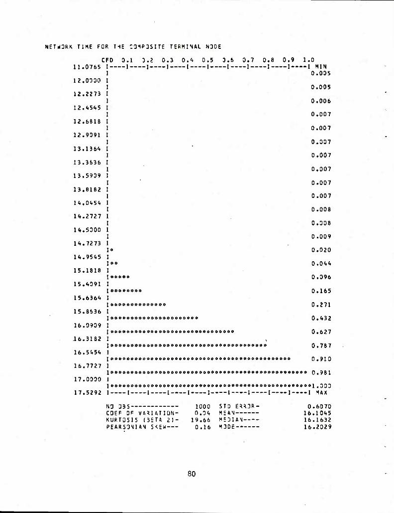
NETiORK TIME FDR HE C3iP3SITE TERMINAL N3DE

CFD 0.1 3.2 0.3 0.<* 0.5 3.S 0.7 0.8 0.9 1.0 11.0765 I 1 1 1 1 1 1 1 1 1 1 MIN

I 0.005 12.0300 I

I 0.005 12.2273 I

I 0.006 12.<>5<»5 I

I 0.007 12.6318 I

I 0.007 12.9091 1

I 0.307 13.136'- I

I 0.007 13.3636 I

I 0.007 13.5909 I

I 0.007 13.8182 I

I 0.007 lU.O'tS'-* I

I 0.008 1^.2727 I

I 0.008 1<».5DOO I

1 0.009 14.7273 I

I* 0.020 14.9545 1

I** 0.0'*'* 15.1818 I

!••*** 0.096 15.4091 I

I«»»«»««» 0.165 15.6364 I

I««o»»ooo««o»»« 0.271 15.8636 I

j««««»»«««o««o»«««oo««* 0.432 16.0909 I

Io»»«»««*«ft««o««««i««o««o«o»o««»« 0.62 7 .16.3182 I

l««0»oa»o««»«0«»»««oo#0»«o««»*»«»o«»«o«« 0.787 16.5454 I

IO«»O»«»«0»»»««OOO9OO»««*O««*»OO»O««*O»»«*««O» 0.910 16.7727 I

Ifto«o«o«ooo«»»«oo««»«»««oo*«o«»oo«oo«*«»«»oo«o«#«» 0.981 17.0000 I

] oooopao««.»*9oaotteei>i>o«*6»ai»»ooooaoooc>o»o»*»s9r>ooool .30 3 17.5292 I I 1 1 I 1 1 1 I 1 1 M4X

NO 33S 1000 STO E^3R- 0.6070 CQEF OF VARIATION- 0.34 MEAN 16.1045 KURTOSIS (3ETA 2)- 19.66 ME3IAN 16.1632 PEARS3NIAN S<EW— 0.16 M3DE 16.2029

80

PftTH COST FDR THE COMPDSITE TERMINAL NODE

82.<>0<>9

82.^.0^9

94.8342

107.2635

119.6927

132.1220

U4.5513

156.9806

169.4098

181.8391

194.2684

206.6977

219.1269

231.5562

243.9855

256.4146

268.8437

281.2729

293.7021

306.1313

318.5605

330.9397

343.4189

355.8491

355.8491

CFD 0.1 0.2 0.3 0.4 0,5 0.6 0.7 0.8 0.9 1.0 1 1 1 1 j 1 1 _i , j MIN

0.0

r)otKK>S)t> 0.131

0.580

0.720

0.923

0.923

0.923

0.923

0.923

0.923

0.923

0.928

0.944

ooa«6«*«*a»*e»»»e«ae«»«*(>«ae«*$#o««»o«a4fta**»$a* 0.957

»«»««»«««ao«oo»oo««««*eo»<r«»»»*«««»««o«««»««»««« 0.958

o««a«ao«t««««ci««»«««»««4t»o«>»««««««»#«o»««««»«»«*« 0.965

»««o««ioo««»«»a«#«ftcta»»oo»a»««»«»o»»o»»««»«#»o»«#» 0.980

»««oo6a«4ftci«ttO0a9««»«a0*o9 4««««t£eo«*aa£»ee««ee««4oQa999

«o*«o«o«a»o«««oo«o««»«a««oo»«»«»«»«««o»«a««o«o»oooo 999

««o«««ai»««««o«i>o«9»«»*»««(>«»«»««««4i»««0«#«»««o««««Q>999

1 i 1 j ! 1 j: j j j HAX

NO OBS 1000 STO ERROR- COEF OF VARIATION- 0.36 MEAN KURTQSIS (3ETA 2)- 11.38 MEOIAN PEARSDNUN S<EW 0.39 MODE

42.8560 117.8486 101.7044 101.1380

81

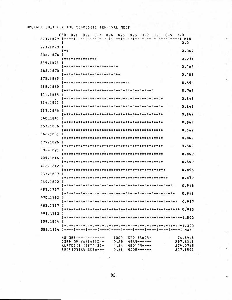
OVERALL CU5T FDR THE ZDiPDSITE TERMINAL NOPE

223.1879

223.1879

236.1876

249.1873

262.1870

275.1865

288.1860

301.1855

314.1851

327.1846

340.1841

353.1836

366.1831

379.1826

392.1821

405.1816

418.1812

431.1807

444.1802

457.1797

470.1792

483.1787

496.1782

509.1824

509.1824

0 0.1 0.2 0.3 0.'-* 0.5 D.6 3.7 0.6 0.9 1.0 1 1 i 1 1 1 1 1 1 1 MIN

0.0

OOOOOO 000 00000000 »o«o«o«oo«>«o«»«ooo«o««ooo«»*o«

o«oooo»»oooooooooooooo««ooooo#ooo«oo»ooo«oo*»o»o 0.9 57

OOOOOOOOOOOOOOO0000OOOOOOOOOO000000OOOOOOOOOAO^O^ 0.98 5

oot,ooi>oooo»ooo»oooooooooooo»ooooooooeor»oooooooooool,000

ooo«ooo»»oooooooooo«»eoo«oooo*ooooooooooo«o»o«««a»i.3Q0 1 1 1 1 1 1 J 1 1 1 MAX

0.044

0.271

Q.'+bU

0.468

0,552

0.762

0.3^5

0.849

0.849

0.849

0.849

0.849

0.849

0.649

0.S49

0.856

0.879

0.916

0.941

NO DBS 1000 STO ERR3R- COEF OF VMIftTlDN- 0.25 MEAN KURTOSIS (3cTfl 2)- 4.3^ MEDIAN PEA^SONIAN SKEH 0.68 MODE

74.5915 297.8311 279.0715 247.1503

82

PAl-H PERFORMANCE FDR THE C3>iP3SlTE TERMINAL NDDE

0.0

0.0

0.03^5

0.1689

0.253^

0.3379

0.^223

0.5068

0.5913

0.6757

0.7602

0.8^7

0.9291

1.0136

1.0980

1.1825

1.2670

1.351*

l.«i359

l.520<*

1.60<»8

1.6393

1.7738

1.8582

1.8582

CFD 0.1 0.2 0.3 O.i* 0.5 0.6 3.7 0.8 0.9 1.0 — _! 1 1 1 j j , , , j MIN

0.0

«««

o <> o

0.052

0.052

0.052

0.052

0.052

0.052

0.052

0.052

0.053

0.056

0.108

0.361

0.648

0.819

0.908

i>i>ooi>40os>!>os>i>»osoi>o<>op»c«=«5.ci>»i5i>*o»s>»*<.4ooo<>oe>ua 0.951

»»»o o«i>«*»s> ft*** oooo ■» ouoc wo ooo 9ao»»o o »ac* o o&ao* oo* Q 984

»«4i»«oo»»««««o««oo«««««»o«««««o«««««««««»««««»««0 0.990

ooooooooooooooooooooooooooooooooooooooooooooooooooO, 99^

ocooooooooeoooooooooooooooo«o»ooooooooooooooooooooo.998

oo»ooooo»ooooooooooooooooooooaoooaoooo*oooooooo«ool.033

OOOOOOOOOOOOOOOOOOOOOOOOOOOOOOOOOOOOOOOfOOOOOOOOOOl.OQO 1 1 ! ! , j , , j j •AX

NO DBS 1000 STD ERR0R- C0EF 3F VARIATION- 0.27 MEANr- KVJRTDSIS (BETA 2)- 10.56 MEDIAN PEARSD>IIAN SKEW 0.00 MODE

0.2779 1.0321 1.0548 1.0327

83

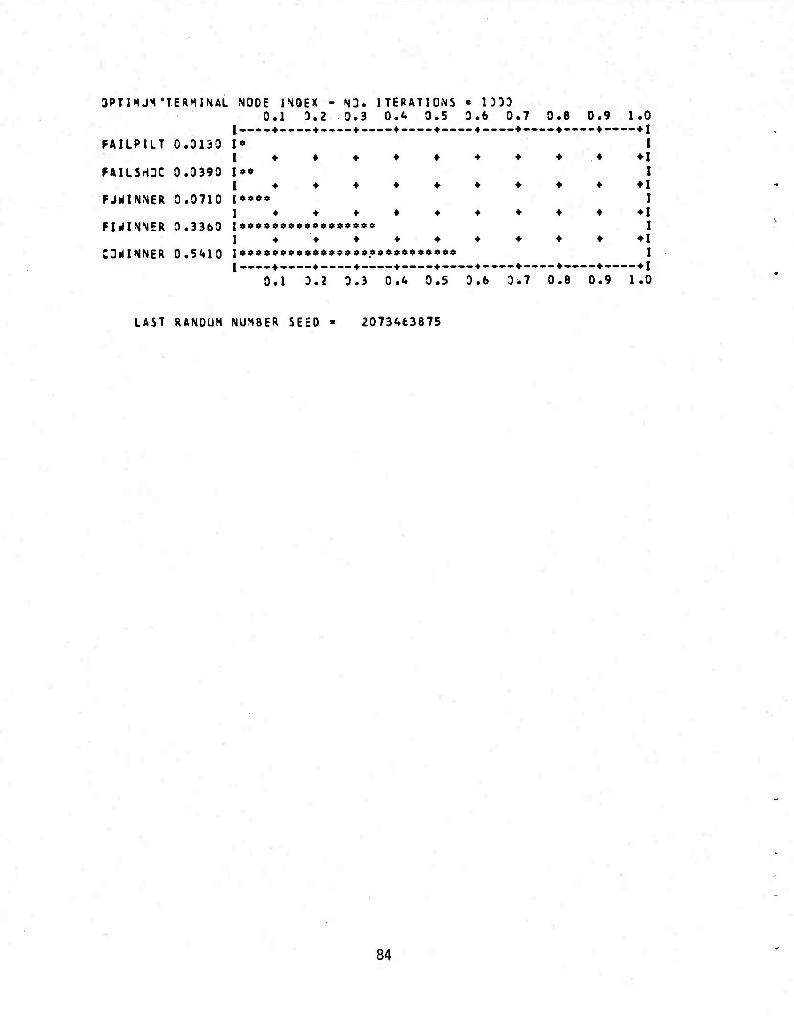
3PTIM.H'TEMINAL NODE l^OEX - N3. ITERATIONS « IDDD 0.1 0.2 0.3 O.A 0.5 0.6 0.7 0

{..^.^....^----♦- — -♦ —--4---'-'*>-•—♦-->•>

FAILP1LT 0.0130 I» !♦♦♦♦♦♦♦

FAILSrtOC 0.0390 I»» !■♦•♦♦♦♦♦♦

FJrflNNER 0.0710 !•••• !♦♦♦♦♦♦♦

FIrflNSER 0.3360 ]e0*«»«»*«*«9****e I ♦♦♦♦♦♦♦

COrilNNER O.S'tlQ ]«««>«««»*»«*«»»»«*«»»»«*««««

0.1 3.2 3.3 0.^ 0.5 3.6 3*7 0

S 0.9 1.0 ♦ ♦!

I ♦ ♦!

I ♦ ♦!

1 ♦ *l

I ♦ ♦!

I ♦ ♦! 8 0.9 1.0

LAST RANDOM NUMBER SEEO ' 2073463875

84

CHAPTER 6 AUXILIARY PROGRAM TO AID VERT

There is a peripheral program used to assist the VERT effort, program is known as DIMEN,which stands for dimensioning.

This

6-1. DIMEN - VERT's Core Storage Dimensioning Program

DIMEN dimensions VERT's storage arrays while simultaneously assigning compat- ible values to the check variables. These check variables are used to run a check on the quantity of Information being put in these storage arrays. If they have the same value as the magnitude of the storage arrays, these check variables will insure that the boundaries of these storage arrays are not exceeded when VERT loads these arrays. DIMEN was specifically structured to accomplish this logical task.

A. Definition of Inputs.

DIMEN requires only one input card which has the following layout.

Columns Format Check Variable Boundaries on the Check Variables# MlTEft.(ST.0.and.MITER.LT.lOOODO 1- 8 18

9-16 18

17-24 18

25-32 18

33-40 18

41-48 18

49-56 18

57-64 18

65-72 18

73-80 18

MARC

LARC

MNODE

LNODE

MTAG

MHIST

MTERM

MSLACK

MCPGAP

MARC.GT.O.and.MARC.LT.10000

LARC.GT.O.and.LARC.LT.100000

MNODE.GT.O.and.MNODE.LT.10000

(LNODE + MTAG).GT.O —and—

(LNODE + MTAG).LT.100000

MHIST.GT.O. and.MHIST.LT.100

MTERM.GT.O.and.MTERM.LT. 1000

MSLACK.GT.O.and.MSLACK.LT.1000

MCPGAP.GT.O.and.MCPGAP.LT.lOOO

# GT = Greater than and LT = Less than

B. Example Output.

OCOMMDN/A^CS/aSFD^ 20r0 1 ,UT IME 4 ( 125),TIMEM 125>,UC35TA( 125), SLH 710 lCOSTft( 125),JPE5F4( 125),PERFA( 125),W3RK( 125),1STAT£( 125), GLM 720 2N00EI( 1251,MnD£3( 125),1CR1TA( 125),KEEPC( 1 25 ) , KEEPP ( 125), OLI 730 3IARC1( 125),IARC2( 125),1PD1NT( 125),JPDINT( 125),ISLAM 125), GLM 7^.0 4<ARC,LMC,-lARC,NAi?C, ITALCITALP ,ISTAR GLM 750 OCOMMOVTRIALS/STl^ET ( 500,^),TERM 2,8),KP01NT( 2),NO0ET( 500), GLM 960 1MT£RM,STE^,M TE^ , 1TER 3LM 970 0COMMON/AR:S/ASr3^E( 2nC0),UTIMEA( 125),T1MEA( 125),UCOSTA('125), GLM 980 1CDSTA( 125),JPERFA( 125),PERFA( 125),WORM 125),ISTATE( 125), GLM 990

85

2NG0EI( 125),S3D£ 3IARCH 12S)fIAAC ^ARC.LARC ,1ARC,N OCaiMQN/NDOES/TM 1N3DE1( 75),N:D£ 2NARCI( 75),NA?C 3NPGINH 75),NSL ^^TAG OCDMMON/HIST/XMIN

D{ 125),ICRITA( 2( 125),IPD1NT( ARC,lTALCt ITALP EN( 7b),COSTN( 2( 75),L3GI( 3( 75),ISTAT( A<( 75.),JUMP(

125),KEEPC( 125),KEEPP( 125), 125),JP31NT( 125),ISLAM 125), ,ISTAR 75),PERFN( 75),NSTDRE( 1203),

75),L3GD( 75),MSTATE{ 75), 75),INSTAT( 75),ICRITN( 75), 75),KNDDE,LNaC£,MNa0E,NN0DE,HTAC,

1HAVE( OCOMMUN IJOBSl OCDMMON 1CHMAX« 2PAVE(1 ilTER MARC LARC MNJDE LN3DE HTAG MHIST MTERM MSLACK MCPGAP

OCOMMON MTERM, OCQMMDN 1MTERM, OCOMMON 1C3STA( 2N30EI( 3IARC1( '►KARCL OCOMMON 1N3DE1( 2NARCI( 3NP0INT '.^TAG OCOMMON 1HAVE( OCOMMON 1J0BS( OCOMMON 1C0STA( 2N3DE1 « 3IARC1( <»<ARC,L OCOMMON 1MTERM, OCOMMON 1C0STA( 2N0DEI ( 3IARC1( <»KARC,L OCOMMON 1N00EH 2NARCI ( 3NPQ1NT ^NTAG 0C3MM0N HAVE(

/SLAC b) ,MS /CPGA 10),C D) ,KC « 5D - 12 ' 203

7 * SD « 63

1 /TRIA NTE^M /TRIA NTERM /ARCS 125) 125) 125)

ARC,1 /NOD?

75) 75)

( 75

/HIST ^)t /SLAC 8),MS /ARCS 125) 125) 125)

ARC,M /TRIA NTERM /ARCS 125) 125) 125)

ARC,M /NODE

75) 75)

( 75

IOBS( K/RMI LACK, P/T1( AVEU OBSd 0 5 0 5 3 0

2 8 0 LS/ST ,MITE LS/ST ,MITE /ASTD ,JP£R ,N33£ ,IARC ARC,N S/TIM ,N03£ ,NARC ),NSL

/XMIN lOBSC K/RMI LAC<, /ASTO ,JP£R ,N3DE ,IA<C ARC.N LS/ST ,M1TE /AST3 , JPrR ,N33£ ,1 A^C ARC.N S/TIM ,N3D£ ,NARC ) ,NSL

( ^,<»),XMAX( 4,4),HMIN( ^,<»),HMAX1 <»,<.),

<») ,MHIST,NHIST N( 8),RMAX< 8),SMIN( 8),SMAX( 8),SAVE! 8), NSLACK 10),T2(1C),CSMIN(10),CSMAX(13),CHMIN(10), 0),PSMINnO),P5MAX(10),PHMIN(lD) ,PHMAXI10), 3),KP0bS(lG),MCPGAP,NCP5AP,ICP0AP

(

500,A),TERM( 2,8),KP0INT( 2),NDDET( 500),

500,4),TERM( 2,8),KP01NT( 2),N0DET( 500),

3RET( R,1TER 3RET( R.ITER RE( 2000),UTIMEA( 125),TIMEA( 125),UC0STA( 125), PA( 125),P£RFA{ 125),W3RK( 125),ISTATE( 125), 0( 125),ICR1TA( 125),K£EPC( 125),KEEPPI 125), 2( 125),IPDINT( 125),JP3INT( 125),ISLAK( 125), ARC,1TALC,ITALP,ISTAR £N( 75),C0STN{ 75),PERFN{ 75)fNST0RE( 1233), 2( 75),L3GI( 75),La&3( 75),N5TATE( 75), 3( 75),ISTAT( 75),INSTAT( 75),ICRITN( 75), AK( 75)fJUMP( 75),KN00E,LNaDEfMN0DE,NNaDE,MTAG,

( 4»4)tXHAX( 4,<»),rtMIN( <»,4),HMAX( 4,4), i»),MHIST,NHlST

N{ 8),RMAX( 8),SM1N( 8),SMAX( 8),SAVE! 8), NSLACK RE( 2000),UTIMEA( 125),TIMcA( 125),UC0STA( 125), FA( 125),PERFA( 125),H3RK( 125),ISTAT£( 125), 0( 125),ICRITA( 125),KEEPC( 125),KEEPP{ 125), 2( 125),IP0INT( 125),JP0INT( 125),ISLAK( 125), ARC.ITtLC ,ITALP,ISTAR 3RET( 500,4),TERM( 2,8)tKP0INT( 2),NaDET( 500), R.ITER RE( 2300),UTIMEA( 125),TIMEA( 125),UCaSTA( 125), FA( 125),PERFA| 125),tf3RK( 125),ISTAT£( 125), 31 125),ICRITA( 125),KEEPC< 125),K£EPP( 125), 2( 125),IPDINT( 125),JP0INT( 125),ISLAK( 125), ARC,ITALC,ITALP ,ISTAR EN( 75),CQSTN( 75),PERFN( 75),NST0RE( 1203), 2( 75),LBGI( 75),LaG3( 75),NSTATE( 75), 3( 75),ISTAT( 75),1N5TAT( 75),ICRITN( 75), A<( 75),JUMP! 75)fHN03E,L.N0DE ,MN00E ,NNOOE,MTAG,

/HIST/XMIN( 4,4),XMAX( ^,^),-)MIN( 4t4)tIQBS( «») ,MHI5T,NHIST

4,4),HMAX< **,<,)

GLM GLM GkH SLM GLM GLM GLM GLM GLM

GLM GLM GLM GLM GLM GLM GLM GLM GLM GLM GLM GLM GLM GLM GLM GLM GLM GLM GLM GLM GLM GLM GLM GLM GLM GLM GLM GLM GLM GLM GLM GLM GLM GLM GLM15^10 GLM15^20 GLM15430 GLM^-UO GLM1545J GLM15790 GLM15800 GLM15810 GLM15823 GLM15830 GLM158^0 6LM15850 GLM15863 GLM15870 GLM15880 &LM15893 GLM15895 GLM15900 GLM15910

1000 1010 1020 1030 lO'.O 1050 1060 1065 1070

1080 1090 1100 1110 1120 1130 2090 2100 2110 2120 2130 2140 2150 2160 2173 2180 8920 8930 9260 9270 9280 9290 9303 9310 9320 9330 93^0 9350 9360 9365 9373 9380 9390 9400

86

OCOMMQN/SLftC</RHlN{ 8),RMAX( 8),SMIN( 8),SMAX( 8),SAVE( 8), lJOeS( 8),HSLftC<,MSLACK

0C0HM0N/CPSftP/Tl(lD),T2(10),CSMIN(10»,CSiAX(10)fCHMIN(10)f

ICHMAX(IO),CAyE(10),PSMlN(10),PSMAX(10),PHMIN(10),PHMAX(10», 2PAVE (10),'<C03S(10),KPDPS(10),MCP&AP,NCPGAP,ICP&AP OCOMMON/TRIALS/STDREK 50Dt^)tTERH( 2,B),KPOINT( 2),NaDET( 500) 1MTER*1,NT£IH,'1ITE*,ITER OCOMMON/ARCS/ASTORE( 2000 ) ,UT 1ME A( 125),TI»1EA( 125),UCDSTA( 125), 1C0STA( 125),JP=RFAI 125),PERFA( 125),WaRK( 125),1STATE( 125), 2S0DEI( 125),NaOE3( 125),ICRITA( 125),KEEPC( 125),KEEPPJ 125), 31ARC1( 125),mC2( 125),IP0INT( 125),JPD1NT( 125),ISLAK( 125), '.KARCLARC'iARCNARCITALCITALP.ISTAR DC0HH0N/M3DSS/TME1I 75),COSTN( 120D)

75) ,N3DE2( 75),NA<CD(

75),NSLAK(

75),LOCK 75),ISTAT(

75) ,JUMP(

75),LDGa( 75),M5TATE( 75), 75),INSTAT( 75),ICR1TN( 75), 75),KNaOE,LNDDE,MNaDE,NNQDE,,1TAG,

<»,<»>,HMAX( 4,4),

8) ,SAVE( 8) ,

75),PERFN( 75),NST0RE(

INODEK 2NARCI < 3NP3INT( <iNTAO OCOH^QN/HISr/XMIN( 4,4),XMAX( 4,4),HM1N( 1HAVE( ^,4),1QBS( 4),MH1ST,NHIST 0C0MM0N/SLAC</R»1IN( 8),RMAX« 8),SM1N( 8),SMAX( 1J38S( 6) ,MSLAC<,NSLACK 0C0MMDM/CPGaP/TI(10),T2(10),CSMIN(n),CS1AX(lD),CHMINn0), ICHMAX(IO) ,CAVE(lD),PSMlNllO),PSMAX(10),PHMlN(n) ,PHMAX(10), 2PAVE(10),<:D3S(10),KP3fcS(lO)fMCP&AP,^CPGAP,ICPGAP

DMENS1DM SL4C<A( 125), SLACKNC 75), IPATHA( 125), 1PAHN( 75) 0CDMMDN/A^CS/AST3RE< 2000 ) ,UT 1 ME A ( 125),rMEA( 125),UC0STA( 125), 1C0STA( 125),JPERFA( 125),PERFA( 125),WORM 125),ISTATE( 125), 2NaOEI( 125),«J3:ED« 125),ICRITA( 125),KEEPC( 125),KEEPP( 125), 3IARC1( 125),mC2( 125),IPD1NT( 125),JPDINT( 125),ISLAK( 125), <.<ARC,LARC,«URC,NARC,ITALC,ITALP,ISTAR 0C0MMDN/l«30ES/THgN| 75),C0STN( 75),PERFN( 75),NSTDRE( 1200), INODEK 75),ND3E2( 75),L3&I( 75),LDG3( 75),^STATE< 75),

75),I5TAT( 75),INSTAT{ 75),ICR1TN( 75). 75) ,'4A^C3( 75),^SLA<( 75), JUMP( 75),KN3DE,LNQDE,MN00E,NN0DE,MTAG,

2WARCI ( 3>IP01NT( 4NTAG

0COMMDN/ARCS/AST3RE( 20C0 ) ,UTIMEA» 125)fTIMEA( 125),UC0STAI 125), 1C0STA( 125),JPERFA( 125.),PERFA( 125),W3RK( 125),ISTATE( 125), 2N00EI( 125),N33E3( 125),ICRITA( 125),KE£PC( 125),KEEPP( 125), 3IARC1( 125),URC2( 125),IPD1NT( 125),JPDINT( 125),I5LAK( 125), ^KARCLARC^ARCNARCITALCITALP^STAR OCOMMON/^DOES/TIMENt 75),CaSTN( 75),PERFN( 75),NSTDRE( 1233), INODEK 75),M3DE2l 75),L0GI( 75),L0GD( 75),^5TATE( 75), 2MARCI( 75),NARC0( 75),1STAT( 75),1NSTAT( 75),ICRITN{ 75), 3NP0INT( 75),NSLA<( 75),JUMP( 75 ), K,43DE ,LN3CE ,MNODE ,NNODE ,MT AG , 4NTAG 0CDMM0N/ARCS/AST3RE( 2000 ) ,UT1ME A( 125),TIMEA( 125),UC0STa( 125), 1C0STA( 125),JPERFA( 125)fPERFA( 125),W3RK( 125),ISTATE( 125), 2N0DEI( 125),N33E3( 125),1CRITA( 125),KEEPC( 125),KEEPP( 125), 3IARC1( 125),IA^C?( 125),IP0INT( 125),JPDINT( 1?5),I5LAK{ 125). ^KARC.LARC^A^CVARCITALC.ITALP^STAR OCOMMON/NODES/TIMENI 75),CaSTN( 75),PERFN( 75),NST0RE( 1200). INODEK 75),\I33E2{ 75),LaGI( 75),LQG3( 75),,JSTATE( 75),

75),15TAT( 75)fINSTAT{ 75),ICRITN( 75), 75),JUMP( 75),KN3DE,LN0CE,MN0DE,NN0DE,MTAG,

75) ,NA^C3( 75 ),NSLA<(

2NARCI( 3NP0INT( <,NTAG

0C0MM0N/ARCS/AST3RE( 2000),UTI ME A( 125),TIMEA( 125),UC0STA( 125). 1C0STA( 125),JPERFA( 125),PERFA( 125),W3RK{ 125),1STATE( 125), 2N0DEI( 125),>133£3( 125),1CRITA( 125),K£EPC( 125),KEEPP( 125), 31ARCK 125),1ARC2( 125),IP01NT( 125),JP3INT( 125),ISLAK( <KARC,LARC,iARC,NARC,lTtLC,ITALP,ISTAR 0C0MM0N/V(3DES/T1MEN( 75),CD5TN( 75),PERFN{ 75).NST0RE( 120D) INODEK 75),N3DE2| 75),L3GH 75),LaG3( 75),V5TATE( 75),

125)

GLM15920 &LM15930 &LM15932 &LM15934 GLM15936 GLM20940 GLM20950 GLM20960 GLM20970 GLM20980 GLM20990 GLM21000 &LM210in

&LM21020 &LM21030 GLM21040 GLM21045 6LM21050 &LM21060 GLH21070 GLM21080 GLM21090 GLM21100 GLH21110 Gm21120 GLM33250 GLM33260 GLM33270 GLM33280 GLM33290 GLM333C0 GLM33310 GLM33320 GLM33330 GLM33335 GLM33550 GLM33560 GLM33570 GLM335e0 GLM33590 GLM33600 GLM33610 GLM33620 GLM33630 GLM33635 GLM3^26G GLM34270 &LM34280 GLM34290 GLM34300 GLM34310 GLM34320 GLM34330 GLM3<.340 &LM34345 GLM34650 GLM34660 GLM3^670 GLM34680 GLM3<,690 GLM34700 &LM34710

87

2NARC1( 75)tM4-lCJ( 7!>),ISTAT( 75),I^srAT( 7%),KKITN( fb) , JL«iJ'.7<;o 3NP0INT( 75),NSLA'<( 75),JUMP( 75 ) .KNQDE ,L NODE , MNODE , NNGOE , S T AG , &LM^l7?0 <.NTAC OL1J'.7jrk 0CDMM0N/A^CS/4ST3H£( 2300) ,UT1M=A( 125),TIMEA( 125),UCDSTA( 125), iLM353lO IC0STA( 125),JPERF41 125),PERFA( 125),W3RK( 125)fI5TATE( 125), &LM35320 2N0DEI( 125),Na3ED( 125),ICRITA( 125),KEEPC( 125),KE£PP( 125), GLM35330 31ARC1( 125),mC2( 125),IPDIMT{ 125),JP3INT( 125),1SLAK( 125), 5LH353<»0 fc<A«C,LARCt1A*C»MARC,lT*LC»ITAL»f1STAR &LM3535 0 OCO^MON/NDDES/TMEMC 75),C0STN( 75),PERFN( 75),N5T0RE( 1203), &LM35360 INOOEK 75),,433E2( 75),L0&I( 75),L0&a( 75),N5TATE( 75), GLM35370 2SARCn 75),NA^C3< 75),ISTAT( 75),INSTAT( 75),ICRITN( 75), GLM35380 3NP3INT( 75),NSLA<( 75),JUMP< 75),KN03E .LNQtE,MNOCE,NNO0£,11AG, GLM35390 <»NTAG GLM35395 OCOMMON/ARCS/ASTDREC 2000),UT1 ME A( 125),TlMEAt 125),UC0STA( 125), GLH357^0 1C0STA( 125),JPERFA« 125),PERFAl 125),W3RK( 125),ISTATE( 125), GLM35750 2N0DE1( 125),S3DE3( 125),ICRITA( 125),KEEPC( 125),KEEPP( 125), GL,135760 31ARC1( 125),IA^C2( 125),1P0INT( 125),JP3IHTJ 125),ISLAK( 125), GLM35770 <»KARC ,LARC,1ARC,NARC,ITALC,1TALP,ISTAR ' GLM35780 0C0M*1QN/N30ES/TMEN« 75),CD5TN( 75),PERFN( 75),NSTDRE( 1200), GLM35790 1N33£1( 75),^03E2( 75),L0&I( 75),LDG0( 75),NST4TE( 75), GLM35800 2NARCI( 75),MA<C3( 75),ISTAT( 75),1NSTAT( 75),ICRITN( 75), GLM35810 3NP31NT( 75),MSLAK( 75),JUMP( 75),KN33£,LNDDE.MNODE,NNO0E,MTAG, &LM35820 «.NTAG GLM35825 0C0MM3N/TRULS/ST3RET( 500 , ^ ) ,T ERI { 2,8),KPaiNT( 2),N00ET( 500), GLM43050 IMTcftM,NTEÎ,MITER,ITER &LM<,0060 0CaMMDN/ARCS/AST3^£( 2000 ) ,UT I ME A( 125),T1MEA( 125),UCaSTA( 125), GLM<,0070 1CDSTA( 125),JPERFA( 125),PEKFA( 125),W3RK( 125),ISTAT£( 125), GLM40080 2N00EI( 1?5),N3DE3( 125),ICRITA( 125),ÊEPC( 125),KE£PP( 125), GLM^0090 31ARC1( 125),IARC2( 125),IPD1NT( 125),JP01NT( 125),1SLAK| 125), GLMÔIOO 4'<ARC,LASC,HARC,NARC,ITALC,ITALP ,ISTAR GLM40110 aCOMHON/NDOES/TMSNI 75),C0STN( 75),P£RFN( 75),NSTDRE< 1203), GLM40120 INOOEK 75),S33£2( 75),LrJ&I( 75) ,LDG3 < , 75) ,NST ATE ( 75), GLM40130 2NARC1( 75),NA*C3{ 75),ISTAT( 75),INSTAT( 75),1CRITN( 75), &LM40140 3MPD1NT( 75),NSLA<( 75),JUMPl 75 ) ,KNDOE .LNDDE,MNODE,NNODE,MTAG, GLMÔISO WtM GLM40155 0C0MMDN/HIST/X^1N( 4,A),XMAX( <,(4},HMIMi 4,4)fHMAX( A,<,), GLM40163 1HAVE( i*,t*),\QBS( ^) tMHl5T,NHI5T GLM40170 OCOMMON/SLACK/Rim B)tkMAX( 8),SMIN( 8),SMAX( 8),SAVE( 8), GLM40180 1J0BS( 8) ,HSLAC<,NSLACK &LM40190 OCOMMON/CPGAP/T1(10),T2(10),CSMIN(10),CSMAX(10),CHMIN(10), GLM402 03 1CHMAX(10) ,CAV£(10) ,PSMIN(10),P5MAX(10),PriMIN(10),PHMAX(10), GLM40210 2PAVE(10) ,'<:03S(10),KPaBS(10),MCPGAP,NCPGAP,ICPGAP GLM40220 CQMMDN/MEDAN/Z( 500 ) , XMED .KDU^T GLM40230 ODIMENSm HSTD(n,4), HTOSdO,^), HI ST (1 0 ,4 ,29 ) , ABSA(IO), &LM40240 COMMDN/MEOAN/Z( 500 ) , XMEO , KQUNT GLMA5910

0C0MMDN/TRI4LS/ST3R£T( 500,M,TER»1( 2,8),KP0INT( 2),NDDET( 500), GLM46320 1MTERM,NTE^,MITER,ITER GLN46330 CDMMDN/HED4N/Z( 500 ) ,XME 0 .KOUMT GLM463f. '

0C0MMDN/CPG4P/T1(10),T2 110),CSMIN(10),CSMAX(10),CHMIN(10), GLM47160 lCHMAX(13)fC4VE(13),P5MlN(10),PSMAX(10)tPHMIN(10),PHMAX(10), GLM47170 0CDMM0N/TRIALS/ST3RET( 503 ,4),TERM( 2,8),KPaiNT( 2),N0DET( 500), GLM46640 lMTERM,NT5R%1ITERflTER GLM48650 OCOMMDN/ARCS/ASTDRE( 2000) ,UTI ME A( 125),TIMEA( 125),UCaST4( 125), GLM48660 1C05TA( 125),UPERFA{ 125),PERFA( 125),wa^K( 125),ISTATE( 125), GLM48670 2N0DEn 125),N3DE3( 125),1CRIT6{ 1?5),KEEPC{ 125),KEEPP( 125), GLM48680 3IARC1( 125),IA^C2( 125),IP0INT( 125),JP3INT( 125),ISLAK( 125), GLM48690 4KARC,LARC,MARC,NARC,1TALC,1TALP,ISTAR GLM48700 OCDMMDN/NOOES/TIMENC 75),C0STN( 75),PERFN( 75),NSTQRE{ 1200), GLM48710 INOOEK 75),^33E2( 75),LDGI( 75),LaG0( 75),NSTATE( 75), GLM48720 2NARCI( 75),MA<C3( 75),ISTAT( 75),INSTAT< 75),ICRITN( 75), GLM(>9730 3NP0INT( 75),NSLAK( 75),JUMP( 75J,KNODE,LNDDE,MNaOE,NNDOc,iTAG, GLM43740 *NTA& GLM48745

88

Department of the Navy

Office ot AssibLdnt bei-retciry or the Navy (I&L)

ATTN: Dir, Ordnance Programs Washington, DC 20360

Chief of Naval Operations Washington, DC 20350

ATTN; 0P411 0P0411C

Commandant US Marine Corps ATTN: LMG Washington, DC 20380

Chief Naval Material Command Washington, DC 20362

ATTN: MAT-02 MAT-0242D

Commander Naval Sea Systems Command ATTN: 64D Washington, DC 20362

Commander Naval Air Systems Command Washington," DC 20361

ATTN: AIR-05 AIR-541

DISTRIBUTION LIST

UepdrLinoriL ot Lite Army

(1)

(2)

(1)

(2)

Commander Naval Supply Systems Command NAVSSC Code 042 Rm 706 Crystal Mall 3 Washington, DC 20376

Commander Naval Facilities Engineering Command NAVFAC Code 202A Washington, DC 20390 (1)

Commander Naval Weapons Station Earle Colts Neck, NJ 07722

Urrice or trie Assistant Secretary or the Army

(Research, Development & Acquisition] Washington DC 20310

Office DCS Research, Development & Acquisition

Washington, DC 20310

ATTN: DAMA-CSM DAMA-CSM-P DAMA-CS2-A

Commander US Army Materiel Development &

Readiness Command Alexandria, VA 22333

ATTN: CRCPA CRCCP CRCPP DRCSA-JS DRCLS

Commander US Army Armament Materiel Readiness

(1) Command Rock Island, IL 61299

ATTN: DRSAR-DA DRSAR-AS (2) DRSAR-PP DRSAR-TM

DRSAR-PC DRSAR-PE DRSAR-PD DRSAR-MS DRSAR-IR DRSAR-IL DRSAR-MA DRSAR-CP DRSAR-LE DRSAR-MM DRSAR-QA

Industrial Base Engineering Activity ATTN: DRXIB-IP

(1) Rock Island, IL 61299

(1)

Commander Harry Diamond Laboratory Washington, DC 20783

HQ JUSMAG-K (Box 11) ATTN: MKL0-S AP0 San Francisco 96309

(1)

(3)

(5)

(15)

(D

(1)

(1)

Department of the Army (Cont'd) Department of the Air Force (Cont'd)

Commander US Army Logistics Center ATTN: ATCL-CG Ft. Lee, VA 23801 (1)

Commander US Army Armament Research &

Development Command Dover, NJ 07801 (1)

Commander US Army Research Office P.O. Box 12211 Research Triangle Park, NC 27709 (1)

Director Mathematics Research Center University of Wisconsin-Madison 610 Walnut Street Madison, Wisconsin 53706 (1)

Director Army Materiel Systems Analysis

Agency ATTN: DRXSY-DI Aberdeen Proving Grounds, MD 21005(1)

Department of the Air Force

Office of the Assistant Secretary of the Air Force (I&L)

ATTN: SAF/ILP Rm 4D862 Pentagon Washington, DC 20330 (1)

Deputy Chief of Staff System & Logistics

Rm 4E262 Pentagon Washington, DC 20330 (3)

ATTN: AF/LE AF/LEYW AF/LEYWC

Deputy Chief of Staff R&D Washington, DC 20330

ATTN: AF/RDQ AF/RDP

(2)

Commander Air Force Systems Command Andrews AFB, MD 20331 (2)

ATTN: SDZA JTCG/MD

Commander Air Force Logistics Command Wright-Patterson AFB, OH 45433 (5)

ATTN: MMWM XR XRX XRP L0 L0WM

Commander Ogden Air Logistics Center ATTN: MMO Hill AFB, UT 84406 (1)

Commander Armament Development & Test Center ATTN: SDC Eglin, AFB, FL 32542 (1 )

Commander Aeronautical Systems Division Wright-Patterson AFB, OH 45433 (1)

Office, Secretary of Defense

Office of Director of Defense Research & Engineering

Washington, DC 20301 (2)

ATTN: Standardization and Support, Rm 2A318 Pentagon

Ammunition Programs, Rm 2B284 Pentagon

Defense Logistics Agency

Commander Defense Fuel Supply Center Cameron STation Alexandria, VA 22314 (1 )

Defense Logistics Agency (Cont'd) Service Schools (Cont'd)

Director of Procurement . DSA HQ Cameron Station Alexandria, VA 22314 (1)

DoD Information Distribution

Defense Documentation Center Cameron Station Alexandria, VA 22314 (1)

JCAP Coordinating Group

Executive Director, JCAP/CG Rock Island, IL 61299

Service Schools

Industrial College of the Armed Forces Ft. Leslie J. McNair Washington, DC 20319

National War College Ft. Leslie J. McNair Washington, DC 20319

Armed Forces Staff College Norfolk, VA 23511

Naval Postgraduate School Monterey, CA 93940

US Air Force Air University Maxwell AFB, AL 36112

Defense System Management College Ft. Belvoir, VA 22060

Army War College Carlisle Barracks

. Carlisle, PA 17013

Superintendent , US Military Academy

ATTN: COL A. F. Grum West Point, NY 10996 (1)

Conwander US Army Logistics Management Center Ft. Lee, VA 23801 (5)

Service Project Managers, Department of Navy

Commander Naval Air Systems Command Washington, DC 20361

ATTN: PMA PMA PMA PMA

231 234 235 240

(10)

es

PMA PMA PMA PMA PMA PMA PMA PMA

241 242 244 253 255 257 258 259

PMA PMA PMA PMA

261 262 264 265

PMA PMA PMA

266 269 270

PMA 271

Commander Naval Sea Systems Command Washi ngton. , DC 20362

ATTN: PMS 266 PMS 395 PMS 300 PMS 396 PMS 301 PMS 397 PMS 303 PMS 399 PMS 304 PMS 402 PMS 306 PMS 400 PMS 307 PMS 404 PMS 376 PMS 405 PMS 377 PMS 406 PMS 378 PMS 407 PMS 383 PMS 389 PMS 392 PMS 393

(20)

(24)

Service Project Managers Department of Navy (Cont'd)

Director Strategic Systems Project HQ Naval Material Command Washington, DC 20360 (5)

ATTN: PM2 JPM 3 PM 4 PM 5 PM 22

Service Project Managers Department of Army

Commander US Army Materiel Development Readiness Cmd ATTN: DRCPM-CS 5001 Eisenhower Avenue Alexandria, VA 22333 (1)

Commander US Army Materiel Development & Readiness Cmd ATTN: DRCPM-MEP 7500 Backlick Road Springfield, VA 22150 (1)

Commander US Armv Materiel Develooment & Readiness Cmd ATTN: DRCPM-ARD

DRCPM-TND Naval Equinment Training Center Orlando, PL 32813 (2)

Commander US Armv Armament Materiel ATTN: "DRCPM-M110E2 Rock Island, IL 61299

Readiness Cmd

(1)

Commander US Army Armament Research & Development Cmd ATTN: DRCPM-AAH-30MM

DRCPM-ADG DRCPM-CAWS DRCPM-CAWS-GP DRCPM-NUC DRCPM-PBM DRCPM-SA

Dover, NJ 07801 (7)

Service Project Managers Depart lent of Army (Cont'd)

Commander US Armv Aviation Research & Development Cmd ATTN: DRCPM-AAH

DRCPM-ASE DRCPM-BH DRCPM-CH47M

P.O. Box 209 St. Louis, MO 63166 (4)

Commander US Army Communications & Electronics

Materiel Readiness Cmd ATTN: DRCPM-NC

DRCPM-SIEW Ft. Monmouth, NJ 07703

Commander US Army Communications Research &

Development Cmd ATTN: DRCPM-ATC

DRCPM-ATTS DRCPM-COM DRCPM-FF DRCPM-GARS DRCPM-MSCS DRCPM-RBS DRCPM-SC DRCPM-STA DRCPM-TDS DRCPM-TDS-PL DRCPM-TDS-TF DRCPM-TDS-TOS

Ft. Monmouth, NJ 07703

(2)

(13)

Commander US Army Electronic Materiel Readiness Cfnd ATTN: DRCPM-CAC Vint Hill Farms Station Warrenton, VA 22136 (1)

Commander US Army Mobility Equipment Research and

Develooment Cmd ATTN: DRCPM-FM Ft. Belvoir, VA 22060 (1 )

Service Project Managers Department of Army (Cont'd)

Commander US Army Missile Materiel Readiness Cmd ATTN: DRCPM-CF

DRCPM-DT DRCPM-HA DRCPM-KMS DRCPM-LC

Redstone Arsenal, AL 35S09 (5)

Commander US Army Missile Research & Development Cmd ATTN: DRCPM-HEL

DRCPM-HF DRCPM-LD DRCPM-MD DRCPM-MP DRCPM-PE DRCPM-RK DRCPM-ROL DRCPM-RS DRCPM-TDS-RA DRCPM-VI

Redstone Arsenal, AL 35809 (11)

Service Project Managers Department of Army (Cont'd)

Commander US Armv Aberdeen Proving Ground ATTN: DRCPM-DR

DRCPM-SMK Aberdeen Proving Ground, MD

Service Project Managers Department of Air Force

Armament Directorate A-10 System Program Office ATTN: " ASD/YX Wright Patterson AFB, OH 45433

Commander ASK/01 Wright-Patterson AFB, OH 45433

Commander SAMSO/OI Los Angeles AFS, CA 90009

(2)

(1)

(10)

(10)

Commander US Army Tank-Automotive Materiel Readiness ATTN: DRCPM-CE Cmd.

DRCPM-FVA DRCPM-FVS DRCPM-HT DRCPM-M60TD DRCPM-M60TP DRCPM-MTIS

Warren, MI 42090 (7)

Commander US Army Tank-Automotive Research and

Development Cmd. ATTN: DRCPM-CVT

DRCPM-GCM DRCPM-ITV

Warren, MI 48090 (3)

Commander ESD/OI Hanscom AFB, MA 01730

Commander AFGL/OI Hanscom AFB, MA 01730

Commander AMD/01 Brooks AFB, TX 78235

Commander AFHRL/OI Brooks AFB, TX 7823 5

(10)

no;

(10)

(10)

Commander US Army Troop Support & Aviation Materiel

Readiness Cmd. ATTN: DRCPM-AE

DRCPM-AWC DRCPM-CO DRCPM-IAP

4300 Goodfellow Blvd St. Louis, MO 53120 (4)

Commander ADTC/OI Eglin AFB, FL 32542 (10)

Service Project Managers Department of A1r horce '(Cont'd)

Commander SAMTEC/OI Vandenberg AFB, CA 93437 (10)

Commander AEDC/OI Arnold AFS, TN 37389 (10)

Commander AFFTC/OI Edwards AFB, CA 93523 (10)

Commander AFRPL/OI Edwards AFB, CA 93523 (10)

Commander AFWL/OI Kirtland AFB, NM 87117 (10)

VENTURE EVALUATION AND REVIEW TECHNIQUE (VERT) … · 2015-06-25 · 1-2 VERT History 2 2 The VERT...

Documents

Transcript of VENTURE EVALUATION AND REVIEW TECHNIQUE (VERT) … · 2015-06-25 · 1-2 VERT History 2 2 The VERT...