* Corresponding author. Tel: +9821-88021067/ Fax: +9821-88013102 E-mail address: mrabani@ut.ac.ir (M. Rabbani) © 2018 Growing Science Ltd. All rights reserved. doi: 10.5267/j.dsl.2017.4.006

 

  

Decision Science Letters 7 (2018) 25–38

Contents lists available at GrowingScience

Decision Science Letters

homepage: www.GrowingScience.com/dsl

Vendor managed inventory control system for deteriorating items using metaheuristic algorithms

Masoud Rabbania*, Hamidreza Rezaeia, Mohsen Lashgarib and Hamed Farrokhi-Aslb aSchool of industrial Engineering, College of Engineering, University of Tehran, Tehran, Iran bSchool of Industrial Engineering, Iran University of Science & Technology, Tehran, Iran

C H R O N I C L E A B S T R A C T

Article history: Received September 16, 2016 Received in revised format: October 22, 2016 Accepted April 29, 2017 Available online April 30, 2017

Inventory control of deteriorating items constitutes a large part of the world’s economy and covers various goods including any commodity, which loses its worth over time because of deterioration and/or obsolescence. Vendor managed inventory (VMI), which is a win-win strategy for both suppliers and buyers gains better results than traditional supply chain. In this research, we study an economic order quantity (EOQ) with shortage in form of partial backorder under VMI policy. The model is concerned with multi-item subject to multi-constraint including storage space, time period and budget constraints. Two metaheuristic algorithms, namely Simulated Annealing and Tabu Search, are used to find a near optimal solution for the proposed fuzzy nonlinear integer-programming problem with the objective of minimizing the total cost of the supply chain. Furthermore, the sensitivity analysis of the metaheuristic parameters is performed and five numerical examples containing different numbers of items are conducted in order to evaluate the performance of the algorithms.

Growing Science Ltd. All rights reserved.8© 201

Keywords: Vendor managed inventory Economic order quantity Fuzzy Metaheuristic algorithm Deteriorating items

1. Introduction

Importance of inventory cost is as much as pretax operation profits (Herron, 1979). Thus, a firm can gain significant profit by decreasing inventory cost (Hall, 1983). One of the best known models in inventory management is economic order quantity (EOQ) developed by Harris (1913). His model could save the cost by determining the optimal order quantity and the optimal time of ordering. The EOQ model has been used widely in researches while it is not properly for real word problem regarding its assumptions such as having no-shortage. Initially, we present one of the most popular factors which has been used in inventory systems and then we will investigate shortage, comprehensively.

One of the popular assumptions in this field of literature used in EOQ model is to consider the factor of deterioration, because it occurs mostly in practical situation for some of goods such as blood,

26

vegetable, chemical, drugs and so forth. These items may be deteriorated over the time, so they cannot be stored for a long period of time. Deterioration is defined as any damage, impairment, decay, spoilage, usefulness and many more such that the goods cannot be used for the specific purpose. A main feature of these items is that they are hard to control, preserve and manage. The first work about deteriorating goods was accomplished by Whitin (1957) for fashion items. Subsequently, a study about deterioration items with constant rate of deterioration was completed by Ghare and Schrader (1963). Their study was extended by Covert and Philip (1973) by considering a changeable rate of damage where they assumed that this rate followed the Weibull distribution. Afterward, a Gamma distribution was considered for time of damage by Tadikamalla (1978). Also, Park (1983) developed an integrated production inventory model for a single product system with deteriorating items where deterioration was assumed to be a constant fraction of the on-hand inventory and raw materials purchased from outside suppliers. Bahari-Kashani (1989) introduced a model for deteriorating items and this model was a time-dependent demand model. Bhunia and Maiti (1998) proposed a model by considering the deterioration as a linear function of time. Moreover, Wee and Law (2001) developed an inventory model for deteriorating items with linear price-dependent demand rate and considered time value of money and applied the Discounted Cash-Flow (DCF) approach.

Some years later, Ouyang et al. (2009) introduced a model with delay in payment and extended an EOQ model with deteriorating goods under time value of money. Sana (2010) presented a model for deteriorating goods with changeable rate of deterioration, price-sensitive demand and permitted shortage as a partial backorder and lost sale. Wu et al. (2014) developed an EOQ model with non-instantaneous receipt under the conditions of trade credits. They presented an EOQ model to determine the optimal replenishment policies under the conditions of non-instantaneous receipt and permissible delay in payments. Moreover, they addressed deterioration items and their expiration dates. Guchhait et al. (2015) analyzed a fuzzy EOQ model for deteriorating goods with varying rate of deterioration and considered two-level partial trade credit facility and credit period dependent demand. Recently, Tai et al. (2016) presented an inventory model under inspection policy and shortage backordering to formulate the process of the items which deteriorate during their storage period with constant rate of damage.

The model with shortage is one of other assumptions, since in real cases, it can be observed that shortage is an important factor for inventory management systems. Shortage appears in two kinds namely backorder and lost sale. If a customer is willing to wait for its order we have a former (backorder) and in latter (lost sale), a customer does not wait for its order. Goswami and Chaudhuri (1991) represented a model with permitted shortage which also the demand rate can be changed with respect to passing of time. Some other studies have considered the shortage and also deterioration factor (Wee, 1995; Abad, 2001). Abad (2001) introduced a lot-size problem for deteriorating goods with variable rate of deterioration and allowed shortage as a partial backlog. Yang (2004) presented an inventory model with deteriorating goods, constant demand rate, allowed shortages and also considered inflation. Wee et al. (2009) discussed about a fuzzy multi-objective and deteriorating goods inventory system under shortage constraint. Recently, Kazemi et al. (2016) investigated the fuzzy model with forgetting effect on fuzzy parameters.

One of the most studied concepts in recently researches is supply chain (SC) that has been used widely in integration by inventory models such as EOQ. SC is the network created among different and diverse organizations such as producers, manufacturers, distributors and retailers. SC integrates the activities including inventory management, transportation service, procurement, material handling, inbound transportation, transportation operations management, and warehousing management. SC plays an important role for creating a good or service more quickly from the supplier to the customer. The companies work together for achieving three main goals: (1) receiving raw materials (2) producing final products by using these raw material, and (3) delivering the final goods to retailers (Mousazadeh et al., 2015). Because of using the SC, management system is usually translated to lower cost, companies are trying to have the most optimized SC management system, where the main objective of

M. Rabbani et al. / Decision Science Letters 7 (2018)

27

the SC management system is to satisfy service level requirements (Rabbani et al., 2015; Farrokhi-Asl et al., 2016; Poozesh et al., 2014). The relationship between customer service level and inventory cost is an important issue for the success of SC management. An important concept, which has been used for achieving both dimensions of the SC objective (i.e., decreasing the inventory cost and satisfying customer service level) is vendor-managed inventory (VMI). VMI is an effective policy for determining the inventory level with cooperation between vendor and retailers. In other words, VMI proposes the vendor to manage own and its retailer’s inventories (Yu et al., 2010). Thus, under this policy, vendor has two main advantages including (1) inventory replenishment arrangement (determining quantity and timing), and (2) access to demand and retailer inventory data. VMI has some advantage for both vendor and retailers and also for a customer with increasing in customer service levels in terms of reliability and product availability. VMI has been widely studied in recent years because many organizations for improving their SC operations prefer to share inventory data and demand information with their suppliers. VMI concept was introduced in 1958 and it has had successful implications in retailer industry such as Wal-Mart, so this concept has become more popular in the grocery sector. Waller et al. (1999) explained that using the VMI concept can improve achieving better turnover of inventory and more satisfying of customer service levels at any stage of SCs. This study helps to clarify the importance of SC parameters, namely ordering costs and carrying charges. Combining the VMI and routing problem was performed by Yu et al. (2012) for the first time. In this paper, Yu et al. (2012) assumed the fast deteriorating raw material with constant rate of damage and deterministic retailer’s demand. They developed a model for calculating the total inventory and deteriorating cost. Tat et al. (2015) demonstrated that the integrated systems under the VMI policy are more beneficial than the traditional SCs and deliver the products with lower cost under all conditions such as backordering. In addition, in SCs with VMI policy the optimal order quantity is greater than the traditional SCs.

In the literature, unlike single item, the studies which have considered the EOQ model with multi items are very scarce, while in real life the retailers prefer to sell more than one item (Zanoni & Zavanella, 2007; Maity & Maiti, 2009; Wee et al., 2009; Cárdenas-Barrón et al., 2012; Tai et al., 2016) . As such, in this research, we investigate an economic order quantity (EOQ) with shortage in form of partial backorder to bring the model more applicable, in which a linear backorder cost per unit of product and time is applied to all items, under vendor managed inventory (VMI) policy for decreasing the cost. The model is concerned with multi items and multi constraint such as storage space, time period and budget constraints. Moreover, the study considers deterioration with constant rate because of their widely applications in real world applications. In algorithmic point of view, simulated annealing (SA) and tabu search (TS) algorithms are applied in order to tackle the problem. In addition, for obtaining a high quality solutions approximation of the Taylor series expansion is utilized as an initial solution for starting point of above mentioned algorithms. To illustrate the application of proposed model, we use five numerical examples with various number of items (4, 8, 12, 16 and 20 items) where data are derived from the real case in Iran.

The remainder of this paper is structured as follows: Problem description is provided in Section 2. Section 3 presents a mathematical formulation for this problem under different policies. Numerical results are conducted in Section 4. Sensitivity analysis for important parameters are investigated in Section 5. Finally, Section 6 concludes the paper and presents directions for future research.

2. Problem Description

In this section, an economic order quantity (EOQ) model is studied under the VMI policy for deteriorating goods with a constant rate of deterioration and allowing shortage in form of partial backorder. Under VMI policy, unlike traditional supply chain systems, both vendor and buyer form one unit in which vendor manages total inventory policies and also pays total cost of inventory including ordering and holding costs while buyer does not pay for inventory cost. Also, due to the backorder as an important factor of inventory management systems, it is considered as a partial

28

backorder to make the model more applicable. Furthermore, the model concerns with multi items and also assumes several constraints such as limited available storage space, limited time period of cycle, and limited total budget for purchasing goods where they are most practical constraints in real situation. Assumptions of the presented model are summarized in the following:

There is only time-dependent fixed cost for shortage Deteriorating goods are considered with constant rate of deterioration Demand and available space are uncertain in the term of fuzzy numbers and the other

parameters are certain The lead time is assumed to be zero Demand rate is fixed over the cycle time Shortage is allowed for any goods in form of partial backorder

 

3. Mathematical model Before explaining the model, the notations of model are introduced as following:

  The order quantity of item j   The order quantity in VMI policy 

  The supplier’s ordering cost per ordered unit of item j   The buyer’s ordering cost per ordered unit of item j 

  The deterioration cost per unit  The buyer’s constant demand rate of item j 

 The inventory holding cost per unit of item j held in buyer’s store in a period per unit of time 

  The maximum level of partial backordering shortage of item j   The maximum level VMI partial backordering of item j 

  The fixed cost of shortage per unit   The time cycle before VMI of item j 

  The time cycle after VMI of item j   The percentage of cycle length in which inventory is positive 

  The buyer’s inventory cost before VMI   The buyer’s inventory cost after VMI 

  The supplier’s inventory cost before VMI 

  The supplier’s inventory cost after VMI 

  The total cost before VMI of item j   The VMI total cost of item j 

  Space occupied by each unit of item j   Available storage space for all items

3.1. Mathematical formulation

In order to determine the impact of VMI policy on the objective function value, we consider the model without and with this strategy, separately.

3.1.1. VMI policy

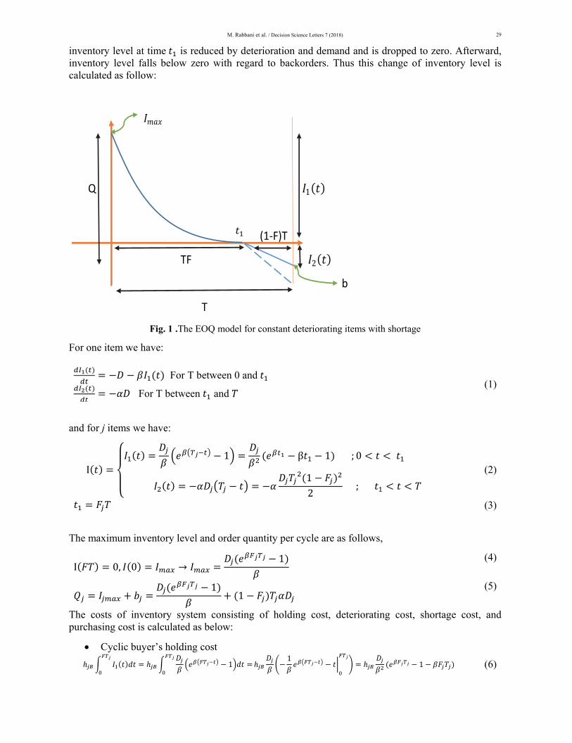
To calculate the cost of inventory system, at the first stage, we must calculate the inventory level. According to Fig. 1 demonstrating EOQ model for constant deteriorating items with shortage, the

M. Rabbani et al. / Decision Science Letters 7 (2018)

29

inventory level at time is reduced by deterioration and demand and is dropped to zero. Afterward, inventory level falls below zero with regard to backorders. Thus this change of inventory level is calculated as follow:

 

Fig. 1 .The EOQ model for constant deteriorating items with shortage

For one item we have:

For T between 0 and

For T between and (1)

and for j items we have:

I1 β 1 ; 0

12

;

(2)

(3)   

The maximum inventory level and order quantity per cycle are as follows,

I 0, 0 →1

(4)

11

(5)

The costs of inventory system consisting of holding cost, deteriorating cost, shortage cost, and purchasing cost is calculated as below: 

Cyclic buyer’s holding cost

11

1 (6)

                           

 

 

Q                                                                               1  

 

                                                                 (1‐F)T 

                                   TF                                             2  

                                                                                                b    

                                           T 

30

Cyclic deterioration cost

C1

(7)  

Cyclic shortage cost: π ∗ (8)

Cyclic purchasing cost 1

(9)

 As such, the total cost of buyer and supplier without considering VMI policy is as follows, respectively:

11

1 12

(10)

(11)

By considering Eq. (10) and Eq. (11), the total cost of inventory system without VMI policy is calculated as follow:

= ∑ 1

        (12)

 

3.1.2. Considering VMI policy

Now, we investigate a situation in which VMI policy is considered. In this policy, supplier should pay the buyer’s cost, therefore we have:

0  (13)   

The total cost function will be calculated as follows,

1 1 1

12

(14)

Since the average inventory of the j-th item is equal to ( ), the space constraint will be as follow:

∀ (15)

Also, the constraints for the bounds on the time period and budget for each item are as follows,

  (16)

  (17)

M. Rabbani et al. / Decision Science Letters 7 (2018)

31

The maximum backorder level of item j in a cycle must be less than or equal to its order quantity i.e.

(18) , 0 1,2, … ,  

0 1,2, … ,  

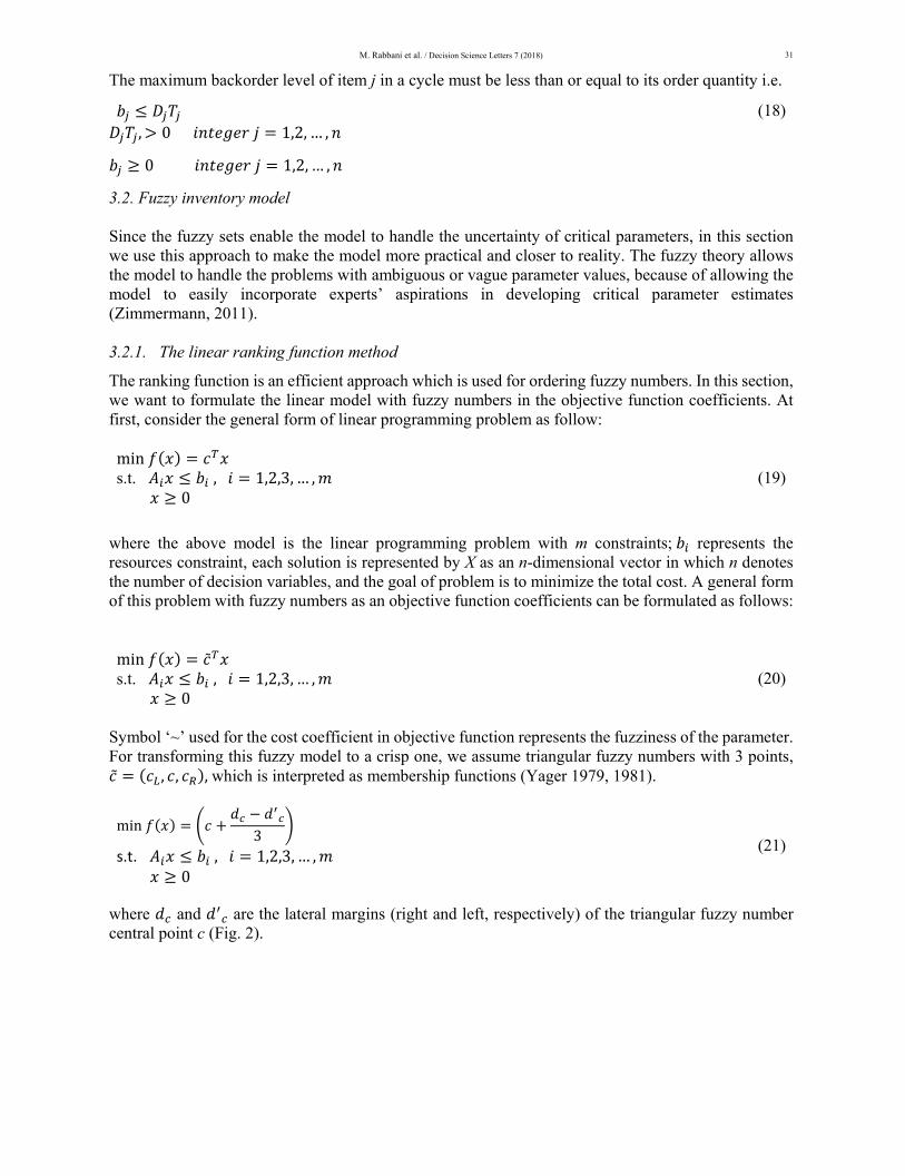
3.2. Fuzzy inventory model Since the fuzzy sets enable the model to handle the uncertainty of critical parameters, in this section we use this approach to make the model more practical and closer to reality. The fuzzy theory allows the model to handle the problems with ambiguous or vague parameter values, because of allowing the model to easily incorporate experts’ aspirations in developing critical parameter estimates (Zimmermann, 2011).

3.2.1. The linear ranking function method

The ranking function is an efficient approach which is used for ordering fuzzy numbers. In this section, we want to formulate the linear model with fuzzy numbers in the objective function coefficients. At first, consider the general form of linear programming problem as follow: min s.t. , 1,2,3, … , 0

(19)

where the above model is the linear programming problem with m constraints; represents the resources constraint, each solution is represented by X as an n-dimensional vector in which n denotes the number of decision variables, and the goal of problem is to minimize the total cost. A general form of this problem with fuzzy numbers as an objective function coefficients can be formulated as follows: min ̃ s.t. , 1,2,3, … , 0

(20)

Symbol ‘~’ used for the cost coefficient in objective function represents the fuzziness of the parameter. For transforming this fuzzy model to a crisp one, we assume triangular fuzzy numbers with 3 points, ̃ , , ,which is interpreted as membership functions (Yager 1979, 1981).

min3

 

s.t. , 1,2,3, … , 0 

(21)

where and are the lateral margins (right and left, respectively) of the triangular fuzzy number central point c (Fig. 2).

32

 

Fig. 2. Triangular fuzzy number

Fig. 3. Fuzzy resource with tolerance

3.2.2. Zimmerman method When we consider some tolerance for constraint resources, the problem with fuzzy resources should be formulated as follows (Zimmermann, 1976, 1985): min s.t. , 1,2,3, … , 0

(22)

In addition, let the membership functions of the fuzzy sets representing the fuzzy constraints be defined as:

1

1,2,3, … ,

0

(23)

where is the tolerance of problem resources (Fig. 3). The membership function of the objective function can be determined by solving the following two models:

1

1

M. Rabbani et al. / Decision Science Letters 7 (2018)

33

min s.t. , 1,2,3, … , 0

(24)

min s.t. , 1,2,3, … , 0

(25)

where the minimum total cost, , in the model with and without tolerance for resources is and , respectively. The membership function of the objective function is therefore as follows,

1

0

(26)

Using the settings in Eq. (26), the fuzzy problem is transformed into a crisp nonlinear programming problem as:

max s.t. 1

1 1,2,3, … , 0,0 1

(27)

where is the investment target, i.e., aspiration level of the objective function.

3.3.The proposed fuzzy model

Here, we propose a fuzzy model in which the demand and available space are fuzzy numbers.

min1 1 1

12

subject to ∀      

  ∀      

∀  

∀                                                     

, 0 1,2, … ,  

0 1,2, … ,  

(28)

Following Yager (1979, 1981) method for demand defuzzification and based on Zimmermann (1976, 1985) method for resource defuzzification, the fuzzy model is converted to:

max  s.t

1 /3 1

/31 /3 1

2

1

(29)

34

/3 1 ∀      

/ /∀      

/3 ∀  

/3 ∀                                           

     

/3 , 0 1,2,… ,  

0 1,2, … ,  

where is tolerances of respectively and is the investment target, i.e., aspiration level of the objective function.

4. Numerical Example

In order to demonstrate the application of the proposed procedure and to investigate its performances, five numerical examples are derived from the SAPCO Company which is an Iranian automobile supply company with different number of items (4, 8, 12, 16, and 20 items). The initial data of all test problems are shown in Table 1. Then, we compare the given results of two used approaches (SA, TS) in Tables 2 and Table 3.

Table 1 Initial data of the examples

item(j)

1 736 796 868 400 50 12 1 150 0.2 0.12 500 100 240 50 100 2 1236 1296 1368 400 50 12 1 150 0.2 0.12 500 120 260 50 100 3 1736 1796 1868 400 50 12 1 150 0.2 0.12 500 100 240 50 100 4 2236 2296 2368 400 50 12 1 150 0.2 0.12 500 120 264 50 100 5 2736 2796 2868 400 50 12 1 150 0.2 0.12 500 100 240 50 100 6 3236 3296 3368 600 70 6 0.5 200 0.25 0.08 700 120 240 50 132 7 3736 3796 3868 600 70 6 0.5 200 0.25 0.08 700 100 260 50 132 8 4236 4296 4368 600 70 6 0.5 200 0.25 0.08 700 120 240 50 132 9 4736 4796 4868 600 70 6 0.5 200 0.25 0.08 700 100 264 50 132 10 5236 5296 5368 600 70 6 0.5 200 0.25 0.08 700 120 240 50 132 11 736 796 868 400 50 12 1 150 0.2 0.12 500 100 240 50 100 12 1236 1296 1368 400 50 12 1 150 0.2 0.12 500 120 260 50 100 13 1736 1796 1868 400 50 12 1 150 0.2 0.12 500 100 240 50 100 14 2236 2296 2368 400 50 12 1 150 0.2 0.12 500 120 264 50 100 15 2736 2796 2868 400 50 12 1 150 0.2 0.12 500 100 240 50 100 16 3236 3296 3368 600 70 6 0.5 200 0.25 0.08 700 120 240 50 132 17 3736 3796 3868 600 70 6 0.5 200 0.25 0.08 700 100 260 50 132 18 4236 4296 4368 600 70 6 0.5 200 0.25 0.08 700 120 240 50 132 19 4736 4796 4868 600 70 6 0.5 200 0.25 0.08 700 100 264 50 132 20 5236 5296 5368 600 70 6 0.5 200 0.25 0.08 700 120 240 50 132

Table 2 The crisp total VMI cost obtained by the algorithms

Problem no. Number of items Objective Function Value (TC) The better

algorithm Improvement %

Simulated Annealing (SA) Tabu Search (TS) 1 4 8,276,300,000 8,276,300,000 The same 0 2 8 8,332,100,000 8,345,600,000 SA 0.16 3 12 8,415,200,000 8,415,400,000 SA 0.0023 4 16 8,484,100,000 8,497,300,000 SA 0.15 5 20 8,544,800,000 8,543,800,000 TS 0.011

 

Table 2 represents the crisp objective function value of each example which are calculated by two metaheuristic approaches (SA, TS). Moreover, computational time which is needed to tackle the problem are reported for both algorithms under different situations in Tables 4 and 5.

M. Rabbani et al. / Decision Science Letters 7 (2018)

35

Table 3 The Fuzzy total VMI cost obtained by the algorithms

Problem no. Number of items Objective Function Value (TC) The better

algorithm Improvement %

Simulated Annealing (SA) Tabu Search (TS) 1 4 8,215,200,000 8,274,600,000 SA 0.717 2 8 8,273,300,000 8,313,100,000 SA 0.478 3 12 8,360,400,000 8,361,200,000 SA 0.0095 4 16 8,413,900,000 8,427,100,000 SA 0.15 5 20 8,521,500,000 8,466,100,000 TS 0.65

 

Table 4 The required CPU time of the algorithms in crisp mode

Problem no. Number of items CPU Time The better algorithm Improvement% Simulated Annealing (SA) Tabu Search (TS)

1 4 0.560355 0.067039 TS 89.28 2 8 0.979735 0.433081 TS 55.67 3 12 1. 434864 0.540218 TS 62.23 4 16 1. 720567 0.774084 TS 55.23 5 20 2. 143143 0.929065 TS 57

Table 5 The required CPU time of the algorithms in fuzzy mode

Problem no. Number of items

CPU Time The better algorithm Improvement%

Simulated Annealing (SA) Tabu Search (TS) 1 4 0. 639240 0.205656 TS 67.82 2 8 1.206032 0.423702 TS 65 3 12 1. 617912 0.653496 TS 59.62 4 16 2. 048862 0.782272 TS 61.76 5 20 2. 572331 0.924853 TS 64.20

Table 6 The initial parameter values for the algorithms

Simulated Annealing(SA) Tabu Search (heist temperature) STM Size = 5

(coolest temperature ) LTM size = Number of items per problem R=0.98 (decreasing rate) Frequency = 1000 Maximum number of iteration per cycle = 20 Maximum number of accepted neighborhood per cycle = 15

5. Sensitivity Analysis

In this section, we analyze the effect of different parameters of the algorithms on optimal solution. Furthermore, we compare SA and TS based on the optimal solution as well as the CPU time.

5.1.Simulated Annealing (SA)

Fig. 4 demonstrates that the highest temperature in SA algorithm can influence on the optimal solution. In addition, the results of Fig. 5 show that the increase in temperature could increase the CPU time.

Fig. 4 . The effect of highest temperature on the objective value

Fig. 5. The effect of highest temperature on the CPU time

0

0.5

1

1.5

2

2.5

3

20 40 60 80 100

CPU tim

e

Temperature

8.4

8.5

8.6

8.7

8.8

8.9

20 40 60 80 100

oBJECTIVE 

TEMPERATURE

36

Moreover, the results of Fig. 6 and Fig. 7 demonstrate the effect of the coolest temperature on the objective function and the CPU time. As we can see from the figures, any increase on temperature also increases the objective function by reduces the Cpu time.

Fig. 6 .The effect of the coolest temperature on the objective value

Fig. 7.The effect of the coolest temperature on the CPU time

5.2.Tabu Search

Fig. 10 and Fig. 11 show the effects of STM size on the CPU time and the objective function, respectively. As we can observe from the results, while any increase on STM reduces the CPU time it has no significant impact on the objective finction.

Fig. 8 .The effect of STM size on the CPU time Fig. 9 .The effect of STM size on the objective value

6. Conclusion

In this study, we have considered a multi-item multi-constraint economic order quantity (EOQ) model which is concerned with some assumptions such as deterioration, Vendor Manage Inventory (VMI) strategy, shortage in form of partial backorder, and also some constraints such as available storage space, limited time period of cycle and limited total budget for purchasing goods to make the model more practical.  In order to determine the impact of VMI on the objective function value, we have considered the before and after strategies, separately. In addition to the conditions listed above, we have considered the model in form of fuzzy to enable the model to handle the uncertainty of critical parameters and compared the crisp and fuzzy results of five numerical examples derived from the SAPCO Company with different number of items (4, 8, 12, 16, and 20 items) which is for demonstrating the application of the proposed procedure and to investigate its performances, obtained by two

8.4

8.45

8.5

8.55

8.6

8.65

8.7

0 20 40 60 80

Objective value

Temperature

0

0.5

1

1.5

2

2.5

3

‐10 10 30 50 70

CPU tim

e

Temperature

0.34

0.35

0.36

0.37

0.38

0.39

‐5 15 35 55

CPU tim

e

STM size

7.5

8

8.5

9

9.5

0 20 40 60

Objective value

STM size

M. Rabbani et al. / Decision Science Letters 7 (2018)

37

metaheuristic approaches, Simulated Annealing (SA) and Tabu Search (TS). For improving the solving time of algorithm, we have used some approximation using the Taylor series expansion as an initial solution. Furthermore, the most sensitive parameters of the proposed methodology were identified by carrying out the sensitivity analysis. The analysis has indicated that by using the approximation of the Taylor series expansion, the efficiency of the algorithms was increased because the initial solution was close enough to a good solution and it could help the algorithm find a good solution rapidly.

For future research, some interested issues are suggested as follow:

Due to the backorder, completely backordered and also lost sales can be considered for shortage. The deterioration rate can be assumed as a variable rate. Instead of constant rate of demand, a variable or stochastic rate can be investigated. The EOQ model can also be considered as an EPQ model. Other constraints such as limitations on buyer's total order quantity of the items, limitation on

the number of pallets for an items can be also taken into account.

References

Abad, P. L. (2001). Optimal price and order size for a reseller under partial backordering. Computers & Operations Research, 28(1), 53-65.

Bahari-Kashani, H. (1989). Replenishment schedule for deteriorating items with time-proportional demand. Journal of the operational research society, 40(1), 75-81.

Bhunia, A. K., & Maiti, M. (1998). Deterministic inventory model for deteriorating items with finite rate of replenishment dependent on inventory level. Computers & operations research, 25(11), 997-1006.

Cárdenas-Barrón, L. E., Treviño-Garza, G., & Wee, H. M. (2012). A simple and better algorithm to solve the vendor managed inventory control system of multi-product multi-constraint economic order quantity model. Expert Systems with Applications, 39(3), 3888-3895.

Covert, R. P., & Philip, G. C. (1973). An EOQ model for items with Weibull distribution deterioration. AIIE transactions, 5(4), 323-326.

Farrokhi-Asl, H., Tavakkoli-Moghaddam, R., Asgarian, B., & Sangari, E. (2016). Metaheuristics for a bi-objective location-routing-problem in waste collection management. Journal of Industrial and Production Engineering, 1-14.

Ghare, P. M., & Schrader, G. F. (1963). A model for exponentially decaying inventory. Journal of industrial Engineering, 14(5), 238-243.

Goswami, A., & Chaudhuri, K. S. (1991). An EOQ model for deteriorating items with shortages and a linear trend in demand. Journal of the Operational Research Society, 42(12), 1105-1110.

Guchhait, P., Maiti, M. K., & Maiti, M. (2015). An EOQ model of deteriorating item in imprecise environment with dynamic deterioration and credit linked demand. Applied Mathematical Modelling, 39(21), 6553-6567.

Hall, R. W., & American Production and Inventory Control Society. (1983).Zero inventories. Homewood, IL: Dow Jones-Irwin.

Harris, F. W. (1913). How many parts to make at once. Factory, the Magazine of Management, 10(2), 135-136.

Herron, D. P. (1979). Managing physical distribution for profit. Harvard Business Review, 57(3), 121-132.

Kazemi, N., Olugu, E. U., Abdul-Rashid, S. H., & Ghazilla, R. A. R. (2016). A fuzzy EOQ model with backorders and forgetting effect on fuzzy parameters: An empirical study. Computers & Industrial Engineering, 96, 140-148.

Maity, K., & Maiti, M. (2009). Optimal inventory policies for deteriorating complementary and substitute items. International Journal of Systems Science, 40(3), 267-276.

38

Ouyang, L. Y., Teng, J. T., Goyal, S. K., & Yang, C. T. (2009). An economic order quantity model for deteriorating items with partially permissible delay in payments linked to order quantity. European Journal of Operational Research, 194(2), 418-431.

Park, K. S. (1983). An integrated production-inventory model for decaying raw materials. International Journal of Systems Science, 14(7), 801-806.

Poozesh, P., Baqersad, J., Niezrecki, C., Harvey, E., & Yarala, R. (2014). Full field inspection of a utility scale wind turbine blade using digital image correlation. CAMX, Orlando, FL, 10(2.1), 2891-2960.

Rabbani, M., Ramezankhani, M. J., Farrokhi-Asl, H., & Farshbaf-Geranmayeh, A. (2015). Vehicle Routing with Time Windows and Customer Selection for Perishable Goods. International Journal of Supply and Operations Management, 2(2), 700-719.

Sana, S. S. (2010). Optimal selling price and lot size with time varying deterioration and partial backlogging. Applied Mathematics and Computation, 217(1), 185-194.

Tadikamalla, P. R. (1978). An EOQ inventory model for items with gamma distributed deterioration. AIIE transactions, 10(1), 100-103.

Tai, A. H., Xie, Y., & Ching, W. K. (2016). Inspection policy for inventory system with deteriorating products. International Journal of Production Economics, 173, 22-29.

Tat, R., Taleizadeh, A. A., & Esmaeili, M. (2015). Developing economic order quantity model for non-instantaneous deteriorating items in vendor-managed inventory (VMI) system. International Journal of Systems Science, 46(7), 1257-1268.

Waller, M., Johnson, M. E., & Davis, T. (1999). Vendor-managed inventory in the retail supply chain. Journal of business logistics, 20(1), 183.

Whitin, T.M. (1957).Theory of inventory management. Princeton, NJ: Princeton University Press. Wee, H. M., & Law, S. T. (2001). Replenishment and pricing policy for deteriorating items taking into

account the time-value of money. International Journal of Production Economics, 71(1), 213-220. Wee, H. M., Lo, C. C., & Hsu, P. H. (2009). A multi-objective joint replenishment inventory model

of deteriorated items in a fuzzy environment. European Journal of Operational Research, 197(2), 620-631.

Wu, J., Ouyang, L. Y., Cárdenas-Barrón, L. E., & Goyal, S. K. (2014). Optimal credit period and lot size for deteriorating items with expiration dates under two-level trade credit financing. European Journal of Operational Research, 237(3), 898-908.

Yager, R. R. (1979, January). Ranking fuzzy subsets over the unit interval. In Decision and Control including the 17th Symposium on Adaptive Processes, 1978 IEEE Conference on (pp. 1435-1437). IEEE.

Yager, R. R. (1981). A procedure for ordering fuzzy subsets of the unit interval. Information Sciences, 24(2), 143-161.

Yu, Y., & Huang, G. Q. (2010). Nash game model for optimizing market strategies, configuration of platform products in a Vendor Managed Inventory (VMI) supply chain for a product family. European Journal of Operational Research, 206(2), 361-373.

Yu, Y., Chu, C., Chen, H., & Chu, F. (2012). Large scale stochastic inventory routing problems with split delivery and service level constraints. Annals of Operations Research, 197(1), 135-158.

Zanoni, S., & Zavanella, L. (2007). Single-vendor single-buyer with integrated transport-inventory system: Models and heuristics in the case of perishable goods. Computers & Industrial Engineering, 52(1), 107-123.

© 2018 by the authors; licensee Growing Science, Canada. This is an open access article distributed under the terms and conditions of the Creative Commons Attribution (CC-BY) license (http://creativecommons.org/licenses/by/4.0/).