Velocity Kinematics and Static Force Analysis

Up to this point we have considered only static positioning problems for a robotic manipulator. We nowstart to introduce the idea of motion into our analysis.

As a first step we consider the problem of deriving the velocity of the end effector for some arbitrarymanipulator

To do this we will need a thorough understanding kinematic velocity analysis, and the tools involved:frames, moving frames, time derivatives of vectors, linear and angular velocities and their different rep-resentations.

What will turn out to be important is the relationship between the velocity in Cartesian space of the endeffector and the velocity of the robot configuration in joint space.

The Jacobian, a matrix of derivatives, will be introduced as the key representation of this relationship

It will turn out that we can also achieve a static force/torque analysis of the manipulator using theJacobian, and we will also explore this idea.

Structure of this Section

Thus the structure of the following lecture notes is:

• velocity of a single point

• velocity of a rigid body

• velocity analysis of a robotic manipulator

• the Jacobian

• Singularities

• Static Force Analysis

Velocity of a Point in Space

Consider the a vector Q expressed in frame B, ie BQ, that represents the position of a particle in space.

Then the velocity of of that particle, BVQ, can be determined by taking the time derivative:

1

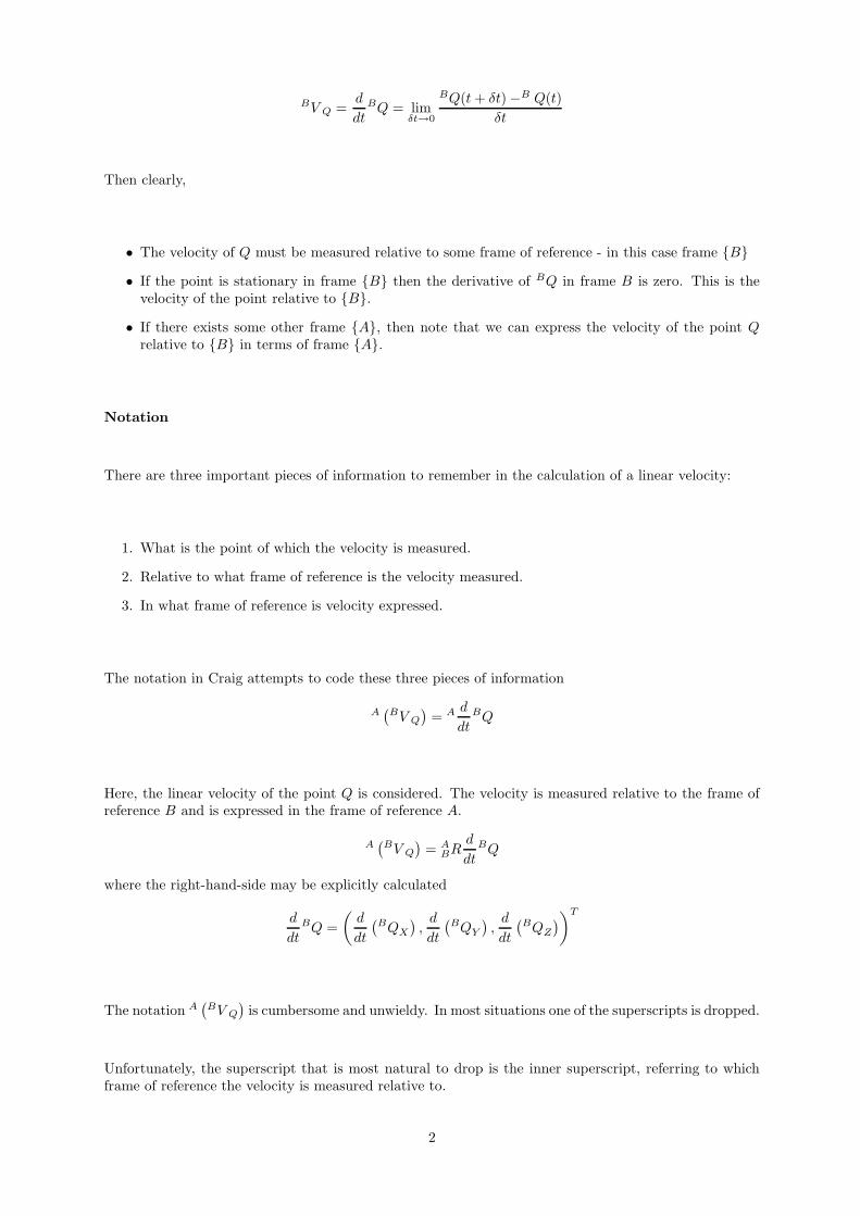
BV Q =d

dtBQ = lim

δt→0

BQ(t+ δt) −B Q(t)

δt

Then clearly,

• The velocity of Q must be measured relative to some frame of reference - in this case frame B

• If the point is stationary in frame B then the derivative of BQ in frame B is zero. This is thevelocity of the point relative to B.

• If there exists some other frame A, then note that we can express the velocity of the point Qrelative to B in terms of frame A.

Notation

There are three important pieces of information to remember in the calculation of a linear velocity:

1. What is the point of which the velocity is measured.

2. Relative to what frame of reference is the velocity measured.

3. In what frame of reference is velocity expressed.

The notation in Craig attempts to code these three pieces of information

A(

BV Q)

= A d

dtBQ

Here, the linear velocity of the point Q is considered. The velocity is measured relative to the frame ofreference B and is expressed in the frame of reference A.

A(

BV Q)

= ABR

d

dtBQ

where the right-hand-side may be explicitly calculated

d

dtBQ =

(

d

dt

(

BQX)

,d

dt

(

BQY)

,d

dt

(

BQZ)

)T

The notation A(

BV Q)

is cumbersome and unwieldy. In most situations one of the superscripts is dropped.

Unfortunately, the superscript that is most natural to drop is the inner superscript, referring to whichframe of reference the velocity is measured relative to.

2

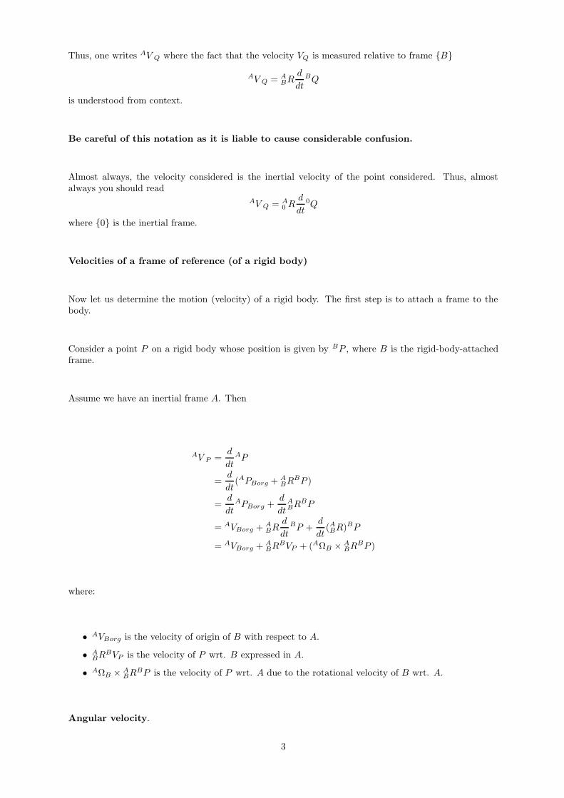
Thus, one writes AV Q where the fact that the velocity VQ is measured relative to frame B

AV Q = ABR

d

dtBQ

is understood from context.

Be careful of this notation as it is liable to cause considerable confusion.

Almost always, the velocity considered is the inertial velocity of the point considered. Thus, almostalways you should read

AV Q = A0 R

d

dt0Q

where 0 is the inertial frame.

Velocities of a frame of reference (of a rigid body)

Now let us determine the motion (velocity) of a rigid body. The first step is to attach a frame to thebody.

Consider a point P on a rigid body whose position is given by BP , where B is the rigid-body-attachedframe.

Assume we have an inertial frame A. Then

AV P =d

dtAP

=d

dt(APBorg + A

BRBP )

=d

dtAPBorg +

d

dtABR

BP

= AVBorg + ABR

d

dtBP +

d

dt(ABR)BP

= AVBorg + ABR

BVP + (AΩB × ABR

BP )

where:

• AVBorg is the velocity of origin of B with respect to A.

• ABR

BVP is the velocity of P wrt. B expressed in A.

• AΩB × ABR

BP is the velocity of P wrt. A due to the rotational velocity of B wrt. A.

Angular velocity.

3

We have introduced AΩB , but what is it?

AΩB is the angular velocity of a frame B with respect to a frame of reference A. It can be representedby a triple of numbers:

AΩB = [Ω1,Ω2,Ω3]T

Its direction represents the instantaneous axis of rotation of frame B with respect to a frame A,while its magnitude represents the speed of this rotation.

AΩB is obviously related to the derivative of the rotation matrix BAR, and we shall explore this relationship

later.

An additional point is that, like any other vector, we can express AΩB wrt. some other frame, say U ,giving the cumbersome notation by Craig of

U (AΩB)

where U is some absolute inertial frame, which leads to Craig introducing the notation

ωB =U ΩB

when the identity of this absolute reference frame is clear.

We have also introduced the cross product in the final term of the equation on the previous slide forAV P , and we shall explore why we do this later.

Special Cases

First, lets check the special cases of rigid body motion:

• When B is purely translating with respect to A, AΩB × ABR

BP = 0 since AΩB = 0. Hence

AV P = AVBorg + ABR

BVP

4

• When B is purely rotating with respect to A, then AVBorg = 0, and

AV P = ABR

BVP + (AΩB × ABR

BP )

• When P is fixed with respect to B (usually the case if P is point on rigid body), then ABR

BVP = 0,and

AV P = AVBorg + (AΩB × ABR

BP )

Summary

We can summarise the results so far as:

• The velocity of a point P is calculated as the time derivative of the position of P .

• This derivative must be taken with respect to some frame, say frame B, giving BVP

• The velocity vector can be express in terms of another frame, say A, so that we can have A(BVP ).

• When a point P is expressed in some frame B, and we wish to calculate its velocity (ie. take thederivative) with respect to some other frame A, then we get

AV P = AVBorg + ABR

BVP + (AΩB × ABR

BP )

• This equation shows that AV P derives from three things

– the linear velocity of P wrt. the origin of B

– the linear velocity of the origin of B wrt. the origin of A

– the rotational velocity of B wrt. A

• the rotational velocity of B wrt. A is given by the angular velocity Ω, which represents both anaxis and magnitude of rotation.

In the following slides we will focus in on the AΩB × ABR

BP term. We have introduced this term, butnot really explained where it has come from. But first and example.

Example 5.1:

Skew symmetric matrices and the derivative of R

Rotation matrices are elements of the group of orthogonal matrices

SO(3) = R ∈ <3×3 RTR = I3, det(R) = 1

For the case where a frame, say B, is rotating with respect to another, say A, we are interested in acontinuous dynamic change in a rotation matrix.

5

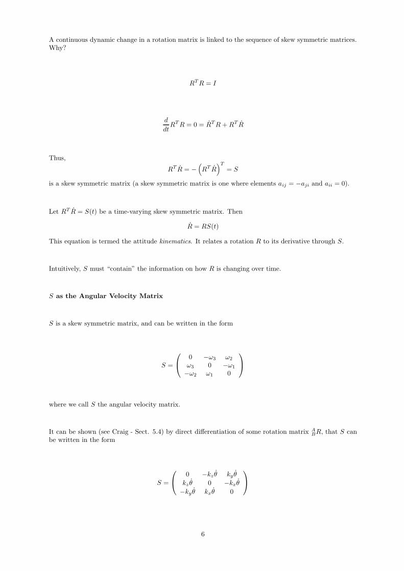
A continuous dynamic change in a rotation matrix is linked to the sequence of skew symmetric matrices.Why?

RTR = I

d

dtRTR = 0 = RTR+RT R

Thus,

RT R = −(

RT R)T

= S

is a skew symmetric matrix (a skew symmetric matrix is one where elements aij = −aji and aii = 0).

Let RT R = S(t) be a time-varying skew symmetric matrix. Then

R = RS(t)

This equation is termed the attitude kinematics. It relates a rotation R to its derivative through S.

Intuitively, S must “contain” the information on how R is changing over time.

S as the Angular Velocity Matrix

S is a skew symmetric matrix, and can be written in the form

S =

0 −ω3 ω2

ω3 0 −ω1

−ω2 ω1 0

where we call S the angular velocity matrix.

It can be shown (see Craig - Sect. 5.4) by direct differentiation of some rotation matrix ABR, that S can

be written in the form

S =

0 −kz θ ky θ

kz θ 0 −kxθ

−ky θ kxθ 0

6

where K = [kx, ky, kz ]T is the unit vector passing though the origin of A and B with a line of action

defining the axis of rotation and where θ gives the magnitude of the rotational velocity.

So S does define the rotational velocity of frame B wrt. A.

The Angular Velocity Vector Ω

We are interested in deriving the expression AΩB × ABR

BP . Recall this was the component of AV due tothe rotation of frame B wrt. A.

If we take the derivative of

AV P =d

dtAP

=d

dt(APBorg + A

BRBP )

=d

dtAPBorg +

d

dtABR

BP

= AVBorg + ABR

d

dtBP +

d

dt(ABR)BP

= AVBorg + ABR

BVP +d

dt(ABR)ABR

−1AP

= AVBorg + ABR

BVP + SAP

= AVBorg + ABR

BVP + (AΩB × AP )

= AVBorg + ABR

BVP + (AΩB × ABR

BP )

Where did Ω come from?

Where did the cross product come from?

A well known property of a skew symmetric matrix is that, if

S =

0 −ω3 ω2

ω3 0 −ω1

−ω2 ω1 0

and

Ω = [ω1, ω2, ω3]T

7

then, for some vector AP ,

SAP = Ω × AP

where we have seen previously that Ω, say AΩB , is the angular velocity vector which has a directionrepresenting the instantaneous axis of rotation of frame B with respect to a frame A, and a magnituderepresenting the speed of this rotation.

Wedge Product

Any skew symmetric matrix Ω (in <3×3) may be written

Ω =

0 −ω3 ω2

ω3 0 −ω1

−ω2 ω1 0

Thus, Ω is parameterised by three components

ω =

ω1

ω2

ω3

NotationΩ = ω∧

Note that

ω × v =

ω2v3 − v2ω3

ω2v1 − ω1v3ω1v2 − ω2v1

=

0 −ω3 ω2

ω3 0 −ω1

−ω2 ω1 0

v = ω∧v

The skew parameterisation ω∧ is equivalent to the matrix representation of the linear op-erator associated with the vector cross product.

So you may see AVP written alternatively as:

AV P = AVBorg + ABR

BVP + (AΩB ∧ ABR

BP )

Attitude Kinematics Revisited.

8

Recall the attitude kinematicsd

dtABR = A

BRS(t)

obtained by differentiating RTR = I3.

Note that one could also differentiate RRT = I3 to obtain a relation

d

dtABR = S(t)ABR

This leads to a relationshipABRS(t)ABR

T= S(t)

• S relates the angular velocity of frame B with respect to frame A written with respect to frameB.

• Conversely, S relates the angular velocity of frame B with respect tot frame A written withrespect to frame A.

Alternative representations to “Angle-axis” approach: Euler angles

The attitude kinematics may also be expressed in terms of the other representations.

Consider the Z-Y-X Euler anglesABR := RφRθRψ

The angular velocity of B with respect to A, expressed in frame A is the sum of the componentsdue to the rotation of each individual Euler angle

AΩB = φe3 + θRφe2 + ψRφRθe1.

• The first term is associated with the rotation φ taken around the ZA ∈ A axis, where ZA is justthe e3 co-ordinate vector.

• The θ rotation occurs around Rφe2 the rotated version of Y1. The Y axis of the rotated frame afterthe yaw rotation has been applied.

• Finally the roll ψ occurs around the axis RφRθe1, the image of XA under the first two rotations

Computing these rotations yields

AΩB = φ

001

+ θ

−sφcφ0

+ ψ

cθcφcθsφsθ

=

0 −sφ cθcφ0 cφ cθsφ1 0 −sθ

φ

θ

ψ

= W (φ, θ, ψ)

φ

θ

ψ

9

From the above we have

φ

θ

ψ

= W−1(φ, θ, ψ)AΩB .

This equation is termed the attitude kinematics for the Z-Y-X Euler angles. It denotes the rateof change of the Euler angles given a known angular velocity.

The inverse of BW is given by

BW−1

:=1

cos(θ)

0 sψ cψ0 cθcψ −cθsψcθ sθsψ sθcψ

.

Note thatdet(W ) = − cos(θ)

and thus the Euler angle attitude kinematics are not valid where θ = π2 . This singularity is related to

the non-uniqueness of the Euler angle representation.

In the frame B the angular velocity is given by

Bω = BARW (φ, θ, ψ)

φ

θ

ψ

= BW (φ, θ, ψ)

φ

θ

ψ

where

BW (φ, θ, ψ) =

−sθ 0 1cθsψ cψ 0cθcψ −sψ 0

Velocity analysis of a manipulator

Now apply the velocity kinematic tools seen thus far to the specific case of a robotics manipulator.

In computing the velocity kinematics of manipulator the aim is to express the velocity of the end effectorwith respect to the station or base frame, which is a non-moving, or inertial frame.

The joint velocities θi or di will provide information about the velocity of the frame i with respect toframe i− 1.

In general, the velocity, d/dt0P comprises a component due to the inertial velocity of the base frame A(if it is non-zero), a component due to the velocity of B relative to A (rotational and linear) and thevelocity of BP .

10

In each case the actual velocity vector V of some point on the end effector is a vector that can be expressedin any of the frames of reference

AV P = ABR

BV P ,0V P = 0

ARABR

BV P

Note : in order to extend a kinematic model to a dynamic model, velocities must be measured relativeto some inertial frame of reference.

Although the velocity is the inertial velocity - it is often written in the local frame of reference.

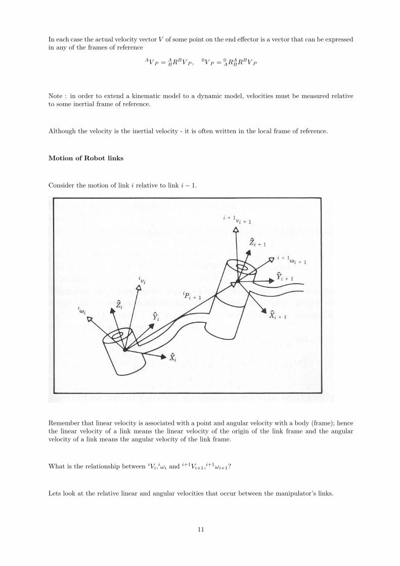
Motion of Robot links

Consider the motion of link i relative to link i− 1.

Remember that linear velocity is associated with a point and angular velocity with a body (frame); hencethe linear velocity of a link means the linear velocity of the origin of the link frame and the angularvelocity of a link means the angular velocity of the link frame.

What is the relationship between iVi,iωi and i+1Vi+1,

i+1ωi+1?

Lets look at the relative linear and angular velocities that occur between the manipulator’s links.

11

Relative Linear Velocity between Links

Consider the motion of link i relative to link i− 1.

The linear velocity of i is

i−1Vi =d

dti−1Pi =

d

dti−1i T (di, θi)

iPi

=d

dt

cθi−sθi

0 ai−1

sθicαi−1

cθicαi−1

−sαi−1−sαi−1

disθisαi−1

cθisαi−1

cαi−1cαi−1

di0 0 0 1

0001

=d

dt

ai−1

sαi−1di

cαi−1di

1

= di

1 0 0 00 cαi−1

−sαi−10

0 sαi−1cαi−1

00 0 0 1

0011

= diZi

where iPi is the position of the origin of frame i in frame i, and i−1i T (di, θi) is the link i − 1 to i

homogeneous transformation.

In retrospect this is no surprise since the point i−1P i is fixed for revolute joints and can only move in thejoint axis direction Zi for prismatic joints.

Relative Angular Velocity between Links

Using the geometric insights of above, the angular velocity of link i relative to link i− 1 is given by

i−1ωi = θii−1Zi

So, to summarise, for the two types of joint, either

i−1Vi = dii−1Zi, or i−1ωi = θi

i−1Zi.

The above expressions both relate the kinematic velocity of link i relative to link i− 1. In practice, onewishes to understand the inertial velocity of link i measured relative to the station frame.

Thus, the velocity of i should be calculated relative to 0.

Inertial linear velocity of link i

12

The inertial velocity of link i measured relative to an inertial frame can be derived from the relative linkvelocity (i−1Vi,

i−1ωi) and the inertial velocity(

0V i−1

)

of link i− 1.

Note that velocity components, either linear or angular, sum as long as they are expressed in the same

frame of reference.

A geometric argument gives

i−1(

0Vi)

=(

i−1ωi−1 ×i−1P i

)

+ i−1(

0Vi−1

)

+ dii−1Zi

• The term (i−1ωi ×i−1P i) is due to the point i−1P i rotating around the origin of the frame i− 1

with its angular velocity. Note that i−1ωi−1 is the angular velocity of frame i− 1 and need notlie in direction i−1Zi−1 since it is derived from all the previous rotation movements of the roboticmanipulator.

• The term i−1(

0Vi−1

)

is the linear velocity of frame i− 1.

• The term dii−1Zi is the linear velocity of frame i expressed in frame i− 1.

• One of either the first or third terms in this equation will be zero depending on whether the jointin question is prismatic or revolute.

To save notation we will write pvq = p(

0Vq)

to denote the inertial velocity of link q expressed in framep. Thus,

i−1vi =(

i−1ωi−1 ×i−1P i

)

+ i−1vi−1 + dii−1Zi

Inertial angular velocity of link i

Letpωq = p

(

0ωq)

denote the inertial angular velocity of link q expressed in frame p.

A geometric argument givesi−1ωi = i−1ωi−1 + θi

i−1Zi

This is a direct consequence of summation of angular velocities in frame i− 1.

Iterative solution for velocity of link i

We have seen that the inertial velocities of a link i can be expressed in terms of the inertial velocities oflink i− 1 and the relative velocities of link i wrt. link i− 1.

We are interested in determining the inertial velocity of the end effector, expressed in some frame, usuallythe frame attached to the base of the robot (which is usually inertial).

13

This suggests an iterative scheme where we iteratively propagate link velocities, starting from the robotbase, moving one link at a time until we reach the end effector link.

The velocity of link i relative to the inertial base frame 0 can be calculated iteratively as follows:

1. Set 0ω0 = 0 and 0v0 = 0. Thus, the initial reference frame is stationary. Set i = 0.

2. Increment i by one. (The index i takes the values i = 1, . . . , n). Compute the link i velocity inframe i− 1 according to the iterative equations,

i−1ωi = i−1ωi−1 + θii−1Zi

i−1vi = i−1vi−1 + (i−1ωi−1 ×i−1P i) + di

i−1Zi.

3. If i = n then set0ωn = 0

n−1Rn−1ωn,

0vn = 0n−1R

n−1vn.

Otherwise, transform the computed link velocity from frame i− 1 to frame i

iωi = ii−1R

i−1ωiivi = i

i−1Ri−1vi

and return to step 2).

Example 5.2:

Jacobians

In general a Jacobian is simply a matrix representation of a multi-dimensional derivative.

Let f1, f2, . . . fm each be a some differentiable functions mapping <1 → <m

y1 = f1(x1, x2, . . . , xn)y2 = f2(x1, x2, . . . , xn)

...ym = fm(x1, x2, . . . , xn)

Then we can write all the derivatives, ie. of each yi with respect to each xj , as a matrix

Jf (x) =

∂f1(x)∂x1

· · · ∂f1(x)∂xn

......

∂fm(x)∂x1

· · · ∂fn(x)∂xn

14

where x = x1, x2, . . . , xn, and where Jf (x) is called the Jacobian.

Velocity Jacobian of a Manipulator

Up to this point we have determined methods to derive the linear v and angular ω velocity of the robotend effector.

We have found that we derive expressions for v and w that include the joint angles/extensions q1, q2, .., qnand joint rates q1, q2, .., qn.

It turns out that we can write down these expressions in a general way as

v = Jp(q1, . . . qn)q

andω = Jo(q1, . . . qn)q

where, for a 6-dof manipulator (n = 6):

• v is the (3x1) vector of linear velocities in the x,y and z directions.

• w is the (3x1) vector of angular velocities around the x,y and z directions.

• q = [q1, q2, .., q6]T , the vector of joint velocities.

• Jp is a jacobian; a (3x6) matrix governing the contribution of joint velocities q to the end effectorlinear velocity.

• Jo is also a jacobian; a (3x6) matrix governing the contribution of joint velocities q to the endeffector angular velocity.

The usual approach is to stack these Jacobians on top of one another to form the equation for theCartesian velocity V as:

V =

(

vω

)

= J(q1, . . . qn)q

where we denote

J =

(

JpJo

)

15

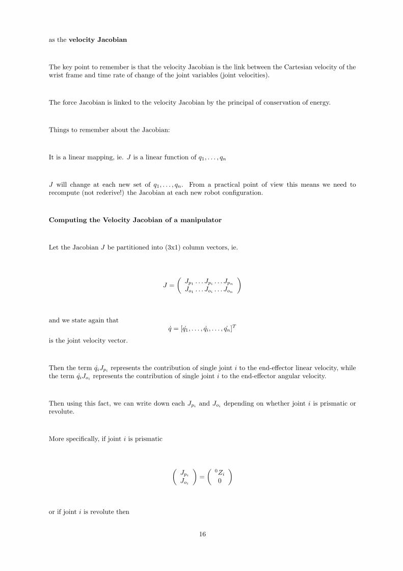
as the velocity Jacobian

The key point to remember is that the velocity Jacobian is the link between the Cartesian velocity of thewrist frame and time rate of change of the joint variables (joint velocities).

The force Jacobian is linked to the velocity Jacobian by the principal of conservation of energy.

Things to remember about the Jacobian:

It is a linear mapping, ie. J is a linear function of q1, . . . , qn

J will change at each new set of q1, . . . , qn. From a practical point of view this means we need torecompute (not rederive!) the Jacobian at each new robot configuration.

Computing the Velocity Jacobian of a manipulator

Let the Jacobian J be partitioned into (3x1) column vectors, ie.

J =

(

Jp1 . . . Jpi. . . Jpn

Jo1 . . . Joi. . . Jon

)

and we state again thatq = [q1, . . . , qi, . . . , qn]

T

is the joint velocity vector.

Then the term qiJpirepresents the contribution of single joint i to the end-effector linear velocity, while

the term qiJoirepresents the contribution of single joint i to the end-effector angular velocity.

Then using this fact, we can write down each Jpiand Joi

depending on whether joint i is prismatic orrevolute.

More specifically, if joint i is prismatic

(

Jpi

Joi

)

=

(

0Zi0

)

or if joint i is revolute then

16

(

Jpi

Joi

)

=

(

0Zi × (0p−0 pi)0Zi

)

0Zi is the unit vector along the joint axis of joint i expressed in the inertial frame.

0p is the position of the point we are interested in determining the velocity for (the end effector) and 0piis the position of the origin of the ith frame.

Note that given we have the forward kinematic transformations of a manipulator, ie. 0T1,0T2, . . .

0TN ,we can read off the values for 0p1,

0 p2, . . .0 p as the first three elements of the fourth columns of these

matrices respectively.

The above determination of the Jacobian was on the basis of geometric intuition.

It is also interesting to note that one can derive the Jacobian directly by differentiating the forwardkinematic equations with respect to the joint variables - but we will not do it here :-)

Frames of Reference and the Velocity Jacobians

The velocity Jacobian J(q) must be identified with a frame of reference in which the Cartesian velocityV finally expressed.

Up to this point we have assumed that the Jacobian is identified with the base frame 0, ie 0J(q).

It is possible that we may want to convert the Jacobian to be relevant to another frame, so that our endeffector Cartesian velocity calculations are output with respect to another frame (say the station frame).

First note that a frame transformation on a (6x1) Cartesian velocity vector may be achieved accordingto

(

AvAω

)

=

(

ABR 00 A

BR

)(

BvBω

)

so that

(

AvAω

)

=

(

ABR 00 A

BR

)

BJ(q)q

17

and so

AJ(q) =

(

ABR 00 A

BR

)

BJ(q)

Example 5.3:

The Jacobian and trajectory tracking

Consider a smooth trajectory a of a robot expressed in Cartesian coordinates of the end effector

a : t 7→ 0nT (t).

The velocity of the end effector isd

dt0nT (t) = 0

nV(t)

From the velocity Jacobian one has

0nV(t) =

(

0vn(t)0ωn(t)

)

= J(q)q

Thus, to track the desired trajectory it is sufficient to assign a speed controller to joints to achieve

q = J−1(q)

(

0ωn(t)0vn(t)

)

Hence, in robotics, we are most often interested in the inverse of the Jacobian.

Inverting the velocity Jacobian.

In a typical industrial manipulator there are exactly the same number of active joint variables as degreesof freedom.

For a full 6DOF manipulator moving in SE(3) then there are 6 active joint variables q = (q1, . . . , q6).

As a consequenceJ(q) ∈ <6×6

is a square matrix and

18

q = J−1(q)

(

0ωn(t)0vn(t)

)

= J−1(q)0Vn(t)

is defined as long as J(q) is invertible.

Dealing with under-actuated manipulators.

If there are insufficient joints actuated, say p < 6 joints, to achieve full 6DOF movement the situationbecomes somewhat more serious.

In this caseJ(q) ∈ <p×6

is rank p.

To solve the tracking problem one requires that 0Vn(t) lies in the range space of J(q) in order that

J(q)q = 0Vn(t)

has a solution q.

The range space of J(q) = spancolJ(q) is the subspace of accessible velocities for the manipulator. Itis associated with tangent direction to the manipulator subspace for an under-actuated manipulator.

If the velocity profile desired is derived from differentiating a smooth curve in the forward kinematics(one that satisfies the manipulator subspace constraints) then the velocity constraint is automaticallysatisfied.

Singularities

Even in the case where there are 6 joints for 6DOF robotic manipulator there can be problems in solving

q = J−1(q)0Vn(t)

This equation cannot be solved if J(q) becomes singular. That is, if the range space of J(q) degeneratesin at least one direction. Denote the degenerate direction of J(q) at a singular point by v, then

vTJ(q)q = 0 = vT 0Vn(t)

for all q. Thus, 0Vn(t) must be orthogonal to v. Such points are called singularities of the mechanism.

Singularities are a fundamental part of an actuator mechanism.

19

1. They represent configurations at which the mobility of the mechanism is reduced, ie. it is notpossible to impose an arbitrary motion on the end effector.

2. In the neighbourhood of a singularity, small velocities in the operational space may cause largevelocities in the joint space.

Types of Singularities

1. Workspace boundary singularities: It is clear that the end link of a manipulator cannot bemoved beyond the boundary of its workspace. All boundary points must be singular points of themanipulator. The singular direction v is the normal to the workspace boundary.

2. Workspace interior singularities: Singularities are also possible within the workspace. Theyare usually due to the alignment of two or more joint axes eg. when joint axis 5 on Puma is zero.

Example 5.4:

Locating the singularities of a manipulator

To locate all the singularities of a manipulator

1. Use your physical insight of the manipulator geometry and workspace to identify workspace bound-ary singularities and interior point singularities.

2. Compute the determinant of the velocity Jacobian and find q such that

det (J(q)) = 0

This equation leads to complicated non-linear equations in q that often cannot be solved in closed-form. This approach can be used for simple manipulators but is most often used as confirmationof singularity rather than a means to find singular points.

Trajectory tracking in the vicinity of singularities

Consider a 6DOF manipulator moving within its workspace in SE(3). Let 0Vn(t) be a bounded velocityprofile of a trajectory that passes close to a singularity but does not pass through the singularity.

Thus,∣

∣

0Vn(t)∣

∣ < B0

for some bound B0 > 0 anddet (J(q)) > ε

for ε > 0. Note that ε may be small.

20

The joint velocities for trajectory tracking are well defined at all points on the trajectory.

q = J−1(q)0Vn(t)

Due to the inverse in the Jacobian the best general bound on the joint velocities that is possible is

|q| ≤B0

ε

The potentially large values of q generated by the trajectory tracking algorithm may easily violate thejoint motor capabilities. This is a natural consequence of operating close the structural limitations of arobotic manipulator and one must be careful.

Static Force/Torque Analysis of Manipulators.

Imagine a non-moving manipulator holding a load in its end effector, or pushing against a wall, etc.

We can conduct a “statics” force/torque analysis - ie lock all the joints and calculate the force and torquethat each link must exert on the next for the structure to remain in its locked position.

This statics analysis can be done iteratively according to:

21

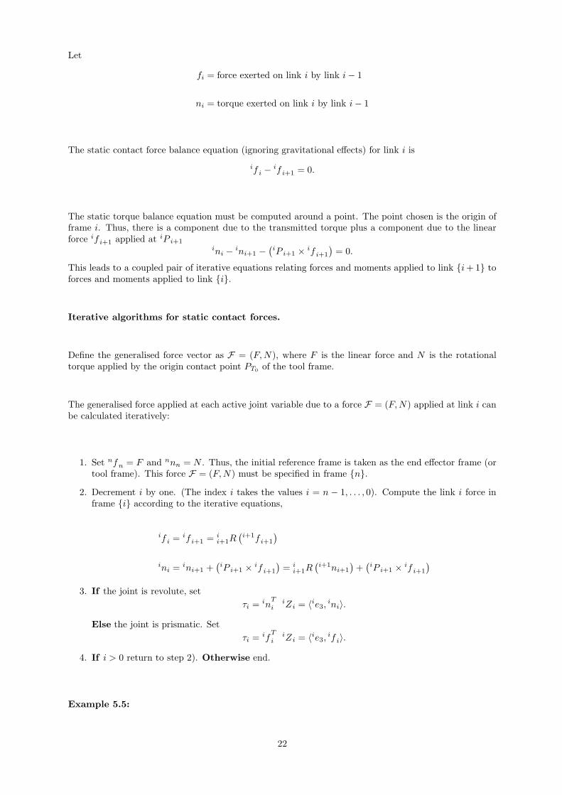
Let

fi = force exerted on link i by link i− 1

ni = torque exerted on link i by link i− 1

The static contact force balance equation (ignoring gravitational effects) for link i is

if i −if i+1 = 0.

The static torque balance equation must be computed around a point. The point chosen is the origin offrame i. Thus, there is a component due to the transmitted torque plus a component due to the linearforce if i+1 applied at iP i+1

ini −ini+1 −

(

iP i+1 ×if i+1

)

= 0.

This leads to a coupled pair of iterative equations relating forces and moments applied to link i+ 1 toforces and moments applied to link i.

Iterative algorithms for static contact forces.

Define the generalised force vector as F = (F,N), where F is the linear force and N is the rotationaltorque applied by the origin contact point PT0

of the tool frame.

The generalised force applied at each active joint variable due to a force F = (F,N) applied at link i canbe calculated iteratively:

1. Set nfn = F and nnn = N . Thus, the initial reference frame is taken as the end effector frame (ortool frame). This force F = (F,N) must be specified in frame n.

2. Decrement i by one. (The index i takes the values i = n − 1, . . . , 0). Compute the link i force inframe i according to the iterative equations,

if i = if i+1 = ii+1R

(

i+1f i+1

)

ini = ini+1 +(

iP i+1 ×if i+1

)

= ii+1R

(

i+1ni+1

)

+(

iP i+1 ×if i+1

)

3. If the joint is revolute, set

τi = inT

iiZi = 〈ie3,

ini〉.

Else the joint is prismatic. Set

τi = ifT

iiZi = 〈ie3,

if i〉.

4. If i > 0 return to step 2). Otherwise end.

Example 5.5:

22

The Force Jacobian

The force Jacobian of a manipulator is defined to be the algebraic mapping between generalised jointforces (torques or linear forces for revolute or prismatic joint respectively) and the Euclidean forcesapplied at the end effector of the robot.

Let F = (F,N) be the linear force (F ) and rotational torque N applied by the origin contact point PT0of

the tool frame. Let τ = (τ1, . . . , τn) denote the generalised forces at each active joint variable (q1, . . . , qn).

τ = JF

Of course F must be expressed with respect to a frame of reference and J must be expressed in the sameframe of reference.

1. The force Jacobian can be computed via an iterative method similar to that used to compute thevelocity Jacobian.

2. The velocity Jacobian of manipulator is also closely linked to the force Jacobian (we explore thisfurther below).

The static force Jacobian concerns only the components of force and torque due to contact of the manip-

ulator with the external world. Gravitational effects are ignored in the following discussion and must bepre-computed and compensated for in any control algorithm based on these ideas.

Principal of virtual work and duality of force and velocity.

The principal of virtual work ensures that the ‘infinitesimal’ work done by the end effector in the toolframe is equal to the total ‘infinitesimal’ work done by the sum of all the active joint variables.

The principal of virtual work yields

〈F , δX〉 = 〈τ, δq〉

where δX denotes an infinitesimal change in the Euclidean position of the end effector of the manipulatorand δq denotes an infinitesimal change in the active joint variables.

Dividing through by δt and limiting one has

δX

δt= nVn,

δq

δt= q

Thus, the work balance equation from above may be written

0FT 0Vn = τT q

23

where both the force exerted by the end effector and its Euclidean velocity must be expressed in the sameframe of reference. The base frame of reference, 0, is chosen for the convenience of the subsequentderivation.

Note: The joint coordinates have only the one representation as a vector of variables. No frame ofreference need be specified.

Velocity Jacobian and the force Jacobian.

Within the workspace of the robot manipulator one has

0Vn = J(q)q

from the definition of the velocity Jacobian.

Substituting into the work balance equation one has

0FTJ(q)q = τT q

and since this is true for all q thenJT (q)0F = τ

Thus, the force Jacobianτ = JF

is given by J = JT (q)τ = JT (q)F .

This is an algebraic expression of the principal of duality of forces and velocities.

Note: The entire discussion undertaken above concerns only contact forces. Forces due to conservativegravitational effects can be explicitly incorporated into the iterative expression or modelled as a changein potential energy in the work balance equation.

Instantaneous transformation of velocities between frames of reference

We have been dealing with the Cartesian velocity V of a rigid body, and we noted it is specified in someparticular frame.

If we are interested in expressing V in some other frame, we need a 6x6 transformation to achieve thismapping.

Consider a rigid-body with two different body-fixed frames A and B attached. The velocity of frameB relative to frame A is zero since the two frames are physically attached to the same rigid body.

24

The velocity of each frame of reference relative to a base frame 0 may be non-zero. Let

XvY = X(

0V)

Y, XωY = X

(

0ω)

Y

for X,Y equal to either A or B

Recalling the velocity propagation equations from earlier one has

(

BvBBωB

)

=

(

BAR −BAR

AP∧

Borg

0 BAR

) (

AvAAωA

)

where recall that AP∧

Borg will be a skew symmetric matrix - the matrix operator corresponding to thecross product.

One writesBVB = B

AT vAVA

Clearly BAT v is a function of BAT hence this result is only valid if there is no relative motion between

frames A and B.

Alternatively, this result can be viewed as the instantaneous velocity transformation BAT v between two

frames of reference if there is relative motion between them (ie. it is valid for a particular BAT .

Transformation of static forces between frames of reference

Using the principal of virtual work once more one has

〈AF ,AVA〉 = 〈BF ,BVB〉

since we assume that the two frames A and B are rigidly fixed together.

Thus, using the instantaneous velocity transformation BAT v, one obtains

AFTAVA = BF

TBVB = BFTBAT v

AVA

25

It follows that

(

AFAANA

)

=

(

BAR −BAR

AP∧

B0

0 BAR

)T (

BFBBNB

)

=

BAR

T0

−(

AP∧

B0

)TBAR

T BAR

T

(

BFBBNB

)

=

(

ABR 0

AP∧

B0

ABR

ABR

) (

BFBBNB

)

= ABT f

BFB

where ABT f is the force-moment transformation.

Summary

Initially looked at velocity kinematics of general rigid bodies with the purpose of applying the tools inthis area to robotic manipulators eg. the 3 components of the velocity of a point in a moving frame.

Looked at deriving the velocity of the end effector of a robotic manipulator as a function of joint rates.Presented an iterative algorithm to do this velocity calculation - starting at the base and moving up tothe end effector

Introduced the velocity Jacobian as the “mapping” between the Cartesian end effector velocity and jointvelocities. Presented an algorithm to derive a velocity Jacobian.

Introduced the idea of a “static” force-torque analysis of a manipulator - in order to determine jointtorques to be applied by the motors. Introduced an algorithm for determining the force/torques on eachlink - starting at the end effector and finishing at the base

Introduced the force Jacobian and investigated its relationship with the velocity Jacobian.

26