Vehicle technologies and bus ﬂeet replacement Author Proof ...

UNCORRECTEDPROOF

1 ORIGINAL PAPER

2 Vehicle technologies and bus fleet replacement

3 optimization: problem properties and sensitivity

4 analysis utilizing real-world data

5 Wei Feng • Miguel Figliozzi

67 � Springer-Verlag Berlin Heidelberg 2014

8 Abstract This research presents a bus fleet replacement optimization model to

9 analyze vehicle replacement decisions when there are competing technologies. The

10 focus of the paper is on sensitivity analysis. Model properties that are useful for

11 sensitive analysis are derived and applied utilizing real-world data from King

12 County (Seattle) transit agency. Two distinct technologies, diesel hybrid and con-

13 ventional diesel vehicles, are studied. Key variables affecting optimal bus type and

14 replacement age are analyzed. Breakeven values and elasticity values are estimated.

15 Results indicate that a government purchase cost subsidy has the highest impact on

16 optimal replacement periods and total net cost. Maintenance costs affect the optimal

17 replacement age but are unlikely to change the optimal vehicle type. Greenhouse

18 gas emissions costs are not significant and affect neither bus type nor replacement

19 age.

20

21 Keywords Bus fleet replacement � Optimization model � Model properties �22 Diesel � Hybrid diesel � Subsidy � Cost elasticity � Breakeven values

23 JEL Classification R41

24

A1 This is a revised and upgraded version of the paper presented at the 12th Conference on Advanced

A2 Systems for Public Transport, Santiago, Chile, July, 2012.

A3 W. Feng � M. Figliozzi (&)

A4 Department of Civil and Environmental Engineering, Portland State University,

A5 P.O. Box 751, Portland, OR 97201, USA

A6 e-mail: [email protected]

A7 W. Feng

A8 e-mail: [email protected]

123Journal : Small-ext 12469 Dispatch : 28-3-2014 Pages : 21

Article No. : 86 * LE * TYPESET

MS Code : PUTR-D-12-00053 R CP R DISK

Public Transp

DOI 10.1007/s12469-014-0086-z

Au

tho

r P

ro

of

UNCORRECTEDPROOF

25 1 Introduction

26 Transit agencies typically own hundreds or thousands of buses; large transit

27 agencies may have multiple fleets of buses with different types of buses serving

28 different routes. For example, King County Metro Transit (KCMT) (Seattle, WA)

29 operates about 1,300 vehicles with multiple bus drivetrain technologies (electric

30 trolley buses, conventional diesel buses, hybrid diesel buses, etc.), sizes and

31 capacities (60 ft. articulate, 30 or 40 ft. standard) and brands/models (New Flyer,

32 Gillig, etc). Fleet capital, operational and maintenance costs are a significant

33 expense for transit agencies. Due to budget and fiscal constraints, it is ever more

34 imperative for transit agencies to manage their fleets in an optimal way without

35 reducing service quality.

36 To minimize fleets total costs over a given time horizon fleet managers have to

37 consider two important tradeoffs. First, as buses age, per-mile operating and

38 maintenance (O and M) costs tend to increase; replacing old vehicles with new ones

39 reduces O and M costs but significantly increases capital costs. Therefore, there is

40 an optimal replacement age (lifecycle) that minimizes the total net cost over a

41 planning time horizon. Second, costs associated to vehicle purchases and per-mile

42 operating, maintenance and fuel costs vary across bus types (conventional diesel,

43 hybrid, electric trolley, etc.), bus designs, and operating environments (congested or

44 not congested routes, hilly or flat routes).

45 In practice, many transit agencies replace their vehicles based on swift yet

46 suboptimal polices derived from rules of thumb, for example every 12 or 20 years

47 or when annual maintenance costs increase above a given threshold. It is possible to

48 formulate and easily solve an integer problem to find the optimal bus type for a

49 specific and constant demand, financial and operating environment. In the case of

50 KCMT, analysts were not interested just in an optimal solution but in obtaining a

51 better understanding of the key variables and factors affecting the relative

52 competitiveness of diesel and hybrid vehicles.

53 The contributions of this study are to develop and use a fleet replacement

54 model in a way that is suitable for decision makers and sensitivity analysis.

55 More specifically, the contributions of this research are to: (1) present an

56 optimization model to minimize fleet costs that are relevant to decision makers;

57 (2) study properties of the optimization model that can facilitate the sensitivity

58 analysis; (3) apply the model and properties to real-world KCMT data for

59 60- ft. diesel bus and hybrid diesel bus fleets; and (4) study the impacts of

60 government purchase cost subsidy and other input variables on the optimal

61 replacement decisions.

62 The reminder of this paper is organized as follows: Sect. 2 briefly reviews

63 bus fleet replacement practices and replacement optimization models. Section 3

64 presents the model formulation. In Sect. 4 model properties are explored.

65 Section 5 describes KCMT bus fleet data. Section 6 shows baseline scenario

66 results. Section 7 presents sensitivity analysis results. Finally, Sect. 8 wraps up

67 with conclusions.

W. Feng, M. Figliozzi




Au

tho

r P

ro

of

UNCORRECTEDPROOF

68 2 Literature review

69 Previous studies in the public transport field have shown how fuel efficiency and

70 operating and maintenance costs change when vehicles age; significant differences

71 have been found across bus models, transit agencies and service environments

72 (Lammert 2008; Chandler and Walkowicz 2006; Schiavone 1997). Bus life cycle

73 costs have been previously compared across bus engine types and design models

74 (Clark et al. 2007; Laver et al. 2007; Clark et al. 2009; Kim et al. 2009). The papers

75 referenced in this paragraph focus on vehicle characteristics and lifecycle costs

76 assuming a constant replacement age. Optimal replacement schedules and bus type

77 choice that minimize bus fleet total net cost have not been studied in the previously

78 stated references.

79 There is a large body of literature dealing with vehicle replacement optimization

80 models in the operations research field. These models can be broken into two

81 categories depending on whether buses in a fleet are homogeneous or heteroge-

82 neous. In homogeneous models, the objective is to find the best bus replacement age

83 for a set of identical vehicles, in other words, buses with the same type and age have

84 to be replaced together (also known as the ‘‘no cluster splitting rule’’). These models

85 are usually solved using a dynamic programming (DP) approach (Bellman 1955;

86 Oakford et al. 1984; Bean et al. 1984; Bean et al. 1994; Hartman 2001; Hartman and

87 Murphy 2006). Dynamic programming has the advantage of allowing the

88 consideration of probabilistic distributions for some state variables such as

89 utilization or operational costs.

90 Heterogeneous models are more appropriate when multiple bus fleets have to be

91 optimized simultaneously or when budget constraints are needed. For example, the

92 ‘‘no cluster splitting rule’’ cannot be applied when vehicles of the same type and age

93 may be replaced in different years due to budget limitations. These models are able

94 to solve more practical problems but input variables are usually deterministic.

95 Stochastic heterogeneous models are difficult to solve. Most heterogeneous models

96 employ integer programming (IP) formulations (Simms et al. 1984; Karabakal et al.

97 1994; Hartman 1999, 2000, 2004). With additional assumptions a DP approach can

98 be applied to heterogeneous problems (Jones et al. 1991). None of these theoretical

99 models mentioned in this paragraph deals real world fleet data.

100 Fan et al. (2012) developed a fleet optimization framework using a DP approach;

101 however the simultaneous optimization of heterogeneous vehicles and sensitivity

102 analysis of input variables were not addressed. Figliozzi et al. (2011), Feng and

103 Figliozzi (2013) adopted IP models to study a fleet of heterogeneous passenger cars

104 and delivery trucks with real world operational data. Impacts of policy, market,

105 utilization, emissions, and technological factors were analyzed using scenario

106 analysis and elasticity analysis. Boudart and Figliozzi (2012) studied how economic

107 and technological factors affect a single bus optimal replacement age.

108 Summarizing, several papers have described the use of optimization models to

109 solve real world problems. Keles and Hartman (2004) adopted an IP model in a

110 transit fleet replacement problem with multiple types of buses. The optimization

111 model used in this paper is deterministic and it is derived from the models

112 developed by Hartman (2000); Keles and Hartman (2004). However, unlike these

Vehicle technologies and bus fleet replacement optimization




Au

tho

r P

ro

of

UNCORRECTEDPROOF

113 two references, the objective function incorporates emissions costs and all the

114 model parameters used in the paper are based on real-world data; in addition, this

115 paper derives breakeven analysis properties and presents a thorough sensitivity

116 analysis based on key vehicle characteristics, costs and utilization levels. The

117 contribution of this paper is a first step that facilitates a better understanding of the

118 key parameters of the problem. A more complete analysis should include stochastic

119 models but this type of models is beyond the scope of this research.

120 3 Methodology

121 In the optimization model, five major cost components are considered: capital

122 (purchase) costs, salvage revenue (represented as a negative cost), energy (fuel)

123 costs, maintenance costs, and emissions costs. The objective function of this model

124 is to minimize the discounted sum of all five costs for all buses over a planning time

125 horizon. The decision variables are when and which buses should be replaced with

126 what type of new buses. Once the optimal solution is found, costs breakdowns and

127 bus utilization statistics can be easily calculated. The optimization approach is

128 depicted in Fig. 1.

Fig. 1 Bus fleet replacement optimization framework





Au

tho

r P

ro

of

UNCORRECTEDPROOF

129 The optimization model requires three categories of inputs: economic factors,

130 vehicle characteristics, and initial fleet configuration. Economic factors include

131 planning time horizon, annual number of vehicles (demand) or annual miles that

132 must be traveled, discount rate, and forecasted fuel costs. Vehicle factors include

133 types of buses and for each bus type, its maximum physical life, purchase cost and

134 salvage value as a function of age, fuel economy as a function of age, annual

135 utilization (miles traveled) as a function of age, and per-mile maintenance cost as a

136 function of age and annual utilization. Initial fleet configuration includes the type,

137 age, and number of existing buses. Once the inputs are specified, the model can

138 provide optimal replacement policies.

139 The optimization model is formulated as a deterministic heterogeneous fleet

140 replacement model, which means all input variables are known with certainty.

141 3.1 Indices

142 Type of bus: k 2 K ¼ 1; 2; . . .;Kf g:143 Age of a bus type k in years: i 2 Ak ¼ 0; 1; 2; . . .;Akf g,144 Time periods: j 2 T ¼ f0; 1; 2; . . .; Tg; and

145 3.2 Decision variables

146

148 Xijk ¼149 The number of i-year old, k-type buses used in year j,

150 Yijk ¼151 The number of i-year old, k-type buses salvaged at the end of year j, and

152 Pjk ¼153 The number of k-type buses purchased at the beginning of year j:154

155 3.3 Parameters

156 3.3.1 (a) Constraints

157

159 Ak ¼160 Maximum age of bus type k (it must be salvaged when a bus reaches this

161 age),

162 uik ¼163 Utilization (annual miles traveled by an i-year old, k-type bus),

164 dj ¼165 Demand (miles traveled by all buses) in year j;

166 bj ¼167 Budget (available for purchasing new buses) constraint in year j;168

169 3.3.2 (b) Cost or revenue

170

172 vk ¼173 Purchase cost of a k-type bus,

174 fik ¼175 Fuel economy (mpg) for an i-year old, k-type bus,

176 fcj ¼177 Fuel price($/gallon) in year j,

178 mik ¼179 Per-mile maintenance cost for an i-year old, k-type bus,

180 sik ¼181 Salvage revenue (negative cost) from selling an i-old, k-type bus,





Au

tho

r P

ro

of

UNCORRECTEDPROOF

182 ec ¼ Emissions cost per ton of GHG,

183 d ¼ Discount rate.

184

185 3.3.3 (c) Emissions

186

187 eik ¼ Utilization emissions in GHG equivalent tons per mile for an i-year old, k-

type bus, and

188

189 3.3.4 (d) Initial conditions

190

191 hik = The number of i-year old, k-type buses available at the beginning.

192

193 3.4 Objective function

194

min Z ¼XT�1

j¼0

XK

k¼1vk �Pjk þ

XAk�1

i¼0

fcj

fikþmik þ ec � eik

� �

uik �Xijk

� �

� 1þ dð Þ�j

þXT

j¼0

XK

k¼1

XAk

i¼1sikYijk 1þ dð Þ�j

ð1Þ

196196197 3.5 Constraints

198

XK

k¼1vjk � Pjk � bj; 8j 2 0; 1; 2; . . .; T � 1f g ð2Þ

200200XAk�1

i¼0

XK

k¼1Xijk � uik � dj; 8j 2 0; 1; 2; . . .; T � 1f g ð3Þ

202202 Pjk ¼ X0jk; 8j 2 1; 2; . . .; T � 1f g; 8k 2 K ð4Þ

204204 P0k þ h0k ¼ X00k; 8k 2 K ð5Þ

206206 Xi0k þ Yi0k ¼ hik8i 2 1; 2; . . .;Akf g; 8k 2 K ð6Þ

208208 X i�1ð Þðj�1Þk ¼ Xijk þ Yijk; 8i 2 1; 2; . . .;Akf g; 8j 2 1; 2; . . .; Tf g; 8k 2 K ð7Þ

210210 XiTk ¼ 0; 8i 2 0; 1; 2; . . .;Ak � 1f g; 8k 2 K ð8Þ

212212 XAk jk ¼ 0; 8j 2 0; 1; 2; . . .; Tf g; 8k 2 K ð9Þ

214214 Y0jk ¼ 0; 8j 2 0; 1; 2; . . .; Tf g; 8k 2 K ð10Þ

216216 Pjk;Xijk; Yijk 2 I ¼ 0; 1; 2; . . .f g ð11Þ

217218 The objective function, expression (1), minimizes the sum of purchasing, energy

219 (fuel), maintenance, salvage, and emissions costs over the period of analysis, i.e.





Au

tho

r P

ro

of

UNCORRECTEDPROOF

220 from time zero (present) to the end of year T; there is no fixed purchase costs

221 associated to the purchase of vehicles. Purchase costs cannot exceed the annual

222 budget, expression (2). The number of vehicles in the fleet at any time must equal or

223 exceed the minimum needed to cover the demand in terms of annual number of

224 buses or annual miles traveled, expression (3). The number of vehicles purchased

225 must equal the number of new vehicles for each vehicle type and year, except for

226 year zero, expression (4). The number of new vehicles utilized during year zero

227 must equal the sum of existing new vehicles plus purchased vehicles, expression (5).

228 Similarly, expression (6) ensures the conservation of vehicles (i.e. the initial

229 vehicles—not 0-age ones—must be either used or sold). The age of any vehicle in

230 use will increase by 1 year; after each time period vehicles are either used or sold

231 (7). At the end of the last time period, all vehicles will be sold at the corresponding

232 salvage value (8). When a vehicle reaches its maximum age, the vehicle must be

233 sold (9). A newly purchased vehicle should not be sold before being used at least

234 1 year (10). Finally, the decision variables associated with purchasing, utilization,

235 and salvaging decisions must be integer non-negative numbers, expression (11).

236 4 Model sensitivity analysis properties: breakeven points

237 The model described in the previous section can provide the optimal vehicle

238 replacement schedule given a set of deterministic input parameters. However,

239 decision makers usually want to know not only the optimal solution but also the

240 sensitive of the optimal solution. For example, decision makers can be interested in

241 understanding the breakeven values that delimit the competitiveness of each vehicle

242 type (diesel vs. hybrids). In particular, USA transit agency managers are interested

243 in FTA subsidy levels and how they impact the optimal vehicle type. In this case, a

244 purchase cost subsidy breakeven value indicates when the optimal vehicle type

245 changes as function of the subsidy level when holding all other input parameters

246 constant (ceteris paribus). In this section, as in the model presented in Sect. 3, we

247 assume that there are no budget constraints.

248 We define that there is a breakeven value for a parameter (e.g. government

249 subsidy) for vehicle types k and k’ when the value of the objective function (1) is the

250 same when: (a) P0k ¼ n, P0k0 ¼ 0 and (b) P0k ¼ 0, P0k0 ¼ n where n is an integer

251 number. The definition of the breakeven value indicates that the objective function

252 value is the same when only one type of the vehicle (either k or k’ but not both) is

253 purchased in year zero. The definition does not guarantee that (1) there exists at least

254 one breakeven value, (2) that this value is unique, and that (3) there is an efficient

255 procedure to obtain breakeven values. This section defines under what conditions

256 and assumptions it is possible to find unique breakeven values.

257 For any given feasible replacement policy p given by the sets of decision

258 variables (Pjk;Xijk;Yijk), let the subsidy level be denoted by s, with 0� s� 1, and

259 the total replacement policy costs for policy p and subsidy s be denoted by fðp; sÞ.

260 Property 1 The total net cost fðp; sÞ as a function of the subsidy level s for a given261 replacement policy p is a linear decreasing function in the interval 0� s� 1.





Au

tho

r P

ro

of

UNCORRECTEDPROOF

262 Proof It is possible to write fðp; sÞ as:

f p; sð Þ ¼X

T�1

j¼0

X

K

k¼1

vkð1� sÞ � Pjk þX

Ak�1

i¼0

fcj

fikþ mik þ ec � eik

� �

uik � Xijk

" #

� 1þ dð Þ�jþX

T

j¼0

X

K

k¼1

X

Ak

i¼1

sikYijk 1þ dð Þ�j

264264 Then, if p = (Pjk;Xijk;Yijk) is a replacement policity, then its cost for a certain

265 level of subsidy, f p; sð Þ; can be rewritten as the sum of a constant term and a liner

266 decreasing function in the interval 0� s� 1.

f p; sð Þ ¼ g pð Þ � sX

T�1

j¼0

X

K

k¼1

ðvk � PjkÞ � 1þ dð Þ�j

267

268 where g pð Þ is a constant term that does not depend on the value of s.

269

g pð Þ ¼XT�1

j¼0

XK

k¼1vk � Pjk þ

XAk�1

i¼0

fcj

fikþ mik þ ec � eik

� �

uik � Xijk

� �

� 1þ dð Þ�j

þXT

j¼0

XK

k¼1

XAk

i¼1sikYijk 1þ dð Þ�j

271271 In this property it is also assumed that purchase prices are positive.

272 Property 2 For a given vehicle type k, the minimum of the total net cost fk p; sð Þ as273 a function of the subsidy level s is a decreasing concave function in the interval

274 0� s� 1.

275 Proof Let Pk be the set of all feasible replacement policies (Pjk;Xijk;Yijk) for a

276 given vehicle type k. Then, let’s denote Zk sð Þ as the minimum total net cost function

277 for vehicle type k for a given subsidy level s; 0� s� 1:

Zk sð Þ ¼¼ minf p; sð Þ for 8p 2 Pk

278

279 The function Zk sð Þ is a concave and decreasing function in the interval 0� s� 1

280 because the minimum of a set of linear functions is a concave function and also

281 because each one of the fk p; sð Þ functions is a decreasing function in the interval

282 0� s� 1.283

284

285 Property 3 Given two different vehicle types k and k’ and functions Zk sð Þ and

286 Zk0 sð Þ such that Zk s ¼ 0ð Þ\Zk0 s ¼ 0ð Þ and Zk s ¼ 1ð Þ[ Zk0 s ¼ 1ð Þ then the

287 functions cross at least at one point.

288 Proof Zk sð Þ and Zk0 sð Þ are continuous concave decreasing functions since they are

289 obtained as the minimum of a set of continuous decreasing linear functions. Then,

290 applying the Bernard Bolzano theorem (also known as the intermediate value

291 theorem), there is a point in the interval 0� s� 1. Because the functions are

292 continuous and decreasing, the crossing value will be found in the interval





Au

tho

r P

ro

of

UNCORRECTEDPROOF

293 (Zk s ¼ 1ð Þ; Zk s ¼ 0ð ÞÞ.294 Because the functions and concave, continuous and decreasing in the interval

295 0; 1½ �, the breakeven value is unique.

296 Lemma 1 Given two different vehicle types k and k’ and functions Zk sð Þ and

297 Zk0 sð Þ such that Zk s ¼ 0ð Þ\Zk0 s ¼ 0ð Þ and Zk s ¼ 1ð Þ[ Zk0 s ¼ 1ð Þ then it is

298 possible to apply a bisection method search procedure and obtain a crossing point.

299 Proof The bisection method converges to a root of a function h(x) if the function is

300 continuous in a given interval [a,b] and h(a) and h(b) have opposite signs. By

301 defining h sð Þ ¼ Zk sð Þ � Zk0 sð Þ the result is a continuous function where h 0ð Þ and

302 h 1ð Þ have opposite signs.

303 The importance of the Lemma 1 is that usually when comparing two rival

304 technologies, e.g. hybrid diesel and conventional diesel, costs are such that

305 Zk s ¼ 0ð Þ\Zk0 s ¼ 0ð Þ and Zk s ¼ 1ð Þ[ Zk0 s ¼ 1ð Þ; where type k is the ‘‘cheap’’

306 technology with lower capital costs but higher operating costs and k’ is the

307 ‘‘expensive’’ but more efficient technology with higher initial capital costs but lower

308 operations/maintenance costs. If Zk s ¼ 0ð Þ\Zk0 s ¼ 0ð Þ and Zk s ¼ 1ð Þ\Zk0 s ¼ 1ð Þ309 then the choice is trivial since technology k dominates technology k’.

310 It is possible to implement the IP model formulated in the previous section within

311 a bisection algorithm; given Lemma 1 the algorithm will converge and find a

312 breakeven point. The existence of breakeven points and the certain convergence can

313 be also extended to other parameters such as fuel/energy costs that will generate

314 linear or concave cost functions that are increasing functions in an interval. The

315 properties studied in this section are applied in the sensitivity analysis section.

316 5 Basic scenarios

317 There are three types of parameters or inputs: vehicle, economic, and initial fleet

318 configuration parameters. This section describes the parameters, based on real-

319 world KCMT data, used in this research.

320 5.1 Vehicle parameters

321 The two vehicle technologies (types) are hybrid diesel and conventional diesel. The

322 vehicles compared are both New Flyers (http://www.newflyer.com/), the New Flyer

323 60 ft. hybrid diesel bus (k ¼ 1) and the New Flyer 60 ft. conventional diesel bus

324 (k ¼ 2).

325 A1 ¼ A2 ¼ 20. The maximum ages are assumed to be 20 years for both buses;

326 most transit agencies in the US replace buses in a 12–16-year cycle (Laver et al.

327 2007).

328 v1 ¼ $958,000, v2 ¼ $737,000. The purchase costs for the two buses are

329 $958,000 for hybrid bus and $737,000 for diesel bus, including ordering costs and

330 communication/data collection equipment. Also, transit agencies can receive

331 purchase cost subsidies from the US Federal Transit Administration (FTA).

332 However FTA adds additional age replacement constrains; for example, if an 80 %





Au

tho

r P

ro

of

http://www.newflyer.com/

UNCORRECTEDPROOF

333 purchase cost subsidy is received the bus must be kept for a minimum of 12 years.

334 This can be added to the model as a new constraint shown in equation.

335 sik ¼ �$1; 000; 8k 2 K; i 2 Ak. The salvage values for the two buses are

336 assumed to be $1,000 regardless of bus type or bus age according to KCMT request.

337 fi1 ¼ 3:65mpg, fi2 ¼ 2:50mpg, 8i 2 Ak. The KCMT data indicate that the hybrid

338 bus fuel economy is 3.65 mpg and the diesel bus is 2.50 mpg on average if they

339 were operated in the same existing routes; fuel economy does not significantly vary

340 with age.

341 uik ¼ 33; 045miles=year; 8k 2 K; i 2 Ak. Because the two competing buses will

342 serve the same bus route, their annual utilizations will be similar. Statistical data

343 shows that the average annual miles traveled per bus is 33,045 miles.

344 ei1 ¼ 2:504 kg=mi; ei2 ¼ 3:407 kg=mi; 8i 2 Ak. Only the tailpipe CO2 emissions

345 are considered in the model and the generation rates are 2.504 kg/mile for hybrid

346 buses and 3.407 kg/mile for diesel buses regardless of age but a function of fuel

347 economy, see also Clark et al. (2007).

348 To estimate per-mile maintenance cost as a function of age and utilization a

349 regression model was estimated utilizing three independent variables: vehicle

350 utilization, age, and vehicle type. The general administrative and operating costs

351 (overhead) are constant and independent of the chosen vehicle technology and

352 therefore excluded from the per-mile maintenance costs. In general, bus per-mile

353 maintenance cost increases with both age and cumulative utilization. Though, these

354 two variables are highly correlated in practice; hence, the per-mile maintenance cost

355 is expressed solely as a function of age. In the model age is associated to the

356 additional uk miles traveled by a bus per year.

357 According to the baseline annual utilization uik ¼ $ 33; 045miles=year;358 8k 2 K; i 2 Ak, for this utilization, the estimated per-mile maintenance cost

359 functions for hybrid and diesel buses are:

mi1 ¼ 0:530þ 0:0867� i;mi2 ¼ 0:372þ 0:0673� i; 8i 2 0; 1; . . .;Ak � 1f g; 8k2 K

361361362 5.2 Economic parameters

363 T ¼ 100. A long planning time horizon of 100 years was used to abate the effect of

364 the last incomplete vehicle life cycle on the first optimal bus type choice. Because

365 the maximum age is 20 year, there are at least five replacements which ensure that

366 the impact of the planning horizon length is negligible. Furthermore, due to the

367 compound interest and given realistic discount rates of 4 % or higher the discounted

368 annual costs quickly decrease after year ten.

369 d ¼ 9:55%. A 7.0 % annual discount rate (APR) for capital investments and

370 2.55 % consumer price index (CPI) are assumed throughout the planning time

371 horizon following KCMT policies; these assumptions yield a 9.55 % nominal

372 annual discount rate.

373 fcj ¼ fc0 � ð1þ 2:6%Þ j; 8j 2 T. Three fuel price (fc0=$2.64/gal, $3.48/gal and

374 $4.46/gal) forecast functions are utilized following a recent report (Parametrix and





Au

tho

r P

ro

of

UNCORRECTEDPROOF

375 LTK Engineering Servies 2011) and forecasts based on long-term oil-price

376 projections from US Energy Information Administration (2011).

377 ec ¼ $30/ton. CO2 emissions penalty costs (suggested by KCMT) are used to

378 account for the impact of emissions costs on optimal replacement decision.

379 bj ¼ þ1; 8j 2 T. Transit agencies like KCMT usually purchase a group of buses

380 in certain years instead of purchasing only a few buses annually; in addition there is

381 a limit on the total number of bus types. Having one bus type simplifies maintenance

382 and fleet management (for example, less spare parts are specialized mechanics are

383 needed among other benefits). In this case, budget constraints are not considered,

384 typically federal subsidies are received or a bond pays for the new vehicles.

385 dj ¼ uik; 8j 2 T; k 2 K; i 2 Ak. Because there are no budget constraints, for

386 convenience and to facilitate the analysis of bus type tradeoffs replacement results

387 are presented on a per bus basis.

388 5.3 Initial fleet parameters

389 KCMT was interested in analyzing what type of bus will be the best choice for its

390 fleet 60-foot buses that must be replaced by the end of 2013. To simplify spare part

391 inventories and maintenance operations, by limiting the number of bus types/

392 models/brands, all the old buses are replaced by new ones. The question is: what

393 type of new bus, diesel or hybrid? Therefore, for the scenario analysis and

394 sensitivity report we can then assume that all existing vehicles are sold at the end of

395 2013 and new ones will be purchased at the beginning of the following year

396 (hik ¼ 0; 8k 2 K; i 2 Ak). The reader is reminded that there is no fixed cost charge

397 per purchase and that all the buses purchased at year zero will be replaced at the

398 same time.

399 6 Baseline scenario results

400 Given the data presented in the previous section, the problem thus becomes, which

401 new bus type should KCMT buy in 2014 to minimize future fleet total net costs, the

402 New Flyer 60 ft. hybrid bus or the New Flyer 60 ft. diesel bus? What will be the

403 optimal replacement cycle?

404 The optimization model was implemented using a Python interface; Cplex 12.4

405 was used to solve the integer programming model. Results for two baseline

406 scenarios (no subsidy and 80 % subsidy) are shown in Figs. 2, 3.

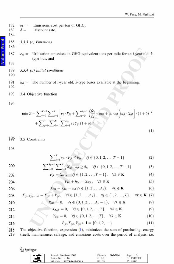
407 The net present value (NPV) of the five cost components and their sum (total net

408 cost) are shown for both scenarios. Figure 2 presents the no subsidy scenario where

409 the optimal solution is to choose diesel bus and replace it every 20 years with a total

410 net cost is $1.546 million; if an alternative replacement is chosen (choose hybrid bus

411 and replace it every 20 years), the total net cost would be $1.688 million. Therefore,

412 the savings per bus is approximately $0.142 million. For a fleet with 300 vehicles,

413 almost $42.6 million can be saved from choosing the optimal replacement solution.

414 In this no subsidy scenario, the purchase cost has the highest percent share (57 %) of





Au

tho

r P

ro

of

UNCORRECTEDPROOF

415 the total net costs. Hence, the optimal solution tends to extend bus life cycle as long

416 as possible (the maximal age of 20 years is bounding in this case).

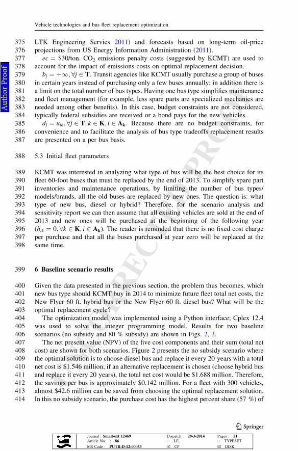
417 Figure 3 shows the results of the maximum subsidy scenario results (80 % in the

418 USA). In this scenario the optimal bus type switched to hybrid bus and the optimal

419 replacement cycle decreased to 14 years. Because the purchase cost has been

420 reduced significantly, the fuel cost difference becomes the dominant factor. The

421 saving is of approximately $34,000 per bus or $10.2 million for a fleet with 300

422 vehicles. Also, because the initial purchase cost is reduced significantly, the optimal

423 replacement cycle has decreased from over 20 to just 14 years. Results indicate that

424 a 80 % government bus purchase subsidy greatly affects total costs and optimal

425 replacement type and age.

-$0.2

$0.0

$0.2

$0.4

$0.6

$0.8

$1.0

$1.2

$1.4

$1.6

$1.8

Total cost Purchase

cost

Fuel cost maintenance

cost

emissions

cost

Salvage

revenue

Millio

ns

No subsidy

Alternative: Hybrid 20 years

Optimal: Diesel 20 years

Fig. 2 Total net cost and cost breakdown for no subsidy scenario

-$0.2

$0.0

$0.2

$0.4

$0.6

$0.8

$1.0

$1.2

$1.4

$1.6

$1.8

Total cost Purchase cost Fuel cost maintenance

cost

emissions

cost

Salvage

revenue

Mil

lio

ns

80% subsidy

Optimal: Hybrid 14 years

Alternative: Diesel 14 years

Fig. 3 Total net cost and cost breakeven for 80 % subsidy scenario





Au

tho

r P

ro

of

UNCORRECTEDPROOF

426 7 Sensitivity analysis

427 The effects of each input variable on the optimal bus type, replacement cycle, and

428 total net cost are evaluated individually by holding all other input variables in the

429 baseline scenarios constant (i.e. ceteris paribus).

430 7.1 Impacts of key input parameters on optimal bus type and lifecycle

431 7.1.1 Fuel price

432 To investigate the impacts of uncertain fuel prices on the optimal replacement plan,

433 a wide range of potential fuel prices (between $2.64/gal and $4.46/gal) are tested

434 with both 0 and 80 % subsidy levels. Results are shown in Table 1.

435 Results indicate that with a 0 % purchase cost subsidy, the optimal solution is

436 always to choose the diesel bus and replace it every 20 years. In other words, when

437 there is no purchase cost subsidy, fuel price has no impact on the optimal

438 replacement solution within realistic values.

439 With an 80 % cost subsidy, if the fuel price is very low (less than $2.78/gal) the

440 optimal solution is to choose diesel bus and replace it every 13 or 12 years. If the

441 fuel price is more than $2.78/gal the optimal solution is to choose a hybrid bus and

442 replace it every 14 years. Optimal solutions are more sensitive to low fuel prices

443 when there is a high purchase cost subsidy.

444 7.2 Fuel economy

445 According to the data provided by KCMT, the 60 ft. New Flyer hybrid bus fuel

446 economy varies slightly between 3.59 mpg and 3.69 mpg and the 60 ft. New Flyer

447 diesel bus fuel economy varies between 2.39 and 2.58 mpg. To investigate the

448 impact of relative fuel economies between diesel and hybrid buses different fuel

449 economies were optimized. Sensitivity results are summarized in Table 2.

450 The number in the table, ‘‘14H’’ for example, indicates that the optimal solution

451 is to choose a hybrid bus and replace it every 14 years. Table 2 shows how optimal

452 replacement solutions change with varying diesel and hybrid bus fuel economies in

453 both 0 and 80 % purchase cost subsidy scenarios. Without a purchase cost subsidy,

454 the optimal solution remains to choose the diesel bus and replace it every 20 years

455 even if: (a) diesel bus fuel economy decreases to 2.2 mpg holding hybrid bus fuel

456 economy constant as 3.65 mpg, or (b) hybrid bus fuel economy increases to

457 3.95 mpg holding diesel bus fuel economy constant as 2.5 mpg. This indicates that

458 diesel buses are significantly better than hybrid buses in the 0 % subsidy scenario

Table 1 Impacts of fuel price on optimal replacement plan

Fuel price

($/gal)

2.64 2.78 2.92 3.06 3.20 3.34 3.48 3.62 3.76 3.90 4.04 4.18 4.32 4.46

0 % subsidy 20D 20D 20D 20D 20D 20D 20D 20D 20D 20D 20D 20D 20D 20D

80 % subsidy 13D 12D 14H 14H 14H 14H 14H 14H 14H 14H 14H 14H 14H 14H





Au

tho

r P

ro

of

UNCORRECTEDPROOF

459 even with high variability in the relative fuel economies between the two bus

460 technologies.

461 In the 80 % subsidy scenario, the best bus type is a function of the relative fuel

462 economies between the two bus types. When the hybrid bus fuel economy is 35 %

463 higher than the diesel bus fuel economy, hybrid buses are preferred; when the

464 difference is less than 35 %, diesel buses are preferred. The reader should recall that

465 the baseline relative fuel economy between hybrid and diesel bus is approximately

466 46 % for average fuel economy values (3.65 vs. 2.50 mpg).

467 7.3 Annual utilization

468 Historical data provided by KCMT indicated that the average annual utilization

469 ranges between 28,379 and 39,679 miles per bus. Therefore, to investigate whether

470 and how annual utilization affects the optimal replacement solutions, different

471 annual utilizations are tested from 28,379 to 39,679 miles/year/bus. Results are

472 summarized in Table 3. Note that per-mile maintenance cost functions were

473 updated to account for varying annual utilization levels.

474 Results show that in the 0 % subsidy scenario the optimal solution is always to

475 choose the diesel bus and replace it every 20 years (not affected by the annual

476 utilization within the examined range). However, in the 80 % subsidy scenario, the

477 optimal solution is always to buy hybrid buses but the optimal replacement cycle

478 decreases from 16 to 12 years as the annual utilization increases (per-mile

479 maintenance cost increases faster with age with higher annual utilization).

Table 2 Impacts of diesel bus fuel economy on optimal replacement plan

Diesel (mpg) hybrid 3.65 mpg 2.2 2.3 2.4 2.5 2.6 2.7 2.8

0 % subsidy 20D 20D 20D 20D 20D 20D 20D

80 % subsidy 14H 14H 14H 14H 14H 13D 14D

Hybrid (mpg) diesel 2.5 mpg 3.35 3.45 3.55 3.65 3.75 3.85 3.95

0 % subsidy 20D 20D 20D 20D 20D 20D 20D

80 % subsidy 13D 14H 14H 14H 14H 14H 14H

Table 3 Impacts of annual utilization on optimal bus choice and lifecycle

Annual

utilization

(miles/

year/bus)

28,379 29,509 30,639 31,769 32,899 34,029 35,159 36,289 37,419 38,549 39,679

0 %

subsidy

20D 20D 20D 20D 20D 20D 20D 20D 20D 20D 20D

80 %

subsidy

16H 15H 15H 14H 14H 13H 13H 12H 12H 12H 12H





Au

tho

r P

ro

of

UNCORRECTEDPROOF

480 7.3.1 Capital purchase cost

481 Capital costs can vary due to market fluctuations, technology improvements, and

482 purchase quantity. It has also been shown in the baseline scenario results that

483 purchase costs may have a significant share of total life cycle costs. Therefore, it is

484 necessary to evaluate the sensitive the optimal replacement plans as a function of

485 varying capital purchase costs. Up to 20 % under and over the current purchase cost

486 for diesel and hybrid buses are tested and results are shown in Table 4.

487 Results from Table 4 indicate that if there is no subsidy, the optimal solution is

488 always to choose diesel buses and replace them every 20 years except when the

489 diesel bus price increases 20 % or more holding hybrid bus price constant.

490 Alternatively, when the hybrid bus price decreases 15 % or more holding diesel bus

491 price constant it is better to choose hybrid buses. The reader is reminded that there is

492 no fixed cost charge per purchase and that all the buses purchased at year zero are

493 replaced at the same time.

494 In the 80 % subsidy scenario, the optimal bus type is always hybrid except for

495 diesel bus price reductions of 20 % or more (holding hybrid bus price constant) or

496 when hybrid bus price increases 15 % or more holding diesel bus price constant.

497 The optimal replacement cycle increases slightly with increasing purchase cost for

498 each optimal bus.

499 7.3.2 Initial age and bus type

500 The baseline scenarios assume that there are no existing buses. However, it is

501 interesting to evaluate scenarios with an existing fleet of buses of different ages.

502 Scenarios with different initial fleet configurations (types and ages) are also tested.

503 The initial fleet configurations is assumed to be one bus, hybrid or diesel bus, with

504 any of the following six ages: 3, 6, 9, 12, 15, and 18. Results for the 24 scenarios are

505 shown in Tables 5, 6.

506 Results indicate that initial age has little impact on replacement age or optimal

507 bus type. In the 80 % subsidy scenario, if the initial bus is a hybrid, the optimal

508 solution will be to keep using the hybrid bus and replace it every 16 years. If the

509 initial bus is diesel, the optimal solution will be to keep using the diesel bus until it

Table 4 Impacts of capital purchase cost on optimal replacement plan

Diesel bus price % change

(hybrid: $958,000)

-20 % -15 % -10 % -5 % 0 % 5 % 10 % 15 % 20 %

0 % subsidy 20D 20D 20D 20D 20D 20D 20D 20D 20H

80 % subsidy 12D 14H 14H 14H 14H 14H 14H 14H 14H

Hybrid bus price % change

(diesel: $737,000)

-20 % -15 % -10 % -5 % 0 % 5 % 10 % 15 % 20 %

0 % subsidy 20H 20H 20D 20D 20D 20D 20D 20D 20D

80 % subsidy 12H 12H 13H 13H 14H 14H 14H 12D 13D





Au

tho

r P

ro

of

UNCORRECTEDPROOF

510 reaches age 12 (or age 15 or 18 if the initial diesel bus age is already 15 or 18), and

511 then replace it with a hybrid bus every 16 years in all future years in the time

512 horizon. In the 80 % subsidy case, the optimal bus is the hybrid, even if the initial

513 bus if a diesel there is always a reversion towards the optimal policy. In the 0 %

514 subsidy scenario the opposite takes place.

515 7.3.3 Subsidy level

516 Results indicate that the 0 and 80 % subsidy levels lead to different optimal bus type

517 choices and replacement cycle. It is interesting to investigate how the optimal

518 replacement plan changes with subsidy level. Ten subsidy levels (from 0 to 90 %

519 with 10 % interval) were tested and the results are shown in Table 7.

520 Results indicate that with less than 50 % purchase subsidy, the optimal solution

521 is always to purchase diesel bus and replace it every 20 years; with 60 % purchase

522 subsidy, the optimal solution is still diesel bus but the optimal replacement cycle

523 decreases to 19 years. When purchase subsidy increased to 70 %, the optimal bus

524 type switched to hybrid bus because the additional capital cost of purchasing a

525 hybrid bus is smaller than the benefit (higher fuel efficiency and less fuel cost) of

526 utilizing a hybrid bus, the replacement cycle also decreased to 18 years. And as the

527 purchase subsidy level reaches to high level, the optimal replacement cycle

528 decreased rapidly.

Table 5 Impacts of initial fleet configuration on optimal replacement plan (80 % subsidy)

Diesel FE (mpg) 2.50 mpg 3.32 mpg

Initial bus age (hybrid) 3 6 9 12 15 18 3 6 9 12 15 18

Hybrid replacement age 16 16 16 16 16 18 16 16 16 16 16 18

Diesel replacement age – – – – – – – – – – – –

Initial bus age (diesel) 3 6 9 12 15 18 3 6 9 12 15 18


Diesel replacement age 12 12 12 12 15 18 15 15 15 15 15 18

In italics a one-time replacement

Table 6 Impacts of initial fleet configuration on optimal replacement plan (0 % subsidy)

Diesel FE (mpg) 2.50 mpg 3.32 mpg

Initial bus age (hybrid) 3 6 9 12 15 18 3 6 9 12 15 18



Initial bus age (diesel) 3 6 9 12 15 18 3 6 9 12 15 18

Hybrid replacement age – – – – – – – – – – – –


In italics a one-time replacement





Au

tho

r P

ro

of

UNCORRECTEDPROOF

529 7.4 Breakeven analysis

530 From the initial analysis of Sect. 7.1 it is clear that there is no single dominant

531 technology. The breakeven values indicate to what extent each factor by itself can

532 change optimal vehicle type when holding all other input parameters at their

533 baseline scenario values. All scenarios have consistently shown that, without

534 government subsidy, it is more economical to buy diesel buses. However, with 80 %

535 purchase cost subsidy, the best option is to buy the hybrid bus. Thus, as proofed in

536 Sect. 4, there is a breakeven value that can be found using a bisection method.

537 The breakeven value for the government purchase subsidy is found to be 63 %

538 for the baseline scenario. Therefore it is more economical to buy a hybrid/diesel bus

539 if the purchase cost subsidy is more/less than 63 %, with all other variables held

540 constant as in the baseline scenario. Similarly, breakeven values for other input

541 variables have been calculated for baseline scenarios in both 0 and 80 % subsidy

542 scenarios. Results are summarized in Table 8.

543 In the baseline scenarios diesel buses win without government subsidy, hence,

544 the breakeven values in 0 % subsidy column in Table 8 indicate when hybrid buses

545 would win if any of the factors meet the condition. For example, with 0 % subsidy,

546 if the diesel bus fuel economy is less than or equal to 1.98 mpg compared to the

Table 7 Impacts of subsidy level on optimal replacement plan

Subsidy level 0 % 10 % 20 % 30 % 40 % 50 % 60 % 70 % 80 % 90 % 100 %

Optimal solution 20D 20D 20D 20D 20D 20D 19D 18H 14H 9H 1H

Table 8 Breakeven values for 0 % subsidy 80 % subsidy scenarios

Scenario 0 % subsidy 80 % subsidy

Baseline

solution

Diesel bus

20 years

Hybrid bus

14 years

Baseline values Breakeven value

for hybrid bus

Breakeven value

for diesel bus

Vehicle factors

Diesel bus mpg 2.50 B1.98 C2.67

Hybrid bus mpg 3.65 C5.92 B3.34

Diesel bus purchase cost ($) 737,000 C875,934 B613,242

Hybrid bus purchase cost ($) 958,000 B819,066 C1,093,217

General factors

Annual utilization (miles/bus) 33,045 C128,716 B13,760

Fuel price ($/gal) 3.48 C6.38 B2.79

Fuel inflation rate 2.6 % C10.2 % Binf.

CO2 penalty cost ($/ton) 30 C506 Binf.

Nominal annual discount rate 9.55 % Binf. C25.09 %

inf. means infeasible, there is no feasible value of the parameter within assigned range that can change the

optimal solution





Au

tho

r P

ro

of

UNCORRECTEDPROOF

547 hybrid bus baseline fuel economy of 3.65 mpg, or if the hybrid bus fuel economy is

548 greater than or equal to 5.92 mpg compared to the diesel bus baseline fuel economy

549 of 2.50 mpg, the optimal solution will choose the hybrid bus.

550 The breakeven values for diesel and hybrid bus purchase cost are not too far from

551 their baseline values, indicating that the purchase cost difference between the two

552 bus technologies dominates the optimal choice of bus type. However, only when

553 fuel price is higher than $6.38/gal or fuel price is $3.48/gal but fuel inflation rate is

554 more than 10.2 % (both somewhat unrealistic in the near term), can hybrid bus be

555 chosen as optimal solution. The breakeven values for annual utilization (� 128,716

556 miles/year/bus) and CO2 emissions penalty cost (� $506/ton) are even more

557 unrealistic. There is no feasible breakeven value for the nominal annual discount

558 rate to make hybrid bus the optimal solution.

559 On the other hand, since hybrid buses win in the 80 % purchase cost subsidy

560 scenario, the breakeven values indicate when diesel buses would win if any of the

561 condition is met. For example, if the diesel bus fuel economy is greater than or equal

562 to 2.67 mpg compared to the hybrid bus baseline fuel economy of 3.65 mpg, or if

563 the hybrid bus fuel economy is less than or equal to 3.34 mpg compared to the

564 diesel bus baseline fuel economy of 2.50 mpg, the optimal solution will choose the

565 diesel bus. These two breakeven values are very close to baseline values, indicating

566 that the optimal solution is very sensitive to the relative fuel economy between the

567 two bus types.

568 However, because the 80 % purchase cost subsidy has significantly reduced

569 the purchase cost difference between the two buses, only very large deviations

570 of bus purchase cost from the baseline values will change the optimal choice of

571 bus types. Also, fuel price (� $2.79/gal) and annual utilization (� 13,760 miles/

572 year/bus) breakeven values are far from the realistic values, indicating that they

573 are not factors that can likely change the optimal solution. Other factors such as

574 fuel inflation rate, CO2 emissions penalty cost, and discount rate are either

575 impossible or infeasible.

576 In general, most of the breakeven values for the general factors shown in Table 8

577 are unrealistic in either the 0 or 80 % subsidy scenario. The purchase cost breakeven

578 values in the 0 % subsidy scenario and relative fuel economy between bus types in

579 the 80 % subsidy scenario are close to realistic values; this indicates these two

580 factors are important when evaluating optimal bus type choice.

581 7.5 Net cost elasticity

582 The above two subsections focus on the impacts of fuel price, fuel economy,

583 annual utilization, and capital purchase costs on the optimal replacement

584 solution. It is also necessary to analyze which input variable has the highest

585 impact on the optimal total net cost. Elasticity of total net cost in the first

586 20 years to each of the above input factors was calculated using the following

587 arc elasticity formula (13), where gcx is the elasticity of total net cost in the first

588 20 years c to parameter x:





Au

tho

r P

ro

of

UNCORRECTEDPROOF

gcx ¼x1 þ x2ð Þ=2

c1 þ c2ð Þ=2�Dc

Dx

¼x1 þ x2ð Þ

c1 þ c2ð Þ�c2 � c1ð Þ

x2 � x1ð Þð13Þ

589590 Elasticity values and the evaluation range of each factor are summarized in

591 Table 9. For example, with an annual utilization range between 28,379 and 39,679

592 miles/year/bus, each additional 1 % increase in annual utilization, the total net cost

593 in the first 20 years increases 0.63 % (in 0 % subsidy scenario) or 0.85 % (in 80 %

594 subsidy scenario). Results show that annual utilization has the highest absolute

595 elasticity value, followed by nominal annual discount rate and fuel price, diesel bus

596 purchase cost (0 % subsidy), hybrid (80 % subsidy) and diesel (0 % subsidy) bus

597 fuel economy, and purchase cost subsidy.

598 8 Conclusions

599 This research presented a fleet replacement optimization model that can help fleet

600 managers to not only minimize fleet total net cost but also perform sensitivity

601 analysis by readily finding break-even values and elasticities. This research has

602 (a) proofed the existence of unique break-even values and (b) estimated break-even

603 values utilizing an algorithm that combines MIP solvers and a bisection search

604 method.

605 To exemplify the application of the model to real-world fleet data two competing

606 vehicle technologies—diesel and hybrid buses—were analyzed. The bus purchase

607 cost subsidy has a significant impact on optimal bus type choice and its replacement

608 age. Without a purchase cost subsidy, the optimal solution is to choose diesel buses

609 and replace them every 20 years. Sensitivity analysis and breakeven analysis results

610 indicate that the optimal solution is not sensitive to most of the input or baseline

611 parameters (within realistic ranges). The only exception is when hybrid bus

612 purchase costs are more than 10 % higher.

Table 9 Elasticity between various input variables and net cost over the first 20 years

Factors 0 % subsidy 80 % subsidy

Vehicle factors

Diesel bus mpg (2.2–2.8) -0.34 -0.09

Hybrid bus mpg (3.35–3.95) 0.00 -0.39

Diesel bus price ($589,600–$737,000) 0.45 0.05

Hybrid bus price ($766,400–$958,000) 0.15 0.27

General factors

Annual utilization (28,379–39,679 miles/year) 0.63 0.85

CO2 emissions penalty cost ($0–$100/ton) 0.01 0.01

Fuel price ($2.64–$4.46/gallon) 0.34 0.41

Fuel inflation rate (0–5 %) 0.06 0.07

Nominal annual discount rate (5–15 %) -0.37 -0.54

Purchase cost subsidy (0–80 %) -0.25





Au

tho

r P

ro

of

UNCORRECTEDPROOF

613 With the maximum allowable purchase cost subsidy in the USA (80 %), the

614 optimal solution is to choose hybrid buses and replace them every 14 years. The

615 breakeven value of government subsidy indicates that hybrid buses are not optimal

616 unless the subsidy is equal or greater than 63 % ceteris paribus. With higher

617 subsidies the optimal solutions are more sensitive to input parameters. Sensitivity

618 analysis and breakeven value analysis also indicate that: (1) the optimal solution is

619 to purchase diesel buses when the base year fuel price is less than $2.79/gal or

620 hybrid bus additional fuel economy is lower than 35 %; (2) annual utilization,

621 annual discount rate, fuel inflation rate and CO2 emissions cost have no impact on

622 the optimal vehicle type within realistic ranges; (3) higher utilizations or hybrid bus

623 purchase cost decreases optimal replacement ages from 15 to 12 years.

624 Acknowledgments The authors would like to acknowledge Oregon Transportation Research and625 Education Consortium (OTREC) for supporting this research. We are also thankful to Gary Prince, Ralph626 McQuillan and Steve Policar from King County Metro Transit who provided us valuable data, comments627 and criticism.628

629 References

630 Bean JC, Lohmann JR, Smith RL (1984) A dynamic infinite horizon replacement economy decision631 model. Eng Econ 30(2):99–120632 Bean JC, Lohmann JR, Smith RL (1994) Equipment replacement under technological change. Nav Res633 Logist (NRL) 41(1):117–128634 Bellman R (1955) Equipment replacement policy. J Soc Ind Appl Math 3(3):133–136635 Boudart J, Figliozzi M (2012) ‘‘A study of the key variables affecting bus replacement age decisions and636 total costs’’. In: The 91st Annual Meeting of Transportation Research Board, Washington, p. 19637 Chandler K, Walkowicz K (2006) King county metro transit hybrid articulated buses: Final evaluation638 results. Technical report. National renewable energy laboratory639 Figliozzi Miguel, Boudart Jesse, Feng Wei (2011) Economic and environmental optimization of vehicle640 fleets: impact of policy, market, utilization, and technological factors. J Transp Res Board 2252:1–6641 Hartman J (1999) A general procedure for incorporating asset utilization decisions into replacement642 analysis. Eng Econ 44(3):217–238643 Hartman J (2000) The parallel replacement problem with demand and capital budgeting constraints. Nav644 Res Logist (NRL) 47(1):40–56645 Hartman J (2001) An economic replacement model with probabilistic asset utilization. IIE Trans646 33(9):717–727647 Hartman JC, Murphy A (2006) Finite-horizon equipment replacement analysis. IIE Trans 38(5):409–419648 Jones PC, Zydiak JL, Hopp WJ (1991) Parallel machine replacement. Nav Res Logist (NRL)649 38(3):351–365650 Joseph H (2004) Multiple asset replacement analysis under variable utilization and stochastic demand.651 Eur J Oper Res 159(1):145–165652 Karabakal N, Lohmann JR, Bean JC (1994) Parallel replacement under capital rationing constraints.653 Manag Sci 40(3):305–319654 Keles P, Hartman JC (2004) Case study: bus fleet replacement. Eng Econ 49(3):253–278655 Kim D, Porter J, Kriett P, Mbugua W, Wagner T (2009) Fleet replacement modeling. Final report656 Lammert M (2008) Long beach transit: two-year evaluation of gasoline-electric hybrid transit buses.657 Technical report. National renewable energy laboratory658 Laver R, Schneck D, Skorupski D, Brady S, Cham L (2007). Useful life of transit buses and vans. Final659 report. Federal transit administration660 Nigel C, Zhen F, Wayne S, Lyons D (2007) Transit bus life cycle cost and year 2007 emissions661 estimation. Final report. West Virginia University662 Nigel C, Zhen F, Wayne W, Schiavone J, Chambers C, Golub A, Chandler K (2009) Assessment of663 hybrid-electric transit bus technology. Transportation research board





Au

tho

r P

ro

of

UNCORRECTEDPROOF

664 Oakford RV, Lohmann J, Salazar A (1984) A dynamic replacement economy decision model. IIE Trans665 16(1):65–72666 Parametrix and LTK Engineering Services (2011) King county trolley bus evaluation. King County Metro667 Transit, Seattle668 Schiavone J (1997) Monitoring bus maintenance performance. Transit cooperative research program669 (TCRP) synthesis. Transportation research board670 Simms BW, Lamarre BG, Jardine AKS, Boudreau A (1984) Optimal buy, operate and sell policies for671 fleets of vehicles. Eur J Oper Res 15(2):183–195672 US EIA (2011) Annual energy outlook 2011. US energy information administration673 Wei F, Figliozzi M (2013) ‘‘An economic and technological analysis of the key factors affecting the674 competitiveness of electric commercial vehicles: a case study from the USA market’’. Transpor-675 tation research part C: emerging technologies 26 (0) (January), pp. 135–145676 Wei F, Machemehl R, Gemar M, Brown L (2012) ‘‘A stochastic dynamic programming approach for the677 equipment replacement optimization with probabilistic vehicle utilization’’. In: the 91st annual678 meeting of transportation research board, Washington, p. 18

679





Au

tho

r P

ro

of

Vehicle technologies and bus ﬂeet replacement Author Proof ...

Documents

Transcript of Vehicle technologies and bus ﬂeet replacement Author Proof ...