Vehicle Bridge Dynamic Interaction Using Finite Element ...
27
Provided by the author(s) and University College Dublin Library in accordance with publisher policies. Please cite the published version when available. Title Vehicle-bridge dynamic interaction using finite element modelling Authors(s) González, Arturo Publication date 2010 Publication information Lipovic, I. (ed.). Finite element analysis Publisher Sciyo Link to online version http://sciyo.com/articles/show/title/vehicle-bridge-dynamic-interaction-using-finite-element-modellin Item record/more information http://hdl.handle.net/10197/2527 Downloaded 2022-02-05T00:26:18Z The UCD community has made this article openly available. Please share how this access benefits you. Your story matters! (@ucd_oa) © Some rights reserved. For more information, please see the item record link above.
Transcript of Vehicle Bridge Dynamic Interaction Using Finite Element ...

Provided by the author(s) and University College Dublin Library in accordance with publisher
policies. Please cite the published version when available.
Title Vehicle-bridge dynamic interaction using finite element modelling
Authors(s) González, Arturo
Publication date 2010
Publication information Lipovic, I. (ed.). Finite element analysis
Publisher Sciyo
Link to online version
http://sciyo.com/articles/show/title/vehicle-bridge-dynamic-interaction-using-finite-element-modelling
Item record/more information http://hdl.handle.net/10197/2527
Downloaded 2022-02-05T00:26:18Z
The UCD community has made this article openly available. Please share how this access
benefits you. Your story matters! (@ucd_oa)
© Some rights reserved. For more information, please see the item record link above.

Chapter Number
Vehicle-Bridge Dynamic Interaction Using Finite Element Modelling
Arturo González
University College Dublin Ireland
1. Introduction
First investigations on the dynamic response of bridges due to moving loads were motivated by the collapse of the Chester railway bridge in the UK in the middle of the 19th century. This failure made evident the need to gain some insight on how bridges and vehicles interact, and derived into the first models of moving loads by Willis (1849) and Stokes (1849). These models consisted of a concentrated moving mass where the inertial forces of the underlying structure were ignored. The latter were introduced for simple problems of moving loads on beams in the first half of the 20th century (Jeffcott, 1929; Inglis, 1934; Timoshenko & Young, 1955). Although Vehicle-Bridge Interaction (VBI) problems were initially addressed by railway engineers, they rapidly attracted interest in highway engineering with the development of the road network and the need to accommodate an increasing demand for heavier and faster vehicle loads on bridges. In the 1920’s, field tests carried out by an ASCE committee (1931) laid the basis for recommendations on dynamic allowance for traffic loading in bridge codes, and further testing continued in the 50’s as part of the Ontario test programme (Wright & Green, 1963). However, site measurements are insufficient to cover all possible variations of those parameters affecting the bridge response, and VBI modelling offers a mean to extend the analysis to a wide range of scenarios (namely, the effect of road roughness or expansion joints, the effect of vehicle characteristics such as suspension, tyres, speed, axle spacing, weights, braking, or the effect of bridge structural form, dimensions and dynamic properties). A significant step forward took place in the 50’s and 60’s with the advent of computer technology. It is of particular relevance the work by Frýba (1972), who provides an extensive literature review on VBI and solutions to differential equations of motion of 1-D continuous beam bridge models when subjected to a constant or periodic force, mass and sprung vehicle models. At that time, VBI methods were focused on planar beam and vehicle models made of a limited number of degrees of freedom (DOFs). From the decade of the 70’s, the increase in computer power has facilitated the use of numerical methods based on the Finite Element Method (FEM) and more realistic spatial models with a large number of DOFs. This chapter reports on the most widely used finite element techniques for modelling road vehicles and bridges, and for implementing the interaction between both. The complexity of the mathematical models used to describe the dynamic response of a structure under the action of a moving load varies with the purpose of the investigation and the desired level of accuracy. 1-D models can be used in preliminary studies of the bridge vibration, although they are more suited to bridges where the offset of the vehicle path with

2 Vehicle-bridge dynamic interaction using finite element modelling
respect to the bridge centreline is small compared to the ratio of bridge length to bridge width. Bridge models can be continuous or made of discretized finite elements. Vehicle models can consist of moving constant forces, masses or sprung masses. The simplest vehicle models are made of constant forces that ignore the interaction between vehicle and bridge, and thus, they give better results when the vehicle mass is negligible compared to the bridge mass. The mass models allow for inertial forces of the moving load, but they are unable to capture the influence of the road irregularities on the vehicle forces and subsequently on the bridge response. The sprung mass models allow for modelling frequency components of the vehicle and they vary in complexity depending on the assumptions adopted for representing the performance of tyres, suspensions, etc. Once the equations of motion of bridge and vehicle models have been established, they are combined together to guarantee equilibrium of forces and compatibility of displacements at the contact points. The fundamental problem in VBI modelling is that the contact points move with time and for each point in time, the displacements of the vehicle are influenced by the displacements of the bridge, which affect the vehicle forces applied to the bridge which in turn again alter the bridge displacements and interaction forces. This condition makes the two sets of equations of motion coupled, prevents the existence of a closed form solution (except for simple models, i.e., moving constant forces), and makes the use of numerical methods necessary. It is the aim of this chapter to show how to formulate and solve the VBI problem for a given road profile, and sophisticated vehicle and bridge FE models. The chapter is divided in four sections: the definition of the dynamic behaviour of the bridge model (Section 2), those equations describing the response of the vehicle model (Section 3), the road profile (Section 4), and the algorithm used to implement the interaction between vehicle, road and bridge models (Section 5).
2. The Bridge
The response of a discretized FE bridge model to a series of time-varying forces can be expressed by:
&& &b b b b b b b[M ]{w } + [C ]{w } + [K ]{w } = {f } (1)
where [Mb], [Cb] and [Kb] are global mass, damping and stiffness matrices of the model
respectively, b{w } , & b{w } and && b{w } are the global vectors of nodal bridge displacements and
rotations, their velocities and accelerations respectively, and {fb} is the global vector of
interaction forces between the vehicle and the bridge acting on each bridge node at time t. In Equation (1), damping has been assumed to be viscous, i.e., proportional to the nodal velocities. Rayleigh damping is commonly used to model viscous damping and it is given by:
b b b[C ] = α[M ] + β[K ] (2)
where α and β are constants of proportionality. If ζ is assumed to be constant, α and β can be obtained by using the relationships α = 2ζω1ω2/(ω1+ω2) and β = 2ζ/(ω1+ω2) where ω1 and ω2 are the first two natural frequencies of the bridge, although ζ can also be varied for each
3 Vehicle-bridge dynamic interaction using finite element modelling
mode of vibration (Clough & Penzien, 1993). The damping mechanisms of a bridge may involve other phenomena such as friction, but they are typically ignored because the levels of damping of a bridge are small, and a somewhat more complex damping modelling would not change the outcome significantly. Cantieni (1983) tests 198 concrete bridges finding an average viscous damping ratio (ζ) of 1.3% (minimum of 0.3%), Billing (1984) reports on an average value of 2.2% (minimum of 0.8%) for 4 prestressed concrete bridges of spans between 8 and 42 m, and 1.3% (minimum of 0.4%) for 14 steel bridges with spans between 4 and 122 m, and Tilly (1986) gives values of 1.2% (minimum 0.3%) for 213 concrete bridges of span between 10 and 85 m, and 1.3% (minimum 0.9%) for 12 composite, steel-concrete bridges of span between 28 and 41 m (Green, 1993). Damping usually decreases as the bridge length increases, and it is smaller in straight bridges than in curved or skew bridges. Regarding the first natural frequency (in Hz) of the bridge, Cantieni (1983) finds a relationship with bridge span length L (in meters) given by 95.4L-0.933 based on 224 concrete bridges (205 of them prestressed). Nevertheless, the scatter is significant due to the variety of bridges, and when focusing the analysis on 100 standard bridges of similar characteristics (i.e., relatively straight), a regression analysis resulted into 90.6L-0.923. Tilly (1986) extended Cantieni’s work to 874 bridges (mostly concrete) leading to a general expression of 82L-0.9. Heywood et al (2001) suggests a relationship 100/L for a preliminary estimation of the main frequency of the bridge, although there could be significant variations for shorter spans and singular structures going from 80/L to 120/L (i.e., timber and steel bridges exhibit smaller natural frequencies than reinforced or prestressed concrete bridges). The theoretical equation for the first natural frequency of a simply supported beam given by
( )2
1f = ̟ EI µ 2L where µ is mass per unit length and E is modulus of elasticity, has been
found to be a good approximation for single span simply supported bridges (Barth & Wu, 2007). For bridges 15 m wide, span to depth ratio of 20 and assuming E = 35x109 N/m2, the theoretical equation of the beam leads to a frequency given by the relationship 85/L for solid slab decks made of inverted T beams (L < 21 m) and by 84.7L-0.942 (approximately 102/L) for beam-and-slab sections (17 m < L < 43 m). Single spans with partially restrained boundary conditions or multi-span structures lead to higher first natural frequencies than the one obtained with the theoretical equation of the simply supported beam. In this case, Barth & Wu (2007) suggests multiplying the frequency obtained using the equation of the beam by a correction factor λ2 that depends on the maximum span length, average section stiffness and number of spans. 2.1 Types of FE Models for Bridges The size and values of [Mb], [Cb] and [Kb] are going to depend on the type of elements employed in modelling the bridge deck. The coefficients of these matrixes are established using the FEM by: (a) applying the principal of virtual displacements to derive the elementary mass, damping and stiffness matrixes and then, assembling them into the global matrixes of the model, or (b) simply constructing the model based on the built-in code of a FE package such as ANSYS (Deng & Cai, 2010), LS-DYNA (Kwasniewski et al., 2006), NASTRAN (Baumgärtner, 1999; González et al., 2008a), or STAAD (Kirkegaard et al., 1997). Given that a simple 1-D beam model is unable to accurately represent 2-D or 3-D bridge behaviour, the most common techniques for modelling bridge decks can be classified into: 2-D plate modelling (Fig. 1), 2-D grillage modelling (Fig. 2) and 3-D FE models. A 3-D FE model can be made of 3-D solid elements (Kwasniewski et al., 2006; Deng & Cai, 2010) or a
4 Vehicle-bridge dynamic interaction using finite element modelling
combination of 1-D, 2-D and/or 3-D finite elements. The global matrixes of the 2-D grillage and plate bridge models are the result of assembling 1-D beam and 2-D plate elementary matrixes respectively. The number, location and properties of the elements employed in 2-D FE models are discussed here.
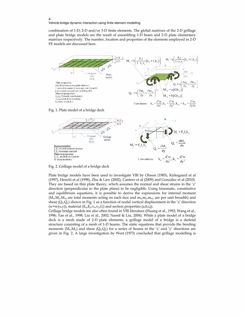
Fig. 1. Plate model of a bridge deck
Fig. 2. Grillage model of a bridge deck
Plate bridge models have been used to investigate VBI by Olsson (1985), Kirkegaard et al (1997), Henchi et al (1998), Zhu & Law (2002), Cantero et al (2009) and González et al (2010). They are based on thin plate theory, which assumes the normal and shear strains in the ‘z’ direction (perpendicular to the plate plane) to be negligible. Using kinematic, constitutive and equilibrium equations, it is possible to derive the expressions for internal moment (Mx,My,Mxy are total moments acting on each face and mx,my,mxy are per unit breadth) and shear (Qx,Qy) shown in Fig. 1 as a function of nodal vertical displacement in the ‘z’ direction (w=w(x,y)), material (Ex,Ey,vx,vy,G) and section properties (a,b,i,j). Grillage bridge models are also often found in VBI literature (Huang et al., 1992; Wang et al., 1996; Tan et al., 1998; Liu et al., 2002; Nassif & Liu, 2004). While a plate model of a bridge deck is a mesh made of 2-D plate elements, a grillage model of a bridge is a skeletal structure consisting of a mesh of 1-D beams. The static equations that provide the bending moments (Mx,My) and shear (Qx,Qy) for a series of beams in the ‘x’ and ‘y’ directions are given in Fig. 2. A large investigation by West (1973) concluded that grillage modelling is

5 Vehicle-bridge dynamic interaction using finite element modelling
very well suited for analysis of slab and beam-and-slab bridge decks and it has obvious advantages regarding simplicity, accuracy, computational time and ease to interpretate the results. It must be noted that there are a number of inaccuracies associated to grillage modelling (OBrien & Keogh, 1999). I.e., the diagram of internal forces is discontinuous at the grillage nodes and it is difficult to ensure the same twisting curvature in two perpendicular directions (kxy = kyx), although these limitations can be greatly reduced by the use of a fine mesh. Therefore, the influence of curvature in the direction perpendicular to the moment being sought (products vxkx and vyky in Equations of bending moment in Fig. 1) is ignored in grillage calculations, but the low value of Poisson’s ratio and the fact that this effect is ignored in both directions reduces the implications of this inconsistency. Finally, the influence of the twisting moment is neglected on the calculation of shear, which may be significant in the case of very high skew bridges. 2.2 Guidelines for Deck Modeling The properties of the 1-D beam elements of a grillage model or the 2-D elements of a plate model will depend of the type of deck cross-section being modelled: a solid slab, a voided slab, a beam-and-slab, or a cellular section, with or without edge cantilevers. When modelling a bridge deck using a plate FE model, OBrien & Keogh (1999) recommend to: (a) use elements as regularly shaped as possible. In the case of a quadrilateral element, one dimension should not be larger than twice the other dimension; (b) avoid mesh discontinuities (i.e., in transitions from a coarse mesh to a fine mesh all nodes should be connected); and (c) place element nodes at bearings and use elastic springs if compressibility of bearings or soil was significant. It must also be noted there are inaccuracies associated to the calculation of shear near supports which can result in very high and unrealistic values. The idealisation of a uniform solid slab deck as in Fig. 3 by a plate FE model is straightforward, i.e., the plate elements are given the same depth and material properties as the original slab. If using a grillage to model a solid slab deck, each grillage beam element (longitudinal or transverse) must have the properties (second moment of area and torsional constants) that resemble the longitudinal and transverse bending and twisting behaviour of the portion of the bridge being represented. By comparison of equations in Figs. 1 and 2, and neglecting the terms vyky and vxkx, the second moments of area for the grillage beams in the ‘x’ and ‘y’ directions that imitate the behaviour of a thin plate of width a, length b and depth d are given by:
≈xx y
iI = a ai
1 - v v; ≈y
x y
iI = b bi
1 - v v (3)
where i is the second moment of area per unit breadth of a thin plate or d3/12. The torsional constants of the beams in the longitudinal and transverse directions will be given by:
xJ = aj ; yJ = bj (4)
where j is the torsional constant per unit breadth of a slab or d3/6. Hambly (1991) provides the following recommendations to decide on the number of beams and location of nodes for
6 Vehicle-bridge dynamic interaction using finite element modelling
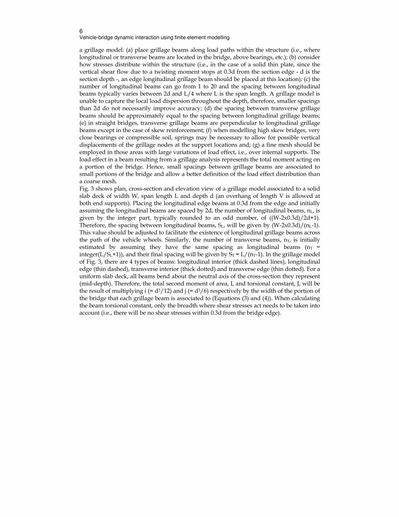
a grillage model: (a) place grillage beams along load paths within the structure (i.e., where longitudinal or transverse beams are located in the bridge, above bearings, etc.); (b) consider how stresses distribute within the structure (i.e., in the case of a solid thin plate, since the vertical shear flow due to a twisting moment stops at 0.3d from the section edge - d is the section depth -, an edge longitudinal grillage beam should be placed at this location); (c) the number of longitudinal beams can go from 1 to 20 and the spacing between longitudinal beams typically varies between 2d and L/4 where L is the span length. A grillage model is unable to capture the local load dispersion throughout the depth, therefore, smaller spacings than 2d do not necessarily improve accuracy; (d) the spacing between transverse grillage beams should be approximately equal to the spacing between longitudinal grillage beams; (e) in straight bridges, transverse grillage beams are perpendicular to longitudinal grillage beams except in the case of skew reinforcement; (f) when modelling high skew bridges, very close bearings or compressible soil, springs may be necessary to allow for possible vertical displacements of the grillage nodes at the support locations and; (g) a fine mesh should be employed in those areas with large variations of load effect, i.e., over internal supports. The load effect in a beam resulting from a grillage analysis represents the total moment acting on a portion of the bridge. Hence, small spacings between grillage beams are associated to small portions of the bridge and allow a better definition of the load effect distribution than a coarse mesh. Fig. 3 shows plan, cross-section and elevation view of a grillage model associated to a solid slab deck of width W, span length L and depth d (an overhang of length V is allowed at both end supports). Placing the longitudinal edge beams at 0.3d from the edge and initially assuming the longitudinal beams are spaced by 2d, the number of longitudinal beams, nL, is given by the integer part, typically rounded to an odd number, of ((W-2x0.3d)/2d+1). Therefore, the spacing between longitudinal beams, SL, will be given by (W-2x0.3d)/(nL-1). This value should be adjusted to facilitate the existence of longitudinal grillage beams across the path of the vehicle wheels. Similarly, the number of transverse beams, nT, is initially estimated by assuming they have the same spacing as longitudinal beams (nT = integer(L/SL+1)), and their final spacing will be given by ST = L/(nT-1). In the grillage model of Fig. 3, there are 4 types of beams: longitudinal interior (thick dashed lines), longitudinal edge (thin dashed), transverse interior (thick dotted) and transverse edge (thin dotted). For a uniform slab deck, all beams bend about the neutral axis of the cross-section they represent (mid-depth). Therefore, the total second moment of area, I, and torsional constant, J, will be the result of multiplying i (= d3/12) and j (= d3/6) respectively by the width of the portion of the bridge that each grillage beam is associated to (Equations (3) and (4)). When calculating the beam torsional constant, only the breadth where shear stresses act needs to be taken into account (i.e., there will be no shear stresses within 0.3d from the bridge edge).
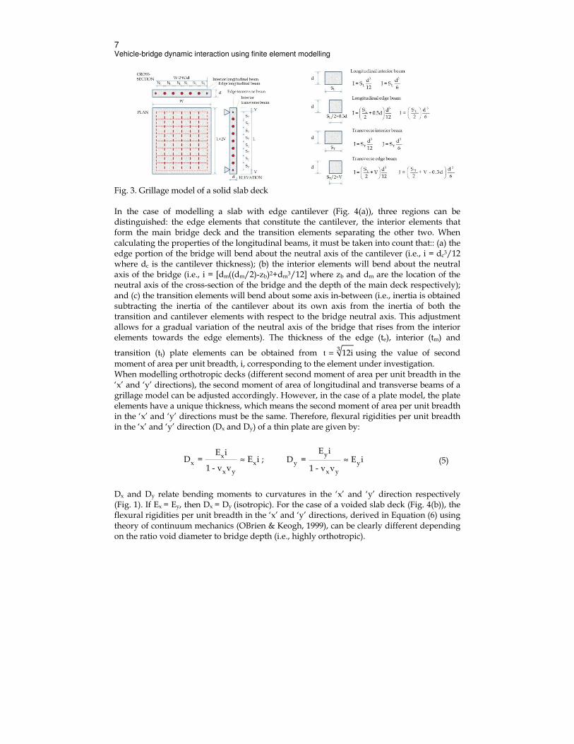
7 Vehicle-bridge dynamic interaction using finite element modelling
Fig. 3. Grillage model of a solid slab deck In the case of modelling a slab with edge cantilever (Fig. 4(a)), three regions can be distinguished: the edge elements that constitute the cantilever, the interior elements that form the main bridge deck and the transition elements separating the other two. When calculating the properties of the longitudinal beams, it must be taken into count that:: (a) the edge portion of the bridge will bend about the neutral axis of the cantilever (i.e., i = dc3/12 where dc is the cantilever thickness); (b) the interior elements will bend about the neutral axis of the bridge (i.e., i = [dm((dm/2)-zb)2+dm3/12] where zb and dm are the location of the neutral axis of the cross-section of the bridge and the depth of the main deck respectively); and (c) the transition elements will bend about some axis in-between (i.e., inertia is obtained subtracting the inertia of the cantilever about its own axis from the inertia of both the transition and cantilever elements with respect to the bridge neutral axis. This adjustment allows for a gradual variation of the neutral axis of the bridge that rises from the interior elements towards the edge elements). The thickness of the edge (te), interior (tm) and
transition (tt) plate elements can be obtained from t =3 12i using the value of second
moment of area per unit breadth, i, corresponding to the element under investigation. When modelling orthotropic decks (different second moment of area per unit breadth in the ‘x’ and ‘y’ directions), the second moment of area of longitudinal and transverse beams of a grillage model can be adjusted accordingly. However, in the case of a plate model, the plate elements have a unique thickness, which means the second moment of area per unit breadth in the ‘x’ and ‘y’ directions must be the same. Therefore, flexural rigidities per unit breadth in the ‘x’ and ‘y’ direction (Dx and Dy) of a thin plate are given by:
≈xx x
x y
E iD = E i
1 - v v; ≈
yy y
x y
E iD = E i
1 - v v (5)
Dx and Dy relate bending moments to curvatures in the ‘x’ and ‘y’ direction respectively (Fig. 1). If Ex = Ey, then Dx = Dy (isotropic). For the case of a voided slab deck (Fig. 4(b)), the flexural rigidities per unit breadth in the ‘x’ and ‘y’ directions, derived in Equation (6) using theory of continuum mechanics (OBrien & Keogh, 1999), can be clearly different depending on the ratio void diameter to bridge depth (i.e., highly orthotropic).

8 Vehicle-bridge dynamic interaction using finite element modelling
−
43v
xv
ddD = E
12 64s ;
4
1 0.95
−
3v
y
Ed dD =
d12 (6)
where E is the modulus of elasticity, d is the full depth of the voided slab, dv is the void diameter and sv is the distance between void centres. In order to be able to imitate the response of an orthotropic deck as closely as possible, the flexural rigidities of a plate FE model (Equation (5)) must be adjusted to match those in the original voided slab deck
(Equation (6)). For this purpose, two different modulus of elasticity are assumed, % xE and
%yE . Then, by doing %
xE = E , it is possible to obtain the value of the plate thickness replacing
the flexural rigidity of the original bridge in the ‘x’ direction (from Equation (6)) into
Equation (5), i.e., 3t = xD E . Similarly, the modulus of elasticity in the ‘y’ direction, % yE , is
adjusted to give the correct Dy (from Equation (6)) through %3
y yyE = D i = 12D t .
(a) (b)
Fig. 4. Grillage and plate FE models: (a) Slab with edge cantilever; (b) Voided slab When using a grillage to model a beam-and-slab deck, the girders and diaphragms of the deck are associated to longitudinal and transverse grillage beams respectively. Additional transverse grillage beams representing only slab will be necessary to cover for the entire bridge span. When calculating the properties of the longitudinal grillage beams, it must be taken into account that the portion of the deck being represented will bend about its own axis (and not about the neutral axis of the entire bridge cross-section) due to the poor load transfer of this type of construction. The torsional constant of a longitudinal grillage beam will be equal to the torsional constant of the bridge beam plus the torsional constant of the thin slab. When transverse grillage beams are not placed at the location of diaphragm beams, and they only represent slab, they will bend about the neutral axis of the slab and their torsional constant will be equal to the torsional constant of a thin slab. Therefore, in the case of a composite section made of different materials for beam and slab, properties will be obtained using an equivalent area in one of the two materials, adjusting the width of the other material based on the modular ratio. Alternatively, a beam-and-slab bridge deck can be modelled using a combination of 1-D beams and 2-D plates. The guard rails, longitudinal and transverse beams in the bridge will be idealised with beam elements while the deck will be modelled with plate elements (Chompooming & Yener, 1995; Kim et al., 2005; González et al., 2008a).

9 Vehicle-bridge dynamic interaction using finite element modelling
In the case of using a grillage to model a cellular deck, a longitudinal grillage beam can be placed at the location of each web making the cross-section. These grillage beams will bend about the neutral axis of the full section. The properties of edge longitudinal grillage members representing edge webs must take into account the possible contribution of edge cantilevers to torsion and bending stiffness. The sum of the torsional constants of all grillage longitudinal beams will be equal to the sum of the torsional constants of the individual cells (i.e., a closed section) plus the torsional constants of the edge cantilevers (i.e., a thin slab). Caution must be placed upon the determination of the area of the transverse grillage beams, which should be reduced to allow for transverse shear distortion, typical of cellular sections. Models of bridges with cables attached to the deck can be found in Wang & Huang (1992), Chatterjee et al (1994a), Guo & Xu (2001), Xu & Guo (2003) and Chan et al (2003).
3. The Vehicle
While the equations of motion of the bridge are obtained using the FE package, there are three alternative methods to derive the equations of motion of the vehicle: (a) imposing equilibrium of all forces and moments acting on the vehicle and expressing them in terms of their DOFs (Hwang & Nowak, 1991; Kirkegaard et al., 1997; Tan el al., 1998; Cantero et al., 2010), (b) using the principle of virtual work (Fafard et al., 1997) or a Lagrange formulation (Henchi et al., 1998), and (c) applying the code of an available FEM package. The equations of equilibrium deal with vectors (forces) and they can be applied to relatively simple vehicle models, while an energy approach has the advantage of dealing with scalar amounts (i.e., contribution to virtual work) that can be added algebraically and are more suitable for deriving the equations of complex vehicle models. Similarly to the bridge, the equations of motion of a vehicle can be expressed in matrix form as:
&& &v v v v v v v[M ]{w } + [C ]{w } + [K ]{w } = {f } (7)
where [Mv], [Cv] and [Kv] are global mass, damping and stiffness matrices of the vehicle
respectively, v{w } , & v{w } and && v{w }
are the vectors of global coordinates, their velocities
and accelerations respectively, and {fv} is the vector of forces acting on the vehicle at time t. The modes of vibration of the theoretical model should resemble the body pitch/bounce and axle hop/roll motions of the true vehicle. Body oscillations are related to the stiffness of suspensions and sprung mass (vehicle body) and they have frequencies between 1 and 3 Hz for a heavy truck and between 2 and 5 Hz for a light truck. Axle oscillations are mainly related to the unsprung masses (wheels and axles) and have higher frequencies, in a range from 8 Hz to 15 Hz. In the presence of simultaneous vehicle presence, frequency matching and resonance effects on the bridge response are unlikely. But in the case of a single truck, Cantieni (1983) has measured average dynamic increments on bridges with normal pavement conditions of 30-40% (maximum of 70%) when their first natural frequency felt within the range 2 to 5 Hz, that decreased to an average dynamic increment between 10 and 20% when the natural frequency felt outside that frequency range. Green et al (1995) analyse the decrease in bridge response when the vehicles are equipped with air-suspensions compared to steel suspensions due to the low dynamic forces they apply to the bridge.
10 Vehicle-bridge dynamic interaction using finite element modelling
3.1 Types of FE Models for Vehicles
There is a wide range of sprung vehicle models used in VBI investigations. Planar vehicle models have been found to provide a reasonable bridge response for ratios bridge width to vehicle width greater than 5 (Moghimi & Ronagh, 2008a). A single-DOF model can be used for a preliminary study of the tyre forces at low frequencies due to sprung mass bouncing and pitching motion (Chatterjee et al., 1994b; Green & Cebon, 1997) and a two-DOF model (i.e., a quarter-car) can be employed to analyse main frequencies corresponding to body-bounce and axle hop modes (Green & Cebon, 1994; Chompooming & Yener, 1995; Yang & Fonder, 1996; Cebon, 1999). If the influence of axle spacing was investigated, then a rigid walking beam (Hwang & Nowak, 1991; Green & Cebon, 1994; Chompooming & Yener, 1995) or articulated multi-DOF model (Veletsos & Huang, 1970; Hwang & Nowak, 1991; Green et al., 1995; Harris et al., 2007) will become necessary. The vehicle model can be extended to three dimensions to allow for roll and twisting motions. Most of these spatial models consist of an assemblage of 1-D elements, but they can also be made of 2-D and 3-D FEs for a detailed representation of the vehicle aerodynamic forces and deformations (Kwasniewski et al., 2006). However, it seems unlikely such a degree of sophistication could affect the bridge response significantly. So, spatial FE vehicle models are typically composed of mass, spring, bar and rigid elements that are combined to model tyre, suspension, axle/body masses and connections between them. The equations of motion of a spatial vehicle model can be established for rigid (Tan et al., 1998; Zhu & Law, 2002; Kim et al., 2005) or articulated configurations (EIMadany, 1988; Fafard et al., 1997; Kirkegaard et al., 1997; Nassif & Liu, 2004; Cantero et al., 2010). In the latter, equations of motion can be formulated for the tractor and trailer separately, and the DOFs of both parts can be related through a geometric condition that takes into account the hinge location. A series of lumped masses are employed to represent axles, tractor and trailer body. The body masses are connected to the frame by rigid elements, and the frame is connected to the axles by spring-dashpot systems that model the response of the suspension. Each axle is typically represented as a rigid bar with lumped masses at both ends that correspond to the wheel, axle bar, brakes and suspension masses (Alternatively, the axle mass can be assumed to be concentrated at the local centre of gravity of the rigid bar connecting both wheels with two DOFs: vertical displacement and rotation about the longitudinal axis). Then, the lumped mass at each wheel is connected to the road surface by a spring-dashpot system simulating the response of the tyre. Fig. 5 illustrates the forces acting on the tractor and trailer masses of an articulated vehicle travelling at constant speed. Equations of motion for a vehicle braking or accelerating can be found in Law & Zhu (2005) and Ju & Lin (2007). The system of time-varying forces acting on each lumped mass consists of inertial forces
(i.e., &&i- j i- jm w ), gravity forces (mi-jg), suspension forces (fS,i-j) and tyre forces (fT,i-j).
Equilibrium of vertical forces acting on the sprung mass of the tractor and equilibrium of moments of all forces about a ‘y’ axis going through its centroid (Fig. 5(a)) lead to Equations (8) and (9) respectively.
p
( ) S,i-left S,i-rights s Hi=1
m w g (f f ) f 0∑ ∑→ − + + + =&&zF = 0 (8)

11 Vehicle-bridge dynamic interaction using finite element modelling
where fH is the interaction force at the hinge and p is the number of axles supporting the sprung mass.
p
y S,i-right S,i-lefty y i H Hi=1
= 0 I θ (f f )x f x 0∑ ∑→ − + − =&&M (9)
where xi is the distance from axle i to the centroid of the sprung mass, and it can be positive (to the right of the centroid) or negative (to the left of the centroid). Similar equations of equilibrium can be obtained for the sprung mass of the trailer. From equilibrium of moments of all forces acting on the body mass about an ‘x’ axis going through its centroid (Fig. 5(b)), it is possible to obtain:
∑ ∑ ∑→ &&p p
x S,i-left i-left S,i -right i-rightx xi=1 i=1
M = 0 I θ + f a f a- = 0 (10)
(a) (b)
Fig. 5. Lumped mass vehicle model: (a) Forces acting on tractor and trailer sprung masses (side view), (b) Forces acting on the sprung and unsprung masses (front view) Wheel, axle and suspension mass are assumed to be concentrated at both ends of an axle i (mi-left and mi-right), and equilibrium at these lumped masses is given by Equation (11). Identical equations can be obtained for the unsprung masses of the trailer.
∑ →zF =0
i-righti i-left
( )i-left i-left S,i-left S,i-right T,i-lefti i
i i-right i-lefti-right i-right S,i-right S,i-left T,i-right
i i
bd -bm w g f f f 0
d d
d -b bm (w g) f f f 0
d d
− − − + =
− − − + =
&&
&&
; i = 1,…,p (11)
The two equations of equilibrium of vertical forces of the tractor (Equation (8)) and trailer body masses can be combined into one by cancelling out fH. Therefore, the suspension and tyre forces can be expressed as a function of the DOFs of the vertical displacement of the unsprung and sprung masses. Tyre forces can be defined by viscous damping elements (proportional to the damping constant and the relative change in velocity between the two

12 Vehicle-bridge dynamic interaction using finite element modelling
end points of the damper), and spring elements (proportional to the stiffness constant and the relative change in displacement between the two end points of the spring) as given in Equation (12) for the wheel forces in the left side.
( ) ( )& & &T,i-left T,i -left i-left i -left i -left T,i -left i-left i-left i -leftf = k w + u - r + c w + u - r (12) where ui-left and ri-left represent the bridge displacement and the height of the road irregularities respectively under the left wheel of axle i at a specified point in time. ui-j is related to the nodal displacements and rotations {wb}(e) of the bridge element where the wheel i-j is located through the displacement interpolation functions {N(x, y)} of the element.
The values of {N(x, y)} are a function of the coordinates (x, y) of the wheel contact point with
respect to the coordinates of the bridge element.
(e)Ti- j bu = {N(x, y)} {w } (13)
In Figure 5(b), suspension systems have also been defined by a viscous damping element in parallel with a spring element. In this case of linear suspension elements, the forces fS are given by Equation (14) for the suspension forces in the left side of the vehicle.
( )( ) ( )( )y x y xθ θ θ θ+ +& && &S,i-left S,i-left s i i-left i-left i-left S,i-left s i i-left i-left i -leftf = k w + x + a b - w + c w + x + a b - w
(14) The equations of tractor and trailer are not independent, as a compatibility condition can be defined between both rigid bodies rotating about the hinge (also known as fifth wheel point). Therefore, the number of DOFs of the system can be reduced by considering the following relationship between the displacements of the centroids of tractor and trailer:
y yθ θ%% %s s H Hw = w + x + x (15) All equations of equilibrium can be expressed as a function of the vertical displacements of the wheels ( )% % % %1-left 1-right p-left p-right 1-left 1-right p-left p-rightw , w , ...., w , w , w , w , ...., w , w , the three DOFs of
the tractor (ws,θx,θy) and the two DOFs of the trailer ( % %x yθ , θ ), by replacing Equations (12),
(14) and (15) into the equations of equilibrium of the lumped masses. The equations can be expressed in a matrix form which will lead to the mass, stiffness and damping matrices of the vehicle (Equation (7)). The coefficients of these matrixes can be found in Cantero et al (2010) for an arbitrary number of tractor and trailer axles. The forcing vector {fv} will be a combination of tyre properties (stiffness/damping) and height of the road/bridge profile. Values for parameters of suspension and tyre systems are available in the literature (Wong, 1993; Kirkegaard et al., 1997; Fu & Cebon, 2002; Harris et al., 2007). In the case of a 5-axle articulated truck, typical magnitudes are 7000 kg for a tractor sprung mass, 700 kg for a steer axle, 1000 kg for a drive axle, 800 kg each trailer axle, tyre stiffness of 735x103 kN/m and damping of 3x10³ kNs/m, suspension stiffness of 300x103 kN/m for a steer axle, 500x103 and 1000x103 kN/m for a drive axle if air- and steel-suspension respectively, 400x103 and

13 Vehicle-bridge dynamic interaction using finite element modelling
1250x103 kN/m for a trailer axle if air- and steel-suspension respectively, and suspension viscous damping of 3x10³ kNs/m. The general form of the equations of motion described in this section is only valid for linear tyre and suspension systems and it needs to be adapted to introduce different degrees of complexity within the vehicle behaviour, such as tyre or suspension non-linearities. Green & Cebon (1997) propose the following equation that facilitates the incorporation of non-linear elements:
[ ]{ }&&v v v S v TM w = [S ]{f } + [T ]{f } + {G} (16)
where {fS} and {fT} are vectors of suspension and tyre forces respectively, [Sv] and [Tv] are constant transformation matrices relating the suspension and tyre forces respectively to the
global coordinates of the vehicle, and { }G is the vector of gravitational forces applied to the
vehicle. The relationship between Equations (7) and (16) is given by {fv} = [Tv][KT]{v}
[ ]{ }= &TC v where [KT] and [CT] are stiffness and damping matrices respectively for tyre
elements and {v} is the height of road irregularities (or road irregularities plus bridge deflections), [Cv]=[Sv]{CS][Sv]T+[Tv][CT][Tv]T and [Kv]=[Sv][KS][Sv]T+[Tv][KT][Tv]T where [KS] and [CS] are stiffness and damping matrices respectively for suspension elements.
4. The Road
The road profile can be measured or simulated theoretically. When simulating a profile r(x), it can be generated from power spectral density functions as a random stochastic process:
N
d k k ii=1
r(x)= 2G (n )∆ncos(2πn x-θ )∑ (17)
where Gd(nk) is power spectral density function in m2/cycle/m; nk is the wave number (cycle/m); θi is a random number uniformly distributed from 0 to 2π; ∆n is the frequency interval (∆n = (nmax–nmin)/N where nmax and nmin are the upper and lower cut-off frequencies respectively); N is the total number of waves used to construct the road surface and x is the longitudinal location for which the road height is being sought. The road class is based on the roughness coefficient a (m3/cycle), which is related to the amplitude of the road irregularities, and determines Gd(nk) (Gd(nk) is equal to a/(2πnk)2). ISO standards specify ‘A’ (a < 2x10⁻⁶), ‘B’ (2x10⁻⁶ ≤ a < 8x10⁻⁶), ‘C’ (8x10⁻⁶ ≤ a < 32x10-6), ‘D’ (32x10-6 ≤ a < 128x10-6) and other poorer road classes depending on the range of values where a is located (ISO 8608, 1995). For a given roughness coefficient, different road profiles can be obtained varying the random phase angles θi. When using two parallel tracks of an isotropic surface, a coherence function needs to be employed to produce a second random profile correlated with the first profile (Cebon & Newland, 1983; Cebon, 1999; Nassif & Liu, 2004). The coherence function guarantees good and poor correlation between two parallel tracks for long and short wavelengths respectively. The contact between the bridge and the vehicle is typically assumed to be at a single point rather than the area corresponding to the tyre patch. Therefore, the lengths of randomly generated road profile are passed through a
14 Vehicle-bridge dynamic interaction using finite element modelling
moving average filter to simulate the envelope of short wavelength disturbances by the tyre contact patch (i.e., 0.2 m). The magnitude of the bridge response depends strongly not only on the general unevenness of the bridge surface, but also on the velocity of the vehicles (González et al., 2010), the condition of the road leading to the bridge, and the effects of occasional large irregularities such as potholes, misalignments at the abutments or expansion joints that are often found on the bridge approach. Chompooming & Yener (1995) show how certain combinations of bumps and vehicle speed can originate a high dynamic excitation of the bridge.
5. Vehicle-Bridge Interaction Algorithms
When analysing the VBI problem, two sets of differential equations of motion can be established: one set defining the DOFs of the bridge (Equation (1)) and another set for the DOFs of the vehicle (Equation (7)). It is necessary to solve both subsystems while ensuring compatibility at the contact points (i.e., displacements of the bridge and the vehicle being the same at the contact point of the wheel with the roadway). The algorithms to carry out this calculation can be classified in two main groups: (a) those based on an uncoupled iterative procedure where equations of motion of bridge and vehicle are solved separately and equilibrium between both subsystems and geometric compatibility conditions are found through an iterative process (Veletsos & Huang, 1970; Green et al., 1995; Hwang & Nowak, 1991; Huang et al., 1992; Chatterjee et al., 1994b; Wang et al., 1996; Yang & Fonder, 1996; Green & Cebon, 1997; Zhu & Law, 2002; Cantero et al., 2009), and (b) those based on the solution of the coupled system, i.e., there is a unique matrix for the system that is formed by eliminating the interaction forces appearing in the equations of motion of bridge and vehicle, and updated at each point in time (Olsson, 1985; Yang & Lin, 1995; Yang & Yau 1997; Henchi et al., 1998; Yang et al., 1999, 2004a; Kim et al., 2005; Cai et al., 2007; Deng & Cai, 2010; Moghimi & Ronagh, 2008a). The use of Lagrange multipliers can also be found in the solution of VBI problems (Cifuentes, 1989; Baumgärtner, 1999; González et al., 2008a). A step-by-step integration method must be adopted to solve the uncoupled or coupled differential equations of motion of the system. These numerical methods break the time down into a number of steps, ∆t, and calculate the solution w(t+∆t) from w(t) based on assumed approximations for the derivatives that appear in the differential equations. They are different from methods for single-DOF systems because most FE models with lots of DOFs poorly idealise the response of the higher modes, and the integration method should have optimal dissipation properties for the removal of those non-reliable high frequency contributions. Fourth-order Runge-Kutta is a popular integration method in the solution of large multi-DOF VBI systems (Frýba 1972; Huang et al., 1992; Wang & Huang, 1992; Cantero et al., 2009; Deng & Cai, 2010). Acceleration is expressed as a function of the other lower derivatives and a change of variable transforms the second order equation of motion into two first order equations (Equation (18)). Then, the recurrence formulae of fourth-order Runge-Kutta is employed to approximate the derivatives according to a weighted average of four estimates of the slope in the interval ∆t.
&{Z} = {w} ; 1{{f} [ ]{ } }
−− −&{Z} = [M] C Z [K]{w} (18)

15 Vehicle-bridge dynamic interaction using finite element modelling
Fourth-order Runge-Kutta is easy to implement, however, it is conditionally stable and it requires evaluating several functions per time step which can be time-consuming. For these reasons, some authors prefer implicit unconditionally stable integration methods such as Newmark-β (Olsson, 1985; Hwang & Nowak, 1991; Chompooming & Yener, 1992; Yang & Fonder, 1996; Fafard et al., 1997; Yang & Yau, 1997; Zhu & Law, 2002; Kim et al., 2005) or Wilson-θ (Tan et al., 1998; Nassif & Liu, 2004). The Newmark family of integration methods is based on a truncation of Taylor’s series that assumes a linear variation of acceleration from time t to time (t+∆t) (a constant acceleration with parameters β = 0.25 and γ = 0.5 is typically used to avoid instability problems). Wilson-θ is a modified version of the Newmark method, where acceleration is assumed to vary linearly from time t to time (t+θ∆t) (θ ≥ 1.37, usually 1.4). After the conditions at time (t+θ∆t) are known, they are referred back to produce a solution at time (t+∆t). Clough & Penzien (1993) recommend a time step ∆t ≤ 1/(10fmax) where fmax is the maximum frequency of the system to ensure convergence. Typical values of ∆t lie between 0.001 and 0.0001 s. In the case of non-linear equations of motion, i.e., the non-linear relationship between the force and nodal displacements in leaf-spring suspensions, an iterative procedure needs to be implemented for each point in time (Veletsos & Huang, 1970; Hwang & Nowak, 1991; Wang & Huang, 1992; Chatterjee et al., 1994a,b; Tan et al., 1998; Nassif & Liu, 2004). The initial values of the force and nodal displacement of the suspension are assumed to be those of the preceding time step. However, once the equations of the system are solved for the current time, the suspension nodal displacement will be somehow different from the value in the previous time step and the associated suspension force may change with respect to the assumed initial value. The calculations need to be repeated with the updated value of suspension force, and treated in an iterative procedure until reaching an acceptable tolerance that indicates negligible difference between displacements/forces of two successive iterations.
5.1 Algorithms based on an Uncoupled Iterative Procedure
These algorithms treat the equations of motion of the vehicle and the bridge as two subsystems and solve them separately using a direct integration scheme. The compatibility conditions and equilibrium equations at the interface between the vehicle tyres and bridge deck are satisfied by an iterative procedure. The basic idea behind this procedure consists of assuming some initial displacements for the contact points, which can be replaced in the equations of motion of the vehicle to obtain the interaction forces. Then, these interaction forces are employed in the equations of motions of the bridge to obtain the bridge displacements that will represent improved estimates of the initial displacements assumed for the contact points. The process is repeated until differences in two successive iterations are sufficiently small. These algorithms typically employ implicit schemes of integration such as Newmark-β or Wilson-θ methods to solve each subsystem and to achieve convergence after a number of iterations. The time step ∆t here is larger than in the coupled solution, although the convergence rate may be slow. One possible algorithm within the group of iterative procedures is illustrated in Fig. 6. The vehicle and the bridge interact through the tyre forces imposed on the bridge deck. The profile, v(x,t), that is used to excite the vehicle is the sum of the original road profile (r(x)) and the deflection of the bridge (wb(x,t)) (In the first step of the iterative procedure, no bridge displacements have been calculated yet and v(x,t) can be taken to be r(x)). The

16 Vehicle-bridge dynamic interaction using finite element modelling
interaction forces (tyre forces {fT}) are obtained solving for the DOFs of Equation (7) and replacing into Equation (12). These interaction forces are converted to equivalent bridge forces acting on the bridge nodes in the vicinity of the contact point using a location matrix ({fb}=[L]{fT} where [L] is a location matrix that relates the tire forces to the DOFs of the bridge). Then, {fb} is employed to obtain a new set of displacements wb(x,t) using Equation (1). This procedure is repeated for a number of iterations at each time step until some convergence criteria is met (i.e., difference between the bridge deflection wb(x,t) of two successive iterations being sufficiently small). Green & Cebon (1997) suggest to average bridge displacements in two successive iterations to facilitate convergence which they define as the relative difference in displacement of two successive iterations with respect to the maximum bridge deflection to be smaller than 2%. At that point, the vehicle is moved forward and the iterative procedure is repeated for the new location of the forces on the bridge.
Fig. 6. VBI iterative procedure Cantero et al (2009) suggest an alternative iterative procedure, where rather than calculating the final interaction forces at each time step, an initial estimate of the entire force history {fT}(1) is obtained using Equations (7) and (12) with only the road profile r(x) (=v(x,t)(1)) as excitation source. Equation (1) is employed to calculate the bridge deflections, wb(x,t)(1), due to the equivalent nodal forces {fb}(1) derived from {fT}(1). The bridge deflection wb(x,t)(1) is then added to the road profile r(x) to form v(x,t)(2), and a new estimated of the force history {fT}(2) is obtained using the equations of motion of the vehicle and the profile v(x,t)(2) as excitation source. These time-varying forces {fT}(2) are converted into bridge nodal forces {fb}(2) that will result into a new bridge deflection history wb(x,t)(2) using Equation (1). The process is repeated until convergence is achieved.

17 Vehicle-bridge dynamic interaction using finite element modelling
While the previous algorithms have been formulated in the time domain, Green & Cebon (1994,1997), Green et al (1995) and Henchi et al (1997) propose to solve the uncoupled system of equations in the frequency domain. The equations of motion are solved by convolution of modal impulse response functions and modal excitation forces through the FFT, and application of modal superposition. It must be noted that many DOFs are involved in the FE model of the bridge subsystem, but only the first modes of vibration make a significant contribution to the dynamic response of a VBI system. Therefore, the modal superposition method (MSM) is typically employed to solve the equations of motion of the bridge which reduces the computation effort considerably (Clough & Penzien, 1993). The basis of the MSM is the transformation of the original system of coupled equations (Matrixes in Equation (1) with non-zero off-diagonal terms) into a smaller set of uncoupled independent modal coordinate equations (i.e., zero off-diagonal terms). The total dynamic response will be obtained by superposition of the response obtained for each modal coordinate. The displacement vector of the bridge {wb} can be expressed as a function of the modal coordinates {qb} as follows:
b b b{w }=[ ]{q }Φ (19)
where [Фb]=[{Ф1}{Ф2}…{Фm}] is the normalized modal shape matrix containing a number m of mode shapes. The mode shapes {Фi}
and frequencies associated to these mode shapes ωi
can be found using eigenvalue analysis:
{ }[ ] [ ] { } 2
b i b iK - ω M Φ = 0 (20)
Therefore [Фb]
is normalized such that:
T
b b b[Φ ] [M ][Φ ]=[I]
; T 2
b b b b[Φ ] [K ][Φ ]=[ω ] (21)
where [ωb2] is a diagonal matrix containing the squares of the natural frequencies. Equation (1) can be written in modal coordinates as:
[ ][ ]{ } [ ][ ]{ } [ ][ ]{ }Φ Φ Φ&& &b b b b b b b b b bM q + C q + K q = {f } (22)
Assuming that the damping matrix [Cb] satisfies modal orthogonality conditions (e.g., Rayleigh damping) and premultiplying both sides of the equation by [Фb]T, the following simplified system with m differential equations in modal coordinates results:
2 T
b b b b b b b b{q }+2[ξ ][ω ]{q }+[ω ]{q }=[ ] {f }Φ&& & (23)
where [ξb] and [ωb] are modal damping and modal frequency matrixes of the bridge respectively and their size is related to the number of modes of vibration considered; {qb}
is
the modal coordinate vector and a dot means derivative with respect to time. Modal Equation (23) is a series of independent single-DOF equations, one for each mode of

18 Vehicle-bridge dynamic interaction using finite element modelling
vibration, that can be solved by Newmark, Wilson-θ, Runge-Kutta or a piece-wise interpolation integration technique. The total response is obtained from the superposition of the individual modal solutions (Equation (19)). In some cases, the modal equations can become coupled (i.e., damping matrix of the system not being diagonal after modal transformation) and the modal equations will need to be solved using a step-by-step integration method simultaneously rather than individually, but the reduction of the original number of equations where all DOFs were considered to a number m of modal equations will still be computationally advantageous. If the number of DOFs of the vehicle was considerably large, the MSM can also be applied to the equations of motion of the vehicle subsystem (Equation (7)).
5.2 Algorithms based on the Solution of the Coupled System
These algorithms are based on the solution of a unique system matrix at each point in time. The system matrix changes as the vehicle moves and its time-dependent properties can be derived using the principle of virtual work. These algorithms commonly use a step-by-step integration scheme such as Newmark-β (Kim et al., 2005) or fourth order Runge-Kutta (Deng & Cai, 2010) with a small time step ∆t to solve the system matrix at each point in time. This procedure can be carried without any iteration if linear elements are employed, but if non-linear elements, such as friction, were present in the model, iterations will be necessary regardless of the vehicle-bridge system being solved as two subsystems or as one. The vehicle-bridge equations can be combined to form the system given below:
b b b b-b b-v b b b-b b-v b b-r
v v v-b v v v-b v v b-r
[M ] [0] {w } [C +C ] [C ] {w } [K +K ] [K ] {w } {f }+ + =
[0] [M ] {w } [C ] [C ] {w } [K ] [K ] {w } {f } { }{ } { } { } { }
+
&& &
&& & G
(24) where {G} are gravity forces and [Cb-b], [Cb-v], [Cv-b], [Kb-b], [Kb-v], [Kv-b] and {fb-r} are time dependent matrixes/vectors that depend on the value and location of the interaction forces at each point in time. Equation (25) shows how MSM can be used to simplify the bridge subsystem of Equation (24).
T Tb bb b b b-b b b b-v
v v vv-b b v
2 T T Tbb b b-b b b b-v b b-r
vv-b b v b-r
{q } {q }[I] [0] 2[ξ ][ω ]+[ ] [C ][ ] [ ] [C ]+
[0] [M ] {w } {w }[C ][ ] [C ]
{q }[ω ]+[ ] [K ][ ] [ ] [K ] [ ] {f }+ =
{w }[K ][ ] [K ] {f } { }
{ } { }
{ } { }
Φ Φ Φ
Φ
Φ Φ Φ Φ
Φ +
&& &
&& &
G
(25)
The approach above is adopted by Deng & Cai (2010) and Henchi et al (1998) that combine DOFs of the bridge in the modal space and DOFs of the vehicle derived from a Lagrange formulation. Henchi et al (1998) use a central difference method to solve the coupled equations which finds computationally more efficient than an uncoupled approach solved using Newmark-β. However, some authors note some disadvantages of this method regarding computational effort as a result of properties of the vehicle and bridge matrixes such as symmetry being lost in the process, the need to update the coefficients matrices of

19 Vehicle-bridge dynamic interaction using finite element modelling
the system at every time step with new positions of the vehicle on the bridge, or to carry new calculations of coefficients if the vehicle or bridge model changed (Yang & Lin, 1995; Yang & Fonder, 1996; Kirkegaard et al., 1997). An alternative approach that leads to considerable savings in computational time is to implement the interaction on an element level rather than on a global level (Olsson, 1985; Yang & Lin, 1995; Yang & Yau, 1997; Yang et al., 1999). An interaction element is defined as that bridge element in contact with a vehicle wheel. Those bridge elements that are not directly under the action of vehicle wheels remain unaltered in the global matrixes of the system. The interaction element is characterised by two sets of equations: those of the bridge element and those of the moving vehicle above the bridge element. The DOFs of the moving vehicle can be solved in time domain using finite-difference equations of the Newmark type, and then, the DOFs of the vehicle that are not in direct contact with the bridge are eliminated and condensed to the DOFs of the associated bridge element via the method of dynamic condensation. The interaction element has the same number of DOFs as the original bridge element and it can be directly assembled with the other bridge elements into the global matrixes, while retaining properties that are lost when condensation takes place on a structure level.
5.3 Algorithms based on Lagrange Multipliers The system of equations (24) can be extended with a number of additional coordinates to maintain symmetry. The differential equations of motion of the vehicle-bridge system are formed by the equations of the bridge and vehicle which appear without overlapping in the system matrix, and a number of additional constraints that enforce the compatibility condition at the contact points of vehicle and bridge. An advantage of this approach is the ease to accommodate it to a standard FE package (to qualify, the software should have the capability for solving a transient dynamic response, and to allow for direct inputs into the system matrix) while a drawback is the number of additional rows and columns in the system matrix that may require a significant computational effort. Compatibility conditions between the vertical displacement uj(t) of each moving wheel j and the vertical displacement of the bridge at the contact point wb(xj,t), are established for any time t with the use of time-dependent functions (Aij(t) and Bij(t) which vary for each node i and load j at each instant t). These auxiliary functions produce a constraint consistent with the shape functions of the bridge elements and they facilitate to formulate the compatibility condition at the contact point of the wheel j as:
∑ ∑N N
j i j b,i i j b,ii=1 i=1
u (t) = A (t)w (t) + B (t)θ (t) ; j = 1,2, …p (26)
where wb,i(t) (=wb(xi,t)) and θi(t) are the displacements and rotations of the node i in the bridge FE model, and N and p are the total number of bridge nodes and moving wheels respectively. Aij(t) and Bij(t) can be completely defined prior to the simulation once the velocity of the moving loads, the approach length, the spacings between loads and the coordinates of the bridge nodes on the wheel path are known. For illustration purposes only, the shape of these functions for bridge beam elements with nodes numbered 5, 6 and 7 and moving load 1 is shown in Fig. 7 (The values of Bij(t) will depend on the distance between consecutive nodes, ∆x). They have zero value outside the interval between adjacent

20 Vehicle-bridge dynamic interaction using finite element modelling
nodes, and for the location of a vehicle wheel j over a bridge node i, Aij(t) and Bij(t) become 1 and 0 respectively, which satisfies uj(t)=wb,i(t). The numerical expression for these auxiliary functions can be found in Cifuentes (1989) and González et al (2008a).
(a) (b)
Fig. 7. Auxiliary Functions: (a) Aij(t), (b) Bij(t) (∆x=1) The vector of equivalent nodal forces {fb} composed of forces fi(t) and moments Mi(t) acting on a bridge node i at time t can also be expressed as a function of the p interaction forces using the auxiliary functions:
∑p
i i j j jj=1
f (t) = A (t)(R + G ) ; ∑p
i i j j jj=1
M (t) = B (t)(R + G ) ; i = 1,2, …N (27)
where Rj and Gj represent dynamic and static components respectively of the moving force j. The final system matrix is given in Equation (28) for a discretized beam bridge model with N nodes and p moving forces (Baumgärtner, 1999). The group of equations in the first row of the system matrix represents the motion of the bridge. The forcing term corresponding to this first row is expressed as a function of the auxiliary functions as defined by Equation (27). The second row assigns values of the auxiliary functions to scalar points ({s}) and it has a size equal to the number of bridge nodes in each wheel path multiplied by twice the number of wheels (Aij and Bij). The third and fourth rows of the system matrix represent the equations of motion of the vehicle. The equations of motion relating the DOFs of the wheel contact points (=p) to the interaction forces {Rj} are given in the third row while the equations of motion of the remaining DOFs of the vehicle are given in the fourth row. In the fifth row, the only terms that are not zero are those that impose the constraint condition between deflections of the moving wheels and the bridge (Equation (26)). When comparing the system matrix of Equation (28) to the one in Equation (24), it can be observed that the system matrix is larger, but it is not time dependent. Therefore, in Equation (24) the forcing vector contains only forces and the vector of unknowns contains only displacements while in Equation (28) these vectors contain both forces and displacements. This coupling between vectors requires an iteration procedure at each point in time until achieving convergence. Details of the implementation of this technique using a fully computerized approach where the bridge and vehicle models are built using NASTRAN are given by González (2010).

21 Vehicle-bridge dynamic interaction using finite element modelling
[ ][ ] +
2
b b2
dM K
dt
0 0 0 0
wb,1
… wb,N
Σs1j (Rj+Gj) …
ΣsNj(Rj+Gj)
0 [I] 0 0 0
s11 s12 … spN
A11(t) A12(t)
… ApN(t)
0 0
[ ] [ ][ ] + +
2
v v v2
d dM C K
dt dt [I]
u1 … up
= 0 … 0
0 0 0 {wv} {0}
0 0 [I] 0 0 R1
… Rp
Σs1iwb,i
…
Σspiwb,i
(28)
6. Conclusions
This chapter has reviewed the techniques used for simulating the response of a bridge to the passage of a road vehicle, from the initial stages of preparation of the FE models of bridge and vehicle to the implementation of the interaction between both. VBI simulations can be used to compare the performance of alternative bridge designs or retrofitting options when traversed by traffic and to identify those bridge solutions less prone to dynamic excitation. They can also be employed to quantify the increase in dynamic amplification due to a rougher profile or a deteriorated expansion joint. Other relevant topics in VBI research concern traffic properties, i.e., suspension and tyre types, speed, acceleration/deceleration, vehicle weights and configuration, frequency matching or multiple vehicle presence. A direct application of VBI modelling is related to the characterization of the total traffic load on a bridge. The traffic load model specified in the bridge design codes is a function of the bridge span length (or natural frequency), number of lanes or load effect, and it is necessarily conservative due to the uncertainties governing the bridge response to a critical traffic loading event prior to its construction. For instance, the critical traffic loading condition is likely to consist of vehicle configurations with very closely spaced axles, which generally tend to produce relative dynamic increments smaller than configurations with longer axle spacings. Additionally, in the case of long span bridges, the critical traffic loading condition consists of a traffic jam situation where vehicles travel at low speed and typically cause a minor dynamic excitation of the bridge. In the case of short-span bridges, the critical situation will be composed of a reduced number of vehicles travelling at highway speed that cause dynamic amplification factors very sensitive to the condition of the road profile before and on the bridge. Thus, bridge codes recommend higher dynamic allowances for shorter spans. Nevertheless, a number of authors have shown that the site-specific dynamic amplification derived from VBI simulation models and field data can represent a significant reduction with respect to these recommendations and save an existing bridge from unnecessary rehabilitation or demolition (Gonzalez et al., 2008a; OBrien et al., 2009).

22 Vehicle-bridge dynamic interaction using finite element modelling
Other applications include the analysis of bridge-friendly truck suspensions (Green et al., 1995; Harris et al., 2007), investigations regarding the occupants of the vehicle and riding comfort (Esmailzdeh & Jalili, 2003; Yang et al., 2004a; Moghimi & Ronagh, 2008b), interaction with the ground/substructure and induced vibrations (Yang et al., 2004a; Zhang et al., 2005; Chen et al., 2007; Yau, 2009), the effect of structural deterioration (Law & Zhu, 2004; Zhu & Law, 2006) or environmental conditions (Xu & Guo, 2003; Cai & Chen, 2004) on the bridge response to traffic, development of structural monitoring techniques (Yang et al., 2004b), testing of bridge weigh-in-motion (González, 2010) or moving force identification algorithms (González et al., 2008b), fatigue (Chang et al., 2003), vibration control (Kwon et al., 1998), noise (Chanpheng et al., 2004) and ambient vibration analysis (Kim et al., 2003).
7. References
ASCE (1931). Impact on Highway Bridges. Final report of the Special Committee on Highway Bridges, Transactions ASCE, Vol. 95, 1089-1117
Barth, K.E. & Wu, H. (2007). Development of improved natural frequency equations for continuous span steel I-girder bridges. Engineering Structures, Vol. 29, 3432-3442, ISSN 0141-0296
Baumgärtner, W. (1999). Bridge-vehicle interaction using extended FE analysis. Heavy Vehicle Systems, International Journal of Vehicle Design, Vol. 6, Nos. 1–4, 1–12, ISSN 1744-232X
Billing, J.R. (1984). Dynamic loading and testing of bridges in Ontario. Canadian Journal of Civil Engineering, Vol. 11, 833-843, ISSN 1208-6029
Cai, C.S. & Chen, S.R. (2004). Framework of vehicle-bridge-wind dynamic analysis. Journal of Wind Engineering and Industrial Aerodynamics, Vol. 92, 579-607, ISSN 0167-6105
Cai, C.S.; Shi, X.M.; Araujo, M. & Chen, S.R. (2007). Effect of approach span condition on vehicle-induced dynamic response of slab-on-girder road bridges. Engineering Structures, Vol. 29, 3210-3226, ISSN 0141-0296
Cantero, D.; OBrien, E.J.; González, A.; Enright, B. & Rowley, C. (2009). Highway bridge assessment for dynamic interaction with critical vehicles, Proceedings of 10th International Conference on Safety, Reliability and Risk of Structures, ICOSSAR, pp. 3104-3109, ISBN 978-0-415-47557-0, Osaka, Japan, September 2009, Taylor & Francis
Cantero, D.; OBrien, E.J. & González, A. (2010). Modelling the vehicle in vehicle-infrastructure dynamic interaction studies. Proceedings of the Institution of Mechanical Engineers, Part K, Journal of Multi-body Dynamics, Vol. 224(K2), 243-248, ISSN 1464-4193
Cantieni, R. (1983). Dynamic load testing of highway bridges in Switzerland, 60 years experience of EMPA. Report no. 211. Dubendorf, Switzerland
Cebon, D. (1999). Handbook of Vehicle-Road Interaction, Swets & Zeitlinger B.V., ISBN 9026515545, The Netherlands
Cebon, D. & Newland, D.E. (1983). Artificial generation of road surface topography by the inverse F.F.T. method. Vehicle System Dynamics, Vol. 12, 160-165, ISSN 0042-3114
Chan, T.H.T.; Guo, L. & Li, Z.X. (2003). Finite element modelling for fatigue stress analysis of large suspension bridges. Journal of Sound and Vibration, Vol. 261, 443-464, ISSN 0022-460X

23 Vehicle-bridge dynamic interaction using finite element modelling
Chanpheng, T.; Yamada, H.; Miyata, T. & Katsuchi, H. (2004). Application of radiation modes to the problem of low-frequency noise from a highway bridge. Applied Acoustics, Vol. 65, No. 2, 109-123, ISSN 0003-682X
Chatterjee, P.K.; Datta, T.K. & Surana, C.S. (1994a). Vibration of suspension bridges under vehicular movement. Journal of Structural Engineering, Vol. 120, No. 3, 681-703, ISSN 0733-9445
Chatterjee, P.K.; Datta, T.K. & Surana, C.S. (1994b). Vibration of continuous bridges under moving vehicles. Journal of Sound and Vibration, Vol. 169, No. 5, 619-632, ISSN 0022-460X
Chen, Y.-J.; Ju, S.-H.; Ni, S.-H. & Shen, Y.-J. (2007). Prediction methodology for ground vibration induced by passing trains on bridge structures. Journal of Sound and Vibration, Vol. 302, Nos. 4-5, 806-820, ISSN 0022-460X
Chompooming, K. & Yener, M. (1995). The influence of roadway surface irregularities and vehicle deceleration on bridge dynamics using the method of lines. Journal of Sound and Vibration, Vol. 183, No. 4, 567-589, ISSN 0022-460X
Cifuentes, A.O. (1989). Dynamic response of a beam excited by a moving mass. Finite Elements in Analysis and Design, Vol. 5, 237–46, ISSN 0168-874X
Clough, W.R. & Penzien, J. (1993). Dynamics of Structures, 2nd Edition, McGraw-Hill, ISBN 0-07-011394-7, New York
Deng, L. & Cai, C.S. (2010). Development of dynamic impact factor for performance evaluation of existing multi-girder concrete bridges. Engineering Structures, Vol. 32, 21-31, ISSN 0141-0296
ElMadany, M.M. (1988). Design optimization of truck suspensions using covariance analysis. Computers and Structures, Vol. 28, No. 2, 241–246, ISSN 0045-7949
Esmailzdeh, E. & Jalili, N. (2003). Vehicle-passenger-structure interaction of uniform bridges traversed by moving vehicles. Journal of Sound and Vibration, Vol. 260, No. 4, 611-635, ISSN 0022-460X
Fafard, M.; Bennur, M. & Savard, M. (1997). A general multi-axle vehicle model to study the bridge-vehicle interaction. Engineering Computations, Vol. 14, No. 5, 491-508, ISSN 072773539X
Frýba, L. (1972). Vibration of Solids and Structures under Moving Loads, Noordhoff International Publishing, ISBN 9001324202, Groningen, The Netherlands
Fu, T.T. & Cebon, D. (2002). Analysis of a truck suspension database. International Journal of Heavy Vehicle Systems, Vol. 9, No. 4, 281-297, ISSN 1744-232X
González, A.; Rattigan, P.; OBrien, E.J. & Caprani, C. (2008a). Determination of bridge lifetime DAF using finite element analysis of critical loading scenarios. Engineering Structures, Vol. 30, No. 9, 2330-2337, ISSN 0141-0296
González, A.; Rowley, C. & OBrien, E.J. (2008b). A general solution to the identification of moving vehicle forces on a bridge. International Journal for Numerical Methods in Engineering, Vol. 75, No. 3, 335-354, ISSN 0029-5981
González, A. (2010). Development of a Bridge Weigh-In-Motion System, Lambert Academic Publishing, ISBN 978-3-8383-0416-8, Germany
González, A.; OBrien, E.J.; Cantero, D.; Yingyan, L.; Dowling, J. & Žnidarič, A. (2010). Critical speed for the dynamics of truck events on bridges with a smooth surface. Journal of Sound and Vibration, Vol. 329, No. 11, 2127-2146, ISSN 0022-460X

24 Vehicle-bridge dynamic interaction using finite element modelling
Green, M.F. (1993). Bridge dynamics and dynamic amplification factors – a review of analytical and experimental findings. Discussion. Canadian Journal of Civil Engineering, Vol. 20, 876-877, ISSN 1208-6029
Green, M.F. & Cebon, D. (1994). Dynamic response of highway bridges to heavy vehicle loads: theory and experimental validation. Journal of Sound and Vibration, Vol. 170, 51-78, ISSN 0022-460X
Green, M.F.; Cebon, D. & Cole, D.J. (1995). Effects of vehicle suspension design on dynamics of highway bridges. Journal of Structural Engineering, Vol. 121, No. 2, 272-282, ISSN 0733-9445
Green, M.F. & Cebon, D. (1997). Dynamic interaction between heavy vehicles and highway bridges. Computers and Structures, Vol. 62, No. 2, 253-264, ISSN 0045-7949
Guo, W.H. & Xu, Y.L. (2001). Fully computerized approach to study cable-stayed bridge-vehicle interaction. Journal of Sound and Vibration, Vol. 248, No. 4, 745-761, ISSN 0022-460X
Hambly, E.C. (1991). Bridge Deck Behaviour, Taylor & Francis, ISBN 0-419-17260-2, New York Harris, N.K.; OBrien, E.J. & González, A. (2007). Reduction of bridge dynamic amplification
through adjustment of vehicle suspension damping. Journal of Sound and Vibration, Vol. 302, 471-485, ISSN 0022-460X
Henchi, K.; Fafard, M.; Dhatt, G. & Talbot, M. (1997). Dynamic behaviour of multi-span beams under moving loads. Journal of Sound and Vibration, Vol. 199, No. 1, 33-50, ISSN 0022-460X
Henchi, K.; Fafard, M.; Talbot, M. & Dhatt, G. (1998). An efficient algorithm for dynamic analysis of bridges under moving vehicles using a coupled modal and physical components approach. Journal of Sound and Vibration, Vol. 212, No. 4, 663-683, ISSN 0022-460X
Heywood, R.; Roberts, W. & Boully, G. (2001). Dynamic loading of bridges. Transportation Research Record, Journal of the Transportation Research Board, Vol. 1770, 58-66, ISSN 0361-1981
Huang, D.; Wang, T.-L. & Shahawy, M. (1992). Impact analysis of continuous multigirder bridges due to moving vehicles. Journal of Structural Engineering, Vol. 118, No. 12, 3427-3443, ISSN 0733-9445
Hwang, E.-S. & Nowak, A.-S. (1991). Simulation of dynamic load for bridges. Journal of Structural Engineering, Vol. 117, No. 5, 1413-1434, ISSN 0733-9445
Inglis, C.E. (1934). A Mathematical Treatise on Vibration in Railway Bridges, Cambridge University Press, Cambridge, UK
ISO 8608 (1995). Mechanical vibration - road surface profiles - reporting of measured data, BS 7853:1996, ISBN 0-580-25617-0, London
Jeffcott, H.H. (1929). On the vibrations of beams under the action of moving loads. Phil. Magazine, Series 7, No. 8(48), 66-97
Ju, S.-H. & Lin, H.-T. (2007). A finite element model of vehicle-bridge interaction considering braking and acceleration. Journal of Sound and Vibration, Vol. 303, Nos. 1-2, 46-57, ISSN 0022-460X
Kim, C.W.; Kawatani, M. & Kim, K.B. (2005). Three-dimensional dynamic analysis for bridge-vehicle interaction with roadway roughness. Computers and Structures, Vol. 83, 1627-1645, ISSN 0045-7949
25 Vehicle-bridge dynamic interaction using finite element modelling
Kim, C.Y.; Jung, D.S.; Kim, N.-S.; Kwon, S.-D. & Feng, M.Q. (2003). Effect of vehicle weight on natural frequencies of bridges measured from traffic-induced vibrations. Earthquake Engineering and Engineering Vibration, Vol. 2, No. 1, 109-115, ISSN 1671-3664
Kirkegaard, P.H.; Nielsen, S.R.K. & Enevoldsen, I. (1997). Heavy vehicles on minor highway bridges - Dynamic modelling of vehicles and bridges. Paper No. 172, Dept. of Building Technology and Structural Engineering, Aalborg Universtity, Aalborg, Denmark, ISBN 1395-7953
Kwasniewski, L.; Li, H.; Wekezer, J. & Malachowski, J. (2006). Finite element analysis of vehicle-bridge interaction. Finite Elements in Analysis and Design, Vol. 42, 950-959, ISSN 0168-874X
Kwon, H.-C.; Kim, M.-C. & Li, I.-W. (1998). Vibration control of bridges under moving loads. Computers and Structures, Vol. 66, No. 4, 473-480, ISSN 0045-7949
Law, S.S. & Zhu, X.Q. (2004). Dynamic behaviour of damaged concrete bridge structures under moving loads. Engineering Structures, Vol. 26, 1279-1293, ISSN 0141-0296
Law, S.S. & Zhu, X.Q. (2005). Bridge dynamic responses due to road surface roughness and braking of vehicle. Journal of Sound and Vibration, Vol. 282, Nos. 3-5, 805-830, ISSN 0022-460X
Liu, C.; Huang, D. & Wang, T.-L. (2002). Analytical dynamic impact study based on correlated road roughness. Computers and Structures, Vol. 80, 1639-1650, ISSN 0045-7949
Moghimi, H. & Ronagh H.R. (2008a). Impact factors for a composite steel bridge using non-linear dynamic simulation. International Journal of Impact Engineering, Vol. 35, No. 11, 1228-1243, ISSN 0734-743X
Moghimi, H. & Ronagh H.R. (2008b). Development of a numerical model for bridge-vehicle interaction and human response to traffic-induced vibration. Engineering Structures, Vol. 30, No. 12, 3808-3819, ISSN 0141-0296
Nassif, H.H. & Liu, M. (2004). Analytical modeling of bridge-road-vehicle dynamic interaction system. Journal of Vibration and Control, Vol. 10, No. 2, 215-241, ISSN 1077-5463
OBrien, E.J. & Keogh, D. (1999). Bridge Deck Analysis, E & FN Spon, Taylor & Francis, ISBN 0-419-22500-5, London
OBrien, E.J.; Rattigan, P.; González, A.; Dowling, J. & Žnidarič, A. (2009). Characteristic dynamic traffic load effects in bridges. Engineering Structures, Vol. 31, No. 7, 1607-1612, ISSN 0141-0296
Olsson, M. (1985). Finite element, modal co-ordinate analysis of structures subjected to moving loads. Journal of Sound and Vibration, Vol. 99, No. 1, 1-12, ISSN 0022-460X
Stokes, G.G. (1849). Discussion of a differential equation relating to the breaking of railway bridges. Transactions Cambridge Philosophic Society, Part 5, 707-735
Tan, G.H.; Brameld, G.H. & Thambiratnam, D.P. (1998). Development of an analytical model for treating bridge-vehicle interaction. Engineering Structures, Vol. 20, Nos. 1-2, 54-61, ISSN 0141-0296
Tilly, G.P. (1986). Dynamic behaviour of concrete structures, in Developments in civil engineering, Vol. 13, Report of the Rilem 65MDB Committee. Elsevier, New York
Timoshenko, S. & Young, D.H. (1955). Vibration Problems in Engineering, D. Van Nostrand Company, Inc., ISBN 978-1443731676, New York

26 Vehicle-bridge dynamic interaction using finite element modelling
Veletsos, A.S. & Huang, T. (1970). Analysis of dynamic response of highway bridges. ASCE Engineering Mechanics, Vol. 96, No. EM5, Ref. 35, 593-620, ISSN 0733-9402
Wang, T.-L. & Huang, D (1992). Cable-stayed bridge vibration due to road roughness. Journal of Structural Engineering, Vol. 118, No. 5, 1354-1374, ISSN 0733-9445
Wang, T.-L.; Huang, D.; Shahawy, M. & Huang, K. (1996). Dynamic response of highway girder bridges. Computers and Structures, Vol. 60, 1021-1027, ISSN 0045-7949
West, R. (1973). Recommendations on the use of grillage analysis for slab and pseudo-slab bridge decks, Cement and Concrete Association and Construction Industry Research and Information Association, London, UK
Willis, R. (1849). Appendix Report of the Commissioners Appointed to Inquire into the Application of Iron to Railway Structures, William Clowes, HM Stationary Office, London
Wong, J.Y. (1993). Theory of Ground Vehicles, John Wiley & Sons, ISBN 978-0-471-52496-0, New York
Wright, D.T. & Green, R. (1963). Highway Bridge Vibrations, Part 2. Ontario Test Programme, Report 5, Department of Civil Engineering, Queen’s University, Kingston
Xu, Y.L. & Guo, W.H. (2003). Dynamic analysis of coupled road vehicle and cable-stayed bridge systems under turbulent wind. Engineering Structures, Vol. 25, 473-486, ISSN 0141-0296
Yang, F. & Fonder, G. A. (1996). An iterative solution method for dynamic response of bridge-vehicles systems. Earthquake Engineering and Structural Dynamics. Vol. 25, 195-215, ISSN 0098-8847
Yang, Y.-B. & Lin, B.-H. (1995). Vehicle-bridge interaction analysis by dynamic condensation method. Journal of Structural Engineering, Vol. 121, No. 11, 1636-1643, ISSN 0733-9445
Yang, Y.-B. & Yau, J.-D. (1997). Vehicle-bridge interaction element for dynamic analysis. Journal of Structural Engineering. Vol. 123, No. 11, 1512-1518, ISSN 0733-9445
Yang, Y.-B.; Chang, C.H. & Yau, J.D. (1999). An element for analyzing vehicle-bridge systems considering vehicle’s pitching effect. International Journal for Numerical Methods in Engineering, Vol. 46, 1031-1047, ISSN 0029-5981
Yang, Y.-B.; Yau, J.D. & Wu, Y.S. (2004a). Vehicle-Bridge Interaction Dynamics. with Applications to High-Speed Railways, World Scientific Publishing Co., ISBN 981-283-847-8, Singapore
Yang, Y.-B.; Lin, C.W. & Yau, J.D. (2004b). Extracting bridge frequencies from the dynamic response of a passing vehicle. Journal of Sound and Vibration, Vol. 272, Nos. 3-5, 471-493, ISSN 0022-460X
Yau, J.D. (2009). Response of a train moving on multi-span railway bridges undergoing ground settlement. Engineering Structures, Vol. 31, 2115-2122, ISSN 0141-0296
Zhang, N.; Xia, H. & Zhan, J.W. (2005). Dynamic analysis of vehicle-bridge-foundation interaction system, In Environmental Vibrations, Takemiya, H.; Kogakkai, J.; Gakkai, D. & Gkkai N.K., 137-144, Taylor & Francis Group, ISBN 0 415 39035 4, London
Zhu, X.Q. & Law, S.S. (2002). Dynamic load on continuous multi-lane bridge deck from moving vehicles. Journal of Sound and Vibration, Vol. 251, No. 4, 697-716, ISSN 0022-460X
Zhu, X.Q. & Law, S.S. (2006). Wavelet-based crack identification of bridge beam from operational deflection time history. International Journal of Solids and Structures, Vol. 43, 2299-2317, ISSN 0020-7683