University of Montana University of Montana

ScholarWorks at University of Montana ScholarWorks at University of Montana

Numerical Terradynamic Simulation Group Publications Numerical Terradynamic Simulation Group

12-1995

Vegetation/ecosystem modeling and analysis project: Comparing Vegetation/ecosystem modeling and analysis project: Comparing

biogeography and biogeochemistry models in a continental-scale biogeography and biogeochemistry models in a continental-scale

study of terrestrial ecosystem responses to climate change and study of terrestrial ecosystem responses to climate change and

CO2 doubling CO2 doubling

VEMAP Participants

Follow this and additional works at: https://scholarworks.umt.edu/ntsg_pubs

Let us know how access to this document benefits you.

Recommended Citation Recommended Citation (1995), Vegetation/Ecosystem Modeling and Analysis Project:Comparing biogeography and biogeochemistry models in a continental-scale study of terrestrial ecosystem responses to climate change and CO2 doubling, Global Biogeochem. Cycles, 9(4), 407–437, doi:10.1029/95GB02746.

This Article is brought to you for free and open access by the Numerical Terradynamic Simulation Group at ScholarWorks at University of Montana. It has been accepted for inclusion in Numerical Terradynamic Simulation Group Publications by an authorized administrator of ScholarWorks at University of Montana. For more information, please contact scholarworks@mso.umt.edu.

Vegetation/ecosystem modeling and analysis project: Comparing biogeography and biogeochemistry models in a continental-scale study of terrestrial ecosystem responses to climate change and CO2 doubling

VEMAP Members'

Abstract. We compare the simulations o f three biogeography models (BI0ME2, Dynamic Global Phytogeography Model (DOLY), and Mapped Atmosphere-Plant Soil System (MAPSS)) and three biogeochemistry models (BIOME-BGC (5ioGeochemistry Cycles), CENTURY, and Terrestrial Ecosystem Model (TEM)) for the conterminous United States under contemporary conditions o f atmospheric CO2 and climate. We also compare the simulations o f these models under doubled CO2 and a range o f climate scenarios. For contemporary conditions, the biogeography models successfully simulate the geographic distribution of major vegetation types and have similar estimates o f area for forests (42 to 46% of the conterminous United States), grasslands (17 to 27%), savannas (15 to 25%), and shrublands (14 to 18%). The biogeochemistry models estimate similar continental-scale net primary production (NPP; 3125 to 3772 x 10 gC yr' ) and total carbon storage (108 to 118 x 10* gC) for contemporary conditions. Among the scenarios o f doubled CO2 and associated equilibrium climates produced by the three general circulation models (Oregon State University (OSU), Geophysical Fluid Dynamics Laboratory (GFDL), and United Kingdom Meteorological Office (UKMO)), all three biogeography models show both gains and losses of total forest area depending on the scenario (between 38 and 53% of conterminous United States area). The only consistent gains in forest area with all three models (BI0ME2, DOLY, and MAPSS) were under the GFDL scenario due to large increases in precipitation. MAPSS lost forest area under UKMO, DOLY under OSU, and BI0ME2 under both UKMO and OSU. The variability in forest area estimates occurs because the hydrologic cycles o f the biogeography models have different sensitivities to increases in temperature and CO2 . However, in general, the biogeography models produced broadly similar results when incorporating both climate change and elevated CO2 concentrations. For these scenarios, the NPP estimated by the biogeochemistry models increases between 2% (BIOME-BGC with UKMO climate) and 35% (TEM with UKMO climate). Changes in total carbon storage range from losses of 33% (BIOME-BGC with UKMO climate) to gains o f 16% (TEM with OSU climate). The CENTURY responses o f NPP and carbon storage are positive and intermediate to the responses of BIOME-BGC and TEM. The variability in carbon cycle responses occurs because the hydrologic and nitrogen cycles o f the biogeochemistry models have different sensitivities to increases in temperature and CO2 . When the biogeochemistry models are run with the vegetation distributions of the biogeography models, NPP ranges from no response (BIOME-BGC with all three biogeography model vegetations for UKMO climate) to increases of 40% (TEM with MAPSS vegetation for OSU climate). The total carbon storage response ranges from a decrease of 39% (BIOME-BGC with MAPSS vegetation for UKMO climate) to an increase o f 32% (TEM with MAPSS vegetation for OSU and GFDL climates). The UKMO responses o f BIOME-BGC with MAPSS vegetation are primarily caused by decreases in forested area and temperature-induced water stress. The OSU and GFDL responses o f TEM with MAPSS vegetations are primarily caused by forest expansion and temperature-enhanced nitrogen cycling.

J M. M elillo, The Ecosystems Center, Marine Biological Laboratory, Woods Hole, Massachusetts; J. Borchers, U.S. Department o f Agriculture Forest Service, Oregon State University, Corvallis; J. Chaney, U.S. Department o f Forest Service, Oregon State University, Corvallis; H. Fisher, University Corporation for Atmospheric Research, Boulder, Colorado; S. Fox, U.S. Department o f Agriculture Forest

Copyright 1995 by the American Geophysical Union.

Paper number 95G B 02746.

Service, Raleigh, North Carolina; A. Haxeltine, University o f Lund, Lund, Sweden; A. Janetos, National Aeronautics and Space Administration, Washington, D.C.; D. W. Kicklighter, The Ecosystems Center, Marine Biological Laboratory, Woods Hole, Massachusetts; T. G. F. Kittel, University Corporation for Atmospheric Research, Boulder, Colorado; A. D. McGuire, Alaska Cooperative Fish and Wildlife Research Unit, University o f Alaska-Fairbanks; R. McKeown, Natural Resources Ecology Laboratory, Colorado State University, Fort Collins; R. Neilson, U.S. Department o f Agriculture Forest Service, Oregon State University, Corvallis; R. Nemani, University o f Montana, Missoula; D. S. Ojima, Natural Resources Ecology Laboratory, Colorado Statef T n i t / f i f ' c r i H f C n r t T f n r P p r r t r t t p Q p n c i n o a i l /1

kty Kji o o ii ia u o iu o ia , i . r m i .The Ecosystems Center, Marine Biological Laboratory, Woods Hole, Massachusetts; W. J. Parton, Natural Resources Ecology Laboratory, Colorado State University, Fort Collins, Colorado; L. Pierce, Department o f Biological Sciences, Stanford University, Stanford, California; L. Pitelka, Electric Power Research Institute, Palo Alto, Califomia; C. Prentice, University o f Lund, Lund, Sweden; B. Rizzo, Department o f Environmental Sciences, University o f Virginia, Charlottesville; N. A. Rosenbloom, Department o f Geology, Institute o f Arctic and Alpine Research, University o f Colorado, Boulder; S. Running, University o f Montana, Missoula; D. S. Schimel, University Corporation for Atmospheric Research, Boulder, Colorado; S. Sitch, University o f Lund, Lund, Sweden; T. Smith, Department o f Environmental Sciences, University o f Virginia, Charlottesville; I. Woodward, Department o f Animal and Plant Sciences, University o f Sheffield, Sheffield, England.

Introduction

v u iiv iik i jr to jijivk o u x x iv iw ii iv a i iv w m e lu e i i i ix ie a u u x i ux m e u c d i

models or to accept as correct their predictions. Thus in any effort to provide more realistic simulations o f ecological response, it is important to employ several models o f each type and to compare models that attempt to simulate the same types of response. In this paper we present an overview o f the results of the Vegetation/Ecosystem Modeling and Analysis Project (VEMAP), an international collaborative exercise involving investigators from thirteen institutions.

Approach

O verview

The atmospheric concentrations o f the major long-lived greenhouse gases continue to increase because o f human activity. Changes in greenhouse gas concentrations and aerosols are likely to affect climate through changes in temperature, cloud cover, and precipitation [Intergovernmental Panel on Climate Change (IPCC), 1992; Charlson and Wigley, 1994; Penner et al„ 1994]. Changes in land cover and land use may also influence climate at the regional scale [Dirmeyer, 1994; Trenberth et a l, 1988; Nobre et al., 1991]. Predictions o f the climate system’s response to altered forcing are shifting from a simplistic view o f global warming to a more complex view involving a range o f regional responses, aerosol offsets and large scale feedbacks and interactions. There is considerable concern over the extent to which these changes could affect both natural and human- dominated ecosystems [Melillo et a l, 1990; Walker, 1994; Schimel et a l, 1994]. Because the response o f the climate system to anthropogenic forcing will likely have considerable spatial complexity, a capability to assess spatial variations in ecological response to climate forcing is critical.

On the basis o f our understanding o f ecological principles, we can expect that changes in climate and atmospheric composition should affect both the structure and function o f terrestrial ecosystems. Structural responses include changes in species composition and in a variety o f vegetation characteristics such as canopy height and rooting depth. Functional responses include changes jn the cycling o f carbon, nutrients (e.g., nitrogen, phosphorus, sulfur) and water.

Models o f how ecosystem structure (biogeography models) and function (biogeochemistry models) might respond to climate change exist, but generally have been developed independently. In recent years, both types o f models have been exercised for large regions or even the entire globe using various climate change scenarios [Melillo et a l , 1993; Neilson and Marks, 1995; Prentice et a l, 1992; Prentice and Fung, 1990; Schimel et a l, 1994]. Any serious attempt to assess how global change will affect a particular region must include both aspects o f ecological response. W hile it may not yet be possible to formally link specific models so that the biogeography and biogeochemistry are truly interactive, it is both possible and desirable to begin to combine the two aspects o f ecosystem response for sensitivity studies.

In such an exercise it is important to recognize that a diversity o f both biogeography and biogeochemistry models exist. Our understandinp n f the rnntrnls n f prnwctpm and fimptinn

We compare the simulations o f three biogeography models (BI0M E2, DOLY, and MAPSS) and three biogeochemistry models (BIOME-BGC, CENTURY, and TEM) for the conterminous United States under contemporary conditions of atmospheric CO 2 and climate. We also compare the simulations o f these models under doubled CO 2 and a range o f climate scenarios. In addition, we simulate a coupled response by using the biogeography model outputs as inputs to the biogeochemistry models.

It is often difficult to identify the source o f inconsistencies in outputs from model intercomparisons. Differences in model outputs may arise from differences in conceptualization o f the problem, implementation at different spatial or temporal scales, or use o f different input data sets. Contrasts in model conceptualizations can occur either with the use o f different algorithms or parameter values. In order to examine how different algorithms or parameter values o f identical algorithms influence change, we attempt to minimize the other sources of variation by using a common input database and a common spatial format. In this section, we (1) describe the models used in this project, (2) present the input database, and (3) discuss the project’s experimental design.

M odel D escriptions

B iogeography M odels. The biogeography models predict the dominance o f various plant life forms in different environments, based on two types o f boundary conditions: ecophysiological constraints and resource limitations. Ecophysiological constraints determine the distribution o f major categories o f woody plants and are implemented in the models through the calculation o f bioclimatic variables such as growing degree days and minimum winter temperatures. Resource (e.g., water, light) limitations determine major structural characteristics o f vegetation, including leaf area. The differential responses o f plant life forms to resource limitations determine aspects o f vegetation composition such as the competitive balance o f trees and grasses. To account for the effects o f resource limitations, the models simulate potential evapotranspiration (PET), actual evapotranspiration (ET), and in two o f the models, net primary production (NPP) (Tables 1 and 2). In the VEMAP activity weKqvP'

1 aoie 1. V egeiaiion jjiscrimmaiion v^nieria in me tsiogeograpny ivioaeis

Vegetation Definition B10ME2 DOLY MAPSS

Evergreen/deciduous cold tolerance, chilling, annual C balance, drought

cold tolerance, low temperature growth limit, drought

cold tolerance, summer drought, summer C balance

Needleleafiliroadleaf cold tolerance, GDD cold tolerance, GDD cold tolerance, summer drought, GDD

Tree/shrub precipitation seasonality NPP, LAI, moisture balance LAI

W oody/non-woody annual C balance, FPC moisture balance, NPP, LAI understory light

C 3 / C 4 temperature growing season temperature soil temperature

Continental/maritime winter temperature GDD, winter minimum temperature

winter-summer temperature difference

GDD is growing degree days; LAI is leaf area index; NPP is net primary production; FPC is foliar projected cover.

a l, 1995], DOLY [Woodward and Smith, 1994a; Woodward et a l , 1995], and MAPSS [Neilson, 1995],

BIOME2: In B I0M E2, ecophysiological constraints, which are based largely on the BIOME model o f Prentice et al. [1992], are applied first to select which plant types are potentially present at a particular location. Starting from this initial set, the model then identifies the quantitative combination o f plant types that maximizes whole ecosystem NPP.

Gross primary production (GPP) is calculated on a monthly time step as a linear function o f absorbed photosynthetically active radiation based on a modification o f the Farquhar photosynthesis equation [Haxeltine and Prentice, 1995]. The GPP is reduced by drought stress and low temperatures. Respiration costs are currently estimated simply as 50% o f the non-water-limited GPP. The model simulates maximum sustainable foliar projected cover (FPC) as the FPC that produces maximum NPP. Through the effect o f drought stress on NPP, the model simulates changes in FPC along moisture gradients.

A two-layer hydrology model with a daily time step allows simulation o f the competitive balance between grass and woody vegetation, including the effects o f soil texture, based on differences in rooting depth. The prescribed CO 2 concentration has a direct effect on GPP through the photosynthesis algorithm, and affects the competitive balance between C 3 and C4 plants.

The water balance calculation is based upon equilibrium evapotranspiration theory [Jarvis and McNaughton, 1986] which suggests that the large-scale PET is primarily determined by the energy supply for evaporation, and is progressively lowered as soil water content declines. There is no direct effect o f CO2 on the water balance in the model.

DOLY: The DOLY model simulates photosynthesis and ET at a daily time step, using the Farquhar et al. [1980] and Penman-Monteith [Monteith, 1981] models, respectively. Maximum assimilation and respiration rates are affected by both temperature and nitrogen. Total nitrogen uptake is derived from soil carbon and nitrogen contents and depends on temperature and moisture [Woodward and Smith, 1994b]. The influences of CO 2 concentration on NPP and ET are modeled explicitly. The maximum sustainable leaf area index (LAI) for a location is estimated from long-term average annual carbon and hydrologic budgets, as the highest LAI that is consistent with maintaining the soil water balance.

In the DOLY model an empirical statistical procedure, implemented after the biogeochemical process calculations, is used to derive the vegetation. This procedure takes account of both ecophysiological constraints and resource limitation effects, based on their observed outcome in a range o f climates today. Estimates o f NPP, LAI, ET, and PET are combined with

Table 2. Treatments o f Biogeochemical Process in the Biogeography Models

State Variables B10ME2 DOLY MAPSS

PET/ET equilibrium Penman-Montieth aerodynamic [Marks, 1990]

Stomatal conductance implicit via soil water content soil water content, VPD, photosynthesis., soil nitrogen

soil water potential, VPD

Productivity index NPP(Farquhar-Collatz) NPP(Farquhar, N uptake) leaf area duration

LAl/FPC water balance, temperature water balance, light, nitrogen

water balance, temperature

Number o f soil water layers two layer, saturated and unsaturated percolation

one layer three layer, saturated and unsaturated percolation

PET is potential evapotranspiration; ET is evanpotranspiration; VPD is vapor pressure deficit; NPP is net primary production.; LAI is leafcor'

v a i ia u i^ d V ^auduiuic l i i i i i i i i i u i i i iC iiip C ia iu iC ,

degree days (base temperature 0° C), annual precipitation) and a previously defined vegetation classification to develop a biogeography model using multiple discriminant function analysis, as in work by Rizzo and Wiken [1992],

M APSS: The MAPSS model begins with the application of ecophysiological constraints to determine which plant types can potentially occur at a given location. A two-layer hydrology module (including gravitational drainage) with a monthly time step then allows simulation o f leaf phenology, LAI and the competitive balance between grass and woody vegetation. A productivity index is derived based on leaf area duration and ET. This index is used to assist in the determination o f leaf form, phenology, and vegetation type, on the principle that any successful plant strategy must be able to achieve a positive NPP during its growing season.

The LAI o f the woody layer provides a light-limitation to grass LAI. Stomatal conductance is explicitly included in the water balance calculation, and water competition occurs between the woody and grass life-forms through different canopy conductance characteristics as well as rooting depths. The direct effect o f CO 2 on the water balance is simulated by reducing maximum stomatal conductance. The MAPSS model is calibrated against observed monthly runoff, and has been validated against global runoff [Neilson and Marks, 1995]. A simple fire model is incorporated to limit shrubs in areas such as the Great Plains [Neilson, 1995].

The forest-grassland ecotone is reproduced by assuming that closed forest depends on a predictable supply o f winter precipitation for deep soil recharge [Neilson et al., 1992], An index is used that decrements the woody LAI as the summer dependency increases.

C om parison o f biogeography models: The three vegetation biogeography models use similar thermal controls on plant life form distribution (Table 1). In addition, they all calculate a physically based water balance to control water-limited vegetation distribution (Table 2). The MAPSS and BI0M E2 models partition soil water between upper (grass and woody plant) and lower (woody plant) rooting zones. Leaf area, (LAI in MAPSS and DOLY, FPC in B I0M E 2) is treated as a key determinant o f vegetation structure. Transpiration is linked to leaf area. In water-limited environments, leaf area is assumed to increase to a level above which deleterious water deficits would result. Additional energetic constraints (and in DOLY, a nitrogen availability constraint) on leaf area are imposed in cold environments. Thus there is a common conceptual core to all three models' treatments o f both thermal responses and hydrological interactions.

Important differences among models lie in their representations o f potential evapotranspiration and direct CO2

effects. Key abiotic controls on potential evapotranspiration are available energy (a function o f net radiation and temperature) and the vapor pressure deficit (VPD) above the canopy. These controls are a complex function o f canopy properties, planetary boundary layer dynamics and spatial scale [Jarvis and McNaughton, 1986]. The three models make different simplifying assumptions, which result in different sensitivities to temperature and canopy characteristics. In BI0M E2, potential evapotranspiration is assumed to be fully determined by thea v f i i l a h l f t e.neiTUV w h t r H im n l ip c r tn c p n c it iv i tx /

iciiipciaiuic-iiiuuwcu uiiaiigcd iii vapui picdsuic uciiL'ii, ui lucanopy properties. The MAPSS model uses an aerodynamic approach [Marks, 1990] which allows sensitivity to canopy characteristics (stomatal conductance, LAI, and roughness length), and a much greater sensitivity to temperature-induced changes in VPD. The DOLY model uses the Penman-Monteith approach, which is intermediate.

The differences among the models' treatments of evapotranspiration also lead to differences in CO2 response. In MAPSS, increasing CO 2 reduces stomatal conductance and therefore also reduces transpiration, allowing a greater sustainable LAI. The strong sensitivity of LAI to CO2 in MAPSS offsets its sensitivity to temperature-induced changes in VPD. However, there is no representation o f the effects of CO2

on carbon balance, or on the competition o f C3 and C4 plants. In BI0M E2, CO2 affects this competition (via the NPP calculation), but there is no representation o f the effects o f CO 2 on transpiration or LAI. In DOLY, increasing CO 2 both reduces stomatal conductance (allowing greater LAI where water is limiting) and increases NPP, but does not affect the competition o f C 3 and C4 plants.

Biogeochem istry M odels. The biogeochemistry models simulate the cycles o f carbon, nutrients (e.g., nitrogen), and water in terrestrial ecosystems which are parameterized according to life-form type (Table 3). The models consider how these cycles are influenced by environmental conditions includingtemperature, precipitation, solar radiation, soil texture, and atmospheric CO 2 concentration (Table 4). These environmental variables are inputs to general algorithms that describe plant and soil processes such as carbon capture by plants withphotosynthesis, decomposition, soil nitrogen transformations mediated by microorganisms, and water flux between the land and the atmosphere in the processes o f evaporation and transpiration. Common outputs from biogeochemistry models are estimates o f net primary productivity, net nitrogen mineralization, evapotranspiration fluxes (e.g., PET, ET), and the storage o f carbon and nitrogen in vegetation and soil. In the VEMAP activity we have used three biogeochemistry models: BIOME-BGC, [Hunt and Running, 1992; Running and Hunt, 1993], CENTURY [Parton et al., 1987; Parton et al., 1988; Parton et al., 1993], and the Terrestrial Ecosystem Model [TEM, Raich et al., 1991; McGuire et al., 1992; Melillo et al., 1993].The similarities and differences among the models aresummarized in Table 5.

B IO M E-B G C : The BIOME-BGC (5ioGeochemical Cycles) model is a multibiome generalization o f FOREST-BGC, a model originally developed to simulate a forest stand development through a life cycle [Running and Goughian, 1988; Running and Gower, 1991]. The model requires daily climate data and the definition o f several key climate, vegetation, and site conditions (Table 4) to estimate fluxes o f carbon, nitrogen, and water through ecosystems. Allometric relationships. are used to initialize plant and soil carbon (C) and nitrogen (N) pools based on the leaf pools o f these elements [Vitousek et al., 1988]. Components o f BIOME-BGC have previously undergone testing and validation, including the carbon dynamics [McLeod and Running, 1988; Korol et a l , 1991; Hunt et a l, 1991; Pierce, 1993; Running, 1994] and the hydrology [Knight et a l , 1985; Nemani and Running, 1989; White and Running, 1995].

r ’ l T N T T T T U V * T h f P P M T T T R V m n H f " ! / ' V f ' r c t n n d ' l c i m i i l n t f * * :

12IU1C ii i tiiC X O iO iii^ iw iZ iau u il ux j xva.v/v»wi i . \ jx

Vegetation Description BIOME-BGC CENTURY TEM

Tundra C3 grassland tundra alpine tundra

Boreal coniferous forest coniferous forest subalpine fir: lOOyr bum boreal coniferous forest

Temperate maritime coniferous forest

coniferous forest western pine; 500yr bum maritime temperate coniferous forest

Temperate continental coniferous forest

coniferous forest westem pine: lOOyrbum continental temperate coniferous forest

Cool temperate mixed forest 50% coniferous forest, 50% deciduous forest

northeast-temperate mixed: 500yr bum

50% continental temperate coniferous forest, 50% temperate deciduous forest

Warm temperate/Subtropical mixed forest

50% coniferous forest, 50% deciduous forest

southeast mixed: 2 0 0 yr bum/ blowdown

33% continental temperate coniferous forest, 33% temperate deciduous forest,

34% temperate broadleaved evergreen forest

Temperate deciduous forest deciduous forest northeast deciduous: 500yr bum temperate deciduous forest

Tropical deciduous forest deciduous forest tropical deciduous: 500yr bum tropical forest

Tropical evergreen forest broadleaved evergreen forest

tropical deciduous: 500yr bum tropical forest

Temperate mixed xeromorphic woodland

50% coniferous forest, 50% deciduous forest

southem mixed hardwood/C3

grass: 30yr forest bum/4yr grass bum, annual grazing

xeromorphic woodland

Temperate conifer xeromorphic woodland

coniferous forest westem pine/ 50% C3 - 50% C4

grass mix: 30yr forest bum/ 4yr grass bum, annual grazing

xeromorphic woodland

Tropical thorn woodland shrubland southem mixed hardwood/C4

grass: lOOyr forest bum/3yr grass bum, annual grazing

xeromorphic woodland

Temperate deciduous savanna 2 0 % deciduous forest, 80% C4 grassland

southem mixed hardwood/50% C3 - 50% C4 grass mix: 30yr forest bum/4yr grass bum, annual grazing

50% temperate deciduous forest, 50% grassland

Warm temperate/Subtropical mixed savanna

2 0 % deciduous forest, 80% C4 grassland

southem mixed hardwood/50% C3 - 50% C4 grass mix: 30yr forest bum/4yr grass bum, annual grazing

17% continental temperate coniferous forest, 16% temperate deciduous forest,

50% grassland, 17% temperate broadleaved evergreen forest

Temperate conifer savanna 2 0 % coniferous forest, 80% C3 grassland

westem pine/50% C3 - 50% C4

grass mix: 30yr forest bum/4yr grass bum, annual grazing

50% continental temperate coniferous forest, 50% grassland

Tropical deciduous savanna 2 0 % deciduous forest, 80% C4 grassland

southem mixed hardwood/C4

grass: 30yr forest bum/4yr grass bum, annual grazing

50% tropical forest, 50% grassland

C3 grasslands C3 grassland C3 grass: annual grazing grassland

C4 grasslands C4 grassland C4 grass: 3yr grass bum, annual grazing

grassland

Mediterranean shrubland shrubland chaparral: 30yr shmb bum xeromorphic woodland

Temperate arid shrubland shrubland sage/75% C3 - 25% C4 grass: 30yr shmb bum/4yr grass bum

shmbland

Subtropical arid shrubland shrubland creosote/50% C3 - 50% C4

grass: 30yr shrub bum/4yr grass bum

shmbland

k j cuisa J' ivxuuwiid lU l UlL' V L lVXi-VX OililUlilUUXI^

Biogeography Models Biogeochemistry Models

Input Variable BI0M E2 DOLY MAPSS BIOME-BGC CENTURY TEM

Surface climate

Air temperature

Mean M D M M

Minimum D,A D M

Maximum D D M

Precipitation M D M D M M

Humidity^ D(RH) M(VP) D(RH)

Solar radiation'’ M(%S) D(I) D(SR) M(%C)

Wind speed M'’ M

Vegetation type X X X

Soil

Texture'* X(CAT) X(%T) X(%T,R,0) X(%T) X(%T)

Depth X X X

Water holding capacity

X X

Soil C, N X

Location

Elevation X X X

Latitude X X X X

Required variables are indicated with an ‘X ’, except for climate variables where models required daily (D) or monthly (M) inputs and/or absolute value over record (A).

Humidity variables were average daytime relative humidity (RH) or vapor pressure (VP).Solar radiation inputs were: total incident solar radiation (SR), daily mean irradiance (I), percent cloudiness (%C), or percent possible

sunshine hours (%S).DOLY can use daily wind speed, but was implemented with monthly inputs for this study.Texture was input either as %sand, silt, and clay (%T) or as categorical soil type (CAT). Additional textural inputs were rock fraction (R)

and organic matter content (O).

the C, N, P, and S dynamics o f grasslands, forests, and savannas [Parton et al, 1987, 1993; Metherell, 1992]. For VEMAP only C and N dynamics are included. The model uses monthly temperature and precipitation data (Table 4) as well as atmospheric CO 2 and N inputs to estimate monthly stocks and fluxes o f carbon and nitrogen in ecosystems. The CENTURY model also includes a water budget submodel which calculates monthly evaporation, transpiration, water content o f the soil layers, snow water content, and saturated flow o f water between soil layers. The CENTURY model incorporates algorithms that describe the impact of fire, grazing, and storm disturbances (Table 3) on ecosystem processes [Ojima et a l , 1990; Sanford et at., \9 9 \\H o lla n d et a l , 1992; Metherell, 1992].

T EM : The Terrestrial Ecosystem Model (TEM Version 4) describes carbon and nitrogen dynamics o f plants and soils for nonwetland ecosystems o f the globe [McGuire et al., 1995a]. The TEM requires monthly climatic data (Table 4) and soil and vegetation-specific parameters to estimate monthly carbon and nitrogen fluxes and pool sizes. Hvdroloeical innuts for TEM are

determined by a water balance model [Vorosmarty et al., 1989] that uses the same climatic data and soil-specific parameters as used in TEM. Estimates o f net primary production and carbon storage by TEM have been evaluated in previous applications of the model at both regional and global scales [Raich et al., 1991; McGuire et al., 1992, 1993, I995h; Melillo et al., 1993, 1995].

C om parison o f biogeochem istry models: All threebiogeochemistry models include submodels o f the carbon, nitrogen, and water cycles, and simulate the interactions among these cycles. Both CENTURY and TEM operate on a monthly time step and BIOME-BGC operates on a daily time step. The models differ in terms o f the emphasis placed on particular biogeochemical cycles and the feedback o f these cycles on ecosystem dynamics. The BIOME-BGC model relies primarily on the hydrologic cycle and the control o f water availability on C uptake and storage. Both CENTURY and TEM rely primarily on the nitrogen cycle and the control o f nitrogen availability on C uptake and storage. Below we review several o f the differencesam onO ' th e m n d e N in H tid in a th e i r re n re c e n ta t in n n f v a rin n c

XAMIV? lOWll tUA\i* V^V^AAAL

Process BIOME-BGC CENTURY TEM

PET/ET Penman-Monteith modified Penman-Monteith Jensen-Haise [1963]

Number o f soil water layers 1 5-7 1

Carbon uptake by vegetation Farquhar multiple limitation NPP multiple limitation GPP

LAI water balance^ N avail­ability and gross photo­synthesis

leaf biomass, relative carbon allocation to different vege­tation pools

not explicitly calculated

Q = f(Ca) yes not applicable yes

Stomatal conductance = f(CJ yes yes no

Vegetation C/N = frCJ yes yes no

Plant respiration Qio 2 . 0 2 . 0 1.5 -2 .5

Decomposition Qio 2.4 - 2 . 0 2 . 0

Number o f vegetation carbon pools 4 8 1

Number o f litter/soil carbon pools 3 13 1

Nitrogen uptake by vegetation annual monthly monthly

NMIN C/N ratio controlled C/N ratio controlled, f (moisture, temperature)

mineralization/ immobilization dynamics

Number o f vegetation nitrogen pools 4 8 2

Number o f litter/soil nitrogen pools 3 15 2

Equilibrium carbon pools specified so that NEP = 0 after 1 year

simulation with repeated disturbance for 2 0 0 0 years

dynamic simulation (10 to 3000 years) until carbon and nitrogen pools come into balance (e.g., NEP = 0, NMIN = NUPTAKE, N input = N lost)

Temporal scale daily/annual monthly monthly

PET is potential evapotranspiration; BT is evapotranspiration; LAI is leaf area index; Ca is atmospheric CO2 concentration; C; is the internal CO2 concentration within a “le a f’; NPP is net primary production; GPP is gross primary production; NMIN is net nitrogen mineralization; NEP is net ecosystem production; and NUPTAKE is nitrogen uptake by vegetation.

“ for the VEMAP activity, LAI is a function o f only water balance

ecosystem components and the algorithms used to describe ecosystem processes.

C arbon and n itrogen pools: Although all the modelsestimate the C and N pools in vegetation and soil, these pools are simulated with varying degrees o f complexity. For example, TEM represents vegetation carbon with only one compartment; BIOME-BGC has four; and CENTURY has eight (Table 5). To compare model estimates in the VEMAP activity, a total vegetation carbon (VEGC) estimate (above and belowground) is determined for each model by summing the component pools. Similarly, a total soil carbon (SOILC) estimate is determined by summing all litter and soil organic matter pools. Total carbon estimates are then calculated by summing total vegetation carbon and total soil carbon.

N et p rim ary p roductiv ity (NPP): Although all the models estimate NPP by subtracting plant respiration from a gross carbon uptake rate, these estimates are derived in different ways (Table 5). The BIOME-BGC model estimates NPP and plant respiration by dividing total canopy photosynthesis in half. Total canopy photosynthesis estimates are based on the models of F nrm ihn f Pt n l I1QR01 finH J.punino 1190(11 nsirtp estimate*! o f

leaf conductance, leaf nitrogen, intercellular CO 2 concentration, air temperature, incident solar radiation, and leaf area index [Field and Mooney, 1986; Woodrow and Berry, 1988; Rastetter e ta l , 1992].

In CENTURY, maximum plant production is controlled by soil temperature, available water, LAI, and stand age. A temperature-production function is specified according to plant functional types, such as C 3 cool season plants or C4 warm season plants. Production is further modified by the current amount o f aboveground plant material (i.e., self-shading), atmospheric CO 2 concentrations, and available soil N. To simulate savanna and shrubland ecosystems, grass and forest model components compete for water, light, and nutrients in a prescribed manner.

In TEM, NPP is the difference between carbon captured from the atmosphere as gross primary production (GPP) and carbon respired to the atmosphere by the vegetation. Gross primary production is initially calculated in TEM as a function of light availability, air temperature, atmospheric carbon dioxide concentration, and moisture availability. I f nitrogen supply, which is the sum o f nitroeen uDtake and labile nitroeen in the

production, then GPP is reduced to meet the C:N constraint. In the case where nitrogen supply does not limit biomass production, nitrogen uptake is reduced so that nitrogen supply meets the C:N constraint o f biomass production. In this way, the carbon-nitrogen status o f the vegetation causes the model to allocate more effort toward either carbon or nitrogen uptake {McGuire et al., 1992, 1993]. Plant respiration is a function of the mass o f vegetation carbon and air temperature.

R esponse to elevated C O 2 : To simulate the effects ofdoubling atmospheric CO 2 , both BIOME-BGC and CENTURY prescribe changes in the nitrogen content o f vegetation. Photosynthesis in BIOME-BGC is constrained by reducing leaf nitrogen concentration by 20%. In CENTURY, the C:N ratios are increased by 20% on the minimum and maximum ratios for N in shoots o f grasses and leaves o f trees. In addition, both of the models prescribe changes that affect the hydrologic cycle. The BIOME-BGC model reduces canopy conductance to water vapor by 20% to affect leaf area development. The CENTURY model prescribes a 2 0 % reduction in actual evapotranspiration to influence soil moisture. Indirect effects o f increased atmospheric CO 2 concentrations on ecosystem dynamics occur through decomposition feedbacks caused by C 0 2 -induced changes in leaf litter quality and soil moisture.

In TEM, elevated CO 2 may affect GPP either directly or indirectly. A direct consequence o f elevated atmospheric COj is to increase the intercellular CO 2 concentration within the canopy which potentially increases GPP via a Michaelis-Menton (hyperbolic) relationship. Elevated atmospheric CO2 may indirectly affect GPP by altering the carbon-nitrogen status o f the vegetation to increase effort toward nitrogen uptake; increased effort is generally realized only when GPP is limited more by carbon availability than by nitrogen availability. Potential and actual evapotranspiration are not influenced by CO 2

concentrations.D ecom position: Estimates o f decomposition depend on the

representation o f litter and soil compartments in the various models. In BIOME-BGC, C and N are released from the litter and soil compartments through an algorithm that includes controls by water, temperature, and lignin [Meentemeyer, 1984]. In a similar manner, TEM simulates decomposition as a function o f the one soil organic carbon compartment, temperature, and soil moisture. In contrast, the CENTURY model simulates the decomposition o f plant residues with a detailed submodel that divides soil organic carbon into three fractions; an active soil fraction (< lO-year turnover time) consisting o f live microbes and microbial products; a protected fraction (decadal turnover time) that is more resistant to decomposition as a result of physical or chemical protection; and a fraction that has a very long turnover time (millenial turnover time).

E qu ilib rium assum ptions: The modeling groupsparticipating in the VEMAP activity agreed to make model comparisons for mature ecosystems at "equilibrium", but the three model structures dictated that the definition of “equilibrium” be slightly different among them (Table 5). The BIOME-BGC model assumes that equilibrium conditions are reached when net ecosystem production (NEP) is equal to zero (i.e., annual NPP is equal to annual decomposition rates) and NPP is equal to half o f total canopy photosynthesis. Similarly, TEM assumes equilibrium conditions are reached when the

balanced; the annual fluxes o f net nitrogen mineralization, litterfall nitrogen, and nitrogen uptake by vegetation are balanced; and nitrogen inputs are equal to nitrogen losses from the ecosystem. In order to bring each simulated ecosystem to equilibrium, CENTURY runs for at least 2000 years for each grid cell with prescribed disturbance regimes for specific ecosystems (Table 3). The disturbances are scheduled so that the model simulation for a grid cell ends at a prescribed stand age.

M odel In p u t D ata

For the VEMAP activity, we developed a model database of current climate, soils, vegetation, and climate change scenarios for the conterminous United States. The database was developed to be compatible with the requirements o f the biogeography and biogeochemistry models (Table 4) [Kittel et al., 1995a]. Input requirements varied among models in terms o f (I) daily versus monthly climate drivers, (2 ) number o f climate and soil inputs, and (3) different representations o f controlling variables such as solar radiation and surface humidity. These differences presented a number o f problems in the development o f a common input data set. First, daily and monthly data sets had to represent the same mean climate, but the daily set needed to have statistical variability characteristic o f daily weather. Second, the requirement for multivariate inputs posed problems o f spatial consistency among data layers due to differences in source data resolution, accuracy, and registration [Kittel et al., 1995b]. Finally, the need to generate different representations o f the same driving variable led to empirical approximations in cases where relationships between representations are complex.

Key design criteria for the database were that data layers be( 1 ) temporally consistent, with daily and monthly climate sets having the same monthly averages, (2 ) spatially consistent, with, for example, climate and vegetation reflecting topographic effects, and (3) physically consistent, maintaining relationships among climate variables and among soil properties in soil profiles. The database covers the conterminous United States, using a 0.5° latitude/longitude grid.

C lim ate d riv ing variables. Climate variables required by the suite o f models were both daily and monthly fields o f minimum and maximum surface air temperature, precipitation, total incident solar radiation, surface air humidity, and surface wind speed (Table 4). The daily set had to have realistic daily variance structure for the daily based models to adequately simulate water balance and ecological dynamics. As a result, daily "normals" (i.e., long-term averages by day-of-year) would not suffice. On the other hand, the monthly time step models generally use long­term monthly climatological data. Therefore the daily climate data set had to have daily variances and covariances characteristic o f an actual weather record, but maintain on a monthly basis the same climate as the long-term monthly mean data set. These two requirements were accomplished by (I) stochastically generating daily climates for each grid cell based on temporal statistical properties o f nearby weather stations, and(2 ) constraining the monthly means o f the created daily record to match those o f the cell's long-term climate.

Spatial and physical consistency among variables were achieved bv fU usine monthlv mean data develoned with smtial

i i i l W i l l i a i ' aV/W\ Ullt L\JL kv pv iixpnj' v/ticlimate, and (2 ) using covariance information and empirical relationships between related variables in the generation o f daily data. This suite o f techniques used to assure temporal, spatial, and physical consistency was implemented in a three-step process.

Step 1: Interpolation routines were used to topographically adjust monthly mean temperature, precipitation, and wind speed. To account for the effects o f topography on temperature in the gridding o f station data, monthly mean minimum and maximum temperatures from 4613 station normals [NCDC, 1992] were first adiabatically adjusted to sea level using algorithms o f Marks and Dozier [1992]. Adjusted temperatures were then interpolated to the 0.5° grid and adiabatically readjusted to grid elevations.

To create a 0.5° gridded data set o f mean monthly precipitation that incorporated orographic effects, we spatially aggregated a 1 0 -km gridded data set developed using Precipitation-Elevation Regressions on Independent Slopes Model (PRISM) [Daly et at., 1994]. The PRISM models precipitation distribution by ( 1 ) dividing the terrain into topographic facets o f similar aspect, (2 ) developing precipitation- elevation regressions for each facet by region based on station data, and (3) using these regressions to spatially extrapolate station precipitation to cells that are on similar facets.

Mean monthly wind speeds at 10-m height were derived from Marks [1990] based on U.S. Department o f Energy seasonal wind averages [Elliott et al., 1986]. Elliott et al. [1986] topographically corrected the wind speed means to account for greater speeds over regions with high terrain.

Step 2: We used a daily weather generator, a modifiedversion o f Weather Generator (WGEN) [Richardson, 1981; Richardson and Wright, 1984] to statistically simulate a year­long series o f daily temperature and precipitation, with the constraint that the monthly means o f the daily values matched the long-term monthly climatology. Parameterization o f WGEN for each cell was based on the daily record o f the nearest station drawn from a set o f 870 stations [Shea, 1984; Eddy, 1987]. The WGEN created records that realistically represent daily variances and temporal autocorrelations (e.g., persistence o f dry and wet days). In addition, WGEN maintained the physical relationship between daily precipitation and temperature by accounting for their daily covariance. For example, days with precipitation had higher minimum and lower maximum temperatures than days with no precipitation.

Step 3: We used Climate Simulator (CLIMSIM) (a simplified version o f Mountain M icroclimate Simulator (MT-CLIM) for flat surfaces) [Running et al., 1987; Glassy and Running, 1994] to estimate daily total incident solar radiation, daily irradiance, and surface humidity based on daily minimum and maximum temperature and precipitation. The objective o f this approach was to retain physical relationships between temperature, precipitation, solar radiation, and humidity on a daily basis. Monthly means o f solar radiation and humidity were derived from the daily values. The CLIMSIM determines daily solar radiative inputs based on latitude, elevation, diurnal range o f temperature, and occurrence o f precipitation using algorithms o f Gates [1981] and Bristow and Campbell [1984]. Mean daily irradiance was calculated based on day length. Percent cloudiness and percent potential sunshine hours were estimatedfmm frartinn n f nntftntia] tnta] incident .snlar radiation usine the

Linacre [1968].The CLIMSIM empirically estimates daily vapor pressure and

average daytime relative humidity by assuming that on a daily basis minimum temperatures reach the dew point. Because this is often not the case in arid regions, we adjusted daily humidity data downward so that vapor pressure monthly means matched the observed monthly climatology developed by Marks [1990].

Soils and vegetation. An important aspect o f the database development was the creation o f a common vegetation classification. A common classification simplifies comparison o f model results and the coupling o f the vegetation redistribution models to the biogeochemistry models. In addition, many models have vegetation-specific parameters so that classification schemes are intertwined with model conceptualizations (Table 3).

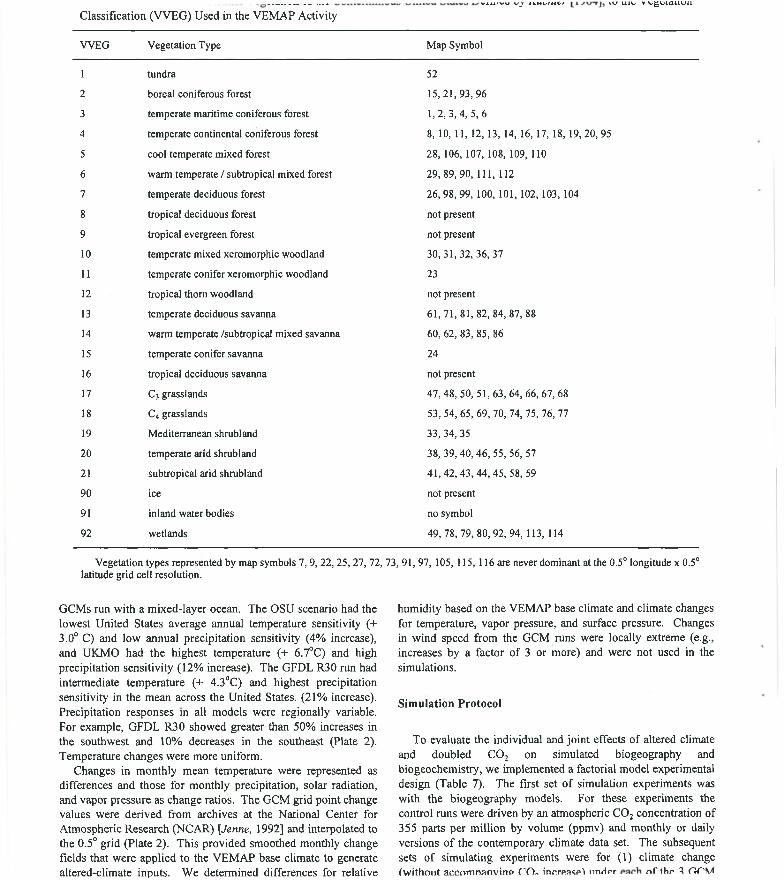
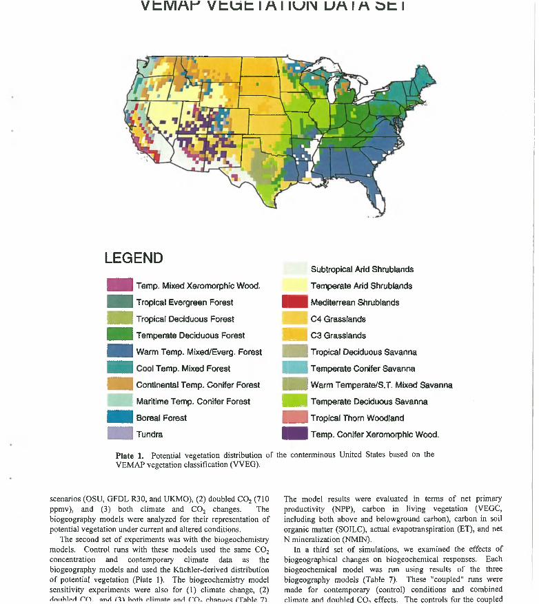
Our vegetation classification (VVEG) (Table 6 ) was developed by considering ( 1 ) the ability of the biogeography models to produce such a common classification, (2 ) the ability o f the biogeochemistry models to adapt their parameterizations to the classification, and (3) the vegetation classification used in extant georeferenced databases that describe the potential vegetation o f the conterminous United States. Vegetation classes were defined physiognomically in terms of dominant life-form and leaf characteristics (including leaf seasonal duration, shape, and size; Running et al. [1994]) and, in the case o f grasslands, physiologically with respect to dominance of species with the Cj versus C4 -photosynthetic pathway. Distribution of these types (Plate 1) was based on a gridded map of Kuchler's [1964, 1975] potential natural vegetation (D. W. Kicklighter and A. D. McGuire, personal communication, 1995). For the purpose o f this exercise, we assumed that this distribution o f potential vegetation is in equilibrium with current climate.

Required soil properties, including soil texture and depth (Table 4), were based on Kern's [1994,1995] 10-km gridded Soil Conservation Service national level (NATSGO) database. We used cluster analysis to group the 1 0 -km subgrid elements into 1 - 4 dominant ("modal") soil types for each 0.5° cell. In this approach we represented cell soil properties by one or more dominant soil profiles, rather than by an "average soil profile" that may not correspond to an actual soil in the region. Properties o f the first modal soil were used in the simulations. The models were applied to nonwetland areas (3168 total grid cells). Wetland or fioodplain ecosystems were excluded because some o f the models do not simulate water, carbon, or nitrogen dynamics for inundated soils.

C lim ate scenarios. Climate change scenarios used in the simulations were based on three atmospheric general circulation model (GCM) experiments for a doubled CO2 atmosphere and an equilibrium climate. These were from the Geophysical Fluid Dynamics Laboratory (GFDL) [R30 2.22° x 3.75° grid run; Manabe and Wetherald, 1990; and Wetherald and Manabe, 1990], Oregon State University (OSU) [Schlesinger and Zhao, 1989], and United Kingdom Meteorological Office (UKMO) [Wilson and Mitchell, 1987] (Plate 2). In these climate sensitivity experiments, the GCMs were implemented with a simple "mixed-layer" ocean representation that includes heat storage and vertical exchange o f heat and moisture with the atmosphere but omits horizontal ocean heat transport.

The three climate change scenarios were selected to represent the ranee o f climate sensitivity over the United States among

VOXAAAW^ \J J J k .M ^ /» » C / tV / U lC ' V W ^ L / i a U U i i

Classification (VVEG) Used in the VEMAP Activity

W E G Vegetation Type Map Symbol

1 tundra 52

2 boreal coniferous forest 1 5 ,2 1 ,9 3 ,9 6

3 temperate maritime coniferous forest 1 ,2 , 3 ,4 , 5 ,6

4 temperate continental coniferous forest 8 , 10, 11, 12, 13, 14, 16, 17, 18 ,19 , 20, 95

5 cool temperate mixed forest 28, 106, 107, 108, 109, 110

6 warm temperate / subtropical mixed forest 29, 89, 90, 111, 112

7 temperate deciduous forest 26, 9 8 ,9 9 , 100, 101, 102, 103,104

8 tropical deciduous forest not present

9 tropical evergreen forest not present

1 0 temperate mixed xeromorphic woodland 3 0 ,3 1 ,3 2 , 3 6 ,3 7

1 1 temperate conifer xeromorphic woodland 23

1 2 tropical thom woodland not present

13 temperate deciduous savanna 6 1 ,7 1 ,8 1 ,8 2 , 84, 87, 8 8

14 warm temperate /subtropical mixed savanna 60, 62, 83, 85, 8 6

15 temperate conifer savanna 24

16 tropical deciduous savanna not present

17 C3 grasslands 47, 48, 5 0 ,5 1 ,6 3 , 64, 6 6 , 67, 6 8

18 C4 grasslands 53, 54, 65, 69, 70, 74, 75, 76, 77

19 Mediterranean shrubland 33, 34, 35

2 0 temperate arid shrubland 38, 39, 40, 46, 55, 56, 57

2 1 subtropical arid shrubland 41, 42, 43, 44, 45, 58, 59

90 ice not present

91 inland water bodies no symbol

92 wetlands 49, 78, 79, 80, 92, 94 ,113 , 114

Vegetation types represented by map symbols 7, 9, 22, 25, 27, 72, 73, 91, 97, 105, 115, 116 are never dominant at the 0.5° longitude x 0.5° latitude grid cell resolution.

GCMs run with a mixed-layer ocean. The OSU scenario had the lowest United States average annual temperature sensitivity (+ 3.0° C) and low annual precipitation sensitivity (4% increase), and UKMO had the highest temperature (+ 6.7°C) and high precipitation sensitivity (12% increase). The GFDL R30 run had intermediate temperature (+ 4.3°C) and highest precipitation sensitivity in the mean across the United States. (21% increase). Precipitation responses in all models were regionally variable. For example, GFDL R30 showed greater than 50% increases in the southwest and 10% decreases in the southeast (Plate 2). Temperature changes were more uniform.

Changes in monthly mean temperature were represented as differences and those for monthly precipitation, solar radiation, and vapor pressure as change ratios. The GCM grid point change values were derived from archives at the National Center for Atmospheric Research (NCAR) [Jenne, 1992] and interpolated to the 0.5° grid (Plate 2). This provided smoothed monthly change fields that were applied to the VEM AP base climate to generate altered-climate inputs. We determined differences for relative

humidity based on the VEMAP base climate and climate changes for temperature, vapor pressure, and surface pressure. Changes in wind speed from the GCM runs were locally extreme (e.g., increases by a factor o f 3 or more) and were not used in the simulations.

Simulation Protocol

To evaluate the individual and joint effects of altered climate and doubled COj on simulated biogeography and biogeochemistry, we implemented a factorial model experimental design (Table 7). The first set o f simulation experiments was with the biogeography models. For these experiments the control runs were driven by an atmospheric COj concentration of 355 parts per million by volume (ppmv) and monthly or daily versions o f the contemporary climate data set. The subsequent sets o f simulating experiments were for ( 1 ) climate changetwithout accomnanvinp CO* inrrpficf^ nnrlfr rtf thf 3 OPM

V b M A r V t U t I A I l U I N U A I A C 3 t I

LEGEND

m i l Temp. Mixed Xeromorphic Wood,

m m Tropical Evergreen Forest |

i m H Tropical Deciduous Forest

m m Temperate Deciduous Forest 1

m m Warm Temp. Mixed/Everg. Forest |

m m Temp. Mixed Forest |

m m Continental Temp. Conifer Forest |

! Maritime Temp. Conifer Forest |

m m Boreal Forest |

m m i Tundra |

Plate 1. Potential vegetation distribution o f the VEMAP vegetation classification (VVEG).

Subtropical Arid Shrublands

Temperate Arid Shrublands

m i Mediterrean Shrublands

C4 Grasslands

1 ^ 1 C3 Grasslands

m i Tropical Deciduous Savanna

m i Temperate Conifer Savanna

m i Warm Temperate/S.T. Mixed Savanna

m i Temperate Deciduous Savanna

m i Tropical Thorn Woodland

m i Temp. Conifer Xeromorphic Wood.

conterminous United States based on the

scenarios (OSU, GFDL R30, and UKMO), (2) doubled COj (710 ppmv), and (3) both climate and COj changes. The biogeography models were analyzed for their representation of potential vegetation under current and altered conditions.

The second set o f experiments was with the biogeochemistry models. Control runs with these models used the same CO2

concentration and contemporary climate data as the biogeography models and used the Kiichler-derived distribution o f potential vegetation (Plate I). The biogeochemistry model sensitivity experiments were also for ( 1 ) climate change, (2 )/tnnh1p>H PO* iinH t't'i hntVi anrl PO - rhanofts fTahle 7V

The model results were evaluated in terms o f net primary productivity (NPP), carbon in living vegetation (VEGC, including both above and belowground carbon), carbon in soil organic matter (SOILC), actual evapotranspiration (ET), and net N mineralization (NMIN).

In a third set o f simulations, we examined the effects of biogeographical changes on biogeochemical responses. Each biogeochemical model was run using results o f the three biogeography models (Table 7). These "coupled" runs were made for contemporary (control) conditions and combined clim ate and doubled CO-, effects. The controls for the coupled

Annual T em perature C han ge D ifferenceOSU

9.00

7.25

5.90

■ 3.79

-L 2 .0 0

GFDL_R309.00

^■5.50

UKMO9.00

7.25

5.50

■ 3.75

L-L2 . 0 0

Annual Precipitation C h a n g e RatioOSU

•2.5

. 1.6

0.6

.0.4

GFDL-R30

UKMO

Plate 2. Changes in annual temperature and precipitation for doubled CO2 estimated by three atmospheric general circulation models, including: Oregon State University (OSU), the Geophysical Fluid Dynamics Laboratory (GFDL R30), and the United Kingdom M eteorological Office (UKMO); (a) Absolute change in mean annual surface air temperature, and (b) Ratio o f predicted to present precipitation.

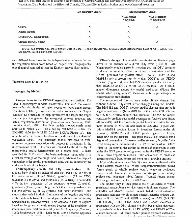
T a b le 7. Factorial D es ig n to E xam ine the In tluence o t C lim ate C hange and E levated A tm ospheric C D 2 C oncentration on Vegetation Distribution and the Effects o f Climate, CO 2 , and Biome Redistribution on Biogeochemical Processes

Biogeography Models Biogeochemistry Models

With KUchler Vegetation

With Vegetation Redistribution

Control X X X

Altered climate X X

Doubled CO2 concentration X X

Climate and CO2 change X X X

Control and doubled-C0 2 concentrations were 355 and 710 ppmv, respectively. Climate change scenarios were based on OSU, GFDL R30, and UKMO GCM experiments (see text).

runs differed from those for the independent experiments in that the vegetation fields were based on output from biogeography model control runs rather than the Ktichler-derived distribution.

Results and Discussion

B iogeography M odels

C om parisons to the V EM AP vegetation d is tribu tion . Thethree biogeography models successfully simulated the overall geographic distribution o f major vegetation types under current conditions (Plate 3). We used an index known as the “kappa statistic” as a measure o f map agreement: the larger the kappa statistic (k), the greater the agreement between modeled and actual vegetation distribution [Monserud and Leemans, 1992; Prentice et al., 1992]. The three models showed nearly equal abilities to match VVEG on a cell by cell basis {k = 0.69 for B I0M E2, 0.70 for MAPSS, 0.72 for DOLY; Figure la). The models had different misclassifications with respect to individual vegetation types. One consistent model bias was to over­represent montane vegetation with respect to shrublands in the intermountain west. This bias was caused by the difficulty o f representing spatial heterogeneity on a coarse grid. Climate specified for 0.5° cells in the basin-and-range topography is in effect an average o f the ranges and basins, whereas the mapped vegetation is the areally predominant type, that is, commonly the arid shrublands o f the basins.

C on tem porary clim ate and C O 2 concentration . The models have similar estimates o f area for forests (42 to 46% of the conterminous United States), grasslands (17 to 27%), savannas (15 to 25%), and shrublands (14 to 18%). The models differ in their placement o f the boundary between C 3 and C4

grasslands (Plate 3), reflecting the fact that these grasslands are not exclusively C 3 or C4 systems, but rather mixtures. The models also varied in their simulations o f the location and width o f the ecotone between the central grasslands and eastern forests, represented by savanna types. This ecotone is hard to capture based on long-term climatic means because of its sensitivity to interannual precipitation variability and fire frequency [Borchert, 1950; Daubenmire, 1968]. Each model uses a different approach

C lim ate change. The models' sensitivities to climate change differ in the absence o f a direct CO 2 effect (Plate 3). All biogeography models agree in showing that the OSU scenario produces the smallest effect on biome redistribution and the UKMO produces the greatest effect. Overall, B I0M E2 and MAPSS show a greater sensitivity than DOLY to the UKMO scenario (Figure la); and MAPSS shows a greater sensitivity than B I0M E 2 or DOLY to the GFDL scenario. As a result, greater divergence among the model predictions (Figure lb) occurs when using climate scenarios with larger changes in temperature or precipitation.

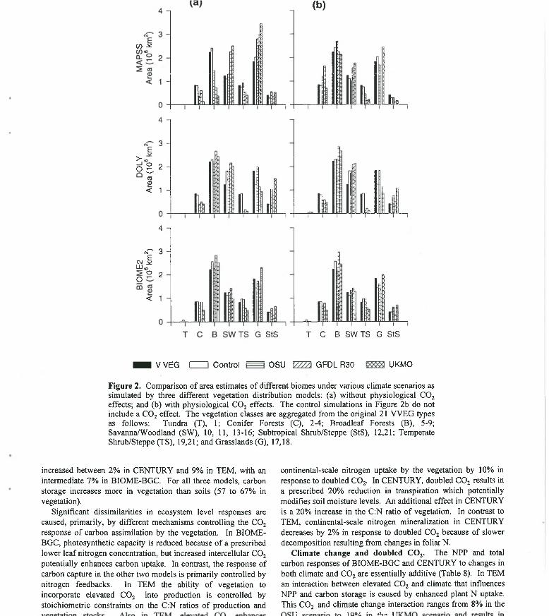
The responses o f forested area under climate change, but without a direct CO 2 effect, differ sharply among the models. The B I0M E2 and DOLY models predict changes that are both negative and positive (from -18% for DOLY under OSU climate to +7% for B I0M E 2 under GFDL climate). The MAPSS model consistently predicts substantial decreases in forested area (from -44 to -84%). All three models predict losses in conifer forests, most extreme in MAPSS and least in B10ME2 (Figure 2a). While MAPSS predicts losses in broadleaf forests under all scenarios, B I0M E 2 and DOLY predict gains or losses, depending on the scenario. The three models also predict some degree o f conversion o f westem conifer forests to broadleaf, the effect being most pronounced in B I0M E2 and least in DOLY (Plate 3). In general, the conifer to broadleaf conversion is least under the OSU scenario and greatest under the UKMO scenario for all three vegetation models. The conversion to broadleaf appears to result from longer and more moist growing seasons.

Most o f the simulations (Plate 3) show major northward shifts o f the eastem forest belts. Warm temperate/subtropical mixed forests partly or wholly replace today's temperate deciduous forests while temperate deciduous forests partly or wholly replace cool temperate mixed forests. Tropical forests extend their range northward in the B I0M E2 runs.

The models vary in their predictions o f the extent to which grasslands invade forests or vice versa with climate change. The BI0M E2 and MAPSS models predict that the areal extent o f grasslands increases for all climate change scenarios (Figure 2a); from +4% (B I0M E2 with GFDL climate) to +70% (MAPSS with UKMO). The DOLY model also predicts increases in grasslands with the OSU climate (+61%), but predicts decreases in grasslands with either the GFDL (-9%) and UKMO (-25%) climate scenarios. All three models predict eastward extensions

L.—

ail mree scenarios, especially in me upper u rea i LaKesregion o f the Midwest. The greatest change occurs with the MAPSS model under the UKMO climate where almost all o f the eastern forests are replaced by grasslands or savannas (Plate 3). In contrast, the DOLY model predicts only the eastward extension o f savannas into the Great Lakes region with climate change. In the southem plains, the models are in general agreement; they show expansions o f forests and savannas to the west under the high rainfall GFDL scenario and contractions o f these types to the east under both the OSU and UKMO scenarios. Within the central grasslands, the three models also predict some degree o f conversion o f C 3 grasslands to C4 grasslands because o f higher temperature and/or lower moisture availability; the effect being most pronounced in B I0M E2 under the UKMO climate and least pronounced in DOLY under the OSU climate.

All three biogeography models predict both positive and negative changes in the areal extent o f shmblands with climate change, but differ in the magnitude and direction o f these changes under a particular GCM climate (Figure 2a). Both the BI0M E2 and M APSS models predict an increase o f shmblands (+9.8 and +41.5%, respectively) under the OSU climate scenario, but predict a decrease o f shrublands in the warmer and wetter GFDL (-38.6% for B I0M E2; -6.2% for MAPSS) and UKMO (-8.5% for B I0M E 2; -0.6% for MAPSS) climate scenarios. Because grasses are better able to outcompete shmbs under more moist conditions, shrublands are replaced by grasslands in these latter GCM scenarios. In contrast, the DOLY model predicts a decrease in the areal extent o f shrublands for the OSU (-10.2%) and GFDL (-24.1%) scenarios, but predicts an increase of shrublands for the UKMO climate scenario (+29.5%). Within shrublands, all three models predict some degree o f conversion o f temperate arid shrublands to subtropical arid shmblands as a consequence o f the higher temperatures under the GCM scenarios; the effect is most pronounced in DOLY under the UKMO climate and least pronounced in MAPSS or BI0M E2 under the OSU climate.

Doubled C O j. All models show some direct effects o f COj on biome distribution in the absence o f climate change. The change is least for B I0M E 2 (Figure Ic, doubled CO2

comparisons), where the only major change is that C3 grasslands increase relative to C4 grasslands throughout the United States. The DOLY and MAPSS models show increases in the extent of forests through the westem interior and in the prairie-forest border region.

C lim ate change and doubled COj- A general result of considering both climate change and doubled CO 2 responses (Figures Ic -Id and Plate 4) is to substantially reduce the divergence among models by mitigating the climate-induced drought effects. The effect o f this CO 2 mitigation varies among the models. The B I0M E 2 model predicts changes o f forest area under climate change with doubled CO 2 that are similar to the changes o f forest area under climate change alone; forests increase under the GFDL climate (+10%), but decrease under the OSU (-14%) and UKMO (-14%) climates. In contrast, the MAPSS model predicts increases in forest area under the OSU (+23%) and GFDL (+20%) climates with doubled CO 2 as compared to the reductions o f forest area predicted under climate change alone. For the UKMO climate with doubled CO 2 , the MAPSS model predicts decreases in forest areas (-13%) that are

cnange aione. m e mixigaxion or ciimaxe-inaucea arougnx effects is also apparent in the DOLY model predictions of changes in forested area, but the effect is not as pronounced as the MAPSS model predictions; forested areas decrease under the OSU climate (-7%), but increase under the GFDL (+11%) and UKMO (+2%) climates. Within forests, the B I0M E2 and DOLY models still predict overall losses o f westem conifer forests under all three GCM scenarios while the MAPSS model predicts losses o f conifer forests only under the UKMO climate (Figure 2b). The MAPSS model predicts increases in conifer forests under both the OSU and GFDL climates.

As forested areas are generally predicted to increase under climate change with doubled CO 2 , the biogeography models predict either smaller increases or decreases in the areal extent of grasslands in comparison to climate change alone (Figure 2b). Both the B I0M E 2 and DOLY models predict that grasslands increase under the OSU climate (+10% for BI0M E2; +48% for DOLY) and decrease under the GFDL climate (-5% for B I0M E2; -8 % for DOLY), but the models differ in their response for the UKMO climate (+39% for BI0M E2; -31% for DOLY). Unlike the scenarios o f climate change alone, the MAPSS model predicts that grasslands will decrease for all climate scenarios with doubled CO 2 . The models still predict eastward extensions o f grasslands or savannas into the eastem broadleaf forests under all three GCM scenarios, but these extensions are more limited than predicted by the climate change alone scenarios; especially the changes predicted by the MAPSS model. The response o f grassland composition differs among the models. Climate change alone generally favors C4 grasses in all models. However, in B I0M E2 this effect is reversed by the CO2

fertilization o f C 3 grasses, which allows C3 grasslands to spread southward to Texas.

With climate change and elevated CO 2 , all biogeography models predict the areal extent o f shrublands to decrease for all GCM climates (from -75% for MAPSS under GFDL climate to -2% for DOLY under UKMO climate), with the exception o f B I0M E2 under the OSU climate which predicts increases in shmblands (+14%). Within shrublands, DOLY still predicts large increases in subtropical arid shmblands (+30 to +185%); B I0M E2 predicts gains or losses (-30 to +74%); and MAPSS predicts losses or small gains (-56 to +2%). With increased water use efficiency from elevated CO 2 , grasses are more able to gain a competitive advantage over shmbs to reduce the areal extent o f shmblands. Clearly for all biomes, the three biogeography models exhibit complex water balance responses, combining sensitivities to increases in temperature and rainfall with increased water use efficiency from elevated CO 2 .

B iogeochem istry Models

C on tem porary clim ate and C O 2 concentration. Thecontinental-scale estimates o f annual NPP for contemporary climate at an atmospheric concentration o f 355 ppmv CO 2 vary between 3125 x lO '^gC (TgC) y f ' and 3772 TgC y f ' (Table 8 ). This range is equivalent to the measurement error in NPP. The estimates for total carbon storage vary between 108 x lO'^ gC (PgC) and 118 PgC (Table 8 ), which represents a 9% difference among the models. Although the continental-scale estimates o f

u jrw A V .n n n

KHhbbN I ULIMA11 UhUL HaU ULIMAI h1 X C02 1 X C02

DOLY DOLY

BI0ME2BIOME2

MAPSSMAPSS

VEMAP VEGETATION DATA SET

W

Plate 3. The effect o f climate change on vegetation distribution. The simulated vegetation distributions o f the three biogeography models (DOLY, B I0M E2, and MAPSS) are compared to the VEM AP vegetation distribution and four climate scenarios: contemporary, OSU, GFDL R30, and UKMO. All simulations are based on an atmospheric COj concentration o f 355 ppmv.

UKMO CLIMATE 1 XC02

DOLY

OSU CLIMATE 1 X C02

DOLY

IBI0ME2BI0ME2

MAPSSMAPSS

LEGENDTemp. Mixed Xeromofphio Wood.

T r o i ^ Evergreen Forest

Tropicai Deciduous Forest

Temperate Deciduous Forest

Warm Temp. Mixed/Everg. Faest

Cool Temp. Mixed Forest

Continental Ten^. Coniier Forest

Maritime Temp. Conifer Forest

Boreai Forest

Tundra

Subtropical Arid Shnditands

Temperate Arid Shrublaniis

Medterrean Shmblands

C4 Grasslands

C3 Grasslands

Tropioal Deciduous Savanna

Temperate Ccmifer Savanna

Warm Temperate/S.T. Mixed Savanna

Temperate Dechfeous Savanna

Tropical Thom Woodland

Temp. Conifer Xeromorphic Wood.

V“ /

BIOME2 DOLY MAPSS BIOME2 BIOME2 DOLYVS v s vs

DOLY MAPSS MAPSS

(C)

0.6 -

0.4 - 0.2 -

0.0 -

BI0ME2 DOLY MAPSS

0.8 -

0.6 -

0.4 -

BI0ME2 BI0ME2 DOLY v s vs vs

DOLY MAPSS MAPSS

■ ■ V VEG I Control fgggi 2xC0

OSU V777A GFDLR30 UKMO

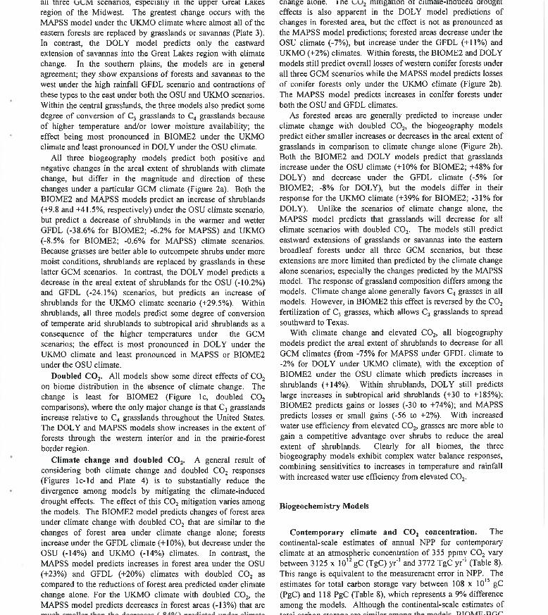
F igure 1. Comparison o f the kappa statistics among the VEMAP vegetation distribution (VVEG) and the simulated vegetation distributions o f the three biogeography models (BI0M E2, MAPSS, and DOLY) for various climate scenarios and atmospheric CO 2 scenarios: (a) the simulated vegetation distribution using current climate (Control) at an atmospheric CO 2 concentration o f 355 ppmv is compared to the VEMAP vegetation distribution and the simulated vegetation distributions o f the three biogeography models using the OSU, GFDL R30, and UKMO climates at an atmospheric CO2 concentration o f 355 ppmv; (b) the relative agreement between pairs o f biogeography models for various climate scenarios at an atmospheric CO 2

concentration o f 355 ppmv; (c) the simulated vegetation distribution using current climate (Control) at an atmospheric CO 2 concentration o f 355 ppmv is compared to the simulated vegetation distributions o f the three biogeography models using current, OSU, GFDL R30, and UKMO climates at an atmospheric CO 2 concentration o f 710 ppmv; and (d) the relative agreement between pairs o f biogeography models for various climate scenarios at an atmospheric CO2 concentration o f 710 ppmv. Large values o f the kappa statistic indicate good agreement between vegetation distributions.

estimates higher soil carbon (70 PgC) than the other two models (52 PgC by CENTURY and 49 PgC by TEM) and lower vegetation carbon (48 PgC) than either CENTURY (64 PgC) or TEM (59 PgC). The ecosystem level estimates o f NPP and total carbon storage are highly correlated (P < 0 .0 0 0 1 ; V = 17 ecosystems) among the models; in pairwise comparisons among the models the correlations range from 0.907 to 0.958 for NPP and from 0.954 to 0.970 for total carbon storage. The estimates for individual grid cells are also highly correlated (P < 0.0001; V = 3168 grid cells) among the models; correlations range from 0 .777 to 0 .k48 fnr NPP snH fl 8154 tn 0 01 1 fhr r'arhnn fltriraof*

IgW* A iiW WWAltAlAWAAtCtA IW V WA i'll A AWOpWAAOWO KJi.CENTURY and TEM to climate change are positive (Table 8 ) because both models estimate that nitrogen mineralization increases for the three climates (CENTURY, 10 to 19%, TEM, 8

to 11%). Enhanced nitrogen mineralization increases the amount o f nitrogen available to plants so that NPP may increase. For CENTURY, the response o f NPP and nitrogen mineralization is lowest for the low-temperature OSU scenario and highest for the high-temperature UKMO scenario. The CENTURY-estimated NPP o f warm temperate/subtropical mixed forest under the UKMO scenario increases 11%, and is associated with a 10% increase in nitrogen mineralization rates. Total carbon storage in CENTURY is enhanced by 4% for all climate scenarios (Table 8 ). Although CENTURY estimates losses o f soil C for all these climate scenarios, gains in vegetation C were 2 to 3 times as large as these losses.

In contrast to CENTURY, the NPP increases o f TEM (Table 8 ) are highest for the low-temperature OSU scenario (10%) and lowest for the high-temperature UKMO scenario (7%). The TEM estimates enhanced evaporative demand in warm temperate/subtropical mixed forest under the UKMO scenario, and predicts lower nitrogen cycling for UKMO than for OSU. Under the UKMO scenario, NPP for warm temperate/subtropical mixed forest decreases by 1 0 %, which is associated with a 1 2 % decrease in nitrogen mineralization. The response o f total carbon storage is correlated with the pattern o f NPP response and ranges from 1% increase for OSU to 11% decrease for UKMO (Table8 ). Thus although the NPP responses o f TEM and CENTURY both depend on the response o f nitrogen cycling to climate change, the models differ in how temperature and moisture availability influence nitrogen mineralization rates.

Among the three biogeochemistry models, BIOME-BGC generally estimates the most negative or smallest positive NPP responses to climate change (Table 8 ). The decrease in NPP for the UKMO scenario is primarily caused by lower production in warm temperate/subtropical mixed forest where mean annual air temperature increases 6.4°C and radiation increases 5.8%, but precipitation increases only 1.7%; the decrease in NPP is caused by increased evaporative demand. The model simulated increases in NPP for the GFDL scenario as a result o f reduced simulated evaporative demand for the GFDL scenario. The NPP response for the OSU scenario is intermediate because the low continental precipitation increase (4.3%) that is associated with low increases in temperature (+3.0°C) and solar radiation (1.6%) causes evaporative demand to increase slightly in the BIOME- BGC. The decreases in total carbon storage by BIOME-BGC range from 38% reduction for UKMO to 17% reduction for OSU (Table 8 ). For BIOME-BGC estimates o f total carbon storage to changes in climate are caused by decreases in NPP because of decreased water availabilities, and increases in plant and soil respiration because o f higher temperatures. Soil C loss accounts for 72 to 85% o f the total C loss across the three climate scenarios.

D oubled C O 2 .. Doubled atmospheric CO2 causes continental- scale increases in NPP that range from 5% in CENTURY to 11% in BIOME-BGC; TEM estimates an intermediate increase o f 9% (Table 8 ). These increases are substantially lower than the 25 to 50% growth response to doubled CO2 that has been observed in greenhouse studies that provide plants with sufficient nutrients anri lA/nfpr \J !rnhn}l 107^' 108^1 Tntal fa rhnn ctnram*

CO ^

I

^ (OO E

CO<D

3

2

< 1

4

cCT 3CM ^ LiJ<o

o 2o

< 1

(b)

hifl

T C B SW TS G StSStS

VVEG C Control OSU GFDL R30 UKMO

F igure 2. Comparison o f area estimates o f different biomes under various climate scenarios as simulated by three different vegetation distribution models: (a) without physiological COj effects; and (b) with physiological COj effects. The control simulations in Figure 2b do not include a CO 2 effect. The vegetation classes are aggregated from the original 21 VVEG types as follows: Tundra (T), 1; Conifer Forests (C), 2-4; Broadleaf Forests (B), 5-9;Savanna/W oodland (SW), 10, 11, 13-16; Subtropical Shrub/Steppe (StS), 12,21; Temperate Shrub/Steppe (TS), 19,21; and Grasslands (G), 17,18.

increased between 2% in CENTURY and 9% in TEM, with an intermediate 7% in BIOME-BGC. For all three models, carbon storage increases more in vegetation than soils (57 to 67% in vegetation).

Significant dissimilarities in ecosystem level responses are caused, primarily, by different mechanisms controlling the CO2

response o f carbon assimilation by the vegetation. In BIOME- BGC, photosynthetic capacity is reduced because o f a prescribed lower leaf nitrogen concentration, but increased intercellular CO2

potentially enhances carbon uptake. In contrast, the response of carbon capture in the other two models is primarily controlled by nitrogen feedbacks. In TEM the ability o f vegetation to incorporate elevated CO 2 into production is controlled by stoichiometric constraints on the C:N ratios o f production and

continental-scale nitrogen uptake by the vegetation by 1 0 % in response to doubled CO 2 . In CENTURY, doubled CO 2 results in a prescribed 2 0 % reduction in transpiration which potentially modifies soil moisture levels. An additional effect in CENTURY is a 20% increase in the C:N ratio o f vegetation. In contrast to TEM, continental-scale nitrogen mineralization in CENTURY decreases by 2 % in response to doubled CO 2 because o f slower decomposition resulting from changes in foliar N.

C lim ate change and doubled C O j. The NPP and total carbon responses o f BIOME-BGC and CENTURY to changes in both climate and CO 2 are essentially additive (Table 8 ). In TEM an interaction between elevated CO 2 and climate that influences NPP and carbon storage is caused by enhanced plant N uptake. This CO 2 and climate change interaction ranges from 8 % in the

T f y x 10 0 /1 f l i A T i t l

PRESENT CLIMATE QFDL R30 CLIMATE 1 X 002 2 X 002

DOLY DOLY

BI0ME2BIOME2

MAPSSMAPSS

VEMAP VEGETATION DATA SET

Plate 4. The effect o f climate change and doubled COj on vegetation distribution. The simulated vegetation distributions o f the three biogeography models (DOLY, BI0M E2, and MAPSS) are compared to the VEMAP vegetation distribution and four climate scenarios: contemporary, OSU, GFDL R30, and UKMO. The vegetation distribution for the contemporary climate is based on an atmospheric CO 2 concentration o f 355 ppmv. The vegetation distributions for the other climate scenarios are based on an atmospheric COj concentration o f 710 ppmv.

UKMU ULIMA I t2 X C 0 2

DOLY

U L IM A 1 12 X C 0 2

DOLY

BI0ME2BI0ME2

i

MAPSSMAPSS

LEGENDTsmp. Mixed XsromoipMc Wood

Trqpical Eveigreen Forest

Tropical Decidiioi» Forest

Temperate Deciduous Forest

Warm Temp. MixecVEverg. Forest

Cool Ten^. Mbred Forest

Gontinentai Temp. Conifsr Forest

MarHbneTemp. Conifer Forest

Boreal Forest

Tuncba

Temperate Arid Shrublands

Meditenean Shnit>iands

C4 Gmssiands

C3 Grasslands

Tropical Deciduous Savanna

Temperate Conilar Savanna

Warm Temperate/S.T. Mixed Savanna

Temperate Deciduous Savanna

Tropicai Thorn Woodland

Temp. Conifer Xeromorphic Wood.

Table 8. Continental-Scale Responses o f Net Primary Production and Total Carbon Storage (Vegetation plus Soils) to Doubled CO 2 , Climate Change, and Doubled CO 2 plus Climate Change as estimated by BIOME-BGC (BBGC), CENTURY (CEN), and the Terrestrial Ecosystem Model (TEM)

Annual Net Primary Production (lO'^ gC y f ’ or percent response)

Total Carbon Storage (lO'^ gC or percent response)

BBGC CEN TEM BBGC CEN TEM

Baseline estimates 3772 3125 3225 118 116 108

Response to climate change at IXCO 2

OSU -2.9% + 8 .8 % +10.3% -16.9% +3.5% +1.4%

GFDL +9.2% +15.5% +8.3% -18.4% +3.5% -4.6%

UKMO -6.5% +17.0% + 6 .6 % -37.6% +4.3% -10.9%

Response to 2 XCO2 + 1 0 .8 % +5.0% +8.7% +6.5% +2 .2 % +8.5%

Response to climate change at 2 XCO2

OSU +9.4% +14.6% +26.5% -9.1% +5.9% +16.1%

GFDL +2 0 .2 % +2 2 . 1 % +30.5% - 1 1 .0 % + 6 . 1 % +14.6%

UKMO +1.7% +23.6% +34.6% -32.7% +7.2% +12.3%

Interaction term between response to 2 XCO2 , climate, and 2 XCO2

plus climate

OSU +1.5% +0.9% +7.5% +1.4% + 0 . 1 % + 6 .2 %

GFDL + 0 .2 % + 1 .6 % +13.5% +0.9% +0.3% +10.7%

UKMO -2 .6 % +1.7% +19.4% - 1 .6 % + 0 .8 % +14.7%

V /V V 1 U .11 l l l W l WUOWkJ bAAUi.

similar effects for carbon storage (Table 8 ) Because of the interaction between elevated CO 2 and climate responses, TEM estimates the greatest enhancement in NPP and total carbon storage among the three biogeochemistry models.

Coupled Models

The coupled-model experiments involve spatially extrapolating the biogeochemistry models for the vegetation distributions that are defined by the biogeography models for each o f three GCM -generated climate scenarios. A coupling o f one biogeochemistry model with the vegetation of one biogeography model is hereafter referred to as a “model pair” . The biogeochemistry models did not determine the transient changes in NPP or carbon storage as vegetation changed on a grid cell. Instead, the biogeochemistry models simulated the equilibrium fluxes and pools for the new vegetation and climate o f the grid cell. For example, a grid cell that changed from a C3

grassland to a temperate deciduous forest used the parameters associated with temperate deciduous forests.

NPP and total carbon storage for contemporary climate. For contemporary climate at 355 ppmv COj, NPP for the three modeled vegetations varies among the biogeochemistry models from 3132 TgC yr'* (CENTURY with MAPSS vegetation) to 3854 TgC y f ' (BIOME-BGC with B I0M E2 vegetation) (Table9). The range is similar to that estimated among the three biogeochemistry models for the VEMAP vegetation distribution (Table 8 ). Thus the NPP estimates for a given biogeochemistry model are relatively constant among the different current vegetation distributions, with most o f the variability attributable to differences among the biogeochemistry models. Estimates for total carbon storage for the three current vegetation distributions range from 109 PgC (TEM with MAPSS vegetation) to 125 PgC (CENTURY with B I0M E 2 vegetation) (Table 9). Similar to NPP, most o f the variability is attributable to differences among the biogeochemistry models.

NPP responses to climate change and elevated carbon dioxide. The total continental-scale response o f NPP is calculated for each model pair by subtracting the NPP estimate for contemporary climate at 355 ppmv CO2 , from that for the future climate at doubled CO 2 ; and is relative to the estimate for contemporary climate (Table 9). The total NPP responses are positive for most o f the model pairs, but range widely. There are no relative increases in NPP when BIOME-BGC is run with either the DOLY or MAPSS vegetations for the UKMO climate (Table 9, Plate 5). The DOLY model simulates little change in the forested area o f the United States (42 to 43%), whereas MAPSS simulates a decrease from 44 to 38%. The largest NPP increases occur when the TEM is run with the MAPSS vegetation for the OSU climate (40%). The MAPSS model estimates that the forested area o f the conterminous United States increases from 44 to 53% under the OSU climate.

The total continental-scale NPP response for a model pair can be partitioned into two components (Table 10) (I) those resulting from changes in area o f ecosystems (i.e., structural responses), and (2) those resulting from a change in mean NPP for an ecosystem type based on the predictions o f the biogeochemistry tnnde»!s e . functional resnonsest. The structural resDonse for a

contemporary NPP (grams carbon per square meter per year) times the change in area estimated by the biogeography model. The continental-scale structural response for the model pair is determined by summing the structural response o f all vegetation types. The functional NPP response is determined by subtracting the structural response from the total response.

The structural response of NPP is generally positive because in most cases the biogeography models predict expansion o f high NPP ecosystems at the expense o f low NPP ecosystems. The functional NPP responses are specific to each biogeochemistry model: BIOM E-BGC’s range from -22% (DOLY for UKMO climate) to 7% (B I0M E2 for OSU climate), CENTURY’S are almost always positive with the largest being 14% (BI0M E2 for UKMO climate), and TEM ’s are always positive with the largest being 31% (B I0M E2 for OSU climate). The structural responses o f BIOME-BGC with all three biogeography model vegetations for the UKMO climate are effectively canceled by the functional NPP response o f BIOME-BGC to the UKMO climate. In contrast, the structural responses of NPP for the pairing o f TEM with all three biogeography model vegetations for the UKMO climate are enhanced by the functional responses o f TEM to this climate. There are two aspects to the mechanism underlying the functional NPP response o f TEM; increased nitrogen mineralization in response to elevated temperature, and increased nitrogen uptake. For model pairs involving either BIOME-BGC or CENTURY, the structural responses are generally equal to or greater than the functional responses (Table 10). In contrast, for model pairs involving TEM, the structural responses are generally less than the functional responses.

Carbon storage responses to climate change and elevated carbon dioxide. For the model pairs, both positive and negative changes o f total carbon storage occur (Table 9). Similar to NPP, the responses o f carbon storage range widely and depend on the combination o f climate scenario and model linkages. The largest carbon storage reduction, -39%, occurs when BIOME-BGC is run with the MAPSS vegetation for the UKMO climate (Table 9, Plate 6 ). This is an absolute loss of 47 PgC, o f which 33 Pg (70%) is from soil and 14 Pg (30%) is from vegetation. At the other extreme, the largest positive responses o f carbon storage, an increase o f 32%, occur when TEM is run with the MAPSS vegetations for the OSU and GFDL climates (Table 9). For the GFDL climate, this is an absolute increase of 35 PgC, o f which 5% is in soils and 95% is in vegetation.

The structural and functional responses for total carbon storage are calculated analogous to those for NPP. Both positive and negative structural responses occur (Table 10) and reflect changes in forest area predicted by the biogeography models. Similar to the NPP functional responses, those o f total carbon storage are specific to the different biogeochemistry models: BIOM E-BGC’s are always negative; CENTURY’S are always small and can be either positive or negative; and TEM ’s are always positive with the largest being 23%. The largest total carbon storage reduction, -39%, occurs when BIOME-BGC is run with the MAPSS vegetation for the UKMO climate. The decrease in forested area from 44 to 38% under this vegetation is responsible for the structural response. The functional response indicates a large reduction in carbon density within the forests. The reduction is caused by a combination of lower NPP due to water stress and higher plant respiration and decomposition

decomposition relationship is 2.4 as compared to approximately 2.0 in CENTURY and TEM; the for plant respiration are similar among the three models (2 .0 ).

The largest total carbon storage increase, 32%, occurs when TEM is run with the MAPSS vegetation for the OSU climate (Table 10) and is caused by an expansion o f forests from 44 to 53% o f the continental United States and temperature-enhanced nitrogen cycling. This forest expansion primarily replaces the shrublands.

Implications

The response o f ecosystems to changing climate is a central scientific issue for ( 1 ) understanding past states o f the Earth’s land surface and carbon cycle, (2 ) explaining the current state of ecosystems, and (3) predicting potential future responses to environmental change. While the first two issues are fundamental to ecological understanding and to establishing the credibility o f predictive models, the third one is important for policy makers considering the needs for greenhouse gas emission controls, and possible adaptation strategies. An objective of VEMAP was to provide preliminary information concerning the potential responses o f terrestrial ecosystems to climate change. The VEM AP exercise allowed us to identify common responses o f models and important differences. Where the models differ in their predictions, they reveal areas where our lack of understanding o f certain fundamental ecological processes limits our ability to narrow the range o f predictions, and points to areas o f research that could reduce uncertainties. The highly structured nature o f the intercomparison allowed rigorous intercomparison o f results, but also constrained the range o f questions explored. With VEM AP as a basis for understanding, future studies can explore a wider range o f questions, and implement more realistic conditions.

The VEM AP activity represents the state-of-the-art in terms of capabilities to project possible ecological effects o f climate change and elevated atmospheric CO 2 levels, and the projections can begin to provide policy makers with some sense o f the sensitivity o f natural ecosystems in the United States to these changes. The results clearly indicate that important properties of ecosystems, including the actual distribution o f major vegetation types, and such critical functional responses as primary productivity and carbon storage, could be highly sensitive to the magnitude o f climatic change that is predicted by some GCMs. However, there is considerable variation among models in the magnitude and even direction o f change.

Perhaps the most important messages that should be taken from the VEM AP exercise pertain to the identification of priorities for future research. We have identified the following four broad areas o f research as ones deserving immediate attention.

Modularization o f Models

We think that converting all o f the models to a modular structure will facilitate model comparisons and pairings. For a

w u

0^ 0^Tf

0^Tf 00 00

0’'in 0 in r-;

VO Os i—H 0 (N i—Hcn cn cn +

++

0^VO Ov VO Tf cn <N

cK rn rn (N 0 in in <Nrs (N <N

+ + + + + +

o’' 0^ 0^ 0’'<N cn 00 00 0 Os mcn 00 op 0 Os os <N

' '+

+ + +m+

(N (N (N

vO sO<N

0^00 <N

0 cn <N(N rs m m

+ + + + +

0’'(N m 0 <N

i—H 0 0 00 0 Os 00 Os(N rs rs (N <N m cn m+ + + + + + + + +

0^ 0^Os cn 0 VO p

vd in cn Os(N <N m cn

+ + + + + + +

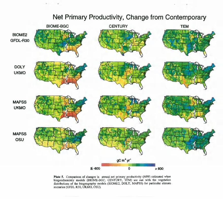
BI0ME2GFDL-R30

DOLYUKMO

MAPSSUKMO

MAPSSOSU

Net Primary Productivity, Change from ContemporaryBIOME-BGC CENTURY TEM

gC in'® yr

^ - 6 0 0 >600

Plate 5. Comparison o f changes in annual net primary productivity (NPP) estimated when biogeochemistry models (BIOME-BGC, CENTURY, TEM) are run with the vegetation distributions o f the biogeography models (BI0M E2, DOLY, MAPSS) for particular climate scenarios (GFDL R30, UKMO, OSU).

Table 10. The Total, Structural, and Functional Responses o f Annual Net Primary Production (NPP) and Total Carbon Storage for the Linkage o f the Three Biogeochemistry Models (BGC) (BIOME-BGC (BBGC), CENTURY (CEN), and the Terrestrial Ecosystem Model (TEM)) with the Vegetation Distributions o f the Three Biogeography Models (VEG) (BI0M E2, DOLY and MAPSS) for Contemporary Climate (CON) for the Three GCM Climates (OSU, GFDL, and UKMO) at 710 ppmv CO 2

Models Response Annual NPP (10*^ gC yr’’' or percent response) Total Carbon Storage (10*^ gC or percent response)

BGC VEG CON OSU GFDL UKMO CON OSU GFDL UKMO

BBGC BI0M E2 Total 3854 +7.4% +21.7% +0.4% 122 -13.2% -9.5% -34.7%Structural +0.2% +20.4% +7.1% -10.5% +7.9% -13.9%Functional +7.2% +1.3% -6.7% -2.7% -17.4% -20.8%

BBGC DOLY Total 3834 +5.6% +20.1% -0.1% 122 -18.1% -13.6% -36.4%Structural +11.3% +28.5% +21.8% -5.9% +5.0% -4.0%Functional -5.7% -8.4% -21.9% -12.2% -18.6% -32.4%

BBGC MAPSS Total 3798 +11.9% +20.4% -0.7% 120 -8.3% -13.9% -39.4%Structural +16.6% +17.6% +8.1% +8.6% +7.5% -12.6%Functional -4.7% +2.8% -8.8% -16.9% -21.4% -26.8%

CEN BI0M E2 Total 3200 +11.3% +18.4% +12.2% 125 -0.8% +12.6% -1.8%Structural -2.1% +14.5% -2.3% -5.1% +14.8% -2.3%Functional +13.4% +3.9% +14.5% +4.3% -2.2% +0.5%

CEN DOLY Total 3258 +26.0% +20.4% +14.7% 124 +9.8% +17.7% +7.8%Structural +12.5% +22.0% +15.1% +2.8% +17.7% +11.3%

Functional +13.5% -1.6% -0.4% +7.0% 0 .0% -3.5%

CEN MAPSS Total 3132 +15.6% +29.2% +20.3% 120 +17.0% +20.4% -1.5%Stractural +12.6% +22.7% +10.8% +16.5% +23.3% -2.1%

Functional +3.0% +6.5% +9.5% +0.5% -2.9% +0.6%

TEM BI0M E2 Total 3289 +27.0% +38.5% +27.8% 114 +11.9% +25.7% 0.0%Structural -3.8% +11.6% -0.4% -9.2% +11.7% -9.7%

Functional +30.8% +26.9% +28.2% +21.1% +14.0% +9.7%

TEM DOLY Total 3298 +33.1% +39.0% +33.2% 114 +19.7% +25.3% +12.5%Stractural +6.0% +17.6% +13.1% -3.0% +9.6% +1.4%Functional +27.1% +21.4% +20.1% +22.7% +15.7% +11.1%

TEM MAPSS Total 3288 +39.7% +37.2% +32.4% 109 +32.3% +32.2% +1.7%Stractural +10.9% +13.7% +8.7% +9.6% +14.9% -6.9%Functional +28.8% +23.5% +23.7% +22.7% +17.3% +8.6%

The reference for the responses are the estimates o f the biogeochemistry models for the vegetation distributions o f the biogeography models at contemporary climate (CON) and 355 ppmv CO2 .

BI0ME2GFDL-R30

DOLYUKMO

MAPSSUKMO

MAPSSOSU

Total Carbon Storage, Change from ContemporaryBIOME-BGC CENTURY

' T T T

g C m ‘

^36,OCX)

TEM

>36,000

Plate 6. Comparison o f changes in carbon stored in both vegetation and soils (total C) as estimated when biogeochemistry models (BIOME-BGC, CENTURY, TEM) are run with the vegetation distributions o f the biogeography models for particular climate scenarios (GFDL R30, UKMO, OSU).