Vector Spaces: Theory and Practice - University of Texas ... · PDF fileVector Spaces: Theory...
23
Chapter 5 Vector Spaces: Theory and Practice So far, we have worked with vectors of length n and performed basic operations on them like scaling and addition. Next, we looked at solving linear systems via Gaussian elimination and LU factorization. Already, we ran into the problem of what to do if a zero “pivot” is encountered. What if this cannot be fixed by swapping rows? Under what circumstances will a linear system not have a solution? When will it have more than one solution? How can we describe the set of all solutions? To answer these questions, we need to dive deeper into the theory of linear algebra. 5.1 Vector Spaces The reader should be quite comfortable with the simplest of vector spaces: R ,R 2 , and R 3 , which represent the points in one-dimentional, two-dimensional, and three-dimensional (real valued) space, respectively. A vector x ∈ R n is represented by the column of n real numbers x = χ 0 . . . χ n-1 which one can think of as the direction (vector) from the origin (the point 0= 0 . . . 0 ) to the point x = χ 0 . . . χ n-1 . However, notice that a direction is position independent: You can think of it as a direction anchored anywhere in R n . What makes the set of all vectors in R n a space is the fact that there is a scaling operation (multiplication by a scalar) defined on it, as well as the addition of two vectors: The definition of a space is a set of elements (in this case vectors in R n ) together with addition and multiplication (scaling) operations such that (1) for any two elements in the set, the element that results from adding these elements is also in the set; (2) scaling an element in the set results in an element in the set; and (3) there is an element in the set, denoted by 0, such that additing it to another element results in that element and scaling by 0 results in the 0 135
Transcript of Vector Spaces: Theory and Practice - University of Texas ... · PDF fileVector Spaces: Theory...

Chapter 5Vector Spaces: Theory and Practice
So far, we have worked with vectors of length n and performed basic operations on themlike scaling and addition. Next, we looked at solving linear systems via Gaussian eliminationand LU factorization. Already, we ran into the problem of what to do if a zero “pivot” isencountered. What if this cannot be fixed by swapping rows? Under what circumstanceswill a linear system not have a solution? When will it have more than one solution? Howcan we describe the set of all solutions? To answer these questions, we need to dive deeperinto the theory of linear algebra.
5.1 Vector Spaces
The reader should be quite comfortable with the simplest of vector spaces: R ,R2, and R3,which represent the points in one-dimentional, two-dimensional, and three-dimensional (realvalued) space, respectively. A vector x ! Rn is represented by the column of n real numbers
x =
!
"#!0...
!n!1
$
%& which one can think of as the direction (vector) from the origin (the point
0 =
!
"#0...0
$
%&) to the point x =
!
"#!0...
!n!1
$
%&. However, notice that a direction is position
independent: You can think of it as a direction anchored anywhere in Rn.What makes the set of all vectors in Rn a space is the fact that there is a scaling operation
(multiplication by a scalar) defined on it, as well as the addition of two vectors: The definitionof a space is a set of elements (in this case vectors in Rn) together with addition andmultiplication (scaling) operations such that (1) for any two elements in the set, the elementthat results from adding these elements is also in the set; (2) scaling an element in the setresults in an element in the set; and (3) there is an element in the set, denoted by 0, suchthat additing it to another element results in that element and scaling by 0 results in the 0
135
136 Chapter 5. Vector Spaces: Theory and Practice
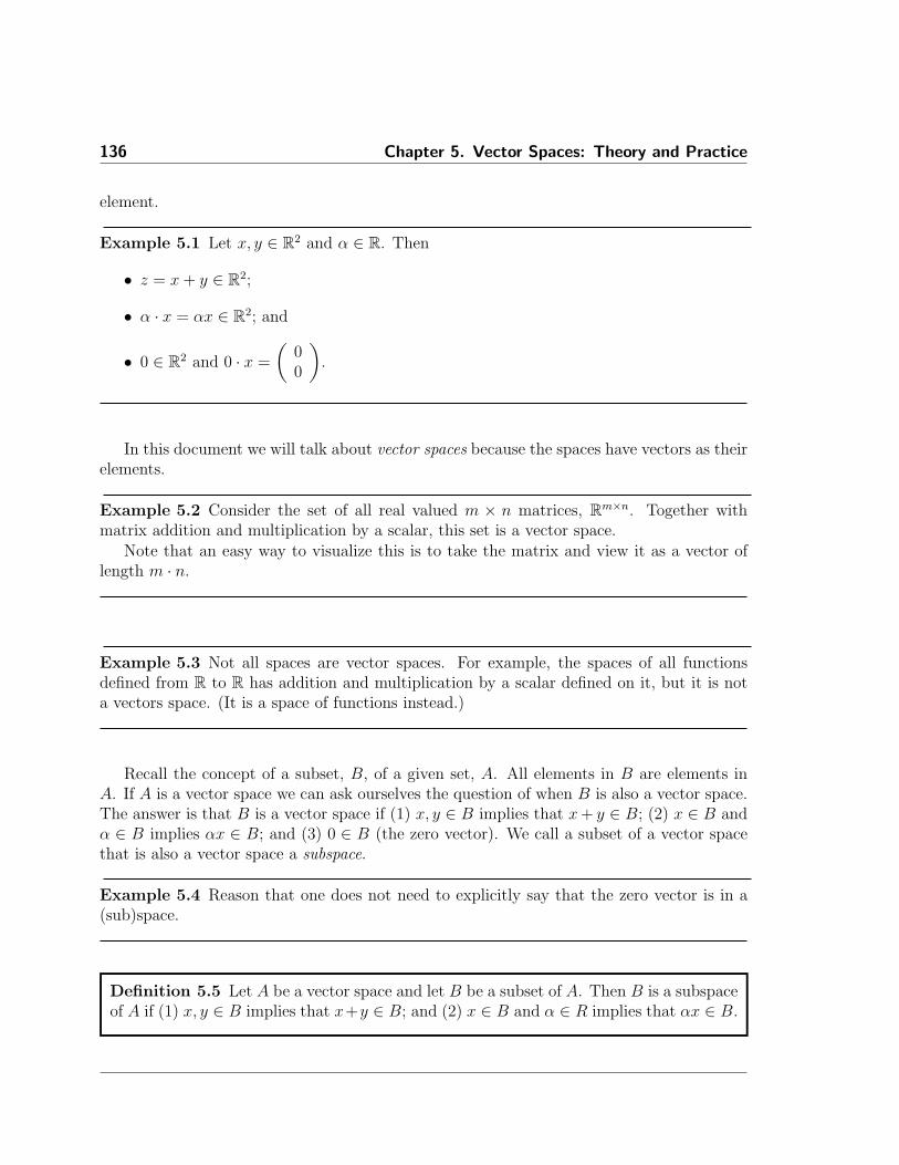
element.
Example 5.1 Let x, y ! R2 and " ! R. Then
• z = x + y ! R2;
• " · x = "x ! R2; and
• 0 ! R2 and 0 · x =
'00
(.
In this document we will talk about vector spaces because the spaces have vectors as theirelements.
Example 5.2 Consider the set of all real valued m " n matrices, Rm"n. Together withmatrix addition and multiplication by a scalar, this set is a vector space.
Note that an easy way to visualize this is to take the matrix and view it as a vector oflength m · n.
Example 5.3 Not all spaces are vector spaces. For example, the spaces of all functionsdefined from R to R has addition and multiplication by a scalar defined on it, but it is nota vectors space. (It is a space of functions instead.)
Recall the concept of a subset, B, of a given set, A. All elements in B are elements inA. If A is a vector space we can ask ourselves the question of when B is also a vector space.The answer is that B is a vector space if (1) x, y ! B implies that x + y ! B; (2) x ! B and" ! B implies "x ! B; and (3) 0 ! B (the zero vector). We call a subset of a vector spacethat is also a vector space a subspace.
Example 5.4 Reason that one does not need to explicitly say that the zero vector is in a(sub)space.
Definition 5.5 Let A be a vector space and let B be a subset of A. Then B is a subspaceof A if (1) x, y ! B implies that x+y ! B; and (2) x ! B and " ! R implies that "x ! B.
5.2. Why Should We Care? 137
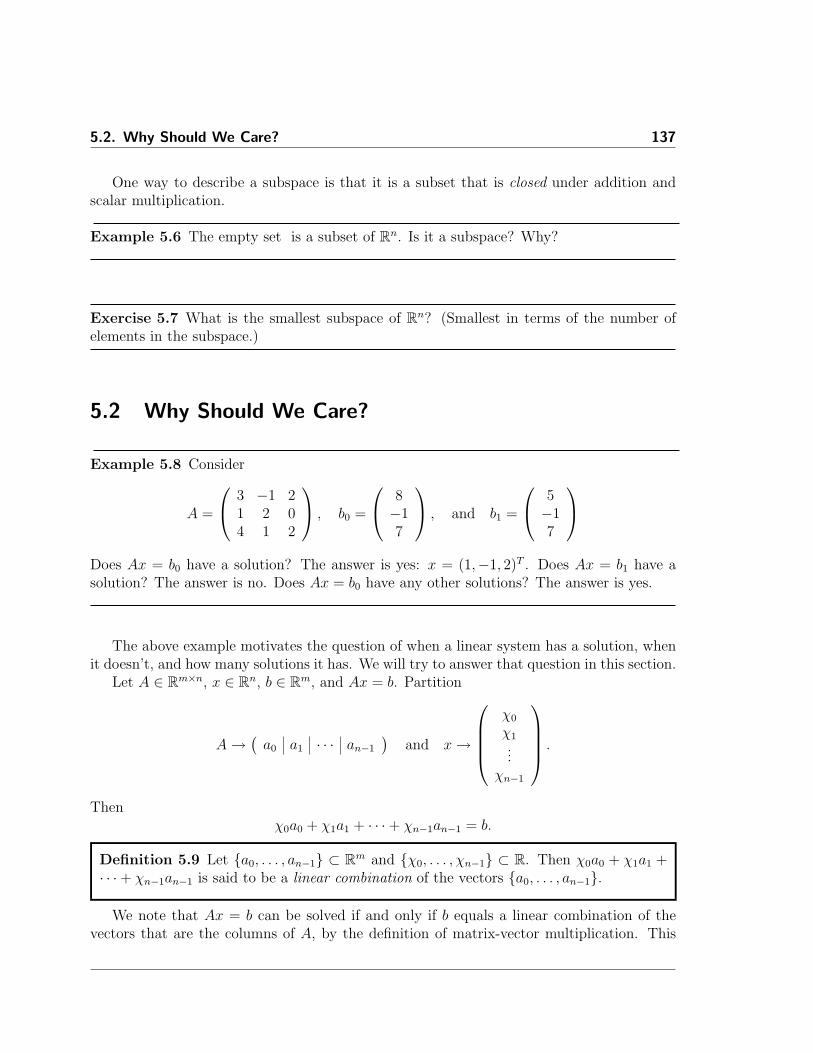
One way to describe a subspace is that it is a subset that is closed under addition andscalar multiplication.
Example 5.6 The empty set is a subset of Rn. Is it a subspace? Why?
Exercise 5.7 What is the smallest subspace of Rn? (Smallest in terms of the number ofelements in the subspace.)
5.2 Why Should We Care?
Example 5.8 Consider
A =
!
#3 #1 21 2 04 1 2
$
& , b0 =
!
#8#17
$
& , and b1 =
!
#5#17
$
&
Does Ax = b0 have a solution? The answer is yes: x = (1,#1, 2)T . Does Ax = b1 have asolution? The answer is no. Does Ax = b0 have any other solutions? The answer is yes.
The above example motivates the question of when a linear system has a solution, whenit doesn’t, and how many solutions it has. We will try to answer that question in this section.
Let A ! Rm"n, x ! Rn, b ! Rm, and Ax = b. Partition
A$)
a0 a1 · · · an!1
*and x$
!
"""#
!0
!1...
!n!1
$
%%%&.
Then!0a0 + !1a1 + · · · + !n!1an!1 = b.
Definition 5.9 Let {a0, . . . , an!1} % Rm and {!0, . . . ,!n!1} % R. Then !0a0 + !1a1 +· · · + !n!1an!1 is said to be a linear combination of the vectors {a0, . . . , an!1}.
We note that Ax = b can be solved if and only if b equals a linear combination of thevectors that are the columns of A, by the definition of matrix-vector multiplication. This

138 Chapter 5. Vector Spaces: Theory and Practice
observation answers the question “Given a matrix A, for what right-hand side vector, b, doesAx = b have a solution?” The answer is that there is a solution if and only if b is a linearcombination of the columns (column vectors) of A.
Definition 5.10 The column space of A ! Rm"n is the set of all vectors b ! Rm forwhich there exists a vector x ! Rn such that Ax = b.
Theorem 5.11 The column space of A ! Rm"n is a subspace (of Rm).
Proof: We need to show that the column space of A is closed under addition and scalarmultiplication:
• Let b0, b1 ! Rm be in the column space of A. Then there exist x0, x1 ! Rn such thatAx0 = b0 and Ax1 = b1. But then A(x0 + x1) = Ax0 + Ax1 = b0 + b1 and thus b0 + b1
is in the column space of A.
• Let b be in the column space of A and " ! R. Then there exists a vector x such thatAx = b and hence "Ax = "b. Since A("x) = "Ax = "b we conclude that "b is in thecolumn space of A.
Hence the column space of A is a subspace (of Rm).
Example 5.12 Consider again
A =
!
#3 #1 21 2 04 1 2
$
& , b0 =
!
#8#1
7
$
& .
Set this up as two appended systems, one for solving Ax = b0 and the other for solving Ax = 0(this will allow us to compare and contrast, which will lead to an interesting observation lateron): !
#3 #1 2 81 2 0 #14 1 2 7
$
&
!
#3 #1 2 01 2 0 04 1 2 0
$
& . (5.1)
Now, apply Gauss-Jordan elimination.
• It becomes convenient to swap the first and second equation:
!
#1 2 0 #13 #1 2 84 1 2 7
$
&
!
#1 2 0 03 #1 2 04 1 2 0
$
& .

5.2. Why Should We Care? 139
• Use the first row to eliminate the coe!cients in the first column below the diagonal:!
#1 2 0 #10 #7 2 110 #7 2 11
$
&
!
#1 2 0 00 #7 2 00 #7 2 0
$
& .
• Use the second row to eliminate the coe!cients in the second column below the diag-onal: !
#1 2 0 #10 #7 2 110 0 0 0
$
&
!
#1 2 0 00 #7 2 00 0 0 0
$
& .
• Divide the first and second row by the diagonal element:!
#1 2 0 #10 1 #2/7 #11/70 0 0 0
$
&
!
#1 2 0 00 1 #2/7 00 0 0 0
$
& .
• Use the second row to eliminate the coe!cients in the second column above the diag-onal: !
#1 0 4/7 15/70 1 #2/7 #11/70 0 0 0
$
&
!
#1 0 4/7 00 1 #2/7 00 0 0 0
$
& . (5.2)
Now, what does this mean? For now, we will focus only on the results for the appendedsystem
)A b0
*on the left.
• We notice that 0 " !2 = 0. So, there is no constraint on variable !2. As a result, wewill call !2 a free variable.
• We see from the second row that !1 # 2/7!2 = #11/7 or !1 = #11/7 + 2/7!2. Thus,the value of !1 is constrained by the value given to !2.
• Finally, !0 + 4/7!2 = 15/7 or !0 = 15/7 # 4/7!2. Thus, the value of !0 is alsoconstrained by the value given to !2.
We conclude that any vector of the form!
#15/7# 4/7!2
#11/7 + 2/7!2
!2
$
&
solves the linear system. We can rewrite this as!
#15/7#11/7
0
$
& + !2
!
##4/7
2/71
$
& . (5.3)
So, for each choice of !2, we get a solution to the linear system by plugging it into Equa-tion (5.3).

140 Chapter 5. Vector Spaces: Theory and Practice
Example 5.13 We now give a slightly “slicker” way to view Example 5.12. Consider againEquation (5.2): !
#1 0 4/7 15/70 1 #2/7 #11/70 0 0 0
$
& .
This represents !
#1 0 4/70 1 #2/70 0 0
$
&
!
#!0
!1
!2
$
& =
!
#15/7#11/7
0
$
& .
Using blocked matrix-vector multiplication, we find that'
!0
!1
(+ !2
'4/7#2/7
(=
'15/7#11/7
(
and hence '!0
!1
(=
'15/7#11/7
(# !2
'4/7#2/7
(
which we can then turn into!
#!0
!1
!2
$
& =
!
#15/7#11/7
0
$
& + !2
!
##4/7
2/71
$
&
In the above example, we notice the following:
• Let xp =
!
#15/7#11/7
0
$
&. Then Axp =
!
#3 #1 21 2 04 1 2
$
&
!
#15/7#11/7
0
$
& =
!
#8#1
7
$
&. In other
words, xp is a particular solution to Ax = b0. (Hence the p in the xp.)
• Let xn =
!
##4/7
2/71
$
&. Then Axn =
!
#3 #1 21 2 04 1 2
$
&
!
##4/7
2/71
$
& =
!
#000
$
&. We will see
that xn is in the null space of A, to be defined later. (Hence the n in xn.)
• Now, notice that for any ", xp + "xn is a solution to Ax = b0:
A(xp + "xn) = Axp + A("xn) = Axp + "Axn = b0 + "" 0 = b0.

5.2. Why Should We Care? 141
So, the system Ax = b0 has many solutions (indeed, an infinite number of solutions). Tocharacterize all solutions, it su!ces to find one (nonunique) particular solution xp thatsatisfies Axp = b0. Now, for any vector xn that has the property that Axn = 0, we knowthat xp + xn is also a solution.
Definition 5.14 Let A ! Rm"n. Then the set of all vectors x ! Rn that have theproperty that Ax = 0 is called the null space of A and is denoted by N (A).
Theorem 5.15 The null space of A ! Rm"n is a subspace of Rn.
Proof: Clearly N (A) is a subset of Rn. Now, assume that x, y ! N (A) and " ! R. ThenA(x + y) = Ax + Ay = 0 and therefore (x + y) ! N (A). Also A("x) = "Ax = " " 0 = 0and therefore "x ! N (A). Hence, N (A) is a subspace.
Notice that the zero vector (of appropriate length) is always in the null space of a matrixA.
Example 5.16 Let us use the last example, but with Ax = b1: Let us set this up as anappended system !
#3 #1 2 51 2 0 #14 1 2 7
$
& .
Now, apply Gauss-Jordan elimination.
• It becomes convenient to swap the first and second equation:!
#1 2 0 #13 #1 2 54 1 2 7
$
& .
• Use the first row to eliminate the coe!cients in the first column below the diagonal:!
#1 2 0 #10 #7 2 80 #7 2 11
$
& .
• Use the second row to eliminate the coe!cients in the second column below the diag-onal: !
#1 2 0 #10 #7 2 80 0 0 3
$
& .

142 Chapter 5. Vector Spaces: Theory and Practice
Now, what does this mean?
• We notice that 0 " !2 = 3. This is a contradiction, and therefore this linear systemhas no solution!
Consider where we started: Ax = b1 represents
3!0+ (#1)!1+ 2!2 = = 51!0+ 2!1+ (0)!2 = = #14!0+ !1+ 2!2 = = 7.
Now, the last equation is a linear combination of the first two. Indeed, add the first equationto the second, you get the third. Well, not quite: The last equation is actually inconsistent,because if you subtract the first two rows from the last, you don’t get 0 = 0. As a result,there is no way of simultaneously satisfying these equations.
5.2.1 A systematic procedure (first try)
Let us analyze what it is that we did in Examples 5.12 and 5.13.
• We start with A ! Rm"n, x ! Rn, and b ! Rm where Ax = b and x is to be computed.
• Append the system)
A b*.
• Use the Gauss-Jordan method to transform this appended system into the form
'Ik"k ATR bT
0(m!k)"k 0(m!k)"(n!k) bB
(, (5.4)
where Ik"k is the k " k identity matrix, ATR ! Rk"(n!k), bT ! Rk, and bB ! Rm!k.
• Now, if bB &= 0, then there is no solution to the system and we are done.
• Notice that (5.4) means that
'Ik"k ATR
0 0
( 'xT
xB
(=
'bT
0
(.
Thus, xT + ATRxB = bT . This translates to xT = bT # ATRxB or
'xT
xB
(=
'bT
0
(+
'#ATR
I(m!k)"(m!k)
(xB.

5.2. Why Should We Care? 143
• By taking xB = 0, we find a particular solution xp =
'bT
0
(.
• By taking, successively, xB = ei, i = 0, . . . , (m # k) # 1, we find vectors in the nullspace:
xni =
'#ATR
I(m!k)"(m!k)
(ei.
• The general solution is then given by
xp + "0xn0 + · · · + "(m!k)!1xn(m!k)!1.
Example 5.17 We now show how to use these insights to systematically solve the problemin Example 5.12. As in that example, create the appended systems for solving Ax = b0 andAx = 0 (Equation (5.1)).
!
#3 #1 2 81 2 0 #14 1 2 7
$
&
!
#3 #1 2 01 2 0 04 1 2 0
$
& . (5.5)
We notice that for Ax = 0 (the appended system on the right), the right-hand side neverchanges. It is always equal to zero. So, we don’t really need to carry out all the steps forit, because everything to the left of the | remains the same as it does for solving Ax = b.Carrying through with the Gauss-Jordan method, we end up with Equation (5.2):
!
#1 0 4/7 15/70 1 #2/7 #11/70 0 0 0
$
&
Now, our procedure tells us that xp =
!
#15/7#11/7
0
$
& is a particular solution: it solves Ax =
b. Next, we notice that
'ATR
I(m!k)"(m!k)
(=
!
#4/7#2/7
1
$
& so that ATR =
'4/7#2/7
(, and
I(m!k)"(m!k) = 1 (since there is only one free variable). So,
xn =
'#ATR
I(m!k)"(m!k)
(e0 =
!
##4/7
2/71
$
& 1 =
!
##4/7
2/71
$
&
The general solution is then given by
x = xp + "xn =
!
#15/7#11/7
0
$
& + "
!
##4/7
2/71
$
& ,
for any scalar ".

144 Chapter 5. Vector Spaces: Theory and Practice
5.2.2 A systematic procedure (second try)
Example 5.18 We now give an example where the procedure breaks down. Note: thisexample is borrowed from the book.
Consider Ax = b where
A =
!
#1 3 3 22 6 9 7#1 #3 3 4
$
& and b =
!
#2
1010
$
& .
Let us apply Gauss-Jordan to this:
• Append the system: !
#1 3 3 2 22 6 9 7 10#1 #3 3 4 10
$
& .
• The boldfaced “1” is the pivot, in the first column. Subtract 2/1 times the first rowand (#1)/1 times the first row from the second and third row, respectively:
!
#1 3 3 2 20 0 3 3 60 0 6 6 12
$
& .
• The problem is that there is now a “0” in the second column. So, we skip it, and moveon to the next column. The boldfaced “3” now becomes the pivot. Subtract 6/3 timesthe second row from the third row:
!
#1 3 3 2 20 0 3 3 60 0 0 0 0
$
& .
• Divide each (nonzero) row by the pivot in that row to obtain
!
#1 3 3 2 20 0 1 1 20 0 0 0 0
$
& .

5.2. Why Should We Care? 145
• We can only eliminate elements in the matrix above pivots. So, take 3/1 times thesecond row and subtract from the first row:
!
#1 3 0 #1 #40 0 1 1 20 0 0 0 0
$
& . (5.6)
• This does not have the form advocated in Equation 5.4. So, we remind ourselves ofthe fact that Equation 5.6 stands for
!
#1 3 0 #10 0 1 10 0 0 0
$
&
!
""#
!0
!1
!2
!3
$
%%& =
!
##4
20
$
& (5.7)
Notice that we can swap the second and third column of the matrix as long as we alsoswap the second and third element of the solution vector:
!
#1 0 3 #10 1 0 1
0 0 0 0
$
&
!
""#
!0
!2
!1
!3
$
%%& =
!
##4
20
$
& . (5.8)
• Now, we notice that !1 and !3 are the free variables, and with those we can findequations for !0 and !2 as before.
• Also, we can now find vectors in the null space just as before. We just have to payattention to the order of the unknowns (the order of the elements in the vector x).
In other words, a specific solution is now given by
xp
!
""#
!0
!2
!1
!3
$
%%& =
!
""#
#4200
$
%%&
and two linearly independent vectors in the null space are given by the columns of!
""#
#3 10 #11 00 1
$
%%&
giving us a general solution of!
""#
!0
!2
!1
!3
$
%%& =
!
""#
#4200
$
%%& + "
!
""#
3010
$
%%& + #
!
""#
1#1
01
$
%%& .
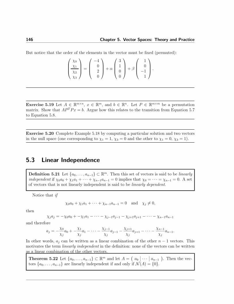
146 Chapter 5. Vector Spaces: Theory and Practice
But notice that the order of the elements in the vector must be fixed (permuted):!
""#
!0
!1
!2
!3
$
%%& =
!
""#
#4020
$
%%& + "
!
""#
3100
$
%%& + #
!
""#
10#1
1
$
%%& .
Exercise 5.19 Let A ! Rm"n, x ! Rm, and b ! Rn. Let P ! Rm"m be a permutationmatrix. Show that AP T Px = b. Argue how this relates to the transition from Equation 5.7to Equation 5.8.
Exercise 5.20 Complete Example 5.18 by computing a particular solution and two vectorsin the null space (one corresponding to !1 = 1, !3 = 0 and the other to !1 = 0, !3 = 1).
5.3 Linear Independence
Definition 5.21 Let {a0, . . . , an!1} % Rm. Then this set of vectors is said to be linearlyindependent if !0a0 + !1a1 + · · · + !n!1an!1 = 0 implies that !0 = · · · = !n!1 = 0. A setof vectors that is not linearly independent is said to be linearly dependent.
Notice that if
!0a0 + !1a1 + · · · + !n!1an!1 = 0 and !j &= 0,
then!jaj = #!0a0 +#!1a1 # · · ·# !j!1aj!1 # !j+1aj+1 # · · ·# !n!1an!1
and therefore
aj = #!0
!ja0 +#!1
!ja1 # · · ·# !j!1
!jaj!1 #
!j+1
!jaj+1 # · · ·# !n!1
!jan!1.
In other words, aj can be written as a linear combination of the other n # 1 vectors. Thismotivates the term linearly independent in the definition: none of the vectors can be writtenas a linear combination of the other vectors.
Theorem 5.22 Let {a0, . . . , an!1} % Rm and let A =)
a0 · · · an!1
*. Then the vec-
tors {a0, . . . , an!1} are linearly independent if and only if N (A) = {0}.

5.3. Linear Independence 147
Proof:
(') Assume {a0, . . . , an!1} are linearly independent. We need to show that N (A) = {0}.
Assume x ! N (A). Then Ax = 0 implies that 0 = Ax =)
a0 · · · an!1
*!
"#!0...
!n!1
$
%& =
!0a0 + !1a1 + · · · + !n!1an!1 and hence !0 = · · · = !n!1 = 0. Hence x = 0.
(() Notice that we are trying to prove P ) Q, where P represents “the vectors {a0, . . . , an!1}are linearly independent” and Q represents “N (A) = {0}”. It su!ces to prove the con-verse: ¬P $ ¬Q. Assume that {a0, . . . , an!1} are not linearly independent. Then thereexist {!0, · · · , !n!1} with at least one !j &= 0 such that !0a0+!1a1+· · ·+!n!1an!1 = 0.Let x = (!0, . . . ,!n!1)T . Then Ax = 0 which means x ! N (A) and hence N (A) &= {0}.
Example 5.23 The columns of an identity matrix I ! Rn"n form a linearly independentset of vectors.
Proof: Since I has an inverse (I itself) we know that N (I) = {0}. Thus, by Theorem 5.22,the columns of I are linearly independent.
Example 5.24 The columns of L =
!
#1 0 02 #1 01 2 3
$
& are linearly independent. If we consider
!
#1 0 02 #1 01 2 3
$
&
!
#!0
!1
!2
$
& =
!
#000
$
&
and simply solve this, we find that !0 = 0/1 = 0, !1 = (0# 2!0)/(#1) = 0, and !2 = (0#!0#2!1)/(3) = 0. Hence, N (L) = {0} (the zero vector) and we conclude, by Theorem 5.22,that the columns of L are linearly independent.
The last example motivates the following theorem:

148 Chapter 5. Vector Spaces: Theory and Practice
Theorem 5.25 Let L ! Rn"n be a lower triangular matrix with nonzeroes on its diago-nal. Then its columns are linearly independent.
Proof: Let L be as indicated and consider Lx = 0. If one solves this via whatever methodone pleases, the solution x = 0 will emerge as the only solution. Thus N (L) = {0} and byTheorem 5.22, the columns of L are linearly independent.
Exercise 5.26 Let U ! Rn"n be an upper triangular matrix with nonzeroes on its diagonal.Then its columns are linearly independent.
Exercise 5.27 Let L ! Rn"n be a lower triangular matrix with nonzeroes on its diagonal.Then its rows are linearly independent. (Hint: How do the rows of L relate to the columnsof LT ?)
Example 5.28 The columns of L =
!
""#
1 0 02 #1 01 2 3#1 0 #2
$
%%& are linearly independent. If we
consider !
""#
1 0 02 #1 01 2 3#1 0 #2
$
%%&
!
#!0
!1
!2
$
& =
!
""#
0000
$
%%&
and simply solve this, we find that !0 = 0/1 = 0, !1 = (0# 2!0)/(#1) = 0, !2 = (0# !0 #2!1)/(3) = 0. Hence, N (L) = {0} (the zero vector) and we conclude, by Theorem 5.22, thatthe columns of L are linearly independent.
This example motivates the following general observation:
Theorem 5.29 Let A ! Rm"n have linearly independent columns and let B ! Rk"n.
Then the matrices
'AB
(and
'BA
(have linearly independent columns.
5.4. Bases 149
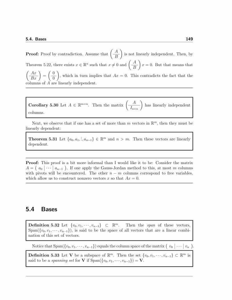
Proof: Proof by contradiction. Assume that
'AB
(is not linearly independent. Then, by
Theorem 5.22, there exists x ! Rn such that x &= 0 and
'AB
(x = 0. But that means that
'AxBx
(=
'00
(, which in turn implies that Ax = 0. This contradicts the fact that the
columns of A are linearly independent.
Corollary 5.30 Let A ! Rm"n. Then the matrix
'A
In"n
(has linearly independent
columns.
Next, we observe that if one has a set of more than m vectors in Rm, then they must belinearly dependent:
Theorem 5.31 Let {a0, a1,..., an!1} ! Rm and n > m. Then these vectors are linearly
dependent.
Proof: This proof is a bit more informal than I would like it to be: Consider the matrixA =
)a0 · · · an!1
*. If one apply the Gauss-Jordan method to this, at most m columns
with pivots will be encountered. The other n # m columns correspond to free variables,which allow us to construct nonzero vectors x so that Ax = 0.
5.4 Bases
Definition 5.32 Let {v0, v1, · · · , vn!1} % Rm. Then the span of these vectors,Span({v0, v1, · · · , vn!1}), is said to be the space of all vectors that are a linear combi-nation of this set of vectors.
Notice that Span({v0, v1, · · · , vn!1}) equals the column space of the matrix)
v0 · · · vn
*.
Definition 5.33 Let V be a subspace of Rm. Then the set {v0, v1, · · · , vn!1} % Rm issaid to be a spanning set for V if Span({v0, v1, · · · , vn!1}) = V.

150 Chapter 5. Vector Spaces: Theory and Practice
Definition 5.34 Let V be a subspace of Rm. Then the set {v0, v1, · · · , vn!1} % Rm
is said to be a basis for V if (1) {v0, v1, · · · , vn!1} are linearly independent and (2)Span({v0, v1, · · · , vn!1}) = V.
The first condition says that there aren’t more vectors than necessary in the set. Thesecond says there are enough to be able to generate V.
Example 5.35 The vectors {e0, . . . , em!1} % Rm, where ej equals the jth column of theidentity, are a basis for Rm.
Note: these vectors are linearly independent and any vector x ! Rm with x =
!
"#!0...
!m!1
$
%&
can be written as the linear combination !0e0 + · · · + !m!1em!1.
Example 5.36 Let {a0, . . . , am!1} % Rm and let A =)
a0 · · · am!1
*be invertible. Then
{a0, . . . , am!1} % Rm form a basis for Rm.Note: The fact that A is invertible means there exists A!1 such that A!1A = I. Since
Ax = 0 means x = A!1Ax = A!10 = 0, the columns of A are linearly independent. Also,given any vector y ! Rm, there exists a vector x ! Rm such that Ax = y (namely x = A!1y).
Letting x =
!
"#!0...
!m!1
$
%& we find that y = !0a0 + · · · + !m!1am!1 and hence every vector in
Rm is a linear combination of the set {a0, . . . , am!1} % Rm.
Now here comes a very important insight:
Theorem 5.37 Let V be a subspace of Rm and let {v0, v1, · · · , vn!1} % Rm and{w0, w1, · · · , wk!1} % Rm both be bases for V. Then k = n. In other words, the numberof vectors in a basis is unique.
Proof: Proof by contradiction. Without loss of generality, let us assume that k > n.(Otherwise, we can switch the roles of the two sets.) Let V =
)v0 · · · vn!1
*and W =)
w0 · · · wk!1
*. Let xj have the property that wj = V xj. (We know such a vector xj
exists because V spans V and wj ! V.) Then W = V X, where X =)
x0 · · · xk!1
*.
Now, X ! Rn"k and recall that k > n. This means that N (X) contains nonzero vectors(why?). Let y ! N (X). Then Wy = V Xy = V (Xy) = V (0) = 0, which contradicts the fact

5.5. Exercises 151
that {w0, w1, · · · , wk!1} are linearly independent, and hence this set cannot be a basis for V.
Note: generally speaking, there are an infinite number of bases for a given subspace.(The exception is the subspace {0}.) However, the number of vectors in each of these basesis always the same. This allows us to make the following definition:
Definition 5.38 The dimension of a subspace V equals the number of vectors in a basisfor that subspace.
A basis for a subspace V can be derived from a spanning set of a subspace V by, one-to-one, removing vectors from the set that are dependent on other remaining vectors untilthe remaining set of vectors is linearly independent , as a consequence of the followingobservation:
Definition 5.39 Let A ! Rm"n. The rank of A equals the number of vectors in a basisfor the column space of A. We will let rank(A) denote that rank.
Theorem 5.40 Let {v0, v1, · · · , vn!1} % Rm be a spanning set for subspace Vand assume that vi equals a linear combination of the other vectors. Then{v0, v1, · · · , vi!1, vi, vi!1, · · · , vn!1} is a spanning set of V.
Similarly, a set of linearly independent vectors that are in a subspace V can be “builtup” to be a basis by successively adding vectors that are in V to the set while maintainingthat the vectors in the set remain linearly independent until the resulting is a basis for V.
Theorem 5.41 Let {v0, v1, · · · , vn!1} % Rm be linearly independent and assume that{v0, v1, · · · , vn!1} % V . Then this set of vectors is either a spanning set for V or thereexists w ! V such that {v0, v1, · · · , vn!1, w} are linearly independent.
5.5 Exercises
(Most of these exercises are borrowed from “Linear Algebra and Its Application” by GilbertStrang.)
1. Which of the following subsets of R3 are actually subspaces?
(a) The plane of vectors x = (!0, !1, !2)T ! R3 such that the first component !0 = 0.In other words, the set of all vectors
!
#0!1
!2
$
&

152 Chapter 5. Vector Spaces: Theory and Practice
where !1, !2 ! R.
(b) The plane of vectors x with !0 = 1.
(c) The vectors x with !1!2 = 0 (this is a union of two subspaces: those vectors with!1 = 0 and those vectors with !2 = 0).
(d) All combinations of two given vectors (1, 1, 0)T and (2, 0, 1)T .
(e) The plane of vectors x = (!0, !1, !2)T that satisfy !2 # !1 + 3!0 = 0.
2. Describe the column space and nullspace of the matrices
A =
'1 #10 0
(, B =
'0 0 31 2 3
(, and C =
'0 0 00 0 0
(.
3. Let P % R3 be the plane with equation x + 2y + z = 6. What is the equation of theplane P0 through the origin parallel to P? Are P and/or P0 subspaces of R3?
4. Let P % R3 be the plane with equation x + y # 2z = 4. Why is this not a subspace?Find two vectors, x and y, that are in P but with the property that x + y is not.
5. Find the echolon form U , the free variables, and the special (particular) solution ofAx = b for
(a) A =
'0 1 0 30 2 0 6
(, b =
'#0
#1
(. When does Ax = b have a solution? (When
#1 = ?.) Give the complete solution.
(b) A =
!
""#
0 01 20 03 6
$
%%&, b =
!
""#
#0
#1
#2
#3
$
%%&. When does Ax = b have a solution? (When ...)
Give the complete solution.
6. Write the complete soluton x = xp + xn to these systems:
'1 2 22 4 5
( !
#uvw
$
& =
'14
(
and'
1 2 22 4 4
( !
#uvw
$
& =
'14
(
7. Which of these statements is a correct definition of the rank of a given matrix A !Rm"n? (Indicate all correct ones.)
5.5. Exercises 153
(a) The number of nonzero rows in the row reduced form of A.
(b) The number of columns minus the number of rows, n#m.
(c) The number of columns minus the number of free columns in the row reducedform of A. (Note: a free column is a column that does not contain a pivot.)
(d) The number of 1s in the row reduced form of A.
8. Let A, B ! Rm"n, u ! Rm, and v ! Rn. The operation B := A + "uvT is often calleda rank-1 update. Why?
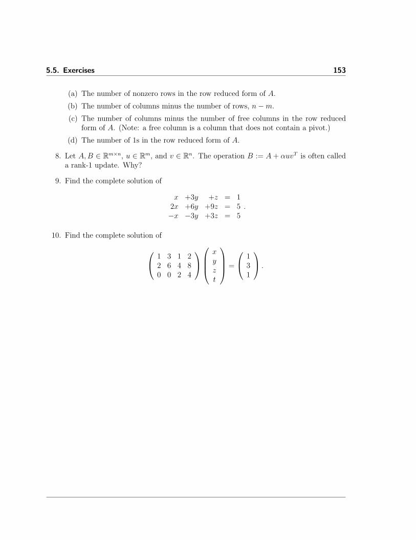
9. Find the complete solution of
x +3y +z = 12x +6y +9z = 5#x #3y +3z = 5
.
10. Find the complete solution of
!
#1 3 1 22 6 4 80 0 2 4
$
&
!
""#
xyzt
$
%%& =
!
#131
$
& .
154 Chapter 5. Vector Spaces: Theory and Practice
5.6 The Answer to Life, The Universe, and Everything
We complete this chapter by showing how many answers about subspaces can be answeredfrom the upper-echolon form of the linear system.
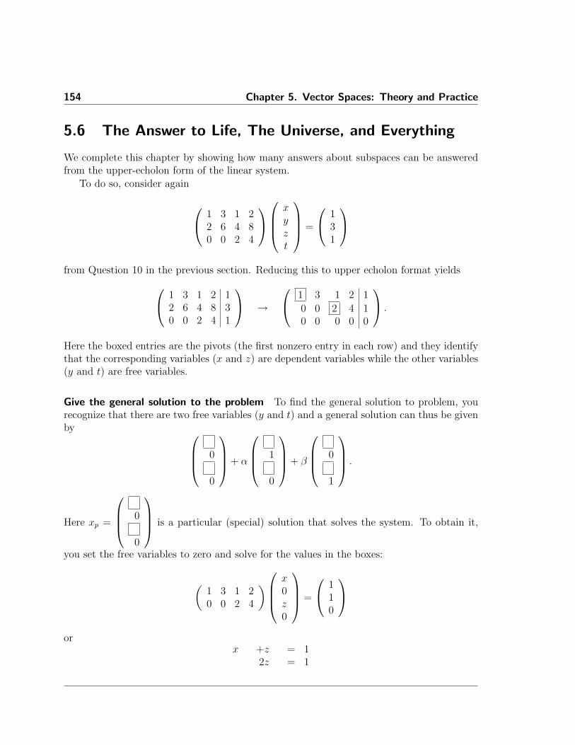
To do so, consider again
!
#1 3 1 22 6 4 80 0 2 4
$
&
!
""#
xyzt
$
%%& =
!
#131
$
&
from Question 10 in the previous section. Reducing this to upper echolon format yields
!
#1 3 1 2 12 6 4 8 30 0 2 4 1
$
& $
!
#1 3 1 2 10 0 2 4 10 0 0 0 0
$
& .
Here the boxed entries are the pivots (the first nonzero entry in each row) and they identifythat the corresponding variables (x and z) are dependent variables while the other variables(y and t) are free variables.
Give the general solution to the problem To find the general solution to problem, yourecognize that there are two free variables (y and t) and a general solution can thus be givenby !
""#0
0
$
%%& + "
!
""#1
0
$
%%& + #
!
""#0
1
$
%%& .
Here xp =
!
""#0
0
$
%%& is a particular (special) solution that solves the system. To obtain it,
you set the free variables to zero and solve for the values in the boxes:
'1 3 1 20 0 2 4
(!
""#
x0z0
$
%%& =
!
#110
$
&
orx +z = 1
2z = 1

5.6. The Answer to Life, The Universe, and Everything 155
so that z = 1/2 and x = 1/2 yielding a particular solution xp =
!
""#
1/20
1/20
$
%%&.
Next, we have to find the two vectors in the null space of the matrix. To obtain the first,we set the first free variable to one and the other(s) to zero:
'1 3 1 20 0 2 4
(!
""#
x1z0
$
%%& =
!
#000
$
&
orx +3" 1 +z = 0
2z = 0
so that z = 0 and x = #3, yielding the first vector in the null space xn0 =
!
""#
#3100
$
%%&.
To obtain the second, we set the second free variable to one and the other(s) to zero:
'1 3 1 20 0 2 4
(!
""#
x0z1
$
%%& =
!
#000
$
&
orx +z +2" 1 = 0
2z +4" 1 = 0
so that z = #4/2 = #2 and x = #z # 2 = 0, yielding the second vector in the null space
xn1 =
!
""#
00#2
1
$
%%&.
And thus the general solution is given by!
""#
1/20
1/20
$
%%& + "
!
""#
#3100
$
%%& + #
!
""#
00#2
1
$
%%& ,
where " and # are scalars.
Find a specific (particular) solution to the problem The above procedure yields theparticular solution as part of the first step.
156 Chapter 5. Vector Spaces: Theory and Practice
Find vectors in the null space The first step is to figure out how many (linear independent)vectors there are in the null space. This equals the number of free variables. The aboveprocedure then gives you a step-by-step procedure for finding that many linearly independentvectors in the null space.
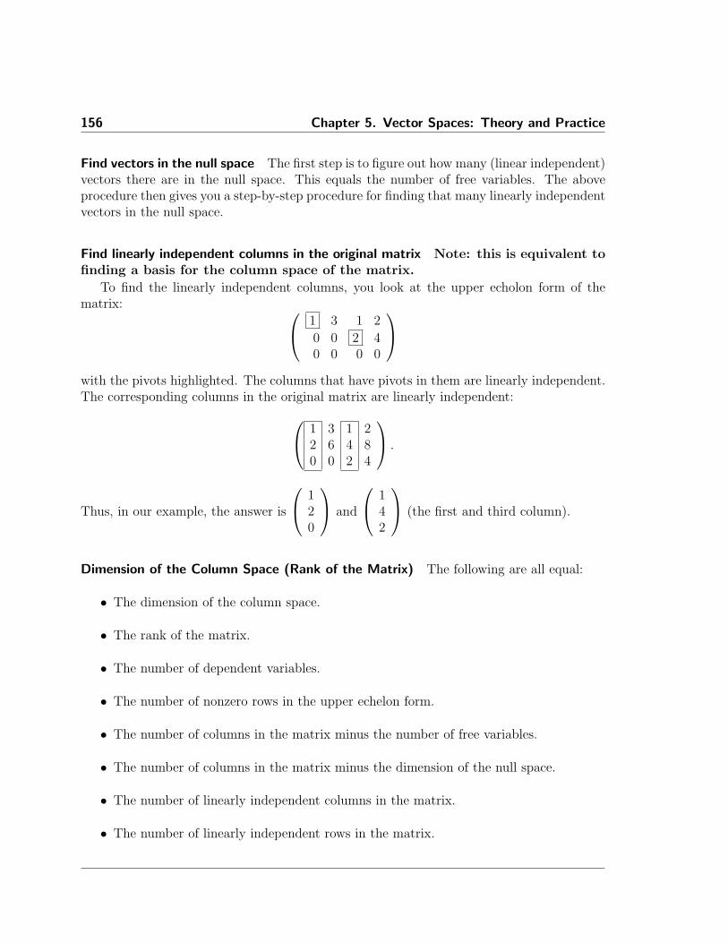
Find linearly independent columns in the original matrix Note: this is equivalent tofinding a basis for the column space of the matrix.
To find the linearly independent columns, you look at the upper echolon form of thematrix: !
#1 3 1 20 0 2 40 0 0 0
$
&
with the pivots highlighted. The columns that have pivots in them are linearly independent.The corresponding columns in the original matrix are linearly independent:
!
#1 3 1 22 6 4 80 0 2 4
$
& .
Thus, in our example, the answer is
!
#120
$
& and
!
#142
$
& (the first and third column).
Dimension of the Column Space (Rank of the Matrix) The following are all equal:
• The dimension of the column space.
• The rank of the matrix.
• The number of dependent variables.
• The number of nonzero rows in the upper echelon form.
• The number of columns in the matrix minus the number of free variables.
• The number of columns in the matrix minus the dimension of the null space.
• The number of linearly independent columns in the matrix.
• The number of linearly independent rows in the matrix.

5.6. The Answer to Life, The Universe, and Everything 157
Find a basis for the row space of the matrix. The row space (we will see in the nextchapter) is the space spanned by the rows of the matrix (viewed as column vectors). Reducinga matrix to upper echelon form merely takes linear combinations of the rows of the matrix.What this means is that the space spanned by the rows of the original matrix is the samespace as is spanned by the rows of the matrix in upper echolon form. Thus, all you need todo is list the rows in the matrix in upper echolon form, as column vectors.
For our example this means a basis for the row space of the matrix is given by
!
""#
1312
$
%%&
and
!
""#
0024
$
%%&.