Vector spaces and signal space - MIT OpenCourseWare · PDF fileChapter 5 Vector spaces and...

Chapter 5

Vector spaces and signal space

In the previous chapter, we showed that any L2 function u(t) can be expanded in various orthogonal expansions, using such sets of orthogonal functions as the T -spaced truncated sinusoids or the sinc-weighted sinusoids. Thus u(t) may be specified (up to L2 equivalence) by a countably infinite sequence such as {uk,m; −∞ < k, m < ∞} of coefficients in such an expansion.

In engineering, n-tuples of numbers are often referred to as vectors, and the use of vector notation is very helpful in manipulating these n-tuples. The collection of n-tuples of real numbers is called Rn and that of complex numbers Cn. It turns out that the most important properties of these n-tuples also apply to countably infinite sequences of real or complex numbers. It should not be surprising, after the results of the previous sections, that these properties also apply to L2

waveforms.

A vector space is essentially a collection of objects (such as the collection of real n-tuples) along with a set of rules for manipulating those objects. There is a set of axioms describing precisely how these objects and rules work. Any properties that follow from those axioms must then apply to any vector space, i.e., any set of objects satisfying those axioms. Rn and Cn satisfy these axioms, and we will see that countable sequences and L2 waveforms also satisfy them.

Fortunately, it is just as easy to develop the general properties of vector spaces from these axioms as it is to develop specific properties for the special case of Rn or Cn (although we will constantly use Rn and Cn as examples). Fortunately also, we can use the example of Rn (and particularly R2) to develop geometric insight about general vector spaces.

The collection of L2 functions, viewed as a vector space, will be called signal space. The signal-space viewpoint has been one of the foundations of modern digital communication theory since its popularization in the classic text of Wozencraft and Jacobs[35].

The signal-space viewpoint has the following merits:

• Many insights about waveforms (signals) and signal sets do not depend on time and frequency (as does the development up until now), but depend only on vector relationships.

• Orthogonal expansions are best viewed in vector space terms.

• Questions of limits and approximation are often easily treated in vector space terms. It is for this reason that many of the results in Chapter 4 are proved here.

141

Cite as: Robert Gallager, course materials for 6.450 Principles of Digital Communications I, Fall 2006. MIT OpenCourseWare(http://ocw.mit.edu/), Massachusetts Institute of Technology. Downloaded on [DD Month YYYY].

142 CHAPTER 5. VECTOR SPACES AND SIGNAL SPACE

5.1 The axioms and basic properties of vector spaces

A vector space V is a set of elements, v ∈ V, called vectors, along with a set of rules for operating on both these vectors and a set of ancillary elements called scalars. For the treatment here, the set F of scalars1 will either be the set of real numbers R or the set of complex numbers C. A vector space with real scalars is called a real vector space, and one with complex scalars is called a complex vector space.

The most familiar example of a real vector space is Rn . Here the vectors are represented as n-tuples of real numbers.2 R2 is represented geometrically by a plane, and the vectors in R2 by points in the plane. Similarly, R3 is represented geometrically by three-dimensional Euclidean space.

The most familiar example of a complex vector space is Cn, the set of n-tuples of complex numbers.

The axioms of a vector space V are listed below; they apply to arbitrary vector spaces, and in particular to the real and complex vector spaces of interest here.

1. Addition: For each v ∈ V and u ∈ V, there is a unique vector v + u ∈ V, called the sum of v and u , satisfying (a) Commutativity: v + u = u + v , (b) Associativity: v + (u + w) = (v + u) + w for each v ,u ,w ∈ V. (c) Zero: There is a unique element 0 ∈ V satisfying v + 0 = v for all v ∈ V, (d) Negation: For each v ∈ V, there is a unique −v ∈ V such that v + (−v) = 0.

2. Scalar multiplication: For each scalar3 α and each v ∈ V there is a unique vector αv ∈ Vcalled the scalar product of α and v satisfying (a) Scalar associativity: α(βv) = (αβ)v for all scalars α, β, and all v ∈ V, (b) Unit multiplication: for the unit scalar 1, 1v = v for all v ∈ V.

3. Distributive laws: (a) For all scalars α and all v ,u ∈ V, α(v + u) = αv + αu ; (b) For all scalars α, β and all v ∈ V, (α + β)v = αv + βv .

Example 5.1.1. For Rn, a vector v is an n-tuple (v1, . . . , vn) of real numbers. Addition is defined by v + u = (v1+u1, . . . , vn+un). The zero vector is defined by 0 = (0, . . . , 0). The scalars α are the real numbers, and αv is defined to be (αv1, . . . , αvn). This is illustrated geometrically in Figure 5.1.1 for R2 .

Example 5.1.2. The vector space Cn is the same as Rn except that v is an n-tuple of complex numbers and the scalars are complex. Note that C2 can not be easily illustrated geometrically, since a vector in C2 is specified by 4 real numbers. The reader should verify the axioms for both Rn and Cn .

1More generally, vector spaces can be defined in which the scalars are elements of an arbitrary field. It is not necessary here to understand the general notion of a field.

2Many people prefer to define Rn as the class of real vector spaces of dimension n, but almost everyone visualizes Rn as the space of n-tuples. More importantly, the space of n-tuples will be constantly used as an example and Rn is a convenient name for it.

3Addition, subtraction, multiplication, and division between scalars is done according to the familiar rules of R or C and will not be restated here. Neither R nor C includes ∞.

Cite as: Robert Gallager, course materials for 6.450 Principles of Digital Communications I, Fall 2006. MIT OpenCourseWare (http://ocw.mit.edu/), Massachusetts Institute of Technology. Downloaded on [DD Month YYYY].

��

� �

�

�

� � �

5.1. THE AXIOMS AND BASIC PROPERTIES OF VECTOR SPACES 143

��u Vectors are represented by

��

�w = u−v points or directed lines.

� �� The scalar multiple αu and u

αu��αw

� v

lie on the same line from 0. �� The distributive law says

��

��

��

��

��

v2 that triangles scale correctly.�� αv

0 v1

Figure 5.1: Geometric interpretation of R2. The vector v = (v1, v2) is represented as a point in the Euclidean plane with abscissa v1 and ordinate v2. It can also be viewed as the directed line from 0 to the point v . Sometimes, as in the case of w = u − v , a vector is viewed as a directed line from some nonzero point (v in this case) to another point u . This geometric interpretation also suggests the concepts of length and angle, which are not included in the axioms. This is discussed more fully later.

Example 5.1.3. There is a trivial vector space for which the only element is the zero vector 0. Both for real and complex scalars, α0 = 0. The vector spaces of interest here are non-trivial spaces, i.e., spaces with more than one element, and this will usually be assumed without further mention.

Because of the commutative and associative axioms, we see that a finite sum j αj v j , where each αj is a scalar and v j a vector, is unambiguously defined without the need for parentheses. This sum is called a linear combination of the vectors {v i}. We next show that the set of finite-energy complex waveforms can be viewed as a complex vector space.4 When we view a waveform v(t) as a vector, we denote it by v . There are two reasons for this: first, it reminds us that we are viewing the waveform is a vector; second, v(t) sometimes denotes a function and sometimes denotes the value of that function at a particular argument t. Denoting the function as v avoids this ambiguity.

The vector sum v + u is defined in the obvious way as the waveform for which each t is mapped into v(t) + u(t); the scalar product αv is defined as the waveform for which each t is mapped into αv(t). The vector 0 is defined as the waveform that maps each t into 0.

The vector space axioms are not difficult to verify for this space of waveforms. To show that the sum v + u of two finite energy waveforms v and u also has finite energy, recall first that the sum of two measurable waveforms is also measurable. Next, recall that if v and u are complex numbers, then |v + u|2 ≤ 2|v|2 + 2|u|2. Thus,

∞ ∞ ∞

|v(t) + u(t)|2 dt ≤ 2|v(t)|2 dt + 2|u(t)|2 dt < ∞. (5.1) −∞ −∞ −∞

Similarly, if v has finite energy, then αv has |α|2 times the energy of v which is also finite. The other axioms can be verified by inspection.

The above argument has shown that the set of finite-energy waveforms, along with the definitions of addiition and complex scalar multiplication, form a complex vector space. The set of real

4There is a small but important technical difference between the vector space being defined here and what we will later define to be the vector space L2. This difference centers on the notion of L2 equivalence, and will be discussed later.


�

� �

�

�


finite-energy waveforms along with the analogous addition and real scalar multiplication form a real vector space.

5.1.1 Finite-dimensional vector spaces

A set of vectors v1, . . . , vn ∈ V spans V (and is called a spanning set of V) if every vector nv∈ V is a linear combination of v1, . . . , vn. For the R example, let e1 = (1, 0, 0, . . . , 0),

ne2 = (0, 1, 0, . . . , 0), . . . , en = (0, . . . 0, 1) be the n unit vectors of Rn. The unit vectors span Rsince every vector v ∈ Rn can be expressed as a linear combination of the unit vectors, i.e.,

n

v = (α1, . . . , αn) = αj ej . j=1

A vector space V is finite-dimensional if a finite set of vectors u1, . . . ,un exist that span V. Thus Rn is finite-dimensional since it is spanned by e1, . . . , en. Similarly, Cn is finite-dimensional. If V is not finite-dimensional, then it is infinite-dimensional ; we will soon see that L2 is infinite-dimensional.

A set of vectors, v1, . . . , vn ∈ V is linearly dependent if n αjv j = 0 for some set of scalars j=1

not all equal to 0. This implies that each vector vk for which αk = 0 is a linear combination of the others, i.e.,

vk = � −αj

v j . αk

j=k

A set of vectors v1, . . . , vn ∈ V is linearly independent if it is not linearly dependent, i.e., if n αjv j = 0 implies that each αj is 0. For brevity we often omit the word “linear” when we j=1

refer to independence or dependence.

It can be seen that the unit vectors e1, . . . , en, as elements of Rn, are linearly independent. Similarly, they are linearly independent as elements of Cn ,

A set of vectors v1, . . . , vn ∈ V is defined to be a basis for V if the set both spans V and is linearly independent. Thus the unit vectors e1, . . . , en form a basis for Rn. Similarly, the unit vectors, as elements of Cn, form a basis for Cn .

The following theorem is both important and simple; see Exercise 5.1 or any linear algebra text for a proof.

Theorem 5.1.1 (Basis for finite-dimensional vector space). Let V be a non-trivial finite-dimensional vector space.5 Then

• If v1, . . . , vm span V but are linearly dependent, then a subset of v1, . . . , vm forms a basis for V with n < m vectors.

• If v1, . . . , vm are linearly independent but do not span V, then there exists a basis for Vwith n > m vectors that includes v1, . . . , vm.

• Every basis of V contains the same number of vectors. 5The trivial vector space whose only element is 0 is conventionally called a zero-dimensional space and could

be viewed as having an empty basis.


�

�

5.2. INNER PRODUCT SPACES 145

The dimension of a finite-dimensional vector space may now be defined as the number of vectors in a basis. The theorem implicitly provides two conceptual algorithms for finding a basis. First, start with any linearly independent set (such as a single nonzero vector) and successively add independent vectors until reaching a spanning set. Second, start with any spanning set and successively eliminate dependent vectors until reaching a linearly independent set.

Given any basis, v1, . . . , vn, for a finite-dimensional vector space V, any vector v ∈ V can be represented as

n

v = αj v j , where α1, . . . , αn are scalars. (5.2) j=1

In terms of the given basis, each v ∈ V can be uniquely represented by the n-tuple of coefficients (α1, . . . , αn) in (5.2). Thus any n-dimensional vector space V over R or C may be viewed (relative to a given basis) as a version6 of Rn or Cn. This leads to the elementary vector/matrix approach to linear algebra. What is gained by the axiomatic (“coordinate-free”) approach is the ability to think about vectors without first specifying a basis. We see the value of this shortly when we define subspaces and look at finite-dimensional subspaces of infinite-dimensional vector spaces such as L2.

5.2 Inner product spaces

The vector space axioms above contain no inherent notion of length or angle, although such geometric properties are clearly present in Figure 5.1.1 and in our intuitive view of Rn or Cn . The missing ingredient is that of an inner product.

An inner product on a complex vector space V is a complex-valued function of two vectors, v ,u ∈ V, denoted by 〈v ,u〉, that satisfies the following axioms:

(a) Hermitian symmetry: 〈v ,u〉 = 〈u , v〉∗; (b) Hermitian bilinearity: 〈αv + βu ,w〉 = α〈v ,w〉 + β〈u ,w〉

(and consequently 〈v , αu + βw〉 = α∗〈v ,u〉 + β∗〈v ,w〉);(c) Strict positivity: 〈v , v〉 ≥ 0, with equality if and only if v = 0.

A vector space with an inner product satisfying these axioms is called an inner product space.

The same definition applies to a real vector space, but the inner product is always real and the complex conjugates can be omitted.

The norm or length ‖v‖ of a vector v in an inner product space is defined as

.‖v‖ = 〈v , v〉

Two vectors v and u are defined to be orthogonal if 〈v,u〉 = 0. Thus we see that the important geometric notions of length and orthogonality are both defined in terms of the inner product.

6More precisely V and Rn (Cn) are isomorphic in the sense that that there is a one-to one correspondence between vectors in V and n-tuples in Rn (Cn) that preserves the vector space operations. In plain English, solvable problems concerning vectors in V can always be solved by first translating to n-tuples in a basis and then working in Rn or Cn .


�

��

� ��

�


5.2.1 The inner product spaces Rn and Cn

For the vector space Rn of real n-tuples, the inner product of vectors v = (v1, . . . vn) and u = (u1, . . . , un) is usually defined (and is defined here) as

n

〈v ,u〉 = vj uj . j=1

You should verify that this definition satisfies the inner product axioms above.

The length ‖v‖ of a vector v is then j vj 2, which agrees with Euclidean geometry. Recall

that the formula for the cosine between two arbitrary nonzero vectors in R2 is given by

cos(∠(v ,u)) = � v1u1 + � v2u2 = 〈v ,u〉

, (5.3) v1

2 + v22 u1

2 + u12 ‖v‖ ‖u‖

where the final equality also expresses this as an inner product. Thus the inner product determines the angle between vectors in R2 . This same inner product formula will soon be seen to be valid in any real vector space, and the derivation is much simpler in the coordinate free environment of general vector spaces than in the unit vector context of R2 .

For the vector space Cn of complex n-tuples, the inner product is defined as

n

〈v ,u〉 = vj uj∗ (5.4)

j=1

The norm, or length, of v is then |vj |2 = [�(vj )2 + �(vj )2]. Thus, as far as length is j j

concerned, a complex n-tuple u can be regarded as the real 2n-vector formed from the real and imaginary parts of u . Warning: although a complex n-tuple can be viewed as a real 2n−tuple for some purposes, such as length, many other operations on complex n-tuples are very different from those operations on the corresponding real 2n-tuple. For example, scalar multiplication and inner products in Cn are very different from those operations in R2n .

5.2.2 One-dimensional projections

An important problem in constructing orthogonal expansions is that of breaking a vector v into two components relative to another vector u = 0 in the same inner-product space. One component, v⊥u , is to be orthogonal (i.e., perpendicular) to u and the other, v |u , is to be collinear with u (two vectors v |u and u are collinear if v |u = αu for some scalar α). Figure 5.2 illustrates this decomposition for vectors in R2 . We can view this geometrically as dropping a perpendicular from v to u . From the geometry of Figure 5.2, ‖v |u‖ = ‖v‖ cos(∠(v ,u)). Using (5.3), ‖v |u‖ = 〈v ,u〉/‖u‖. Since v | is also collinear with u , it can be seen that u

v = 〈v ,u〉

u . (5.5)|u ‖u‖2

The vector v |u is called the projection of v onto u .

Rather surprisingly, (5.5) is valid for any inner product space. The general proof that follows is also simpler than the derivation of (5.3) and (5.5) using plane geometry.


��

��

��

� �

� ��

�

�

‖


v = (v1, v2) ��u = (u1, u2)

� v�⊥u

u2

� v |u

0 u1

Figure 5.2: Two vectors, v = (v1, v2) and u = (u1, u2) in R2 . Note that ‖u‖2 = 〈u ,u〉 = u1

2 + u22 is the squared length of u . The vector v is also expressed as v = v |u + v⊥u where

v |u is collinear with u and v⊥u is perpendicular to u .

Theorem 5.2.1 (One-dimensional projection theorem). Let v and u be arbitrary vectors with u = 0 in a real or complex inner product space. Then there is a unique scalar α for which 〈v − αu

�,u〉 = 0. That α is given by α = 〈v,u〉/‖u‖2 .

Remark: The theorem states that v −αu is perpendicular to u if and only if α = 〈v ,u〉/‖u‖2 . Using that value of α, v − αu is called the perpendicular to u and is denoted as v ; similarly αu is called the projection of v on u and is denoted as u |u . Finally, v = v⊥u + v

⊥|u

u , so v has been split into a perpendicular part and a collinear part.

Proof: Calculating 〈v − αu ,u〉 for an arbitrary scalar α, the conditions can be found under which this inner product is zero:

,〈v − αu ,u〉 = 〈v ,u〉 − α〈u ,u〉 = 〈v ,u〉 − α‖u‖2

which is equal to zero if and only if α = 〈v ,u〉/‖u‖2 .

The reason why ‖u‖2 is in the denominator of the projection formula can be understood by rewriting (5.5) as

u u v v , .|u = 〈 ‖u‖〉 ‖u‖

In words, the projection of v on u is the same as the projection of v on the normalized version of u . More generally, the value of v |u is invariant to scale changes in u , i.e.,

v |βu = 〈‖v

β

, β

u‖u2

〉βu =

〈vu

,

‖u2

〉u = v |u . (5.6)

This is clearly consistent with the geometric picture in Figure 5.2 for R2, but it is also valid for complex vector spaces where such figures cannot be drawn.

In R2, the cosine formula can be rewritten as

cos(∠(u , v)) = 〈 u ,

v . (5.7) ‖u‖ ‖v‖〉

That is, the cosine of ∠(u , v) is the inner product of the normalized versions of u and v .

Another well known result in R2 that carries over to any inner product space is the Pythagorean theorem: If v and u are orthogonal, then

‖v + u‖2 = ‖v‖2 + ‖u‖2 . (5.8)


��

��

�


To see this, note that

〈v + u , v + u〉 = 〈v , v〉 + 〈v , u〉 + 〈u , v〉 + 〈u , u〉.

The cross terms disappear by orthogonality, yielding (5.8).

Theorem 5.2.1 has an important corollary, called the Schwarz inequality :

Corollary 5.2.1 (Schwarz inequality). Let v and u be vectors in a real or complex innerproduct space. Then

|〈v, u〉| ≤ ‖v‖ ‖u‖. (5.9)

Proof: Assume u =� 0 since (5.9) is obvious otherwise. Since v |u and v⊥u are orthogonal, (5.8) shows that

‖v‖2 = ‖v |u‖2 + ‖v⊥u‖2 .

Since ‖v⊥u‖2 is nonnegative, we have

=2 2〈v , u〉

2 =

|〈v , u〉|‖u‖2

2 2 2‖v‖ ≥ ‖v |u‖ ‖u‖ ,‖u‖

which is equivalent to (5.9).

For v and u both nonzero, the Schwarz inequality may be rewritten in the form

v u,〈‖v‖ ‖u‖〉 ≤ 1.

In R2, the Schwarz inequality is thus equivalent to the familiar fact that the cosine function isupperbounded by 1.

As shown in Exercise 5.6, the triangle inequality below is a simple consequence of the Schwarzinequality.

‖v + u‖ ≤ ‖v‖ + ‖u‖. (5.10)

5.2.3 The inner product space of L2 functions

Consider the set of complex finite energy waveforms again. We attempt to define the inner product of two vectors v and u in this set as

∞

v(t)u∗(t)dt. (5.11)〈v , u〉 = −∞

It is shown in Exercise 5.8 that 〈v , u〉 is always finite. The Schwarz inequality cannot be used to prove this, since we have not yet shown that this satisfies the axioms of an inner product space. However, the first two inner product axioms follow immediately from the existence and finiteness of the inner product, i.e., the integral in (5.11). This existence and finiteness is a vital and useful property of L2.

The final inner product axiom is that 〈v , v〉 ≥ 0, with equality if and only if v = 0. This axiom does not hold for finite-energy waveforms, because as we have already seen, if a function v(t) is



zero almost everywhere, then its energy is 0, even though the function is not the zero function. This is a nit-picking issue at some level, but axioms cannot be ignored simply because they are inconvenient.

The resolution of this problem is to define equality in an L2 inner product space as L2-equivalence between L2 functions. What this means is that each element of an L2 inner product space is the equivalence class of L2 functions that are equal almost everywhere. For example, the zero equivalence class is the class of zero-energy functions, since each is L2 equivalent to the all-zero function. With this modification, the inner product axioms all hold.

Viewing a vector as an equivalence class of L2 functions seems very abstract and strange at first. From an engineering perspective, however, the notion that all zero-energy functions are the same is more natural than the notion that two functions that differ in only a few isolated points should be regarded as different.

From a more practical viewpoint, it will be seen later that L2 functions (in this equivlence class sense) can be represented by the coefficients in any orthogonal expansion whose elements span the L2 space. Two ordinary functions have the same coefficients in such an orthogonal expansion if and only if they are L2 equivalent. Thus each element u of the L2 inner product space is in one-to-one correspondence to a finite-energy sequence {uk; k ∈ Z} of coefficients in an orthogonal expansion. Thus we can now avoid the awkwardness of having many L2 equivalent ordinary functions map into a single sequence of coefficients and having no very good way of going back from sequence to function. Once again engineering common sense and sophisticated mathematics come together.

From now on we will simply view L2 as an inner product space, referring to the notion of L2

equivalence only when necessary. With this understanding, we can use all the machinery of inner product spaces, including projections and the Schwarz inequality.

5.2.4 Subspaces of inner product spaces

A subspace S of a vector space V is a subset of the vectors in V which forms a vector space in its own right (over the same set of scalars as used by V). An equivalent definition is that for all v and u ∈ S, the linear combination αv + βu is in S for all scalars α and β. If V is an inner product space, then it can be seen that S is also an inner product space using the same inner product definition as V.

Example 5.2.1 (Subspaces of R3). Consider the real inner product space R3, namely the inner product space of real 3-tuples v = (v1, v2, v3). Geometrically, we regard this as a space in which there are three orthogonal coordinate directions, defined by the three unit vectors e1, e2, e3. The 3-tuple v1, v2, v3 then specifies the length of v in each of those directions, so that v = v1e1 + v2e2 + v3e3.

Let u = (1, 0, 1) and w = (0, 1, 1) be two fixed vectors, and consider the subspace of R3 composed of all linear combinations, v = αu + βw , of u and w . Geometrically, this subspace is a plane going through the points 0,u , and w . In this plane, as in the original vector space, u and w each have length

√2 and 〈u ,w〉 = 1.

Since neither u nor w is a scalar multiple of the other, they are linearly independent. Theyspan S by definition, so S is a two-dimensional subspace with a basis {u ,w}.The projection of u on w is u |w = (0, 1/2, 1/2), and the perpendicular is u⊥w = (1,−1/2, 1/2).


�


These vectors form an orthogonal basis for S. Using these vectors as an orthogonal basis, we can view S, pictorially and geometrically, in just the same way as we view vectors in R2 .

Example 5.2.2 (General 2D subspace). Let V be an arbitrary non-trivial real or complex inner product space, and let u and w be arbitrary noncollinear vectors. Then the set S of linear combinations of u and w is a two-dimensional subspace of V with basis {u ,w}. Again, u |w

and u⊥w forms an orthogonal basis of S. We will soon see that this procedure for generating subspaces and orthogonal bases from two vectors in an arbitrary inner product space can be generalized to orthogonal bases for subspaces of arbitrary dimension.

Example 5.2.3 (R2 is a subset but not a subspace of C2). Consider the complex vector space C2 . The set of real 2-tuples is a subset of C2, but this subset is not closed under multiplication by scalars in C. For example, the real 2-tuple u = (1, 2) is an element of C2 but the scalar product iu is the vector (i, 2i), which is not a real 2-tuple. More generally, the notion of linear combination (which is at the heart of both the use and theory of vector spaces) depends on what the scalars are.

We cannot avoid dealing with both complex and real L2 waveforms without enormously complicating the subject (as a simple example, consider using the sine and cosine forms of the Fourier transform and series). We also cannot avoid inner product spaces without great complication. Finally we cannot avoid going back and forth between complex and real L2 waveforms. The price of this is frequent confusion between real and complex scalars. The reader is advised to use considerable caution with linear combinations and to be very clear about whether real or complex scalars are involved.

5.3 Orthonormal bases and the projection theorem

In an inner product space, a set of vectors φ1, φ2, . . . is orthonormal if

0 for j = k 〈φj , φk〉 = 1 for j =

�k.

(5.12)

In other words, an orthonormal set is a set of nonzero orthogonal vectors where each vector is normalized to unit length. It can be seen that if a set of vectors u1,u2, . . . is orthogonal, then the set

1 φj = uj‖uj ‖

is orthonormal. Note that if two nonzero vectors are orthogonal, then any scaling (including normalization) of each vector maintains orthogonality.

If a vector v is projected onto a normalized vector φ, then the one-dimensional projection theorem states that the projection is given by the simple formula

v |φ = 〈v , φ〉φ. (5.13)

Furthermore, the theorem asserts that v⊥φ = v −v |φ is orthogonal to φ. We now generalize the Projection Theorem to the projection of a vector v ∈ V onto any finite dimensional subspace Sof V.


�

�

� �

� = 〈

� � � �

5.3. ORTHONORMAL BASES AND THE PROJECTION THEOREM 151

5.3.1 Finite-dimensional projections

If S is a subspace of an inner product space V, and v ∈ V, then a projection of v on S is defined to be a vector v |S ∈ S such that v −v |S is orthogonal to all vectors in S. The theorem to follow shows that v always exists and has a unique value given in the theorem. |S

The earlier definition of projection is a special case of that here in which S is taken to be the one dimensional subspace spanned by a vector u (the orthonormal basis is then φ = u/‖u‖). Theorem 5.3.1 (Projection theorem). Let S be an n-dimensional subspace of an inner product space V and assume that {φ1,φ2, . . . ,φn} is an orthonormal basis for S. Then for any v ∈ V, there is a unique vector v|S ∈ S such that 〈v − v|S , s〉 = 0 for all s ∈ S. Furthermore, v is given by |S

n

v|S = 〈v, φj 〉φj . (5.14) j=1

Remark: The theorem assumes that S has a set of orthonormal vectors as a basis. It will be shown later that any non-trivial finite-dimensional inner product space has such an orthonormal basis, so that the assumption does not restrict the generality of the theorem.

Proof: Let w = n αjφj be an arbitrary vector in S. First consider the conditions on wj=1

under which v −w is orthogonal to all vectors s ∈ S. It can be seen that v −w is orthogonal to all s ∈ S if and only if

〈v −w , φj 〉 = 0, for all j, 1 ≤ j ≤ n,

or equivalently if and only if

〈v ,φj 〉 = 〈w , φj 〉, for all j, 1 ≤ j ≤ n. (5.15)

Since w = n=1 αφ ,

n

〈w , φj 〉 = α〈φ, φj 〉 = αj , for all j, 1 ≤ j ≤ n. (5.16) =1

Combining this with (5.15), v −w is orthogonal to all s ∈ S if and only if αj v , φj 〉 for each j, i.e., if and only if w = j 〈v , φj 〉φj . Thus v |S as given in (5.14) is the unique vector w ∈ Sfor which v − v |S is orthogonal to all s ∈ S.

The vector v −v |S is denoted as v⊥S , the perpendicular from v to S. Since v |S ∈ S, we see that v and v are orthogonal. The theorem then asserts that v can be uniquely split into two |S ⊥Sorthogonal components, v = v + v where the projection v is in S and the perpendicular v is orthogonal to all vectors

|Ss ∈ S

⊥S

. |S

⊥S

5.3.2 Corollaries of the projection theorem

There are three important corollaries of the projection theorem that involve the norm of the projection. First, for any scalars α1, . . . , αn, the squared norm of w = j αj φj is given by

n n n

‖w‖2 = 〈w , αj φj 〉 = αj∗〈w , φj 〉 = |αj |2 ,

j=1 j=1 j=1


�

�


where (5.16) has been used in the last step. For the projection v |S , αj = 〈v , φj 〉, so

n

‖v |S ‖2 = |〈v , φj 〉|2 . (5.17) j=1

Also, since v = v +v and v is orthogonal to v , It follows from the Pythagorean theorem |S ⊥S |S ⊥S(5.8) that

‖v‖2 = ‖v |S ‖2 + ‖v⊥S ‖2 . (5.18)

Since ‖v⊥S ‖2 ≥ 0, the following corollary has been proven:

Corollary 5.3.1 (norm bound).

0 ≤ ‖v|S ‖2 ≤ ‖ 2 , (5.19)v‖

with equality on the right if and only if v ∈ S and equality on the left if and only if v is orthogonal to all vectors in S.

Substituting (5.17) into (5.19), we get Bessel’s inequality, which is the key to understanding the convergence of orthonormal expansions.

Corollary 5.3.2 (Bessel’s inequality). Let S ⊆ V be the subspace spanned by the set of orthonormal vectors {φ1, . . . ,φn}. For any v ∈ V

n

,0 ≤ |〈v, φj 〉|2 ≤ ‖v‖2

j=1

with equality on the right if and only if v ∈ S and equality on the left if and only if v is orthogonal to all vectors in S.

Another useful characterization of the projection v |S is that it is the vector in S that is closest to v . In other words, using some s ∈ S as an approximation to v , the squared error is ‖v − s‖2 . The following corollary says that v |S is the choice for s that yields the least squared error (LS).

Corollary 5.3.3 (LS error property). The projection v|S is the unique closest vector in Sto v; i.e., for all s ∈ S,

2 2 ,‖v − v|S ‖ ≤ ‖v − s‖with equality if and only if s = v|S .

Proof: Decomposing v into v |S + v⊥S , we have v − s = [v |S − s] + v⊥S . Since v |S and s are in S, v |S − s is also in S, so by Pythagoras,

‖v − s‖2 = ‖v |S − s‖2 + ‖v⊥S ‖2 ≥ ‖v⊥S ‖2 ,

with equality if and only if ‖v |S − s‖2 = 0, i.e., if and only if s = v |S . Since v⊥S = v − vthis completes the proof.

|S ,


�


5.3.3 Gram-Schmidt orthonormalization

Theorem 5.3.1, the projection theorem, assumed an orthonormal basis {φ1, . . . ,φn} for any given n-dimensional subspace S of V. The use of orthonormal bases simplifies almost everything concerning inner product spaces, and for infinite-dimensional expansions, orthonormal bases are even more useful.

This section presents the Gram-Schmidt procedure, which, starting from an arbitrary basis {s1, . . . , sn} for an n-dimensional inner product subspace S, generates an orthonormal basis for S. The procedure is useful in finding orthonormal bases, but is even more useful theoretically, since it shows that such bases always exist. In particular, since every n-dimensional subspace contains an orthonormal basis, the projection theorem holds for each such subspace.

The procedure is almost obvious in view of the previous subsections. First an orthonormal basis, φ1 = s1/‖s1‖, is found for the one-dimensional subspace S1 spanned by s1. Projecting s2 onto this one-dimensional subspace, a second orthonormal vector can be found. Iterating, a complete orthonormal basis can be constructed.

In more detail, let (s2)|S1 be the projection of s2 onto S1. Since s2 and s1 are linearly indepen

dent, (s2)⊥S1 = s2 − (s2)|S1 is nonzero. It is orthogonal to φ1 since φ1 ∈ S1. It is normalized

as φ2 = (s2)⊥S1/‖(s2)⊥S1‖. Then φ1 and φ2 span the space S2 spanned by s1 and s2.

Now, using induction, suppose that an orthonormal basis {φ1, . . . ,φk} has been constructed for the subspace Sk spanned by {s1, . . . , sk}. The result of projecting sk+1 onto Sk is (sk+1) = �k

|Sk

j=1〈sk+1, φj 〉φj . The perpendicular, (sk+1)⊥Sk = sk+1 − (sk+1)|Sk is given by

k

(sk+1)⊥Sk = sk+1 − 〈sk+1,φj〉φj . (5.20) j=1

This is nonzero since sk+1 is not in Sk and thus not a linear combination of φ1, . . . ,φk. Normalizing,

φk+1 =(sk+1)⊥Sk (5.21) ‖( sk+1)⊥Sk ‖

From (5.20) and (5.21), sk+1 is a linear combination of φ1, . . . ,φk+1 and s1, . . . , sk are linear combinations of φ1, . . . ,φk, so φ1, . . . ,φk+1 is an orthonormal basis for the space Sk+1 spanned by s1, . . . , sk+1.

In summary, given any n-dimensional subspace S with a basis {s1, . . . , sn}, the Gram-Schmidt orthonormalization procedure produces an orthonormal basis {φ1, . . . ,φn} for S.

Note that if a set of vectors is not necessarily independent, then the procedure will automatically find any vector sj that is a linear combination of previous vectors via the projection theorem. It can then simply discard such a vector and proceed. Consequently it will still find an orthonormal basis, possibly of reduced size, for the space spanned by the original vector set.

5.3.4 Orthonormal expansions in L2

The background has now been developed to understand countable orthonormal expansions in L2. We have already looked at a number of orthogonal expansions, such as those used in the


� �

�

�

� �

� �


sampling theorem, the Fourier series, and the T -spaced truncated or sinc-weighted sinusoids. Turning these into orthonormal expansions involves only minor scaling changes.

The Fourier series will be used both to illustrate these changes and as an example of a general orthonormal expansion. The vector space view will then allow us to understand the Fourier series at a deeper level. Define θk(t) = e2πikt/T rect( t ) for k ∈ Z. The set {θk(t); k ∈ Z} ofT functions is orthogonal with ‖θk‖2 = T . The corresponding orthonormal expansion is obtained by scaling each θk by 1/T ; i.e.,

φk(t) = 1

e 2πikt/T rect( t ). (5.22)

T T

The Fourier series of an L2 function {v(t) : [−T/2, T/2] C} then becomes αkφk(t) where � → k αk = v(t)φk

∗(t) dt = 〈v ,φk〉. For any integer n > 0, let Sn be the (2n+1)-dimensional subspace spanned by the vectors {φk,−n ≤ k ≤ n}. From the projection theorem, the projection v |Sn of v on Sn is

n

v |Sn = 〈v , φk〉φk. k=−n

That is, the projection v is simply the approximation to v resulting from truncating the |Sn

expansion to −n ≤ k ≤ n. The error in the approximation, v⊥Sn = v − v |Sn , is orthogonal to all vectors in Sn, and from the LS error property, v |Sn is the closest point in Sn to v . As n increases, the subspace Sn becomes larger and v |Sn gets closer to v (i.e., ‖v − v |Sn ‖ is nonincreasing).

As the analysis above applies equally well to any orthonormal sequence of functions, the general case can now be considered. The main result of interest is the following infinite-dimensional generalization of the projection theorem.

Theorem 5.3.2 (Infinite-dimensional projection). Let {φ , 1≤m<∞} be a sequence of m

orthonormal vectors in L2, and let v be an arbitrary L2 vector. Then there exists a unique7 L2

vector u such that v − u is orthogonal to each φ andm

n

lim αmφm‖ = 0 where αm = 〈v,φm〉 (5.23) n→∞

‖u − m=1

2 2‖u‖ = |αm| . (5.24)

Conversely, for any complex sequence {αm; 1≤m≤∞} such that |αk|2 < ∞, an L2 functionk u exists satisfying (5.23) and (5.24)

Remark: This theorem says that the orthonormal expansion αmφ converges in the L2m m sense to an L2 function u , which we later interpret as the projection of v onto the infinite-dimensional subspace S spanned by {φm, 1≤m<∞}. For example, in the Fourier series case, the orthonormal functions span the subspace of L2 functions time-limited to [−T/2, T/2], and u is then v(t) rect( t ). The difference v(t)−v(t) rect( t ) is then L2 equivalent to 0 over [−T/2, T/2]T T and thus orthogonal to each φm.

7Recall that the vectors in the L2 class of functions are equivalence classes, so this uniqueness specifies only the equivalence class and not an individual function within that class.


�

� �

� �

�


Proof: Let Sn be the subspace spanned by {φ1, . . . ,�φn}. From the finite-dimensional projection theorem, the projection of v on S is then v |Sn = n αkφk. From (5.17), n k=1

n

‖v |Sn ‖2 = |αk|2 where αk = 〈v , φk〉. (5.25) k=1

This quantity is nondecreasing with n, and from Bessel’s inequality, it is upperbounded by ‖v‖2 , which is finite since v is L2. It follows that for any n and any m > n,

v = αk αkn→∞ (5.26)‖ |Sm − v |Sn ‖2 | |2 ≤ | |2 −→ 0.

n<|k|≤m |k|>n

This says that the projections {v ; n ∈ Z+} approach each other as n → ∞ in terms of their energy difference.

|Sn

A sequence whose terms approach each other is called a Cauchy sequence. The Riesz-Fischer theorem8 is a central theorem of analysis stating that any Cauchy sequence of L2 waveforms has an L2 limit. Taking u to be this L2 limit, i.e., u = l.i.m. v , we have (5.23) and (5.24).9

n→∞ |Sn

Essentially the same use of the Riesz-Fischer theorem establishes (5.23) and (5.24) starting with the sequence α1, α2, . . . .

Let S be the space of functions (or, more precisely, of equivalence classes) that can be represented as l.i.m. αkφk(t) over all sequences α1, α2, . . . such that |αk|2 < ∞. It can be seen that k k this is an inner product space. It is the space spanned by the orthonormal sequence {φk; k ∈ Z}. The following proof of the Fourier series theorem illustrates the use of the infinite dimensional projection theorem and infinite dimensional spanning sets.

Proof of Theorem 4.4.1: Let {v(t) : [−T/2, T/2]] C} be an arbitrary L2 function over →1

� [−T/2, T/2]. We have already seen that v(t) is L1, that vk = v(t)e−2πikt/T dt exists and � T that ˆ v(t) dt for all k ∈ Z. From Theorem 5.3.2, there is an L function u(t) =� 2|vk| ≤ | |

2πikt/T rect(t/T ) for l.i.m. vke2πikt/T rect(t/T ) such that v(t) − u(t) is orthogonal to θk(t) = ek

each k ∈ Z.

We now need an additional basic fact:10 the above set of orthogonal functions {θk(t) = e2πikt/T rect(t/T ); k ∈ Z} span the space of L2 functions over [−T/2, T/2], i.e., there is no function of positive energy over [−T/2, T/2] that is orthogonal to each θk(t). Using this fact, v(t) − u(t) has zero energy and is equal to 0 a.e. Thus v(t) = l.i.m. ˆ 2πikt/T rect(t/T ). The k vkeenergy equation then follows from (5.24). The final part of the theorem follows from the final part of Theorem 5.3.2.

As seen by the above proof, the infinite dimensional projection theorem can provide simple and intuitive proofs and interpretations of limiting arguments and the approximations suggested by those limits. The appendix uses this theorem to prove both parts of the Plancherel theorem, the sampling theorem, and the aliasing theorem.

Another, more pragmatic, use of the theorem lies in providing a uniform way to treat all orthonormal expansions. As in the above Fourier series proof, though, the theorem doesn’t nec

8See any text on real and complex analysis, such as Rudin[26]. 9An inner product space in which all Cauchy sequences have limits is said to be complete, and is called a

Hilbert space. Thus the Riesz-Fischer theorem states that L2 is a Hilbert space.10Again, see any basic text on real and complex analysis.



essarily provide a simple characterization of the space spanned by the orthonormal set. Fortunately, however, knowing that the truncated sinusoids span [−T/2, T/2] shows us, by duality, that the T-spaced sinc functions span the space of baseband-limited L2 functions. Similarly, both the T -spaced truncated and the sinc-weighted sinusoids span all of L2.

5.4 Summary

The theory of L2 waveforms, viewed as vectors in the inner product space known as signal space, has been developed. The most important consequence of this viewpoint is that all orthonormal expansions in L2 may be viewed in a common framework. The Fourier series is simply one example.

Another important consequence is that, as additional terms are added to a partial orthonormal expansion of an L2 waveform, the partial expansion changes by increasingly small amounts, approaching a limit in L2. A major reason for restricting attention to finite-energy waveforms (in addition to physical reality) is that as their energy gets used up in different degrees of freedom (i.e., expansion coefficients), there is less energy available for other degrees of freedom, so that some sort of convergence must result. The L2 limit above simply make this intuition precise.

Another consequence is the realization that if L2 functions are represented by orthonormal expansions, or approximated by partial orthonormal expansions, then there is no further need to deal with sophisticated mathematical issues such as L2 equivalence. Of course, how the truncated expansions converge may be tricky mathematically, but the truncated expansions themselves are very simple and friendly.

5A Appendix: Supplementary material and proofs

The first part of the appendix uses the inner-product results of this chapter to prove the theorems about Fourier transforms in Chapter 4. The second part uses inner-products to prove the theorems in Chapter 4 about sampling and aliasing. The final part discusses prolate spheroidal waveforms; these provide additional insight about the degrees of freedom in a time/bandwidth region.

5A.1 The Plancherel theorem

Proof of Theorem 4.5.1 (Plancherel 1): The idea of the proof is to expand the time-waveform u into an orthonormal expansion for which the partial sums have known Fourier transforms; the L2 limit of these transforms is then identified as the L2 transform u of u .

First expand an arbitrary L2 function u(t) in the T -spaced truncated sinusoid expansion, using T = 1. This expansion spans L2 and the orthogonal functions e2πiktrect(t− m) are orthonormal


� �

� �

� �

� �

5A. APPENDIX: SUPPLEMENTARY MATERIAL AND PROOFS 157

since T = 1. Thus the infinite dimensional projection, as specified by Theorem 5.3.2, is11

n n

u(t) = l.i.m. u(n)(t) where u(n)(t) = uk,mθk,m(t), n→∞ � m=−n k=−n

θk,m(t) = e 2πiktrect(t − m) and uk,m = u(t)θ∗ (t) dt.k,m

Since u(n)(t) is time-limited, it is L1, and thus has a continuous Fourier transform which is defined pointwise by

n n

u(n)(f) = uk,mψk,m(f), (5.27) m=−n k=−n

where ψk,m(f) = e2πifmsinc(f − k) is the k,m term of the T -spaced sinc-weighted orthonormal set with T = 1. By the final part of Theorem 5.3.2, the sequence of vectors u (n) converges to an L2 vector u (equivalence class of functions) denoted as the Fourier transform of u(t) and satisfying

lim u − u (n)‖ = 0. (5.28) n→∞

‖ˆ

This must now be related to the functions uA(t) and uA(f) in the theorem. First, for each integer > n define

n

u(n,)(f) = uk,mψk,m(f), (5.29) m=−n k=−

Since this is a more complete partial expansion than u(n)(f),

‖u − ˆ (n) u − ˆ (n,)u u‖ ≥ ‖ˆ ‖

In the limit → ∞, u (n,) is the Fourier transform uA(f) of uA(t) for A = n + 1 . Combining 2this with (5.28),

lim u n→∞

‖u − ˆn+ 1 2‖ = 0. (5.30)

Finally, taking the limit of the finite dimensional energy equation,

n n

‖u (n)‖2 = |uk,m|2 = ‖u (n)‖2 , k=−n m=−n

we get the L2 energy equation, ‖u‖2 = ‖u‖2. This also shows that ‖u − uA‖ is monotonic in A so that (5.30) can be replaced by

lim u A→∞

‖u − ˆn+ 1 2‖ = 0.

11Note that {θk,m; k, m ∈ Z} is a countable set of orthonormal vectors, and they have been arranged in an order so that, for all n ∈ Z+, all terms with |k| ≤ n and |m| ≤ n come before all other terms.


� �

�


Proof of Theorem 4.5.2 (Plancherel 2): By time/frequency duality with Theorem 4.5.1, we see that l.i.m.B→∞uB (t) exists and we denote this by F−1(u(f)). The only remaining thing to prove is that this inverse transform is L2 equivalent to the original u(t). Note first that the Fourier transform of θ0,0(t) = rect(t) is sinc(f) and that the inverse transform, defined as above, is L2 equivalent to rect(t). By time and frequency shifts, we see that u(n)(t) is the inverse transform, defined as above, of u(n)(f). It follows that limn→∞ ‖F−1(u) − u (n)‖ = 0, so we see that ‖F−1(u) − u‖ = 0.

As an example of the Plancherel theorem, let h(t) be 1 on the rationals in (0, 1) and be zero elsewhere. Then h is both L1 and L2 and has a Fourier transform h(f) = 0 which is continuous, L1, and L2. The inverse transform is also 0 and equal to h(t) a.e.

The function h(t) above is in some sense trivial since it is L2 equivalent to the zero function. The next example to be discussed is L2, nonzero only on and L1, but all members of its equivalence class are discontinuous everywhere and unbounded in every interval.

We now discuss an example of a real L2 function that is nonzero only on the interval (0, 1). This function is L1, has a continuous Fourier transform, but all functions in its equivalence class are discontinuous everywhere and unbounded over every open interval within (0, 1). This example will illustrate how truly Bizarre functions can have nice Fourier transforms and vice versa. It will also be used later to illustrate some properties of L2 functions.

Example 5A.1 (A Bizarre L2 and L1 function)). List the rationals in (0,1) by increasing denominator, i.e., as a1=1/2, a2=1/3, a3=2/3, a4=1/4, a5=3/4, a6=1/5, . Define · · ·

1 for an ≤ t < an + 2−n−1

gn(t) = 0 elsewhere,

∞g(t) = gn(t).

n=1

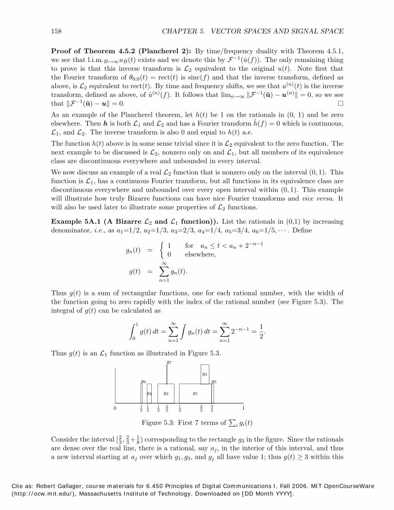
Thus g(t) is a sum of rectangular functions, one for each rational number, with the width of the function going to zero rapidly with the index of the rational number (see Figure 5.3). The integral of g(t) can be calculated as � 1 � � �∞ ∞ 1

g(t) dt = gn(t) dt = 2−n−1 = .20 n=1 n=1

Thus g(t) is an L1 function as illustrated in Figure 5.3.

g1g2

g3

g4

g5g6

g7

0 3 4

2 3

1 2

2 5

1 3

1 4

1 5

1

Figure 5.3: First 7 terms of i gi(t)

Consider the interval [23 , 32 + 18) corresponding to the rectangle g3 in the figure. Since the rationals

are dense over the real line, there is a rational, say aj , in the interior of this interval, and thus a new interval starting at aj over which g1, g3, and gj all have value 1; thus g(t) ≥ 3 within this


� � � � � � �


new interval. Moreover, this same argument can be repeated within this new interval, which again contains a rational, say aj′ . Thus there is an interval starting at aj′ where g1, g3, gj , and gj′ are 1 and thus g(t) ≥ 4.

Iterating this argument, we see that [23 , 23 + 18) contains subintervals within which g(t) takes on arbitrarily large values. In fact, by taking the limit a1, a3, aj , aj′ , . . . , we find a limit point a for which g(a) = ∞. Moreover, we can apply the same argument to any open interval within (0, 1) to show that g(t) takes on infinite values within that interval.12 More explicitly, for every ε > 0 and every t ∈ (0, 1), there is a t′ such that |t − t′| < ε and g(t′) = ∞. This means that g(t) is discontinuous and unbounded in each region of (0, 1).

The function g(t) is also in L2 as seen below: � 1 � � g 2(t) dt = gn(t)gm(t) dt (5.31)

0 n,m

∞= gn

2(t) dt + 2 gn(t) gm(t) dt (5.32) n n m=n+1

1 ∞ � 3 ≤

2 + 2 gm(t) dt =

2, (5.33)

n m=n+1

where in (5.33) we have used the fact that gn2(t) = gn(t) in the first term and gn(t) ≤ 1 in the

second term.

In conclusion, g(t) is both L1 and L2 but is discontinuous everywhere and takes on infinite values at points in every interval. The transform g(f) is continuous and L2 but not L1. The inverse transform, gB (t) of g(f)rect( f ) is continuous, and converges in L2 to g(t) as B → ∞. For 2B B = 2k, the function gB (t) is roughly approximated by g1(t)+ +gk(t), all somewhat rounded · · ·at the edges.

This is a nice example of a continuous function g(f) which has a bizarre inverse Fourier transform. Note that g(t) and the function h(t) that is 1 on the rationals in (0,1)and 0 elsewhere are both discontinuous everywhere in (0,1). However, the function h(t) is 0 a.e., and thus is weird only in an artificial sense. For most purposes, it is the same as the zero function. The function g(t) is weird in a more fundamental sense. It cannot be made respectable by changing it on a countable set of points.

One should not conclude from this example that intuition cannot be trusted, or that it is necessary to take a few graduate math courses before feeling comfortable with functions. One can conclude, however, that the simplicity of the results about Fourier transforms and orthonormal expansions for L2 functions is truly extraordinary in view of the bizarre functions included in the L2 class.

In summary, Plancherel’s theorem has taught us two things. First, Fourier transforms and inverse transforms exist for all L2 functions. Second, finite-interval and finite-bandwidth approximations become arbitrarily good (in the sense of L2 convergence) as the interval or the bandwidth becomes large.

12The careful reader will observe that g(t) is not really a function R R, but rather a function from R to the →extended set of real values including ∞ and −∞. The set of t on which g(t) = ∞ has zero measure and this can be ignored in Lebesgue integration. Do not confuse a function that takes on an infinite value at some isolated point with a unit impulse at that point. The first integrates to 0 around the singularity, whereas the second is a generalized function that by definition integrates to 1.


� � �

�

()

�

�


5A.2 The sampling and aliasing theorems

This section contains proofs of the sampling and aliasing theorems. The proofs are important and not available elsewhere in this form. However, they involve some careful mathematical analysis that might be beyond the interest and/or background of many students.

Proof of Theorem 4.6.2 (Sampling Theorem): Let u (f ) be an L2 function that is zero outside of [−W, W]. From Theorem 4.3.2, u (f ) is L1, so by Lemma 4.5.1, � W

u (t ) = u(f )e 2πift df (5.34) −W

holds at each t ∈ R. We want to show that the sampling theorem expansion also holds at each t . By the DTFT theorem,

u(f ) = l. i. m. u()(f ), where u()(f ) = u kφk(f ) (5.35) →∞

k=−

and where φk(f ) = e −2πikf/(2W)rect 2f W and

1 � W

u k = u(f )e 2πikf/(2W) df. (5.36)2W −W

Comparing (5.34) and (5.36), we see as before that 2Wu k = u (2k W). The functions φk(f ) are in

L1, so the finite sum u ()(f ) is also in L1. Thus the inverse Fourier transform

� k u ()(t ) = u()(f ) df = u ( ) sinc(2Wt − k )

2Wk=−

is defined pointwise at each t . For each t ∈ R, the difference u (t ) − u ()(t ) is then � W

u (t ) − u ()(t ) = [u (f ) − u()(f )]e 2πift df. −W

This integral can be viewed as the inner product of u (f ) − u()(f ) and e −2πiftrect[ f ], so, by 2Wthe Schwarz inequality, we have

|u (t ) − u ()(t )| ≤√

2W‖u − u ‖.

From the L2 convergence of the DTFT, the right side approaches 0 as → ∞, so the left side also approaches 0 for each t , establishing pointwise convergence.

Proof of Theorem 4.6.3 (Sampling theorem for transmission): For a given W, assume that the sequence {u (2

k W); k ∈ Z} satisfies k |u (2

k W)|2 < ∞. Define u k = 2

1 Wu (2

k W) for each

k ∈ Z. By the DTFT theorem, there is a frequency function u (f ), nonzero only over [−W, W], that satisfies (4.60) and (4.61). By the sampling theorem, the inverse transform u (t ) of u (f ) has the desired properties.

Proof of Theorem 4.7.1 (Aliasing theorem): We start by separating u (f ) into frequency slices {vm(f ); m ∈ Z},

u(f ) = vm(f ), where vm(f ) = u (f )rect†(fT − m ). (5.37) m


� �

�

��

�

��

� �


The function rect†(f) is defined to equal 1 for −1 < f ≤ 1 and 0 elsewhere. It is L2 equivalent 2 2

to rect(f), but gives us pointwise equality in (5.37). For each positive integer n, define v(n)(f) as

n

v(n)(f) = vm(f) = u(f) for 2n−1 < f ≤ 2n+1

2T elsewhere.

(5.38)2T 0

m=−n

It is shown in Exercise 5.16 that the given conditions on u(f) imply that u(f) is in L1. In conjunction with (5.38), this implies that

∞

u(f) − v(n)(f)lim |df = 0.|n→∞ −∞

(n)(f) is in L1, the inverse transform at each t satisfies

∞

Since u(f) − v

(n)(t) (n)(f)]e 2πift dfu(t) − v [u(f) − ˆ= v−∞∞

u(f) − v(n)(f) df = u(f) df.≤ | ||f |≥(2n+1)/(2T )−∞

Since u(f) is in L1, the final integral above approaches 0 with increasing n. Thus, for each t, we have

u(t) = lim v(n)(t). (5.39) n→∞

Next define sm(f) as the frequency slice vm(f) shifted down to baseband, i.e.,

m m sm(f) = vm(f − ) = u(f − )rect†(fT ). (5.40)

T T

Applying the sampling theorem to vm(t), we get

T

t − k)e 2πimt/T . (5.41)(t) = vm(kT ) sinc( vm

k

Applying the frequency shift relation to (5.40), we see that sm(t) = vm(t)e−2πift, and thus

t T

− k).(t) = vm(kT ) sinc( (5.42)sm

k

(n)(f) = (n)(f) is the aliased version of n smNow define s (f). From (5.40), we see that sm=−n (n)(f), as illustrated in Figure 4.10. The inverse transform is then v

s∞ n

(n)(t) = vm(kT ) sinc( t T

− k). (5.43)k=−∞ m=−n

We have interchanged the order of summation, which is valid since the sum over m is finite. Finally, define s(f) to be the “folded” version of u(f) summing over all m, i.e.,

s(f) = l.i.m. s(n)(f). (5.44) n→∞


� �

�

�

�


Exercise 5.16 shows that this limit converges in the L2 sense to an L2 function s(f). Exercise 4.38 provides an example where s(f) is not in L2 if the condition lim|f |→∞ u(f)|f |1+ε = 0 is not satisfied.

Since s(f) is in L2 and is 0 outside [− 1 1 ], the sampling theorem shows that the inverse 2T , 2Ttransform s(t) satisfies � t

s(t) = s(kT )sinc(T

− k). (5.45) k

Combining this with (5.43),

n� � t s(t) − s(n)(t) = s(kT ) − vm(kT ) sinc(

T − k). (5.46)

k m=−n

From (5.44), we see that limn→∞ ‖s − s(n)‖ = 0, and thus

lim s(kT ) − v(n)(kT ) 2 = 0. n→∞

k

| |

This implies that s(kT ) = limn→∞ v(n)(kT ) for each integer k. From (5.39), we also have

u(kT ) = limn→∞ v(n)(kT ), and thus s(kT ) = u(kT ) for each k ∈ Z. � t

s(t) = u(kT )sinc(T

− k). (5.47) k

This shows that (5.44) implies (5.47). Since s(t) is in L2, it follows that k |u(kT )|2 < ∞. Conversely, (5.47) defines a unique L2 function, and thus its Fourier transform must be L2

equivalent to s(f) as defined in (5.44).

5A.3 Prolate spheroidal waveforms

The prolate spheroidal waveforms (see [29]) are a set of orthonormal functions that provide a more precise way to view the degree-of-freedom arguments of Section 4.7.2. For each choice of baseband bandwidth W and time interval [−T/2, T/2], these functions form an orthonormal set {φ0(t), φ1(t), . . . , } of real L2 functions time-limited to [−T/2, T/2]. In a sense to be described, these functions have the maximum possible energy in the frequency band (−W, W) subject to their constraint to [−T/2, T/2].

To be more precise, for each n ≥ 0 let φn(f) be the Fourier transform of φn(t), and define

θn(f) = �

φn(f) for − W<t<W (5.48)0 elsewhere.

That is, θn(t) is φn(t) truncated in frequency to (−W, W); equivalently, θn(t) may be viewed as the result of passing φn(t) through an ideal low-pass filter.

The function φ0(t) is chosen to be the normalized function φ0(t) : (−T/2, T/2) → R that maximizes the energy in θ0(t). We will not show how to solve this optimization problem. However, φ0(t) turns out to resemble 1/T rect(T

t ), except that it is rounded at the edges to reduce the out-of-band energy.


�


Similarly, for each n > 0, the function φn(t) is chosen to be the normalized function {φn(t) : (−T/2, T/2) → R} that is orthonormal to φm(t) for each m < n and, subject to this constraint, maximizes the energy in θn(t).

Finally, define λn = ‖θn‖2 . It can be shown that 1 > λ0 > λ1 > . We interpret λn as the · · · fraction of energy in φ that is baseband-limited to (−W,W). The number of degrees of freedom n in (−T/2, T/2), (−W, W) is then reasonably defined as the largest n for which λn is close to 1.

The values λn depend on the product TW, so they can be denoted by λn(TW). The main result about prolate spheroidal wave functions, which we do not prove, is that for any ε > 0,

1 for n < 2TW(1 − ε)lim λn(TW) =

0 for n > 2TW(1 + ε).T W→∞

This says that when TW is large, there are close to 2TW orthonormal functions for which most of the energy in the time-limited function is also frequency-limited, but there are not significantly more orthonormal functions with this property.

The prolate spheroidal wave functions φn(t) have many other remarkable properties, of which we list a few:

• For each n, φn(t) is continuous and has n zero crossings.

• φn(t) is even for n even and odd for n odd.

• θn(t) is an orthogonal set of functions.

• In the interval (−T/2, T/2), θn(t) = λnφn(t).


�

�

�


5.E Exercises

5.1. (basis) Prove Theorem 5.1.1 by first suggesting an algorithm that establishes the first item and then an algorithm to establish the second item.

5.2. Show that the 0 vector can be part of a spanning set but cannot be part of a linearly indepenendent set.

5.3. (basis) Prove that if a set of n vectors uniquely spans a vector space V, in the sense that each v ∈ V has a unique representation as a linear combination of the n vectors, then those n vectors are linearly independent and V is an n-dimensional space.

5.4. (R2) (a) Show that the vector space R2 with vectors {v = (v1, v2)} and inner product 〈v ,u〉 = v1u1 + v2u2 satisfies the axioms of an inner product space. (b) Show that, in the Euclidean plane, the length of v (i.e., the distance from 0 to v is ‖v‖. (c) Show that the distance from v to u is ‖v − u‖. (d) Show that cos(∠(v ,u)) = 〈v ,u〉 ; assume that ‖u‖ > 0 and ‖v‖ > 0.‖v‖ ‖u‖

(e) Suppose that the definition of the inner product is now changed to 〈v ,u〉 = v1u1+2v2u2. Does this still satisfy the axioms of an inner product space? Does the length formula and the angle formula still correspond to the usual Euclidean length and angle?

5.5. Consider Cn and define 〈v ,u〉 as jn =1 cjvju

∗j where c1, . . . , cn are complex numbers. For

each of the following cases, determine whether Cn must be an inner product space and explain why or why not. (a) The cj are all equal to the same positive real number. (b) The cj are all positive real numbers. (c) The cj are all non-negative real numbers. (d) The cj are all equal to the same nonzero complex number. (e) The cj are all nonzero complex numbers.

5.6. (Triangle inequality) Prove the triangle inequality, (5.10). Hint: Expand ‖v +u‖2 into four terms and use the Schwarz inequality on each of the two cross terms.

5.7. Let u and v be orthonormal vectors in Cn and let w = wuu + wvv and x = xuu + xvv be two vectors in the subspace spanned by u and v . (a) Viewing w and x as vectors in the subspace C2, find 〈w ,x 〉. (b) Now view w and x as vectors in Cn , e.g., w = (w1, . . . , wn) where wj = wuuj + wvvj

for 1 ≤ j ≤ n. Calculate 〈w ,x 〉 this way and show that the answer agrees with that in part (a).

5.8. (L2 inner product) Consider the vector space of L2 functions {u(t) : R C}. Let v and u→be two vectors in this space represented as v(t) and u(t). Let the inner product be defined by

〈v ,u〉 = ∞

v(t)u∗(t) dt. � −∞

(a) Assume that u(t) = uk,mθk,m(t) where {θk,m(t)} is an orthogonal set of functions k,m each of energy T . Assume that v(t) can be expanded similarly. Show that

〈u , v〉 = T ˆ v∗uk,mˆk,m. k,m

Cite as: Robert Gallager, course materials for 6.450 Principles of Digital Communications I, Fall 2006. MIT OpenCourseWare(http://ocw.mit.edu/), Massachusetts Institute of Technology. Downloaded on [DD Month YYYY].

� �

� | | | |

� �

5.E. EXERCISES 165

(b) Show that 〈u , v〉 is finite. Do not use the Schwarz inequality, because the purpose of this exercise is to show that L2 is an inner product space, and the Schwarz inequality is based on the assumption of an inner product space. Use the result in (a) along with the properties of complex numbers (you can use the Schwarz inequality for the one dimensional vector space C1 if you choose). (c) Why is this result necessary in showing that L2 is an inner product space?

5.9. (L2 inner product) Given two waveforms u1,u2 ∈ L2, let V be the set of all waveforms v that are equi-distant from u1 and u2. Thus

.V = v : ‖v − u1‖ = ‖v − u2‖

(a) Is V a vector sub-space of L2? (b) Show that � 2 2 �

V = v : � (〈v ,u2 − u1〉) = ‖u2‖ − ‖u1‖

.2

(c) Show that (u1 + u2)/2 ∈ V(d) Give a geometric interpretation for V.

5.10. (sampling) For any L2 function {u(t) : [−W,W] C} and any t, let ak = u( k ) and let � 2

→ � 2

2Wbk = sinc(2Wt − k). Show that k ak < ∞ and k bk < ∞. Use this to show that

k |akbk| < ∞. Use this to show that the sum in the sampling equation (4.65) converges for each t.

5.11. (projection) Consider the following set of functions {um(t)} for integer m ≥ 0:

u0(t) = 1, 0 ≤ t < 1; 0 otherwise.

. . .

um(t) = 1, 0 ≤ t < 2−m; 0 otherwise.

. . .

Consider these functions as vectors u0,u1 . . . , over real L2 vector space. Note that u0 is normalized; we denote it as φ0 = u0. (a) Find the projection (u1)|φ0

of u1 on φ0, find the perpendicular (u1)⊥φ0, and find the

normalized form φ1 of (u1)⊥φ0 . Sketch each of these as functions of t.

(b) Express u1(t − 1/2) as a linear combination of φ0 and φ1. Express (in words) the subspace of real L2 spanned by u1(t) and u1(t − 1/2). What is the subspace S1 of real L2

spanned by φ0 and φ1? (c) Find the projection (u2)|S1

of u2 on S1, find the perpendicular (u2)⊥S1 , and find the normalized form of (u2) . Denote this normalized form as φ2,0; it will be clear shortly ⊥S1

why a double subscript is used here. Sketch φ2,0 as a function of t. (d) Find the projection of u2(t − 1/2) on S1 and find the perpendicular u2(t − 1/2)⊥S1 . Denote the normalized form of this perpendicular by φ2,1. Sketch φ2,1 as a function of t and explain why 〈φ2,0, φ2,1〉 = 0.


� �

� � �


(e) Express u2(t − 1/4) and u2(t − 3/4) as linear combinations of {φ0, φ1, φ2,0, φ2,1}. Let S2 be the subspace of real L2 spanned by φ0,φ1, φ2,0, φ2,1 and describe this subspace in words. (f) Find the projection (u3)|S2

of u3 on S2, find the perpendicular (u2)⊥S1 , and find its normalized form, φ3,0. Sketch φ3,0 as a function of t. (g) For j = 1, 2, 3, find u3(t − j/4)⊥S2 and find its normalized form φ3,j . Describe the subspace S3 spanned by φ0,φ1, φ2,0,φ2,1, φ3,0, . . . ,φ3,3. (h) Consider iterating this process to form S4,S5, . . . . What is the dimension of Sm? Describe this subspace. Describe the projection of an arbitrary real L2 function constrained to the interval [0,1) on Sm.

5.12. (Orthogonal subspaces) For any subspace S of an inner product space V, define S⊥ as the set of vectors v ∈ V that are orthogonal to all w ∈ S. (a) Show that S⊥ is a subspace of V. (b) Assuming that S is finite dimensional, show that any u ∈ V can be uniquely decomposed into u = u |S + u⊥S where u |S ∈ S and u⊥S ∈ S⊥. (c) Assuming that V is finite dimensional, show that V has an orthonormal basis where some of the basis vectors form a basis for S and the remaining basis vectors form a basis for S⊥.

5.13. (Orthonormal expansion) Expand the function sinc(3t/2) as an orthonormal expansion in the set of functions {sinc(t − n) ; −∞ < n < ∞}.

5.14. (bizarre function) (a) Show that the pulses gn(t) in Example 5A.1 of Section 5A.1 overlap each other either completely or not at all.

n−1(b) Modify each pulse �gn(t) to hn(t) as follows: Let �hn(t) = gn(t) if i=1 gi(t) is even and n−1let hn(t) = −gn(t) if i=1 gi(t) is odd. Show that n hi(t) is bounded between 0 and 1 i=1

for each t ∈ (0, 1) and each n ≥ 1. (c) Show that there are a countably infinite number of points t at which n hn(t) does not converge.

5.15. (Parseval) Prove Parseval’s relation, (4.44) for L2 functions. Use the same argument as used to establish the energy equation in the proof of Plancherel’s theorem.

5.16. (Aliasing theorem) Assume that u(f) is L2 and lim|f |→∞ u(f)|f |1+ε = 0 for some ε > 0. (a) Show that for large enough A > 0, |u(f)| ≤ |f |−1−ε for |f | > A. � (b) Show that u(f) is L1. Hint: for the A above, split the integral |u(f)| df into one integral for |f | > A and another for |f | ≤ A. (c) Show that, for T = 1, s(f) as defined in (5.44), satisfies

|s(f)| ≤ (2A + 1) |m|≤A

|u(f + m)|2 + m≥A

m−1−ε .

(d) Show that s(f) is L2 for T = 1. Use scaling to show that s(f) is L2 for any T > 0.


Vector spaces and signal space - MIT OpenCourseWare · PDF fileChapter 5 Vector spaces and...

Documents

Transcript of Vector spaces and signal space - MIT OpenCourseWare · PDF fileChapter 5 Vector spaces and...