Vector Median Filters: A Survey - IJCSNSpaper.ijcsns.org/07_book/201612/20161210.pdf ·...

IJCSNS International Journal of Computer Science and Network Security, VOL.16 No.12, December 2016

66

Manuscript received December 5, 2016 Manuscript revised December 20, 2016

Vector Median Filters: A Survey

Roji Chanu1, and Kh. Manglem Singh2 1Department of Electronics & Communication Engineering, National Institute of Technology Nagaland

2Department of Computer Science & Engineering Engineering, National Institute of Technology Manipur

Abstract In this paper, a comprehensive survey on vector median filters to remove the adverse effect due to impulse noise from color images is presented. Color images are nonstationary vectored value signals. Hence, nonlinear filters such as vector median filters are more effective than linear filters. A number of nonlinear filters are proposed in the literature. They have been categorized into 12 groups and discussed in details. Keywords Impulse noise, Vector median filter, Quaternion, Nonlinear, Sigma vector filter, Entropy vector filter.

1. Introduction

Color images are widely used on daily basis in printing, photographs, computer displays, television and movies and thus color image processing plays a crucial role in the field of advertising and dissemination of information [1]. The use of color images is increasing in medical images and remote sensing. Color information are being used in many color image processing applications like object recognition, image matching, content-based image retrieval, computer vision, color image compression, etc. [2]. Color images are corrupted by noise due to malfunctioning of sensors, electronic interference, imperfect optics, or fault in the data transmission process. Noise introduces color fluctuation making pixel values different from the ideal values and thus produces errors which complicate the subsequent stages of the image processing process [3]. A filter transforms a signal into a more suitable form for a specific purpose [4]. Filtering gives an estimate of signal degraded by noise. Since color images are nonstationary in nature due to the presence of edges and fine details, and also the human visual system is nonlinear, nonlinear filters are preferred more than linear filters. A color image can be treated as a mapping for 2D to 3D [5]. The three color channels exhibit strong spectral correlation. Marginal or component-wise filtering methods which process each channel independently produce images containing color shifts and other serious artifacts. In vector filtering techniques the input pixels are treated as a set of vectors and no new colors are introduced. Hence theyare able to preserve the correlation among the channel components [5-8]. Thus an efficient filter aims at processing of color images with respect to its trichromatic

nature, nonlinear characteristics and noise corruption statistics. Impulse noise is a high energy spikes having large amplitude with probability greater than that predicted by Gaussian density model occurring for a short duration. It is required to remove noise in the preprocessing stage to prevent degradation of image quality.Many nonlinear filters have been proposed in the literature for removing impulse noise. In this study, a large number of nonlinear filters are categorized into 12 families. This paper aims at summarizing the recent developments in the vector median filters for removal impulse noise from color images. Section 2 describes the categories of vector median filters. In Section 3, a commonly used impulse noise model is described. Popular filtering performance criteria for evaluation filters are given in Section 4 followed by conclusion in Section 5.

2. Category of Filters

In this section, the commonly used filters used for removing impulse noise are grouped into 12 categories. They are

1. Basic Vector Filters 2. Weighted Vector Filters 3. Adaptive Vector Filters 4. Peer Group Vector Filters 5. Fuzzy Vector Filters 6. Hybrid Vector Filters 7. Sigma Vector Filters 8. EntropyVector Filters 9. Quaternion based Vector Filters 10. Morphological based vector median filters 11. Wavelet based median filters 12. Miscellaneous Filters

2.1 BasicVector Filters

The reduced vector or aggregated ordering technique is the most common filtering approach. In this method the aggregated distance of a sample pixel 𝒙𝒙𝑖𝑖 inside a sliding filtering window 𝑊𝑊 of length N, usually a finite odd number, is computed as follows:

IJCSNS International Journal of Computer Science and Network Security, VOL.16 No.12, December 2016 67

𝐷𝐷𝑖𝑖 = ∑ 𝜌𝜌𝒙𝒙𝑖𝑖 ,𝒙𝒙𝑗𝑗, 𝑖𝑖 = 1, … ,𝑁𝑁𝑁𝑁𝑗𝑗=1 (1)

in which ρ(.) represents the distance or dissimilarity function, 𝒙𝒙𝑖𝑖 =(𝑥𝑥𝑖𝑖1 , 𝑥𝑥𝑖𝑖2, 𝑥𝑥𝑖𝑖3) and 𝒙𝒙𝑗𝑗=(𝑥𝑥𝑗𝑗1, 𝑥𝑥𝑗𝑗2, 𝑥𝑥𝑗𝑗3) for three channels. The sorting of aggregated distance 𝑠𝑠 𝐷𝐷1,𝐷𝐷2 … ,𝐷𝐷𝑁𝑁 in ascending order represents same ordering of the associated vectors 𝐷𝐷(1) ≤ 𝐷𝐷(2) ≤ ⋯ ≤ 𝐷𝐷(𝑁𝑁) ⇒ 𝒙𝒙(1) ≤ 𝒙𝒙(2) ≤ ⋯ ≤ 𝒙𝒙(𝑁𝑁) (2)

2.1.1 Vector Median Filter (VMF)

In [9] Vector Median filter (VMF), Generalized Vector Median Filter (GVMF) and Extended Vector Median Filter (EVMF) are introduced for processing vector-valued signals having properties similar with median filters operation such as zero impulse response and good smoothing ability while preserving sharp edges in the signal. They are based on the concept of nonlinear order statistics and derived as maximum likelihood estimates from exponential distributions. Since vectors which vary greatly from the data population correspond to the maximum aggregated magnitude difference, the VMF output is the lowest ranked vector with minimum aggregated distance to the input vectors present inside the window. If 𝒙𝒙1, … ,𝒙𝒙𝑁𝑁 represent the vectors inside the filtering window W, the vector median is computed as follows: a) For each vector element 𝒙𝒙𝑖𝑖 calculate the sum of distances to all other vectors inside the filtering window, using the Minkowski metric (either the 𝐿𝐿1or 𝐿𝐿2 norm) and add them together to get sum of distances 𝑆𝑆𝑖𝑖 𝑆𝑆𝑖𝑖 = ∑ 𝒙𝒙𝑖𝑖 − 𝒙𝒙𝑗𝑗𝛾𝛾

𝑁𝑁𝑗𝑗=1 (3)

where 𝛾𝛾 = 1 for city block distance and 𝛾𝛾 = 2 for Euclidean distance. b) Find a parameter 𝑚𝑚𝑖𝑖𝑚𝑚 such that 𝑆𝑆𝑚𝑚𝑖𝑖𝑚𝑚 denotes the minimum 𝑆𝑆𝑖𝑖 . c) Corresponding to 𝑆𝑆𝑚𝑚𝑖𝑖𝑚𝑚 , 𝒙𝒙𝑚𝑚𝑖𝑖𝑚𝑚 = 𝒙𝒙(1) represents the vector median 𝒙𝒙𝑉𝑉𝑉𝑉𝑉𝑉.

2.1.2 α-trimmed Vector Median Filter (α-VMF)

In α-VMF a trimming operation is incorporated in which (1+α) nearest samples to the vector median are given as input to an average filter. The output is defined as follows [9, 10]: 𝒙𝒙αVMF = ∑ 1

(1+𝛼𝛼)1+𝛼𝛼𝑖𝑖=1 𝒙𝒙𝑖𝑖 , 𝛼𝛼 ∈ [0,𝑁𝑁 − 1] (4)

The trimming operation enhances in removing the long tailed or impulsive noise while the averaging filter performs well with Gaussian noise.

2.1.3 Extended Vector Median Filter (EXVMF)

EXVMF combines the vector median operation with an averaging filter. EXVMF of 𝒙𝒙𝑖𝑖 , …𝒙𝒙𝑁𝑁 is denoted as 𝒙𝒙𝐸𝐸𝐸𝐸𝑉𝑉𝑉𝑉𝑉𝑉 such that [9, 10] 𝒙𝒙𝐸𝐸𝐸𝐸𝑉𝑉𝑉𝑉𝑉𝑉 =

𝒙𝒙𝐴𝐴𝑉𝑉𝐸𝐸 , 𝑖𝑖𝑖𝑖 ∑ ∥ 𝒙𝒙𝐴𝐴𝑉𝑉𝐸𝐸 − 𝒙𝒙𝑖𝑖 ∥2 < ∑ ∥ 𝒙𝒙𝑉𝑉𝑉𝑉𝑉𝑉 − 𝒙𝒙𝑖𝑖 ∥2 𝑁𝑁𝑖𝑖=1

𝑁𝑁𝑖𝑖=1

𝒙𝒙𝑉𝑉𝑉𝑉𝑉𝑉 , otherwise (5)

where 𝒙𝒙𝐴𝐴𝑉𝑉𝐸𝐸 = 1

𝑁𝑁∑ 𝒙𝒙𝑖𝑖𝑁𝑁𝑖𝑖=1 and 𝒙𝒙𝑉𝑉𝑉𝑉𝑉𝑉 is the vector median

output. It behaves like VMF near the edges while in smooth areas it behaves like the Arithmetic Mean Filter (AMF).

2.1.4 Generalized Vector Median Filter (GVMF)

The GVMF [11] of vectors 𝒙𝒙𝑖𝑖 , … 𝒙𝒙𝑁𝑁 is vector 𝒙𝒙𝐺𝐺𝑉𝑉𝑉𝑉𝑉𝑉 such that 𝒙𝒙𝐺𝐺𝑉𝑉𝑉𝑉𝑉𝑉 ∈ 𝑥𝑥𝑖𝑖 ∣∣ 𝑖𝑖 = 1, … ,𝑁𝑁 and for all 𝑗𝑗 = 1, … ,𝑁𝑁 satisfying the condition ∑ 𝑑𝑑(𝒙𝒙𝐺𝐺𝑉𝑉𝑉𝑉𝑉𝑉 − 𝒙𝒙𝑖𝑖)𝑁𝑁𝑖𝑖=1 ≤ ∑ 𝑑𝑑(𝒙𝒙𝑗𝑗 − 𝒙𝒙𝑖𝑖)𝑁𝑁

𝑖𝑖=1 (6) where 𝑑𝑑(𝒙𝒙,𝒚𝒚) is the distance between the vectors 𝒙𝒙 and 𝒚𝒚.

2.1.5 Fast Modified Vector Median Filter (FMVMF)

In [12] a new filter similar with VMF is developed whose computational complexity is lower than that of VMF. The distance associated with central pixel 𝒙𝒙𝑁𝑁+1

2 is denoted by

𝑑𝑑(𝑁𝑁+1)/2 = −𝛽𝛽 + (∑ 𝑑𝑑(𝒙𝒙𝑁𝑁+12

,𝒙𝒙𝑗𝑗)𝑁𝑁+12 −1𝑗𝑗=1 +

∑ 𝑑𝑑(𝒙𝒙𝑁𝑁+12

,𝒙𝒙𝑗𝑗)𝑁𝑁𝑗𝑗=𝑁𝑁+12 +1

where 𝛽𝛽 is a threshold parameter

and the distance associated with the neighbors of 𝒙𝒙𝑁𝑁+12

is

given as 𝑑𝑑𝑖𝑖 = ∑ 𝑑𝑑(𝒙𝒙𝑖𝑖 ,𝒙𝒙𝑗𝑗)𝑁𝑁𝑗𝑗=1 , 𝑖𝑖 =

1,2, 3, … ,𝑁𝑁, excluding (𝑁𝑁 + 1)/2. Then for some 𝑘𝑘, if 𝑑𝑑𝑘𝑘 is smaller than 𝑑𝑑(𝑁𝑁+1)/2 i.e. 𝑑𝑑𝑘𝑘 = ∑ 𝑑𝑑(𝒙𝒙𝑘𝑘,𝒙𝒙𝑗𝑗)𝑁𝑁

𝑗𝑗=1 <𝑑𝑑(𝑁𝑁+1)/2, then 𝒙𝒙𝑁𝑁+1

2 is replaced by 𝒙𝒙𝑘𝑘.

2.1.6 Directional Vector Median Filter (DVMF)

In this filter, four vector median are applied across the four main directions of the filtering window at 0°, 45°, 90°and135° to obtain four vector median output 𝒚𝒚1,𝒚𝒚2,𝒚𝒚3 and 𝒚𝒚4. In the second stage, the final output is generated by applying another vector median on the four filtered results. Hence the Directional Vector Median Filter (DVMF) output is denoted as [13] 𝒙𝒙𝐷𝐷𝑉𝑉𝑉𝑉𝑉𝑉 = 𝒚𝒚(1) (7) where 𝒚𝒚(1) is the vector median of 𝒚𝒚𝟏𝟏,𝒚𝒚2,𝒚𝒚3 and 𝒚𝒚4. DVMF is effective in removing impulsive noise while preserving thin lines.


2.1.7 Rank Conditioned Vector Median Filter (RCVMF)

It incorporates a decision making process in which every pixels in the filtering window is assigned a rank depending on the ordered distance. In RCVMF [14] the output is the vector median when the rank of central pixel is larger than a predefined rank of uncorrupted vector pixels in the filtering window. Mathematically it is denoted as

𝒙𝒙𝑅𝑅𝑅𝑅𝑉𝑉𝑉𝑉𝑉𝑉 = 𝒙𝒙𝑉𝑉𝑉𝑉𝑉𝑉 , 𝑖𝑖𝑖𝑖 𝑟𝑟(𝑁𝑁+1)/2 > 𝑟𝑟𝑘𝑘𝒙𝒙𝑁𝑁+1

2, otherwise (8)

where 𝑟𝑟(𝑁𝑁+1)/2 denotes rank of center pixel and 𝑟𝑟𝑘𝑘 is the rank of predefined healthy pixel.

2.1.8 Rank Conditioning and Threshold Vector Median Filter (RCTVMF)

In [14], a new improvement in the RCVMF is proposed in which the distance 𝑑𝑑 between the central pixel and predefined healthy pixel is used as additional criteria for impulse detection.

𝒙𝒙𝑅𝑅𝑅𝑅𝑅𝑅𝑉𝑉𝑉𝑉𝑉𝑉 = 𝒙𝒙𝑅𝑅𝑅𝑅𝑅𝑅𝑉𝑉𝑉𝑉𝑉𝑉 , 𝑖𝑖𝑖𝑖 𝑟𝑟𝑁𝑁+1

2> 𝑟𝑟𝑘𝑘 and 𝐷𝐷 > 𝑇𝑇

𝒙𝒙𝑁𝑁+12

, otherwise (9)

where 𝐷𝐷 = 𝛥𝛥(𝒙𝒙𝑁𝑁+12

,𝒙𝒙(𝑘𝑘)) denotes the distance between

central pixel and neighboring healthy pixels in which 𝒙𝒙(𝑘𝑘)(1 < 𝑘𝑘 < 𝑁𝑁) is a rank-ordered and healthy vector pixel. 𝑇𝑇 is a pre-determined threshold. If the central pixel is detected as impulse, it is replaced by the vector median output.

2.1.9 Crossing Level Median Mean Filter (CLMMF)

Crossing Level Median Mean Filter [15] combines the idea of the VMF and Arithmetic Mean Filter (AMF) which is based on the vector ordering technique. If 𝑤𝑤𝑖𝑖 denotes the weight of 𝑖𝑖𝑡𝑡ℎ elements of the ordered vectors 𝒙𝒙(1),𝒙𝒙(2), … 𝒙𝒙(𝑁𝑁), the filtered output is given as follows: 𝒙𝒙𝑅𝑅𝐶𝐶𝑉𝑉𝑉𝑉𝑉𝑉 = ∑ 𝑤𝑤(𝑖𝑖).𝒙𝒙(𝑖𝑖)

𝑁𝑁𝑖𝑖=1 (10)

where

𝑤𝑤(𝑖𝑖) = 1 − 𝑁𝑁

(𝑁𝑁+1)(𝑁𝑁+1+γ), for 𝑖𝑖 = 1

1(𝑁𝑁+1)(𝑁𝑁+1+γ)

, for 𝑖𝑖 = 2, … ,𝑁𝑁 (11)

where γ represents the parameter of the filter which resembles the standard VMF for γ→ ∞ and AMF for γ=0.

2.1.10 Vector Filters based on Non-Causal (NC) linear prediction technique

A group of switching filters based on noncausal linear prediction is introduced in [16]. NC gives an estimate of

the current pixel based on the past and future pixel values in the neighborhood of the current pixel by using a block-by-block autocorrelation function. The difference between the predicted pixel and the original current pixel is used as a measure for impulse detection. The predicted pixel value at central location ( 𝑟𝑟, 𝑐𝑐 ) is computed as 𝒙𝒙(𝑟𝑟, 𝑐𝑐) = ∑ 𝑎𝑎(𝑖𝑖, 𝑗𝑗).𝒙𝒙(𝑟𝑟 − 𝑖𝑖, 𝑐𝑐 − 𝑗𝑗) = 𝜲𝜲𝜂𝜂𝒂𝒂𝜂𝜂(𝑖𝑖,𝑗𝑗)∈𝑊𝑊2 (12) where 𝒂𝒂𝜂𝜂 represents the vector obtained from the prediction coefficients, 𝑊𝑊2 is the noncausal region for linear prediction, 𝜲𝜲𝜂𝜂 denotes the matrix of vector pixels used for prediction and 𝜂𝜂 is the order of prediction. Then the predictor decides if the current sample is corrupted or not and is replaced by the vector median if the predicted error 𝑒𝑒(𝑟𝑟, 𝑐𝑐) exceeds a pre-defined threshold 𝑇𝑇. Hence the output of the noncausal linear prediction based vector filter 𝒙𝒙𝑁𝑁𝑅𝑅𝑉𝑉𝑉𝑉 is denoted by

𝒙𝒙𝑁𝑁𝑅𝑅𝑉𝑉𝑉𝑉 = 𝒙𝒙𝑉𝑉𝑉𝑉𝑉𝑉 , if ∥ 𝑒𝑒(𝑟𝑟, 𝑐𝑐) ∥> 𝑇𝑇𝒙𝒙(𝑟𝑟, 𝑐𝑐), otherwise (13)

2.1.11 Basic Vector Directional Filter (BVDF)

It is a rank ordered filter in which the angle between two vectors is used as the distance measure. The vectors with atypical directions are regarded as an outlier and filtering is done similar with the VMF. The aggregated sum of angles between the vectors is given by 𝜃𝜃𝑖𝑖 = ∑ 𝐴𝐴(𝒙𝒙𝑖𝑖 ,𝒙𝒙𝑗𝑗)𝑁𝑁

𝑗𝑗=1 , 𝑖𝑖 = 1, … ,𝑁𝑁 (14) where

𝐴𝐴𝒙𝒙𝑖𝑖 ,𝒙𝒙𝒋𝒋 = cos−1 𝒙𝒙𝑖𝑖.𝒙𝒙𝑗𝑗

∥𝒙𝒙𝑖𝑖∥∥𝒙𝒙𝑗𝑗∥ (15)

where 𝐴𝐴𝒙𝒙𝑖𝑖 ,𝒙𝒙𝑗𝑗 represents the angle between the vectors 𝒙𝒙𝒊𝒊 and 𝒙𝒙𝑗𝑗 . The angles are ordered which correspond to ordering of the input vectors as follows: 𝜃𝜃(1) ≤ 𝜃𝜃(2) ≤ ⋯𝜃𝜃(𝑟𝑟) … ≤ 𝜃𝜃(𝑁𝑁) → 𝒙𝒙(1) ≤ 𝒙𝒙(2) ≤ ⋯𝒙𝒙(𝑟𝑟) …

≤ 𝒙𝒙(𝑁𝑁) The output of BVDF [17] is the vector 𝒙𝒙𝑖𝑖 whose angular distance to all other vector in the window is minimum. BVDF preserves chromaticity better than the VMF since vector’s direction corresponds to its chromaticity. BVDF considers only directional processing and is effective when vector magnitudes are less important than the vectors direction which is not suitable for multichannel signal processing.

2.1.12 Generalized Vector Directional Filter (GVDF)

The above mentioned filters do not consider both the unique features of a vector namely direction and magnitude together which may produce erroneous results. GVDF [18] is a generalization of BVDF. In the first step, a set of low- rank vectors that is the first 𝑟𝑟 terms are selected from the ordered set of vectors based on the aggregated sum of angular distance as opposed to the


BVDF in which a single vector with the minimum aggregated angular sum is selected. Next these vectors are given as an input to an additional filter, e.g. alpha-trimmed average filter, multistage median filter or morphological filters which consider magnitude processing. Hence GVDF considers both the directional and magnitude processing.

2.1.13 Directional Distance Filter (DDF)

An improved filter is achieved by combining VMF and VDF which is known as Directional Distance Filter (DDF) [18,19]. DDF considers the vector’s direction and magnitude in which both the vector’s chromaticity and intensity are considered. The combined aggregated measure is defined as follows: Ω𝑖𝑖 = ∑ ∥ 𝒙𝒙𝑖𝑖 − 𝒙𝒙𝑗𝑗 ∥𝛾𝛾𝑁𝑁

𝑗𝑗=1 1−𝑝𝑝. ∑ 𝐴𝐴(𝒙𝒙𝑖𝑖 ,𝒙𝒙𝑗𝑗)𝑁𝑁𝑗𝑗=1 𝑝𝑝 (16)

where 𝑝𝑝 ∈ (0, 1) is a parameter which tunes the influence of magnitude and angle quantities.

2.1.14 Filters based on Hopfield Neural Network and Improved Vector Median Filter

In this filter, the noise detection in done using a Hopfield neural network (HNN) and in the second stage, the noisy pixels are replaced by an improved Vector Median Filter first in RGB space and then in HSI space [20]. For the improved VMF, the steps are given by

1. The vector median is computed in RGB space inside the filtering window.

2. All the pixels fit for being median inside the filtering window are collected.

3. If more than one pixel is fit for being median, then select that particular pixel which is nearest to the mean of the Hue in HSI space

4. In Step 3 if more than one pixel is qualified, then the pixel which is nearest to the mean of saturation in HSI space is selected.

2. 2 Weighted Vector Filters

Weighted Vector Filters are extension of Weighted Standard Median Filters in which a non-negative weight is assigned to every pixel inside the filtering window offering more flexibility.

2.2.1 Weighted Vector Median Filter (WVMF)

WVMF is a generalization of VMF in which each pixel 𝑥𝑥𝑖𝑖 in the filter window is assigned a positive integer weight. The weight controls the filtering behavior while offering greater flexibility than the median-based filter. If 𝒙𝒙1,𝒙𝒙2, … ,𝒙𝒙𝑁𝑁 are vectors inside the filtering window and 𝑤𝑤1,𝑤𝑤2, … ,𝑤𝑤𝑁𝑁 are the corresponding nonnegative integer-

valued weights, then WVMF is the vector 𝒙𝒙𝑊𝑊𝑉𝑉𝑉𝑉 such that [10, 21] 𝒙𝒙𝑊𝑊𝑉𝑉𝑉𝑉 ∈ 𝒙𝒙𝑖𝑖; 𝑖𝑖 = 1, … ,𝑁𝑁 and for all 𝑗𝑗 = 1, … ,𝑁𝑁 ∑ 𝑤𝑤𝑖𝑖 ∥ 𝒙𝒙𝑊𝑊𝑉𝑉𝑉𝑉 − 𝒙𝒙𝑖𝑖 ∥𝛾𝛾𝑁𝑁𝑖𝑖=1 ≤ ∑ 𝑤𝑤𝑖𝑖 ∥ 𝒙𝒙𝑗𝑗 − 𝒙𝒙𝒊𝒊 ∥𝛾𝛾𝑁𝑁

𝑖𝑖=1 (17) It can be summarized as follows: sort the pixels inside the filtering window depending on the value of vector median, duplicate each pixel 𝒙𝒙𝑖𝑖 to the number of their corresponding weight 𝑤𝑤𝑖𝑖 and the median value from the new sequence represents the weighted vector median.

2.2.2 α-Trimmed Weighted Vector Median Filter (α-TWVMF)

α-TWVMF [21] of vectors 𝒙𝒙1,𝒙𝒙2, … ,𝒙𝒙𝑵𝑵 having weights 𝑤𝑤1,𝑤𝑤2, … ,𝑤𝑤𝑁𝑁 is defined as 𝒙𝒙𝛼𝛼−𝑅𝑅𝑊𝑊𝑉𝑉𝑉𝑉 =

𝒙𝒙𝛼𝛼 , if∑ 𝑤𝑤𝑖𝑖 ∥ 𝒙𝒙𝛼𝛼 − 𝒙𝒙𝑖𝑖 ∥< ∑ 𝑤𝑤𝑖𝑖 ∥ 𝒙𝒙𝑊𝑊𝑉𝑉𝑉𝑉 − 𝒙𝒙𝑖𝑖 ∥𝑁𝑁𝑖𝑖=1

𝑁𝑁𝑖𝑖=1

𝒙𝒙𝑊𝑊𝑉𝑉𝑉𝑉 , otherwise (18)

where 𝒙𝒙𝛼𝛼 = 1∣𝑆𝑆𝛼𝛼∣

∑ 𝒙𝒙𝑖𝑖𝒙𝒙𝑖𝑖∈𝑆𝑆𝛼𝛼 and 𝑆𝑆𝛼𝛼 = 𝒙𝒙𝑖𝑖; having 𝑆𝑆𝑖𝑖 <

𝑆𝑆(𝑁𝑁−𝛼𝛼) 𝑆𝑆𝑖𝑖 is the sum of weighted from vector 𝒙𝒙𝑖𝑖 to all other vectors 𝒙𝒙𝑗𝑗, 𝑗𝑗 = 1, … ,𝑁𝑁. ∣ 𝑆𝑆𝛼𝛼 ∣ represents the number of elements in 𝑆𝑆𝛼𝛼 and 𝑆𝑆(𝑖𝑖) is the 𝑖𝑖𝑡𝑡ℎ smallest of 𝑆𝑆1, … 𝑆𝑆𝑁𝑁 . 𝛼𝛼 can have any value 0, 1, ………., N-1.

2.2.3 Extended Weighted Vector Median Filter (EXWVMF)

The EXWVMF [21,22] is an extension of WVMF which is defined as 𝒙𝒙𝐸𝐸𝐸𝐸𝑊𝑊𝑉𝑉𝑉𝑉𝑉𝑉 =

𝒙𝒙𝑊𝑊𝐴𝐴𝑉𝑉𝐸𝐸 , if ∑ 𝑤𝑤𝑖𝑖 ∥ 𝒙𝒙𝑊𝑊𝐴𝐴𝑉𝑉𝐸𝐸 − 𝒙𝒙𝑖𝑖 ∥<𝑁𝑁𝑖𝑖=1 ∑ 𝑤𝑤𝑖𝑖 ∥ 𝒙𝒙𝑊𝑊𝑉𝑉𝑉𝑉 − 𝒙𝒙𝑖𝑖 ∥𝑁𝑁

𝑖𝑖=1𝒙𝒙𝑊𝑊𝑉𝑉𝑉𝑉, otherwise

(19) where 𝒙𝒙𝑊𝑊𝐴𝐴𝑉𝑉𝐸𝐸 = 1

∑ 𝑤𝑤𝑖𝑖𝑁𝑁𝑖𝑖=1

∑ 𝑤𝑤𝑖𝑖𝒙𝒙𝑖𝑖𝑁𝑁𝑖𝑖=1 (20)

EWVMF chooses the average as output in the smooth areas while it chooses weighted vector median (WVM) near edges.

2.2.4 Rank Order Weighted Vector Median Filter (ROWVMF)

In [23] an adaptive noise attenuating and edge enhancing filter based on the minimization of aggregated weighted distances among pixels in window is proposed. The distance between a pixel 𝒙𝒙𝑖𝑖 and all other pixels inside the filtering window is ordered to obtain 𝑑𝑑𝑖𝑖(𝑟𝑟)by assigning a rank 𝑟𝑟 𝑑𝑑𝑖𝑖1,𝑑𝑑𝑖𝑖2, … ,𝑑𝑑𝑖𝑖𝑁𝑁 → 𝑑𝑑𝑖𝑖(1), 𝑑𝑑𝑖𝑖(2), … ,𝑑𝑑𝑖𝑖(𝑁𝑁) A weighted sum of distances is computed by utilizing the distance ranks denoted as follows: 𝛬𝛬𝑖𝑖 = ∑ 𝑖𝑖(𝑟𝑟).𝑑𝑑𝑖𝑖(𝑟𝑟)

𝑁𝑁𝑟𝑟=1 (21)


where 𝑖𝑖(𝑟𝑟) denotes a constantfunction associated with the distance rank 𝑟𝑟. All the weighted aggregated distances 𝛬𝛬𝑖𝑖 are sorted forming a new order of vectors 𝛬𝛬(1),𝛬𝛬(2), … ,𝛬𝛬(𝑁𝑁) → 𝒙𝒙(1)

∗ ,𝒙𝒙(2)∗ , … ,𝒙𝒙(𝑁𝑁)

∗ The output of the ROWVMF is the vector 𝒙𝒙(1)

∗ . Another filter called Rank-based Vector Median Filter having similar concept is also designed in [24].

2.2.5 Weighted Vector Directional Filters (WVDF)

It employs a nonnegative real weighing coefficient 𝑤𝑤1,𝑤𝑤2, …𝑤𝑤𝑁𝑁 corresponding to vector elements 𝒙𝒙1,𝒙𝒙2, …𝒙𝒙𝑁𝑁 with filter output 𝒙𝒙𝑊𝑊𝑉𝑉𝐷𝐷𝑉𝑉 = 𝒙𝒙𝑖𝑖 ∈ 𝑊𝑊 which minimizes the aggregated weighted angular distance with other vector pixels given by [25, 26] 𝒙𝒙𝑊𝑊𝑉𝑉𝐷𝐷𝑉𝑉 = 𝑎𝑎𝑟𝑟𝑎𝑎𝑚𝑚𝑖𝑖𝑚𝑚

𝒙𝒙𝑖𝑖∈𝑊𝑊∑ 𝑤𝑤𝑗𝑗𝐴𝐴(𝒙𝒙𝑖𝑖 ,𝒙𝒙𝑗𝑗)𝑁𝑁𝑗𝑗=1 (22)

where 𝐴𝐴(𝒙𝒙𝑖𝑖 ,𝒙𝒙𝑗𝑗) represents the angle between two vectors. Similarly Weighted Directional Distance Filter (WDDF) is also obtained using both the magnitude and angular distance criteria.

2.2.6 Genetic Algorithm based Weighted Vector Directional Filter (GA WVDF)

An optimized WVDF based on Genetic Algorithm is designed in [27] which adapts the filter weights in order to match the varying image and noise characteristics. Since GA-based methods search the entire solution space, they are able to provide a globally optimal (or very close) solution as compared with other optimization techniques. Another filter based on Genetic Programming (GP) is developed in [28] aiming at the removal of mixed noise. The estimator is based on the global learning capability of GP and measurement of local statistical properties of the healthy pixels present in the surrounding of the corrupted pixel.

2.2.7 Center-Weighted Vector Median Filter (CWVMF)

In WVMF when the center weight is varied and the others remain fixed, a new class of filter is formed called the Center weighted Vector Median Filter (CWVMF) [29,30] is formed. It is defined as 𝒙𝒙𝑅𝑅𝑊𝑊𝑉𝑉𝑉𝑉𝑉𝑉𝑘𝑘 = argmin

𝑥𝑥𝑖𝑖∈𝑊𝑊∑ 𝑤𝑤𝑗𝑗(𝑘𝑘). ∥ 𝒙𝒙𝑖𝑖 − 𝒙𝒙𝑗𝑗 ∥𝑁𝑁

𝑗𝑗=1 (23)

with 𝑤𝑤𝑗𝑗(𝑘𝑘) = 𝑁𝑁 − 2𝜅𝜅 + 2, for 𝑗𝑗 = (𝑁𝑁 + 1)/21, otherwise

where only the central weight 𝑤𝑤(𝑁𝑁+1)/2 is varied with smoothing parameter 𝜅𝜅.

2.3 Adaptive Vector Filters

VMF and its variants result in fixed amount of smoothing leading to blurring of edges and fine details since they perform filtering operation on all pixels which may not be

noisy. Also noise characteristics varies in the image and hence nonadaptive filters have low performance. Adaptive filters are introduced to handle the difficulty of varying noise characteristics by implementing estimation procedures based on the nature of data on local image statistics [3]. The coefficients of filter kernel change values depending on the image structure which is to be smoothed.

2.3.1 Adaptive Vector Median filter (AVMF)

In this filter desired features are made invariant to filtering operation while the noisy pixels are effected by altering between VMF and the identity operation. This is based on the decision rule expressed as follows [31] if 𝑉𝑉𝑎𝑎𝑉𝑉 ≥ 𝑇𝑇𝑇𝑇𝑉𝑉 , then 𝒙𝒙𝑁𝑁+1

2 is impulse

else 𝒙𝒙𝑁𝑁+12

is noise free

where 𝑉𝑉𝑎𝑎𝑉𝑉 is the vector distance between the central pixel 𝒙𝒙𝑁𝑁+1

2 and the mean of the first 𝑟𝑟 vector order statistics

𝒙𝒙(1),𝒙𝒙(2), … ,𝒙𝒙(𝑟𝑟) associated with the ordered distances 𝐿𝐿(1), 𝐿𝐿(2), … , 𝐿𝐿(𝑟𝑟) , for 𝑟𝑟 ≤ 𝑁𝑁. 𝑇𝑇𝑇𝑇𝑉𝑉 is a prespecified threshold value. Mathematically, 𝑉𝑉𝑎𝑎𝑉𝑉 is denoted by

𝑉𝑉𝑎𝑎𝑉𝑉 = 𝒙𝒙𝑁𝑁+12− 1

𝑟𝑟∑ 𝒙𝒙(𝑖𝑖)𝑟𝑟𝑖𝑖=1

𝛾𝛾 (24)

where γ characterizes the norm used in Minkowski metric. If noise is detected the central pixel is replaced by the vector median output. Another adaptive filter is the Adaptive Basic Vector Directional Filter (ABVDF) which is the angular counterpart of AVMF.

2.3.2 Adaptive based Impulsive Noise Removal Filter

In [32], a new adaptive filtering scheme is proposed. The impulse is detected based on the difference between the aggregated distance assigned to central pixel and the vector median output. The output of the filter is given as follows: 𝒙𝒙𝑜𝑜𝑜𝑜𝑡𝑡𝑝𝑝𝑜𝑜𝑡𝑡 = 𝛼𝛼𝒙𝒙𝑁𝑁+1

2+ (1 − 𝛼𝛼)𝒙𝒙(1) (25)

where 𝛼𝛼 is a filter parameter and 𝒙𝒙(1) is the VMF output. The value of 𝛼𝛼 is 0 when an impulse is present otherwise it is 1.

2.3.3 Multiclass Support Vector Machine based Adaptive Filter (MSVMAF)

A new filter called Multiclass Support Vector Machine based Adaptive Filter (MSVMAF) is developed in [33] for reducing high density impulse noise. It takes the advantages of both multiclass Support Vector Machine (SVM) as well as adaptive vector median filtering.


2.3.4 Adaptive Threshold and Color Correction (ATCC) Filter

For removing random-valued impulse noise, a new filter named Adaptive Threshold and Color Correction (ATCC) filter is proposed in [34]. It has an adaptive threshold which is computed on the basis of local pixel statistics within the sliding window.

2.3.5 Robust Switching Vector Filter (RSVF)

In this filter, the pixels in the window are ordered according to the distance measure used in VFM, VDF and DDF. A pixel is detected as corrupted if the cumulative distance 𝑑𝑑(𝑁𝑁+1)/2 of the central pixel is larger than the median cumulative distance of the neighborhood. The output of the filter is one of the outputs of VMF, VDF and DDF as follows: 𝒙𝒙𝑅𝑅𝑆𝑆𝑉𝑉𝑉𝑉 =

𝒙𝒙(𝑁𝑁+1)/2, if 𝑑𝑑(𝑁𝑁+1)/2 ≤ med 𝛼𝛼. (𝑑𝑑1, … ,𝑑𝑑𝑁𝑁) < 0𝒙𝒙𝑅𝑅𝑆𝑆𝑉𝑉𝑉𝑉 , otherwise (26)

where 𝑚𝑚𝑒𝑒𝑑𝑑(. ) is a robust univariate median operator and 𝛼𝛼 is a filter parameter used for preserving image details and smoothing. If 𝑑𝑑𝑖𝑖 = ∑ 𝐿𝐿𝛾𝛾(𝒙𝒙𝑖𝑖 ,𝒙𝒙𝑗𝑗)𝑁𝑁

𝑗𝑗=1 the output is denoted by the VMF (𝒙𝒙𝑅𝑅𝑆𝑆𝑉𝑉𝑉𝑉 = 𝒙𝒙𝑅𝑅𝑆𝑆𝑉𝑉𝑉𝑉𝑉𝑉) to obtain Robust Switching Vector Median Filter (RSVMF). If 𝑑𝑑𝑖𝑖=∑ 𝐴𝐴(𝒙𝒙𝑖𝑖 ,𝒙𝒙𝑗𝑗)𝑁𝑁

𝑗𝑗=1 , 𝒙𝒙𝑅𝑅𝑆𝑆𝑉𝑉𝑉𝑉 = 𝒙𝒙𝑅𝑅𝑆𝑆𝑅𝑅𝑉𝑉𝐷𝐷𝑉𝑉 to represent Robust Switching Basic Vector Directional Filter (RSBVDF) while for 𝑑𝑑𝑖𝑖 = (∑ 𝐴𝐴(𝒙𝒙𝑖𝑖 ,𝒙𝒙𝑗𝑗)𝑁𝑁

𝑗𝑗=1 )𝛾𝛾(∑ 𝐿𝐿𝑝𝑝(𝒙𝒙𝑖𝑖 ,𝒙𝒙𝑗𝑗))𝑁𝑁𝑗𝑗=1

1−𝛾𝛾 , 𝒙𝒙𝑅𝑅𝑆𝑆𝑉𝑉𝑉𝑉 = 𝒙𝒙𝑅𝑅𝑆𝑆𝐷𝐷𝐷𝐷𝑉𝑉 which is obtained by the Directional Distance filter output to represent Robust Switching Directional Distance filter (RSDDF) [35,36].

2.3.6 Adaptive Marginal Median filter (AMMF)

A new modification to Vector Marginal Median Filter (VMMF) is designed in [4] which aims at integrating the noise reduction capability of VMMF as well as preserving the vector correlation resulting from VMF. From the ordered aggregated distance used in VMF 𝑑𝑑(1),𝑑𝑑(2), …𝑑𝑑(𝑁𝑁) → 𝒙𝒙(1),𝒙𝒙(2), … 𝒙𝒙(𝑁𝑁) , select a set of vectors 𝑆𝑆 constituted by 𝑚𝑚 vectors which are most similar to the Vector Median 𝒙𝒙(1) such that 𝑆𝑆 =𝒙𝒙(1),𝒙𝒙(2), …𝒙𝒙(𝑚𝑚) for 𝑚𝑚 ≤ 𝑁𝑁. Then the Vector Marginal Median filter is applied to this set to achieve high noise reduction. The output of the marginal median filter is given as follows [37] 𝒙𝒙𝐴𝐴𝑉𝑉𝑉𝑉 =(𝑚𝑚𝑒𝑒𝑑𝑑(𝑥𝑥(1)

𝑅𝑅 , …𝑥𝑥(𝑁𝑁)𝑅𝑅 ), 𝑚𝑚𝑒𝑒𝑑𝑑(𝑥𝑥(1)

𝐺𝐺 , …𝑥𝑥(𝑁𝑁)𝐺𝐺 ), (𝑚𝑚𝑒𝑒𝑑𝑑(𝑥𝑥(1)

𝑅𝑅 , … 𝑥𝑥(𝑁𝑁)𝑅𝑅 )))

(27)

2.3.7 Adaptive Center-Weighted Vector Filter

To provide more flexibility for modification in the size and shape of the window, adaptive center weighted vector

filters are designed in [29,38,39]. They are based on user-defined threshold for detection of impulses. If the central pixel is detected as corrupted, it is replaced by one of the output of VMF, BVDF and DDF forming ACWVMF, ACWBVDF and ACWDDF. The mathematical expressions of the corresponding filters are given below

𝒙𝒙𝐴𝐴𝑅𝑅𝑊𝑊𝑉𝑉𝑉𝑉𝑉𝑉 = 𝒙𝒙𝑉𝑉𝑉𝑉𝑉𝑉 , if ∑ ∥ 𝒙𝒙𝑅𝑅𝑊𝑊𝑉𝑉𝑉𝑉𝑉𝑉𝑘𝑘 − 𝒙𝒙𝑁𝑁+1

2∥𝜆𝜆+2

𝑘𝑘=𝜆𝜆 > 𝑇𝑇

𝒙𝒙𝑁𝑁+12

, otherwise

(28)

𝒙𝒙𝐴𝐴𝑅𝑅𝑊𝑊𝑅𝑅𝑉𝑉𝐷𝐷𝑉𝑉 = 𝒙𝒙𝑅𝑅𝑉𝑉𝐷𝐷𝑉𝑉 , if ∑ 𝐴𝐴(𝒙𝒙𝑅𝑅𝑊𝑊𝑅𝑅𝑉𝑉𝐷𝐷𝑉𝑉𝑘𝑘 − 𝒙𝒙𝑁𝑁+1

2

𝜆𝜆+2𝑘𝑘=𝜆𝜆 ) > 𝑇𝑇

𝒙𝒙𝑁𝑁+12

, otherwise

(29) 𝒙𝒙𝐴𝐴𝑅𝑅𝑊𝑊𝐷𝐷𝐷𝐷𝑉𝑉 =

𝒙𝒙𝐷𝐷𝐷𝐷𝑉𝑉 , if ∑ 𝐴𝐴𝛾𝛾(𝒙𝒙𝑅𝑅𝑊𝑊𝐷𝐷𝐷𝐷𝑉𝑉𝑘𝑘 − 𝒙𝒙𝑁𝑁+1

2) ∥ 𝒙𝒙𝑅𝑅𝑊𝑊𝐷𝐷𝐷𝐷𝑉𝑉𝑘𝑘 − 𝒙𝒙𝑁𝑁+1

2∥1−𝛾𝛾𝜆𝜆+2

𝑘𝑘=𝜆𝜆 > 𝑇𝑇

𝒙𝒙𝑁𝑁+12

, otherwise (30)

where λ∈ [1,𝑁𝑁+12− 1]

2.3.8. Modified switching median filter (MSMF)

It is an extension of the VMF and AVMF consisting of two-stage noise detector [40]. In the first stage, the probably noisy candidates are detected using the AVMF detection procedure as follows

𝒚𝒚𝑉𝑉𝑆𝑆𝑉𝑉𝑉𝑉 = 𝒚𝒚𝑠𝑠𝑡𝑡𝑠𝑠𝑝𝑝 2𝑉𝑉𝑆𝑆𝑉𝑉𝑉𝑉 , 𝒙𝒙𝑁𝑁+1

2− 1

𝑟𝑟∑ 𝒙𝒙(𝑖𝑖)𝑟𝑟𝑖𝑖=1

𝛾𝛾≥ 𝑇𝑇𝑇𝑇𝑉𝑉

𝒙𝒙𝑁𝑁+12

, otherwise (31)

In the second phase for preserving the edge pixels, these noise candidates are again judged by four Laplacian operators in which the central pixel is convolved with four convolution kernals. For edge detection, the minimum difference of the four convolutions denoted by 𝑍𝑍 is used and the noisy samples are replaced by the VMF. The output is defined as follows:

𝒁𝒁 = min 𝒙𝒙𝑁𝑁+12∗ 𝑊𝑊𝑐𝑐| 𝑐𝑐 = 1, … ,4 (32)

𝒚𝒚𝑠𝑠𝑡𝑡𝑠𝑠𝑝𝑝2𝑉𝑉𝑆𝑆𝑉𝑉𝑉𝑉 = 𝒚𝒚𝑉𝑉𝑉𝑉𝑉𝑉 , 𝑍𝑍 ≥ 𝑇𝑇𝒙𝒙𝑁𝑁+1

2, otherwise (33)

2.3.9 Sharpening Vector Median Filter

In [23] if the function 𝑖𝑖(𝑟𝑟) is a step-like function defined by

𝑖𝑖(𝑟𝑟) = 1, for 𝑟𝑟 ≤ 𝛼𝛼 𝑎𝑎𝑚𝑚𝑑𝑑 𝛼𝛼 ≤ 𝑁𝑁0, otherwise (34)

then a new vector filter is obtained known as the Sharpening Vector Median Filter [41].


2.3.10 Adaptive rank weighted switching filter (ARWSF)

ARWSF [42] is a modification of the Rank Order Weighted Vector Median Filter which incorporates an adaptive scheme. If the rank weighted distance assigned to the central pixel 𝒙𝒙𝑁𝑁+1

2 is denoted by 𝛬𝛬𝑁𝑁+1

2, then the

difference 𝛿𝛿 = 𝛬𝛬𝑁𝑁+12− 𝛬𝛬(1) is used for measuring impulse

noise corruption. The output of ARWSF is given as follows:

𝒚𝒚𝐴𝐴𝑅𝑅𝑊𝑊𝑆𝑆𝑉𝑉 = 𝒙𝒙𝐴𝐴𝑉𝑉𝑉𝑉 , if 𝛿𝛿 > 𝑇𝑇𝒙𝒙𝑁𝑁+1

2, otherwise (35)

where 𝒙𝒙𝐴𝐴𝑉𝑉𝑉𝑉 is the output of the Arithmetic Mean Filter which is calculated using the non-corrupted pixels declared by the detector.

2.4. Peer Group Vector Filters

Peer Group Filters use the neighborhood of each pixel while building its peer group which is defined as a set constituted by the central pixel with neighboring pixels which are similar to it [43-45].

2.4.1 Peer Group Averaging (PGA) Filter

For an image 𝐼𝐼, the peer group associated with a pixel 𝑖𝑖 comprises of pixels in a predefined 𝑉𝑉 × 𝑉𝑉 window centered at 𝑖𝑖, whose intensity is nearest with 𝑖𝑖. This pixel is then replaced by the intensity of average of the peer group. This concept is referred to as Peer Group Averaging (PGA) [44].

2.4.2 Peer Group Vector Filter

For color images, Peer Group filters [43] use the vector filter such as VMF. To develop the peer group, first the pixels in window are sorted in ascending order according to the distance between the central pixel and the neighboring pixels as follows: 𝑐𝑐𝑖𝑖 =∥ 𝒙𝒙𝑁𝑁+1

2− 𝒙𝒙𝑖𝑖 ∥𝛾𝛾 for 𝑖𝑖 = 1,2, …𝑁𝑁 (36)

Then the peer group of the central pixel is computed as 𝑚𝑚 pixels that rank lowest in the ordered sequence with 𝑚𝑚 given by

𝑚𝑚 =√𝑁𝑁 + 1

2

To check the presence of impulse, the first order difference of the peer group is calculated 𝛿𝛿𝑖𝑖 = 𝑐𝑐𝑖𝑖+1 − 𝑐𝑐𝑖𝑖 for 𝑖𝑖 = 1,2, …𝑚𝑚 The central pixel is declared as noisy if any one of these differences is larger than a pre-specified threshold and replaced by VMF. In [46], a similar peer group switching filter is proposed which utilizes the statistical properties of the sorted sequence of the aggregated distance of pixels inside filtering window. Noise detection is based on the Fisher’s

Linear Discriminant computed on the aggregated distance and the outliers are replaced by the VMF. A modification to peer group filter is the Fast Peer Group Filters (FPGF) [47] in which the central pixel is regarded as noise free if 𝑚𝑚 pixels are found to be similar. If the noise density is low, 𝑚𝑚 is kept low which reduces the number of distance calculation. In [48] a new Fast Averaging Peer Group Filter (FAPGF) is designed in which a pixel is considered as noisy if the peer group consists of at least two close pixels. If this condition is not satisfied, the central pixel is replaced by the weighted average of the uncorrupted pixels from the neighborhood. In order to improve the efficiency and detection, fuzzy metric can be used for defining the peer group concept. A two stage filter based on the fuzzy peer group concept is developed in [49] for removing Gaussian and impulse noise as well as mixed Gaussian impulse noise. It consists of a fuzzy rule –based switching impulse noise filter followed by a fuzzy averaging filter. A fuzzy peer group is defined as a fuzzy set which considers a peer group as support set and membership degree of each peer group member is given by its fuzzy similarity with respect to the central pixel. A Novel Peer Group Filter (NPGF) is proposed in [50] in which the noise detection is done in the CIELab instead RGB color space in order to enhance the noise detection ability. The peer group is formed by two different sized windows aiming at reducing the false detection of non-corrupted pixels.

2.5. Fuzzy Vector Filters

Fuzzy set concepts are suitable for dealing with ambiguity resulting from inexactness and imprecision in an image such as shape of objects, continuity of line segment and similarity of regions [2]. Also based on the fact that the human vision system is a fuzzy system, many fuzzy based filters have been designed for image enhancement. The weights of Fuzzy filtersare determined from the features of datainside the window by applying fuzzy transformation thus utilizing the local correlation [51]. This transformation can be modeled as a membership function in accordance to a specific window component.A fuzzy set is defined by the membership function µ𝑉𝑉: 𝐼𝐼 →[0,1] that transforms the pixels in image 𝐼𝐼 to fuzzy set with degree of membership ranging between 0 and 1.

2.5.1 Fuzzy Weighted Average Filter [FWAF]

The general form of fuzzy based filters is a fuzzy weighted average [52,53] of the pixel values inside the filtering window. The output is estimated as the centroid given below

𝒙𝒙𝑉𝑉𝑊𝑊𝐴𝐴𝑉𝑉 = ∑ 𝑤𝑤𝑖𝑖𝒙𝒙𝑖𝑖𝑁𝑁𝑖𝑖=1 = ∑ 𝑓𝑓(µ𝑖𝑖)𝒙𝒙𝑖𝑖

𝑁𝑁𝑖𝑖=1∑ 𝑓𝑓(µ𝑖𝑖)𝑁𝑁𝑖𝑖=1

(37)

where 𝑖𝑖(µ𝑖𝑖) = µ𝑖𝑖𝜆𝜆 denotes an adaptive function determined from the local context with membership


function µ𝑖𝑖 of the pixel 𝑥𝑥𝑖𝑖 and λ is a parameter such that λ∈ [0,∝) . This filter should satisfy the following two constraints

(i) Each weight is a positive number i.e. 𝑤𝑤𝑖𝑖 ≥ 0 and

(ii) The sum of all the weights is equal to unity∑ 𝑤𝑤𝑖𝑖 = 1𝑁𝑁

𝑖𝑖=1 .

2.5.2 Fuzzy Stack Filter

In [54] Fuzzy Stack Filters are proposed to extend the smoothing characteristics of stack filters which is based on the application of fuzzy positive Boolean function.

2.5.3 Fuzzy Vector Median Filter (FVMF)

In Fuzzy Vector Median Filter the dissimilarity distance measure used is the Minkowski metric 𝐿𝐿𝛾𝛾 which is fed as an input to the membership function for determining the fuzzy weights. The membership function is the exponential (Gaussian-like) form [52, 53]: µ𝑖𝑖 = exp [− 𝐶𝐶𝛾𝛾(𝑖𝑖)𝑟𝑟

𝜉𝜉] (38)

where 𝑟𝑟 denotes a positive constant and 𝜉𝜉 is a distance threshold which control the amount of fuzziness in the weights.

2.5.4 Fuzzy Vector Directional Filter (FVDF)

In Fuzzy directional filter the vector angle criterion (angular distance) is used as the distance function and has asigmoidal membership function. The fuzzy weight associated with the vector 𝒙𝒙𝑖𝑖 is given by [52, 53] µ𝑖𝑖 = 𝜉𝜉

(1+exp (𝑖𝑖))𝑟𝑟 (39)

where 𝑖𝑖 is the angular distance measure.

2.5.5 Fuzzy Ordered Vector Filter (FOVF)

Fuzzy Ordered Vector Filters use only a part of the vector-valued pixels which are ordered according to their corresponding fuzzy membership strengths. It is given as follows: 𝒙𝒙𝑉𝑉𝐹𝐹𝑉𝑉𝐷𝐷𝑉𝑉 = 1

𝑍𝑍∑ 𝑤𝑤(𝑖𝑖)𝒙𝒙(𝑖𝑖)𝜏𝜏𝑖𝑖=1 (40)

where 𝑍𝑍 = ∑ 𝑤𝑤(𝑖𝑖)𝜏𝜏𝑖𝑖=1

𝑤𝑤(𝑖𝑖) denotes the ith ordered fuzzy membership function such that 𝑤𝑤(𝜏𝜏) ≤ 𝑤𝑤(𝜏𝜏−1) ≤ ⋯ ≤ 𝑤𝑤(1) with 𝑤𝑤(1) being the fuzzy coefficient having the largest membership value [52].These filters resemble fuzzy generalization of α-trimmed filters.

2.5.6 Fuzzy Hybrid Filter (FHF)

Hybrid filters combine a nonlinear filter used for suppression of noise with a fuzzy weighted linear filter.

One kind of these filters proposed in [15,55] can be described as follows: Perform a pre-processing activity for removing impulse noise from the set of pixels in the filtering window 𝑊𝑊 by forming a new set 𝑊𝑊′ = 𝒙𝒙𝑖𝑖′; 𝑖𝑖 = 1, … ,𝑁𝑁 . This is obtained by replacing the minimum and maximum luminance values by the median pixel value 𝒙𝒙𝑉𝑉𝑉𝑉𝑉𝑉 . The output of the filter is given by

𝒙𝒙𝑉𝑉𝐹𝐹𝑉𝑉 = ∑ µ𝛱𝛱(𝛥𝛥𝒙𝒙𝑖𝑖′)𝒙𝒙𝑖𝑖

′𝑁𝑁𝑖𝑖=1∑ µ𝛱𝛱(𝛥𝛥𝒙𝒙𝑖𝑖

′)𝑁𝑁𝑖𝑖=1

(41)

where 𝛥𝛥𝒙𝒙𝑖𝑖′ = 𝒙𝒙𝑖𝑖′ − 𝒙𝒙𝑉𝑉𝑉𝑉𝑉𝑉 and µ𝛱𝛱 is the membership function which describes a Π-type (i.e. a bell-shaped) fuzzy set aiming at removing the pixels with large luminance values.

2.5.7 Adaptive Nearest-Neighbor Filter (ANNF)

Adaptive nearest-neighbor filter (ANNF) is based on the nearest neighbor rule in which the fuzzy weights are calculated as follows [56]: 𝑤𝑤𝑖𝑖 =

𝑎𝑎(𝑁𝑁)−𝑎𝑎(𝑖𝑖)

𝑎𝑎(𝑁𝑁)−𝑎𝑎(1) for 𝑖𝑖 = 1, 2, …𝑁𝑁. (42)

where 𝑎𝑎(𝑚𝑚) is the maximum angular distance and 𝑎𝑎(1) represents the minimum angular distance associated with the center-most pixel inside the filtering window.

2.5.8 Adaptive Nearest-Neighbor Multichannel Filter (ANNMF)

An improvement in the ANNF is the Adaptive nearest-neighbor multichannel filter (ANNMF) which combines vector directional with vector magnitude filtering. The distance measure for noisy vector 𝒙𝒙𝑖𝑖 is given by the following formula [57] 𝑑𝑑𝑖𝑖 = ∑ (1 − 𝑆𝑆(𝒙𝒙𝑖𝑖 ,𝒙𝒙𝑗𝑗))𝑁𝑁

𝑗𝑗=1 (43)

𝑆𝑆𝒙𝒙𝑖𝑖 ,𝒙𝒙𝑗𝑗 = 𝒙𝒙𝑖𝑖𝒙𝒙𝑗𝑗

𝑡𝑡

∣𝒙𝒙𝑖𝑖∣∣𝒙𝒙𝑗𝑗∣ 1 −

∣∥𝒙𝒙𝑖𝑖∥−∥𝒙𝒙𝑗𝑗∥∣

max (∣𝒙𝒙𝑖𝑖∣,∣𝒙𝒙𝑗𝑗∣) (44)

The first part of the equation represents the vector angular criteria and second part is the normalized magnitude difference. According to this equation the directional information is used when the vectors have same length while the magnitude difference part is used when the vectors have direction.

2.5.9Adaptive Hybrid Multichannel Filter (AHMF)

To achieve three objectives such as noise attenuation, chromaticity retention and edges or detail preservation a new filter named Adaptive Hybrid Multichannel Filter (AHMF) is introduced in [58]. The structure of AHMF consists of three parts: a Hybrid Multichannel (HM) filter, a fuzzy ruled-based system and a learning algorithm.HM comprises of four components: VMF, BVDF, Identity Filter (IF) and a summation combinatory.


2.5.10 Fuzzy Impulse Detection and Reduction Method (FIDRM)

For images corrupted with mixture of impulse noise and other types of noise, Fuzzy Impulse Detection and Reduction Method [59]is developed based on the concept of fuzzy gradient values which constructs a fuzzy set impulse noise. This fuzzy set is denoted by a fuzzy membership function which is used by filtering method usually a fuzzy averaging of neighboring pixels. It results an output image quasi without or with very little impulse noise such that other filters can be applied afterwards.

2.6. Hybrid Vector Filters

Hybrid Filters are combination of sub filters which belong to different types giving an output being a linear or non-linear combination of the vector samples.

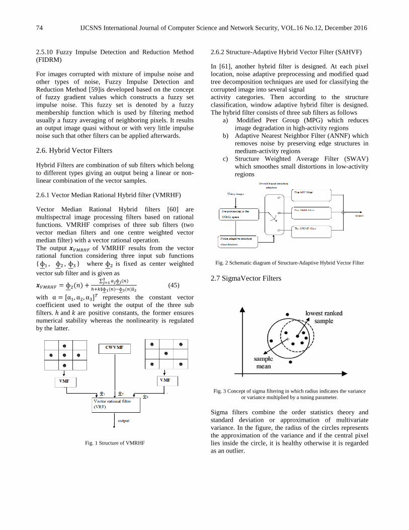
2.6.1 Vector Median Rational Hybrid filter (VMRHF)

Vector Median Rational Hybrid filters [60] are multispectral image processing filters based on rational functions. VMRHF comprises of three sub filters (two vector median filters and one centre weighted vector median filter) with a vector rational operation. The output 𝒙𝒙𝑉𝑉𝑉𝑉𝑅𝑅𝐹𝐹𝑉𝑉 of VMRHF results from the vector rational function considering three input sub functions ɸ1 , ɸ2 , ɸ3 where ɸ2 is fixed as center weighted vector sub filter and is given as

𝒙𝒙𝑉𝑉𝑉𝑉𝑅𝑅𝐹𝐹𝑉𝑉 = ɸ2(𝑚𝑚) +∑ 𝑎𝑎𝑗𝑗ɸ𝑗𝑗3𝑗𝑗=1 (𝑚𝑚)

ℎ+𝑘𝑘∥ɸ1(𝑚𝑚)−ɸ3(𝑚𝑚)∥2 (45)

with = [1,2,3]𝑅𝑅 represents the constant vector coefficient used to weight the output of the three sub filters. ℎ and 𝑘𝑘 are positive constants, the former ensures numerical stability whereas the nonlinearity is regulated by the latter.

Fig. 1 Structure of VMRHF

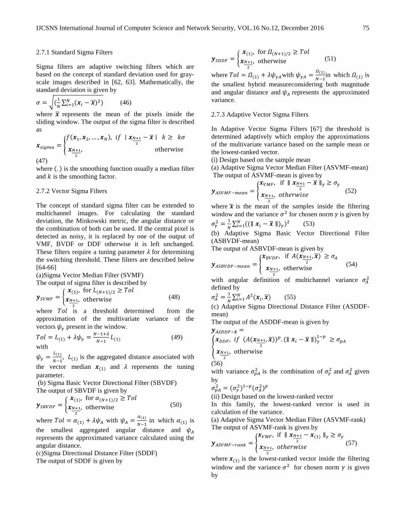
2.6.2 Structure-Adaptive Hybrid Vector Filter (SAHVF)

In [61], another hybrid filter is designed. At each pixel location, noise adaptive preprocessing and modified quad tree decomposition techniques are used for classifying the corrupted image into several signal activity categories. Then according to the structure classification, window adaptive hybrid filter is designed. The hybrid filter consists of three sub filters as follows

a) Modified Peer Group (MPG) which reduces image degradation in high-activity regions

b) Adaptive Nearest Neighbor Filter (ANNF) which removes noise by preserving edge structures in medium-activity regions

c) Structure Weighted Average Filter (SWAV) which smoothes small distortions in low-activity regions

Fig. 2 Schematic diagram of Structure-Adaptive Hybrid Vector Filter

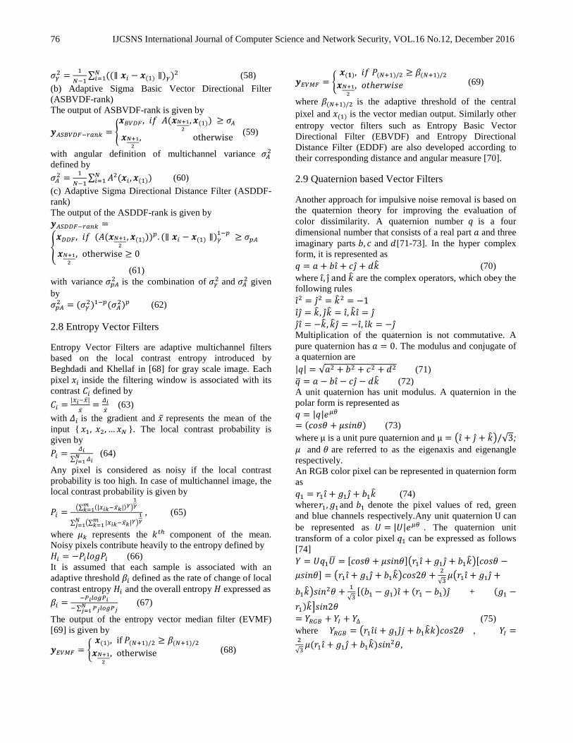
2.7 SigmaVector Filters

Fig. 3 Concept of sigma filtering in which radius indicates the variance or variance multiplied by a tuning parameter.

Sigma filters combine the order statistics theory and standard deviation or approximation of multivariate variance. In the figure, the radius of the circles represents the approximation of the variance and if the central pixel lies inside the circle, it is healthy otherwise it is regarded as an outlier.


2.7.1 Standard Sigma Filters

Sigma filters are adaptive switching filters which are based on the concept of standard deviation used for gray-scale images described in [62, 63]. Mathematically, the standard deviation is given by

𝜎𝜎 = (1𝑁𝑁∑ (𝒙𝒙𝑖𝑖 − 𝒙𝒙)2𝑁𝑁𝑖𝑖=1 ) (46)

where 𝒙𝒙 represents the mean of the pixels inside the sliding window. The output of the sigma filter is described as

𝒙𝒙𝑠𝑠𝑖𝑖𝑠𝑠𝑚𝑚𝑎𝑎 = 𝑖𝑖(𝒙𝒙1,𝒙𝒙2, … ,𝒙𝒙𝑁𝑁), 𝑖𝑖𝑖𝑖 ∣ 𝒙𝒙𝑁𝑁+1

2− 𝒙𝒙 ∣ 𝑘𝑘 ≥ 𝑘𝑘𝜎𝜎

𝒙𝒙𝑁𝑁+12

, otherwise

(47) where (. ) is the smoothing function usually a median filter and 𝑘𝑘 is the smoothing factor.

2.7.2 Vector Sigma Filters

The concept of standard sigma filter can be extended to multichannel images. For calculating the standard deviation, the Minkowski metric, the angular distance or the combination of both can be used. If the central pixel is detected as noisy, it is replaced by one of the output of VMF, BVDF or DDF otherwise it is left unchanged. These filters require a tuning parameter 𝜆𝜆 for determining the switching threshold. These filters are described below [64-66] (a)Sigma Vector Median Filter (SVMF) The output of sigma filter is described by

𝒚𝒚𝑆𝑆𝑉𝑉𝑉𝑉𝑉𝑉 = 𝒙𝒙(1), for 𝐿𝐿(𝑁𝑁+1)/2 ≥ 𝑇𝑇𝑇𝑇𝑉𝑉𝒙𝒙𝑁𝑁+1

2, otherwise (48)

where 𝑇𝑇𝑇𝑇𝑉𝑉 is a threshold determined from the approximation of the multivariate variance of the vectors 𝜓𝜓𝛾𝛾 present in the window. 𝑇𝑇𝑇𝑇𝑉𝑉 = 𝐿𝐿(1) + 𝜆𝜆𝜓𝜓𝛾𝛾 = 𝑁𝑁−1+𝜆𝜆

𝑁𝑁−1𝐿𝐿(1) (49)

with 𝜓𝜓𝛾𝛾 =

𝐶𝐶(1)

𝑁𝑁−1, 𝐿𝐿(1) is the aggregated distance associated with

the vector median 𝒙𝒙(1) and 𝜆𝜆 represents the tuning parameter. (b) Sigma Basic Vector Directional Filter (SBVDF) The output of SBVDF is given by

𝒚𝒚𝑆𝑆𝑅𝑅𝑉𝑉𝐷𝐷𝑉𝑉 = 𝒙𝒙(1), for 𝛼𝛼(𝑁𝑁+1)/2 ≥ 𝑇𝑇𝑇𝑇𝑉𝑉𝒙𝒙𝑁𝑁+1

2, otherwise (50)

where 𝑇𝑇𝑇𝑇𝑉𝑉 = 𝛼𝛼(1) + 𝜆𝜆𝜓𝜓𝐴𝐴 with 𝜓𝜓𝐴𝐴 =𝛼𝛼(1)

𝑁𝑁−1 in which 𝛼𝛼(1) is

the smallest aggregated angular distance and 𝜓𝜓𝐴𝐴 represents the approximated variance calculated using the angular distance. (c)Sigma Directional Distance Filter (SDDF) The output of SDDF is given by

𝒚𝒚𝑆𝑆𝐷𝐷𝐷𝐷𝑉𝑉 = 𝒙𝒙(1), for 𝛺𝛺(𝑁𝑁+1)/2 ≥ 𝑇𝑇𝑇𝑇𝑉𝑉𝒙𝒙𝑁𝑁+1

2, otherwise (51)

where 𝑇𝑇𝑇𝑇𝑉𝑉 = 𝛺𝛺(1) + 𝜆𝜆𝜓𝜓𝛾𝛾𝐴𝐴with 𝜓𝜓𝛾𝛾𝐴𝐴 =𝛺𝛺(1)

𝑁𝑁−1in which 𝛺𝛺(1) is

the smallest hybrid measureconsidering both magnitude and angular distance and 𝜓𝜓𝐴𝐴 represents the approximated variance.

2.7.3 Adaptive Vector Sigma Filters

In Adaptive Vector Sigma Filters [67] the threshold is determined adaptively which employ the approximations of the multivariate variance based on the sample mean or the lowest-ranked vector. (i) Design based on the sample mean (a) Adaptive Sigma Vector Median Filter (ASVMF-mean) The output of ASVMF-mean is given by

𝒚𝒚𝐴𝐴𝑆𝑆𝑉𝑉𝑉𝑉𝑉𝑉−𝑚𝑚𝑠𝑠𝑎𝑎𝑚𝑚 = 𝒙𝒙𝑉𝑉𝑉𝑉𝑉𝑉 , if ∥ 𝒙𝒙𝑁𝑁+1

2− 𝒙𝒙 ∥𝛾𝛾 ≥ 𝜎𝜎𝛾𝛾

𝒙𝒙𝑁𝑁+12

, 𝑇𝑇𝑜𝑜ℎ𝑒𝑒𝑟𝑟𝑤𝑤𝑖𝑖𝑠𝑠𝑒𝑒 (52)

where 𝒙𝒙 is the mean of the samples inside the filtering window and the variance 𝜎𝜎2 for chosen norm 𝛾𝛾 is given by 𝜎𝜎𝛾𝛾2 = 1

𝑁𝑁∑ ((∥ 𝒙𝒙𝑖𝑖 − 𝒙𝒙 ∥)𝛾𝛾)2𝑁𝑁𝑖𝑖=1 (53)

(b) Adaptive Sigma Basic Vector Directional Filter (ASBVDF-mean) The output of ASBVDF-mean is given by

𝒚𝒚𝐴𝐴𝑆𝑆𝑅𝑅𝑉𝑉𝐷𝐷𝑉𝑉−𝑚𝑚𝑠𝑠𝑎𝑎𝑚𝑚 = 𝒙𝒙𝑅𝑅𝑉𝑉𝐷𝐷𝑉𝑉 , if 𝐴𝐴(𝒙𝒙𝑁𝑁+1

2,𝒙𝒙) ≥ 𝜎𝜎𝐴𝐴

𝒙𝒙𝑁𝑁+12

, otherwise (54)

with angular definition of multichannel variance 𝜎𝜎𝐴𝐴2 defined by 𝜎𝜎𝐴𝐴2 = 1

𝑁𝑁∑ 𝐴𝐴2(𝒙𝒙𝑖𝑖 ,𝒙𝒙)𝑁𝑁𝑖𝑖=1 (55)

(c) Adaptive Sigma Directional Distance Filter (ASDDF-mean) The output of the ASDDF-mean is given by 𝒚𝒚𝐴𝐴𝑆𝑆𝐷𝐷𝐷𝐷𝑉𝑉−𝒙𝒙 =

𝒙𝒙𝐷𝐷𝐷𝐷𝑉𝑉, 𝑖𝑖𝑖𝑖 (𝐴𝐴(𝒙𝒙𝑁𝑁+1

2,𝒙𝒙))𝑝𝑝. (∥ 𝒙𝒙𝑖𝑖 − 𝒙𝒙 ∥)𝛾𝛾

1−𝑝𝑝 ≥ 𝜎𝜎𝑝𝑝𝐴𝐴𝒙𝒙𝑁𝑁+1

2, otherwise

(56) with variance 𝜎𝜎𝑝𝑝𝐴𝐴2 is the combination of 𝜎𝜎𝛾𝛾2 and 𝜎𝜎𝐴𝐴2 given by 𝜎𝜎𝑝𝑝𝐴𝐴2 = (𝜎𝜎𝛾𝛾2)1−𝑝𝑝(𝜎𝜎𝐴𝐴2)𝑝𝑝 (ii) Design based on the lowest-ranked vector In this family, the lowest-ranked vector is used in calculation of the variance. (a) Adaptive Sigma Vector Median Filter (ASVMF-rank) The output of ASVMF-rank is given by

𝒚𝒚𝐴𝐴𝑆𝑆𝑉𝑉𝑉𝑉𝑉𝑉−𝑟𝑟𝑎𝑎𝑚𝑚𝑘𝑘 = 𝒙𝒙𝑉𝑉𝑉𝑉𝑉𝑉 , if ∥ 𝒙𝒙𝑁𝑁+1

2− 𝒙𝒙(1) ∥𝛾𝛾 ≥ 𝜎𝜎𝛾𝛾

𝒙𝒙𝑁𝑁+12


where 𝒙𝒙(1) is the lowest-ranked vector inside the filtering window and the variance 𝜎𝜎2 for chosen norm 𝛾𝛾 is given by


𝜎𝜎𝛾𝛾2 = 1𝑁𝑁−1

∑ ((∥ 𝒙𝒙𝑖𝑖 − 𝒙𝒙(1) ∥)𝛾𝛾)2𝑁𝑁𝑖𝑖=1 (58)

(b) Adaptive Sigma Basic Vector Directional Filter (ASBVDF-rank) The output of ASBVDF-rank is given by

𝒚𝒚𝐴𝐴𝑆𝑆𝑅𝑅𝑉𝑉𝐷𝐷𝑉𝑉−𝑟𝑟𝑎𝑎𝑚𝑚𝑘𝑘 = 𝒙𝒙𝑅𝑅𝑉𝑉𝐷𝐷𝑉𝑉 , 𝑖𝑖𝑖𝑖 𝐴𝐴(𝒙𝒙𝑁𝑁+1

2,𝒙𝒙(1)) ≥ 𝜎𝜎𝐴𝐴

𝒙𝒙𝑁𝑁+12

, otherwise (59)

with angular definition of multichannel variance 𝜎𝜎𝐴𝐴2 defined by 𝜎𝜎𝐴𝐴2 = 1

𝑁𝑁−1∑ 𝐴𝐴2(𝒙𝒙𝑖𝑖 ,𝒙𝒙(1))𝑁𝑁𝑖𝑖=1 (60)

(c) Adaptive Sigma Directional Distance Filter (ASDDF-rank) The output of the ASDDF-rank is given by 𝒚𝒚𝐴𝐴𝑆𝑆𝐷𝐷𝐷𝐷𝑉𝑉−𝑟𝑟𝑎𝑎𝑚𝑚𝑘𝑘 =

𝒙𝒙𝐷𝐷𝐷𝐷𝑉𝑉, 𝑖𝑖𝑖𝑖 (𝐴𝐴(𝒙𝒙𝑁𝑁+1

2,𝒙𝒙(1)))𝑝𝑝. (∥ 𝒙𝒙𝑖𝑖 − 𝒙𝒙(1) ∥)𝛾𝛾

1−𝑝𝑝 ≥ 𝜎𝜎𝑝𝑝𝐴𝐴𝒙𝒙𝑁𝑁+1

2, otherwise ≥ 0

(61) with variance 𝜎𝜎𝑝𝑝𝐴𝐴2 is the combination of 𝜎𝜎𝛾𝛾2 and 𝜎𝜎𝐴𝐴2 given by 𝜎𝜎𝑝𝑝𝐴𝐴2 = (𝜎𝜎𝛾𝛾2)1−𝑝𝑝(𝜎𝜎𝐴𝐴2)𝑝𝑝 (62)

2.8 Entropy Vector Filters

Entropy Vector Filters are adaptive multichannel filters based on the local contrast entropy introduced by Beghdadi and Khellaf in [68] for gray scale image. Each pixel 𝑥𝑥𝑖𝑖 inside the filtering window is associated with its contrast 𝐶𝐶𝑖𝑖 defined by 𝐶𝐶𝑖𝑖 = |𝑥𝑥𝑖𝑖−𝑥|

𝑥= 𝛥𝛥𝑖𝑖

𝑥 (63)

with 𝛥𝛥𝑖𝑖 is the gradient and 𝑥 represents the mean of the input 𝑥𝑥1, 𝑥𝑥2, … 𝑥𝑥𝑁𝑁 . The local contrast probability is given by 𝑃𝑃𝑖𝑖 = 𝛥𝛥𝑖𝑖

∑ 𝛥𝛥𝑖𝑖𝑁𝑁𝑗𝑗=1

(64)

Any pixel is considered as noisy if the local contrast probability is too high. In case of multichannel image, the local contrast probability is given by

𝑃𝑃𝑖𝑖 = ∑ (|𝑥𝑥𝑖𝑖𝑖𝑖−𝑥𝑖𝑖|)𝛾𝛾𝑚𝑚𝑖𝑖=1

1𝛾𝛾

∑ ∑ |𝑥𝑥𝑖𝑖𝑖𝑖−𝑥𝑖𝑖|𝛾𝛾𝑚𝑚𝑖𝑖=1

1𝛾𝛾𝑁𝑁

𝑗𝑗=1

, (65)

where 𝜇𝜇𝑘𝑘 represents the 𝑘𝑘𝑡𝑡ℎ component of the mean. Noisy pixels contribute heavily to the entropy defined by 𝐻𝐻𝑖𝑖 = −𝑃𝑃𝑖𝑖𝑉𝑉𝑇𝑇𝑎𝑎𝑃𝑃𝑖𝑖 (66) It is assumed that each sample is associated with an adaptive threshold 𝛽𝛽𝑖𝑖 defined as the rate of change of local contrast entropy 𝐻𝐻𝑖𝑖 and the overall entropy 𝐻𝐻 expressed as 𝛽𝛽𝑖𝑖 = −𝑃𝑃𝑖𝑖𝑙𝑙𝑜𝑜𝑠𝑠𝑃𝑃𝑖𝑖

−∑ 𝑃𝑃𝑗𝑗𝑙𝑙𝑜𝑜𝑠𝑠𝑃𝑃𝑗𝑗𝑁𝑁𝑗𝑗=1

(67)

The output of the entropy vector median filter (EVMF) [69] is given by

𝒚𝒚𝐸𝐸𝑉𝑉𝑉𝑉𝑉𝑉 = 𝒙𝒙(1), if 𝑃𝑃(𝑁𝑁+1)/2 ≥ 𝛽𝛽(𝑁𝑁+1)/2

𝒙𝒙𝑁𝑁+12

, otherwise (68)

𝒚𝒚𝐸𝐸𝑉𝑉𝑉𝑉𝑉𝑉 = 𝒙𝒙(𝟏𝟏), 𝑖𝑖𝑖𝑖 𝑃𝑃(𝑁𝑁+1)/2 ≥ 𝛽𝛽(𝑁𝑁+1)/2

𝒙𝒙𝑁𝑁+12


where 𝛽𝛽(𝑁𝑁+1)/2 is the adaptive threshold of the central pixel and 𝑥𝑥(1) is the vector median output. Similarly other entropy vector filters such as Entropy Basic Vector Directional Filter (EBVDF) and Entropy Directional Distance Filter (EDDF) are also developed according to their corresponding distance and angular measure [70].

2.9 Quaternion based Vector Filters

Another approach for impulsive noise removal is based on the quaternion theory for improving the evaluation of color dissimilarity. A quaternion number 𝑞𝑞 is a four dimensional number that consists of a real part 𝑎𝑎 and three imaginary parts 𝑏𝑏, 𝑐𝑐 and 𝑑𝑑[71-73]. In the hyper complex form, it is represented as 𝑞𝑞 = 𝑎𝑎 + 𝑏𝑏𝚤𝚤 + 𝑐𝑐𝚥𝚥 + 𝑑𝑑𝑘𝑘 (70) where 𝚤𝚤, ȷ and 𝑘𝑘 are the complex operators, which obey the following rules 𝚤𝚤2 = 𝚥𝚥2 = 𝑘𝑘2 = −1 𝚤𝚤𝚥𝚥 = 𝑘𝑘 , 𝚥𝚥𝑘𝑘 = 𝚤𝚤, 𝑘𝑘𝚤𝚤 = 𝚥𝚥 𝚥𝚥𝚤𝚤 = −𝑘𝑘 , 𝑘𝑘𝚥𝚥 = −𝚤𝚤, 𝚤𝚤𝑘 = −𝚥𝚥 Multiplication of the quaternion is not commutative. A pure quaternion has 𝑎𝑎 = 0. The modulus and conjugate of a quaternion are |𝑞𝑞| = √𝑎𝑎2 + 𝑏𝑏2 + 𝑐𝑐2 + 𝑑𝑑2 (71) 𝑞𝑞 = 𝑎𝑎 − 𝑏𝑏𝚤𝚤 − 𝑐𝑐𝚥𝚥 − 𝑑𝑑𝑘𝑘 (72) A unit quaternion has unit modulus. A quaternion in the polar form is represented as 𝑞𝑞 = |𝑞𝑞|𝑒𝑒𝜇𝜇𝜇𝜇 = (𝑐𝑐𝑇𝑇𝑠𝑠𝜃𝜃 + 𝜇𝜇𝑠𝑠𝑖𝑖𝑚𝑚𝜃𝜃) (73) where µ is a unit pure quaternion and µ = 𝚤𝚤 + 𝚥𝚥 + 𝑘𝑘/√3; 𝜇𝜇 and 𝜃𝜃 are referred to as the eigenaxis and eigenangle respectively. An RGB color pixel can be represented in quaternion form as 𝑞𝑞1 = 𝑟𝑟1𝚤𝚤 + 𝑎𝑎1𝚥𝚥 + 𝑏𝑏1𝑘𝑘 (74) where𝑟𝑟1,𝑎𝑎1and 𝑏𝑏1 denote the pixel values of red, green and blue channels respectively.Any unit quaternion U can be represented as 𝑈𝑈 = |𝑈𝑈|𝑒𝑒𝜇𝜇𝜇𝜇 . The quaternion unit transform of a color pixel 𝑞𝑞1 can be expressed as follows [74] 𝑌𝑌 = 𝑈𝑈𝑞𝑞1𝑈𝑈 = [𝑐𝑐𝑇𝑇𝑠𝑠𝜃𝜃 + 𝜇𝜇𝑠𝑠𝑖𝑖𝑚𝑚𝜃𝜃]𝑟𝑟1𝚤𝚤 + 𝑎𝑎1𝚥𝚥 + 𝑏𝑏1𝑘𝑘[𝑐𝑐𝑇𝑇𝑠𝑠𝜃𝜃 −𝜇𝜇𝑠𝑠𝑖𝑖𝑚𝑚𝜃𝜃] = 𝑟𝑟1𝚤𝚤 + 𝑎𝑎1𝚥𝚥 + 𝑏𝑏1𝑘𝑘𝑐𝑐𝑇𝑇𝑠𝑠2𝜃𝜃 + 2

√3𝜇𝜇𝑟𝑟1𝚤𝚤 + 𝑎𝑎1𝚥𝚥 +

𝑏𝑏1𝑘𝑘𝑠𝑠𝑖𝑖𝑚𝑚2𝜃𝜃 + 1√3

[(𝑏𝑏1 − 𝑎𝑎1)𝚤𝚤 + (𝑟𝑟1 − 𝑏𝑏1)𝚥𝚥 + (𝑎𝑎1 −𝑟𝑟1)𝑘𝑘𝑠𝑠𝑖𝑖𝑚𝑚2𝜃𝜃 = 𝑌𝑌𝑅𝑅𝐺𝐺𝑅𝑅 + 𝑌𝑌𝐼𝐼 + 𝑌𝑌∆ (75) where 𝑌𝑌𝑅𝑅𝐺𝐺𝑅𝑅 = 𝑟𝑟1𝚤𝚤𝑖𝑖 + 𝑎𝑎1𝚥𝚥𝑗𝑗 + 𝑏𝑏1𝑘𝑘𝑘𝑘𝑐𝑐𝑇𝑇𝑠𝑠2𝜃𝜃 , 𝑌𝑌𝐼𝐼 =2√3𝜇𝜇(𝑟𝑟1𝚤𝚤 + 𝑎𝑎1𝚥𝚥 + 𝑏𝑏1𝑘𝑘)𝑠𝑠𝑖𝑖𝑚𝑚2𝜃𝜃,


𝑌𝑌∆ = 1√3

[(𝑏𝑏1 − 𝑎𝑎1)𝚤𝚤 + (𝑟𝑟1 − 𝑏𝑏1)𝚥𝚥 + (g1 − r1)k𝑠𝑠𝑖𝑖𝑚𝑚2𝜃𝜃 ; 𝑌𝑌 𝐼𝐼 represents the intensity of the color image; 𝑌𝑌∆ is the projection of the tristimuli in Maxwell triangle rotated 900, and it represents the chromaticity [3]. When𝜃𝜃 = 𝜋𝜋

4, 𝑇𝑇 =

𝑈𝑈|𝜇𝜇=𝜋𝜋4= 1 √2⁄ + 1 √6⁄ 𝚤𝚤 + 𝚥𝚥 + 𝑘𝑘and𝑌𝑌𝑅𝑅𝐺𝐺𝑅𝑅 = 0, 𝑌𝑌𝐼𝐼 =

(1 3⁄ )(𝑟𝑟1 + 𝑎𝑎1 + 𝑏𝑏1)𝚤𝚤 + 𝚥𝚥 + 𝑘𝑘 and 𝑌𝑌∆ = 1 √3⁄ [ (𝑏𝑏1 −𝑎𝑎1)𝚤𝚤 + (𝑟𝑟1 − 𝑏𝑏1)𝚥𝚥 + (𝑎𝑎1 − 𝑟𝑟1)𝑘𝑘] .Similarly, 𝑌𝑌 can be defined as follows 𝑌𝑌 = 𝑇𝑇𝑞𝑞1𝑇𝑇 = 1

3(𝑟𝑟1 + 𝑎𝑎1 + 𝑏𝑏1)𝚤𝚤 + 𝚥𝚥 + 𝑘𝑘 − 1

√3[(𝑏𝑏1 −

𝑎𝑎1)𝚤𝚤 + (𝑟𝑟1 − 𝑏𝑏1)𝚥𝚥 + (𝑎𝑎1 − 𝑟𝑟1)𝑘𝑘] = 𝑌𝑌𝐼𝐼 − 𝑌𝑌∆ (76) 𝑌𝑌 𝐼𝐼 and 𝑌𝑌∆ can be expressed as 𝑌𝑌𝐼𝐼 = 1

2(𝑇𝑇𝑞𝑞1𝑇𝑇 +

𝑇𝑇𝑞𝑞1𝑇𝑇)and𝑌𝑌∆ = 12

(𝑇𝑇𝑞𝑞1𝑇𝑇 − 𝑇𝑇𝑞𝑞1𝑇𝑇). The color pixel difference between two pixels 𝑞𝑞𝑖𝑖 and 𝑞𝑞𝑗𝑗 can be written as the sum of the intensity and chromaticity differences as follows: 𝑑𝑑𝑞𝑞𝑖𝑖 , 𝑞𝑞𝑗𝑗 = 𝑑𝑑𝐼𝐼𝑞𝑞𝑖𝑖 , 𝑞𝑞𝑗𝑗 + 𝑑𝑑∆𝑞𝑞𝑖𝑖 , 𝑞𝑞𝑗𝑗 (76) where 𝑑𝑑𝐼𝐼𝑞𝑞𝑖𝑖 , 𝑞𝑞𝑗𝑗 = (1 2⁄ )|(𝑇𝑇𝑞𝑞𝑖𝑖𝑇𝑇 + 𝑇𝑇𝑞𝑞𝑖𝑖𝑇𝑇) − (𝑇𝑇𝑞𝑞𝑗𝑗𝑇𝑇 +𝑇𝑇𝑞𝑞𝑗𝑗𝑇𝑇)| is the color intensity difference and 𝑑𝑑∆𝑞𝑞𝑖𝑖 , 𝑞𝑞𝑗𝑗 = (1 2⁄ )|(𝑇𝑇𝑞𝑞𝑖𝑖𝑇𝑇 − 𝑇𝑇𝑞𝑞𝑖𝑖𝑇𝑇) − (𝑇𝑇𝑞𝑞𝑗𝑗𝑇𝑇 −𝑇𝑇𝑞𝑞𝑗𝑗𝑇𝑇)|is the color chromaticity difference.The intensity difference and chromaticity difference approach zero when 𝑞𝑞𝑖𝑖 is very similar to 𝑞𝑞𝑗𝑗. In [75-76] a switching VMF based on quaternion impulse detector is proposed using 5× 5 window. The quaternion color difference between pixels along the four directional operators at0°, 45°, 90°and135° are computed. An average color difference 𝑉𝑉𝑎𝑎𝑉𝑉ℎbetween the central pixel and other pixel values in the directionℎ = (1, 2, 3,4) for respective degrees are computed as follows: 𝑉𝑉𝑎𝑎𝑉𝑉ℎ = 1

4∑ ∣ 𝑑𝑑𝒙𝒙𝑖𝑖 ,𝒙𝒙𝑗𝑗 ∣4𝑗𝑗=1 (77)

𝑉𝑉𝑎𝑎𝑉𝑉 = min (𝑉𝑉𝑎𝑎𝑉𝑉1,𝑉𝑉𝑎𝑎𝑉𝑉2,𝑉𝑉𝑎𝑎𝑉𝑉3,𝑉𝑉𝑎𝑎𝑉𝑉4) The above two equations are used for impulse detection. If the central pixel is an impulse, its 𝑉𝑉𝑎𝑎𝑉𝑉 value will be large otherwise it is small. Hence the output of the filter is given by

𝒙𝒙𝑄𝑄𝑉𝑉𝑉𝑉𝑉𝑉 = 𝑄𝑄(𝑉𝑉𝑉𝑉𝑉𝑉), if 𝑉𝑉𝑎𝑎𝑉𝑉 ≥ 𝑇𝑇𝒙𝒙(𝑁𝑁+1)/2, otherwise (78)

where 𝑄𝑄(𝑉𝑉𝑉𝑉𝑉𝑉)represents the VMF calculated in Quaternion form and T being a pre-specified threshold. In [77] another Quaternion Switching Vector Median Filter (QSVMF) is developed based on both the intensity and chromaticity differences described above. A modification of QSVMF is designed in [78]. It is different from other related works in the impulse detection which utilizes the pixels along only a direction with maximum number of similar pixels while other utilize the color differences between the central pixel and its neighboring pixels in the four-edge direction. A two-stage filter using both the Quaternion based Switching filter and a local mean filter is designed in [79]

for removing mixture noise. In [80] a new two-stage filter is proposed which incorporates the peer group concept along with the quaternion based distance measure for impulse detection. The probably noisy pixels are replaced by Weighted Vector Median Filter in the second stage. The concept of quaternion is extended in video sequences for removal of random-valued impulse noise in [81]. The luminance and chromaticity difference are represented in quaternion form which are combined together for measuring color difference between color samples. Based on this color difference, the color vectors along the horizontal, vertical and diagonal directions in current frame and adjacent frames on motion trajectory are utilize for the detection of presence of impulse. For noisy pixels, a 3-D weighted vector median operation is carried out while the other pixels are left intact. Another filter for removal of random-valued impulse noise from video sequences is also designed in [82].

2.10 Morphology based filters

Morphological filters (MF) are designed by parallel or sequential combination of the basic fundamental morphological operations such as erosion, dilation, opening and closing [83-85]. The common structures of MF are defined as OC Filter → Opening followed by Closing CO Filter → Closing followed by Opening (79) Erosion distributes the local minima while dilation distributes the local maxima within the sliding window defined by the structuring element which resembles a min/max filtering action for suppression of impulse noise. In [86], an extension of MF to multichannel images on learning-based morphological color operations is developed. The color pixel ordering scheme is learned in accordance to pre-estimation of healthy and corrupted pixels where the corrupted samples are ordered either as maximum in erosion or minimum in dilation. The SVM is used as the classification technique of such learning-based multichannel MF in the RGB color domain. After each morphological operation, the image reconstruction step is carried out for restoring the original features. Extension of mathematical morphology to multivariable data such as multichannel image is performed in [87-89]. In order to develop multivariate morphological operators, various complex mathematical tools such as machine learning [90], principal component analysis [91], hyper complex [92], rand projection depth function [93], group-invariant frames [94], and probabilistic extrema estimation [95] are used. Based on the self-duality property of morphological operator, a multivariate self-dual morphological operator is developed in [96] which is applicable for noise removal and segmentation purposes. A pair of symmetric vector


ordering is introduced in order to develop multivariate dual morphological operators. Quantile filters and a group of morphological gradient filters are proposed in [97]. Their properties and links with dilation and erosion operators are also investigated. Another quantile filter is also designed in [98]. In [99], a new hybrid filter based on mathematical morphology and trimmed standard median filter is developed. For impulse detection, mathematical morphology such as erosion and dilation are utilized. Erosion refers to the computation of local minima while dilation estimates the local maxima of the neighboring pixels. The existence of an inverse relationship between erosion and dilation is used for detection for salt & pepper noise.

2.11 Wavelet-Transform based Filters

Many nonlinear filtering techniques are designed based on wavelet transform. Haci Tasmaz et al., [100] proposes a satellite image enhancement system comprising of image denoising and illumination enhancement technique. It is based on dual tree complex wavelet transform (DT-CWT). Based on the combined effect of Haar wavelet transform and median filter, a denoising technique is also proposed [101]. In [102], another denoising algorithm based on combined effect of the bi-orthogonal wavelet transform and median filter is designed which removes noise effectively. In [103], a wavelet based denoising technique for suppression of noise in Magnetic Resonance images (MRI) is proposed. Shalini and Godwin in [104] present a comparative analysis of denoising algorithms based on different wavelet transform such as Bior, Surelet, Haar and Curvelet.

2.12 Miscellaneous Filters

Miscellaneous Filters consist of those filters which cannot be included into any of the filter families described above although some filters may have common properties.

2.12.1 Selective Vector Median Filter

In [105] Selective Vector Median Filter is introduced which has two steps: noise detection and noise removal. For every pixel in the window aggregated sum of distance between other pixels is computed 𝑆𝑆𝑖𝑖 = ∑ ∥ 𝒙𝒙𝑖𝑖 − 𝒙𝒙𝑗𝑗 ∥, 𝑖𝑖 = 1, …𝑁𝑁𝑁𝑁

𝑗𝑗=1 (80) Then the mean 𝑆𝑆 value for that neighborhood is calculated as follows 𝑆𝑆 = 1

𝑁𝑁∑ 𝑆𝑆𝑗𝑗𝑁𝑁𝑗𝑗=1 (81)

The pixels which have 𝑆𝑆 value higher than 𝑘𝑘𝑆𝑆 in the neighborhood are flagged as outliers. 𝑘𝑘 represents a constant used to increase or decrease the sensitivity of the threshold. If the central pixel is an outlier, then the

remaining pixels which are not flagged as outliers are used for calculating the Vector median and the noisy pixel is replaced by the corresponding vector median.

2.12.2 Similarity based Impulsive Noise Removal Filter

In [106] a filter based on similarities between the pixels in a predefined window is developed. If 𝒙𝒙𝑖𝑖 , … ,𝒙𝒙𝑁𝑁 denote the pixels in a filtering window, then a convex similarity function is used to find the similarity between pixels. For the central pixel and its neighboring pixels, the cumulated sum of similarities 𝑀𝑀 are computed as follows: 𝑀𝑀1 = ∑ µ(𝒙𝒙1,𝒙𝒙𝑗𝑗)𝑁𝑁

𝑗𝑗=2 , 𝑀𝑀𝑘𝑘 = ∑ µ(𝒙𝒙𝑘𝑘,𝒙𝒙𝑗𝑗)𝑁𝑁

𝑗𝑗=2,𝑗𝑗≠𝑘𝑘 (82) 𝒙𝒙1 is the central pixel and µ(𝒙𝒙𝑖𝑖,𝒙𝒙𝑗𝑗)is a convex similarity function. The central pixel is detected as noisy if 𝑀𝑀1 <𝑀𝑀𝑘𝑘, 𝑘𝑘 = 2, … ,𝑁𝑁and is replaced by that 𝒙𝒙𝑘𝑘 for which 𝑘𝑘 =𝑎𝑎𝑟𝑟𝑎𝑎𝑚𝑚𝑎𝑎𝑥𝑥𝑀𝑀𝑖𝑖, 𝑘𝑘 = 2, … ,𝑁𝑁.This filter is faster than VMF. A similar filter based on this idea is also developed in [107].

2.12.3 Filters based on Digital Path Approach

In [108] noise filtering approach based on the connections between image samples using the digital geodesic path is developed instead of using a fixed window. In this filter the image pixels are grouped togetherthrough the fuzzy membership function defined over vectorial inputs by forming digital paths revealing the underlying structure dynamics of the image. It shows better performance in suppressing impulsive, Gaussian as well as mixed-type noise.

2.12.4 Filters based on Long Range Correlation

Traditional method of noise filtering utilizes information based on local window centered around the corrupted pixel. In [109] a new class of filter based on information on both the local window and also some remote regions in the image is developed. This is due to the fact that there exists a long range correlation within natural images and also the human visual system can use such correlations to interpret and restore image information [110]. This filter comprises of two steps: impulse detection and noise cancellation. In the impulse detection stage any impulse detector as described in [111] and [112] can be used for identifying the corrupted pixel in the local window. If the central pixel is corrupted, then a remote window centered around the impulse pixel is defined in the search range which is larger than the local window. All the pixels in the remote window will compete for the perfect match with the local window based on the mean square error of uncorrupted pixels in local and remote window. Finally, the corrupted pixel is replaced by the central pixel of the remote window with minimum mean squared error.


Fig. 4 Demonstration of the general approach

2.12.5 Vector Rational Filters (VRF)

Vector rational filters are extension of rational filters. In [113], two algorithms are proposed 𝑉𝑉𝑉𝑉𝑉𝑉𝐶𝐶 and 𝑉𝑉𝑉𝑉𝑉𝑉𝑑𝑑 based on 𝐿𝐿𝑝𝑝 -norm and directional processing using two decimation schemes such as rectangular and quincunx decimation for down-sampling. Merits of these filters are better edge-preserving properties and absence of artifacts.

2.12.6 Robust Local Similarity Filters (RLSF)

A new algorithm for suppression of mixed Gaussian and impulsive noise based on concept of Rank ordered Absolute Difference (ROAD) [114] is proposed in [115]. Noise is detected by computing ROAD between samples of the processing block and a small window which is centered at block’s central pixel. Main contribution is that the similarity measure is not affected by outliers due to impulses and the averaging operation reduces the Gaussian noise. The output of this filter is given as

𝒙𝒙𝑅𝑅𝐶𝐶𝑆𝑆𝑉𝑉 =∑ 𝑤𝑤𝑗𝑗.𝒙𝒙𝑗𝑗𝑁𝑁𝑗𝑗=1∑ 𝑤𝑤𝑗𝑗𝑁𝑁𝑗𝑗=1

(83)

with 𝑤𝑤𝑗𝑗 = Ҡ1𝛼𝛼∑ 𝑑𝑑𝑗𝑗(𝑘𝑘)𝛼𝛼𝑘𝑘=1 (84)

where Ҡ represents the kernel function (Gaussian) and 𝑑𝑑𝑗𝑗(𝑘𝑘) denotes the 𝑘𝑘𝑡𝑡ℎ smallest Euclidean distance between pixel 𝑥𝑥𝑗𝑗 of the processing block and pixels of 𝑊𝑊 of the small window. 𝛼𝛼 is the number of close neighbors used in calculation of ROAD.

Fig. 5 Calculation of similarity measure between pixel in the processing block (Green Square) and small window (red square) by ROAD.

2.12.7 Vector Marginal Median Filters (VMMF)

In [3] a vector filter named Vector Marginal Median Filter (VMMF) based on the median operation is presented. It calculates the median value of each channel separately and the central pixel is replaced by the median value of the respective channel. The output of VMMF is given below 𝒙𝒙𝑉𝑉𝑉𝑉𝑉𝑉𝑉𝑉 =((𝑚𝑚𝑒𝑒𝑑𝑑(𝑥𝑥1𝑅𝑅 , … 𝑥𝑥𝑁𝑁𝑅𝑅)), 𝑚𝑚𝑒𝑒𝑑𝑑(𝑥𝑥1𝐺𝐺 , … 𝑥𝑥𝑁𝑁𝐺𝐺), (𝑚𝑚𝑒𝑒𝑑𝑑(𝑥𝑥1𝑅𝑅, … 𝑥𝑥𝑁𝑁𝑅𝑅))) (85) where 𝑉𝑉,𝐺𝐺 and 𝐵𝐵 are the red, green and blue channel of the pixels in the window. Its noise reduction capability is highest but since it does not consider the correlation among the vector channel, it leads to color artifacts.

2.12.8 Vector Signal-Dependent Rank Order Mean Filters

Multichannel extension of the grayscale Signal Dependent Rank Order Mean (SDROM) filter [116] is the Vector signal-dependent rank order mean (VSDROM) filter [117]. For noise detection, first the vector pixels in the window are sorted according to their aggregated distance to all other samples. The distance between the four lowest-ranked vectors and the central pixel are compared against respective increasing thresholds. The central pixel is regarded as noisy if any of these distances is greater than their threshold and replaced by the VMF.

2.12.9 Decision based Couple Window Median Filters (DBCWMF)

They use an increasing window size in order to maximize the probability of finding noise-free pixels [118]. The steps of DBCWMF is given below 1. Define a 2-D local window 𝑊𝑊𝑚𝑚 of dimension (2𝑚𝑚 +1) × (2𝑚𝑚 + 1) (initialize algorithm by choosing 𝑚𝑚 = 1). 2. Identify salt & pepper noise by checking if the central pixel 𝒙𝒙𝑁𝑁+1

2 is either 0 or 255. If 0< 𝒙𝒙𝑁𝑁+1

2< 255 it is left

intact.


3. If 𝒙𝒙𝑁𝑁+12

is noisy, then trim all 0’s and 255’s present in

the 𝑊𝑊𝑚𝑚 and follow the two cases Case 1. If the number of non-noisy pixels is non-zero, then replace the central pixel by the median value calculated from the remaining uncorrupted pixels. Case 2. If the number of non-noisy pixels is zero, then update the window size by increasing 𝑚𝑚 = 𝑚𝑚 + 1, (𝑚𝑚 < 5) and goto Step 1. 4. If the number of non-noisy pixels in 𝑊𝑊4 is zero, then replace the value of central pixel by mean of 𝑊𝑊1. 5. Repeat Steps 1 to 4 until all the pixels are processed.

2.12.10 Improved Bilateral Filter for reducing mixed noise

A Bilateral Filter (BF) [119] is a combination of two low-pass Gaussian filters operating in spatial and color (range) domain for reducing both impulse and additive noise while preserving edge structures. The spatial low-pass filter gives larger weights to those samples closer to the central pixel while the range low pass filter assigns larger weights to those pixels having similar color distributions with the central pixel. Here the filter’s output is mainly dependent on the central pixel and neighboring pixels close in both spatial and range domain with the central pixel.An improvement in the traditional Bilateral Filter (BF) is designed in [120] in which a new weighting function to the bilateral filtering mechanism is introduced. For an impulse, the vector median (as opposed to the traditional BF which always uses the central pixel) is considered as base for bilateral filtering operation for replacement of the central pixel otherwise the normal bilateral filtering action is continued.

3. Impulse Noise Model

In the real life, the form of impulse noise varies. For example, the value of impulse noise caused by malfunction of sensor is expected to be fixed-valued impulse noise, while the value of impulse caused by electronic interference is random-valued impulse noise [77]. Impulse noise can be divided into two types: Correlated impulse noise and Uncorrelated impulse noise. The impulse noise model proposed by Viero et al [10] is correlated type impulse noise and it has the following form

𝒒𝒒′ =

⎩⎪⎨

⎪⎧

𝑞𝑞1 𝑞𝑞2 𝑞𝑞3with probability 1 − 𝑝𝑝𝑚𝑚1, 𝑞𝑞2, 𝑞𝑞3with probability 𝑝𝑝1𝑝𝑝𝑞𝑞1, 𝑚𝑚2, 𝑞𝑞3with probability 𝑝𝑝2𝑝𝑝𝑞𝑞1, 𝑞𝑞2, 𝑚𝑚3with probability 𝑝𝑝3𝑝𝑝𝑚𝑚1, 𝑚𝑚2, 𝑚𝑚3with probability 𝑝𝑝𝑎𝑎𝑝𝑝

(86)

where 𝒒𝒒 = (𝑞𝑞1, 𝑞𝑞2, 𝑞𝑞3) is the original uncontaminated vector pixel, 𝒒𝒒′ may be either contaminated or

uncontaminated, 𝑚𝑚𝑘𝑘(𝑘𝑘 = 1,2,3) equals 0 or 255 with equal probability for fixed-valued impulse noise, or takes any value in the range [0,255] for random-valued impulse noise; 𝑝𝑝 is the sample corruption probability; 𝑝𝑝1, 𝑝𝑝2and 𝑝𝑝3 are the channel corruption probabilities and 𝑝𝑝𝑎𝑎 = 1 −𝑝𝑝1 − 𝑝𝑝2 − 𝑝𝑝3. The uncorrelated impulse noise has the following form [46]

𝑞𝑞𝑘𝑘′ = 𝑚𝑚𝑘𝑘 with probability 𝑝𝑝𝑞𝑞𝑘𝑘 with probability 1 − 𝑝𝑝 (87)

where 𝑘𝑘 = 1,2,3 denotes the three channels in RGB color space; 𝑝𝑝 is the channel corruption probability; 𝑞𝑞𝑘𝑘 and 𝑚𝑚𝑘𝑘 denote the original component and contaminated component respectively. 𝑚𝑚𝑘𝑘 can take either 0 or 255 for fixed-valued impulse noise and can take any discrete value in [0,255] for random-valued impulse noise.

4. Performance Measurement of Filters

The performance of filter is evaluated by the following parameters

(a) Mean Absolute Error (MAE)

𝑀𝑀𝐴𝐴𝑀𝑀 = 1𝑉𝑉1×𝑁𝑁1

∑ ∑ |𝑞𝑞(𝑖𝑖, 𝑗𝑗) − 𝑖𝑖(𝑖𝑖, 𝑗𝑗)|𝑁𝑁1𝑗𝑗=1

𝑉𝑉1𝑖𝑖=1 (88)

where 𝑀𝑀1 × 𝑁𝑁1 is the size of the image; 𝑞𝑞(𝑖𝑖, 𝑗𝑗) and 𝑖𝑖(𝑖𝑖, 𝑗𝑗) are the original and filtered pixel values at (𝑖𝑖, 𝑗𝑗) location. (b) Mean Squared Error (MSE) 𝑀𝑀𝑆𝑆𝑀𝑀 = 1

𝑉𝑉1×𝑁𝑁1∑ ∑ (𝑞𝑞(𝑖𝑖, 𝑗𝑗) − 𝑖𝑖(𝑖𝑖, 𝑗𝑗))2𝑁𝑁1

𝑗𝑗=1𝑉𝑉1𝑖𝑖=1 (89)

(C) Peak Signal to Noise ratio (PSNR) 𝑃𝑃𝑆𝑆𝑁𝑁𝑉𝑉 = 10log10

𝐼𝐼𝑚𝑚𝑚𝑚𝑚𝑚2

𝑉𝑉𝑆𝑆𝐸𝐸 (90)

where 𝐼𝐼𝑚𝑚𝑎𝑎𝑥𝑥 is the maximum pixel value of the original image. (d) Normalized Color Distance (NCD) The NCD is defined in the Lu*v* color space by 𝑁𝑁𝐶𝐶𝐷𝐷 =∑ ∑ 𝐶𝐶𝑜𝑜(𝑖𝑖,𝑗𝑗)−𝐶𝐶𝑚𝑚(𝑖𝑖,𝑗𝑗)

2+𝑜𝑜𝑜𝑜(𝑖𝑖,𝑗𝑗)−𝑜𝑜𝑚𝑚(𝑖𝑖,𝑗𝑗)

2+𝑣𝑣𝑜𝑜(𝑖𝑖,𝑗𝑗)−𝑣𝑣𝑚𝑚(𝑖𝑖,𝑗𝑗)

2𝑁𝑁1𝑗𝑗=1

𝑀𝑀1𝑖𝑖=1

∑ ∑ 𝐶𝐶𝑜𝑜(𝑖𝑖,𝑗𝑗)2+𝑜𝑜𝑜𝑜(𝑖𝑖,𝑗𝑗)

2+𝑣𝑣𝑜𝑜(𝑖𝑖,𝑗𝑗)

2𝑁𝑁1𝑗𝑗=1

𝑀𝑀1𝑖𝑖=1

(91) where 𝐿𝐿𝑜𝑜(𝑖𝑖, 𝑗𝑗),𝑢𝑢𝑜𝑜(𝑖𝑖, 𝑗𝑗) , 𝑣𝑣𝑜𝑜(𝑖𝑖, 𝑗𝑗) and 𝐿𝐿𝑥𝑥(𝑖𝑖, 𝑗𝑗),𝑢𝑢𝑥𝑥(𝑖𝑖, 𝑗𝑗) , 𝑣𝑣𝑥𝑥(𝑖𝑖, 𝑗𝑗) are values of the lightness and two chrominance components of the original image sample 𝑞𝑞(𝑖𝑖, 𝑗𝑗) and filtered image sample 𝑖𝑖(𝑖𝑖, 𝑗𝑗) respectively. (E) Structural Similarity Index (SSIM) Structural similarity index measures the similarity between two images and is given below

𝑆𝑆𝑆𝑆𝐼𝐼𝑀𝑀 = 2𝜇𝜇𝑚𝑚𝜇𝜇𝑦𝑦+𝑅𝑅12𝜇𝜇𝑚𝑚𝑦𝑦+𝑅𝑅2𝜇𝜇𝑚𝑚2+𝜇𝜇𝑦𝑦2+𝑅𝑅1𝜎𝜎𝑚𝑚2+𝜎𝜎𝑦𝑦2+𝑅𝑅2

(92)

where µx and µy are mean of the original and filtered image, σxy,

2xσ and 2

yσ represent the corresponding covariance and variance of the original and filtered images. 𝐶𝐶1 and 𝐶𝐶2 are the constants.


MAE is used to evaluate detail preservation; MSE and PSNR are used to evaluate noise suppression capability; NCD is used to measure perceptual error in the CIELab color space [3]. For an efficient filter, it is expected to have high PSNR and SSIM, while the other parameters like MAE, MSE and NCD are minimum.

5. Conclusions

A comprehensive survey of various vector median filters for the removal of impulse noise from color images is presented. These filters have been categorized into 12 different families. Their properties have been summarized and presented. Some recently proposed algorithms have been added and studied. References [1] H. J. Trussell, E. Saber, and M. Vrhel, “Color image

processing: Basics and special issue overview”, IEEE Signal Processing Mag., vo. 22, no.1, pp. 14-22, 2005.

[2] T. Acharya, and K. R. Ajay, Image processing: principles and applications. John Wiley & Sons, 2005.

[3] K. Plataniotis, and A. N. Venetsanopoulos, Color image processing and applications. Springer, 2000.

[4] I. Pitas, and A. N. Venetsanopoulos, Nonlinear Digital Filters Principles and Applications. Kluwer Academic Publishers, Boston, M.A, 1990.

[5] R. Lukac, and K. N. Plataniotis, Color image processing: methods and applications. CRC press, 2006.

[6] M. E. Celebi, H. A. Kingravi, and Y. A. Aslandogan, “Nonlinear vector filtering for impulsive noise removal from color images”, Journal of Electronic Imaging, vol.16, no.3, 2007.

[7] R. Rastislav, and K. N. Plataniotis, “A taxonomy of color image filtering and enhancement solutions”, Advances in imaging and electron physics, vol.140, 2006.

[8] R. Lukac, and S. Marchevsky, “Impulse detection in noised colour images”, Journal of Electrical Engineering, vol. 52, pp. 352-361, 2001.

[9] J. Astola, P. Haavisto, and Y. Neuvo, “Vector median filters”, Proceedings of the IEEE, vol. 78, no.4, pp. 678-689, 1990.

[10] T. Viero, K. Oistamo, and Y. Neuvo, “Three-dimensional median-related filters for color image sequence filtering”, IEEE Transactions on Circuits and Systems for Video Technology, vol.4, no. 2, pp.129-142, 1994.

[11] B. Smolka, and M. Perczak, “Generalized vector median filter”, Image and Signal Processing and Analysis, 2007. ISPA 2007.

[12] B. Smolka, M. Szczepanski, K. N. Plataniotis, and A. N. Venetsanopoulos, “Fast modified vector median filter”, in W.Skarbek (Ed.) Computer Analysis of Images and Patterns, LNCS 2124, Springer-Verleg-Berlin, pp. 570-580, 2001.

[13] S. Vinayagamoorthy, K. N. Plataniotis, D. Androutsos, and A. N. Venetsanopoulos , “A multichannel filter for TV signal processing”, IEEE transactions on consumer electronics, vol.42, no.2, pp. 199-202, 1996.

[14] K. M. Singh, and P.K. Bora, “Adaptive vector median filter for removal of impulse noise from color images”, Journal of Scientific Computing, vol. 4, no.1, pp.1063-1072, 2004.

[15] B. Smolka, K.N. Plataniotis, and A.N. Venetsanopoulos, “Nonlinear techniques for color image processing”, Nonlinear Signal and Image Processing: Theory, Methods, and Applications, pp.445-505, 2004.

[16] K. M. Singh, and P.K. Bora, “Switching vector median filters based on non-causal linear prediction for detection of impulse noise”, The Imaging Science Journal, vol.62, no.6, pp.313-326, 2014.

[17] P. E. Trahanias, and A. N. Venetsanopoulos, “Vector directional filters-a new class of multichannel image processing filters”, IEEE Transactions on Image Processing, vol.2, no.4, pp.528-534, 1993.

[18] P. E. Trahanias, D. Karakos, and A. N. Venetsanopoulos, “Directional processing of color images: theory and experimental results”, IEEE Transactions on Image Processing, vol.5, no.6, pp. 868-880, 1996.

[19] D. G. Karakos, and P. E. Trahanias, “Combining vector median and vector directional filters: The directional-distance filters”, Image Processing, Proceedings. International Conference on. Vol. 1. IEEE, 1995.

[20] G. P. Deepti, M. V. Borker, and J. Sivaswamy, “Impulse noise removal from color images with Hopfield neural network and improved vector median filter”, Sixth Indian Conference on Computer Vision, Graphics & Image Processing, 2008.

[21] D. G. Karakos, and P. E. Trahanias, “Generalized multichannel image-filtering structures”, IEEE Transactions on Image Processing, vol. 6, no.7, pp. 1038-1045, 1997.

[22] R. Wichman, K. Oistamo, Q. Liu, M. Grundstrom, and Y. A. Neuvo, “Weighted vector median operation for filtering multispectral data” , Applications in Optical Science and Engineering. International Society for Optics and Photonics, 1992.

[23] B. Smolka, “Rank Order Weighted Vector Median Filter”, 17th International Conference on Systems, Signals and Image Processing, IWSSIP 2010.

[24] B. Smolka, “Rank-Based Vector Median Filter”, Proceedings: ASIPA ASC 2009: Asia Pacific Signal and Information Processing Association, 2009 Annual Summit and Conference: 254-257.

[25] R. Lukac, K. N. Plataniotis, B. Smolka, and A. N. Venetsanopoulos, “Selection weighted vector directional filters”, Computer Vision and Image Understanding, vol.94, no.1, pp.140-167, 2004.

[26] R. Lukac, K. N. Plataniotis, B. Smolka, and A. N. Venetsanopoulos, “Generalized selection weighted vector filters”, EURASIP Journal on Advances in Signal Processing , vol.12, pp.1-16, 2004.

[27] R. Lukac, K. N. Plataniotis, and A.N. Venetsanopoulos, “Color image denoising using evolutionary computation”, International Journal of Imaging Systems and Technology, vol.15, no.5, pp. 236-251 , 2005.

[28] S. G. Javed, A. Majid, A. M. Mirza, and A. Khan, “Multi-denoising based impulse noise removal from images using robust statistical features and genetic programming”, vol.75, no.10, pp.1-30, 2015.

[29] R. Lukac, “Adaptive color image filtering based on center-weighted vector directional filters”, Multidimensional


Systems and Signal Processing, vol.15, no.2, pp.169-196, 2004.

[30] Z. Ma, H. R. Wu, and D. Feng, “Partition-based vector filtering technique for suppression of noise in digital color images”, IEEE transactions on image processing, vol.15, no.8, pp.2324-2342, 2006.

[31] R. Lukac, “Adaptive vector median filtering”, Pattern Recognition Letters, vol. 24, no.12, pp.1889-1899, 2003.

[32] B. Smolka, and K. Wojciechowski, “On the adaptive impulsive noise removal in color images”, Archives of Control Sciences, vol.15, no.1, pp.117-131, 2005.

[33] A. Roy, and R. H. Laskar, “Multiclass SVM based adaptive filter for removal of high density impulse noise from color images”, Applied Soft Computing, vol.46, pp. 816-826, 2015.

[34] U. Ghanekar, A. K. Singh, and R. Pandey, “Random Valued Impulse Noise Removal in Colour Images using Adaptive Threshold and Colour Correction”, ACEEE Int. J. on Signal & Image Processing, vol.1, no.3, 2010.

[35] M. E. Celebi, G. Schaefer, and H. Zhou, “A new family of order-statistics based switching vector filters”, 17th IEEE International Conference on Image Processing on Image Processing, 2010.

[36] M. E. Celebi, and Y. A. Aslandogan, “Robust switching vector median filter for impulsive noise removal”, Journal of Electronic Imaging, vol.17, no.4, 2008.

[37] S. Morillas, V. Gregori, and A. Sapena., “Adaptive marginal median filter for colour images”, vol. 11, no. 3, pp.3205-3213, Sensors, 2011.

[38] R. Lukac, “Optimised directional distance filter”, Machine Graphics & Vision International Journal, vol.11, no.2/3, pp. 311-326, 2002.

[39] R. Lukac, and B. Smolka, “Application of the adaptive center-weighted vector median framework for the enhancement of cDNA microarray images”, International Journal of Applied Mathematics and Computer Science, vol.13, no.3, pp. 369-384, 2003.

[40] S. Wang, and C. H. Wu, “A new impulse detection and filtering method for removal of wide range impulse noise”, Pattern Recognition, vol.42, no.9, pp. 2194-2202, 2009.

[41] R. Lukac, B. Smolka, and K. N. Plataniotis, “Sharpening vector median filters”, Signal Processing, vol. 87, no.9, pp.2085-2099, 2007..

[42] B. Smolka, K. Malik, and D. Malik, “Adaptive rank weighted switching filter for impulsive noise removal in color images”, Journal of Real-Time Image Processing, vol.10, no.2, pp.289-311, 2015.

[43] Y. Deng, C. Kenney, M. S. Moore, and B. S. Manjunath, “Peer group filtering and perceptual color image quantization”, Circuits and Systems, ISCAS'99. Proceedings of the 1999 IEEE International Symposium on. Vol. 4. IEEE, 1999.

[44] C. Kenney, Y. Deng, B. S. Manjunath, and G. Hewer, “Peer group image enhancement”, IEEE Transactions on Image Processing, vol. 10, no.2, pp. 326-334 , 2001.

[45] J. Y. Ho, “Peer region determination based impulsive noise detection”, Acoustics, Speech, and Signal Processing, 2003.

[46] B. Smolka, “Peer group switching filter for impulse noise reduction incolor images”, Pattern Recognition Letters, vol.31, no.6, pp. 484-495, 2010.

[47] B. Smolka, and A. Chydzinski, “Fast detection and impulsive noise removal in color images”, Real-Time Imaging, vol.11, no.5, pp.389-402, 2005.

[48] L. Malinski, and B. Smolka, “Fast averaging peer group filter for the impulsive noise removal in color images”, Journal of Real-Time Image Processing, vol.11, no.3, pp.427-444, 2016.

[49] S. Morillas, V. Gregori, and A. Hervás, “Fuzzy peer groups for reducing mixed Gaussian-impulse noise from color images”, IEEE Transactions on Image Processing, vol.18, no.7, pp.1452-1466, 2009.

[50] J. G. Camarena, V. Gregori, S. Morrilas, and A. Sapena, “Fast detection and removal of impulsive noise using peer groups and fuzzy metrics”, Journal of Visual Communication and Image Representation, vol.9, no.1, pp.20-29, 2008.

[51] R. Lukac and K. N. Plataniotis, “Fuzzy Vector Filters for cDNA Microarray Image Processing”, Studies in Fuzziness and soft computing, vol. 242, pp.67-82, 2008.

[52] K. N. Plataniotis, D. Androutsos, and A. N. Venetsanopoulos, “Adaptive fuzzy systems for multichannel signal processing”, Proc. IEEE, vol. 87, no.9, pp. 1601-1622, 1999.

[53] K. N. Plataniotis, D. Androutsos, and A. N. Venetsanopoulos, “Fuzzy adaptive filters for multichannel image processing”, Signal Processing Journal, vol.55, no.1,pp. 93-106, 1996.

[54] P. T. Yu, and R. C. Chen, “Fuzzy Stack Filters - Their definitions, fundamental properties and application in image processing”, IEEE Transactions on Image Processing, vol.5, no.6, pp.838-54, 1996.

[55] S. Peng, and L. Lucke, “Fuzzy filtering for mixed noise removal during image procesisng”, Fuzzy Systems, 1994. IEEE World Congress on Computational Intelligence. Proceedings of the Third IEEE Conference on. IEEE, 1994.

[56] K. N. Plataniotis, D. Androutsos, S. Vinayagamoorthy, and A. N. Venetsanopoulos, “A nearest neighbor multichannel filter”, Electron. Lett. vol.31, no.22, pp.1910-1911, 1995.

[57] K. N. Plataniotis, D. Androutsos, S. Vinayagamoorthy, and A. N. Venetsanopoulos, “An adaptive nearest neighbor multichannel filter”, IEEE Trans. Circuits Syst. Video Technology., vol. 6, no.6, pp. 699-703 1996.

[58] H. T. Tsai and P. T. Yu, “Adaptive fuzzy hybrid multichannel filters for removal of impulse noise from color images”, Signal Processing, vol.74, pp.127-151, 1999.

[59] S. Schulte, M. Nachtegael, V. De Witte, D. Van der Weken, and E. E. Kerre , “A fuzzy impulse noise detection and reduction method”, IEEE Transactions on Image Processing, vol. 15, no.5, pp.1153-1162, 2006.

[60] L. Khriji, and M. Gabbouj, “Vector median-rational hybrid filters for multichannel image processing”, IEEE Signal Processing Letters, vol. 6, no.7, pp.186-190, 1999.

[61] Z. Ma, H. R. Wu, and B. Qiu, “A robust structure-adaptive hybrid vector filters for color image restoration”, IEEE Transactions on Image Processing, vol.14, no.12, pp.1990-2001, 2005.

[62] L. Khriji, and M. Gabbouj, “Class of multichannel image processing filters”, Electronics Letters, vol.35, no.4, pp. 285-287, 1999.

[63] R. Lukac, B. Smolka, K. N. Plataniotis, A. N. Venetsanopoulos, and P. Zavarsky, “Angular multichannel


sigma filter”, Acoustics, Speech, and Signal Processing, vol.3, 2003.

[64] R. Lukac, B. Smolka, K. N. Plataniotis, and A. N. Venetsanopoulos, “Vector sigma filters for noise detection and removal in color images”, Journal of Visual Communication & Image Representation, vol. 17, pp. 1-26, 2006.

[65] R. Lukac, B. Smolka, K. N. Plataniotis, and A. N. Venetsanopoulos, “A variety of multichannel sigma filters”, Optical Metrology, International Society for Optics and Photonics, 2003.

[66] J.S Lee, “Digital image smoothing and the sigma filter”, Computer Vision, Graphics, and Image Processing, vol. 24, no.2, pp.255-269, 1983.

[67] R. Lukac, B. Smolka, K. N. Plataniotis, and A. N. Venetsanopoulos, “Generalized adaptive vector sigma filters”, Multimedia and Expo, 2003.

[68] A. Beghdadi, and A. Khellaf, “A noise-filtering method using a local information measure”, IEEE Transactions on Image Processing, vol.6, no.6, pp.879-882, 1997.

[69] R. Lukac, B. Smolka, K. N. Plataniotis, and A. N. Venetsanopoulos, “Entropy vector median filter”, Iberian Conference on Pattern Recognition and Image Analysis, Springer Berlin Heidelberg, 2003.

[70] R. Lukac, K. N. Plataniotis, B. Smolka, and A. N. Venetsanopoulos, “Generalized entropy vector filters”, Video/Image Processing and Multimedia Communications, 2003.

[71] Y.B Jia, “Quaternions and rotations”, Com S 477.577, 2008. [72] J. Angulo, “Quaternion colour representations and derived

total orderings for morphological operators”, Conference on Colour in Graphics, Imaging, and Vision, vol. 2008, no.1, pp.417-422, 2008.

[73] T.A Ell, and S.J. Sangwine, “Theory of vector filters based on linear quaternion functions”, Signal Processing Conference, IEEE, 2008.

[74] C. Cai, and S.K. Mitra, “A normalized color difference edge detector based on quaternion representation”, Image Processing, 2000.

[75] L.Jin, and D. Li, “An efficient color-impulse detector and its application to color images”, IEEE Signal Processing Letters, vol.14, no.6, pp.397-400, 2007.

[76] X. Zhang, “A Novel Switching Vector Median Filter for Color Image Filtering”, Informatics and Management Science V, pp. 663-670, Springer London, 2013.

[77] X. Geng, X. Hu, and J. Xiao, “Quaternion switching filter for impulse noise reduction in color image”, Signal Processing, vol. 92, no.1, pp. 150-162, 2012.

[78] Jin, Lianghai, H. Liu, X. Xu, and E. Song, “Color impulsive noise removal based on quaternion representation and directional vector order-statistics”, Signal Processing, vol.91, no.5, pp. 1249-1261, 2011.

[79] G. Wang, Y. Liu, and T. Zhao, “A quaternion-based switching filter for colour image denoising”, Signal Processing , vol.102, pp. 216-225, 2014.

[80] Jin, Lianghai, Z. Zhu, X. Xu, and X. Li, “Two-stage quaternion switching vector filter for color impulse noise removal”, Signal Processing, vol. 128, pp. 171-185, 2016.

[81] Jin, Lianghai, H. Liu, X. Xu, and E. Song, “Quaternion-based impulse noise removal from color video

sequences”, IEEE Transactions on Circuits and Systems for Video Technology, vol. 23, no.5, pp.741-755, 2013.

[82] G. Elaiyaraja, N. Kumaratharan, and C. R. Prapau, “Modified Quaternion Based Impulse Noise Removal with Adaptive Threshold from Color Video Sequences and Medical Images”, Middle-East Journal of Scientific Research, vol. 23, no.7, pp. 1382-1389, 2015.

[83] K. Michielsen, and H. D. Raedt, “Morphological image analysis”, Computer Physics Communications, vol. 132, no.1, pp. 94-103 , 2000.

[84] J. Serra, Image analysis and mathematical morphology, Academic press, 1982.

[85] R. Stevenson, and G. Arce, “Morphological filters: Statistics and further syntactic properties”, IEEE Transactions on Circuits and Systems, vol.34, no.11, pp. 1292-1305, 1987.

[86] H. Zhou, and K. Z. Mao, “An impulsive noise color image filter using learning-based color morphological operations”, Digital Signal Processing, vol.18, no.3, pp. 406-421, 2008.

[87] S. V. Forero and J. Angulo, “Classification of hyperspectral images by tensor modeling and additive morphological decomposition”, Pattern Recognition, vol. 46, no. 2, pp. 566–577, 2013.

[88] M. E. Valle and D. M. G. Vicente, “Sparsely connected autoassociative lattice memories with an application for the reconstruction of color images,” Journal of Mathematical Imaging and Vision, vol. 44, no. 3, pp. 195–222, 2012.

[89] S. Morales, V. Naranjo, U. Angulo, and M. Alcaniz, “Automatic detection of optic disc based on PCA and mathematical morphology,” IEEE Transactions on Medical Imaging, vol. 32, no. 4, pp. 786–796, 2013.

[90] S. Velasco-Forero and J. Angulo, “Supervised ordering in IRP: application to morphological processing of hyperspectral images,” IEEE Transactions on Image Processing, vol. 20, no. 11, pp. 3301–3308, 2011.

[91] J. Li and Y. Li, “Multivariate mathematical morphology based on principal component analysis: initial results in building extraction,” in Proceedings of the 20th International Society for Photogrammetry and Remote Sensing (ISPRS '04), vol. 35, pp. 1168–1173, 2004.

[92] J. Angulo, “Hypercomplex mathematical morphology,” Journal of Mathematical Imaging and Vision, vol. 41, no. 1-2, pp. 86–108, 2011.

[93] S. Velasco-Forero and J. Angulo, “Random projection depth for multivariate mathematical morphology,” IEEE Journal on Selected Topics in Signal Processing, vol. 6, no. 7, pp. 753–763, 2012.

[94] J. J. van de Gronde and J. B. Roerdink, “Group-invariant frames for colour morphology,” in Proceedings of the International Symposium on Memory Management (ISMM '13), pp. 267–278, May 2013.

[95] A. Căliman, M. Ivanovici, and N. Richard, “Probabilistic pseudo-morphology for grayscale and color images,” Pattern Recognition, vol. 47, no. 2, pp. 721–735, 2014.

[96] T. Lei, Y. Wang, and W. Luo, “Multivariate Self-Dual Morphological Operators Based on Extremum Constraint”, Mathematical Problems in Engineering, 2015.

[97] M. Welk, A. Kleefeld, and M. Breuß, “Quantile filtering of colour images via symmetric matrices”, Mathematical


Morphology-Theory and Applications, vol.1, no.1, pp.136-174, 2016.

[98] M. Welk, A. Kleefeld, and M Breuß, “Non-adaptive and amoeba quantile filters for colour images”, International Symposium on Mathematical Morphology and Its Applications to Signal and Image Processing, Springer International Publishing, 2015.

[99] Irum, Isma, M. Sharif, M. Raza, and S. Mohsin, “A Nonlinear Hybrid Filter for Salt & Pepper Noise Removal from Color Images”, Journal of applied research and technology, vol.13, no.1, pp.79-85, 2015.

[100] Taşmaz, Haci, H. Demirel, and G. Anbarjafari, “Satellite image enhancement by using dual tree complex wavelet transform”, Denoising And Illumination Enhancement, vol.978, no.1, pp. 4673-0056, IEEE, 2012.

[101] A. Boyat, and B. K. Joshi “Image denoising using wavelet transform and median filtering”, Nirma University International Conference on Engineering (NUiCONE), IEEE, 2013.

[102] H. Dong, and F. Wang, “Image-Denoising Based on Bior Wavelet Transform and Median Filter”, Photonics and Optoelectronics (SOPO), Symposium on IEEE, 2012.

[103] M. Gabhel, and A. Hiradhar, “Comparative Analysis of Various Denoising Techniques for MRI Image Using Wavelet”, International Journal of Science and Research, vol.3, no. 9, pp.1212-1216, 2014.

[104] R. S. Shalini Hema, and M. S. Godwin Premi, “Comparative analysis of various wavelets for denoising color images”, ARPN Journal of Engineering and Applied Sciences, vol.10, no. 9, 2015, pp.3862-3867.

[105] A. J. Bardos, and S. J. Sangwine, “Selective vector median filtering of colour images”, Image Processing and Its Applications, 1997.

[106] B. Smolka, K. N. Plataniotis, R. Lukac and A. N. Venetsanopoulos, “Similarity based impulsive noise removal in color images”, International conference on Multimedia and Expo, IEEE, 2003.

[107] B. Smolka, R. Lukac, A. Chydzinski, K. N. Plataniotis, and W. Wojciechowski, “Fast adaptive similarity based impulsive noise reduction filter”, Real-Time Imaging, vol. 9, no.4, pp.261-276, 2003.

[108] M. Szczepanski, B. Smolka. K. N. Plataniotis, and A. N. Venetsanopoulos, “On the geodesic paths approach to color image filtering”, Signal Processing, vol. 83, no.6, pp.1309-1342, 2003.

[109] Z. Wang, and D. Zhang “Restoration of impulse noise corrupted images using long-range correlation”, IEEE Signal Processing Letters, vol. 5, no.1, pp. 4-7, 1998.

[110] D. Zhang, and Z. Wang, “Image information restoration based on long-range correlation”, IEEE Transactions on Circuits and Systems for Video Technology, vol.12, no.5, pp.331-341, 2002.

[111] T. Sun, and Y. Neuvo, “Detail-preserving median based filters in image processing”, Pattern Recognition Letters, vol.15, no.4, pp. 341-347, 1994.

[112] D. Zhang, and Z. Wang, “Impulse noise removal using polynomial approximation”, Optical Engineering, vol.37, no.4, pp. 1275-1282, 1998.

[113] L. Khriji, F. A. Cheikh, and M. Gabbouj, “High-resolution digital resampling using vector rational filters”, Optical Engineering, vol.38, no.5, pp.893-901, 1999.

[114] R. Garnett, T. Huegerich, C. Chui, and W. He , “A universal noise removal algorithm with an impulse detector”, IEEE Transactions on image processing, vol.14, no.11, pp. 1747-1754, 2005.

[115] B. Smolka, and D. Kusnik, “Robust local similarity filter for the reduction of mixed Gaussian and impulsive noise in color digital images”, Signal, Image and Video Processing, vol.9, no.1, pp. 49-56, 2015.

[116] E. Abreu, M. Lightstone, S. K. Mitra, and K. Arakawa, “A new efficient approach for the removal of impulse noise from highly corrupted images”, IEEE transactions on image processing, vol.5, no.6 , pp. 1012-1025, 1996.

[117] M. S. Moore, M. Gabbouj, and S. K. Mitra, “Vector SD-ROM filter for removal of impulse noise from color images”, Eurasip Conference, ECMCS, 1999.

[118] V. S. Bhadouria, D. Ghoshal, and A. H. Siddiqi “A new approach for high density saturated impulse noise removal using decision-based coupled window median filter”, Signal, Image and Video Processing, vol.8, no.1, pp.71-84, 2014.

[119] C. Tomasi, and R. Manduchi, “Bilateral filtering for gray and color images”, Proceedings of IEEE 6th International Conference on Computer Vision (ICCV), pp. 839–846, 1998.

[120] L. Jin, C. Xiong, and H. Liu, “Improved bilateral filter for suppressing mixed noise in color images”, Digital Signal Processing, vol. 22, no.6, pp. 903-912, 2012.

About the Authors Roji Chanu did BE and M.Tech from MIT Manipur and NIT Silchar both in Electronics and Communication Engineering. Currently, she is an assistant professor at NIT Nagaland. She is pursuing PhD in the field of Digital Image Processing. She takes interest in Signal Processing, Image Processing etc.

Kh. Manglem Singh did BE, MTech, MS and PhD in Electrical Engineering, Control & Instrumentation, Software Systems and Digital Image Processing from DEI, Agra, Delhi University, BITS Pilani and IIT Guwahati respectively. Currently, he is an Associate Professor at NIT Manipur. His areas of interest are Image processing, Digital Watermarking, Steganography, and

Information Security etc.

Vector Median Filters: A Survey - IJCSNSpaper.ijcsns.org/07_book/201612/20161210.pdf ·...

Documents

Transcript of Vector Median Filters: A Survey - IJCSNSpaper.ijcsns.org/07_book/201612/20161210.pdf ·...