Vector Calculus in Three Dimensions

by Peter J. Olver

University of Minnesota

1. Introduction.

In these notes we review the fundamentals of three-dimensional vector calculus. Wewill be surveying calculus on curves, surfaces and solid bodies in three-dimensional space.The three methods of integration — line, surface and volume (triple) integrals — and thefundamental vector differential operators — gradient, curl and divergence — are intimatelyrelated. The differential operators and integrals underlie the multivariate versions of thefundamental theorem of calculus, known as Stokes’ Theorem and the Divergence Theorem.A more detailed development can be found in any reasonable multi-variable calculus text,including [1, 6, 9].

2. Dot and Cross Product.

We begin by reviewing the basic algebraic operations between vectors in three-dim-ensional space R

3; see [10] for details. We shall use column vector notation

v =

v1v2v3

= ( v1, v2, v3 )

T ∈ R3.

The standard basis vectors of R3 are

e1 = i =

100

, e2 = j =

010

, e3 = k =

001

. (2.1)

We prefer the former notation, as it easily generalizes to n-dimensional space. Any vector

v =

v1v2v3

= v1 e1 + v2 e2 + v3 e3

is a linear combination of the basis vectors. The coefficients he v1, v2, v3 are the coordinatesof the vector with respect to the standard basis.

Space comes equipped with an orientation — either right- or left-handed. One cannotalter† the orientation by physical motion, although looking in a mirror — or, mathemat-ically, performing a reflection — reverses the orientation. The standard basis vectors are

† This assumes that space is identified with the three-dimensional Euclidean space R3, or,

more generally, an oriented three-dimensional manifold, [2].

12/22/13 1 c© 2013 Peter J. Olver

graphed with a right-hand orientation. When you point with your right hand, e1 lies in thedirection of your index finger, e2 lies in the direction of your middle finger, and e3 is in thedirection of your thumb. In general, a set of three linearly independent vectors v1,v2,v3

is said to have a right-handed orientation if they have the same orientation as the standardbasis. It is not difficult to prove that this is the case if and only if the determinant of the3× 3 matrix whose columns are the given vectors is positive: det (v1,v2,v3 ) > 0. Inter-changing the order of the vectors may switch their orientation; for example if v1,v2,v3

are right-handed, then v2,v1,v3 is left-handed.

We will employ the Euclidean dot product†

v ·w = v1w1 + v2w2 + v3w3, where v =

v1v2v3

, w =

w1

w2

w3

, (2.2)

along with the Euclidean norm

‖v ‖ =√

v · v =√v21 + v22 + v23 . (2.3)

The dot product is bilinear, symmetric: v ·w = w · v, and positive. The Cauchy–Schwarzinequality

|v ·w | ≤ ‖v ‖ ‖w ‖. (2.4)

implies that the dot product can be used to measure the angle θ between the two vectorsv and w:

v ·w = ‖v ‖ ‖w ‖ cos θ. (2.5)

Also of great importance — but particular to three-dimensional space — is the cross

product between vectors. While the dot product produces a scalar, the three-dimensionalcross product produces a vector, defined by the formula

v ×w =

v2w3 − v3w2

v3w1 − v1w3

v1w2 − v2w1

where v =

v1v2v3

, w =

w1

w2

w3

, (2.6)

We have chosen to employ the more modern wedge notation rather the more traditionalcross symbol, v×w, for this quantity. The cross product formula is most easily memorizedas a formal 3× 3 determinant

v ×w = det

v1 w1 e1v2 w2 e2v3 w3 e3

= (v2w3 − v3w2) e1 + (v3w1 − v1w3) e2 + (v1w2 − v2w1) e3,

(2.7)

† Adapting these constructions to more general norms and inner products is an interestingexercise, but will not concern us here.

12/22/13 2 c© 2013 Peter J. Olver

involving the standard basis vectors (2.1). We note that, like the dot product, the crossproduct is a bilinear function, meaning that

(cu+ dv)×w = c (u×w) + d (v×w),

u× (cv + dw) = c (u× v) + d (u×w),(2.8)

for any vectors u,v,w ∈ R3 and any scalars c, d ∈ R. On the other hand, unlike the dot

product, the cross product is an anti-symmetric quantity

v ×w = −w × v, (2.9)

which changes its sign when the two vectors are interchanged. In particular, the crossproduct of a vector with itself is automatically zero:

v × v = 0.

Geometrically, the cross product vector u = v×w is orthogonal to the two vectors vand w:

v · (v ×w) = 0 = w · (v ×w).

Thus, when v and w are linearly independent, their cross product u = v ×w 6= 0 definesa normal direction to the plane spanned by v and w. The direction of the cross productis fixed by the requirement that v,w,u = v ×w form a right-handed triple. The lengthof the cross product vector is equal to the area of the parallelogram defined by the twovectors, which is

‖v ×w ‖ = ‖v ‖ ‖w ‖ | sin θ | (2.10)

where θ is than angle between the two vectors. Consequently, the cross product vector iszero, v×w = 0, if and only if the two vectors are collinear (linearly dependent) and henceonly span a line.

The scalar triple product u ·(v ×w) between three vectors u,v,w is defined as the dotproduct between the first vector with the cross product of the second and third vectors.The parenthesis is often omitted because there is only one way to make sense of u ·v × w.Combining (2.2), (2.7), shows that one can compute the triple product by the determinantalformula

u · v ×w = det

u1 v1 w1

u2 v2 w2

u3 v3 w3

. (2.11)

By the properties of the determinant, permuting the order of the vectors merely changesthe sign of the triple product:

u · v ×w = −v · u×w = +v ·w × u = · · · .

The triple product vanishes, u · v × w = 0, if and only if the three vectors are linearlydependent, i.e., coplanar or collinear. The triple product is positive, u · v ×w > 0 if andonly if the three vectors form a right-handed basis. Its magnitude |u · v ×w | measuresthe volume of the parallelepiped spanned by the three vectors u,v,w.

12/22/13 3 c© 2013 Peter J. Olver

Figure 1. A Helix.

3. Curves.

A space curve C ⊂ R3 is parametrized by a vector-valued function

x(t) =

x(t)y(t)z(t)

∈ R

3, a ≤ t ≤ b, (3.1)

that depends upon a single parameter t that varies over some interval. We shall alwaysassume that x(t) is continuously differentiable. The curve is smooth provided its tangentvector is continuous and everywhere nonzero:

dx

dt=

x =

x

y

z

6= 0. (3.2)

As in the planar situation, the smoothness condition (3.2) precludes the formulation ofcorners, cusps or other singularities in the curve.

Physically, we can think of a curve as the trajectory described by a particle moving inspace. At each time t, the tangent vector

x(t) represents the instantaneous velocity of the

particle. Thus, as long as the particle moves with nonzero speed, ‖

x ‖ =√

x2 +

y2 +

z2 >0, its trajectory is necessarily a smooth curve.

Example 3.1. A charged particle in a constant magnetic field moves along the curve

x(t) =

ρ cos tρ sin tc t

, (3.3)

12/22/13 4 c© 2013 Peter J. Olver

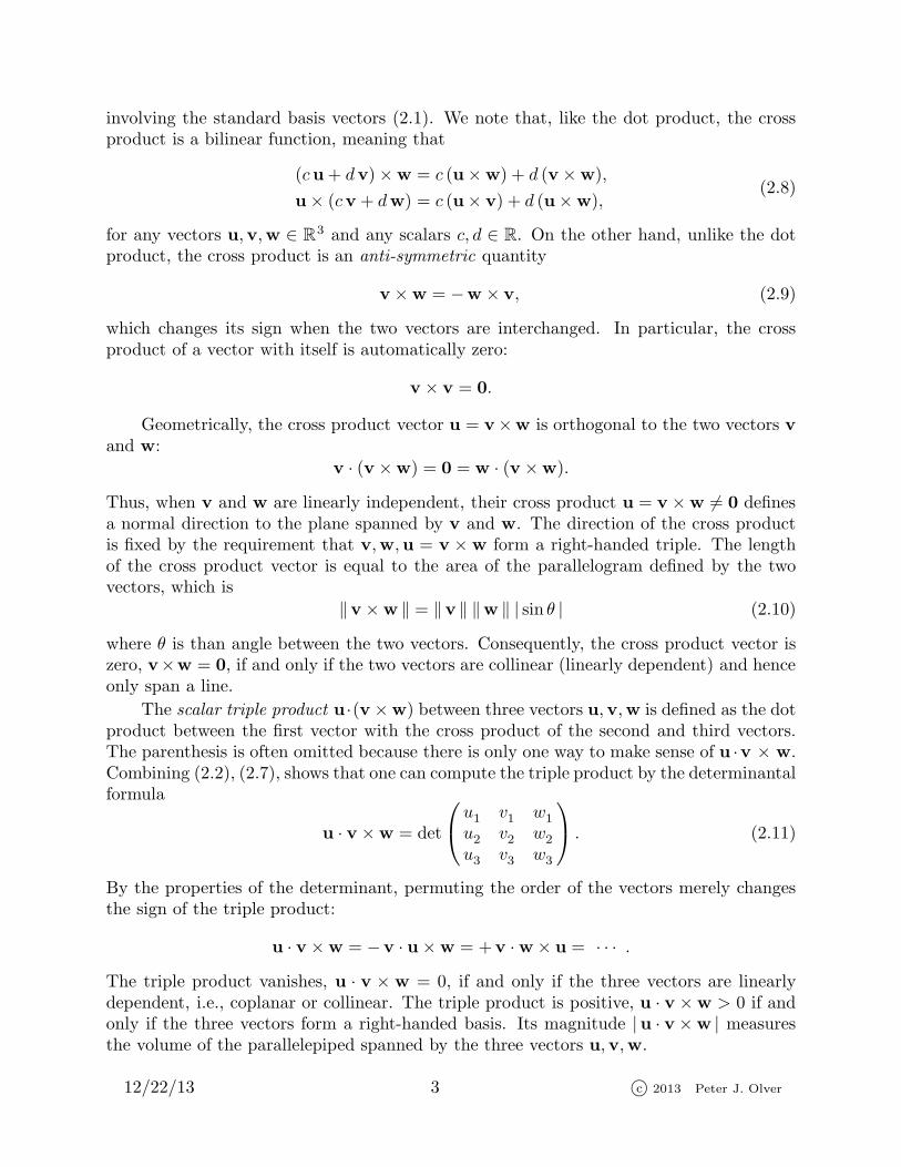
Figure 2. Two Views of a Trefoil Knot.

where c > 0 and ρ > 0 are positive constants. The curve describes a circular helix of radiusρ spiraling up the z axis. The parameter c determines the pitch of the helix, indicatinghow tightly its coils are wound; the smaller c is, the closer the winding. See Figure 1 foran illustration. DNA is, remarkably, formed in the shape of a (bent and twisted) doublehelix. The tangent to the helix at a point x(t) is the vector

x(t) =

−ρ sin tρ cos tc

.

Note that the speed of the particle,

‖

x ‖ =

√ρ2 sin2 t+ ρ2 cos2 t+ c2 =

√ρ2 + c2 , (3.4)

remains constant, although the velocity vector

x twists around.

A curve is simple if it never crosses itself, and closed if its ends meet, x(a) = x(b).In the plane, simple closed curves are all topologically equivalent, meaning one can becontinuously deformed to the other. In space, this is no longer true. Closed curves can beknotted, and thus have nontrivial topology.

Example 3.2. The curve

x(t) =

(2 + cos 3 t) cos 2 t(2 + cos 3 t) sin 2 t

sin 3 t

for 0 ≤ t ≤ 2π, (3.5)

describes a closed curve that is in the shape of a trefoil knot, as depicted in Figure 2. Thetrefoil is a genuine knot, meaning it cannot be deformed into an unknotted circle withoutcutting and retying. (However, a rigorous proof of this fact is not easy.) The trefoil is thesimplest of the “toroidal knots”.

12/22/13 5 c© 2013 Peter J. Olver

The study and classification of knots is a subject of great historical importance. In-deed, they were first considered from a mathematical viewpoint in the nineteenth century,when the English applied mathematician William Thompson (later Lord Kelvin) proposeda theory of atoms based on knots! In recent years, knot theory has witnessed a tremendousrevival, owing to its great relevance to modern day mathematics and physics. We refer theinterested reader to the advanced text [7] for details.

4. Line Integrals.

In this section, we discuss integrals along space curves.

Arc Length

The length of the space curve x(t) over the parameter range a ≤ t ≤ b is computedby integrating the norm of its tangent vector:

L(C) =∫ b

a

∥∥∥∥dx

dt

∥∥∥∥ dt =∫ b

a

√

x2 +

y2 +

z2 dt . (4.1)

It is not hard to show that the length of the curve is independent of the parametrization— as it should be.

Starting at the endpoint x(a), the arc length parameter s is given by

s =

∫ t

a

∥∥∥∥dx

dt

∥∥∥∥ dt and so ds = ‖

x ‖ dt =√

x2 +

y2 +

z2 dt. (4.2)

The arc length s measures the distance along the curve starting from the initial point x(a).Thus, the length of the part of the curve between s = α and s = β is exactly β − α. Itis often convenient to reparametrize the curve by its arc length, x(s). This has the sameeffect as moving along the curve at unit speed, since, by the chain rule,

dx

ds=dx

dt

dt

ds=

x

‖

x ‖ , so that

∥∥∥∥dx

ds

∥∥∥∥ = 1.

Therefore dx/ds is the unit tangent vector pointing in the direction of motion along thecurve.

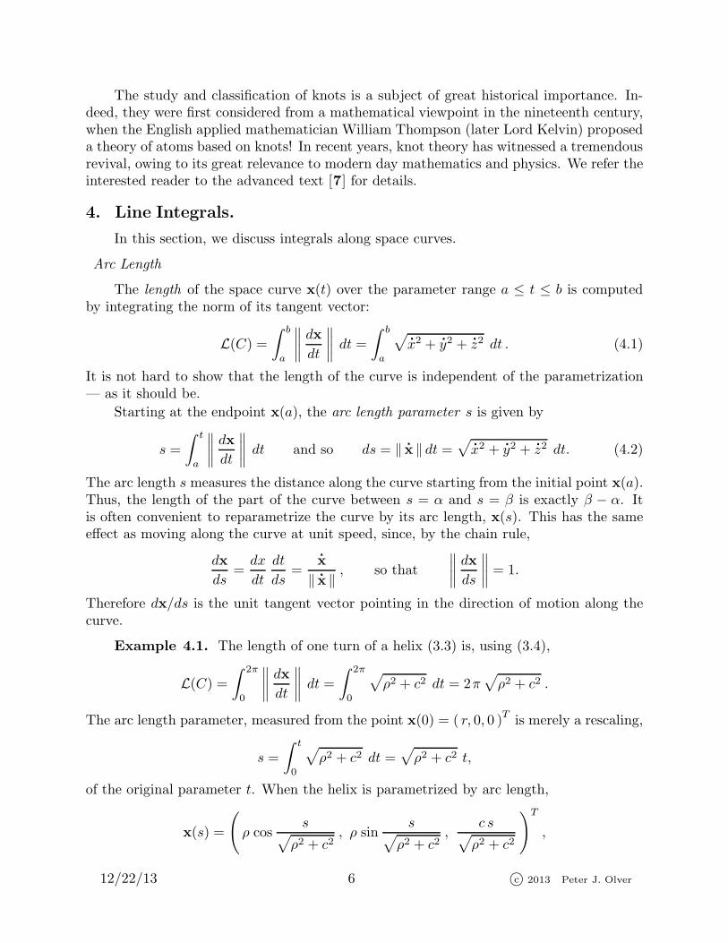
Example 4.1. The length of one turn of a helix (3.3) is, using (3.4),

L(C) =∫ 2π

0

∥∥∥∥dx

dt

∥∥∥∥ dt =∫ 2π

0

√ρ2 + c2 dt = 2π

√ρ2 + c2 .

The arc length parameter, measured from the point x(0) = ( r, 0, 0 )Tis merely a rescaling,

s =

∫ t

0

√ρ2 + c2 dt =

√ρ2 + c2 t,

of the original parameter t. When the helix is parametrized by arc length,

x(s) =

(ρ cos

s√ρ2 + c2

, ρ sins√

ρ2 + c2,

c s√ρ2 + c2

)T,

12/22/13 6 c© 2013 Peter J. Olver

we move along it with unit speed. It now takes time s = 2π√ρ2 + c2 to complete on turn

of the helix.

Example 4.2. To compute the length of the trefoil knot (3.5), we begin by comput-ing the tangent vector

dx

dt=

−2 (2 + cos 3 t) sin 2 t− 3 sin 3 t cos 2 t2 (2 + cos 3 t) cos 2 t− 3 sin 3 t sin 2 t

3 cos 3 t

.

After some algebra involving trigonometric identities, we find

‖

x ‖ =√27 + 16 cos 3 t+ 2 cos 6 t ,

which is never 0. Unfortunately, the resulting arc length integral

∫ 2π

0

‖

x ‖ dt =∫ 2π

0

√27 + 16 cos 3 t+ 2 cos 6 t dt

cannot be completed in elementary terms. Numerical integration can be used to find theapproximate value 31.8986 for the length of the knot.

The arc length integral of a scalar field u(x) = u(x, y, z) along a curve C is

∫

C

u ds =

∫ ℓ

0

u(x(s)) ds =

∫ ℓ

0

u(x(s), y(s), z(s))ds, (4.3)

where ℓ is the total length of the curve. For example, if ρ(x, y, z) represents the density at

position x = (x, y, z) of a wire bent in the shape of the curve C, then

∫

C

ρ ds represents

the total mass of the wire. In particular, the integral

∫

C

ds =

∫ ℓ

0

ds = ℓ

recovers the length of the curve.

If it is not convenient to work directly with the arc length parametrization, we can stillcompute the arc length integral in terms of the original parametrization x(t) for a ≤ t ≤ b.Using the change of parameter formula (4.2), we find

∫

C

u ds =

∫ b

a

u(x(t)) ‖

x ‖ dt =∫ b

a

u(x(t), y(t), z(t))√

x2 +

y2 +

z2 dt. (4.4)

Example 4.3. The density of a wire that is wound in the shape of a helix is propor-tional to its height. Let us compute the mass of one full turn of the helical wire. Thus,the density is given by ρ(x, y, z) = a z, where a is the constant of proportionality, and weare assuming z ≥ 0. Substituting into (4.4), the total mass of the wire is

L(C) =∫

C

a z ds =

∫ 2π

0

a c t√r2 + c2 dt = 2 π2 a c

√r2 + c2 .

12/22/13 7 c© 2013 Peter J. Olver

Line Integrals of Vector Fields

The line integral of a vector field v along a parametrized curve x(t) is obtained byintegration of its tangential component with respect to the arc length. The tangentialcomponent of v is given by

v · t, where t =dx

ds

is the unit tangent vector to the curve. Thus, the line integral of v is written as∫

C

v · dx =

∫

C

v1(x, y, z) dx+ v2(x, y, z) dy+ v3(x, y, z) dz =

∫

C

v · t ds. (4.5)

We can evaluate the line integral in terms of an arbitrary parametrization of the curve bythe general formula

∫

C

v · dx =

∫ b

a

v(x(t)) · dxdt

dt (4.6)

=

∫ b

a

[v1(x(t), y(t), z(t))

dx

dt+ v2(x(t), y(t), z(t))

dy

dt+ v3(x(t), y(t), z(t))

dz

dt

]dt.

Line integrals in three dimensions enjoy all of the properties of their two-dimensionalsiblings: Reversing the direction of parameterization along the curve changes the sign;also, the integral can be decomposed into sums over components:∫

−Cv · dx = −

∫

C

v · dx,∫

C

v · dx =

∫

C1

v · dx +

∫

C2

v · dx, C = C1 ∪ C2.

(4.7)

If f(x) represents a force field, e.g., gravity, electromagnetic force, etc., then its line

integral

∫

C

f · dx represents the work done by moving along the curve. As in two dimen-

sions, work is independent of the parametrization of the curve, i.e., the particle’s speed oftraversal.

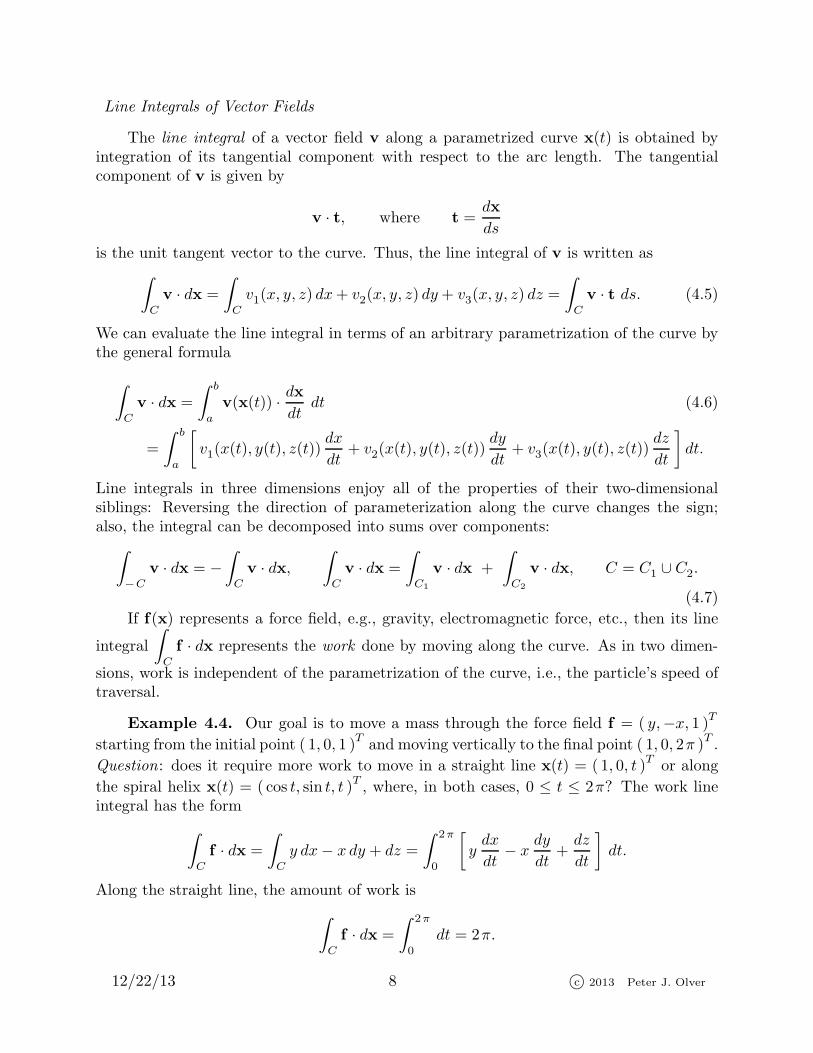
Example 4.4. Our goal is to move a mass through the force field f = ( y,−x, 1 )Tstarting from the initial point ( 1, 0, 1 )

Tand moving vertically to the final point ( 1, 0, 2π )

T.

Question: does it require more work to move in a straight line x(t) = ( 1, 0, t )Tor along

the spiral helix x(t) = ( cos t, sin t, t )T, where, in both cases, 0 ≤ t ≤ 2π? The work line

integral has the form

∫

C

f · dx =

∫

C

y dx− x dy + dz =

∫ 2π

0

[ydx

dt− x

dy

dt+dz

dt

]dt.

Along the straight line, the amount of work is

∫

C

f · dx =

∫ 2π

0

dt = 2π.

12/22/13 8 c© 2013 Peter J. Olver

As for the spiral helix,

∫

C

f · dx =

∫ 2π

0

[− sin2 t− cos2 t+ 1

]dt = 0.

Thus, although we travel a more roundabout route, it takes no work to move along thehelix!

The reason for the second result is that the force vector field f is everywhere orthogonalto the tangent to the curve: f · t = 0, and so there is no tangential force exerted upon themotion. In such cases, the work line integral

∫

C

f · dx =

∫

C

f · t ds = 0

automatically vanishes. In other words, it takes no work whatsoever to move in anydirection which is orthogonal to the given force vector.

5. Surfaces.

Curves are one-dimensional, and so can be traced out by a single parameter. Surfacesare two-dimensional, and hence require two distinct parameters. Thus, a surface S ⊂ R

3

is parametrized by a vector-valued function

x(p, q) = ( x(p, q), y(p, q), z(p, q) )T

(5.1)

that depends on two variables. As the parameters (p, q) ∈ Ω range over a prescribed planedomain Ω ⊂ R

2, the locus of points x(p, q) traces out the surface in space. The parametersare often thought of as defining a system of local coordinates on the curved surface.

We shall always assume that the surface is simple, meaning that it does not intersectitself, so x(p, q) = x(p, q) if and only if p = p and q = q. In practice, this condition can bequite hard to check! The boundary

∂S = x(p, q) | (p, q) ∈ ∂Ω (5.2)

of a simple surface consists of one or more simple curves. If the underlying parameterdomain Ω is bounded and simply connected, then ∂Ω is a simple closed plane curve, andso ∂S is also a simple closed curve.

Example 5.1. The simplest instance of a surface is a graph of a function. Theparameters are the x, y coordinates, and the surface coincides with the portion of thegraph of the function z = u(x, y) that lies over a fixed domain (x, y) ∈ Ω ⊂ R

2. Thus, agraphical surface has the parametric form

x(p, q) = ( p, q, u(p, q) )T, (p, q) ∈ Ω.

Thus, the parametrization identifies x = p and y = q, while z = u(p, q) = u(x, y) representsthe height of the surface above the point (x, y) ∈ Ω.

12/22/13 9 c© 2013 Peter J. Olver

x

y

z

r

ϕ

θ

(x, y, z)

(x, y, 0)

Figure 3. Spherical coordinates.

For example, the upper hemisphere S+r of radius r centered at the origin can be

parametrized as a graph

z =√r2 − x2 − y2, x2 + y2 < r2, (5.3)

sitting over the disk Dr = x2 + y2 < r2 of radius r. The boundary of the hemisphereis the image of the circle Cr = ∂Dr = x2 + y2 = r2 of radius r, and is itself a circle ofradius r sitting in the x, y plane: ∂S+

r = x2 + y2 = r, z = 0.

Example 5.2. A sphere Sr of radius r can be explicitly parametrized by two angularvariables ϕ, θ in the form

x(ϕ, θ) = (r sinϕ cos θ, r sinϕ sin θ, r cosϕ), 0 ≤ θ < 2π, 0 ≤ ϕ ≤ π. (5.4)

The reader can easily check that ‖x ‖2 = r2, as it should be. As illustrated in Figure 3, θmeasures the azimuthal angle or longitude, while ϕ measures the zenith angle or latitude.Thus, the upper hemisphere S+

r is obtained by restricting the zenith parameter to therange 0 ≤ ϕ ≤ 1

2 π. Each parameter value ϕ, θ corresponds to a unique point on thesphere, except when ϕ = 0 or π. All points (θ, 0) are mapped to the north pole ( 0, 0, r ),while all points (θ, π) are mapped to the south pole ( 0, 0,−r ). Away from the poles,the spherical angles provide bona fide coordinates on the sphere. Fortunately, the polarsingularities do not interfere with the overall smoothness of the sphere. Nevertheless, onemust always be careful at or near these two distinguished points.

Remark : In terrestrial cartography and navigation, the latitude is measured from theequator, and equals 1

2 π−ϕ, with positive values referring to the northern hemisphere andnegative the southern hemisphere (or, vice versa, if you are an antipodean). The longitudeis taken with respect to the prime meridian, through Greenwich, England, and equals π−θ,with positive values referring to the western hemisphere. Of course, in practice, both aremeasured in degrees rather than radians. The curves ϕ = c where the zenith angle takes

12/22/13 10 c© 2013 Peter J. Olver

a prescribed constant value are the circular parallels of constant latitude — except for thenorth and south poles which are merely points. The equator is at ϕ = 1

2π, while the tropics

of Cancer and Capricorn are 23 12

≈ 0.41 radians above and below the equator. The curvesθ = c where the meridial angle is constant are the semi-circular meridians of constantlongitude stretching from north to south pole. Note that θ = 0 and θ = 2π describe thesame meridian. In terrestrial navigation, latitude is the angle, in degrees, measured fromthe equator, while longitude is the angle measured from the Greenwich meridian.

Example 5.3. A torus is a surface of the form of an inner tube. One convenientparametrization of a particular toroidal surface is

x(ψ, θ) = ( (2 + cosψ) cos θ, (2 + cosψ) sin θ, sinψ )T

for 0 ≤ ψ, θ ≤ 2π. (5.5)

Note that the parametrization is 2π periodic in both ψ and θ. If we introduce cylindricalcoordinates

x = r cos θ, y = r sin θ, z,

then the torus is parametrized by

r = 2 + cosψ, z = sinψ.

Therefore, the relevant values of (r, z) all lie on the circle

(r − 2)2 + z2 = 1 (5.6)

of radius 1 centered at (2, 0). As the polar angle θ increases from 0 to 2π, the circle rotatesaround the z axis, and thereby sweeps out the torus.

Remark : The sphere and the torus are examples of closed surfaces . The requirementsfor a surface to be closed are that it be simple and bounded, and, moreover, have noboundary. In general, a subset S ⊂ R

3 is bounded provided it does not stretch off infinitelyfar away. More precisely, boundedness is equivalent to the existence of a fixed numberR > 0 which bounds the norm ‖x ‖ < R of all points x ∈ S.

Tangents to Surfaces

Consider a surface S parameterized by x(p, q) where (p, q) ∈ Ω. Each parametrizedcurve (p(t), q(t)) in the parameter domain Ω will be mapped to a parametrized curve C ⊂ Scontained in the surface. The curve C is parametrized by the composite map

x(t) = x(p(t), q(t)) = (x(p(t), q(t)), y(p(t), q(t)), z(p(t), q(t)) )T.

The tangent vectordx

dt=∂x

∂p

dp

dt+∂x

∂q

dq

dt(5.7)

to such a curve will be tangent to the surface. The set of all possible tangent vectors tocurves passing through a given point in the surface traces out the tangent plane to the

12/22/13 11 c© 2013 Peter J. Olver

surface at that point. Note that the tangent vector (5.7) is a linear combination of the twobasis tangent vectors

xp =∂x

∂p=

(∂x

∂p,∂y

∂p,∂z

∂p

)T, xq =

∂x

∂q=

(∂x

∂q,∂y

∂q,∂z

∂q

)T, (5.8)

which therefore span the tangent plane to the surface at the point x(p, q) ∈ S. The firstbasis vector is tangent to the curves where q = constant, while the second is tangent tothe curves where p = constant.

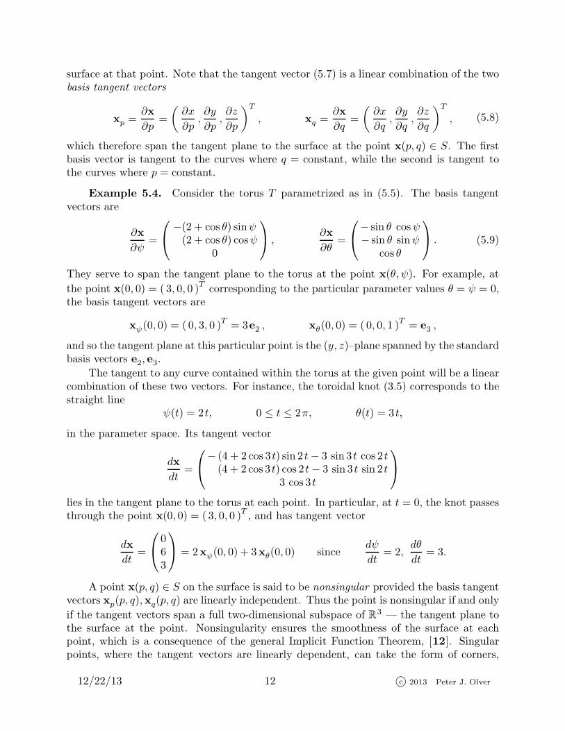
Example 5.4. Consider the torus T parametrized as in (5.5). The basis tangentvectors are

∂x

∂ψ=

−(2 + cos θ) sinψ(2 + cos θ) cosψ

0

,∂x

∂θ=

− sin θ cosψ− sin θ sinψ

cos θ

. (5.9)

They serve to span the tangent plane to the torus at the point x(θ, ψ). For example, at

the point x(0, 0) = ( 3, 0, 0 )Tcorresponding to the particular parameter values θ = ψ = 0,

the basis tangent vectors are

xψ(0, 0) = ( 0, 3, 0 )T= 3e2 , xθ(0, 0) = ( 0, 0, 1 )

T= e3 ,

and so the tangent plane at this particular point is the (y, z)–plane spanned by the standardbasis vectors e2, e3.

The tangent to any curve contained within the torus at the given point will be a linearcombination of these two vectors. For instance, the toroidal knot (3.5) corresponds to thestraight line

ψ(t) = 2 t, 0 ≤ t ≤ 2π, θ(t) = 3 t,

in the parameter space. Its tangent vector

dx

dt=

− (4 + 2 cos 3 t) sin 2 t− 3 sin 3 t cos 2 t(4 + 2 cos 3 t) cos 2 t− 3 sin 3 t sin 2 t

3 cos 3 t

lies in the tangent plane to the torus at each point. In particular, at t = 0, the knot passesthrough the point x(0, 0) = ( 3, 0, 0 )

T, and has tangent vector

dx

dt=

063

= 2xψ(0, 0) + 3xθ(0, 0) sincedψ

dt= 2,

dθ

dt= 3.

A point x(p, q) ∈ S on the surface is said to be nonsingular provided the basis tangentvectors xp(p, q),xq(p, q) are linearly independent. Thus the point is nonsingular if and only

if the tangent vectors span a full two-dimensional subspace of R3 — the tangent plane tothe surface at the point. Nonsingularity ensures the smoothness of the surface at eachpoint, which is a consequence of the general Implicit Function Theorem, [12]. Singularpoints, where the tangent vectors are linearly dependent, can take the form of corners,

12/22/13 12 c© 2013 Peter J. Olver

cusps and folds in the surface. From now on, we shall always assume that our surface isnonsingular meaning every point is a nonsingular point.

Linear independence of the tangent vectors is equivalent to the requirement that theircross product is a nonzero vector:

N =∂x

∂p× ∂x

∂q=

(∂(y, z)

∂(p, q),∂(z, x)

∂(p, q),∂(x, y)

∂(p, q)

)T6= 0. (5.10)

In this formula, we have adopted the standard notation

∂(x, y)

∂(p, q)= det

(xp xqyp yq

)=∂x

∂p

∂y

∂q− ∂x

∂q

∂y

∂p(5.11)

for the Jacobian determinant of the functions x, y with respect to the variables p, q. Thecross-product vector N in (5.10) is orthogonal to both tangent vectors, and hence orthog-onal to the entire tangent plane. Therefore, N defines a normal vector to the surface atthe given (nonsingular) point.

Example 5.5. Consider a surface S parametrized as the graph of a function z =u(x, y), and so, as in Example 5.1

x(x, y) = (x, y, u(x, y) )T, (x, y) ∈ Ω.

The tangent vectors

∂x

∂x=

(1, 0,

∂u

∂x

)T,

∂x

∂y=

(0, 1,

∂u

∂y

)T,

span the tangent plane sitting at the point (x, y, u(x, y) on S. The normal vector is

N =∂x

∂x× ∂x

∂y=

(− ∂u

∂x,− ∂u

∂y, 1

)T,

and points upwards. Note that every point on the graph is nonsingular.

The unit normal to the surface at the point is a unit vector orthogonal to the tangentplane, and hence given by

n =N

‖N ‖ =xp × xq

‖xp × xq ‖. (5.12)

In general, the direction of the normal vector N depends upon the order of the two param-eters p, q. Computing the cross product in the reverse order, xq × xp = −N, reverses thesign of the normal vector, and hence switches its direction. Thus, there are two possibleunit normals to the surface at each point, namely n and −n. For a closed surface, onenormal points outwards and one points inwards.

When possible, a consistent (meaning continuously varying) choice of a unit normalserves to define an orientation of the surface. All closed surfaces, and most other surfacescan be oriented. The usual convention for closed surfaces is to choose the orientationdefined by the outward normal. The simplest example of a non-orientable surface is theMobius strip obtained by gluing together the ends of a twisted strip of paper.

12/22/13 13 c© 2013 Peter J. Olver

Example 5.6. For the sphere of radius r parametrized by the spherical angles as in(5.4), the tangent vectors are

∂x

∂ϕ=

r cosϕ cos θr sinϕ cos θ− r sinϕ

, ∂x

∂θ=

− r sinϕ sin θr sinϕ cos θ

0

.

These vectors are tangent to, respectively, the meridians of constant longitude, and theparallels of constant latitude. The normal vector is

N =∂x

∂ϕ× ∂x

∂θ=

r2 sin2 ϕ cos θr2 sin2 ϕ sin θr2 cosϕ sinϕ

= r sinϕ x. (5.13)

Thus N is a non-zero multiple of the radial vector x, except at the north or south poleswhen ϕ = 0 or π. This reconfirms our earlier observation that the poles are problematicpoints for the spherical angle parametrization. The unit normal

n =N

‖N ‖ =x

r

determined by the spherical coordinates ϕ, θ is the outward pointing normal. Reversingthe order of the angles, θ, ϕ, would lead to the outwards normal −n = −x/r.

Remark : As we already saw in the example of the hemisphere, a given surface can beparametrized in many different ways. In general, to change parameters

p = g(p, q), q = h(p, q),

requires a smooth, invertible map between the two parameter domains Ω → Ω. Manyinteresting surfaces, particularly closed surfaces, cannot be parametrized in a single con-sistent manner that satisfies the smoothness constraint (5.10) on the entire surface. Insuch cases, one must assemble the surface out of pieces, each parametrized in the propermanner. The key problem in cartography is to find convenient parametrizations of theglobe that do not significantly distort the geographical features of the planet.

A surface is piecewise smooth if it can be constructed by gluing together a finitenumber of smooth parts, joined along piecewise smooth curves. For example, a cube isa piecewise smooth surface, consisting of squares joined along straight line segments. Weshall rely on the reader’s intuition to formalize these ideas, leaving a rigorous developmentto a more comprehensive treatment of surface geometry, e.g., [5].

6. Surface Integrals.

As with spatial line integrals, there are two important types of surface integral. Thefirst is the integration of a scalar field with respect to surface area. A typical applicationis to compute the area of a curved surface or the mass and center of mass of a curved shellof possibly variable density. The second type is the surface integral that computes the flux

12/22/13 14 c© 2013 Peter J. Olver

associated with a vector field through an oriented surface. Applications appear in fluidmechanics, electromagnetism, thermodynamics, gravitation, and many other fields.

Surface Area

According to (2.10), the length of the cross product of two vectors measures the areaof the parallelogram they span. This observation underlies the proof that the length of thenormal vector to a surface (5.12), namely

‖N ‖ = ‖xp × xq ‖,is a measure of the infinitesimal element of surface area, denoted

dS = ‖N ‖ dp dq = ‖xp × xq ‖ dp dq. (6.1)

The total area of the surface is found by summing up these infinitesimal contributions,and is therefore given by the double integral

area S =

∫ ∫

S

dS =

∫ ∫

Ω

‖xp × xq ‖ dp dq

=

∫ ∫

Ω

√(∂(y, z)

∂(p, q)

)2

+

(∂(z, x)

∂(p, q)

)2

+

(∂(x, y)

∂(p, q)

)2

dp dq.

(6.2)

The surface’s area does not depend upon the parametrization used to compute the integral.In particular, if the surface is parametrized by x, y as the graph z = u(x, y) of a functionover a domain (x, y) ∈ Ω, then the surface area integral reduces to the familiar form

area S =

∫ ∫

S

dS =

∫ ∫

Ω

√

1 +

(∂u

∂x

)2

+

(∂u

∂y

)dx dy. (6.3)

A detailed justification of these formulae can be found in [1, 6, 9].

Example 6.1. The well-known formula for the surface area of a sphere is a simpleconsequence of the integral formula (6.2). Using the parametrization by spherical angles(5.4) and the formula (5.13) for the normal, we find

area Sr =

∫ ∫

Sr

dS =

∫ 2π

0

∫ π

0

r2 sinϕ dϕdθ = 4 π r2. (6.4)

Fortunately, the problematic poles do not cause any difficulty in the computation, sincethey contribute nothing to the surface area integral.

Alternatively, we can compute the area of one hemisphere S+r by realizing it as a

graph

z =√r2 − x2 − y2 for x2 + y2 ≤ 1,

over the disk of radius r, and so, by (6.3),

area S+r =

∫ ∫

Ω

√

1 +x2

r2 − x2 − y2+

y2

r2 − x2 − y2dx dy

=

∫ ∫

Ω

r√r2 − x2 − y2

dx dy =

∫ r

0

∫ 2π

0

r ρ√r2 − ρ2

dθ dρ = 2 π r2,

12/22/13 15 c© 2013 Peter J. Olver

where we used polar coordinates x = ρ cos θ, y = ρ sin θ to evaluate the final integral. Thearea of the entire sphere is twice the area of the hemisphere.

Example 6.2. Similarly, to compute the surface area of the torus T parametrizedin (5.5), we use the tangent vectors in (5.9) to compute the normal to the torus:

N = xψ × xθ =

(2 + cosψ) cosψ cos θ(2 + cosψ) cosψ sin θ

(2 + cosψ) sinψ

, with ‖xψ × xθ ‖ = 2 + cosψ.

Therefore,

area T =

∫ 2π

0

∫ 2π

0

(2 + cosψ) dψ dθ = 8 π2.

If S ⊂ R3 is a surface with finite area, the mean or average of a scalar function

f(x, y, z) over S is given by

MS [ f ] =1

area S

∫ ∫

S

f dS. (6.5)

For example, the mean of a function over a sphere Sr = ‖x ‖ = r of radius r is explicitlygiven by

MSr[ f ] =

1

4πr2

∫ ∫

‖x ‖=rf(x) dS =

1

4π

∫ 2π

0

∫ π

0

F (r, ϕ, θ) sinϕdϕdθ, (6.6)

where F (r, ϕ, θ) is the spherical coordinate expression for the scalar function f . As usual,the mean lies between the maximum and minimum values of the function on the surface:

minSf ≤ MS [ f ] ≤ max

Sf.

In particular, the center of mass C of a surface (assuming it has constant density) is equal

to the mean of the coordinate functions x = (x, y, z )T, so

C = (MS [x ] ,MS [ y ] ,MS [ z ] )T=

1

area S

(∫ ∫

S

x dS,

∫ ∫

S

y dS,

∫ ∫

S

z dS

)T. (6.7)

More generally, the integral of a scalar field u(x, y, z) over the surface is given by∫ ∫

S

u dS =

∫ ∫

Ω

u(x(p, q), y(p, q), z(p, q)) ‖xp × xq ‖ dp dq. (6.8)

If S represents a thin curved shell, and u = ρ(x) the density of the material at positionx ∈ S, then the surface integral (6.8) represents the total mass of the shell. For example,the integral of u(x, y, z) over a hemisphere S+

r of radius r can be evaluated by either ofthe formulae

∫ ∫

S+r

u dS =

∫ 2π

0

∫ π/2

0

u(r cos θ sinϕ, r sin θ sinϕ, r cosϕ) r2 sinϕ dϕdθ

=

∫ ∫

x2+y2≤r2

r√r2 − x2 − y2

u(x, y,√r2 − x2 − y2 ) dx dy,

(6.9)

12/22/13 16 c© 2013 Peter J. Olver

depending upon whether one prefers spherical or graphical coordinates.

Flux Integrals

Now assume that S is an oriented surface with chosen unit normal n. If v = (u, v, w )T

is a vector field, then the surface integral

∫ ∫

S

v · n dS =

∫ ∫

Ω

(v · xp × xq

)dp dq =

∫ ∫

Ω

det

u xp xqv yp yqw zp zq

dp dq (6.10)

of the normal component of v over the entire surface measures its flux through the surface.An alternative common notation for the flux integral is

∫ ∫

S

v · n dS =

∫ ∫

S

u dy dz + v dz dx+ w dx dy (6.11)

=

∫ ∫

Ω

(u(x, y, z)

∂(y, z)

∂(p, q)+ v(x, y, z)

∂(z, x)

∂(p, q)+ w(x, y, z)

∂(x, y)

∂(p, q)

)dx dy,

Note how the Jacobian determinant notation (5.11) seamlessly interacts with the integra-tion. In particular, if the surface is the graph of a function z = h(x, y), then the surfaceintegral reduces to the particularly simple form

∫ ∫

S

v · n dS =

∫ ∫

Ω

(u(x, y, z)

∂z

∂x+ v(x, y, z)

∂z

∂y+ w(x, y, z)

)dp dq (6.12)

The flux surface integral relies upon the consistent choice of an orientation or unitnormal on the surface. Thus, flux only makes sense through an oriented surface — itdoesn’t make sense to speak of “flux through a Mobius band”. If we switch normals,using, say, the inward instead of the outward normal, then the surface integral changessign — just like a line integral if we reverse the orientation of a curve. Similarly, if wedecompose a surface into the union of two or more parts, with only their boundaries incommon, then the surface integral similarly decomposes into a sum of surface integrals.Thus,

∫ ∫

−Sv · n dS = −

∫ ∫

S

v · n dS,

∫ ∫

S

v · n dS =

∫ ∫

S1

v · n dS +

∫ ∫

S2

v · n dS, S = S1 ∪ S2.

(6.13)

In the first formula, −S denotes the surface S with the reverse orientation. In the secondformula, S1 and S2 are only allowed to intersect along their boundaries; moreover, theymust be oriented in the same manner as S, i.e., have the same unit normal direction.

Example 6.3. Let S denote the triangular surface given by that portion of the planex+ y + z = 1 that lies inside the positive orthant x ≥ 0, y ≥ 0, z ≥ 0. The flux of the

vector field v = ( y, xz, 0 )Tthrough S equals the surface integral

∫ ∫

S

y dy dz + xz dz dx,

12/22/13 17 c© 2013 Peter J. Olver

where we orient S by choosing the upwards pointing normal. To compute, we note thatS can be identified as the graph of the function z = 1 − x − y lying over the triangleT = 0 ≤ x ≤ 1, 0 ≤ y ≤ 1− x. Therefore, by (6.11),

∫ ∫

S

y dy dz + x z dz dx =

∫ ∫

T

[y∂(y, 1− x− y)

∂(x, y)+ x (1− x− y)

∂(1− x− y, x)

∂(x, y)

]dx dy

=

∫ 1

0

∫ 1−x

0

(1− x) (y + x) dy dx =

∫ 1

0

(12 + 1

2 x− 12 x

2 + 12 x

3)dx = 17

24 .

If v represents the velocity vector field for a steady state fluid flow, then its fluxintegral (6.10) tells us the total volume of fluid passing through S per unit time. Indeed,at each point on S, the volume fluid that flows across a small part the surface in unittime will fill a thin cylinder whose base is the surface area element dS and whose heightv ·n is the normal component of the fluid velocity v. Summing (integrating) all these fluxcylinder volumes over the surface results in the flux integral. The choice of orientation orunit normal specifies the convention for measuring the direction of positive flux throughthe surface. If S is a closed surface, and we choose n to be the unit outward normal, thenthe flux integral (6.10) represents the net amount of fluid flowing out of the solid regionbounded by S per unit time.

Example 6.4. The vector field v = ( 0, 0, 1 )T

represents a fluid moving with con-stant velocity in the vertical direction. Let us compute the fluid flux through a hemisphere

S+r =

z =

√r2 − x2 − y2

∣∣∣ x2 + y2 ≤ 1,

sitting over the disk Dr of radius r in the x, y plane. The flux integral over S+r is computed

using (6.12), so

∫ ∫

S+r

v · n dS =

∫ ∫

S+r

dx× dy =

∫ ∫

Dr

dx dy = πr2.

The resulting double integral is just the area of the disk. Indeed, in this case, the value ofthe flux integral is the same for all surfaces z = h(x, y) sitting over the disk Dr.

This example provides a particular case of a surface-independent flux integral, whichare defined in analogy with the path-independent line integrals that we encountered earlier.In general, a flux integral is called surface-independent if

∫ ∫

S1

v · n dS =

∫ ∫

S2

v · n dS (6.14)

whenever the surfaces S1 and S2 have a common boundary ∂S1 = ∂S2. In other words,the value of the integral depends only upon the boundary of the surface. The veracity of(6.14) requires that the surfaces be oriented in the “same manner”. For instance, if theydo not cross, then the combined surface S = S1 ∪ S2 is closed, and one uses the outwardpointing normal on one surface and the inward pointing normal on the other. In morecomplex situations, one checks that the two surfaces induce the same orientation on their

12/22/13 18 c© 2013 Peter J. Olver

common boundary. (We defer a discussion of the boundary orientation until later.) Finally,applying (6.13) to the closed surface S = S1 ∪ S2 and using the prescribed orientations,we deduce an alternative characterization of surface-independent vector fields.

Proposition 6.5. A vector field leads to a surface-independent flux integral if and

only if ∫ ∫

S

v · n dS = 0 (6.15)

for every closed surface S contained in the domain of definition of v.

A fluid is incompressible when its volume is unaltered by the flow. Therefore, in theabsence of sources or sinks, there cannot be any net inflow or outflow across a simple closedsurface bounding a region occupied by the fluid. Thus, the flux integral over a closed surface

must vanish:

∫ ∫

S

v · n dS = 0. Proposition 6.5 implies that the fluid velocity vector field

defines a surface-independent flux integral. Thus, the flux of an incompressible fluid flowthrough any surface depends only on the (oriented) boundary curve of the surface!

7. Volume Integrals.

Volume or triple integrals take place over domains Ω ⊂ R3 representing solid three-

dimensional bodies. A simple example of such a domain is a ball

Br(a) = x | ‖x− a ‖ < r (7.1)

of radius r > 0 centered at a point a ∈ R3. Other examples of domains include solid cubes,

solid cylinders, solid tetrahedra, solid tori (doughnuts and bagels), solid cones, etc.

In general, a subset Ω ⊂ R3 is open if, for every point x ∈ Ω, a small open ball

Bε(a) ⊂ Ω centered at a of radius ε = ε(a) > 0, which may depend upon a, is alsocontained in Ω. In particular, the ball (7.1) is open. The boundary ∂Ω of an open subsetΩ consists of all limit points which are not in the subset. Thus, the boundary of the openball Br(a) is the sphere Sr(a) = ‖x− a ‖ = r of radius r centered at the point a. Anopen subset is called a domain if its boundary ∂Ω consists of one or more simple, piecewisesmooth surfaces. We are allowing corners and edges in the bounding surfaces, so that anopen cube will be a perfectly valid domain.

A subset Ω ⊂ R3 is bounded provided it fits inside a sphere of some (possibly large)

radius. For example, the solid ball Br = ‖x ‖ < R is bounded, while its exterior Er =‖x ‖ > R is an unbounded domain. The sphere SR = ‖x ‖ = R is the commonboundary of the two domains: SR = ∂Br = ∂ER. Indeed, any simple closed surfaceseparates R

3 into two domains that have a common boundary — its interior , which isbounded, and its unbounded exterior .

The boundary of a bounded domain consists of one or more closed surfaces. Forinstance, the solid annular domain

Ar,R =0 < r < ‖x ‖ < R

(7.2)

12/22/13 19 c© 2013 Peter J. Olver

consisting of all points lying between two concentric spheres of respective radii r and Rhas boundary given by the two spheres: ∂Ar,R = Sr ∪ SR. On the other hand, settingr = 0 in (7.2) leads to a punctured ball of radius R whose center point has been removed.A punctured ball is not a domain, since the center point is part of the boundary, but isnot a bona fide surface.

If the domain Ω ⊂ R3 represents a solid body, and the scalar field ρ(x, y, z) represents

its density at a point (x, y, z) ∈ Ω, then the triple integral

∫ ∫ ∫

Ω

ρ(x, y, z)dx dy dz (7.3)

equals the total mass of the body. In particular, the volume of Ω is equal to

volΩ =

∫ ∫ ∫

Ω

dx dy dz. (7.4)

Triple integrals can be directly evaluated when the domain has the particular form

Ω =ξ(x, y) < z < η(x, y), ϕ(x) < y < ϕ(x), a < x < b

(7.5)

where the z coordinate lies between two graphical surfaces sitting over a common domainin the (x, y)–plane that is itself of the form of (7.5) used to evaluate double integrals. Insuch cases we can evaluate the triple integral by iterated integration first with respect toz, then with respect to y and, finally, with respect to x:

∫ ∫ ∫

Ω

u(x, y, z)dx dy dz =

∫ b

a

(∫ ψ(x)

ϕ(x)

(∫ η(x,y)

ξ(x,y)

u(x, y, z)dz

)dy

)dx. (7.6)

A similar result holds for other orderings of the coordinates.

Fubini’s Theorem, [11, 12], assures us that the result of iterated integration does notdepend upon the order in which the variables are integrated. Of course, the domain mustbe of the requisite type in order to write the volume integral as repeated single integrals.More general triple integrals can be evaluated by chopping the domain up into disjointpieces that have the proper form.

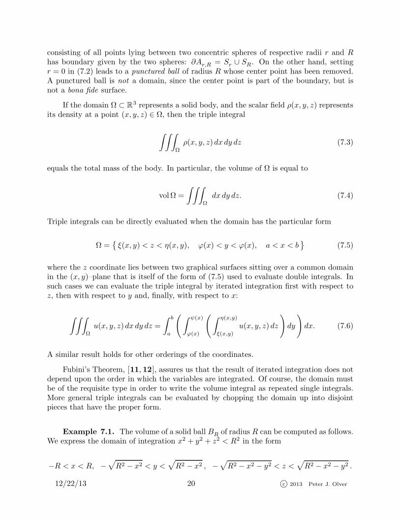
Example 7.1. The volume of a solid ball BR of radius R can be computed as follows.We express the domain of integration x2 + y2 + z2 < R2 in the form

−R < x < R, −√R2 − x2 < y <

√R2 − x2 , −

√R2 − x2 − y2 < z <

√R2 − x2 − y2 .

12/22/13 20 c© 2013 Peter J. Olver

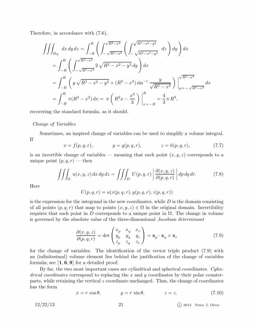
Therefore, in accordance with (7.6),

∫ ∫ ∫

BR

dx dy dz =

∫ R

−R

(∫ √R2−x2

−√R2−x2

(∫ √R2−x2−y2

−√R2−x2−y2

dz

)dy

)dx

=

∫ R

−R

(∫ √R2−x2

−√R2−x2

2√R2 − x2 − y2 dy

)dx

=

∫ R

−R

(y√R2 − x2 − y2 + (R2 − x2) sin−1 y√

R2 − x2

) ∣∣∣∣

√R2−x2

y=−√R2−x2

dx

=

∫ R

−Rπ(R2 − x2) dx = π

(R2x− x3

3

) ∣∣∣∣R

x=−R=

4

3πR3,

recovering the standard formula, as it should.

Change of Variables

Sometimes, an inspired change of variables can be used to simplify a volume integral.If

x = f(p, q, r), y = g(p, q, r), z = h(p, q, r), (7.7)

is an invertible change of variables — meaning that each point (x, y, z) corresponds to aunique point (p, q, r) — then

∫ ∫ ∫

Ω

u(x, y, z)dx dy dz =

∫ ∫ ∫

D

U(p, q, r)

∣∣∣∣∂(x, y, z)

∂(p, q, r)

∣∣∣∣ dp dq dr. (7.8)

HereU(p, q, r) = u(x(p, q, r), y(p, q, r), z(p, q, r))

is the expression for the integrand in the new coordinates, while D is the domain consistingof all points (p, q, r) that map to points (x, y, z) ∈ Ω in the original domain. Invertibilityrequires that each point in D corresponds to a unique point in Ω. The change in volumeis governed by the absolute value of the three-dimensional Jacobian determinant

∂(x, y, z)

∂(p, q, r)= det

xp xq xryp yq yrzp zq zr

= xp · xq × xr (7.9)

for the change of variables. The identification of the vector triple product (7.9) withan (infinitesimal) volume element lies behind the justification of the change of variablesformula; see [1, 6, 9] for a detailed proof.

By far, the two most important cases are cylindrical and spherical coordinates. Cylin-drical coordinates correspond to replacing the x and y coordinates by their polar counter-parts, while retaining the vertical z coordinate unchanged. Thus, the change of coordinateshas the form

x = r cos θ, y = r sin θ, z = z. (7.10)

12/22/13 21 c© 2013 Peter J. Olver

The Jacobian determinant for cylindrical coordinates is

∂(x, y, z)

∂(r, θ, z)= det

xr xθ xzyr yθ yzzr zθ zz

= det

cos θ −r sin θ 0sin θ r cos θ 00 0 1

= r. (7.11)

Therefore, the general change of variables formula (7.8) tells us the formula for a tripleintegral in cylindrical coordinates:

∫ ∫ ∫f(x, y, z)dx dy dz =

∫ ∫ ∫f(r cos θ, r sin θ, z) r dr dθ dz. (7.12)

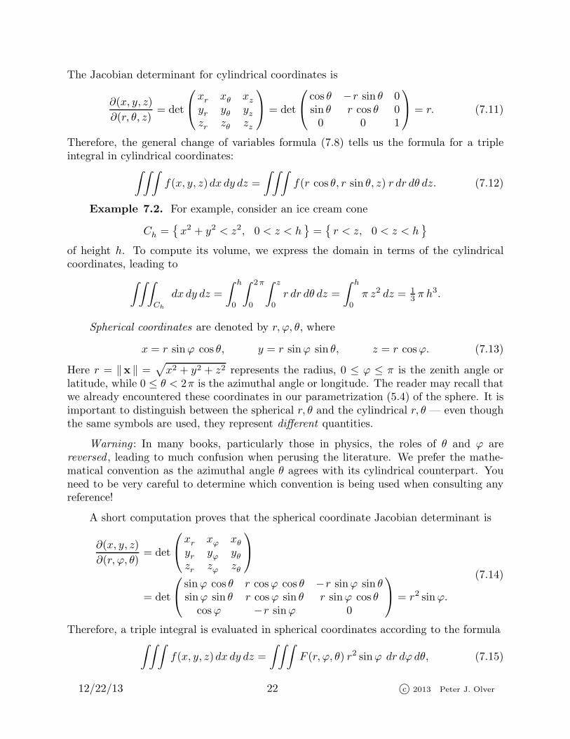
Example 7.2. For example, consider an ice cream cone

Ch =x2 + y2 < z2, 0 < z < h

=r < z, 0 < z < h

of height h. To compute its volume, we express the domain in terms of the cylindricalcoordinates, leading to

∫ ∫ ∫

Ch

dx dy dz =

∫ h

0

∫ 2π

0

∫ z

0

r dr dθ dz =

∫ h

0

π z2 dz = 13 π h

3.

Spherical coordinates are denoted by r, ϕ, θ, where

x = r sinϕ cos θ, y = r sinϕ sin θ, z = r cosϕ. (7.13)

Here r = ‖x ‖ =√x2 + y2 + z2 represents the radius, 0 ≤ ϕ ≤ π is the zenith angle or

latitude, while 0 ≤ θ < 2π is the azimuthal angle or longitude. The reader may recall thatwe already encountered these coordinates in our parametrization (5.4) of the sphere. It isimportant to distinguish between the spherical r, θ and the cylindrical r, θ — even thoughthe same symbols are used, they represent different quantities.

Warning : In many books, particularly those in physics, the roles of θ and ϕ arereversed , leading to much confusion when perusing the literature. We prefer the mathe-matical convention as the azimuthal angle θ agrees with its cylindrical counterpart. Youneed to be very careful to determine which convention is being used when consulting anyreference!

A short computation proves that the spherical coordinate Jacobian determinant is

∂(x, y, z)

∂(r, ϕ, θ)= det

xr xϕ xθyr yϕ yθzr zϕ zθ

= det

sinϕ cos θ r cosϕ cos θ −r sinϕ sin θsinϕ sin θ r cosϕ sin θ r sinϕ cos θ

cosϕ −r sinϕ 0

= r2 sinϕ.

(7.14)

Therefore, a triple integral is evaluated in spherical coordinates according to the formula∫ ∫ ∫

f(x, y, z)dx dy dz =

∫ ∫ ∫F (r, ϕ, θ) r2 sinϕ dr dϕ dθ, (7.15)

12/22/13 22 c© 2013 Peter J. Olver

where we rewrite the integrand

F (r, ϕ, θ) = f(r sinϕ cos θ, r sinϕ sin θ, r cosϕ) (7.16)

as a function of the spherical coordinates.

Example 7.3. The integration required in Example 7.1 to compute the volumeof a ball BR of radius R can be considerably simplified by switching over to sphericalcoordinates. The ball is given by BR =

0 ≤ r < R, 0 ≤ ϕ ≤ π, 0 ≤ θ < 2π

. Thus, using

(7.15), we compute

∫ ∫ ∫

BR

dx dy dz =

∫ R

0

∫ π

0

∫ 2π

0

r2 sinϕ dθ dϕ dr =

∫ R

0

4π r2 dr = 43 π R

3. (7.17)

The reader may note that the next-to-last integrand represents the surface area of thesphere of radius R. Thus, we are, in effect, computing the volume by summing up (i.e.,integrating) the surface areas of concentric thin spherical shells.

Remark : Sometimes, we will be sloppy and use the same letter for a function in analternative coordinate system. Thus, we may use f(r, ϕ, θ) to represent the sphericalcoordinate form (7.16) of a function f(x, y, z). Technically, this is not correct! However,the clarity and intuition sometimes outweighs the pedantic use of a new letter each time wechange coordinates. Moreover, in geometry and modern physical theories, [2], the symbol“f” represents an intrinsic scalar field, and f(x, y, z) and f(r, ϕ, θ) merely its incarnationsin two different coordinate charts on R

3. Hopefully, this will be clear from the context.

8. Gradient, Divergence, and Curl.

There are three important vector differential operators that play a ubiquitous role inthree-dimensional vector calculus, known as the gradient, divergence and curl.

The Gradient

We begin with the three-dimensional version of the gradient operator

∇u =

uxuyuz

. (8.1)

The gradient defines a linear operator that maps a scalar function u(x, y, z) to the vectorfield whose components are its partial derivatives with respect to the Cartesian coordinates.

If x(t) = (x(t), y(t), z(t) )Tis any parametrized curve, then the rate of change in the

function u as we move along the curve is given by the inner product

d

dtu(x(t), y(t), z(t)) =

∂u

∂x

dx

dt+∂u

∂y

dy

dt+∂u

∂z

dz

dt= ∇u ·

x (8.2)

between the gradient and the tangent vector to the curve. Therefore, as we reasonedearlier in the planar case, the gradient ∇u points in the direction of steepest increase inthe function u, while its negative −∇u points in the direction of steepest decrease. For

12/22/13 23 c© 2013 Peter J. Olver

example, if u(x, y, z) represents the temperature at a point (x, y, z) in space, then ∇upoints in the direction in which temperature is getting the hottest, while −∇u points inthe direction it gets the coldest. Therefore, if one wants to cool down as rapidly as possible,one should move in the direction of −∇u at each instant, which is the direction of theflow of heat energy. Thus, the path x(t) to be followed for the fastest cool down will be asolution to the gradient flow equations

x = −∇u, (8.3)

or, explicitly,

dx

dt= − ∂u

∂x(x, y, z),

dy

dt= − ∂u

∂y(x, y, z),

dz

dt= − ∂u

∂z(x, y, z).

A solution x(t) to such a system of ordinary differential equations will experience continu-ously decreasing temperature. One can use such gradient flows to locate and numericallyapproximate the minima of functions, [4].

The set of all points where a scalar field u(x, y, z) has a given value,

u(x, y, z) = c (8.4)

for some fixed constant c, is known as a level set of u. If u measures temperature, thenits level sets are the isothermal surfaces of equal temperature. If u is sufficiently smooth,most of its level sets are smooth surfaces. In fact, if ∇u 6= 0 at a point, then one can provethat all nearby level sets are smooth surfaces near the point in question. This importantfact is a consequence of the general Implicit Function Theorem, [12]. Thus, if ∇u 6= 0 atall points on a level set, then the level set is a smooth surface, and, if bounded, a simpleclosed surface. (On the other hand, finding an explicit parametrization of a level set maybe quite difficult!)

Theorem 8.1. If nonzero, the gradient vector ∇u 6= 0 defines the normal direction

to the level set u = c at each point.

Proof : Indeed, suppose x(t) is any curve contained in the level set, so that

u(x(t), y(t), z(t)) = c for all t.

Since c is constant, the derivative with respect to t is zero, and hence, by (8.2),

d

dtu(x(t), y(t), z(t)) = ∇u ·

x = 0,

which implies that the gradient vector ∇u is orthogonal to the tangent vector

x to thecurve. Since this holds for all such curves contained within the level set, the gradient mustbe orthogonal to the entire tangent plane at the point, and hence, if nonzero, defines anormal direction to the level surface. Q.E.D.

12/22/13 24 c© 2013 Peter J. Olver

Physically, Theorem 8.1 tells us that the direction of steepest increase in temperatureis perpendicular to the isothermal surfaces at each point. Consequently, the solutions tothe gradient flow equations (8.3) form an orthogonal system of curves to the level setsurfaces of u, and one should follow these curves to minimize the temperature as rapidlyas possible. Similarly, in a steady state fluid flow, the fluid potential is represented by ascalar field ϕ(x, y, z). Its gradient v = ∇ϕ determines the fluid velocity at each point. Thestreamlines followed by the fluid particles are the solutions to the gradient flow equations

x = v = ∇ϕ, while the level sets of ϕ are the equipotential surfaces. Thus, fluid particlesflow in a direction orthogonal to the equipotential surfaces.

Example 8.2. The level sets of the radial function u = x2+y2+z2 are the concentricspheres centered at the origin. Its gradient ∇u = ( 2x, 2y, 2z )

T= 2x points in the radial

direction, orthogonal to each spherical level set. Note that ∇u = 0 only at the origin,which is a level set, but not a smooth surface.

The radial vector also specifies the direction of fastest increase (decrease) in the func-tion u. Indeed, the solution to the associated gradient flow system (8.3), namely

x = − 2x is x(t) = x0 e−2 t,

where x0 = x(0) is the initial position. Therefore, to decrease the function u as rapidly aspossible, one should follow a radial ray into the origin.

Example 8.3. An implicit equation for the torus (5.5) is obtained by replacing

r =√x2 + y2 in (5.6). In this manner, we are led to consider the level sets of the function

u(x, y, z) = x2 + y2 + z2 − 4√x2 + y2 = c, (8.5)

with the particular value c = −3 corresponding to (5.5). The gradient of the function is

∇u(x, y, z) =(2x− 4x√

x2 + y2, 2y − 4y√

x2 + y2, 2z

)T, (8.6)

which is well-define except on the z axis, where x = y = 0. Note that ∇F 6= 0 unless z = 0and x2 + y2 = 4. Therefore, the level sets of u are smooth, toroidal surfaces except for zaxis and the circle of radius 2 in the (x, y) plane.

Divergence and Curl

The second important vector differential operator is the divergence,

divv = ∇ · v =∂v1∂x

+∂v2∂y

+∂v3∂z

. (8.7)

The divergence maps a vector field v = ( v1, v2, v3 )T

to a scalar field f = ∇ · v. For

example, the radial vector field v = (x, y, z )Thas constant divergence ∇ · v = 3.

In fluid mechanics, the divergence measures the local, instantaneous change in thevolume of a fluid packet as it moves. Thus, a steady state fluid flow is incompressible, with

12/22/13 25 c© 2013 Peter J. Olver

unchanging volume, if and only if its velocity vector field is divergence-free: ∇·v ≡ 0. Theconnection between incompressibility and the earlier zero-flux condition will be addressedin the Divergence Theorem 9.6 below.

As in the two-dimensional situation, the composition of divergence and gradient pro-duces the Laplacian operator:

∇ · ∇u = ∆u = uxx + uyy + uzz. (8.8)

Indeed, as we shall see, except for the missing minus sign and the all-important boundaryconditions, this is effectively the same as the self-adjoint form of the three-dimensionalLaplacian:

∇∗ ∇u = −∇ · ∇u = −∆u.

The third important vector differential operator is the curl , which, in three dimensions,maps vector fields to vector fields. It is most easily memorized in the form of a (formal)3× 3 determinant

curlv = ∇× v =

∂v3∂y

− ∂v2∂z

∂v1∂z

− ∂v3∂x

∂v2∂x

− ∂v1∂y

= det

∂x v1 e1∂y v2 e2∂z v3 e3

, (8.9)

in analogy with the determinantal form (2.6) of the cross product. For instance, the radial

vector field v = (x, y, z )Thas zero curl:

∇× v = det

∂x x e1∂y y e2∂z z e3

= 0.

This is indicative of the lack or any rotational effect of the induced flow.

If v represents the velocity vector field of a steady state fluid flow, its curl ∇ × v

measures the instantaneous rotation of the fluid flow at a point, and is known as thevorticity of the flow. When non-zero, the direction of the vorticity vector represents theaxis of rotation, while its magnitude ‖∇× v ‖ measures the instantaneous angular velocityof the swirling flow. Physically, if we place a microscopic turbine in the fluid so that itsshaft points in the direction specified by a unit vector n, then its rate of spin will beproportional to component of the vorticity vector ∇× v in the direction of its shaft. Thisis equal to the dot product

n · (∇× v) = ‖∇× v ‖ cosϕ,

where ϕ is the angle between n and the curl vector. Therefore, the maximal rate of spinwill occur when ϕ = 0, and so the shaft of the turbine lines up with the direction of thevorticity vector ∇ × v. In this orientation, the angular velocity of the turbine will beproportional to its magnitude ‖∇× v ‖. On the other hand, if the axis of the turbine is

12/22/13 26 c© 2013 Peter J. Olver

orthogonal to the direction of the vorticity, then it will not rotate. If ∇×v ≡ 0, then thereis no net motion of a turbine, not matter which orientation it is placed in the fluid flow.Thus, a flow with zero curl is irrotational . The precise connection between this definitionand the earlier zero circulation condition will be explained shortly.

Example 8.4. Consider a helical fluid flow with velocity vector

v = (−y, x, 1 )T .

Integrating the ordinary differential equations

x = v, namely

x = −y,

y = x,

z = 1,

with initial conditions x(0) = x0, y(0) = y0, z(0) = z0 gives the flow

x(t) = x0 cos t− y0 sin t, y(t) = x0 sin t+ y0 cos t, z(t) = z0 + t. (8.10)

Therefore, the fluid particles move along helices spiraling up the z axis.

The divergence of the vector field v is

∇ · v =∂

∂x(−y) + ∂

∂yx+

∂

∂z1 = 0,

and hence the flow is incompressible. Indeed, any fluid packet will spiral up the z axisunchanged in shape, and so its volume does not change.

The vorticity or curl of the velocity is

∇× v =

∂

∂y1− ∂

∂zx

∂

∂z(−y)− ∂

∂x1

∂

∂xx− ∂

∂y(−y)

=

002

,

which points along the z-axis. This reflects the fact that the flow is spiraling up the z-axis.If a turbine is placed in the fluid at an angle ϕ with the z-axis, then its rate of rotationwill be proportional to 2 cosϕ.

Example 8.5. Any planar vector field v = ( v1(x, y), v2(x, y) )T

can be identifiedwith a three-dimensional vector field

v = ( v1(x, y), v2(x, y), 0 )T

that has no vertical component. If v represents a fluid velocity, then the fluid particlesremain on horizontal planes z = c, and the individual planar flows are identical. Itsthree-dimensional curl

∇× v =

(0, 0,

∂v2∂x

− ∂v1∂y

)T

is a purely vertical vector field.

12/22/13 27 c© 2013 Peter J. Olver

Interconnections and Connectedness

The three basic vector differential operators — gradient, curl and divergence — areintimately inter-related. The proof of the key identities relies on the equality of mixed par-tial derivatives, which in turn requires that the functions involved are sufficiently smooth.We leave the explicit verification of the key result to the reader.

Proposition 8.6. If u is a smooth scalar field, then ∇×∇u ≡ 0. If v is a smooth

vector field, then ∇ · (∇× v) ≡ 0.

Therefore, the curl of any gradient vector field is automatically zero. As a consequence,all gradient vector fields represent irrotational flows. Also, the divergence of any vector fieldthat is a curl is also automatically zero. Thus, all curl vector fields represent incompressibleflows. On the other hand, the divergence of a gradient vector field is the Laplacian of theunderlying potential, as we previously noted, and hence is zero if and only if the potentialis a harmonic function.

The converse statements are almost true. As in the two-dimensional case, the precisestatement of this result depends upon the topology of the underlying domain. In twodimensions, we only had to worry about whether or not the domain contained any holes,i.e., whether or not the domain was simply connected. Similar concerns arise in threedimensions. Moreover, there are two possible classes of “holes” in a solid domain — calledtunnels and voids – and so there are two different types of connectivity. For lack of abetter terminology, we introduce the following definition.

Definition 8.7. A domain Ω ⊂ R3 is said to be

(a) 0–connected or pathwise connected if there is a curve C ⊂ Ω connecting any two pointsx0,x1 ∈ Ω, so that† ∂C = x0,x1 .

(b) 1–connected if every unknotted simple closed curve C ⊂ Ω is the boundary, C = ∂Sof an oriented surface S ⊂ Ω.

(c) 2–connected if every simple closed surface S ⊂ Ω is the boundary, S = ∂D of asubdomain D ⊂ Ω.

Remark : The unknotted condition is to avoid considering “wild” curves that fail tobound any oriented surface S ⊂ R

3 whatsoever.

For example, R3 is both 0, 1 and 2–connected, as are all solid balls, cubes, tetrahedra,solid cylinders, and so on. A disjoint union of balls is not 0–connected, although it doesremain both 1 and 2–connected. The domain Ω =

0 ≤ r <

√x2 + y2 < R

lying between

two cylinders is not 1–connected since it has a “one-dimensional” hole drilled through it.Indeed, if C ⊂ Ω is any closed curve that encircles the inner cylinder, then every boundingsurface S with ∂S = C must pass across the inner cylinder and hence will not lie entirelywithin the domain. On the other hand, this cylindrical domain Ω is both 0 and 2–connected— even an annular surface that encircles the inner cylinder will bound a solid annulardomain contained inside Ω. Similarly, the domain Ω = 0 ≤ r < ‖x ‖ < R between two

† We use the notation ∂C to denote the endpoints of a curve C.

12/22/13 28 c© 2013 Peter J. Olver

concentric spheres is 0 and 1–connected, but not 2–connected owing to the spherical cavityinside. Any closed curve C ⊂ Ω will bound a surface S ⊂ Ω; for instance, a circle goingaround the equator of the inner sphere will still bound a hemispherical surface that doesnot pass through the spherical cavity. On the other hand, a sphere that lies between theinner and outer spheres will not bound a solid domain contained within the domain. Afull discussion of the topology underlying the various types of connectivity, the nature oftunnels and voids or cavities, and their connection with the existence of scalar and vectorpotentials, must be deferred to a more advanced course in algebraic topology, [3].

We can now state the basic theorem relating the connectivity of domains to the kernelsof the fundamental vector differential operators.

Theorem 8.8. Let Ω ⊂ R3 be a domain.

(a) If Ω is 0–connected, then a scalar field u(x, y, z) defined on all of Ω has vanishing

gradient, ∇u ≡ 0, if and only if u(x, y, z) = constant.

(b) If Ω is 1–connected, then a vector field v(x, y, z) defined on all of Ω has vanishing

curl, ∇×v ≡ 0, if and only if there is a scalar field ϕ, known as a scalar potentialfor v, such that v = ∇ϕ.

(c) If Ω is 2–connected, then a vector field v(x, y, z) defined on all of Ω has vanishing

divergence, ∇ · v ≡ 0, if and only if there is a vector field w, known as a vectorpotential for v, such that v = ∇×w.

If v represents the velocity vector field of a steady-state fluid flow, then the curl-freecondition ∇× v ≡ 0 corresponds to an irrotational flow. Thus, on a 2–connected domain,every irrotational flow field v has a scalar potential ϕ with ∇ϕ = v. The divergence-freecondition ∇ · v ≡ 0 corresponds to an incompressible flow. If the domain is 1–connected,every incompressible flow field v has a vector potential w that satisfies ∇×w = v. Thevector potential can be viewed as the three-dimensional analog of the stream function forplanar flows. If the fluid is both irrotational and incompressible, then its scalar potentialsatisfies

0 = ∇ · v = ∇ · ∇ϕ = ∆ϕ,

which is Laplace’s equation! Thus, just as in the two-dimensional case, the scalar potentialto an irrotational, incompressible fluid flow is a harmonic function. This fact is used inmodeling many problems arising in physical fluids, including water waves, [8]. Unfortu-nately, in three dimensions there is no counterpart of complex function theory to representthe solutions of the Laplace equation, or to connect the vector and scalar potentials.

Example 8.9. The vector field

v = (− y, x, 1 )T

that generates the helical flow (8.10) satisfies ∇ · v = 0, and so is divergence-free, recon-firming our observation that the flow is incompressible. Since v is defined on all of R3,Theorem 8.8 assures us that there is a vector potential w that satisfies ∇×w = v. Onecandidate for the vector potential is

w =(y, 0, 12 x

2 + 12 y

2)T.

The helical flow is not irrotational, and so it does not admit a scalar potential.

12/22/13 29 c© 2013 Peter J. Olver

Remark : The construction of a vector potential is not entirely straightforward, but wewill not dwell on this problem. Unlike a scalar potential which, when it exists, is uniquelydefined up to a constant, there is, in fact, quite a bit of ambiguity in a vector potential.Adding in any gradient,

w = w +∇ϕ

will give an equally valid vector potential. Indeed, using Proposition 8.6, we have

∇× w = ∇×w +∇×∇ϕ = ∇×w.

Thus, any vector field of the form

w =

(y +

∂ϕ

∂x,∂ϕ

∂y,x2

2+y2

2+∂ϕ

∂z

)T,

where ϕ(x, y, z) is an arbitrary function, is also a valid vector potential for the helical

vector field v = (− y, x, 1 )T.

9. The Fundamental Integration Theorems.

In three-dimensional vector calculus there are 3 fundamental differential operators— gradient, curl and divergence. There are also 3 types of integration — line, surfaceand volume integrals. And, not coincidentally, there are 3 basic theorems that general-ize the Fundamental Theorem of Calculus to line, surface and volume integrals in three-dimensional space. In all three results, the integral of some differentiated quantity over acurve, surface, or domain is related to an integral of the quantity over its boundary. Thefirst theorem relates the line integral of a gradient over a curve to the values of the functionat the boundary or endpoints of the curve. Stokes’ Theorem relates the surface integral ofthe curl of a vector field to the line integral of the vector field around the boundary curveof the surface. Finally, the Divergence Theorem, also known as Gauss’ Theorem, relatesthe volume integral of the divergence of a vector field to the surface integral of that vectorfield over the boundary of the domain.

The Fundamental Theorem for Line Integrals

We begin with the Fundamental Theorem for line integrals.

Theorem 9.1. Let C ⊂ R3 be a curve that starts at the endpoint a and goes to the

endpoint b. Then the line integral of a gradient of a function along C is given by

∫

C

∇u · dx = u(b)− u(a). (9.1)

Since its value only depends upon the endpoints, the line integral of a gradient isindependent of path. In particular, if C is a closed curve, then a = b, and so the endpointcontributions cancel out: ∮

C

∇u · dx = 0.

12/22/13 30 c© 2013 Peter J. Olver

Conversely, if v is any vector field with the property that its integral around any closedcurve vanishes, ∮

C

v · dx = 0, (9.2)

then v = ∇ϕ admits a potential. Indeed, as long as the domain is 0–connected, one canconstruct a potential ϕ(x) by integrating over any convenient curve C connecting a fixedpoint a ∈ Ω to the point x

ϕ(x) =

∫x

a

v · dx.

If v represents the velocity vector field of a three-dimensional steady state fluid flow,then its line integral around a closed curve C, namely

∮

C

v · dx =

∮

C

v · t ds

is the integral of the tangential component of the velocity vector field. This represents thecirculation of the fluid around the curve C. In particular, if the circulation line integral is 0for every closed curve, then the fluid flow will be irrotational because ∇×v = ∇×∇ϕ ≡ 0.

Stokes’ Theorem

The second of the three fundamental integration theorems is known as Stokes’ The-

orem. This important result relates the circulation line integral of a vector field arounda closed curve with the integral of its curl over any bounding surface. Stokes’ Theoremfirst appeared in an 1850 letter from Lord Kelvin (William Thompson) written to GeorgeStokes, who made it into an undergraduate exam question for the Smith Prize at Cam-bridge University in England.

Theorem 9.2. Let S ⊂ R3 be an oriented, bounded surface whose boundary ∂S

consists of one or more piecewise smooth simple closed curves. Let v be a smooth vector

field defined on S. Then

∮

∂S

v · dx =

∫ ∫

S

(∇× v) · n dS. (9.3)

To make sense of Stokes’ formula (9.3), we need to assign a consistent orientation tothe surface — meaning a choice of unit normal n — and to its boundary curve — meaninga direction to go around it. The proper choice is described by the following left hand rule:If we walk along the boundary ∂S with the normal vector n on S pointing upwards, thenthe surface should be on our left hand side. For example, if S ⊂ z = 0 is a planar

domain and we choose the upwards normal n = ( 0, 0, 1 )T, then C should be oriented in

the usual, counterclockwise direction. Indeed, in this case, Stokes’ Theorem 9.2 reduces toGreen’s Theorem!

12/22/13 31 c© 2013 Peter J. Olver

Stokes’ formula (9.3) can be rewritten using the alternative notations (4.5), (6.11), forsurface and line integrals in the form

∮

∂S

u dx+ v dy + w dz =

∫ ∫

S

(∂w

∂y− ∂v

∂z

)dy dz +

(∂u

∂z− ∂w

∂x

)dz dx+

(∂v

∂x− ∂u

∂y

)dx dy.

(9.4)

Recall that a closed surface is one without boundary: ∂S = ∅. In this case, the lefthand side of Stokes’ formula (9.3) is zero, and we find that integrals of curls vanish onclosed surfaces.

Proposition 9.3. If the vector field v = ∇×w is a curl, then

∫ ∫

S

v · n dS = 0 for

every closed surface S.

Thus, every curl vector field defines a surface-independent integral.

Example 9.4. Let S = x+ y + z = 1, x > 0, y > 0, z > 0 denote the triangularsurface considered in Example 6.3. Its boundary ∂S = Lx ∪ Ly ∪ Lz is a triangle composedof three line segments

Lx = x = 0, y + z = 1, y ≥ 0, z ≥ 0,Ly = y = 0, x+ z = 1, x ≥ 0, z ≥ 0,Lz = z = 0, x+ y = 1, x ≥ 0, y ≥ 0.

To compute the line integral

∮

∂S

v · dx =

∮

∂S

y2 dx+ xz2 dy

of the vector field v =(y2, xz2, 0

)T, we could proceed directly, but this would require

evaluating three separate integrals over the three sides of the triangle. As an alternative,we can use Stokes formula (9.3), and compute the integral of its curl ∇×v = ( 2y, 2xz, 0 )

T

over the triangle, which is

∮

∂S

v · dx =

∫ ∫

S

(∇× v) · n dS =

∫ ∫

S

2y dy dz + 2xz dz dx =17

12,

where this particular surface integral was already computed in Example 6.3.

We remark that Stokes’ Theorem 9.2 is consistent with Theorem 8.8. Suppose that vis a curl-free vector field, so ∇×v = 0, which is defined on a 1–connected domain Ω ⊂ R

3.Since every simple (unknotted) closed curve C ⊂ Ω bounds a surface, C = ∂S, with S ⊂ Ωalso contained inside the domain, then, Stokes’ formula (9.3) implies

∮

C

v · dx =

∫ ∫

S

(∇× v) · n dS = 0.

12/22/13 32 c© 2013 Peter J. Olver

Since this happens for every† C ⊂ Ω, then the path-independence condition (9.2) is satis-fied, and hence v = ∇ϕ admits a potential.

Example 9.5. The Newtonian gravitational force field

v(x) =x

‖ x ‖3 =(x, y, z )

T

(x2 + y2 + z2)3/2

is well defined on Ω = R3 \0, and is divergence-free: div v ≡ 0. Nevertheless, this vector

field does not admit a vector potential. Indeed, on the sphere Sa = ‖x ‖ = a of radiusa, the unit normal vector at a point x ∈ Sa is n = x/‖x ‖. Therefore,

∫ ∫

Sa

v · n dS =

∫ ∫

Sa

x

‖x ‖3 · x

‖x ‖ dS =

∫ ∫

Sa

1

‖x ‖2 dS =1

a2

∫ ∫

Sa

dS = 4π,

since Sa has surface area 4πa2. Note that this result is independent of the radius of thesphere. If v = ∇×w, this would contradict Proposition 9.3.

The problem is, of course, that the domain Ω is not 2–connected, and so Theorem 8.8does not apply. However, it would apply to the vector field v on any 2–connected sub-domain, for example the domain Ω = R

3 \ x = y = 0, z ≤ 0 obtained by omitting thenegative z-axis.

We further note that v is curl free: ∇ × v ≡ 0. Since the domain of definition Ωis 1–connected, Theorem 8.8 tells us that v admits a scalar potential — the Newtoniangravitational potential. Indeed, ∇

(‖x ‖−1

)= v, as the reader can check.

The Divergence Theorem

The last of the three fundamental integral theorems is the Divergence Theorem, alsoknown as Gauss’ Theorem. This result relates a surface flux integral over a closed surfaceto a volume integral over the domain it bounds.

Theorem 9.6. Let Ω ⊂ R3 be a bounded domain whose boundary ∂Ω consists of one

or more piecewise smooth simple closed surfaces. Let n denote the unit outward normal

to the boundary of Ω. Let v be a smooth vector field defined on Ω and continuous up to

its boundary. Then ∫ ∫

∂Ω

v · n dS =

∫ ∫ ∫

Ω

∇ · v dx dy dz. (9.5)

In terms of the alternative notation (6.11) for surface integrals, the divergence for-mula (9.5) can be rewritten in the form

∫ ∫

S

u dy dz + v dz dx+ w dx dy =

∫ ∫ ∫

Ω

(∂u

∂x+∂v

∂y+∂w

∂z

)dx dy dz. (9.6)

† It suffices to know this for unknotted curves to conclude it for arbitrary closed curves.

12/22/13 33 c© 2013 Peter J. Olver

Example 9.7. Let us compute the surface integral

∫ ∫

S

xy dz dx+ z dx dy

of the vector field v = ( 0, xy, z )Tover the sphere S = ‖x ‖ = 1 of radius 1. A direct

evaluation in either graphical or spherical coordinates is not so pleasant. But the divergenceformula (9.6) immediately gives

∫ ∫

S

xy dz dx+ z dx dy =

∫ ∫ ∫

Ω

(∂(xy)

∂y+∂z

∂z

)dx dy dz

=

∫ ∫ ∫

Ω

(x+ 1) dx dy dz =

∫ ∫ ∫

Ω

x dx dy dz +

∫ ∫ ∫

Ω

dx dy dz = 43 π,

where Ω = ‖x ‖ < 1 is the unit ball with boundary ∂Ω = S. The final two integrals are,respectively, the x coordinate of the center of mass of the sphere multiplied by its volume,which is clearly 0, plus the volume of the spherical ball.

Example 9.8. Suppose v(t,x) is the velocity vector field of a time-dependent fluidflow. Let ρ(t,x) represent the density of the fluid at time t and position x. Then the

surface flux integral

∫ ∫

S

(ρv) · n dS represents the mass flux of fluid through the surface

S ⊂ R3. In particular, if S = ∂Ω represents a closed surface bounding a domain Ω, then,

by the Divergence Theorem 9.6,

∫ ∫

∂Ω

(ρv) · n dS =

∫ ∫ ∫

Ω

∇ · (ρv)dx dy dz

represents the net mass flux out of the domain Ω at time t. On the other hand, this mustequal the rate of change of mass in the domain, namely

− ∂

∂t

∫ ∫ ∫

Ω

ρ dx dy dz = −∫ ∫ ∫

Ω

∂ρ

∂tdx dy dz,

the minus sign coming from the fact that we are measuring net mass loss due to outflow.Equating these two, we discover that

∫ ∫ ∫

Ω

(∂ρ

∂t+∇ · (ρv)

)dx dy dz = 0

for every domain occupied by the fluid. Since the domain is arbitrary, this can only happenif the integrand vanishes, and hence

∂ρ

∂t+∇ · (ρv) = 0. (9.7)

The latter is the basic continuity equation of fluid mechanics, which takes the form of aconservation law.

12/22/13 34 c© 2013 Peter J. Olver

For a steady state fluid flow, the left hand side of the divergence formula (9.5) measuresthe fluid flux through the boundary of the domain ∂Ω, while the left hand side integratesthe divergence over the domain Ω. As a consequence, the divergence must represent thenet local change in fluid volume at a point under the flow. In particular, if ∇v = 0, thenthere is no net flux, and the fluid flow is incompressible.

The Divergence Theorem 9.6 is also consistent with Theorem 8.8. Let v is a divergence-free vector field, ∇ ·v = 0, defined on a 2–connected domain Ω ⊂ R

3. Every simple closedsurface S ⊂ Ω bounds a subdomain, so S = ∂D, with D ⊂ Ω also contained inside thedomain of definition of v. Then, by the divergence formula (9.5),

∫ ∫

S

v · n dS =

∫ ∫ ∫

Ω

∇ · v dx dy dz = 0.

Therefore, by Theorem 8.8, v = ∇×w admits a vector potential.

Remark : The proof of all three of the fundamental integral theorems, can, in fact, bereduced to the Fundamental Theorem of (one-variable) Calculus. They are, in fact, allspecial cases of the general Stokes’ Theorem, which forms the foundation of the profoundtheory of integration on manifolds, [3, 6, 13]. Stokes’ Theorem has deep and beautifulconnections with topology — and is of fundamental importance in modern mathematicsand physics. However, the full ramifications lie beyond the scope of this introductory text.

10. Electromagnetic Theory.

One of the primary motivations for the nineteenth development of three-dimensionalvector calculus was the rapidly developing fields of electricity and magnetism. The discov-eries of the fundamental laws of electromagnetic theory culminated in Maxwell’s equationsthat govern the dynamical propagation of electromagnetic waves, which include light waves.

The electric field E is curl-free: ∇× E = 0, while the magnetic field H is divergencefree: ∇ · H = 0. Apply Theorem 8.8 to construct the scalar electric potential φ with∇φ = E, and the vector magnetic potential A with ∇ × A = H. Gauss’ Law says thatthe divergence of the dielectric field is the charge density, and so ∇·D = ρ. The dielectricfiled is related to the electric field by the dielectric constant ε, with D = εE. The netresult is the three-dimensional Poisson equation

−∇ · (ε∇φ) = ρ.

Faraday’s Law states that the circulation of the electric intensity vector around anyclosed curve is equal to the rate of change of the magnetic flux

F =

∫ ∫

S

B · n dS

through any surface bounded by C, and so

∮

C

E · dx =∂

∂t

∫ ∫

S

B · n dS.

12/22/13 35 c© 2013 Peter J. Olver

Applying Stokes’ Theorem 9.2 leads to

∂B

∂t= −∇×E.

Ampere’s law states that the circulation integral of the magnetic flux vector arounda closed curve is equal to the rate of change of the current

I =

∫ ∫

S

J · n dS

flowing through any surface bounded by C, and so∮

C

E · dx =∂

∂t

∫ ∫

S

B · n dS.

Here J represents the current density. Applying Stokes’ Theorem 9.2 leads to

J = ∇×H.

Maxwell was the first to realize that

J = σE+ ε∂E

∂t,

where σ is the conductivity of the medium and ε is permittivity.

Gauss’ law for electric fields asserts that the flux integral of the electric flux densityD over any closed surface is equal to the total electric charge it encloses, and so

∫ ∫

S

D · n dS =

∫ ∫ ∫

Ω

Q,

where Q represents the charge density. Applying the Divergence Theorem 9.6 yields

∇ ·E =ρ

ε.

Gauss’ law for magnetic fields asserts that the flux integral of the magnetic flux densityB over any closed surface is equal to zero

∫ ∫

S

D · n dS = 0.

There are no magnetic charges. Applying the Divergence Theorem 9.6 yields

∇ ·B = 0 .

Maxwell’s equations take the full form

∇ ·E =ρ

ε, ∇ ·B = 0,

∂B

∂t= −∇× E,

∂E

∂t=

1

µ ε∇×B+

j

ε. (10.1)

If the source terms ρ, j are absent, then we use the identity

∇× (∇×E) = ∇(∇ ·E)−∆E. (10.2)

12/22/13 36 c© 2013 Peter J. Olver

Since both electric and magnetic fields are divergence-free, this implies that

∂2E

∂t2= c2 ∆E,

∂2B

∂t2= c2 ∆B, where c2 =

1

µ ε. (10.3)

Therefore, each component satisfies the scalar wave equation with velocity 1/√µ ε.

References

[1] Apostol, T.M., Calculus, Blaisdell Publishing Co., Waltham, Mass., 1967–69.

[2] Boothby, W.M., An Introduction to Differentiable Manifolds and Riemannian

Geometry, Academic Press, New York, 1975.

[3] Bott, R., and Tu, L.W., Differential Forms in Algebraic Topology, Springer–Verlag,New York, 1982.

[4] Bradie, B., A Friendly Introduction to Numerical Analysis, Prentice–Hall, Inc.,Upper Saddle River, N.J., 2006.

[5] do Carmo, M.P., Differential Geometry of Curves and Surfaces, Prentice-Hall,Englewood Cliffs, N.J., 1976.

[6] Fleming, W.H., Functions of Several Variables, 2d ed., Springer–Verlag, New York,1977.

[7] Kauffman, L.H., Knots and Physics, 2nd ed., World Scientific, Singapore, 1993.

[8] Lighthill, M.J., Waves in Fluids, Cambridge University Press, Cambridge, 1978.

[9] Marsden, J.E., and Tromba, A.J., Vector Calculus, 4th ed., W.H. Freeman, NewYork, 1996.

[10] Olver, P.J., and Shakiban, C., Applied Linear Algebra, Prentice–Hall, Inc., UpperSaddle River, N.J., 2006.

[11] Royden, H.L., and Fitzpatrick, P.M., Real Analysis, 4th ed., Pearson Education Inc.,Boston, MA, 2010.

[12] Rudin, W., Principles of Mathematical Analysis, 3rd ed., McGraw–Hill, New York,1976.

[13] Spivak, M., Calculus on Manifolds, W.A. Benjamin, Menlo Park, Calif., 1965.

12/22/13 37 c© 2013 Peter J. Olver