Vector Calculus - V Semester Core Course - University of Calicut
224
VECTOR CALCULUS B.Sc. Mathematics (V SEMESTER) CORE COURSE (2011 ADMISSION ONWARDS) UNIVERSITY OF CALICUT SCHOOL OF DISTANCE EDUCATION Calicut University, P.O. Malappuram, Kerala, India-673 635 353
Transcript of Vector Calculus - V Semester Core Course - University of Calicut

VECTOR CALCULUS B.Sc. Mathematics
(V SEMESTER)
CORE COURSE (2011 ADMISSION ONWARDS)
UNIVERSITY OF CALICUT SCHOOL OF DISTANCE EDUCATION
Calicut University, P.O. Malappuram, Kerala, India-673 635
353

School of Distance Education
Vector Calculus 2
UNIVERSITY OF CALICUT SCHOOL OF DISTANCE EDUCATION
B.SC. MATHEMATICS (2011 ADMISSION ONWARDS)
V SEMESTER CORE COURSE:
VECTOR CALCULUS
Prepared by:
Sri. Nandakumar. M. Assistant Professor, NAM College, Kallikkandi, Kannur.
Scrutinized by:
Dr. Anil Kumar. V Head of the Dept. Dept. of Maths, University of Calicut.
Layout & Settings: Computer Section, SDE
© Reserved
School of Distance Education
Vector Calculus 3
CONTENTS PAGES
MODULE - I 5 ‐ 70
MODULE - II 71 ‐ 137
MODULE - III 138 ‐ 166
MODULE - IV 167 ‐ 222
SYLLABUS 223

School of Distance Education
Vector Calculus 4

School of Distance Education
Vector Calculus 5
MODULE - 1 ANALYTIC GEOMETRY IN SPACE
VECTORS 1. A vector is a quantity that is determined by both its magnitude and its direction; thus
it is an arrow or a directed line segment. For example force is a vector. A velocity is a vector giving the speed and direction of motion. We denote vectors by lowercase boldface letter a,b,v, etc.
2. A scalar is a quantity that is determined by its magnitude, its number of units measured on a scale. For Problem, length temperature, and voltage are scalars.
3. A vector has a tail, called its initial point, and a tip, called its terminal point.
4. The length of a vector a is the distance between its initial point and terminal point.
5. The length (or magnitude) of a vector a is also called the norm (or Euclidean norm) of a and is denoted by .
6. A vector of length 1 is called a unit vector.
7. Two vector and are equal, written, a=b, if they have the same length and the same direction. Hence a vector can be arbitrarily translated, that is, its initial point can be chosen arbitrarily.
COMPONENTS OF A VECTOR
We consider a Cartesian coordinate system in space, that is, a usual rectangular coordinate system with the same scale of measurement on the three mutually perpendicular coordinate axes. Then if a given vector has initial point and terminal point
, then the three numbers ………..(1)
Are called the components of the vector a with respect to that coordinated system, and we write simply
In terms of components, length of a is given by
…….(2)
Problem Find the components and length of the vector a with initial point and terminal point

School of Distance Education
Vector Calculus 6
Solution. The components of a are
Hence . Using (2), the length of the vector is
POSITION VECTOR
A Cartesian coordinate system being given, the position vector r of a point is the vector with the origin as the initial point and as the terminal point. From (1), the components are given by
So that
Theorem I (Vectors as ordered triples of real numbers)
A fixed Cartesian coordinate system being given each vector is uniquely determined by its ordered triple of corresponding components. Conversely, to each ordered triple of real numbers there corresponds precisely one vector , with corresponding to the zero vector 0, which has length 0 and no direction.
VECTOR ADDITION
Definition (Addition of Vectors)
The sum of two vectors and is obtained by adding the corresponding components.
....(3)
Basic Properties of Vector Addition
a) (commutativity)
b) (associativity)
c)
d)
where denotes the vector having the length and the direction opposite to that of
SCALAR MULTIPLICATION
Definition (Scalar Multiplication by a Number)
The product ca of any vector and any scalar c (real number c) is the vector obtained by multiplying each component of a by c. That is,

School of Distance Education
Vector Calculus 7
…...(4)
Geometrically, if , then with has the direction of and with has the direction opposite to . In any case, the length of is and
if or (or both)
Basic Properties of Scalar Multiplication
(a)
(b)
(c) (written cka) …(5)
(d)
Remarks (4) and (5) imply for any vector a
(a)
(b)
Instead of we simply write
Problem Given the vectors and Find and
Solution:
;
;
;
Unit Vectors i,j,k
A vector can also be represented as
a=a1i+a2j+a3k …… (6)
In this representation i,j,k are the unit vectors in the positive directions of the axes of a Cartesian coordinate system . Hence
…..(7)
Problem The vectors and can also be written as
and
Inner Product
Definition (Inner Product (Dot Product) of vectors) The inner product or dot product (read “a
dot b”) of two vectors a and b is the product of their lengths times the cosine of their angle.

School of Distance Education
Vector Calculus 8
if …(1)
if
The angle between a and b in measured when the vectors have their initial points coinciding. In components,
…...(2)
Definition A vector a is called orthogonal to a vector b if
Then b is also orthogonal to a and we call these vectors orthogonal vectors.
1. The zero vector is orthogonal to every vector. 2. For nonzero vectors if and only if thus Theorem 1 (Orthogonality) The inner product of two nonzero vector is zero if and only if these vectors are perpendicular. Length and Angle in terms of inner Product From (1), with we get . Hence
…(3) From (3) and (1) we obtain for the angle between two nonzero vectors
……(4)
Problem Find the inner product and the lengths of and as well as the angle between these vectors Solution
and (4) gives the angle
radians.
Properties of Inner Products
For any vectors and scalars
(a) (Linearity)
(b) (Symmetry)
(c) if and only if (Positive definiteness)
Hence dot multiplication is commutative and is distributive with respect to vector addition, in fact from the above with and we have
(Distributivity)
Furthermore, from (1) and we see that
(Schwarz inequality)

School of Distance Education
Vector Calculus 9
Result: Prove the following triangle inequality:
Proof
using (3)
since
using (3) and Schwarz inequality
Taking square roots on both sides, we obtain
Result: Prove the Parallelogram equality (parallelogram identity)
Proof
, using (3)
Derivation of (2) from (1)
We can write the given vectors a and b in components as
and
Since i,j and k are unit vectors, we have from (3)
Since they are orthogonal (because the coordinate axes perpendicular) Orthogonality Theorem gives
Hence if we substitute those representations of a and b into and use Distributivity and Symmetry, we first have a sum of nine inner products.
Since six of these products are zero, we obtain (2)

School of Distance Education
Vector Calculus 10
APPLICATIONS OF INNER PRODUCTS
Work done by a force as inner product
Consider a body which a constant force p acts. Let the body be given a displacement d. Then the work done by p in the displacement d is defined as
that is, magnitude of the force times length of the displacement times the cosine of the angle between p and d. If , then . If p and d are orthogonal, then the work is zero. If , then which means that in the displacement one has to do work against the force.
PROJECTION OF A VECTOR IN THE DIRECTION OF ANOTHER NON ZERO VECTOR
Components or projection of a vector a in the direction of a vector is defined by
……..(5)
where is the angle between a and b.
Thus is the length of the orthogonal projection o a on a straight line l parallel to b, taken with the plus sign if b has the direction of b and with the minus sign if has the direction opposite to b
Multiplying (5) by , we have
ie (b ……(6)
if b is a unit vector,as it is often used for fixing a direction then (6) simply gives
p=a.b (|b|=1)
Definition An orthonormal basis I,j k associated with a Cartesian coordinate system. Then {i, j, k} form an orthonormal basis, called standard basis
An orthonormal basis has the advantage that the determination of the coefficients in representation
v=l1a+l2b+l3c (v a given vector)
is very simple. This is illustrated in the following Problem.
Problem When (v a given vector), show that

School of Distance Education
Vector Calculus 11
Solution
, since and
Similarly, it can be shown that and
Normal Vector to a given line
• Two non-zero vectors and in the plane are perpendicular (or orthogonal) if i,e, if
• Consider a line The line though the origin and parallel to is when can also be written where and .
Now implies that a is perpendicular to position vector of each points on the line . Hence a is perpendicular to the line and also to because and are parallel is called a normal vector to (and to ). is another normal vector to (and to ).
• Two straight lines and are perpendicular if their normal vectors are perpendicular. Since and are normal vectors of and respectively and are perpendicular if
Problem Find a normal vector to the line
Solution
Let given line be . Then the through the origin and parallel to is which can also be written as where and Hence by
the discussion above a normal vector to the line is
Problem Find the straight line through the point in the xy-plane and perpendicular to the straight line
Also find the point of intersection of the lines and
Solution
Suppose the required straight line be . Then is a normal vector to and is perpendicular to the normal vector of the line
. That is
i.e, ….(8)
Now, if we take and we have is a normal vector to and hence Since it passes through by substituting in the equation of we have or Hence the equation of the required line is
School of Distance Education
Vector Calculus 12
or
Now the point of intersection of of and can be obtained by solving the following systems of equations.
Solving, we obtain and Hence the point of intersection of the lines and is
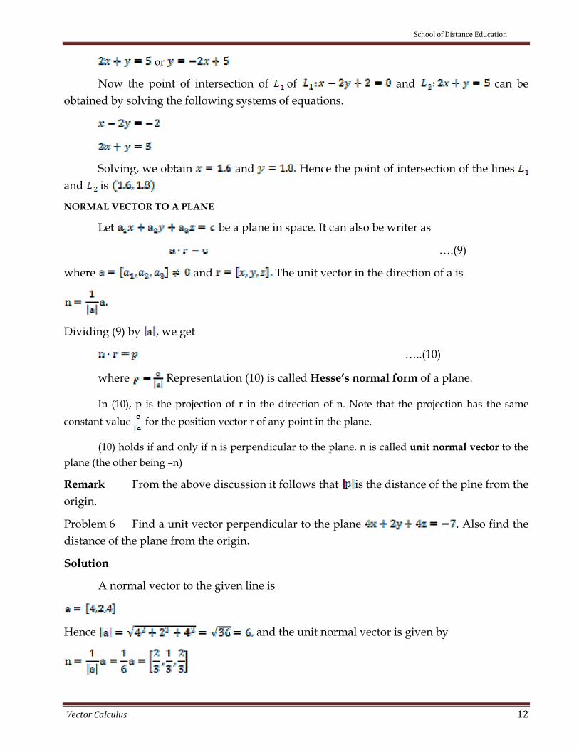
NORMAL VECTOR TO A PLANE
Let be a plane in space. It can also be writer as
….(9)
where and The unit vector in the direction of a is
Dividing (9) by , we get
…..(10)
where Representation (10) is called Hesse’s normal form of a plane.
In (10), p is the projection of r in the direction of n. Note that the projection has the same
constant value for the position vector r of any point in the plane.
(10) holds if and only if n is perpendicular to the plane. n is called unit normal vector to the plane (the other being –n)
Remark From the above discussion it follows that is the distance of the plne from the origin.
Problem 6 Find a unit vector perpendicular to the plane . Also find the distance of the plane from the origin.
Solution
A normal vector to the given line is
Hence and the unit normal vector is given by
School of Distance Education
Vector Calculus 13
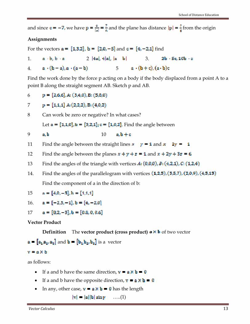
and since we have and the plane has distance from the origin
Assignments
For the vectors , and find
1. , 2 , , 3.
4. 5
Find the work done by the force p acting on a body if the body displaced from a point A to a point B along the straight segment AB. Sketch p and AB.
6
7
8 Can work be zero or negative? In what cases?
Let . Find the angle between
9 10
11 Find the angle between the straight lines and
12 Find the angle between the planes and
13 Find the angles of the triangle with vertices
14. Find the angles of the parallelogram with vertices
Find the component of a in the direction of b:
15
16.
17
Vector Product
Definition The vector product (cross product) of two vector
and is a vector
as follows:
• If a and b have the same direction,
• If a and b have the opposite direction,
• In any, other case, has the length …..(1)

School of Distance Education
Vector Calculus 14
where is the angle between a and b. This is the area of the parallelogram with a and b as adjacent sides The direction of is perpendicular to both a and b and such that a,b,v in this order, form a right handed triple.
CROSED PRODUCT IN COMPONENTS
In components, the cross product is given by
….(2)
Notice that in (2)
Hence is the expansion of the determinant
by the first row.
Definition A Cartesian coordinate system is called right-handed if the corresponding unit vectors I,j,k in the positive directions of the axes form a right handed triple. The system is called left-handed if the sense of k is reversed.
Problem Find the vector product of and in right-handed coordinates.
Solution
or
Problem With respect to a right-handed Cartesian coordinate system, let and Then
Vectors Product and Standard basis vectors
Since i,j,k are orthogonal (mutually perpendicular) unit vectors, the definition of vector product gives some useful formulas for simplifying vector products; in right-handed

School of Distance Education
Vector Calculus 15
coordinates these are
…… (3)
For left-handed coordinates, replace k by –k , Thus
GENERAL PROPERTIES OF VECTOR PRODUCT
Cross multiplication has the following properties:
• For every scalar l …(4)
• It is distributive with respect to vector addition, that is, (a)
(b) ….(5)
• Vector product is not commutative but anticommutative, that is, …(6)
• It is not associative, that is in general
so that the parentheses cannot be omitted.
Proof.
(4) follows directly from the definition.
…(8)
The sum of the two determinants in (8) is the first component of the right side of (5a). For the other components in (5a) and in (5b), equality follows by the same idea.
Now to get (6), note that
, using (2**)
, as the interchange of rows 2
And 3 multiples the determinants by -1
again using (2**)

School of Distance Education
Vector Calculus 16
We can confirm this geometrically if we set and then by (11) and for b, a,w to from a right handed triple, we must have
For the proof of (7), note that
, where as
SCALAR TRIPLE PRODUCT
Definition (Scalar Triple Product) The scalar product of three vectors a,b and c, denoted by , is defined as :
The scalar triple product is also denoted by and is also called the box product of the three vectors
Remarks
• The scalar triple product is a scalar quantity.
• Since the scalar triple product involves both the signs of ‘cross’ and ‘dot’ it is some times called the mixed product.
Geometrical meaning of Scalar triple product
The scalar triple product has a geometrical interpretation. Consider the parallelepiped with a, b and c as co terminus edges. Its height is the length of the component of a on . To be precise, we should say that this height is the magnitude of
, where is the angle between a and .
Now,
Where the sign or depends on which is positive or negative according is acute or obtuse that is according as a, b, c is right handed or left handed.
Hence the volume of the parallelepiped with co terminal edges a, b and c is , up to sign, the scalar triple product.
Expression for the scalar triple product as a determinant
Let and
Then the scalar triple product can be easily evaluated using the following formula:

School of Distance Education
Vector Calculus 17
Problem Compute if and
Solution
Problem Find the volume of the parallelepiped whose co-terminal edges are arrows representing the vectors and
Solution
Problem Find the volume of the tetrahedron with co terminal edges representing the vectors and
Solution
The volume of the tetrahedron
Hence, the volume of the tetrahedron is
Theorem (Linear independence of three vectors) Three vectors form a linearly independent set if and only if their scalar triple product is not zero.
The following is restatement of the above Theorem.
Theorem Scalar triple product of three coplanar vectors is zero.
Proof. Let be three coplanar vectors. Now represent a vector which is perpendicular to the plane containing b and c in which also lies the vector a and hence is perpendicular to a. Therefore Thus when three vectors are coplanar.

School of Distance Education
Vector Calculus 18
Conversely, suppose that . That is , which shows that is perpendicular to a. But is vector perpendicular to the plane containing b and c hence a should also lie in the plane of b and c. That is a, b, c are coplanar vectors.
Problem 11 Show that the vectors are linearly independent.
Solution
By the Theorem, it is enough to show that the scalar triple product of the given vectors is not zero. It can be seen that the scalar triple product is not zero. Hence the given vectors are linearly independent.
Problem Find the constant so that the vectors are coplanar.
Solution Three vectors a, b, c are coplanar if
i.e, if or if or if
Problem Prove that the points and are coplanar.
Solution
Let the given points be respectively and if these four points are coplanar then the vectors are coplanar, so that their scalar triple product is zero. i.e
Now sition vector of position vector of
Similarly
Now
Hence the given points are coplanar.
Equation of a Plane with three points
Let
and c=x3i+y3j+z3k be the position vectors of three points and
Let us assume that the three points and do not lie in the same straight line. Hence they determine a plane. Let be the position vector of any point

School of Distance Education
Vector Calculus 19
in the plane. Consider the vectors which all lie in the plane. That is and are coplanar vectors. Now we apply the condition for coplanar vectors.
or
or
Problem Find the equation for the plane determine by the points and
Solution
The equation of a plane with three points and is given by
Hence here, the equation of the plane with the points and is given by
or
i.e, the equation of the plane is
or
Assignments
In Assignments 1-9 with respect to a right-handed Cartesian coordinate system, let Find the following expressions.
1. 2.
3 4 .
5 6
7 8
9

School of Distance Education
Vector Calculus 20
10 What properties of cross multiplication do Assignments 1,4 and 5 illustrate ?
11 A wheel is rotating about the x-axis with angular speed 3 The rotation appears clockwise if one looks from the origin in the positive x-direction. Find the velocity and the speed at the point .
12 What are the velocity and speed in Exercise 11 at the point if the wheel rotates about the y-axis and ?
A force p acts on a line through a point A. Find the moment vector m of p about a point are
13
14
15 Find the area of the parallelogram if the vertices are
16 Find the area of the triangle in space if the vertices are
17 Find the plane through
18 Find the volume of the parallelepiped if the edge vectors are
19 Find the volume of the tetrahedron with the vertices
20 Are the vectors linearly independent ?
LINES AND PLANES IN SPACE
In this chapter we show how to use scalar and vector products to write equations for lines, line segments, and planes in space.
Lines and Line Segments in Space
Suppose is line in space passing through a point and is parallel to a vector Then is the set of all points for which is parallel to v. That
is, lies on if and only if is a scalar multiple of .
Vector equation for the line through and parallel to v is given by
…(1)
Expanding Eq. (1), we obtain
Equating the corresponding components of the two sides gives three scalar equations involving the parameter t:

School of Distance Education
Vector Calculus 21
When rearranged, these equations give us the standard parameterization of the line for the interval as follows :
……(2)
Standard parameterization of the line through and parallel to is given by above.
Problem Find parametric equations for the line through and parallel to .
Solution
With equal to and equal to Eq (2) become
Problem Find parametric equations for the line through and .
Solution
The vector
is parallel to the line , and Eg.(2) with “base point” give
…..(3)
If we choose as the “base point” we obtain
…..(4)
The equations in (4) serve as well as the equations in (3); they simply place you at a different point for a given value of .
Line Segment Joining Two Points
To parameterize a line segment joining two points, we first parameterize the line through the points. We then find the values for the end points and restrict to lie in the closed interval bounded by these values. The line equations together with this added restriction parameterize the segment.
Problem Parameterize the line segment joining the points and .
Solution
We begin with equations for the line through and , which obtained in Problem 2:
…..(5)

School of Distance Education
Vector Calculus 22
We observe that the point
Passes through at and at We add the restriction to Eq (3) to parameterize the line segment:
…..(6)
The Distance from a Point to a Line in Space
To find the distance from a point to to a line that passes through a point parallel to a vector v, we find the length of the component of normal to the line . In the notation
of the figure, the length is which is
Distance from a Point to a Line Through parallel to is given by
......(7)
Problem Find the distance from the point to the line
......(8)
Solution
Putting we see from the equations for that passes through and is parallel to (v is obtained by comparing (8) with (2) to get With
and
Eq. (7) gives
Equations for planes in Space
Suppose plane passes through a point and is normal (perpendicular) to the nonzero vector Then is the set of all points for which
is orthogonal to
That is, lies on if and only if This equation is equivalent to
or

School of Distance Education
Vector Calculus 23
i.e. Plane Through normal to is given by the following equivalent equatations:
Vector equation : ….(9)
Component equatation :
….(10)
Problem Find an equatation for the plane through perpendicular to .
Solution
Using Eq. (10),
Problem Find the plane through
Solution
We find a vector normal to the plane and use it with one of the points (it does not matter which) to write an equatation for the plane.
The cross Product is normal to the plane. Note that Similiarly,
Hence
We substitute the components of this normal vector and the co ordinates of the point (0,0,1) into Eq. (10) to get
i.e
Problem Find the point where the line
Intersects the plane
Solution
The point

School of Distance Education
Vector Calculus 24
…(12)
Lies in the plane if its coordinates satisfy the equatation of the plane; that is, if
Putting the point of intersection is
The Distance from a Point to a Plane
ProblemFind the distance from to the plane
Solution
We follow the above algorithm.
Using (11) vector normal; to the given plane is given by
The poins on the plane easiest to find from the plane’s equation are the intercepts .If we take to be the y-intercept, then putting and in the equation of the plane or
Hence is , and then
The distance from to the plane is
Angles Between Planes; Lines of Intersection
The angle between two intersecting planes is defined to be the ?(acute) angle determined by their normalvectors

School of Distance Education
Vector Calculus 25
Problem Find the angle between the planes and
Solution
Using (11), it can be seen that the vectors
are normals to the given planes and respectively. The angle between them (using the definition of dot product) is
Problem Find the vector parallel to the line of intersection of the planes and .
Solution
The line of intersection of two planes is perpendicular to the plane’s normal vector’s and , and therefore parallel to .In particular is a vector parallel to the
plane’s line of intersection. In our case,
,
We note that any nonzero scalar multiple of is also a vector parallel to the line of intersection of the planes and .
Problem Find parametric equations for the line in which the planes and intersect.
Solution
v =14i+2j+15k as a vector parallel to the line. To find a point on the line, we can take any point common to the two planes. Substituting z=0 in the plane equations we obtain
and solving for the x and y simultaneously gives x=3, y= -1. Hence one of the point common to the plane is (3,-1,10)
The line is [Using eq.(2)]
Assignments
Find the parametric equations for the lines in Exercise 1-6

School of Distance Education
Vector Calculus 26
1. The line through the point parallel to the vector i+j+k 2. The line through and 3. The line through the origin parallel to the vector 2j+k 4. The line through (1,1,1) parallel to the z-axis 5. The line through perpendicular to the plane 6. The x-axis
Find the parametrizations for the line segments joining the points in Assignments 7-10. Draw coordinate axes anD sketch each segments indicating the direction of increasing t for your parametrization.
7. , 8. ,
9 , . 10 ,
Find equations for the planes in Assignments 11-13.
11. The plane through normal to
12 The plane through and
13 The plane through perpendicular to the line
14 Find the point of intersection of the lines
and
15 Find the plane determined by the intersection of the lines:
16 Find a plane through and perpendicular to the line of intersection of the planes
In Assignments 17-19, find the distance from the point to the line.
17
18
19
In Exercise 20-22 , find the distance from the point to the plane.
20
21

School of Distance Education
Vector Calculus 27
22
23 Find the distance from the plane to the plane,
24 Find the angles between the following planes:
Use a calculator to find the acute angles between planes in Assignments 25-26 to the nearest hundredth of a radial.
25.
26
In Exercise 27-28 , find the point in whixh the line meets the given planes
27
28.
Find parametrizations for the lines in which the planes in Assignments 29 intersect.
29.
30.
Given two lines in space, either they are parallel, or they intersect or they are skew (imagine, for Problem the flight paths of two planes in the sky). Exercise 31 give three lines. Determine whether the lines, taken two at a time, are parallel, intersect or are skew. If they interesect, find the point of intersection.
31
CYLINDERS,SPHERE,CONE AND QUADRIC SURFACES
Definition A cylinder is a surface generated by a line which is always parallel to a fixed line passes through (intersects) a given curve.
The fixed line is called the axis of the cylinder and the given curve is called a guiding curve or generating curve
Remark
• If the guiding curve is a circle, the cylinder is called a right circular cylinder.
• Since the generator is a straight line, it extends on either side infinitely. As such , a cylinder is an infinite surface.

School of Distance Education
Vector Calculus 28
• The degree of the equation of a cylinder depends on the degree of the equation of the guiding curve.
• A cylinder, whose equation is of second degree, is called a quadric cylinder.
When graphing a cylinder or other surface by hand or analyzing one generated by a computer, it helps to look at the curves formed by intersecting the surface with planes parallel to the coordinate planes. These curves are called cross sections or traces.
We now consider a cylinder generated by a parabola.
Problem Find an equation for the cylinder made by the lines parallel to the z-axis that pass through the parabola
Solution
Suppose that the point lies on the parabola in the plane. Then, for any value of z, the point will lie on the cylinder because it lies on the line
through parallel to the z-axis. Conversely any point whose y-coordinate is the squre of it x-coordinate lie on the cylinder because it lies on the line
through parallel to the z-axis
Remark Regardless of the value of z, therefore, the points on the surface are the points whose coordinates satisfy the equation . This makes an equation for the cylinder. Because of this, we call the cylinder “the cylinder ’’.
As Problem 1 or the Remark follows it suggests, any curve in the - plane defines a cylinder parallel to the z-axis whose equation is also
Problem The equation defines the circular cylinder made by the lines parallel to the z-axis that pass through the circle in the xy-plane.
School of Distance Education
Vector Calculus 29
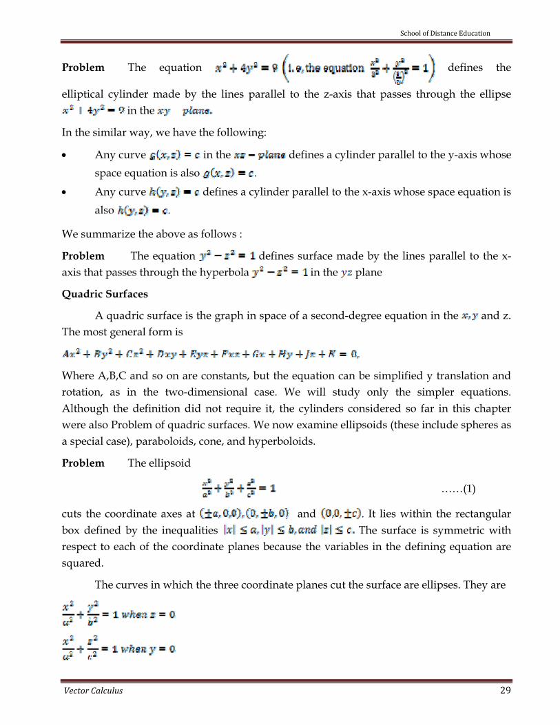
Problem The equation defines the
elliptical cylinder made by the lines parallel to the z-axis that passes through the ellipse in the
In the similar way, we have the following:
• Any curve in the defines a cylinder parallel to the y-axis whose space equation is also .
• Any curve defines a cylinder parallel to the x-axis whose space equation is also .
We summarize the above as follows :
Problem The equation defines surface made by the lines parallel to the x-axis that passes through the hyperbola in the plane
Quadric Surfaces
A quadric surface is the graph in space of a second-degree equation in the and z. The most general form is
Where A,B,C and so on are constants, but the equation can be simplified y translation and rotation, as in the two-dimensional case. We will study only the simpler equations. Although the definition did not require it, the cylinders considered so far in this chapter were also Problem of quadric surfaces. We now examine ellipsoids (these include spheres as a special case), paraboloids, cone, and hyperboloids.
Problem The ellipsoid
……(1)
cuts the coordinate axes at and . It lies within the rectangular box defined by the inequalities The surface is symmetric with respect to each of the coordinate planes because the variables in the defining equation are squared.
The curves in which the three coordinate planes cut the surface are ellipses. They are

School of Distance Education
Vector Calculus 30
The section cut from the surface by the plane is the ellipse
…..(2)
Special Cases: If any two of the semi axes a, b and c are equal, the surface is an ellipsoid of revolution. If all three are equal, the surface is sphere.
Problem The elliptic paraboloid
…..(3)
is symmetric with respect to the planes and as the variables x and y in the defining equation are squared. The only intercept on the axes is the origin (0,0,0). Except for this point, the surface lies above or entirely below the xy-plane, depending on the sign of c. The sections cut by the coordinate planes are
…..(4)
Each plane above the xy-plane cuts the surface in the ellipse
Problem The circular paraboloid or paraboloid of revolution
…..(5)
is obtained by taking by b=a in Eg. (3) for the elliptic paraboloid. The cross sections of the surface by planes perpendicular to the z-axis are circles centered on the z-axis. The cross sections by planes containing the z-axis are congruent parabolas with a common focus at the point (0,0, .
Application : Shapes cut from circular paraboloids are used for antennas in radio telescopes, satellite trackers, and microwave radio links.
Definition A cone is a surface generated by lines all of which pass through a fixed point (called vertex) and
(i) all the lines intersect a given curve (called guiding curve)
or (ii) all the lines touch a given surface

School of Distance Education
Vector Calculus 31
or (iii) all the lines are equally inclined to a fixed line through the fixed point.
The moving lines which generate a cone are known as its generators. When the moving lines satisfy condition (ii) in the definition of a cone, we term the cone as enveloping cone.
Problem The elliptic cone
…..(6)
is symmetric with respect to the three coordinate planes Fig (7). The sections cut by coordinate planes are
…(7)
……(8)
The secions cut by planes above and below the xy-plane are ellipse whose enters lie on the z-axis and whose vertices lie on the lines in Eq.(7) and (8).
If a=b, the cone is a right circular cone.
Problem 9 The hyperboloid of one sheet
….(9)
is symmetric with respect to each of the three coordinate planes . The sections cut out by the coordinate planes are
…..(10)
The plane cuts the surface in an ellipse with center on the z-axis and vertices on one of the hyperbolas in (10)
If a=b, the hyperboloid is a surface of revolution
Remark : The surface in Problem 9 is connected, meaning that it is possible to travel from one point on it to any other without leaving the surface. For this reason it is said to have one sheet, in contrast to the hyperboloid in the next Problem, which as two sheets.
Problem The hyperboloid of two sheets
….(11)

School of Distance Education
Vector Calculus 32
is symmetric with respect to the three coordinate planes. The plane z=0 does not intersect the surface; in fact, for a horizontal plane to intersect the surface, we must have The hyperbolic sections
have their vertices and foci on the . The surface is separated into two portions, one above the plane and the other below the plane . This accounts for the name, hyperboloid of two sheets.
Eq.(9) and (11) have different numbers of negative terms. The number in each case is the same as the number of sheets of the hyperboloid. If we replace the I on the right side of either Eq.(9) or Eq.(11) by 0, we obtain the equation
for an elliptic cone (Eq.6). The hyperboloids are asymptotic to this cone in the same way that the hyperbolas
are asymptotic to the lines
In the xy-plane.
Problem The hyperbolic paraboloid
…..(12)
Has symmetry with respect to the planes and . The sections in these planes are
………. (13)
….(14)
In the plane x=0, the parabola opens upward from the origin. The parabola in the plane y=0 opens downward.
If we cut the surfaces by a plane , the section is a hyperbola.
……(15)
With its focal axis parallel to the y-axis and its vertices on the parabola in (13).

School of Distance Education
Vector Calculus 33
If is negative, the focal axis is parallel to the x-axis and the vertices lie on the parabola in (14).
Near the origin, the surface is shaped like a saddle. To a person travelling along the surface in the yz-plane, the origin looks like a minimum. To a person travelling along the surface in the xz-plane, the origin looks like a maximum. Such a point is called a minimax or saddle point of surface.
Assignments
Sketch the surfaces in Assignments 1-32
1. 2.
3 . 4
5. 6
7. 8.
9.
10. 11.
12. 13.
14. 15.
16.
17 18.
19 20.
21 22.
23. 24.
25. 26.
27. 28.
29. 30.
31. 32
CYLINDRICAL AND SPHERICAL COORDINATES
Cylindrical and Spherical Coordinates
This section introduces two new coordinate systems for space: the cylindrical coordinate system and the spherical coordinate system. Cylindrical coordinates

School of Distance Education
Vector Calculus 34
simplify the equations of cylinders. Spherical coordinates simplify the equations of spheres and cones.
Cylindrical Coordinates
We obtain cylindrical coordinates for space by combining polar coordinates in the xy-plane with the usual z-axis. This assigns to every point in space one or more coordinates triples of the form (r, θ, z), as shown in Fig 1.
Definition
Cylindrical coordinates represent a point P in space by ordered triples (r, θ , z) in which
1. r and θ are polar coordinates for the vertical projection of P on the xy - plane,
2. z is the rectangular vertical coordinate.
The values of x, y, r , and θ in rectangular and cylindrical coordinates are related by the usual equations.
Equations Relating Rectangular (x,y,z) and Cylindrical (r, θ, z) Co ordinates x = r cos θ, y = r sin θ, z = z ; r2 = x2 + y2 tan θ =
In cylindrical coordinates , the equation r = a describes not just a circle in the xy-plane but an entire cylinder about the z-axis . The z-axis is given by r = 0. The equation θ= θ0 describes the plane that contains the z- axis and makes an angle θ0 with the positive x-axis. And, just as in rectangular coordinates, the equation z= z0 describes a plane perpendicular to the z-axis.
Problem What points satisfy the equations
r = 2, θ =
Solution These points make up the line in which the cylinder r = 2 cuts the portion of the plane θ = where r is positive. This is the line through the point (2, , 0)parallel to the z -axis.
Along this line, z varies while r and θ have the constant values r = 2 and θ =
Problem Sketch the surface r = 1 + cos θ
Solution The equation involves only r and θ; the coordinate variable z is missing . Therefore, the surface is a cylinder of lines that pass through the cardioid r = 1 + cos θ in the r θ-plane and lie parallel to the z-axis. The rules for sketching the cylinder are the same as always: sketch the x-, y-, and z-axes, draw a few
(1)

School of Distance Education
Vector Calculus 35
perpendicular cross sections, connect the cross sections with parallel lines , and darken the exposed parts.
Problem Find a Cartesian equation for the surface z = r2 and identity the surface.
Solution From Eqs. (1) we have z=r2 = x2 + y2. The surface is the circular paraboloid x2 + y2 = z
Problem Find an equation for the circular cylinder 4x2 + 4y2 = 9 in cylindrical coordinates.
Solution The cylinder consists of the points whose distance from the z-axis is = The corresponding equation in cylindrical coordinates is
r =
Problems Find an equation for the cylinder x2 + (y−3)2 = 9 in cylindrical coordinates
Solution The equation for the cylinder in cylindrical coordinates is the same as the
polar equation for the cylinder's base in the xy- plane:
Spherical Coordinates
Definition Spherical coordinates represent a point P in space by ordered triples
( , in which
1. is the distance from P to the origin.
2. is the angle makes with the positive z-axis (0 ),
3. is the angle from cylindrical coordinates.
The equation = a describes the sphere of radius a centered at the origin. The equation
= 0 describes a single cone whose vertex lies at the origin and whose axis lies along the z-axis. (We broaden our interpretation to include the xy-plane as the cone ) If 0 is greater than , the cone = 0 opens downward.
Equations Relating Spherical Coordinates to Cartesian and Cylindrical Coordinates
r = , x = r cos = ,
r = , y = r sin = , (2)
Problem Find a spherical coordinate equation for the sphere
Solution We use Eqs. (2) to substitute for x, y and z:

School of Distance Education
Vector Calculus 36
1
1
Problem Find a spherical coordinate equation for the cone z =
Solution Use geometry. The cone is symmetric with respect to the z-axis and cuts the first quadrant of the yz-plane along the line z = y. The angle between the cone and the positive z-axis is therefore radians. The cone consists of the points whose spherical coordinates have equal to so its equations is
Assignments
In Assignments 1-26, translate the equations and inequalities from the given coordinates system (rectangular, cylindrical, spherical ) into equations and inequalities in the other two systems. Also , identify the figure being defined.
1. r = 0 2.
3. z = 0 4. z = −2
5. z = 6. z =
7. 8. = 1
9. 10.
11. = 5 cos 12. = −6 cos
13. r = csc θ 14. r = −3 sec θ
15. 16.
17.
18.
19.
20.

School of Distance Education
Vector Calculus 37
21. z = 4−4 , 0
22. z = 4−r, 0
23. , 0
24. , 0
25. z + = 0
26.
27. Find the rectangular coordinates of the center of the sphere
___________________________________
VECTOR- VALUED FUNCTIONS
AND SPACE CURVES
Space Curves
In this chapter, we shall consider the equations of the form
…..(1)
where, and are real valued functions of the scalar variable t. As t increases from its
initial value to the value the point trace out some geometric object in space;
it may be straight line or curve. This geometric object is called space curve or arc. Simply, the
equations
represent a curve in space. A space curve is the locus of the point whose co‐ordinates are
functions of a single variable
Definitions
When a particle moves through space during a time interval I, then the particle’s coordinates
can be considered as functions defined on I.
The points make up the curve in space that we call the particle’s
path. The equations and interval in (1) parameterize the curve.
The vector

School of Distance Education
Vector Calculus 38
from the origin to the particle’s position at time is the particle’s position
vector. The functions and h are the component functions (components) of the position vector.
We think of the particle’s path as the curve traced by during the time interval
Equation (1) defines as a vector function of the real variable on the interval More
generally, a vector function or vector‐valued function on a domain set D is a rule that assigns a
vector in space to each element in D. For now the domains will be intervals of real numbers. There
are situations when the domains will be regions in the plane or in space. Vector functions will then
be called “vector fields”. A detailed study on this will be done in later chapter.
We refer to real‐valued functions as scalar functions to distinguish them from vector
functions. The components of r are scalar functions of t. When we define a vector‐valued function
by giving its component functions, we assume the vector function’s domain to be the common
domain of the components.
Problem Consider the circle It is most convenient to use the
trigonometric functions with t interpreted as the angle that varies from . Then we
have
In this chapter we show that curves in space constitute a major field of applications of vector
calculus. To track a particle moving in space, we run a vector r from the origin to the particle and
study the changes in r.
Problem A straight line L through a point A with position vector in the
direction of constant vector can be represented in the form
……(2)
If b is a unit vector, its components are the direction cosines of L. In this case measures the
distance of the points of L from A.
Problem The vector function
is defined for all real values of t. The curve traced by r is a helix (from an old Greek word for “spiral”)
that winds around the circular cylinder . The curve lies on the cylinder because
the i‐ and j‐ components of r, being the x‐ and y‐ coordinates of the tip of r, satisfy the cylinder’s
equation:
The curve rises as the k‐component increase. Each time increases by the curve
completes one turn around the cylinder. The equations
Parameterize the helix, the interval being understood.

School of Distance Education
Vector Calculus 39
Limits
The way we define limits of vector‐valued functions is similar to the way we define limits of real‐
valued functions.
Definition
Let be a vector function and a vector. We say that has limit as
approaches and write
If, for every number , there exists a corresponding number such that for all
If , then precisely when
The equation
provides a practical way to calculate limits of vector functions.
Problem If then
and
We define continuity for vector functions the same way we define continuity for scalar functions.
Continuity
Definition A vector function is continuous at a point in its domain if
. The function is continuous if it is continuous at every point in its domain.
Component Test for Continuity at a Point
Since limits can be expressed in terms of components, we can test vector functions for continuity by
examining their components. The vector function is continuous at
if and only if the component functions are continuous at

School of Distance Education
Vector Calculus 40
Problem The function is contitinuous because the components
,cost,sint and t are continuous
Consider the function
is discontinuous at every integer. We note that the components and are continuous everywhere. But the function is discontinuous at every integer Hence is discontinuous at every integer.
Derivatives and Motion
Suppose that is the position vetor of a particles moving along a curve
in space and that are differentiable functions of Then the difference between the
particle’s positions at time and time is
In terms of components,
As approaches zero, three things seem to happen simultaneously.
• First, approaches along the curve.
• Second, the secant line seems to approach a limiting position tangent to the curve at
• Third, the quotient approaches the following limit
We are therefore led by past experience to the following definitions.
Definitions The vector function is differentiable at
.Also, is said to be differentiable if it is differentiable at
every point of its domain. At any point at which is differentiable, its derivative is the vector

School of Distance Education
Vector Calculus 41
Problem If find
Solution
Given Hence
Definition The curve traced by is smooth if is continuous and never 0, i.e., if
have continuous first derivatives that are not simultaneously 0.
Remark The vector when different from0, is also a vector tangent to the curve.
Definition The tangent line to the curve at a point is defined to be the line
through the point parallel to at .
Remark We require for a smooth curve to make sure the curve has a continuously
turning tangent at each point. On a smooth curve there are no sharp corners of cusps.
Definition A curve that is made up of a finite number of smooth curves pieced together in a
continuous fashion is called piecewise smooth
Definitions If r is the position vector of a particle moving along smooth curve in space, then
is the particle’s velocity vector, tangent to the curve. At any time the direction of is the
direction of motion, the magnitude of v is the particle’s speed, and the derivative when
it exists, is the particle’s acceleration vector. In short,
1. Velocity is the derivative of position :
2 Speed is the magnitude of velocity : Speed=
3 Acceleration is the derivative of velocity :
4 The vector is the direction of motion at time .
We can express the velocity of a moving particle as the product of its speed and direction.
Problem The vector

School of Distance Education
Vector Calculus 42
gives the position of a moving body at time . Find the body’s speed and acceleration when At
times, if any, are the body’s velocity and acceleration orthogonal ?
Solution
At , the body’s speed and direction are
Speed :
Direction
To find the times when and are orthogonal, we look for values of for which
The only value is
Problem 8 A particle moves along the curve
Find the velocity and acceleration at
Solution
Here the position vector of the particle at time is given by
Then the velocity is given by
and the acceleration a is given by
When , and
Problem Show that if b, c, d are constant vectors, then
is a path of a point moving with constant acceleration.
Solution
The velocity v is given by

School of Distance Education
Vector Calculus 43
since the derivative of the constant vector d is 0
The acceleration a is given by
The above is a constant vector, being a scalar multiple of the constant vector b. Hence the result.
Problem A particle moves so that its position vector is given by
where is a constant. Show that
(i) the velocity of the particle is perpendicular to r (ii) the acceleration is directed towards the origin and has magnitude proportional to the
distance from the origin.
(iii) is a constant vector.
Solution
(i) The velocity v is given by
Now
Hence velocity of the particles is perpendicular to r.
(ii) The acceleration a is given by
Thus direction of acceleration is opposite to that vector r and as such
it is directed towards the origin and the magnitude is proportional
to . i.e., the acceleration is directed towards the origin and has magnitude
proportional to the distance from the origin
(iii)
a constant vector.

School of Distance Education
Vector Calculus 44
Problem (Centripetal acceleration) suppose a particle moves along a circle C having radius R in
the counter clock wise sense. Then its motion is given by the vector function
…. (1)
The velocity vector
Is a tangent at each point to the circle C and it magnitude
is constant, Hence
so that is the called the angular speed.
The acceleration vector is
with magnitude . Since are constants this implies that there is an
acceleration of constant magnitude towards the origin.( due to negative sign). This acceleration
is called centripetal acceleration. It results from the fact that the velocity vector is changing
direction at a constant rate. The centripetal force is Where is the mass of . The opposite
vector is called centrifugal force, and the two forces are in equilibrium at each instant of the
motion.
Differentiation Rules
Because the derivatives of vector functions may be computed component by component,
the rules for differentiating vector functions have the same form as the rules for differentiating
scalar functions They are :
Constant Function Rule : (any constant vector C)
If and are differentiable vector functions of t, then
Scalar Multiple Rules : (any number C)
(any differentiable scalar function f(t))
Sum Rule :
Difference Rule :
Dot Product Rule :

School of Distance Education
Vector Calculus 45
Cross product rule
Chain Rule (Short Form) : If r is a differentiable function of t and t is a differentiable function of s, then
We will prove the dot and cross product rules and Chain Rule and leaving the others as Assignments .
Proof of the Dot Product Rule Suppose that
and
Then
u'.v u.v’
Proof of the Cross Product Rule
According to the definition of derivative,
To change this fraction into an equivalent one that contains the difference quotients for the derivates of u
and v, we subtract and add in the numerator. Then
The last of these equalities holds because the limit of the cross product of two vector functions is
the cross product of their limits if the latter exist. As approaches zero, approaches
because v, being differentiable at is continuous at The two fractions approach the values of
and at In short

School of Distance Education
Vector Calculus 46
Proof the Chain Rule Suppose that is a differentiable vector function of
and that t is a differentiable scalar functions of some other variable . Then are differentiable
functions of and the Chain Rule for differentiable real‐valued functions gives
Problem Show that
Solution
Let then
and
Also
or
Constant Vectors
A vector changes if either its magnitude changes or its direction changes or both direction and
magnitude change.
Theorem A The necessary and sufficient condition for the vector function to be constant is
that the zero vector,
Solution
Necessary Part If is constant, then .
Hence

School of Distance Education
Vector Calculus 47
Sufficiency Part Conversely, suppose that
Let
Then
Hence using the assumption we have
Equating the coefficients, we get
and this implies that and are constants, (in other words this means that
and are independent of .
Therefore is a constant vector.
Theorem B The necessary and sufficient condition for the vector function to have constant
magnitude is that
Solution Let F be a vector function of the scalar variable
Suppose to have constant magnitude, say F, so that Then
Therefore,
or or or
Conversely, suppose that . Then
or or or
and this implies that is a constant or is a constant. i.e. the vector function have constant
magnitude.
Theorem C The necessary and sufficient condition for the vector function to have constant
direction is that
Solution
Let be a vector function of the scalar variable and n be a unit vector in the direction of If be
the magnitude of then

School of Distance Education
Vector Calculus 48
(since
by theorem B)
…….(1)
Necessary Part Suppose that F has constant direction. Then n is a constant vector. Therefore,
. Hence by (1) above we have
Sufficiency Part
Conversely, suppose that . Then from (1), we get
or ….(2)
Since n is of constant length, by the last theorem, we have
…(3)
From (2) and (3), we obtain . Hence n is a constant vector. Therefore the direction of F is
constant.
Vector Functions of a Constant Length
When we track a particle moving on a sphere centered at the origin the position vector has a
constant length equal to the radius of the sphere. The velocity vector , tangent to the path of
motion, is tangent to the sphere and hence perpendicular to r, This is always the case for a
differentiable vector function of constant length (as seen in Theorem above): The vector and its first
derivative are orthogonal. With the length constant, the change in the function is a change in
direction only, and direct changes take place at the right angles.
If is differentiable vector functions of of constant length, then
…..(3)
For the proof of (3) see Theorem above.
Problem Show that

School of Distance Education
Vector Calculus 49
has constant length and is orthogonal to its derivative.
Solution
Integrals of Vector Functions
A differentiable vector function is an anti derivative of a vector function on an interval if
at each point of If is an anti derivative of on it can be shown, working one
component at a time, that every anti derivative of on has the form of for some constant
vector . The set of all anti derivates of on is the indefinite integral on
Definition The indefinite integral or with respect to is the set of all anti derivatives of ,
denoted by If is any anti derivative of then
The usual arithmetic rules for indefinite integrals apply.
Problem
…… (4)
……(5)
with
As in the integration of scalar functions, it is recommended that you skip the steps in (4) and (5) and
go directly to the final form. Find an anti derivative for each component and add a constant vector
at the end.
Problem 15 Evaluate where A is a vector function in the variable
Solution We know that
Hence

School of Distance Education
Vector Calculus 50
where is an arbitrary constant vector.
Problem Prove that
Solution We know that
Differentiating with respect to on both sides, we get
On integration, we get
Definite integrals
Definite integrals of vector functions are defined in terms components.
Definition
If the component of are integral over then so is r, and the
definite integral of from to is
The usual arithmetic rules for definite integrals apply.
Problem If find
Solution

School of Distance Education
Vector Calculus 51
Where is an arbitrary constant vector
(ii)
Problem
Problem The velocity of a particle moving in space is
Find the particle’s position as a function of if when
Solution
Our goal is to solve the initial value problem that consists of
The differential equation :
The initial condition :
Integrating both sides of the differential equation with respect to gives
We then use the initial condition to find the right value for C :
implies
The particle’s position as a function of t is
To check (always a good idea), we can see this formula that
and =2i+k

School of Distance Education
Vector Calculus 52
Problem The acceleration of a particle at time is given by If
the velocity and the displacement be zero at Find and at time
Solution Given
On integration,
Putting when we get
so that hence
(ii) Since we have
Integrating we get
Putting when we get
So that hence
Assignments
Assignments 1‐2, r(t) is the position of a particle in the xy‐plane at time t. Find an equation in x and
y whose graph is the path of the particle. Then find the particle’s velocity and acceleration vectors at
the given value of t.
1.
2.
Assignments 3‐4 give the position vectors of particles moving along various curves in the xy‐plane.
In each case, find the particles velocity and acceleration vectors at the stated times and sketch them
as vectors in the curve

School of Distance Education
Vector Calculus 53
3. (Motion on the circle)
and
4 (Motion on the cycloid)
and
In Assignments 5‐7, r(t) is the position of particles in space at time r(t) Find the particle’s velocity
and acceleration vectors. Then find the particles speed and direction of motion at the given value of
t. Write the particles velocity at the time as the product of its speed a nd direction.
5.
6
7
In Assignments 8‐10 r(t) is the position of a particle in space at time t. and the angle between the
velocity and acceleration vectors at time t=0.
8
9
10 The position vector of a particle in space at time is given by
. Find the time or times in the given time
interval when the velocity and acceleration vectors are orthogonal.
Evaluate the integrals in Assignments 11‐13.
11
12
13
Solve the initial value problems in Assignments 14‐16 for r a vector function of t.
14 Differential equation :
Initial condition :
15 Differential equation :
Initial condition :
16 Differential equation :

School of Distance Education
Vector Calculus 54
Initial condition : and
The tangent line to smooth curve at is the line that passes through the
point parallel to , the curve’s velocity vector at . IN Assignments 17‐18,
find parametric equations for the line that is tangent to the given curve at the given parameter
value .
17
18
19 Each of the following equations (a)‐(e) describes the motion of a particle having the same
path, namely the unit circle . Although the path of each particle in (a)‐(e) is the
same, the behavior, or “dynamics”, of each particle is different. For each particle, answer the
following questions.
i) Does the particle have constant speed? If so, what is its constant speed?
ii) Is the particle’s acceleration vector always orthogonal to its velocity vector ?
iii) Does the particle move clockwise or counter clockwise around the circle ?
iv) Does the particle begin at the point (1,0) ?
a)
b)
c) .
d) .
e)
20 At time t=0, a particle is located at the point (1,2,3). It travels in a straight line to the point
(4,1,4), has speed 2 at (1,2,3) and constant acceleration 3i‐j+k. Find an equation for the position
vector r(t) of the particle at time t
ARC LENGTH AND
THE UNIT TANGENT VECTOR T
Arc Length Along a Curve
One of the special features of smooth space curves is that they have a measurable length.
This enable us to locate points along these curves by giving their directed distance along the curve
from some base point, the way we locate points on coordinate axes by giving their directed distance
from the origin Time is the natural parameter for describing a moving body’s velocity and
acceleration, but is the natural parameter for studying a curve’s shape. Both parameters appear in
analyses of space flight.

School of Distance Education
Vector Calculus 55
To measure distance along a smooth curve in space, we add a z‐term to the formula we use
for curves in the plane.
Definition
The length of a smooth curve , that is traced exactly
once as increases from is
……….(1)
We usually take then
…..(2)
Just as for plane curves, we can calculate the length of a curve in space from any convenient
parameterization that meets the stated conditions. The square root in either or both of Eqs.(1) and
(2) is the length of the velocity vector . Hence we have the Length Formula (Short Form)
Problem Find the length of one turn of the helix
Solution
The helix makes one full turn as runs from
Using the length formula (short form), the length of this portion of this curve is
This is times the length of the circle in the plane over which the helix stands.
If we choose a base point on a smooth curve parameterized by each value of
determines a point on and a “directed distance”.
…(4)
measured along from the base point . If , is the distance from to . If
is the negative of the distance. Each value of determines a point on and this

School of Distance Education
Vector Calculus 56
parameterizes with respect to . We call an arc length parameter for the curve,. The parameter‘s
value increase in the direction of increasing .
Arc length parameter with base point is given by
……(5)
Problem If , the arc length parameter along the helix
from to is
Using Esq.(4)
Thus, and so on
Problem Show that if is a unit vector, then the directed distance along the line
From the point when is itself.
Solution
So (nothing that, being unit vector,
Speed on a Smooth Curve
Since the derivatives beneath the radical in Esq.(5) are continuous (the curve is smooth), the
Fundamental Theorem of Calculus tells us that is a differentiable function of with derivative
……....(6)
As we except, the speed with which the particle moves along its path is the magnitude of

School of Distance Education
Vector Calculus 57
Notice that while the base point plays a role in defining in Esq. (5) it plays no role in Esq.(6).
The rate at which a moving particle covers distance along its path has nothing to do with how far
away the base point is.
Notice also that since, by definition, is never zero for a smooth curve. We see once
again that is an increasing function of
The Unit Tangent Vector T
Since for the curves we are considering, is one‐to‐one and has an inverse that gives
as a differentiable function of The derivative of the inverse is
……(7)
This makes a differentiable function of whose derivative can be calculated with the Chain Rule to
be
………………..(8)
Equation (8) says that is a unit vector in the direction of v. We call the unit tangent
vector of the curve traces by and denote it by T.
Definition The unit tangent vector of a differentiable curve is
…….(9)
The unit tangent vector is a differentiable function of whenever is a differentiable function of
As we will see in the next chapter is one of three unit vectors in a travelling reference frame that
is used to describe the motion of space vehicle and other bodies moving in three dimensions.
Problem Find the unit tangent vector of the helix
Solution
Problem Find the unit tangent vector to the curve
At the point .

School of Distance Education
Vector Calculus 58
Solution The position vector of a point on the curve is given by
Then
Hence
Therefore,
Therefore at t=2, the unit tangent vector is
Problem Find the unit tangent vector at a point t to the curve
Solution
Problem Find the unit tangent vector of the curve
Solution
Definition The involute of a circle is the path traced by the endpoint of a string unwinding
from a circle. In the above Problem it is the unit circle in the plane.
Problem For the counterclockwise motion
around the unit circle,
is already a unit vector, so
School of Distance Education
Vector Calculus 59
Assignments
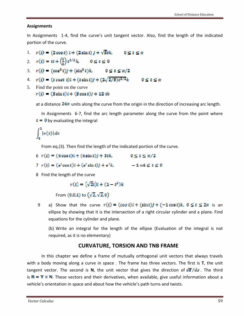
In Assignments 1‐4, find the curve’s unit tangent vector. Also, find the length of the indicated
portion of the curve.
1.
2.
3.
4.
5. Find the point on the curve
at a distance units along the curve from the origin in the direction of increasing arc length.
In Assignments 6‐7, find the arc length parameter along the curve from the point where
by evaluating the integral
From eq.(3). Then find the length of the indicated portion of the curve.
6
7
8 Find the length of the curve
From to
9 a) Show that the curve is an
ellipse by showing that it is the intersection of a right circular cylinder and a plane. Find
equations for the cylinder and plane.
(b) Write an integral for the length of the ellipse (Evaluation of the integral is not
required, as it is no elementary)
CURVATURE, TORSION AND TNB FRAME
In this chapter we define a frame of mutually orthogonal unit vectors that always travels
with a body moving along a curve in space . The frame has three vectors. The first is T, the unit
tangent vector. The second is N, the unit vector that gives the direction of . The third
is . These vectors and their derivatives, when available, give useful information about a
vehicle’s orientation in space and about how the vehicle’s path turns and twists.

School of Distance Education
Vector Calculus 60
For Problem, tells how much a vehicle’s path turn to the left or right as it moves
along; it is called the curvature of the vehicle’s path. The number .N tells how much a
vehicle’s path rotates or twists out of its plane of motion as the vehicle moves along; it is called the
torsion of the vehicle’s path. If is a train climbing up a curved track, the rate at which the
headlight turns from side to side per unit distance is the curvature of the track. The rate at which
the engine tends to twist out of the plane formed by T and N is the torsion.
Every moving body travels with a TNB frame that characterizes the geometry of its path
of motion.
The Curvature of a Plane Curve
As a particle moves along a smooth curve in the plane, turns as the curve bends. Since
T is an unit vector, its length remains constant and only its direction changes as the particle moves
along the curve. The rate at which T turns per unit of length along the curve is called the curvature .
The traditional symbol for the curvature function is the Greek letter (‘’Kappa”).
Definition
If T is the unit tangent vector of smooth curve, the curvature function of the curve is
If is large, T turns sharply as the particle passes through and the curvature at is large.
If is close to zero, T turns more slowly and the curvature at is smaller. Testing the
definition, we see in the following Problems 1and 2 that the curvature is constant for straight lines
and circles.
Problem (The curvature of a straight line is zero)
On a straight line, the unit tangent vector T always points in the same direction, so its components
are constants. Therefore .
Problem The parameterization for a circle having radius is
and substitute to parameterize in terms of arc length s. (Note that if the radius of the circle
and is the angle between two rays emanating from the centre, then the length of the arc of the
circle included between the rays is given by
Then

School of Distance Education
Vector Calculus 61
and
Hence, for any value of
The Principal Unit Normal Vector for Plane Curves
Since T has constant length, the vector is orthogonal to This conclusion is using the
result “If is a differentiable vector function of of constant length, then ’’
Therefore, if we divide by the length we obtain a unit vector orthogonal to T and
is given in the following definition.
Definition At a point where the principal unit normal vector for a curve in the plane is
The vector points in the direction in which T turns as the curve bends. Therefore, if
we face in the direction of increasing arc length, the vector points toward the right if T turns
clockwise and toward the left if T turns counter clockwise. In other words, the principal normal
vector N will point toward the concave side of the curve
Because the arc length parameter for a smooth curve is defined with
positive, and the Chain Rule gives
This formula enables us to find N without having to find and first.
Problem Find T and N for the circular motion

School of Distance Education
Vector Calculus 62
Solution We first find T:
From this we find
and
Circle of Curvature and Radius of Curvature
The circle of curvature or osculating circle at a point on a plane curve where is the circle in
the plane of the curve that
1. is tangent to the curve at ( has the same tangent line the curve has);
2. has the same curvature the curve has at and
3 lines toward the concave or inner side of the curve
The radius of curvature of the curve at is the radius of the circle of curvature, which
according to Problem 2 is
Radius of curvature=
To find , we find and take the reciprocal. The center of curvature of the curve at is the
center of the circle of curvature.
Curvature and Normal Vectors for Space Curves
Just as it for a curve in the plane, the arc length parameter gives the unit tangent vector
for a smooth curve in space. We again define the curvature to be
…..(3)
The vector is orthogonal to T and we define the principal unit normal to be
…….(4)
Problem Find the curvature for the helix

School of Distance Education
Vector Calculus 63
Solution We calculate T from the velocity vector v:
Then, using the Chain Rule, we find as
Chain Rule
nothing that so
Therefore
……(5)
From Eq. (5) we see that increasing for a fixed decreases the curvature. Decreasing for a fixed
eventually decreases the curvature as well .Stretching a spring teds to straighten it
if b=0 the Helix reduces to again as it should (we have seen earlier that the curvature of a straight
line is .
Problem Find for the helix in the previous Problem.
Solution
We have (using the previous Problem)

School of Distance Education
Vector Calculus 64
Torsion and the Binormal Vector
The Binormal Vector of a curve in space is a unit vector orthogonal to both and
. Together and define a moving right‐handed vector frame that plays a significant role in
calculating the flight paths of space vehicles.
How does behave in relation to and ? From the rule for differentiating a cross
product, we have
Since is the direction of , and
……(6)
From this we see that is orthogonal to since a cross product is orthogonal to its
factors.
Since is also orthogonal to (the latter has constant length), it follows that is
orthogonal to the plane of . In other words, is parallel to ,so is scalar
multiple of In symbols,
The minus sign in this equation is traditional. The scalar is called the torsion along the
curve. Notice that.
So that
Definition
Let . The torsion function of a smooth curve is
Unlike the curvature which is never negative, the torsion may be positive, negative or zero.
The curvature can be thought of as the rate at which the normal planes turns as the
point moves along the curve. Similarly, the torsion is the rate at which the
osculating plane turns about as moves along the curve. Torsion measures how the curve twists.

School of Distance Education
Vector Calculus 65
The Tangential and Normal Components of Acceleration
When a body is accelerated by gravity, brakes, a combination of rocket motors, or whatever, we
usually want to know how much of the acceleration acts to move the body straight ahead in the
direction of motion, in the tangential direction T. We can find out if we use the Chain Rule to rewrite
v as
and differentiable both ends of this string of equalities to get
……(7)
Where
……(8)
are the tangential and normal scalar components of acceleration.
Equation (7) is remarkable in that B does not appear. No matter how the path of the moving body
we are watching may appear to twist and turn in space, the acceleration a always lies in the plane of
T and N orthogonal to B. The equation also tells us exactly how much of the acceleration takes place
tangent to the motion and how much takes place normal to the motion
To calculate we usually use the formula , which comes from solving the
equation for . With this formula we can find without having to calculate
first.
…..(9)
Problem Without finding T and N, write the acceleration of the motion
in the form
Solution
We use the first of Eqs. (8) to find :

School of Distance Education
Vector Calculus 66
Knowing we use Eq.(9) to find
We then use Eq.(7) to find a:
Formulas for computing Curvature and Torsion
We now give some easy‐to‐use formulas for computing the curvature and torsion of a smooth
curve. From Eq.(7), we have
it follows that
A Vector Formula for Curvature
Solving for the discussion above gives the following vector formula for curvature
……(10)
Equation (10) calculates the curvature, a geometric property of the curve, from the velocity and
acceleration of any vector representation of the curve in which is different from zero. Take a
moment to think about how remarkable this really is : From any formula for motion along a curve,
no matter how variable the motion may be (as long as v is never zero), we can calculate a physical
property of the curve that seems to have nothing to do with the way the curve is traversed.
The most widely used formula for torsion is traversed.

School of Distance Education
Vector Calculus 67
…..(11)
Where and so on.
This formula calculate s the torsion directly from the derivates of the component functions
that make up The determinant’s first row comes from the
second row comes from and the third row come from .
Problem Use Eqs (10) and (11) to find and for the helix
Solution
We calculate the curvature with Eq.(10):
…….(12)
Notice that Eq.(12) agrees with Eq.(5) in an earlier Problem, where we calculate the curvature
directly from this its definition.
To evaluate Eq.(11) for the torsion, we find the entries in the determinant by differentiating with
respect to We already have and and
Hence,

School of Distance Education
Vector Calculus 68
………….(13)
*Formula for radius of curvature at a point on a curve in Cartesian co‐ordinates
The formula for radius of curvature at a point? on the curve. in the Cartesian co‐
ordinates is
where and
Problem Find the radius of curvature of at
Solution
Differentiating both sides of the given equation with respect to x,
……(1)
Differentiating (1), with respect to x, we obtain
at (3,4)
The centre of curvature is given by the formula
Problem Find the centre of curvature at the point to the curve . Solution

School of Distance Education
Vector Calculus 69
Given
which can be written as
Diffrentiating both sides with respect to we obtain
and
Hence at and
i.e., the centre of curvature at is .
Assignments
Find T,N and for the plane curves in Exercise 1‐2
1. 2.
In Exercise 3, write a in the form without finding T and N
3. 4. (A formula for the curvature of the graph of a function in the xy-plane)
(a) The graph in the xy plane automatically has the parameterization , and the vector formula Use this formula to show that if is a twice- differentiable function of then
(b) Use the formula for in (a) to find the curvature of . Compare your answer with the answer in Exercise 1.
5. (Normal’s to plane curves)
(a) Show that and , are both normal to the
curve , at the point .

School of Distance Education
Vector Calculus 70
To obtain N for a particular plane curve, we can choose the one of or from part (a) that
points toward the concave side of the curve, and make it into a unit vector. Apply this
method to find N for the following curves.
b)
c)
Find T, N, B, , and for the space curves in Exercise 6‐9.
6
7
8
9
10 Write a in the form without finding T and N, where
In Exercise 11‐12, write a in the form at the given value of t without finding
T and N
11.
12.
In Exercise 13, find r, T, N and B at the given value of t, Then find equations for the
osculating, normal, and rectifying planes at that value of t.
13

School of Distance Education
Vector Calculus 71
MODULE - II MULTIVARIABLE FUNCTIONS
AND PARTIAL DERIVATIVES
FUNCTIONS OF SEVERAL VARIABLES Introduction In this chapter and coming chapters we discuss the domain, graph, limit and continuity of functions of two or more (independent) variables. Also some theorems of elementary type are discussed.
Definitions Suppose D is a set of n- tuples of real numbers A real valued function on is a rule that assigns a real number
to each element in . The set is the functions domain. The set of w- values taken on by is the function’s range. The symbol is the dependent variables of , and is said to be a function of the independent variables . We also call the the function’s input variables and call the function’s output variables.
Remark If is a function of two independent variables, the domain is a region in the If is a function of three independent variables, the domain is a region in space.
Problem The value of at the point is
Remark In defining functions of more than one variable, we follow the usual practice of excluding inputs that lead to complex number or division by zero. This is illustrated in the following Problems.
Problem
Function Domain Range
Entire Plane
Entire Space
Half-space
School of Distance Education
Vector Calculus 72
Definitions
In plane : a closed disk consists of the region of points inside a circle together with the circle. an open disk consists of the region of points inside a circle without the circle. In space : a closed ball consists of the region of points inside a sphere together with the sphere. an open ball consists of the region of points inside a sphere without the bounding sphere.
Definitions
In plane : A point in a region in the plane is an interior point of if it is the center of a disk that lies entirely in . A point is a boundary point of if every disk centered at contains points that lie outside as well as points that lie in (The boundary point itself need not belong to ) . The interior of the region is the set of interior points of The boundary of the region is the set of boundary points of A region is open if it consists entirely of interior points. A region is closed if it contains all of its boundary points.
In space :A point in a region in space is an interior point of if it is the center of a ball that lies entirely in .A point is a boundary point of if every sphere centered at encloses points that lie outside as well as points that lie inside . (The boundary point itself need not belong to ). The interior of is the interior points of
. The boundary of is the set of boundary points of . A region is open if it consists entirely of interior points. A region is closed if it contains all of its entire boundary points.
Definitions A region in the plane is bounded if it lies inside a disk of fixed radius. A region is unbounded if it is not bounded.
Problem The parabola is the boundary domain of and is contained in the domain of and hence the domain is closed. The points above the parabola make up the domains interior. Also note that the domain is unbounded.
Graphs and Level curves of Functions of Two Variables
Definitions
• The set of points in the plane where a function has a constant value is called a level curve of
• The set of all points in space, for in the domain of is called the
graph of
• The graph of is called the surface .

School of Distance Education
Vector Calculus 73
Problem Consider the function . Plot the level curves and in the domain of in the plane.
Solution
The domain of is the entire plane, and the range of is the set of real numbers less than or equal to 50. The graph is the paraboloid
The level curve is the set of points in the plane at which
or
which is the circle of radius centered at the origin. Similarly, the level curves and are the circles
The level curve consists of the origin alone.
Definition The curve in space in which the plane cuts a surface is made up of the points that represent the functions value . It is called the counter line
Remark Note that some times represents the level curves and sometimes counter lines.
Problem Examine that the graph of the function
…..(1)
is the hemisphere above the xy plane
Solution
It can be seen that the domain of is the set of all such that i.e., the domain is the set of all points in the xy plane which lie or within the circle whose center is at the origin and radius 4.
Now the range of is
From Eq.(1) being positive square root, the possible values of z are always positive real numbers, so that Also
Hence the range of is . Now the graph of has the equation given in (1). Squaring both sides of (1), we get

School of Distance Education
Vector Calculus 74
which is the equation of the sphere with centre at the origin and radius 4. But, since the graph of is just the top half of this sphere. i.e., the graph of is the hemisphere above the plane.
Assignments
Give the domains of the following functions in Assignments 1-15
1. 2.
3. 4.
5
Sketch the graph of the functions in Assignments 6-8
6
7
8
In Assignments 9-14, (a) find the function’s domain, (b) find the function’s range, (c) describe the function’s level curves, (d) find the boundary of the functions domain, (e) determine if the domain is an open region, a closed region, or neither, and (f) describe if the domain is bounded or unbounded.
9 10
11 12
13 14
Display the values of the functions in Assignments 15- 19 into ways: (a) by sketching the surface and (b) by drawing an assortment of level curves in the function’s domain. Label each level curve with its functions value.
15 16
17 18
19
In Assignments 20-21, find an equation for the level curve of the function that passes through the given point.
20.
21

School of Distance Education
Vector Calculus 75
LIMITS AND CONTINUITY OF FUNCTIONS OF SEVERAL VARIABLES
Limit of a Function of Two Variables
Definition (Limit of a function of two independent variables)
We say that a function approaches the limit as approaches and write
if, for every number there exists a corresponding number such that for all in the domain of .
Theorem 1 : Properties of Limits
The following rules hold if and (L and M real numbers)
Sum Rule :
i.e., the limit of the sum of two functions is the sum of their limits.
2. Difference Rule :
i.e., the limit of the difference of two functions is the difference of their limits.
3 Product Rule :
i.e., the limit of the product of two functions is the product of their limits.
Constant Multiple Rule : (any number k)
i.e., the limit of the constant times a function is that constant times the limit of the function.
5 Quotient Rule : ,
i.e., the limit of the quotient of two functions is the quotient of their limits, provided the limit of the denominator is not zero.
6 Power Rule : If m and n are integers, then
is a real number.
i.e., the limit of any rational power of a function is that power of the limit of the function, provided the latter is a real number.
Problem 1
.

School of Distance Education
Vector Calculus 76
Problem Find
Solution
Since the denominator approaches 0 as we cannot use the Quotient Rule.
However, if we multiply numerator and denominator by , we obtain
Hence
The Two-Path Test for the Non existence of a Limit
If a function has different limits along two different paths as approaches then does not exist.
Problem 3 Using two path test, show that
has no limit as approaches
Solution Along the curve , the function has the constant value given by
Hence
We consider two paths :
For (i.e., the path is the curve i.e., the x- axis)

School of Distance Education
Vector Calculus 77
For (i.e., the path is the curve )
Hence by the two-path test, has no limit as approaches
Assignments
Find the limits in Assignments 1-6
2.
3 4
5 6
Find the limits in Assignments 7-10 by rewriting the fractions first.
7. 8
9 10
By considering different paths of approach, show that the functions in Assignments 11-14 have no limit as .
11. 12
13 14
In Assignments 15-18, evaluate the limits, if they exit.
15 16
17 18
CONTINUITY OF A FUNCTION OF TWO VARIABLES
Definition (Continuity at a point) A function of two variables is said to be continuous at the point if
is defined at
exists, and

School of Distance Education
Vector Calculus 78
Definition (Continuous function) A function is said to be continuous if it is continuous at every point in the domain of .
Theorem 2 If and are two functions which are continuous at the point , then the following functions are also continuous at the point :
:
;
;
: where c is a constant;
, provided
Problem The function is continuous everywhere in the plane.
Problem Being the quotient of two continuous functions, the function is
continuous everywhere in the plane except at the points where i.e., is continuous on the points on the set .
Also, the domain of is given by
Hence we conclude that is continuous at every point where it is defined.
Problem The function
is continuous everywhere in the plane.
Composite of continuous functions is continuous : If is continuous function of and , and is a continuous function of z, then the composite is continuous.
Problem and are continuous functions. Hence the composite is continuous.
Problem The rational function and are continuous
functions. Hence the composite is continuous.
Problem Show that
is continuous at every point except the origin.

School of Distance Education
Vector Calculus 79
Solution
The functions is continuous at any point because its valued are then given by a rational function of x and y.
At the value of is defined, but we show that has no limit as using ‘two path test for the non-existence of a limit’.
For every value of the function has a constant value on the “punctured” line because
Therefore, has this number as its limit as approaches along the line
The limit changes with We consider two paths :
The line with i.e., the line
There is therefore no single number we may call the limit of as approaches the origin. The limit fails to exist, and the function is not continuous.
Assignments
At what points in the plane are the functions in Assignments 1-8 continuous?
1 2.
3 4
5 6
7 8
9 Examine that is continuous at
10 Show that is continuous at every point in the plane except
the origin.
11 Examine that the function where is discontinuous at .
12 Examine that function is continuous at .
School of Distance Education
Vector Calculus 80
HINTS to selected Assignments :
10 Verify that doesn’t exist.
11 Check that at least pone of conditions (i), (ii), (iii) in the Definition fails.
Functions of More Than Tow Variables
The definitions of limit and continuity for functions of two variables and the conclusions about limits and continuity for sums, products, quotients, powers, and composites all extend to functions of three or more variables.
Problems 10 and are continuous functions throughout their domains.
Problem 11 Evaluate the limit
Solution By direct substitution, we have
Assignments
Find the limits I n Assignments 1-6 (P denote the point .
1. 2.
3 4.
5 6.
At what points in space are the functions in Assignments 7-14 continuous ?
7 8.
9 10
11 12
13. 14
ARTIAL DERIVATIVES
Definitions (Partial Derivatives of f) The derivative of with respect to keeping as
constant is called the partial derivative of with respect to and is denoted by
. Similarly, the derivative of with respect to keeping as
constant is called the partial derivative of with respect to and is denoted by . and

School of Distance Education
Vector Calculus 81
are sometimes denoted by and respectively and are called first order partial
derivatives of The definition is explained in the following equations.
Problem Find the valued of at the point , If =
Solution
Treating as a constant and as a product of and , and using product rule of functions of the variable we get
treating
as constant
At the point and and hence
Problem Find the first order partial derivatives of when
Solution
Problem If find
Solution
We regard a quotient. Treating as a constant, and using the quotient rule of differentiation of function of one variable, we obtain

School of Distance Education
Vector Calculus 82
Problem The plane intersects the paraboloid in a parabola. Find the slope of the tangent to the parabola at
Solution
The slope is the value of the partial derivative at
Verification :We can treat the given parabola as the graph of the single-variable function (obtained by putting ) and ask for the slop at The slope,
calculated now as an ordinary derivative, is
Problem 9 Find if the equation defines as a function of the two
independent variables and
Solution
We treat as a constant and as a differentiable function of Differentiating both sides of the given equation with respect to , we obtain
…….(3)
Now
(treating y as a constant)
and
Hence, (3) gives
i.e.,
Assignments

School of Distance Education
Vector Calculus 83
In Assignments 1-11 , find and .
1 2.
3 4
5 6
7 8
9 10
11 ( g continuous for all t)
Compute all the first derivatives of the functions in Assignments 12-19 :
12. 13
14 15
16 17
18 19
PARTIAL DERIVATIVES OF HIGHER ORDERS
We have seen that and are the first order partial derivatives of . Partially differentiating
and , we obtain partial derivatives of second order. viz.,
Similarly higher order partial derivatives can be defined.
Notations
We sometimes denote ;
by or by ; by or by
by ; by
Problem Compute all the first and second partial derivatives of the function .
Solution
Here is a function of two independent variables and We have first to calculate the first order
partial derivatives and then the second order partial derivatives , .

School of Distance Education
Vector Calculus 84
Now and
Also and
Theorem (Euler’s Theorem- The Mixed Derivate Theorem)
If a function and its partial derivatives and are defined and continuous at a point
and in some open region containing it, then
i.e;
Problem Find , where
Solution
The symbol tells us to differentiate first with respect to and then with respect to However if
we postpone the differentiation with respect to and differentiate first with respect to we get the more answer more quickly (This is possible by Euler’s Theorem). Now,
Hence
Problem If z = ex(xcosy-ysiny),prove that
Solution
Here
and
Also
and
Adding the second partial derivatives, we obtain

School of Distance Education
Vector Calculus 85
Problem If , prove that
Solution
Here is a function of the independent variables and . In other words is a dependent variable depending on the independent variables and
….(4)
………..(5)
Adding (4) and (5), we get
Problem Find all first and second order partial derivatives of the function .
Solution
Treating as constant, we obtain
Treating as constant, we obtain
Treating as constant, we obtain
Similarly,
School of Distance Education
Vector Calculus 86
Assignments
Find all the first and second order partial derivatives of the functions I n Assignments 1-8
2.
3 4
5 6
7 8
Show that the functions in Assignments 9-15 are all solutions of the wave equation
9 10
11 12
13 14
15 , where is a differentiable function of and , where is a constant.
In Assignments 16-17, verify that
16 17
In Assignments 18-24, verify that
18 19
20 21
22 23
24 25
26
27 If , verify that
and
28 If , show that
29 If , prove that

School of Distance Education
Vector Calculus 87
30 Given , show that
31 Find the value of when
32 Find the value of when .
33 If , show that
34 If , show that
is a constant. (HINT: Here v is function of the independent variables and )
35 If , where prove that .
36 If , where prove that .
37 If , prove that .
38 If , prove that .
39 If , prove that
40 If , show that
(a) , (b)
41 If , prove that
42 If , prove that .
43 If where show that
.
44 If show that .
45 If prove that
46 If find the value of n which make .
In Assignments 47-52, which order of differentiation will calculate faster: x first, or y first ? Try to answer without within anything down.
School of Distance Education
Vector Calculus 88
47 48
49 50
51 52
53 Show that and are solutions of two-dimensional Laplace equation
54 If find and at (1,2).
FUNCTIONS OF MORE THANTWO VARIABLES
The definitions of the partial derivatives of functions of more than two independent variables are like the definitions for functions of two variables. They are ordinary derivatives with respect to one variable taken, while the other independent variables are kept constant.
Problem If then prove that
Solution
Since , we have
…..(6)
Similarly, or by symmetry, we have
….(7)
and
…….(8)
Adding (6), (7) and (8), we obtain
Problem If show that

School of Distance Education
Vector Calculus 89
Solution of this Problem is done in the coming chapter “Chain Rule”.
Problem If with
Show that
Solution
Here ….(9)
is a function three independent variables and . In other words is a dependent variable depending on the independent variables and .
…..(10)
Proceeding similarly, or by symmetry of (10), we can find that
…..(11)
….(12)
Adding (10), (11) and (12) we get the desired result.
Problem If resistors and ohms are connected the parallel to make an R-ohm resistor,
the value of R can be found from the equation . Find the value of when
and ohms.
Solution To find , we regard and as constants and differentiate both sides of the
given equation with respect to :
i.e., -
When

School of Distance Education
Vector Calculus 90
Hence and
Existence of Partial Derivatives even at a point of discontinuity
In the case of functions of a single variable, the existence of a derivative implied continuity
But, the following Problem illustrate that a function can have partial derivatives with respect to both and at a point without being continuous there.
Problem Show that function
is not continuous at find the first order partial derivatives if they exist.
Solution
The limit of as approaches along the line is but . Hence, by the Definition of continuity , is not continuous at
Note that the graph of is the surface in the space consists of
the horizontal line parallel to the coordinate axis and passing through
the horizontal line parallel to the coordinate axis and passing through and
the four open quadrants of the plane
Now, the partial derivates and are the slopes of the horizontal line and and both exist at
.
Assignments
In Assignments 1-6, find and
1. 2.
3 4
5 6
In Assignments 7-9 , find the partial derivative of the function with respect to each variable.
7. 8
9

School of Distance Education
Vector Calculus 91
Show that each function in Assignments 10-13 satisfies the three dimensional Laplace equation
10. 11
12 13
14 Compute if .
DIFFERENTIALS AND LINEARIZATION
Differentiability
If is differentiable at , then the change in the value of that results from changing from to is given by an equation of the for
(1)
in which as We now discuss the analogous property for functions of two variables in the following theorem.
Theorem 1 (The increment Theorem for Functions of Two Variables)
Suppose that the first derivatives of are defined throughout an open region containing the point and that and are continuous at . Then the change
in the value of that results from moving from to another point in satisfies an equation of the form
…….(2)
in which as .
Definition A function is differentiable at if and exist and Eq.(2) holds for at . We call differentiable if it is differentiable at every point in its domain.
Corollary to Theorem 1 If the partial derivatives and of a function are continuous throughout an open region then is differentiable at every point of
Remark The Corollary says that a function is differentiable if its partial derivatives are continuous.
Theorem 2 If a function is differentiable at , then is continuous at
Proof If we replace in Eq. (2) by the expression and rewrite the equation as
….(3)

School of Distance Education
Vector Calculus 92
we see that the right-hand side of the new equation approaches as and . Thus
Hence the theorem.
LINEARIZATION OF FUNCTION OF TWO VARIABLES
Consider the function . We want the effective approximation of this function near a point at which the values of and are known and at which is differentiable. Since is differentiable, Eq. (3) holds for at . Therefore, if we move from to any point by increments and , the new value of obtained using (3), is
where as . If the increments and are small, the products and will eventually be smaller still and we will have
In other words, for small values of and will have approximately the same value as the linear function which we call linear function which we call linearization of . The Definition follows:
Definitions Suppose the function is differentiable at a point . Then the linearization of at is the function
…….(4)
The approximation
is the standard approximation of at
Problem Find the linearization of at the point (3,2)
Solution
Here . To use (4), we first evaluate the following:
and
School of Distance Education
Vector Calculus 93
Substituting these values in Eq.(4)
That is, the linearization of at is
Total differential – Predicting Change with Differentials
Definition If we move from to a point
nearby, the resulting differential in is
(6)
This change in the linearization of is called the total differential of
Remark The total differential gives a good approximation of the resulting change in
Problem A company manufactures right circular cylindrical molasses storage tanks that are 25 ft high with a radius of 5 ft. How sensitive are the tanks’ volumes to small variations in height and radius? What happens if the values of and are reversed?
Solution
As a function of radius and height , the typical tank’s volume is
Using Eq.(6), The change in volume caused by small changes and in radius and height is approximately
Thus, a 1-unit change in will change by about units. A 1-unit change in will change by about units. The tank’s volume is 10 times more sensitive to a small change in that it is to small change to equal size in . A quality control engineer, who is concerned with being sure the tanks have the correct volume, would want to pay special attention to their radii.
If the values of and are reversed to make and then the total differential in becomes
Now the volume is more sensitive to change in than to changes in

School of Distance Education
Vector Calculus 94
Absolute, Relative, and Percentage Change
If we move from to point nearby, we can describe the corresponding change in the value of a function in three different ways.
True Estimate
Absolute Change:
Relative Change:
Percentage Change:
Problem Estimate the resulting absolute; relative and percentage changes in the values of the function , when the variables and change from the initial values of
by the amounts and
Solution
An estimate of the absolute change is given by
An estimate of the relative change is given by
Finally, an estimate of percentage change is given by
Problem The volume of a right circular cylinder is to be calculated from measured values of and Suppose that is measured with an error of no more than 2% and with an error of no more than 0.5%. Estimate the resulting possible percentage error in the calculation of
Solution It is given that the percentage error in is no more than 2% and that of is no more than 0.05%.
i.e. and
Now using (6), we have

School of Distance Education
Vector Calculus 95
So that
We estimate the error in the volume calculate is at most .
Problem Find a reasonable square about the point in which the value of will not vary by more than .
Solution We approximate the variation by the differential
Since the region to which we are restricting our attention is a square
, we may set to get
We have to take in such a way that is no larger than 0.1. In that case we have
i.e; , expressing in terms of
With the square we want is described by the inequalities
As long as stays in this square, we may expect to be less than or equal to 0.1 and we may expect to be approximately the same size.
Problem The size and angles of a triangle vary in such a way that its circum-radius is constant,
Solution If A,B,C are the angles and a, b, c are the corresponding opposite sides, then by the law of sins, we have

School of Distance Education
Vector Calculus 96
where is the circum radius.
Hence
Taking differentials,
…..(7)
…….(8)
…….(9)
Being the sum of the angles of a triangle, , and hence
….(10)
since differentia of the constant 180 is 0.
From (7), (8) and (9) we have
Substituting in (10), we obtain
Problem If the kinetic energy is given by , find approximately the change in kinetic
energy as changes from 49 to 49.5 units and v changes from 1600 to 1590 units (g is a constant given by g=32 units)
Solution Since is a function of and by (6)
……(11)
As , (11) becomes
…….(12)
It is given that

School of Distance Education
Vector Calculus 97
Substituting these values in (12), we obtain
Hence the change in kinetic energy units
Problem Find the percentage error in the area of an ellipse when an error of 1 percent is made in measuring the major and minor axes.
Solution The area of the ellipse is given by
…..(14)
where are the semi-major and semi-minor axes.
Taking logarithms on both sides of (14), we obtain
and then taking differentials,
Hence
…..(15)
It is given that percentage error in computation of major axis is 1.
Hence
Similarly,
Substituting these values in (15) we obtain
Hence the percentage error in the area is 2%. That is an error of two percentages occurs in the computation of the area of the ellipse.
Problem Find the percentage error in the area of an ellipse if an error of is made while measuring the major axis and an error of is made while measuring the minor axis. Solution Proceeding as the previous Problem, we obtain
Hence percentage error in the area
i.e; an error of percentage occurs in the computation of the area of the ellipse.

School of Distance Education
Vector Calculus 98
Problem By a measurement the angle of a triangle is found to be and the area is calculated by the formula . Find the percentage error in the calculated value
of the area due to an error of 15 in the measured value of
Solution Let denote the area of the triangle. Then
Taking logarithms, we obtain
Taking differentials on both sides,
Since all other differentials are 0.
Hence and the
Percentage error in is given by
Given that radian. Hence
Percentage error in area =
Problem The area of a triangle is calculated from the lengths of the sides . If is diminished and is increased by the same small amount , prove that the change in the area is given by
Solution The are of the triangle is given by
where
On squaring,
Taking logarithms on both sides,

School of Distance Education
Vector Calculus 99
Taking differentials, we obtain
As and and (as there is no change in the length of side c), the above becomes
Hence
i.e;
i.e.,
Assignments
In Assignments 1-5, find the linearization of the function at each point.
1. at
2. at
3. at
In Assignments 4-6, find the linearization of the function at . Then use inequality (5) to find an upper bound for the magnitude of the error in the approximation
over the rectangle R.
4 at ,
5 at ,
(Use in estimate E).
6 at ,
(Use in estimating E).
7 You plan to calculate the area of a long, thin rectangle from measurements of its length and width. Which dimension should you measure more carefully? Give reason for your answer.
8 Suppose is to be found from the formula where and are found to be In 2with maximum possible errors of and . Estimate the maximum possible error in the computed value of

School of Distance Education
Vector Calculus 100
9 If and to the nearest millimeter, what should we expect the maximum percentage error in calculating to be ?
10. Give reasonable square centered at (1,1) over which the value of will not very more than
11 The resistance produced by writing resistors of and ohms in parallel can be calculated from the formula
Show that
FUNCTIONS OF MORE THAN TWO VARIABLES
So far we have discussed linearization and total differentials of functions of two variables. They can naturally be extended to functions of more than two variables.
Definitions Suppose the function is differentiable at a point . Then the linearization of at is the function
……(19)
The approximation of by is the standard linear approximation of at .
The error in the standard Linear Approximation
If has continuous first and second partial derivatives throughout an open set containing a rectangle centered at and if is any upper bound for the values of on , then the error incurred replacing
on by its linearization satisfies the inequality
…..(20)
Total Differential
Definition If we move from to a point nearby, the resulting differential in is
…..(21)
This change in the linearization of is called the total differential of . This gives a good approximation of the resulting change in .
Problem Find the linearization of
School of Distance Education
Vector Calculus 101
at the point Find an upper bound for the error incurred in replacing by on the rectangle
Solution On evaluation, we get
With these values, Eq. (19) gives
Eq.(20) gives an upper bound for the error incurred by replacing by on Since
we make to be Hence
The error will not be greater than 0.0024.
Assignments
Find the linearization’s of the functions in Assignments 1-3 at the given points.
1. at
a) (1,1,1) (b) (1,0,0) (c) (0,0,0)
2. at
a) (1,0,0) (b) (1,1,0) (c) (1,2,2)
3. at
a) (0,0,0) (b) (0, ,0) (c) (0, , )
In Assignments 4-5, find the linearization of the function at . Then find an upper bound for the magnitude of the error E in the approximation over the region
4. at
5 at

School of Distance Education
Vector Calculus 102
THE CHAIN RULE
The Chain Rule 1 for Functions of One Variable
Let be a differentiable function of and be a differentiable function of then is a differentiable composite functions of and the derivative could be
calculated using the Chain Rule 1 given by
….(1)
Functions of Two Variables – Composite Functions
Composite function of a single variable
Suppose …(2)
where …(3)
and …(4)
Here is a function of and where and are themselves functions of another variable The Eqs (2),(3) and (4) are said define as a composite function of .
For Problem, the system of equations define a composite function of
Chain Rule 2 for functions of Two Independent Variables
The following theorem is the Chain Rule 2 for one independent variable and two intermediate variables and .
Theorem 1 : Chain Rule 2 (Chain rule for composite function of single variable) If is differentiable and and are differentiable, then is differentiable function of and
...(5)
Problem Find using chain rule, when
and and
What is the derivative’s value at
Solution
By Chain Rule 2,

School of Distance Education
Vector Calculus 103
Now and
since and
Also, at is
Problem Use the chain rule to find the derivative of with respect to along the path What is the derivative’s value at
Solution
Using the chain rule and proceeding as in Problem 2, we obtain
.
At ,
Chain Rule 3 for Functions of Three Variables
The following is the Chain Rule 3 for one independent variable and three intermediate variables and .
Theorem 2 : Chain Rule 3. If is differentiable and and are differentiable functions of then is a differentiable function of and
…..(6)
Problem Find if . What is the derivative’s value
at .
Solution Here is a function of three independent variables and where and are functions of another variable . Hence is a composite function of and by Chain Rule 3, we obtain
School of Distance Education
Vector Calculus 104
Hence
Assignments
In Assignments 1-3 find by chain rule and (b) verify the result using direct substitution and
differentiation.
1.
2.
3 If find
In Assignments 4-6 (a) express as a function of , both by using the Chain Rule and by expressing
in terms of and differentiating directly with respect to Then (b) evaluate at the given value
of
4.
5
6
In Assignments 7-8, draw tree diagram and write a Chain Rule formula for each derivative.
7 for
8 for
CHAIN RULES FOR TWO INDEPENDENT VARIABLES AND THREE INTERMEDIATE VARIABLES
Theorem 3 (Chain Rule)
Suppose that and . If all four functions are differentiable, then has partial derivative with respect to and given by the formulas
….(7)
…(8)
Problem Express and in terms of and if
Solution
Using Chain Rule 4, we obtain

School of Distance Education
Vector Calculus 105
and
Corollary 1 to Chain Rule 4 Suppose possess continuous first order partial derivatives with respect to and let and possess continuous first order derivatives. Then
and
Problem Express and in terms of and if
Solution Using Corollary to Chain Rule 4, we obtain
and
Problem If is a function of and and
then prove that
Solution Here is a function of two independent variables and , where and are functions of two other variables and Hence is a composite function of and . By Corollary 1 to Chain Rule 4.

School of Distance Education
Vector Calculus 106
and
Hence and
Corollary 2 to Chain Rule 4
Suppose possess continuous first order derivatives with respect to and let . Then
and
where is the ordinary (single- variable) derivative.
Problem Show that any differentiable function of the form
, where
is a solution of the partial differential equation
( is a non zero constant)
Solution Using the chain rule it can be seen that
since
since
Hence
Showing that is a solution of the partial differential equation
The Chain Rule 5 for Functions of Many Variables
Suppose is a differentiable function of finite number of variables and the are differentiable function finite number of variables . Then is a differentiable function of the variables through and the partial derivatives of with respect to these variables are given by equations of the form
…(9)

School of Distance Education
Vector Calculus 107
The other equations are obtained by replacing by , one at a time.
Assignments
In assignments (1), (a) express and as functions of and both by using the Chain
Rule and by expressing directly in terms of and before differentiating. Then (b) evaluate and
at the given point
1.
In Assignments 2, (a) express and as a functions of and both by using the chain Rule and
by expressing directly in terms of and before differentiating. Then (b) evaluate and at
the given point
2.
In Assignments 3, (a) express and as functions of and both by using the Chain Rule
and by expressing directly in terms of and before differentiating. Then (b) evaluate
and at the given point
3.
In Assignments 4-8 draw a tree diagram and write a chain Rule formula for each derivative.
4. for
5. for
6. for
7. for
8. for
IMPLICIT DIFFERENTIATION
Consider the functions
(i) (ii) (iii)
(iv) and (v)

School of Distance Education
Vector Calculus 108
It can be see that the functions defined in (i) to (iii) gives the value of directly when the value of is given, because is explicitly given. A function in which the value of
is explicitly given is called explicit function. Now the functions defined in (iv) and (v) given the value of , that cannot be readily obtained as is not explicitly given. Such functions defined are called implicit functions.
Definition The equation
……(10)
defined as an implicit function of , since solving (10) we obtain as a function of .
Problems In the equation is an implicit function of .
Implicit Differentiation
Suppose :
1. The function is differentiable, and 2. The equation defines implicitly as a differentiable function of say
Also, take . Then is a function of two variables and and is again a function of so that we can regard as a composite function of . So by the Chain Rule (See Tree Diagram below)
…(11)
Now, and by (10), so that (11) becomes
or provided ….(12)
Differentiating again with respect to , regarding and composite functions, we obtain
…(13)
Provided
Problem By implicit differentiation, find if

School of Distance Education
Vector Calculus 109
Solution
Take . Then
Assignments
In Assignments 1-2 find the value of at the given point. Assume that the equations define as
a differentiable function of
1. 2. 3. 4. 5.
If equation determined as a differentiable function of and , then, at points where ,
Use these equations to find the values of and at the points in Assignments 6-9
6. 7.
8.
9.
10. Find when if
11. Find and when if
12. Find and when and .
Assignments 13-17, find in the following cases
13. 14 15 16
16

School of Distance Education
Vector Calculus 110
PARTIAL DERIVATIVES
WITH CONSTRAINED VARIABLES
Problem Find if and
Solution
We are given two equations in the four unknowns and As we are asked to find , we have to take two of and as dependent variables and an one of the variables and as independent variables. The possible choices for the variables come down to
Dependent Independent
Case 1)
Case 2)
In either case, we can express explicitly in terms of the selected independent variables. We do this by using the second equation eliminates the remaining dependent variable in the first equation.
In the first case, the remaining dependent variable is . We eliminate it from the first equation by replacing it by . The resulting expression for is
and ….(1)
This is the formula for when and are the independent variables.
In the second case, where the independent variables are and and the remaining dependent variable is we eliminate the dependent variable in the expression for by replacing by This gives
and ….(2)
This is formula for when and are the independent variables.
Problem Find at the point if
and and are independent variables.
Solution

School of Distance Education
Vector Calculus 111
It is not convenient to eliminate in the expression for We therefore differentiate both equations implicitly with respect to , treating and as independent variables and and as dependent variables. This gives
and …….(4)
These equations may now be combined to express in terms of x,y, and z. We solve Esq.(4) for to get
and substitute into Eqs.(3) to get
The value of this derivative at is
Notation To show what variables are assumed to be independent in calculating a derivative, we can use the following notations:
with and independent.
with and independent.
Problem Find if and
Solution From the notation, we have are independent, and hence we have
Assignments
In assignments 1-2, begin by drawing a diagram that shows the relations among the variables.
1. If and , find

School of Distance Education
Vector Calculus 112
a) b). c)
2. Let be the internal energy of a gas that obeys the ideal gas law (n and R constant). Find
a) b).
3. Find a) b).
at the point if and
4. Suppose that and as in polar coordinates.
Find and
DIRECTIONAL DERIVATIVES,
GRADIENT VECTORS AND TANGENT PLANE
Directional Derivatives in the Plane
Consider a function that is defined through a region in the plane. Suppose is a unit vector, and that is a point in Then the parametric representation
of the line through in the direction of is given by
,
where the parameter measures the arc length from in the direction of
The next definition describes that the rate of change of at in the direction of can be
found out by calculating at
Definition The derivative of at in the direction of the unit vector is the number
…(1)
provided the limit exists.
Notation The directional derivative of at in the direction of is also is denoted by
Problem Find the derivative of
at in the direction of the unit vector
Solution
Here and

School of Distance Education
Vector Calculus 113
Hence
Hence, the rate of change of at in the direction is RELATION BETWEEN DERIVATIVE AND GRADIENT VECTOR Definition The greatest vector (gradient) of at a point is the vector.
Theorem 1 If the partial derivatives of are defined at then
…(4)
the scalar product of the gradient at and the unit vector
Proof
Consider the line
…(2)
through parameterized with the arc length parameter increasing in the direction of the unit vector . Then
, by the Chain Rule
since and
…(3)
u

School of Distance Education
Vector Calculus 114
Hence the Theorem,
Remark. Eq.(4) says that the derivative of in the direction of at is the dot product of with the gradient of at .
Problem Find the derivative of at the point in the direction of
Solution
The unit vector in the direction of is obtained by dividing by its length:
The partial derivatives of at are
The gradient of at is
Hence, by theorem 1, the derivative of f at in the direction of A is
Properties of Directional Derivatives
Evaluating the dot product in the formula
reveals the following properties :
1. When i.e., when u is in the direction of then and hence the derivative in this direction is That is, at each point in its domain, increases most rapidly in the direction of the gradient vector at .
2. Similarly, decreases most rapidly in the direction of . (i.e., when ).The derivatives in the direction is .
3 When (i.e., when u is orthogonal to the gradient), then
School of Distance Education
Vector Calculus 115
Hence any direction u orthogonal to the gradient is a direction of zero change in
Remark The above properties hold in three dimensions also.
Problem Consider the function
(a) Find the directions in which
(i) increases most rapidly at the point and
(ii) decreases most rapidly at the point .
(b) What are the directions of zero change in at ?
Solution
The gradient is given by
a) (i) The function increases most rapidly in the direction of at . The gradient at
Its unit direction is
(ii) The function decreases most rapidly in the direction of at which is
b) The directions and of zero change at are the directions orthogonal to
. Let . Then, as we suppose that is orthogonal to , i.e.,
implies
we take
and
Gradients and Tangents to level Curves
If a differentiable function has a constant value along a smooth curve (making the curve a level curve of ), then

School of Distance Education
Vector Calculus 116
Differentiating both sides of this equation with respect to obtain
using Chain Rule
….. (5)
.
Equation for Tangent Line to Level Curves
Recall that the line through a point normal to a vector has the equation
….(6)
By the Remark above tangent line is the line normal to the gradient. Hence, if is the gradient Eq.(6) becomes
…(7)
Problem 4 Find an equation for the tangent to the ellipse
at the point
Solution The ellipse is a level curve of the function
The gradient of at is
Hence, by Eq. (7), the equation of the tangent line is
(as
Functions of Three Variables
We obtain three- variable formulas by adding the terms to the two variable formulas. For a differential function and a unit vector in space, we have
and

School of Distance Education
Vector Calculus 117
Problem Find the derivative in the direction of the vector 4i+4j-2k at the point if
Solution
Let u be the unit vector in the direction of the given vector. Then
Note to Problem 5: The above means that the value of the function is increasing 3 unit distance if we proceed from in the direction of the vector
Problem What is the maximum possible , if at the point
Solution By the Remark, we know that gives the maximum possible value of
Now
Problem The temperature of points in space is given by . A mosquito located at desires to fly in such a direction that he will get cool as soon as possible. In what direction should he move ?
Solution
By Problem 5, By Remark above, is decreasing most rapidly in the direction of . Hence, the mosquito should move in the direction opposite to
ie in the direction of
Problem If find at the point
Solution

School of Distance Education
Vector Calculus 118
Problem Find unit normal to the surface at the point
Solution
This is a level surface for the function . We know that is normal to the given urface at
i.e.,
Hence a unit normal to the surface at is
Note to Problem 9 Another unit normal is having direction opposite to the unit
normal vector in the Problem.
Problem
a) Find the derivative of at in the direction of
b) In what directions does change most rapidly at and what are the rates of change in these directions ?
Solution
a) The unit vector u in the derivative of A obtained by dividing A by its length:
i.e.,
The partial derivatives of at are
School of Distance Education
Vector Calculus 119
,
Hence, the gradient of at is
Thus, the derivative of at in the direction of A is
b) By the Remark, the function increases most rapidly in the direction of
and decreases most rapidly in the direction of The rates of change in the directions are, respectively,
and
Tangent Plane and Normal Plane
Definition The tangent plane at the point on the level surface is the plane through normal to and have the equation
….(8)
Definition The normal line of the surface at on the level surface is the line through parallel to and have the parametric equations
…..(9)
Problem Find the tangent plane and normal line of the surface at the point
Solution
Here .
Using (8), the tangent plane is
,or
Using (9), the line normal to the surface at is

School of Distance Education
Vector Calculus 120
Problem Find an equation for the tangent plane to the surface at the point
Solution
Here,
Also,
Hence, using (8) the equation of the tangent plane is
Problem Find the angle between the surfaces and at the point
Solution
We know that the angle between the surfaces at the given point is the angle between the normal to the surfaces at that point.
Now, a normal to at is
and a normal to at is
Let be the required angle between the surfaces at the point. Then is obtained from which is
i.e or
Problem Consider the cylinder and the plane that meet in an ellipse E . Find parametric equations for the tangent to E
at the point
Solution The tangent line is orthogonal to both and at , and therefore parallel to . The components of v and the coordinates of gives us equations for the line. We
have

School of Distance Education
Vector Calculus 121
Using Eq.(9) and the idea in that Definition, the normal line is given by the parametric equations.
Planes Tangent to a Surface
To find an equation for the plane tangent to a surface at a point where , we first observe that the equation is equivalent to
. The surface is therefore the zero level surface of the function The partial derivatives of are
The formula
given by (8) for the plane tangent to the level surface at therefore reduces to ….. (10)
Problem Find the plane tangent to the surface at
Solution We first calculate the partial derivatives of and use Eq.(10)
The tangent plane is therefore
or .
Increments and Distance: The directional derivative plays the role of an ordinary derivative when we want to estimate how much a function changes if we move a small distance from a point to another point nearby.
• If is a function of a single variable, then
(i.e., is ordinary derivative increment)
• For a function of two or more variables, we use the formula
(i.e., is directional derivative increment) Where u is the direction of the motion away from .

School of Distance Education
Vector Calculus 122
Estimating the Change in in a Direction
The formula to estimate the change in when we move a small distance from a point in a particular direction is
directional distance derivative increment
Problem Estimate how much the value of
will change if the point moves 0.1 unit from straight toward
Solution
We first find the derivative of at in the direction of the vector
The direction of this vector is given by the unit vector
The gradient of at is
Therefore,
The change in that result from moving unit away from in the direction of is approximately
Algebra Rules for Gradients
1. Constant Multiple Rule : (any number k)
2. Sum Rule :
3 Different Rule :
4 Product Rule :
5 Quotient Rule :
Problem For the functions
evaluate the following:

School of Distance Education
Vector Calculus 123
and
Solution Note that and
Using Algebraic Rules for Gradients, we obtain
1. 2. 3. 4.
5.
Note: Directly determining the gradients, we obtain
1.
2.
3
4
5
since
Assignments
1. If find
2. If find and at the point
In Assignments 3-4 find the gradient of the function at the given point. Then sketch the gradient together, with the level curve that passes through the point.
3. at the point
4 at the point
In Assignments 5-6 find at the point given point
5

School of Distance Education
Vector Calculus 124
6
7 Find the directional derivative of at the point in the direction of (a) (b)
8 Find the directional derivative at in the direction of if
(a) (b)
(c) (d)
9 Find the directional derivative of in the directional of at .
10 Find the directional derivatives of at the point in the direction .
11 If find the directional derivatives of at in the direction of
EXTREME VALUES AND SADDLE POINTS OF FUNCTIONS OF TWO VARIABLES
Definitions
Let be defined on a region R containing the point Then
• is a local maximum value of if for all domain points in an open disk centered at
• is a local minimum value of if for all domain points in an open disk centered at
As an Problem, local maxima correspondence to mountain peaks on the surface and local minima correspond to valley bottoms. At such points the tangent planes, when they exist, are horizontal. Local extreme are also called relative extreme.
Like functions of single variable, the key to identifying the local extreme is a first derivative test.
Theorem (First Derivative Test for Local Extreme Values
If has a local maximum or minimum value at an interior point of its domain, and if the first partial derivatives exist there, then and .
Proof Suppose that has a local maximum value at an interior point of its domain. Then
1. is an interior point of the domain of the curve in which the plane cuts the surface
School of Distance Education
Vector Calculus 125
2. The function is a differentiable function of at
3. The function has a local maximum value at 4. The value of the derivative of at is therefore zero Since this
derivative is , we conclude that A similar argument with the function show that
This proves the theorem for local maximum values. Similarly the result for local minimum can be proved and is left as an assignments . This completes the proof of the theorem.
If we substitute the values and into the equation
for the argument plane to the surface at , the equation reduces to
or
Thus, Theorem I says that the surface does indeed have a horizontal tangent plane at a local extremum, provided there is a tangent plane there.
As in the single variable case, Theorem I says that the only place a function can ever have an extreme value are
1. Interior points where
2. Interior points where one or both of and do n ot exist,
3. Boundary points of the function’s domain
Definition
An interior point of the domain of a function where both and are zero or where one or both of and do not exist is a critical point of
Thus, the only points where the function can assume extreme values are critical points and boundary points.
As with differentiable functions of a single variable not every critical point gives rise to a local extremem. A differentiable function of a single variable might have a point of inflection. A differentiable function of two variables might have a saddle point.
Definition A differentiable function has a saddle point at a critical point if in every open disk centered at there are domain points where . and domain points where . The corresponding point on the surface is called a saddle point of the surface. (In , origin is a saddle point).
Problem Find the local extreme value of

School of Distance Education
Vector Calculus 126
Solution
The domain of is the entire plane (so there are no boundary points) and the partial derivatives and exist everywhere. Therefore, local extreme values can occur only where
and
The only possibility is the origin, where the value of is zero. Since is never negative, we see that the origin gives a local minimum.
Problem Find the local extreme values (if any) of
Solution The domain of is the entire plane (so there are no boundary points) and the partial derivatives and exist everywhere.
Therefore, local extreme values can occur only where
and
The only possibility is the origin, where the value of is zero.
Therefore local extrema can occur only at the origin . However along the positive axis has the value of :along the positive axis has the value of
. Therefore every open disk in the -plane centered at contains points where the function is positive and points where it is negative. The function has a saddle point at the origin instead of a local extreme value. We conclude that the function has no local extreme values.
The fact that at an interior point of does not tell us enough to be the sure has a local extreme value there. However, if and its first and second partial derivatives are continuous on we may be able to learn the rest from the following theorem.
Theorem 2 (Second derivative Test for Local Extreme Values)
Suppose and its first and second partial derivatives are continuous throughout a disk centered at and that . Then
1. has a local maximum at if and at
2. has a local tminimum at if and at
3. has a saddle poin at if and at
4. The test is inconclusive at if at . In this case, we must find some other way to determine the behavior of at
The expression is called the discriminant of . It is sometimes easier to remember the determinant form.
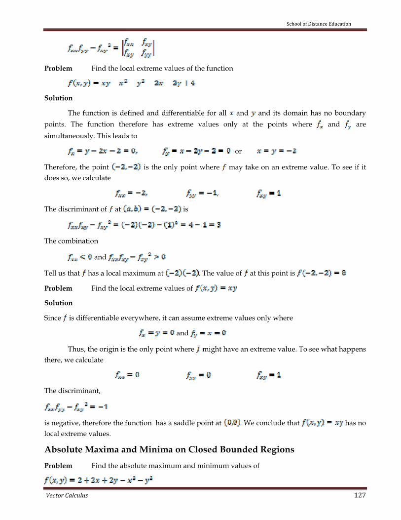
School of Distance Education
Vector Calculus 127
Problem Find the local extreme values of the function
Solution
The function is defined and differentiable for all and and its domain has no boundary points. The function therefore has extreme values only at the points where and are simultaneously. This leads to
or
Therefore, the point is the only point where may take on an extreme value. To see if it does so, we calculate
,
The discriminant of at is
The combination
and
Tell us that has a local maximum at . The value of at this point is
Problem Find the local extreme values of
Solution
Since is differentiable everywhere, it can assume extreme values only where
and
Thus, the origin is the only point where might have an extreme value. To see what happens there, we calculate
The discriminant,
is negative, therefore the function has a saddle point at . We conclude that has no local extreme values.
Absolute Maxima and Minima on Closed Bounded Regions Problem Find the absolute maximum and minimum values of

School of Distance Education
Vector Calculus 128
on the triangular plate in the quadrant bounded by the lines
Solution
Since is differentiable, the only places where can assume values are points inside the triangle where and point the boundary.
Interior Points For these we have
Yielding the single point The value of there is
Boundary Points We take the triangle one side at a time.
1. On the segment The function
may now be regarded as a function of defined on the closed interval Its extreme values may occur at the endpoints.
where
where
and at the interior points where is where
2.On the segment OB, and
We know from the symmetry of in and and from the analysis we just carried out that the candidates on this segment are
We have already accounted for the values of at the endpoints of so we need only look at the interior points of With , we have
Setting gives
At this value of
and
We list all the candidates: . The maximum is 4, which assumes at The minimum is which assumes at and .

School of Distance Education
Vector Calculus 129
Assignments
Find all the local maxima, local minima and saddle points of the functions in Assignments 1-15
1.
2.
3
4.
5
6
7.
8.
9
10
11.
12.
13
14
15
In Assignments 16-19, find the absolute maxima and minima of the functions on the given domain.
16 on the closed triangular plate bounded by the lines in the first quadrant.
17 on the closed triangular plate in the first quadrant bounded by the lines
18 on the rectangular plate
19 on the rectangular plate
20 Find two numbers a and b with such that
has its largest value.
22 Find the maxima, minima and saddle points of if any, given that
a) and
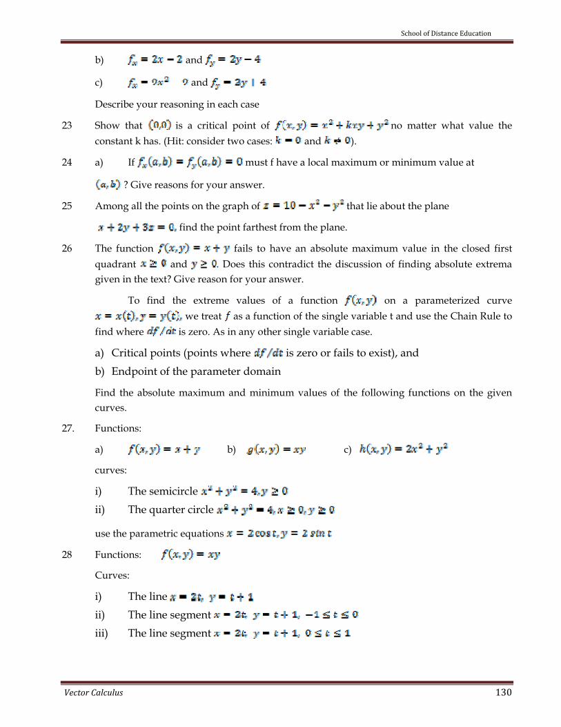
School of Distance Education
Vector Calculus 130
b) and
c) and
Describe your reasoning in each case
23 Show that is a critical point of no matter what value the constant k has. (Hit: consider two cases: and ).
24 a) If must f have a local maximum or minimum value at
? Give reasons for your answer.
25 Among all the points on the graph of that lie about the plane
find the point farthest from the plane.
26 The function fails to have an absolute maximum value in the closed first quadrant and . Does this contradict the discussion of finding absolute extrema given in the text? Give reason for your answer.
To find the extreme values of a function on a parameterized curve we treat as a function of the single variable t and use the Chain Rule to
find where is zero. As in any other single variable case.
a) Critical points (points where is zero or fails to exist), and b) Endpoint of the parameter domain
Find the absolute maximum and minimum values of the following functions on the given curves.
27. Functions:
a) b) c)
curves:
i) The semicircle ii) The quarter circle
use the parametric equations
28 Functions:
Curves:
i) The line ii) The line segment iii) The line segment

School of Distance Education
Vector Calculus 131
LAGRANGE MULTIPLIERS In this chapter we consider the method of Lagrange multipliers to solve max-min problems with constrained variables.
Constrained Maxima and Minima
Problem Find the point closest to the origin on the plane
Solution
The problem asks us to find the minimum value of the function
Subject to the constraint that
Since has a minimum value wherever the function
has a minimum value, we solve the problem by finding the minimum value of subject to the constraint . If we regard and as the independent variables in this equation and write as
our problem reduces to one of finding the points at which the function
has its minimum value or values. Since the domain of is the entire - plane, the first derivative test of the previous chapter tells us that any minima that might have must occur at points where
This leads to
and the solution
We may apply a geometric argument together with the second derivative test to show that these values minimize . The z coordinate of the corresponding point on the plane is
Therefore, the closest point we seek is
The distance from to the origin is

School of Distance Education
Vector Calculus 132
Remark Attempts to solve a constrained maximum or minimum problem by substitution, as we might call the method of Problem 1, do not always go smoothly. Hence the need of the method of Lagrange multipliers. Before formally give the Lagrange method we consider as Problem.
Problem Find the points closest to the origin on the hyperbolic cylinder
Solution
To find the points on the hyperbolic cylinder closest to the origin we imagine a small sphere centered at the origin expanding like a soap bubble until it just touches the hyperbolic cylinder At each point of contact, the hyperbolic cylinder and sphere have the same tangent plane and normal line. Therefore, if the sphere and cylinder are represented as the level surfaces obtained by setting.
and equal to 0, then the gradient vectors and (being normal’s to the surfaces at the point of contact) will be parallel where the surfaces
touch. At any point of contact we should therefore be able to find a scalar such that
or
Thus, the coordinates and of any point of tangency will have to satisfy the three scalar equations.
……(1)
For what values of will a point whose coordinates satisfy the equations in (1) also lie on the surface ? To answer this equation, we use the fact that no point on the surface has a zero x- coordinates to conclude that in the first equation in (1). This means that
only if
or
For , the equation becomes . If this equation is to be satisfies as well as z must be zero. Since also (from the equation ), we conclude that the points we seek all have coordinates of the form
What points on the surface have coordinates of this form? The points for which
, ,
The points on the cylinder closest to the origin are the points .
The Method of Lagrange Multipliers
Theorem 1 (The Orthogonal Gradient Theorem)
Suppose that is differentiable in a region whose interior contains a smooth curve

School of Distance Education
Vector Calculus 133
If is a point on where has a local maximum or minimum relative to its values on then is orthogonal to at
Proof We show that is orthogonal to the curve’s velocity vector at The values of on are given by the composite , whose derivative with respect to is
At any point where has a local maximum or minimum relative to its values on the curve,
so
By dropping the z- terms in Theorem I, we obtain a similar result for functions of two variables.
Corollary of Theorem 1 At the points on a smooth curve where a differentiable function takes on its local maxima and minima relative to its values on the curve,
Theorem 1 is the key to the method of Lagrange multipliers. Suppose that and are differentiable and that is a point on the surface where has a local maximum or minimum value relative to its other vales on the surface. Then takes on a local maximum or minimum at relative to its values on every differentiable curve through on the surface
. Therefore, is orthogonal to the velocity vector of every such differentiable curve through But so is (because is orthogonal to the level surface as seen in the chapter ‘Directional Derivatives’). Therefore, at . is some scalar multiple is called Lagrange Multiplier.
The Method of Lagrange Multipliers
Suppose that and are differentiable. To find the local maximum and minimum values of subject to the constraint find the values of and that simultaneously satisfy the equations
and
For functions of two independent variables, the appropriate equations are
and
Problem Find the greatest and smallest values that the function
takes on the ellipse
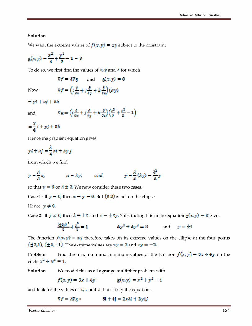
School of Distance Education
Vector Calculus 134
Solution
We want the extreme values of subject to the constraint
To do so, we first find the values of and for which
and
Now
and
Hence the gradient equation gives
from which we find
so that or . We now consider these two cases.
Case 1 : If , then But is not on the ellipse.
Hence, .
Case 2: If , then and Substituting this in the equation gives
and
The function therefore takes on its extreme values on the ellipse at the four points , . The extreme values are and
Problem Find the maximum and minimum values of the function on the circle
Solution We model this as a Lagrange multiplier problem with
,
and look for the values of and that satisfy the equations

School of Distance Education
Vector Calculus 135
The gradient equation implies that and gives
These equations tell us, among other things, that and have the same sign. With these values for and the equations
gives
so and
Thus, ,
and has extreme values at
By calculating the value of at the points , we see that its maximum and minimum
values on the circle are
and
Lagrange Multipliers with Two Constraints
Many problems require us to find the extreme value of a differentiable function whose variables are subject to two constraints. If the constraints are
and
and and are differentiable, with not parallel to , we find the constrained local maxima and minima of by introducing two Lagrange multipliers and . That is, we locate the points where takes on its constrained extreme values by finding the values of and that simultaneously satisfy the equations
….(2)
Problem The plane cuts the cylinder in an ellipse Find the point on the ellipse that lie closest to and farthest from the origin.
Solution
We find the extreme values of
[The square of the distance from (x,y,z) to the origin] subject to the constraints
…(3)

School of Distance Education
Vector Calculus 136
……(4)
The gradient equation in (2) then gives
or ….(5)
The scalar equations in (5) yield
…..(6)
Equations (6) are satisfied simultaneously if either and or and
If , then solving Eqs. (6) are satisfied simultaneously if either and or .
If then solving Eqs (3) and (4) simultaneously to find the corresponding points on the ellipse gives the two points and .
If he Eqs (3) and (4) give
The corresponding points on the ellipse are
and
But here we need to be careful. While and both give local maxima of on the ellipse, is farther from the origin than . The points on the ellipse closest to the origin are and . The point on the ellipse farthest from the origin is . Assignments 1. Find the points on the ellipse where has its extreme values 2. Find the maximum value of on the line 3 Find the points on the curve nearest the origin. 4 Use the method of Lagrange multipliers to find a) the minimum value of subject to the constraints ;
b) the maximum value of subject to the constraint

School of Distance Education
Vector Calculus 137
5 Find the dimensions of the closed right circular cylindrical can of smallest surface area whose volume is .
6 Use the method of Lagrange multipliers to find the dimensions of the rectangle of greatest area that can be inscribed in the ellipse with sides parallel to the coordinate axes.
7 Find the maximum and minimum values of subject to the constraint .
8 The temperature at a point on a metal plate is . An ant on the plate walks around the circle of radius 5 centered at the origin. What are the highest and lowest temperatures encountered by the ant?
9 Find the point on the plane closest to the point . 10 Find the minimum distance from the surface to the origin. 11 Find the point on the surface closest to the origin. 12 Find the maximum and minimum values of on the sphere
. 13 Find three real numbers whose sum is 9 and the sum of whose squares is as small as possible. 14 Find the dimensions of the closed rectangular box with maximum volume that can be
included in the unit sphere. 15 A space probe in the shape of the ellipsoid enters the earth’s
atmosphere and its surface begins to heat. After one hour, the temperature at the point on the probe’s surface is Find the hottest point
on the probe’s surface. 16 (Application to economics) In economics, the usefulness or utility of amounts and of two
capital goods and is sometimes measured by a function . For Problem, and might to be two chemicals a pharmaceutical company needs to have on hand and
the gain from manufacturing a product whose synthesis requires different amounts of the chemicals depending on the process used. If costs dollars per kilogram, costs dollars per kilogram, and the total amount allocated for the purchase of and together is dollars, then the company’s managers want to maximize given that . Thus, they need to solve a typical Lagrange multiplier problem. Suppose that and that the equation simplifies to
. Find the maximum value of and the corresponding values of and subject to this latter constraint.
17 Maximize the function subject to the constraints and
18 Find the point closets to the origin on the line of intersection of the planes and
19 Find the extreme values of on the intersection of the plane with the sphere
20 Find the extreme values of the function on the circle in which the plane intersects the sphere

School of Distance Education
Vector Calculus 138
MODULE ‐III MULTIPLE INTEGRALS
DOUBLE INTEGRALS: INTEGRTION OF FUNCTIONS OF TWO INDEPENDENT VARIABLES
Integration of functions of two Variables – Double integration
Let be a continuous function of two variables and
defined on a region bounded by a closed curve
Let the be divided, in any manner, into sub-regions of areas . Let be any point in the sub region of area and consider the sum
Limit of theabove sum is defined as the double ntegral of over the region R, written mathematically as follows :
….(1)
The region is called the region of integration (this region corresponds to the interval of
integration in the case of definite integral of the form of a function of single
variable). In order to simplify the evaluation of the double integral we often consider sub regions of and one common choice is the rectangular sub regions or rectangular grids, obtained by subdividing by lines parallel to the coordinate axes. Since the area of a typical rectangular grid is
, it follows from (1) that
Properties of Double Integrals
(1) for any number k
(2) y)dA
(3) if f(x,y) on R
(4) if on
(5) =
Where and
Property 3 above is called domain in additivity property.
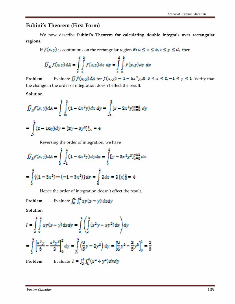
School of Distance Education
Vector Calculus 139
Fubini’s Theorem (First Form) We now describe Fubini’s Theorem for calculating double integrals over rectangular
regions.
If is continuous on the rectangular region then
Problem Evaluate for . Verify that the change in the order of integration doesn’t effect the result.
Solution
Reversing the order of integration, we have
Hence the order of integration doesn’t effect the result.
Problem Evaluate
Solution
Problem Evaluate

School of Distance Education
Vector Calculus 140
Solution
Fubini’s Theorem (Stronger form) We now describe Fubini’s Theorem for calculating double integrals over bounded non-
rectangular regions.
Let is continuous on a (rectangular or non-rectangular) region R.
1. If R is defined by
with and continuous on then
2. If R is defined by
with and continuous on then
Remark In I above integration is first with respect to while in 2 integration is first with respect to .
Problem Evaluate
Problem Calculate where is the triangle in the plane bounded by the axis, the
line and the line whether changing the order of integration works.

School of Distance Education
Vector Calculus 141
Solution
The region of integration is determined in Problem 2. The region is given by the following system of inequalities:
If we integrate first with respect to and then with respect to , we find
By Problem 2, The above system of inequalities representing the triangle is equivalent to the following:
If we consider this, then
and we are stopped by the fact that cannot be expressed in terms of elementary functions.
Hence in this Problem changing the order of integration doesn’t work.
Problem Evaluate over the first quadrant of the circle .
Solution
Here the circle meets the when and this implies Hence in the first quadrant the circle meets the line Consider strips parallel to the axis. Each strip varies
from to the curve To cover the entire region each strip move from to Hence the region enclosed in the first quadrant of the circle is given by the set of inequalities:
Problem Evaluate over the region in which and
Solution Region of integration is
(Ref. Problem 5)

School of Distance Education
Vector Calculus 142
Problem Evaluate where is the domain in the first quadrant of the circle
Solution Proceeding as in Problem 14, the region of integration is
Hence the required integral I is given by
……(1)
(Put in (1), then or when when
ProblemEvaluate by changing the order of integration.
Solution Here the region of integration of the double integral is given by
means of the following system of inequalities:
and ….(1)
Alternatively, the region of integration is (Ref. Problem 6)

School of Distance Education
Vector Calculus 143
and ….(2)
To change the order of integration (i.e., to evaluate the integral by integration first with respect to x) we have to consider the alternative form (2)
Problem Evaluate
Solution
=
Problem Evaluate
Solution

School of Distance Education
Vector Calculus 144
Assignments
1. 3.
2. 4.
5 6 .
7 8
9
10 Evaluate over the quadrant of the
11 Evaluate xydxdy where is the region of the circle
12 Evaluate where is
(i) the region in the first quadrant of the circle
(ii) the region in the first quadrant of the circle
14. Evaluate over the region in which each of and
15 Evaluate over the region in which each of and
16 Evaluate where is the triangle with vertices
17 Evaluate over the quadrant bonded by .
(Exercise 22 is a special case, with of this exercise)
18 Evaluate where is the region bounded by the axis, or
dinate and the parabola
19. Find the value of the integral taken over the postive quadrant of the ellipse
20 Evaluate where is the region bounded by the ellipse
21 Evaluate by changing the order of integration.
22 Change the order of integration in and hence evaluate the given
integral.
23. Change the order of integration in and hence evaluate the given integral.
24 Change the order of integration in and hence evaluate the given integral.

School of Distance Education
Vector Calculus 145
25 Change the order of integration in and hence evaluate the given integral.
26 Change the order of integration in and hence evaluate the given
integral.
27 Evaluate by changing the order of integration.
28. Evaluate by changing the order of integration.
29. Evaluate by changing the order of integration.
30. Evaluate by changing the order of integration.
31. Evaluate
32. Evaluate over the positive quadrant of the circle
and supposing .
33. Evaluate over the region in the positive quadrant for which
34. Show that
35. Show that
36. Show that
Hint:
37. Evaluate over the area bounded by the ellipse
38 Evaluate .
Applications of Double Integral Area by double Integral
Suppose it is required to find the area A enclosed between and
Let the area be divided into rectangle elements of the type of area , where and . If this elements is moved along the vertical strip from to
we obtain the area of that strip as

School of Distance Education
Vector Calculus 146
which represents the area of the vertical strip. Adding up all such strips between and , we get the required are as
Problem Find the area enclosed between and and .
Solution
Here and . So using the same idea just given above, we have
Problem Find the area bounded between the curve above the axisand below the line
Problem Find thearea enclosed by the ellipse
Solution Required area is where is the region enclosed by the ellipse .
i.e., the region of intregration is
Required area is given by
Assignments
1. Find the area enclosed by the lines
2 Find the area enclosed by the parabola and the axis.

School of Distance Education
Vector Calculus 147
3 Find the area in the first quadrant bounded by the axis and thecurves and
4 Find the area of the cardioid
5 Find by double integration, the area which lies inside the cardiod and outside the circle .
6 Find the area of the ellipse , using double integration.
7 Using double integration, find the area of the region enclosed by the parabola and the line
Volume by Double integral Volume of Solid of Revolution
We consider the area boudned by the lines and the x- axis Let this area revolve about the x-axis. To find this volume of the solid of revolution, which is generated, we consider, an elementary area , where . The area of the rectangle is
when revolve about the axis, the elementary area generates a hollow circular disk whose internal radius is and external radius is and thickness is so that its volume is
i.e., , as we can neglect the term
. Hencethe total volume is given by
Problem Find the volume of a spherical segment of height of a sphere of radius Deduce the volume of the solid enclosed by the sphere of radius
Solution The equation of the generating circle is , the centre being the origin and the x- axis being into plane, which cuts of the segment. The required solid is generated by rotating the region about the x-axis
Volume of the segmet is given by
The volume of the solid enclosed by the sphere is

School of Distance Education
Vector Calculus 148
obtained by taking so that its volume is
Assignments
1. Find the colume of the ellipsoid
2. Find the volume of the paraboloid of revolution cut off by the plane
3 Find the volume of the solid enclosed by the sphere
Volume of Solid as Double Integral Suppose is defind over a rectangular or non-rectangular region . Then we can interpert the double integral of over as the volume of the solid prism bounded below by and above by the surface Each term in the sum
is the volume of a vertical rectangular prism that approximates the volume of the portion of the solid that stands directly above the base . The limit of the sum is defined as the volume of the solid. That is
Volume =
Problem Find the volume enclosed by the co-ordinate planes and the portion of the plane in the first octant (Fig. 28)
Solution
In the first quadrant the values of are always greater than or equal to 0. The required volume is given by
zdxdy
Where and is region bounded by and i.e.,

School of Distance Education
Vector Calculus 149
DOUBLE INTEGRALS IN POLAR FORM
Integrals are sometimes easier to evaluate if we change to polar coordinates. The chapter shows how to accomplish this.
Problem Find the limits of integration for integrating over the region that lies inside the cardioids and outside the circle Also find the integral value when
Solution:
Step 1: (A sketch) We sketch the region and label the bounding curves (Fig.1)
Step 2: (The limits of integration) .A typical ray from the origin enters the region where
.
Step 3: (The limits of integration). The rays from the origin that intersect the region run from to
The integral is
If is the constant function whose value is I, then the integral of over is the area of
The area of a closed and bounded region in the polar coordinate plane is
….(1)
Changing Cartesian Integrals into Polar Integrals
The procedure for changing a Cartesian integral into a polar integral has two steps.
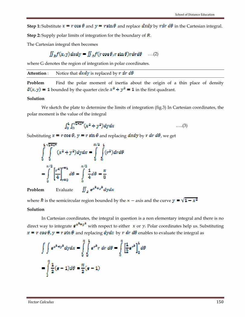
School of Distance Education
Vector Calculus 150
Step 1: Substitute and and replace by in the Cartesian integral.
Step 2: Supply polar limits of integration for the boundary of
The Cartesian integral then becomes
….(2)
where G denotes the region of integration in polar coordinates.
Attention : Notice that is replaced by
Problem Find the polar moment of inertia about the origin of a thin place of density bounded by the quarter circle in the first quadrant.
Solution
We sketch the plate to determine the limits of integration (fig.3) In Cartesian coordinates, the polar moment is the value of the integral
…..(3)
Substituting and replacing by , we get
Problem Evaluate
where is the semicircular region bounded by the axis and the curve
Solution
In Cartesian coordinates, the integral in question is a non elementary integral and there is no
direct way to integrate with respect to either or Polar coordinates help us. Substituting and replacing by enables to evaluate the integral as

School of Distance Education
Vector Calculus 151
Assignments
In Assignments 1-16, change the Cartesian integral into an equivalent polar integral. Then evaluate the polar integral.
1. 2.
3 4.
5 6.
7 8
9 10.
11 12
13 14
15 16
17 Find the area of the region cut from the first quadrant by the curve
.
18 Find the area enclosed by one leaf of the rose .
19 Find the area of the region cut from the first quadrant by the cardioids .
20 Find the area of the region that lies inside the cardioids and outside the circle
21 Find the area of the region enclosed by the positive x- axis and spiral . The region common to the interiors of the cardioids
and
TRIPLE INTEGRALS IN
RECTANGULAR COORDINATES
The Triple Integral of a function of three independent variables, over a surface is defined in the same manner as a double integral.

School of Distance Education
Vector Calculus 152
Properties of Triple Integrals
Triple integrals have the same algebraic properties as double and the single integrals. If and are continuous, then
1. = (any number k )
2. =
3. 0 if on
4 if on
Triple integrals also have an additivity property. If the domain of a continuous function is partiotioned by smooth surfaces into a finite number of non-overlapping cells then
= + +…….+
Application of Triple Integrals:
Volume by Triple Integrals
Definition The volume of a closed bounded region in space is
…..(1)
We also note that
Where is the region given by the system of inequalities:
Problem Evaluate
Solution
Problem Find the volume of the region enclosed by the surfaces
Solution

School of Distance Education
Vector Calculus 153
Using (1), the volume is
To find the limits of integration for evaluating the integral, we take the following steps.
Step 1 : (A sketch) The surfaces (fig. 1) intersect on the elliptical cylinder or . The boundary of the region , the projection of onto
the xy plane, is an ellipse with the same equation: The “upper” boundary of is the
curve . The lower boundary is the curve .
Step 2: (The z- limits of integration). The line passing through a typical point parallel to the z-axis enters at and leaves at
Step 3: (The y- limits of integration). The line through parallel to the y-axis enters
at and leaves at .
Step 4: (The x- limits of integration). As sweeps across (putting in we obtain and ) the value of varies from at to at
The volume of is

School of Distance Education
Vector Calculus 154
(now put )
.
Problem Evaluate where is the volume bounded by the planes
and
Solution (Fig.2) Here the region of integration is bounded by the planes to and i.e.,
Problem Using the idea of triple integral, find the volume of the solid enclosed by the sphere .
Solution
Because of symmetry, we need to complete the volume in the first octant only. Hence if is the total volume, then

School of Distance Education
Vector Calculus 155
Where is the region of the sphere in the first octant
Now the region of integration is such that
varies from to
varies from to varies from to
Assignments
Evaluate the integrals in Exercise 1-14
1.
2.
3.
4.
5.
6.
7.
8.

School of Distance Education
Vector Calculus 156
9.
10.
11.
12.
13.
14.
TRIPLE INTEGRALS IN CYLINDRICAL AND SPHERICAL COORDINATES
When a calculation in physics, engineering, or geometry involves a cylinder, cone or sphere, we can often simplify our work by using cylindrical or spherical coordinates.
Triple Integrals in Cylindrical Coordinates
In Cylindrical coordinates (Fig.1) the surfaces like the following have equations of constant coordinate values:
Cylinder, radius 4, axis the z-axis
Plane containing the z-axis

School of Distance Education
Vector Calculus 157
Plane perpendicular to the z-axis
The volume element (Fig.2) for subdividing a region in space with cylindrical coordinates is
Triple integrals in cylindrical coordinates are then evaluated as integrated integrals, as in the following Problem.
Problem 1 Find the limits of integration in cylindrical coordinates for integrating a function over the region D bounded below by the plane laterally by the circular cylinder
, and above by the paraboloid .
Solution
Step 1 : (A sketch) (Fig.3). The base of is also the region’s projection on the plane. The boundary of is the circle . It polar coordinate equation is obtained as follows:
r =2sin
Step 2: (The z- limits of integration). A line through a typical point in parallel to the z-axis enters at and leaves at (Here we have used the fact, with
and ,
Step 3: (The limits of integration). A ray through from the origin enters at and leaves at .

School of Distance Education
Vector Calculus 158
Step 4: (The limits of integration). As sweeps across , the angle it makes with the positive axis runs from to .
The integral is
…(2)
Problem 2 Find the centroid of the solid (with density given by ) enclosed by the cylinder bounded above by the paraboloid and below by the xy-plane.
Solution First we note that with and ,
We sketch the solid, bounded above by the paraboloid and below by the plane (Fig. 4). Its base is the disk in the xy-plane. (Details: corresponds to the xy-plane.
corresponds to and hence the base such that , that is ). The solid’s centeroid lies on its axis of symmetry, here the z-axis. This makes
To find we divide the first moment by the mass .
To find the limits of integration for the mass and moment integrals, we continue with the four basic steps. We completed step 1 with our initial sketch. The remaining steps give the limits of integration.
Step 2: (The z- limits). A line through a typical point in the base parallel to the z- axis enters the solids at and leaves
Step 3 : ( The r-limits ). A ray through from the origin enters at and leaves at
Step 4 : (The - limits). As sweeps over the base like a clock hand, the angle it makes with the positive x- axis runs from to . The value of is
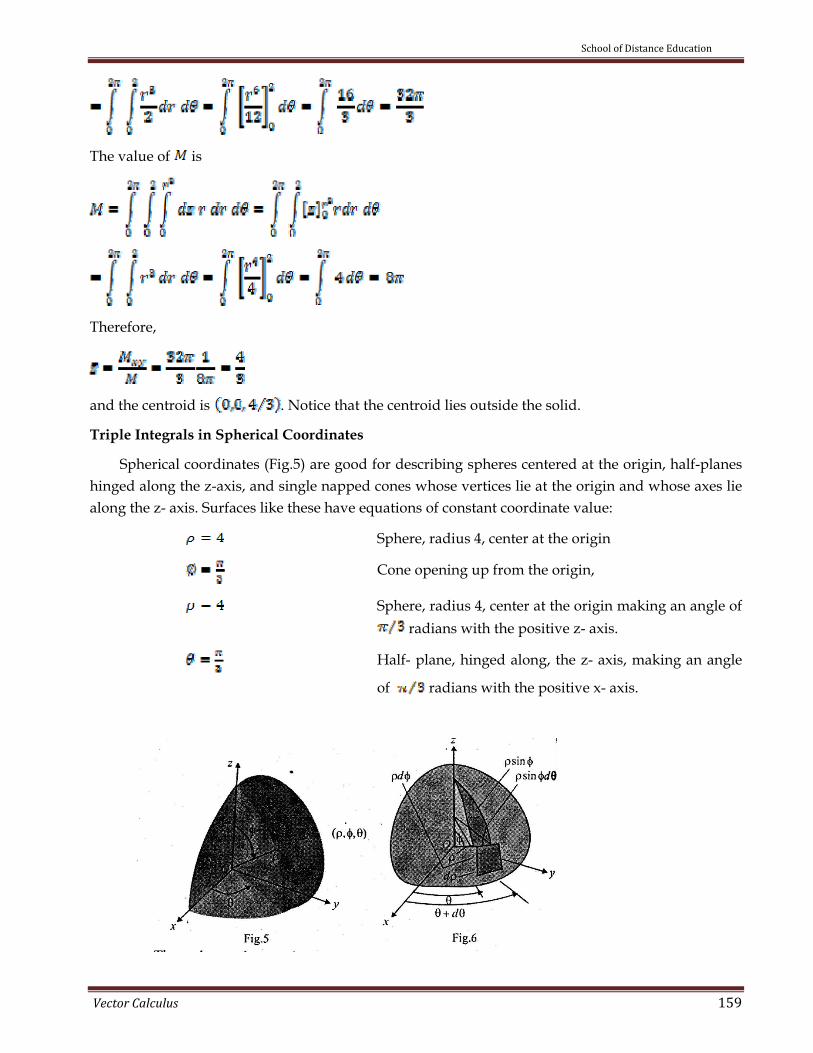
School of Distance Education
Vector Calculus 159
The value of is
Therefore,
and the centroid is . Notice that the centroid lies outside the solid.
Triple Integrals in Spherical Coordinates
Spherical coordinates (Fig.5) are good for describing spheres centered at the origin, half-planes hinged along the z-axis, and single napped cones whose vertices lie at the origin and whose axes lie along the z- axis. Surfaces like these have equations of constant coordinate value:
Sphere, radius 4, center at the origin
Cone opening up from the origin,
Sphere, radius 4, center at the origin making an angle of radians with the positive z- axis.
Half- plane, hinged along, the z- axis, making an angle
of radians with the positive x- axis.

School of Distance Education
Vector Calculus 160
The volume element in spherical coordinates is the volume of a spherical wedge defined by the differentials and (Fig.6) The wedge is approximately a rectangular box with one side a circular arc of length , another side a circular arc of length , and thickness . Therefore the volume element in sphere in spherical coordinates is
….(3)
and triple integrals take the form
…(4)
In particular, the volume of a region in space is given by (with
V= …(5)
To evaluate these integrals, we usually integrate first with respect to . The procedure for finding the limits of integration is illustrated in the following Problem. We restrict our attention to integrating over domains that are solids of revolution about the z- axis (or portions thereof) and for which the limits for and are constant.
Problem 3 Find the volume of the upper region cut from the solid sphere by the cone
Solution
The volume is
To find the limits of integration for evaluating the integral, we take the following steps.
Step 1: (A sketch) We sketch and its projection on the plane (Fig.7)
Step 2 : (The limits of integration) We draw a ray from the origin making an angle with the positive z- axis. We also draw , the projection of on the xy-plane, along with the angle
that makes with the positive x- axis. Ray enters at and leaves at

School of Distance Education
Vector Calculus 161
Step 3: (The limits of integration). The cone makes an angle of with the positive z- axis. For any given , the angle can run from to .
Step 4: (The - limits of integration).The ray sweeps over as runs from to . The volume is
Problem 4 A solid of constant density occupies the region in Problem 3. Find the solid’s moment of inertia about the z- axis.
Solution In rectangular coordinates, the moment is
dv
In spherical coordinates, , Hence,
For the region in Problem 3, this become
Assignments
Evaluate the cylinder coordinated integrals in Assignments 1-5.
1. 2

School of Distance Education
Vector Calculus 162
3. . 4
5
6. Let be the region bounded below by the plane , above by the sphere and on the sides by the cylinder . Set up the triple integrals in cylindrical coordinates that give the volume of using the following orders of integration.
(a) (b) (c)
7 Give the limits of integration for evaluating the integral
as an iterated integral over the region that is bounded below by the plane on the side by the cylinder , and on top by the paraboloid
Evaluate the spherical coordinate integrals in Assignments 8-12.
8
9
10 .
11
12
13. Let be the region bounded below by the plane above by the sphere and on the sides by the cylinder give the volume of using the following orders of integration. a)d b)d
SUBSTITUTIONS IN MULTIPLE INTEGRALS In this chapter we show how to evaluate multiple integrals by substitution.
Substitutions in Double Integrals
Suppose that a region in the plane is transformed one-to-one into the region in the xy- plane by equations of the form
.
We call the image of under the transformation, and the pre image of Any function defined on can be thought of as a function defined on as well. Then
….(1)

School of Distance Education
Vector Calculus 163
The factor is the Jacobian determinant or Jacobian of the coordinate transformation defined by
….(2)
Notation The Jacobian is also denoted by
to help remember how the determinant in Eq(2) is constructed from the partial derivatives of and
Problem Evaluate
by applying the transformation
…(3)
and integrating over an appropriate region in the plane
Solution
(3) gives , . …..(4)
=
equations for the Corresponding equations Simplified ‐
Boundary of for the boundary of G equations
+1

School of Distance Education
Vector Calculus 164
Problem Evaluate
Solution
The integrand suggests the transformation and . That is,
….(5)
Substitutions in Triple Integrals Suppose that region in space is transformed one-to-one into the region in
space by differentiable equations of the form
as in Fig.4 on the next page Then any function defined on can be thought of as a function
equations for the Corresponding equations Simplified ‐
boundary of for the boundary of G equations
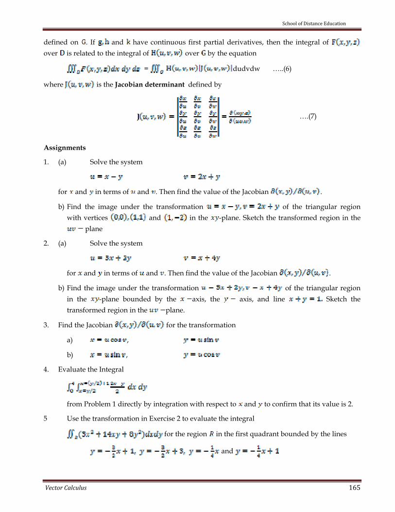
School of Distance Education
Vector Calculus 165
defined on . If and have continuous first partial derivatives, then the integral of over is related to the integral of over by the equation
= dudvdw …..(6)
where is the Jacobian determinant defined by
….(7)
Assignments
1. (a) Solve the system
for and in terms of and . Then find the value of the Jacobian .
b) Find the image under the transformation of the triangular region with vertices and in the -plane. Sketch the transformed region in the
plane
2. (a) Solve the system
for and in terms of and . Then find the value of the Jacobian .
b) Find the image under the transformation of the triangular region in the -plane bounded by the axis, the axis, and line Sketch the transformed region in the plane.
3. Find the Jacobian for the transformation
a) ,
b) ,
4. Evaluate the Integral
from Problem 1 directly by integration with respect to and to confirm that its value is 2.
5 Use the transformation in Exercise 2 to evaluate the integral
for the region in the first quadrant bounded by the lines
and

School of Distance Education
Vector Calculus 166
6 Let be the region in the first quadrant of the plane bounded by the hyperbolas and the lines Use the transformation with
and to rewrite
as an integral over an appropriate region in the plane. Then evaluate the integral over
7 A thin plate of constant density covers the region bounded by the ellipse in the plane. Find the first moment of the plate about
the origin. (Hint: use the transformation ).
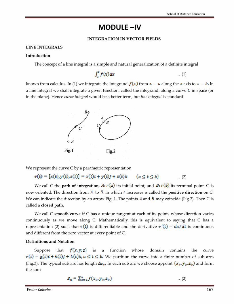
School of Distance Education
Vector Calculus 167
MODULE –IV INTEGRATION IN VECTOR FIELDS
LINE INTEGRALS
Introduction
The concept of a line integral is a simple and natural generalization of a definite integral
…(1)
known from calculus. In (1) we integrate the integrand from along the axis to In a line integral we shall integrate a given function, called the integrand, along a curve in space (or in the plane). Hence curve integral would be a better term, but line integral is standard.
We represent the curve C by a parametric representation
…(2)
We call C the path of integration, its initial point, and its terminal point. C is now oriented. The direction from to in which increases is called the positive direction on C. We can indicate the direction by an arrow Fig. 1. The points and may coincide (Fig.2). Then C is called a closed path.
We call C smooth curve if C has a unique tangent at each of its points whose direction varies continuously as we move along C. Mathematically this is equivalent to saying that C has a representation (2) such that is differentiable and the derivative is continuous and different from the zero vector at every point of C.
Definitions and Notation
Suppose that is a function whose domain contains the curve We partition the curve into a finite number of sub arcs
(Fig.3). The typical sub arc has length . In each sub arc we choose appoint and form the sum
…(2)

School of Distance Education
Vector Calculus 168
If is continuous and the functions and have continuous first derivatives, then the sums in (2) approach a limit as increases, and lengths approach zero. We call this limit the integral of over the curve from to . If the curve is denoted by a single letter, C for Problem, the notation for the integral is
….(3)
and read “the integral of over C”
Evaluation for Smooth Curves
If is smooth for (i.e., if is continuous and never 0), we can use the equation (obtained from Eq. (5) of chapter “Arc Length and the Unit Tangent Vector T” with
to express in Eq(3) as . A theorem from advanced calculus says that we can then evaluate the integral of over C as
……(4)
This formula will evaluate the integral correctly no matter what parameterization we use, as long as the parameterization is smooth.
Problem Integrate over the line segment C joining the origin and the point . (Fig.4)
Solution
We choose the simplest parameterization we can think of :
The components have continuous first derivatives and is never 0, so the parameterization is smooth. The integral of over C is

School of Distance Education
Vector Calculus 169
Additivity
Line integrals have the useful property that if a curve is made by joining a finite number of curves end to end, then the integral of a function over is the sum of the integrals over the curves that make it up
= + +……..+ …..(6)
...(6)
Mass and Moment Calculations
Mass and Moment formulas for coil springs, thin rods and wires lying along a smooth curve in space are given below:
Mass :
First moments about the coordinate planes:
,
Coordinates of the center of mass:
, ,
Moments of Inertia:
distance from the point to line
Radius of gyration about a line
Problem A coil spring lies along the helix
The spring’s density is a constant, Find the spring’s mass and center of mass, and its moment of inertia and radius of gyration about the axis.
Solution
Because of the symmetries involved, the center of mass lies at the point on the z- axis.

School of Distance Education
Vector Calculus 170
For the remaining calculations, we first find
Then
Notice that the radius of gyration about the z- axis is the
radius of the cylinder around which the helix winds.
Problem A slender metal arch, denser at the bottom than top, lies along the semicircle in the yz-plane . Find the center of the arch’s mass if the density at the point
on the arch is
Solution
We know that and because the arch lies in the -plane with its mass distributed symmetrically about the z-axis. To find , we parameterize the circle as
For this parameterization
Then, we obtain
= = =2

School of Distance Education
Vector Calculus 171
With to the nearest hundredth, the center of mass is
Assignments
1 Evaluate where C is the straight line segment from to .
2 Evaluate along the curve
.
3 Find the line integral of over the straight line segment from to .
4 Integrate over the path from and given by
5 Integrate over the path
In the following assignemnts, integrate f over the given curve
6
7 in the first quadrant from to
8 Find the mass of a wire that lies along the curve , if the density is .
9 Find the mass of a thin wire lying along the curve
if the density is
10 A circular wire hoop of constant density lies along the circle in the xy-plane. Find the hoop’s moment of inertia and radius of gyration about the z- axis.
VECTOR FIELDS, WORK, CIRCULATION AND FLUX
Scalar Field
Definition (Scalar fields) A scalar field is a scalar valued function of three variables. i.e. if to each point of a region in space there corresponds a unique scalar . We say that is a scalar field.
If is a scalar field, any surface defined by , where c is a constant, is called an isotimic surface or a level surface. For Problem, in Physics, if denotes either or gravitational field

School of Distance Education
Vector Calculus 172
potential, such surfaces are called equipotential surfaces. If denotes temperature, they are called isothermal surfaces.
Vector fields Definition (Vector field) A vector field is a vector valued function of three variables. i.e. vector field F is a rule associating with each point of a region in space, unique vector . A field three –dimensional vectors might have a formula like
The field is continuous if the components functions and are continuous, differentiable if and are differentiable, and so on. A field of two-dimensional vectors might have a formula like
Definition The gradient field of differentiable scalar functions is the field gradient vectors
Problem Find the gradient field of
Solution
The gradient field of is the
Problem Find the unit normal to the surface at the point
Solution This is level surface for the function grad is normal to the given surface.
Now
at the point
Hence a unit normal to the surface is
Note: Another unit normal is having direction opposite to the unit normal vector in the
Problem
Problem If
…(1)

School of Distance Education
Vector Calculus 173
Find , such that
Solution We have ….(2)
From (1) and (2) ….(3)
…(4)
…(5)
Integrating (3) with respect for x, we get
….(6)
where is free from x, arbitrary constant.
Differentiating (6) partially with respect to y and using (4), we get
. Then
….(7)
Now integrating (7) with respect to y, we get . So (6) is
..(8)
Differentiating (8) partially with respect to z and using (5), we get
Hence or a constant.
Therefore (8) becomes,
Given Here or or
Hence
The Work Done by a Force over a Curve in Space Suppose that the vector field represents a force throughout a region in space (it might be the force of gravity or an electromagnetic force of some kind) and that
is a smooth curve in the region. Then the integral of , the scalar component of in the direction of the curve’s unit tangent vector,
over the curve is called the work done by over the curve from to .
Definition The work done by a force

School of Distance Education
Vector Calculus 174
over a smooth curve from to is
….(1)
Derivation of (I):
The work done by along the curve segment (Fig.2) will be approximately
The work done by along the curve to will be approximately
As the norm of the partition of approaches zero, the norm of the induced partition of the curve approaches zero and these sums approach the line integral
The sign of the number we calculated with this integral depends on the direction in which the curve traversed as increases. If we reverse the direction of motion, we reverse direction of T and change the sign of and its integral.
Problem Find the work done by over the curve from to (Fig.3)
Solution
Step 1: (Evaluate F on the curve)
.
Step 2: (Find )
Step 3: (Dot F with )
Step 4: (Integrate from to )
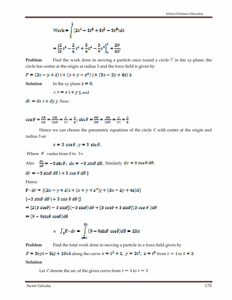
School of Distance Education
Vector Calculus 175
Problem Find the work done in moving a particle once round a circle in the xy-plane: the circle has centre at the origin at radius 3 and the force field is given by
Solution In the xy plane
, and
Now
Hence we can choose the parametric equations of the circle with center at the origin and radius 3 as:
Where varies from 0 to
Also Similarly
Hence
Problem Find the total work done in moving a particle in a force field given by
along the curve from to
Solution
Let denote the arc of the given curve from to

School of Distance Education
Vector Calculus 176
Work done is given by
Given
is in the parametric form ,y=2t2, z=t3
substituting etc. in the above we get
In the line integral varies from to
unit of work
Problem Find the value of (3) when and is the helix
... (4)
Solution
From (4) we have
Thus
Hence (3) gives
Problem If evaluate where is:
(i) is a curve from to with parametric form
(ii) is the straight line joining and
Solution

School of Distance Education
Vector Calculus 177
Here
...(5)
(i) C is in the parametric form . At the point and at . Substituting in (5) we get
Moving from the point to means from to and Therefore
(ii) The straight line joining to is given in the parametric form by and varies from to Substituting in (5) we
get
in varies from to .
Problem Evaluate the line integral (3) with
along two different paths with the same initial point and the same terminal point , namely
(a) the straight line segment and (b) the parabolic arc
By substituting into F we obtain
We also need Hence the integral over is

School of Distance Education
Vector Calculus 178
b) Similarly, by substituting into F and calculating we obtain for the integral over the path .
Flow Integrals and Circulation
Definition If is a smooth curve in the domain of a continuous velocity field the flow along the curve from
to is the integral of over the curve from to .
…(2)
The integral in this case is called a flow integral. If the curve is a closed loop, the flow is called the circulation around the curve.
Problem A fluid’s velocity field is Find the flow along the helix .
Solution
Step 1: (Evaluate F on the curve)
Step 2: (Find )
Step 3:
Step 4:

School of Distance Education
Vector Calculus 179
Problem 14 Find the circulation of the field around the circle
Solution
1. On the circle,
2.
3.
1
4. Circulation=
Flux Across a Plane Curve Definition If C is a smooth closed curve in the domain of a continuous vector field
in the plane, and if n is the outward-pointing unit normal vector C, the flux of F across C is given by the following line integral:
….(3)
The Formula for calculating Flux Across a Smooth Closed Plane Curve
…(4)
The integral can be evaluated from any smooth parameterization that traces C counter clockwise exactly once.
Problem Find the flux of across the circle in the plane.
Solution
The parameterization , traces the circle clockwise exactly once. We can therefore use this parameterization in Eq(4). With
We find

School of Distance Education
Vector Calculus 180
The flux of F across the circle is Since the answer is positive, the net flow across the curve is outward. A net inward flow would have given a negative flux.
Assignments
Find the gradient fields of the functions in Exercise 1-2
1.
2.
3. Give a formula for the vector field in the plane that has the property that F points towards the origin with magnitude inversely proportional to the square of the distance from to the origin.
In Assignments 4-7find the work done by force F from to over each of the following paths.
a) The straight line path b) The curved path c) The path consisting of the segment from to followed by the
segment from to
4. 5.
6
In Assignments 7-8 find the work done by F over the curve in the direction of increasing t.
7
8
9 Evaluate along the curve from to
10 Evaluate for the vector field along the curve from
to
11 Find the work done by the force over the straight line from to
12 Find the circulation and flux of the fields
and

School of Distance Education
Vector Calculus 181
around and across each of the following curves.
(a) The circle (b) The ellipse
In Assignments 13-14 find the circulation and flux of the field F around and across the closed semicircular path that consists of the line segment
, followed by the line segment
13 14
15 Evaluate the flow integral of the velocity field along each of the following paths from to in the xy- plane.
a) The upper half of the circle
b) The line segment from to
c) The line segment from to followed by the line segment from to
In Assignments 16-17, F is the velocity field of a fluid flowing through a region in space. Find the flow along the given curve in the direction of increasing t
16
17
18 Find the circulation of around the closed path consisting of the following three curves traversed in the direction of increasing t:
19. The field is the velocity field of a flow in space. Find the flow from to along the curve of intersection of the cylinder and the plane .
(Hint: Use as the parameter).
PATH INDEPENDENCE, POTENTIAL FUNCTIONS
AND CONVERSATIVE FIELDS
In gravitational and electric fields, the amount of work it takes to move a mass or a charge from one point two another depends only on the object’s initial and final positions and not on the path taken in between. This chapter discusses the notion of path independence of work integrals and describes the remarkable properties of fields in which work integrals are path independence,

School of Distance Education
Vector Calculus 182
Definitions Let F be a field defined on an open region D in space, and suppose that for any two
points A and B in the D the work done in moving from A to B is the same over all paths
from A to B. Then the integral is path independent in D and the field F is conservative on D.
Definition If F is a field defined on D and for some scalar function on D, then is called a potential function for F.
Theorem 1, (The Fundamental Theorem of Line Integrals)
1. Let be a vector field whose components are continuous throughout an open connected region D in space. Then there exists a differentiable function such that
If and only if all points A and B in D the value of is independent of the path
joining A to B in D. 2. If the integral is independent of the path from A to B, its value is
Prove that implies path independent of the integral.
Proof. Suppose that A and B are two points in D and that C: r(t)=
is a smooth curve in D joining A and B. Along the curve, is a differentiable function of and
using chain rule
, because
Therefore,
Thus, the value of the work integral depends only on the values of at A and B and not on the path in between.
Remark In between proving the result, we have proved Part 2 as well as the forward implication in Part 1. The more technical proof of the reverse implication is omitted.
Problem Find the work done by the conservative field

School of Distance Education
Vector Calculus 183
along any smooth curve C joining the point to
Solution
With we have
as
by Part 2 of Fundamental Theorem
Problem Evaluate the integral
from to by showing that F has a potential and applying (3)
Solution
Recall that the vector field F has a potential if
grad
i.e., (here) if
i.e, if
i.e., (here) if
We show that we can satisfy these conditions.
Integrating with respect to we obtain
Where is an arbitrary function of and (and not involving Now differentiating with respect to we obtain
But it is given that
Hence
Integrating with respect to y, we obtain
Where is a function involving alone.

School of Distance Education
Vector Calculus 184
Differentiating with respect to z
Hence Hence h is a constant; say
This gives
and by (3)
Theorem 2
The following statements are equivalent:
1. around every closed loop in D.
2. The field F is conservative on D
Proof.
We want to show that for any two points A and B in D the integral of F.dr has the same value over any two paths and from A to B. We reverse the direction on to make a path from B to A. (Fig.1) Together, and to make a closed loop C and
Thus the integrals over and give the same value.
We want to show that the integral of is zero over any post loop C. We pick two points A and B on C and use them to break C in to two pieces from A and B followed by from B back to A. (Fig.2). Then

School of Distance Education
Vector Calculus 185
Finding Potentials for Conservative Fields
Now we give a test for being conservative.
The Component Test for Conservative fields
Let be a field whose component functions have continuous first partial derivative. Then, Fis conservative if and only if
and …(1)
Proof. We show that Eqs. (1) must hold if F is conservative. There is a potential function such that
as continuity implies that the mixed partial derivatives are equal
The other two equations in (1) are proved similarly.
The second half of the proof, that Eq.(1) imply that F is conservative, is a consequence of Stokes’s Theorem and is omitted.
Problem Show that is conservative and find a potential function for it.
Solution
We apply the test in Eqs. (1) to
and calculate
Together, these equalities tell us that there is a function with
We find by integrating the equations
…..(2)
We integrate the first equation with respect to holding and fixed, to get

School of Distance Education
Vector Calculus 186
We write the constant of integration as a function of and because its value may change if and change. We then calculate from this equation and match it with the expression for z
in Eq.(2). This gives
So Therefore, g is a function of z alone and
We now calculate from this equation and match it to the formula for in Eq.(2). This gives
or
Integration yields,
Hence
We have found infinitely many potential functions for F, one for each value of C.
Problem Show that is not conservative.
Solution
We apply the component test in Eqs (1) and final that
The two are unequal, so F is not conservative. No further testing required.
Exact Differential Forms
Definitions
The form is called a differential form. A differential form is exact on a domain D in space if
For some (scalar) function throughout D
Notice that if on D, then is gradient field of on . Conversely, if then the form is exact. The test for the form’s being exact is therefore the same as the test for being conservative.
Problem Show that the differential form under the integral sign of
I=

School of Distance Education
Vector Calculus 187
is exact, so that we have independence of path in any domain, and find the value of I from to
Solution
Here
Exactness follows from , which gives
To find we integrate (which is “long”, so that we save work) and then differentiate to compare with and
Integrating with respect to where is a function of z alone (Already , hence is not involved in the function ).
and hence so that, is a constant. Taking we have
From this and (5) we get
Problem Show that is exact, and evaluate the integral
over the line segment from to
Solution
We let and apply the test of Eq.(3):
These equalities tell us that is exact, so

School of Distance Education
Vector Calculus 188
for some function and the integral’s value is .
We find up to a constant by integrating the equations
…(4)
From the first equation we get
The second equation tells us that
or
Hence, g is a function of z alone, and
The third of Eqs. (4) tells us that
or .
Therefore,
The value of the integral is
Assignments
Which fields in Assignments 1-3 are conservative, and which are not ?
1. 2
3
In Exercise 4-6 find a potential function for the field F.
4. 5
6
In Exercise 7-11, show that the differential forms in the integrals are exact. Then evaluate the integrals.
7
8
9
10 11

School of Distance Education
Vector Calculus 189
12 Evaluate the integral from Problem 4 by finding parametric for the
line segment from to and evaluating the line integral of along the segment. Since F is conservative, the integral is independent of the path.
GREEN’S THEOREM IN THE PLANE
We need to ideas for Green’s theorem. The first is the flux density of a vector field at a point which in mathematics is called the divergence of the vector field. The second one is the idea of circulation density of a vector field, which in mathematics is called the curl of the vector field.
Definition The flux density or divergence of a vector field at the point is
...(1)
Problem Find the divergence of
Solution We use the formula in Eq.(1) :
Definition The circulation density or curl of a vector field at the point is
……(2)
Problem Find the curl of the vector field
Solution We use the formula (2) :
Green’s Theorem in the Plane
Theorem 1: Green’s Theorem (Flux-Divergence or Normal Form) The outward flux of a field across a simple closed curve equals the double integral of div F over the region
enclosed by That is,
…(3)
Theorem 2: Green’s Theorem (Circulation-Curl Tangential Form) The counter clockwise circulation of a field around a simple closed curve in the plane equals the double integral of curl over the region enclosed by That is,
….(4)
Problem Verify both forms of Green’s theorem for the field

School of Distance Education
Vector Calculus 190
and the region bounded by the unit circle
Solution
We first express all functions, derivatives, and differentials in terms of
L.H.S of Eq.(3) :
R.H.S of Eq.(3) :
Hence Theorem 1 is verified.
L.H.S of Eq.(4) :
R.H.S of Eq.(4) :
Hence Theorem 2 is verified
Using Green’s Therom to evaluate line integrals Problem Evaluate the line integral
Where C is the square cut from the first quadrant by the lines x=1 and y=1

School of Distance Education
Vector Calculus 191
Solution
We can use either from of greens theorem to change the line integral in to a double integral over the square.
1. With eq. (3) : Taking and and as the square’s boundary and interior gives (nothing that the region is given by the system of inequalities
2. With Eq.(4): Taking and gives the same result:
Extending Green’s Theorem to other Regions
Green’s theorem can be extended to regions of the form annular disk etc. The method is illustrated through Problems.
Problem Verify the circulation form of Green’s theorem on the annular ring (Fig. 2), if
Solution
The boundary of consists of the circle
traversed counter clockwise as increases, and the circle

School of Distance Education
Vector Calculus 192
Traversed clockwise as increases. The functions and and their parial derivatives are continuous throughout , Moreover,
The integral of over the boundary of is
d
Calculating Area with Green’s Theorem
If a simple closed curve in the plane and the region it encloses satisfy the hypotheses of Green’s theorem, the area of is given by the following Green’s Theorem Area formula.
Green’s Theorem Area Formula
Area of ….(5)
The reason is that by Eq.(3) run backward,
Area of
Area of a plane region as a line integral over the boundary
In the equation (1) of Green’s theorem choose and obtain
Also, setting we get
Now the double integral is the area of of By addition, we have
…(4)
where we integrate as indicated in Green’s theorem. This interesting formula expresses the area of in terms of a line integral over the boundary. It has various application; for instance, the theory of certain planimeters (instruments for measuring area) is based on it.

School of Distance Education
Vector Calculus 193
Problem For an ellipse or we get
thus from (4) we obtain the familiar result
Assignments
In Assignments 1-2 verify Green’s theorem by evaluating both sides of Eqs. (3) and (4) for the field Take the domains of integration in each case to be the disk and its
bounding circle
1. 2.
In Assignments 3-5, use Green’s theorem to find the counterclockwise circulation and outward flux for the field F and curve
3.
The square bounded by
4
The Triangle bounded by
5
The right hand loop of the lemniscates
6 Find the counter clockwise circulation and outward flux of the field around and over the boundary of the region enclosed by the curves and in the first quadrant.
7. Find the outward flux of the field
Across the cardioids
8. Find the work done by in moving a particle once counterclockwise around the curve.
The boundary of the “triangle” region in the first quadrant enclosed by the x-axis, the line , and the curve
Apply Green’s theorem to evaluate the integrals in Assignments 9-10
9.
The triangle bounded by

School of Distance Education
Vector Calculus 194
10
The circle
Use the Green’s theorem area formula (5) to find the area of the regions enclosed by the curves Assignments 11-12
11 The circle
12 The asteroid
SURFACE AREA AND SURFACE INTEGRALS
In this chapter our objective is the integration of function defined over a curved surface. For that purpose we first consider the surface area.
The Formula for Surface Area
The area of the surface over a closed and bounded plane region is
Surface area = …(1)
where p is a unit vector normal to and
That is, the surface area of the surface is the double integral over of the magnitude divided by the magnitude of the scalar component of normal to
Attention! Eq.(1) is obtained under the assumption that through out that is continuous. Whenever the integral exists, however, we define its value to be the area of the portion of the surface lies over
Problem 1 Find the area of the surface cut from the bottom of the paraboloid by the plane

School of Distance Education
Vector Calculus 195
Solution
We sketch the surfaces and the region below it in the plane (fig.1). The surface is part of the level surface , and is the disk in the
plane. To get a unit vector normal to the plane of , we can taken
At any point on the surface, we have
In the region Therefore,
Surface area
dxdy
by changing to polar coordinates
Problem 2 Find the area of the cap cut from the hemisphere by the cylinder (Fig.2)
Solution
The cap is part of the level surface It projects one-to-one onto the disk in the plane. The vector is normal to the plane of
At any point on the surface,

School of Distance Education
Vector Calculus 196
as at points of
Therefore,
Surface area = = ….(2)
,
since z is the z- coordinates of a point on the sphere, we can express it in terms of and as
changing to polar coordinates with
Surface integrals
We show how to integrate a function over a surface.
Definitions If is the shadow region of a surface defined by the equation and g is a continuous function defined at the points then the integral of g over is the integral
where p is a unit vector normal to and . The integral itself is called a surface integral.
The Surface Area Differential and the Differential Form for Surface Integrals
Surface area differential is and differential formula for surface integral is
Surface integrals behave like other double integrals, the integrals of the sum of two functions being the sum of their integrals and so on. The domain additivity property takes the form
The idea is that if is partitioned by smooth curves into a finite number of non overlapping smooth patches (i.e.,if is piecewise smooth), then the integral over is the sum of the integrals over the patches. Thus, the integral of a function over the surface of a cube is the sum of the integrals over the faces of the cube. We integrate over a turtle shell of welded plates by integrating one plate at a time and adding the results.

School of Distance Education
Vector Calculus 197
Problem 3 Integrate over the surface of the cube cut from the first octant by the planes and (Fig.3)
Solution
We integrate over each of the six sides and add the results. Since on the sides that lie in the coordinate planes, the integral over the surface of the cube reduces to
= +
Side is the surface over the square region in the xy-plane. For this surface and region,
and
+ = dy=
Symmetry tells us that the integrals of over sided and are also Hence
Orientation
We call a smooth surface orient able or two-sided if it is possible to define a field n of unit vectors on that varies continuously with position. Any patch or sub portion of an orientable. Spheres and other smooth closed surfaces in space (smooth surfaces that enclose solids) are orientable. By convention, we choose n on a closed surface to point outward.
Once n has been chosen, we say that we have oriented the surface, and we call the surface together with its normal field an oriented surface. The vector n at any point is called the positive direction at that point (fig.5)

School of Distance Education
Vector Calculus 198
There are non orientable surfaces also. A well-known Problem of such a surface is the show in Fig. 3 When a normal vector, which is given at is displaced continuously
along the curve in Fig. 3, the resulting normal vector upon returning to is opposite to the original vector at . A model of a can be made by taking a long rectangular piece of paper, making a half- twist and sticking the shorter sides together so that two points and the two points in Fig. 3 coincide.
Definition The flux of three-dimensional vector field F across an oriented surface in the direction of n is given by the formula
….(3)
Problem Find the flux of outward through the surface cut from the cylinder , by the planes and
Solution
The outward normal field on may be calculated from the gradient of to be
With we also have
We can drop the absolute value bars because on
The value of on the surface is given by the formula
as on
Therefore, the flux of F outward through is

School of Distance Education
Vector Calculus 199
Moments and Masses of Thin Shells
Thin shells of materials like bowls, metal drums, and domes are modeled with surfaces. Their moments and masses are calculated with the following formulas.
Masses and Moment Formulas for very Thin Shells
First moments about the coordinate planes:
Coordinate of Center of mass:
Moments of inertia:
Radius of gyration about a line
Problem Find the center of mass of a thin hemispherical shell of radius a and constant density
Solution
We model the shell with the hemisphere
The symmetry of the surface about the z-axis tells us that .
It remains only to find from the formula
The mass of the shell is
To evaluate the integral for we take and calculate

School of Distance Education
Vector Calculus 200
Then
=
The shell’s center of mass is the point
Assignments
1. Find the area of the surface cut from the paraboloid by the plane
2. Find the area of the region cut from the plane by the cylinder whose walls are and
3. Find the area of the surface that lies above the triangle bounded by the lines and in the plane.
4 Find the area of the ellipse cut from the plane by the cylinder
5 Find the area of portion of the paraboloid that lies above the ring in the plane.
6 Find the area of the surface above the square
, in the xy-plane
7 Integrate over the surface of the cube cut from the first octant by the planes
8 Integrate over the surface of the rectangular solid cut from the first octant by the planes
9 Integrate over the portion of the plane that lies in the first octant.
10 Find the flux of the field across the portion of the surface given by rectangular surface in the direction k.
In Assignments 11-13, find the flux of the field F across the portion of the sphere in the first octant in the direction away from the origin.
11
12
13

School of Distance Education
Vector Calculus 201
14. Find the flux of the field upward through the surface cut from thye parabolic cylinder and
15 Let be the portion of the cylinder in the first octant the projects parallel to the x-axis onto the rectangle in the plane (Fig.8). Let n be the unit vector normal to that points away from the yz-plane. Find the flux of the field
across in the direction of n
16 Find the outward flux of the field across the surface of the cube cut from first octant by the planes
17 Find the centroid of the portion of the sphere that lies in the first octant.
PARAMETRIZED SURFACES
We know that explicit form of a surface in space is and implicit from is . In this chapter we discuss the parametrization of surface.
let ……..(1)
be a continuous vector function that is defined on a region in the plane and one-to-one on the interior of . We call the range of the surface defined or traced by , and Eq.(1) together with the domain constitute a prametrization of the surface. The variables and are the parameters, and
is the parameter domain. To simplify our discussion, we will take to be rectangle defined by inequalities of the form The requirement that be one-to-one on the interior of ensures that does not cross itself. Notice that Eq.(1) is the vector equivalent of three parametric equations:
Problem Find a paramtrization of the cone
.
Solution
Here, cylindrical coordinates provide everything we need. A typical point on the cone
(Fig.2) has and , with 0 . Taking and in Eq.(1) gives the parametrization
Problem Find a parametrization of the sphere .
Solution
Spherical coordinates provide what we need. A typical point on the sphere (Fig.3) has . Taking and
in Eq.(1) gives the parametrization

School of Distance Education
Vector Calculus 202
,
Problem 3 Find a parametrization of the cylinder
Solution
In cylindrical coordinates, a point has and For points on the cylinder ,
We have
implies
implies
A typical point on the cylinder therefore has
Taking and in Eq.(1) gives the parameterization
, .
Surface Area
Definition A parameterized surface
is smooth if the first order partial derivatives and are continuous and is never zero on the parameter domain, where
Parametric Formula for the Area of a Smooth Surface
The area of the smooth surface
…(2)
We can abbreviate the integral in (1) by writing for

School of Distance Education
Vector Calculus 203
Surface Area Differential and the Differential Formula for Surface Area
Surface area differential is and differential formula for surface area is ……………….(3)
Problem Find the surface area of the cone in Problem 1 (Fig.2)
Solution In Problem 1 we found the parameterization
To apply Eq.(2) we first find Noting that
and
we have
r
Thus,
The area of the cone is
using Eq.(1) with
Problem Find the area of a sphere of radius
Solution We use the parameterization from Problem 2:
Determination of
Thus,

School of Distance Education
Vector Calculus 204
since for . Therefore the area of the sphere is
Surface Integrals
Having found the formula for calculating the area of a parameterized surface, we can now integrate a function over the surface using parameterized form
Definition If is smooth surface defined parametrically as
and is a continuous function defined on , then the integral of over is
Problem Integrate over the cone
Solution Continuing the work in Problem 1 and 4, we have and with , we have
Problem Find the flux of outward through the parabolic cylinder
Solution
The formula for a flux is

School of Distance Education
Vector Calculus 205
On the surface of the given parabolic cylinder we have and so we automatically have the parameterization
The cross product of tangent vectors is
The unit normal pointing outward from the surface is
On the surface, so the vector field is
Thus,
The flux of F outward through the surface is
Assignments
In Assignments 1-8, find a parameterization of the surface.
1. The paraboloid
2 The first octant portion of the cone between the planes and
3 The cap cut from the sphere by the cone

School of Distance Education
Vector Calculus 206
4 The portion of the sphere . Between the planes and
5 The surface cut from the parabolic cylinder by the planes
.
6 The portion of the cylinder between the planes and
7 The portion of the plane
a) inside the cylinder
b) inside the cylinder
8 The portion of the cylinder between the planes inside the cylinder and
Exercise 9-13; Use the parameterization to express the area of the surface as a double integral. Then evaluate the integral.
9 The portion of the plane inside the cylinder
10 The portion of the cone between the planes and
11 The portion of the cylinder between the planes and
12 The cap cut from the paraboloid by the cone .
13 The lower portion cut from the sphere by the cone .
Exercise 14-17, Integrate the given function over the given surface
14 over the parabolic cylinder
15 , over the unit sphere
16 , over the portion of the plane that lies above the square
above the square in the plane
17 , over the parabolic dome
In Assignments 18-22 use a parameterization to find the flux across the surface in the given direction.
18 outward (normal away from the x- axis) through the surface cut from the parabolic cylinder by the planes and .
19 across the portion of the sphere in the first octant in the direction away from the origin.
20 upward across the portion of the plane that lies above the square in the xy-plane

School of Distance Education
Vector Calculus 207
21 outward (normal away from the z- axis) through the cone
22 outward (normal away from the z- axis) through the portion of the cone
between the planes and .
23 Find the centroid of the portion of the sphere that lies in the first octant.
24 Find the moment of inertia about the z- axis of a thin spherical shell of constant density .
STOKES’S THEOREM
Definition For the vector field the curl of is the vector field, denoted by curl or defined by
is pronounced as del cross F.
Definition The gradient grad of a given scalar function is the vector function given by
(Here we must assume that is differentiable). We introduce the differential operator
….(1)
and write
….(2)
is read as ” as well as
Theorem 1 (Stokes’s Theorem)
The circulation of around the boundary of an oriented surface in the direction counterclockwise with respect to the surface’s unit normal vector n equals the integrals of
over
….(1)
Problem Evaluate Eq.(1) for the hemisphere its bounding circle , and the field .

School of Distance Education
Vector Calculus 208
Solution
We calculate the counterclockwise circulation around (as viewed from above) using the parameterization (of the given circle)
F.dr=-9sin2 d —9cos2 d =-9d
Also,
is the outer unit normal (See Problem in the chapter “Surface
Area and Surface Integrals”)
Hence the curl integrals of F is
=
The circulation around the circle equals the integrals of the curl over the hemisphere, as it should.
Problem Find the circulation of the field around the curve in
which the plane meets the cone counterclockwise as viewed from above
Solution
Stoke’s theorem enables us to find the circulation by integrating over the surface of the cone. Traversing C in the counterclockwise direction viewed from above corresponds to taking the inner normal n to the cone (which has a positive z- component).
We parameterize the cone as
We then have
,

School of Distance Education
Vector Calculus 209
as
Hence,
and the circulation is
,using Stokes’s theorem
Problem 6 A fluid of constant density rotates around the z-axis with velocity where is a positive constant called the angular velocity of the rotation. If
, find and relate it to the circulation density.
Solution
With
By Stokes’s theorem, the circulation of F around a circle of radius bounding a disk in a plane normal to say the xy-plane, is
2 (
Thus F.dr ….(1)
Eq.(1) relates with the circulation density
Problem Use stokes’s theorem to evaluate if and C is the
boundary of the portion of the viewed in the first octant traversed counterclockwise as viewed above (Fig.3)
Solution
The plane is the level surface of the function The unit normal vector
is a consistent with the counterclockwise motion around C. To apply stokes’s theorem, we find

School of Distance Education
Vector Calculus 210
On the plane, so
and
The surface area element is
Using Stokes’s theorem, the circulation is
Definition A region D is simply connected if every closed path in D can be contracted to a point in D without ever leaving D. Theorem 2 If at every point of a simply connected open region D in space, then on any piecewise smooth closed path C in D.
Problem Prove that if is a scalar function.
Solution
We have
Hence
as by Euler’s theorem and so on.

School of Distance Education
Vector Calculus 211
Problem Prove that curl grad
Solution
curl grad
since by the previous Problem curl for any scalar and in particular for the scalar
Problem If and then show that
(i)
(ii)
(iii)
Solution
(i)
,
Since and so on
(ii)
(iii) Taking in (ii) above, we obtain
Problem If , prove that
Solution
We first note that

School of Distance Education
Vector Calculus 212
Hence
=
+ -
Assignments
Assignments 1-3, use the surface integral in Stokes’s theorem to calculate the circulation of the field F around the curve C in the indicated direction.
1.
The ellipse in the xy-plane, counterclockwise when viewed from above
2.
The boundary of the triangle cut from the plane by the first octant, counter clock wise when viewed from above.
3
The square bounded by the lines and in the xy-plane, counterclockwise when viewed from above
4 Let n be the outer unit normal of the elliptical shell
and let

School of Distance Education
Vector Calculus 213
Find the value of
(Hint: one parameterization of the ellipse at the base of the shell is
5 Let be the cylinder together with its Top,
, Let . Use Stokes’s theorem to calculate the flux of outward through
6. Show that
has the same value of all oriented surfaces that span C and that induce the same positive direction on C.
In Exercise 7-9, use the surface integral in Stokes’s theorem to calculate the flux of the curl of the field F across the surfaces direction of the outward unit normal n.
7
8
DIVERGENCE THEOREM Definition The divergence of the vector field denoted by as well as , is the scalar function
Problem If , find
Solution
Definition A vector is solenoidal if its divergence is zero.
Problem Show that is solenoidal

School of Distance Education
Vector Calculus 214
Solution
Since , the vector F is solenoidal
Problem Prove that .
Solution
Let , then
Problem Prove that , where is a scalar function
Also verify the same for and
Solution
The rest of the work is left to the Assignments
We now consider Divergence Theorem, which transform surface integrals into triple integrals.
Theorem 1 (The Divergence Theorem)
(Transformation between surface integrals and volume integrals)
The flux of a vector field across a closed oriented surface in the direction of the surface’s outward unit normal field n equals the integral of over the region enclosed by the surface:
…(1)
(i.e., outward flux is equal to divergence integral)
Problem (Verification of the Divergence Theorem) Evaluate both sides of Eq(1) in the Divergence Theorem for the field over the sphere

School of Distance Education
Vector Calculus 215
Solution
The outer unit normal n to , calculated from the gradient of , as follows:
Hence
because on the surface. Therefore,
The divergence of F is
so
Hence L.H.S and R.H.S of Eq.(1) are the same and the Divergence Theorem is verified.
Problem Evaluate over the sphere by the Divergence Theorem
Solution
Hence
= =
, since the volume of the sphere
is
Problem Find the flux of outward through the surface of the cube cut from the first octant by the planes and

School of Distance Education
Vector Calculus 216
Solution Instead of calculating the flux as a sum of six separating integrals, one for each face of cube, we can calculate the flux by integrating the divergence
over the cube’s interior. That is,
Where is the cube surface and is the cube interior. In the ‘given cube’ interior so that
The Divergence Theorem for the Other Regions
The Divergence Theorem can be extended to regions that can be partitioned into a finite number of simple regions and to regions that can be defined as limits of simpler regions in certain ways.
For Problem, suppose that D is the region between two concentric spheres and that F has continuously differentiable components throughout D and on the bounding surfaces. Split D by an equatorial plane and apply the Divergence Theorem to each half separately. The bottom half, is shown in Fig.1 The surface that bounds consist of an outer hemisphere, a plane washer shaped base, and an inner hemisphere. The Divergence Theorem says that
…. ..(1)
The unit normal that points outward from points away from the origin along the outer surface, equals k along the flat base, and points toward the origin along the inner surface. Next apply the Divergence Theorem to as shown in Fig. 2
….(2)
As we follows over pointing outward from we see that equals –k along the washer-shaped base in the xy-plane, points away from the origin on the outer sphere, and points toward the origin on the inner sphere. When we add Eqs. (1) and (2) the integrals over the flat base cancel because of the opposite signs of and . We thus arrive at the result\

School of Distance Education
Vector Calculus 217
with the region between the spheres, the boundary of consisting of two spheres, and n the unit normal to directed outward from
Problem 8 Find the net outward flux of the field.
across the boundary of the region
Solution
The flux can be calculated by integrating over . We have
and
Similarly,
and
Hence
and =0
Hence the net outward flux across the boundary of D is zero
Problem Find the net outward flux of the field
across the boundary of the region
Solution The outward unit normal on the sphere of radius (with is
as sphere
Hence on the sphere,
and

School of Distance Education
Vector Calculus 218
Hence the outward flux of F across any sphere centered at the origin is .
Gauss’ Law
In this section we consider Gauss’ Law, one of the four great Laws of Electromagnetic Theory. For that purpose we need the Problem just above. In electromagnetic theory, the electric field created by a point charge located at the origin is the inverse square field
where is physical constant, r is the position vector of the point and
. In the notation of the previous Problem,
The calculations in the previous Problem show that the outard flux of E across any sphere centered at the origin is . But this result is not confined to spheres. The outward flux of
E across any closed surface that encloses the origin (and to which the Divergence Theorem applies) is also
This statement, called Gauss’s law, applies to charge distributions that are more general than the one assumed here.
Unifying the Integral Theorems
If we think of a two-dimensional field as a three-dimensional field
whose k- component is zero, then and the normal form of Green’s Theorem can be
written as
similarly, = so the tangential form of Green’s Theorem can be written as
With the equations of Green’s theorem now in del notation, we can see their relationships to the equations in Stoke’s theorem and the Divergence Theorem.
Green’s Theorem and its Generalization to Three Dimensions
Normal form of Green’s Theorem:
Divegence Theorem :
Tangential form of Green’s Theorem :

School of Distance Education
Vector Calculus 219
Stokes’s Theorem :
Problem Prove that , where is the unit vector in the direction of r and
Solution
Note that
Hence
Problem 11 Prove that
Solution
, since grad
and in particular, grad
, using Problem 8
since and
since
=

School of Distance Education
Vector Calculus 220
Formulae of expansion
If are differentiable vector functions and is a differentiable scalar function. Then
(i) (ii) (iii)
Proof
(i)
(ii)
(iii)

School of Distance Education
Vector Calculus 221
=
Problem If F is a vector having fixed direction, show that curl F is perpendicular to F.
Solution
Since F has a fixed direction, we can write
where a is a constant vector and is a scalar function. Then
, using formula (i) of expansion
Now is perpendicular to both and a. Hence, in particular, is perpendicular of F.
Problem If a and b are irrational, prove that is solenoidal.
Solution
Given a and b are irrational, so that
and
Now
Hence is a solenoidal.
Assignments
In Assignments 1-4 find the total mass of a mass distribution of density in a region in space.
1. T the box ,

School of Distance Education
Vector Calculus 222
2. T the box ,
3. the tetrahedron with vertices (0,0,0) (1,0,0), (0,1,0) (0,0,1)
4.
Find the moment of inertia of a mass of density 1 in T about the x- axis, where T is
5. The cube
6. The cylinder
Evaluate the surface integral by the divergence theorem for the following data.
7. the surface of the box given by the inequalities
8. the surface of
9. the surface of the tetrahedron with vertices (0,0,0),(1,0,0), (0,1,0),
(0,0,1) 10. is the sphere
SYLLABUS FOR CALICUT UNIVERSITY

School of Distance Education
Vector Calculus 223
FIFTH SEMESTER B.Sc. DEGREE PROGRAMME
Mathematics - Core Course
MM 5B 05 – VECTOR CALCULUS
4 Modules 30 weightage
Module I
A quick review of Vector Algebra - Lines and planes in space - Cylinders and Quadric surfaces -
Cylindrical and spherical coordinates - Vector valued functions and space curves - Arc length and
Unit tangent vector - Curvature, torsion and TNB frame
Module II – Multivariable functions and Partial Derivatives
Functions of several variables - Limits and Continuity - Partial derivatives -Differentiability
linearization and differentials - Chain rule - Partial derivatives with constrained variables -
Directional derivatives, gradient vectors and tangent planes - Extreme value and saddle points -
Lagrange multipliers - Taylor's formula
Module III
Double Integrals - Double integrals in polar form - Triple integrals in Rectangular Coordinates -
Triple integrals in cylindrical and spherical co-ordinates - Substitutions in multiple integrals.
Module IV – Integration in Vector Fields
Line integrals -Vector fields, work circulation and flux-Path independence, potential functions and
conservative fields- Green's theorem in the plane-Surface area and surface integrals -
Parametrized surfaces-Stokes' theorem (statement only)-Divergence theorem and unified
theory (no proof).

School of Distance Education
Vector Calculus 224