Vector Analysis and EM Wavespeople.uncw.edu/hermanr/phy311/MathPhysBook/maxwell.pdf ·...
44
8 Vector Analysis and EM Waves “From a long view of the history of mankind seen from, say, ten thousand years from now, there can be little doubt that the most significant event of the 19th century will be judged as Maxwell’s discovery of the laws of electrodynamics.” The Feynman Lectures on Physics (1964), Richard Feynman (1918-1988) Up to this point we have mainly been confined to problems in- volving only one or two independent variables. In particular, the heat equation and the wave equation involved one time and one space di- mension. However, we live in a world of three spatial dimensions. (Though, some theoretical physicists live in worlds of many more di- mensions, or at least they think so.) We will need to extend the study of the heat equation and the wave equation to three spatial dimensions. Recall that the one-dimensional wave equation takes the form ∂ 2 u ∂t 2 = c 2 ∂ 2 u ∂x 2 . (8.1) For higher dimensional problems we will need to generalize the ∂ 2 u ∂x 2 term. For the case of electromagnetic waves in a source-free environ- ment, we will derive a three dimensional wave equation for the electric and magnetic fields: It is given by ∂ 2 u ∂t 2 = c 2 ∂ 2 u ∂x 2 + ∂ 2 u ∂y 2 + ∂ 2 u ∂z 2 . (8.2) This is the generic form of the linear wave equation in Cartesian coor- dinates. It can be written a more compact form using the Laplacian, ∇ 2 , ∂ 2 u ∂t 2 = c 2 ∇ 2 u. (8.3) The introduction of the Laplacian is common when generalizing to higher dimensions. In fact, we have already presented some generic one and three dimensional equations in Table 4.1, which we reproduce in Table 8.1. We have studied the one dimensional wave equation, heat equation, and Schrödinger equation. For steady-state, or equi- librium, heat flow problems, the heat equation no longer involves the
Transcript of Vector Analysis and EM Wavespeople.uncw.edu/hermanr/phy311/MathPhysBook/maxwell.pdf ·...
8Vector Analysis and EM Waves
“From a long view of the history of mankind seen from, say, ten thousand years from now, there can be little doubt thatthe most significant event of the 19th century will be judged as Maxwell’s discovery of the laws of electrodynamics.”The Feynman Lectures on Physics (1964), Richard Feynman (1918-1988)
Up to this point we have mainly been confined to problems in-volving only one or two independent variables. In particular, the heatequation and the wave equation involved one time and one space di-mension. However, we live in a world of three spatial dimensions.(Though, some theoretical physicists live in worlds of many more di-mensions, or at least they think so.) We will need to extend the studyof the heat equation and the wave equation to three spatial dimensions.
Recall that the one-dimensional wave equation takes the form
∂2u∂t2 = c2 ∂2u
∂x2 . (8.1)
For higher dimensional problems we will need to generalize the ∂2u∂x2
term. For the case of electromagnetic waves in a source-free environ-ment, we will derive a three dimensional wave equation for the electricand magnetic fields: It is given by
∂2u∂t2 = c2
(∂2u∂x2 +
∂2u∂y2 +
∂2u∂z2
). (8.2)
This is the generic form of the linear wave equation in Cartesian coor-dinates. It can be written a more compact form using the Laplacian,∇2,
∂2u∂t2 = c2∇2u. (8.3)
The introduction of the Laplacian is common when generalizing tohigher dimensions. In fact, we have already presented some genericone and three dimensional equations in Table 4.1, which we reproducein Table 8.1. We have studied the one dimensional wave equation,heat equation, and Schrödinger equation. For steady-state, or equi-librium, heat flow problems, the heat equation no longer involves the

374 mathematical physics
time derivative. What is left is called Laplace’s equation, which wehave also seen in relation to complex functions. Adding an externalheat source, Laplace’s equation becomes what is known as Poisson’sequation.
Name 2 Vars 3 DHeat Equation ut = kuxx ut = k∇2uWave Equation utt = c2uxx utt = c2∇2u
Laplace’s Equation uxx + uyy = 0 ∇2u = 0Poisson’s Equation uxx + uyy = F(x, y) ∇2u = F(x, y, z)
Schrödinger’s Equation iut = uxx + F(x, t)u iut = ∇2u + F(x, y, z, t)u
Table 8.1: List of generic partial differen-tial equations.
Using the Laplacian allows us not only to write these equationsin a more compact form, but also in a coordinate-free representation.Many problems are more easily cast in other coordinate systems. Forexample, the propagation of electromagnetic waves in an optical fiberare naturally described in terms of cylindrical coordinates. The heatflow inside a hemispherical igloo can be described using spherical co-ordinates. The vibrations of a circular drumhead can be describedusing polar coordinates. In each of these cases the Laplacian has to bewritten in terms of the needed coordinate systems.
The solution of these partial differential equations can be handledusing separation of variables or transform methods. In the next chap-ter we will look at several examples of applying the separation of vari-ables in higher dimensions. This will lead to the study of ordinarydifferential equations, which in turn leads to new sets of functions,other than the typical sine and cosine solutions.
In this chapter we will review some of the needed vector analysis forthe derivation of the three dimensional wave equation from Maxwell’sequations. We will review the basic vector operations (the dot andcross products), define the gradient, curl, and divergence and intro-duce standard vector identities that are often seen in physics courses.Equipped with these vector operations, we will derive the three di-mensional waves equation for electromagnetic waves from Maxwell’sequations. We will conclude this chapter with a section on curvilinearcoordinates and provide the vector differential operators for differentcoordinate systems.
8.1 Vector Analysis
8.1.1 A Review of Vector Products
At this point you might want to reread the first section of Chapter3. In that chapter we introduced the formal definition of a vector spaceand some simple properties of vectors. We also discussed one of the

vector analysis and em waves 375
common vector products, the dot product, which is defined as
u · v = uv cos θ. (8.4)
There is also a component form, which we write as
u · v = u1v1 + u2v2 + u3v3 =3
∑k=1
ukvk. (8.5)
One of the first physical examples using a cross product is the defi-nition of work. The work done on a body by a constant force F duringa displacement d is
W = F · d.
In the case of a nonconstant force, we have to add up the incrementalcontributions to the work, dW = F · dr to obtain
W =∫
CdW =
∫C
F · dr (8.6)
over the path C. Note how much this looks like a complex path inte-gral. It is a path integral, but the path lies in a real three dimensionalspace.
Another application of the dot product is the proof of the Law ofCosines. Recall that this law gives the side opposite a given angle interms of the angle and the other two sides of the triangle:
c2 = a2 + b2 − 2ab cos θ. (8.7)
Figure 8.1: v = rω. The Law of Cosinescan be derived using vectors.
Consider the triangle in Figure 8.1. We draw the sides of the triangleas vectors. Note that b = c + a. Also, recall that the square of thelength any vector can be written as the dot product of the vector withitself. Therefore, we have
c2 = c · c= (b− a) · (b− a)
= a · a + b · b− 2a · b= a2 + b2 − 2ab cos θ. (8.8)
We note that this also comes up in writing out inverse square lawsin many applications. Namely, the vector a can locate a mass, orcharge, and vector b points to an observation point. Then the in-verse square law would involve vector c, whose length is obtainedas√
a2 + b2 − 2ab cos θ. Typically, one does not have a’s and b’s, butsomething like r1 and r2, or r and R. For these problems one is typi-cally interested in approximating the expression of interest in terms ofratios like r
R for R� r.
376 mathematical physics
Another important vector product is the cross product. The crossproduct produces a vector, unlike the dot product that results in ascalar. The magnitude of the cross product is given as
|a× b| = ab sin θ. (8.9)
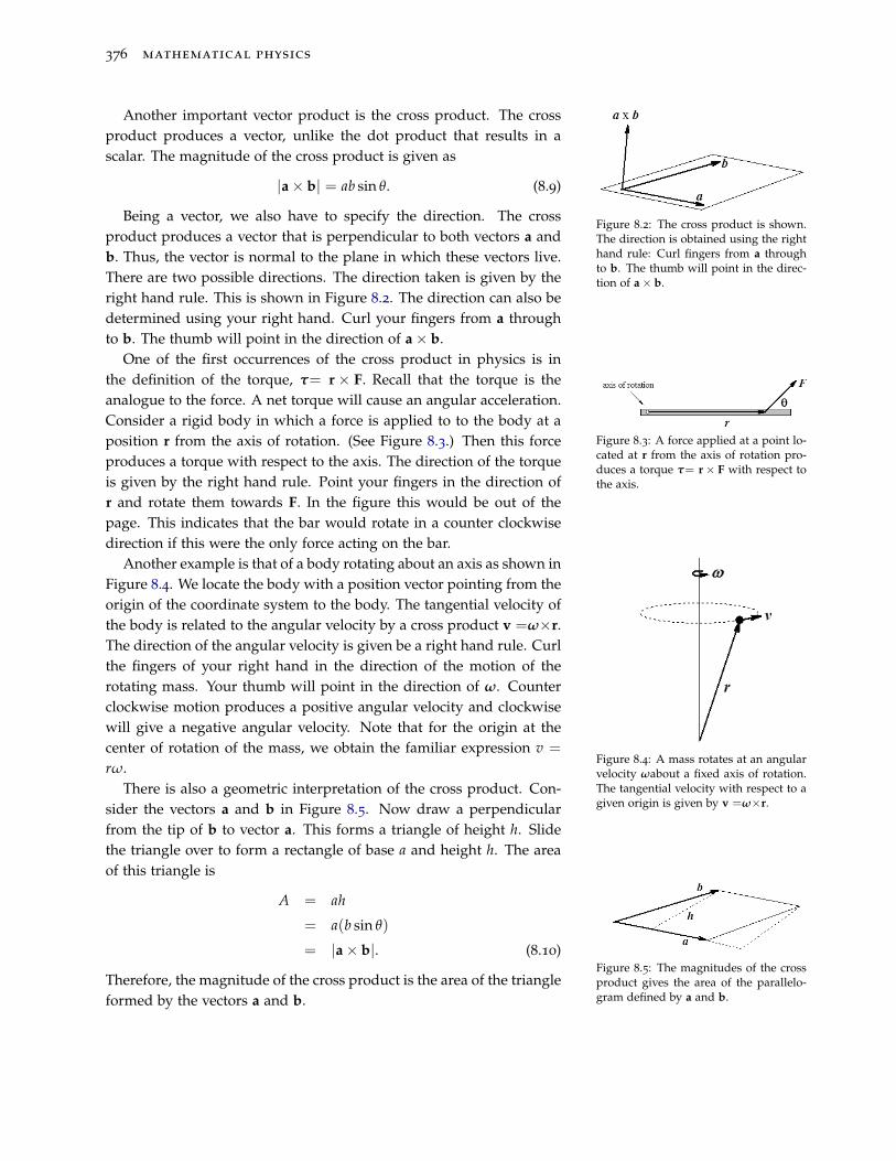
Figure 8.2: The cross product is shown.The direction is obtained using the righthand rule: Curl fingers from a throughto b. The thumb will point in the direc-tion of a× b.
Being a vector, we also have to specify the direction. The crossproduct produces a vector that is perpendicular to both vectors a andb. Thus, the vector is normal to the plane in which these vectors live.There are two possible directions. The direction taken is given by theright hand rule. This is shown in Figure 8.2. The direction can also bedetermined using your right hand. Curl your fingers from a throughto b. The thumb will point in the direction of a× b.
Figure 8.3: A force applied at a point lo-cated at r from the axis of rotation pro-duces a torque τ= r× F with respect tothe axis.
One of the first occurrences of the cross product in physics is inthe definition of the torque, τ= r × F. Recall that the torque is theanalogue to the force. A net torque will cause an angular acceleration.Consider a rigid body in which a force is applied to to the body at aposition r from the axis of rotation. (See Figure 8.3.) Then this forceproduces a torque with respect to the axis. The direction of the torqueis given by the right hand rule. Point your fingers in the direction ofr and rotate them towards F. In the figure this would be out of thepage. This indicates that the bar would rotate in a counter clockwisedirection if this were the only force acting on the bar.
Figure 8.4: A mass rotates at an angularvelocity ωabout a fixed axis of rotation.The tangential velocity with respect to agiven origin is given by v =ω×r.
Another example is that of a body rotating about an axis as shown inFigure 8.4. We locate the body with a position vector pointing from theorigin of the coordinate system to the body. The tangential velocity ofthe body is related to the angular velocity by a cross product v =ω×r.The direction of the angular velocity is given be a right hand rule. Curlthe fingers of your right hand in the direction of the motion of therotating mass. Your thumb will point in the direction of ω. Counterclockwise motion produces a positive angular velocity and clockwisewill give a negative angular velocity. Note that for the origin at thecenter of rotation of the mass, we obtain the familiar expression v =
rω.There is also a geometric interpretation of the cross product. Con-
sider the vectors a and b in Figure 8.5. Now draw a perpendicularfrom the tip of b to vector a. This forms a triangle of height h. Slidethe triangle over to form a rectangle of base a and height h. The areaof this triangle is
A = ah
= a(b sin θ)
= |a× b|. (8.10)
Therefore, the magnitude of the cross product is the area of the triangleformed by the vectors a and b.
Figure 8.5: The magnitudes of the crossproduct gives the area of the parallelo-gram defined by a and b.

vector analysis and em waves 377
The dot product was shown to have a simple form in terms of thecomponents of the vectors. Similarly, we can write the cross productin component form. Recall that we can expand any vector v as
v =n
∑k=1
vkek, (8.11)
where the ek’s are the standard basis vectors.We would like to expand the cross product of two vectors,
u× v =
(n
∑k=1
ukek
)×(
n
∑k=1
vkek
).
In order to do this we need a few properties of the cross product.First of all, the cross product is not commutative. In fact, it is Properties of the cross product.
anticommutative:u× v = −v× u.
A simple consequence of this is that v× v = 0. Just replace u with v inthe anticommutativity rule and you have v× v = −v× v. Somethingthat is its negative must be zero.
The cross product also satisfies distributive properties:
u× (v + w) = u× v + u×w),
andu× (av) = (au)× v = au× v.
Thus, we can expand the cross product in terms of the componentsof the given vectors. A simple computation shows that u× v can beexpressed in terms of sums over ei × ej :
u× v =
(n
∑i=1
uiei
)×(
n
∑j=1
vjej
)
=n
∑i=1
n
∑j=1
uivjei × ej. (8.12)
ij
k
+
ij
k
−
Figure 8.6: The sign for the cross productfor basis vectors can be determined froma simple diagram. Arrange the vectorson a circle as above. If the needed com-putation goes counterclockwise, then thesign is positive. Thus, j × k = i andk× j = −i.
The cross products of basis vectors are simple to compute. First ofall, the cross products ei × ej vanish when i = j by anticommutativityof the cross product. For i 6= j, it is not much more difficult. For thetypical basis, {i, j, k}, this is simple. Imagine computing i × j. Thisis a vector of length |i × j| = |i||j| sin 90◦ = 1. The vector i × j isperpendicular to both vectors, i and j. Thus, the cross product is eitherk or −k. Using the right hand rule, we have i× j = k. Similarly, wefind the following
i× j = k, j× k = i, k× i = j,
j× i = −k, k× j = −i, i× k = −j. (8.13)

378 mathematical physics
Inserting these results into the cross product for vectors in R3, wehave
u× v = (u2v3 − u3v2)i + (u3v1 − u1v3)j + (u1v2 − u2v1)k. (8.14)
While this form for the cross product is correct and useful, there areother forms that help in verifying identities or making computationsimpler with less memorization. However, some of these new expres-sions can lead to problems for the novice as dealing with indices canbe daunting at first sight.
One expression that is useful for computing cross products is thefamiliar computation using determinants. Namely, we have that
u× v =
∣∣∣∣∣∣∣i j k
u1 u2 u3
v1 v2 v3
∣∣∣∣∣∣∣=
∣∣∣∣∣ u2 u3
v2 v3
∣∣∣∣∣ i−∣∣∣∣∣ u1 u3
v1 v3
∣∣∣∣∣ j +
∣∣∣∣∣ u1 u2
v1 v2
∣∣∣∣∣ k
= (u2v3 − u3v2)i + (u3v1 − u1v3)j + (u1v2 − u2v1)k.
(8.15)
A more compact form for the cross product is obtained by introduc-ing the completely antisymmetric symbol, εijk. This symbol is defined The completely antisymmetric symbol,
or permutation symbol, εijk .by the relationsε123 = ε231 = ε312 = 1,
andε321 = ε213 = ε132 = −1,
and all other combinations, like ε113, vanish. Note that all indices mustdiffer. Also, if the order is a cyclic permutation of {1, 2, 3}, then thevalue is +1. For this reason εijk is also called the permutation symbolor the Levi-Civita symbol. We can also indicate the index permutationmore generally using the following identities:
εijk = εjki = εkij = −εjik = −εikj = −εkji.
12
3
+
12
3
−
Figure 8.7: The sign for the permuta-tion symbol can be determined from asimple cyclic diagram similar to that forthe cross product. Arrange the num-bers from 1 to 3 on a circle. If theneeded computation goes counterclock-wise, then the sign is positive, otherwiseit is negative.
Returning to the cross product, we can introduce the standard basise1 = i, e2 = j, and e3 = k. With this notation, we have that
ei × ej =3
∑k=1
εijkek. (8.16)
Example 8.1. Compute the cross product of the basis vectors e2 × e1 usingthe permutation symbol. A straight forward application of the definition ofthe cross product,
e2 × e1 =3
∑k=1
ε21kek
vector analysis and em waves 379
= ε211e1 + ε212e2 + ε213e3
= −e3. (8.17)
It is helpful to write out enough terms in these sums until you get familiarwith manipulating the indices. Note that the first two terms vanished becauseof repeated indices. In the last term we used ε213 = −1.
We now write out the general cross product as
u× v =3
∑i=1
3
∑j=1
uivjei × ej
=3
∑i=1
3
∑j=1
uivj
(3
∑k=1
εijkek
)
=3
∑i,j,k=1
εijkuivjek. (8.18)
Note that the last sum is a triple sum over the indices i, j, and k.
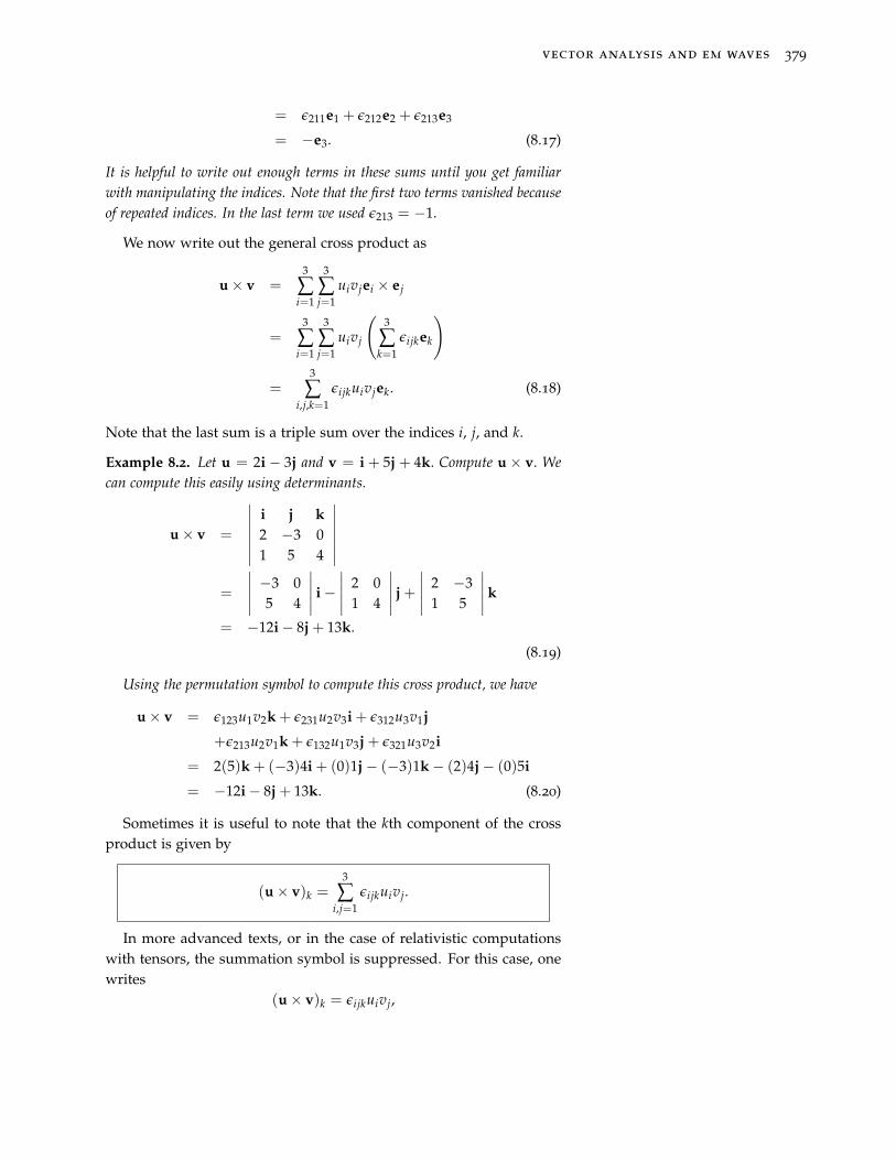
Example 8.2. Let u = 2i− 3j and v = i + 5j + 4k. Compute u× v. Wecan compute this easily using determinants.
u× v =
∣∣∣∣∣∣∣i j k2 −3 01 5 4
∣∣∣∣∣∣∣=
∣∣∣∣∣ −3 05 4
∣∣∣∣∣ i−∣∣∣∣∣ 2 0
1 4
∣∣∣∣∣ j +
∣∣∣∣∣ 2 −31 5
∣∣∣∣∣ k
= −12i− 8j + 13k.
(8.19)
Using the permutation symbol to compute this cross product, we have
u× v = ε123u1v2k + ε231u2v3i + ε312u3v1j
+ε213u2v1k + ε132u1v3j + ε321u3v2i
= 2(5)k + (−3)4i + (0)1j− (−3)1k− (2)4j− (0)5i
= −12i− 8j + 13k. (8.20)
Sometimes it is useful to note that the kth component of the crossproduct is given by
(u× v)k =3
∑i,j=1
εijkuivj.
In more advanced texts, or in the case of relativistic computationswith tensors, the summation symbol is suppressed. For this case, onewrites
(u× v)k = εijkuivj,

380 mathematical physics
where it is understood that summation is performed over repeatedindices. This is called the Einstein summation convention. Einstein summation convention is used
to suppress summation notation. In gen-eral relativity, one also needs to em-ploy raised indices, so that vector com-ponents are written in the form ui . Theconvention then requires that one onlysums over a combination of one lowerand one upper index. Thus, we wouldwrite εijkuivj. We will forgo the need forraised indices.
Since the cross product can be written as both a determinant,
u× v =
∣∣∣∣∣∣∣i j k
u1 u2 u3
v1 v2 v3
∣∣∣∣∣∣∣= εij1uivji + εij2uivjj + εij3uivjk. (8.21)
and using the permutation symbol,
u× v = εijkuivjek,
we can define the determinant as∣∣∣∣∣∣∣a11 a12 a13
a21 a22 a23
a31 a32 a33
∣∣∣∣∣∣∣ =3
∑i,j,k=1
εijka1ia2ja3k. (8.22)
Here we added the triple sum in order to emphasize the hidden sum-mations.
Example 8.3. Compute the determinant
∣∣∣∣∣∣∣1 0 20 −3 42 4 −1
∣∣∣∣∣∣∣ .
We insert the components of each row into the expression for the determi-nant:∣∣∣∣∣∣∣
1 0 20 −3 42 4 −1
∣∣∣∣∣∣∣ = ε123(1)(−3)(−1) + ε231(0)(4)(2) + ε312(2)(0)(4)
+ε213(0)(0)(−1) + ε132(1)(4)(4) + ε321(2)(−3)(2)
= 3 + 0 + 0− 0− 14− (−12)
= 15. (8.23)
Note that if one adds copies of the first two columns, as shown in Fig-ure 8.8, then the products of the first three diagonals, downward to the right(blue), give the positive terms in the determinant computation and the prod-ucts of the last three diagonals, downward to the left (red), give the negativeterms.
1 0 2 1 0
0 -3 4 0 -32 4 -1 2 4
Figure 8.8: Diagram for computing de-terminants.
One useful identity is

vector analysis and em waves 381
εjkiεj`m = δk`δim − δkmδi`,
Product identity satisfied by the permu-tation symbol, εijk .
where δij is the Kronecker delta. Note that the Einstein summationconvention is used in this identity; i.e., summing over j is understood.So, the left side is really a sum of three terms:
εjkiεj`m = ε1kiε1`m + ε2kiε2`m + ε3kiε3`m.
This identity is simple to understand. For nonzero values of theLevi-Civita symbol, we have to require that all indices differ for eachfactor on the left side of the equation: j 6= k 6= i and j 6= ` 6= m. Sincethe first two slots are the same j, and the indices only take values 1, 2,or 3, then either k = ` or k = m. This will give terms with factors of δk`
or δkm. If the former is true, then there is only one possibility for thethird slot, i = m. Thus, we have a term δk`δim. Similarly, the other caseyields the second term on the right side of the identity. We just needto get the signs right. Obviously, changing the order of ` and m willintroduce a minus sign. A little care will show that the identity givesthe correct ordering.
Other identities involving the permutation symbol are
εmjkεnjk = 2δmn,
εijkεijk = 6.
We will end this section by recalling triple products. There are onlytwo ways to construct triple products. Starting with the cross productb× c, which is a vector, we can multiply the cross product by a a toeither obtain a scalar or a vector.
In the first case we have the triple scalar product, a · (b× c). Actu-ally, we do not need the parentheses. Writing a ·b× c could only meanone thing. If we computed a · b first, we would get a scalar. Then theresult would be a multiple of c, which is not a scalar. So, leaving offthe parentheses would mean that we want the triple scalar product byconvention.
Let’s consider the component form of this product. We will usethe Einstein summation convention and the fact that the permutationsymbol is cyclic in ijk. Using εjki = εijk,
a · (b× c) = ai(b× c)i
= εjkiaibjck
= εijkaibjck
= (a× b)kck
= (a× b) · c. (8.24)
We have proven that
a · (b× c) = (a× b) · c.
382 mathematical physics
Now, imagine how much writing would be involved if we had ex-panded everything out in terms of all of the components.
Note that this result suggests that the triple scalar product can becomputed by just computing a determinant:
a · (b× c) = εijkaibjck
=
∣∣∣∣∣∣∣a1 a2 a3
b1 b2 b3
c1 c2 c3
∣∣∣∣∣∣∣ . (8.25)
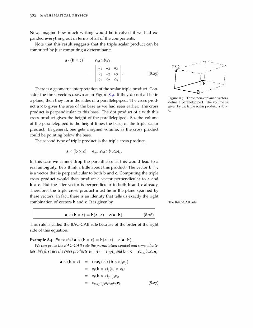
Figure 8.9: Three non-coplanar vectorsdefine a parallelepiped. The volume isgiven by the triple scalar product, a · b×c.
There is a geometric interpretation of the scalar triple product. Con-sider the three vectors drawn as in Figure 8.9. If they do not all lie ina plane, then they form the sides of a parallelepiped. The cross prod-uct a× b gives the area of the base as we had seen earlier. The crossproduct is perpendicular to this base. The dot product of c with thiscross product gives the height of the parallelepiped. So, the volumeof the parallelepiped is the height times the base, or the triple scalarproduct. In general, one gets a signed volume, as the cross productcould be pointing below the base.
The second type of triple product is the triple cross product,
a× (b× c) = εmnjεijkaibmcnek.
In this case we cannot drop the parentheses as this would lead to areal ambiguity. Lets think a little about this product. The vector b× cis a vector that is perpendicular to both b and c. Computing the triplecross product would then produce a vector perpendicular to a andb × c. But the later vector is perpendicular to both b and c already.Therefore, the triple cross product must lie in the plane spanned bythese vectors. In fact, there is an identity that tells us exactly the rightcombination of vectors b and c. It is given by The BAC-CAB rule.
a× (b× c) = b(a · c)− c(a · b). (8.26)
This rule is called the BAC-CAB rule because of the order of the rightside of this equation.
Example 8.4. Prove that a× (b× c) = b(a · c)− c(a · b).We can prove the BAC-CAB rule the permutation symbol and some identi-
ties. We first use the cross products ei× ej = εijkek and b× c = εmnjbmcnej :
a× (b× c) = (aiei)× ((b× c)jej)
= ai(b× c)j(ei × ej)
= ai(b× c)jεijkek
= εmnjεijkaibmcnek (8.27)

vector analysis and em waves 383
Now, we use the identity
εmnjεijk = δmkδni − δmiδnk,
the properties of the Kronecker delta functions, and then rearrange the resultsto finish the proof:
a× (b× c) = εmnjεijkaibmcnek
= aibmcn (δmkδni − δmiδnk) ek
= anbmcnem − ambmcnen
= (bmem)(cnan)− (cnen)(ambm)
= b(a · c)− c(a · b). (8.28)
8.1.2 Differentiation and Integration of Vectors
You have already been introduced to the idea that vectors canbe differentiated and integrated in your introductory physics course.These ideas are also the major theme encountered in a multivariate cal-culus class, or Calculus III. We review some of these topics in the nextsections. We first recall the differentiation and integration of vectorfunctions.
v(t)
r(t)
O
Figure 8.10: Position and velocity vectorsof moving particle.
The position vector can change in time, r(t) = x(t)i + y(t)j + x(t)k.The rate of change of this vector is the velocity,
v(t) =drdt
= lim∆t→0
r(t + ∆t)− r(t)∆t
=dxdt
i +dydt
j +dzdt
k
= vxi + vyk + vzk. (8.29)
The velocity vector is tangent to the path, r(t), as seen in Figure 8.1.2.The magnitude of this vector gives the speed,
|v| =
√(dxdt
)2+
(dydt
)2+
(dzdt
)2.
Moreover, differentiating this vector gives the acceleration, a(t) =
v′(t).In general, one can differentiate an arbitrary time-dependent vector
v(t) = f (t)i + g(t)j + h(t)k as
dvdt
=d fdt
i +dgdt
j +dhdt
k. (8.30)

384 mathematical physics
Example 8.5. A simple example is given by the motion on a circle. A circlein the xy-plane can be parametrized as r(t) = r cos(ωt)i + r sin(ωt)j. Thenthe velocity is found as
v(t) = −rω sin(ωt)i + rω cos(ωt)j.
Its speed is v = rω, which is easily recognized as the tangential speed. Theacceleration is
a(t) = −ω2r cos(ωt)i−ω2r sin(ωt)j.
The magnitude gives the centripetal acceleration, a = ω2r and the accelera-tion vector is pointing towards the center of the circle.
v(t)
r(t)O
Figure 8.11: Particle on circular path.
Once one can differentiate time-dependent vectors, one can provesome standard properties.
a.ddt
[u + v] =dudt
+dvdt
.
b.ddt
[cu] = cdudt
.
c.ddt
[ f (t)u] = f ′(t)u + f (t)dudt
.
d.ddt
[u · v] = dudt· v + u · dv
dt.
e.ddt
[u× v] =dudt× v + u× dv
dt.
f.ddt
[u( f (t))] =dud f
d fdt
.
Example 8.6. Let |r(t)| =const. Then, r′(t) is perpendicular r(t).Since |r| =const, |r|2 = r · r =const. Differentiating this expression, one
has ddt (r · r) = 2r · dr
dt = 0. Therefore, r · drdt = 0, as was to be shown.
In this discussion, we have referred to t as the time. However, whenparametrizing spacecurves, t could represent any parameter. For ex-ample, the circle could be parametrized for t the angle swept out alongany arc of the circle, r(t) = r cos ti + r sin tj, for t1 ≤ t ≤ t2. We canstill differentiate with respect to this parameter. It not longer has themeaning of velocity. another standard parameter is that of arclength.The arclength of a path is the distance along the path from some start-ing point. In deriving an expression for arclength, one first considersincremental distances along paths. Moving from point (x, y, z) to point(x + ∆x, y + ∆y, z + ∆z), one has gone a distance of
∆s =√(∆x)2 + (∆y)2 + (∆z)2.
Given a curve parametrized by t, such as the time, one can rewrite thisas
∆s =
√(∆x∆t
)2+
(∆y∆t
)2+
(∆z∆t
)2∆t.

vector analysis and em waves 385
Letting ∆t get small, as well as the other increments, we are led to
ds =
√(dxdt
)2+
(dydt
)2+
(dzdt
)2dt. (8.31)
We note that the square root is |r′(t)|. So,
ds = |r′(t)|dt,
ordsdt
= |r′(t)|.
In order to find the total arclength, we need only integrate over theparameter range,
s =∫ t2
t1
|r′(t)| dt.
If t is time and r(t) is the position vector of a particle, then |r′(t)| isthe particle speed and we have that the distance traveled is simply anintegral of the speed,
s =∫ t2
t1
v dt.
If one is interested in knowing the distance traveled from point r(t1)
to an arbitrary point r(t), one can define the arclength function
s(t) =∫ t
t1
|r′(τ)| dτ.
Example 8.7. Determine the length of the parabolic path described by r =
ti + t2j, t ∈ [0, 1].We want to determine the length, L =
∫ 10 |r′(t)| dt, of a path. First, we
have r′(t) = i + 2tj. Then, |r′(t)| =√
1 + 4t2. Using∫ √t2 + a2 dt =
12
(t√
t2 + a2 + a2 ln(t +√
t2 + a2))
,
s =∫ 1
0|r′(t)| dt
=∫ 1
0
√1 + 4t2 dt
=
[x
√x2 +
14+
14
ln
(x +
√x2 +
14
)]1
0
=
√5
2+
14
ln(2 +√
5). (8.32)
Line integrals are defined as integrals of functions along a path, orcurve, in space. Let f (x, y, z) be the function, and C a parametrized
386 mathematical physics
path. Then we are interested in computing∫
C f (x, y, z) ds, where sis the arclength parameter. This integral looks similar to the contourintegrals that we had studied in Chapter 5. We can compute suchintegrals in a similar manner by introducing the parametrization:∫
Cf (x, y, z) ds =
∫C
f (x(t), y(t), z(t))|r′(t)| dt.
Example 8.8. Compute∫
C(x2 + y2 + z2) ds for the helical path r = (cos t, sin t, t),t ∈ [0, 2π].
In order to do this integral, we have to integrate over the given range of tvalues. So, we replace ds with |r′(t)|dt. In this problem |r′(t)| =
√2. Also,
we insert the parametric forms for x(t) = cos t, y(t) = sin t, and z = t intof (x, y, z). Thus,
∫C(x2 + y2 + z2) ds =
∫ 2π
0(1 + t2)
√2 dt = 2
√2π
(1 +
4π2
3
). (8.33)
One can also integrate vector functions. Given the vector functionv(t) = f (t)i+ g(t)j+ h(t)k, we can do a straight forward term by termintegration,
∫ b
av(t) dt =
∫ b
af (t) dti +
∫ b
ag(t) dtj +
∫ b
ah(t) dtk.
If v(t) is the velocity and t is the time, then
∫ b
av(t) dt =
∫ b
a
drdt
dt = r(b)− r(a).
We can thus interpret this integral as giving the displacement of aparticle between times t = a and t = b.
At the beginning of this chapter we had recalled the work done ona body by a nonconstant force F over a path C,
W =∫
CF · dr (8.34)
If the path is parametrized by t, then we can write dr = drdt dt. Thus the
prescription for computing line integrals such as this is
∫C
F · dr =∫
CF · dr
dtdt.
There are other forms that such line integrals can take. Let F =
P(x, y, z)i + Q(x, y, z)j + R(x, y, z)k. Noting that dr = dxi + dyy + dzk,then we can write∫
CF · dr =
∫C
P(x, y, z) dx + Q(x, y, z) dy + R(x, y, z) dz.

vector analysis and em waves 387
Example 8.9. Compute the work done by the force F = yi− xj on a particleas it moves around the circle r = (cos t)i + (sin t)j, for 0 ≤ t ≤ π.
W =∫
CF · dr =
∫C
y dx− x dy.
One way to complete this is to note that dx = − sin t dt and dy = cos t dt.Then ∫
Cy dx− x dy =
∫ π
0(− sin2 t− cos2 t) dt = −π.
8.1.3 Div, Grad, Curl
Throughout physics we see functions which vary in both spaceand time. A function f (x, y, z, t) is called a scalar function when theoutput is a scalar, or number. An example of such a function is thetemperature. A function F(x, y, z, t) is called a vector (or vector val-ued) function if the output of the function is a vector. Let v(x, y, z, t)represent the velocity of a fluid at position (x, y, z) at time t. This is anexample of a vector function. Typically when we assign a number, or avector, to every point in a domain, we refer to this as a scalar, or vector,field. In this section we discuss how fields change from one point inspace to another. Namely, we look at derivatives of multivariate func-tions with respect to their independent variables and the meanings ofthese derivatives in a physical context.
In studying functions of one variable in calculus, one is introducedto the derivative, d f
dx : The derivative has several meanings. The stan-dard mathematical meaning is that the derivative gives the slope ofthe graph of f (x) at x. The derivative also tells us how rapidly f (x)varies when x is changed by dx. Recall that dx is called a differential.We can think of the differential dx as an infinitesimal increment in x.Then changing x by an amount dx results in a change in f (x) by
d f =d fdx
dx.
We can extend this idea to functions of several variables. Considerthe temperature T(x, y, z) at a point in space. The change in tempera-ture depends on the direction in which one moves in space. Extendingthe above relation between differentials of the dependent and indepen-dent variables, we have
dT =∂T∂x
dx +∂T∂y
dy +∂T∂z
dz. (8.35)
Note that if we only changed x, keeping y and z fixed, then we recoverthe form dT = dT
dx dx.

388 mathematical physics
Introducing the vectors,
dr = dxi + dyj + dzk, (8.36)
The gradient of a function,
∇T =∂T∂x
i +∂T∂y
j +∂T∂z
k, .∇T ≡ ∂T
∂xi +
∂T∂y
j +∂T∂z
k, (8.37)
we can write Equation (8.35) as
dT = ∇T · dr (8.38)
Equation (8.37) defines the gradient of a scalar function, T. Equation(8.38) gives the change in T as one moves in the direction dr.
Using the definition of the dot product, we also have
dT = |∇T||dr| cos θ.
Note that by fixing |dr| and varying θ, the maximum value of dT isobtained when cos θ = 1. Thus, the maximum value of dT is in thedirection of the gradient. Similarly, since cos π = −1, the minimumvalue of dT is in a direction 180◦ from the gradient. The greatest change is a function is in the
direction of its gradient.Example 8.10. Let f (x, y, z) = x2y + zexy. Compute ∇ f .
∇ f =∂ f∂x
i +∂ f∂y
j +∂ f∂z
k,
= (2xy + yzexy)i + (x2 + xzexy)j + exyk. (8.39)
From this analysis, we see that the rate of change of a function, suchas T(x, y, z, ), depends on the direction one heads away from a givenpoint. So, if one moves an infinitesimal distance ds in some directiondr, then how does T change with respect to s? Another way to askthis is to ask what is the directional derivative of T in direction n? Wedefine this directional derivative as The directional derivative of a function,
DnT = dTds = ∇T · n.
DnT =dTds
. (8.40)
We can develop an operational definition of the directional deriva-tive. From Equation (8.38) we have
dTds
= ∇T · drds
. (8.41)
We note thatdrds
=
(dxds
)i +(
dyds
)j +(
dzds
)k
and ∣∣∣∣drds
∣∣∣∣ =√(
dxds
)2+
(dyds
)2+
(dzds
)2= 1.
Thus, n = drds is a unit vector pointing in the direction of interest and
the directional derivative of T(x, y, z) in direction n can be written as
DnT = ∇T · n. (8.42)
vector analysis and em waves 389
Example 8.11. Let the temperature in a rectangular plate be given by T(x, y) =5.0 sin 3πx
2 sin πy2 . Determine the directional derivative at (x, y) = (1, 1) in
the following directions: (a) i, (b) 3i + 4j.In part (a) we have
DiT = ∇T · i = ∂T∂x
.
So,
DiT∣∣∣∣(1,1)
=152
cos3π
2sin
π
2= 0.
In part (b) the direction given is not a unit vector, |3i + 4j| = 5. Dividingby the length of the vector, we obtain a unit normal vector, n = 3
5 i + 45 j. The
directional derivative can now be computed:
DnT = ∇T · n
=35
∂T∂x
+45
∂T∂y
=9π
2cos
3πx2
sinπy2
+ 2π sin3πx
2cos
πy2
. (8.43)
Evaluating this result at (x, y) = (1, 1), we have
DnT∣∣∣∣(1,1)
=9π
2cos
3π
2sin
π
2+ 2π sin
3π
2cos
π
2= 0.
We can write the gradient in the form
∇T =
(∂
∂xi +
∂
∂yj +
∂
∂zk)
T. (8.44)
Thus, we see that the gradient can be viewed as an operator acting onT. The operator,
∇ =∂
∂xi +
∂
∂yj +
∂
∂zk,
is called the del, or gradient, operator. It is a differential vector operator.It can act on scalar functions to produce a vector field. Recall, if thegravitational potential is given by Φ(r), then the gravitational force isfound as F = −∇Φ.
We can also allow the del operator to act on vector fields. Recallthat a vector field is simply a vector valued function. For example, aforce field is a function defined at points in space indicating the forcethat would act on a mass placed at that location. We could denote it asF(x, y, z). Again, think about the gravitational force above. The forceacting on a mass in the Earth’s gravitational field is a given by a vectorfield. At each point in space one would see that the force vector takeson different magnitudes and directions depending upon the locationof the mass in space.
How can we combine the (vector) del operator and a vector field?Well, we could “multiply” them. We could either compute the dot

390 mathematical physics
product, ∇ · F, or we could compute the cross product ∇× F. The firstexpression is called the divergence of the vector field and the second iscalled the curl of the vector field. These are typically encountered in athird semester calculus course. In some texts they are denoted by divF and curl F.
The divergence is computed the same as any other dot product. The divergence, div F = ∇ · F.
Writing the vector field in component form,
F = F1(x, y, z)i + F2(x, y, z)j + F3(x, y, z)k,
we find the divergence is simply given as
∇ · F =
(∂
∂xi +
∂
∂yj +
∂
∂zk)· (F1i + F2j + F3k)
=∂F1
∂x+
∂F2
∂y+
∂F3
∂z(8.45)
Similarly, we can compute the curl of F. Using the determinant The curl F = ∇× F.
form, we have
∇× F =
(∂
∂xi +
∂
∂yj +
∂
∂zk)× (F1i + F2j + F3k)
=
∣∣∣∣∣∣∣i j k∂
∂x∂
∂y∂
∂y
F1 F2 F3
∣∣∣∣∣∣∣=
(∂F3
∂y− ∂F2
∂z
)i +(
∂F1
∂z− ∂F3
∂x
)j +(
∂F2
∂x− ∂F1
∂y
)k.
(8.46)
Example 8.12. Compute the divergence and curl of the vector field: F =
yi− xj.
∇ · F =∂y∂x− ∂x
∂y= 0.
∇× F =
∣∣∣∣∣∣∣i j k∂
∂x∂
∂y∂
∂y
y −x 0
∣∣∣∣∣∣∣=
(−∂x
∂x− ∂y
∂y
)k = −2. (8.47)
These operations also have interpretations. The divergence mea-sures how much the vector field F spreads from a point. When thedivergence of a vector field is nonzero around a point, that is an in-dication that there is a source (div F > 0) or a sink (div F < 0). Forexample, ∇ · E = ρ
ε0indicates that there are sources contributing to the
electric rled. For a single charge, the field lines are radially pointing

vector analysis and em waves 391
towards (sink) or away from (source) the charge. A field in which thedivergence is zero is called divergenceless or solenoidal.
The curl is an indication of a rotational field. It is a measure of howmuch a field curls around a point. Consider the flow of a stream. Thevelocity of each element of fluid can be represented by a velocity field.If the curl of the field is nonzero, then when we drop a leaf into thestream we will see it begin to rotate about some point. A field that haszero curl is called irrotational.
The last common differential operator is the Laplace operator. This The Laplace operator, ∇2 f = ∂2 f∂x2 +
∂2 f∂y2 + ∂2 f
∂z2 .is the common second derivative operator, the divergence of the gra-dient,
∇2 f = ∇ · ∇ f .
It is easily computed as
∇2 f = ∇ · ∇ f
= ∇ ·(
∂ f∂x
i +∂ f∂y
j +∂ f∂z
k)
=∂2 f∂x2 +
∂2 f∂y2 +
∂2 f∂z2 . (8.48)
8.1.4 The Integral Theorems
Maxwell’s equations are given later in this chapter in dif-ferential form and only describe electric and magnetic fields locally.At times we would like to also provide global information, or informa-tion over an finite region. In this case one can derive various integraltheorems. These are the finale in a three semester calculus sequence.We will not delve into these theorems here, as this will take us awayfrom our goal of deriving a three dimensional wave equation. How-ever, these integral theorems are important and useful in deriving localconservation laws.
These theorems are all different versions of a generalized Funda-mental Theorem of Calculus:
(a)∫ b
ad fdx dx = f (b)− f (a), The Fundamental Theorem of
Calculus in 1D.
(b)∫ b
a ∇T · dr = T(b)− T(a), The Fundamental Theoremof Calculus for Vector Fields.
(c)∮
C (P dx + Q dy) =∫
D
(∂Q∂x −
∂P∂y
)dxdy, Green’s Theo-
rem in the Plane.
(d)∫
V ∇ · F dV =∮
S F · da, Gauss’ Divergence Theorem.
(e)∫
S(∇× F) · da =∮
C F · dr, Stoke’s Theorem.
392 mathematical physics
The connections between these integral theorems are probably moreeasily seen by thinking in terms of fluids. Consider a fluid with massdensity ρ(x, y, z) and fluid velocity v(x, y, z, t). We define (Q) = ρv asthe mass flow rate. [Note the units are kg/m2/s indicating the massper area per time.]
Now consider the fluid flowing through an imaginary rectangularbox. Let the fluid flow into the left face and out the right face. Therate at which the fluid mass flows through a face can be representedby Q · dσ, where dσ = ndσ represents the differential area elementnormal to the face. The rate of flow across the left face is
Q · dσ = −Qy dxdz∣∣∣y
and that flowing across the right face is
Q · dσ = Qy dxdz∣∣∣y+dy
.
The net flow rate is the sum of these
Qydxdz∣∣∣y+dy−Qydxdz
∣∣∣y=
∂Qy
∂ydxdydz.
A similar computation can be done for the other faces, leading tothe result that the total rate of flow is ∇ ·Q dτ, where dτ = dxdydz isthe volume element. So, the rate of flow per volume from the volumeelement gives
∇ ·Q = −∂ρ
∂t.
Note that if more fluid is flowing out the right face than is flowing into Conservation of mass equation,
∂ρ
∂t+∇ ·Q = 0.
the left face, then the amount of fluid inside the region will decrease.That is why the right hand side of this equation has the negative sign.
If the fluid is incompressible, i.e., ρ =const., then ∇ ·Q = 0, whichimplies ∇ · v = 0 assuming there are no sinks or sources. If therewere a sink in the rectangular box, then there would be a loss of fluidnot accounted for. Likewise, is a hose were inserted and fluid weresupplied, then one would have a source.
If there are sinks, or sources, then the net mass due to these wouldcontribute to an overall flow through the surrounding surface. This iscaptured by the equation Gauss’ Divergence Theorem∫
V∇ ·Q dτ︸ ︷︷ ︸
Net mass due to sink/sources
=∮
SQ · n dσ︸ ︷︷ ︸
Net flow outward from S
. (8.49)
Dividing out the constant mass density, since Q = ρv, this becomes
∫V∇ · v dτ =
∮S
v · n dσ. (8.50)

vector analysis and em waves 393
The surface integral on the right had side is called the flux of the vectorfield through surface S. This is nothing other than Gauss’ DivergenceTheorem.1 1 We should note that the Divergence
Theorem holds provided v is a continu-ous vector field and has continuous par-tial derivatives in a domain containingV. Also, n is the outward normal to thesurface S.
The unit normal can be written in terms of the direction cosines,
n = cos αi + cos βj + cos γk,
where the angles are the directions between n and the coordinate axes.For example, n · i = cos α. For vector v = v1i + v2j + v3k, we have∫
Sv · n dσ =
∫S(v1 cos α + v2 cos β + v3 cos γ) dσ
=∫
S(u1dydz + u2dzdx + u3dxdy). (8.51)
Example 8.13. Use the Divergence Theorem to compute∫S(x2dydz + y2dzdx + z2dxdy)
for S the surface of the unit cube, [0, 1]× [0, 1]× [0, 1].We first compute the divergence of the vector v = x2i + y2j + z2k, which
we obtained from the coefficients in the given integral. Then
∇ · v =∂x2
∂x+
∂y2
∂y+
∂z2
∂z= 2(x + y + z).
Then,∫S(x2dydz + y2dzdx + z2dxdy) =
∫V
2(x + y + z) dτ
= 2∫ 1
0
∫ 1
0
∫ 1
0(x + y + z) dxdydz
= 2∫ 1
0
∫ 1
0(
12+ y + z) dydz
= 2∫ 1
0(
12+
12+ z) dz
= 2(1 +12) = 3. (8.52)
The other integral theorem’s are just a variation of the divergencetheorem. For example, a two dimensional version of this obtainedby considering a simply connected region, D, bounded by a simpleclosed curve, C. One could think of the laminar flow of a thin sheet offluid. Then the total mass in contained in D and the net mass would berelated to the next flow through the boundary, C. The integral theoremfor this situation is given as∫
D∇ · v dA =
∮C
v · n ds. (8.53)
The tangent vector to the curve at point r on the curve C, is
drds
=dxds
i +dyds
j.
394 mathematical physics
Therefore, the outward normal at that point is given by
n =dyds
i− dxds
j.
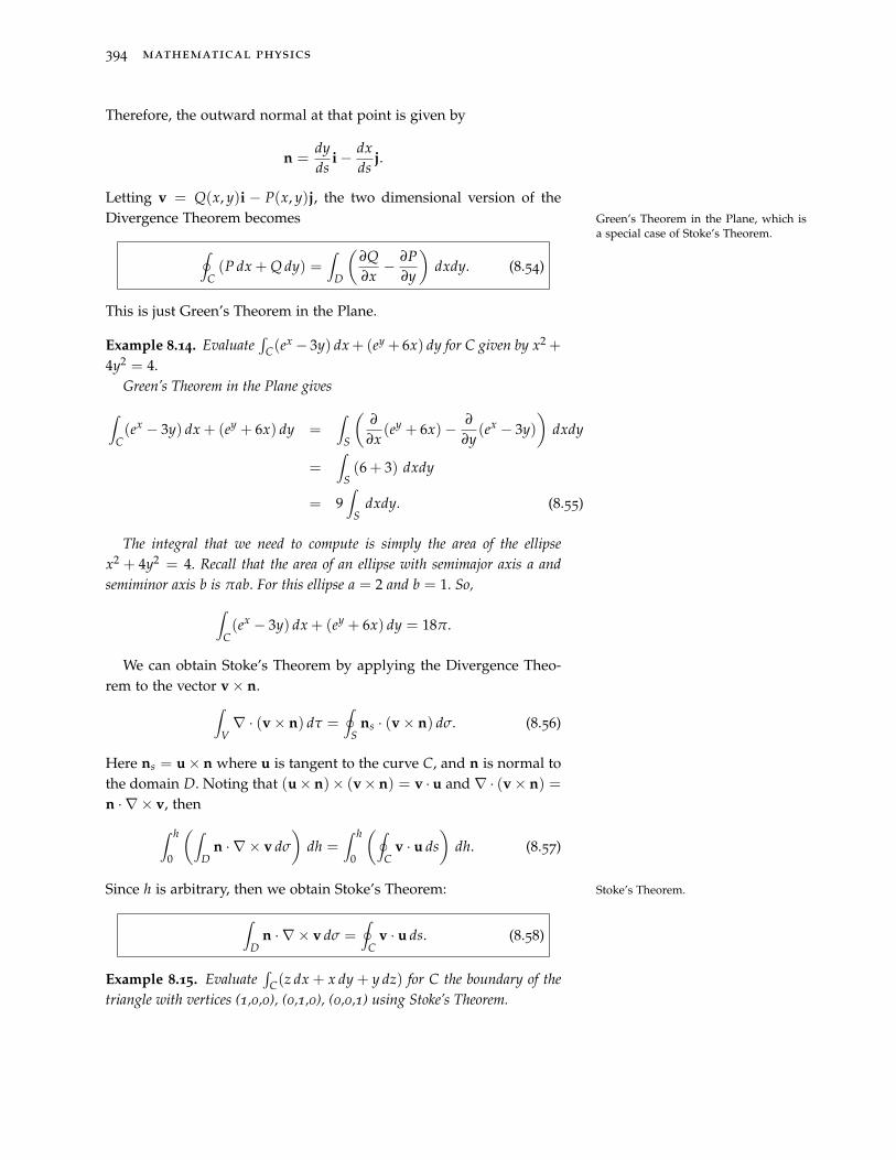
Letting v = Q(x, y)i − P(x, y)j, the two dimensional version of theDivergence Theorem becomes Green’s Theorem in the Plane, which is
a special case of Stoke’s Theorem.∮C(P dx + Q dy) =
∫D
(∂Q∂x− ∂P
∂y
)dxdy. (8.54)
This is just Green’s Theorem in the Plane.
Example 8.14. Evaluate∫
C(ex − 3y) dx + (ey + 6x) dy for C given by x2 +
4y2 = 4.Green’s Theorem in the Plane gives
∫C(ex − 3y) dx + (ey + 6x) dy =
∫S
(∂
∂x(ey + 6x)− ∂
∂y(ex − 3y)
)dxdy
=∫
S(6 + 3) dxdy
= 9∫
Sdxdy. (8.55)
The integral that we need to compute is simply the area of the ellipsex2 + 4y2 = 4. Recall that the area of an ellipse with semimajor axis a andsemiminor axis b is πab. For this ellipse a = 2 and b = 1. So,∫
C(ex − 3y) dx + (ey + 6x) dy = 18π.
We can obtain Stoke’s Theorem by applying the Divergence Theo-rem to the vector v× n.∫
V∇ · (v× n) dτ =
∮S
ns · (v× n) dσ. (8.56)
Here ns = u× n where u is tangent to the curve C, and n is normal tothe domain D. Noting that (u× n)× (v× n) = v · u and ∇ · (v× n) =n · ∇ × v, then∫ h
0
(∫D
n · ∇ × v dσ
)dh =
∫ h
0
(∮C
v · u ds)
dh. (8.57)
Since h is arbitrary, then we obtain Stoke’s Theorem: Stoke’s Theorem.
∫D
n · ∇ × v dσ =∮
Cv · u ds. (8.58)
Example 8.15. Evaluate∫
C(z dx + x dy + y dz) for C the boundary of thetriangle with vertices (1,0,0), (0,1,0), (0,0,1) using Stoke’s Theorem.
vector analysis and em waves 395
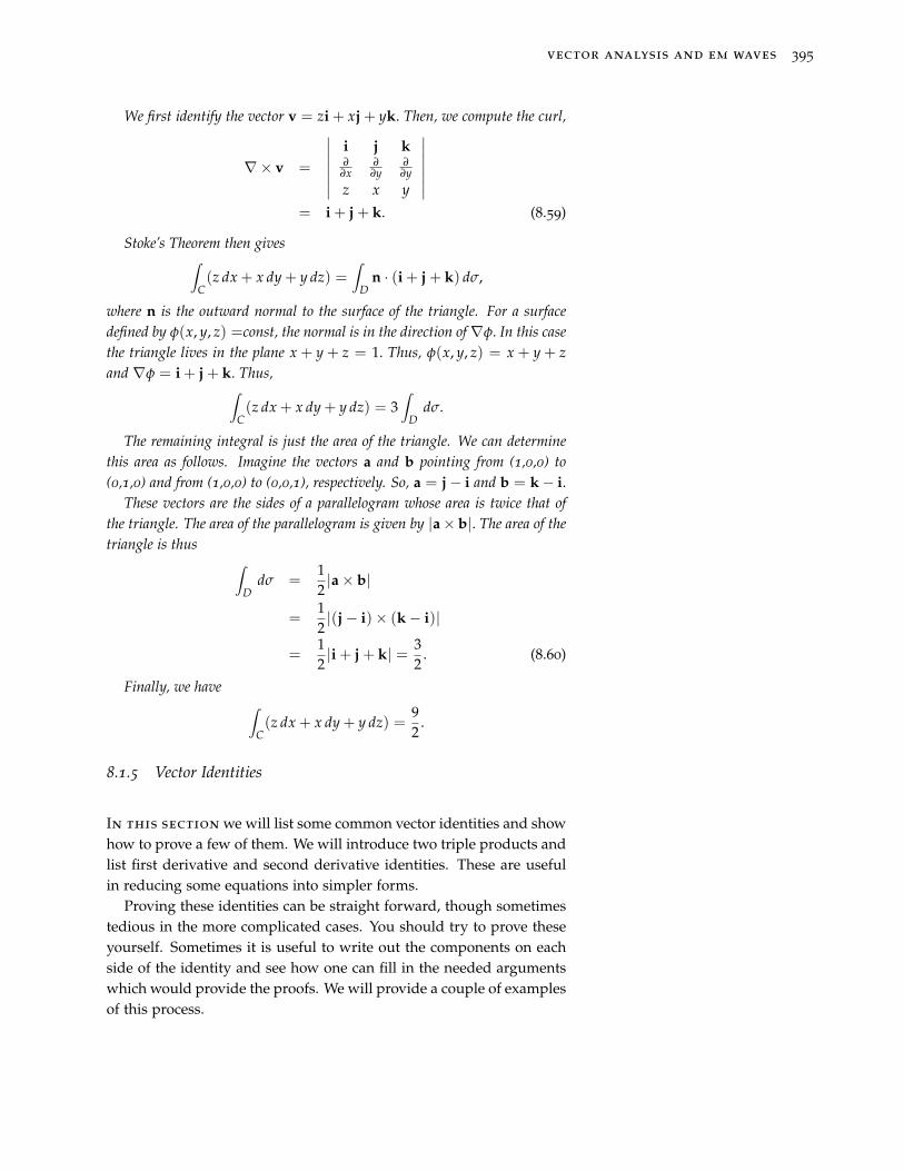
We first identify the vector v = zi + xj + yk. Then, we compute the curl,
∇× v =
∣∣∣∣∣∣∣i j k∂
∂x∂
∂y∂
∂y
z x y
∣∣∣∣∣∣∣= i + j + k. (8.59)
Stoke’s Theorem then gives∫C(z dx + x dy + y dz) =
∫D
n · (i + j + k) dσ,
where n is the outward normal to the surface of the triangle. For a surfacedefined by φ(x, y, z) =const, the normal is in the direction of∇φ. In this casethe triangle lives in the plane x + y + z = 1. Thus, φ(x, y, z) = x + y + zand ∇φ = i + j + k. Thus,∫
C(z dx + x dy + y dz) = 3
∫D
dσ.
The remaining integral is just the area of the triangle. We can determinethis area as follows. Imagine the vectors a and b pointing from (1,0,0) to(0,1,0) and from (1,0,0) to (0,0,1), respectively. So, a = j− i and b = k− i.
These vectors are the sides of a parallelogram whose area is twice that ofthe triangle. The area of the parallelogram is given by |a× b|. The area of thetriangle is thus ∫
Ddσ =
12|a× b|
=12|(j− i)× (k− i)|
=12|i + j + k| = 3
2. (8.60)
Finally, we have ∫C(z dx + x dy + y dz) =
92
.
8.1.5 Vector Identities
In this section we will list some common vector identities and showhow to prove a few of them. We will introduce two triple products andlist first derivative and second derivative identities. These are usefulin reducing some equations into simpler forms.
Proving these identities can be straight forward, though sometimestedious in the more complicated cases. You should try to prove theseyourself. Sometimes it is useful to write out the components on eachside of the identity and see how one can fill in the needed argumentswhich would provide the proofs. We will provide a couple of examplesof this process.
396 mathematical physics
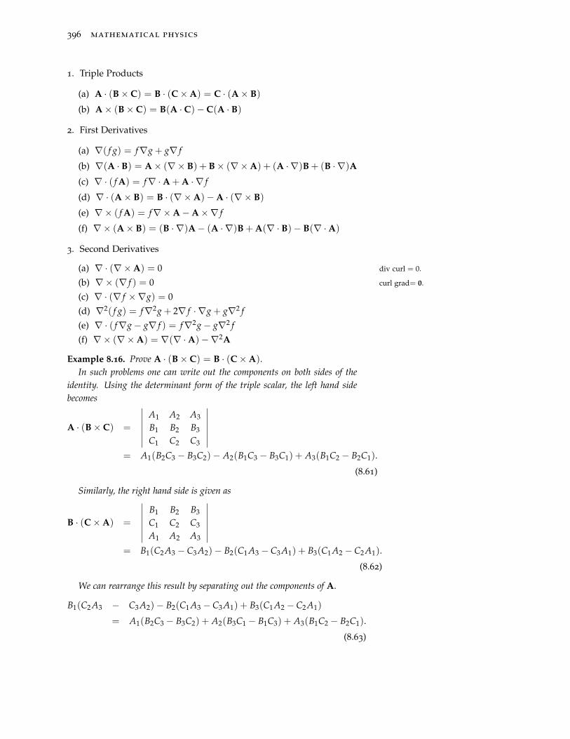
1. Triple Products
(a) A · (B× C) = B · (C×A) = C · (A× B)
(b) A× (B× C) = B(A · C)− C(A · B)
2. First Derivatives
(a) ∇( f g) = f∇g + g∇ f
(b) ∇(A · B) = A× (∇× B) + B× (∇×A) + (A · ∇)B + (B · ∇)A(c) ∇ · ( f A) = f∇ ·A + A · ∇ f
(d) ∇ · (A× B) = B · (∇×A)−A · (∇× B)
(e) ∇× ( f A) = f∇×A−A×∇ f
(f) ∇× (A× B) = (B · ∇)A− (A · ∇)B + A(∇ · B)− B(∇ ·A)
3. Second Derivatives
(a) ∇ · (∇×A) = 0 div curl = 0.
(b) ∇× (∇ f ) = 0 curl grad= 0.
(c) ∇ · (∇ f ×∇g) = 0
(d) ∇2( f g) = f∇2g + 2∇ f · ∇g + g∇2 f(e) ∇ · ( f∇g− g∇ f ) = f∇2g− g∇2 f(f) ∇× (∇×A) = ∇(∇ ·A)−∇2A
Example 8.16. Prove A · (B× C) = B · (C×A).In such problems one can write out the components on both sides of the
identity. Using the determinant form of the triple scalar, the left hand sidebecomes
A · (B× C) =
∣∣∣∣∣∣∣A1 A2 A3
B1 B2 B3
C1 C2 C3
∣∣∣∣∣∣∣= A1(B2C3 − B3C2)− A2(B1C3 − B3C1) + A3(B1C2 − B2C1).
(8.61)
Similarly, the right hand side is given as
B · (C×A) =
∣∣∣∣∣∣∣B1 B2 B3
C1 C2 C3
A1 A2 A3
∣∣∣∣∣∣∣= B1(C2 A3 − C3 A2)− B2(C1 A3 − C3 A1) + B3(C1 A2 − C2 A1).
(8.62)
We can rearrange this result by separating out the components of A.
B1(C2 A3 − C3 A2)− B2(C1 A3 − C3 A1) + B3(C1 A2 − C2 A1)
= A1(B2C3 − B3C2) + A2(B3C1 − B1C3) + A3(B1C2 − B2C1).
(8.63)

vector analysis and em waves 397
Upon inspection, we see that we obtain the same result as we had for the lefthand side.
This problem can also be solved using the completely antisymmetric sym-bol, εijk. Recall that the scalar triple product is given by
A · (B× C) = εijk AiBjCk.
(We have employed the Einstein summation convention.) Since εijk = εjki,we have
εijk AiBjCk = εjki AiBjCk = εjkiBjCk Ai.
But,εjkiBjCk Ai = B · (C×A).
So, we have once again proven the identity. However, it took a little less workand an understanding of the antisymmetric symbol. Furthermore, you shouldnote that this identity was proven earlier in the chapter.
Example 8.17. Prove∇( f g) = f∇g + g∇ f . In this problem we compte thegradient of f g. Then we note that each derivative is the derivative of a productand apply the Product Rule. Carefully writing out the terms, we obtain thedesired result.
∇( f g) =∂ f g∂x
i +∂ f g∂y
j +∂ f g∂z
k
=
(∂ f∂x
i +∂ f∂y
j +∂ f∂z
k)
g + f(
∂g∂x
i +∂g∂y
j +∂g∂z
k)
= f∇g + g∇ f . (8.64)
8.2 Electromagnetic Waves
8.2.1 Maxwell’s Equations
There are many applications leading to the equations in Table8.1. One goal of this chapter is to derive the three dimensional waveequation for electromagnetic waves. This derivation was first carriedout by James Clerk Maxwell in 1860. At the time much was knownabout the relationship between electric and magnetic fields throughthe work of of such people as Hans Christian Ørstead (1777-1851),Michael Faraday (1791-1867), and André-Marie Ampère. Maxwell pro-vided a mathematical formalism for these relationships consisting oftwenty partial differential equations in twenty unknowns. Later theseequations were put into more compact notations, namely in terms ofquaternions, only later to be cast in vector form.
Quaternions were introduced in 1843
by William Rowan Hamilton (1805-1865)as a four dimensional generalization ofcomplex numbers.
In vector form, the original Maxwell’s equations are given as
∇ ·D = ρ
398 mathematical physics
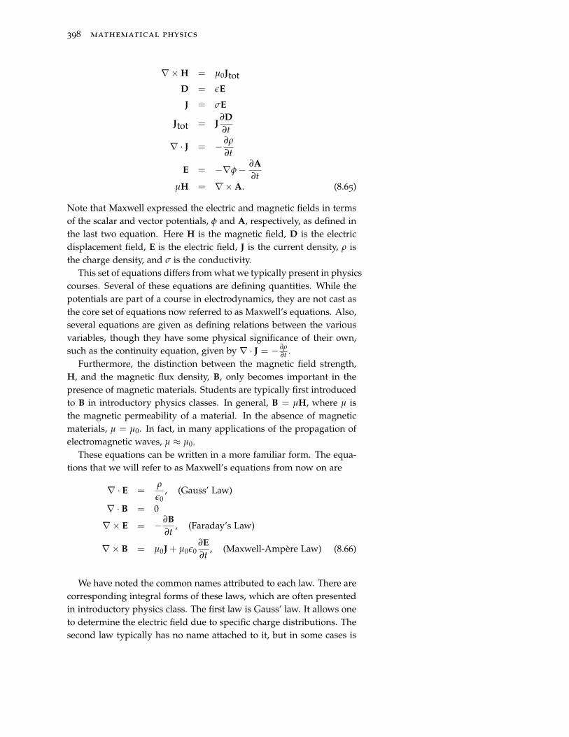
∇×H = µ0JtotD = εE
J = σE
Jtot = J∂D∂t
∇ · J = −∂ρ
∂t
E = −∇φ− ∂A∂t
µH = ∇×A. (8.65)
Note that Maxwell expressed the electric and magnetic fields in termsof the scalar and vector potentials, φ and A, respectively, as defined inthe last two equation. Here H is the magnetic field, D is the electricdisplacement field, E is the electric field, J is the current density, ρ isthe charge density, and σ is the conductivity.
This set of equations differs from what we typically present in physicscourses. Several of these equations are defining quantities. While thepotentials are part of a course in electrodynamics, they are not cast asthe core set of equations now referred to as Maxwell’s equations. Also,several equations are given as defining relations between the variousvariables, though they have some physical significance of their own,such as the continuity equation, given by ∇ · J = − ∂ρ
∂t .Furthermore, the distinction between the magnetic field strength,
H, and the magnetic flux density, B, only becomes important in thepresence of magnetic materials. Students are typically first introducedto B in introductory physics classes. In general, B = µH, where µ isthe magnetic permeability of a material. In the absence of magneticmaterials, µ = µ0. In fact, in many applications of the propagation ofelectromagnetic waves, µ ≈ µ0.
These equations can be written in a more familiar form. The equa-tions that we will refer to as Maxwell’s equations from now on are
∇ · E =ρ
ε0, (Gauss’ Law)
∇ · B = 0
∇× E = −∂B∂t
, (Faraday’s Law)
∇× B = µ0J + µ0ε0∂E∂t
, (Maxwell-Ampère Law) (8.66)
We have noted the common names attributed to each law. There arecorresponding integral forms of these laws, which are often presentedin introductory physics class. The first law is Gauss’ law. It allows oneto determine the electric field due to specific charge distributions. Thesecond law typically has no name attached to it, but in some cases is

vector analysis and em waves 399
called Gauss’ law for magnetic fields. It simply states that there areno free magnetic poles. The third law is Faraday’s law, indicating thatchanging magnetic flux induces electric potential differences. Lastly,the fourth law is a modification of Ampere’s law that states that electriccurrents produce magnetic fields.
It should be noted that the last term in the fourth equation wasintroduced by Maxwell. As we have seen, the divergence of the curl ofany vector is zero, The divergence of the curl of any vector
is zero.∇ · (∇×V) = 0.
Computing the divergence of the curl of the electric field, we find fromMaxwell’s equations that
∇ · (∇× E) = −∇ · ∂B∂t
= − ∂
∂t∇ · B = 0. (8.67)
Thus, the relation works here.However, before Maxwell, Ampère’s law in differential form would Ampère’s law in differential form.
have been written as
∇× B = µ0J.
Computing the divergence of the curl of the magnetic field, we have The introduction of the displacementcurrent makes Maxwell’s equationsmathematically consistent.∇ · (∇× B) = µ0∇ · J
= −µ0∂ρ
∂t. (8.68)
Here we made use of the continuity equation,
µ0∂ρ
∂t+ µ0∇ · J = 0.
As you can see, the vector identity, div curl = 0, does not workhere! Maxwell argued that we need to account for a changing chargedistribution. He introduced what he called the displacement current,µ0ε0
∂E∂t into the Ampère Law. Now, we have
∇ · (∇× B) = µ0∇ ·(
J + µ0ε0∂E∂t
)= −µ0
∂ρ
∂t+ µ0ε0
∂
∂t∇ · E
= −µ0∂ρ
∂t+ µ0ε0
∂
∂t
(ρ
ε0
)= 0. (8.69)
So, Maxwell’s introduction of the displacement current was not onlyphysically important, it made the equations mathematically consistent.
400 mathematical physics
8.2.2 Electromagnetic Wave Equation
We are now ready to derive the wave equation for electromagneticwaves. We will consider the case of free space in which there are nofree charges or currents and the waves propagate in a vacuum. Wethen have Maxwell’s equations in the form Maxwell’s equations in a vacuum.
∇ · E = 0,
∇ · B = 0,
∇× E = −∂B∂t
,
∇× B = µ0ε0∂E∂t
. (8.70)
We will derive the wave equation for the electric field. You shouldconfirm that a similar result can be obtained for the magnetic field.Consider the expression ∇× (∇× E). We note that the identities give
∇× (∇× E) = ∇(∇ · E)−∇2E.
However, the divergence of E is zero, so we have
∇× (∇× E) = −∇2E. (8.71)
We can also use Faraday’s Law on the right side of this equation toobtain
∇× (∇× E) = −∇×(
∂B∂t
).
Interchanging the time and space derivatives, and using the Ampere-Maxwell Law, we find
∇× (∇× E) = − ∂
∂t(∇× B)
= − ∂
∂t
(ε0µ0
∂E∂t
)= −ε0µ0
∂2E∂t2 . (8.72)
The three dimensional wave equationsfor electric and magnetic fields in a vac-uum.
Combining the two expressions for∇× (∇×E), we have the soughtresult:
ε0µ0∂2E∂t2 = ∇2E.
This is the three dimensional equation for an oscillating electricfield. A similar equation can be found for the magnetic field,
ε0µ0∂2B∂t2 = ∇2B.
Recalling that ε0 = 8.85 × 10⁻¹² C2/Nm2 and µ0 = 4π × 10−7
N/A2, one finds that c = 3× 10⁸ m/s.

vector analysis and em waves 401
One can derive more general equations. For example, we couldlook for waves in what are called linear media. In this case one hasD = εE and B = µH. Here ε is called the electric permittivity and µ isthe magnetic permeability of the material. Then, the wave speed in avacuum, c, is replaced by the wave speed in the medium, v. It is givenby
v =1√
εµ=
cn
.
Here, n is the index of refraction, n =√
εµε0µ0
. In many materials µ ≈µ0. Introducing the dielectric constant, κ = ε
ε0, one finds that n ≈
√κ.
The wave equations lead to many of the properties of the elec-tric and magnetic fields. We can also study systems in which thesewaves are confined, such as waveguides. In such cases we can imposeboundary conditions and determine what modes are allowed to prop-agate within certain structures, such as optical fibers. However, theseequation involve unknown vector fields. We have to solve for severalinter-related component functions. In the next chapter we will lookat simpler models in order to get some ideas as to how one can solvescalar wave equations in higher dimensions. However, we will first ex-plore how the differential operators introduced in this chapter appearin different coordinate systems.
8.2.3 Potential Functions and Helmholtz’s Theorem
Another application of the use of vector analysis for study-ing electromagnetism is that of potential theory. In this section we de-scribe the use of a scalar potential, φ(r, t) and a vector potential, A(r, t)to solve problems in electromagnetic theory. Helmholtz’s theorem says
Hermann Ludwig Ferdinand vonHelmholtz (1821-1894) made manycontributions to physics. There areseveral theorems named after him.
that a vector field is uniquely determined by knowing its divergenceand its curl. Combining this result with the definitions of the electricand magnetic potentials, we will show that Maxwell’s equations willthe electric and magnetic fields can be found by simply solving a setof Poisson equations, ∇2u = f , for the potential functions. A vector field is uniquely determined by
knowing its divergence and its curl.In the case of static fields, we have from Maxwell’s equationsElectric and magnetic potentials.
∇ · B = 0, ∇× E = 0.
We saw earlier in this chapter that the curl of a gradient is zero andthe divergence of a curl is zero. This suggests that E is the gradient ofa scalar function and B is the curl of a vector function:
E = −∇φ,
B = ∇×A.

402 mathematical physics
φ is called the electric potential and A is called the magnetic potential.The remaining Maxwell equations are
∇ · E =ρ
ε0, ∇× B = µ0J.
Inserting the potential functions, we have
∇2φ = − ρ
ε0, ∇× (∇×A) = µ0J.
Thus, φ satisfies a Poisson equation, which is a simple partial differ-ential equation which can be solved using separation of variables, orother techniques.
The equation satisfied by the magnetic potential looks a little morecomplicated. However, we can use the identity
∇× (∇×A) = ∇(∇ ·A)−∇2A.
If ∇ ·A = 0, then we find that
∇2A = −µ0J.
Thus, the components of the magnetic potential also satisfy Poissonequations!
It turns out that requiring ∇ · A = 0 is not as restrictive as onemight first think. Potential functions are not unique. For example,adding a constant to a potential function will still give the same fields.For example
∇(φ + c) = ∇φ = −E.
This is not too alarming because it is the field that is physical andnot the potential. In the case of the magnetic potential, adding thegradient of some field gives the same magnetic field, ∇× (A +∇ψ) =
∇×A = B. So, we can choose ψ such that the new magnetic potentialis divergenceless, ∇ · A = 0. A particular choice of the scalar andvector potentials is a called a gauge and the process is called fixing,or choosing, a gauge. The choice of ∇ · A = 0 is called the Coulombgauge. Coulomb gauge: ∇ ·A = 0.
If the fields are dynamic, i.e., functions of time, then the magneticpotential also contributes to the electric field. In this case, we have
E = −∇φ− ∂A∂t
,
B = ∇×A.
Thus, two of Maxwell’s equations are automatically satisfied,
∇ · B = 0, ∇× E = −∂B∂t
.

vector analysis and em waves 403
The other two equations become
∇ · E =ρ
ε0⇒ ∇2φ +
∂
∂t∇ ·A = − ρ
ε0,
and∇× B = µ0J + µ0ε0
∂E∂t⇒
∇(∇ ·A)−∇2A = µ0J− 1c2
∂
∂t
(∇φ +
∂A∂t
).
Rearranging, we have(∇2 − 1
c2∂2
∂t2
)A−∇
(∇ ·A +
1c2
∂φ
∂t
)= −µ0J.
If we choose the Lorentz gauge, by requiring Lorentz gauge: ∇ ·A + 1c2
∂φ∂t = 0.
∇ ·A +1c2
∂φ
∂t,
then In relativity, one defines thed’Alembertian by � ≡ 1
c2∂2
∂t2 − ∇2.Then, the equations for the potentialsbecome
�φ =ρ
ε0,
and�A = µ0J.
(∇2 − 1
c2∂2
∂t2
)φ = − ρ
ε0,(
∇2 − 1c2
∂2
∂t2
)A = −µ0J.
Thus, the potential satisfy nonhomogeneous wave equations, whichcan be solved with standard methods as one will see in a course inelectrodynamics.
The above introduction of potentials to describe the electric andmagnetic fields is a special case of Helmholtz’s Theorem for vectors.This theorem states that “any sufficiently smooth, rapidly decayingvector field in three dimensions can be resolved into the sum of an irro-tational (curl-free) vector field and a solenoidal (divergence-free) vec-tor field.”2 This is known as the Helmholtz decomposition. Namely, 2 Wikipedia entry for the Helmholtz de-
composition.given any nice vector field v, we can write it as
v = −∇φ︸ ︷︷ ︸irrotational
+ ∇×A︸ ︷︷ ︸solenoidal
.
Given∇ · v = ρ, ∇× v = F,
then one has∇2φ = ρ
and∇(∇ ·A)−∇2A = F.
Forcing ∇ ·A = 0,∇2A = −F.
Thus, one obtains Poisson equations for φ and A. This is just repeatingthe above procedure which we had seen in the special case of staticelectromagnetic fields.

404 mathematical physics
8.3 Curvilinear Coordinates
In order to study solutions of the wave equation, the heatequation, or even Schrödinger’s equation in different geometries, weneed to see how differential operators, such as the Laplacian, appearin these geometries. The most common coordinate systems arising inphysics are polar coordinates, cylindrical coordinates, and sphericalcoordinates. These reflect the common geometrical symmetries oftenencountered in physics.
In such systems it is easier to describe boundary conditions andto make use of these symmetries. For example, specifying that theelectric potential is 10.0 V on a spherical surface of radius one, wewould say φ(x, y, z) = 10 for x2 + y2 + z2 = 1. However, if we usespherical coordinates, (r, θ, φ), then we would say φ(r, θ, φ) = 10 forr = 1, or φ(1, θ, φ) = 10. This is a much simpler representation of theboundary condition.
However, this simplicity in boundary conditions leads to a morecomplicated looking partial differential equation in spherical coordi-nates. In this section we will consider general coordinate systems andhow the differential operators are written in the new coordinate sys-tems. In the next chapter we will solve some of these new problems.
We begin by introducing the general coordinate transformations be-tween Cartesian coordinates and the more general curvilinear coordi-nates. Let the Cartesian coordinates be designated by (x1, x2, x3) andthe new coordinates by (u1, u2, u3). We will assume that these are re-lated through the transformations
x1 = x1(u1, u2, u3),
x2 = x2(u1, u2, u3),
x3 = x3(u1, u2, u3). (8.73)
Thus, given the curvilinear coordinates (u1, u2, u3) for a specific pointin space, we can determine the Cartesian coordinates, (x1, x2, x3), ofthat point. We will assume that we can invert this transformation:Given the Cartesian coordinates, one can determine the correspondingcurvilinear coordinates. Need to insert figures depicting this.
In the Cartesian system we can assign an orthogonal basis, {i, j, k}.As a particle traces out a path in space, one locates its position bythe coordinates (x1, x2, x3). Picking x2 and x3 constant, the particle lieson the curve x1 = value of the x1 coordinate. This line lies in thedirection of the basis vector i. We can do the same with the other co-ordinates and essentially map out a grid in three dimensional space.All of the xi-curves intersect at each point orthogonally and the basisvectors {i, j, k} lie along the grid lines and are mutually orthogonal.
vector analysis and em waves 405
We would like to mimic this construction for general curvilinear co-ordinates. Requiring the orthogonality of the resulting basis vectorsleads to orthogonal curvilinear coordinates.
As for the Cartesian case, we consider u2 and u3 constant. Thisleads to a curve parametrized by u1 : r = x1(u1)i + x2(u1)j + x3(u1)k.We call this the u1-curve. Similarly, when u1 and u3 are constant weobtain a u2-curve and for u1 and u2 constant we obtain a u3-curve. Wewill assume that these curves intersect such that each pair of curvesintersect orthogonally. Furthermore, we will assume that the unit tan-gent vectors to these curves form a right handed system similar to the{i, j, k} systems for Cartesian coordinates. We will denote these as{u1, u2, u3}.
We can quantify all of this. Consider the position vector as a func-tion of the new coordinates,
r(u1, u2, u3) = x1(u1, u2, u3)i + x2(u1, u2, u3)j + x3(u1, u2, u3)k.
Then the infinitesimal change in position is given by
dr =∂r
∂u1du1 +
∂r∂u2
du2 +∂r
∂u3du3 =
3
∑i=1
∂r∂ui
dui.
We note that the vectors ∂r∂ui
are tangent to the ui-curves. Thus, wedefine the unit tangent vectors
ui =
∂r∂ui∣∣∣ ∂r∂ui
∣∣∣ .Solving for the tangent vector, we have
∂r∂ui
= hiui,
where The scale factors, hi ≡∣∣∣ ∂r
∂ui
∣∣∣ .
hi ≡∣∣∣∣ ∂r∂ui
∣∣∣∣are called the scale factors for the transformation.
Example 8.18. Determine the scale factors for the polar coordinate transfor-mation. Show an annotated polar plot here.
The transformation for polar coordinates is
x = r cos θ, y = r sin θ.
Here we note that x1 = x, y1 = y, u1 = r, and u2 = θ. The u1-curvesare curves with θ = const. Thus, these curves are radial lines. Similarly,the u2-curves have r = const. These curves are concentric circles about theorigin.
406 mathematical physics
The unit vectors are easily found. We will denote them by ur and uθ . Wecan determine these unit be first computing ∂r
∂ui. Let
r = x(r, θ)i + y(r, θ)j = r cos θi + r sin θj.
Then,
∂r∂r
= cos θi + sin θj
∂r∂θ
= −r sin θi + r cos θj. (8.74)
The first vector already is a unit vector. So,
ur = cos θi + sin θj.
The second vector has length r since | − r sin θi + r cos θj| = r. Dividing ∂r∂θ
by r, we haveuθ = − sin θi + cos θj.
We can see these vectors are orthogonal and form a right hand system. Thatthey form a right hand system can be seen by either drawing the vectors, orcomputing the cross product,
(cos θi + sin θj)× (− sin θi + cos θj) = k.
Since
∂r∂r
= ur,
∂r∂θ
= ruθ ,
The scale factors are hr = 1 and hθ = r.
We have determined that once we know the scale factors, we havethat
dr =3
∑i=1
hiduiui.
The infinitesimal arclength is then given by
ds2 = dr · dr =3
∑i=1
h2i du2
i
when the system is orthogonal. Also, along the ui-curves,
dr = hiduiui, (no summation).
So, we consider at a given point (u1, u2, u3) an infinitesimal paral-lelepiped of sides hidui, i = 1, 2, 3. This infinitesimal parallelepipedhas a volume of size
dV =
∣∣∣∣ ∂r∂u1· ∂r
∂u2× ∂r
∂u3
∣∣∣∣ du1du2du3.

vector analysis and em waves 407
The triple scalar product can be computed using determinants and theresulting determinant is call the Jacobian, and is given by
J =
∣∣∣∣ ∂(x1, x2, x3)
∂(u1, u2, u3)
∣∣∣∣=
∣∣∣∣ ∂r∂u1· ∂r
∂u2× ∂r
∂u3
∣∣∣∣=
∣∣∣∣∣∣∣∂x1∂u1
∂x2∂u1
∂x3∂u1
∂x1∂u2
∂x2∂u2
∂x3∂u2
∂x1∂u3
∂x2∂u3
∂x3∂u3
∣∣∣∣∣∣∣ . (8.75)
Therefore, the volume element can be written as
dV = J du1du2du3 =
∣∣∣∣ ∂(x1, x2, x3)
∂(u1, u2, u3)
∣∣∣∣ du1du2du3.
Example 8.19. Determine the volume element for cylindrical coordinates(r, θ, z), given by
x = r cos θ, (8.76)
y = r sin θ, (8.77)
z = z. (8.78)
Here, we have (u1, u2, u3) = (r, θ, z). Then, the Jacobian is given by
J =
∣∣∣∣∂(x, y, z)∂(r, θ, z)
∣∣∣∣=
∣∣∣∣∣∣∣∂x∂r
∂y∂r
∂z∂r
∂x∂θ
∂y∂θ
∂z∂θ
∂x∂z
∂y∂z
∂z∂z
∣∣∣∣∣∣∣=
∣∣∣∣∣∣∣cos θ sin θ 0−r sin θ r cos θ 0
0 0 1
∣∣∣∣∣∣∣= r (8.79)
Thus, the volume element is given as
dV = rdrdθdz.
This result should be familiar from multivariate calculus.
Next we will derive the forms of the gradient, divergence, and curlin curvilinear coordinates. The results are given here for quick refer-ence. Gradient, divergence and curl in orthog-
onal curvilinear coordinates.
408 mathematical physics
∇φ =3
∑i=1
uihi
∂φ
∂ui
=u1
h1
∂φ
∂u1+
u2
h2
∂φ
∂u2+
u3
h3
∂φ
∂u3. (8.80)
∇ · F =1
h1h2h3
(∂
∂u1(h2h3F1) +
∂
∂u2(h1h3F2) +
∂
∂u3(h1h2F3)
).
(8.81)
∇× F =1
h1h2h3
∣∣∣∣∣∣∣h1u1 h2u2 h3u3
∂∂u1
∂∂u2
∂∂u3
F1h1 F2h2 F3h3
∣∣∣∣∣∣∣ . (8.82)
∇2φ =1
h1h2h3
(∂
∂u1
(h2h3
h1
∂φ
∂u1
)+
∂
∂u2
(h1h3
h2
∂φ
∂u2
)+
∂
∂u3
(h1h2
h3
∂φ
∂u3
))(8.83)
(8.84)
We begin the derivations of these formulae by looking at the gradi-ent, ∇φ, of the scalar function φ(u1, u2, u3). We recall that the gradient Derivation of the gradient form.
operator appears in the differential change of a scalar function,
dφ = ∇φ · dr =3
∑i=1
∂φ
∂uidui.
Since
dr =3
∑i=1
hiduiui,
we also have that
dφ = ∇φ · dr =3
∑i=1
(∇φ)i hidui.
Comparing these two expressions for dφ, we determine that the com-ponents of the del operator can be written as
(∇φ)i =1hi
∂φ
∂ui
and thus the gradient is given by
∇φ =u1
h1
∂φ
∂u1+
u2
h2
∂φ
∂u2+
u3
h3
∂φ
∂u3.
Next we compute the divergence, Derivation of the divergence form.
∇ · F =3
∑i=1∇ · (Fiui) .
We can do this by computing the individual terms in the sum. We willcompute ∇ · (F1u1) .
vector analysis and em waves 409
We first note that the gradients of the coordinate functions are found
as ∇ui =uihi
. (This results from a direct application of the gradient
operator form just derived.) Then
∇u2 ×∇u3 =u2 × u3
h2h3=
u1
h2h3.
This gives
∇ · (F1u1) = ∇ · (F1h2h3∇u2 ×∇u3)
= ∇ (F1h2h3) · ∇u2 ×∇u3 + F1h2h2∇ · (∇u2 ×∇u3).
(8.85)
Here we used the vector identity
∇ · ( f A) = f∇ ·A + A · ∇ f
The second term can be handled using the identity
∇ · (A× B) = B · (∇×A)−A · (∇× B),
where A and B are gradients. However, each term the curl of a gradi-ent, which are identically zero! Or, you could just use the third identityin the previous list of second derivative identities,
∇ · (∇ f ×∇g) = 0.
Using the expression ∇u2 ×∇u3 = u1h2h3
and the expression for thegradient operator in curvilinear coordinates, we have
∇ · (F1u1) = ∇ (F1h2h3) ·u1
h2h3=
1h1h2h3
∂
∂u1(F1h2h3) .
Similar computations can be done for the remaining components,leading to the sought expression for the divergence in curvilinear co-ordinates:
∇ · F =1
h1h2h3
(∂
∂u1(h2h3F1) +
∂
∂u2(h1h3F2) +
∂
∂u2(h1h2F3)
).
We now turn to the curl operator. In this case, we need to simplify Derivation of the curl form.
∇× F =3
∑i=1∇× (Fiui) .
Using the identity
∇× ( f A) = f∇×A−A×∇ f ,
we have
∇× (F1u1) = ∇× (F1h1∇u1)
= ∇ (F1h1)×∇u1 + F1h1∇×∇u1. (8.86)

410 mathematical physics
Again, the curl of the gradient vanishes, leaving
∇× (F1u1) = ∇ (F1h1)×∇u1.
Since ∇u1 = u1h1
, we have
∇× (F1u1) = ∇ (F1h1)×u1
h1
=
(3
∑i=1
uihi
∂ (F1h1)
∂ui
)× u1
h1
=u2
h3h1
∂ (F1h1)
∂u3− u3
h1h2
∂ (F1h1)
∂u2. (8.87)
The other terms can be handled in a similar manner. The overallresult is that
∇× F =u1
h2h3
(∂ (h3F3)
∂u2− ∂ (h2F2)
∂u3
)+
u2
h1h3
(∂ (h1F1)
∂u3− ∂ (h3F3)
∂u1
)+
u3
h1h2
(∂ (h2F2)
∂u1− ∂ (h1F1)
∂u2
)(8.88)
This can be written more compactly as
∇× F =1
h1h2h3
∣∣∣∣∣∣∣h1u1 h2u2 h3u3
∂∂u1
∂∂u2
∂∂u3
F1h1 F2h2 F3h3
∣∣∣∣∣∣∣ (8.89)
Finally, we turn to the Laplacian. In the next chapter we will solvehigher dimensional problems in various geometric settings such as thewave equation, the heat equation, and Laplace’s equation. These allinvolve knowing how to write the Laplacian in different coordinatesystems. Since ∇2φ = ∇ ·∇φ, we need only combine the above resultsfor the gradient and the divergence in curvilinear coordinates. This isstraight forward and gives
∇2φ =1
h1h2h3
(∂
∂u1
(h2h3
h1
∂φ
∂u1
)+
∂
∂u2
(h1h3
h2
∂φ
∂u2
)+
∂
∂u3
(h1h2
h3
∂φ
∂u3
)). (8.90)
The results of rewriting the standard differential operators in cylin-drical and spherical coordinates are shown in Problems 28 and 29. Inparticular, the Laplacians are given as
vector analysis and em waves 411
Cylindrical Coordinates:
∇2 f =1r
∂
∂r
(r
∂ f∂r
)+
1r2
∂2 f∂θ2 +
∂2 f∂z2 . (8.91)
Spherical Coordinates:
∇2 f =1ρ2
∂
∂ρ
(ρ2 ∂ f
∂ρ
)+
1ρ2 sin θ
∂
∂θ
(sin θ
∂ f∂θ
)+
1ρ2 sin2 θ
∂2 f∂φ2 .
(8.92)
These forms will be used in the next chapter for the solution ofLaplace’s equation, the heat equation, and the wave equation in thesecoordinate systems.
Problems
1. Compute u× v using the permutation symbol. Verify your answerby computing these products using traditional methods.
a. u = 2i− 3k, v = 3i− 2j.
b. u = i + j + k, v = i− k.
c. u = 5i + 2j− 3k, v = i− 4j + 2k.
2. Compute the following determinants using the permutation sym-bol. Verify your answer.
a.
∣∣∣∣∣∣∣3 2 01 4 −2−1 4 3
∣∣∣∣∣∣∣b.
∣∣∣∣∣∣∣1 2 24 −6 32 3 1
∣∣∣∣∣∣∣3. For the given expressions, write out all values for i, j = 1, 2, 3.
a. εi2j.
b. εi13.
c. εij1εi32.
4. Show that
a. δii = 3.
b. δijεijk = 0
c. εimnεjmn = 2δij.
d. εijkεijk = 6.
412 mathematical physics
5. Show that the vector (a×b)× (c×d) lies on the line of intersectionof the two planes: (1) the plane containing a and b and (2) the planecontaining c and d.
6. Prove the following vector identities:
a. (a× b) · (c× d) = (a · c)(b · d)− (a · d)(b · c).b. (a× b)× (c× d) = (a · b× d)c− (a · b× c)d.
7. Use problem 6a to prove that |a× b| = ab sin θ.
8. A particle moves on a straight line, r = tu, from the center of adisk. If the disk is rotating with angular velocity ω, then u rotates. Letu = (cos ωt)i + (sin ωt)j.
a. Determine the velocity, v.
b. Determine the acceleration, a.
c. Describe the resulting acceleration terms identifying the cen-tripetal acceleration and Coriolis acceleration.
9. Compute the gradient of the following:
a. f (x, y) = x2 − y2.
b. f (x, y, z) = yz + xy + xz.
c. f (x, y) = tan−1 ( yx)
.
d. f (x, y, z) =
10. Find the directional derivative of the given function at the indi-cated point in the given direction.
a. f (x, y) = x2 − y2, (3, 2), u = i + j.
b. f (x, y) = yx , (2, 1), u = 3i + 4j.
c. f (x, y, z) = x2 + y2 + z2, (1, 0, 2), u = 2i− j.
11. Zaphod Beeblebrox was in trouble after the infinite improbabilitydrive caused the Heart of Gold, the spaceship Zaphod had stolen whenhe was President of the Galaxy, to appear between a small insignificantplanet and its hot sun. The temperature of the ship’s hull is given byT(x, y, z) = e−k(x2+y2+z2) Nivleks. He is currently at (1, 1, 1), in units ofglobs, and k = 2 globs−2. (Check the Hitchhikers Guide for the currentconversion of globs to kilometers and Nivleks to Kelvins.)
a. In what direction should he proceed so as to decrease thetemperature the quickest?
b. If the Heart of Gold travels at e6 globs per second, then howfast will the temperature decrease in the direction of fastestdecline?
vector analysis and em waves 413
12. For the given vector field, find the divergence and curl of the field.
a. F = xi + yj.
b. F = yr i− x
r j, for r =√
x2 + y2.
c. F = x2yi + zj + xyzk.
13. Write the following using εijk notation and simplify if possible.
a. C× (A× (A× C)).
b. ∇ · (∇×A).
c. ∇×∇φ.
14. Prove the identities:
a. ∇ · (∇×A) = 0.
b. ∇ · ( f∇g− g∇ f ) = f∇2g− g∇2 f .
c. ∇rn = nrn−2r, n ≥ 2.
15. For r = xi + yj + zk and r = |r|, simplify the following.
a. ∇× (k× r).
b. ∇ ·( r
r)
.
c. ∇×( r
r)
.
d. ∇ ·(
rr3
).
16. Newton’s Law of Gravitation gives the gravitational force betweentwo masses as
F = −GmMr3 r.
a. Prove that F is irrotational.
b. Find a scalar potential for F.
17. Consider an electric dipole moment p at the origin. It producesan electric potential of φ = p·r
4πε0r3 outside the dipole. Noting thatE = −∇φ, find the electric field at r.
18. In fluid dynamics the Euler equations govern inviscid fluid flowand provide quantitative statements on the conservation of mass, mo-mentum and energy. The continuity equation is given by
∂ρ
∂t+∇ · (ρv) = 0,
where ρ(x, y, z, t) is the mass density and v(x, y, z, t) is the fluid veloc-ity. The momentum equations are given by
∂ρv∂t
+ v · ∇(ρv) = f−∇p.
Here p(x, y, z, t) is the pressure and F is the external force per volume.
414 mathematical physics
a. Show that the continuity equation can be rewritten as
∂ρ
∂t+ ρ∇ · (v) + v · ∇ρ = 0.
b. Prove the identity 12∇v2 = v · ∇v for irrotational v.
c. Assume that
• the external forces are conservative (F = −∇φ),
• the velocity field is irrotational (∇× v = 0).
• the fluid is incompressible (ρ =const), and
• the flow is steady, ∂v∂t = 0.
Under these assumptions, prove Bernoulli’s Principle:
12
v2 + φ +pρ= const.
19. Find the lengths of the following curves:
a. y(x) = x for x ∈ [0, 2].
b. (x, y, z) = (t, ln t, 2√
2t) for 1 ≤ t ≤ 2.
c. y(x) = 2 cosh 3x, x ∈ [−2, 2]. (Recall the hanging chain ex-ample from classical dynamics.)
20. Consider the integral∫
C y2 dx − 2x2 dy. Evaluate this integral forthe following curves:
a. C is a straight line from (0,2) to (1,1).
b. C is the parabolic curve y = x2 from (0,0) to (2,4).
c. C is the circular path from (1,0) to (0,1) in a clockwise direc-tion.
21. Evaluate∫
C(x2 − 2xy + y2) ds for the curve x(t) = 2 cos t, y(t) =2 sin t, 0 ≤ t ≤ π.
22. Prove that the magnetic flux density, B, satisfies the wave equation.
23. Prove the identity∫C
φ∇φ · n ds =∫
D(φ∇2φ +∇ · ∇φ) dA.
24. Compute the work done by the force F = (x2− y2)i+ 2xyj in mov-ing a particle counterclockwise around the boundary of the rectangleR = [0, 3]× [0, 5].
25. Compute the following integrals:
a.∫
C(x2 + y) dx + (3x + y3) dy for C the ellipse x2 + 4y2 = 4.
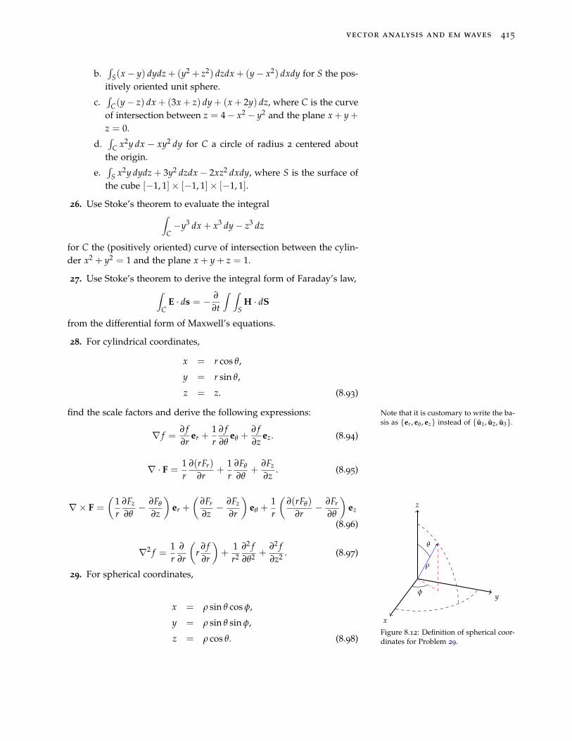
vector analysis and em waves 415
b.∫
S(x− y) dydz + (y2 + z2) dzdx + (y− x2) dxdy for S the pos-itively oriented unit sphere.
c.∫
C(y− z) dx + (3x + z) dy + (x + 2y) dz, where C is the curveof intersection between z = 4− x2− y2 and the plane x + y +z = 0.
d.∫
C x2y dx − xy2 dy for C a circle of radius 2 centered aboutthe origin.
e.∫
S x2y dydz + 3y2 dzdx− 2xz2 dxdy, where S is the surface ofthe cube [−1, 1]× [−1, 1]× [−1, 1].
26. Use Stoke’s theorem to evaluate the integral∫C−y3 dx + x3 dy− z3 dz
for C the (positively oriented) curve of intersection between the cylin-der x2 + y2 = 1 and the plane x + y + z = 1.
27. Use Stoke’s theorem to derive the integral form of Faraday’s law,∫C
E · ds = − ∂
∂t
∫ ∫S
H · dS
from the differential form of Maxwell’s equations.
28. For cylindrical coordinates,
x = r cos θ,
y = r sin θ,
z = z. (8.93)
find the scale factors and derive the following expressions: Note that it is customary to write the ba-sis as {er , eθ , ez} instead of {u1, u2, u3}.
∇ f =∂ f∂r
er +1r
∂ f∂θ
eθ +∂ f∂z
ez. (8.94)
∇ · F =1r
∂(rFr)
∂r+
1r
∂Fθ
∂θ+
∂Fz
∂z. (8.95)
∇× F =
(1r
∂Fz
∂θ− ∂Fθ
∂z
)er +
(∂Fr
∂z− ∂Fz
∂r
)eθ +
1r
(∂(rFθ)
∂r− ∂Fr
∂θ
)ez
(8.96)
∇2 f =1r
∂
∂r
(r
∂ f∂r
)+
1r2
∂2 f∂θ2 +
∂2 f∂z2 . (8.97)
29. For spherical coordinates,
x
y
z
ρ
φ
θ
Figure 8.12: Definition of spherical coor-dinates for Problem 29.
x = ρ sin θ cos φ,
y = ρ sin θ sin φ,
z = ρ cos θ. (8.98)

416 mathematical physics
find the scale factors and derive the following expressions:
∇ f =∂ f∂ρ
eρ +1ρ
∂ f∂θ
eθ +1
ρ sin θ
∂ f∂φ
eφ. (8.99)
∇ · F =1ρ2
∂(ρ2Fρ)
∂ρ+
1ρ sin θ
∂(sin θFθ)
∂θ+
1ρ sin θ
∂Fφ
∂φ. (8.100)
∇× F =1
ρ sin θ
(∂(sin θFφ)
∂θ− ∂Fθ
∂φ
)eρ +
1ρ
(1
sin θ
∂Fρ
∂φ−
∂(ρFφ)
∂ρ
)eθ
+1ρ
(∂(ρFθ)
∂ρ−
∂Fρ
∂θ
)eφ (8.101)
∇2 f =1ρ2
∂
∂ρ
(ρ2 ∂ f
∂ρ
)+
1ρ2 sin θ
∂
∂θ
(sin θ
∂ f∂θ
)+
1ρ2 sin2 θ
∂2 f∂φ2 .
(8.102)