27

“VARIATION-TALK”: ARTICULATING MEANING IN STATISTICS7

KATIE MAKARUniversity of Queensland, Australia

k.makar@uq.edu.au

JERE CONFREYWashington University in St. Louis, U.S.A.

jconfrey@wustl.edu

SUMMARY

Little is known about the way that teachers articulate notions of variation in their own words. Thestudy reported here was conducted with 17 prospective secondary math and science teachersenrolled in a preservice teacher education course which engaged them in statistical inquiry oftesting data. This qualitative study examines how these preservice teachers articulated notions ofvariation as they compared two distributions. Although the teachers made use of standardstatistical language, they also expressed rich views of variation through nonstandardterminology. This paper details the statistical language used by the prospective teachers,categorizing both standard and nonstandard expressions. Their nonstandard language revealedstrong relationships between expressions of variation and expressions of distribution.Implications and the benefits of nonstandard language in statistics are outlined.

Keywords: Statistical reasoning; Statistics education; Reasoning about variation and distribution;Mathematics education; Teacher education; Nonstandard language

Do not let calculations override common sense.

Moore & McCabe (1993, p. 121)

1. INTRODUCTION

Recently, researchers in statistics education have been calling for greater emphasis in schools ondeveloping students’ conceptions of variation (Moore, 1990; Shaughnessy, Watson, Moritz, &Reading, 1999; Pfannkuch & Begg, 2004). In addition, they argue that too much instruction instatistics has focused on performing statistical operations rather than developing students’ thinkingabout what makes sense. One approach to sense-making is through encouraging learners to expresstheir ideas in their own words (Noss & Hoyles, 1996). Russell and Mokros (1990) documentedteachers’ statistical thinking by attending to their ways of describing data using nonstandard statisticallanguage. Other research has also revealed that learners often articulate concepts of variation usingnonstandard language (e.g., Bakker, 2004; Reading, 2004); however these studies have notsystematically looked at ways that learners express notions of variation. Even less is known abouthow teachers express concepts of variation.

In other qualitative studies, we examined preservice secondary mathematics and science teachers’experiences making sense of data as they conducted technology-based investigations (Confrey,Makar, & Kazak, 2004; Makar, 2004; Makar & Confrey, submitted). This paper reports on anexploratory study of preservice teachers’ use of standard and nonstandard statistical language whendiscussing notions of variation. Below we first review the background for the present study, including

Statistics Education Research Journal, 4(1), 27-54, http://www.stat.auckland.ac.nz/serj

© International Association for Statistical Education (IASE/ISI), May, 2005

28

the conceptualization of variation, prior research on teachers’ and students’ knowledge of variation,and research needs regarding meaning construction and language use in statistics education.

2. REASONING ABOUT VARIATION

Although variation is a central component of understanding statistics, little is known about howchildren (and even less about how teachers) reason with, conceptualize, learn about, and expressnotions of variation. This section begins with a conceptual analysis of variation, then looks at recentresearch on developing teachers’ conceptions of variation, and finally turns to recent work on middleschool students’ reasoning in this area.

2.1. VARIATION AS A CONCEPTUAL ENTITY

Most uses of the term “variation” in research studies are taken to have a self-evident, commonsense meaning, and leave it undefined. Variation is closely linked to the concepts of variable anduncertainty. It is often regarded as a measurement of the amount that data deviate from a measure ofcenter, such as with the interquartile range or standard deviation. Variation encompasses more than ameasure, although measuring variation is an important component in data analysis. In consideringvariation, one must consider not just what it is (its definition or formula), or how to use it as a tool(related procedures), but also why it is useful within a context (purpose).

In simple terms, variation is the quality of an entity (a variable) to vary, including variation due touncertainty. “Uncertainty and variability are closely related: because there is variability, we live inuncertainty, and because not everything is determined or certain, there is variability” (Bakker, 2004,p. 14). While no one expects all five year-old children to be the same height, there is often difficultyunderstanding the extent to which children’s height vary, and that the variability of their heights is amixture of explained factors (e.g., the parents’ heights, nutrition) and chance or unexplained factors.

In this paper, we will not distinguish between reasoning about variability and reasoning aboutvariation, although Reading and Shaughnessy’s (2004, p. 202) definition of variation distinguishes itfrom variability:

The term variability will be taken to mean the [varying] characteristic of the entity that isobservable, and the term variation to mean the describing or measuring of that characteristic.Consequently, the following discourse, relating to “reasoning about variation,” will deal withthe cognitive processes involved in describing the observed phenomenon in situations thatexhibit variability, or the propensity for change.

We would argue that developing the concept of variation, beyond just an acknowledgement of itsexistence, requires some understanding of distribution. In examining a variable in a data set, one isoften interested in uncovering patterns in the variability of the data (Bakker, 2004), for example byrepresenting the ordered values of the variable in a graph. The distribution, then, becomes a visualrepresentation of the data’s variation and understanding learners’ concept of variation becomesclosely linked to understanding their concept of distribution. A key goal in developing students’reasoning about distributions is assisting them in seeing a distribution as an aggregate with its owncharacteristics (such as its shape or its mean) rather than thinking of a distribution as a collection ofindividual points (Hancock, Kaput, & Goldsmith, 1992; Konold & Higgins, 2002; Marshall, Makar,& Kazak, 2002; Bakker, 2004).

In thinking about what the notion of distribution entails, one might think of the associatedmeasures, properties, or characteristics of a distribution—for example, its mean, shape, outliers, orstandard deviation. These entities in isolation, however, do not capture the desired concept and canaggravate the focus on individual points. In addition, they lack the idea that we want to capture adistribution of something. Pfannkuch, Budgett, Parsonage, and Horring (2004) cautioned that studentsoften focus on characteristics of a distribution, but forget to focus on the meaning of the distribution

29

within the context of the problem. In comparing distributions, for example, they suggested thatstudents should first look at the distributions and compare centers, spread, and anything noteworthy,but then should be asked to draw an evidence-based conclusion, using probabilistic rather thandeterministic language, based on their observations.

2.2. TEACHERS’ REASONING ABOUT VARIATION

Teachers’ mind-set and conceptions about data have been of great concern in the researchcommunity for over a decade (Hawkins, 1990; Shaughnessy, 1992). Despite this, Shaughnessy (2001)reports, “[I am] not aware of any research studies that have dealt specifically with teachers’conceptions of variability, although in our work teaching statistics courses for middle school andsecondary school mathematics teachers we have evidence that many teachers have a knowledge gapabout the role and importance of variability.”

Three very recent research projects have focused specifically on teachers’ notions of variation anddistribution. Hammerman and Rubin (2004) report on a study of a two-year professional developmentproject that gave secondary teachers an opportunity to analyze data with a new data visualization tool.The software Tinkerplots™ (Konold & Miller, 2004) allows learners to create their own datarepresentations through sorting, ordering, and stacking data. They found that teachers did not chooseto use measures of center in comparing distributions even though those measures were readilyavailable in the software, but rather chose to compare groups by comparing slices and subsets ofdistributions to support compelling arguments with data. In addition, Hammerman and Rubin notedthat teachers were dissatisfied with representations such as histograms and box plots that would hidethe detail of the underlying distribution. From their study, we can begin to see the potential that newvisualization tools have for helping teachers to construct their own meaning of statistical concepts.

In another study, Canada (2004) created a framework to investigate prospective elementaryteachers’ expectation, display, and interpretation of variation within three statistical contexts: repeatedsampling, data distributions, and probability outcomes. His study took place in a preservicemathematics course developed to build the teachers’ content knowledge of probability and statisticsthrough activities that emphasized hands-on experiments involving chance and computer-generateddata simulations. Canada’s study found that initially, although the prospective teachers had a goodsense of center, they found it difficult to predict realistic spreads in distributions from collected dataor produced from random sampling and probability experiments. Their predictions for underlyingdistributions included expectations of way too little variation, overly extreme variation, orunrealistically symmetrical distributions. In addition, many of the teachers took an initial stance that‘anything goes’ in random experiments and felt that they could therefore make no judgment about thedistribution of outcomes. After the course, the teachers demonstrated stronger intuitions aboutvariation - their predictions were much more realistic and their expectation of variation morebalanced. In addition, the teachers’ descriptions of distributions were more rich and robust in theirrecognition of variation and distribution as an important concept, for example by referencing how thedistributions were clustered, spread, concentrated, or distributed. Canada’s study hints at a potentiallink between the elements that teachers focus on when describing distributions and their intuitionabout variation and uncertainty in data.

In previous research on statistical inquiry with practicing middle school teachers, we found thatteachers, like their students, often begin examining data distributions by focusing on individual points(Confrey & Makar, 2002). Yet in a meaningful context (e.g., student test scores), the teachers in ourstudy constructed a need for examining variation in a distribution by initiating a discussion of how thedistribution of students’ abilities affected their choice of instructional strategies. We noticed,however, that when the teachers did not adequately construct more complex concepts, like samplingdistributions, they would tend to use statistical tools mechanically, without carefully examining theirrelationship to the data (Makar & Confrey, 2004).

In summary, although much concern has been expressed about the over-emphasis on proceduresin teaching statistics, the studies described above highlight some important ways to improve whatShaughnessy (1992) calls teachers’ lack of intuition about stochastics. The main ideas these studies

30

bring out is that teachers themselves need to learn statistical concepts in an environment much like theone recommended for students – one that is active, technology-rich, involving authentic data, andoffering plenty of opportunities to build their conceptions through experiences with data. Particularsabout how teachers build these conceptions still needs further research.

2.3. STUDENTS’ REASONING ABOUT VARIATION

It is useful to briefly review research on students’ development of concepts of variation, as it mayprovide insight into potential ways to build teachers’ conceptions of variation. First, teachersfrequently possess similar reasoning to their students (Hammerman & Rubin, 2004; McClain, 2002).Second, understanding students’ conceptions of variation can help teachers to plan instruction.Finally, the research in this area has uncovered new insights into students’ intuitions about variationwithout formal procedures and terminology. These insights may provide ideas for new methods ofprofessional development for teachers.

A common thread in the research on teaching concepts of variation and distribution is arecommendation to focus not only on the characteristics of distributions, but on their purpose. A well-documented approach to this is through comparing groups (see for example, Cobb, 1999; Watson &Moritz, 1999; Biehler, 1997; Makar & Confrey, 2004; Hammerman & Rubin, 2004). Pfannkuch et al.(2004) found that the descriptions of distributions given by secondary students sometimes includedcharacteristics of the distribution that were disconnected from the context or meaning of the problem.For example, when taking note of the variability of the data, half of the students compared the ranges,which was not relevant to their question, and most of the students focused on comparing measures ofcenter or extremes. Pfannkuch and her colleagues hypothesized that the instruction the studentsreceived focused not on drawing meaningful conclusions, but rather on comparing features of the boxplot. They recommended that instruction concentrate not on how to compare centers, but why oneshould do so. Reading and Shaughnessy (2004) also found that tasks which asked students not just fordescriptive information but also for explanations offered greater possibilities for insight into students'reasoning about variation.

In developing students’ conception of statistics, Konold and Pollatsek (2002) argue that “thecentral idea should be that of searching for a signal and that the idea of distribution comes into betterfocus when it is viewed as the ‘distribution around’ a signal” (p. 262). Bakker and Gravemeijer (2004)on the other hand hold that “reasoning with shapes forms the basis for reasoning about distributions”(p. 149). By developing a lens of seeing the distribution as an entity, one can then look at statisticalmeasures as characteristics of the distribution rather than as calculations from individual points(Bakker, 2004).

Bakker (2004; Bakker & Gravemeijer, 2004) also found that with Cobb’s Minitool software andan innovative learning trajectory he was able to encourage his middle school students to think aboutvariation and towards a distribution-view of data. Initial discussions with students focused on themiddle “bump” of the distribution, but later the “bump” came to represent the whole distribution.Konold and his colleagues (2002), who studied middle school students, emphasized that in problemsolving with data, the middle bump was a frequently identified portion of a mound-shapeddistribution, and termed this central bump a modal clump. Bakker (2004) also found that rather thanjust focusing on the central region of a distribution, students also tend to divide distributions into threecategories: low, middle, and high. Hammerman and Rubin (2004) saw the teachers in their study takea similar tactic in comparing distributions. These findings may indicate that dividing distributions intothree pieces may be a more natural way for students to examine a distribution than by dividing it intofour sections, as in the box plot.

The studies reported above suggest that if learners are provided with relevant contexts, concreteexperiences, complex tasks, adequate time and support, and appropriate tools to build statisticalconcepts, then their understanding appears to be much more robust. One notable common feature ofthese studies is that they developed learners’ notions of variation through constructing a purpose forvariation, often building on the learners’ own language for describing and interpreting what they wereseeing.

31

3. CONCEPT DEVELOPMENT

Below we briefly discuss some aspects of how learners construct meaning of data as well asissues surrounding the use of learners’ everyday or nontechnical terminology. These issues affectedthe design of the present study and the lens we used to interpret prospective teachers’ articulation ofvariation. The need to refer both to standard statistical terminology and to nonstandard ornontechnical statistical terminology arises because one cannot assume that if a respondent can repeatthe definition of a concept, she has necessarily assimilated this concept. For example, although astudent may be taught the concept and formula for standard variation and can even use this term aspart of class discourse, this does not imply that they are “seeing” variation in what is being measured.

3.1. CONSTRUCTING MEANING

Because students are frequently taught definitions and procedures without first developing theirown intuition and meaning about the concepts underlying them, premature instruction of formalterminology and rules can inhibit students’ own sense-making (Flyvbjerg, 2001; Schoenfeld, 1991;Boaler, 1997). Formal mathematical procedures, terminology, and symbolism are critical fordeveloping advanced levels of mathematical understanding in that they can provide efficient paths toproblem-solving, focus attention on particular aspects of a problem, and open new levels ofunderstanding of the concepts represented by the terms or symbols. However, the emphasis must beon building meaning, not simply assuming that standard procedures or terms can themselves carry themeanings of underlying concepts.

Shaughnessy (1992) notes that students’ and teachers’ lack of intuition about stochastics is acritical barrier to improved teaching and learning in statistics. Fischbein’s (1987) description ofintuition matches well with the kind of thinking that we believed should be developed in teachers.

Intuitions are always the product of personal experience, of the personal involvement of theindividual in a certain practical or theoretical activity. Only when striving to cope activelywith certain situations does one need such global, anticipatory, apparently self-consistentrepresentations. The development of … intuitions implies, then, didactical situations in whichthe student is asked to evaluate, to conjecture, to predict, to devise, and check solutions. Inorder to develop new, correct probabilistic intuitions, for instance, it is necessary to createsituations in which the student has to cope, practically, with uncertain events (p. 213, italics inoriginal).

For building intuition, Fischbein further argues that the role of visualization “is so important that veryoften intuitive knowledge is identified with visual representations” (p. 103). Insight can also be gainedinto learners’ sense-making by focusing on how they use their own words to explain relationships,constructs, and processes (Noss & Hoyles, 1996). One might infer from these last three quotes thatintuition in statistics is built through the development of visualization, articulation, and representationof data distributions within personally compelling contexts. Intuition about variation, then, may befostered through a lens of “seeing variation” (Watkins, Scheaffer, & Cobb, 2003, p. 10), or Moore’s(1990) acknowledgement of the omnipresence of variation. These insights may be gained throughattending to students’ own words for describing what they are seeing. These words are often lesstechnical and contain elements of nonstandard language.

3.2. NONSTANDARD LANGUAGE USE

Noss and Hoyles (1996) state that focusing on mathematical meaning moves us to consider howlearners express mathematics rather than how they learn it. The difference is in the locus of theconcept. If we focus on how students learn statistics, it implies that statistical concepts areontologically fixed and that the goal of learning is to impart a priori knowledge from teacher to

32

student. However, by turning that around to foster learners’ dynamic conceptions of statisticalconcepts, we acknowledge that these concepts are not passively received, but rather are actively andsocially constructed by the individual.

Developing understanding oftentimes requires the use of nonstandard terminology. Unfortunately,when students do use their own language to make meaning, teachers often do not recognizenonstandard ways of talking (Lemke, 1990). Biehler (1997) attributes some of the difficulty incommunicating and understanding relationships in data to the lack of formal language we have indescribing distributions beyond the level of statistical summaries:

The description and interpretation of statistical graphs and other results is also a difficultproblem for interviewers and teachers. We must be more careful in developing a language forthis purpose and becoming aware of the difficulties inherent in relating different systems ofrepresentation. Often, diagrams involve expressing relations of relations between numbers. Anadequate verbalization is difficult to achieve and the precise wording of it is often critical.There are profound problems to overcome in interpreting and verbally describing statisticalgraphs and tables that are related to the limited expressability of complex quantitative relationsby means of common language (p. 176).

Biehler’s work implies that the current focus on statistical summaries in describing distributions isinadequate and that research needs to be improved in the area of developing statistical language forinterpreting more robust relationships in data.

4. DESIGN AND METHODOLOGY

4.1. APPROACH

This exploratory study was designed to gain insight into the ways that prospective secondarymathematics and science teachers express or discuss notions of variation when engaged in apurposeful statistical task. Based on the literature reviewed, it was anticipated that respondents willuse standard or conventional descriptions and terms, as well as nonstandard descriptions and informallanguage, and the goal of the study was to document the different types of language used.Respondents were interviewed twice using an identical task, in the first and last week of a fifteen-week preservice course on assessment, which included an embedded component of exploratory dataanalysis. The task given during the interview asked teachers to compare two distributions of datarelevant to the context of teaching, in terms of the relative improvement in test scores of two groupsof students.

Although interviews were conducted at the beginning and end of the course, the purpose of thestudy was not to evaluate the effectiveness of the course or to compare performance before and afterinstruction. Some comparisons will be made of language use before and after the course, but given thesmall number of respondents, these comparisons should be interpreted with caution. The primaryinterest was in categorizing and describing the language respondents use to describe variation in thedata. Any change that may have occurred in respondents’ language use simply enriched and extendedthe range of responses available for analysis.

4.2. SUBJECTS

The respondents for the study were secondary mathematics and science preservice teachers at alarge university in the southern United States enrolled in an innovative one-semester undergraduatecourse on assessment designed and taught by the authors (Confrey et al., 2004). Twenty-two studentsbegan the course, but four withdrew from the course before the end of the semester. In addition, somedata from one subject was lost due to technical malfunction, leaving seventeen subjects with acomplete set of data. The seventeen subjects ranged in age from 19 to 42, with ten students of

33

traditional college age (19-22), five aged 23-29, and two students over 30 years of age. Of these, threewere male and fourteen female, nine were mathematics majors and eight were science majors(predominantly biology). About 60% of the class was Anglo, with the remaining students being ofHispanic and African-American ancestry. The students had varying backgrounds in statistics: eighthad not previously studied statistics, while five had previously taken a traditional university-basedstatistics course either in the mathematics department or in a social science department. Theremaining four had not taken a formal course, but had previous experience in statistics as a topic inone of their mathematics or science courses.

4.3. SETTING

The study took place at the beginning and end of a one-semester course that integrated ideas ofassessment, data analysis, equity, and inquiry—themes identified as critical but missing frompreservice education (National Research Council, 1999; 2000; 2001). The purpose of the course wasto give the preservice teachers some background in classroom and high-stakes assessment, developtheir statistical reasoning, gain experience using technological tools to interpret student assessmentresults, and to introduce them to issues of equity through examining data. In the final month of thecourse, the prospective teachers conducted their own data-based inquiry into an issue of equity inassessment.

The prospective teachers were guided through several investigations that built an atmosphere ofinterpretation of data rather than the development of formal theoretical foundations. The inclusion ofthe dynamic statistical software Fathom™ (Finzer, 2001) was critical as a learning tool rather than atraditional statistical package aimed at statisticians and statistics students. The statistical content of thecourse was comprised of an overview of data graphing (histograms, box plots, dot plots), descriptivestatistics (mean, median, standard deviation, interquartile range, distribution shapes), linear regression(association, correlation, least-squares, residuals), and a brief introduction to sampling distributionsand inference (through building of simulations). The statistical content was developed as a set of toolsto gain insight into data rather than as isolated topics.

4.4. INTERVIEW TASK AND PROCEDURE

Respondents were interviewed by the first author during the first and last week of the course,using the same task in both interviews. Most interviews lasted between ten and twenty minutes. Thetask was set in the context of an urban middle school trying to determine the effectiveness of asemester-long mathematics remediation program (called ‘Enrichment’) for eighth-grade (13-14 yearsold) students considered in need of extra help preparing for the state exam given each spring. Todecide if the Enrichment program was working, the school compared student scores from theirseventh grade state exam score in mathematics to their scores on a practice test given near the end ofeighth grade. Respondents were shown a pair of dot plots (Figure 1) of authentic data taken fromstudents in an Enrichment class (upper distribution) and a regular eighth grade class (lowerdistribution). Respondents were asked initially to compare the relative improvement of students in thetwo groups, and then were probed if their responses needed clarification. It is important to note thatthe data in Figure 1 represent the change (difference) in scores between the two assessments, i.e.numbers on the x-axis are positive when scores improved, and negative when scores declined. (Datapoints in red (shaded dots) highlighted those students classified as economically disadvantaged; thiswas used for another question in the interview related to equity but not pertinent for this study.)

34

Figure 1. Graph shown to subjects during the interview task.

The preservice teachers were walked through particular elements of the graphs both in the pre-interview (January) and post-interview (May). It was explained that the data on the horizontal axisrepresented the improvement of each student from the seventh grade state exam to their eighth gradepractice test. The mean improvement of each group, marked by a vertical line segment in eachdistribution, was pointed out. The overall mean (displayed as -5.26271 at the bottom of the graph)was interpreted to respondents as the average improvement of the entire eighth grade (that is, bothgroups combined) and it was also noted that the overall mean improvement lay in the negative region,meaning that generally the students had performed less well on their eighth grade practice test thanthey did on the seventh grade state exam.

In our choice of task we considered it important to make the context and task as authentic aspossible in order to examine the prospective teachers’ responses in a situation close to what theywould encounter in their professional life. Therefore, rather than use hypothetical data constructed toemphasize a particular aspect of the distributions, actual data from a local school was used. Thesesomewhat “messy” data made the task, and hence our analysis, more difficult. Yet, because authenticschool data is rarely “clean” this setup provided the benefit of examining how the prospectiveteachers would interpret actual (and messy) school data. We recognize that unintended elements ofthis particular representation may have influenced the subjects’ thinking about the task (Kosslyn,1994). We had the teachers consider the “improvement” of students since improvement is a naturalconstruct in teaching, and means were marked because this is a common method for comparingdistributions, giving the subjects a potential starting point for their discussion. In addition, it allowedfor insight into whether the prospective teachers would interpret a small difference in meansdeterministically, or if they would expect some variability between the means (Makar & Confrey,2004).

4.5. ANALYSIS

The videotaped interviews from all twenty-two subjects were transcribed and then the contentanalyzed and coded to find the categories of concepts that emerged from the data. General categorieswere initially sought through open coding to isolate concepts that might highlight thinking aboutvariation and distribution, and those passages identified by these codes underwent finer codingresulting in eighteen preliminary categories. Since codes were not predetermined, but rather allowedto emerge from the data, this portion of the analysis was not linear and underwent several iterations ofcoding, requiring a back-and-forth analysis as codes were added, deleted or combined. Commonalitiesand differences were examined in passages coded under each node to better describe and isolate thecategory, determine dimensions and distinctions among participants’ descriptions, and locateexemplars. Although the data from all twenty-two original subjects were coded to determine

35

categories, dimensions, and exemplars, only the seventeen subjects with complete data sets (both pre-and post-interviews) were used in quantitative descriptions.

5. RESULTS

In this section we first overview key categories of standard terms and concepts that therespondents, prospective teachers, used when comparing distributions. Next, categories ofnonstandard language and terms are described, referring to two separate but overlapping areas:variation (e.g., spread) and distribution (e.g., low-middle-high, modal clumps). We later refer to thesetwo types of non-standard categories as “variation-talk”. Finally, relationships found within andbetween the categories of standard and nonstandard language categories will be summarized. Asexplained, the primary goal of the study is to provide a rich description of prospective teachers’language when discussing variation; hence, the information from the January and May interviews isusually combined. Changes in respondents’ articulations from the first interview to the interviewconducted after the course are noted as well but should be interpreted with caution in light of thesmall number of respondents and other factors noted later.

5.1. STANDARD STATISTICAL LANGUAGE

This subsection describes the conventional statistical language used by the respondents. Table 1summarizes the percentage of respondents articulating each category of standard statistical terms anddescriptions in their responses. As can be seen in the table, multiple types of standard expressionswere used by respondents (i.e., percentages sum to more than 100%) and overall, nearly every subjectincluded at least one type of standard statistical description in their response (94% in January and allrespondents in May). Most respondents included the proportion (or number) improved or the mean intheir descriptions and the inclusion of standard statistical terms in their responses increased in allcategories by the end of the course.

Table 1. Percentage of respondents using standard statistical language (N=17)

Category January May

Proportion or number improved 59% 65%

Mean 53% 88%

Maximum/Minimum 29% 41%

Sample size 18% 47%

Outliers 18% 41%

Range 12% 47%

Shape (e.g., skewed, bell-shaped) 12% 35%

Standard deviation 0% 12%

Overall 94% 100%

Proportion or number improvedThe most common comparison the respondents made in January was through reporting on the

students in each group whose scores improved or dropped, with three respondents describingimprovement as the sole element in their comparison. The prevalence of discussing improvement isnot surprising given that the data in the task measured the improvement of students’ scores.

In most cases, respondents split the groups into two—improved or not improved—as exemplifiedby Hope (all names are pseudonyms):

Hope: Some people have improved. A lot of people. (Jan)

36

In May, mention of the proportion of students improving persisted in the respondents’comparisons of distributions. The respondents were more likely to quantify their descriptions andnone of them relied on proportions as their sole piece of statistical evidence.

Charmagne: There seem to be, like a split between, um, those who improved and those dropped,like, sort of, off the 50-50 split. (May)

One could argue that a focus on the proportion of students who improved does not necessarily implythat respondents are visualizing the variation in the data, nor seeing the distribution as an aggregate.

MeansOnly about half of the respondents interviewed used the average in their descriptions in January,

despite the fact that the means for each group were marked on the figure and also pointed out by theinterviewer when describing the task. Use of the mean in comparing the distributions ranged from abrief mention to a major focus of their discussion. For example, two of those who mentioned themean did not use any other statistical descriptions to compare the distributions:

Mark: Well, it looks to me like, uh, the group that did the Enrichment program overall has abetter, uh, improvement even though it’s not really even- [an improvement].

I: Okay. … And what are you basing that on?

Mark: Uh, cause you. I think you said that this line was the mean? … So, uh, I was lookingat that. (Jan)

José: It seems about even. I mean, they didn’t decrease by that much, compared to the other[group]. … I don’t even know what that would be, a point between their mean andtheir mean? (Jan)

In previous work (Makar & Confrey, 2004), the authors noticed that while some respondents hada deterministic view of measures, others indicated some tolerance for variability in means, as did tworespondents in this study who recognized the effect a small sample could have on the variability of themean. The first excerpt below comes from Angela, a teacher with no formal training in statistics,whereas the second teacher, Janet, was a post-graduate student with a strong background in statistics.

Angela: Um, well, it’s, I guess, obvious, I guess that. As this group [Enrichment], they didimprove more, just I mean, because their average is better. But it’s not a hugedramatic difference. … I mean, there’s not as many in the Enrichment program [as thenon-Enrichment] and they did improve more, but yet, I mean, I mean out of a smallergroup of number. So their mean, I mean, comes from a smaller group. … I mean, ifthere were more kids, their average might have been different. (Jan)

Janet: So the Enrichment class did have a higher mean improvement, higher averageimprovement, uh, but they had a smaller class. Um, I don’t know what else you wantme to tell you about it.

I: You said they had a smaller class, is that going to have any-

Janet: A smaller sample size can throw things off.

I: How’s that?

37

Janet: (laughs) Um. The, with a, a larger population the outliers have less of an effect on the,on the means than in a smaller sample. So it doesn’t, um, I don’t remember how tosay it, it doesn’t, uh, even things out as much. (Jan)

Janet’s initial statement “I don’t know what else you want me to tell you about it” may imply thatshe saw a difference in the means, but little else worth discussing. Kathleen, who had also used somestatistics before in science, recalled comparing means there:

Kathleen: The mean [Enrichment] was a little bit higher than the, the group who didn’t, whodidn’t take the Enrichment class. And I don’t know if that would be statisticallyhigher, but-

I: What do you mean, ‘statistically higher’?

Kathleen: Like if you, if you ran statistics on it. Like a t-test or something.

When pressed further, Kathleen went on to explain in more detail:

Kathleen: If you, um, if you normalize the data, and um, brought them in together. In fact, onceyou normalize it for the number of students in this case [Enrichment group] versus thenumber of students in this case [non-Enrichment group] and brought them, like, closertogether for the, for the number of students, and normalized it, then I think thedifference [in the means] wouldn’t be as great. (Jan)

Although through further probing she was unable to articulate what she meant by “normalize thedata”, it seems likely that Kathleen was referring to the dependence of sample size on key outcomesof the Central Limit Theorem to compare means with sampling distributions. In the May interviews atthe end of the course, nearly all of the respondents mentioned the means, often with more specificity:

Anne: Well, it looks like the students in the Enrichment class, on average, um, improved, ordidn’t decline as much as the ones in the regular class. Um.

I: And what are you basing that on?

Anne: The means. Uh, the regular class is down by negative, uh, seven, six, minus six. Andthe Enrichment on average is at minus, um, is that three? (May)

While mean and percentage improvement are important considerations when determining theeffectiveness of a class targeted to help students improve their test scores, our hope was that therespondents would do more than just reduce the data and compare means or percentage improvementas their sole method in determining how well the Enrichment program may have worked. Instead, wesought a more robust understanding of the context and an examination of the whole distribution indescribing their comparisons.

Outliers and Extreme ValuesAnother common notion in comparing the relative improvement of each group described by the

respondents at the beginning of the course arose through examination of outliers and extreme values.For example,

Andre: Well, it seems like with a few outliers here and a few outliers here, they’re prettysimilar, um, in terms of how much they changed. (Jan)

38

Andre had previously studied statistics. The descriptions by other students in the course with nostatistics background were less precise:

Gabriela: There’s only, like these two out here that have actually, like, greatly intenselyimproved. (Jan)

Gabriela focused on not just the criterion of whether students improved, but qualified it with byhow much, suggesting that she was seeing the upper values of the distribution and not just whether ornot students improved. Note that Andre and Gabriela are not focusing on individual points, but on aset of values at the high or low portion of the graph (e.g., those who “greatly intensely improved”).

ShapeThe interview task likely did not illicit a need to formally describe the shape of the distributions

(e.g., skewed, normal), so their summary here is brief. Traditional shape descriptions were unlikely inJanuary and only somewhat more common in May:

Christine: The non-Enrichment group seems to be skewed to the left. Uh, which means that anyoutliers that they do have are in the way negative region. Um. The Enrichment groupseems to be more normal. It’s slightly skewed to the right, but not quite. (May)

Standard DeviationNo one in January and only two of the subjects in May made any mention of standard deviation, a

traditional measure of variation, despite the fact that it was discussed in class and included in ahomework assignment. In one of these cases, a teacher mentioned standard deviation, but not for anyparticular argument except to state its relative size in each distribution:

José: Probably the standard deviation is going to be, like, really large on this [Enrichment],compared to that [non-Enrichment], because this is pretty spread out pretty far. (May)

Another prospective teacher indicated that she knew the term, but implied that she did not see it asuseful in comparing the relative improvement of the students in the Enrichment program with thosewho were not, stating a few minutes into her interview:

Charmagne: Um. Yeah. There is more variation in the Enrichment class. This seems to be kind ofmound-shaped also. So. I mean. Probably like 65% is in one standard deviation,[laughs] I’m just babbling now. Did I answer the question yet? (May)

From these, the only two examples of the subjects mentioning standard deviation, it would appearthat the notion of standard deviation as a measure of variation did not hold much meaning for therespondents. Both of these excerpts pair the use of standard deviation with other less standardexpressions that described the variation (“pretty spread out”) or shape (“more variation” vs. “kind ofmound-shaped”). This may imply that these less conventional descriptions of variation aided them inmaking meaning of standard deviation.

RangeIt was often difficult to tease out notions of variability from descriptions of measures of variation,

particularly when the respondents used terms like “range”. Ten respondents used the word “range”during the interviews (2 in January and 8 in May, with no respondents in common). In almost everycase, their use of it was linked to notions of either measure or location (an interval).

39

Carmen: The Enrichment class definitely had a better performance since most people areconcentrated in this area, whereas you have a wider range and even a very goodamount of points that they improved on. … I think it is working, yeah. Because youhave a just wider range, whereas everyone was kind of close in on their improvementhere. Uh. With the wider range, um, I would say it’s working at least for some of thestudents. Because in the non-Enrichment, no one seemed to improve that much. …Because there’s not a range here [the upper portion of the scale]. (Jan)

Carmen’s use of the word “range” four times in this passage communicates range as an interval ofvalues in the distribution rather than as a measure. First, she contrasted “wider range” with“concentrated in this area” and “close in … here” giving the impression that she was expressing thatthe data were spanning a greater part of the scale at a particular location. Next, her suggestion that thewider range implied it was “working at least for some of the students” indicates that it was located inthe upper part of the scale, unlike the data for the non-Enrichment group where she said “there’s not arange here [the upper portion of the scale].” Brian also used the term “range” to indicate the scale:

Brian: It seems pretty evenly distributed across the whole scoring range. (Jan)

In the May interviews, the use of “range” was more common than in January, even though itwasn’t a term we made use of formally in the class. In almost every case, the term “range” eithermeant an interval, as in the case of Carmen and Brian above, or a measure, like April:

April: The distribution, um, like the lowest the scores in the distri-, the length of thedistribution, see this one starts, it’s. [pause] … This one is about negative, almostnegative forty, I’d say. And this one goes up to ten. So, that’s about 50. And thisone’s about negative 25 and this one’s right about 25, a little more, so that’s about 50.So, I guess the range is about the same. (May)

Gabriela: There’s a lot less of them improving in the Enrichment program, but it’s still betterthat they go off by about five or ten points … then for them to have gone off by fortyor twenty. Still kind of in this range. (May)

April’s use of the term range is more numeric whereas Gabriela’s use appears to indicate asegment of the scale. One difficulty may be that in school mathematics, the term “range” is usuallyrelated to a function and defined as a set, almost always an interval on the real number line. Instatistics, however, the term “range” is a measure—the absolute difference between the minimumvalue of a distribution and the maximum value. By using the same term to indicate a set and ameasure, we begin to see where the distinction between objects and measures become murky instatistics. In school, the distinction between a geometric object (like a polygon), a measure of it (itsarea or perimeter), and a non-numerical attribute or categorization of it (closed or convex) is madeclear. In teaching statistics, we have not emphasized a clear distinction between an object (e.g. adistribution), a measure of it (its mean or interquartile range), and an attribute (e.g. its shape). Thismay cause some problems for students trying to make sense of statistical concepts.

5.2. NONSTANDARD STATISTICAL LANGUAGE

This subsection documents the phrases used by the respondents to articulate statistical conceptswhich could not be categorized as standard statistical terminology. Two dimensions of nonstandardstatistical language emerged from the observations made by the respondents (Table 2): spread anddistribution chunks. Nonstandard statistical phrases were categorized into one of these two categories(i.e., they were mutually exclusive), however the dimensions of spread and distribution, as we will

40

show in subsection 5.3, were related. Similar to the results of the use of standard statistical languagein the previous subsection, many respondents included both types of nonstandard statisticaldescriptions (i.e. percentages sum to more than 100%). As can be seen in Table 2, most respondents(53%) included some mention of distribution chunks in their interviews in January and this percentageincreased somewhat in May. Although few respondents (35%) discussed the spread of the data in theJanuary interviews, this percentage increased markedly in May. Overall, in both the January and Mayinterviews, the majority of respondents included some kind of nonstandard statistical language in theirresponses and this percentage increased from the beginning to the end of the course.

Table 2. Percentage of subjects making observations intwo dimensions of nonstandard language (N=17)

Dimensions January May

Spread 35% 59%

Distribution chunks 53% 65%

Overall 59% 76%

Expressions of variation: Clustered and spread outHere we will document the nonstandard statistical language used by respondents in the interviews

that capture their articulation of variation. Their words encompassed a diverse range of language, butthe concepts they articulated were fairly similar.

Some respondents used the word clustered to describe the relative improvement of each group,like Andre and Margaret, both older college students with previous statistical experience:

Andre: I don’t know what to make of this, actually, because as far as, like, it seems to me tosupport little difference between the Enrichment group and the other group. Because.Um. Both groups are kind of clustered around the same area. (Jan)

Margaret: [The non-Enrichment data] are more clustered. So where there’s little improvement,at least it’s consistent. This [Enrichment] doesn’t feel consistent. First impression.

I: And you’re basing this on?

Margaret: The clustering versus, it’s like some students reacted really well to this, and somedidn’t. But it’s more spread out than this grouping. (Jan)

Andre’s use of the term “clustered” highlights his observation that the location of the modalclump in the two distributions overlapped. On the other hand, Margaret’s initial description of“clustered” is paired with a notion of consistency, a concept closely related to variability (Cobb,1999). She goes on to include it in contrast to being “more spread out”, a phrase commonly associatedwith variation (Canada, 2004; Bakker, 2004; Reading, 2004). Five other respondents made use of thephrase “spread out” during the interviews. A few excerpts are given below.

Brian: It seems to be pretty evenly distributed across the whole scoring range. Like fromabout 30 to [negative] 25, it appears pretty evenly spread out. (Jan)

Janet: They seem pretty evenly distributed, … fairly evenly spread out. (Jan)

April: This distribution is more skewed to the left and this one is more evenly spread out …more of an even distribution. (May)

41

The respondents who used the phrase “spread out” also accompanied it with the word evenly.They may be expressing that the data were dispersed fairly equally throughout the scale of thedistribution, particularly given its common pairing with the phrase evenly distributed or evendistribution in all three cases above. This context gives spread out a meaning related to the shape ofthe distribution, particularly given the contrast April made between skewed left and evenly spread out.Carmen’s description below gives the phrase a similar meaning:

Carmen: It’s more spread out, the distribution in the Enrichment program, and they’re reallykind of clumped, um, in the non-Enrichment program. (May)

Given this interpretation, we turn back to and expand Margaret’s excerpt to re-examine her use ofthe phrase spread out contrasted with clustered, which is similar to Carmen’s clumped above:

Margaret: It’s interesting that this is not, that this is not, um, this is much more spread out thanthis group, so. I mean, first impressions. … These are more clustered. So wherethere’s little to no improvement, at least it’s consistent. This doesn’t feel consistent.First impression.

I: And you’re basing that on?

Margaret: The clustering versus, it’s like some students reacted really well to this, and somedidn’t. But it’s more spread out than this grouping. Is, am I saying that okay? (Jan)

The term spread out in all these cases appeared to point to an attribute of the distribution akin toshape; we would argue that clustered and clumped, phrases that accompanied spread out, could alsobe attributes that describe the shape of the distribution, similar to Konold and his colleagues’ (2002)notion of modal clump.

How is the spread related to spread out? Given their similarity, how does its use as a nouncompare with its use as an adjective?

Carmen: If you were just to, you know, break the distribution in half. Kind of based on the, thescale, or the spread of it, it just seems that, you know, the same amount of studentsdid not improve in both. (May)

Here, Carmen indicates that she is using the noun the spread as an indication of length by herpairing of the spread with the scale. Rachel, in her interview in May, first compared the means of theEnrichment and non-Enrichment groups, then turned to the range, and finally, below, finishes theinterview by discussing the way the distribution looked:

Rachel: It’s more clumped, down there in the non-Enrichment. And kind of more evenlydistributed. [Points to Enrichment] … Let’s see. Range and spread. That’s what Ialways first look at. And then average. (May)

Margaret: [The Enrichment distribution] has a much wider spread or distribution than this group[non-Enrichment]. (May)

In all three of these cases—the only ones where spread is used as a noun—Carmen, Rachel, andMargaret convey a meaning of spread as a visual (rather than numerical) attribute of a distribution.Rachel uses the word spread to categorize her description of two contrasting terms more clumped andmore evenly distributed. Note that she also distinguishes her notion of spread as different than range(as a measure), which she discussed earlier in the interview. Margaret directly pairs the word spread

42

with its apparent synonym distribution, although she likely was using the word distribution in a morecolloquial sense.

Another phrase that conveyed similar meaning to spread was scattered, as used by threerespondents:

I: The first thing I want you to do is just to look at those two and compare the two interms of their relative improvement or non-improvement. We’re trying to determine ifthe program is working.

Hope: Well, it’s doing something.

I: What do you mean?

Hope: I mean, they’re more scattered across, these guys. … It’s helping a little.

I: Okay. And you’re basing that on?

Hope: On. Well, there’s more grouped right here. … But you have guys spanning all theway out to here, so it’s helping. … It’s helping, it’s scattering them more, it seems.Instead of them all having, so grouped together. (Jan)

Hope’s descriptions are akin to those we heard above with phrases like spread out and clustered andclumped. Janet’s and Anne’s uses were similar:

Janet: There’s Economically Disadvantaged kids pretty much scattered throughout bothgraphs. (May)

Anne: I mean these are all kind of scattered out almost evenly. Whereas these are morebunched up together. (May)

If we substitute scattered with spread out above, notice how the meaning doesn’t appear tochange. Also note Anne’s contrast of scattered out with bunched up. One more pairing may also beincluded here:

June: It seems that the people that weren’t in the Enrichment seems to be all gathered fromthe zero and the negative side compared to the people that were in the Enrichmentprogram because this is kind of dispersed off and this is like, gathered in the center.(Jan)

From these excerpts, we can collect a set of terms under the umbrella spread that indicate similarnotions: spread out, scattered, evenly distributed, dispersed. Antonyms include clumped, grouped,bunched up, clustered, gathered. Three other terms, concentrated, tight, and close in, appeared tooinfrequently to compare, but conjectured to be similar. Note that many of the respondents’ articulationof variation accompanied or integrated distribution shape, argued by Bakker (2004) to be a key entrypoint for understanding variation. The next section will look at language the respondents used todescribe distribution – what we call distribution chunks, or context-relevant distribution subsets.

Expressions of distribution: Meaningful chunksThis subsection will tackle the second dimension of nonstandard statistical language used by the

prospective teachers in the study: observations regarding the distribution. Although our goal in thestudy was to investigate the way the prospective teachers articulated notions of variation, we foundthat many of their observations relating to the distribution were also rich with notions of variation. Inthis subsection, we will discuss three particular kinds of observations of the distribution emerged fromthe data: triads, modal clumps, and distribution chunks.

43

Triads. Although describing the data by the number or percentage who improved was verycommon, not all of the respondents used this criterion to split the distribution into two categories:improvement and non-improvement. Other respondents partitioned each distribution intotriads—improving, not improving, and “about the same”—as Maria and Chloe did in January:

Maria: Well the people who weren’t in the Enrichment program they did score lower, and theone in the Enrichment program, their scores are kind of varied—some of them didimprove, others stayed about the same, and some decreased. … The ones who didn’ttake [Enrichment] basically stayed the same. There was no real improvement. There’smaybe, maybe a few that did, but not so many. While in the Enrichment, there was alot that did improve. (Jan)

Chloe: Well, uh, it seems like the people that aren’t in the Enrichment program, they’restaying the same or even getting worse off at, with the next test. But the people in theEnrichment program it looks like, it looks like it’s evened out. Like you have somedoing better, some doing worse, and some on the same level. There’s a little bit moredoing worse, but you still got those few that are still doing better. (Jan)

Here, Maria and Chloe partitioned the distribution into three categories: those who improved,those who “stayed about the same” and those whose scores decreased. This seems to indicate that theysaw more than just the students who scored above and below an absolute cut point of zero (asdescribed in section 5.1) and that the demarcation between improving and not was more blurred.Their decision to split the distribution into triads (“some doing better, some doing worse, and some onthe same level”) is consistent with Bakker’s (2004) finding that students often naturally divide thedistribution into three pieces – low, middle, and high. Viewing the distribution in three pieces is oneway that the respondents may have simplified the complexity of the data. This supports work byKosslyn (1994) who argues that the mind is able to hold no more than about four perceptual units inmind at one time.

Modal clumps. Beyond recognition of the distribution into three chunks–low, middle, andhigh–several of the respondents focused specifically on the middle portion of the distribution, seeingwhat Konold et al. (2002) refer to as the modal clump:

To summarize their data, students tended to use a ‘modal clump,’ a range of data in the heart ofa distribution of values. These clumps appear to allow students to express simultaneously whatis average and how variable the data are. (p. 1).

A diverse set of expressions indicating awareness of a modal clump emerged from several of therespondents’ responses:

Chloe: It seems like the most, the bulk of them are right at zero. (Jan)

Janet: [The Economically Disadvantaged students] seem pretty evenly distributed. I mean,from this bottom group here, they, the two kids with the highest scores are notEconomically Disadvantaged, but that’s just a, they don’t have that muchimprovement above the others, above the main group. (Jan)

Hope: It’s kind of flip-flopped the big chunk of this one is on this side, the big chunk of thisone is on this side. (Jan)

Gabriela: The majority of the ones that took Enrichment anyways are still more in the middle.[pause] Or they stayed the same, or they got worse, so I would say that just it’s not aneffective program. (Jan)

44

The use of terms like the bulk of them, the main group, the big chunk, and the majority, by theserespondents all indicate an awareness of a modal clump. In addition, Gabriela’s observation that thedistributions overlapped factored into her decision about whether she thought the Enrichment programwas effective. This suggests that she may have been expecting a more distinct division between thetwo groups if, in fact, the Enrichment program was working. Gabriela seemed to be basing much ofher tendency to split the distribution into three groups by focusing on the scale (position relative tozero) rather than on the notion of Bakker’s (2004) low-middle-high. This perspective changed in herMay interview as she added an additional caveat to her description:

Gabriela: If the, if the mean will tell you, that give or, give or take five points [of a drop], thatthat’s ‘normal’ or ‘usual’ for them, that then that’s not cause to think that ‘well,they’re not improving’ or the program’s not working – if they stay around those[negative] five points. (May)

Gabriela’s decision about whether the Enrichment program was working changed from herJanuary to May interview based on her interpretation of the middle clump. In January, she indicatedthat the program wasn’t working because the middle clump overlapped with the non-Enrichmentgroup, and its location being below zero meant most of the students hadn’t improved. In May,however, she argued that because a five-point drop was typical for the eighth graders as a whole, youcould not use the fact that it was negative to argue against the success of the Enrichment program.Notice that she is using the middle clump here as a description of the average of the group. The notionof this clump persisted for others as well in May and its frequency increased, as evidenced by April:

April: The majority of their sample size is on the right side of the mean. Um. And I’d saythis is about even, maybe a little more on the opposi-, on the left side of the mean.(May)

Mention of proportion or number improved was very common in the respondents’ reports incomparing the improvement of each group (more common than reports of average), and many of therespondents who compared the two groups based on proportion of improvement also saw a majorityor main group clump; this may indicate that modal clumps are strong primitive notions of variationand distribution. The fact that almost all of the respondents used some sort of criterion to separateeach distribution (into either two or three groups) also implies that modal clumps may be a usefulstarting point to motivate a more distributional view.

Distribution chunks. Not all of the respondents who described distribution chunks did so with themodal clump or as a way to split the group into low-middle-high. Several of the respondentsexamined a different meaningful subset of the distribution, most typically a handful of students whoimproved the most:

Anne: It looks like a few students responded really well to the Enrichment class andimproved their scores a lot. … [And] for this, these, this student in particular, but allof these [pointing to a group of high improvers], the Enrichment program worked. Iwould say that. (Jan)

Carmen: It just seems like the majority of them didn’t improve very much. … You still havethese way up here—not just the fact that they, that these two improved so much [twohighest in Enrichment]—but you have several that went way beyond the average, youknow, they went beyond the majority that, of the improvement here. (Jan)

45

Carmen’s descriptions in this early interview indicate she was not only paying attention towhether or not the improvement was above zero, but also made note of the outliers “these two [that]improved so much” and those that “went way beyond the average”. In examining the majority, andtwo different groups of high values, she indicates that she is changing her field of view from a fixedpartitioning to a more dynamic or fluid perspective. At her May interview, she continued this facilitywith moving between distribution subsets, but was more specific in her description. A few of thesubsets she mentions in this longer exchange are noted (Figure 2):

Figure 2. Carmen’s description with several meaningful subsets of the distribution circled.

I: Compare the improvement of the students who were in the Enrichment program withthe students that weren’t.

Carmen: Um, well, … the student with the highest improvement in the Enrichment programwas about 16 points above the student with the highest improvement in the regularprogram. Um. And then, uh, this clump [upper Enrichment], there are others that arehigher than the highest improvement, too. I mean there’s about four that, um,improved more than the student in the regular program with the highest score [Figure2, circled portion 1]. Um. It looks like, well there are more people, more students inthe non-Enrichment program, and, um, and the non-Enrichment program, um, theyalso scored considerably lower. I guess the improvement was considerably lower thanthe students in the Enrichment program. So. I don’t know. …

I: Okay. Um. So in your opinion, would you say the program is working? Should theycontinue it?

Carmen: Um. Well. It seems that it, it is working, that, um. I mean, all of these studentsimproved a lot more than, uh, this big clump of students here [circled portion 2] in thenon-Enrichment program, um, but on the same token, it looks like there was about thesame that didn’t improve in both programs.

I: Do you mean the same number or the same percentage?

Carmen: The same number. Around. Um. … I think, I think it is working and they shouldprobably continue it because of the ones that improved, you know, well there’s fourthat improved much greater than the, than the one that improved ten, by ten in thenon-Enrichment group, um, but then there were, there were about eight that improved,uh, more than majority of the non-Enrichment group [circled portion 3]. So eventhough it wasn’t, well, probably one-third, um, showed a considerable improvement[circled portion 4] and I, I would think that that’s worth it. (May)

46

Here, Carmen’s ability to interpret and make meaning of the distributions goes beyondrecognition of the distribution as the frequency of values of a variable (improvement scores). Besidesa quantification of her view of outliers (16 points above the maximum of the non-Enrichment group),one could argue that Carmen is seeing the set of high values in the distribution as more than justindividual points, but as a contiguous subset of the distribution. As demonstrated above by the circledareas on the distribution, Carmen was also demonstrating her ability to see several distributionchunks, with dynamic borders. This perspective of chunks (as a subset rather than individual points) ismore distribution-oriented and indicates that examining chunks, beyond just the minimum andmaximum, may be a useful way to encourage teachers to adopt a more distribution-oriented view ofthe data. Tentatively, the notion of distribution chunks seems to fit somewhere between a focus onindividual points and a view of the distribution as a single entity or aggregate (see Konold, Higgins,Russell, & Khalil, under review). As well as having a perspective of distribution as both whole(aggregate) and part (subset), Carmen was also clear in her ability to articulate meanings of bothwhole and part in terms of the context. For example, she recognized the cut point for “improvement”as values above zero and used the clumps in the distribution to identify the majority of students’improvement scores.

5.3. RELATIONSHIPS BETWEEN CATEGORIES

In this subsection, we briefly examine two perspectives of relationships between and amongstandard and nonstandard language use, and provide data about the use of language by respondents inJanuary and May. First, we compared the number of standard and nonstandard terms given by eachrespondent. Recall that the percentage of respondents using standard or nonstandard languagechanged little during the course (Table 1 and Table 2). However, the mean number of distinct termsused by the respondents showed a slightly different pattern from January to May, as shown in Table 3.There was a significant difference between the mean number of standard terms used in May and inJanuary (t16 = 2.84, p = 0.01) and Table 3 shows that the mean number of different standard statisticalterms used by respondents increased between January and May. One explanation for this is that therespondents learned (or reviewed) conventional statistical terms during the course. There was nosignificant difference between January and May in the case of non-standard terms (t16 = 0.77, p =0.46). In addition, looking at the total numbers of standard and non-standard terms used byrespondents in January and May combined, the difference between the mean numbers of terms usedwas not significant (t16 = 1.73, p = 0.10). That is, in general, respondents likely used no more standardstatistical terms than nonstandard statistical observations. Note, however, that there is greater within-group variation for nonstandard terms, suggesting nonstandard statistical language was used lessconsistently across subjects than standard statistical language.

Table 3. Mean (standard deviation) number of standard and nonstandard termsused by respondents (N=17)

Standard Observations Nonstandard Observations

January 2.12 (1.76) 1.94 (2.19)

May 3.88 (1.36) 2.47 (2.07)

Change (from January to May) 1.76 (2.56) 0.53 (2.85)

Total (January and May) 6.00 (1.84) 4.41 (3.16)

Next, we looked at nonstandard language use and whether the dimensions of nonstandardstatistical language (variation and distribution) are overlapping or independent. The two dimensionsof nonstandard language were suspected to be related. For example, describing a distribution’svariation using the term “clumped” also described the distribution as mound-shaped. Because thenonstandard descriptions of variation often contained distribution characteristics, we wondered towhat extent articulation of these concepts overlapped. Most of the subjects did not describe the

47

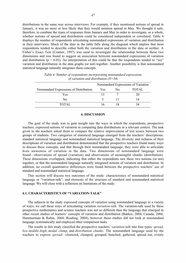
distributions in the same way across interviews. For example, if they mentioned notions of spread inJanuary, it was no more or less likely that they would mention spread in May. We thought it safe,therefore, to combine the types of responses from January and May in order to investigate, as a whole,whether notions of spread and distribution could be considered independent or correlated. Table 4displays the number of respondents articulating nonstandard expressions of variation and distributionin their interviews. Much of the data in the table falls along the diagonal which implies that mostrespondents tended to describe either both the variation and distribution in the data or neither. AFisher’s Exact Test (Cramer, 1997) was used to investigate the relationship between these twodimensions and was found to suggest an association between nonstandard expressions of variationand distribution (p = 0.02). An interpretation of this could be that the respondents tended to “see”variation and distribution in the data graphs (or not) together. Another possibility is that nonstandardstatistical language naturally integrates these concepts.

Table 4. Number of respondents incorporating nonstandard expressionsof variation and distribution (N=34)

Nonstandard Expressions of Variation

Nonstandard Expressions of Distribution Yes No TOTAL

Yes 13 7 20

No 3 11 14

TOTAL 16 18 34

6. DISCUSSION

The goal of the study was to gain insight into the ways in which the respondents, prospectiveteachers, expressed notions of variation in comparing data distributions in a relevant context. The taskgiven to the teachers asked them to compare the relative improvement of test scores between twogroups of students. Two categories of statistical language emerged from the teachers’ descriptions:standard statistical language and nonstandard statistical language. The diversity and richness of theirdescriptions of variation and distribution demonstrated that the prospective teachers found many waysto discuss these concepts, and that through their nonstandard language, they were able to articulatekeen awareness of variation in the data. Two dimensions of nonstandard language werefound—observations of spread (variation) and observations of meaningful chunks (distribution).These dimensions overlapped, indicating that either the respondents saw these two notions (or not)together, or that the nonstandard language naturally integrated notions of variation and distribution. Inaddition, no overall quantitative differences were found between the prospective teachers’ use ofstandard and nonstandard statistical language.

This section will discuss two outcomes of the study: characteristics of nonstandard statisticallanguage or “variation-talk”, and elements of the structure of standard and nonstandard statisticallanguage. We will close with a reflection on limitations of the study.

6.1. CHARACTERISTICS OF “VARIATION-TALK”

The subjects in the study expressed concepts of variation using nonstandard language in a varietyof ways; we call these ways of articulating variation variation-talk. The variation-talk used by theseprospective mathematics and science teachers was not so different than the language that emerged inother recent studies of learners’ concepts of variation and distribution (Bakker, 2004; Canada, 2004;Hammerman & Rubin, 2004; Reading, 2004), however these studies did not look at nonstandardlanguage systematically and employed other comparison tasks.

The results in this study classified the prospective teachers’ variation-talk into four types: spread,low-middle-high, modal clump, and distribution chunks. The nonstandard language used by theteachers to express spread—clustered, clumped, grouped, bunched, gathered, spread out, evenly

48

distributed, scattered, dispersed—all past participles, highlighted their attention to more spatialaspects of the distribution. These terms took on a meaning that implied attention to variation as acharacteristic of shape rather than as a measure. This is consistent with Bakker’s (2004) description ofshape as a pattern of variability. In contrast, concepts of variation in conventional statistical languageare articulated by terms like range or standard deviation, both of which are measures.

The other three types of “variation-talk”, all nouns, focused on aspects of the variability of thedata which required the prospective teachers to partition the distribution and examine a subset, orchunk of the distribution. Similar to Hammerman and Rubin’s (2004) teachers, the prospectiveteachers in this study simplified the complexity of the data’s variability by partitioning them into binsand comparing slices of data, in this case three slices: low-middle-high. Although simple, this is amore variation-oriented perspective than responses that took into account only the proportion ornumber of students who improved on the test. This approach is consistent with the findings of Bakker(2004), who argued that partitioning distributions into triads may be more intuitive than the moreconventional partitioning into four, as in the box plot. The awareness of learners’ tendency to simplifythe complexity of the data into low-middle-high bins motivated the creators of Tinkerplots (Konold &Miller, 2004) to include the “hat plot” (Konold, 2002) in the software, a representation where userscan partition the data into thirds based on the range, the average or standard deviation, the percentageof points, or a visual perspective of the data.

In some excerpts, teachers argued that the overlap of the middle slices was evidence that theEnrichment class was not effective. The focus on the modal clump (Konold et al., 2002) in data hasbeen a consistent finding across several studies of both students and teachers, reinforcing both theintuitive nature of seeing variability through slices-in-thirds, and recognizing the potential of using thenotion of a modal clump to encourage learners to move from a focus of individual points towards afocus on the aggregate of a distribution. Having a lens of a distribution as an aggregate, as opposed toa set of individual points, allows for concepts such as center to be thought of as a characteristic of thedistribution rather than as a calculation derived from individual points (Bakker, 2004). In addition,locating a modal clump allows the learner to simultaneously express their visualization of the centerand spread of the data (Konold et al., 2002), again highlighting its relational nature.

Finally, the use of other meaningful chunks by several of the prospective teachers demonstratedtheir ability to focus on the variability of the data by examining particular subsets of the distribution.This category contained responses as simple as comparing the outliers of one distribution to the“majority” of the other. A more complex visualization of distribution subsets was articulated byCarmen who used several different distribution subsets, with dynamic borders, as evidence for theeffectiveness of the Enrichment program. Her facility to fluidly manipulate borders of these subsetshighlighted her ability to visualize variation in the data. In addition, each of her meaningful chunkswas tied back to the context of the problem, indicating that she was able to use them to make meaningof the situation. Although Konold and Bakker have encouraged the conceptualization of a distributionas an aggregate, the articulation of distribution chunks by these teachers suggests that they arethinking of distribution chunks as mini-aggregates of the data. Kosslyn (1994) argues that our mindsand eyes work together to actively group input into perceptual units that ascribe meaning. We wouldargue that in articulating subsets of the distribution, the prospective teachers are communicating theperceptual units they are seeing in the data.

The three perspectives of seeing partial distributions—triads, modal clump, and distributionchunks—indicate that there are more than just the two perspectives of distribution that are usuallydiscussed in the literature: single points and aggregate. This third perspective—partial distributions or“mini-aggregates”—deserves further research to investigate the strength of its link to statisticalthinking about distributions. This study has highlighted that prospective teachers may use descriptionsof partial distributions not only to articulate rich views of variation, but also to use these distributionchunks in meaningful ways that could not be captured using conventional statistical terminology.Even though we classified expressions of variation separately from notions of distribution, thisseparation was somewhat artificial in that all four types of “variation-talk” expressed a relationshipbetween variation and distribution.

49

6.2. THE STRUCTURE OF STANDARD AND NONSTANDARD STATISTICALLANGUAGE

The nonstandard language used by the prospective teachers by its very nature integrates theimportant statistical ideas of variation and distribution, capturing and implying cognitive relationshipsbetween notions of center, dispersion, and shape. In contrast, the standard statistical language used bythe prospective teachers was by its very nature less relational, with a tendency to express importantideas in statistics as conceptually separate. Terms such as mean, standard deviation, and skeweddistribution describe the center, dispersion, and shape of a distribution but they do so in isolation. Theoveruse of this standard terminology, at least early in learning statistical concepts, may encouragelearners to maintain a perspective that statistical concepts are isolated “bits” of knowledge rather thaninformation that can provide insight into relationships in the data. Several difficulties of learningstatistics that are documented in research are consistent with a perspective of statistics as isolatedfacts. For example, seeing data as a set of isolated points rather than developing a “propensityperspective” (Konold, Pollatsek, Well, & Gagnon, 1997), lack of intuition in stochastics(Shaughnessy, 1992), or focusing instruction on calculations, isolated procedures, and graphcharacteristics in statistics instead of on drawing meaningful conclusions from data (Pfannkuch et al.,2004) may all be reinforced by the overuse (too much, too soon) of conventional statistical language.

The process of integrating rather than separating concepts in statistics has been shown to be aproductive avenue for developing statistical thinking and reasoning (Konold et al., 2002; Konold &Pollatsek, 2002; Bakker, 2004). This does not imply that one should “teach” nonstandard statisticallanguage as a means to encourage the development of students’ intuition about statistics, but rather toencourage their sense-making by acknowledging and encouraging learners’ own language. Had weacknowledged only conventional terms in our search for their articulation of variation, we would havelost many opportunities to gain insight into their thinking. For example, only two preservice teachersused the term “standard deviation” in their comparisons, and it can be argued that neither one usedthis concept to articulate meaning about variation.

An important lesson we learned in trying to categorize the preservice teachers’ descriptions washow difficult it was to separate their observations of variation and distribution. For example, whenApril described the shape of one distribution (“skewed to the left”), she compared its shape with thespread of the other distribution (“evenly spread out”). Using the teachers’ words, we could see thatdescribing data as clumped or spread out said as much about the distribution of the data as it didabout its variation. It was not surprising, therefore, when the responses in the two dimensions ofnonstandard language (variation and distribution) were found to be correlated.

6.3. LIMITATIONS OF THE STUDY

Although we believe that the results of this study communicate a powerful message about theopportunities of listening to learners’ nonstandard statistical language, several limitations of the studymust be acknowledged.

• Population. The subjects in the study were prospective secondary mathematics and scienceteachers and the study is not directly generalizable beyond that population. While many of theresults may seem to transfer to other groups (for example, practicing teachers), more researchwould need to be conducted in order to corroborate these results with other populations.

• Particulars of the task. The setting may have had strong influences on the responses that theprospective teachers gave during their interviews. Although the data were authentic, the taskwas not as it did not emerge from the teachers’ own desire to know. Therefore, it is possiblethat the responses given by the prospective teachers may have mirrored an expectation of whatthey thought the researchers wanted them to say, particularly since the researchers were alsotheir course instructors and the interviews were conducted as part of the course assessment.

• Particulars of the graphic. Elements of the graph could elicit responses that may differ withslight modifications. Recall, for example, that the means were marked on the figure andexplicitly pointed out to the subjects at the beginning of the task. By drawing specific attention

50

to the means, we may have been tacitly communicating that the means should have beenattended to in addition to or even instead of the prospective teachers’ own way of comparingthe two groups. The results of the Hammerman and Rubin (2004) study, for example, noted thatthe teachers in their study were not interested in using means to compare distributions butinvented their own ways of making meaning of comparisons in the problems they werediscussing.

• Irregularities in questioning. In a few of the interviews, the interviewer did not explicitly askfor a decision to be made regarding the effectiveness of the Enrichment program. This meantthat comparisons could not be made systematically regarding the prospective teachers’ use ofevidence towards a decision, which could have elicited richer responses.

• Generalizations about the course. Given the unique nature of the course which the prospectiveteachers undertook, the study was not designed to make generalizations about the effectivenessof such a course in developing learners’ statistical reasoning. Many of the compelling elementsused in the course and the task were developed from local problems in the implementation ofstandardized testing. Instead, the study was designed to focus on variation-related language thatpreservice teachers use at different stages or levels of learning about statistics. Other reports ofthe larger research study communicate elements of the course that may have had an impact onthe prospective teachers’ thinking and learning (Confrey et al., 2004; Makar & Confrey,submitted; Makar, 2004).

7. CONCLUSION AND IMPLICATIONS

This study was built on pioneering work by researchers at TERC who first studied teachers’nonstandard statistical language (e.g., Russell & Mokros, 1990), and shows the breadth and depth ofnonstandard language used by prospective teachers to describe variation. It follows that teachers needto learn to recognize and value “variation-talk” as a vehicle for students to express meaningfulconcepts of variation and distribution. This study has contributed to our understanding that preserviceteachers majoring in math and science often articulate meaning in statistics through the use of lessconventional terminology. Other research studies have shown that school children do so as well (e.g.,Bakker, 2004; Reading, 2004; Konold et al., 2002). These studies have begun to articulate rich andproductive learning trajectories to move students towards a more distribution-oriented view of data.

Although the preservice teachers in this study were using nonstandard statistical language, theconcepts they are discussing are far from simplistic and need to be acknowledged as statisticalconcepts. Not recognizing nonstandard statistical language can have two pernicious effects. For one,we miss opportunities to gain insight students’ statistical thinking. Noss and Hoyles (1996) explainthe benefits of attending to students’ articulation for creating mathematical meaning: “It is thisarticulation which offers some purchase on what the learner is thinking, and it is in the process ofarticulation that a learner can create mathematics and simultaneously reveal this act of creation to anobserver” (p. 54, italics in original). Gaining insight into student thinking, therefore, is not the onlybenefit from attending to nonstandard statistical language. Noss and Hoyles also argue that throughthe process of articulation, students have opportunities to create meaning. Sense-making in statisticsis an ultimate goal that is often neglected by more traditional learning environments. Valuing thediversity of students’ “variation-talk” and listening to student voice (Confrey, 1998) may encourageteachers to shift from the typically procedure-focused statistics courses towards a focus on sense-making. This is an issue of equity if we are to acknowledge the diversity of students’ ideas rather thanjust cover the content and label those who don’t talk statistically as being unable to do so.

The other problematic effect of neglecting students’ nonstandard statistical language is the tacitmessage that is communicated that statistics can only be understood by those who can use properstatistical talk. Lemke (1990) argues that the formal dialogue of science communicates a mystique ofscience as being much more complex and difficult than other subjects, requiring that we defer ourown ideas to those of ‘experts’. By doing so, Lemke argues

51

The language of classroom science sets up a pervasive and false opposition between a world ofobjective, authoritative, impersonal, humorless scientific fact and the ordinary, personal world ofhuman uncertainties, judgments, values, and interests … many of the unwritten rules about howwe are supposed to talk science make it seem that way (p. 129).

Although Lemke here is talking about science, the situation in statistics is isomorphic. Countlessstudents complain that statistics (which they call “sadistics”) is not understandable to ordinaryhumans and lacks a connection to sense-making. By communicating statistics as accessible only toexperts and geniuses, we are reinforcing a notion of statistics as a gatekeeper to powerful insightsabout the world, alienating students and denying opportunity to those who do lack the confidence intheir ability to make sense of statistics.

Three major benefits come out of teachers’ use of their own, nonstandard statistical terminologyin describing, interpreting, and comparing distributions. First, they are using words that hold meaningfor them and that convey their own conceptions of variation. In the constructivist perspective,knowledge is not conveyed through language but must be abstracted through experience. Nonstandardlanguage carries a subjective flavor that reminds us of this. Through interaction with others, thissubjectivity becomes intersubjective—one’s meaning is not identical to another’s, but through furtherexplanation, our meanings become more compatible with the language of our peers (von Glasersfeld,1991). Second, everyday uses of language are more accessible to a wide variety of students, allowingmultiple points of entry to statistical concepts while encouraging teachers to be more sensitive tohearing rich conceptions of variation in students’ voice (Confrey, 1998), words that may allowstudents easier access to class discussions. This is a more equitable, more inclusive stance; one that iscontrary to the conception of mathematics (or statistics) as a gatekeeper. Third, if the goal is toprovide students with experiences that will provide them with a more distribution-oriented view ofdata, then nonstandard statistical language that emerges from making meaning of statistical conceptsmay help to orient students (and their teachers!) towards this perspective. Describing a distribution as“more clumped in the center” conveys a more distribution-oriented perspective in language thanstating, say, standard deviation or range to compare its dispersion.

The results of this study are not meant to downplay the importance of using conventional termsand measures in comparing groups. On the contrary, these are very important tools. Our hope is thatteachers do not emphasize simply summarizing or reducing the data with conventional measures tomake overly simplistic comparisons as we have seen schools do in examining test data (Confrey &Makar, 2005), but rather seek insights into the context the data represent through richer views thatinclude notions of distribution and variation. Further research is needed to gain insight into howteachers understand concepts of variation and distribution, as well as to document how teacherssupport their students’ emerging statistical understanding.

ACKNOWLEDGEMENTS

This research was funded by the National (U.S.) Science Foundation under their Collaborative forExcellence in Teacher Preparation program (DUE-9953187). The authors are grateful to NSF for itsfinancial support and to the UTeach program at the University of Texas for their support in this study.The authors wish to thank the organizers of SRTL-3 for their permission and encouragement to makethese results available to a broader audience, and also appreciated the feedback offered by our SRTLcolleagues. The authors would also like to thank the reviewers who provided constructive, thoughtful,and extensive feedback on earlier drafts of this paper. Insightful and tenacious feedback from IddoGal, going beyond his role as editor of SERJ, greatly improved the final version.

52

REFERENCES

Bakker, A. (2004). Design research in statistics education: On symbolizing and computer tools.Published Doctoral dissertation. Utrecht, The Netherlands: Freudenthal Institute. [Online:www.stat.auckland.ac.nz/~iase/publications/dissertations/dissertations.php]

Bakker, A., & Gravemeijer, K. P. E. (2004). Learning to reason about distribution. In D. Ben-Zvi & J.Garfield (Eds.), The challenge of developing statistical literacy, reasoning, and thinking (pp. 147-168). Dordrecht, the Netherlands: Kluwer Academic Publishers.

Biehler, R. (1997). Student’s difficulties in practicing computer-supported data analysis: Somehypothetical generalizations from results of two exploratory studies. In J. Garfield & G. Burrill(Eds.), Research on the role of technology in teaching and learning statistics (pp. 169-190).Voorburg, The Netherlands: International Statistics Institute.

Boaler, J. (1997). Experiencing school mathematics: Teaching styles, sex, and setting. Buckingham:Open University Press.

Canada, D. (2004). Preservice teachers’ understanding of variation. Unpublished doctoraldissertation, Portland State University, Portland, Oregon (USA). [Online:www.stat.auckland.ac.nz/~iase/publications/dissertations/dissertations.php]

Cobb, P. (1999). Individual and collective mathematical development: The case of statistical dataanalysis. Mathematical Thinking and Learning, 1(1), 5-43.

Confrey, J. (1998). Voice and perspective: Hearing epistemological innovation in students’ words. InM. Larochelle, N. Bednarz, & J. Garrison (Eds.), Constructivism and education (pp. 104-120).New York, N.Y.: Cambridge University Press.

Confrey, J., & Makar, K. (2002). Developing secondary teachers’ statistical inquiry throughimmersion in high-stakes accountability data. In D. S. Mewborn, P. Sztajn, D. Y. White, H. G.Wiegel, R. L. Bryant, & K. Nooney (Eds.), Proceedings of the Twenty-fourth Annual Meeting ofthe North American Chapter of the International Group for the Psychology of MathematicsEducation (PME-NA), Athens, GA, (Vol. 3, pp. 1267-1279). Columbus, OH: ERIC Clearinghouse,Mathematics and Environment Education.

Confrey, J., & Makar, K. (2005). Critiquing and improving the use of data from high-stakes tests withthe aid of dynamic statistics software. In C. Dede, J. Honan, & L. Peters (Eds.), Scaling up forsuccess: Lessons from technology-based educational improvement (pp. 198-226). Cambridge,MA: Harvard College of Education.

Confrey, J., Makar, K., & Kazak, S. (2004). Undertaking data analysis of student outcomes asprofessional development for teachers. International Reviews on Mathematical Education(Zentralblatt für Didaktik der Mathematik), 36(1), 32-40.

Cramer, D. (1997). Basic statistics for social research. London: Routledge.

Finzer, W. (2001). Fathom! (Version 1.16) [Computer Software]. Emeryville, CA: Key CurriculumPress.

Fischbein, E. (1987). Intuition in mathematics and science: An educational approach. Dordrecht, TheNetherlands: D. Reidel Publishing Company.

Flyvbjerg, B. (2001). Making social science matter: Why social inquiry fails and how it can succeedagain. Cambridge, UK: Cambridge University Press.

Hammerman, J., & Rubin, A. (2004). Strategies for managing statistical complexity with newsoftware tools. Statistics Education Research Journal, 3(2), 17-41. [Online:www.stat.auckland.ac.nz/serj]

Hancock, C., Kaput, J. J., & Goldsmith, L. T. (1992). Authentic inquiry into data: Critical barriers toclassroom implementation. Educational Psychologist, 27(3), 337-364.

Hawkins, A. (Ed.). (1990). Teaching teachers to teach statistics. Voorburg, The Netherlands:International Statistics Institute.

Konold, C. (2002). “Hat Plots? ” Unpublished manuscript, University of Massachusetts, Amherst.

53

Konold, C., & Higgins, T. (2002). Highlights of related research. In S. J. Russell, D. Schifter, & V.Bastable, Developing mathematical ideas: Working with data, (pp. 165-201). Parsippany, NJ:Dale Seymour Publications.

Konold, C., Higgins, T., Russell, S. J., & Khalil, K. (submitted). Data seen through different lenses.Journal for Research in Mathematics Education.

Konold, C., & Miller, C. (2004). Tinkerplots (Version 1.0) [Computer Software]. Emeryville, CA:Key Curriculum Press.

Konold, C., & Pollatsek, A. (2002). Data analysis as the search for signals in noisy processes. Journalfor Research in Mathematics Education, 33(4), 259-289.

Konold, C., Pollatsek, A., Well, A., & Gagnon, A. (1997). Students analyzing data: research ofcritical barriers. In J. Garfield & G. Burrill (Eds.), Research on the role of technology in teachingand learning statistics (pp. 151-167). Voorburg, The Netherlands: International StatisticsInstitute.

Konold, C., Robinson, A., Khalil, K., Pollatsek, A., Well, A., Wing, R., & Mayr, S. (2002). Students’use of modal clumps to summarize data. In B. Phillips (Ed.), Proceedings of the SixthInternational Conference on Teaching Statistics, Cape Town, South Africa [CD-ROM]. Voorburg,The Netherlands: International Statistical Institute.

Kosslyn, S. (1994). Elements of graph design. New York: W. H. Freeman and Company.

Lemke, J. (1990). Talking science: Language, learning, and values. Norwood, NJ: Ablex Publishing.

Makar, K. (2004). Developing statistical inquiry: Prospective secondary mathematics and scienceteachers’ investigations of equity and fairness through analysis of accountability data.Unpublished Doctoral dissertation, University of Texas at Austin (USA). [Online:www.stat.auckland.ac.nz/~iase/publications/dissertations/dissertations.php]

Makar, K., & Confrey, J. (submitted). Modeling fairness in student achievement in mathematics usingstatistical software by preservice secondary teachers. ICMI Study Volume 14: Applications andmodeling in mathematics education.

Makar, K., & Confrey, J. (2004). Secondary teachers’ reasoning about comparing two groups. In D.Ben-Zvi & J. Garfield (Eds.), The challenges of developing statistical literacy, reasoning, andthinking (pp. 353-373). Dordrecht, the Netherlands: Kluwer Academic Publishers.

Marshall, J., Makar, K., & Kazak, S. (2002). Young urban students’ conceptions of data uses,representation, and analysis. In D. S. Mewborn, P. Sztajn, D. Y. White, H. G. Wiegel, R. L.Bryant, & K. Nooney (Eds.), Proceedings of the Twenty-fourth Annual Meeting of the NorthAmerican Chapter of the International Group for the Psychology of Mathematics Education(PME-NA), Athens, GA, (Vol. 3, pp. 1293-1304). Columbus, OH: ERIC Clearinghouse,Mathematics and Environment Education.

McClain, K. (2002). Supporting teachers’ understanding of statistical data analysis: Learningtrajectories as tools for change. In B. Phillips (Ed.), Proceedings of the Sixth InternationalConference on Teaching Statistics, Cape Town, South Africa [CD-ROM]. Voorburg, TheNetherlands: International Statistical Institute.

Moore, D. (1990). Uncertainty. In L. A. Steen (Ed.), On the shoulders of giants (pp. 95-137).Washington, D.C.: Academy Press.

Moore, D., & McCabe, G. (1993). Introduction to the practice of statistics (2nd ed.). New York:Freeman.

National Research Council (1999). High stakes: Testing for tracking, promotion, and graduation.Heubert, J. P., & Hauser, R. M. (Eds.), Washington, D.C.: National Academy Press.

National Research Council (2000). Inquiry and the National Science Education Standards: A guidefor teaching and learning. Washington, D.C.: National Academy Press.

National Research Council (2001). Knowing what students know. Washington, D.C.: NationalAcademy Press.

54

Noss, R., & Hoyles, C. (1996). Windows on mathematical meanings: Learning cultures andcomputers. Dordrecht, The Netherlands: Kluwer Academic Publishers.

Pfannkuch, M., & Begg, A. (2004). The school statistics curriculum: Statistics and probabilityeducation literature review. Mathematics Curriculum Reference Group Report to the Ministry ofEducation. Auckland, New Zealand.

Pfannkuch, M., Budgett, S., Parsonage, R., & Horring, J. (2004). Comparison of data plots: Building apedagogical framework. Paper presented at the Tenth International Congress on MathematicsEducation (ICME-10), Copenhagen, Denmark, 4-11 July.

Reading, C. (2004). Student description of variation while working with weather data. StatisticsEducation Research Journal, 3(2), 84-105. [Online: www.stat.auckland.ac.nz/serj]

Reading, C., & Shaughnessy, J. M. (2004). Reasoning about variation. In D. Ben-Zvi & J. Garfield(Eds.), The challenge of developing statistical literacy, reasoning and thinking (pp. 201-226).Dordrecht, The Netherlands: Kluwer Academic Publishers.

Russell, S. J., & Mokros, J. R. (1990). What’s typical: Teacher’s descriptions of data. Paper presentedat the Annual Meeting of the American Educational Research Association, Boston, MA.

Schoenfeld, A. (1991). On mathematics as sense-making: An informal attack on the unfortunatedivorce of formal and informal mathematics. In J. Voss, D. Perkins, & J. Segal (Eds.), Informalreasoning and education (pp. 311-343). Hillsdale, NJ: Lawrence Erlbaum Associates.

Shaughnessy, J. M. (1992). Research in probability and statistics: Reflections and directions. In D. A.Grouws (Ed.), Handbook of research on mathematics teaching and learning (pp. 465-494). NewYork: MacMillan.

Shaughnessy, J. M. (2001). Draft of grant proposal sent to the National Science Foundation.

Shaughnessy, J. M., Watson, J., Moritz, J., & Reading, C. (1999, April). School mathematicsstudents’ acknowledgement of statistical variation. In C. Maher (Chair), There’s More to Life thanCenters. Presession Research Symposium, 77th Annual National Council of Teachers ofMathematics Conference, San Francisco, CA.

von Glasersfeld, E. (Ed.) (1991). Radical constructivism in mathematics education. Dordrecht, theNetherlands: Kluwer Academic Publisher.

Watkins, A. E., Scheaffer, R., & Cobb, G. (2003). Statistics in action: Understanding a world of data.Emeryville, CA: Key Curriculum Press.

Watson, J., & Moritz, J. B. (1999). The beginning of statistical inference: Comparing two data sets.Educational Studies in Mathematics, 37, 145-168.

KATIE MAKAR

School of Education, Social Sciences Bldg

University of Queensland

Brisbane, Queensland 4072

Australia