Ann. Inst. Statist. Math. Vol. 57, No. 2, 279-290 (2005) Q2005 The Institute of Statistical Mathematics

VARIANCE ESTIMATION FOR SAMPLE QUANTILES USING THE m OUT OF n BOOTSTRAP

K. Y. CHEUNG AND STEPHEN M. S. LEE*

Department of Statistics and Actuarial Science, The University of Hong Kong, Pokfulam Road, Hong Kong, China, e-maih celiacky@graduate.hku.hk; smslee@hkusua.hku.hk

(Received January 21, 2004; revised May 7, 2004)

A b s t r a c t . We consider the p rob lem of e s t ima t ing the var iance of a sample quan- t i le ca lcula ted from a r a n d o m sample of size n. The r - th -o rde r kerne l - smoothed b o o t s t r a p es t ima tor is known to yield an impressively small re lat ive error of order 0(n-~/(2~+1)). It nevertheless requires s t rong smoothness condi t ions on the under ly- ing densi ty function, and has a per formance very sensi t ive to the precise choice of the bandwid th . The unsmoothed b o o t s t r a p has a poorer re la t ive error of order O(n-1/4), but works for less smooth dens i ty functions. We invest igate a modif ied form of the boo t s t r ap , known as the m ou t of n boo t s t r ap , and show tha t it yields a relat ive error of order smaller t h a n O(n -1/4) under the same smoothness condi t ions required by the convent ional unsmoothed b o o t s t r a p on the dens i ty function, provided t ha t the b o o t s t r a p sample size m is of an app rop r i a t e order. The e s t ima to r pe rmi t s exact , s imulation-free, compu ta t ion and has accuracy fairly insensi t ive to the precise choice of m. A s imula t ion s tudy is r epo r t ed to provide empir ica l compar ison of the various methods .

Key words and phrases: m out of n boo t s t r ap , quanti le , smoothed boo t s t r ap .

i . Introduction

Suppose that X1,. �9 �9 Xn constitute a random sample of size n taken from a distri- bution F. Let X(j) denote the j - th smallest datum in the sample. For a fixed p E (0, 1), assume that F has a continuous and positive density f on F -1 (O) for an open neighbour- hood O containing p. Denote by ~p = F-l(p) the unique p-th quantile of F . The p-th sample quantile X(r) is a natural and consistent estimator for ~p, where r = [np] + 1 and

2 Var(X(r)) [-] denotes the integer part function. Standard theory establishes that a n - admits an asymptotic expansion

(1.1) 2 = n-lp(1 p)f(~p)-2 +o(n-1). 6r n

A general discussion can be found in Stuart and Ord ((1994), w Although (1.1) provides an explicit leading term useful for approximating a2~, its direct computation requires the value of f(~p), which is usually unknown and is difficult to estimate. The conventional, n out of n, unsmoothed bootstrap draws a large number of bootstrap

2 by the sample variance of samples, each of size n, from X 1 , . . . , Xn, and estimates a n

*Supported by a grant from the Research Grants Council of the Hong Kong Special Administrative Region, China (Project No. HKU 7131/00P).

279

280 K . Y . C H E U N G A N D S T E P H E N M. S. L E E

the bootstrap sample quantiles calculated from the bootstrap samples. Hall and Martin (1988) show that the theoretical n out of n bootstrap estimator ^ 2 which is based on a n , infinite simulation of bootstrap samples, has an explicit expression

n

(1.2) an̂ 2 = Z ( X ( j ) _ X(r))2Wn,j, j = l

^ 2 has a large relative where Wn,j = r(n) I'i/n xr- l (1 - x)n-rdx. They prove that a n J( j -1) /n error of order O(n-1/4), that is an/a n ^ 2 2 _~ 1 + 0(n-1/4). Maritz and Jarret t (1978) note that ^ 2 may be more accurate than the leading term in the asymptotic formula a n (1.1) for p = 1/2 in small-sample cases, even if the true f(~p) is employed to calculate the latter. The smoothed bootstrap modifies the n out of n bootstrap procedure by drawing (smoothed) bootstrap samples from a kernel density estimate of f rather than from the empirical distribution of X 1 , . . . , Xn. Hall et al. (1989) show that the smoothed bootstrap estimator has a smaller relative error, of order O(n -r/(2r+l)) based on a kernel of order r, under much stronger smoothness conditions on f , provided that the smoothing bandwidth is chosen of order n -1/(2r+1).

The m out of n bootstrap, as pioneered by Bickel and Freedman (1981), provides a method for rectifying bootstrap inconsistency in many nonregular problems: see, for example, Swanepoel (1986) and Athreya (1987). It is, however, generally less efficient than the n out of n bootstrap when the latter is consistent: see, for example, Shao (1994) and Cheung et al. (2005). Exceptional cases have been found though. Wang and Taguri (1998) and Lee (1999) improve the n out of n bootstrap by suitably adjusting the resample size m in estimation and confidence interval problems respectively. Arcones (2003) shows that the n out of n bootstrap provides a consistent estimator for the distribution function of sample quantiles with error of order 0(n-1/4), whilst the m out of n bootstrap reduces the error to order O(n -1/3) by use of m (x n 2/3. Janssen et al. (2001) obtain independently similar results for U-quantiles. We shall show in the present context that the m out of n bootstrap is also effective in reducing the relative error of ^ 2 under the minimal smoothness conditions same as those required by the n out of n O" n

bootstrap on f . The rest of the paper is organized as follows. Section 2 reviews the smoothed boot-

strap method for variance estimation for sample quantiles. Section 3 studies the conver- gence rate, as well as the asymptotic distribution, of the m out of n bootstrap variance estimator. Section 4 describes a computational algorithm for empirically determining the optimal m. Section 5 presents a simulation study to compare the performances of the various variance estimators. Section 6 concludes our findings. Technical details are given in the Appendix.

2. Smoothed bootstrap

2 Instead of re- We review the smoothed bootstrap procedure for estimating a n . sampling from the empirical distribution of X 1 , . . . , X n , the smoothed bootstrap sim- ulates smoothed bootstrap samples from a kernel density estimate ]b of f , given by h ( x ) =(nb) -1 ~-]in=_l K( (x - X~)/b), where b > 0 denotes the bandwidth and K is an r-th-order kernel function for r _> 2. The smoothed bootstrap estimator an, b ^2 of an2 is then obtained by calculating the sample variance of the p-th-order smoothed bootstrap sample quantiles.

BOOTSTRAP VARIANCE ESTIMATION FOR QUANTILES 2 8 1

Let f(J) be the j - th -der iva t ive of f . Assume tha t f ( r ) exists and is uniformly continuous, f(J) is bounded for 0 ~_ j < r, f is bounded away from 0 in a ne ighbourhood of ~p and EIXI v < co for some ~ > 0. Then Hall et el. (1989) show tha t a~, b^2 has the

opt imal relative error of order 0(n-~/(2~+1)), achieved by set t ing b c~ n -1/(2~+1). In principle, the relative error can be made arbi t rar i ly close to O(n -1/2) by choosing a sufficiently high kernel order r.

It should be noted tha t when r > 2, ]b(X) necessarily takes on negative values for some x and poses pract ical difficulties if smoothed boo t s t r ap samples need be s imulated from lb. Negat ivi ty correct ion techniques of some sort must be incorpora ted into the smoothed boo t s t r ap procedure to make it computa t iona l ly feasible: see, for example, Lee and Young (1994). In the case where r = 2 so tha t ]b is a proper densi ty function, the opt imal relat ive error of 52b is of order 0(n-2 /5) , which a l ready improves upon the

unsmoothed n out of n boo ts t rap , which has a relat ive error of order O(n-1/4).

3. m out of n bootstrap

The m out of n boo t s t r ap modifies the n out of n boo t s t r ap by drawing boo t s t r ap samples of size m, instead of n, from the empirical d is t r ibut ion of X 1 , . . . , Xn, where m satisfies m = o(n) and m ~ co as n ---* co. The corresponding variance es t imator a m ^ 2 is then defined as m / n t imes the sample variance of the p- th boo ts t rap sample quantiles.

Recall tha t X(j) is the j - t h order stat ist ic of X 1 , . . . , X,~ and X(r) is the p- th sample quantile. The m out of n boo t s t r ap variance es t imator a m ^ 2 admits an explicit, d i rect ly computable , formula:

n

(3.1) a m 2̂ = (re~n) E ( X ( j ) - X(r))2wmj, j = l

where Wm,j = k(~) f~i/21)/n xk-1 (1--x)m-kdx and k = [mp]+l . Our main theorem below

establishes asympto t ic normal i ty of 5 2 together with the corresponding convergence rate. Its proof is out l ined in the Appendix.

THEOREM 3.1. Assume m oc n ~ for some ~ C (0, 1), ]EIXI v < co for some ~7 > O, f = F' exists and satisfies a Lipschitz condition of order v = �89 + ~, with E e (0, �89 in a neighbourhood of ~p, and f(~p) > O. Then

(3.2) n3/2m-1/4(52 m - - (T 2) = Sn -4- Op(ml /4n -1/2 -4- m-1 /2-e /2n l /2 ) ,

where Sn converges in distribution to N ( O , 2 ~ - l / 2 [ p ( 1 - p)]a/2f(~p)-4).

The expansion (3.2) enables us to deduce the opt imal choice of m by which ^ 2 (:7 m

achieves the fastest convergence rate, as is asserted in the following corollary.

COROLLARY 3.1. Under the conditions of Theorem 3.1, a m ^ 2 has an optimal relative error of order O(n-(l+2~)/(4+4E)), achieved by setting m c< n 1/(1+~).

Hall and Mar t in (1988) show tha t n5/4(52 n - a2n) has the same asympto t ic normal d is t r ibut ion as does n3/2m-1/4(6~m - a2n) under exact ly the same condit ions of Theo-

2 at a faster ra te t han does ~ 2 which has a rem 3.1. It is clear t ha t a m 2̂ converges to a n an,

282 K. Y. C H E U N G AND S T E P H E N M. S. LEE

relative error of order O(n -1/4). Although the smoothed boots t rap est imator an,b^2 has

an even smaller relative error, of order 0(n-~/(2~+1)), t han ^ 2 for any r > 2, it requires O" m

tha t f be at least twice continuously differentiable in a neighbourhood of ~p, a condit ion much stronger than those of Theorem 3.1. Moreover, tha t no such computable expres- sion as (3.1) exists for ^2 ^2 a~,b means tha t an, b has to be approximated by Monte Carlo simulation, which is computat ional ly more expensive and is not immediate ly feasible if r > 2 due to the problem of negativi ty of lb.

Arcones (2003) establishes versions of Theorem 3.1 and Corollary 3.1 for m out of n boots t rap est imation of the distr ibution of X(~). He shows, under the stronger assumption tha t f is differentiable at ~p, tha t the fastest convergence rate, of order n -1/3, is a t ta ined by setting m c< rt 2/3. Our results apply to the variance of X(~) and to densities f under less stringent smoothness conditions. Densities violating Arcones' but satisfying our smoothness conditions include those which are Lipschitz continuous of order u e (1/2, 1) near ~p. A simple example is f ( x ) = (7/6)(1 - Ixl3/4), for Ix[ < 1, which is Lipschitz continuous of order 3/4 at x = 0.

4. Empirical determination of m

It follows fi'om Corollary 3.1 tha t fixing m = cn ~, for some constants c and V independent of n, yields the best convergence rate for a m. ^ 2 In practice V is unknown and so is the opt imal value of c. We sketch below a simple algorithm, based on the bootstrap, for empirical determinat ion of bo th c and V and hence the opt imal choice of m.

First fix S distinct boots t rap sample sizes m l , . . . , m s < n, for some S > 2. For each s = 1 , . . . , S, calculate a .2 = ( n / m s ) 6 2 , the variance of the p-th boots t rap sample quantile induced by the drawing of boots t rap samples of size ms. Generate a large number, B say, of boots t rap samples X~*I,... , 2d~*B, each of size ms, from X 1 , . . . , Xn. For each X~*b, calculate the e out of ms est imate of a*2s , namely

ffs,b,e -~ (g /ms ) E ( X f f , ( j ) - ~'b,(r'))Y* ~21.*~ x k ' - I (1 -- X) e-k• dx, j = l J ( j - 1 ) / m .

where k* = [@] + 1, r* -- [msp] + 1 and X'b,(0 denotes the i - th smallest d a t u m in 2d*s,b. The mean squared error of the g out of m8 boots t rap variance es t imate is then es t imated by MSE~(g) B_I B ^,2 _ a~2)2 = E b = l ( a s , b , g . Select e = es which minimizes MSE~(e) over e E { 1 , . . . , ms }. Asymptot ical ly es ~ cm~, so t ha t log e, ~ log c + ~/log ms, for s = 1 , . . . , S. S tandard least squares techniques yield tha t c ~ exp{D -1 (M2L1 - M I K ) }

s ES_l(lOg and V ~ D - l ( S K - MIL1), where M1 = )-~s=l logms, M2 = ms) 2, L1 = S S )-~s=l log/s , K = ~s=l(logms)(loges) and D = SM2 - M 2. Finally calculate the

opt imal m to be m = [cn~], wi th c and 3' fixed at the above approximate values.

5. Simulation study

We conducted a simulation s tudy to compare the mean squared errors of 62, a m ^ 2 and an,b , ^ 2 for p = 0.1, 0.5 and 0.9 and for fixed values of m and b. Random samples of sizes n = 50 and 200 were generated from three distributions: (i) the s tandard normal distribution, N(0, 1), (ii) the chi-squared dis tr ibut ion with 5 degrees of freedom, X52, and (iii) the double exponential distr ibution with density function f ( x ) = (1 /2 )exp( - Ix l ) . All three distributions have densities satisfying the Lipschitz condit ion of order one, so tha t the

B O O T S T R A P V A R I A N C E E S T I M A T I O N F O R Q U A N T I L E S

p=0.1

p=0.5

p=0.9

rn out of n I n = 5 0 n out of n n=200

. . . . . . . . smoothed

0.003 0.0 0,5 1.0 1.5 2.0 0.0 0.5 1.0 1.5 2.0 2.5 b

0 . 0 0 0

0.0

0.0006

0.0006

0 .0004"

O.OOO2

0.0000

0.0

0.004

O.0O3

0.00~

0.001

0.000

c~ c~ [ 3 .

E]

/ /

I" l

--/.

/ s

�9 J �9

~ ~ c ~ B ~ : ~ �9 , ~ " �9 "

5

0.5

O.OCCO0 5 10 15 20

0.5 1.0 1.5 2.0 0.0

0.000025

0.000020

0.000015

0.00C010

O,OOOO05

m 0.000000 10 15 2O

1.0 1.5 2.0 0.0

% [D

& -

5 10 15

0.O0010

O.OOOO6

0.00006

0.00004

0.0C002

0.00000 2O

? I"

/ !

[]

m

20 40 60 80 100

0.5 1.0 1,5 2.0

[]

l /

/

i i

[]

/ ./"

20 40 60 80 100

0.5 1.0 1.5 2.0 2.5

D

I

i !

.[3 j

A.

20 40 60 80 100

Fig. 1. Normal Example : m e a n squared errors of &n ~, &2 m (p lot ted against m ) and an, bA 2 (p lot ted against b) for n -- 50 and 200, and p --- 0.1, 0.5 and 0.9.

2 8 3

conditions of Theorem 3.1 hold for e = 1/2. For the smoothed bootstrap estimator an,b , ^ 2 the second-order Epanechnikov kernel function k( t ) -- max{(3/4)(1 - t 2 ) , 0 } was employed. Note that the first derivative of the double exponential density function does not exist at ~0.5 = 0, so that the density there lacks the smoothness condition sufficient for proper functioning of the smoothed bootstrap method based on the kernel k above. Each smoothed bootstrap estimate ^2 an, b was derived from 1,000 smoothed bootstrap

samples. The estimates ^ 2 and ^ 2 a n a m were directly computed using explicit formulae (1.2) and (3.1) respectively. Each mean squared error was obtained by averaging over 1,600 random samples drawn from F.

Figure 1 plots the mean squared error of a m ^2 against m (bottom axis) and that of an,b̂ 2 against b (top axis) for the normal distribution. Similar comparisons for the chi- squared and double exponential distributions are given in Figs. 2 and 3 respectively. The mean squared error of a N ^ 2 is also included in each diagram for reference.

For the N(0, 1) data, as predicted from asymptotic results, the n out of n bootstrap yields for ^2 the largest mean squared error, except for cases of large b or m, for all a n

combinations of n and p. The mean squared error of the smoothed bootstrap estimate

284 K. Y. CHEUNG AND STEPHEN M. S. LEE

I �9 m out ol n I - - n out of ~ n = 2 0 0

n = 5 0 . . . . c - .... s, ,~ot,ed

0.0 0.5 , .0 , .5 2.0 2.5 3.0 0.0 0.5 ,.0 t.s 2.0 2 .~ b D 0.020

0.0005 /~

0.015 O 0.0004 I / :.

/" .,_,

0.010 ./" 0.0003 D /

�9 .1 0.0002 "/" p=0.1 0.005 D"D ~ D El. O �9 ~ �9

O "D �9149 " [ ~ D . D ' "~"A~ . �9 - �9 0.6O01 "~ ~ " [J

" ~v-& " �9 /

0,06O m 0.06O0 ( ~ 5 10 15 2O 20 40 6O 8O 100

or) E 0 2 4 6 1 2 3 4 5

b o6o \ /[] 0.00,2 ,i:? 0.114 0.0O08 I'

p--.-.~.s \ i ! / -

0.02 ~ 1 / 0.0004 [~ �9 �9 / ' �9 . " - - [3 ~. E2. "r ~ ~ : ~ ""

0,00 0.0000 m 5 10 15 20 20 40 60 80 100

0 2 4 6 8 10 12 14 0 2 4 6 8 10 12 b 4 b "

3 0.06 - - i

p=O.9 2 �9 0.04

1 0 .02 ,,.'"

. . D

0 0.00 m 0 5 10 15 20 20 40 60 80 100

Fig . 2. Ch i - squared E x a m p l e : m e a n squared errors of &2n, ~r2 m (p lo t t ed a g a i n s t m ) and ^2 O'n, b ( p l o t t e d aga ins t b) for n = 50 a n d 200 , a n d p = 0.1, 0 .5 a n d 0.9.

an,b ̂2 varies w i th b parabolical ly . A l t h o u g h it is a symptot i ca l ly less accurate, the rn out of

n b o o t s t r a p es t imate &2 m has m e a n squared error comparable to that of on, b ^ 2 cons truc ted

using an opt imal b, and mainta ins a more stable performance than O'n, b ^ 2 for n = 200. A m o n g the values of p studied, all three e s t imators tend to be m o s t accurate at p = 0.5 for b o t h n = 50 and 200.

For data drawn from the a s y m m e t r i c X52, the m e a n squared errors of the e s t imators are in general larger than those observed in the N ( 0 , 1) example , and increase as p increases. As in Fig. 1, we see from Fig. 2 that ^2 is general ly the least accurate , O" n while the m e a n squared errors of ^ 2 and ^ 2 o m O'n, b a r e of similar magni tudes . The opt imal

choice of bandwidth , which yields the m i n i m u m m e a n squared error for ~Tn,b, ^ 2 increases

cons iderably as p increases; the opt imal choice of m for o" m ^ 2 , by constrast , s tays wi th in the s a m e range as p varies, rendering its empirical de terminat ion less difficult than that of the opt imal bandwidth .

Figure 3 displays the findings for the double exponent ia l data. For p = 0.1 and 0.9, we see that an, b ^ 2 and o- m ^ 2 have comparab le m e a n squared errors, which are no tab ly smal ler

than that of an, ^ 2 provided b and m are se lected sensibly. For p = 0.5, the m e a n squared

BOOTSTRAP VARIANCE ESTIMATION FOR QUANTILES

0.08

0.06

p=0.1 0.04

0.02

0.00

0.0

0.0012

0.0008

p=O.5 0.0004 . . . . .

p=0.9

0.08

0.06

0.04

0.02

0.00

=::= mouo, o] n = 5 0 . out of n n = 2 0 0

smoothed

0 1 2 3 4 5 1 2 3 4 b b

j / �9 " B - - 7

El[][:] A I � 9 CJ �9 [~ �9 [ ] [ ] [ ] " .~.'"

�9 . ~, . [ ] . [ ]

5 10 15 20

0.5 1.0 1.5

E3

../ �9 /"

[] ._ [] . ' - - r � 9 � 9

_1 0.0025

0.0020

0.0015

0.0010

0.0005

0.0000,

0.0

0.00010

0.000~

0,00006

0.000O4

0.00~02

0.00000

b 0.0020

O.O015

0.0010

0.0005

m 0.0000 20

�9 j � 9 1 4 9 D

. E3~[]C3C3 �9 N . 1~ E3

20 40 60 80 100

0.5 1.0 1.5 2.0

/[ ]

y/

[ 3

/ :

/ "

i ~

5 10 15 20 20 40 60 80 100

1 2 3 4 5 0 1 2 3 4

~ 3 O D O O D " O , r 7 ' D " ~

20 40 60 80 100

Fig. 3. Double Exponent ia l Example: mean squared errors of &2, ~2 m (plotted against m) and O.n, b^2 (plotted against b) for n = 50 and 200, and p = 0.1, 0.5 and 0.9.

285

^2 error of On, b ^ 2 increases significantly as b increases, and is much larger than those of a n

and a m ^ 2 for n = 200, due plausibly to the lack of s m o o t h n e s s of the double exponent ia l dens i ty at ~0.5 = 0. In general the m out of n boot s t rap performs much bet ter than the n out of n boot s trap for n = 200, except for a smal l m -- 9. Similar to the N ( 0 , 1) example , all three m e t h o d s are m o s t accurate at p -- 0.5 a m o n g the values of p studied.

We note that in m o s t of the invest igated cases the accuracy of the m out of n b o o t s t r a p deteriorates markedly for s o m e very smal l values of m. A heurist ic exp lanat ion is as follows. We see from the proof of T h e o r e m 3.1 that a s y m p t o t i c propert ies of a m ^2 depend critically on the weights Wmj for j c lose to r. L e m m a A.1 shows that the wm,j sequence, for j c lose to r, resembles a symptot i ca l ly the central shape of a normal density. Thus our a s y m p t o t i c findings can reliably predict f ini te-sample behav iour only w h e n the Wm,j atta ins its m o d e at some j strict ly be tween 1 and n. E x a m i n a t i o n of the wm,j in detai l shows that the latter condi t ion holds only w h e n m exceeds a certain value, M ( n , p) say, depending on bo th n and p. Under the set t ings of our s imula t ion study, we find that for b o t h n = 50 and 200, M ( n , p ) = 9, 2, 10 for p = 0.1, 0.5 and 0.9 respectively. Indeed Figs. 1 -3 all suggest that the m out of n boot s t rap per formance begins to stabi l ize once

286 K . Y . C H E U N G A N D S T E P H E N M. S. L E E

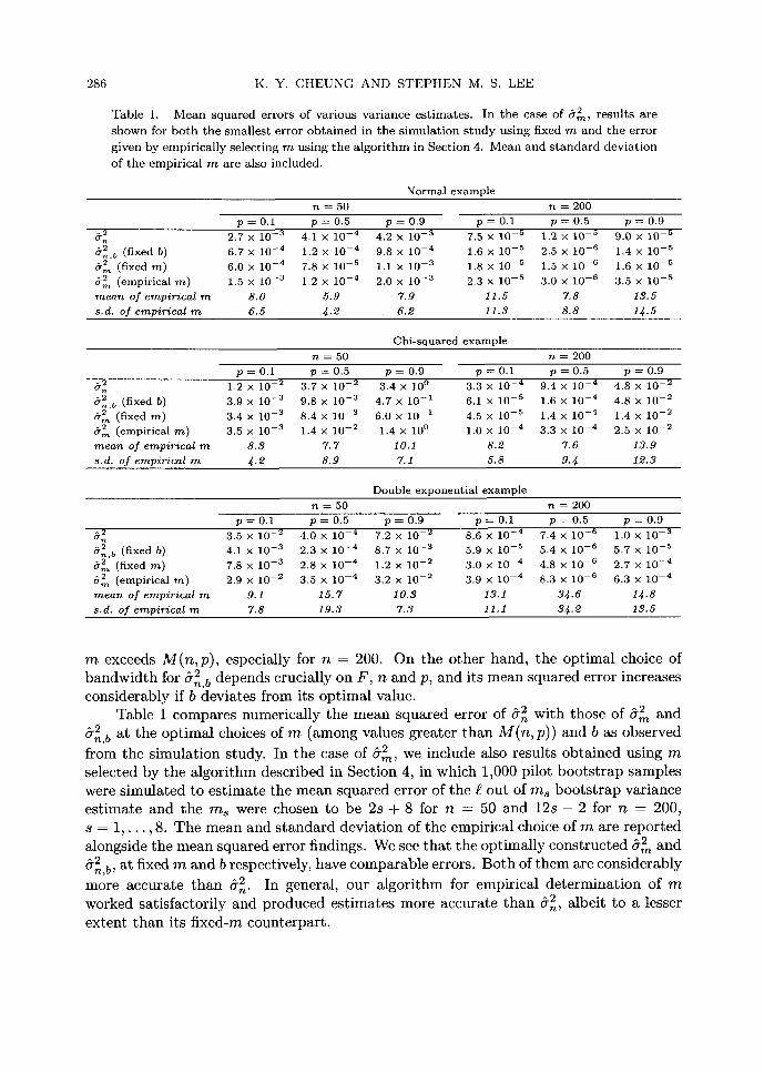
T a b l e 1. M e a n s q u a r e d e r r o r s o f v a r i o u s v a r i a n c e e s t i m a t e s . I n t h e c a s e o f &2m, r e s u l t s a r e

s h o w n fo r b o t h t h e s m a l l e s t e r r o r o b t a i n e d in t h e s i m u l a t i o n s t u d y u s i n g f ixed m a n d t h e e r r o r

g i v e n b y e m p i r i c a l l y s e l e c t i n g m u s i n g t h e a l g o r i t h m in S e c t i o n 4. M e a n a n d s t a n d a r d d e v i a t i o n

o f t h e e m p i r i c a l m a r e a l so i n c l u d e d .

N o r m a l e x a m p l e

n = 50 n = 200

p = 0 . 1 p : 0 . 5 p = 0 . 9 p = 0 . 1 p = 0 . 5 p = 0 . 9

(~2 2.7 • 10 - 3 4.1 • 10 - 4 4.2 • 10 - 3 7.5 • 10 - 5 1.2 • 10 - 5 9 .0 • 10 - 5

&~2b (f ixed b) 6.7 • 10 - 4 1.2 • 10 - 4 9.8 • 10 - 4 1.6 • 10 - 5 2.5 • 10 - 6 1.4 • 10 - 5

d ~ (f ixed m ) 6.0 • 10 - 4 7.8 • 10 - 5 1.1 • 10 - 3 1.8 • 10 - 5 1.5 • 10 - 6 1.6 • 10 - 5

~ ( e m p i r i c a l m ) 1.5 • 10 - 3 1.2 x 10 - 4 2.0 x 10 - 3 2.3 x 10 - 5 3.0 x 10 - 6 3.5 x 10 - 5

mean o f empirical m 8.0 5.9 7.9 11.5 7.8 13.5

s.d. o f empir ical m 6.5 4.2 6.2 11.3 8.8 14.5

C h i - s q u a r e d e x a m p l e

n = 50 n = 200

p = 0 . 1 p = 0 . 5 p = 0 . 9 p = 0 . 1 p = 0 . 5 p = 0 . 9

( ~ 1.2 x 10 - 2 3 .7 • 10 - 2 3.4 • 10 ~ 3.3 • 10 - 4 9.4 • 10 - 4 4.8 • 10 - 2

d 2 b (fixed b) 3.9 • 10 - 3 9.8 • 10 - 3 4.7 • 10 - 1 6.1 • 10 - 5 1.6 • 10 - 4 4.8 • 10 - 2

5 ~ (f ixed m ) 3.4 • 10 - 3 8.4 • 10 - 3 6.0 x 10 - 1 4.5 • 10 - 5 1.4 • 10 - 4 1.4 x 10 - 2

5 2 ( e m p i r i c a l m ) 3.5 • 10 - 3 1.4 • 10 - 2 1.4 • 10 ~ 1.0 • 10 - 4 3.3 • 10 - 4 2.5 • 10 - 2

mean o f empir ical m 8.3 7 . 7 10.1 8.2 7.6 13.9

s.d. o f empir ical m 4.2 8.9 7.1 5.8 9. 4 12.3

D o u b l e e x p o n e n t i a l e x a m p l e

n = 50 n = 200

p = 0 . 1 p = 0 . 5 p = 0 . 9 p = - 0 . 1 p = 0 . 5 p = 0 . 9

52 3.5 • 10 - 2 4.0 • 10 - 4 7.2 • 10 - 2 8.6 • 10 - 4 7.4 • 10 - 6 1.0 • 10 - 3

&2~, b (f ixed b) 4.1 • 10 - 3 2.3 • 10 - 4 8.7 • 10 - 3 5.9 • 10 - 5 5.4 • 10 - 6 5.7 • 10 - 5

&2 (fixed m ) 7.8 • 10 - 3 2.8 • 10 - 4 1.2 x 10 - 2 3.0 • 10 - 4 4.8 • 10 - 6 2 .7 • 10 - 4

~ 2 ( e m p i r i c a l m ) 2.9 x 10 - 2 3.5 • 10 - 4 3.2 • 10 - 2 3.9 • 10 - 4 8.3 • 10 - 6 6.3 x 10 - 4

mean o f empir ical m 9.1 15.7 10.3 13.1 34.6 14.8 s.d. o f empir ical m 7.8 19.3 7.3 11.1 34.2 13.5

m exceeds M(n,p), especially for n = 200. On the o ther hand, the op t ima l choice of b a n d w i d t h for an, b ^ 2 depends crucial ly on F , n and p, and its m e a n squared error increases cons iderably if b devia tes f rom its op t i m a l value.

Table 1 compares numerical ly the m e a n squared error of 5_2 wi th those of a m^ 2 and ~Tn, b^2 at the op t im a l choices of m (among values g rea te r t h a n M(n,p)) and b as observed

f rom the s imula t ion study. In the case of ^ 2 am, we include also results ob ta ined using m selected by the a lgor i thm descr ibed in Sect ion 4, in which 1,000 pilot b o o t s t r a p samples were s imula ted to e s t ima te the m e a n squared er ror of the g out of ms b o o t s t r a p var iance es t ima te and the ms were chosen to be 2s + 8 for n = 50 and 12s - 2 for n -- 200, s = 1 , . . . , 8. T h e m e a n and s t a n d a r d dev ia t ion of the empir ica l choice of m are r epo r t ed alongside the m e a n squared error findings. We see t h a t the op t imal ly cons t ruc ted a m ^ 2 and (Tn,b,̂ 2 at fixed m and b respectively, have c o m p a r a b l e errors. B o t h of t h e m are cons iderably

more accura te t h a n an. ^ 2 In general , our a lgor i thm for empir ica l de t e rmina t ion of m worked sat is factor i ly and p roduced es t ima tes more accura te t h a n a N ^ 2, albei t to a lesser extent t h a n its f ixed-m counte rpar t .

B O O T S T R A P V A R I A N C E E S T I M A T I O N F O R Q U A N T I L E S 287

6. Conclusion

We have shown, both theoretically and empirically, that the m out of n bootstrap variance estimator ~ ~ is notably superior to the conventional n out of n bootstrap estima- o,rn

^2 t o r a n.̂ 2 For densities satisfying a Lipschitz condition of order within (1/2, 1] near ~p, o.,~ incurs a relative error of smaller order than o.n,.. 2 provided that m is chosen appropriately. The smoothed bootstrap estimator 6~, b may yield an even smaller relative error using an optimal bandwidth b, but requires much stronger smoothness conditions on the density f . The rn out of n bootstrap therefore offers a convenient alternative which is more accurate than the n out of n bootstrap and more robust than the smoothed bootstrap. Under a smooth f for which both smoothed and uusmoothed bootstraps work properly, we have that o.n,A2 o'm 2̂ and o,n, b^2 generate relative errors of orders O ( n - I / 4 ) , O(n -~/3) and

O(n -2/5) respectively, provided that m o< n 2/3, b c( n -1/5 and a second-order kernel is used in constructing ^ 2 O-n, b �9

Our simulation results agree closely with the asymptotic findings. Both the smoothed and the m out of n bootstraps, when constructed optimally, yield compa- rable accuracies and outperform the n out of n bootstrap method substantially. The optimal choice of bandwidth for the smoothed bootstrap varies considerably with the problem settting. The mean squared error of o.n, b ^ 2 is also very sensitive to the bandwidth. A slight deviation from the optimal value of the bandwidth may greatly deteriorate the accuracy of the estimate. One therefore requires a sophisticatedly-designed, data- dependent, procedure for calculating the optimal bandwidth in practice. On the other hand, the observed mean squared error of 62 m remains relatively stable over awide range of m beyond M ( n , p), especially for large n. Also, the optimal choice of m tends to stay within a stable region which varies little with the problem setting. This suggests that the precise determination of m is less crucial an issue than is the choice of bandwidth for o ,n ,b" ^ 2 We have proposed a simple bootstrap-based algorithm for empirically determining the optimal m and obtained satisfactory results in our simulation study.

Unlike most bootstrap-based estimates, o. n ^ 2 and 6 2 can be evaluated directly using formulae (1.2) and (3.1) respectively, so that no Monte Carlo simulation is necessary, making their computation exact and very efficient. The smoothed bootstrap estimate O-n, b ^ 2 must, however, most conveniently be approximated using Monte Carlo simulation. Use of a higher-order kernel, which effects in an improved error rate, further complicates the Monte Carlo procedure due to negativity of the kernel estimate ]b-

Appendix

A.1 Proof of Theorem 3.1 The proof is modelled after Hall and Martin's (1988) arguments. Let r denote the standard normal density function, Yn,j = (j - 1 ) /n and bran =

(rny,,,y - k){my, , , j (1 - Y n , j ) } -1/2. The following lemma states a useful asymptotic ex- pansion for the weight Wm,y.

LEMMA A.1. Assume that m ~ n ~ for some A C (0, 1). There exists some constant C > 0 such that

Wm,j = m'/2n-1{Yn, j(1 - yn,j) }-U2r + O(n - ] e-Om(Y"J-P)2).

288 K. Y. CHEUNG AND STEPHEN M. S. LEE

PROOF. Note tha t wm,j = I j / n (k ,m - k + 1) - I ( j_ l ) /~(k ,m - k + 1), where

Iy(a,b) -- 5 -'a+b-1 (a+b-l)yJ(1 y)a+b-l-j Withou t loss of generality, consider j = np + q with q _> 0. ~he proof is completed by considering the Edgeworth expansion of the binomial distr ibution function for the case 0 <_ q <_ Dnm-1/2( lnm) 1/2, for some D > 0, and Bernstein's inequality for the case q > Dnm-1/2( lnm) 1/2. []

We first consider the summat ion over j in (3.1). The expansion for am 2̂ then follows trivially after multiplication by m/n. The summat ion is divided into two parts , for some (f > 0 and fl < A/12: (i) IJ - r] > 5nl+~m-1/2; and (ii) IJ - rl <- 5nl+~m-1/2.

For par t (i), we note tha t max{(X(j) - X(r)) 2 : j <_ n} <_ 4n 4/v in probability: see Hall and Mar t in (1988). Lemma A.1 implies that , for some constant C2 > 0, Wmj < C2ml/2n-le-Cm(ynJ-P)2. Thus, with probabili ty tending to one, we have tha t for some constant C3 > 0 and any ~ > 0,

(A.1) E (X(j) - X(r))2wm,j < 4 C2ml/2na/oe -Can2€ = O(n-r [j--rl>~nl+f~m-1/2

For part (ii), we assume throughout tha t IJ - r[ < ~nl+f~m-1/2, and tha t ~-~j refers to

summat ion over j satisfying the above, unless specified otherwise. Let H(x) = F - l (e -x) and I"1,---, Yn denote independent and identically dis t r ibuted exponential variables with unit mean. Define sj = s g n ( r - j ) , m0j = min ( r , j ) , mlj = m a x ( r , j ) - l , Ar = )-~n= r U -1.

1 Suppose t ha t f satisfies a Lipschitz condit ion of order v -- 7 + ~ in a neighbourhood of ~p, so tha t a - H'(A~) = _pf(~p)-I + O(n-1). Following Hall and Mart in ' s (1988) arguments, we have

(A.2) E ( X ( j ) - - X ( r ) ) 2 W m , j = S1 -~- $2 -~- T1 -~- T2 -~- T3, J

where S 1 = a 2 E j b2wm,j, $2 ---- 2a2 ~-~j bj(Bj - b j ) w m j , T1 = a 2 ~-~j(Bj -b j )2Wmj, T2 = 2 ~-]~j DjRljWm,j, T3 = ~'~j R21jWm,j, Bj = Eu=mojmlj u-lye, , bj -- E(Bj ) , Dj = 8jaBj,

Rl j = R2j + R3j, R2j = s jB j [g ' (A~ ) -a] and Raj = s jBj f l [g, ( A~ + ts jBj ) _ H, ( A~)]dt. Note also t ha t Br = br = 0 and tha t

(A.3) bj = [j - rl r - 1 § 2-1( j - r)2r -2 + O([ j - rlar-3).

Using L e m m a A.1 and (A.3), we have

(j-rS ll) E b2wm'j = rr~l/2n-l E k,--~p ] ~ ~ ~ -~p~F--~ =- p; J J

( ( m l / 2 ( j - r - - l ) ) ) § E jj -

3 = m - l p - l ( 1 _ p) + 0(m-3/2) ,

so that

(A.4) S1 = m - l p ( 1 _ p)f(~p)-2 + 0(m-3/2) .

BOOTSTRAP VARIANCE ESTIMATION FOR QUANTILES 289

Consider next

r--1 u

= 2a ( _ Z k u=r--Snl +f~m-1/2 j=r_Snl +~m-1/2

r+Snl+Bm-1/2_l r+Snl+f~m-l/2 } + E u - l ( y u - 1) E bjwm'j '

u=r j=u+ l

so that, by Lyapounov's central limit theorem,

(A.5) m3/4nl/2s 2 ~ N(O, 27r-1/2[p(X -- p)]3/2 f(~v)-4 ).

We note, using Lemma A.1 again, that for any t > 0,

(A.6) ~_~ IJ - npltwm,j J

ml/2nt f p+6n~m-~/2 dp--Sn~m-i/2

= O(m-t/2nt).

ml/2(y -- p) lY - pit[y( 1 - y)]-1/2r ~ ~ - 3 ]

It follows by substituting appropriate values for t in (A.6) that

EIT2I = O ( Z '[n-2( j - r)2n-ll4-~12 + (n-ll j - rl)5/2+s]wm'j ) J

-_ O(m-5/4-e/2)

and /

~[F~(T3) = O ~ E [ T t - 2 ( j - - r)2Tt - 1 / 2 - e ~ j '

so that, by Chebyshev's inequality,

(A.7) T, = Op(m-1/2rt-1), 7"2 = Op(m-5/4-s/2),

Recall, by Hall and Martin's (1988) Theorem 2.1, that

dy

\ "}- ( 7z-1 lJ 3+2r / - rl) ]~,r,,j = 0 ( m - 3 / " - %

]

T3 = O p ( . ~ - 3 / 2 - ~ ) .

2 = n - l p ( 1 _ p)f(~p)-2 + O(n-3/2-e). (A.8) (9- n

Subtract ing (A.8) from a m ^u , and expanding the s u m m a t i o n in (3.1) using (A.1) , (A.2) , (A.4) , (A.5) and (A.7), we prove (3.2).

A.2 Proof of Corollary 3.1 Note that m ~ n ~. It follows from (3.2) that the optimal value of A is obtained

by minimizing max{A/4 - 3/2,-A(1/4 + e/2) - 1} over A C (0, 1). Corollary 3.1 then follows by using standard linear programming to obtain the optimal A.

290 K . Y . CHEUNG AND STEPHEN M. S. LEE

REFERENCES

Arcones, M. A. (2003). On the asymptotic accuracy of the bootstrap under arbitrary resampling size, Annals of the Institute of Statistical Mathematics, 55, 563-583.

Athreya, K. B. (1987). Bootstrap of the mean in the infinite variance case, Annals of Statistics, 15, 724-731.

Bickel, P. J. and Freedman, D. A. (1981). Some asymptotic theory for the bootstrap, Annals of Statistics, 9, 1196-1217.

Cheung, K. Y., Lee, S. M. S. and Young, G. A. (2005). Stein confidence sets based on non-iterated and iterated parametric bootstraps, Statistica Sinica (to appear).

Halt, P. and Martin, M. A. (1988). Exact convergence rate of bootstrap quantile variance estimator, Probability Theory and Related Fields, 80, 261-268.

Hall, P., DiCiccio, T. J. and Romano, R. (1989). On smoothing and the bootstrap, Annals of Statistics, 17, 692-704.

Janssen, P., Swanepoel, J. and Veraverbeke, N. (2001). Modified bootstrap consistency rates for U- quantiles, Statistics and Probability Letters, 54, 261-268.

Lee, S. M. S. (1999). On a class of m out of n bootstrap confidence intervals, Journal of the Royal Statistical Society. Series B, 61,901-911.

Lee, S. M. S. and Young, G. A. (1994). Practical higher-order smoothing of the bootstrap, Statistica Sinica, 4, 445-459.

Maritz, J. S. and Jarrett, R. G. (1978). A note on estimating the variance of the samp|e median, Journal of the American Statistical Association, 73, 194-196.

Shao, J. (1994). Bootstrap sample size in nonregular cases, Proceedings of the American Mathematical Society, 122, 1251-1262.

Stuart, A. and Ord, J. K. (1994). KendaU's Advanced Theory of Statistics, Edward Arnold, New York. Swanepoel, J. W. H. (1986). A note on proving that the (modified) bootstrap works, Communications

in Statistics A--Theory and Methods, 15, 3193-3203. Wang, J. and Taguri, M. (1998). Improved bootstrap through modified resample size, Journal of the

Japan Statistical Society, 28, 181-192.