Variability of ICA decomposition may impact EEG signals when

used to remove eyeblink artifacts

MATTHEW B. PONTIFEX,a KATHRYN L. GWIZDALA,a ANDREW C. PARKS,a MARTIN BILLINGER,b AND

CLEMENS BRUNNERc

aDepartment of Kinesiology, Michigan State University, East Lansing, Michigan, USAbDepartment of Otolaryngology, Hannover Medical School, Hanover, GermanycInstitute of Psychology, University of Graz, Graz, Austria

Abstract

Despite the growing use of independent component analysis (ICA) algorithms for isolating and removing eyeblink-

related activity from EEG data, we have limited understanding of how variability associated with ICA uncertainty may

be influencing the reconstructed EEG signal after removing the eyeblink artifact components. To characterize the

magnitude of this ICA uncertainty and to understand the extent to which it may influence findings within ERP and

EEG investigations, ICA decompositions of EEG data from 32 college-aged young adults were repeated 30 times for

three popular ICA algorithms. Following each decomposition, eyeblink components were identified and removed. The

remaining components were back-projected, and the resulting clean EEG data were further used to analyze ERPs.

Findings revealed that ICA uncertainty results in variation in P3 amplitude as well as variation across all EEG

sampling points, but differs across ICA algorithms as a function of the spatial location of the EEG channel. This

investigation highlights the potential of ICA uncertainty to introduce additional sources of variance when the data are

back-projected without artifact components. Careful selection of ICA algorithms and parameters can reduce the extent

to which ICA uncertainty may introduce an additional source of variance within ERP/EEG studies.

Descriptors: Independent component analysis, ICA, EEG, Artifacts, Eyeblinks, EEGLAB

Independent component analysis (ICA) is a powerful tool to isolate

and remove nonneural artifacts such as eyeblinks from EEG signals

(Stone, 2002), which in many respects may be superior to

regression-based approaches for eyeblink correction (see Hoffmann

& Falkenstein, 2008; Jung et al., 2000, for a comparison of ICA-

based artifact removal relative to regression-based approaches).

Conceptually, ICA assumes that individual sources of activity are

unrelated and therefore statistically independent, rendering it possi-

ble to tease apart the underlying components (referred to as sources

or components) that make up the EEG signal based upon maximiz-

ing their mutual independence (Stone, 2002). In this way, ICA

appears ideally suited for separating artifactual activity such as eye-

blinks from the underlying EEG signal given that they represent

different (independent) physical processes. However, the imple-

mentation of this blind source separation technique results in the

potential for variation in the separation of these underlying sources.

That is, in order to maximize independence between sources, ICA

approaches attempt to reduce higher-order statistical dependencies,

which results in a multitude of potentially optimal solutions (Lee,

1998). Thus, previous investigations have observed that, given the

same data, repeated ICA decompositions may return different

solutions (Delorme & Makeig, 2004; Duann, Jung, Makeig, &

Sejnowski, 2003; Duann et al., 2001; Esposito et al., 2002).

Within the context of removing artifactual activity from the EEG

signal, inconsistent solutions for separating the artifact sources from

the underlying EEG sources may induce additional variance within

the reconstructed EEG signals when the artifact-related components

are removed. Given the process by which blind source separation

techniques work, variability in the source associated with the artifact

may reflect the inclusion of aspects of nonartifactual sources. That

is, when the EEG signals are reconstructed without the artifact com-

ponent, there is the potential that real aspects of the signal may have

unknowingly been removed. Conversely, it may also be that the vari-

ability in the source related to the artifact reflects misallocating

artifact-related variance into nonartifact-related sources, meaning

that aspects of the artifact may still be present when the EEG signal

is reconstructed without the artifact component. In either case, if an

ICA algorithm is highly variable in its solutions, then there is a

potential that the process of reconstructing the EEG signal without

the artifact-related components may mask or even induce statistical

differences between conditions as a result of this uncertainty. How-

ever, the extent to which this variability in temporal ICA solutions

ultimately influences the EEG signal when eyeblink-related activity

is removed is not well established.

Support for the preparation of this manuscript was provided by a grantfrom the Eunice Kennedy Shriver National Institute of Child Health andHuman Development (NICHD) to MBP (R21 HD078566).

Address correspondence to: Matthew B. Pontifex, Ph.D., Departmentof Kinesiology, 27P IM Sports Circle, Michigan State University, EastLansing, MI 48824-1049, USA. E-mail: pontifex@msu.edu

386

Psychophysiology, 54 (2017), 386–398. Wiley Periodicals, Inc. Printed in the USA.Copyright VC 2016 Society for Psychophysiological ResearchDOI: 10.1111/psyp.12804

The rise in popularity of ICA over the past decade coincides

with the growing adoption of EEGLAB (Delorme & Makeig,

2004)—a MATLAB/octave-based graphical toolbox for data proc-

essing that includes a number of ICA algorithms that can easily be

included within data processing workflows. Problematically, how-

ever, investigations that have utilized ICA approaches to remove

eyeblink artifacts from EEG data rarely indicate the specific algo-

rithm or settings utilized. The specific algorithms available (either

by default or through EEGLAB extensions/plugins) also vary wide-

ly in their approach to blind source separation, which impacts on

the extent to which variability across repeated decompositions

might be observed. Although the EEGLAB documentation pro-

vides some guidance regarding preferential ICA algorithms and

their limitations (Delorme & Makeig, 2004), a greater understand-

ing of how this variability manifests across different ICA algo-

rithms warrants further attention.

Within investigations that do report the ICA algorithm utilized,

three methods appear to be particularly popular. Of these, SOBI

(second-order blind identification; Belouchrani, Abed-Meraim,

Cardoso, & Moulines, 1997) does not involve random partitioning

of data and/or random assignments of weights and instead relies on

cross-correlations to perform joint diagonalization in order to sepa-

rate underlying sources. As eyeblinks should have a higher autocor-

relation relative to other aspects of the EEG, the SOBI algorithm

may be particularly well suited for the purpose of eyeblink remov-

al. Further, such an approach also offers the benefit of absolute

consistency across repeated decompositions. The recommended

approach by Delorme and Makeig (2004), however, is the infomax

algorithm (Bell & Sejnowski, 1995) or extended infomax algorithm

(Lee, Girolami, & Sejnowski, 1999) given its ability to separate

high-dimensional EEG data from artifacts such as eyeblinks and

line noise as well as its ability to resolve dipolar components

(Delorme, Palmer, Onton, Oostenveld, & Makeig, 2012). The info-

max algorithm is based on minimizing redundancy between the

outputs or, equivalently, maximizing the joint entropy of the com-

ponents (Bell & Sejnowski, 1995; Jung et al., 2001). Another popu-

lar ICA algorithm available as an EEGLAB extension/plugin is the

FastICA algorithm, which seeks to maximize non-Gaussianity of

the resulting components through a fixed-point iteration scheme

(Hyv€arinen, 1999). The potential advantage of the FastICA algo-

rithm is its ability to rapidly converge upon an optimal solution

given the algorithmic approach (Hyv€arinen & Oja, 2000). Accord-

ingly, given the algorithmic differences, ICA uncertainty may dif-

ferentially manifest as a result of the approach to separation of

sources used within these algorithms (see Hyv€arinen & Oja, 2000)

for a more in-depth discussion of algorithmic differences).

Initial investigations of this ICA uncertainty have predominate-

ly focused on utilizing this variability in solutions to separate signalcomponents from noise components (Artoni, Menicucci, Delorme,

Makeig, & Micera, 2014; Groppe, Makeig, & Kutas, 2009;

Harmeling, Meinecke, & Muller, 2004; Himberg, Hyv€arinen, &

Esposito, 2004; Meinecke, Ziehe, Kawanabe, & M€uller, 2002).

These investigations have attempted to utilize data resampling

approaches to separate sources using different random subsets of

the original data. By computing the independent components multi-

ple times or under different conditions, those sources that represent

signals should cluster together, whereas sources representing noise

should not and can thus be discarded or recomputed. Using such an

approach, Artoni and colleagues (2014) observed that the infomax

algorithm produced a more reliable ICA decomposition than the

FastICA algorithm across bootstrapped decompositions. The pre-

sent literature reflects a focus on extracting source activations from

the EEG to get at the underlying component processes. For such

uses, the data are transformed and ultimately analyzed in source

space; thus, the focus is on identifying the many sources that reflect

signals. However, as discussed above, ICA is also useful for isolat-

ing and removing sources of artifacts. In these instances, the focus

is instead on identifying the few sources that reflect noise, so that

the EEG data can be reconstructed without those sources. There-

fore, a critical limitation of the present literature is that it provides

little insight into the potential ramifications of this variability in

ICA decompositions as it relates to alterations of the reconstructed

EEG signal when artifact-related components are removed. Given

the growing utilization of ICA for such a purpose, a greater under-

standing of the influence of this variability on the reconstructed

EEG signal is necessary.

The aim of the present investigation was to determine the extent

to which this ICA uncertainty may influence the reconstructed

EEG signal within a real data set when eyeblink-related artifacts

are removed. To best characterize this ICA uncertainty, a data set

containing EEG from 32 participants was submitted to temporal

ICA decomposition and subsequent postprocessing 30 separate

times for each of the three ICA algorithms. Although there is a

wide assortment of potential other ICA algorithms that could be

investigated, these ICA algorithms represent three popular algo-

rithms that are available for use with EEGLAB either in the default

distribution or through a plugin. Thus, these algorithms can be

implemented as turnkey solutions; not requiring specialized hard-

ware, additional software, or alterations to aspects of the EEGLAB

code, rendering them particularly likely to be used by the general

psychophysiological investigator. Further, these three algorithms

can more broadly be construed as representing the key methodolog-

ical approaches currently employed to blind source separation,

with SOBI providing insight into the stability of lower-order statis-

tical approaches, FastICA providing insight into approaches utiliz-

ing approximation methods to model higher-order statistics, and

infomax to provide insight into higher-order statistical approaches.

In contrast to existing studies investigating ICA uncertainty that

used different subsets of the same data, within the present investi-

gation ICA decomposition utilized the full data set for each decom-

position. As identical data were submitted each time, any variation

in the final result must then be the result of the ICA decomposition.

Although it is impossible in this context to determine what the true

optimal solution is, this approach allows for characterizing the

potential variation in ICA solutions. Further, conducting 30 repeti-

tions of each decomposition provides a perspective on the most

likely range of solutions given assumptions for regression toward

the mean on any individual decomposition of the data.

In this context, the P3 ERP—an aspect of the EEG signal time-

locked to the presentation of a stimulus—offers a prime test case

for how this variability might impact empirical findings. Stimulus-

locked ERPs such as the P3 are widely utilized within the psycho-

physiological community (Polich, 2007). Although traditionally

investigated within the EEG space, prior investigations have used

source separation techniques such as PCA (Kamp, Murphy, &

Donchin, 2013) and ICA (Debener, Makeig, Delorme, & Engel,

2005; Makeig et al., 2002) to investigate the P3 in source space.

Remaining in source space could conceptually allow for character-

izing the extent to which these ICA algorithms may be misallocat-

ing variance between the P3 and the eyeblink across repeated

decompositions. However, source separation techniques generally

produce multiple ICA components that relate to the P3 (Debener

et al., 2005; Makeig et al., 2002), consistent with the premise that

the P3 ERP results from multiple neural generators (Polich, 2007).

ICA variability 387

Given the well-characterized understanding of the P3 ERP and the

increasing use of ICA as a means to remove artifacts and then

return to EEG space, the present investigation focused on the extent

to which the P3 was influenced by removal of the eyeblink artifact

component. In EEG space, the P3 is characterized by topographic

maxima surrounding parietal electrode sites, yet has a broad topo-

graphical distribution (Polich, 2007). As the eyeblink manifests in

a frontal topographic distribution (Delorme & Makeig, 2004), ICA

uncertainty would be hypothesized to modulate the amplitude of

the P3 within frontal electrodes. The extent to which the variability

in ICA solutions might more broadly influence other aspects of the

EEG signal was further assessed by investigating the overall level

of variability within each electrode across all sampling points.

These two approaches were used to address the question of how

algorithm choice relates to ICA-induced variability and, given the

findings, can variability resulting from using a specific ICA algo-

rithm be reduced (see following sections.) These questions are

answered and discussed separately with a final overall conclusion

provided in Overall Discussion.

How Does Algorithm Choice Relate to ICA-Induced

Variability?

Method

Thirty-two college-aged young adults (11 female; 19.3 6 0.9 years)

from Michigan State University participated in this investigation.

All participants provided written informed consent in accordance

with the Institutional Review Board at Michigan State University

and reported being free of any neurological disorder, psychological

condition, previous history of head trauma, cardiovascular disease,

and physical disabilities, and indicated normal or corrected-to-

normal vision.

Procedure. EEG activity was recorded in response to a well-

established perceptually challenging three-stimulus oddball task

that required responding with a right-hand thumb press only when

an infrequent target stimulus occurred, while ignoring all other

stimuli (Pontifex, Parks, Henning, & Kamijo, 2015). All stimuli

were presented focally on a computer monitor at a distance of 1 m

for 100 ms, with a 1,000-ms response window and a 1,700-ms

intertrial interval using PsychoPy, 1.76 (Peirce, 2009). Three

blocks of 175 trials were presented resulting in a total of 63 target

stimuli, for a total task duration of approximately 9 min. EEG

activity was recorded from 64 electrode sites arranged in an extend-

ed montage based on the International 10-10 system (Chatrian,

Lettich, & Nelson, 1985) using a Neuroscan Quik-cap (Compu-

medics, Inc., Charlotte, NC). Recordings were referenced to aver-

aged mastoids (M1, M2), with AFz serving as the ground

electrode, and impedances were less than 10 kX. A bipolar record-

ing configuration was used to monitor electrooculographic (EOG)

activity with an electrode placed above and below the orbit of the

left eye. The continuous data were digitized at a sampling rate of

1000 Hz and amplified with a factor of 500 in a frequency range

from DC to 70 Hz. The EEG data were then imported into

EEGLAB (Delorme & Makeig, 2004) and prepared for temporal

ICA decomposition. All data processing was conducted using an

Apple iMac with a 3.5 GHz Intel Core i7 processor and 32 GB

RAM. Data more than 2 s prior to the first event marker and 2 s

after the final event marker were removed to restrict computation

of ICA components to task-related activity. The continuous data

were then filtered using a 0.05 Hz high-pass 2nd order Butterworth

IIR filter to remove slow drifts (Mognon, Jovicich, Bruzzone, &

Buiatti, 2011), and the mastoid electrodes were removed prior to

ICA decomposition.

To characterize the variability in ICA solutions, the data were

processed by repeating 30 independent decompositions for each

algorithm (SOBI, infomax, and FastICA). Example code for the

implementation of each approach is provided in Figure 1. The

SOBI and FastICA algorithms were run using the default EEGLAB

settings. The infomax algorithm was run using the binary imple-

mentation with the extended option using the default settings. Per

the default settings within EEGLAB, the infomax algorithm was

initialized using the identity matrix, while the FastICA algorithm

was initialized using a random matrix. For each of the ICA algo-

rithms, no PCA reduction in components was used such that the

number of components extracted was the same as the number of

channels in the EEG data. Following each ICA computation, the

eyeblink artifact components were identified and removed. Identifi-

cation of the eyeblink artifact components was performed using the

icablinkmetrics function (Pontifex, Miskovic, & Laszlo, 2016).

Specifically, a time domain approach was used to identify the com-

ponents that exhibited statistically significant correlation and over-

lap (assessed using convolution) with the eyeblink activity, as well

as produced a statistically significant reduction in the eyeblink arti-

fact present within the EEG (Pontifex et al., 2016). The reduction

in the eyeblink artifact present within the EEG was quantified by

computing the convolution between the rectified mean EEG activi-

ty across all electrodes during the occurrence of an eyeblink and

the rectified mean EEG activity across all electrodes during this

same period following removal of each ICA component (Pontifex

et al., 2016). Secondary verification was performed using the Eye-

Catch function (Bigdely-Shamlo, Kreutz-Delgado, Kothe, &

Makeig, 2013), which uses spatial information to distinguish the

eyeblink-related components based upon the correlation between

the scalp map projection for each ICA component and a database

of over 3,000 templates. All blink-related components identified by

the icablinkmetrics function were also identified by the EyeCatch

function. This procedure resulted in each participant’s data being

recomputed and processed 90 separate times (three algorithms 3

30 repeats of the data processing for each participant). Because of

the deterministic nature of the SOBI procedure (Belouchrani,

Abed-Meraim, Cardoso, & Moulines, 1997), the repetitions for this

approach should be irrelevant—with all repetitions returning identi-

cal solutions. Thus, the inclusion of this algorithm also provides a

validation check of the methodology described below.

To assess the variability related to the stimulus-locked P3 ERP

component following removal of the eyeblink component from the

continuous EEG, epochs were created for correct trials from 2100

to 1,000 ms around the stimulus, baseline-corrected using the pres-

timulus (2100 to 0 ms) period, and filtered using a 30 Hz low-pass

IIR filter (Pontifex et al., 2015). To ensure consistency across

repeated ICA decompositions, no epochs were rejected. Following

computation of the mean epoch, the amplitude of the P3 ERP com-

ponent was evaluated as the difference between the mean prestimu-

lus baseline and the largest positive-going peak within a 300–700

ms latency window. The variability of P3 amplitude resulting from

removal of the eyeblink component was quantified at each elec-

trode using the interquartile range (IQR) across the 30 repeated

decompositions for each electrode site. This approach provides

insight into the effect of different ICA implementations on the

range of possible P3 amplitudes observed within each single sub-

ject across repeated decompositions.

388 M.B. Pontifex et al.

To determine the extent to which the variability might more

broadly relate to other aspects of the EEG, the overall level of vari-

ability resulting from the ICA computation was assessed across all

sampling points of the EEG. Following ICA computation, the con-

tinuous EEG data were rectified and centered across each electrode

to reduce the influence of any voltage shifts following removal of

the eyeblink component. The IQR of the 30 repeated decompositions

was then computed for each data point within the continuous EEG

data following removal of the eyeblink components. The overall lev-

el of variability was subsequently quantified using the mean IQR

within each electrode. This approach provides insight into the effect

of different ICA implementations on the range of potential variabili-

ty across all points of the EEG, not just those points time-locked to

specific aspects of the EEG signal.

To characterize the efficacy of the ICA algorithms in removing

eyeblink-related artifacts, triggers were inserted in the raw EEG

clear; clc; % Clear memory and the command windoweeglab; % Start eeglab: Requires Matlab Signal Processing Toolbox & Statistics Toolbox % Determine what algorithm to run% [ 'sobi' | 'infomax' | 'infomax_studywise' | 'fastica' | 'fastica_iter' | 'fastica_symm' | 'fastica_symm_tanh' | 'fastica_symm_tanh_identity']algorithmselection = 'infomax_studywise'; % Save study wise random state prior to beginning any data processingif ~(exist('studywiserandomstate.mat', 'file') > 0) studywiserandomstate = rng; save('studywiserandomstate.mat','studywiserandomstate')end % Read in a continuous EEG dataset with any bad channels/segments removedEEG = pop_loadset('filename','RawEEG.set','filepath','/Studies/'); % Remove additional data points 2 seconds outside of triggerswinPadding = 2; winStart = (EEG.event(1).latency-(EEG.srate*((1000/EEG.srate)*winPadding)));winStop = (EEG.event(end).latency+(EEG.srate*((1000/EEG.srate)*winPadding)));if (winStart < 1); winStart = 1; end; if (winStop > EEG.pnts); winStop = EEG.pnts; end;EEG = pop_select( EEG, 'point', [winStart, winStop]); EEG = eeg_checkset(EEG); % HighPass Filter the data to remove slow driftEEG = pop_basicfilter(EEG,1:size(EEG.chanlocs,2),'Filter','highpass','Design','butter','Cutoff',0.05,'Order',2,'Boundary',87); % Compute ICAswitch algorithmselection case 'sobi' EEG = pop_runica(EEG,'icatype','sobi'); case 'infomax' EEG = pop_runica(EEG,'icatype','binica','options',{'extended',1}); case 'infomax_studywise' temp = load('studywiserandomstate.mat'); studywiserandomstate = temp.studywiserandomstate; rng(studywiserandomstate); % Note that this requires EEGLAB v13.5.4b or newer EEG = pop_runica(EEG,'icatype','runica','options',{'extended',1,'block',floor(sqrt(EEG.pnts/3)),'anneal',0.98,'reset_randomseed','off'}); case 'fastica' EEG = pop_runica(EEG,'icatype','fastica'); case 'fastica_iter' EEG = pop_runica(EEG,'icatype','fastica','options',{'maxNumIterations',3000}); case 'fastica_symm' EEG = pop_runica(EEG,'icatype','fastica','options',{'approach','symm'}); case 'fastica_symm_tanh' EEG = pop_runica(EEG,'icatype','fastica','options',{'approach','symm','g','tanh'}); case 'fastica_symm_tanh_identity' EEG = pop_runica(EEG,'icatype','fastica','options',{'approach','symm','g','tanh','initGuess',eye(size(EEG.chanlocs,2))});endEEG = eeg_checkset(EEG); % Find Eye Blink Component(s) - Requires:% icablinkmetrics EEGLAB Extension - https://sccn.ucsd.edu/wiki/EEGLAB_Extensions% EyeCatch is included within the Measure Projection Toolbox - https://sccn.ucsd.edu/wiki/MPTcontaminated_channel = find(strcmp({EEG.chanlocs.labels},'VEOG')); % Channel where eye blink is presentEEG.icaquant = icablinkmetrics(EEG,'ArtifactChannel',EEG.data(contaminated_channel,:),'VisualizeData','True');eyeDetector = pr.eyeCatch; EEG.icaquant.eyeIC = eyeDetector.detectFromEEG(EEG);EEG.icaquant.eyeblinkcomponent = intersect(EEG.icaquant.identifiedcomponents,EEG.icaquant.eyeIC); % Remove Eye Blink Component(s)EEG = pop_subcomp(EEG,EEG.icaquant.eyeblinkcomponent,0);

Figure 1. Example MATLAB EEGLAB syntax for each of the ICA algorithms and approaches examined.

ICA variability 389

corresponding to the apex of the eyeblink as identified by cross-

correlations of 0.98 or higher between a canonical eyeblink wave-

form and the activity recorded from the vertical EOG (VEOG) elec-

trode using the eyeblinklatencies function of the icablinkmetrics2.0

toolbox. Epochs were then created from 2200 to 200 ms around

each eyeblink and baseline-corrected using the first data point in

each epoch. The amplitude of the eyeblink artifact was evaluated as

the rectified mean amplitude within a 250 to 50 ms window. The

same measurement was also conducted on the unaltered original

EEG data to allow for computation of the percent reduction in the

eyeblink artifact. The variability of eyeblink artifact removal was

quantified using the IQR of the percent reduction in the eyeblink arti-

fact across the 30 repeated decompositions for each electrode. This

approach provides insight into the effect of different ICA implemen-

tations on the range of possible reductions in the eyeblink artifact

observed within each single subject across repeated decompositions.

Statistical analysis. In order to remain robust to the potential for

outliers resulting from the ICA computations, the median was used

as a measure of central tendency and the IQR was used as a measure

of variability. To quantify how the variability resulting from ICA

computations manifests across the scalp, three regions of interest

were defined by taking the mean IQR across electrodes in the fol-

lowing regions: frontal (FP1/Z/2, AF3/4, F7/5/3/1/Z/2/4/6/8), cen-

tral (FT7/8, FC5/3/1/Z/2/4/6, T7/8, C5/3/1/Z/2/4/6, TP7/8, CP5/3/1/

Z/2/4/6), and occipital (P7/5/3/1/Z/2/4/6/8, PO7/5/3/Z/4/6/8, O1/Z/

2). To facilitate direct comparison of the variability observed across

each of the ICA algorithms, the median and IQR of P3 amplitude,

the overall EEG, and the percent reduction in the eyeblink artifact

are provided in Table 1.

Results

Across all participants, ICA computations were based on

147.9 6 12.7 data points for each ICA weight (data points/channels2).

The mean number of eyeblink artifacts present within the data across

participants was 107.7 6 74.1 (min: 36, max: 326). Across the 30 rep-

etitions of each ICA algorithm for each participant, the mean compu-

tation time for each algorithm was 0.7 6 0.1 min for the SOBI

algorithm, 9.1 6 2.2 min for the infomax algorithm, and 3.7 6 1.6

min for the FastICA algorithm.

Central tendency. Median solution for P3 amplitude. The

median P3 amplitude revealed attenuation of P3 amplitude across

the scalp in response to the SOBI algorithm (8.1 6 4.4 mV), relative

to the infomax (8.5 6 4.9 mV) and FastICA (8.96 4.8 mV) algo-

rithms (see Figure 2).

Median solution for percent reduction of the eyeblink. The

median percent reduction in eyeblink artifact indicated a greater

reduction in the amplitude of the eyeblink artifact for the infomax

algorithm (81.9 6 17.2%), relative to the FastICA (69.2 6 20.6%)

and SOBI (69.2 6 22.9%) algorithms (see Figure 2).

Variability. IQR of P3 amplitude. The IQR of P3 amplitude

was such that the FastICA algorithm exhibited greater variability

of P3 amplitude (0.66 6 0.68 mV) than the infomax (0.05 6 0.05

mV) and SOBI algorithms (0.0 6 0.0 mV; see Figure (3 and 4), and

5). Across all algorithms, greater variability of P3 amplitude was

observed for frontal electrode sites (0.50 6 0.45 mV), relative to

central (0.30 6 0.33 mV) and occipital electrode sites (0.26 6 0.35

mV; see Figure 4 and 5).

IQR of the overall EEG. The IQR of the overall EEG similar-

ly reflected greater variability for the FastICA algorithm

(2.02 6 1.3 mV), relative to the infomax (0.12 6 0.08 mV) and

SOBI algorithms (0.0 6 0.0 mV; see Figure 4). Across all algo-

rithms, greater variability in the overall EEG was observed for

frontal electrode sites (1.60 6 0.83 mV), relative to central

(0.86 6 0.56 mV) and occipital electrode sites (0.77 6 0.71 mV).

Table 1. Median Solution and Variability (Mean 6 1 SD) Within Each Region for Each of the ICA Algorithms

SOBI

Infomax FastICA

Default

Studywiserandom

state DefaultIncreasediterations

Parallelapproach

Parallelapproach withtanh contrast

Parallelapproach withtanh contrastwith identity

matrix

Median solution for P3 amplitude (mV)Frontal 4.1 6 3.9 4.4 6 5.0 4.4 6 5.4 5.2 6 5.1 5.1 6 5.2 5.4 6 5.6 4.5 6 5.0 4.5 6 5.4Central 9.3 6 4.6 9.7 6 5.0 9.7 6 5.4 10.0 6 4.9 9.9 6 5.0 10.2 6 5.1 9.7 6 5.0 9.7 6 5.4Occipital 11.0 6 4.7 11.4 6 4.6 11.4 6 5.1 11.4 6 4.4 11.4 6 4.5 11.5 6 4.5 11.4 6 4.5 11.4 6 5.1

Interquartile range of P3 amplitude (mV)Frontal 0.0 0.08 6 0.10 0.0 0.91 6 0.88 0.73 6 0.52 0.19 6 0.26 0.12 6 0.09 0.0Central 0.0 0.04 6 0.04 0.0 0.57 6 0.65 0.47 6 0.39 0.10 6 0.14 0.06 6 0.06 0.0Occipital 0.0 0.02 6 0.02 0.0 0.50 6 0.69 0.43 6 0.49 0.08 6 0.15 0.03 6 0.03 0.0

Interquartile range of overall EEG (mV)Frontal 0.0 0.22 6 0.14 0.0 2.96 6 1.61 2.93 6 1.62 0.51 6 0.56 0.37 6 0.24 0.0Central 0.0 0.09 6 0.06 0.0 1.63 6 1.10 1.56 6 1.04 0.26 6 0.42 0.15 6 0.11 0.0Occipital 0.0 0.06 6 0.04 0.0 1.48 6 1.40 1.47 6 1.55 0.23 6 0.54 0.09 6 0.06 0.0

Median solution for percent reduction of eyeblink amplitude (%)Frontal 81.9 6 19.0 94.1 6 4.9 92.3 6 10.9 87.0 6 9.7 87.0 6 9.7 86.9 6 16.4 92.9 6 8.1 92.1 6 11.6Central 75.0 6 20.2 86.4 6 13.5 85.2 6 19.0 74.7 6 19.0 74.6 6 19.2 75.7 6 29.3 83.1 6 21.7 84.3 6 20.2Occipital 50.7 6 36.6 65.3 6 37.3 65.2 6 44.2 46.1 6 41.1 48.5 6 39.4 53.7 6 42.1 58.1 6 47.3 61.7 6 48.4

Interquartile range of percent reduction of eyeblink amplitude (%)Frontal 0.0 0.6 6 0.6 0.0 8.1 6 8.4 7.5 6 7.3 1.4 6 2.3 0.8 6 0.8 0.0Central 0.0 1.2 6 1.2 0.0 16.4 6 17.6 15.5 6 16.9 3.3 6 6.6 1.8 6 1.6 0.0Occipital 0.0 2.7 6 3.1 0.0 32.9 6 25.7 32.6 6 28.6 8.1 6 19.4 5.0 6 6.5 0.0

390 M.B. Pontifex et al.

IQR of the percent reduction of the eyeblink. The IQR of

the percent reduction in eyeblink artifact observed greater variabili-

ty for the FastICA algorithm (19.13 6 15.78%), relative to the info-

max (1.51 6 1.51%) and SOBI algorithms (0.0 6 0.0 mV; see

Figure 4 and 5). Across all algorithms, greater variability of the

percent reduction of the eyeblink artifact was observed for occipital

electrode sites (17.81 6 13.70%), relative to frontal (4.34 6 4.29%)

and central (8.81 6 9.16%) electrode sites.

Discussion

The aim of the present investigation was to determine the extent to

which ICA uncertainty may influence the underlying EEG signal

within a real data set when the eyeblink-related artifact is removed.

This uncertainty was characterized using EEG data from 32 partici-

pants, decomposed and postprocessed to create stimulus-locked

ERP averages 30 separate times for three popular ICA algorithms.

The FastICA algorithm was associated with the greatest variability

in P3 amplitude, with over half a microvolt separating the first and

third quartiles of possible outcomes. This variability in potential P3

amplitudes for the FastICA algorithm was over 10 times greater

than the variability observed when the infomax algorithm was uti-

lized, which exhibited less than 1\10 mV difference between the

smallest and largest quartiles of possible outcomes. Further, a key

finding from this investigation was that such variability resulting

from both the FastICA and infomax algorithms was not restricted

to the P3 ERP component. Rather this variability was more gener-

ally observed across all EEG sampling points, with the FastICA

algorithm varying by 2 mV, while the infomax algorithm varied by

just over 1\10 mV.

The present investigation also quantified the extent to which

these ICA algorithms were effective at removing the eyeblink-

related artifact from the EEG. Although it is important to note that

the use of real data precludes the ability to know the “true” uncon-

taminated EEG, conceptually, as the eyeblink does not occur time-

locked to a particular aspect of the EEG, signal averaging across

Median Eye Blink ArtifactMedian Stimulus-Locked Potential

Pz Pz-8

0

8

160 200 400 600 800 1000

Ampl

itude

(µV

)

Time (ms)

-8

0

8

160 200 400 600 800 1000

Ampl

itude

(µV

)

Time (ms)

-10

0

10

20

30

40

50

60-200 -100 0 100 200

Ampl

itude

(µV

)

Time (ms)

-10

0

10

20

30

40

50

60-200 -100 0 100 200

Ampl

itude

(µV

)

Time (ms)

Cz Cz-8

0

8

160 200 400 600 800 1000

Ampl

itude

(µV

)

Time (ms)

-8

0

8

160 200 400 600 800 1000

Ampl

itude

(µV

)

Time (ms)

-10

0

10

20

30

40

50

60-200 -100 0 100 200

Ampl

itude

(µV

)

Time (ms)

-10

0

10

20

30

40

50

60-200 -100 0 100 200

Ampl

itude

(µV

)

Time (ms)

Fz Fz-8

0

8

160 200 400 600 800 1000

Ampl

itude

(µV

)

Time (ms)

-8

0

8

160 200 400 600 800 1000

Ampl

itude

(µV

)

Time (ms)

-10

0

10

20

30

40

50

60-200 -100 0 100 200

Ampl

itude

(µV

)

Time (ms)

-10

0

10

20

30

40

50

60-200 -100 0 100 200

Ampl

itude

(µV

)

Time (ms)

SobiInfomax (Extended)Infomax (Extended Study-Wise Random State)FastICA (Default)

FastICA (Increased Iterations)FastICA (Parallel Approach)FastICA (Parallel Approach with Tanh Contrast)FastICA (Parallel Approach with Tanh Contrast and Identity Matrix)

Gratton RegressionRaw Data

Figure 2. Illustration of the grand-averaged stimulus-locked potential and eyeblink artifact for the median solutions for three popular ICA algorithms

and from utilizing different algorithm parameters. For comparison, these grand averages are plotted alongside the grand average of the raw uncorrect-

ed data, and data corrected using the Gratton regression-based approach (Gratton, Coles, & Donchin, 1983).

ICA variability 391

epochs surrounding the eyeblink should eliminate most EEG activi-

ty unrelated to the eyeblink. Thus, as evident in Figure 5, there is

virtually no activity in this time window following removal of the

eyeblink component. Utilizing such an approach, findings from this

investigation indicate that the infomax algorithm was superior to

the FastICA and SOBI algorithms in reducing the eyeblink artifact.

Further, the FastICA algorithm was observed to exhibit the greatest

variability in the reduction of the eyeblink artifact, varying by

approximately 19%; while the infomax algorithm exhibited only

1.5% variation in the reduction of the eyeblink artifact.

Collectively, then, the particular strengths and weaknesses of

the specific ICA algorithms are apparent. The SOBI algorithm,

while invariant in it solutions and relatively quick, was not able to

reduce the eyeblink artifact to the same extent as the infomax algo-

rithm. The FastICA algorithm, while quick, was observed to exhibit

a high degree of variability in potential solutions that was of suffi-

cient magnitude to influence experimental findings. The infomax

algorithm resulted in the greatest reduction in the eyeblink artifact,

yet was computationally slow, taking over three times as long as

the FastICA algorithm and nine times as long as the SOBI algo-

rithm. Moreover, uncertainty in the infomax algorithm did produce

a small amount of variability in potential solutions; however, with-

in the context of traditional EEG/ERP experiments, it is question-

able if 1\10 mV of variability would influence experimental

findings.

Can Variability Resulting from Using the FastICA

Algorithm Be Reduced?

The high degree of variability observed across repeated decomposi-

tions when using the FastICA algorithm was surprising given its

popularity to date. Accordingly, in an attempt to understand the

nature of this variability and the extent to which it may be reduced,

we investigated several potential causes of this ICA uncertainty.

Our first hypothesis was that this variability in solutions may result

from an insufficient number of iterations being allowed. That is,

within the present investigation the default settings were used

based upon the premise that if an investigator does not specifically

mention alterations of algorithmic settings in a manuscript, then the

default parameters must have been used. Within the FastICA algo-

rithm, the default parameters may have limited the number of

search iterations for each component, and the algorithm may have

suffered from a convergence problem (i.e., failing to center on the

optimal solution). Increasing the number of iterations may there-

fore allow the FastICA algorithm to iterate through a greater num-

ber of potential solutions for each component, increasing the time

necessary for computation but allowing a more optimal solution to

be obtained. Finding such an optimal solution should ultimately

reduce the variability across repeated decompositions. Another

potential source of the increased variation across repeated decom-

position observed for the FastICA algorithm may be the default

approach of sequentially computing the solution for each ICA com-

ponent (Delorme, Sejnowski, & Makeig, 2007). When components

are estimated sequentially, the order in which components are

found can drastically alter the subsequent solutions for other com-

ponents (Ollila, 2010). Thus, it may be that the greater variability

observed for the FastICA algorithm comes from resolving compo-

nents in different orders across repeated decompositions. Estimat-

ing the components in parallel, in a manner more similar to that of

infomax, may result in more consistent ICA solutions across

repeated decompositions. Further, Glass and colleagues (2004)

observed that the utilization of the default cubic contrast function

may misallocate variance when multiple sources are similar, result-

ing in greater variability in ICA solutions across repeated decom-

positions. Utilization of the tanh contrast function in the FastICA

algorithm, alternatively, was observed to result in greater similarity

-6

-4

-2

0

2

4

6

8

Var

iatio

n fro

m th

e M

ean

(µV

) Infomax (Extended)

-6

-4

-2

0

2

4

6

8

Var

iatio

n fro

m th

e M

ean

(µV

) FastICA (Default Parameters)

-6

-4

-2

0

2

4

6

8

Var

iatio

n fro

m th

e M

ean

(µV

) FastICA (Increased Iterations)

-6

-4

-2

0

2

4

6

8

Var

iatio

n fro

m th

e M

ean

(µV

) FastICA (Parallel Approach)

-6

-4

-2

0

2

4

6

8

Var

iatio

n fro

m th

e M

ean

(µV

)

Individual Participants

FastICA (Parallel Approach with Tanh Contrast)

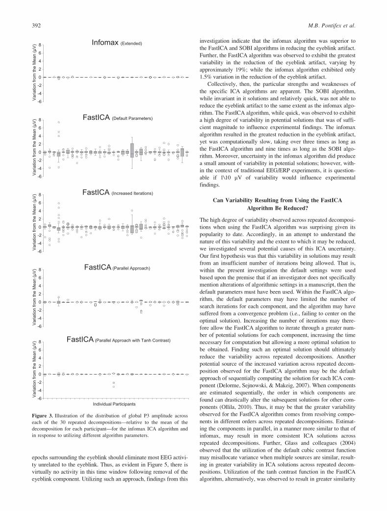
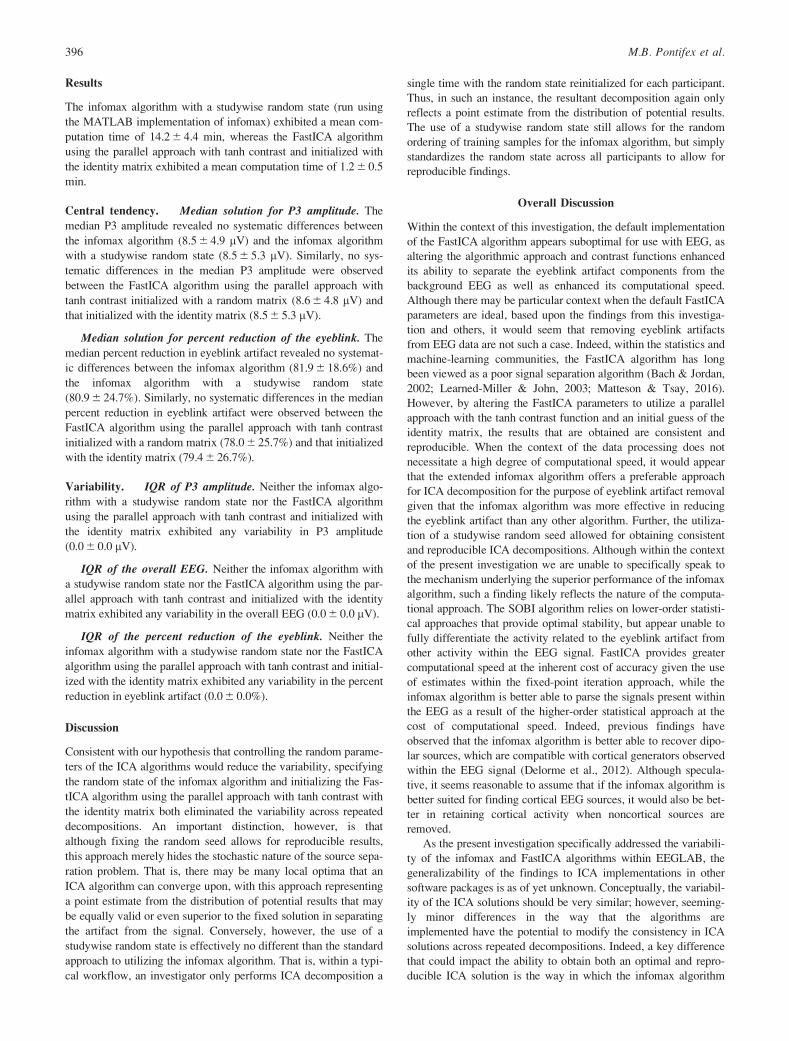
Figure 3. Illustration of the distribution of global P3 amplitude across

each of the 30 repeated decompositions—relative to the mean of the

decomposition for each participant—for the infomax ICA algorithm and

in response to utilizing different algorithm parameters.

392 M.B. Pontifex et al.

of the EEG data to the infomax algorithm following removal of the

eyeblink component (Glass et al., 2004). Collectively then, the

default FastICA parameters may not be ideally tuned to the charac-

teristics of EEG data, which may have contributed to the manifesta-

tion of the increased variability across repeated decompositions

(Artoni et al., 2014). Accordingly, we specifically tested the extent

to which variability induced by the FastICA algorithm following

removal of the eyeblink component might be reduced by increasing

the number of iterations, using a parallel approach, and using the

tanh contrast function in association with the parallel approach.

Method

Procedure. Replicating the methodological approach used above,

the data were processed by repeating 30 independent decomposi-

tions of the FastICA algorithm. To ensure that the variability was

200 %

Interquartile Range of Reduction of

Eye Blink Artifact

20 µV

Interquartile Range of

Overall EEG

10 µV

Interquartile Range of

P3 Amplitude

SOBIDefault

Parameters

InfomaxExtended

InfomaxExtended

Study-WiseRandom State

Increased IterationsFastICA

FastICAParallel Approach

Parallel Approach with Tanh Contrast

FastICA

Parallel Approach with Tanh Contrastwith Identity Matrix

FastICA

DefaultParameters

FastICA

Figure 4. Illustration of the topographic distribution in variability for P3 amplitude, the overall EEG, and the reduction in the eyeblink artifact across

all participants as a function of three popular ICA algorithms and from utilizing different algorithm parameters.

ICA variability 393

not increased as a result of failing to converge upon an optimal

solution, this process was repeated by increasing the maximum

number of iterations from 1,000 to 3,000. This process was further

repeated using the parallel approach with a stability parameter

enabled, and again changing the contrast function to tanh using the

parallel approach with a stability parameter enabled. Exemplar

MATLAB EEGLAB code is provided in Figure 1. Following each

ICA computation, the eyeblink artifact component was identified

Range ofEye Blink Artifact Reduction

Range ofStimulus-Locked Potentials

SOBIDefault

Parameters

FP1-20

60

140-200 200

Ampl

itude

(µV)

Time (ms)

Raw DataSolutions

InfomaxExtended

FP1-20

60

140-200 200

Ampl

itude

(µV)

Time (ms)

Pz-5

150 1000

Ampl

itude

(µV)

Time (ms)

InfomaxExtended

Study-WiseRandom State

IncreasedIterations

FastICAFP1-20

60

140-200 200

Ampl

itude

(µV)

Time (ms)

Pz-5

150 1000

Ampl

itude

(µV)

Time (ms)

FastICAParallel

Approach

FP1-20

60

140-200 200

Ampl

itude

(µV)

Time (ms)

Pz-5

150 1000

Ampl

itude

(µV)

Time (ms)

ParallelApproach withTanh Contrast

FastICAFP1-20

60

140-200 200

Ampl

itude

(µV)

Time (ms)

Pz-5

150 1000

Ampl

itude

(µV)

Time (ms)

ParallelApproach withTanh Contrastwith Identity

Matrix

FastICA

DefaultParameters

FastICAFP1-20

60

140-200 200

Ampl

itude

(µV)

Time (ms)

Pz-5

150 1000

Ampl

itude

(µV)

Time (ms)

Pz-5

150 1000

Ampl

itude

(µV)

Time (ms)

Pz-5

150 1000

Ampl

itude

(µV)

Time (ms)

Pz-5

150 1000

Ampl

itude

(µV)

Time (ms)

FP1-20

60

140-200 200

Ampl

itude

(µV)

Time (ms)

FP1-20

60

140-200 200

Ampl

itude

(µV)

Time (ms)

Figure 5. Illustration of the variability for the stimulus-locked average and eyeblink artifact average waveforms across all participants as a function of

three popular ICA algorithms and from utilizing different algorithm parameters.

394 M.B. Pontifex et al.

using the icablinkmetrics function (Pontifex et al., 2016), verified

using the EyeCatch function (Bigdely-Shamlo et al., 2013), and

removed. All postprocessing and variability quantification

approaches following removal of the eyeblink artifact component

were identical to those used above.

Statistical analysis. The analytical strategy mirrored that detailed

above, with the median and interquartile range of P3 amplitude, the

overall EEG, and the percent reduction in the eyeblink artifact pro-

vided in Table 1.

Results

The default FastICA algorithm exhibited a mean computation time

of 3.7 6 1.6 min. Increasing the possible iterations of the FastICA

algorithm resulted in a mean computation time of 6.8 6 3.5 min.

The mean computation time was 1.2 6 0.7 min for the FastICA

algorithm using the parallel approach and 1.0 6 0.2 min for the

FastICA parallel approach using the tanh contrast.

Central tendency. Median solution for P3 amplitude. The

median P3 amplitude was observed to be attenuated for the Fas-

tICA parallel approach using tanh at frontal/central electrode sites

(mean: 7.1 6 5.0 mV), relative to other variants of the FastICA

algorithm (mean: 7.6 6 5.1 mV; see Figure 2).

Median solution for percent reduction of the eyeblink. The

median percent reduction in eyeblink artifact was observed to be

greater for the FastICA parallel approach using tanh

(78.0 6 21.7%), relative to other variants of the FastICA algorithm

(mean: 70.5 6 19.2%; see Figure 2).

Variability. IQR of P3 amplitude. The IQR of P3 amplitude

was observed to be greater for the default FastICA algorithm and

FastICA with increased iterations (mean: 0.60 6 0.54 mV), relative

to the FastICA parallel approach and the FastICA parallel approach

using tanh (mean: 0.10 6 0.11 mV; see Figure (3 and 4), and 5).

IQR of the overall EEG. The IQR of the overall EEG similar-

ly reflected greater variability for the default FastICA algorithm

and FastICA with increased iterations (mean: 2.00 6 1.31 mV), rel-

ative to the FastICA parallel approach and the FastICA parallel

approach using tanh (mean: 0.27 6 0.31 mV; see Figure 4).

IQR of the percent reduction of the eyeblink. The IQR of

the percent reduction in eyeblink artifact observed greater variabili-

ty for the default FastICA algorithm and FastICA with increased

iterations (mean: 18.83 6 16.20%), relative to the FastICA parallel

approach and the FastICA parallel approach using tanh (mean:

3.38 6 5.91%; see Figure 4 and 5).

Discussion

In contrast to our initial hypothesis that the variability observed

across repeated decompositions when using the FastICA was the

result of a failure of the algorithm to converge upon an optimal

solution, the findings reported herein suggest that a major contribu-

tor to this variability is the sequential approach for determining

each component. That is, the parallel implementations of the Fas-

tICA algorithm resulted in an approximately 80% reduction in the

variability observed for P3 amplitude, the overall EEG, and the per-

cent reduction in the eyeblink artifact relative to the default imple-

mentation of FastICA. Thus, resolving components in parallel

appears to result in more consistent ICA solutions across decompo-

sitions relative to the default implementation of FastICA. Although

not drastically different from the default cubic contrast function,

utilization of the tanh contrast function of the parallel FastICA

algorithm, as suggested by Glass and colleagues (2004), did result

in a small reduction in variability for P3 amplitude, the overall

EEG, and reduction of the eyeblink with the additional benefit of a

faster computation time. However, the tanh contrast function was

associated with a slightly smaller P3 amplitude across frontal and

central electrodes.

Can Variability Be Reduced by Controlling the Random

Parameters?

Although the variability was minimized by utilizing the FastICA

algorithm with the parallel approach and tanh contrast function,

perfectly consistent results were not observed across repeated

decompositions. One potential source of this remaining variability

in the FastICA algorithm is the default utilization of an initial guess

of the ICA weights by way of a randomly generated matrix. Thus,

on each decomposition iteration, the FastICA algorithm generates a

different initial starting point for computing the ICA weights. Such

a source of variability may also be involved in the variability

observed from utilization of the infomax algorithm, as upon initiali-

zation of the algorithm the data points used for training are ran-

domly reordered. Thus, on each decomposition iteration, the

infomax algorithm may converge upon a different local optima

solution resulting in the observed variability. Accordingly, we spe-

cifically tested the extent to which these random parameters con-

tributed to the observed variability across repeated decompositions.

Method

Procedure. Replicating the methodological approach used above,

the data were processed by repeating 30 independent decomposi-

tions. To determine how the variability related to the infomax algo-

rithm may result from differences in the random reordering of

training samples across repeated decompositions, the MATLAB

implementation of infomax (runica) was utilized with the parame-

ter to reset the random seed turned off (an option available in

EEGLAB version 13.5.4b or newer), allowing for initializing the

algorithm using a studywise random state. As such a parameter

was not available through the binary implementation of infomax

(binica), all other parameters of the MATLAB implementation of

infomax (runica) were set to be equivalent to those used in the

binary implementation of infomax (binica) with the block size heu-

ristic drawn from MNE-Python (Gramfort et al., 2013) to most

closely approximate the heuristic used in the binary implementa-

tion (see Figure 1). To determine how the variability related to the

FastICA algorithm may result from differences in the random allo-

cation of the initialization matrix, the FastICA algorithm using the

parallel approach with tanh contrast was initialized using the identi-

ty matrix as the initial guess for each repeated decomposition.

Exemplar MATLAB EEGLAB code is provided in Figure 1. All

pos processing and variability quantification approaches following

removal of the eyeblink artifact component were identical to those

used above.

Statistical analysis. The analytical strategy mirrored that detailed

above, with the median and IQR range of P3 amplitude, the overall

EEG, and the percent reduction in the eyeblink artifact provided in

Table 1.

ICA variability 395

Results

The infomax algorithm with a studywise random state (run using

the MATLAB implementation of infomax) exhibited a mean com-

putation time of 14.2 6 4.4 min, whereas the FastICA algorithm

using the parallel approach with tanh contrast and initialized with

the identity matrix exhibited a mean computation time of 1.2 6 0.5

min.

Central tendency. Median solution for P3 amplitude. The

median P3 amplitude revealed no systematic differences between

the infomax algorithm (8.5 6 4.9 mV) and the infomax algorithm

with a studywise random state (8.5 6 5.3 mV). Similarly, no sys-

tematic differences in the median P3 amplitude were observed

between the FastICA algorithm using the parallel approach with

tanh contrast initialized with a random matrix (8.6 6 4.8 mV) and

that initialized with the identity matrix (8.5 6 5.3 mV).

Median solution for percent reduction of the eyeblink. The

median percent reduction in eyeblink artifact revealed no systemat-

ic differences between the infomax algorithm (81.9 6 18.6%) and

the infomax algorithm with a studywise random state

(80.9 6 24.7%). Similarly, no systematic differences in the median

percent reduction in eyeblink artifact were observed between the

FastICA algorithm using the parallel approach with tanh contrast

initialized with a random matrix (78.0 6 25.7%) and that initialized

with the identity matrix (79.4 6 26.7%).

Variability. IQR of P3 amplitude. Neither the infomax algo-

rithm with a studywise random state nor the FastICA algorithm

using the parallel approach with tanh contrast and initialized with

the identity matrix exhibited any variability in P3 amplitude

(0.0 6 0.0 mV).

IQR of the overall EEG. Neither the infomax algorithm with

a studywise random state nor the FastICA algorithm using the par-

allel approach with tanh contrast and initialized with the identity

matrix exhibited any variability in the overall EEG (0.0 6 0.0 mV).

IQR of the percent reduction of the eyeblink. Neither the

infomax algorithm with a studywise random state nor the FastICA

algorithm using the parallel approach with tanh contrast and initial-

ized with the identity matrix exhibited any variability in the percent

reduction in eyeblink artifact (0.0 6 0.0%).

Discussion

Consistent with our hypothesis that controlling the random parame-

ters of the ICA algorithms would reduce the variability, specifying

the random state of the infomax algorithm and initializing the Fas-

tICA algorithm using the parallel approach with tanh contrast with

the identity matrix both eliminated the variability across repeated

decompositions. An important distinction, however, is that

although fixing the random seed allows for reproducible results,

this approach merely hides the stochastic nature of the source sepa-

ration problem. That is, there may be many local optima that an

ICA algorithm can converge upon, with this approach representing

a point estimate from the distribution of potential results that may

be equally valid or even superior to the fixed solution in separating

the artifact from the signal. Conversely, however, the use of a

studywise random state is effectively no different than the standard

approach to utilizing the infomax algorithm. That is, within a typi-

cal workflow, an investigator only performs ICA decomposition a

single time with the random state reinitialized for each participant.

Thus, in such an instance, the resultant decomposition again only

reflects a point estimate from the distribution of potential results.

The use of a studywise random state still allows for the random

ordering of training samples for the infomax algorithm, but simply

standardizes the random state across all participants to allow for

reproducible findings.

Overall Discussion

Within the context of this investigation, the default implementation

of the FastICA algorithm appears suboptimal for use with EEG, as

altering the algorithmic approach and contrast functions enhanced

its ability to separate the eyeblink artifact components from the

background EEG as well as enhanced its computational speed.

Although there may be particular context when the default FastICA

parameters are ideal, based upon the findings from this investiga-

tion and others, it would seem that removing eyeblink artifacts

from EEG data are not such a case. Indeed, within the statistics and

machine-learning communities, the FastICA algorithm has long

been viewed as a poor signal separation algorithm (Bach & Jordan,

2002; Learned-Miller & John, 2003; Matteson & Tsay, 2016).

However, by altering the FastICA parameters to utilize a parallel

approach with the tanh contrast function and an initial guess of the

identity matrix, the results that are obtained are consistent and

reproducible. When the context of the data processing does not

necessitate a high degree of computational speed, it would appear

that the extended infomax algorithm offers a preferable approach

for ICA decomposition for the purpose of eyeblink artifact removal

given that the infomax algorithm was more effective in reducing

the eyeblink artifact than any other algorithm. Further, the utiliza-

tion of a studywise random seed allowed for obtaining consistent

and reproducible ICA decompositions. Although within the context

of the present investigation we are unable to specifically speak to

the mechanism underlying the superior performance of the infomax

algorithm, such a finding likely reflects the nature of the computa-

tional approach. The SOBI algorithm relies on lower-order statisti-

cal approaches that provide optimal stability, but appear unable to

fully differentiate the activity related to the eyeblink artifact from

other activity within the EEG signal. FastICA provides greater

computational speed at the inherent cost of accuracy given the use

of estimates within the fixed-point iteration approach, while the

infomax algorithm is better able to parse the signals present within

the EEG as a result of the higher-order statistical approach at the

cost of computational speed. Indeed, previous findings have

observed that the infomax algorithm is better able to recover dipo-

lar sources, which are compatible with cortical generators observed

within the EEG signal (Delorme et al., 2012). Although specula-

tive, it seems reasonable to assume that if the infomax algorithm is

better suited for finding cortical EEG sources, it would also be bet-

ter in retaining cortical activity when noncortical sources are

removed.

As the present investigation specifically addressed the variabili-

ty of the infomax and FastICA algorithms within EEGLAB, the

generalizability of the findings to ICA implementations in other

software packages is as of yet unknown. Conceptually, the variabil-

ity of the ICA solutions should be very similar; however, seeming-

ly minor differences in the way that the algorithms are

implemented have the potential to modify the consistency in ICA

solutions across repeated decompositions. Indeed, a key difference

that could impact the ability to obtain both an optimal and repro-

ducible ICA solution is the way in which the infomax algorithm

396 M.B. Pontifex et al.

implementation approaches setting of the random state. If the

implementation does not allow access to specifying the random

seed—as is the case in the current binary implementation of the

infomax algorithm in EEGLAB (binica)—the ability to obtain

reproducible results is hindered. Alternatively, if the implementa-

tion relies upon a fixed seed, the algorithm would obtain consistent

and reproducible results at the potential cost of the algorithm con-

verging upon a local-optimal solution—impacting the ability of the

algorithm to obtain the true optimal solution (if such a solution

even exists within real EEG data). Depending upon the implemen-

tation of these algorithms, the default preferences for using a ran-

dom relative to a fixed seed may differ. The benefit of open source

data processing platforms, however, is that such differences

between software implementations can more easily be detected and

modified (as in the case of updates to the runica function in

EEGLAB version 13.5.4b or newer) to allow the investigator to

specify the parameters appropriate for their needs. Further, as the

integration between MATLAB and other software packages, such

as Python, continues to be enhanced, it will be increasingly possi-

ble to utilize newer ICA algorithms or superior ICA implementa-

tions made available in other programming languages.

It is also necessary to note that the efficacy of the ICA decom-

position is dependent upon adequate preprocessing of the data. As

low-frequency aspects of the EEG signal typically account for large

proportions of variance, the application of a high-pass filter can

improve the ICA decomposition by removing slow drifts and DC

components (Winkler, Debener, M€uller, & Tangermann, 2015;

Zakeri, Assecondi, Bagshaw, & Arvanitis, 2014). Similarly, includ-

ing electrode channels located near the eye can improve the ICA

decomposition for the purposes of artifact removal, as the electro-

des provide greater information for the ICA algorithm to separate

the artifact from the background EEG (Zakeri et al., 2014).

Collectively, the present investigation illustrates how three pop-

ular ICA algorithms vary in the consistency of their solutions

across repeated decompositions using real EEG data. While the

present investigation used an automated eyeblink component selec-

tion approach that could have impacted the resultant variability, the

benefit of such an approach is the consistent application of the

same standards for component identification across repeated

decompositions, relying on convergence between two very differ-

ent methodologies of eyeblink component selection (i.e., icablink-

metrics—relying on time domain information, and EyeCatch—

relying on spatial information). Any variation then ultimately

occurs as a result of the ICA decomposition, with the data follow-

ing each decomposition representing one possible outcome. The

external relevance of these findings is that, when ICA approaches

are utilized to reconstruct data without a particular artifact, it is

important to understand the potential for hidden variance to be

induced. Although the measures of central tendency indicated mini-

mal differences in P3 amplitude across the three ICA approaches

(as illustrated in Figure 2), these findings should be interpreted as

reflective of a lack of differences in the midpoint of the solutions

across repeated decompositions across the three ICA approaches.

Whereas the interquartile range reflects the magnitude of the varia-

tion in the reconstructed data observed within each single subject

across repeated decompositions, thus the P3 ERP component on

any particular decomposition would be expected to fall somewhere

within the IQR (as illustrated in Figure 3).

Although this investigation used only data recorded in response

to a visual cognitive task, speculatively such variability should be

observed regardless of the context surrounding the recording of the

EEG signal so long as eyeblink artifacts occur. Such speculation is

drawn from the consistency between those findings specifically

focused on the P3 ERP component and those findings assessing the

variability across all sampling points of the EEG. Thus, although

this investigation utilized the P3 ERP component as a test case,

these findings should similarly generalize to other ERP compo-

nents. An important caveat to the present findings is that they do

not speak to the accuracy of the reconstructed EEG signal follow-

ing removal of the eyeblink artifact. That is, as real EEG data were

used, we are unable to know what the “ground truth” activity was

during the eyeblink activity. Thus, these ICA algorithms may differ

not only with respect to the consistency of their solutions, but the

accuracy of the solutions as well. Further, research is thus neces-

sary to investigate the accuracy of these ICA algorithmic

approaches. However, the present findings speak to the need for

investigators developing new ICA-based approaches to be attentive

not only to the accuracy of their approach but to the potential

uncertainty inherent within their approach. As Artoni and col-

leagues (2014) have demonstrated, such variability can be of use

within signal space for differentiating more stable sources that like-

ly reflect signal from those more variable sources that likely reflect

noise. However, within the context of reconstructing the EEG sig-

nal when artifact components are removed, these findings highlight

the ramifications of ICA uncertainty as it has the potential to intro-

duce additional sources of variance within EEG/ERP measures.

Given the growing interest in the repeatability of psychophysiologi-

cal findings, investigators should be particularly aware of the rela-

tive strengths and limitations of the algorithm and parameters

utilized for ICA decomposition as it relates to the potential to intro-

duce such additional sources of variance within their data.

References

Artoni, F., Menicucci, D., Delorme, A., Makeig, S., & Micera, S. (2014).RELICA: A method for estimating the reliability of independent com-ponents. NeuroImage, 103, 391–400. doi: 10.1016/j.neuroimage.2014.09.010

Bach, F. R., & Jordan, M. I. (2002). Kernel independent component analy-sis. Journal of Machine Learning Research, 3, 1–48.

Bell, A. J., & Sejnowski, T. J. (1995). An information-maximizationapproach to blind separationand blind deconvolution. Neural Computa-tion, 7, 1129–1159. doi: 10.1162/neco.1995.7.6.1129

Belouchrani, A., Abed-Meraim, K., Cardoso, J. F., & Moulines, E. (1997).A blind source separation technique using second-order statistics. IEEETransactions on Signal Processing, 45, 434–444.

Bigdely-Shamlo, N., Kreutz-Delgado, K., Kothe, C., & Makeig, S. (2013).EyeCatch: Data-mining over half a million EEG independent compo-nents to construct a fully-automated eye-component detector. Annual

International Conference of the IEEE Engineering in Medicine andBiology Society (pp. 5845/5848). Piscataway, NJ: IEEE Service Center.doi: 10.1109/EMBC.2013.6610881

Chatrian, G. E., Lettich, E., & Nelson, P. L. (1985). Ten percent electrodesystem for topographic studies of spontaneous and evoked EEG activi-ty. American Journal of EEG Technology, 25, 83–92. doi: 10.1080/00029238.1985.11080163

Debener, S., Makeig, S., Delorme, A., & Engel, A. K. (2005). What is novelin the novelty oddball paradigm? Functional significance of the noveltyP3 event-related potential as revealed by independent component analy-sis. Cognitive Brain Research, 22, 309–321. doi: 10.1016/j.cogbrainres.2004.09.006

Delorme, A., & Makeig, S. (2004). EEGLAB: An open source toolbox foranalysis of single-trial EEG dynamics. Journal of NeuroscienceMethods, 134, 9–21. doi: 10.1016/j.jneumeth.2003.10.009

ICA variability 397

Delorme, A., Palmer, J., Onton, J., Oostenveld, R., & Makeig, S. (2012).Independent EEG sources are diplar. PLOS ONE, 7(2), e30135.

Delorme, A., Sejnowski, T., & Makeig, S. (2007). Enhanced detection of arti-facts in EEG data using higher-order statistics and independent compo-nent analysis. NeuroImage, 34, 1443–1449. doi: 10.1016/j.neuroimage.2006.11.004

Duann, J. R., Jung, T. P., Kuo, W. J., Yeh, S., Makeig, S., Hsieh, J. C., &Sejnowski, T. J. (2001). Measuring the variability of event-relatedBOLD signals. Third International Workshop on Independent Compo-nent Analysis and Signal Separation, (pp. 528–533). San Diego, CA.

Duann, J. R., Jung, T. P., Makeig, S., & Sejnowski, T. J. (2003). Consisten-cy of infomax ICA decomposition of functional brain imaging data. 4thInternational Symposium on Independent Component Analysis andBlind Signal Separation, (pp. 289–294). Nara, Japan.

Esposito, F., Formisano, E., Seifritz, E., Goebel, R., Morrone, R.,Tedeschi, G., & Di Salle, F. (2002). Spatial independent componentanalysis of functional MRI time-series: To what extent do resultsdepend on the algorithm used? Human Brain Mapping, 16, 146–157.doi: 10.1002/hbm.10034

Glass, K. A., Frishkoff, G. A., Frank, R. M., Davey, C., Dien, J., Malony,A. D., & Tucker, D. M. (2004). A framework for evaluating ICA meth-ods of artifact removal from multichannel EEG. In C. G. Puntonet, &A. Prieto (Eds.), Independent component analysis and blind signal sep-aration. (pp. 1033–1040). Berlin, Germany: Springer.

Gramfort, A., Luessi, M., Larson, E., Engemann, D. A., Strohmeier, D.,Brodbeck, C., . . . H€am€al€ainen, M. (2013). MEG and EEG data analysiswith MNE-Python. Frontiers in Neuroscience, 7(267), 1–13. doi:10.3389/fnins.2013.00267

Gratton, G., Coles, M. G., & Donchin, E. (1983). A new method for off-line removal of ocular artifact. Electroencephalography and ClinicalNeurophysiology, 55, 468–484. doi: 10.1016/0013-4694(83)90135-9

Groppe, D. M., Makeig, S., & Kutas, M. (2009). Identifying reliable inde-pendent components via split-half comparisons. NeuroImage, 45,1199–1211. doi: 10.1016/j.neuroimage.2008.12.038

Harmeling, S., Meinecke, F., & Muller, K.-R. (2004). Injecting noise foranalysing the stability of ICA components. Signal Processing, 84, 255–266. doi: 10.1016/j.sigpro.2003.10.009

Himberg, J., Hyv€arinen, A., & Esposito, F. (2004). Validating the independentcomponents of neuroimaging time series via clustering and visualization.NeuroImage, 22, 1214–1222. doi: 10.1016/j.neuroimage.2004.03.027

Hoffmann, S., & Falkenstein, M. (2008). Correction of eye blink artefactsin the EEG: A comparison of two prominent methods. PLOS ONE, 3,1–11. doi: 10.1371/journal.pone.0003004

Hyv€arinen, A. (1999). Fast and robust fixed-point algorithms for indepen-dent component analysis. IEEE Transactions on Neural Networks, 10,626–634. doi: 10.1109/72.761722

Hyv€arinen, A., & Oja, E. (2000). Independent component analysis: Algo-rithms and applications. Neural Networks, 13, 411–430. doi: 0.1016/S0893-6080(00)00026-5

Jung, T.-P., Makeig, S., Humphries, C., Lee, T., McKeown, M. J., Iragui,V., & Sejnowski, T. J. (2000). Removing electroencephalographic arti-facts by blind source separation. Psychophysiology, 37, 163–178. doi:10.1111/1469-8986.3720163

Jung, T.-P., Makeig, S., McKeown, M. J., Bell, A. J., Lee, T.-W., &Sejnowski, T. J. (2001). Imaging brain dynamics using independentcomponent analysis. Proceedings of the IEEE, 89(7), 1107–1122.

Kamp, S.-M., Murphy, A. R., & Donchin, E. (2013). The component struc-ture of event-related potentials in the P300 speller paradigm. IEEETransactions on Neural Systems and Rehabilitation Engineering, 21,897–907. doi: 10.1109/TNSRE.2013.2285398

Learned-Miller, E. G., & John, W. F., III. (2003). ICA using spacings esti-mates of entropy. Journal of Machine Learning Research, 4, 1271–1295.

Lee, T. W. (1998). Independent component analysis. In Independent com-ponent analysis: Theory and applications (pp. 27–66). New York, NY:Springer. doi: 10.1007/978-1-4757-2851-4_2

Lee, T. W., Girolami, M., & Sejnowski, T. J. (1999). Independent compo-nent analysis using an extended infomax algorithm for mixed subGaus-sian and superGaussian sources. Neural Computation, 11, 417–441.doi: 10.1162/089976699300016719

Makeig, S., Westerfield, M., Jung, T.-P., Enghoff, S., Townsend, J.,Courchesne, E., & Sejnowski, T. J. (2002). Dynamic brain sources ofvisual evoked responses. Science, 295, 690–694. doi: 10.1126/science.1066168

Matteson, D. S., & Tsay, R. S. (2016). Independent component analysis viadistance covariance. Journal of the American Statistical Association.Advance online publication. doi: 10.1080/01621459.2016.1150851

Meinecke, F., Ziehe, A., Kawanabe, M., & M€uller, K.-R. (2002). A resam-pling approach to estimate the stability of one-dimensional or multidi-mensional independent components. IEEE Transactions on BiomedicalEngineering, 49, 1514–1525. doi: 10.1109/TBME.2002.805480

Mognon, A., Jovicich, J., Bruzzone, L., & Buiatti, M. (2011). ADJUST:An automatic EEG artifact detector based on the joint use of spatial andtemporal features. Psychophysiology, 48, 229–240. doi: 10.1111/j.1469-8986.2010.01061.x

Ollila, E. (2010). The deflation-based FastICA estimator: Statistical analy-sis revisited. IEEE Transactions on Signal Processing, 58, 1527–1541.doi: 10.1109/TSP.2009.2036072

Peirce, J. W. (2009). Generating stimuli for neuroscience using PsychoPy.Frontiers in Neuroinformatics, 2, 10. doi: 10.3389/neuro.11.010.2008

Polich, J. (2007). Updating P300: An integrative theory of P3a and P3b. Clin-ical Neurophysiology, 118, 2128–2148. doi: 10.1016/j.clinph.2007.04.019

Pontifex, M. B., Miskovic, V., & Laszlo, S. (2016). Are you removing thecorrect eye blink artifact component? A multi-measure time-domainapproach to facilitate component selection and automation.

Pontifex, M. B., Parks, A. C., Henning, D. A., & Kamijo, K. (2015). Singlebouts of exercise selectively sustain attentional processes. Psychophysi-ology. 52, 618–625. doi: 10.1111/psyp.12395

Stone, J. V. (2002). Independent component analysis: An introduction.Trends in Cognitive Sciences, 6, 59–64. doi: 10.1016/S1364-6613(00)01813-1

Winkler, I., Debener, S., M€uller, K. R., & Tangermann, M. (2015). On theinfluence of high-pass filtering on ICA-based artifact reduction inEEG-ERP. 37th Annual International Conference of the IEEE Engi-neering in Medicine and Biology Society (pp. 4101–4105.).

Zakeri, Z., Assecondi, S., Bagshaw, A. P., & Arvanitis, T. N. (2014). Influ-ence of signal preprocessing on ICA-based EEG decomposition. In L.M. Roa Romero (Ed.), XIII Mediterranean Conference on Medical andBiological Engineering and Computing 2013 (pp. 734–737). London,UK: Springer International Publishing. doi: 10.1007/978-3-319-00846-2_182

(RECEIVED May 17, 2016; ACCEPTED November 15, 2016)

398 M.B. Pontifex et al.