van der Vaart: Time Series
235
TIME SERIES A.W. van der Vaart Vrije Universiteit Amsterdam
Transcript of van der Vaart: Time Series

8/13/2019 van der Vaart: Time Series
http://slidepdf.com/reader/full/van-der-vaart-time-series 1/235
TIME SERIESA.W. van der Vaart
Vrije Universiteit Amsterdam

8/13/2019 van der Vaart: Time Series
http://slidepdf.com/reader/full/van-der-vaart-time-series 2/235
PREFACE
These are lecture notes for the courses “Tijdreeksen”, “Time Series” and “FinancialTimeSeries”. The material is more than can be treated in a one-semester course. Seenext section for the exam requirements.
Parts marked by an asterisk “*” do not belong to the exam requirements.Exercises marked by a single asterisk “*” are either hard or to be considered of
secondary importance. Exercises marked by a double asterisk “**” are questions to which
I do not know the solution.
Amsterdam, 1995–2010 (revisions, extensions),
A.W. van der Vaart
8/13/2019 van der Vaart: Time Series
http://slidepdf.com/reader/full/van-der-vaart-time-series 3/235
OLD EXAM
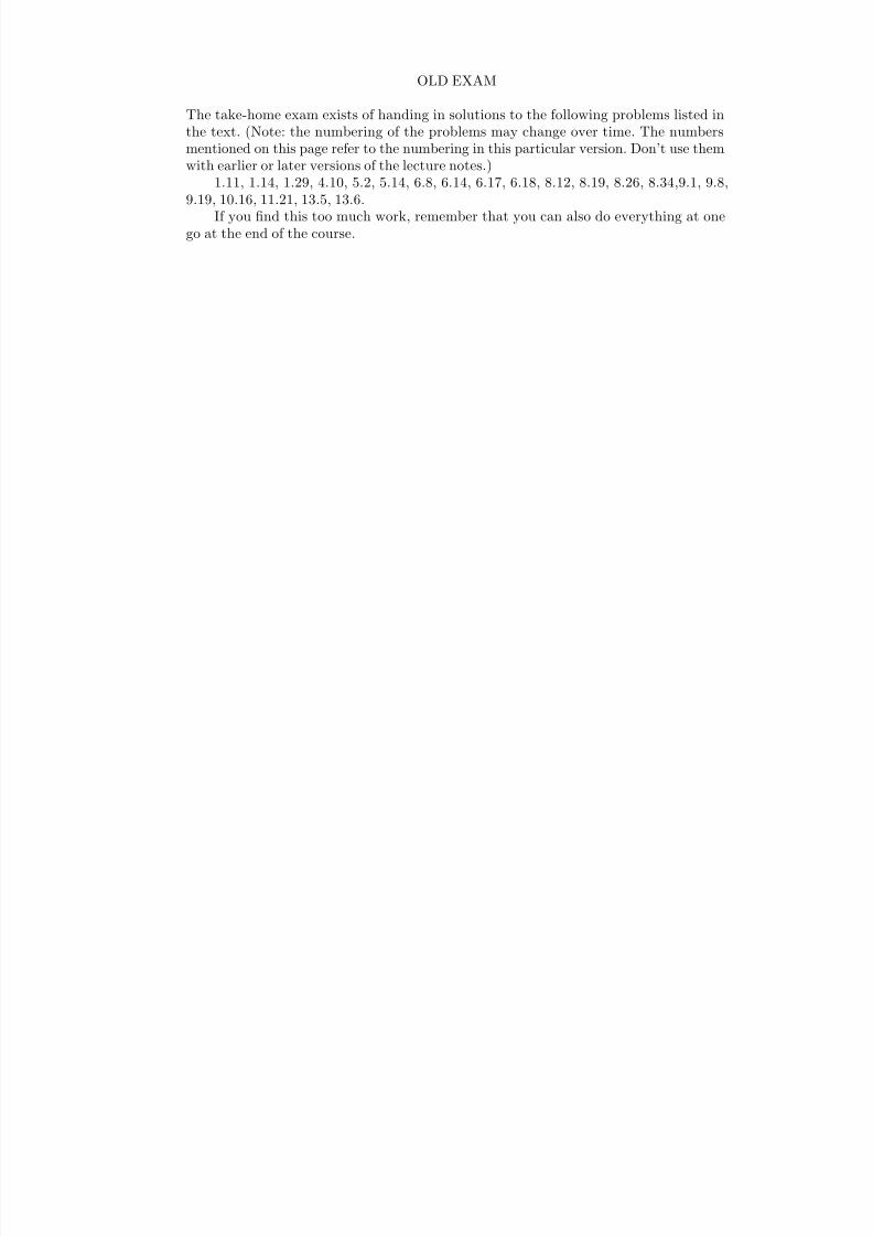
The take-home exam exists of handing in solutions to the following problems listed inthe text. (Note: the numbering of the problems may change over time. The numbersmentioned on this page refer to the numbering in this particular version. Don’t use themwith earlier or later versions of the lecture notes.)
1.11, 1.14, 1.29, 4.10, 5.2, 5.14, 6.8, 6.14, 6.17, 6.18, 8.12, 8.19, 8.26, 8.34,9.1, 9.8,9.19, 10.16, 11.21, 13.5, 13.6.
If you nd this too much work, remember that you can also do everything at onego at the end of the course.

8/13/2019 van der Vaart: Time Series
http://slidepdf.com/reader/full/van-der-vaart-time-series 4/235

8/13/2019 van der Vaart: Time Series
http://slidepdf.com/reader/full/van-der-vaart-time-series 5/235
[9] Gnedenko, B.V., (1962). Theory of Probability . Chelsea Publishing Company.[10] Hall, P. and Heyde, C.C., (1980). Martingale Limit Theory and Its Applications .
Academic Press, New York.[11] Hamilton, J.D., (1994). Time Series Analysis . Princeton.[12] Hannan, E.J. and Deistler, M., (1988). The Statistical Theory of Linear Systems .
John Wiley, New York.[13] Harvey, A.C., (1989). Forecasting, Structural Time Series Models and the Kalman
Filter . Cambridge University Press.[14] Mills, T.C., (1999). The Econometric Modelling of Financial Times Series . Cam-
bridge University Press.[15] Rio, A., (2000). Theorie Asymptotique des Processus Aleatoires Faiblement
Dependants . Springer Verlag, New York.[16] Rosenblatt, M., (2000). Gaussian and Non-Gaussian Linear Time Series and Ran-
dom Fields . Springer, New York.[17] Rudin, W., (1974). Real and Complex Analysis . McGraw-Hill.[18] Taniguchi, M. and Kakizawa, Y., (2000). Asymptotic Theory of Statistical Infer-
ence for Time Series . Springer.[19] van der Vaart, A.W., (1998). Asymptotic Statistics . Cambrdige University Press.

8/13/2019 van der Vaart: Time Series
http://slidepdf.com/reader/full/van-der-vaart-time-series 6/235
CONTENTS
1. Introduction . . . . . . . . . . . . . . . . . . . . . . . . . . . . . 21.1. Stationarity . . . . . . . . . . . . . . . . . . . . . . . . . . . 31.2. Transformations and Filters . . . . . . . . . . . . . . . . . . . . 121.3. Complex Random Variables . . . . . . . . . . . . . . . . . . . . 181.4. Multivariate Time Series . . . . . . . . . . . . . . . . . . . . . . 21
2. Hilbert Spaces and Prediction . . . . . . . . . . . . . . . . . . . . . 22
2.1. Hilbert Spaces and Projections . . . . . . . . . . . . . . . . . . . 222.2. Square-integrable Random Variables . . . . . . . . . . . . . . . . . 262.3. Linear Prediction . . . . . . . . . . . . . . . . . . . . . . . . . 292.4. Innovation Algorithm . . . . . . . . . . . . . . . . . . . . . . . 322.5. Nonlinear Prediction . . . . . . . . . . . . . . . . . . . . . . . 332.6. Partial Auto-Correlation . . . . . . . . . . . . . . . . . . . . . . 34
3. Stochastic Convergence . . . . . . . . . . . . . . . . . . . . . . . . 363.1. Basic theory . . . . . . . . . . . . . . . . . . . . . . . . . . . 363.2. Convergence of Moments . . . . . . . . . . . . . . . . . . . . . . 403.3. Arrays . . . . . . . . . . . . . . . . . . . . . . . . . . . . . . 413.4. Stochastic o and O symbols . . . . . . . . . . . . . . . . . . . . 423.5. Transforms . . . . . . . . . . . . . . . . . . . . . . . . . . . . 433.6. Cramer-Wold Device . . . . . . . . . . . . . . . . . . . . . . . 443.7. Delta-method . . . . . . . . . . . . . . . . . . . . . . . . . . 443.8. Lindeberg Central Limit Theorem . . . . . . . . . . . . . . . . . . 463.9. Minimum Contrast Estimators . . . . . . . . . . . . . . . . . . . 46
4. Central Limit Theorem . . . . . . . . . . . . . . . . . . . . . . . . 494.1. Finite Dependence . . . . . . . . . . . . . . . . . . . . . . . . 504.2. Linear Processes . . . . . . . . . . . . . . . . . . . . . . . . . 514.3. Strong Mixing . . . . . . . . . . . . . . . . . . . . . . . . . . 524.4. Uniform Mixing . . . . . . . . . . . . . . . . . . . . . . . . . 574.5. Martingale Differences . . . . . . . . . . . . . . . . . . . . . . . 584.6. Projections . . . . . . . . . . . . . . . . . . . . . . . . . . . . 614.7. Proof of Theorem 4.7 . . . . . . . . . . . . . . . . . . . . . . . 63
5. Nonparametric Estimation of Mean and Covariance . . . . . . . . . . . . 675.1. Mean . . . . . . . . . . . . . . . . . . . . . . . . . . . . . . 685.2. Auto Covariances . . . . . . . . . . . . . . . . . . . . . . . . . 725.3. Auto Correlations . . . . . . . . . . . . . . . . . . . . . . . . . 765.4. Partial Auto Correlations . . . . . . . . . . . . . . . . . . . . . 79
6. Spectral Theory . . . . . . . . . . . . . . . . . . . . . . . . . . . 826.1. Spectral Measures . . . . . . . . . . . . . . . . . . . . . . . . . 836.2. Aliasing . . . . . . . . . . . . . . . . . . . . . . . . . . . . . 916.3. Nonsummable lters . . . . . . . . . . . . . . . . . . . . . . . . 926.4. Spectral Decomposition . . . . . . . . . . . . . . . . . . . . . . 936.5. Multivariate Spectra . . . . . . . . . . . . . . . . . . . . . . 1006.6. Prediction in the Frequency Domain . . . . . . . . . . . . . . . . 103
7. Law of Large Numbers . . . . . . . . . . . . . . . . . . . . . . . 104

8/13/2019 van der Vaart: Time Series
http://slidepdf.com/reader/full/van-der-vaart-time-series 7/235

8/13/2019 van der Vaart: Time Series
http://slidepdf.com/reader/full/van-der-vaart-time-series 8/235
1Introduction
Oddly enough, a statistical time series is a mathematical sequence, not a series. In thisbook we understand a time series to be a doubly innite sequence
. . . , X −2 , X −1 , X 0 , X 1 , X 2 , . . .
of random variables or random vectors. We refer to the index t of X t as time and thinkof X t as the state or output of a stochastic system at time t. The interpretation of theindex as “time” is unimportant for the mathematical theory, which is concerned withthe joint distribution of the variables only, but the implied ordering of the variables isusually essential. Unless stated otherwise, the variable X t is assumed to be real valued,but we shall also consider sequences of random vectors, which sometimes have values inthe complex numbers. We often write “the time series X t ” rather than use the correct(X t : t Z ), and instead of “time series” we also speak of “process”, “stochastic process”,or “signal”.
We shall be interested in the joint distribution of the variables X t . The easiest way toensure that these variables, and other variables that we may introduce, possess joint laws,is to assume that they are dened as measurable maps on a single underlying probabilityspace. This is what we meant, but did not say in the preceding denition. Also in generalwe make the underlying probability space formal only if otherwise confusion might arise,and then denote it by (Ω , U , P), with ω denoting a typical element of Ω.
Time series theory is a mixture of probabilistic and statistical concepts. The proba-bilistic part is to study and characterize probability distributions of sets of variables X tthat will typically be dependent. The statistical problem is to determine the probabilitydistribution of the time series given observations X 1 , . . . , X n at times 1 , 2, . . . , n . Theresulting stochastic model can be used in two ways:
- understanding the stochastic system;- predicting the “future”, i.e. X n +1 , X n +2 , . . . ,.
8/13/2019 van der Vaart: Time Series
http://slidepdf.com/reader/full/van-der-vaart-time-series 9/235
1.1: Stationarity 3
1.1 StationarityIn order to have any chance of success at these tasks it is necessary to assume some a-priori structure of the time series. Indeed, if the X t could be completely arbitrary randomvariables, then ( X 1 , . . . , X n ) would constitute a single observation from a completelyunknown distribution on R n . Conclusions about this distribution would be impossible,let alone about the distribution of the future values X n +1 , X n +2 , . . ..
A basic type of structure is stationarity. This comes in two forms.
1.1 Denition. The time series X t is strictly stationary if the distribution (on R h +1 )of the vector (X t , X t +1 , . . . , X t + h ) is independent of t, for every h N .
1.2 Denition. The time series X t is stationary (or more precisely second order sta-tionary ) if EX t and EX t + h X t exist and are nite and do not depend on t, for every h N .
It is clear that a strictly stationary time series with nite second moments is alsostationary. For a stationary time series the auto-covariance and auto-correlation at lag h Z are dened by
γ X (h) = cov( X t + h , X t ),
ρX (h) = ρ(X t + h , X t ) = γ X (h)γ X (0)
.
The auto-covariance and auto-correlation are functions γ X : Z →R and ρX : Z → [−1, 1].Both functions are symmetric about 0. Together with the mean µ = E X t , they determinethe rst and second moments of the stationary time series. Much of time series (toomuch?) concerns this “second order structure”.
The autocovariance and autocorrelations functions are measures of (linear) de-pendence between the variables at different time instants, except at lag 0, whereγ X (0) = var X t gives the variance of (any) X t , and ρX (0) = 1.
1.3 Example (White noise) . A doubly innite sequence of independent, identicallydistributed random variables X t is a strictly stationary time series. Its auto-covariancefunction is, with σ2 = var X t ,
γ X (h) = σ2 , if h = 0,
0, if h = 0.Any stationary time series X t with mean zero and covariance function of this type iscalled a white noise series. Thus any mean-zero i.i.d. sequence with nite variances is awhite noise series. The converse is not true: there exist white noise series’ that are notstrictly stationary.
The name “noise” should be intuitively clear. We shall see why it is called “white”when discussing spectral theory of time series’ in Chapter 6.
White noise series’ are important building blocks to construct other series’, but fromthe point of view of time series analysis they are not so interesting. More interesting areseries of dependent random variables, so that, to a certain extent, the future can bepredicted from the past.

8/13/2019 van der Vaart: Time Series
http://slidepdf.com/reader/full/van-der-vaart-time-series 10/235
4 1: Introduction
0 50 100 150 200 250
- 2
- 1
0
1
2
Figure 1.1. Realization of a Gaussian white noise series of length 250.
1.4 EXERCISE. Construct a white noise sequence that is not strictly stationary.
1.5 Example (Deterministic trigonometric series) . Let A and B be given, uncorre-lated random variables with mean zero and variance σ2 , and let λ be a given number.Then
X t = A cos(tλ ) + B sin(tλ )
denes a stationary time series. Indeed, E X t = 0 and
γ X (h) = cov( X t + h , X t )= cos (t + h)λ cos(tλ ) var A + sin (t + h)λ sin(tλ ) var B
= σ2 cos(hλ ).
Even though A and B are random variables, this type of time series is called deterministic in time series theory. Once A and B have been determined (at time −∞say), the processbehaves as a deterministic trigonometric function. This type of time series is an importantbuilding block to model cyclic events in a system, but it is not the typical example of astatistical time series that we study in this course. Predicting the future is too easy inthis case.
8/13/2019 van der Vaart: Time Series
http://slidepdf.com/reader/full/van-der-vaart-time-series 11/235
1.1: Stationarity 5
1.6 Example (Moving average) . Given a white noise series Z t with variance σ2 anda number θ set
X t = Z t + θZ t−1 .
This is called a moving average of order 1. The series is stationary with E X t = 0 and
γ X (h) = cov( Z t + h + θZ t + h−1 , Z t + θZ t−1) =
(1 + θ2)σ2 , if h = 0,
θσ2
, if h = ±1,0, otherwise.
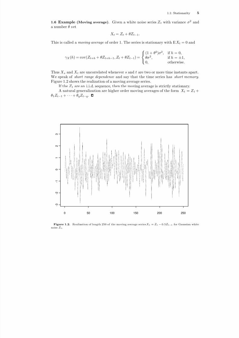
Thus X s and X t are uncorrelated whenever s and t are two or more time instants apart.We speak of short range dependence and say that the time series has short memory .Figure 1.2 shows the realization of a moving average series.
If the Z t are an i.i.d. sequence, then the moving average is strictly stationary.A natural generalization are higher order moving averages of the form X t = Z t +
θ1 Z t−1 + · · ·+ θqZ t−q .
0 50 100 150 200 250
- 3
- 2
- 1
0
1
2
3
Figure 1.2. Realization of length 250 of the moving average series X t = Z t − 0.5Z t − 1 for Gaussian whitenoise Z t .
8/13/2019 van der Vaart: Time Series
http://slidepdf.com/reader/full/van-der-vaart-time-series 12/235
6 1: Introduction
1.7 EXERCISE. Prove that the series X t in Example 1.6 is strictly stationary if Z t is astrictly stationary sequence.
1.8 Example (Autoregression) . Given a white noise series Z t with variance σ2 and anumber θ consider the equations
X t = θX t−1 + Z t , t Z .
To give this equation a clear meaning, we take the white noise series Z t as being denedon some probability space (Ω , U , P), and we look for a solution X t to the equation: atime series dened on the same probability space that solves the equation “pointwise inω” (at least for almost every ω).
This equation does not dene X t , but in general has many solutions. Indeed, wecan dene the sequence Z t and the variable X 0 in some arbitrary way on the givenprobability space and next dene the remaining variables X t for t Z \ 0 by theequation (if θ = 0). However, suppose that we are only interested in stationary solutions.Then there is either no solution or a unique solution, depending on the value of θ, as weshall now prove.
Suppose rst that |θ| < 1. By iteration we nd that
X t = θ(θX t−2 + Z t−1) + Z t = · · ·= θk X t−k + θk−1 Z t−k+1 + · · ·+ θZ t−1 + Z t .
For a stationary sequence X t we have that E( θk X t−k )2 = θ2k EX 20 → 0 as k → ∞. Thissuggests that a solution of the equation is given by the innite series
X t = Z t + θZ t−1 + θ2 Z t−2 + · · · =∞
j =0
θj Z t−j .
We show below in Lemma 1.28 that the series on the right side converges almost surely,so that the preceding display indeed denes some random variable X t . This is a movingaverage of innite order. We can check directly, by substitution in the equation, that X tsatises the auto-regressive relation. (For every ω for which the series converges; henceonly almost surely. We consider this to be good enough.)
If we are allowed to change expectations and innite sums, then we see that
EX t =∞
j =0
θj EZ t−j = 0,
γ X (h) =∞
i=0
∞
j =0
θi θj EZ t + h−i Z t−j =∞
j =0
θh + j θj σ2 1h + j ≥0 = θ|h |1 −θ2 σ2 .
We prove the validity of these formulas in Lemma 1.28. It follows that X t is indeeda stationary time series. In this example γ X (h) = 0 for every h, so that every pair of variables X s and X t are dependent. However, because γ X (h) → 0 at exponential speed

8/13/2019 van der Vaart: Time Series
http://slidepdf.com/reader/full/van-der-vaart-time-series 13/235
1.1: Stationarity 7
as h → ∞, this series is still considered to be short-range dependent. Note that γ X (h)oscillates if θ < 0 and decreases monotonely if θ > 0.
For θ = 1 the situation is very different: no stationary solution exists. To see thisnote that the equation obtained before by iteration now takes the form, for k = t,
X t = X 0 + Z 1 + · · ·+ Z t .
This implies that var( X t −X 0) = tσ 2 → ∞as t → ∞. However, by the triangle inequalitywe have that
sd(X t −X 0) ≤ sd X t + sd X 0 = 2 sd X 0 ,for a stationary sequence X t . Hence no stationary solution exists. The situation for θ = 1is explosive : the randomness increases signicantly as t → ∞ due to the introduction of a new Z t for every t. Figure 1.3 illustrates the nonstationarity of a random walk.
The cases θ = −1 and |θ| > 1 are left as exercises.The auto-regressive time series of order one generalizes naturally to auto-regressive
series of the form X t = φ1 X t−1 + · · ·φ pX t− p + Z t . The existence of stationary solutionsX t to this equation depends on the locations of the roots of the polynomial z → 1 −φ1z −φ2 z2 −· · ·−φ pz p, as is discussed in Chapter 8.
1.9 EXERCISE. Consider the cases θ = −1 and |θ| > 1. Show that in the rst case thereis no stationary solution and in the second case there is a unique stationary solution.[For
|θ
| > 1 mimic the argument for
|θ
| < 1, but with time reversed: iterate X
t−1 =
(1/θ )X t −Z t /θ .]
1.10 Example (GARCH) . A time series X t is called a GARCH(1, 1) process if, forgiven nonnegative constants α , θ and φ, and a given i.i.d. sequence Z t with mean zeroand unit variance, it satises the system of equations
X t = σt Z t ,
σ2t = α + φσ2
t−1 + θX 2t−1 .
The variable σt is interpreted as the scale or volatility of the time series X t at time t. Bythe second equation this is modelled as dependent on the “past”. To make this structureexplicit it is often included (or thought to be automatic) in the denition of a GARCH
process that, for every t ,(i) σt is a measurable function of X t−1 , X t−2 , . . .;(ii) Z t is independent of X t−1 , X t−2 , . . ..In view of the rst GARCH equation, properties (i)-(ii) imply that
EX t = E σt EZ t = 0,EX s X t = E( X s σt )EZ t = 0, (s < t ).
Therefore, a GARCH process with the extra properties (i)-(ii) is a white noise process.Furthermore,
E( X t |X t−1 , X t−2 , . . .) = σt EZ t = 0,E( X 2t |X t−1 , X t−2 , . . .) = σ2
t EZ 2t = σ2t .

8/13/2019 van der Vaart: Time Series
http://slidepdf.com/reader/full/van-der-vaart-time-series 14/235
8 1: Introduction
0 50 100 150 200 250
- 1 0
- 5
0
5
Figure 1.3. Realization of a random walk X t = Z t + ·· · + Z 0 of length 250 for Z t Gaussian white noise.
The rst equation shows that X t is a “martingale difference series”: the past does nothelp to predict future values of the time series. The second equation exhibits σ2
t as theconditional variance of X t given the past. Because σ2
t is a nontrivial time series by thesecond GARCH equation (if θ + φ = 0), the time series X t is not an i.i.d. sequence.
Because the conditional mean of X t given the past is zero, a GARCH process willuctuate around the value 0. A large deviation |X t−1| from 0 at time t−1 will cause a largeconditional variance σ2
t = α + θX 2t−1 + φσ2t−1 at time t , and then the deviation of X t =
σt Z t from 0 will tend to be large as well. Similarly, small deviations from 0 will tend to befollowed by other small deviations. Thus a GARCH process will alternate between periodsof big uctuations and periods of small uctuations. This is also expressed by sayingthat a GARCH process exhibits volatility clustering . Volatility clustering is commonlyobserved in time series of stock returns. The GARCH(1 , 1) process has become a popularmodel for such time series. Figure 1.5 shows a realization. The signs of the X t are equalto the signs of the Z t and hence will be independent over time.
The abbreviation GARCH is for “generalized auto-regressive conditional het-eroscedasticity”: the conditional variances are not i.i.d., and depend on the past throughan auto-regressive scheme. Typically, the conditional variances σ2
t are not directly ob-served, but must be inferred from the observed sequence X t .
Being a white noise process, a GARCH process can itself be used as input in an-
8/13/2019 van der Vaart: Time Series
http://slidepdf.com/reader/full/van-der-vaart-time-series 15/235
1.1: Stationarity 9
0 50 100 150 200 250
- 4
- 2
0
2
4
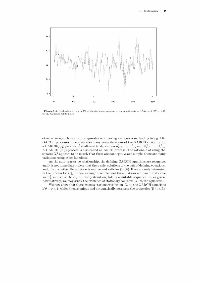
Figure 1.4. Realization of length 250 of the stationary solution to the equation X t = 0 .5X t − 1 +0 .2X t − 2 + Z tfor Z t Gaussian white noise.
other scheme, such as an auto-regressive or a moving average series, leading to e.g. AR-GARCH processes. There are also many generalizations of the GARCH structure. Ina GARCH( p, q ) process σ2
t is allowed to depend on σ2
t−1, . . . , σ2
t− p and X 2
t−1, . . . , X 2
t−q.
A GARCH (0 , q ) process is also called an ARCH process. The rationale of using thesquares X 2t appears to be mostly that these are nonnegative and simple; there are manyvariations using other functions.
As the auto-regressive relationship, the dening GARCH equations are recursive,and it is not immediately clear that there exist solutions to the pair of dening equations,and, if so, whether the solution is unique and satises (i)-(ii). If we are only interestedin the process for t ≥ 0, then we might complement the equations with an initial valuefor σ2
0 , and solve the equations by iteration, taking a suitable sequence Z t as given.Alternatively, we may study the existence of stationary solutions X t to the equations.
We now show that there exists a stationary solution X t to the GARCH equationsif θ + φ < 1, which then is unique and automatically possesses the properties (i)-(ii). By

8/13/2019 van der Vaart: Time Series
http://slidepdf.com/reader/full/van-der-vaart-time-series 16/235
10 1: Introduction
iterating the GARCH relation we nd that, for every n ≥0,
σ2t = α + ( φ + θZ 2t−1)σ2
t−1 = α + αn
j =1
(φ + θZ 2t−1) ×· · ·×(φ + θZ 2t−j )
+ ( φ + θZ 2t−1) ×· · ·×(φ + θZ 2t−n −1)σ2t−n −1 .
The sequence (φ+ θZ 2t−1) · · ·(φ+ θZ 2t−n −1) ∞n =1 , which consists of nonnegative variables
with means ( φ + θ)n +1
, converges in probability to zero if θ + φ < 1. If the time seriesσ2t is bounded in probability as t → ∞, then the term on the far right converges to zero
in probability as n → ∞. Thus for a stationary solution ( X t , σt ) we must have
(1.1) σ2t = α + α
∞
j =1(φ + θZ 2t−1) · · ·(φ + θZ 2t−j ).
This series has positive terms, and hence is always well dened. It is easily checked thatthe series converges in mean if and only if θ + φ < 1 (cf. Lemma 1.26). Given an i.i.d.series Z t , we can then dene a process X t by rst dening the conditional variances σ2
t by(1.1), and next setting X t = σt Z t . It can be veried by substitution that this process X tsolves the GARCH relationship. Hence a stationary solution to the GARCH equationsexists if φ + θ < 1.
Because Z t is independent of Z t−1 , Z t−2 , . . ., by (1.1) it is also independent of σ2
t−1 , σ2t−2 , . . ., and hence also of X t−1 = σt−1Z t−1 , X t−2 = σt−2Z t−2 , . . .. In addition
it follows that the time series X t = σt Z t is strictly stationary, being a xed measurabletransformation of ( Z t , Z t−1 , . . .) for every t.
By iterating the auto-regressive relation σ2t = φσ2
t−1 + W t , with W t = α + θX 2t−1 ,in the same way as in Example 1.8, we also nd that for the stationary solution σ2
t =∞j =0 φj W t−j . Hence σt is σ(X t−1 , X t−2 , . . .)-measurable.
An inspection of the preceding argument shows that a strictly stationary solutionexists under a weaker condition than φ + θ < 1. This is because the innite series (1.1)may converge almost surely, without converging in mean (see Exercise 1.14). We shallstudy this further in Chapter 9.
1.11 EXERCISE. Let θ + φ
[0, 1) and 1
−κθ2
−φ2
−2θφ > 0, where κ = E Z 4t . Show
that the second and fourth (marginal) moments of a stationary GARCH process aregiven by α/ (1 −θ −φ) and κα 2(1 + θ + φ)/ (1 −κθ2 −φ2 −2θφ)(1 −θ −φ). From thiscompute the kurtosis of the GARCH process with standard normal Z t . [You can use(1.1), but it is easier to use the GARCH relations.]
1.12 EXERCISE. Show that E X 4t = ∞ if 1−κθ2 −φ2 −2θφ = 0.
1.13 EXERCISE. Suppose that the process X t is square-integrable and satises theGARCH relation for an i.i.d. sequence Z t such that Z t is independent of X t−1 , X t−2 , . . .and such that σ2
t = E( X 2t |X t−1 , X t−2 , . . .), for every t , and some α,φ,θ > 0. Show thatφ + θ < 1. [Derive that E X 2t = α + α n
j =1 (φ + θ)j + ( φ + θ)n +1 EX 2t−n −1 .]

8/13/2019 van der Vaart: Time Series
http://slidepdf.com/reader/full/van-der-vaart-time-series 17/235
1.1: Stationarity 11
0 100 200 300 400 500
- 5
0
5
Figure 1.5. Realization of the GARCH(1 , 1) process with α = 0 .1, φ = 0 and θ = 0 .8 of length 500 for Z tGaussian white noise.
1.14 EXERCISE. Let Z t be an i.i.d. sequence with E log( Z 2t ) < 0. Show that∞j =0 Z 2t Z 2t−1 · · ·Z 2t−j < ∞ almost surely. [Use the Law of Large Numbers.]
1.15 Example (Stochastic volatility) . A general approach to obtain a time serieswith volatility clustering is to dene X t = σt Z t for an i.i.d. sequence Z t and a process σtthat depends “positively on its past”. A GARCH model ts this scheme, but a simpler
construction is to let σt depend only on its own past and independent noise. Because σtis to have an interpretation as a scale parameter, we restrain it to be positive. One wayto combine these requirements is to set
h t = θh t−1 + W t ,
σ2t = eh t ,
X t = σt Z t .
Here W t is a white noise sequence, ht is a (stationary) solution to the auto-regressiveequation, and the process Z t is i.i.d. and independent of the process W t . If θ > 0 andσt−1 = eh t − 1 / 2 is large, then σt = eh t / 2 will tend to be large as well. Hence the processX t will exhibit volatility clustering.

8/13/2019 van der Vaart: Time Series
http://slidepdf.com/reader/full/van-der-vaart-time-series 18/235
8/13/2019 van der Vaart: Time Series
http://slidepdf.com/reader/full/van-der-vaart-time-series 19/235
1.2: Transformations and Filters 13
0 50 100 150 200 250
- 1 0
- 5
0
5
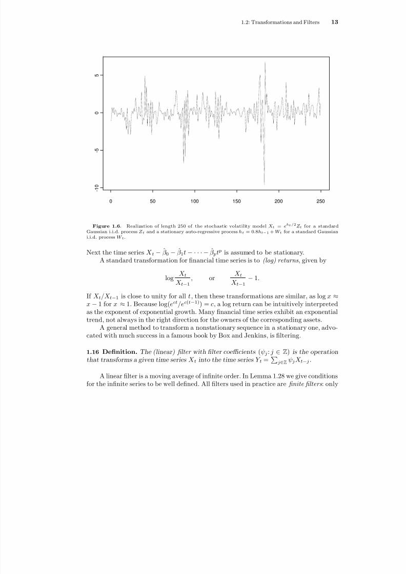
Figure 1.6. Realization of length 250 of the stochastic volatility model X t = eh t / 2 Z t for a standardGaussian i.i.d. process Z t and a stationary auto-regressive process h t = 0 .8h t − 1 + W t for a standard Gaussiani.i.d. process W t .
Next the time series X t − β 0 − β 1 t −· · ·− β pt p is assumed to be stationary.A standard transformation for nancial time series is to (log) returns , given by
log X tX t−1
, or X t
X t−1 −1.
If X t /X t
−1 is close to unity for all t , then these transformations are similar, as log x
≈x −1 for x ≈ 1. Because log(ect /e c( t−1) ) = c, a log return can be intuitively interpretedas the exponent of exponential growth. Many nancial time series exhibit an exponentialtrend, not always in the right direction for the owners of the corresponding assets.
A general method to transform a nonstationary sequence in a stationary one, advo-cated with much success in a famous book by Box and Jenkins, is ltering.
1.16 Denition. The (linear) lter with lter coefficients (ψj : j Z ) is the operationthat transforms a given time series X t into the time series Y t = j Z ψj X t−j .
A linear lter is a moving average of innite order. In Lemma 1.28 we give conditionsfor the innite series to be well dened. All lters used in practice are nite lters : only
8/13/2019 van der Vaart: Time Series
http://slidepdf.com/reader/full/van-der-vaart-time-series 20/235
14 1: Introduction
1984 1986 1988 1990 1992
1 . 0
1 . 5
2 . 0
2 . 5
1984 1986 1988 1990 1992
- 0 . 2
- 0 . 1
0 . 0
0 . 1
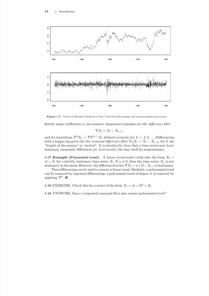
Figure 1.7. Prices of Hewlett Packard on New York Stock Exchange and corresponding log returns.
nitely many coefficients ψj are nonzero. Important examples are the difference lter
X t = X t −X t−1 ,
and its repetitions k X t = k−1 X t dened recursely for k = 2, 3, . . .. Differencingwith a bigger lag gives the the seasonal difference lter k X t = X t −X t−k , for k the“length of the season” or “period”. It is intuitively clear that a time series may havestationary (seasonal) differences (or increments ), but may itself be nonstationary.
1.17 Example (Polynomial trend) . A linear trend model could take the form X t =at + Z t for a strictly stationary time series Z t . If a = 0, then the time series X t is notstationary in the mean. However, the differenced series X t = a + Z t −Z t−1 is stationary.
Thus differencing can be used to remove a linear trend. Similarly, a polynomial trendcan be removed by repeated differencing: a polynomial trend of degree k is removed byapplying k .
1.18 EXERCISE. Check this for a series of the form X t = at + bt2 + Z t .
1.19 EXERCISE. Does a (repeated) seasonal lter also remove polynomial trend?

8/13/2019 van der Vaart: Time Series
http://slidepdf.com/reader/full/van-der-vaart-time-series 21/235
1.2: Transformations and Filters 15
0 20 40 60 80 100
0
2 0 0
4 0 0
6 0 0
0 20 40 60 80 100
0
2
4
6
8
1 0
0 20 40 60 80 100
- 4
- 2
0
2
4
Figure 1.8. Realization of the time series t + 0 .05 t 2 + X t for the stationary auto-regressive process X tsatisfying X t −0.8X t − 1 = Z t for Gaussian white noise Z t , and the same series after once and twice differencing.
1.20 Example (Random walk) . A random walk is dened as the sequence of partialsums X t = Z 1 + Z 2 + · · ·+ Z t of an i.i.d. sequence Z t (with X 0 = 0). A random walk isnot stationary, but the differenced series X t = Z t certainly is.
1.21 Example (Monthly cycle) . If X t is the value of a system in month t, then 12 X tis the change in the system during the past year. For seasonable variables without trendthis series might be modelled as stationary. For series that contain both yearly seasonalityand polynomial trend, the series k 12 X t might be stationary.
1.22 Example (Weekly averages) . If X t is the value of a system at day t , then Y t =(1/ 7) 6
j =0 X t−j is the average value over the last week. This series might show trend,but should not show seasonality due to day-of-the-week. We could study seasonalityby considering the time series X t −Y t , which results from ltering the series X t withcoefficients (ψ0 , . . . , ψ6) = (6 / 7, −1/ 7, . . . , −1/ 7).
1.23 Example (Exponential smoothing) . An ad-hoc method for predicting the futureis to equate the future to the present or, more generally, to the average of the lastk observed values of a time series. When averaging past values it is natural to give

8/13/2019 van der Vaart: Time Series
http://slidepdf.com/reader/full/van-der-vaart-time-series 22/235
16 1: Introduction
more weight to the most recent values. Exponentially decreasing weights appear to havesome popularity. This corresponds to predicting a future value of a time series X t bythe weighted average ∞j =0 θj (1 −θ)−1X t−j for some θ (0, 1). The coefficients ψj =θj / (1 −θ) of this lter decrease exponentially and satisfy ψj = 1.
1.24 EXERCISE (Convolution) . Show that the result of two lters with coefficientsα j and β j applied in turn (if well dened) is the lter with coefficients γ j given byγ k =
j α j β k−j . This is called the convolution of the two lters. Infer that ltering is
commutative.1.25 Denition. A lter with coefficients ψj is causal if ψj = 0 for every j < 0.
For a causal lter the variable Y t = j ψj X t−j depends only on the valuesX t , X t−1 , . . . of the original time series in the present and past, not the future. This isimportant for prediction. Given X t up to some time t , we can calculate Y t up to time t .If Y t is stationary, we can use results for stationary time series to predict the future valueY t +1 . Next we predict the future value X t +1 by X t +1 = ψ−1
0 (Y t +1 − j> 0 ψj X t +1 −j ).In order to derive conditions that guarantee that an innite lter is well dened, we
start with a lemma concerning series’ of random variables. Recall that a series t x t of nonnegative numbers is always well dened (although possibly ∞), where the order of summation is irrelevant. Furthermore, for general numbers x t the absolute convergence
t |xt
| <
∞ implies that
t
xt exists as a nite number, where the order of summationis again irrelevant. We shall be concerned with series indexed by t belonging to somecountable set T , such as N , Z , or Z 2 . It follows from the preceding that t T x t is welldened as a limit as n → ∞ of partial sums t T n xt , for any increasing sequence of nite subsets T n T with union T , if either every xt is nonnegative or t |x t | < ∞.For instance, in the case that the index set T is equal to Z , we can choose the setsT n = t Z : |t| ≤ n.
1.26 Lemma. Let (X t : t T ) be an arbitrary countable set of random variables.(i) If X t ≥0 for every t , then E t X t = t EX t (possibly + ∞);
(ii) If t E|X t | < ∞, then the series t X t converges absolutely almost surely and E t X t = t EX t .
Proof. Suppose T =
j T j for an increasing sequence T 1
T 2
·· · of nite subsets of
T . Assertion (i) follows from the monotone convergence theorem applied to the variablesY j = t T j X t . For the proof of (ii) we rst note that Z = t |X t | is well dened, withnite mean E Z = t E|X t |, by (i). Thus t |X t | converges almost surely to a nite limit,and hence Y : = t X t converges almost surely as well. The variables Y j = t T j X t aredominated by Z and converge to Y as j ↑ ∞. Hence EY j → EY by the dominatedconvergence theorem.
The dominated convergence theorem in the proof of (ii) actually gives a better result,namely: if t E|X t | < ∞, then
Et T
X t −t T j
X t → 0, if T 1 T 2 ·· · ↑T.

8/13/2019 van der Vaart: Time Series
http://slidepdf.com/reader/full/van-der-vaart-time-series 23/235
1.2: Transformations and Filters 17
This is called the convergence in mean of the series t X t . The analogous convergenceof the second moment is called the convergence in second mean . Alternatively, we speakof “convergence in quadratic mean” or “convergence in L1 or L2”.
1.27 EXERCISE. Suppose that E |X n −X | p → 0 and E|X | p < ∞ for some p ≥1. Showthat E X kn → EX k for every 0 < k ≤ p.
1.28 Lemma. Let (Z t: t
Z ) be an arbitrary time series and let
j |ψ
j | <
∞.
(i) If sup t E|Z t | < ∞, then j ψj Z t−j converges absolutely, almost surely and in mean.(ii) If sup t E|Z t |2 < ∞, then j ψj Z t−j converges in second mean as well.
(iii) If the series Z t is stationary, then so is the series X t = j ψj Z t−j and γ X (h) =l j ψj ψj + l−h γ Z (l).
Proof. (i). Because t E|ψj Z t−j | ≤ supt E|Z t | j |ψj | < ∞, it follows by (ii) of thepreceding lemma that the series j ψj Z t is absolutely convergent, almost surely. Theconvergence in mean follows as in the remark following the lemma.
(ii). By (i) the series converges almost surely, and j ψj Z t−j − |j |≤k ψj Z t−j =
|j |>k ψj Z t−j . By the triangle inequality we have
|j |>kψj Z t−j
2
≤ |j |>k |ψj Z t−j |2
=|j |>k |i |>k |ψj ||ψi ||Z t−j ||Z t−i |.
By the Cauchy-Schwarz inequality E |Z t−j ||Z t−i | ≤ E|Z t−j |2|EZ t−i |21/ 2 , which is
bounded by sup t E|Z t |2 . Therefore, in view of (i) of the preceding lemma the expec-tation of the right side (and hence the left side) of the preceding display is boundedabove by
|j |>k |i |>k|ψj ||ψi |sup
tE|Z t |2 =
|j |>k|ψj |
2sup
tE|Z t |2 .
This converges to zero as k → ∞.(iii). By (i) the series
j ψj Z t−j converges in mean. Therefore, E j ψj Z t−j =
j ψj EZ t , which is independent of t. Using arguments as before, we see that we canalso justify the interchange of the order of expectations (hidden in the covariance) anddouble sums in
γ X (h) = covj
ψj Z t + h−j ,i
ψi Z t−i
=j i
ψj ψi cov(Z t + h −j , Z t−i ) =j i
ψj ψi γ Z (h − j + i).
This can be written in the form given by the lemma by the change of variables ( j, i ) →( j, j + l −h).

8/13/2019 van der Vaart: Time Series
http://slidepdf.com/reader/full/van-der-vaart-time-series 24/235
18 1: Introduction
1.29 EXERCISE. Suppose that the series Z t in (iii) is strictly stationary. Show that theseries X t is strictly stationary whenever it is well dened. [You need measure theory tomake the argument mathematically rigorous(?).]
* 1.30 EXERCISE. For a white noise series Z t , part (ii) of the preceding lemma can be im-proved: Suppose that Z t is a white noise sequence and j ψ
2j < ∞. Show that j ψj Z t−j
converges in second mean. [For this exercise you may want to use material from Chap-ter 2.]
1.3 Complex Random VariablesEven though no real-life time series is complex valued, the use of complex numbers isnotationally convenient to develop the mathematical theory. In this section we discusscomplex-valued random variables.
A complex random variable Z is a map from some probability space into the eldof complex numbers whose real and imaginary parts are random variables. For complexrandom variables Z = X + iY , Z 1 and Z 2 , we dene
EZ = E X + iEY,var Z = E |Z −EZ |2 ,
cov(Z 1 , Z 2) = E( Z 1 −EZ 1)(Z 2 −EZ 2).
Here the overbar means complex conjugation . Some simple properties are, for α, β C ,
EαZ = αEZ, EZ = E Z,
var Z = E |Z |2 − |EZ |2 = var X + var Y = cov( Z, Z ),
var( αZ ) = |α |2 var Z,
cov(αZ 1 , βZ 2) = αβ cov(Z 1 , Z 2),
cov(Z 1 , Z 2) = cov( Z 2 , Z 1) = E Z 1Z 2 −EZ 1EZ 2 .
A complex random vector is of course a vector Z = ( Z 1 , . . . , Z n )T of complex randomvariables Z i dened on the same probability space. Its covariance matrix Cov( Z ) is the(n ×n) matrix of covariances cov( Z i , Z j ).
1.31 EXERCISE. Prove the preceding identities.
1.32 EXERCISE. Prove that a covariance matrix Σ = Cov( Z ) of a complex randomvector Z is Hermitian (i.e. Σ = Σ T ) and nonnegative-denite (i.e. αΣ α T ≥ 0 for everyα C n ). Here Σ T is the reection of a matrix, dened to have ( i, j )-element Σ j,i .
A complex time series is a (doubly innite) sequence of complex-valued randomvariables X t . The denitions of mean, covariance function, and (strict) stationarity given

8/13/2019 van der Vaart: Time Series
http://slidepdf.com/reader/full/van-der-vaart-time-series 25/235
1.3: Complex Random Variables 19
for real time series apply equally well to complex time series. In particular, the auto-covariance function of a stationary complex time series is the function γ X : Z →C denedby γ X (h) = cov( X t + h , X t ). Lemma 1.28 also extends to complex time series Z t , wherein (iii) we must read γ X (h) = l j ψj ψ j + l−h γ Z (l).
1.33 EXERCISE. Show that the auto-covariance function of a complex stationary timeseries X t is conjugate symmetric: γ X (−h) = γ X (h), for every h Z . (The positions of X t + h and X t in the denition γ X (h) = cov( X t + h , X t ) matter!)
Useful as these denitions are, it should be noted that the second-order structure of acomplex-valued time series is only partly described by its covariance function. A complexrandom variable is geometrically equivalent to the two-dimensional real vector of its realand imaginary parts. More generally, a complex random vector Z = ( Z 1 , . . . , Z n ) of dimension n can be identied with the 2 n-dimensional real vector that combines all realand imaginary parts. The second order structure of the latter vector is determined bya 2n-dimensional real covariance matrix, and this is not completely determined by the(n ×n) complex covariance matrix of Z . This is clear from comparing the dimensionsof these objects. For instance, for n = 1 the complex covariance matrix of Z is simplythe single positive number var Z , whereas the covariance matrix of its pair of real andimaginary parts is a symmetric (2 ×2)-matrix. This discrepancy increases with n. Thecovariance matrix of a complex vector of dimension n contains n reals on the diagonaland 12 n(n −1) complex numbers off the diagonal, giving n + n(n −1) = n2 reals in total,whereas a real covariance matrix of dimension 2 n varies over an open set of 1
2 2n(2n + 1)reals.
* 1.3.1 Complex Gaussian vectors
It is particularly important to keep this in mind when working with complex Gaussianvectors. A complex random vector Z = ( Z 1 , . . . , Z n ) is normally distributed or Gaussian if the 2n-vector of all its real and imaginary parts is multivariate-normally distributed.The latter distribution is determined by the mean vector and the covariance matrixof the latter 2 n-vector. The mean vector is one-to-one related to the (complex) meanvector of Z , but the complex covariances cov( Z i , Z j ) do not completely determine thecovariance matrix of the combined real and imaginary parts. This is sometimes resolvedby requiring that the covariance matrix of the 2 n-vector has the special form
(1.2) 12
Re Σ −Im ΣIm Σ Re Σ .
Here Re Σ and Im Σ are the real and imaginary parts of the complex covariance matrixΣ = Re Σ + i ImΣ of Z . A Gaussian distribution with covariance matrix of this typeis sometimes called circular complex normal . This distribution is completely describedby the mean vector µ and covariance matrix Σ, and can be referred to by a code suchas N n (µ, Σ). However, the additional requirement (1.2) imposes a relationship betweenthe vectors of real and imaginary parts of Z , which seems not natural for a generaldenition of a Gaussian complex vector. For instance, under the requirement (1.2) a

8/13/2019 van der Vaart: Time Series
http://slidepdf.com/reader/full/van-der-vaart-time-series 26/235
8/13/2019 van der Vaart: Time Series
http://slidepdf.com/reader/full/van-der-vaart-time-series 27/235
1.4: Multivariate Time Series 21
as (1.2). Show that the n-vector Z = X + iY possesses covariance matrix Σ. Also showthat E( Z −EZ )(Z −EZ )T = 0.
1.38 EXERCISE. Let Z and Z be independent complex random vectors with mean zeroand covariance matrix Σ.(i) Show that E(Re Z )(Re Z )T + E(Im Z )(Im Z )T = Re Σ and E(Im Z )(Re Z )T −E(Re Z )(Im Z )T = ImΣ.
(ii) Show that the 2 n-vector ( X T , Y T )T dened by X = (Re Z + Im Z )/ √ 2 and Y =
(−Re Z + Im Z )/ √ 2 possesses covariance matrix (1.2).(iii) Show that the 2 n-vector (Re Z T , Im Z T )T does not necessarily have this property.
1.39 EXERCISE. Say that a complex n-vector Z = X + iY is N n (µ, Σ) distributed if the2n real vector ( X T , Y T )T is multivariate normally distributed with mean (Re µ, Im µ)and covariance matrix (1.2). Show that:(i) If Z is N (µ, Σ)-distributed, then AZ + b is N (Aµ + b, AΣ AT )-distributed.
(ii) If Z 1 and Z 2 are independent and N (µi , Σ i )-distributed, then Z 1 + Z 2 is N (µ1 +µ2 , Σ 1 + Σ 2 )-distributed.
(iii) If X is a real vector and N (µ, Σ)-dstributed and A is a complex matrix, then AX is typically not complex normally distributed.
1.4 Multivariate Time SeriesIn many applications we are interested in the time evolution of several variables jointly.This can be modelled through vector-valued time series. The denition of a station-ary time series applies without changes to vector-valued series X t = ( X t, 1 , . . . , X t,d )T .Here the mean E X t is understood to be the vector (E X t, 1 , . . . , X t,d )T of means of thecoordinates and the auto-covariance function is dened to be the matrix
γ X (h) = cov(X t + h,i , X t,j )i,j =1 ,...,d
= E( X t + h −EX t + h )(X t −EX t )T .
The auto-correlation at lag h is dened as
ρX (h) = ρ(X t + h,i , X t,j )i,j =1 ,...,d
= diag γ X (0) γ X (h)diag γ X (0) .
The study of properties of multivariate time series can often be reduced to the study of univariate time series by taking linear combinations α T X t of the coordinates. The rstand second moments satisfy, for every α C n ,
EαT X t = αT EX t , γ α T X (h) = αT γ X (h)α.
1.40 EXERCISE. Show that the auto-covariance function of a complex, multivariatetime series X satises γ X (h)T = γ X (−h), for every h Z . (The order of the two randomvariables in the denition γ X (h) = cov( X t + h , X t ) matters!)

8/13/2019 van der Vaart: Time Series
http://slidepdf.com/reader/full/van-der-vaart-time-series 28/235
2Hilbert Spacesand Prediction
In this chapter we rst recall denitions and basic facts concerning Hilbert spaces. Inparticular, we consider the Hilbert space of square-integrable random variables, withthe covariance as the inner product. We apply the Hilbert space theory to solve theprediction problem : nding the “best” predictor of X n +1 , or other future variables, basedon observations X 1 , . . . , X n .
2.1 Hilbert Spaces and Projections
Given a measure space (Ω , U , µ), we dene L2(Ω, U , µ) (or L2(µ) for short) as the set of allmeasurable functions f : Ω → C such that |f |
2 dµ < ∞. (Alternatively, all measurablefunctions with values in R with this property.) Here a complex-valued function is saidto be measurable if both its real and imaginary parts Re f and Im f are measurablefunctions. Its integral is by denition
f dµ =
Re f dµ + i
Im f dµ,
provided the two integrals on the right are dened and nite. We set
f 1 , f 2 = f 1f 2 dµ,
f = |f |2 dµ,(2.1)
d(f 1 , f 2) = f 1 −f 2 = |f 1 −f 2|2 dµ.
8/13/2019 van der Vaart: Time Series
http://slidepdf.com/reader/full/van-der-vaart-time-series 29/235
8/13/2019 van der Vaart: Time Series
http://slidepdf.com/reader/full/van-der-vaart-time-series 30/235
24 2: Hilbert Spaces and Prediction
2.2 EXERCISE. Prove this.
2.3 EXERCISE. Prove that f − g ≤ f −g .
2.4 EXERCISE. Derive the parallellogram rule : f + g 2 + f −g 2 = 2 f 2 + 2 g 2.
2.5 EXERCISE. Prove that f + ig 2 = f 2 + g 2 for every pair f , g of real functionsin
L2(Ω,
U , µ).
2.6 EXERCISE. Let Ω = 1, 2, . . . , k, U = 2Ω the power set of Ω and µ the countingmeasure on Ω. Show that L2(Ω, U , µ) is exactly C k (or R k in the real case).
We attached the qualier “semi” to the inner product, norm and distance denedpreviously, because in every of the three cases, the third of the three properties involvesa null set. For instance f = 0 does not imply that f = 0, but only that f = 0almost everywhere. If we think of two functions that are equal almost everywere as thesame “function”, then we obtain a true inner product, norm and distance. We deneL2(Ω, U , µ) as the set of all equivalence classes in L2 (Ω, U , µ) under the equivalencerelation “ f ≡ g if and only if f = g almost everywhere”. It is a common abuse of terminology, which we adopt as well, to refer to the equivalence classes as “functions”.
2.7 Proposition. The metric space L2(Ω, U , µ) is complete under the metric d.
We shall need this proposition only occasionally, and do not provide a proof. (See e.g.Rudin, Theorem 3.11.) The proposition asserts that for every sequence f n of functions in
L2(Ω, U , µ) such that |f n −f m |2 dµ → as m, n → ∞ (a Cauchy sequence ), there existsa function f L2(Ω, U , µ) such that |f n −f |2 dµ → 0 as n → ∞.A Hilbert space is a general inner product space that is metrically complete. Thespace L2(Ω, U , µ) is an example, and the only example we need. (In fact, this is not agreat loss of generality, because it can be proved that any Hilbert space is (isometrically)isomorphic to a space L2(Ω, U , µ) for some (Ω, U , µ).)
2.8 Denition. Two elements f, g of
L2 (Ω,
U , µ) are orthogonal if
f, g = 0. This is
denoted f g. Two subsets F , G of L2(Ω, U , µ) are orthogonal if f g for every f F and g G. This is denoted F G.
2.9 EXERCISE. If f G for some subset G L2(Ω, U , P), show that f lin G, wherelin G is the closure of the linear span lin G of G. (The linear span of a set is the set of allnite linear combinations of elements of the set.)
2.10 Theorem (Projection theorem) . Let L L2(Ω, U , µ) be a closed linear subspace.For every f L2(Ω, U , µ) there exists a unique element Πf L that minimizes l →f −l 2 over l L. This element is uniquely determined by the requirements Πf Land f −Πf L.
8/13/2019 van der Vaart: Time Series
http://slidepdf.com/reader/full/van-der-vaart-time-series 31/235
2.1: Hilbert Spaces and Projections 25
Proof. Let d = inf l L f − l be the “minimal” distance of f to L. This is nite,because 0 L and f < ∞. Let ln be a sequence in L such that f −ln
2 → d. By theparallellogram law
(lm −f ) + ( f −ln ) 2 = 2 lm −f 2 + 2 f −ln2 − (lm −f ) −(f −ln ) 2
= 2 lm −f 2 + 2 f −ln2 −4 1
2 (lm + ln ) −f 2 .
Because ( lm + ln )/ 2 L, the last term on the far right is bounded above by −4d2 . The
two rst terms on the far right both converge to 2 d2
as m, n → ∞. We conclude that theleft side, which is lm −ln2 , is bounded above by 2 d2 + 2 d2 + o(1) −4d2 and hence, being
nonnegative, converges to zero. Thus ln is a Cauchy sequence, and has a limit l, by thecompleteness of L2(Ω, U , µ). The limit is in L, because L is closed. By the continuity of the norm f −l = lim f −ln = d. Thus the limit l qualies as the minimizing elementΠf .
If both Π 1 f and Π2 f are candidates for Π f , then we can take the sequencel1 , l2 , l3 , . . . in the preceding argument equal to the sequence Π 1 f, Π2f, Π1f , . . . . It thenfollows that this sequence is a Cauchy-sequence and hence converges to a limit. Thelatter is possibly only if Π 1f = Π 2f .
Finally, we consider the orthogonality relation. For every real number a and l L,we have
f −(Πf + al ) 2 = f −Πf 2 −2a Re f −Πf, l + a2 l 2.
By denition of Π f this is minimal as a function of a at the value a = 0, whence thegiven parabola (in a) must have its bottom at zero, which is the case if and only if Re f −Πf, l = 0. In the complex case we see by a similar argument with ia instead of a, that Im f −Πf, l = 0 as well. Thus f −Πf L.
Conversely, if f −Πf, l = 0 for every l L and Πf L, then Π f −l L for everyl L and by Pythagoras’ rule
f −l 2 = (f −Πf ) + (Π f −l) 2 = f −Πf 2 + Πf −l 2 ≥ f −Πf 2 .
This proves that Π f minimizes l → f −l 2 over l L.
The function Π f given in the preceding theorem is called the (orthogonal) projection of f onto L. A geometric representation of a projection in R 3 is given in Figure 2.1.
From the orthogonality characterization of Π f , we can see that the map f
→ Πf is
linear and decreases norm: Π(f + g) = Π f + Πg,Π(αf ) = αΠf,
Πf ≤ f .A further important property relates to repeated projections. If Π L f denotes the pro- jection of f onto L and L1 and L2 are two closed linear subspaces, then
ΠL 1 ΠL 2 f = Π L 1 f, iff L1 L2 .
Thus we can nd a projection in steps, by projecting a projection (Π L 2 f ) onto a biggerspace (L2) a second time onto the smaller space ( L1). This, again, is best proved usingthe orthogonality relation.

8/13/2019 van der Vaart: Time Series
http://slidepdf.com/reader/full/van-der-vaart-time-series 32/235
26 2: Hilbert Spaces and Prediction
f f −Πf
Πf
L
1
Figure 2.1. Projection of f onto the linear space L. The remainder f − Πf is orthogonal to L .
2.11 EXERCISE. Prove the relations in the two preceding displays.
The projection Π L 1 + L 2 onto the sum L1 + L2 = l1 + l2: li Li of two closed linearspaces is not necessarily the sum Π L 1 + ΠL 2 of the projections. (It is also not true thatthe sum of two closed linear subspaces is necessarily closed, so that Π L 1 + L 2 may noteven be well dened.) However, this is true if the spaces L1 and L2 are orthogonal:
ΠL 1 + L 2 f = Π L 1 f + Π L 2 f, if L1 L2 .
2.12 EXERCISE.(i) Show by counterexample that the condition L1 L2 cannot be omitted.
(ii) Show that L1 + L2 is closed if L1 L2 and both L1 and L2 are closed subspaces.(iii) Show that L1 L2 implies that Π L 1 + L 2 = ΠL 1 + Π L 2 .
[Hint for (ii): It must be shown that if zn = xn + yn with xn L1 , yn L2 for every nand zn → z, then z = x + y for some x L1 and y L2 . How can you nd xn and ynfrom zn ? Also remember that a projection is continuous.]
2.13 EXERCISE. Find the projection Π L f of an element f onto a one-dimensional space
L = λl 0: λ C .
* 2.14 EXERCISE. Suppose that the set L has the form L = L1 + iL 2 for two closed,linear spaces L1 , L2 of real functions. Show that the minimizer of l → f −l over l Lfor a real function f is the same as the minimizer of l → f −l over L1 . Does this implythat f −Πf L2? Why does this not follow from the projection theorem?
8/13/2019 van der Vaart: Time Series
http://slidepdf.com/reader/full/van-der-vaart-time-series 33/235
2.2: Square-integrable Random Variables 27
2.2 Square-integrable Random Variables
For (Ω, U , P) a probability space the space L2(Ω, U , P) is exactly the set of all complex(or real) random variables X with nite second moment E |X |2 . The inner product is theproduct expectation X, Y = E XY , and the inner product between centered variablesis the covariance:
X −EX, Y −EY = cov( X, Y ).
The Cauchy-Schwarz inequality takes the form
|EXY |2 ≤E|X |2E|Y |2 .
When combined the preceding displays imply that cov(X, Y ) 2
≤ var X var Y . Conver-gence X n → X relative to the norm means that E |X n −X |2 → 0, and is referred toas convergence in second mean . This implies the convergence in mean E|X n −X | → 0,because E |X | ≤ E|X |2 by the Cauchy-Schwarz inequality. The continuity of the innerproduct (2.3) gives that:
E|X n −X |2 → 0, E|Y n −Y |2 → 0 implies cov(X n , Y n ) → cov(X, Y ).
2.15 EXERCISE. How can you apply this rule to prove equalities of the typecov( α j X t−j , β j Y t−j ) = i j α i β j cov(X t−i , Y t−j ), such as in Lemma 1.28?
2.16 EXERCISE. Show that sd( X + Y ) ≤sd(X )+sd( Y ) for any pair of random variablesX and Y .
2.2.1 Conditional Expectation
Let U 0 U be a sub σ-eld of the σ-eld U . The collection L of all U 0-measurablevariables Y L2(Ω, U , P) is a closed, linear subspace of L2(Ω, U , P). (It can be identied
with L2(Ω, U 0 , P))). By the projection theorem every square-integrable random variableX possesses a projection onto L. This particular projection is important enough to giveit a name and study it in more detail.
2.17 Denition. The projection of X L2(Ω, U , P) onto the the set of all U 0-measurable square-integrable random variables is called the conditional expectation of X given U 0 . It is denoted by E( X |U 0).
The name “conditional expectation” suggests that there exists another, more intu-itive interpretation of this projection. An alternative denition of a conditional expecta-tion is as follows.
8/13/2019 van der Vaart: Time Series
http://slidepdf.com/reader/full/van-der-vaart-time-series 34/235
28 2: Hilbert Spaces and Prediction
2.18 Denition. The conditional expectation given U 0 of a random variable X whichis either nonnegative or integrable is dened as a U 0-measurable variable X such thatEX 1A = E X 1A for every A U 0 .
It is clear from the denition that any other U 0-measurable map X such thatX = X almost surely is also a conditional expectation. Apart from this indeterminacyon null sets, a conditional expectation as in the second denition can be shown to beunique; its existence can be proved using the Radon-Nikodym theorem. We do not giveproofs of these facts here.
Because a variable X L2(Ω, U , P) is automatically integrable, Denition 2.18 de-nes a conditional expectation for a larger class of variables than Denition 2.17. If E|X |2 < ∞, so that both denitions apply, then the two denitions agree. To see thisit suffices to show that a projection E( X |U 0) as in the rst denition is the conditionalexpectation X of the second denition. Now E( X |U 0) is U 0-measurable by denitionand satises the equality E X − E( X |U 0) 1A = 0 for every A U 0 , by the orthog-onality relationship of a projection. Thus X = E( X |U 0) satises the requirements of Denition 2.18.
Denition 2.18 shows that a conditional expectation has to do with expectations,but is still not very intuitive. Some examples help to gain more insight in conditionalexpectations.
2.19 Example (Ordinary expectation) . The expectation E X of a random variableX is a number, and as such can be viewed as a degenerate random variable. It is alsothe conditional expectation relative to the trivial σ-eld : E X | , Ω = E X . Moregenerally, we have that E( X |U 0) = E X if X and U 0 are independent. This is intuitivelyclear: an independent σ-eld U 0 gives no information about X and hence the expectationgiven U 0 is the unconditional expectation.
To derive this from the denition, note that E(E X )1A = E X E1A = E X 1A for everymeasurable set A such that X and A are independent.
2.20 Example. At the other extreme we have that E( X |U 0) = X if X itself is U 0-measurable. This is immediate from the denition. “Given U 0 we then know X exactly.”
A measurable map Y : Ω →D with values in some measurable space ( D , D) generatesa σ-eld σ(Y ) = g−1(D). The notation E( X |Y ) is used as an abbreviation of E( X |σ(Y )).
2.21 Example (Conditional density) . Let (X, Y ): Ω → R ×R k be measurable andpossess a density f (x, y) relative to a σ-nite product measure µ × ν on R ×R k (forinstance, the Lebesgue measure on R k+1 ). Then it is customary to dene a conditional density of X given Y = y by
f (x|y) = f (x, y)
f (x, y) dµ(x).

8/13/2019 van der Vaart: Time Series
http://slidepdf.com/reader/full/van-der-vaart-time-series 35/235
2.3: Linear Prediction 29
This is well dened for every y for which the denominator is positive. As the denominatoris precisely the marginal density f Y of Y evaluated at y, this is for all y in a set of measureone under the distribution of Y .
We now have that the conditional expection is given by the “usual formula”
E( X |Y ) = xf (x|Y ) dµ(x).
Here we may dene the right hand arbitrarily if the denominator of f (x
|Y ) is zero.
That this formula is the conditional expectation according to Denition 2.18 followsby some applications of Fubini’s theorem. To begin with, note that it is a part of thestatement of this theorem that the right side of the preceding display is a measurablefunction of Y . Next we write EE( X |Y )1Y B , for an arbitrary measurable set B , in theform B xf (x|y) dµ(x) f Y (y) dν (y). Because f (x|y)f Y (y) = f (x, y) for almost every(x, y), the latter expression is equal to E X 1Y B , by Fubini’s theorem.
2.22 Lemma (Properties) .(i) EE( X |U 0) = E X .
(ii) If Z is U 0-measurable, then E(ZX |U 0) = Z E( X |U 0) a.s. . (Here require that X L p(Ω, U , P) and Z Lq(Ω, U , P) for 1 ≤ p ≤∞ and p−1 + q −1 = 1 .)(iii) (linearity) E( αX + βY |U 0) = αE( X |U 0) + β E( Y |U 0) a.s. .(iv) (positivity) If X
≥ 0 a.s., then E( X
|U 0)
≥ 0 a.s..
(v) (towering property) If U 0 U 1 U , then E E( X |U 1)|U 0) = E( X |U 0) a.s. .
The conditional expectation E( X |Y ) given a random vector Y is by denition aσ(Y )-measurable function. The following lemma shows that, for most Y , this means thatit is a measurable function g(Y ) of Y . The value g(y) is often denoted by E( X |Y = y).
Warning. Unless P( Y = y) > 0 it is not right to give a meaning to E( X |Y = y) fora xed, single y, even though the interpretation as an expectation given “that we knowthat Y = y” often makes this tempting (and often leads to a correct result). We mayonly think of a conditional expectation as a function y → E(X |Y = y) and this is onlydetermined up to null sets.
2.23 Lemma. Let Y α : α A be random variables on Ω and let X be a σ(Y α : α A)-measurable random variable.(i) If A = 1, 2, . . . , k, then there exists a measurable map g: R k → R such that
X = g(Y 1 , . . . , Y k ).(ii) If |A| = ∞, then there exists a countable subset α n ∞n =1 A and a measurable
map g: R ∞ →R such that X = g(Y α 1 , Y α 2 , . . .).
Proof. For the proof of (i), see e.g. Dudley Theorem 4.28.
8/13/2019 van der Vaart: Time Series
http://slidepdf.com/reader/full/van-der-vaart-time-series 36/235
30 2: Hilbert Spaces and Prediction
2.3 Linear Prediction
Suppose that we observe the values X 1 , . . . , X n from a stationary, mean zero time seriesX t . The linear prediction problem is to nd the linear combination of these variables thatbest predicts future variables.
2.24 Denition. Given a mean zero time series (X t ), the best linear predictor of X n +1 is the linear combination φ1 X n + φ2X n −1 + · · ·+ φn X 1 that minimizes E|X n +1 −Y |2 over all linear combinations Y of X 1 , . . . , X n . The minimal value E
|X n +1
−φ1X n
−·· ·−φn X 1
|2
is called the square prediction error .
In the terminology of the preceding section, the best linear predictor of X n +1 is theprojection of X n +1 onto the linear subspace lin ( X 1 , . . . , X n ) spanned by X 1 , . . . , X n . Acommon notation is Π n X n +1 , for Πn the projection onto lin ( X 1 , . . . , X n ). Best linearpredictors of other random variables are dened similarly.
Warning. The coefficients φ1 , . . . , φn in the formula Π n X n +1 = φ1 X n + · · ·+ φn X 1depend on n, even though we often suppress this dependence in the notation. The reversedordering of the labels on the coefficients φi is for convenience.
By Theorem 2.10 the best linear predictor can be found from the prediction equations
X n +1 −φ1X n −· · ·−φn X 1 , X t = 0 , t = 1, . . . , n ,
where ·, · is the inner product in L2(Ω, U , P). For a stationary time series X t this systemcan be written in the form
(2.4)
γ X (0) γ X (1) · · · γ X (n −1)γ X (1) γ X (0) · · · γ X (n −2)
......
. . . ...
γ X (n −1) γ X (n −2) · · · γ X (0)
φ1...
φn
=γ X (1)
...γ X (n)
.
If the (n ×n)-matrix on the left is nonsingular, then φ1 , . . . , φn can be solved uniquely.Otherwise there are multiple solutions for the vector ( φ1 , . . . , φn ), but any solution willgive the best linear predictor Π n X n +1 = φ1 X n + · · ·+ φn X 1 , as this is uniquely determinedby the projection theorem. The equations express φ1 , . . . , φn in the auto-covariance func-tion γ X . In practice, we do not know this function, but estimate it from the data, and
use the corresponding estimates for φ1 , . . . , φn to calculate the predictor. (We considerthe estimation problem in later chapters.)The square prediction error can be expressed in the coefficients by Pythagoras’ rule,
which gives, for a stationary time series X t ,
(2.5)E|X n +1 −Πn X n +1 |2 = E |X n +1 |2 −E|Πn X n +1 |2
= γ X (0) −(φ1 , . . . , φn )Γn (φ1 , . . . , φn )T ,
for Γn the covariance matrix of the vector ( X 1 , . . . , X n ), i.e. the matrix on the left leftside of (2.4).
Similar arguments apply to predicting X n + h for h > 1. If we wish to predict the fu-ture values at many time lags h = 1, 2, . . ., then solving a n-dimensional linear system for

8/13/2019 van der Vaart: Time Series
http://slidepdf.com/reader/full/van-der-vaart-time-series 37/235

8/13/2019 van der Vaart: Time Series
http://slidepdf.com/reader/full/van-der-vaart-time-series 38/235
32 2: Hilbert Spaces and Prediction
implies both that 1 lin(X 1 , . . . , X n ) and that the projection of X n +1 onto lin 1 iszero. By the orthogonality the projection of X n +1 onto lin (1 , X 1 , . . . , X n ) is the sumof the projections of X n +1 onto lin 1 and lin( X 1 , . . . , X n ), which is the projection onlin(X 1 , . . . , X n ), the rst projection being 0.
If the mean of the time series is nonzero, then adding a constant to the predictordoes cut the prediction error. By a similar argument as in the preceding paragraph wesee that for a time series with mean µ = E X t possibly nonzero,
(2.6) Πlin(1 ,X 1 ,...,X n ) X n +1 = µ + Π lin ( X 1 −µ,...,X n −µ) (X n +1 −µ).
Thus the recipe for prediction with uncentered time series is: substract the mean fromevery X t , calculate the projection for the centered time series X t −µ, and nally add themean. Because the auto-covariance function γ X gives the inner produts of the centeredprocess, the coefficients φ1 , . . . , φn of X n −µ , . . . , X 1 −µ are still given by the predictionequations (2.4).
2.30 EXERCISE. Prove formula (2.6), noting that E X t = µ is equivalent to X t −µ 1.
* 2.4 Innovation Algorithm
The prediction error X n −Πn −1X n at time n is called the innovation at time n. The linearspan of the innovations X 1 −Π0X 1 , . . . , X n −P i n −1X n is the same as the linear spanX 1 , . . . , X n , and hence the linear prediction of X n +1 can be expressed in the innovations,as
Πn X n +1 = ψn, 1(X n −Πn −1X n ) + ψn, 2(X n −1 −Πn −2X n −1) + · · ·+ ψn,n (X 1 −Π0X 1).
The innovations algorithm shows how the triangular array of coefficients φn, 1 , . . . , φn,ncan be efficiently computed. Once these coefficients are known, predictions further intothe future can also be computed easily. Indeed by the towering property of projectionsthe projection Π k X n +1 for k ≤ n can be obtained by applying Π k to the left sideof the preceding display. Next the linearity of projection and the orthogonality of theinnovations to the “past” yields that, for k ≤ n,
Πk X n +1 = ψn,n −k+1 (X k −Πk−1X k ) + · · ·+ ψn,n (X 1 −Π0X 1).
We just drop the innovations that are future to time k.The innovations algorithm computes the coeffients φn,t for n = 1, 2, . . ., and for
every n backwards for t = n, n −1, . . . , 1. It also uses and computes the square norms of the innovations
vn −1 = E( X n −Πn −1X n )2 .

8/13/2019 van der Vaart: Time Series
http://slidepdf.com/reader/full/van-der-vaart-time-series 39/235
2.5: Nonlinear Prediction 33
The algorithm is initialized at n = 1 by setting Π 0 X 1 = E X 1 and v0 = var X 1 = γ X (0).For each n the last coefficient is computed as
ψn,n = cov(X n +1 , X 1)
var X 1=
γ X (n)v0
.
In particular, this yields the coefficient ψ1,1 at level n = 1. Given the coefficients at leveln , we compute
vn = var X n +1 −var Π n X n +1 = γ X (0) −n
t =1ψ2
n,t vn −t .
Next if the coefficients ( ψj,t ) are known for j = 1, . . . , n −1, then for t = 1, . . . , n −1,
ψn,t = cov(X n +1 , X n +1 −t −Πn −t X n +1 −t )
var( X n +1 −t −Πn −t X n +1 −t )
= γ X (t) −ψn −t, 1ψn,t +1 vn −t +1 −ψn −t, 2 ψn,t +2 vn −t − · · ·−ψn −t,n −t ψn,n v0
vn −t.
In the last step we have replaced X n +1 −t
−Πn −t X n +1 −t by
n −tj =1 ψn −t,j (X n +1 −t−j
−Πn −t−j X n +1 −t−j ), and next use that the inner product of X n +1 with (X n +1 −t−j −Πn −t−j X n +1 −t−j is equal to the inner product of Π n X n +1 with the latter variable.
2.5 Nonlinear Prediction
The method of linear prediction is commonly used in time series analysis. Its mainadvantage is simplicity: the linear predictor depends on the mean and auto-covariancefunction only, and in a simple fashion. On the other hand, utilization of general functionsf (X 1 , . . . , X n ) of the observations as predictors may decrease the prediction error.
2.31 Denition. The best predictor of X n +1 based on X 1 , . . . , X n is the functionf n (X 1 , . . . , X n ) that minimizes E X n +1 −f (X 1 , . . . , X n ) 2 over all measurable functions f : R n →R .
In view of the discussion in Section 2.2.1 the best predictor is the conditional ex-pectation E( X n +1 |X 1, . . . , X n ) of X n +1 given the variables X 1 , . . . , X n . Best predictorsof other variables are dened similarly as conditional expectations.
The difference between linear and nonlinear prediction can be substantial. In “clas-sical” time series theory linear models with Gaussian errors were predominant and forthose models the two predictors coincide. However, for nonlinear models, or non-Gaussiandistributions, nonlinear prediction should be the method of choice, if feasible.

8/13/2019 van der Vaart: Time Series
http://slidepdf.com/reader/full/van-der-vaart-time-series 40/235
34 2: Hilbert Spaces and Prediction
2.32 Example (GARCH) . In the GARCH model of Example 1.10 the variable X n +1 isgiven as σn +1 Z n +1 , where σn +1 is a function of X n , X n −1 , . . . and Z n +1 is independentof these variables. It follows that the best predictor of X n +1 given the innite pastX n , X n −1 , . . . is given by σn +1 E(Z n +1 |X n , X n −1 , . . .) = 0. We can nd the best predictorgiven X n , . . . , X 1 by projecting this predictor further onto the space of all measurablefunctions of X n , . . . , X 1 . By the linearity of the projection we again nd 0.
We conclude that a GARCH model does not allow a “true prediction” of the future,if “true” refers to predicting the values of the time series itself.
On the other hand, we can predict other quantities of interest. For instance, theuncertainty of the value of X n +1 is determined by the size of σn +1 . If σn +1 is close tozero, then we may expect X n +1 to be close to zero, and conversely. Given the innite pastX n , X n −1 , . . . the variable σn +1 is known completely, but in the more realistic situationthat we know only X n , . . . , X 1 some chance component will be left.
For large n the difference between these two situations is small. The dependenceof σn +1 on X n , X n −1 , . . . is given in Example 1.10 as σ2
n +1 = ∞j =0 φj (α + θX 2n −j ) andis nonlinear. For large n this is close to n −1
j =0 φj (α + θX 2n −j ), which is a function of X 1 , . . . , X n . By denition the best predictor ˆ σ2
n +1 based on 1, X 1 , . . . , X n is the closestfunction and hence it satises
E σ2
n +1 −σ2
n +1
2
≤ E
n −1
j =0
φj (α + θX 2n −j
)
−σ2
n +1
2= E
∞
j = n
φj (α + θX 2n −j
)2.
For small φ and large n this will be small if the sequence X n is sufficiently integrable.Thus accurate nonlinear prediction of σ2
n +1 is feasible.
2.6 Partial Auto-Correlation
For a mean-zero stationary time series X t the partial auto-correlation at lag h is dened
as the correlation between X h −Πh −1X h and X 0 −Πh−1X 0 , where Πh is the projectiononto lin ( X 1 , . . . , X h ). This is the “correlation between X h and X 0 with the correlationdue to the intermediate variables X 1 , . . . , X h−1 removed”. We shall denote it by
α X (h) = ρ X h −Πh−1 X h , X 0 −Πh−1X 0 .
For an uncentered stationary time series we set the partial auto-correlation by denitionequal to the partial auto-correlation of the centered series X t −EX t . A convenient methodto compute αX is given by the prediction equations combined with the following lemma,which shows that αX (h) is the coefficient of X 1 in the best linear predictor of X h +1based on X 1 , . . . , X h .

8/13/2019 van der Vaart: Time Series
http://slidepdf.com/reader/full/van-der-vaart-time-series 41/235
2.6: Partial Auto-Correlation 35
2.33 Lemma. Suppose that X t is a mean-zero stationary time series. If φ1X h + φ2X h−1+
· · ·+ φh X 1 is the best linear predictor of X h +1 based on X 1 , . . . , X h , then α X (h) = φh .
Proof. Let ψ1X h + · · ·+ ψh −1X 2 =: Π 2,h X 1 be the best linear predictor of X 1 based onX 2 , . . . , , X h . The best linear predictor of X h +1 based on X 1 , . . . , X h can be decomposedas
Πh X h +1 = φ1X h + · · ·+ φh X 1
= (φ1 + φh ψ1)X h + · · ·+ ( φh−1 + φh ψh −1)X 2 + φh (X 1 −Π2,h X 1) .The two random variables in square brackets are orthogonal, because X 1 −Π2,h X 1 lin(X 2 , . . . , X h ) by the projection theorem. Therefore, the second variable in squarebrackets is the projection of Π h X h +1 onto the one-dimensional subspace lin ( X 1 −Π2,h X 1). It is also the projection of X h +1 onto this one-dimensional subspace, becauselin(X 1 −Π2,h X 1) lin(X 1 , . . . , X h ) and we can compute projections by rst projectingonto a bigger subspace.
The projection of X h +1 onto the one-dimensional subspace lin ( X 1 −Π2,h X 1) is easyto compute directly. It is given by α(X 1 −Π2,h X 1) for α given by
α = X h +1 , X 1 −Π2,h X 1X 1 −Π2,h X 1 2 = X h +1 −Π2,h X h +1 , X 1 −Π2,h X 1
X 1 −Π2,h X 1 2 .
Because the linear prediction problem is symmetric in time, as it depends on the auto-covariance function only, X 1 −Π2,h X 1 = X h +1 −Π2,h X h +1 . Therefore, the right sideis exactly αX (h). In view of the preceding paragraph, we have α = φh and the lemma isproved.
2.34 Example (Autoregression) . According to Example 2.25, for the stationary auto-regressive process X t = φX t−1 + Z t with |φ| < 1, the best linear predictor of X n +1 basedon X 1 , . . . , X n is φX n , for n ≥ 1. Thus αX (1) = φ and the partial auto-correlationsα X (h) of lags h > 1 are zero. This is often viewed as the dual of the property that forthe moving average sequence of order 1, considered in Example 1.6, the auto-correlationsof lags h > 1 vanish.
In Chapter 8 we shall see that for higher order stationary auto-regressive processesX t = φ1X t
−1 +
· · ·+ φ pX t
− p + Z t the partial auto-correlations of lags h > p are zero
under the (standard) assumption that the time series is “causal”.
8/13/2019 van der Vaart: Time Series
http://slidepdf.com/reader/full/van-der-vaart-time-series 42/235
3Stochastic Convergence
This chapter provides a review of modes of convergence of sequences of stochastic vectors.In particular, convergence in distribution and in probability. Many proofs are omitted,but can be found in most standard probability books, and certainly in the book Asymp-totic Statistics (A.W. van der Vaart, 1998).
3.1 Basic theory
A random vector in R k is a vector X = ( X 1 , . . . , X k ) of real random variables. Moreformally it is a Borel measurable map from some probability space in R k . The distribution function of X is the map x → P( X ≤ x).
A sequence of random vectors X n is said to converge in distribution to X if
P( X n ≤ x) → P( X ≤ x),
for every x at which the distribution function x → P( X ≤ x) is continuous. Alternativenames are weak convergence and convergence in law . As the last name suggests, the
convergence only depends on the induced laws of the vectors and not on the probabilityspaces on which they are dened. Weak convergence is denoted by X n X ; if X hasdistribution L or a distribution with a standard code such as N (0, 1), then also byX n L or X n N (0, 1).
Let d(x, y) be any distance function on R k that generates the usual topology. Forinstance
d(x, y) = x −y =k
i=1
(xi −yi )21/ 2
.
A sequence of random variables X n is said to converge in probability to X if for all ε > 0
P d(X n , X ) > ε → 0.

8/13/2019 van der Vaart: Time Series
http://slidepdf.com/reader/full/van-der-vaart-time-series 43/235
3.1: Basic theory 37
This is denoted by X n P
→ X . In this notation convergence in probability is the same asd(X n , X ) P
→ 0.As we shall see convergence in probability is stronger than convergence in distribu-
tion. Even stronger modes of convergence are almost sure convergence and convergencein pth mean. The sequence X n is said to converge almost surely to X if d(X n , X ) → 0with probability one:
P lim d(X n , X ) = 0 = 1 .
This is denoted by X n as
→ X . The sequence X n is said to converge in pth mean to X if
Ed(X n , X ) p → 0.
This is denoted X n L p
→ X . We already encountered the special cases p = 1 or p = 2,which are referred to as “convergence in mean” and “convergence in quadratic mean”.
Convergence in probability, almost surely, or in mean only make sense if each X nand X are dened on the same probability space. For convergence in distribution this isnot necessary.
The portmanteau lemma gives a number of equivalent descriptions of weak con-vergence. Most of the characterizations are only useful in proofs. The last one also hasintuitive value.
3.1 Lemma (Portmanteau) . For any random vectors X n and X the following state-
ments are equivalent.(i) P( X n ≤ x) → P( X ≤ x) for all continuity points of x → P( X ≤ x);(ii) Ef (X n ) → Ef (X ) for all bounded, continuous functions f ;
(iii) Ef (X n ) → Ef (X ) for all bounded, Lipschitz † functions f ;(iv) liminf P(X n G) ≥ P( X G) for every open set G;(v) limsupP( X n F ) ≤ P( X F ) for every closed set F ;
(vi) P( X n B) → P( X B) for all Borel sets B with P( X δB ) = 0 where δB = B−Bis the boundary of B .
The continuous mapping theorem is a simple result, but is extremely useful. If thesequence of random vector X n converges to X and g is continuous, then g(X n ) convergesto g(X ). This is true without further conditions for three of our four modes of stochasticconvergence.
3.2 Theorem (Continuous mapping) . Let g: R k →R m be measurable and continuous at every point of a set C such that P( X C ) = 1 .(i) If X n X , then g(X n ) g(X );
(ii) If X n P
→ X , then g(X n ) P
→ g(X );(iii) If X n as
→ X , then g(X n ) as
→ g(X ).
Any random vector X is tight : for every ε > 0 there exists a constant M such thatP X > M < ε . A set of random vectors X α : α A is called uniformly tight if M
† A function is called Lipschitz if there exists a number L such that |f (x ) − f (y) | ≤ Ld (x, y ) for every xand y . The least such number L is denoted f Lip .

8/13/2019 van der Vaart: Time Series
http://slidepdf.com/reader/full/van-der-vaart-time-series 44/235
38 3: Stochastic Convergence
can be chosen the same for every X α : for every ε > 0 there exists a constant M suchthat
supα
P X α > M < ε.
Thus there exists a compact set to which all X α give probability almost one. Anothername for uniformly tight is bounded in probability . It is not hard to see that every weaklyconverging sequence X n is uniformly tight. More surprisingly, the converse of this state-ment is almost true: according to Prohorov’s theorem every uniformly tight sequence
contains a weakly converging subsequence.3.3 Theorem (Prohorov’s theorem) . Let X n be random vectors in R k .(i) If X n X for some X , then X n : n N is uniformly tight;
(ii) If X n is uniformly tight, then there is a subsequence with X n j X as j → ∞ for
some X .
3.4 Example. A sequence X n of random variables with E |X n | = O(1) is uniformlytight. This follows since by Markov’s inequality: P |X n | > M ≤E|X n |/M . This can bemade arbitrarily small uniformly in n by choosing sufficiently large M.
The rst absolute moment could of course be replaced by any other absolute mo-ment.
Since the second moment is the sum of the variance and the square of the mean an
alternative sufficient condition for uniform tightness is: E X n = O(1) and var X n = O(1).
Consider some of the relationships between the three modes of convergence. Conver-gence in distribution is weaker than convergence in probability, which is in turn weakerthan almost sure convergence and convergence in pth mean.
3.5 Theorem. Let X n , X and Y n be random vectors. Then(i) X n as
→ X implies X n P
→ X ;(ii) X n L p
→ X implies X n P
→ X ;(iii) X n P
→ X implies X n X ;(iv) X n P
→ c for a constant c if and only if X n c;(v) if X n X and d(X n , Y n ) P
→ 0, then Y n X ;
(vi) if X n X and Y n P
→ c for a constant c, then (X n , Y n ) (X, c);(vii) if X n P
→ X and Y n P
→ Y , then (X n , Y n ) P
→ (X, Y ).
Proof. (i). The sequence of sets An = m ≥n d(X m , X ) > ε is decreasing for everyε > 0 and decreases to the empty set if X n (ω) → X (ω) for every ω. If X n as
→ X , thenP d(X n , X ) > ε ≤ P( An ) → 0.
(ii). This is an immediate consequence of Markov’s inequality, according to whichP d(X n , X ) > ε ≤ ε− pEd(X n , X ) p for every ε > 0.
(v). For every bounded Lipschitz function f and every ε > 0 we have
Ef (X n ) −Ef (Y n ) ≤ε f Lip E1 d(X n , Y n ) ≤ ε+ 2 f ∞E1 d(X n , Y n ) > ε .

8/13/2019 van der Vaart: Time Series
http://slidepdf.com/reader/full/van-der-vaart-time-series 45/235
3.1: Basic theory 39
The second term on the right converges to zero as n → ∞. The rst term can be madearbitrarily small by choice of ε. Conclude that the sequences E f (X n ) and E f (Y n ) havethe same limit. The result follows from the portmanteau lemma.
(iii). Since d(X n , X ) P
→ 0 and trivially X X it follows that X n X by (v).(iv). The ‘only if’ part is a special case of (iii). For the converse let ball( c, ε) be the
open ball of radius ε around c. Then P d(X n , c) ≥ ε = P X n ball(c, ε)c . If X n c,then the lim sup of the last probability is bounded by P c ball( c, ε)c = 0.
(vi). First note that d (X n , Y n ), (X n , c) = d(Y n , c) P
→ 0. Thus according to (v) it
suffices to show that ( X n , c) (X, c). For every continuous, bounded function ( x, y) →f (x, y), the function x → f (x, c) is continuous and bounded. Thus E f (X n , c) → Ef (X, c)if X n X .
(vii). This follows from d (x1 , y1), (x2 , y2) ≤d(x1 , x2 ) + d(y1 , y2).
According to the last assertion of the lemma convergence in probability of a se-quence of vectors X n = ( X n, 1 , . . . , X n,k ) is equivalent to convergence of every one of the sequences of components X n,i separately. The analogous statement for convergencein distribution is false: convergence in distribution of the sequence X n is stronger thanconvergence of every one of the sequences of components X n,i . The point is that the dis-tribution of the components X n,i separately does not determine their joint distribution:they might be independent or dependent in many ways. One speaks of joint convergence
in distribution versus marginal convergence .The one before last assertion of the lemma has some useful consequences. If X n X and Y n c, then ( X n , Y n ) (X, c). Consequently, by the continuous mapping theoremg(X n , Y n ) g(X, c) for every map g that is continuous at the set R k × c where thevector ( X, c) takes its values. Thus for every g such that
limx→x 0 ,y →c
g(x, y) = g(x0 , c), every x0 .
Some particular applications of this principle are known as Slutsky’s lemma.
3.6 Lemma (Slutsky) . Let X n , X and Y n be random vectors or variables. If X n X and Y n c for a constant c, then(i) X n + Y n X + c;
(ii) Y n X n cX ;(iii) X n /Y n X/c provided c = 0 .
In (i) the “constant” c must be a vector of the same dimension as X , and in (ii) c isprobably initially understood to be a scalar. However, (ii) is also true if every Y n and care matrices (which can be identied with vectors, for instance by aligning rows, to givea meaning to the convergence Y n c), simply because matrix multiplication ( y, x ) → yxis a continuous operation. Another true result in this case is that X n Y n Xc, if thisstatement is well dened. Even (iii) is valid for matrices Y n and c and vectors X n providedc = 0 is understood as c being invertible and division is interpreted as (pre)multiplicationby the inverse, because taking an inverse is also continuous.

8/13/2019 van der Vaart: Time Series
http://slidepdf.com/reader/full/van-der-vaart-time-series 46/235
40 3: Stochastic Convergence
3.7 Example. Let T n and S n be statistical estimators satisfying
√ n(T n −θ) N (0, σ2), S 2nP
→ σ2 ,
for certain parameters θ and σ2 depending on the underlying distribution, for everydistribution in the model. Then θ = T n ± S n / √ n ξ α is a condence interval for θ of asymptotic level 1 −2α.
This is a consequence of the fact that the sequence √ n(T n
−θ)/S n is asymptotically
standard normal distributed.
* 3.2 Convergence of Moments
By the portmanteau lemma, weak convergence X n X implies that E f (X n ) → Ef (X )for every continuous, bounded function f . The condition that f be bounded is not su-peruous: it is not difficult to nd examples of a sequence X n X and an unbounded,continuous function f for which the convergence fails. In particular, in general conver-gence in distribution does not imply convergence E X pn
→ EX p of moments. However, in
many situations such convergence occurs, but it requires more effort to prove it.A sequence of random variables Y n is called asymptotically uniformly integrable if
limM →∞
limsupn →∞
E|Y n |1|Y n | > M = 0 .
A simple sufficient condition for this is that for some p > 1 the sequence E |Y n | p isbounded in n .
Uniform integrability is the missing link between convergence in distribution andconvergence of moments.
3.8 Theorem. Let f : R k →R be measurable and continuous at every point in a set C .Let X n X where X takes its values in C . Then Ef (X n )
→ Ef (X ) if and only if the
sequence of random variables f (X n ) is asymptotically uniformly integrable.
3.9 Example. Suppose X n is a sequence of random variables such that X n X andlimsupE |X n | p < ∞ for some p. Then all moments of order strictly less than p convergealso: EX kn → EX k for every k < p.
By the preceding theorem, it suffices to prove that the sequence X kn is asymptoticallyuniformly integrable. By Markov’s inequality
E|X n |k 1 |X n |k ≥ M ≤ M 1− p/k E|X n | p.
The limsup, as n → ∞ followed by M → ∞, of the right side is zero if k < p.

8/13/2019 van der Vaart: Time Series
http://slidepdf.com/reader/full/van-der-vaart-time-series 47/235
3.3: Arrays 41
3.3 Arrays
Consider an innite array xn,l of numbers, indexed by ( n, l ) N ×N , such that everycolumn has a limit, and the limits x l themselves converge to a limit along the columns.
x1,1 x1,2 x1,3 x1,4 . . .x2,1 x2,2 x2,3 x2,4 . . .x3,1 x3,2 x3,3 x3,4 . . .
..
....
..
.... . . .↓ ↓ ↓ ↓ . . .
x1 x2 x3 x4 . . . → x
Then we can nd a “path” xn,l n , indexed by n N through the array along whichxn,l n → x as n → ∞. (The point is to move to the right slowly in the array while goingdown, i.e. ln → ∞.) A similar property is valid for sequences of random vectors, wherethe convergence is taken as convergence in distribution.
3.10 Lemma. For n, l N let X n,l be random vectors such that X n,l X l as n → ∞for every xed l for random vectors such that X l X as l → ∞. Then there exists a sequence ln → ∞ such X n,l n X as n → ∞.
Proof. Let D = d1 , d2 , . . .be a countable set that is dense in Rk
and that only containspoints at which the distribution functions of the limits X, X 1 , X 2 , . . . are continuous.Then an arbitrary sequence of random variables Y n converges in distribution to one of the variables Y X, X 1 , X 2 , . . . if and only if P(Y n ≤ di ) → P(Y ≤ di ) for everydi D. We can prove this using the monotonicity and right-continuity of distributionfunctions. In turn P( Y n ≤ di ) → P( Y ≤di ) as n → ∞ for every di D if and only if
∞
i =1
P( Y n ≤ di ) −P( Y ≤di ) 2−i → 0.
Now dene
pn,l =∞
i=1
P( X n,l ≤di ) −P( X l ≤ di ) 2−i ,
pl =∞
i=1
P( X l ≤di ) −P( X ≤ di ) 2−i .
The assumptions entail that pn,l → 0 as n → ∞ for every xed l, and that pl → 0 asl → ∞. This implies that there exists a sequence ln → ∞ such that pn,l n → 0. By thetriangle inequality
∞
i=1
P( X n,l n ≤ di ) −P( X ≤di ) 2−i ≤ pn,l n + pln → 0.
This implies that X n,l n X as n → ∞.

8/13/2019 van der Vaart: Time Series
http://slidepdf.com/reader/full/van-der-vaart-time-series 48/235
42 3: Stochastic Convergence
3.4 Stochastic o and O symbols
It is convenient to have short expressions for terms that converge in probability to zeroor are uniformly tight. The notation oP (1) (‘small “oh-P-one”’) is short for a sequenceof random vectors that converges to zero in probability. The expression OP (1) (‘big “oh-P-one”’) denotes a sequence that is bounded in probability. More generally, for a givensequence of random variables Rn
X n = oP (Rn ) means X n = Y n Rn and Y nP
→ 0;X n = OP (Rn ) means X n = Y n Rn and Y n = OP (1) .
This expresses that the sequence X n converges in probability to zero or is boundedin probability at ‘rate’ Rn . For deterministic sequences X n and Rn the stochastic oh-symbols reduce to the usual o and O from calculus.
There are many rules of calculus with o and O symbols, which will be appliedwithout comment. For instance,
oP (1) + oP (1) = oP (1)oP (1) + OP (1) = OP (1)
OP (1)oP (1) = oP (1)
1 + oP (1) −1 = OP (1)oP (Rn ) = Rn oP (1)
OP (Rn ) = Rn OP (1)oP OP (1) = oP (1).
To see the validity of these “rules” it suffices to restate them in terms of explicitlynamed vectors, where each oP (1) and OP (1) should be replaced by a different sequenceof vectors that converges to zero or is bounded in probability. In this manner the rstrule says: if X n P
→ 0 and Y n P
→ 0, then Z n = X n + Y n P
→ 0; this is an example of thecontinuous mapping theorem. The third rule is short for: if X n is bounded in probabilityand Y n P
→ 0, then X n Y n P
→ 0. If X n would also converge in distribution, then thiswould be statement (ii) of Slutsky’s lemma (with c = 0). But by Prohorov’s theorem X nconverges in distribution “along subsequences” if it is bounded in probability, so that thethird rule can still be deduced from Slutsky’s lemma by “arguing along subsequences”.
Note that both rules are in fact implications and should be read from left to right,even though they are stated with the help of the equality “=” sign. Similarly, while it istrue that oP (1)+ oP (1) = 2 oP (1), writing down this rule does not reect understandingof the oP -symbol.
Two more complicated rules are given by the following lemma.
3.11 Lemma. Let R be a function dened on a neighbourhood of 0 R k such thatR(0) = 0 . Let X n be a sequence of random vectors that converges in probability to zero.(i) if R(h) = o( h ) as h → 0 , then R(X n ) = oP ( X n );
8/13/2019 van der Vaart: Time Series
http://slidepdf.com/reader/full/van-der-vaart-time-series 49/235
3.5: Transforms 43
(ii) if R(h) = O( h ) as h → 0, then R(X n ) = OP ( X n ).
Proof. Dene g(h) as g(h) = R(h)/ h for h = 0 and g(0) = 0. Then R(X n ) =g(X n ) X n .
(i). Since the function g is continuous at zero by assumption, g(X n ) P
→ g(0) = 0 bythe continuous mapping theorem.
(ii). By assumption there exist M and δ > 0 such that g(h) ≤M whenever h ≤ δ .Thus P g(X n ) > M
≤ P X n > δ
→ 0, and the sequence g(X n ) is tight.
It should be noted that the rule expressed by the lemma is not a simple plug-in rule.For instance it is not true that R(h) = o( h ) implies that R(X n ) = oP ( X n ) for everysequence of random vectors X n .
3.5 Transforms
It is sometimes possible to show convergence in distribution of a sequence of random vec-tors directly from the denition. In other cases ‘transforms’ of probability measures mayhelp. The basic idea is that it suffices to show characterization (ii) of the portmanteau
lemma for a small subset of functions f only.The most important transform is the characteristic function
t → Eeit T X , t R k .
Each of the functions x → eit T x is continuous and bounded. Thus by the portmanteaulemma E eit T X n → Eeit T X for every t if X n X . By Levy’s continuity theorem theconverse is also true: pointwise convergence of characteristic functions is equivalent toweak convergence.
3.12 Theorem (Levy’s continuity theorem) . Let X n and X be random vectors inR k . Then X n X if and only if Ee it T X n → Eeit T X for every t R k . Moreover, if Ee it T X n converges pointwise to a function φ(t) that is continuous at zero, then φ is the
characteristic function of a random vector X and X n X .The following lemma, which gives a variation on Levy’s theorem, is less well known,
but will be useful in Chapter 4.
3.13 Lemma. Let X n be a sequence of random variables such that E|X n |2 = O(1) and such that E(iX n + vt)eitX n → 0 as n → ∞, for every t R and some v > 0. ThenX n N (0, v).
Proof. By Markov’s inequality and the bound on the second moments, the sequence X nis uniformly tight. In view of Prohorov’s theorem it suffices to show that N (0, v) is theonly weak limit point.

8/13/2019 van der Vaart: Time Series
http://slidepdf.com/reader/full/van-der-vaart-time-series 50/235
44 3: Stochastic Convergence
If X n X along some sequence of n, then by the boundedness of the secondmoments and the continuity of the function x → (ix + vt)eitx , we have E(iX n + vt)eitX n →E( iX + vt)eitX for every t R . (Cf. Theorem 3.8.) Combining this with the assumption,we see that E( iX + vt)eitX = 0. By Fatou’s lemma E X 2 ≤ liminf EX 2n < ∞ and hencewe can differentiate the characteristic function φ(t) = E eitX under the expectation tond that φ (t) = E iXe itX . We conclude that φ (t) = −vtφ(t). This differential equationpossesses φ(t) = e−vt 2 / 2 as the only solution within the class of characteristic functions.Thus X is normally distributed with mean zero and variance v.
3.6 Cramer-Wold Device
The characteristic function t → Eeit T X of a vector X is determined by the set of allcharacteristic functions u → Eeiu ( t T X ) of all linear combinations tT X of the componentsof X . Therefore the continuity theorem implies that weak convergence of vectors isequivalent to weak convergence of linear combinations:
X n X if and only if tT X n tT X for all t R k .
This is known as the Cramer-Wold device . It allows to reduce all higher dimensionalweak convergence problems to the one-dimensional case.
3.14 Example (Multivariate central limit theorem) . Let Y, Y 1 , Y 2 , . . . be i.i.d. randomvectors in R k with mean vector µ = E Y and covariance matrix Σ = E( Y −µ)(Y −µ)T .Then
1√ n
n
i=1
(Y i −µ) = √ n(Y n −µ) N k (0, Σ) .
(The sum is taken coordinatewise.) By the Cramer-Wold device the problem can bereduced to nding the limit distribution of the sequences of real-variables
tT 1
√ nn
i=1(Y i −µ) =
1
√ nn
i=1(t
T Y i −t
T µ).
Since the random variables tT Y 1 − tT µ, t T Y 2 − tT µ , . . . are i.i.d. with zero mean andvariance tT Σ t this sequence is asymptotically N 1(0, tT Σ t) distributed by the univariatecentral limit theorem. This is exactly the distribution of tT X if X possesses a N k (0, Σ)distribution.

8/13/2019 van der Vaart: Time Series
http://slidepdf.com/reader/full/van-der-vaart-time-series 51/235
3.7: Delta-method 45
3.7 Delta-method
Let T n be a sequence of random vectors with values in R k and let φ: R k → R m be agiven function dened at least on the range of T n and a neighbourhood of a vector θ.We shall assume that, for given constants rn → ∞, the sequence rn (T n −θ) converges indistribution, and wish to derive a similar result concerning the sequence rn φ(T n )−φ(θ) .
Recall that φ is differentiable at θ if there exists a linear map (matrix) φθ : R k →R m
such that
φ(θ + h) −φ(θ) = φθ (h) + o( h ), h → 0.All the expressions in this equation are vectors of length m and h is the Euclideannorm. The linear map h → φθ (h) is sometimes called a total derivative, as opposed topartial derivatives. A sufficient condition for φ to be (totally) differentiable is that allpartial derivatives ∂φj (x)/∂x i exist for x in a neighbourhood of θ and are continuousat θ. (Just existence of the partial derivatives is not enough.) In any case the totalderivative is found from the partial derivatives. If φ is differentiable, then it is partiallydifferentiable and the derivative map h → φθ (h) is matrix multiplication by the matrix
φθ =
∂φ 1∂x 1
(θ) · · · ∂φ 1∂x k
(θ)...
...∂φ m∂x 1
(θ)
· · · ∂φ m
∂x k(θ)
.
If the dependence of the derivative φθ on θ is continuous, then φ is called continuouslydifferentiable.
3.15 Theorem. Let φ: R k → R m be a measurable map dened on a subset of R k and differentiable at θ. Let T n be random vectors taking their values in the domain of φ. If r n (T n −θ) T for numbers rn → ∞, then rn φ(T n ) −φ(θ) φθ (T ). Moreover, the difference between rn φ(T n ) −φ(θ) and φθ r n (T n −θ) converges to zero in probability.
Proof. Because rn → ∞, we have by Slutsky’s lemma T n −θ = (1 /r n )r n (T n −θ)0T = 0 and hence T n −θ converges to zero in probability. Dene a function g by
g(0) = 0 , g(h) = φ(θ + h)
−φ(θ)
−φ
θ(h)
h , if h = 0 .
Then g is continuous at 0 by the differentiability of φ. Therefore, by the continuousmapping theorem, g(T n −θ) P
→0 and hence, by Slutsky’s lemma and again the continuousmapping theorem r n T n −θ g(T n −θ) P
→ T 0 = 0. Consequently,
r n φ(T n ) −φ(θ) −φθ (T n −θ) = rn T n −θ g(T n −θ) P
→ 0.
This yields the last statement of the theorem. Since matrix multiplication is continuous,φθ r n (T n −θ) φθ (T ) by the continuous-mapping theorem. Finally, apply Slutsky’slemma to conclude that the sequence r n φ(T n ) −φ(θ) has the same weak limit.
8/13/2019 van der Vaart: Time Series
http://slidepdf.com/reader/full/van-der-vaart-time-series 52/235
46 3: Stochastic Convergence
A common situation is that √ n(T n −θ) converges to a multivariate normal distribu-tion N k (µ, Σ). Then the conclusion of the theorem is that the sequence √ n φ(T n )−φ(θ)converges in law to the N m φθ µ, φθ Σ( φθ )T distribution.
3.8 Lindeberg Central Limit Theorem
In this section we state, for later reference, a central limit theorem for independent, butnot necessarily identically distributed random vectors.
3.16 Theorem (Lindeberg) . For each n N let Y n, 1 , . . . , Y n,n be independent randomvectors with nite covariance matrices such that
1n
n
i=1
Cov Y n,i → Σ ,
1n
n
i=1
E Y n,i21 Y n,i > ε√ n → 0, for every ε > 0.
Then the sequence n−1/ 2 ni=1 (Y n,i − EY n,i ) converges in distribution to the normal
distribution with mean zero and covariance matrix Σ .
3.9 Minimum Contrast Estimators
Many estimators θn of a parameter θ are dened as the point of minimum (or maximum)of a given stochastic process θ → M n (θ). In this section we state basic theorems thatgive the asymptotic behaviour of such minimum contrast estimators or M -estimators θn in the case that the contrast function M n uctuates around a deterministic, smoothfunction.
Let M n be a sequence of stochastic processes indexed by a subset Θ of R d , dened ongiven probability spaces, and let θn be random vectors dened on the same probabilityspaces with values in Θ such that M n (θn ) ≤M n (θ) for every θ Θ. Typically it will betrue that M n (θ) P
→ M (θ) for each θ and a given deterministic function M . Then we mayexpect that θn
P
→ θ0 for θ0 a point of minimum of the map θ → M (θ). The followingtheorem gives a sufficient condition for this. It applies to the more general situation thatthe “limit” function M is actually a random process.
For a sequence of random variables X n we write X nP 0 if X n > 0 for every n and
1/X n = OP (1).
8/13/2019 van der Vaart: Time Series
http://slidepdf.com/reader/full/van-der-vaart-time-series 53/235
3.9: Minimum Contrast Estimators 47
3.17 Theorem. Let M n and M n be stochastic processes indexed by a semi-metric space Θ such that, for some θ0 Θ,
supθ Θ
M n (θ) −M n (θ) P
→ 0,
inf θ Θ: d(θ,θ 0 )>δ
M n (θ) −M n (θ0) P 0.
If θn are random elements with values in Θ with M n (θn ) ≥ M n (θ0) − oP (1) , thend(θn , θ0) P
→ 0.
Proof. By the uniform convergence to zero of M n −M n and the minimizing property of θn , we have M n (θn ) = M n (θn )+ oP (1) ≤M n (θ0) + oP (1) = M n (θ0 )+ oP (1). Write Z n (δ )for the left side of the second equation in the display of the theorem. Then d(θn , θ0) > δ implies that M n (θn ) −M n (θ0) ≥ Z n (δ ). Combined with the preceding this implies thatZ n (δ ) ≤ oP (1). By assumption the probability of this event tends to zero.
If the limit criterion function θ → M (θ) is smooth and takes its minimum atthe point θ0 , then its rst derivative must vanish at θ0 , and the second derivativeV must be positive denite. Thus it possesses a parabolic approximation M (θ) =
M (θ0) + 12 (θ − θ0)
T
V (θ − θ0 ) around θ0 . The random criterion function M
n can bethought of as the limiting criterion function plus the random perturbation M n −M andpossesses approximation
M n (θ) −M n (θ0) ≈ 12 (θ −θ0)T V (θ −θ0 ) + (M n −M n )(θ) −(M n −M n )(θ0) .
We shall assume that the term in square brackets possesses a linear approximation of theform (θ −θ0)T Z n / √ n. If we ignore all the remainder terms and minimize the quadraticform
θ −θ0 → 12 (θ −θ0)T V (θ −θ0) + ( θ −θ0)T Z n / √ n
over θ −θ0 , then we nd that the minimum is taken for θ−θ0 = −V −1 Z n / √ n. Thus weexpect that the M -estimator θn satises √ n(θn −θ0) = −V −1Z n + oP (1). This derivation
is made rigorous in the following theorem.
3.18 Theorem. Let M n be stochastic processes indexed by an open subset Θ of Eu-clidean space and let M : Θ → R be a deterministic function. Assume that θ → M (θ)is twice continuously differentiable at a point of minimum θ0 with nonsingular second-derivative matrix V .‡ Suppose that
r n (M n −M )( θn ) −r n (M n −M )(θ0)
= ( θn −θ0) Z n + oP θn −θ0 + rn θn −θ02 + r −1
n ,
‡ It suffices that a two-term Taylor expansion is valid at θ0 .

8/13/2019 van der Vaart: Time Series
http://slidepdf.com/reader/full/van-der-vaart-time-series 54/235

8/13/2019 van der Vaart: Time Series
http://slidepdf.com/reader/full/van-der-vaart-time-series 55/235
4Central Limit Theorem
The classical central limit theorem asserts that the mean of independent, identicallydistributed random variables with nite variance is asymptotically normally distributed.In this chapter we extend this to dependent variables.
Given a stationary time series X t let X n = n−1 nt =1 X t be the average of the
variables X 1 , . . . , X n . If µ and γ X are the mean and auto-covariance function of the timeseries, then, by the usual rules for expectation and variance,
EX n = µ,
var( √ nX n ) = 1n
n
s =1
n
t =1cov(X s , X t ) =
n
h = −n
n − |h|n
γ X (h).(4.1)
In the expression for the variance every of the terms n −|h| /n is bounded by 1 and con-verges to 1 as n → ∞. If γ X (h) < ∞, then we can apply the dominated convergencetheorem and obtain that var( √ nX n ) → h γ X (h). In any case
(4.2) var √ nX n ≤h
γ X (h) .
Hence absolute convergence of the series of auto-covariances implies that the sequence
√ n(X n − µ) is uniformly tight. The purpose of the chapter is to give conditions forthis sequence to be asymptotically normally distributed with mean zero and variance
h γ X (h).Such conditions are of two types: martingale and mixing.The martingale central limit theorem is concerned with time series’ such that the
sums nt =1 X t from a martingale. It thus makes a structural assumption on the expected
value of the increments X t of these sums given the past variables.Mixing conditions, in a general sense, require that elements X t and X t + h at large
time lags h be approximately independent. Positiveand negative values of deviations X t −µ at large time lags will then occur independently and partially cancel each other, whichis the intutive reason for normality of sums. Absolute convergence of the series h γ X (h),
8/13/2019 van der Vaart: Time Series
http://slidepdf.com/reader/full/van-der-vaart-time-series 56/235

8/13/2019 van der Vaart: Time Series
http://slidepdf.com/reader/full/van-der-vaart-time-series 57/235
4.2: Linear Processes 51
Next the variables n−1/ 2 ni = rl +1 X i have mean zero, and by the triangle inequality, for
xed l as n → ∞,sd
1√ n
n
i= rl +1
X i ≤ l√ n sd(X 1 ) → 0.
By Chebyshev’s inequality it follows that the third term in (4.3) tends to zero in proba-bility. We conclude by Slutsky’s lemma that, as n → ∞,
S n,l : = 1√ nr
j =1
Aj,l + 1√ nn
i = rl +1
X i N 0, 1l var A1,l .
This is true for every xed l. If l → ∞, then
1l var A1,l =
1l var
l−m
i=1
X i =l−m
h = m −l
l −m − |h|l
γ X (h) →m
h = −m
γ X (h) =: v.
Therefore, by Lemma 3.10 there exists a sequence ln → ∞ such that S n,l n N (0, v).Let rn = n/l n be the corresponding sequence of values of rn , so that rn /n → 0. By
the strict stationarity of the series X t each B j,l is equal in distribution to X 1 + · · ·+ X m .Hence var B j,l is independent of j and l and, by the independence of B1,l , . . . , B r,l ,
E 1√ n
r n
j =1B j,l n
2=
rn
var B1,l n → 0.
Thus the sequence of random variables in the left side converges to zero in probablity,by Chebyshev’s inequality.
In view of (4.3) another application of Slutsky’s lemma gives the result.
1 l + 1 2 l + 1 ( r − 1) l + 1 rl + 1 n. . . . . . . . . .
← l − m →← m →← l − m →← m → ← l − m →← m →A 1 ,l B 1 ,l A2 ,l B 2 ,l Ar,l B r,l
Figure 4.1. Blocking of observations in the proof of Theorem 4.4.
4.2 Linear Processes
A linear process is a time series that can be represented as an innite moving average
(4.4) X t = µ +∞
j = −∞ψj Z t−j ,
8/13/2019 van der Vaart: Time Series
http://slidepdf.com/reader/full/van-der-vaart-time-series 58/235
52 4: Central Limit Theorem
for a sequence . . . , Z −1 , Z 0 , Z 1 , Z 2 , . . . of independent and identically distributed variableswith E Z t = 0, a constant µ, and constants ψj with j |ψj | < ∞. This may seem special,but we shall see later that this includes, for instance, the rich class of all ARMA-processes.
By (iii) of Lemma 1.28 the covariance function of a linear process is given by γ X (h) =σ2
j ψj ψj + h , where σ2 = var Z t , and hence the asymptotic variance of √ nX n is givenby
v: =
h
γ X (h) = σ2
h j
ψj ψj + h = σ2
j
ψj2.
4.5 Theorem. Suppose that (4.4) holds for an i.i.d. sequence Z t with mean zero and nite variance and numbers ψj with j |ψj | < ∞. Then the sequence √ n(X n − µ)converges in distribution to a normal distribution with mean zero and variance v.
Proof. We can assume without loss of generality that µ = 0. For a xed (large) integerm dene the time series
X mt =
|j |≤m
ψj Z t−j =j
ψmj Z t−j ,
where ψmj = ψj if | j | ≤ m and 0 otherwise. Then X
mt is (2m + 1)-dependent and strictlystationary. By Theorem 4.4, the sequence √ nX m
n converges as n → ∞ in distribution toa normal distribution with mean zero and variance
vm : =h
γ X m (h) = σ2
h j
ψmj ψm
j + h = σ2 |j |≤m
ψj2.
As m → ∞ this variance converges to v. Because N (0, vm ) N (0, v), Lemma 3.10guarantees that the existence of a sequence mn → ∞ such that √ nX m n
n N (0, v).In view of Slutsky’s lemma the proof will be complete once we have shown that√ n(X n −X m n
n ) P
→0. This concerns the average Y m nn of the differences Y mt = X t −X mt =
|j |>m ψj Z t−j . These satisfy
E √ nX n −√ nX m nn
2= var √ nY m n
n ≤h
γ Y m n (h) ≤ σ2 |j |>m n|ψj |
2.
The inequalities follow by (4.1) and Lemma 1.28(iii). The right side converges to zero asmn → ∞.

8/13/2019 van der Vaart: Time Series
http://slidepdf.com/reader/full/van-der-vaart-time-series 59/235

8/13/2019 van der Vaart: Time Series
http://slidepdf.com/reader/full/van-der-vaart-time-series 60/235
54 4: Central Limit Theorem
0 1 2 3 4 5
0 . 0
0 . 2
0 . 4
0 . 6
0 . 8
1 . 0
o
oo
o o
0.0 0.2 0.4 0.6 0.8 1.0
0
1
2
3
4
5
o
o
o
o
o
Figure 4.2. Typical functions α (top panel) and α − 1 (bottom panel).
4.7 Theorem. If X t is a strictly stationary time series with mean zero such that
1
0 α−1(u)F −1
|X 0 |(1 − u)2 du < ∞, then the series v = h γ X (h) converges absolutely and √ nX n N (0, v).
At rst sight the condition of the theorem is complicated. Finiteness of the integralrequires that the mixing coefficients converge to zero fast enough, but the rate at whichthis must happen is also dependent on the tails of the variables X t . To make this concretewe can derive niteness of the integral under a combination of a mixing and a momentcondition, as expressed in the following corollary.
4.8 Corollary (Ibragimov) . If X t is a strictly stationary time series with mean zero such that E|X 0|r < ∞ and h α(h)1−2/r < ∞ for some r > 2, then the series v =
h γ X (h) converges absolutely and √ nX n N (0, v).
Proof. If cr : = E |X 0|r < ∞ for some r > 2, then 1 − F |X 0 |(x) ≤ cr /x r by Markov’sinequality and hence F −1
|X 0 |(1 −u) ≤c/u 1/r . Then we obtain the bound
1
0α−1(u)F −1
|X 0 |(1 −u)2 du ≤∞
h =0 1
01u<α (h )
c2
u2/r du = c2rr −2
∞
h =0
α(h)1−2/r .
8/13/2019 van der Vaart: Time Series
http://slidepdf.com/reader/full/van-der-vaart-time-series 61/235
4.3: Strong Mixing 55
The right side is nite by assumption, and hence the integral condition of Theorem 4.7is satised.
The corollary assumes niteness of the r th moment E |X 0|r and convergence of theseries of the (1 − 2/r )th powers of the mixing coefficients. For larger values of r themoment condition is more restrictive, but the mixing condition is weaker. The intuitionis that heavy tailed distributions occasionally produce big values |X t |. Combined withstrong dependence, this may lead to clusters of big variables, which may inuence the
average X n relatively strongly.
4.9 EXERCISE (Case r = ∞) . Show that 1
0 α−1(u)F −1
|X 0 |(1 −u)2 du is bounded aboveby X 0 2
∞ ∞h =0 α(h). [Note that F −1
|X 0 |(1 −U ) is distributed as |X 0| if U is uniformlydistributed and hence is bounded by X 0 ∞ almost surely.]
4.10 EXERCISE. Show that 1
0 α−1(u)F −1
|X 0 |(1 −u)2 du ≤ (m +1)E X 20 if the time seriesX t is m-dependent. Recover Theorem 4.4 from Theorem 4.7.
4.11 EXERCISE. Show that 1
0 α−1(u)F −1
|X 0 |(1 −u)2 du < ∞ implies that E |X 0|2 < ∞.
The key to the proof of Theorem 4.7 is a lemma that bounds covariances in terms
of mixing coefficients. Let X p denote the L p-norm of a random variable X , i.e.X p = E|X | p
1/p , 1 ≤ p < ∞, X ∞ = inf M : P( |X | ≤ M ) = 1.
Recall H¨ older’s inequality : for any pair of numbers p , q > 0 (possibly innite) with p−1 + q −1 = 1 and random variables X and Y
E|XY | ≤ X p Y q .
For p = q = 2 this is precisely the inequality of Cauchy-Schwarz. The other case of interest to us is the combination p = 1, q = ∞, for which the inequality is immediate. Byrepeated application the inequality can be extended to more than two random variables.For instance, for any numbers p, q,r > 0 with p−1 + q −1 + r−1 = 1 and random variablesX , Y , and Z
E
|XY Z
| ≤X p Y q Z r .
4.12 Lemma (Covariance bound) . Let X t be a time series with α -mixing coefficients α(h) and let Y and Z be random variables that are measurable relative to σ(. . . , X −1 , X 0)and σ(X h , X h +1 , . . .), respectively, for a given h ≥ 0. Then, for any p, q,r > 0 such that p−1 + q −1 + r−1 = 1 ,
cov(Y, Z ) ≤2 α (h )
0F −1
|Y |(1 −u)F −1
|Z | (1 −u) du ≤ 2α(h)1/p Y q Z r .
Proof. By the denition of the mixing coefficients, we have, for every y,z > 0,
cov(1Y + >y , 1Z + >z ) ≤ 12 α(h).

8/13/2019 van der Vaart: Time Series
http://slidepdf.com/reader/full/van-der-vaart-time-series 62/235
56 4: Central Limit Theorem
The same inequality is valid with Y + and/or Z + replaced by Y − and/or Z −. By bilin-earity of the covariance and the triangle inequality,
cov(1Y + >y −1Y − >y , 1Z + >z −1Z − >z ) ≤ 2α(h).
Because cov(U, V ) ≤2E|U | V ∞ for any pair of random variables U, V (by the simplestHolder inequality), we obtain that the covariance on the left side of the preceding displayis also bounded by 2 P( Y + > y ) + P( Y − > y ) = 2(1 −F |Y |)(y). Yet another bound forthe covariance is obtained by interchanging the roles of Y and Z . Combining the threeinequalities, we see that, for any y,z > 0,
cov(1Y + >y −1Y − >y , 1Z + >z −1Z − >z ) ≤2α(h) (1 −F |Y |)(y) (1 −F |Z |)(z)
= 2 α (h )
011−F | Y | (y )>u 11−F | Z | (z )>u du.
Next we write Y = Y + −Y − = ∞0 (1Y + >y −1Y − >y ) dy and similarly for Z , to obtain,by Fubini’s theorem,
cov(Y, Z ) = ∞0 ∞0cov(1Y + >y −1Y − >y , 1Z + >z −1Z − >z ) dy dz
≤ 2
∞0
∞0
α (h )
0
1F | Y | (y )< 1
−u 1F | Z | (z )< 1
−u dudy dz.
Any pair of a distribution and a quantile function satises F X (x) < u if and only x <F −1
X (u), for every x and u. Hence ∞0 1F X (x )< 1−u dx = F −1X (1−u), and we conclude the
proof of the rst inequality of the lemma by another application of Fubini’s theorem.The second inequality follows upon noting that F −1
|Y |(1 −U ) is distributed as |Y | if U is uniformly distributed on [0 , 1], and next applying H¨older’s inequality.
Taking Y and Z in the lemma to X 0 and X h , respectively, for a stationary timeseries X t , and ( p, q, r) equal to ( r/ (r −4), r/ 2, r/ 2) for some r ≥ 4, we see that
γ X (h) ≤2 α (h )
0F −1
|X |(1 −u)2 du ≤2α(h)1−4/r X 2r .
Consequently, we nd that
h≥0
γ X (h) ≤2h≥0
α (h )
0F −1
|X 0 |(1 −u)2 du = 2 1
0α−1(u) F −1
|X 0 |(1 −u)2 du.
This proves the rst assertion of Theorem 4.7. Furthermore, in view of (4.2) and thesymmetry of the auto-covariance function,
(4.5) var √ nX n ≤4 1
0α−1(u) F −1
|X 0 |(1 −u)2 du.
We defer the remainder of the proof of Theorem 4.7 to the end of the chapter.

8/13/2019 van der Vaart: Time Series
http://slidepdf.com/reader/full/van-der-vaart-time-series 63/235
4.4: Uniform Mixing 57
* 4.4 Uniform Mixing
There are several other types of mixing coefficients. The φ-mixing coefficients or uniform mixing coefficients of a strictly stationary time series X t are dened by
φ(h) = supA σ (...,X − 1 ,X 0 ) ,P( A)=0
B σ (X h ,X h +1 ,... )
P( B |A) −P( B ) ,
φ(h) = supA σ (...,X
− 1,X
0)
B σ (X h ,X h +1 ,... ) ,P( B )=0
P( A|B ) −P( A) .
It is immediate from the denitions that α(h) ≤ 2 φ(h) φ(h) . Thus a φ-mixing timeseries is always α-mixing. It appears that conditions in terms of φ-mixing are often muchmore restrictive, even though there is no complete overlap.
4.13 Lemma (Covariance bound) . Let X t be a strictly stationary time series withφ-mixing coefficients φ(h) and φ(h) and let Y and Z be random variables that are measurable relative to σ(. . . , X −1 , X 0) and σ(X h , X h +1 , . . .), respectively, for a givenh ≥ 0. Then, for any p,q > 0 with p−1 + q −1 = 1 ,
cov(Y, Z ) ≤2φ(h)1/p φ(h)1/q Y p Z q.
Proof. Let Q be the measure P Y,Z
−P Y
P Z
on R2, and let |Q| be its absolute value.Then
cov(Y, Z ) = yzdQ(y, z ) ≤ |y| p dQ(y, z )1/p
|z|q dQ(y, z )1/q
,
by Holder’s inequality. It suffices to show that the rst and second marginals of |Q| arebounded above by the measures 2 φ(h)P Y and 2φ(h)P Z , respectively. By symmetry itsuffices to consider the rst marginal.
By denition we have that
|Q|(C ) = supD
Q(C ∩D ) + Q(C ∩D c)
for the supremum taken over all Borel sets D in R 2 . Equivalently, we can compute the
supremum over any algebra that generates the Borel sets. In particular, we can use thealgebra consisting of all nite unions of rectangles A ×B . Conclude from this that
|Q|(C ) = supi j
Q(C ∩(Ai ×B j ) ,
for the supremum taken over all pairs of partitions R = i Ai and R = j B j . It followsthat
|Q|(A ×R ) = supi j
Q (A ∩Ai ) ×B j
= supi j
P Z |Y (B j |A ∩Ai ) −P Z (B j ) P Y (A ∩Ai ).
8/13/2019 van der Vaart: Time Series
http://slidepdf.com/reader/full/van-der-vaart-time-series 64/235
58 4: Central Limit Theorem
If, for xed i, B+i consists of the union of all B j such that P Z |Y (B j |A∩Ai )−P Z (B j ) > 0
and B −i is the union of the remaining B j , then the double sum can be rewritten
i
P Z |Y (B +i |A ∩Ai ) −P Z (B +
i ) + P Z |Y (B−i |A ∩Ai ) −P Z (B −i ) P Y (A ∩Ai ).
The sum between round brackets is bounded above by 2 φ(h), by the denition of φ. Thusthe display is bounded above by 2 φ(h)P Y (A).
4.14 Theorem. If X t is a strictly stationary time series with mean zero such thatE|X t | p q < ∞ and h φ(h)1/p φ(h)1/q < ∞ for some p ,q > 0 with p−1 + q −1 = 1 ,then the series v = h γ X (h) converges absolutely and √ nX n N (0, v).
Proof. For a given M > 0 let X M t = X t 1|X t | ≤ M and let Y M
t = X t − X M t .
Because X M t is a measurable transformation of X t , it is immediate from the denition
of the mixing coefficients that Y M t is mixing with smaller mixing coefficients than X t .
Therefore, by (4.2) and Lemma 4.13,
var √ n(X n −X M n ) ≤ 2
h
φ(h)1/p φ(h)1/q Y M 0 p Y M
0 q .
As M → ∞, the right side converges to zero, and hence the left side converges to zero,
uniformly in n. This means that we can reduce the problem to the case of uniformlybounded time series X t , as in the proof of Theorem 4.7.Because the α-mixing coefficients are bounded above by the φ-mixing coefficients,
we have that h α(h) < ∞. Therefore, the second part of the proof of Theorem 4.7applies without changes.
4.5 Martingale Differences
The martingale central limit theorem applies to the special time series for which thepartial sums n
t =1X t are a martingale (as a process in n), or equivalently the increments
X t are “martingale differences”. In Chapter 13 score processes (the derivative of the loglikelihood) will be an important example of application.
The martingale central limit theorem can be seen as another type of generalizationof the ordinary central limit theorem. The partial sums of an i.i.d. sequence grow byincrements X t that are independent from the “past”. The classical central limit theoremshows that this induces asymptotic normality, provided that the increments are centeredand not too big (nite variance suffices). The mixing central limit theorems relax theindependence to near independence of variables at large time lags, a condition thatinvolves the whole distribution. In contrast, the martingale central limit theorem imposesconditions on the conditional rst and second moments of the increments given the past,without directly involving other aspects of the distribution, and in this sense is closer to
8/13/2019 van der Vaart: Time Series
http://slidepdf.com/reader/full/van-der-vaart-time-series 65/235
4.5: Martingale Differences 59
the ordinary central limit theorem. The rst moments given the past are assumed zero;the second moments given the past must not be too big.
The “past” can be given by an arbitrary ltration. A ltration F t is a nondecreasingcollection of σ-elds · · · F −1 F 0 F 1 ·· ·. The σ-eld F t can be thought of as the“events that are known” at time t. Often it will be the σ-eld generated by the variablesX t , X t−1 , X t−2 , . . .; the corresponding ltration is called the natural ltration of the timeseries X t , or the ltration generated by this series. A martingale difference series relativeto a given ltration is a time series X t such that, for every t:
(i) X t is F t -measurable;(ii) E( X t |F t−1) = 0.The second requirement implicitly includes the assumption that E |X t | < ∞, so that theconditional expectation is well dened; the identity is understood to be in the almost-suresense.
4.15 EXERCISE. Show that a martingale difference series with nite variances is a whitenoise series.
4.16 Theorem. If X t is a martingale difference series relative to the ltration F tsuch that n−1 nt =1 E(X 2t |F t−1) P
→ v for a positive constant v, and such thatn−1 n
t =1 E X 2t 1|X t |>ε √ n |F t−1 P
→ 0 for every ε > 0, then √ nX n N (0, v).
Proof. For simplicity of notation, let E t denote conditional expectation given F t−1 .Because the events At = n−1 tj =1 Ej −1 X 2j ≤ 2v are F t−1-measurable, the variables
X n,t = n−1/ 2X t 1A t are martingale differences relative to the ltration F t . They satisfy
(4.6)
n
t =1E t−1X 2n,t ≤ 2v,
n
t =1E t−1X 2n,t
P
→ v,
n
t =1E t−1X 2n,t 1|X n,t |>ε
P
→ 0, every ε > 0.
To see this note rst that E t
−1X 2
n,t = 1A t n−1E t
−1X 2
t , and that the events At are decreas-
ing: A1 A2 ·· · An . The rst relation in the display follows from the denition of the events At , which make that the cumulative sums stop increasing before they cross thelevel 2v. The second relation follows, because the probability of the event ∩n
t =1 At = Antends to 1 by assumption, and the left side of this relation is equal to n−1 n
t =1 Et−1X 2ton An , which tends to v by assumption. The third relation is immediate from the con-ditional Lindeberg assumption on the X t and the fact that |X n,t | ≤ X t / √ n, for everyt.
On the event An we also have that X n,t = X t / √ n for every t = 1, . . . , n and hencethe theorem is proved once it has been established that n
t =1 X n,t N (0, v).We have that |eix − 1 − ix | ≤ x2 / 2 for every x R . Furthermore, the function
R: R →C dened by eix −1 −ix + x2/ 2 = x2R(x) satises |R(x)| ≤ 1 and R(x) → 0 as

8/13/2019 van der Vaart: Time Series
http://slidepdf.com/reader/full/van-der-vaart-time-series 66/235
60 4: Central Limit Theorem
x → 0. If δ,ε > 0 are chosen such that |R(x)| < ε if |x| ≤ δ , then |eix −1 −ix + x2 / 2| ≤x2 1|x |>δ + εx 2 . For xed u R dene
Rn,t = E t−1(eiuX n,t −1 −iuX n,t ).
It follows that |Rn,t | ≤ 12 u2E t−1X 2n,t and
n
t =1 |Rn,t
| ≤ 1
2u2
n
t =1E t
−1X 2n,t
≤u2v,
max1≤t≤n |Rn,t | ≤ 1
2 u2n
t =1E t−1X 2n,t 1|X n,t |>δ + δ 2 ,
n
t =1Rn,t + 1
2 u2E t−1X 2n,t ≤ u2n
t =1E t−1X 2n,t 1|X n,t |>δ + εE t−1X 2n,t .
The second and third inequalities together with (4.6) imply that the sequencemax 1≤t≤n |Rn,t | tends to zero in probability and that the sequence n
t =1 Rn,t tendsin probability to −1
2 u2v.The function S : R → R dened by log(1 −x) = −x + xS (x) satises S (x) → 0 as
x → 0. It follows that max 1≤t≤n |S (Rn,t )| P
→ 0, and
n
t =1(1 −Rn,t ) = e
nt =1
log(1 −R n,t ) = e−nt =1
R n,t + nt =1
R n,t S (R n,t ) P
→ eu 2 v/ 2 .
We also have that kt =1 |1 −Rn,t | ≤exp n
t =1 |Rn,t | ≤ eu 2 v , for every k ≤ n. Therefore,by the dominated convergence theorem, the convergence in the preceding display is alsoin absolute mean.
For every t ,
En −1eiuX n,n (1 −Rn,n ) = (1 −Rn,n )E n −1(eiuX n,n −1 −iuX n,n + 1)
= (1 −Rn,n )(Rn,n + 1) = 1 −R2n,n .
Therefore, by conditioning on
F n
−1 ,
En
t =1eiuX n,t (1 −Rn,t ) = E
n −1
t =1eiuX n,t (1 −Rn,t ) −E
n −1
t =1eiuX n,t (1 −Rn,t )R2
n,n .
By repeating this argument, we nd that
En
t =1eiuX n,t (1 −Rn,t ) −1 = −
n
k=1
Ek−1
t =1eiuX n,t (1 −Rn,t )R2
n,k ≤ eu 2 v En
t =1R2
n,t .
This tends to zero, because nt =1 |Rn,t | is bounded above by a constant and
max 1≤t≤n |Rn,t | tends to zero in probability.
8/13/2019 van der Vaart: Time Series
http://slidepdf.com/reader/full/van-der-vaart-time-series 67/235
4.6: Projections 61
We combine the results of the last two paragraphs to conclude that
En
t =1eiuX n,t eu 2 v/ 2 −1 = E
n
t =1eiuX n,t eu 2 v/ 2 −
n
t =1eiuX n,t (1 −Rn,t ) + o(1) → 0.
The theorem follows from the continuity theorem for characteristic functions.
Apart from the structural condition that the sums nt =1 X t form a martingale, themartingale central limit theorem requires that the sequence of variables Y t = E( X 2t |F t−1)
satises a law of large numbers and that the variables Y t,ε,n = E( X 2t 1|X t |>ε √ n |F t−1)satisfy a (conditional) Lindeberg-type condition. These conditions are immediate for“ergodic” sequences, which by denition are (strictly stationary) sequences for whichany “running transformation” of the type Y t = g(X t , X t−i , . . .) satises the Law of LargeNumbers. The concept of ergodicity is discussed in Section 7.2.
4.17 Corollary. If X t is a strictly stationary, ergodic martingale difference series rela-tive to its natural ltration with mean zero and v = E X 2t < ∞, then √ nX n N (0, v).
Proof. By strict stationarity there exists a xed measurable function g: R ∞ →R ∞ suchthat E( X 2t
|X t
−1 , X t
−2 , . . .) = g(X t
−1 , X t
−2 , . . .) almost surely, for every t. The ergodicity
of the series X t is inherited by the series Y t = g(X t−1 , X t−2 , . . .) and hence Y n → EY 1 =EX 21 almost surely. By a similar argument the averages n−1 n
t =1 E X 2t 1|X t |>M |F t−1converge almost surely to their expectation, for every xed M . This expectation canbe made arbitrarily small by choosing M large. The sequence n−1 n
t =1 E X 2t 1|X t | >ε√ n|F t−1 is bounded by this sequence eventually, for any M , and hence convergesalmost surely to zero.
* 4.6 Projections
Let X t be a centered time series and F 0 = σ(X 0 , X −1, . . .). For a suitably mixing timeseries the covariance E X n E( X j |F 0) between X n and the best prediction of X j at time0 should be small as n → ∞. The following theorem gives a precise and remarkablysimple sufficient condition for the central limit theorem in terms of these quantities.
4.18 Theorem. let X t be a strictly stationary, mean zero, ergodic time series withh γ X (h) < ∞ and, as n → ∞,
∞
j =0
E X n E(X j |F 0) → 0.
8/13/2019 van der Vaart: Time Series
http://slidepdf.com/reader/full/van-der-vaart-time-series 68/235
62 4: Central Limit Theorem
Then √ nX n N (0, v), for v = h γ X (h).
Proof. For a xed integer m dene a time series
Y t,m =t + m
j = t
E( X j |F t ) −E(X j |F t−1) .
Then Y t,m is a strictly stationary martingale difference series. By the ergodicity of theseries X t , for xed m as n → ∞,
1n
n
t =1E( Y 2t,m |F t−1) → EY 20,m =: vm ,
almost surely and in mean. The number vm is nite, because the series X t is square-integrable by assumption. By the martingale central limit theorem, Theorem 4.16, weconclude that √ nY n,m N (0, vm ) as n → ∞, for every xed m.
Because X t = E( X t |F t ) we can write
n
t =1(Y t,m −X t ) =
n
t =1
t + m
j = t +1E( X j |F t ) −
n
t =1
t + m
j = tE( X j |F t−1)
=n + m
j = n +1E(X j |F n ) −
m
j =1E( X j |F 0) −
n
t =1E( X t + m |F t−1).
Write the right side as Z n,m −Z 0,m −Rn,m . Then the time series Z t,m is stationary with
EZ 20,m =m
i=1
m
j =1
E E(X i |F 0)E( X j |F 0) ≤ m2EX 20 .
The right side divided by n converges to zero as n → ∞, for every xed m. Furthermore,
ER2n,m =
n
s =1
n
t =1E E( X s + m |F s−1)E( X t + m |F t−1)
≤21≤s≤t≤n
E E( X s + m |F s−1)X t + m
≤2n∞
h =1
EE( X m +1 |F 0)X h + m = 2 n∞
h = m +1
EX m +1 E( X h |F 0) .
The right side divided by n converges to zero as m → ∞. Combining the three precedingdisplays we see that the sequence √ n(Y n,m −X n ) = ( Z n,m −Z 0,m −Rn,m )/ √ n convergesto zero in second mean as n → ∞ followed by m → ∞.Because Y t,m is a martingale difference series, the variables Y t,m are uncorrelatedand hence
var √ nY n,m = E Y 20,m = vm .
8/13/2019 van der Vaart: Time Series
http://slidepdf.com/reader/full/van-der-vaart-time-series 69/235
4.7: Proof of Theorem 4.7 63
Because, as usual, var √ nX n → v as n → ∞, combination with the preceding paragraphshows that vm → v as m → ∞. Consequently, by Lemma 3.10 there exists mn → ∞such that √ nY n,m n
N (0, v) and √ n(Y n,m n −X n ) 0. This implies the theorem inview of Slutsky’s lemma.
4.19 EXERCISE. Derive the martingale central limit theorem, Theorem 4.16, from The-orem 4.18. [The innite sum is really equal to |EX n X 0|!]
* 4.7 Proof of Theorem 4.7
In this section we present two proofs of Theorem4.7, the rst based on characteristicfunctions and Lemma Lemma 3.13, and the second based on Theorem 4.18.
Proof of Theorem 4.7 (rst version) . For a given M > 0 let X M t = X t 1|X t | ≤ M and
let Y M t = X t −X M
t . Because X M t is a measurable transformation of X t , it is immediate
from the denition of the mixing coefficients that the series Y M
t is mixing with smallermixing coefficients than the series X t . Therefore, in view of (4.5)
var √ n(X n −X M n ) = var √ nY M
n ≤ 4 1
0α−1(u) F −1
|Y M 0 |(1 −u)2 du.
Because Y M 0 = 0 whenever |X 0| ≤ M , it follows that Y M
0 0 as M → ∞ and henceF −1
|Y M 0 |(u) → 0 for every u (0, 1). Furthermore, because |Y M
0 | ≤ |X 0|, its quantilefunction is bounded above by the quantile function of |X 0|. By the dominated convergencetheorem the integral in the preceding display converges to zero as M → ∞, and hencethe variance in the left side converges to zero as M → ∞, uniformly in n. If we can showthat √ n(X M
n
−EX M
0 ) N (0, vM ) as n
→ ∞ for vM = lim var √ nX M
n and every xedM , then it follows that √ n(X n −EX 0) N (0, v) for v = lim vM = lim var √ nX n , byLemma 3.10, and the proof is complete.
Thus it suffices to prove the theorem for uniformly bounded variables X t . Let M bethe uniform bound.
Fix some sequence mn → ∞ such that √ nα (mn ) → 0 and mn / √ n → 0. Sucha sequence exists. To see this, rst note that √ nα ( √ n/k ) → 0 as n → ∞, for ev-ery xed k. (See Problem 4.20). Thus by Lemma 3.10 there exists kn → ∞ such that√ nα ( √ n/k n ) → 0 as kn → ∞. Now set mn = √ n/k n . For simplicity write m formn . Also let it be silently understood that all summation indices are restricted to theintegers 1 , 2, . . . , n , unless indicated otherwise.
Let S n = n−1/ 2 nt =1 X t and, for every given t, set S n (t) = n−1/ 2
|j −t |<m X j .
8/13/2019 van der Vaart: Time Series
http://slidepdf.com/reader/full/van-der-vaart-time-series 70/235
64 4: Central Limit Theorem
Because |eiλ −1 −iλ | ≤ 12 λ2 for every λ R , we have
E 1√ n
n
t =1X t eiλS n e−iλS n ( t ) −1 + iλS n (t) ≤
λ2nM 2√ n
n
t =1ES 2n (t)
= λ2M 2√ n
n
t =1 |i−t |<m |j −t |<m
γ X (i − j )
≤ λ2M
2√ n mh
γ X (h) → 0.
Furthermore, with An (t) and Bn (t) dened as n−1/ 2 times the sum of the X j with1 ≤ j ≤t −m and t + m ≤ j ≤ n, respectively, we have S n −S n (t) = An (t) + Bn (t) and
E 1√ n
n
t =1X t eiλS n e−iλS n ( t )
≤ 1√ n
n
t =1cov X t eiλA n ( t ) , eiλB n ( t ) + cov X t , eiλA n ( t ) EeiλB n ( t )
≤ 4√ nMα (m)
→ 0,
by the second inequality of Lemma 4.12, with p = 1 and q = r = ∞. Combining thepreceding pair of displays we see that
ES n eiλS n = E 1√ n
n
t =1X t eiλS n iλS n (t) + o(1) = iλE eiλS n 1
n|s−t |<m
X s X t + o(1).
If we can show that n−1|s−t |<m X s X t converges in mean to v, then the right side
of the last display is asymptotically equivalent to iλ EeiλS n v, and the theorem is provedin view of Lemma 3.13.
In fact, we show that n−1|s−t |<m X s X t → v in second mean. First,
E1n
|s−t |<m
X s X t =
|h |<m
n − |h|n
γ X (h) → v,
By the dominated convergence theorem, in view of (4.2). Second,
var1n
|s−t |<m
X s X t ≤ 1n 2
|s−t |<m |i−j |<m
cov(X s X t , X i X j ) .
The rst double sum on the right can be split in the sums over the pairs ( s, t ) with s < tand s ≥ t, respectively, and similarly for the second double sum relative to ( i, j ). By

8/13/2019 van der Vaart: Time Series
http://slidepdf.com/reader/full/van-der-vaart-time-series 71/235
4.7: Proof of Theorem 4.7 65
symmetry the right side is bounded by
4n2
|s−t |<ms≤t |i−j |<m
i≤j
cov(X s X t , X i X j )
≤ 4n2
n
s =1
m
t =0
n
i =1
m
j =0
cov(X s X s + t , X i X i + j )
≤ 8n2
n
s =1
m
t =0
n
i =1
m
j =0
cov(X s X s + t , X s + i X s + i + j ) ,
by the same argument, this time splitting the sums over s ≤ i and s > i and usingsymmetry between s and i. If i ≥t, then the covariance in the sum is bounded above by2α(i −t)M 4 , by Lemma 4.12, because there are i −t time instants between X s X s + t andX s + i X s + i + j . If i < t , then we rewrite the absolute covariance as
cov(X s , X s + t X s + i X s + i+ j ) −cov(X s , X s + t )EX s + i X s + i + j ≤ 4α(i)M 4 .
Thus the four-fold sum is bounded above by
32n2
n
s =1
m
t =0
n
i =1
m
j =0
α(i −t)M 41i≥t + α(i)M 41i<t ≤ 64M 4m2
ni≥0
α(i).
Because F −1
|X 0 | is bounded away from zero in a neighbourhood of 0, niteness of the
integral 1
0 α−1(u)F −1
|X 0 |(1 −u)2 du implies that the series on the right converges. Thisconclude the proof.
* 4.20 EXERCISE. Suppose that α(h) is a decreasing sequence of nonnegative numbers(h = 1, 2, . . .) with h α(h) < ∞. Show that hα (h) → 0 as h → ∞. [First derive, usingthe monotonicity, that h 2h α(2h ) < ∞ and conclude from this that 2 h α(2h ) → 0. Next
use the monotonicity again “to ll the gaps”.]
Proof of Theorem 4.7 (second version) . Let ∆ F denote the jump sizes of a cumulativedistribution function F . For Y n = E( X n |F 0) and V a uniform variable independent of the other variables, set
1 −U n = F |Y n | |Y n |− + V ∆ F |Y n | |Y n | ,
This denition is an extended form of the probability integral transformation, allowingfor jumps in the distribution function. The variable U n is uniformly distributed andF −1
|Y n |(1−U n ) = |Y n | almost surely. Because Y n is F 0-measurable the covariance inequality,

8/13/2019 van der Vaart: Time Series
http://slidepdf.com/reader/full/van-der-vaart-time-series 72/235
66 4: Central Limit Theorem
Lemma 4.12, gives
E E(X n |F 0)X j ≤ 2 α j
0F −1
|Y n |(1 −u)F −1
|X j |(1 −u) du
= 2E Y n sign(Y n )F −1
|X j |(1 −U n )1U n <α j
= 2E X n sign(Y n )F −1
|X j |(1 −U n )1U n <α j
≤ 2E
|X n
|F −1
|X j
|(1
−U n )1U n <α j
≤ 4 1
0F −1
|X n |(1 −u)G−1(1 −u) du
by a second application of Lemma 4.12, with α = 1 and G the distribution function of therandom variable F −1
|X j |(1 −U n )1U n <α j . The corresponding quantile function G−1(1 −u)vanishes off [0, α j ] and is bounded above by the quantile function of |X j |. Therefore, theexpression is further bounded by
α j
0 F −1
|X 0 |(1 −u)2 du. We nish by summing up over j .

8/13/2019 van der Vaart: Time Series
http://slidepdf.com/reader/full/van-der-vaart-time-series 73/235
5Nonparametric Estimationof Mean and Covariance
Suppose we observe the values X 1 , . . . , X n from the stationary time series X t with meanµX = E X t , covariance function h → γ X (h), and correlation function h → ρX (h). If nothing is known about the distribution of the time series, besides that it is stationary,then “obvious” estimators for these parameters are
µn = X n = 1n
n
t =1 X t ,
γ n (h) = 1n
n −h
t =1(X t + h −X n )(X t −X n ), (0 ≤ h < n ),
ρn (h) = γ n (h)γ n (0)
.
These estimators are called nonparametric , because they are not motivated by a sta-tistical model that restricts the distribution of the time series. The advantage is thatthey work for (almost) every stationary time series. However, given a statistical model,it might be possible to nd better estimators for µX , γ X and ρX . We shall see examplesof this when discussing ARMA-processes in Chapter 8.
* 5.1 EXERCISE. The factor 1 /n in the denition of γ n (h) is sometimes replaced by1/ (n −h), because there are n −h terms in the sum. Show that with the present de-nition of γ n the corresponding estimator γ n (s −t) s,t =1 ,...,h for the covariance matrixof (X 1 , . . . , X h ) is nonnegative-denite. Show by example that this is not true if we use1/ (n −h). [Write the matrix as QQ T for a suitable ( n ×(2n)) matrix Q.]
The time series X t is called Gaussian if the joint distribution of any nite numberof the variables X t is multivariate-normal. In that case X n is normally distributed. Thedistributions of ˆγ n (h) and ρn (h) are complicated, even under normality. Distributionalstatements considering these estimators are therefore usually asymptotic in nature, as

8/13/2019 van der Vaart: Time Series
http://slidepdf.com/reader/full/van-der-vaart-time-series 74/235
68 5: Nonparametric Estimation of Mean and Covariance
0 5 10 15 20
0 . 0
0 . 2
0 . 4
0 . 6
0 . 8
1 . 0
Lag
A C F
Figure 5.1. Realization of the sample auto-correlation function ( n = 250) of the stationary time seriessatisfying X t +1 = 0 .5X t + Z t for standard normal white noise Z t .
n → ∞. In this chapter we discuss conditions under which the three estimators areasymptotically normally distributed. This knowledge can be used to set approximatecondence intervals.
5.1 MeanThe asymptotic normality of the sample mean is the subject of Chapter 4. The statisticalsignicance of the central limit theorem is that the sample mean is an asymptoticallyconsistent estimator of the true mean µX , with precision of the order 1 / √ n. The centrallimit theorem can be used in a preciser way to derive an asymptotic condence intervalfor µX . This requires an estimator of the (asymptotic) variance of the sample mean,which we discuss in this section.
An approximate condence interval for µX based on the sample mean typically takesthe form
X n − σn√ n 1.96, X n +
σn√ n 1.96 .

8/13/2019 van der Vaart: Time Series
http://slidepdf.com/reader/full/van-der-vaart-time-series 75/235
5.1: Mean 69
If √ n(X n − µX )/ σn N (0, 1) as n → ∞, then the condence level of this intervalconverges to 95%. The problem is to nd suitable estimators ˆ σn .
If the sequence √ n(X n −µX ) is asymptotically normal, as it is under the conditionsof the preceding chapter, the procedure works if the ˆ σn are consistent estimators of the(asymptotic) variance of X n . However, constructing such estimators is not a trivial mat-ter. Unlike in the case of independent, identically distributed variables, the variance of thesample mean depends on characteristics of the joint distribution of ( X 1 , . . . , X n ), ratherthan only on the marginal distributions. (See (4.1).) The limiting variance h γ X (h)
depends even on the joint distribution of the innite sequence ( X 1 , X 2 , . . .). With a suf-cient number of observations it is possible to estimate the auto-covariances γ X (h) atsmaller lags h, but, without further information, this is not true for larger lags h ≈ n(let alone h ≥ n ), unless we make special assumptions. Setting a condence interval istherefore much harder than in the case of independent, identically distributed variables.
If a reliable model is available, expressed in a vector of parameters, then the problemcan be solved by a model-based estimator . We express the variance of the sample meanin the parameters, and next replace these by estimators. If there are not too manyparameters in the model this should be feasible. (Methods to estimate parameters arediscussed in later chapters.)
5.2 EXERCISE.(i) Calculate the asymptotic variance of the sample mean for the moving average X t =
Z t + θZ t−1 .(ii) Same question for the stationary solution of X t = φX t−1 + Z t , where |φ| < 1.
However, the use of a model-based estimator is at odds with the theme of this chap-ter: nonparametric estimation. It is possible to estimate the variance nonparametricallyprovided the time series is sufficiently mixing. We discuss several methods.
A commonly used method is the method of batched means . The total set of obser-vations is split into r blocks
[X 1 , . . . , X l ], [X l+1 , . . . , X 2l ], . . . , [X ( r −1) l+1 , . . . , X rl ]
of l observations each. (Assume that n = rl for simplicity; drop a last batch of fewer thanl observations, for simplicity.) If Y 1 , . . . , Y r are the sample means of the r blocks, then
Y r = X n and hence var Y r = var X n . The hope is that we can ignore the dependencebetween Y 1 , . . . , Y r and can simply estimate the variance var( √ rY r ) = ( r/n ) var( √ nX n )by the sample variance S 2r,Y of Y 1 , . . . , Y r . If l is “large enough” and the orginal seriesX t is sufficiently mixing, then this actually works, to some extent.
Presumably, the method of batched means uses disjoint blocks of X t in order toachieve the approximate independence of the block means Y 1 , . . . , Y r . In general theseare still dependent. This does not cause much (additional) bias in the estimator of thevariance, but it may have an effect on the precision. It turns out that it is better to useall blocks of l consecutive X t , even though these may be more dependent. Thus in oursecond method we consider all blocks
[X 1 , . . . , X l ], [X 2 , . . . , X l+1 ], . . . , [X n −l+1 , . . . , X n ]
8/13/2019 van der Vaart: Time Series
http://slidepdf.com/reader/full/van-der-vaart-time-series 76/235
70 5: Nonparametric Estimation of Mean and Covariance
of l consecutive observations. We let Z 1 , Z 2 , . . . , Z n −l+1 be the sample means of then −l + 1 blocks, so that l var Z i = var( √ lX l ) ≈ var(√ nX n ), if l is large. This suggeststo estimate the variance of √ nX n by lS 2n −l+1 ,Z . The following theorem shows that thismethod works under some conditions, provided that l is chosen dependent on n withln → ∞ at a not too fast rate. Because in the theorem l depends on n, so do the blockmeans, and we denote them by Z n, 1 , . . . , Z n,n −ln +1 . The theorem considers both thesample variance of the (recentered) block means,
S 2n,Z = 1n −ln + 1
n −ln +1
i=1
(Z n,i −X n )2 ,
and the centered empirical distribution function of the block means,
F n (x) = 1
n −ln + 1
n −ln +1
i =1
1 ln (Z n,i −X n ) ≤ x .
The function F n is the cumulative distribution function of the discrete distribution thatputs mass 1 / (n −ln + 1) at each centered and scaled block mean √ ln (Z n,i −X n ). Thesecond moment of this distribution is ln S 2n,Z . The following theorem shows that thesequence F n tends weakly to the same limit as the sequence √ n(X n − µX ), and its
second moments converge also.
5.3 Theorem. Suppose that the time series X t is strictly stationary and α-mixing withmixing coefficients satisfying h α(h) < ∞. Let ln → ∞ such that ln /n → 0. Further-more, suppose that √ n(X n −µX ) N (0, v), for some number v. Then, for every x, the sequence F n (x) converges in probability to Φ(x/ √ v). Furthermore, if v = h γ X (h) and
h γ X (h) < ∞, then the second moments ln S 2n,Z of F n converge in probability to v.
Proof. The distribution function Gn obtained by replacing the mean X n in the denitionof F n by µX relates to F n through
F n (x) = Gn x +
ln (X n −µX ) .
The sequence √ ln (X n −µX ) converges in probabity to zero, by the assumptions thatthe sequence √ n(X n −µX ) converges weakly and that ln /n → 0. In view of the mono-tonicity of the functions F n and Gn , the claimed convergence of F n (x) then follows if Gn (x) P
→ Φ(x/ √ v) for every x. Furthermore, by the triangle inequality the differencebetween the roots of the second moments of F n and Gn is bounded by √ ln |X n −µX |and hence tends to zero in probability. Therefore it suffices to prove the claims for Gninstead of F n .
Fix some x and dene Y t = 1 √ ln (Z n,t − µX ) ≤ x . Then the time series Y t isstrictly stationary and Gn (x) = Y n −ln +1 . By assumption
EY n −ln +1 = P ln (X ln −µX ) ≤x → Φ(x/ √ v).

8/13/2019 van der Vaart: Time Series
http://slidepdf.com/reader/full/van-der-vaart-time-series 77/235
8/13/2019 van der Vaart: Time Series
http://slidepdf.com/reader/full/van-der-vaart-time-series 78/235
72 5: Nonparametric Estimation of Mean and Covariance
Another, related method is the blockwise bootstrap. Assume that n = lr for simplic-ity. Given the same blocks [ X 1 , . . . , X l ], [X 2 , . . . , X l+1 ], . . . , [X n −l+1 , . . . , X n ], we chooser = n/l blocks at random with replacement and put the r blocks in a row, in randomorder, but preserving the order of the X t within the r blocks. We denote the row of n = rl variables obtained in this way by X 1 , X 2 , . . . , X n and let X n be their average.The bootstrap estimator of the distribution of √ n(X n −µX ) is by denition the condi-tional distribution of √ n(X n −X n ) given X 1 , . . . , X n . The corresponding estimator of the variance of √ n(X n
−µX ) is the variance of this conditional distribution.
An equivalent description of the bootstrap procedure is to choose a random samplewith replacement from the block averages Z n, 1 , . . . , Z n,n −ln +1 . If this sample is denotedby Z 1 , . . . , Z r , then the average X n is also the average Z r . It follows that the bootstrapestimator of the variance of X n is the conditional variance of the mean of a randomsample of size r from the block averages given the values Z n, 1 , . . . , Z n,n −ln +1 of theseaverages. This is simply ( n/r )S 2n −ln +1 ,Z , as before.
Other aspects of the bootstrap estimators of the distribution, for instance quantiles,are hard to calculate explicitly. In practice we perform computer simulation to obtainan approximation of the bootstrap estimator. By repeating the sampling procedure alarge number of times (with the same values of X 1 , . . . , X n ), and taking the empiricaldistribution over the realizations, we can, in principle obtain arbitrary precision.
All three methods discussed previously are based on forming blocks of a certainlength l. The proper choice of the block length is crucial for their success: the precedingtheorem shows that (one of) the estimators will be consistent provided ln → ∞such thatln /n → 0. Additional calculations show that, under general conditions, the variancesof the variance estimators are minimal if ln is proportional to n1/ 3 . Unfortunately, inpractice, it is rarely known if these “general conditions” are satised, as an optimal blocklength must depend on the amount of mixing of the time series. Long blocks necessarilyhave much overlap and hence are positively dependent, which has a negative impact onthe variance of the estimators. On the other hand, short blocks cannot propertly reectthe dependence structure of the time series, with longer-range dependence needing longerblocks. An optimal block size must balance these conicting demands.
5.5 EXERCISE. Extend the preceding theorem to the method of batched means. Showthat the variance estimator is consistent.
5.2 Auto Covariances
Replacing a given time series X t by the centered time series X t −µX does not changethe auto-covariance function. Therefore, for the study of the asymptotic properties of the sample auto covariance function ˆ γ n (h), it is not a loss of generality to assume that
See K unsch (1989), Annals of Statistics 17, p1217–1241.

8/13/2019 van der Vaart: Time Series
http://slidepdf.com/reader/full/van-der-vaart-time-series 79/235
5.2: Auto Covariances 73
µX = 0. The sample auto-covariance function can be written as
γ n (h) = 1n
n −h
t =1X t + h X t −X n
1n
n −h
t =1X t −
1n
n
t = h +1
X t X n + ( X n )2 .
Under the conditions of Chapter 4 and the assumption µX = 0, the sample mean X nis of the order OP (1/ √ n) and hence the last term on the right is of the order OP (1/n ).For xed h the second and third term are almost equivalent to ( X n )2 and are also of theorder OP (1/n ). Thus, under the assumption that µX = 0,
γ n (h) = 1n
n −h
t =1X t + h X t + OP
1n
.
It follows from this and Slutsky’s lemma that the asymptotic behaviour of the sequence√ n γ n (h) −γ X (h) depends only on n−1 n −ht =1 X t + h X t . Here a change of n by n −h
(or n −h by n) is asymptotically negligible, so that, for simplicity of notation, we canequivalently study the averages
γ n (h) = 1n
n
t =1X t + h X t .
These are unbiased estimators of E X t + h X t = γ X (h), under the condition that µX = 0.Their asymptotic distribution can be derived by applying a central limit theorem to theaverages Y n of the variables Y t = X t + h X t .
If the time series X t is mixing with mixing coefficients α(k), then the time series Y tis mixing with mixing coefficients bounded above by α(k −h) for k > h ≥ 0. Becausethe conditions for a central limit theorem depend only on the speed at which the mixingcoefficients converge to zero, this means that in most cases the mixing coefficients of the time series X t and Y t are equivalent. By the Cauchy-Schwarz inequality the seriesY t has nite moments of order k if the series X t has nite moments of order 2 k. Thismeans that the mixing central limit theorems for the sample mean apply without furtherdifficulties to proving the asymptotic normality of the sample auto-covariance function.The asymptotic variance takes the form g γ Y (g) and in general depends on fourth ordermoments of the type E X t + g+ h X t + g X t + h X t as well as on the auto-covariance function of the series X t . In its generality, its precise form is not of much interest.
5.6 Theorem. If X t is a strictly stationary, mixing time series with α-mixing coefficients such that
10 α−1(u)F −1
|X h X 0 |(1 − u)2 du < ∞, then the sequence √ n γ n (h) − γ X (h)converges in distribution to a normal distribution.
Another approach to central limit theorems is special to linear processes, of the form(4.4), for a sequence . . . , Z −1 , Z 0 , Z 1 , Z 2 , . . . of independent and identically distributedvariables with E Z t = 0, and constants ψj satisfying j |ψj | < ∞. The sample auto-covariance function of a linear process is also asymptotically normal, but the proof of
8/13/2019 van der Vaart: Time Series
http://slidepdf.com/reader/full/van-der-vaart-time-series 80/235
74 5: Nonparametric Estimation of Mean and Covariance
this requires additional work. This work is worth while mainly because the limit variancetakes a simple form in this case.
Under (4.4) with µ = 0, the auto-covariance function of the series Y t = X t + h X t canbe calculated as
γ Y (g) = cov X t + g+ h X t + g , X t + h X t
=i j k l
ψt−i ψt + h −j ψt + g−k ψt + g+ h −l cov(Z i Z j , Z k Z l ).
Here cov(Z i Z j , Z k Z l ) is zero whenever one of the indices i, j,k, l occurs only once. Forinstance E Z 1Z 2Z 10 Z 2 = E Z 1EZ 22 EZ 10 = 0. It also vanishes if i = j = k = l. Thecovariance is nonzero only if all four indices are the same, or if the indices occur in thepairs i = k = j = l or i = l = j = k. Thus the preceding display can be rewritten as
cov(Z 21 , Z 21 )i
ψt−i ψt + h−i ψt + g−i ψt + g+ h −i
+ cov( Z 1Z 2 , Z 1Z 2)i= j
ψt−i ψt + h−j ψt + g−i ψt + g+ h −j
+ cov( Z 1Z 2 , Z 2Z 1)i= j
ψt−i ψt + h−j ψt + g−j ψt + g+ h −i
= EZ 41
−3(EZ 21 )2
i
ψi ψi+ h ψi+ g ψi+ g+ h + γ X (g)2 + γ X (g + h)γ X (g
−h).
In the last step we use Lemma 1.28(iii) twice, after rst adding the diagonal terms i = jto the double sums. Since cov( Z 1Z 2 , Z 1Z 2) = (E Z 21 )2 , these diagonal terms account for
−2 of the −3 times the sum in the rst term. The variance of ˆ γ n (h) = Y n converges tothe sum over g of this expression. With κ4(Z ) = E Z 41 / (EZ 21 )2 −3, the fourth cumulant (equal to the kurtosis minus 3 divided by the square variance) of Z t , this sum can bewritten as
V h,h = κ4(Z )γ X (h)2 +g
γ X (g)2 +g
γ X (g + h)γ X (g −h).
5.7 Theorem. If (4.4) holds for an i.i.d. sequence Z t with mean zero and EZ 4t < ∞ and numbers ψj with
j
|ψj
| <
∞, then √ n γ n (h)
−γ X (h) N (0, V h,h ).
Proof. As explained in the discussion preceding the statement of the theorem, it sufficesto show that the sequence √ n γ n (h) −γ X (h) has the given asymptotic distribution inthe case that µ = 0. Dene Y t = X t + h X t and, for xed m N ,
Y mt =
|i |≤m
ψi Z t + h −i
|j |≤m
ψj Z t−j =: X mt + h X mt .
The time series Y mt is (2m + h + 1)-dependent and strictly stationary. By Theorem 4.4the sequence √ n(Y mn −EY mn ) is asymptotically normal with mean zero and variance
σ2m =
gγ Y m (g) = κ4(Z )γ X m (h)2 +
gγ X m (g)2 +
gγ X m (g + h)γ X m (g −h),

8/13/2019 van der Vaart: Time Series
http://slidepdf.com/reader/full/van-der-vaart-time-series 81/235
5.2: Auto Covariances 75
where the second equality follows from the calculations preceding the theorem. For everyg, as m → ∞,
γ X m (g) = E Z 21j :|j |≤m, |j + g|≤m
ψj ψj + g → EZ 21j
ψj ψj + g = γ X (g).
Furthermore, the numbers on the left are bounded above by E Z 21 j |ψj ψj + g |, and
g j|ψj ψj + g | 2 =
g i k|ψi ψk ψi + g ψk+ g | ≤ sup
j |ψj |j
|ψj | 3 < ∞.
Therefore, by the dominated convergence theorem g γ X m (g)2 → g γ X (g)2 as m → ∞.By a similar argument, we obtain the corresponding property for the third term in theexpression dening σ2
m , whence σ2m → V h,h as m → ∞.We conclude by Lemma 3.10 that there exists a sequence mn → ∞ such that√ n(Y m n
n −EY m nn ) N (0, V h,h ). The proof of the theorem is complete once we also have
shown that the difference between the sequences √ n(Y n −EY n ) and √ n(Y m nn −EY m n
n )converges to zero in probability.
Both sequences are centered at mean zero. In view of Chebyshev’s inequality itsuffices to show that n var( Y n −Y m n
n ) → 0. We can write
Y t −Y mt = X t + h X t −X mt + h X mt =i j
ψmt−i,t + h −j Z i Z j ,
where ψmi,j = ψi ψj if |i| > m or | j | > m and is 0 otherwise. The variables Y n −Y mn are
the averages of these double sums and hence √ n times their variance can be found as
n
g= −n
n − |g|n
γ Y −Y m (g)
=n
g= −n
n − |g|n
i j k l
ψmt−i,t + h−j ψm
t + g−k,t + g+ h−l cov(Z i Z j , Z k Z l ).
Most terms in this ve-fold sum are zero and by similar arguments as before the wholeexpression can be bounded in absolute value by
cov(Z 21 , Z 21 )g i
|ψmi,i + h ψm
g,g + h |+(E Z 21 )2
g i j|ψm
i,j ψmi + g,j + g |
+ (E Z 21 )2
g i j|ψm
i,j + h ψmj + g,i + g+ h |.
We have that ψmi,j → 0 as m → ∞for every xed ( i, j ), |ψm
i,j | ≤ |ψi ψj |, and sup i |ψi | < ∞.By the dominated convergence theorem the double and triple sums converge to zero aswell.
8/13/2019 van der Vaart: Time Series
http://slidepdf.com/reader/full/van-der-vaart-time-series 82/235
76 5: Nonparametric Estimation of Mean and Covariance
By similar arguments we can also prove the joint asymptotic normality of the sampleauto-covariances for a number of lags h simultaneously. By the Cramer-Wold device asequence of k-dimensional random vectors X n converges in distribution to a randomvector X if and only if aT X n aT X for every a R k . A linear combination of sampleauto-covariances can be written as an average, as before. These averages can be shown tobe asymptotically normal by the same methods, with only the notation becoming morecomplex.
5.8 Theorem. Under the conditions of either Theorem 5.6 or 5.7, for every h N and some (h + 1) ×(h + 1) -matrix V ,
√ nγ n (0)
...γ n (h)
−γ X (0)
...γ X (h)
N h +1 (0, V ).
For a linear process X t the matrix V has (g, h)-element
V g,h = κ4 (Z )γ X (g)γ X (h) +k
γ X (k + g)γ X (k + h) +k
γ X (k −g)γ X (k + h).
5.3 Auto Correlations
The asymptotic distribution of the auto-correlations ˆ ρn (h) can be obtained from theasymptotic distribution of the auto-covariance function by the Delta-method (Theo-rem 3.15). We can write
ρn (h) = γ n (h)γ n (0)
= φ γ n (0), γ n (h) ,
for φ the function given by φ(u, v) = v/u . This function has gradient ( −v/u 2 , 1/u ). Bythe Delta-method,
√ n ρn (h) −ρX (h) = − γ X (h)γ X (0)2
√ n γ n (0) −γ X (0)
+ 1γ X (0)
√ n γ n (h) −γ X (h) + oP (1) .
The limit distribution of the right side is the distribution of the random variable
−γ X (h)/γ X (0)2Y 0 + 1/γ X (0)Y h , for Y 0 and Y h the rst and last coordinate of a ran-dom vector Y with the N h +1 (0, V )-distribution given in Theorem 5.8. The joint limitdistribution of a vector of auto-correlations is the joint distribution of the correspondinglinear combinations of the Y h . By linearity this is a Gaussian distribution; its mean iszero and its covariance matrix can be expressed in the matrix V by linear algebra.
8/13/2019 van der Vaart: Time Series
http://slidepdf.com/reader/full/van-der-vaart-time-series 83/235
5.3: Auto Correlations 77
5.9 Theorem. Under the conditions of either Theorem 5.6 or 5.7, for every h N and some h ×h-matrix W ,
√ nρn (1)
...ρn (h)
−ρX (1)
...ρX (h)
N h (0, W ),
For a linear process X t the matrix W has (g, h)-element
W g,h =k
ρX (k + g)ρX (k + h) + ρX (k −g)ρX (k + h) + 2 ρX (g)ρX (h)ρX (k)2
−2ρX (g)ρX (k)ρX (k + h) −2ρX (h)ρX (k)ρX (k + g) .
The expression for the asymptotic covariance matrix W of the auto-correlation co-efficients in the case of a linear process is known as Bartlett’s formula . An interestingfact is that W depends on the auto-correlation function ρX only, although the asymp-totic covariance matrix V of the sample auto-covariance coefficients depends also on thesecond and fourth moments of Z 1 . We discuss two interesting examples of this formula.
5.10 Example (Iid sequence) . For ψ0 = 1 and ψj = 0 for j
= 0, the linear process
X t given by (4.4) is equal to the i.i.d. sequence µ + Z t . Then ρX (h) = 0 for every h = 0and the matrix W given by Bartlett’s formula can be seen to reduce to the identitymatrix. This means that for large n the sample auto-correlations ˆ ρn (1) , . . . , ρn (h) areapproximately independent normal variables with mean zero and variance 1 /n .
This can be used to test whether a given sequence of random variables is indepen-dent. If the variables are independent and identically distributed, then approximately95 % of the computed auto-correlations should be in the interval [ −1.96/ √ n, 1.96/ √ n].This is often veried graphically, from a plot of the auto-correlation function, on whichthe given interval is indicated by two horizontal lines. Note that, just as we should expectthat 95 % of the sample auto-correlations are inside the two bands in the plot, we shouldalso expect that 5 % of them are not! A more formal test would be to compare the sum of the squared sample auto-correlations to the appropriate chisquare table. The Ljung-Box statistic is dened by
k
h =1
n(n + 2)n −h
ρn (h)2 .
By the preceding theorem, for xed k, this sequence of statistics tends to the χ 2 dis-tribution with k degrees of freedom, as n → ∞. (The coefficients n(n + 2) / (n − h)are motivated by a calculation of moments for nite n and are thought to improve thechisquare approximation, but are asymptotically equivalent to ( √ n)2 .)
The more auto-correlations we use in a procedure of this type, the more informationwe extract from the data and hence the better the result. However, the tests are basedon the asymptotic distribution of the sample auto-correlations and this was derivedunder the assumption that the lag h is xed and n → ∞. We should expect that the
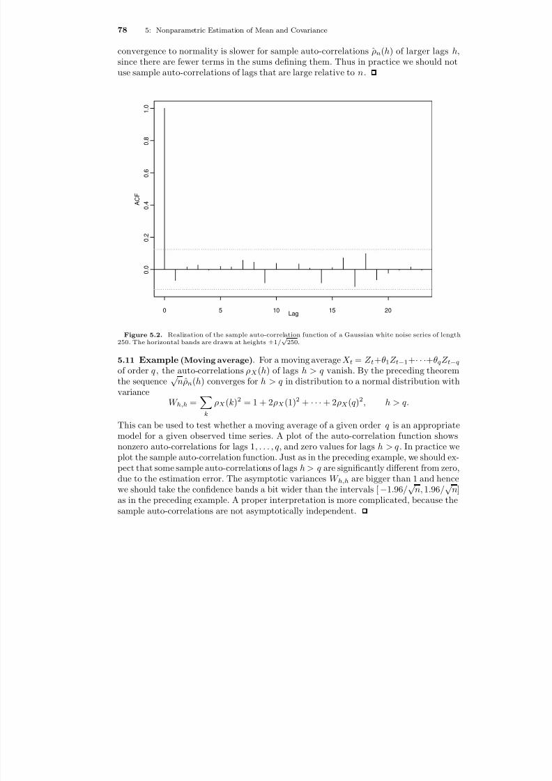
8/13/2019 van der Vaart: Time Series
http://slidepdf.com/reader/full/van-der-vaart-time-series 84/235
78 5: Nonparametric Estimation of Mean and Covariance
convergence to normality is slower for sample auto-correlations ˆ ρn (h) of larger lags h,since there are fewer terms in the sums dening them. Thus in practice we should notuse sample auto-correlations of lags that are large relative to n .
0 5 10 15 20
0
. 0
0 . 2
0 . 4
0 . 6
0 . 8
1 . 0
Lag
A C F
Figure 5.2. Realization of the sample auto-correlation function of a Gaussian white noise series of length250. The horizontal bands are drawn at heights ±1/ √ 250.
5.11 Example (Moving average) . For a moving average X t = Z t + θ1Z t−1 + · · ·+ θqZ t−qof order q , the auto-correlations ρX (h) of lags h > q vanish. By the preceding theoremthe sequence √ nρn (h) converges for h > q in distribution to a normal distribution withvariance
W h,h =k
ρX (k)2 = 1 + 2 ρX (1)2 +
· · ·+ 2 ρX (q )2 , h > q.
This can be used to test whether a moving average of a given order q is an appropriatemodel for a given observed time series. A plot of the auto-correlation function showsnonzero auto-correlations for lags 1 , . . . , q , and zero values for lags h > q . In practice weplot the sample auto-correlation function. Just as in the preceding example, we should ex-pect that some sample auto-correlations of lags h > q are signicantly different from zero,due to the estimation error. The asymptotic variances W h,h are bigger than 1 and hencewe should take the condence bands a bit wider than the intervals [ −1.96/ √ n, 1.96/ √ n]as in the preceding example. A proper interpretation is more complicated, because thesample auto-correlations are not asymptotically independent.

8/13/2019 van der Vaart: Time Series
http://slidepdf.com/reader/full/van-der-vaart-time-series 85/235
8/13/2019 van der Vaart: Time Series
http://slidepdf.com/reader/full/van-der-vaart-time-series 86/235
80 5: Nonparametric Estimation of Mean and Covariance
A nonparametric estimator ˆ α n (h) of αX (h) is obtained by replacing the auto-covariancefunction in this linear system by the sample auto-covariance function ˆ γ n . This yieldsestimators φ1 , . . . , φh of the prediction coefficients satisfying
γ n (0) γ n (1) · · · γ n (h −1)...
......
γ n (h −1) γ n (h −2) · · · γ n (0)
φ1...
φh
=γ n (1)
...γ n (h)
.
We dene a nonparametric estimator for αX (h) by α n (h) = φh . The function h → α n (h)is called the sample partial auto-covariance function .
If we write these two systems of equations as Γ φ = γ and Γφ = γ , respectively, thenwe obtain that
φ −φ = Γ−1 γ −Γ−1γ = Γ−1(γ −γ ) − Γ−1(Γ −Γ)Γ −1γ.
The sequences √ n(γ −γ ) and √ n(Γ −Γ) are jointly asymptotically normal by Theo-rem 5.8. With the help of Slutsky’s lemma we readily obtain the asymptotic normality of the sequence √ n(φ −φ) and hence of the sequence √ n α n (h) −α X (h) . The asymptoticcovariance matrix appears to be complicated, in general; we shall not derive it.
5.15 Example (Autoregression) . For the stationary solution to X t = φX t−1 + Z t
and |φ| < 1, the partial auto-correlations of lags h ≥ 2 vanish, by Example 2.34. InSection 11.1.2 it is shown that the sequence √ nα n (h) is asymptotically standard normallydistributed, for every h ≥2.
This result extends to the “causal” solution of the pth order auto-regressive schemeX t = φ1X t−1 + · · ·+ φ pX t− p + Z t and the auto-correlations of lags h > p . (The meaningof “causal” is explained in Chapter 8.) This property can be used to nd an appropriateorder p when tting an auto-regressive model to a given time series. The order is chosensuch that “most” of the sample auto-correlations of lags bigger than p are within the band[−1.96/ √ n, 1.96/ √ n]. A proper interpretation of “most” requires that the dependenceof the α n (h) is taken into consideration.

8/13/2019 van der Vaart: Time Series
http://slidepdf.com/reader/full/van-der-vaart-time-series 87/235
5.4: Partial Auto Correlations 81
0 5 10 15 20
0 . 0
0 . 2
0 . 4
Lag
P a r t i a
l A C F
Figure 5.4. Realization ( n = 250) of the partial auto-correlation function of the stationary solution toX t = 0 .5X t − 1 + 0 .2X t − 1 + Z t for a Gaussian white noise series.

8/13/2019 van der Vaart: Time Series
http://slidepdf.com/reader/full/van-der-vaart-time-series 88/235
6Spectral Theory
Let X t be a stationary, possibly complex, time series with auto-covariance function γ X .If the series h |γ X (h)| is convergent, then the series
(6.1) f X (λ) = 12π
h Z
γ X (h)e−ihλ ,
is absolutely convergent, uniformly in λ R . This function is called the spectral density of the time series X t . Because it is periodic with period 2 π it suffices to consider it onan interval of length 2 π, which we shall take to be ( −π, π ]. In the present context thevalues λ in this interval are often referred to as frequencies , for reasons that will becomeclear. By the uniform convergence, we can exchange the order of integral and sum whencomputing
π
−π eihλ f X (λ) dλ and we nd that, for every h Z ,
(6.2) γ X (h) = π
−πeihλ f X (λ) dλ.
Thus the spectral density f X determines the auto-covariance function, just as the auto-covariance function determines the spectral density.
6.1 EXERCISE. Verify the orthonormality of the trigonometric basis : π−π eihλ dλ = 0
for integers h = 0 and π
−π eihλ dλ = 2π for h = 0. Use this to prove the inversion formula (6.2), under the condition that h |γ X (h)| < ∞.
In mathematical analysis the series f X is called a Fourier series and the numbersγ X (h) are called the Fourier coefficients of f X . (The factor 1 / (2π) is sometimes omittedor replaced by another number, and the Fourier series is often dened as f X (−λ) ratherthan f X (λ), but this is inessential.) A central result in Fourier analysis is that the seriesin (6.1) converges in L2 (−π, π ], B , λ , and (6.2) is true, if and only if h |γ X (h)|2 < ∞.(See Lemma 6.3 below.) The latter condition is weaker than the absolute summability of the autocovariances. Furthermore, the converse of this statement is also true: if complex
8/13/2019 van der Vaart: Time Series
http://slidepdf.com/reader/full/van-der-vaart-time-series 89/235
6.1: Spectral Measures 83
numbers γ X (h) are dened by (6.2) from a given function f X L2 (−π, π ], B , λ , thenthis function can be recovered from (6.1), where the convergence is in L2 (−π, π ], B , λ .This involves the completeness of the trigonometric basis, consisting of the functionsλ → (2π)−1/ 2 e−ihλ , for h Z .
6.1 Spectral MeasuresThe requirement that the series h γ X (h) 2 is convergent means roughly that γ X (h) → 0as h → ±∞ at a “sufficiently fast” rate. In statistical terms it means that variables X tthat are widely separated in time must be approximately uncorrelated. This is not truefor every time series, and consequently not every time series possesses a spectral density.However, every stationary time series does have a “spectral measure”, by the followingtheorem.
6.2 Theorem (Herglotz) . For every stationary time series X t there exists a unique nite measure F X on (−π, π ] such that
γ X (h) = (−π,π ] eihλ
dF X (λ), h Z
.
Proof. Dene F n as the measure on [ −π, π ] with Lebesgue density equal to
f n (λ) = 12π
n
h = −n
γ X (h) 1 − |h|n
e−ihλ .
It is not immediately clear that this is a real-valued, nonnegative function, but thisfollows from the fact that
0 ≤ 12πn
varn
t =1
X t e−itλ = 12πn
n
s =1
n
t =1
cov(X s , X t )ei ( t−s )λ = f n (λ).
It is clear from the denition of f n that the numbers γ X (h) 1 − |h|/n are the Fouriercoefficients of f n for |h| ≤ n (and the remaining Fourier coefficients of f n are zero). Thus,by the inversion formula,
γ X (h) 1 − |h|n
= π
−πeihλ f n (λ) dλ =
π
−πeihλ dF n (λ), |h| ≤ n.
Setting h = 0 in this equation, we see that F n [−π, π ] = γ X (0) for every n . Thus, apartfrom multiplication by the constant γ X (0), the F n are probability distributions. Becausethe interval [ −π, π ] is compact, the sequence F n is uniformly tight. By Prohorov’s theorem

8/13/2019 van der Vaart: Time Series
http://slidepdf.com/reader/full/van-der-vaart-time-series 90/235
84 6: Spectral Theory
there exists a subsequence F n that converges weakly to a distribution F on [−π, π ].Because λ → eihλ is a continuous function, it follows by the portmanteau lemma that
[−π,π ]eihλ dF (λ) = lim
n →∞ [−π,π ]eihλ dF n (λ) = γ X (h),
by the preceding display. If F puts a positive mass at −π, we can move this to the pointπ without affecting this identity, since e−ihπ = eihπ for every h Z . The resulting F satises the requirements for F X .
That this F is unique can be proved using the fact that the linear span of the func-tions λ → eihλ is uniformly dense in the set of continuous, periodic functions (see Rudin,Theorem 4.25; in fact, by Fejer’s theorem, the Cesaro sums of the Fourier series of acontinuous, periodic function converge uniformly). Using this fact, we see that equality
h dF = h dG, for two measures F and G and every function h of the form λ → eiλh ,implies equality for any continuous, periodic function h. Using the monotone and/or dom-inated convergence theorems, this can be extended to any bounded measurable function.This implies that F = G.
The measure F X is called the spectral measure of the time series X t . If the spectralmeasure F X admits a density f X relative to the Lebesgue measure, then the latter iscalled the spectral density . A sufficient condition for this is that the square summabilityof the square autocovariances. Then the spectral density is the Fourier series (6.1), withFourier coefficients γ X (h).
6.3 Lemma. If γ X (h) 2 < ∞, then the series (6.1) converges in L2 (−π, π ], B , λ ,and denes a density of F X relative to Lebesgue measure.
Proof. The orthonormality of the trigonometric basis shows that, for any m ≤ n,
π
−π m ≤|h |≤n
γ X (h)e−ihλ2
dλ =m ≤|g|≤n m ≤|h |≤n
γ X (h)γ X (g) π
−πei (h −g)λ dλ
= 2 πm ≤|h |≤n
γ X (h) 2 .
Thus the convergence of the series
γ
X(h) 2 is equivalent to the convergence of the
series (6.1) in L2 (−π, π ], B , λ .Next the continuity of the inner product in L2 (−π, π ], B , λ allows exchanging the
order of integration and summation in π
−π eigλh γ X (h)e−ihλ dλ. Then (6.2) follows
from the orthonormality of the trigonometric basis.
6.4 EXERCISE. Show that the spectral density of a real-valued time series withh γ X (h) < ∞ is symmetric about zero.
* 6.5 EXERCISE. Show that the spectral measure of a real-valued time series is symmetricabout zero, apart from a possible point mass at π. [Hint: Use the uniqueness of a spectralmeasure.]
8/13/2019 van der Vaart: Time Series
http://slidepdf.com/reader/full/van-der-vaart-time-series 91/235
6.1: Spectral Measures 85
6.6 Example (White noise) . The covariance function of a white noise sequence X t is0 for h = 0. Thus the Fourier series dening the spectral density has only one term andreduces to
f X (λ) = 12π
γ X (0) .
The spectral measure is the uniform measure with total mass γ X (0). Hence “a whitenoise series contains all possible frequencies in an equal amount”.
6.7 Example (Deterministic trigonometric series) . Let X t = A cos(λt )+ B sin(λt ) formean-zero, uncorrelated variables A and B of variance σ2 , and λ (0, π ). By Example 1.5the covariance function is given by
γ X (h) = σ2 cos(hλ ) = σ2 12 (eiλh + e−iλh ).
It follows that the spectral measure F X is the discrete 2-point measure with F X λ =F X −λ= σ2/ 2.
Because the time series is real, the point mass at −λ does not really count: becausethe spectral measure of a real time series is symmetric, the point −λ must be therebecause λ is there. The form of the spectral measure and the fact that the time series inthis example is a trigonometric series of frequency λ, are good motivation for referringto the values λ as “frequencies”.
6.8 EXERCISE.(i) Show that the spectral measure of the sum X t + Y t of two uncorrelated time series
is the sum of the spectral measures of X t and Y t .(ii) Construct a time series with spectral measure equal to a symmetric discrete measure
on the points ±λ1 , ±λ2 , . . . , ±λk with 0 < λ 1 < · · · < λ k < π .(iii) Construct a time series with spectral measure the 1-point measure with F X 0= σ2 .(iv) Same question, but now with F X π= σ2 .
* 6.9 EXERCISE. Show that every nite measure on ( −π, π ] is the spectral measure of some stationary time series.
The spectrum of a time series is an important theoretical concept, but it is alsoan important practical tool to gain insight in periodicities in the data. Inference usingthe spectrum is called spectral analysis or analysis in the frequency domain as opposedto “ordinary” analysis, which is in the time domain . It depends on the subject eldwhether a spectral analysis is useful. If there are periodicities present in a time series,then a spectral analysis will reveal these. However, in general we should not have toogreat expectations of the insight offered by the spectrum. For instance, the interpretationof the spectrum of economic time series may be complicated, or even unclear, due to thefact that all possible frequencies are present to some nontrivial extent.
The idea of a spectral analysis is to view the consecutive values
. . . , X −1 , X 0 , X 1 , X 2 , . . .

8/13/2019 van der Vaart: Time Series
http://slidepdf.com/reader/full/van-der-vaart-time-series 92/235
86 6: Spectral Theory
of a time series as a random function X : Z R → R , and to write this as a weightedsum (or integral) of trigonometric functions t → cos λt or t → sin λt of different frequen-cies λ. In simple cases nitely many frequencies suffice, whereas in other situations allfrequencies λ (−π, π ] are needed to give a full description, and the “weighted sum”becomes an integral. Two extreme examples are provided by a deterministic trigonomet-ric series (which incorporates a single frequency) and a white noise series (which has allfrequencies in equal amounts). The spectral measure gives the weights of the differentfrequencies in the sum.
We shall derive the spectral decomposition , the theoretical basis for this interpreta-tion, in Section 6.4. Another method to gain insight in the interpretation of a spectrumis to consider its transformation under ltering. The term “ltering” stems from the eldof signal processing, where a lter takes the form of an physical device that lters outcertain frequencies from a given electric current. For us, a (linear) lter will remain aninnite moving average as dened in Chapter 1. For a given lter with lter coefficientsψj the function ψ(λ) = j ψj e−ijλ is called the transfer function of the lter.
6.10 Theorem. Let X t be a stationary time series with spectral measure F X and letj |ψj | < ∞. Then Y t = j ψj X t−j has spectral measure F Y given by, with ψ the
transfer function,
dF Y (λ) = ψ(λ) 2 dF X (λ).
Proof. According to Lemma 1.28(iii) (if necessary extended to complex-valued lters),the series Y t is stationary with auto-covariance function
γ Y (h) =k l
ψk ψ lγ X (h −k + l) =k l
ψk ψl ei (h −k+ l)λ dF X (λ).
By the dominated convergence theorem we are allowed to change the order of (double)summation and integration. Next we can rewrite the right side as ψ(λ) 2 eihλ dF X (λ).This proves the theorem, in view of Theorem 6.2 and the uniqueness of the spectralmeasure.
6.11 Example (Moving average) . A white noise process Z t has a constant spectraldensity σ2/ (2π). By the preceding theorem the moving average X t = Z t + θZ t−1 hasspectral density
f X (λ) = |1 + θe−iλ |2 σ2
2π = (1 + 2 θ cos λ + θ2)
σ2
2π.
If θ > 0, then the small frequencies dominate, whereas the bigger frequencies are moreimportant if θ < 0. This suggests that the sample paths of this time series will be morewiggly if θ < 0. However, in both cases all frequencies are present in the signal.

8/13/2019 van der Vaart: Time Series
http://slidepdf.com/reader/full/van-der-vaart-time-series 93/235
6.1: Spectral Measures 87
0.0 0.5 1.0 1.5 2.0 2.5 3.0
- 6
- 4
- 2
0
2
s p e c t r u m
Figure 6.1. Spectral density of the moving average X t = Z t + .5Z t − 1 . (Vertical scale in decibels.)
6.12 Example. The complex-valued process X t = Ae iλt for a mean zero variable A andλ (−π, π ] has covariance function
γ X (h) = cov( Aeiλ ( t + h ) , Aeiλt ) = eihλ E|A|2 .
The corresponding spectral measure is the 1-point measure F X with F X λ = E |A|2 .Therefore, the ltered series Y t = j ψj X t−j has spectral measure the 1-point measurewith F Y λ = ψ(λ) 2E|A|2 . By direct calculation we nd that
Y t =j
ψj Aeiλ ( t−j ) = Ae iλt ψ(λ) = ψ(λ)X t .
This suggests an interpretation for the term “transfer function”. Filtering a “pure signal”Aeitλ of a single frequency apparently yields another signal of the same single frequency,but the amplitude of the signal changes by multiplication with the factor ψ(λ). If ψ(λ) =0, then the frequency is “not transmitted”, whereas values of ψ(λ) bigger or smallerthan 1 mean that the frequency λ is amplied or weakened.
6.13 EXERCISE. Find the spectral measure of X t = Ae iλt for λ not necessarily belong-ing to (−π, π ].

8/13/2019 van der Vaart: Time Series
http://slidepdf.com/reader/full/van-der-vaart-time-series 94/235
88 6: Spectral Theory
To give a further interpretation to the spectral measure consider a band pass lter .This is a lter with transfer function of the form
ψ(λ) = 0, if |λ −λ0 | > δ ,1, if |λ −λ0 | ≤δ ,
for a xed frequency λ0 and xed band width 2δ . According to Example 6.12 this lter“kills” all the signals Aeiλt of frequencies λ outside the interval [ λ0 − δ, λ0 + δ ] andtransmits all signals Ae itλ for λ inside this range unchanged. The spectral density of theltered signal Y t = j ψj X t−j relates to the spectral density of the original signal X t(if there exists one) as
f Y (λ) = ψ(λ) 2 f X (λ) = 0, if |λ −λ0| > δ ,f X (λ), if |λ −λ0| ≤ δ .
Now think of X t as a signal composed of many frequencies. The band pass lter transmitsonly the subsignals of frequencies in the interval [ λ0 −δ, λ0 + δ ]. This explains that thespectral density of the ltered sequence Y t vanishes outside this interval. For small δ > 0,
var Y t = γ Y (0) = π
−πf Y (λ) dλ =
λ 0 + δ
λ 0 −δf X (λ) dλ ≈ 2δf X (λ0 ).
We interprete this as saying that f X (λ0) is proportional to the variance of the subsignalsin X t of frequency λ0 . The total variance var X t = γ X (0) =
π−π f X (λ) dλ in the signal
X t is the total area under the spectral density. This can be viewed as the sum of thevariances of the subsignals of frequencies λ, the area under f X between λ0 −δ and λ0 + δ being the variance of the subsignals of frequencies in this interval.
A band pass lter is a theoretical lter: in practice it is not possible to lter outan exact range of frequencies. Electronic devices will not lter frequencies close to theborders of the band correctly. On a computer only nite lters can be implemented (theones with only nitely many nonzero lter coefficients ψj ). These have transfer functionsthat are a nite linear combination of sines and cosines, and hence are smooth and cannot jump, in contrast to the indicator function corresponding to a band pass lter.
The lter coefficients ψj relate to the transfer function ψ(λ) in the same way asthe auto-covariances γ X (h) relate to the spectral density f X (h), apart from a factor 2 π.
Thus, to nd the lter coefficients of a given transfer function ψ, it suffices to apply theFourier inversion formulaψj =
12π
π
−πeijλ ψ(λ) dλ.
6.14 EXERCISE. Show that the lter coefficients of a band pass lter with ( l0 −δ, λ0 +δ ) (0, π ) are given by ψj = eiλ 0 j sin(δj )/ (πj ).
6.15 Example (Low frequency and trend) . An apparent trend in observed dataX 1 , . . . , X n could be modelled as a real trend in a nonstationary time series, but couldalternatively be viewed as the beginning of a long cycle. In practice, where we get tosee only a nite stretch of a time series, low frequency cycles and slowly moving trends

8/13/2019 van der Vaart: Time Series
http://slidepdf.com/reader/full/van-der-vaart-time-series 95/235
6.1: Spectral Measures 89
cannot be discriminated. It was seen in Chapter 1 that differencing Y t = X t −X t−1 of a time series X t removes a linear trend, and repeated differencing removes higher orderpolynomial trends. In view of the preceding observation the differencing lter shouldremove, to a certain extent, low frequencies.
The differencing lter has transfer function
ψ(λ) = 1 −e−iλ = 2 ie−iλ/ 2 sin λ2
.
The absolute value ψ(λ) of this transfer function increases from 0 at 0 to its maximumvalue at π. Thus, indeed, it lters away low frequencies, albeit only with partial success.
0.0 0.5 1.0 1.5 2.0 2.5 3.0
0 . 0
0 . 5
1 . 0
1 . 5
2 . 0
Figure 6.2. Absolute value of the transfer function of the difference lter.
6.16 Example (Averaging) . The averaging lter Y t = (2 M + 1) −1 M
j = −M X t−j hastransfer function
ψ(λ) = 1
2M + 1
M
j = −M
e−ijλ = sin (M + 1
2 )λ(2M + 1) sin( 1
2 λ).
(The expression on the right is dened by continuity, as 1, at λ = 0.) This functionis proportional to the Dirichlet kernel , which is the function obtained by replacing thefactor 2 M + 1 by 2π. From a picture of this kernel we conclude that averaging removeshigh frequencies to a certain extent (and in an uneven manner depending on M ), butretains low frequencies.

8/13/2019 van der Vaart: Time Series
http://slidepdf.com/reader/full/van-der-vaart-time-series 96/235
90 6: Spectral Theory
0.0 0.5 1.0 1.5 2.0 2.5 3.0
0
1
2
3
s i n ( u * 1 0
. 5 ) / s i n ( u / 2 ) / ( 2 * p
i )
Figure 6.3. Dirichlet kernel of order M = 10.
6.17 EXERCISE. Express the variance of Y t in the preceding example in ψ and thespectral density of the time series X t (assuming that there is one). What happens if M → ∞? Which conclusion can you draw? Does this remain true if the series X t doesnot have a spectral density? [Verify that |ψ(λ)| ≤ 1 for every λ and M , and that ψ(λ) → 0as M → ∞ for every 0.]
6.18 EXERCISE. Find the transfer function of the lter Y t = X t −X t−12 . Interpretethe result.
Instead of in terms of frequencies we can also think in periods . A series of the formt → eiλt repeats itself after 2 π/λ instants of time. Therefore, the period is dened as
period = 2π
frequency.
Most monthly time series (one observation per month) have a period effect of 12 months.If so, this will be visible as a peak in the spectrum at the frequency 2 π/ 12 = π/ 6.† Often
† That this is a complicatednumber is an inconvenient consequence of our convention to dene the spectrumon the interval ( −π, π ]. This can be repaired. For instance, the Splus package produces spectral plots with thefrequencies rescaled to the interval ( −1
2 , 12 ]. Then a 12-month period gives a peak at 1 / 12.

8/13/2019 van der Vaart: Time Series
http://slidepdf.com/reader/full/van-der-vaart-time-series 97/235
6.2: Aliasing 91
the 12-month cycle is not completely regular. This may produce additional (but smaller)peaks at the harmonic frequencies 2π/ 6, 3π/ 6, . . ., or π/ 12, π/ 18, . . ..
It is surprising at rst that the highest possible frequency is π, the so-called Nyquist frequency . This is caused by the fact that the series is measured only at discrete timepoints. Very rapid uctuations fall completely between the measurement times and hencecannot be observed. The Nyquist frequency π corresponds to a period of 2 π/π = 2 timeinstants and this is clearly the smallest period that is observable. The next section shedsmore light on this.
* 6.2 Aliasing
In many situations in practice a time series arises by measuring an underlying continuoustime process, an operation called sampling . The choice of the time instants at whichmeasurements are taken is up to us, and we have to choose a sampling frequency . Themore we sample the better, of course, but practical considerations, such as computerstorage of the data, will impose restrictions. In this section we study the effect of samplingon the spectrum of a time series.
Consider a time series ( X t : t Z ) obtained by sampling a continuous time stochastic
process (Y t : t R ) at times −δ, 0, δ, 2δ , . . . for a sampling interval δ > 0: X t = Y tδ . Thecontinuous time process Y t is said to be second order stationary if its expectation isconstant and the autovariances cov( Y t + h , Y t ) do not depend on t, so that its (continuoustime) autocovariance function can be dened by, for h R ,
γ Y (h) = cov( Y t + h , Y t ).
By Bochner’s theorem , provided that it is continuous, such a covariance function canalways be represented by a nite Borel measure F Y on R in the form
γ Y (h) = ∞−∞eihλ dF Y (λ), h R .
This is similar to Herglotz’ theorem, the important difference being that the represen-tation uses all frequencies in R , not just an interval of length 2 π, and is valid for thecontinuum of lags h R .‡
6.19 Lemma. The skeleton (X t : t Z ) = ( Y tδ : t Z ) of a continuous time stationary process (Y t : t Z ) with spectral measure F Y possesses spectral measure F X given by
F X (B ) =k Z
F Y B + k 2π
δ .
‡ For a proof of Bochner’s theorem, along the lines of the proof of Herglotz theorem, see pages 275–277 of Gnedenko (1962).

8/13/2019 van der Vaart: Time Series
http://slidepdf.com/reader/full/van-der-vaart-time-series 98/235

8/13/2019 van der Vaart: Time Series
http://slidepdf.com/reader/full/van-der-vaart-time-series 99/235
6.4: Spectral Decomposition 93
Proof. For 0 ≤ m ≤ n let ψm,nj be equal to ψj for m ≤ | j | ≤ n and be 0 otherwise, and
dene Y m,nt as the series X t ltered by the coefficients ψm,n
j . Then certainly j |ψm,nj | <
∞ for every xed pair ( m, n ) and hence we can apply Lemma 1.28 and Theorem 6.10 tothe series Y m,n
t . This yields
Em ≤|j |≤n
ψj X t−j2
= E |Y m,nt |2 = γ Y m,n (0)
= (−π,π ] dF Y m,n = (−π,π ] m ≤|j |≤n ψj e−iλj
2
dF X (λ).
The left side converges to zero for m, n → ∞ if and only if the partial sums of the seriesY t = j ψj X t−j form a Cauchy sequence in L2(Ω, U , P). The right side converges to zeroif and only if the partial sums of the sequence j ψj e−iλj form a Cauchy sequence inL2(F X ). The rst assertion of the theorem now follows, because both spaces are complete.
To prove the second assertion, we rst note that, by Theorem 6.10,
cov
|j |≤n
ψj X t + h −j ,
|j |≤n
ψj X t−j = γ Y 0 ,n (h) = (−π,π ] |j |≤n
ψj e−iλj2eihλ dF X (λ).
We now take limits of the left and right sides as n → ∞ to nd that γ Y (h) =
(
−π,π ] ψ(λ) 2 eihλ dF X (λ), for every h.
6.21 Example. If the lter coefficients satisfy j |ψj |2 < ∞ (which is weaker thanabsolute convergence), then the series j ψj e−ijλ converges in L2 (−π, π ], B , λ . Conse-quently, the series also converges in L2(F X ) for every spectral measure F X that possessesa bounded density.
Thus, in many cases a sequence of square-summable coefficients denes a valid lter.A particular example is a band pass lter, for which |ψj | = O(1/ | j |) as j → ±∞.
* 6.4 Spectral Decomposition
In the preceding section we interpreted the mass F X (I ) that the spectral distributiongives to an interval I as the size of the contribution of the components of frequenciesλ I to the signal t → X t . In this section we give a precise mathematical meaning tothis idea. We show that a given stationary time series X t can be written as a randomlyweighted sum of single frequency signals eiλt .
This decomposition is simple in the case of a discrete spectral measure. For givenuncorrelated, zero-mean random variables Z 1 , . . . , Z k and numbers λ 1 , . . . , λ k (−π, π ]the process
X t =k
j =1
Z j eiλ j t

8/13/2019 van der Vaart: Time Series
http://slidepdf.com/reader/full/van-der-vaart-time-series 100/235
94 6: Spectral Theory
possesses as spectral measure F X the discrete measure with point masses of sizesF X λ j = E |Z j |2 at the frequencies λ1 , . . . , λ k (and no other mass). The series X t isthe sum of uncorrelated, single-frequency signals of stochastic amplitudes |Z j |. This iscalled the spectral decomposition of the series X t . We prove below that this construc-tion can be reversed: given a mean zero, stationary time series X t with discrete spectralmeasure as given, there exist mean zero uncorrelated (complex-valued) random variablesZ 1 , . . . , Z k with variances F X λ j such that the decomposition is valid.
This justies the interpretation of the spectrum given in the preceding section. The
possibility of the decomposition is surprising in that the spectral measure only involvesthe auto-covariance function of a time series, whereas the spectral decomposition is adecomposition of the sample paths of the time series: if the series X t is dened on agiven probability space (Ω , U , P), then so are the random variables Z j and the precedingspectral decomposition may be understood as being valid for (almost) every ω Ω. Thiscan be true, of course, only if the variables Z 1 , . . . , Z k also have other properties besidesthe ones described. The spectral theorem below does not give any information aboutthese further properties. For instance, even though uncorrelated, the Z j need not beindependent. This restricts the usefulness of the spectral decomposition, but we couldnot expect more. The spectrum only involves the second moment properties of the timeseries, and thus leaves most of the distribution of the series undescribed. An importantexception to this rule is if the series X t is Gaussian. Then the rst and second moments,and hence the mean and the spectral distribution, completely describe the distributionof the series X t .
The spectral decomposition is not restricted to time series’ with discrete spectralmeasures. However, in general, the spectral decomposition involves a continuum of fre-quencies and the sum becomes an integral
X t = (−π,π ]eiλt dZ (λ).
A technical complication is that such an integral, relative to a “random measure” Z , isnot dened in ordinary measure theory. We must rst give it a meaning.
6.22 Denition. A random measure with orthogonal increments Z is a collectionZ (B ): B B of mean zero, complex random variables Z (B ) indexed by the Borel sets B in (−π, π ] dened on some probability space (Ω, U , P) such that, for some nite Borel measure µ on (−π, π ],
cov Z (B1), Z (B2) = µ(B1 ∩B2), every B1 , B2 B .
This denition does not appear to include a basic requirement of a measure: thatthe measure of a countable union of disjoint sets is the sum of the measures of theindividual sets. However, this is implied by the covariance property, which says that thelinear extension of the map 1 B → Z (B ) is an isometry from L2(µ) into L2(Ω, U , P).

8/13/2019 van der Vaart: Time Series
http://slidepdf.com/reader/full/van-der-vaart-time-series 101/235
6.4: Spectral Decomposition 95
6.23 EXERCISE. Let Z be a random measure with orthogonal increments. Show thatZ ( j B j ) = j Z (B j ) in mean square, whenever B1 , B2 , . . . is a sequence of pairwisedisjoint Borel sets.
6.24 EXERCISE. Let Z be a random measure with orthogonal increments and deneZ λ = Z (−π, λ ]. Show that ( Z λ : λ (−π, π ]) is a stochastic process with uncorrelatedincrements: for λ1 < λ 2 ≤ λ3 < λ 4 the variables Z λ 4 −Z λ 3 and Z λ 2 −Z λ 1 are uncorrelated.This explains the phrase “with orthogonal increments”.
* 6.25 EXERCISE. Suppose that Z λ is a mean zero stochastic process with nite secondmoments and uncorrelated increments. Show that this process corresponds to a randommeasure with orthogonal increments as in the preceding exercise. [This asks you toreconstruct the random measure Z from the weights Z λ = Z (−π, λ ] it gives to cells,similarly as an ordinary measure can be reconstructed from its distribution function.The construction below will immediately give us the complete random measure as inDenition 6.22. So it is not really helpful to go through the somewhat tedious details of this construction, although many authors start from distribution functions rather thanmeasures.]
Next we dene an “integral” f dZ for given functions f : (−π, π ] → C . For anindicator function f = 1B of a Borel set B, we dene, in analogy with an ordinary
integral, 1B dZ = Z (B ). Because we wish the integral to be linear, we are lead to thedenition
j
α j 1B j dZ =j
α j Z (B j ),
for every nite collections of complex numbers αj and Borel sets Bj . This determinesthe integral for many, but not all functions f . We extend its domain by continuity:we require that f n dZ → f dZ whenever f n → f in L2(µ). The following lemmashows that these denitions and requirements can be consistently made, and serves as adenition of f dZ .
6.26 Lemma. For every random measure with orthogonal increments Z there exists a unique map, denoted f →
f dZ , from L2(µ) into L2(Ω, U , P) with the properties
(i)
1B dZ = Z (B );
(ii) (αf + βg) dZ = α f dZ + β g dZ ;(iii) E f dZ 2 = |f |
2 dµ.In other words, the map f → f dZ is a linear isometry such that 1B → Z (B ).
Proof. By the dening property of Z , for any complex numbers α i and Borel sets B i ,
Ek
i =1
α i Z (B i )2
=i j
α i α j cov Z (B i ), Z (B j ) = k
j =1
α i 1B i
2dµ.
For f a simple function of the form f = i α i 1B i , we dene f dZ as i α i Z (B i ).This is well dened, for, if f also has the representation f = j β j 1D j , then

8/13/2019 van der Vaart: Time Series
http://slidepdf.com/reader/full/van-der-vaart-time-series 102/235
96 6: Spectral Theory
i α i Z (B i ) = j β j Z (D j ) almost surely. This follows by applying the preceding identityto i α i Z (B i ) − j β j Z (D j ).
The “integral” f dZ that is now dened on the domain of all simple functions f trivially satises (i) and (ii), while (iii) is exactly the identity in the preceding display.The proof is complete upon showing that the map f → f dZ can be extended fromthe domain of simple functions to the domain L2(µ), meanwhile retaining the properties(i)–(iii).
We extend the map by continuity. For every f
L2(µ) there exists a sequence of
simple functions f n such that |f n −f |2 dµ → 0. We dene f dµ as the limit of thesequence f n dZ . This is well dened. First, the limit exists, because, by the linearity of the integral and the identity,
E f n dµ − f m dµ|2 = |f n −f m |2 dµ,
since f n −f m is a simple function. Because f n is a Cauchy sequence in L2(µ), the rightside converges to zero as m, n → ∞. We conclude that f n dZ is a Cauchy sequencein L2(Ω, U , P) and hence it has a limit by the completeness of this space. Second, thedenition of f dZ does not depend on the particular sequence f n → f we use. Thisfollows, because given another sequence of simple functions gn → f , we have |f n −gn
|2 dµ
→ 0 and hence E
f n dZ
− gn dZ
2
→ 0.
We conclude the proof by noting that the properties (i)–(iii) are retained undertaking limits.
6.27 Denition (Stochastic integral) . The stochastic integral f dZ of a function f L2(µ) relative to a random measure with orthogonal increments Z as in Denition 6.22 is given by the map dened in Lemma 6.26.
Warning. This integral is constructed in a similar way as the It o integral in stochas-tic analysis, but it is not the same. The process Z in the decomposition Z (0, λ] = Z λ −Z 0of a random measure with orthogonal increments is not necessarily a semimartingale. Onthe other hand, the integral f dZ is dened here only for deterministic integrands.
6.28 EXERCISE. Show that a linear isometry Φ: H 1
→ H 2 between two Hilbert spaces
H 1 and H 2 retains inner products, i.e. Φ(f 1), Φ(f 2) 2 = f 1 , f 2 1 . Conclude thatcov f dZ, g dZ = fg dµ.
We are now ready to derive the spectral decomposition for a general stationary timeseries X t . Let L2(X t : t Z ) be the closed, linear span of the elements of the time seriesin L2(Ω, U , P) (i.e. the closure of the linear span of the set X t : t Z ).
6.29 Theorem. For any mean zero stationary time series X t with spectral distributionF X there exists a random measure Z with orthogonal increments relative to the measure F X such that Z (B ): B B L2(X t : t Z ) and such that X t = e
iλt dZ (λ) almostsurely for every t Z .
8/13/2019 van der Vaart: Time Series
http://slidepdf.com/reader/full/van-der-vaart-time-series 103/235
6.4: Spectral Decomposition 97
Proof. By the denition of the spectral measure F X we have, for every nite collectionsof complex numbers α j and integers t j ,
E α j X t j
2=
i j
α i α j γ X (t i −t j ) = α j eit j λ2
dF X (λ).
Now dene a map Φ: L2(F X ) → L2(X t : t Z ) as follows. For f of the form f =j α j eit j λ dene Φ(f ) =
α j X t j . By the preceding identity this is well dened.
(Check!) Furthermore, Φ is a linear isometry. By the same arguments as in the pre-ceding lemma, it can be extended to a linear isometry on the closure of the space of all functions j α j eit j λ . By Fejer’s theorem from Fourier theory, this closure containsat least all Lipschitz periodic functions. By measure theory this collection is dense inL2(F X ). Thus the closure is all of L2(F X ). In particular, it contains all indicator func-tions 1B of Borel sets B . Dene Z (B ) = Φ(1 B ). Because Φ is a linear isometry, it retainsinner products and hence
cov Z (B1), Z (B2) = Φ(1B 1 ), Φ(1B 2 ) = 1B 1 1B 2 dF X .
This shows that Z is a random measure with orthogonal increments. By denition
j
α j 1B j dZ =j
α j Z (B j ) = α j Φ(1B j ) = Φj
α j 1B j .
Thus f dZ = Φ( f ) for every simple function f . Both sides of this identity are linearisometries when seen as functions of f L2(F X ). Hence the identity extends to all f L2(F X ). In particular, we obtain e
itλ dZ (λ) = Φ( eitλ ) = X t on choosing f (λ) = eitλ .
Thus we have managed to give a precise mathematical formulation to the spectraldecomposition
X t = (−π,π ]eitλ dZ (λ)
of a mean zero stationary time series X t . The denition may seem a bit involved. (Itmay even seem that giving a meaning to the representation was harder than proving its
validity.) An insightful interpretation is obtained by approximation through Riemannsums. Given a partition −π = λ0,k < λ 1,k < · · · < λ k,k = π and a xed time t Z ,consider the function λ → f k (λ) that is piecewise constant, and takes the value eitλ j,k
on the interval ( λ j −1,k , λ j,k ]. If the partitions are chosen such that the mesh widthof the partitions converges to zero as k → ∞, then f k (λ) − eitλ converges to zero,uniformly in λ (−π, π ], by the uniform continuity of the function λ → eitλ , and hencef k (λ) → eitλ in L2(F X ). Because the stochastic integral f → f dZ is linear, we have
f k dZ = j eitλ j,k Z (λ j −1,k λ j,k ] and because it is an isometry, we nd
E X t −k
j =1
eitλ j,k Z (λ j −1,k , λ j,k ]2
= eitλ −f k (λ) 2 dF X (λ) → 0.
8/13/2019 van der Vaart: Time Series
http://slidepdf.com/reader/full/van-der-vaart-time-series 104/235
98 6: Spectral Theory
Because the intervals ( λ j −1,k , λ j,k ] are pairwise disjoint, the random variables Z j : =Z (λ j −1,k , λ j,k ] are uncorrelated, by the dening property of an orthogonal random mea-sure. Thus the time series X t can be approximated by a time series of the form j Z j eitλ j ,as in the introduction of this section. The spectral measure F X (λ j −1,k , λ j,k ] of the interval(λ j −1,k , λ j,k ] is the variance of the random weight Z j in this decomposition.
6.30 Example. If the spectral measure F X is discrete with support points λ1 , . . . , λ k ,then the integral on the right in the preceding display (with λj,k = λj ) is identically
zero. In that case X t = j Z j e
iλ j t
almost surely for every t , where Z j = Z λ j . (Notethat Z (λ j −1 , λ j ) = 0).
6.31 Example. If the time series X t is Gaussian, then all variables in the linear spanof the X t are normally distributed (possibly degenerate) and hence all variables inL2(X t : t Z ) are normally distributed. In that case the variables Z (B ) obtained from therandom measure Z of the spectral decomposition of X t are jointly normally distributed.The zero correlation of two variables Z (B1) and Z (B2) for disjoint sets B1 and B2 nowimplies independence of these variables.
Theorem 6.10 shows how a spectral measure changes under ltering. There is acorresponding result for the spectral decomposition.
6.32 Theorem. Let X t be a mean zero, stationary time series with spectral measure
F X and associated random measure Z X , dened on some probability space (Ω, U , P) . If ψ(λ) = j ψj e−iλj converges in L2(F X ), then Y t = j ψj X t−j converges in L2(Ω, U , P)and has spectral measure F Y and associated random measure Z Y such that, for every f L2(F Y ),
f dZ Y = fψdZ X .
Proof. The series Y t converges by Theorem 6.10, and the spectral measure F Y hasdensity ψ(λ) 2 relative to F X . By denition,
eitλ dZ Y (λ) = Y t =j
ψj ei ( t−j )λ dZ X (λ) = eitλ ψ(λ) dZ X (λ),
where in the last step changing the order of integration and summation is justied by the
convergence of the series j ψj e
i ( t
−j )λ
in L2(F X ) and the continuity of the stochasticintegral f → f dZ X . We conclude that the identity of the theorem is satised for everyf of the form f (λ) = eitλ . Both sides of the identity are linear in f and isometries onthe domain f L2(F Y ). Because the linear span of the functions λ → eitλ for t Z isdense in L2(F Y ), the identity extends to all of L2(F Y ).
The spectral decomposition X t = eiλt dZ (λ) is valid for both real and complex time
series. Because the representation is in terms of the complex functions eitλ , the spectralrandom measure Z of a real time series is typically complex valued. The following lemmashows that it is complex-conjugate. Abbreviate f dZ (λ) to Z (f ), and given a functionf : (−π, π ] → C let f − be the reection (of its periodic extension): f −(λ) = f (−λ) forλ (−π, π ) and f −(π) = f (π).
8/13/2019 van der Vaart: Time Series
http://slidepdf.com/reader/full/van-der-vaart-time-series 105/235
6.4: Spectral Decomposition 99
6.33 Lemma. The spectral random measure of a real time series X t satises Z (f ) =Z (f −) almost surely, for every f L(F X ). In particular Z (B ) = Z (−B ) almost surely,for every Borel set B (−π, π ). Furthermore, for any f , g L2(F X ),
E Re Z (f ) Re Z (g) = 14 (f + f −)(g + g−) dF X ,
E Re Z (f ) Im Z (g) = 14 (f + f −)(g −g−) dF X ,
E Im Z (f ) Im Z (g) = 14 (f −f −)(g −g−) dF X .
In particular, if f and g are real and vanish outside (0, π), then E Re Z (f ) Im Z (g) = 0and E Re Z (f ) Re Z (g) = EIm Z (f ) Im Z (g).
Proof. If the Fourier series j f j eitλ , where f j = (2 π)−1
e−ijλ f (λ) dλ , converges inL2(F X ) to the function f , then by the continuity of the random spectral measure
Z (f ) =j
f j Z (eijλ ) =j
f j X j ,
where the convergence of the innite series’ is in L2(X t : t Z ). Because the Fouriercoefficients of f − are equal to f j , it then follows that
Z (f ) = f j X j = Z (f −).
This proves the conjugate symmetry of Z for functions f of this type. The convergence(and hence the conjugate symmetry) is certainly true for every periodic, Lipschitz func-tion f , for which the convergence of the Fourier series is uniform. A general f can beapproximated in L2(F X ) by a sequence f n of Lipschitz, periodic functions, and then thesequence f n − tends in L2(F X ) to f −, in view of the symmetry of F X . Thus the conjugatesymmetry extends to any such function.
The expressions for the second moments of the real and imaginary parts followupon writing Re Z (f ) = 1
2 Z (f ) + Z (f ) = 12 Z (f + f −) and Im Z (f ) = 1
2 Z (f ) −Z (f ) = 1
2 Z (f −f −). In the particular case that f and g are real and vanish outside(0, π), the function f + f − is symmetric, the function g − g− is anti-symmetric, and(f + f
−)(g + g
− = ( f
−f −
)(g
−g−
). Together with the symmetry of F X
this yields thelast assertion.
The last assertion of the preceding lemma shows that the random vectorsRe Z (f 1), . . . , Re Z (f k ) and Im Z (f 1), . . . , Im Z (f k ) are uncorrelated and have equal
covariance matrix, for any real functions f 1 , . . . , f k in L2(F X ) that vanish outside (0 , π).This implies that the vector of combined real and imaginary parts of the complex randomvector Z (f 1), . . . , Z (f k ) possesses a covariance matrix of the form (1.2), for functionsf 1 , . . . , f k of the special type considered, and then also for general functions that vanishat 0 and π by the linearity of Z in f . In particular, if the time series X t is real and Gaus-sian, then the complex random vector Z (f 1), . . . , Z (f k ) possesses a complex normaldistribution N (0, Σ) for Σ the matrix with ( i, j )th element f i f j dF X .
8/13/2019 van der Vaart: Time Series
http://slidepdf.com/reader/full/van-der-vaart-time-series 106/235
100 6: Spectral Theory
6.34 EXERCISE. Show that for a real time series Z 0 and Z π are real. Concludethat these variables are complex normally distributed only if they are 0. [One proof canbe based on the law of large numbers in Section 7.1, which exhibits 1 0 as a limit of reallinear combinations of functions λ → eitλ ; the same linear combinations of the functionsλ → eit (λ−π ) = ( −1)t eitλ tend to 1 π .]
6.35 EXERCISE (Inversion formula) . Show that, for any continuity points 0 ≤ a <b
≤ π of F X ,
12π
n
t = −nX t
b
ae−itλ dλ → Z (a, b], in L2 .
[Note that (2 π)−1
b
a e−itλ dλ are the Fourier coefficients of the function 1 (a,b ].]
* 6.5 Multivariate Spectra
If spectral analysis of univariate time series’ is hard, spectral analysis of multivariatetime series is an art. It concerns not only “frequencies present in a single signal”, butalso “dependencies between signals at given frequencies”.
This difficulty concerns the interpretation only: the mathematical theory does notpose new challenges. The covariance function γ X of a vector-valued times series X t ismatrix-valued. If the series h Z γ X (h) is convergent, then the spectral density of theseries X t can be dened by exactly the same formula as before:
f X (λ) = 12π
h Z
γ X (h)e−ihλ .
The summation is now understood to be entry-wise, and hence λ → f X (λ) maps theinterval ( −π, π ] into the set of (d × d)-matrices, for d the dimension of the series X t .Because the covariance function of the univariate series α T X t is given by γ α T X = αT γ X α,it follows that, for every α
C d ,
αT f X (λ)α = f α T X (λ).
In particular, the matrix f X (λ) is nonnegative-denite, for every λ. From the identityγ X (−h)T = γ X (h) it can also be ascertained that it is Hermitian: f X (λ)T = f X (λ). Thediagonal elements are nonnegative, but the off-diagonal elements of f X (λ) are complexvalued, in general. If the time series X t is real, then the spectral density is also conjugatesymmetric: f X (−λ) = f X (λ), for every λ.
Warning. The spectral density is Hermitian. The autocovariance function is not.As in the case of univariate time series, not every vector-valued time series possesses
a spectral density, but every such series does possess a spectral distribution. This “dis-tribution” is a matrix-valued, complex measure. A complex Borel measure on (−π, π ] is

8/13/2019 van der Vaart: Time Series
http://slidepdf.com/reader/full/van-der-vaart-time-series 107/235
6.5: Multivariate Spectra 101
a map B → F (B ) on the Borel sets that can be written as F = F 1 −F 2 + i(F 3 −F 4 ) fornite Borel measures F 1 , F 2 , F 3 , F 4 . If the complex part F 3 −F 4 is identically zero, thenF is a signed measure . The spectral measure F X of a d-dimensional time series X t is a(d ×d) matrix whose d2 entries are complex Borel measures on ( −π, π ]. The diagonalelements are precisely the spectral measures of the coordinate time series’ and henceare ordinary measures, but the off-diagonal measures are typically signed or complexmeasures. The measure F X is Hermitian in the sense that F X (B )T = F X (B ) for everyBorel set B .
6.36 Theorem (Herglotz) . For every stationary vector-valued time series X t there exists a unique Hermitian-matrix-valued complex measure F X on (−π, π ] such that
γ X (h) = (−π,π ]eihλ dF X (λ), h Z .
Proof. For every α C d the time series αT X t is univariate and possesses a spectralmeasure F α T X . By Theorem 6.2, for every h Z ,
αT γ X (h)α = γ α T X (h) = (−π,π ]eihλ dF α T X (λ).
We can express any entry of the matrix γ X
(h) as a linear combination of the quadraticform on the left side, evaluated for different vectors α . One possibility is to write, withek the kth unit vector in C d ,
2γ X (h)k,l = ( ek + el )T γ X (h)(ek + el ) + i(ek + ie l )T γ X (h)(ek −ie l )+
−(1 + i) eT k γ X (h)ek + eT
l γ X (h)el .
By expressing the right-hand side in the spectral matrices F α T X , by using the rstdisplay, we obtain a representation γ X (h)k,l = e
ihλ dF k,l (λ), for a certain complex-valued measure F k,l , for every (k, l). Then the matrix-valued complex measure F = ( F k,l )satises γ X (h) = (−π,π ] eihλ dF (λ) and hence, , for every h Z ,
(
−π,π ]
eihλ dF T
(λ) = γ X (−h)T = γ X (h).
Thus the matrix-valued complex measure F + F T
, which is Hermitian, also representsthe autocovariance function.
If F is any Hermitian-matrix-valued complex measure with the representing prop-erty, then αT Fα must be the spectral measure of the time series αT X t and hence isuniquely determined. This determines αT F (B )α for every α C d , and therefore theHermitian matrix F (B ), for every Borel set B .
Consider in particular a bivariate time series, written as ( X t , Y t )T for univariate timeseries X t and Y t . The spectral density of ( X t , Y t ), if it exists, is a (2 ×2)-matrix valuedfunction. The diagonal elements are the spectral densities f X and f Y of the univariate

8/13/2019 van der Vaart: Time Series
http://slidepdf.com/reader/full/van-der-vaart-time-series 108/235
8/13/2019 van der Vaart: Time Series
http://slidepdf.com/reader/full/van-der-vaart-time-series 109/235

8/13/2019 van der Vaart: Time Series
http://slidepdf.com/reader/full/van-der-vaart-time-series 110/235
7Law of Large Numbers
The law of large numbers is concerned with the convergence of the sequence X n of averages to its mean value. For statistical applications, the central limit theorem is of more interest, as it gives also expression to the size of the error when estimating the meanby the sample average. In fact, the central limit theorem implies the law of large numbers,as, by Slutsky’s lemma X n → µ in probability if the sequence √ n(X n −µ) is uniformlytight. However, the law of large numbers is valid under much weaker conditions. Theweakening not only concerns moments, but also the dependence between the X t .
We present separate laws of large numbers for second order stationary and for strictlystationary sequences, respectively. The weak law for second order stationary time series’can be fully characterized using the spectrum of the time series. The strong law of large numbers for a strictly stationary time series is a central result of ergodic theory .Actually both results show that the sequence X n always converges to a limit. However,in general this limit may be random. For nonstationary time series mixing conditionsgive alternative criteria.
* 7.1 Stationary SequencesA mean zero, stationary time series X t can be expressed in its spectral random measureZ X through X t = e
iλt dZ X . (See Section 6.4.) A simple calculation then gives thefollowing law of large numbers.
7.1 Theorem. If X t is a mean zero, stationary time series, then X n → Z X 0in second mean, as n → ∞. In particular, if F X 0= 0 , then X n P
→ 0.
Proof. For Z X the spectral measure of X , we write
X n = 1n
n
t =1 eitλ dZ X (λ) = eiλ (1 −eiλn )n(1 −eiλ )
dZ X (λ).

8/13/2019 van der Vaart: Time Series
http://slidepdf.com/reader/full/van-der-vaart-time-series 111/235
8/13/2019 van der Vaart: Time Series
http://slidepdf.com/reader/full/van-der-vaart-time-series 112/235
106 7: Law of Large Numbers
Proof. For a given α R dene a set B = x R ∞:limsup n →∞xn > α . Because
xn +1 = x1
n + 1 +
nn + 1
1n
n +1
t =2x t ,
a point x is contained in B if and only if lim sup n−1 n +1t =2 xt > α . Equivalently, x B if
and only if Sx B . Thus the set B is invariant under the shift operation S : R ∞ →R ∞.
We conclude from this that the variable lim sup n →∞X n is measurable relative to theinvariant σ-eld.Fix some measurable set B R ∞. For every invariant set A U inv there exists a
measurable set C R ∞ such that A = S t X C for every t. By the strict stationarityof X ,
P S t X B∩A = P( S t X B, S t X C ) = P( X B, X C ) = P X B ∩A .
This shows that P( S t X B|U inv ) = P( X B|U inv ) almost surely. We conclude thatthe conditional laws of S t X and X given the invariant σ-eld are identical.
In particular, the conditional means E( X t |U inv ) = E( X 1|U inv ) are identical forevery t, almost surely. It also follows that a time series Z t of the type Z t = ( X t , R)for R: Ω → R a xed U inv -measurable variable (for instance with values in R = R 2) is
strictly stationary, the conditional law B → P( X B|R) = E P( X B|U inv )|R of its rst marginal (on X ∞) being strictly stationary by the preceding paragraph, and thesecond marginal (on R∞) being independent of t .
For the almost sure convergence of the sequence X n it suffices to show that, forevery ε > 0, the event
A = limsupn →∞
X n > E(X 1|U inv ) + ε
and a corresponding event for the lower tail have probably zero. By the preced-ing the event A is contained in the invariant σ-eld. Furthermore, the time se-ries Y t = X t − E(X 1|U inv ) − ε 1A , being a xed transformation of the time se-ries Z t = X t , E(X 1|U inv ), 1A , is strictly stationary. We can write A = n An for
An = nt =1 Y t > 0. Then E Y 11A n → EY 11A by the dominated convergence theo-rem, in view of the assumption that X t is integrable. If we can show that E Y 11A n ≥ 0
for every n , then we can conclude that
0 ≤ EY 11A = E X 1 −E(X 1|U inv ) 1A −εP( A) = −εP( A),
because A U inv . This implies that P( A) = 0, concluding the proof of almost sureconvergence.
The L1-convergence can next be proved by a truncation argument. We can rst show,more generally, but by an identical argument, that n−1 n
t =1 f (X t ) → E f (X 0)|U invalmost surely, for every measurable function f :X → R with E |f (X t )| < ∞. We canapply this to the functions f (x) = x1|x |≤M for given M .

8/13/2019 van der Vaart: Time Series
http://slidepdf.com/reader/full/van-der-vaart-time-series 113/235
7.2: Ergodic Theorem 107
We complete the proof by showing that E Y 11A n ≥ 0 for every strictly stationarytime series Y t and every xed n , and An = n
t =1 Y t > 0. For every 2 ≤ j ≤n,
Y 1 + · · ·+ Y j ≤ Y 1 + max( Y 2 , Y 2 + Y 3 , · · ·, Y 2 + · · ·+ Y n +1 ).
If we add the number 0 in the maximum on the right, then this is also true for j = 1.We can rewrite the resulting n inequalities as the single inequality
Y 1 ≥
max( Y 1, Y
1 + Y
2, . . . , Y
1 +
· · ·+ Y
n)
−max(0 , Y
2, Y
2 + Y
3,
· · ·, Y
2 +
· · ·+ Y
n +1).
The event An is precisely the event that the rst of the two maxima on the right ispositive. Thus on this event the inequality remains true if we add also a zero to the rstmaximum. It follows that E Y 11A n is bounded below by
E max(0 , Y 1 , Y 1 + Y 2 , . . . , Y 1 + · · ·+ Y n ) −max(0 , Y 2 , Y 2 + Y 3 , · · ·, Y 2 + · · ·+ Y n +1 ) 1A n .
Off the event An the rst maximum is zero, whereas the second maximum is alwaysnonnegative. Thus the expression does not increase if we cancel the indicator 1 A n . Theresulting expression is identically zero by the strict stationarity of the series Y t .
Thus a strong law is valid for every integrable strictly stationary sequence, with-
out any further conditions on possible dependence of the variables. However, the limitE( X 0|U inv ) in the preceding theorem will often be a true random variable. Only if theinvariant σ-eld is trivial, we can be sure that the limit is degenerate. Here “trivial” maybe taken to mean that the invariant σ-eld consists of sets of probability 0 or 1 only. If this is the case, then the time series X t is called ergodic .
* 7.5 EXERCISE. Suppose that X t is strictly stationary. Show that X t is ergodic if andonly if every sequence Y t = f (. . . , X t−1 , X t , X t +1 , . . .) for a measurable map f that isintegrable satises the law of large numbers Y n → EY 1 almost surely. [Given an invariantset A = ( . . . , X −1 , X 0 , X 1 , . . .)−1(B ) consider Y t = 1B (. . . , X t−1 , X t , X t +1 , . . .). ThenY n = 1A .]
Checking that the invariant σ-eld is trivial may be a nontrivial operation. Thereare other concepts that imply ergodicity and may be easier to verify. A time series X t iscalled mixing if, for any measurable sets A and B , as h → ∞,
P (. . . , X h −1 , X h , X h +1 , . . .) A, (. . . , X −1 , X 0 , X 1 , . . .) B
−P (. . . , X h −1 , X h , X h +1 , . . .) A P (. . . , X −1 , X 0 , X 1 , . . .) B → 0.
Every mixing time series is ergodic. This follows because if we take A = B equal to aninvariant set, the preceding display reads P X (A) −P X (A)P X (A) → 0, for P X the lawof the innite series X t , and hence P X (A) is 0 or 1.
The present type of mixing is related to the mixing concepts used to obtain centrallimit theorems, and is weaker.

8/13/2019 van der Vaart: Time Series
http://slidepdf.com/reader/full/van-der-vaart-time-series 114/235
108 7: Law of Large Numbers
7.6 Theorem. Any strictly stationary α-mixing time series is mixing.
Proof. For t-dimensional cylinder sets A and B in X ∞ (i.e. sets that depend on nitelymany coordinates only) the mixing condition becomes
P (X h , . . . X t + h ) A, (X 0 , . . . , X t ) B → P (X h , . . . X t + h ) A P (X 0 , . . . , X t ) B .
For h > t the absolute value of the difference of the two sides of the display is boundedby α (h
−t) and hence converges to zero as h
→ ∞, for each xed t .
Thus the mixing condition is satised by the collection of all cylinder sets. Thiscollection is intersection-stable, i.e. a π-system, and generates the product σ-eld on
X ∞. The proof is complete if we can show that the collections of sets A and B for whichthe mixing condition holds, for a given set B or A, is a σ-eld. By the π-λ theorem itsuffices to show that these collections of sets are a λ-system.
The mixing property can be written as P X (S −h A ∩B ) − P X (A)P X (B ) → 0, ash → ∞. Because S is a bijection we have S −h (A2 −A1) = S −h A2 −S −h A1 . If A1 A2 ,then
P X S −h (A2 −A1) ∩B = P X S −h A2 ∩B −P X S −h A1 ∩B ,
P X (A2 −A1 )P X (B ) = P X (A2)P X (B ) −P X (A1)P X (B ).If, for a given set B, the sets A1 and A2 satisfy the mixing condition, then the righthand sides are asymptotically the same, as h → ∞, and hence so are the left sides. Thus
A2 −A1 satises the mixing condition. If An ↑ A, then S −h
An ↑ S −h
A as n → ∞ andhence
P X (S −h An ∩B ) −P X (An )P X (B ) → P X (S −h A ∩B ) −P X (A)P X (B ).
The absolute difference of left and right sides is bounded above by 2 |P X (An ) −P X (A)|.Hence the convergence in the display is uniform in h. If every of the sets An satises themixing condition, for a given set B , then so does A. Thus the collection of all sets A thatsatises the condition, for a given B , is a λ-system.
We can prove similarly, but more easily, that the collection of all sets B is also aλ-system.
7.7 Theorem. Any strictly stationary time series X t with trivial tail σ-eld is mixing.
Proof. The tail σ-eld is dened as ∩h Z σ(X h , X h +1 , . . .).As in the proof of the preceding theorem we need to verify the mixing condition
only for nite cylinder sets A and B . We can write
E1X h ,...,X t + h A 1X 0 ,...,X t B −P( X 0 , . . . , X t B )
= E1X h ,...,X t + h A P( X 0 , . . . , X t B |X h , X h +1 , . . .) −P( X 0 , . . . , X t B)
≤ E P( X 0 , . . . , X t B |X h , X h +1 , . . .) −P( X 0 , . . . , X t B) .
For every integrable variable Y the sequence E( Y |X h , X h +1 , . . .) converges in L1 to theconditional expectation of Y given the tail σ-eld, as h → ∞. Because the tail σ-eld

8/13/2019 van der Vaart: Time Series
http://slidepdf.com/reader/full/van-der-vaart-time-series 115/235
7.2: Ergodic Theorem 109
is trivial, in the present case this is E Y . Thus the right side of the preceding displayconverges to zero as h → ∞.
* 7.8 EXERCISE. Show that a strictly stationary time series X t is ergodic if and only if n−1 n
h =1 P X (S −h A ∩B ) → P X (A)P X (B ), as n → ∞, for every measurable subsets Aand B of X ∞. [Use the ergodic theorem on the stationary time series Y t = 1S t X A tosee that n−1 1X S − t A 1B → P X (A)1B for the proof in one direction.]
* 7.9 EXERCISE. Show that a strictly stationary time series X t is ergodic if and onlyif the one-sided time series X 0 , X 1 , X 2 , . . . is ergodic, in the sense that the “one-sidedinvariant σ-eld”, consisting of all sets A such that A = ( X t , X t +1 , . . .)−1(B ) for somemeasurable set B and every t ≥ 0, is trivial. [Use the preceding exercise.]
The preceding theorems can be used as starting points to construct ergodic se-quences. For instance, every i.i.d. sequence is ergodic by the preceding theorems, be-cause its tail σ-eld is trivial by Kolmogorov’s 0-1 law, or because it is α-mixing. Toconstruct more examples we can combine the theorems with the following stability prop-erty. From a given ergodic sequence X t we construct a process Y t by transforming thevector ( . . . , X t−1 , X t , X t +1 , . . .) with a given map f from the product space X ∞ intosome measurable space ( Y , B ). As before, the X t in (. . . , X t−1 , X t , X t +1 , . . .) is meant to
be at a xed 0th position in Z , so that the different variables Y t are obtained by slidingthe function f along the sequence ( . . . , X t−1 , X t , X t +1 , . . .).
7.10 Theorem. The sequence Y t = f (. . . , X t−1 , X t , X t +1 , . . .) obtained by applicationof a measurable map f :X ∞ → Y to an ergodic sequence X t is ergodic.
Proof. Dene f :X ∞ → Y ∞ by f (x) = · · ·, f (S −1x), f (x), f (Sx ), · · ·, for S the forwardshift on X ∞. Then Y = f (X ) and S f (x) = f (Sx ), if S is the forward shift on Y ∞.Consequently ( S )t Y = f (S t X ). If A = (S ) t Y B is invariant for the series Y t , thenA = f (S t X ) B= S t X f −1
(B ) for every t, and hence A is also invariant for theseries X t .
7.11 EXERCISE. Let Z t be an i.i.d. sequence of integrable variables and let X t =j ψj Z t−j for a sequence ψj such that j |ψj | < ∞. Show that X t satises the law
of large numbers (with degenerate limit).
7.12 EXERCISE. Show that the GARCH(1 , 1) process dened in Example 1.10 is er-godic.
7.13 Example (Discrete Markov chains) . Every stationary irreducible Markov chainon a countable state space is ergodic. Conversely, a stationary reducible Markov chainon a countable state space whose initial (or marginal) law is positive everywhere isnonergodic.
8/13/2019 van der Vaart: Time Series
http://slidepdf.com/reader/full/van-der-vaart-time-series 116/235
110 7: Law of Large Numbers
To prove the ergodicity note that a stationary irreducible Markov chain is (pos-itively) recurrent (e.g. Durrett, p266). If A is an invariant set of the form A =(X 0 , X 1 , . . .)−1(B ), then A σ(X h , X h−1 , . . .) for all h and hence
1A = P( A|X h , X h −1 , . . .) = P (X h +1 , X h +2 , . . .) B |X h , X h−1 , . . .= P (X h +1 , X h +2 , . . .) B |X h .
We can write the right side as g(X h ) for the function g(x) = P( A|X −1 = x . By
recurrence, for almost every ω in the underlying probability space, the right side runsinnitely often through every of the numbers g(x) with x in the state space. Becausethe left side is 0 or 1 for a xed ω, the function g and hence 1 A must be constant. Thusevery invariant set of this type is trivial, showing the ergodicity of the one-sided sequenceX 0 , X 1 , . . .. It can be shown that one-sided and two-sided ergodicity are the same. (Cf.Exercise 7.9.)
Conversely, if the Markov chain is reducible, then the state space can be split intotwo sets X 1 and X 2 such that the chain will remain in X 1 or X 2 once it enters there. If theinitial distribution puts positive mass everywhere, then each of the two possibilities occurswith positive probability. The sets A i = X 0 X i are then invariant and nontrivial andhence the chain is not ergodic.
It can also be shown that a stationary irreducible Markov chain is mixing if and onlyif it is aperiodic. (See e.g. Durrett, p310.) Furthermore, the tail σ-eld of any irreducible
stationary aperiodic Markov chain is trivial. (See e.g. Durrett, p279.)
7.3 MixingIn the preceding section it was seen that an α-mixing, strictly stationary time series isergodic and hence satises the law of large numbers if it is integrable. In this section weextend the law of large numbers to possibly nonstationary α-mixing time series.
The key is the bound on the tails of the distribution of the sample mean given inthe following lemma.
7.14 Lemma. For any mean zero time series X t with α-mixing numbers α(h), every x > 0 and every h N , with Q t = F −1
|X t |,
P( X n ≥ 2x) ≤ 2nx 2
1
0α−1 (u) h
1n
n
t =1Q2
t (1 −u) du + 2x
α (h )
0
1n
n
t =1Q t (1 −u) du.
Proof. The quantile function of the variable |X t |/ (xn ) is equal to u → F −1
|X t |(u)/ (nx ).Therefore, by a rescaling argument we can see that it suffices to bound the probabilityP n
t =1 X t ≥ 2 by the right side of the lemma, but with the factors 2 / (nx 2) and 2 /xreplaced by 2 and the factor n−1 in front of Q2
t and Q t dropped. For ease of notationset S 0 = 0 and S n = n
t =1 X t .
8/13/2019 van der Vaart: Time Series
http://slidepdf.com/reader/full/van-der-vaart-time-series 117/235
7.3: Mixing 111
Dene the function g: R → R to be 0 on the interval ( −∞, 0], to be x → 12 x2 on
[0, 1], to be x → 1 − 12 (x −2)2 on [1, 2], and to be 1 on [2, ∞). Then g is continuously
differentiable with uniformly Lipschitz derivative. By Taylor’s theorem it follows thatg(x) − g(y) − g (x)(x − y) ≤ 1
2 |x − y|2 for every x, y R . Because 1 [2,∞) ≤ g andS t −S t−1 = X t ,
P( S n ≥ 2) ≤ Eg(S n ) =n
t =1E g(S t ) −g(S t−1) ≤
n
t =1E g (S t−1)X t + 1
2
n
t =1EX 2t .
The last term on the right can be written 12
nt =1
10 Q2
t (1 −u) du, which is bounded bynt =1
α (0)0 Q2
t (1 −u) du, because α(0) = 12 and u → Qt (1 −u) is decreasing.
For i ≥ 1 the variable g (S t−i ) −g (S t−i−1 ) is measurable relative to σ(X s : s ≤t −i)and is bounded in absolute value by |X t−i |. Therefore, Lemma 4.12 yields the inequality
E g (S t−i ) −g (S t−i−1) X t ≤ 2 α ( i )
0Q t−i (1 −u)Q t (1 −u) du.
For t ≤ h we can write g (S t−1 ) = t−1i=1 g (S t−i ) −g(S t−i−1 ) . Substituting this in the
left side of the following display and applying the preceding display, we nd thath
t =1
E g (S t−1)X t
≤ 2
h
t =1
t−1
i=1
α ( i )
0
Q t−i (1
−u)Q t (1
−u) du.
For t > h we can write g (S t−1 ) = g (S t−h ) + h −1i =1 g (S t−i ) −g(S t−i−1) . By a similar
argument, this time also using that the function |g | is uniformly bounded by 1, we ndn
t = h +1
E g (S t−1 )X t ≤2 α (h )
0Q t (1 −u) du + 2
n
t = h +1
h−1
i=1 α ( i )
0Q t−i (1 −u)Q t (1 −u) du.
Combining the preceding displays we obtain that P( S n ≥ 2) is bounded above by
2 α (h )
0Q t (1 −u) du + 2
n
t =1
t h−1
i=1 α ( i )
0Q t−i (1 −u)Q t (1 −u) du + 1
2
n
t =1EX 2t .
In the second term we can bound 2 Q t
−i (1
−u)Q t (1
−u) by Q2
t
−i (1
−u) + Q2
t (1
−u) and
next change the order of summation to h−1i=1
nt = i+1 . Because
nt = i+1 (Q2
t−i + Q2t ) ≤
2 nt =1 Q2
t this term is bounded by 2 h −1i=1
α ( i )0
nt =1 Q2
t (1 −u) du. Together with thethird term on the right this gives rise to by the rst sum on the right of the lemma, as
h −1i =0 1u ≤α ( i ) = α−1 (u) h.
7.15 Theorem. For each n let the time series (X n,t : t Z ) be mixing with mixing coefficients αn (h). If supn α n (h) → 0 as h → ∞ and (X n,t : t Z , n N ) is uniformly integrable, then the sequence X n −EX n converges to zero in probability.
Proof. By the assumption of uniform integrability n−1 nt =1 E|X n,t |1|X n,t |>M → 0 as
M → ∞ uniformly in n. Therefore we can assume without loss of generality that X n,t is
8/13/2019 van der Vaart: Time Series
http://slidepdf.com/reader/full/van-der-vaart-time-series 118/235
112 7: Law of Large Numbers
bounded in absolute value by a constant M . We can also assume that it is centered atmean zero.
Then the quantile function of |X n,t | is bounded by M and the preceding lemmayields the bound
P( |X n | ≥2ε) ≤ 4hM 2
nε 2 + 4M
x sup
nα n (h).
This converges to zero as n
→ ∞ followed by h
→ ∞.
* 7.16 EXERCISE. Relax the conditions in the preceding theorem to, for every ε > 0:
n−1n
t =1E|X n,t |1|X n,t |>εn F − 1
| X n,t | (1 −α n (h )) → 0.
[Hint: truncate at the level nε n and note that E X 1X>M = 1
0 Q(1 −u)1Q (1 −u )>M du forQ(u) = F −1
X (u).]
7.4 Subadditive Ergodic Theorem
The subadditive theorem of Kingman can be considered an extension of the ergodictheorem that gives the almost sure convergence of more general functions of a strictlystationary sequence than the consecutive means. Given a strictly stationary time se-ries X t with values in some measurable space ( X , A) and dened on some probabilityspace (Ω, U , P), write X for the induced map ( . . . , X −1 , X 0 , X 1 , . . .): Ω → X ∞, and letS :X ∞ → X ∞ be the forward shift function (all as before). A family ( T n : n N ) of mapsT n :X ∞ →R is called subadditive if, for every m, n N ,
T m + n (X ) ≤T m (X ) + T n (S m
X ).
7.17 Theorem (Kingman) . If X is strictly stationary with invariant σ-eld U inv and the maps (T n : n N ) are subadditive with nite means ET n (X ), then T n (X )/n → γ : =inf n n−1E T n (X )|U inv almost surely. Furthermore, the limit γ satises Eγ > −∞if and only if inf n ET n (X )/n > −∞ and in that case the convergence T n (X ) → γ takes also place in mean.
Because the maps T n (X ) = nt =1 X t are subadditive, the “ordinary” ergodic theo-
rem by Birkhoff is a special case of Kingman’s theorem. If the time series X t is ergodic,then the limit γ in Kingman’s theorem is equal to γ = inf n n−1ET n (X ).
8/13/2019 van der Vaart: Time Series
http://slidepdf.com/reader/full/van-der-vaart-time-series 119/235
7.4: Subadditive Ergodic Theorem 113
7.18 EXERCISE. Show that the normalized means n−1ET n (X ) of a subadditive mapare decreasing in n .
7.19 EXERCISE. Let X t be a time series with values in the collection of ( d×d) matrices.Show that the maps dened by T n (X ) = log X −1 · · ·X −n are subadditive.
7.20 EXERCISE. Show that Kingman’s theorem remains true if the forward shift oper-ator in the denition of subadditivity is replaced by the backward shift operator.
8/13/2019 van der Vaart: Time Series
http://slidepdf.com/reader/full/van-der-vaart-time-series 120/235
8ARIMA Processes
For many years ARIMA processes were the work horses of time series analysis, the “sta-tistical analysis of time series” being almost identical to tting an appropriate ARIMAprocess. This important class of time series models are dened through linear relationsbetween the observations and noise factors.
8.1 Backshift Calculus
To simplify notation we dene the backshift operator B through
BX t = X t−1 , Bk X t = X t−k .
This is viewed as operating on a complete time series X t , transforming this into a newseries by a time shift. Even though we use the word “operator”, we shall use B only asa notational device. In particular, BY t = Y t−1 for any other time series Y t .
For a given polynomial ψ(z) = j ψj z j we also abbreviate
ψ(B )X t = j ψj X t−j .
If the series on the right is well dened, then we even use this notation for innite Laurent series ∞j = −∞ψj z j . Then ψ(B )X t is simply a short-hand notation for the (innite)linear lters that we encountered before. By Lemma 1.28 the ltered time series ψ(B )X tis certainly well dened if j |ψj | < ∞ and sup t E|X t | < ∞, in which case the seriesconverges both almost surely and in mean.
Be aware of the dangers of this notation. For instance, if Y t = X − t , then B Y t = Y t − 1 = X − ( t − 1) . Thisis probably the intended meaning. We could also argue that BY t = BX − t = X − t − 1 . This is something else.Such inconsistencies can be avoided by dening B as a true operator, for instance a linear operator acting onthe linear span of a given time series. Then B may be different for different time series.

8/13/2019 van der Vaart: Time Series
http://slidepdf.com/reader/full/van-der-vaart-time-series 121/235
8.1: Backshift Calculus 115
If j |ψj | < ∞, then the Laurent series j ψj z j converges absolutely on the unitcircle S 1 = z C : |z| = 1 in the complex plane and hence denes a function ψ: S 1 →C .In turn, the values of this function determine the coefficients. (See the next exercise.)Given two of such series or functions ψ1 (z) = j ψ1,j z j and ψ2(z) = j ψ2,j z j , theproduct ψ(z) = ψ1 (z)ψ2(z) is a well-dened function on (at least) the unit circle. Bychanging the summation indices (which is permitted in view of absolute convergence)this can be written as
ψ(z) = ψ1 (z)ψ2(z) = j ψj zj
, ψk = j ψ1,j ψ2,k −j .
The coefficients ψj are called the convolutions of the coefficients ψ1,j and ψ2,j . Underthe condition that j |ψi,j | < ∞ for i = 1, 2, the Laurent series k ψk zk convergesabsolutely at least on the unit circle: k |ψk | < ∞.
8.1 EXERCISE. Show that(i) If ψ(z) = j ψj z j , for an absolutely summable sequence ( ψj ), then ψj =
(2πi )−1
S 1 ψ(z)z−1−j dz.(ii) The convolution ( ψj ) of two sequences of lter coefficients satises k |ψk | ≤
j |ψ1,j | j |ψ2,j |.Having dened the function ψ(z) and veried that it has an absolutely convergent
Laurent series representation on the unit circle, we can now also dene the time seriesψ(B )X t . The following lemma shows that the convolution formula remains valid if z isreplaced by B , at least when applied to time series’ that are bounded in L1 .
8.2 Lemma. If both j |ψ1,j | < ∞ and j |ψ2,j | < ∞, then, for every time series X twith supt E|X t | < ∞,
ψ(B )X t = ψ1(B ) ψ2(B )X t , a.s..
Proof. The right side is to be read as ψ1(B )Y t for Y t = ψ2(B )X t . The variable Y t iswell dened almost surely by Lemma 1.28, because j |ψ2,j | < ∞ and sup t E|X t | < ∞.Furthermore,
supt
E
|Y t
| = sup
tE
j
ψ2,j X t−
j
≤ j |ψ2,j
|sup
tE
|X t
| <
∞.
Thus the time series ψ1(B )Y t is also well dened by Lemma 1.28. Now
Ei j
|ψ1,i ||ψ2,j ||X t−i−j | ≤ supt
E|X t |i
|ψ1,i |j
|ψ2,j | < ∞.
This implies that the double series i j ψ1,i ψ2,j X t−i−j converges absolutely, almostsurely, and hence unconditionally. The latter means that we may sum the terms in anarbitrary order. In particular, by the change of variables ( i, j ) → (i = l, i + j = k),
i
ψ1,ij
ψ2,j X t−i−j =k l
ψ1,l ψ2,k −l X t−k , a.s..

8/13/2019 van der Vaart: Time Series
http://slidepdf.com/reader/full/van-der-vaart-time-series 122/235
116 8: ARIMA Processes
This is the assertion of the lemma, with ψ1(B ) ψ2 (B )X t on the left side, and ψ(B )X ton the right.
The lemma implies that the “operators” ψ1(B ) and ψ2(B ) commute. From now onwe may omit the square brackets in ψ1 (B ) ψ2(B )X t .
8.3 EXERCISE. Verify that the lemma remains valid for any sequences ψ1 and ψ2 with
j |ψi,j | < ∞ and every process X t such that i j |ψ1,i ||ψ2,j ||X t−i−j | < ∞ almostsurely. In particular, conclude that ψ1 (B )ψ2(B )X t = ( ψ1ψ2)(B )X t for any polynomialsψ1 and ψ2 and every time series X t .
8.2 ARMA Processes
Linear regression models attempt to explain a variable by the sum of a linear function of explanatory variables and a noise variable. ARMA processes are a time series version of linear regression, where the explanatory variables are the past values of the time series
itself and the added noise is a moving average process.
8.4 Denition. A time series X t is an ARMA( p, q )-process if there exist polynomials φand θ of degrees p and q , respectively, and a white noise series Z t such that φ(B )X t =θ(B )Z t .
The equation φ(B )X t = θ(B )Z t is to be understood as “pointwise almost surely”on the underlying probability space: the random variables X t and Z t are dened on aprobability space (Ω , U , P) and satisfy φ(B )X t (ω) = θ(B )Z t (ω) for almost every ω Ω.
The polynomials are often written in the forms φ(z) = 1 −φ1z −φ2z2 −· · ·−φ pz p
and θ(z) = 1 + θ1z + · · ·+ θqzq . Then the equation φ(B )X t = θ(B )Z t takes the form
X t = φ1X t−1 + φ2X t−2 + · · ·+ φ pX t− p + Z t + θ1Z t−1 + · · ·+ θqZ t−q .
In other words: the value of the time series X t at time t is the sum of a linear regressionon its own past and of a moving average. An ARMA( p, 0)-process is also called an auto-regressive process and denoted AR( p); an ARMA(0 , q )-process is also called a moving average process and denoted MA( q ). Thus an auto-regressive process is a solution X t tothe equation φ(B )X t = Z t , and a moving average process is explicitly given by X t =θ(B )Z t .
A notable exception is the Splus package. Its makers appear to have overdone the cleverness of includingminus-signs in the coefficients of φ and have included them in the coefficients of θ also.
8/13/2019 van der Vaart: Time Series
http://slidepdf.com/reader/full/van-der-vaart-time-series 123/235
8.2: ARMA Processes 117
8.5 EXERCISE. Why is it not a loss of generality to assume φ0 = θ0 = 1?
We next investigate for which pairs of polynomials φ and θ there exists a corre-sponding stationary ARMA-process. For given polynomials φ and θ and a white noiseseries Z t , there are always many time series X t that satisfy the ARMA equation, butnone of these may be stationary. If there exists a stationary solution, then we are alsointerested in knowing whether this is uniquely determined by the pair ( φ, θ) and/or thewhite noise series Z t , and in what way it depends on the series Z t .
8.6 Example. The polynomial φ(z) = 1 − φz leads to the auto-regressive equationX t = φX t−1 + Z t . In Example 1.8 we have seen that a stationary solution exists if andonly if |φ| = 1.
8.7 EXERCISE. Let arbitrary polynomials φ and θ, a white noise sequence Z t and vari-ables X 1 , . . . , X p be given. Show that there exists a time series X t that satises theequation φ(B )X t = θ(B )Z t and coincides with the given X 1 , . . . , X p at times 1 , . . . , p.What does this imply about existence of solutions if only the Z t and the polynomials φand θ are given?
In the following theorem we shall see that a stationary solution to the ARMA-equation exists if the polynomial z → φ(z) has no roots on the unit circle S 1 = z C : |z| = 1 . To prove this, we need some facts from complex analysis. The function
ψ(z) = θ(z)φ(z)
is well dened and analytic on the region z C : φ(z) = 0 . If φ has no roots on the unitcircle S 1 , then, since it has at most p different roots, there is an annulus z: r < |z| < Rwith r < 1 < R on which it has no roots. On this annulus ψ is an analytic function, andit has a Laurent series representation
ψ(z) = ∞j = −∞
ψj z j .
This series is uniformly and absolutely convergent on every compact subset of the annu-lus, and the coefficients ψj are uniquely determined by the values of ψ on the annulus.In particular, because the unit circle is inside the annulus, we obtain that j |ψj | < ∞.
Then we know from Lemma 1.28 that ψ(B )Z t is a well dened, stationary timeseries. By the following theorem it is the unique stationary solution to the ARMA-equation. Here the white noise series Z t and the probability space on which it is denedare considered given. (In analogy with the terminology of stochastic analysis, the latterexpresses that there exists a unique strong solution .)

8/13/2019 van der Vaart: Time Series
http://slidepdf.com/reader/full/van-der-vaart-time-series 124/235
118 8: ARIMA Processes
8.8 Theorem. Let φ and θ be polynomials such that φ has no roots on the complex unit circle, and let Z t be a white noise process. Dene ψ = θ/φ . Then X t = ψ(B )Z tis the unique stationary solution to the equation φ(B )X t = θ(B )Z t . It is also the only solution that is bounded in L1 .
Proof. By the rules of calculus justied by Lemma 8.2, φ(B )ψ(B )Z t = θ(B )Z t , becauseφ(z)ψ(z) = θ(z) on an annulus around the unit circle, the series
j |φj | and
j |ψj |converge and the time series Z t is bounded in absolute mean. This proves that ψ(B )Z t
is a solution to the ARMA-equation. It is stationary by Lemma 1.28.Let X t be an arbitrary solution to the ARMA equation that is bounded in L1 ,
for instance a stationary solution. The function φ(z) = 1 /φ (z) is analytic on an an-nulus around the unit circle and hence possesses a unique Laurent series representa-tion φ(z) = j φj z j . Because j |φj | < ∞, the innite series φ(B )Y t is well denedfor every stationary time series Y t by Lemma 1.28. By the calculus of Lemma 8.2φ(B )φ(B )X t = X t almost surely, because φ(z)φ(z) = 1, the lter coefficients aresummable and the time series X t is bounded in absolute mean. Therefore, the equationφ(B )X t = θ(B )Z t implies, after multiplying by φ(B ), that X t = φ(B )θ(B )Z t = ψ(B )Z t ,again by the calculus of Lemma 8.2, because φ(z)θ(z) = ψ(z). This proves that ψ(B )Z tis the unique stationary solution to the ARMA-equation.
8.9 EXERCISE. It is certainly not true that ψ(B )Z t is the only solution to the ARMA-equation. Can you trace where in the preceding proof we use the required stationarity of the solution? Would you agree that the “calculus” of Lemma 8.2 is perhaps more subtlethan it appeared to be at rst?
Thus the condition that φ has no roots on the unit circle is sufficient for the existenceof a stationary solution. It is almost necessary. The only point is that it is really thequotient θ/φ that counts, not the function φ on its own. If φ has a zero on the unit circleof the same or smaller multiplicity as θ, then this quotient is still a nice function. Oncethis possibility is excluded, there can be no stationary solution if φ(z) = 0 for some zwith |z| = 1.
8.10 Theorem. Let φ and θ be polynomials such that φ has a root on the unit circle that is not a root of θ, and let Z t be a white noise process. Then there exists no stationary solution X t to the equation φ(B )X t = θ(B )Z t .
Proof. Suppose that the contrary is true and let X t be a stationary solution. Then X thas a spectral distribution F X , and hence so does the time series φ(B )X t = θ(B )Z t . ByTheorem 6.10 and Example 6.6 we must have
φ(e−iλ ) 2 dF X (λ) = θ(e−iλ ) 2 σ2
2π dλ.
Now suppose that φ(e−iλ 0 ) = 0 and θ(e−iλ 0 ) = 0 for some λ0 (−π, π ]. The precedingdisplay is just an equation between densities of measures and should not be interpreted asbeing valid for every λ, so we cannot immediately conclude that there is a contradiction.
8/13/2019 van der Vaart: Time Series
http://slidepdf.com/reader/full/van-der-vaart-time-series 125/235
8.2: ARMA Processes 119
By differentiability of φ and continuity of θ there exist positive numbers A and B and aneighbourhood of λ0 on which both φ(e−iλ ) ≤A|λ −λ0| and θ(e−iλ ) ≥ B . Combiningthis with the preceding display, we see that, for all sufficiently small ε > 0,
λ 0 + ε
λ 0 −εA2 |λ −λ0|2 dF X (λ) ≥
λ 0 + ε
λ 0 −εB 2 σ2
2π dλ.
The left side is bounded above by A2 ε2F X [λ0
−ε, λ 0 + ε], whereas the right side is equal
to B 2σ2ε/π . This shows that F X [λ0 −ε, λ 0 + ε] → ∞ as ε → 0 and contradicts the factthat F X is a nite measure.
8.11 Example. The AR(1)-equation X t = φX t−1 + Z t corresponds to the polynomialφ(z) = 1 −φz. This has root φ−1 . Therefore a stationary solution exists if and only if
|φ−1 | = 1. In the latter case, the Laurent series expansion of ψ(z) = 1 / (1 −φz) aroundthe unit circle is given by ψ(z) = ∞j =0 φj z j for |φ| < 1 and is given by − ∞j =1 φ−j z−j
for |φ| > 1. Consequently, the unique stationary solutions in these cases are given by
X t =∞j =0 φj Z t−j , if |φ| < 1,
− ∞j =11
φ j Z t + j , if |φ| > 1.
This is in agreement, of course, with Example 1.8.
8.12 EXERCISE. Investigate the existence of stationary solutions to:(i) X t = 1
2 X t−1 + 12 X t−2 + Z t ;
(ii) X t = 12 X t−1 + 1
4 X t−2 + Z t + 12 Z t−1 + 1
4 Z t−2 .
Warning. Some authors require by denition that an ARMA process be stationary.Many authors occasionally forget to say explicitly that they are concerned with a sta-tionary ARMA process. Some authors mistakenly believe that stationarity requires thatφ has no roots inside the unit circle and may fail to recognize that the ARMA equationdoes not dene a process without some sort of initialization.
If given time series’ X t and Z t satisfy the ARMA-equation φ(B )X t = θ(B )Z t , then
they also satisfy r (B )φ(B )X t = r (B )θ(B )Z t , for any polynomial r . From observed dataX t it is impossible to determine whether ( φ, θ) or (rφ,rθ ) are the “right” polynomials.To avoid this problem of indeterminacy, we assume from now on that the ARMA-modelis always written in its simplest form. This is when φ and θ do not have common factors(are relatively prime in the algebraic sense), or equivalently, when φ and θ do not havecommon (complex) roots. Then, in view of the preceding theorems, a stationary solutionX t to the ARMA-equation exists if and only if φ has no roots on the unit circle, and thisis uniquely given by
X t = ψ(B )Z t =j
ψj Z t−j , ψ = θφ
.

8/13/2019 van der Vaart: Time Series
http://slidepdf.com/reader/full/van-der-vaart-time-series 126/235
120 8: ARIMA Processes
8.13 Denition. An ARMA-process X t is called causal if, in the preceding representa-tion, the lter is causal: i.e. ψj = 0 for every j < 0.
Thus a causal ARMA-process X t depends on the present and past values Z t , Z t−1 , . . .of the noise sequence only. Intuitively, this is a desirable situation, if time is really timeand Z t is really attached to time t . We come back to this in Section 8.6.
A mathematically equivalent denition of causality is that the function ψ(z) is an-alytic in a neighbourhood of the unit disc z C : |z| ≤ 1 . This follows, because the
Laurent series ∞j = −∞ψj zj
is analytic inside the unit disc if and only if the negativepowers of z do not occur. Still another description of causality is that all roots of φ areoutside the unit circle, because only then is the function ψ = θ/φ analytic on the unitdisc.
The proof of Theorem 8.8 does not use that Z t is a white noise process, but onlythat the series Z t is bounded in L1 . Therefore, the same arguments can be used to invertthe ARMA-equation in the other direction. If θ has no roots on the unit circle and X t isstationary, then φ(B )X t = θ(B )Z t implies that
Z t = π(B )X t =j
π j X t−j , π = φθ
.
8.14 Denition. An ARMA-process X t is called invertible if, in the preceding repre-
sentation, the lter is causal: i.e. π j = 0 for every j < 0.
Equivalent mathematical denitions are that π(z) is an analytic function on the unitdisc or that θ has all its roots outside the unit circle. In the denition of invertibility weimplicitly assume that θ has no roots on the unit circle. The general situation is moretechnical and is discussed in the next section.
* 8.3 Invertibility
In this section we discuss the proper denition of invertibility in the case that θ hasroots on the unit circle. The intended meaning of “invertibility” is that every Z t can bewritten as a linear function of the X s that are prior or simultaneous to t (i.e. s ≤ t).Two reasonable ways to make this precise are:(i) Z t = ∞j =0 πj X t−j for a sequence π j such that ∞j =0 |π j | < ∞.
(ii) Z t is contained in the closed linear span of X t , X t−1 , X t−2 , . . . in L2(Ω, U , P).In both cases we require that Z t depends linearly on the prior X s , but the secondrequirement is weaker. It turns out that if X t is a stationary ARMA process relative toZ t and (i) holds, then the polynomial θ cannot have roots on the unit circle. In that casethe denition of invertibility given in the preceding section is appropriate (and equivalentto (i)). However, the requirement (ii) does not exclude the possibility that θ has zeroson the unit circle. An ARMA process is invertible in the sense of (ii) as soon as θ doesnot have roots inside the unit circle.

8/13/2019 van der Vaart: Time Series
http://slidepdf.com/reader/full/van-der-vaart-time-series 127/235
8.3: Invertibility 121
8.15 Lemma. Let X t be a stationary ARMA process satisfying φ(B )X t = θ(B )Z t for polynomials φ and θ that are relatively prime.
(i) Then Z t = ∞j =0 π j X t−j for a sequence π j such that ∞j =0 |π j | < ∞ if and only if θ has no roots on or inside the unit circle.
(ii) If θ has no roots inside the unit circle, then Z t is contained in the closed linear spanof X t , X t−1 , X t−2 , . . ..
Proof. (i). If θ has no roots on or inside the unit circle, then the ARMA process is
invertible by the arguments given previously. We must argue the other direction. If Z thas the given given reprentation, then consideration of the spectral measures gives
σ2
2π dλ = dF Z (λ) = π(e−iλ ) 2 dF X (λ) = π(e−iλ ) 2 θ(e−iλ )
2
φ(e−iλ ) 2σ2
2πdλ.
Hence π(e−iλ )θ(e−iλ ) = φ(e−iλ ) Lebesgue almost everywhere. If j |π j | < ∞, thenthe function λ → π(e−iλ ) is continuous, as are the functions φ and θ, and hence thisequality must hold for every λ. Since φ(z) has no roots on the unit circle, nor can θ(z).
(ii). Suppose that ζ −1 is a zero of θ, so that |ζ | ≤ 1 and θ(z) = (1 − ζz)θ1 (z)for a polynomial θ1 of degree q − 1. Dene Y t = φ(B )X t and V t = θ1(B )Z t , whenceY t = V t −ζV t−1 . It follows that
k−1
j =0
ζ j Y t−j =k−1
j =0
ζ j (V t−j −ζV t−j −1 ) = V t −ζ k V t−k .
If |ζ | < 1, then the right side converges to V t in quadratic mean as k → ∞ and henceit follows that V t is contained in the closed linear span of Y t , Y t−1 , . . ., which is clearlycontained in the closed linear span of X t , X t−1 , . . ., because Y t = φ(B )X t . If q = 1, thenV t and Z t are equal up to a constant and the proof is complete. If q > 1, then we repeatthe argument with θ1 instead of θ and V t in the place of Y t and we shall be nished afternitely many recursions.
If |ζ | = 1, then the right side of the preceding display still converges to V t as k → ∞,but only in the weak sense that E( V t −ζ k V t−k )W → EV t W for every square integrablevariable W . This implies that V t is in the weak closure of lin (Y t , Y t−1 , . . .), but this isequal to the strong closure by an application of the Hahn-Banach theorem. Thus wearrive at the same conclusion.
To see the weak convergence, note rst that the projection of W onto the closed lin-ear span of ( Z t : t Z ) is given by j ψj Z j for some sequence ψj with j |ψj |2 <
∞. Because V t−k lin(Z s : s ≤ t − k), we have |EV t−k W | = | j ψj EV t−k Z j | ≤j ≤t−k |ψj |sd V 0 sd Z 0 → 0 as k → ∞.
8.16 Example. The moving average X t = Z t −Z t−1 is invertible in the sense of (ii),but not in the sense of (i). The moving average X t = Z t −1.01Z t−1 is not invertible.
Thus X t = Z t − Z t−1 implies that Z t lin(X t , X t−1 , . . .). An unexpected phe-nomenon is that it is also true that Z t is contained in lin ( X t +1 , X t +2 , . . .). This followsby time reversal: dene U t = X −t +1 and W t = −Z −t and apply the preceding to the
8/13/2019 van der Vaart: Time Series
http://slidepdf.com/reader/full/van-der-vaart-time-series 128/235
122 8: ARIMA Processes
processes U t = W t −W t−1 . Thus it appears that the “opposite” of invertibility is true aswell!
8.17 EXERCISE. Suppose that X t = θ(B )Z t for a polynomial θ of degree q that hasall its roots on the unit circle. Show that Z t lin(X t + q , X t + q+1 , . . .). [As in (ii) of thepreceding proof, it follows that V t = ζ −k (V t + k −
k−1j =0 ζ j X t + k+ j ). Here the rst term on
the right side converges weakly to zero as k → ∞.]
8.4 Prediction
As to be expected from their denitions, causality and invertibility are important for cal-culating predictions for ARMA processes. For a causal and invertible stationary ARMAprocess X t satisfying φ(B )X t = θ(B )Z t , we have
X t lin(Z t , Z t−1 , . . .), (by causality) ,
Z t lin(X t , X t−1 , . . .), (by invertibility) .
Here lin , the closed linear span , is the operation of rst forming all (nite) linear combi-nations and next taking the metric closure in L2(Ω, U , P) of this linear span. Since Z t isa white noise process, the variable Z t +1 is orthogonal to the linear span of Z t , Z t−1 , . . ..By the continuity of the inner product it is then also orthogonal to the closed linearspan of Z t , Z t−1 , . . . and hence, under causality, it is orthogonal to X s for every s ≤ t .This shows that the variable Z t +1 is totally (linearly) unpredictable at time t given theobservations X 1 , . . . , X t . This is often interpreted in the sense that the variable Z t is an“external noise variable” that is generated at time t independently of the history of thesystem before time t .
8.18 EXERCISE. The preceding argument gives that Z t +1 is uncorrelated with the sys-tem variables X t , X t−1 , . . . of the past. Show that if the variables Z t are independent,then Z t +1 is independent of the system up to time t , not just uncorrelated.
This general discussion readily gives the structure of the best linear predictor forstationary, causal, auto-regressive processes. Suppose that
X t +1 = φ1X t + · · ·+ φ pX t +1 − p + Z t +1 .
If t ≥ p, then X t , . . . , X t− p+1 are perfectly predictable based on the past variablesX 1 , . . . , X t : by themselves. If the series is causal, then Z t +1 is totally unpredictable (itsbest prediction is zero), in view of the preceding discussion. Since a best linear predictoris a projection and projections are linear maps, the best linear predictor of X t +1 basedon X 1 , . . . , X t is given by
Πt X t +1 = φ1X 1 + · · ·+ φ pX t +1 − p, (t ≥ p).
8/13/2019 van der Vaart: Time Series
http://slidepdf.com/reader/full/van-der-vaart-time-series 129/235
8.4: Prediction 123
We should be able to obtain this result also from the prediction equations (2.4) andthe explicit form of the auto-covariance function, but that calculation would be morecomplicated.
8.19 EXERCISE. Find a formula for the best linear predictor of X t +2 based onX 1 , . . . , X t , if t − p ≥ 1.
For moving average and general ARMA processes the situation is more complicated.A similar argument works only for computing the best linear predictor Π −∞,t X t +1 basedon the innite past X t , X t−1 , . . . down to time −∞. Assume that X t is a causal andinvertible stationary ARMA process satisfying
X t +1 = φ1X t + · · ·+ φ pX t +1 − p + Z t +1 + θ1Z t + · · ·+ θqZ t +1 −q .
By causality the variable Z t +1 is completely unpredictable. By invertibility the variableZ s is perfectly predictable based on X s , X s−1 , . . . and hence is perfectly predictable basedon X t , X t−1 , . . . for every s ≤ t. Therefore,
Π−∞,t X t +1 = φ1 X t + · · ·+ φ pX t +1 − p + θ1Z t + · · ·+ θqZ t +1 −q .
The practical importance of this formula is small, because we never observe the com-plete past. However, if we observe a long series X 1 , . . . , X t , then the “distant past”X 0 , X −1 , . . . will not give much additional information over the “recent past” X t , . . . , X 1 ,and Π−∞,t X t +1 and Π t X t +1 will be close.
8.20 Lemma. For a stationary causal, invertible ARMA process X t there exists con-stants C and c < 1 such that E|Π−∞,t X t +1 −Πt X t +1 |2 ≤ Cct for every t .
Proof. By invertibility we can express Z s as Z s = ∞j =0 π j X s−j , for (πj ) the coefficientsof the Taylor expansion of π = φ/θ around 0. Because this power series has convergenceradius bigger than 1, it follows that j πj R j < ∞for some R > 1, and hence |πj | ≤ C 1cj ,for some constants C 1 > 0, c < 1 and every j . The variables X s−j with 1
≤ s
− j
≤ t are
perfectly predictable using X 1 , . . . , X t . We conclude that for s ≤ t
Z s −Πt Z s =j ≥s
π j (X s−j −Πt X s−j ).
It follows that Z s −Πt Z s 2 ≤ j ≥s C 1cj 2 X 1 2 ≤ C 2cs , for every s ≤ t.In view of the formula for Π −∞,t X t +1 given preceding the lemma and the tower-
ing property of projections, the difference between Π −∞,t X t +1 and Π t X t +1 is equal toqj =1 θj (Z t +1 −j −Πt Z t +1 −j ). Thus the L2-norm of this difference is bounded above byqj =1 |θj | Z t +1 −j −Πt Z t +1 −j 2 . The lemma follows by inserting the bound obtained in
the preceding paragraph.

8/13/2019 van der Vaart: Time Series
http://slidepdf.com/reader/full/van-der-vaart-time-series 130/235
124 8: ARIMA Processes
Thus for causal stationary auto-regressive processes the error when predicting X t +1at time t > p using X t , . . . , X 1 is equal to Z t +1 . For general stationary ARMA-processes this is approximately true for large t, and it is exactly true if we includethe variables X 0 , X −1 , . . . in the prediction. It follows that the square prediction error E|X t +1 −Πt X t +1 |2 is equal to the variance σ2 = E Z 21 of the innovations, exactly in theauto-regressive case, and approximately for general stationary ARMA-processes.
If the innovations are large, the quality of the predictions will be small. Irrespec-tive of the size of the innovations, the possibility of prediction of ARMA-processes into
the distant future is limited. The following lemma shows that the predictors convergeexponentially fast to the trivial predictor, the constant mean, 0.
8.21 Lemma. For a stationary causal, invertible ARMA process X t there exists con-stants C and c < 1 such that E|Πt X t + s |2 ≤Cc s for every s and t .
Proof. By causality, for s > q the variable θ(B )Z t + s is orthogonal to the variablesX 1 , . . . , X t , and hence cannot be predicted. Thus the linearity of prediction and theARMA equation X t + s = φ1X t + s−1 + · · ·+ φ pX t + s− p + θ(B )Z t + s yield that the variablesY s = Π t X t + s satisfy Y s = φ1 Y s−1 + · · · + φ pY s− p , for s > q . Writing this equation invector-from and iterating, we obtain
Y s
Y s−1...
Y s− p+1
=
φ1 φ2
· · · φ p−1 φ p
1 0 · · · 0 0......
......
0 0 · · · 1 0
Y s−1
Y s−2...
Y s− p
= Φ s− p
Y p
Y p−1...
Y 1
,
where Φ is the matrix in the middle expression. By causality the spectral radius of thematrix Φ is strictly smaller than 1, and this implies that Φs ≤ Ccs for some constantc < 1. (See the proof of Theorem 8.32.) In particular, it follows that |Y s |2 ≤ Ccs p
i=1 Y 2 p ,for s > q . The inequality of the lemma follows by taking expecations. For s < q theinequality is trivially valid for sufficiently large C , because the left side is bounded.
8.5 Auto Correlation and Spectrum
The spectral density of an ARMA representation is immediate from the representationX t = ψ(B )Z t and Theorem 6.10.
8.22 Theorem. The stationary ARMA process satisfying φ(B )X t = θ(B )Z t possesses a spectral density given by
f X (λ) =θ(e−iλ )φ(e−iλ )
2 σ2
2π.
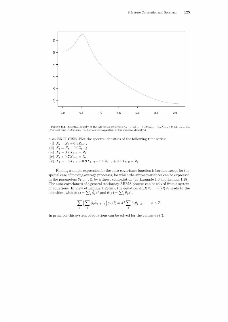
8/13/2019 van der Vaart: Time Series
http://slidepdf.com/reader/full/van-der-vaart-time-series 131/235
8.5: Auto Correlation and Spectrum 125
0.0 0.5 1.0 1.5 2.0 2.5 3.0
- 1 0
- 5
0
5
1 0
1 5
Figure 8.1. Spectral density of the AR series satisfying X t −1.5X t − 1 + 0 .9X t − 2 −0.2X t − 3 +0 .1X t − 9 = Z t .(Vertical axis in decibels , i.e. it gives the logarithm of the spectral density.)
8.23 EXERCISE. Plot the spectral densities of the following time series:(i) X t = Z t + 0 .9Z t−1;
(ii) X t = Z t −0.9Z t−1;(iii) X t −0.7X t−1 = Z t ;(iv) X t + 0 .7X t−1 = Z t ;(v) X t −1.5X t−1 + 0 .9X t−2 −0.2X t−3 + 0 .1X t−9 = Z t .
Finding a simple expression for the auto-covariance function is harder, except for thespecial case of moving average processes, for which the auto-covariances can be expressedin the parameters θ1 , . . . , θq by a direct computation (cf. Example 1.6 and Lemma 1.28).The auto-covariances of a general stationary ARMA process can be solved from a systemof equations. In view of Lemma 1.28(iii), the equation φ(B )X t = θ(B )Z t leads to theidentities, with φ(z) = j φj z j and θ(z) = j θj z j ,
l j
φj φj + l−h γ X (l) = σ2
j
θj θj + h , h Z .
In principle this system of equations can be solved for the values γ X (l).
8/13/2019 van der Vaart: Time Series
http://slidepdf.com/reader/full/van-der-vaart-time-series 132/235
126 8: ARIMA Processes
An alternative method to compute the auto-covariance function is to write X t =ψ(B )Z t for ψ = θ/φ , whence, by Lemma 1.28(iii),
γ X (h) = σ2
j
ψj ψj + h .
This requires the computation of the coefficients ψj , which can be expressed in thecoefficients of φ and θ by comparing coefficients in the power series equation φ(z)ψ(z) =
θ(z). Even in simple situations many ψj must be taken into account.
8.24 Example. For the AR(1) series X t = φX t−1 + Z t with |φ| < 1 we obtain ψ(z) =(1−φz)−1 = ∞j =0 φj z j . Therefore, γ X (h) = σ2 ∞j =0 φj φj + h = σ2φh / (1−φ2) for h ≥ 0.
8.25 EXERCISE. Find γ X (h) for the stationary ARMA(1 , 1) series X t = φX t−1 + Z t +θZ t−1 with |φ| < 1.
* 8.26 EXERCISE. Show that the auto-covariance function of a stationary ARMA processdecreases exponentially. Give an estimator of the constant in the exponent in terms of the distance of the zeros of φ to the unit circle.
A third method to express the auto-covariance function in the coefficients of thepolynomials φ and θ uses the spectral representation
γ X (h) = π
−πeihλ f X (λ) dλ =
σ2
2πi |z |=1zh−1 θ(z)θ(z−1 )
φ(z)φ(z−1 ) dz.
The second integral is a contour integral along the positively oriented unit circle in thecomplex plane. We have assumed that the coefficients of the polynomials φ and θ arereal, so that φ(z)φ(z−1 ) = φ(z)φ(z) = |φ(z)|2 for every z in the unit circle, and similarlyfor θ. The next step is to evaluate the contour integral with the help of the residuetheorem from complex function theory. † The poles of the integrand are contained in theset consisting of the zeros vi and their inverses v−1
i of φ and possibly the point 0. Theauto-covariance function can be written as a function of the residues at these points.
8.27 Example (ARMA (1, 1)) . Consider the stationary ARMA(1 , 1) series X t =φX t−1 + Z t + θZ t−1 with 0 < |φ| < 1. The corresponding function φ(z)φ(z−1) has zeros of multiplicity 1 at the points φ−1 and φ. Both points yield a pole of rst order for the inte-grand in the contour integral. The number φ−1 is outside the unit circle, so we only needto compute the residue at the second point. The function θ(z−1)/φ (z−1) = ( z + θ)/ (z−φ)is analytic on the unit disk except at the point φ and hence does not contribute other
† Remember that the residue at a point z 0 of a meromorf function f is the coefficient a − 1 in its Laurentseries representation f (z ) = Σ j a j (z − z0 ) j around z 0 . If f can be written as h (z ) / (z − z0 ) k for a function hthat is analytic on a neighbourhood of z 0 , then a − 1 can be computed as h ( k − 1) (z 0 ) / (k − 1)!. For k = 1 it isalso lim z → z 0 (z − z0 ) f (z ).
8/13/2019 van der Vaart: Time Series
http://slidepdf.com/reader/full/van-der-vaart-time-series 133/235
8.6: Existence of Causal and Invertible Solutions 127
poles, but the term zh −1 may contribute a pole at 0. For h ≥ 1 the integrand has polesat φ and φ−1 only and hence
γ X (h) = σ2 resz = φ
zh−1 (1 + θz)(1 + θz−1)(1 −φz)(1 −φz−1)
= σ2 φh (1 + θφ)(1 + θ/φ )1 −φ2 .
For h = 0 the integrand has an additional pole at z = 0 and the integral evaluates tothe sum of the residues at the two poles at z = 0 and z = φ. The rst residue is equal to
−θ/φ . Thusγ X (0) = σ2 (1 + θφ)(1 + θ/φ )
1 −φ2 − θφ
.
The values of γ X (h) for h < 0 follow by symmetry.
8.28 EXERCISE. Find the auto-covariance function for a MA( q ) process by using theresidue theorem. (This is not easier than the direct derivation, but perhaps instructive.)
We do not present an additional method to compute the partial auto-correlationfunction of an ARMA process. However, we make the important observation that for acausal AR( p) process the partial auto-correlations αX (h) of lags h > p vanish.
8.29 Theorem. For a causal AR ( p) process, the partial auto-correlations αX (h) of lags h > p are zero.
Proof. This follows by combining Lemma 2.33 and the expression for the best linearpredictor found in the preceding section.
8.6 Existence of Causal and Invertible Solutions
In practice we never observe the white noise process Z t in the denition of an ARMAprocess. The Z t are “hidden variables”, whose existence is hypothesized to explain theobserved series X t . From this point of view our earlier question of existence of a stationarysolution to the ARMA equation is perhaps not the right question, as it took the sequenceZ t as given. In this section we turn this question around and consider an ARMA( p, q )process X t as given. We shall see that there are at least 2 p+ q white noise processes Z t suchthat φ(B )X t = θ(B )Z t for certain polynomials φ and θ of degrees p and q , respectively.(These polynomials depend on the choice of Z t and hence are not necessarily the ones thatare initially given.) Thus the white noise process Z t is far from being uniquely determinedby the observed series X t . On the other hand, among the multitude of solutions, only onechoice yields a representation of X t as a stationary ARMA process that is both causaland invertible.
8/13/2019 van der Vaart: Time Series
http://slidepdf.com/reader/full/van-der-vaart-time-series 134/235
128 8: ARIMA Processes
8.30 Theorem. For every stationary ARMA process X t satisfying φ(B )X t = θ(B )Z t for polynomials φ and θ such that θ has no roots on the unit circle, there exist polynomials φ and θ of the same or smaller degrees as φ and θ that have all roots outside the unitdisc and a white noise process Z t such that φ (B )X t = θ (B )Z t , almost surely, for every t Z .
Proof. The existence of the stationary ARMA process X t and our implicit assumptionthat φ and θ are relatively prime imply that φ has no roots on the unit circle. Thusall roots of φ and θ are either inside or outside the unit circle. We shall show that wecan move the roots inside the unit circle to roots outside the unit circle by a lteringprocedure. Suppose that
φ(z) = −φ p(z −v1 ) · · ·(z −v p), θ(z) = θq(z −w1 ) · · ·(z −wq).
Consider any zero zi of φ or θ. If |zi | < 1, then we replace the term ( z −zi ) in the aboveproducts by the term (1 −z i z); otherwise we keep ( z −zi ). For zi = 0, this means thatwe drop the term z −zi = z and the degree of the polynomial decreases; otherwise, thedegree remains the same. We apply this procedure to all zeros vi and wi and denote theresulting polynomials by φ and θ . Because 0 < |zi | < 1 implies that |z−1
i | > 1, thepolynomials φ and θ have all zeros outside the unit circle. For z in a neighbourhood
of the unit circle,
θ(z)φ(z)
= θ (z)φ (z)
κ(z), κ(z) =i :|vi |< 1
1 −vi zz −vi i :|w i |< 1
z −wi
1 −wi z.
Because X t = ( θ/φ )(B )Z t and we want that X t = ( θ /φ )(B )Z t , we dene the processZ t by Z t = κ(B )Z t . This is to be understood in the sense that we expand κ(z) in itsLaurent series κ(z) = j κj z j and apply the corresponding linear lter to Z t .
By construction we now have that φ (B )X t = θ (B )Z t . If |z| = 1, then |1 −zi z| =|z −zi |. In view of the denition of κ this implies that κ(z) = 1 for every z on the unitcircle and hence Z t has spectral density
f Z (λ) = κ(e−iλ ) 2f Z (λ) = 1 · σ2
2π.
This shows that Z t is a white noise process, as desired.
As are many results in time series analysis, the preceding theorem is a result onsecond moments only. For instance, if Z t is an i.i.d. sequence, then the theorem doesnot guarantee that Z t is an i.i.d. sequence as well. Only rst and second moments arepreserved by the ltering procedure in the proof, in general. Nevertheless, the theoremis often interpreted as implying that not much is lost by assuming a-priori that φ and θhave all their roots outside the unit circle.
8/13/2019 van der Vaart: Time Series
http://slidepdf.com/reader/full/van-der-vaart-time-series 135/235
8.7: Stability 129
8.31 EXERCISE. Suppose that the time series Z t is Gaussian. Show that the series Z tconstructed in the preceding proof is Gaussian and hence i.i.d..
8.7 Stability
Let φ and θ be polynomials of degrees p ≥ 1 and q ≥ 0, with φ having no roots on theunit circle. Given initial values X 1 , . . . , X p and a process Z t , we can recursively dene asolution to the ARMA equation φ(B )X t = θ(B )Z t by
(8.1)X t = φ1 X t−1 + · · ·+ φ pX t− p + θ(B )Z t , t > p,
X t− p = φ−1 p X t −φ1X t−1 −· · ·−φ p−1X t− p+1 −θ(B )Z t , t − p < 1.
Theorem 8.8 shows that the only solution X t that is bounded in L1 is the (unique)stationary solution X t = ψ(B )Z t , ofr ψ = θ/φ . Hence the solution (8.1) can only bebounded if the initial values X 1 , . . . , X p are chosen randomly according to the stationarydistribution. In particular, the process X t obtained from deterministic initial values mustnecessarily be unbounded. The “unboundedness” refers to the process ( X t : t Z ) on thefull time scale Z .
In this section we show that in the causal situation, when φ has no zeros on the unitdisc, the process X t tends to stationarity as t → ∞, given arbitrary initial values. Hencein this case the unboundedness occurs as t → −∞. This is another reason to prefer thecase that φ has no roots on the unit disc: in this case the effect of initializing the processwears off as time goes by.
Let Z t be a given white noise process and let ( X 1 , . . . , X p) and ( X 1 , . . . , X p) betwo possible sets of initial values, consisting of random variables dened on the sameprobability space.
8.32 Theorem. Let φ and θ be polynomials such that φ has no roots on the unit disc.
Let X t and ˜X t be the ARMA processes as in dened (8.1) with initial values (X 1 , . . . , X p)and ( X 1 , . . . , X p), respectively. Then X t − X t → 0 almost surely as t → ∞.
8.33 Corollary. Let φ and θ be polynomials such that φ has no roots on the unit disc.If X t is an ARMA process with arbitrary initial values, then the vector (X t , . . . , X t + k )converges in distribution to the distribution of the stationary solution to the ARMAequation, as t → ∞, for every xed k.
Proofs. For the corollary we take ( X 1 , . . . , X p) equal to the values of the stationarysolution. Then we can conclude that the difference between X t and the stationary solutionconverges to zero almost surely and hence also in distribution.
8/13/2019 van der Vaart: Time Series
http://slidepdf.com/reader/full/van-der-vaart-time-series 136/235
130 8: ARIMA Processes
For the proof of the theorem we write the ARMA relationship in the “state spaceform”, for t > p ,
X tX t−1
...X t− p+1
=
φ1 φ2 · · · φ p−1 φ p1 0 · · · 0 0...
......
...0 0 · · · 1 0
X t−1X t−2
...X t− p
+
θ(B )Z t0...0
.
Denote this system by Y t = ΦY t−1 + B t . By some algebra it can be shown thatdet(Φ −zI ) = ( −1) pz pφ(z−1), z = 0 .
Thus the assumption that φ has no roots on the unit disc implies that the eigenvalues of Φare all inside the unit circle. In other words, the spectral radius of Φ, the maximum of themoduli of the eigenvalues, is strictly less than 1. Because the sequence Φn 1/n convergesto the spectral radius as n → ∞, we can conclude that Φn 1/n is strictly less than 1for all sufficiently large n , and hence Φn → 0 as n → ∞. (In fact, if Φn 0 : = c < 1,then Φkn 0 ≤ ck for every natural number k and hence Φn ≤ Cc n/n 0 for every n,for C = max 0≤j ≤n 0 Φj , and the convergence to zero is exponentially fast.)
If Y t relates to X t as Y t relates to X t , then Y t − Y t = Φ t− p(Y p − Y p) → 0 almostsurely as t → ∞.8.34 EXERCISE. Suppose that φ(z) has no zeros on the unit circle and at least onezero inside the unit circle. Show that there exist initial values ( X 1 , . . . , X p) such that theresulting process X t is not bounded in probability as t → ∞. [Let X t be the stationarysolution and let X t be the solution given initial values ( X 1 , . . . , X p). Then, with notationas in the preceding proof, Y t − Y t = Φ t− p(Y p − Y p). Choose an appropriate deterministicvector for Y p − Y p.]
8.35 EXERCISE. Simulate a series of length 200 of the ARMA process satisfying X t −1.3X t−1 +0 .7X t−2 = Z t +0 .7Z t−1. Plot the sample path, and the sample auto-correlationand sample partial auto-correlation functions. Vary the distribution of the innovationsand simulate both stationary and nonstaionary versions of the process.
8.8 ARIMA Processes
In Chapter 1 differencing was introduced as a method to transform a nonstationary timeseries into a stationary one. This method is particularly attractive in combination withARMA modelling: in the notation of the present chapter the differencing lters can bewritten as
X t = (1 −B )X t , d X t = (1 −B )d X t , k X t = (1 −B k )X t .

8/13/2019 van der Vaart: Time Series
http://slidepdf.com/reader/full/van-der-vaart-time-series 137/235
8.9: VARMA Processes 131
Thus the differencing lters , d and k correspond to applying the operator η(B ) forthe polynomials η(z) = 1 −z, η(z) = (1 −z)d and η(z) = (1 −zk ), respectively. Thesepolynomials have in common that all their roots are on the complex unit circle. Thusthey were “forbidden” polynomials in our preceding discussion of ARMA processes.
By Theorem 8.10, for the three given polynomials η the series Y t = η(B )X t cannotbe a stationary ARMA process relative to polynomials without zeros on the unit circleif X t is a stationary process. On the other hand, the series Y t = η(B )X t can well bea stationary ARMA process if X t is a non-stationary time series. Thus we can use
polynomials with roots on the unit circle to extend the domain of ARMA modelling tononstationary time series.
8.36 Denition. A time series X t is an ARIMA( p, d, q ) process if d X t is a stationary ARMA ( p, q ) process.
In other words, the time series X t is an ARIMA( p, d, q ) process if there exist poly-nomials φ and θ of degrees p and q and a white noise series Z t such that the timeseries d X t is stationary and φ(B ) d X t = θ(B )Z t almost surely. The additional “I”in ARIMA is for “integrated”. If we view taking differences d as differentiating, thenthe denition requires that a derivative of X t is a stationary ARMA process, whence X titself is an “integrated ARMA process”.
The following denition goes a step further.
8.37 Denition. A time series X t is a SARIMA( p, d, q )(P,D,Q,per ) process if there exist polynomials φ, θ, Φ and Θ of degrees p, q , P and Q and a white noise series Z t such that the time series D
perd X t is stationary and Φ(B per )φ(B ) D
perd X t =
Θ(B per )θ(B )Z t almost surely.
The “S” in SARIMA is short for “seasonal”. The idea of a seasonal model is thatwe might only want to use certain powers B per of the backshift operator in our model,because the series is thought to have a certain period. Including the terms Φ( B per ) andΘ(B per ) does not make the model more general (as these terms could be subsumed inφ(B ) and θ(B )), but reects our a-priori idea that certain coefficients in the polynomialsare zero. This a-priori knowledge will be important when estimating the coefficients froman observed time series.
Modelling an observed time series by an ARIMA, or SARIMA, model has becomepopular through an inuential book by Box and Jenkins. The unied ltering paradigmof a “Box-Jenkins analysis” is indeed attractive. The popularity is probably also due tothe compelling manner in which Box and Jenkins explain the reader how he or she mustset up the analysis, going through a xed number of steps. They thus provide the data-analyst with a clear algorithm to carry out an analysis that is intrinsically difficult. It isobvious that the results of such an analysis will not always be good, but an alternativeis less obvious.

8/13/2019 van der Vaart: Time Series
http://slidepdf.com/reader/full/van-der-vaart-time-series 138/235

8/13/2019 van der Vaart: Time Series
http://slidepdf.com/reader/full/van-der-vaart-time-series 139/235
8.10: ARMA-X Processes 133
rule, which expresses the solution of a system of linear equations in determinants, showsthat the entries of the inverse matrices Φ( z)−1 and Θ( z)−1 are quotients of polynomials.The denominators are the determinants det Φ( z) and det Θ( z) and hence are nonzero ina neighbourhood of the unit circle. These matrices may thus be expanded (entrywise) inLaurent series’
Φ(z)−1 =∞
j = −∞(Φj )k,l z j
k,l =1 ,...,d=
∞
j = −∞Φj z j ,
where the Φ j are matrices such that ∞j = −∞ Φj < ∞, and similarly for Θ( z)−1 . Thisallows the back-shift calculus that underlies the proof of Theorem 8.8. For instance, thematrix-valued function Ψ = Φ −1Θ is well-dened on the unit circle, and can be expandedas Ψ(z) = ∞j = −∞ Ψj z j for matrices Ψ j with ∞j = −∞ Ψj < ∞. The process Ψ( B )Z tis the unique solution to the VARMA-equation.
* 8.10 ARMA-X Processes
The (V)ARMA-relation models a time series as an autonomous process, whose evolution
is partially explained by its own past (or the past of the other coordinates in the vector-valued situation). It is often of interest to include additional explanatory variables intothe model. The natural choice of including time-dependent, vector-valued variables W tlinearly yields the ARMA-X model
X t = Φ1 X t−1 + Φ 2X t−2 + · · ·+ Φ pX t− p + Z t + Θ 1Z t−1 + · · ·+ Θ qZ t−q + β T W t .
8/13/2019 van der Vaart: Time Series
http://slidepdf.com/reader/full/van-der-vaart-time-series 140/235
9GARCH Processes
White noise processes are basic building blocks for time series models, but can also be of interest on their own. A sequence of i.i.d. variables is white noise sequence that is not of great interest as a time series. On the other hand, many nancial time series appear tobe realizations of white noise series that have interesting time structure. This is possible,because the white noise property only concerns the second moments of the process,so that the variables of a white noise process may possess many types of dependence.GARCH processes are white noises that have been found useful for modelling nancialtime series.
Figure 9.1 shows a realization of a GARCH process. The striking feature are the“bursts of activity”, which alternate with quiet periods of the series. The frequencyof the movements of the series appears to be constant over time, but their amplitudechanges, alternating between “volatile” periods (large amplitude) and quiet periods. Thisphenomenon is referred to as volatility clustering . A look at the auto-correlation functionof the realization, Figure 9.2, shows that the alternations are not reected in the secondmoments of the series: the series can be modelled as white noise, at least in the sensethat the correlations are zero.
Recall that a white noise series is any mean-zero stationary time series whose auto-covariances at nonzero lags vanish. We shall speak of a heteroscedastic white noise if the
auto-covariances at nonzero lags vanish, but the variances are possibly time-dependent.A related concept is that of a martingale difference series. Recall that a ltration F t is anondecreasing collection of σ-elds · ·· F −1 F 0 F 1 ·· ·. A martingale difference series relative to the ltration F t is a time series X t such that X t is F t -measurable andE( X t |F t−1) = 0, almost surely, for every t. (The latter includes the assumption thatE|X t | < ∞, so that the conditional expectation is well dened.)
Any martingale difference series X t with nite second moments is a (possibly het-eroscedastic) white noise series. Indeed, the equality E( X t |F t−1) = 0 is equivalent toX t being orthogonal to all random variables Y F t−1 , and this includes the variablesX s F s F t−1 , for every s < t , so that E X t X s = 0 for every s < t . The converseis false: not every white noise is a martingale difference series (relative to a natural l-
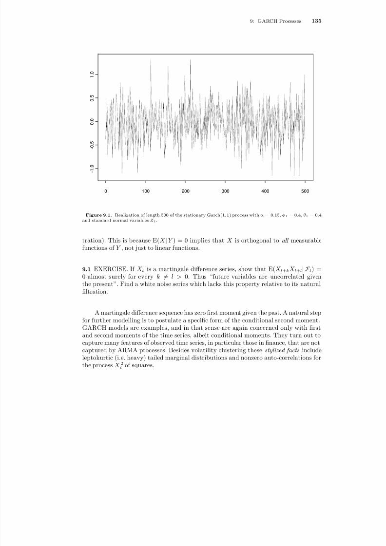
8/13/2019 van der Vaart: Time Series
http://slidepdf.com/reader/full/van-der-vaart-time-series 141/235
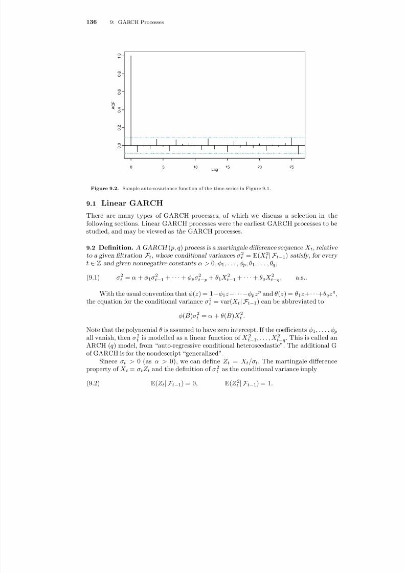
8/13/2019 van der Vaart: Time Series
http://slidepdf.com/reader/full/van-der-vaart-time-series 142/235
136 9: GARCH Processes
0 5 10 15 20 25
0 . 0
0 . 2
0 . 4
0 . 6
0 . 8
1 . 0
Lag
A C F
Figure 9.2. Sample auto-covariance function of the time series in Figure 9.1.
9.1 Linear GARCH
There are many types of GARCH processes, of which we discuss a selection in thefollowing sections. Linear GARCH processes were the earliest GARCH processes to bestudied, and may be viewed as the GARCH processes.
9.2 Denition. A GARCH ( p, q ) process is a martingale difference sequence X t , relative to a given ltration F t , whose conditional variances σ2
t = E( X 2t |F t−1) satisfy, for every t Z and given nonnegative constants α > 0, φ1 , . . . , φ p, θ1 , . . . , θq ,
(9.1) σ2t = α + φ1σ2
t−1 + · · ·+ φ pσ2t− p + θ1X 2t−1 + · · ·+ θqX 2t−q , a.s..
With the usual convention that φ(z) = 1
−φ1z
−···−φ pz p and θ(z) = θ1z+
· · ·+ θqzq ,
the equation for the conditional variance σ2t = var( X t |F t−1) can be abbreviated to
φ(B )σ2t = α + θ(B )X 2t .
Note that the polynomial θ is assumed to have zero intercept. If the coefficients φ1 , . . . , φ pall vanish, then σ2
t is modelled as a linear function of X 2t−1 , . . . , X 2t−q . This is called anARCH ( q ) model, from “auto-regressive conditional heteroscedastic”. The additional Gof GARCH is for the nondescript “generalized”.
Sinece σt > 0 (as α > 0), we can dene Z t = X t /σ t . The martingale differenceproperty of X t = σt Z t and the denition of σ2
t as the conditional variance imply
(9.2) E( Z t |F t−1) = 0 , E(Z 2t |F t−1) = 1 .

8/13/2019 van der Vaart: Time Series
http://slidepdf.com/reader/full/van-der-vaart-time-series 143/235
8/13/2019 van der Vaart: Time Series
http://slidepdf.com/reader/full/van-der-vaart-time-series 144/235
138 9: GARCH Processes
volatility with periods of low volatility. This volatility clustering is one of the stylized facts of nancial time series. The phrase “stylized fact” is used for salient propertiesthat seem to be shared by many nancial time series, although “fact” is not to be takenliterally.
A second stylized fact are the leptokurtic tails of the marginal distribution of atypical nancial time series. A distribution on R is called leptokurtic if it has fat tails,for instance fatter than normal tails. A quantitative measure of “fatness” of the tailsof the distribution of a random variable X is the kurtosis dened as κ4(X ) = E( X
−EX )4 / (var X )2 . If X t = σt Z t , where σt is F t−1-measurable and Z t is independent of F t−1 with mean zero and variance 1, then
EX 4t = E σ4t EZ 4t = κ4(Z t )E E(X 2t |F t−1) 2
≥κ4(Z t )(E σ2t )2 = κ4(Z t )(E X 2t )
2 .
Dividing the left and right sides by (E X 2t )2 , we see that κ4 (X t ) ≥ κ4(Z t ). The differencecan be substantial if the variance of the random variable E( X 2t |F t−1) is large. In fact,taking the difference of the left and right sides of the preceding display yields
κ4(X t ) = κ4(Z t ) 1 + var E( X 2t |F t−1)
(EX 2t )2 .
It follows that the GARCH structure is also able to capture some of the observed lep-tokurtosis of nancial time series.
The kurtosis of a normal variable is equal to 3. Thus for a Gaussian driving processZ t , the kurtosis of the observed series X t is always bigger than 3. It has been observedthat this usually does not go far enough in explaining “excess kurtosis” over the normaldistribution. The use of one of Student’s t-distributions can often improve the t of aGARCH process substantially.
If we substitute σ2t = X 2t −W t in (9.1), then we nd after rearranging the terms,
(9.3) X 2t = α + ( φ1 + θ1 )X 2t−1 + · · ·+ ( φr + θr )X 2t−r
+ W t −φ1W t−1 − · · ·−φ pW t− p ,
where r = p q and the sequences φ1 , . . . , φ p or θ1 , . . . , θq are padded with zeros toincrease their lengths to r , if necessary. We can abbreviate this to
(φ −θ)(B )X 2t = α + φ(B )W t , W t = X
2t −E( X
2t |F t−1).
This is the characterizing equation for an ARMA( r, r ) process X 2t relative to the noiseprocess W t . The variable W t = X 2t −σ2
t is the prediction error when predicting X 2t byits conditional expectation σ2
t = E( X 2t |F t−1) and hence W t is orthogonal to F t−1 . ThusW t is a martingale difference series and a-fortiori a white noise sequence if its secondmoments exist and are independent of t.
Under these conditions the time series of squares X 2t is an ARMA process in thesense of Denition 8.4. This observation is useful to compute certain characteristics of the process. However, the variables W t in equation (9.3) are dened in terms of of theprocess X t (their squares and conditional variances) and therefore do not have a simpleinterpretation as a noise process that drives the process X 2t . This circularity makes that

8/13/2019 van der Vaart: Time Series
http://slidepdf.com/reader/full/van-der-vaart-time-series 145/235
9.1: Linear GARCH 139
one should not apply results on ARMA processes unthinkingly to the process X 2t . Forinstance, equation (9.3) seems to have little use for proving existence of solutions to theGARCH equation.
* 9.4 EXERCISE. Suppose that X t and W t are martingale diffference series’ relative to agiven ltration such that φ(B )X 2t = θ(B )W t for polynomials φ and θ of degrees p andq . Show that X t is a GARCH process. Does strict stationarity of the time series X 2t orW t imply strict stationarity of the time series X t ?
9.5 EXERCISE. Write σ2t as the solution to an ARMA( p q, q −1) equation by substi-
tuting X 2t = σ2t + W t in (9.3).
9.1.1 Autocovariances of Squares
Even though the autocorrelation function of a GARCH process vanishes (except at lagzero), the variables are not independent. One way of seeing this is to consider the auto-correlations of the squares X 2t of the time series. Independence of the X t would implyindependence of the X 2t , and hence a zero autocorrelation function. However, in viewof (9.3) the squares form an ARMA process, whence their autocorrelations are nonzero.
The auto-correlations of the squares of nancial time series are typically observed to bepositive at all lags, another stylized fact of such series.
The auto-correlation function of the squares of a GARCH series will exist underappropriate additional conditions on the coefficients and the driving noise process Z t .The ARMA relation (9.3) for the square process X 2t may be used to derive this function,from the formulas for the auto-correlation function of an ARMA process. Here we mustnot forget that the process W t in (9.3) is dened through X t and hence its variancedepends on the parameters in the GARCH relation.
Actually, equation (9.3) is an ARMA equation “with intercept α”. Provided thatφ(1) = 0, we can rewrite it as φ(B ) X 2t −α/φ (1) = φ(B ), which shows that the timeseries X 2t is an ARMA proces plus α/φ (1). The autocorrelations are of course independentof this shift.
9.6 Example (GARCH (1, 1)) . The conditional variances of a GARCH(1,1) processsatisfy σ2
t = α + φσ2t−1 + θX 2t−1 . If we assume the process X t to be stationary, then
Eσ2t = E X 2t is independent of t. Taking the expectation across the GARCH equation
and rearranging then immediately gives
Eσ2t = E X 2t =
α1 −φ −θ
.
To compute the auto-correlation function of the time series of squares X 2t , we employ(9.3), which reveals this process as an ARMA(1,1) process with the auto-regressive andmoving average polynomials given as 1 −(φ+ θ)z and 1−φz, respectively. The calculations

8/13/2019 van der Vaart: Time Series
http://slidepdf.com/reader/full/van-der-vaart-time-series 146/235
140 9: GARCH Processes
in Example 8.27 yield that
γ X 2 (h) = τ 2 (φ + θ)h (1 −φ(φ + θ))(1 −φ/ (φ + θ))1 −(φ + θ)2 , h > 0,
γ X 2 (0) = τ 2(1 −φ(φ + θ))(1 −φ/ (φ + θ))
1 −(φ + θ)2 + φφ + θ
.
Here τ 2 is the variance of the process W t = X 2t −E(X 2t |F t−1), which is also dependenton the parameters θ and φ. By squaring the GARCH equation we nd
σ4t = α2 + φ2 σ4
t−1 + θ2X 4t−1 + 2 αφσ 2t−1 + 2 αθX 2
t−1 + 2 φθσ2t−1 X 2t−1 .
If Z t is independent of F t−1 , then E σ2t X 2t = E σ4
t and EX 4t = κ4(Z t )Eσ4t . If we assume,
moreover, that the moments exists and are independent of t, then we can take theexpectation across the preceding display and rearrange to nd that
Eσ4t (1 −φ2 −2φθ −κ4(Z )θ2 ) = α2 + (2 αφ + 2 αθ)Eσ2
t .
Together with the formulas obtained previously, this gives the variance of W t , sinceEW t = 0 and E W 2t = E X 4t −Eσ4
t , by Pythagoras’ identity for projections.
9.7 EXERCISE. Find the auto-covariance function of the process σ2t for a GARCH(1 , 1)
process.
9.8 EXERCISE. Find an expression for the kurtosis of the marginal distribution in a sta-tionary GARCH(1 , 1) process as in the preceding example. Can this be made arbitrarilylarge?
9.1.2 Stationary SolutionsBecause the GARCH relation is recursive and the variables X t enter it both explicitly andimplicitly (through their conditional variances) existence of stationary GARCH processesis far from obvious. In this section we show that a (strictly) stationary solution existsonly for certain parameter values φ1 , . . . , φ p, θ1 . . . , θq , and if it exists, then it is unique.A bit surprisingly, a strictly stationary solution exists for a larger set of parameter valuesthan a second order stationary solution.
We start with investigating second order stationary solutions. Substituting X t =σt Z t in the GARCH relation (9.1), we obtain
(9.4) σ2t = α + ( φ1 + θ1Z 2t−1)σ2
t−1 + · · ·+ ( φr + θr Z 2t−r )σ2t−r .
This exhibits the process σ2t as an auto-regressive process “with random coefficients”
(the variables φi + θi Z 2t−i ) and “deterministic innovations” (the constant α). We shallconstruct and study the process σ2
t by considering this equation in a state space rep-resentation, with state vectors ( σ2
t−1 , . . . , σ 2t−r ). Given the process σ2
t , we next obtain aGARCH process as X t = σt Z t .
In the following theorem we consider given a martingale difference sequence Z tsatisfying (9.2), dened on a xed probability space. A stationary GARCH process existsif and only if j (φj + θj ) < 1.
8/13/2019 van der Vaart: Time Series
http://slidepdf.com/reader/full/van-der-vaart-time-series 147/235
9.1: Linear GARCH 141
9.9 Theorem. Let α > 0, let φ1 , . . . , φ p , θ1 , . . . , θq be nonnegative numbers, and let Z tbe a martingale difference sequence satisfying (9.2) relative to an arbitrary ltration F t .(i) There exists a stationary GARCH process X t such that X t = σt Z t , where σ2
t =E( X 2t |F t−1), if and only if j (φj + θj ) < 1.
(ii) This process is unique among the GARCH processes X t with X t = σt Z t that are bounded in L2 .
(iii) This process satises σ(X t , X t−1 , . . .) = σ(Z t , Z t−1 , . . .) for every t, and σ2t =
E( X 2t
|F t−1) is σ(X t−1 , X t−2 , . . .)-measurable.
Proof. The recursion equation (9.4) can be written in matrix form as
σ2t
σ2t−1...
σ2t−r +1
=
φ1 + θ1Z 2t−1 · · · φr −1 + θr −1Z 2t−r +1 φr + θr Z 2t−r1 · · · 0 0...
. . . ...
...0 · · · 1 0
σ2t−1
σ2t−2...
σ2t−r
+
α0...0
.
Writing this system as Y t = At Y t−1 + b, and iterating we nd, for every n ≥ 1,
(9.5) Y t = b+ At b + At At−1b + · · ·+ At At−1 · · ·At−n +1 b + At At−1 · · ·At−n Y t−n −1 .
If the last term on the right tends to zero as n → ∞, then this gives
(9.6)
Y t =
b+
∞
j =1 At At−1 · · ·At−j +1 b.
We shall prove that this representation is indeed valid for the process Y t correspondingto a GARCH process that is bounded in L2 . Because the right side of the display is afunction of the Z t only, the uniqueness (ii) of such a GARCH process for a given processZ t is then clear. To prove existence, as in (i), we shall reverse this argument: we useequation (9.6) to dene a process Y t , and next dene processes σt and X t as functionsof Y t and Z t .
We start by studying the random matrix products A t At−1 · · ·At−n .The expectation A = E At of a single matrix is obtained by replacing the variables
Z 2s in the denition of A t by their expectation 1. The expectation of the product turnsout to be the product of the expectations E At At−1 · · ·At−n = An +1 . To see this, writeAt = Φ + q
j =1 θj Z 2t j L j , for Lj the matrix with rst row the j th unit vector and 0selsewhere. Then L1L j = Lj and Li L j = 0 for every j ≥ 1 and i ≥ 2, and hencethe product At At−1 · · ·At−n can be written as a linear combination of deterministicmatrices with random coefficients of the type Z 2t 1 · · ·Z 2t k = 1, for t1 < t 2 < · · · < t k .Noting that Z t = X t /σ t is F t -measurable and E( Z 2t |F t−1) = 1 for every t, we can usethe towering property of conditional expectations to see that E Z 2t 1 · · ·Z 2t k = 1, for everyt1 < t 2 < · · · < t k . Hence the expected value E At At−1 · · ·At−n can also be computed byreplacing every Z 2s by its expectation 1, yielding An +1 as claimed.
The characteristic polynomial of the matrix A can (with some effort) be seen to beequal to
det( A −zI ) = ( −1)r zr −r
j =1
(φj + θj )zr −j .
8/13/2019 van der Vaart: Time Series
http://slidepdf.com/reader/full/van-der-vaart-time-series 148/235
142 9: GARCH Processes
If j (φj + θj ) < 1, then the polynomial on the right has all its roots inside the unit circle.(See Exercise 9.10, with z replaced by 1 /z .) The spectral radius (the maximum of themoduli of the eigenvalues) of the operator A is then strictly smaller than 1. This impliesthat An 1/n is smaller than 1 for all sufficiently large n and hence ∞n =0 An < ∞.
Combining the results of the last two paragraphs we see that E At At−1 · · ·At−n =An +1 → 0 as n → ∞ if j (φj + θj ) < 1. Because the matrices A t possess nonnegativeentries, this implies that the sequence A t At−1 · · ·At−n converges to zero in probability.If X t is a GARCH process that is bounded in L2 , then, in view of its denition, the
corresponding process Y t is bounded in L1 . In that case At At−1 · · ·At−n Y t−n −1 → 0in probability as n → ∞, and hence Y t satises (9.6). This concludes the proof of theuniqueness (ii).
Under the assumption that j (φj + θj ) < 1, the series on the right side of (9.6)converges in L1 . Thus we can use this equation to dene a process Y t from the givenmartingale difference series Z t . Simple algebra on the innite series shows that Y t =At Y t−1 + b for every t. Clearly the coordinates of Y t are nonnegative, whence we candene processes σt and X t by
σt = Y t, 1 , X t = σt Z t .
Because σt is σ(Z t−1 , Z t−2 , . . .) F t−1-measurable, we have that E( X t |F t−1) =σt E(Z t
|F t−1) = 0 and E( X 2t
|F t−1) = σ2
t E( Z 2t
|F t−1) = σ2
t . Furthermore, the process
σ2t satises the GARCH relation (9.1). Indeed, the rst row of the matrix equationY t = A t Y t−1 + b expresses σ2
t into σ2t−1 and Y t−1,2 , . . . , Y t−1,r , and the other rows per-
mit to reexpress the variable Y t−1,k for k > 1 as σ2t−k by recursive use of the relations
Y t,k = Y t−1,k −1 , and the denitions Y t−k, 1 = σ2t−k . This concludes the proof that there
exists a stationary solution as soon as j (φj + θj ) < 1.To see that the latter condition is necessary, we return to equation (9.5). If X t is a
stationary solution, then its conditional variance process σ2t is integrable, and hence so is
the process Y t in (9.5). Taking the expectation of the left and right sides of this equationfor t = 0 and remembering that all terms are nonnegative, we see that
nj =0 Aj b ≤EY 0 ,
for every n. This implies that An b → 0 as n → ∞, or, equivalently An e1 → 0, where eiis the ith unit vector. In view of the denition of A we see, recursively, that
An er = An −1(φr + θr )e1
→ 0,
An er −1 = An −1 (φr −1 + θr −1)e1 + er → 0,...
An e2 = An −1 (φ2 + θ2)e1 + e3 → 0.
Therefore, the sequence An converges to zero. This can only happen if none of its eigen-values is on or outside the unit disc. This was seen to be case only if
rj =1 (φj + θj ) < 1.
This concludes the proof of (i) and (ii). For the proof of (iii) we rst note that thematrices At , and hence the variables Y t , are measurable functions of ( Z t−1 , Z t−2, . . .).In particular, the variable σ2
t , which is the rst coordinate of Y t , is σ(Z t−1 , Z t−2 , . . .)-measurable, so that the second assertion of (iii) follows from the rst.

8/13/2019 van der Vaart: Time Series
http://slidepdf.com/reader/full/van-der-vaart-time-series 149/235
9.1: Linear GARCH 143
Because the variable X t = σt Z t is a measurable transformation of ( Z t , Z t−1, . . .),it follows that σ(X t , X t−1 , . . .) σ(Z t , Z t−1 , . . .). To prove the converse, we note thatthe process W t = X 2t − σ2
t is bounded in L1 and satises the ARMA relation ( φ −θ)(B )X 2t = α + φ(B )W t , as in (9.3). Because φ has no roots on the unit disc, this relationis invertible, whence W t = (1 /φ )(B ) (φ −θ)(B )X 2t −α is a measurable transformationof X 2t , X 2t−1 , . . .. Therefore σ2
t = W t + X 2t and hence Z t = X t /σ t is σ(X t , X t−1 , . . .)-measurable.
9.10 EXERCISE. If p1 , . . . , pr are nonnegative real numbers, then the polynomial p(z) =1 −
rj =1 pj z j possesses no roots on the unit disc if and only if p(1) > 0. [Use that
p(0) = 1 > 0; furthermore, use the triangle inequality.]
Theorem 9.9’s condition j (φj + θj ) < 1 is necessary for existence of a GARCHprocess with bounded second moments, but stronger than necessary if we are interestedin a strictly stationary solution to the GARCH equations with possibly innite secondmoments. We can see this from the proof, where the GARCH process is dened fromthe series in (9.6). If this series converges in an appropriate sense, then a strictly sta-tionary GARCH process exists. The series involves products of random matrices A t ; itsconvergence depends on the value of their top Lyapounov exponent , dened by
γ = inf n N
1n
Elog A−1A−2 · · ·A−n .
Here · may be any matrix norm (all matrix norms being equivalent). If the processZ t is ergodic, for instance i.i.d., then we can apply Kingman’s subergodic theorem (e.g.Dudley (1987, Theorem 10.7.1)) to the process log A−1A−2 · · ·A−n to see that
1
n log A−1A−2
· · ·A−n
→ γ , a.s..
This implies that the sequence of matrices A−1A−2 · · ·A−n converges to zero almostsurely as soon as γ < 0. The convergence is then exponentially fast and the series in(9.6) will converge.
Thus sufficient conditions for the existence of strictly stationary solutions to theGARCH equations can be given in terms of the top Lyapounov exponent of the randommatrices A t . This exponent is in general difficult to compute explicitly, but it can easilybe estimated numerically for a given sequence Z t .
To obtain conditions that are both sufficient and necessary the preceding proof mustbe adapted somewhat. The following theorem is in terms of the top Lyapounov exponent

8/13/2019 van der Vaart: Time Series
http://slidepdf.com/reader/full/van-der-vaart-time-series 150/235

8/13/2019 van der Vaart: Time Series
http://slidepdf.com/reader/full/van-der-vaart-time-series 151/235
9.1: Linear GARCH 145
The matrix B obtained by replacing the variables Z t−1 and the numbers θj in thematrix At by zero is bounded above by At in a coordinatewise sense. By the nonnegativityof the entries this implies that Bn ≤ A0 A−1 · · ·A−n +1 and hence Bn → 0. This canhappen only if all eigenvalues of B are inside the unit circle. Indeed, if z is an eigenvalueof B with |z| ≥ 1 and c = 0 a corresponding eigenvector, then Bn c = zn c does notconverge to zero. Now
det( B −zI ) = ( −z) p+ q−1φ(1/z ).Thus z is a zero of φ if and only if z−1 is an eigenvalue of B . We conclude that φ has nozeros on the unit disc.
Finally, we show the necessity of the top Lyapounov exponent being negative. If there exists a strictly stationary solution to the GARCH equations, then, by (9.5) and thenonnegativity of the coefficients,
nj =1 A0A−1 · · ·A−n +1 b ≤ Y 0 for every n, and hence
A0 A−1 · · ·A−n +1 b → 0 as n → ∞, almost surely. By the form of b this is equivalentto A0 A−1 · · ·A−n +1 e1 → 0. Using the structure of the matrices At we next see thatA0 A−1 · · ·A−n +1 → 0 in probability as n → ∞, by an argument similar as in theproof of Theorem 9.9. Because the matrices At are independent and the event whereA0 A−1 · · ·A−n +1 → 0 is a tail event, this event must have probability one. It can beshown that this is possible only if the top Lyapounov exponent of the matrices At isnegative. ‡
9.12 Lemma. Let φ be a polynomial without roots on the unit disc and let X t be a time series that is bounded in probability. If Z t = φ(B )X t for every t, then X t is σ(Z t , Z t−1 , . . .)-measurable.
Proof. Because φ(0) = 0 by assumption, we can assume without loss of generalitythat φ possesses intercept 1. If φ is of degree 0, then X t = Z t for every t and theassertion is certainly true. We next proceed by induction on the degree of φ. If φ is of degree p ≥ 1, then we can write it as φ(z) = (1 − φz)φ p−1 (z) for a polynomial φ p−1of degree p −1 and a complex number φ with |φ| < 1. The series Y t = (1 −φB )X t isbounded in probability and φ p−1(B )Y t = Z t , whence Y t is σ(Z t , Z t−1 , . . .)-measurable,by the induction hypothesis. By iterating the relation X t = φX t−1 + Y t , we nd thatX t = φn X t−n + n −1
j =0 φj Y t−j . Because the sequence X t is uniformly tight and φn → 0,the sequence φn X t−n converges to zero in probability. Hence X t is the limit in probabilityof a sequence that is σ(Y t , Y t
−1 , . . .)-measurable and hence is σ(Z t , Z t
−1 , . . .)-measurable.
This implies the result.
** 9.13 EXERCISE. In the preceding lemma the function ψ(z) = 1 /φ (z) possesses a powerseries representation ψ(z) = ∞j =0 ψj z j on a neighbourhood of the unit disc. Is it trueunder the conditions of the lemma that X t = ∞j =0 ψj Z t−j , where the series converges(at least) in probability?
9.14 Example. For the GARCH(1 , 1) process the random matrices At given by (9.7)reduce to the random variables φ1 + θ1Z 2t−1 . The top Lyapounov exponent of these ran-dom (1 ×1) matrices is equal to E log( φ1 + θ1Z 2t ). This number can be written as an
‡ See Bougerol (), Lemma ?.

8/13/2019 van der Vaart: Time Series
http://slidepdf.com/reader/full/van-der-vaart-time-series 152/235

8/13/2019 van der Vaart: Time Series
http://slidepdf.com/reader/full/van-der-vaart-time-series 153/235
9.1: Linear GARCH 147
(i) If j (φj + θj ) < 1, then the difference X t − X t of any two solutions X t = σt Z t and X t = σt Z t of the GARCH equations that are square-integrable converges to zero inL2 as t → ∞.(ii) If the top Lyapounov exponent of the matrices At in (9.7) is negative, then the difference X t − X t of any two solutions X t = σt Z t and X t = σt Z t of the GARCH equations converges to zero in probability as t → ∞.
Proof. From the two given GARCH processes X t and X t dene processes Y t and Y t asindicated preceding the statement of Theorem 9.11. These processes satisfy (9.5) for thematrices A t given in (9.7). Choosing n = t −1 and taking differences we see that
Y t − Y t = At At−1 · · ·A1 (Y 0 − Y 0).
If the top Lyapounov exponent of the matrices At is negative, then the norm of theright side can be bounded, almost surely for sufficiently large t , by by eγ t Y 0 − Y 0 forsome number γ < 0. This follows from the subergodic theorem, as before (even thoughthis time the matrix product grows on its left side). This converges to zero as t → ∞,implying that σt − σt → 0 almost surely as t → ∞. This in turn implies (ii).
Under the condition of (i), the spectral radius of the matrix A = E At is strictlysmaller than 1 and hence An → 0. By the nonnegativity of the entries of the matricesAt the absolute values of the coordinates of the vectors Y t − Y t are bounded above by
the coordinates of the vector A t At−1 · · ·A1W 0 , for W 0 the vector obtained by replacingthe coordinates of Y 0 − Y 0 by their absolute values. By the independence of the matricesAt and vector W 0 , the expectation of At At−1 · · ·A1 W 0 is bounded by At EW 0 , whichconverges to zero. Because σ2
t = Y t, 1 and X t = σt Z t , this implies that, as t → ∞,E|X 2t − X 2t | = E |σ2
t − σ2t |Z 2t = E |σ2
t − σ2t | → 0.
For the stationary solution X t the sequence ( X 2t ) is uniformly integrable, because thevariables X 2t possess a xed marginal distribution with nite second moment. By thepreceding display this is then also true for X t , and hence also for a general X t . Thesequence X t − X t is then uniformly square-integrable as well. Combining this with thefact that X t − X t → 0 in probability, we see that X t − X t converges to zero in secondmean.
The preceding theorem may seem at odds with a common interpretation of a sta-tionary and stability condition as a condition for “persistence”. The condition for L2-stationarity of a GARCH process is stronger than the condition for strict stationarity,so that it appears as if we have found two different conditions for persistence. Whenevera strictly stationary solution exists, the inuence of initial values wears off as time goesto innity, and hence the initial values are not persistent. This is true independently of the validity of the condition j (φj + θj ) < 1 for L2-stationarity. However, the lattercondition, if it holds, does ensure that the process approaches stationarity in the strongerL2-sense.
The condition j (φj + θj ) < 1 is necessary for the strictly stationary solution to havenite second moments. By an appropriate initialization we can ensure that a GARCH

8/13/2019 van der Vaart: Time Series
http://slidepdf.com/reader/full/van-der-vaart-time-series 154/235
148 9: GARCH Processes
process has nite second moments for every t , even if this condition fails. (It will thennot be stationary.) However, in this case the variances E X 2t must diverge to innity ast → ∞. This follows by a Fatou type argument, because the process will approach thestrictly stationary solution and this has innite variance.
The case that j (φi + θj ) = 1 is often viewed as having particular interest and isreferred to as integrated GARCH or IGARCH. Many nancial time series yield GARCHts that are close to IGARCH.
9.16 EXERCISE. Suppose that the time series X t is strictly stationary with innitesecond moments and X t − X t → 0 in probability as t → ∞. Show that E X 2t → ∞.
9.1.4 Prediction
As it is a martingale difference process, a GARCH process does not allow nontriv-ial predictions of its mean values. However, it is of interest to predict the condi-tional variances σ2
t , or equivalently the process of squares X 2t . Predictions based onthe innite past F t can be obtained using the auto-regressive representation fromthe proofs of Theorems 9.11 and 9.11. Let At be the matrix given in (9.7) and letY t = ( σ2
t , . . . , σ2t− p+1 , X 2t−1 , . . . , X 2t−q+1 )T , so that Y t = At Y t−1 + b for every t. The vector
Y t−1 is F t−2-measurable, and the matrix At depends on Z t−1 only, with A = E( At |F t−2)
independent of t . It follows thatE( Y t |F t−2) = E( At |F t−2)Y t−1 + b = AY t−1 + b.
By iterating this equation we nd that, for h > 1,
E( Y t |F t−h ) = Ah −1Y t−h +1 +h−2
j =0
Aj b.
As σ2t is the rst coordinate of Y t , this equation gives in particular the predictions for
the volatility, based on the innite past. If j (φj + θj ) < 1, then the spectral radius of the matrix A is strictly smaller than 1, and both terms on the right converge to zero atan exponential rate, as h → ∞. In this case the potential of predicting the conditional
variance process is limited to the very near future. The case that j (φj + θj ) ≥ 1 ismore interesting, as is illustrated by the following example.
9.17 Example (GARCH(1,1)) . For a GARCH(1 , 1) process the vector Y t is equal to σ2t
and the matrix A reduces to the number φ1 + θ1 . The general equation can be rewrittenin the form
(9.8) E(X 2t + h |F t ) = E( σ2t + h |F t ) = ( φ1 + θ1)h−1 σ2
t +1 + αh−2
j =0(φ1 + θ1 )j .
For φ1 + θ1 < 1 the rst term on the far right converges to zero as h → ∞, indicatingthat information at the present time t does not help to predict the conditional variance

8/13/2019 van der Vaart: Time Series
http://slidepdf.com/reader/full/van-der-vaart-time-series 155/235
9.2: Linear GARCH with Leverage and Power GARCH 149
process in the “innite future”. On the other hand, if φ1 + θ1 ≥ 1 and α > 0 thenboth terms on the far right side contribute positively as h → ∞. If φ1 + θ1 = 1, then thecontribution of the term ( φ1 + θ1)h −1σ2
t = σ2t is constant, and hence tends to zero relative
to the nonrandom term (which becomes α(h −1) → ∞), as h → ∞. If φ1 + θ1 > 1, thenthe contributions of the two terms are of the same order. In both cases the volatility σ2
tpersists into the future, although in the rst case its relative inuence on the predictiondwindles. If φ1 + θ1 > 1, then the value σ2
t is particularly “persistent”; this happens evenif the time series tends to (strict) stationarity in distribution.
9.18 EXERCISE. Suppose that j (φj + θj ) < 1 and let X t be a stationary GARCHprocess. Show that E( X 2t + h |F t ) → EX 2t as h → ∞.
* 9.2 Linear GARCH with Leverage and Power GARCHFluctuations of foreign exchange rates tend to be symmetric, in view of the two-sidednature of the foreign exchange market. However, it is an empirical nding that for assetprices the current returns and future volatility are negatively correlated. For instance, acrash in the stock market will be followed by large volatility.
A linear GARCH model is not able to capture this type of asymmetric relationship,because it models the volatility as a function of the squares of the past returns. Oneattempt to allow for asymmetry is to replace the GARCH equation (9.1) by
σ2t = α + φ1 σ2
t−1 + · · ·+ φ pσ2t− p + θ1(|X t−1|+ γ 1X t−1)2 + · · ·+ θq(|X t−q|+ γ qX t−q)2 .
This reduces to the ordinary GARCH equation if the leverage coefficients γ i are setequal to zero. If these coefficients are negative, then a positive deviation of the processX t contributes to lower volatility in the near future, and conversely.
A power GARCH model is obtained by replacing the squares in the preceding displayby other powers.
* 9.3 Exponential GARCH
The exponential GARCH or EGARCH model is signicantly different from the GARCHmodels described so far. It retains the basic set-up of a process of the form X t = σt Z tfor a martingale difference sequence Z t satisfying (9.2) and an F t−1-adapted process σt ,but replaces the GARCH equation by
log σ2t = α + φ1 logσ2
t−1 + · · ·+ φ p log σ2t− p + θ1(|Z t−1|+ γ 1Z t−1)+ · · ·+ θq(|Z t−q|+ γ qZ t−q).
Through the presence of both the variables Z t and their absolute values and the trans-formation to the logarithmic scale this can also capture the leverage effect. An advantage
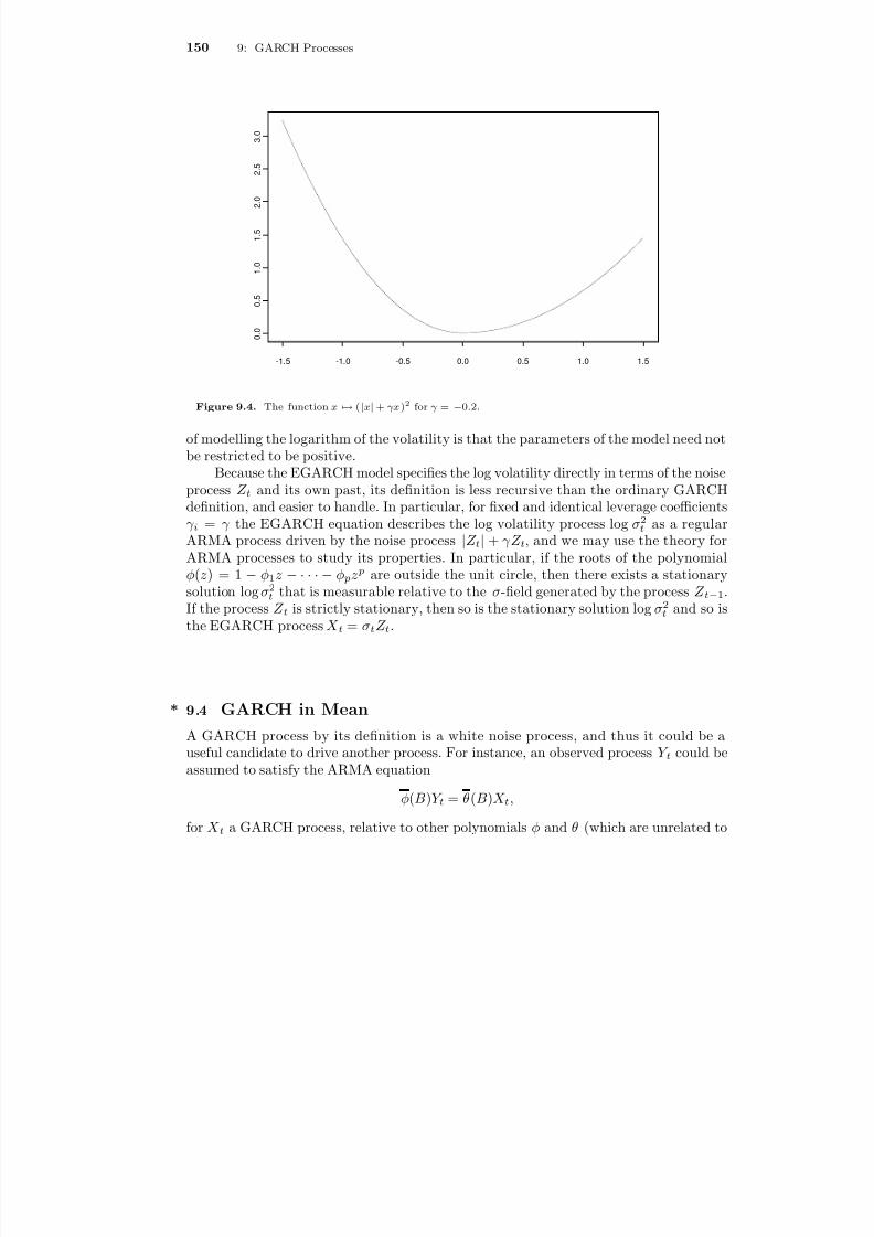
8/13/2019 van der Vaart: Time Series
http://slidepdf.com/reader/full/van-der-vaart-time-series 156/235
150 9: GARCH Processes
-1.5 -1.0 -0.5 0.0 0.5 1.0 1.5
0 . 0
0 . 5
1 . 0
1 . 5
2 . 0
2 . 5
3 . 0
Figure 9.4. The function x → ( |x | + γx ) 2 for γ = −0.2.
of modelling the logarithm of the volatility is that the parameters of the model need notbe restricted to be positive.
Because the EGARCH model species the log volatility directly in terms of the noiseprocess Z t and its own past, its denition is less recursive than the ordinary GARCHdenition, and easier to handle. In particular, for xed and identical leverage coefficientsγ i = γ the EGARCH equation describes the log volatility process log σ2
t as a regularARMA process driven by the noise process |Z t | + γZ t , and we may use the theory forARMA processes to study its properties. In particular, if the roots of the polynomialφ(z) = 1 −φ1 z − · · ·−φ pz p are outside the unit circle, then there exists a stationarysolution log σ2
t that is measurable relative to the σ-eld generated by the process Z t−1 .If the process Z t is strictly stationary, then so is the stationary solution log σ2
t and so isthe EGARCH process X t = σt Z t .
* 9.4 GARCH in Mean
A GARCH process by its denition is a white noise process, and thus it could be auseful candidate to drive another process. For instance, an observed process Y t could beassumed to satisfy the ARMA equation
φ(B )Y t = θ(B )X t ,
for X t a GARCH process, relative to other polynomials φ and θ (which are unrelated to

8/13/2019 van der Vaart: Time Series
http://slidepdf.com/reader/full/van-der-vaart-time-series 157/235
9.4: GARCH in Mean 151
φ and θ). One then says that Y t is “ARMA in the mean” and “GARCH in the variance”,or that Y t is an ARMA-GARCH series. Results on ARMA processes that hold for anydriving white noise process will clearly also hold in the present case, where the whitenoise process is a GARCH process.
9.19 EXERCISE. Let X t be a stationary GARCH process relative to polynomials φ andθ and let the time series Y t be the unique stationary solution to the equation φ(B )Y t =θ(B )X t , for φ and θ polynomials that have all their roots outside the unit disc. Let
F t be
the ltration generated by Y t . Show that var( Y t |F t−1) = var( X t |X t−1 , X t−2, . . .) almostsurely.
It has been found useful to go a step further and let also the conditional variance of the driving GARCH process appear in the mean model for the process Y t . Thus given aGARCH process X t with conditional variance process σ2
t = var( X t |F t−1) it is assumedthat Y t = f (σt , X t ) for a xed function f . The function f is assumed known up to anumber of parameters. For instance,
φ(B )Y t = ψσt + θ(B )X t ,
φ(B )Y t = ψσ2t + θ(B )X t ,
φ(B )Y t = ψ log σ2t + θ(B )X t .
These models are known as GARCH-in-mean , or GARCH-M models.

8/13/2019 van der Vaart: Time Series
http://slidepdf.com/reader/full/van-der-vaart-time-series 158/235
10State Space Models
A stochastic process X t is Markov if the conditional distribution of X t +1 given the “past”values X t , X t−1 , . . . depends on the “present” value X t only, for every t. The evolutionof a Markov process can be pictured as a sequence of moves in a “state space”, whereat each time t the process chooses a new state X t +1 based only on the current state X t ,and not on the past evolution. The current state thus contains all necessary informationfor the future.
The Markov structure obviously facilitates prediction, since only the current stateis needed to predict the future. It also permits a simple factorization of the likelihood.
Markov structure can be created in any time series by redening the states of theseries to incorporate enough past information. The “present state” should contain allinformation that is relevant for the next state. Specically, given an arbitrary time seriesX t , the process X t = ( X t , X t−1 , . . .) is Markov. However, the high complexity of thestate space of the process X t offsets the advantages of the Markov property.
General state space models take the idea of states that contain the relevant informa-tion as a basis, but go beyond Markov models. They typically consist of a specication of a Markov process together with an output process. Although they come from a differentbackground, hidden Markov models are almost identical structures.
The showpiece of state space modelling is the Kalman lter. This is an algorithm to
compute linear predictions for certain linear state space models, under the assumptionthat the parameters of the system are known. Because the formulas for the predictors,which are functions of the parameters and the outputs, can in turn be used to set upestimating equations for the parameters, the Kalman lter is also important for statisticalanalysis. We start discussing parameter estimation in Chapter 11.
10.1 Example (AR(1)) . A causal, stationary AR(1) process with i.i.d. innovations Z tis a Markov process: the “future value” X t +1 = φX t + Z t +1 given the “past values”X 1 , . . . , X t depends on the “present value” X t only. Specically, the conditional densityof X t +1 is given by
pX t +1 |X 1 ,...,X t (x) = pZ (x −φX t ).

8/13/2019 van der Vaart: Time Series
http://slidepdf.com/reader/full/van-der-vaart-time-series 159/235
10.1: Hidden Markov Models and State Spaces 153
The assumption of causality ensures that Z t +1 is independent of X 1 , . . . , X t . The Markovstructure allows to factorize the density of ( X 1 , . . . , X n ), as
pX 1 ,...,X n (X 1 , . . . , X n ) =n
t =2 pZ (X t −φX t−1) pX 1 (X 1).
This expression as a function of the unknown parameter φ is the likelihood for the model.
10.2 EXERCISE. How can a causal AR ( p) process be forced into Markov form? Give aprecise argument. Is “causal” needed?
10.1 Hidden Markov Models and State Spaces
A hidden Markov model consists of a Markov chain, but rather than the state at time t,we observe an “output” variable, which is generated by a mechanism which depends onthe state. This is illustrated in Figure 10.1, where the sequence . . . , X 1 , X 2 , . . . depictsa Markov chain, and . . . , Y 1 , Y 2 , . . . are the outputs at times 1 , 2, . . .. It is assumed thatgiven the state sequence . . . , X 1 , X 2 , . . ., the outputs . . . , Y 1 , Y 2 , . . . are independent, andthe conditional distribution of Y t given the states depends on X t only. Thus the arrowsin the picture indicate dependence relationships.
X 1 X 2 X 3. . .
X n −1 X n
Y 1 Y 2 Y 3. . .
Y n −1 Y n
Figure 10.1. Hidden Markov model.
The probabilistic properties of a hidden Markov process are simple. For instance,the joint sequence ( X t , Y t ) can be seen to be Markovian, and we can easily write downthe joint density of the variables ( X 1 , Y 1 , X 2 , Y 2 , . . . , X n , Y n ) as
p(x1) p(x2|x1) ×· · ·× p(xn |xn −1) p(y1 |x1) ×· · ·× p(yn |xn ).
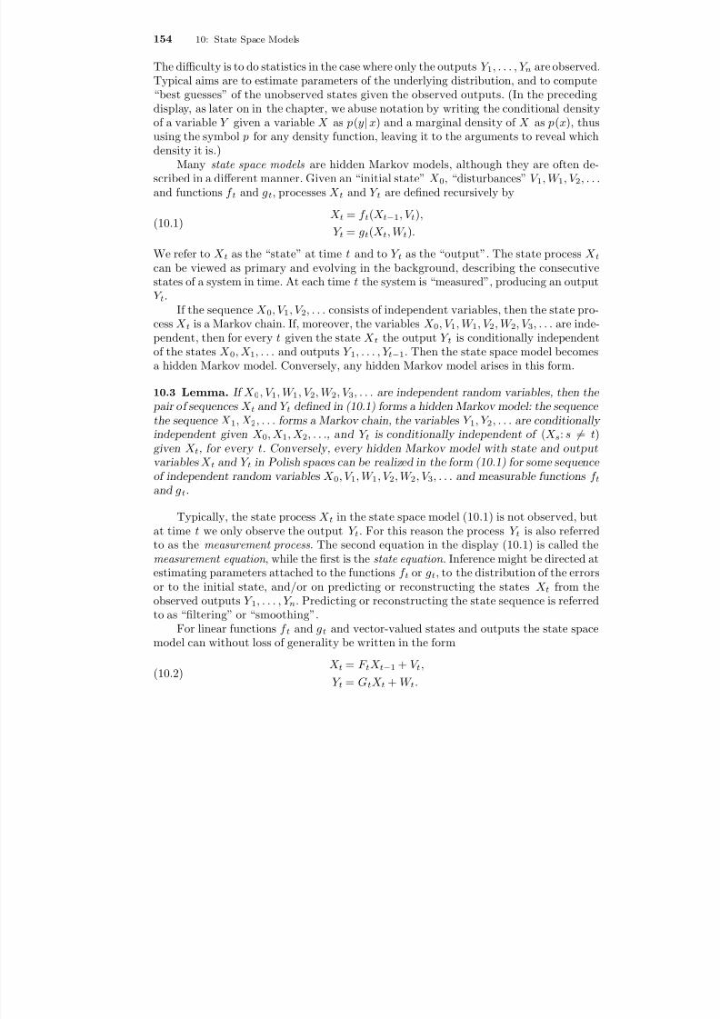
8/13/2019 van der Vaart: Time Series
http://slidepdf.com/reader/full/van-der-vaart-time-series 160/235
154 10: State Space Models
The difficulty is to do statistics in the case where only the outputs Y 1 , . . . , Y n are observed.Typical aims are to estimate parameters of the underlying distribution, and to compute“best guesses” of the unobserved states given the observed outputs. (In the precedingdisplay, as later on in the chapter, we abuse notation by writing the conditional densityof a variable Y given a variable X as p(y|x) and a marginal density of X as p(x), thususing the symbol p for any density function, leaving it to the arguments to reveal whichdensity it is.)
Many state space models are hidden Markov models, although they are often de-
scribed in a different manner. Given an “initial state” X 0 , “disturbances” V 1 , W 1 , V 2 , . . .and functions f t and gt , processes X t and Y t are dened recursively by
(10.1) X t = f t (X t−1 , V t ),
Y t = gt (X t , W t ).
We refer to X t as the “state” at time t and to Y t as the “output”. The state process X tcan be viewed as primary and evolving in the background, describing the consecutivestates of a system in time. At each time t the system is “measured”, producing an outputY t .
If the sequence X 0 , V 1 , V 2 , . . . consists of independent variables, then the state pro-cess X t is a Markov chain. If, moreover, the variables X 0 , V 1 , W 1 , V 2 , W 2 , V 3 , . . . are inde-pendent, then for every t given the state X t the output Y t is conditionally independent
of the states X 0 , X 1 , . . . and outputs Y 1 , . . . , Y t−1 . Then the state space model becomesa hidden Markov model. Conversely, any hidden Markov model arises in this form.
10.3 Lemma. If X 0 , V 1 , W 1 , V 2 , W 2 , V 3 , . . . are independent random variables, then the pair of sequences X t and Y t dened in (10.1) forms a hidden Markov model: the sequence the sequence X 1 , X 2 , . . . forms a Markov chain, the variables Y 1 , Y 2 , . . . are conditionally independent given X 0 , X 1 , X 2 , . . ., and Y t is conditionally independent of (X s : s = t)given X t , for every t. Conversely, every hidden Markov model with state and outputvariables X t and Y t in Polish spaces can be realized in the form (10.1) for some sequence of independent random variables X 0 , V 1 , W 1 , V 2 , W 2 , V 3 , . . . and measurable functions f tand gt .
Typically, the state process X t in the state space model (10.1) is not observed, but
at time t we only observe the output Y t . For this reason the process Y t is also referredto as the measurement process . The second equation in the display (10.1) is called themeasurement equation , while the rst is the state equation . Inference might be directed atestimating parameters attached to the functions f t or gt , to the distribution of the errorsor to the initial state, and/or on predicting or reconstructing the states X t from theobserved outputs Y 1 , . . . , Y n . Predicting or reconstructing the state sequence is referredto as “ltering” or “smoothing”.
For linear functions f t and gt and vector-valued states and outputs the state spacemodel can without loss of generality be written in the form
(10.2)X t = F t X t−1 + V t ,Y t = Gt X t + W t .
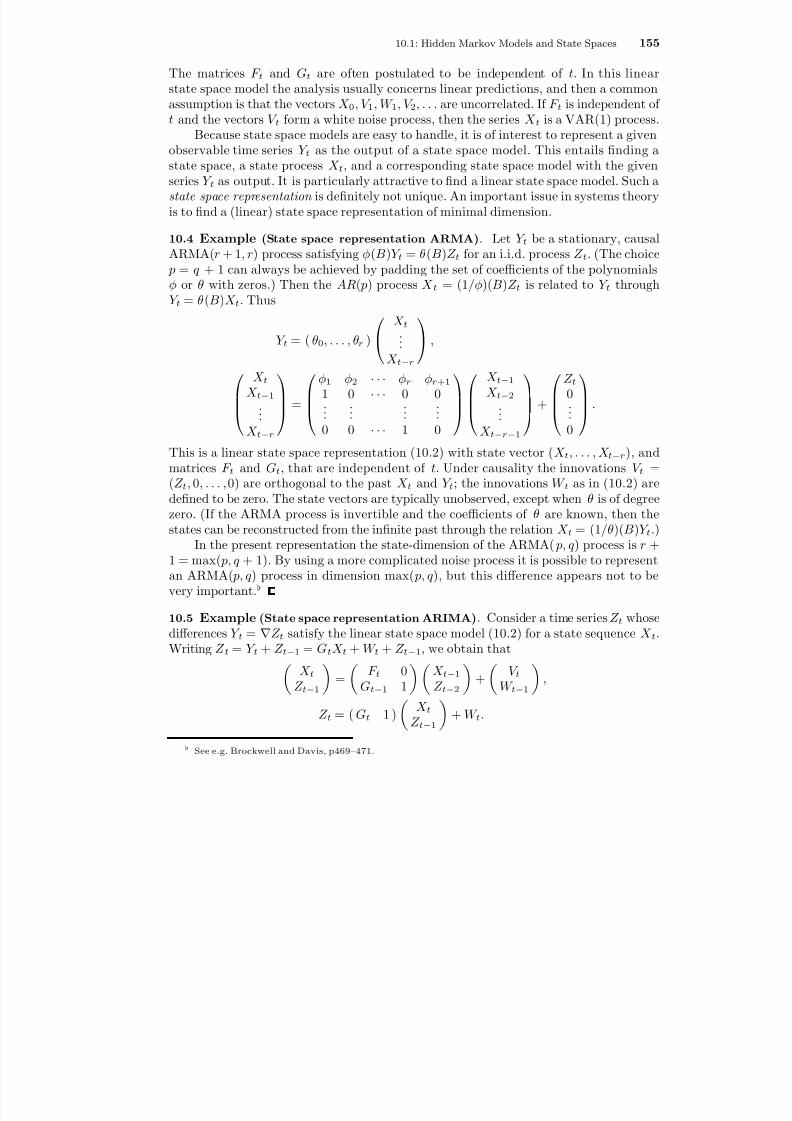
8/13/2019 van der Vaart: Time Series
http://slidepdf.com/reader/full/van-der-vaart-time-series 161/235
10.1: Hidden Markov Models and State Spaces 155
The matrices F t and Gt are often postulated to be independent of t. In this linearstate space model the analysis usually concerns linear predictions, and then a commonassumption is that the vectors X 0 , V 1 , W 1 , V 2 , . . . are uncorrelated. If F t is independent of t and the vectors V t form a white noise process, then the series X t is a VAR(1) process.
Because state space models are easy to handle, it is of interest to represent a givenobservable time series Y t as the output of a state space model. This entails nding astate space, a state process X t , and a corresponding state space model with the givenseries Y t as output. It is particularly attractive to nd a linear state space model. Such a
state space representation is denitely not unique. An important issue in systems theoryis to nd a (linear) state space representation of minimal dimension.
10.4 Example (State space representation ARMA) . Let Y t be a stationary, causalARMA( r + 1 , r ) process satisfying φ(B )Y t = θ(B )Z t for an i.i.d. process Z t . (The choice p = q + 1 can always be achieved by padding the set of coefficients of the polynomialsφ or θ with zeros.) Then the AR( p) process X t = (1 /φ )(B )Z t is related to Y t throughY t = θ(B )X t . Thus
Y t = ( θ0 , . . . , θr )X t...
X t−r
,
X tX t−1
...X t−r
=
φ1 φ2
· · · φr φr +1
1 0 · · · 0 0......
......
0 0 · · · 1 0
X t−1
X t−2...
X t−r −1
+
Z t0...0
.
This is a linear state space representation (10.2) with state vector ( X t , . . . , X t−r ), andmatrices F t and Gt , that are independent of t. Under causality the innovations V t =(Z t , 0, . . . , 0) are orthogonal to the past X t and Y t ; the innovations W t as in (10.2) aredened to be zero. The state vectors are typically unobserved, except when θ is of degreezero. (If the ARMA process is invertible and the coefficients of θ are known, then thestates can be reconstructed from the innite past through the relation X t = (1 /θ )(B )Y t .)
In the present representation the state-dimension of the ARMA( p, q ) process is r +1 = max( p, q + 1). By using a more complicated noise process it is possible to representan ARMA( p, q ) process in dimension max( p, q ), but this difference appears not to bevery important.
10.5 Example (State space representation ARIMA) . Consider a time series Z t whosedifferences Y t = Z t satisfy the linear state space model (10.2) for a state sequence X t .Writing Z t = Y t + Z t−1 = Gt X t + W t + Z t−1 , we obtain that
X tZ t−1
= F t 0G t−1 1
X t−1Z t−2
+ V tW t−1
,
Z t = ( G t 1 ) X tZ t−1
+ W t .
See e.g. Brockwell and Davis, p469–471.
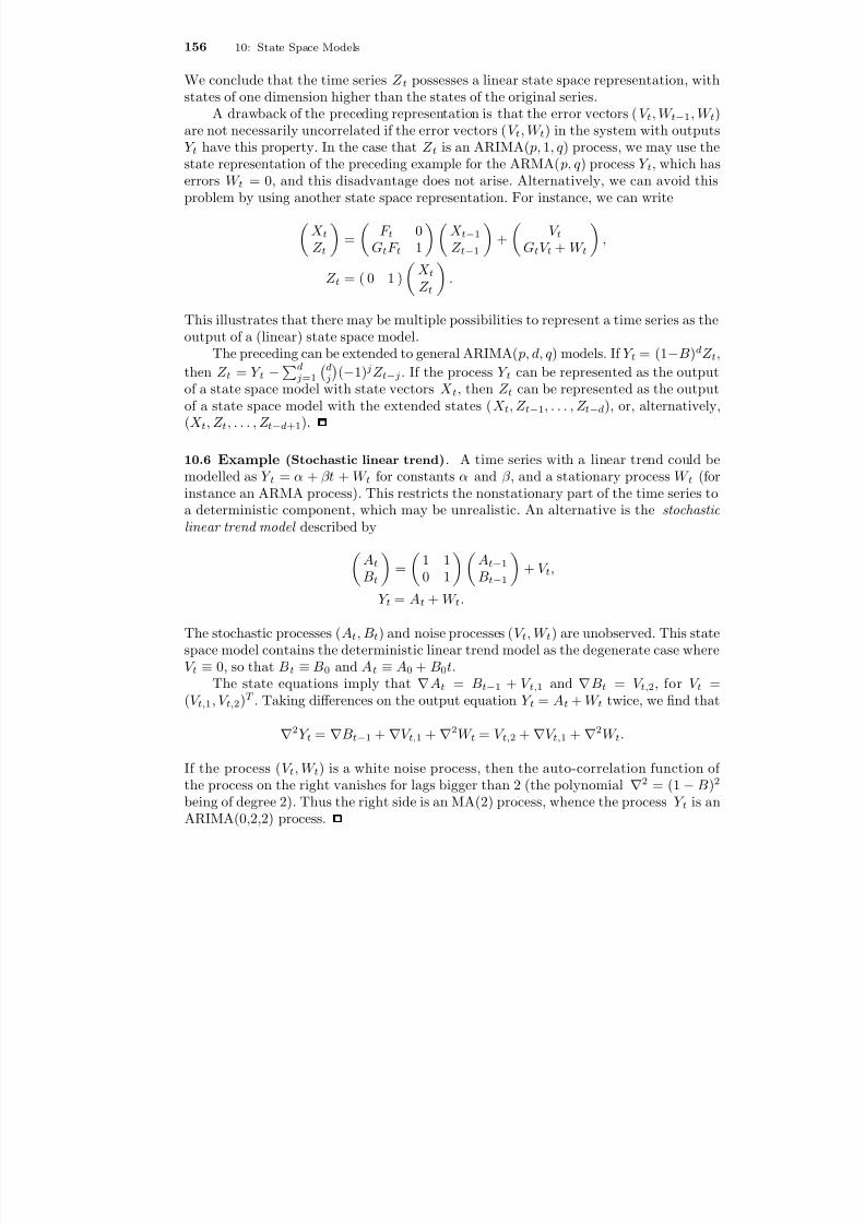
8/13/2019 van der Vaart: Time Series
http://slidepdf.com/reader/full/van-der-vaart-time-series 162/235
156 10: State Space Models
We conclude that the time series Z t possesses a linear state space representation, withstates of one dimension higher than the states of the original series.
A drawback of the preceding representation is that the error vectors ( V t , W t−1 , W t )are not necessarily uncorrelated if the error vectors ( V t , W t ) in the system with outputsY t have this property. In the case that Z t is an ARIMA( p, 1, q ) process, we may use thestate representation of the preceding example for the ARMA( p, q ) process Y t , which haserrors W t = 0, and this disadvantage does not arise. Alternatively, we can avoid thisproblem by using another state space representation. For instance, we can write
X tZ t
= F t 0Gt F t 1
X t−1Z t−1
+ V tGt V t + W t
,
Z t = ( 0 1 ) X tZ t
.
This illustrates that there may be multiple possibilities to represent a time series as theoutput of a (linear) state space model.
The preceding can be extended to general ARIMA( p, d, q ) models. If Y t = (1−B )dZ t ,then Z t = Y t − d
j =1dj (−1)j Z t−j . If the process Y t can be represented as the output
of a state space model with state vectors X t , then Z t can be represented as the outputof a state space model with the extended states ( X t , Z t−1 , . . . , Z t−d ), or, alternatively,
(X t , Z t , . . . , Z t−d+1 ).
10.6 Example (Stochastic linear trend) . A time series with a linear trend could bemodelled as Y t = α + βt + W t for constants α and β , and a stationary process W t (forinstance an ARMA process). This restricts the nonstationary part of the time series toa deterministic component, which may be unrealistic. An alternative is the stochastic linear trend model described by
AtB t
= 1 10 1
At−1B t−1
+ V t ,
Y t = At + W t .
The stochastic processes ( At , B t ) and noise processes ( V t , W t ) are unobserved. This statespace model contains the deterministic linear trend model as the degenerate case whereV t ≡ 0, so that B t ≡ B0 and A t ≡A0 + B0t .
The state equations imply that At = Bt−1 + V t, 1 and B t = V t, 2 , for V t =(V t, 1 , V t, 2)T . Taking differences on the output equation Y t = At + W t twice, we nd that
2 Y t = B t−1 + V t, 1 + 2W t = V t, 2 + V t, 1 + 2W t .
If the process ( V t , W t ) is a white noise process, then the auto-correlation function of the process on the right vanishes for lags bigger than 2 (the polynomial 2 = (1 −B )2
being of degree 2). Thus the right side is an MA(2) process, whence the process Y t is anARIMA(0,2,2) process.
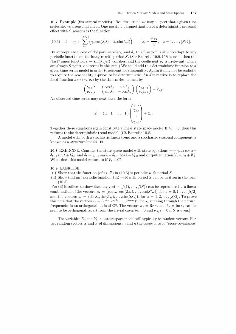
8/13/2019 van der Vaart: Time Series
http://slidepdf.com/reader/full/van-der-vaart-time-series 163/235
10.1: Hidden Markov Models and State Spaces 157
10.7 Example (Structural models) . Besides a trend we may suspect that a given timeseries shows a seasonal effect. One possible parametrization of a deterministic seasonaleffect with S seasons is the function
(10.3) t → γ 0 +S/ 2
s =1γ s cos(λ s t) + δ s sin(λ s t) , λs =
2πsS
, s = 1, . . . , S/ 2 .
By appropriate choice of the parameters γ s and δ s this function is able to adapt to any
periodic function on the integers with period S . (See Exercise 10.9. If S is even, then the“last” sinus function t → sin(λS/ 2 t) vanishes, and the coefficient δ s is irrelevant. Thereare always S nontrivial terms in the sum.) We could add this deterministic function to agiven time series model in order to account for seasonality. Again it may not be realisticto require the seasonality a-priori to be deterministic. An alternative is to replace thexed function s → (γ s , δ s ) by the time series dened by
γ s,tδ s,t
= cos λ s sin λ ssin λ s −cos λ s
γ s,t −1δ s,t −1
+ V s,t .
An observed time series may next have the form
Y t = ( 1 1 . . . 1 )
γ 1,tγ 2,t
.
..γ s,t
+ Z t .
Together these equations again constitute a linear state space model. If V t = 0, then thisreduces to the deterministic trend model. (Cf. Exercise 10.8.)
A model with both a stochastic linear trend and a stochastic seasonal component isknown as a structural model .
10.8 EXERCISE. Consider the state space model with state equations γ t = γ t−1 cosλ +δ t−1 sin λ + V t, 1 and δ t = γ t−1 sin λ −δ t−1 cosλ + V t, 2 and output equation Y t = γ t + W t .What does this model reduce to if V t ≡0?
10.9 EXERCISE.(i) Show that the function (of t
Z ) in (10.3) is periodic with period S .
(ii) Show that any periodic function f : Z →R with period S can be written in the form(10.3).
[For (ii) it suffices to show that any vector f (1), . . . , f (S ) can be represented as a linearcombination of the vectors as = cos λ s , cos(2λ s ), . . . , cos(Sλ s ) for s = 0, 1, . . . , S/ 2and the vectors bs = sin λ s , sin(2λ s ), . . . , sin(Sλ s ) , for s = 1 , 2, . . . , S/ 2 . To provethis note that the vectors es = ( eiλ s , e2iλ s . . . , einλ s )T for λs running through the naturalfrequencies is an orthogonal basis of C n . The vectors a s = Re es and bs = Im es can beseen to be orthogonal, apart from the trivial cases b0 = 0 and bS/ 2 = 0 if S is even.]
The variables X t and Y t in a state space model will typically be random vectors. Fortwo random vectors X and Y of dimensions m and n the covariance or “cross-covariance”

8/13/2019 van der Vaart: Time Series
http://slidepdf.com/reader/full/van-der-vaart-time-series 164/235
158 10: State Space Models
is the (m ×n) matrix Cov( X, Y ) = E( X −EX )(Y −EY )T . The random vectors X and Y are called “uncorrelated” if Cov( X, Y ) = 0, or equivalently if cov( X i , Y j ) = 0 for everypair ( i, j ). The linear span of a set of vectors is dened as the linear span of all theircoordinates. Thus this is a space of (univariate) random variables, rather than randomvectors! We shall also understand a projection operator Π, which is a map on the spaceof random variables, to act coordinatewise on vectors: if X is a vector, then Π X is thevector consisting of the projections of the coordinates of X . As a vector-valued operatora projection Π is still linear, in that Π( FX + Y ) = F ΠX + ΠY , for any matrix F and
random vectors X and Y .
10.2 Kalman FilteringThe Kalman lter is a recursive algorithm to compute best linear predictions of the statesX 1 , X 2 , . . . given observations Y 1 , Y 2 , . . . in the linear state space model (10.2). The corealgorithm allows to compute predictions Π t X t of the states X t given observed outputsY 1 , . . . , Y t . Here by “predictions” we mean Hilbert space projections. Given the timevalues involved, “reconstructions” would perhaps be more appropriate. “Filtering” is thepreferred term in systems theory. Given the reconstructions Π t X t , it is easy to compute
predictions of future states and future outputs. A next step is “Kalman smoothing”,which is the name for the reconstruction (again through projections) of the full statesequence X 1 , . . . , X n given the outputs Y 1 , . . . , Y n .
In the simplest situation the vectors X 0 , V 1 , W 1 , V 2 , W 2 , . . . are assumed uncorre-lated. We shall rst derive the lter under the more general assumption that the vectorsX 0 , (V 1 , W 1 ), (V 2 , W 2), . . . are uncorrelated, and in Section 10.2.4 we further relax thiscondition. The matrices F t and G t as well as the covariance matrices of the noise variables(V t , W t ) are assumed known.
By applying (10.2) recursively, we see that the vector X t is contained in the linearspan of the variables X 0 , V 1 , . . . , V t . It is immediate from (10.2) that the vector Y t iscontained in the linear span of X t and W t . These facts are true for every t N . It followsthat under our conditions the noise variables V t and W t are uncorrelated with all vectorsX s and Y s with s < t .
Let H 0 be a given closed linear subspace of L2(Ω, U , P) that contains the constants,and for t ≥ 0 let Πt be the orthogonal projection onto the space H t = H 0 +lin( Y 1 , . . . , Y t ).The space H 0 may be viewed as our “knowledge” at time 0; it may be H 0 = lin 1. Weassume that the noise vectors V 1 , W 1 , V 2 , . . . are orthogonal to H 0 . Combined with thepreceding this shows that the vector ( V t , W t ) is orthogonal to the space H t−1 , for everyt ≥ 1.
The Kalman lter consists of the recursions
· · ·→Πt−1 X t−1
Cov(Π t−1X t−1)Cov( X t−1)
(1)
→Πt−1 X t
Cov(Π t−1 X t )Cov(X t )
(2)
→Πt X t
Cov(Π t X t )Cov(X t )
→ ·· ·Thus the Kalman lter alternates between “updating the current state”, step (1), and

8/13/2019 van der Vaart: Time Series
http://slidepdf.com/reader/full/van-der-vaart-time-series 165/235
10.2: Kalman Filtering 159
“updating the prediction space”, step (2).Step (1) is simple. Because V t H 0 , Y 1 , . . . , Y t−1 by assumption, we have Π t−1V t =
0. Applying Π t to the state equation X t = F t X t−1 + V t we nd that, by the linearity of a projection,
Πt−1 X t = F t (Π t−1X t−1),
Cov(Π t−1 X t ) = F t Cov(Π t−1 X t−1)F T t ,
Cov(X t ) = F t Cov(X t−1)F T t + Cov( V t ).
This gives a complete description of step (1) of the algorithm.Step (2) is more involved, but also comes down to simple matrix computations. Thevector W t = Y t −Πt−1 Y t is known as the innovation at time t, because it is the part of Y tthat is not explainable at time t−1. It is orthogonal to H t−1 , and together with this spacespans H t . It follows that H t can be orthogonally decomposed as H t = H t−1 + lin W tand hence the projection onto H t is the sum of the projections onto the spaces H t−1 andlin W t . At the beginning of step (2) the vector W t is known, because we can write, usingthe measurement equation and the fact that Π t−1 W t = 0,
(10.4) W t = Y t −Πt−1Y t = Y t −Gt Πt−1X t = Gt (X t −Πt−1X t ) + W t .
The middle expression is easy to compute from the current values at the beginning of step (2). Applying this to projecting the variable X t , we nd
(10.5) Πt X t = Π t−1 X t + Λ t ˜W t , Λt = Cov( X t ,
˜W t ) Cov(
˜W t )−
1
.The matrix Λ t is chosen such that Λ t W t is the projection of X t onto lin W t . BecauseW t X t−1 the state equation equation yields Cov( X t , W t ) = Cov( V t , W t ). By the or-thogonality property of projections Cov( X t , X t −Πt−1X t ) = Cov( X t −Πt−1X t ). Com-bining this and the identity W t = Gt (X t −Πt−1X t ) + W t from (10.4), we compute
(10.6)
Cov( X t , W t ) = Cov( X t −Πt−1X t )GT t + Cov( V t , W t ),
Cov( W t ) = Gt Cov(X t −Πt−1 X t )GT t + G t Cov(V t , W t )
+ Cov( W t , V t )GT t + Cov( W t ),
Cov( X t −Πt−1X t ) = Cov( X t ) −Cov(Π t−1 X t ).
The matrix Cov( X t −Πt−1X t ) is the prediction error matrix at time t −1 and the lastequation follows by Pythagoras’ rule. To complete the recursion of step (2) we computefrom (10.5)
(10.7) Cov(Π t X t ) = Cov(Π t−1X t ) + Λ t Cov( W t )ΛT t .
Equations (10.5)–(10.7) give a complete description of step (2) of the Kalman recursion.The Kalman algorithm must be initialized in one of its two steps, for instance by
providing Π 0 X 1 and its covariance matrix, so that the recursion can start with a stepof type (2). It is here where the choice of H 0 plays a role. Choosing H 0 = lin (1) givespredictions using Y 1 , . . . , Y t as well as an intercept and requires that we know Π 0X 1 =EX 1 . It may also be desired that Π t−1X t is the projection onto lin (1 , Y t−1 , Y t−2 , . . .) fora stationary extension of Y t into the past. Then we set Π 0X 1 equal to the projection of X 1 onto H 0 = lin(1 , Y 0 , Y −1 , . . .).

8/13/2019 van der Vaart: Time Series
http://slidepdf.com/reader/full/van-der-vaart-time-series 166/235
160 10: State Space Models
10.2.1 Future States and Outputs
Predictions of future values of the state variable follow easily from Π t X t , becauseΠt X t + h = F t + h Πt X t + h −1 for any h ≥ 1. Given the predicted states, future outputscan be predicted from the measurement equation by Π t Y t + h = Gt + h Πt X t + h .
* 10.2.2 Missing Observations
A considerable attraction of the Kalman lter algorithm is the ease by which missingobservations can be accomodated. This can be achieved by simply lling in the missingdata points by “external” variables that are independent of the system. Suppose that(X t , Y t ) follows the linear state space model (10.2) and that we observe a subset ( Y t ) t T of the variables Y 1 , . . . , Y n . We dene a new set of matrices G t and noise variables W tby
Gt = Gt , W t = W t , t T ,
Gt = 0 , W t = W t , t / T,
for random vectors W t that are independent of the vectors that are already in the system.The choice W t = 0 is permitted. Next we set
X t = F t X t−1 + V t ,Y t = Gt X t + W t .
The variables ( X t , Y t ) follow a state space model with the same state vectors X t . Fort T the outputs Y t = Y t are identical to the outputs in the original system, whilefor t / T the output is Y t = W t , which is pure noise by assumption. Because the noisevariables W t cannot contribute to the prediction of the hidden states X t , best predictionsof states based on the observed outputs ( Y t )t T or based on Y 1 , . . . , Y n are identical.We can compute the best predictions based on Y 1 , . . . , Y n by the Kalman recursions,but with the matrices Gt and Cov( W t ) substituted for Gt and Cov( W t ). Because theY t with t / T will not appear in the projection formula, we can just as well set their“observed values” equal to zero in the computations.
* 10.2.3 Kalman Smoothing
Besides in predicting future states or outputs we may be interested in reconstructing thecomplete state sequence X 0 , X 1, . . . , X n from the outputs Y 1 , . . . , Y n . The computation of Πn X n is known as the ltering problem , and is step (2) of our description of the Kalmanlter. The computation of P n X t for t = 0 , 1, . . . , n −1 is known as the smoothing problem .For a given t it can be achieved through the recursions, with W n as given in (10.4),
Πn X tCov(X t , W n )
Cov(X t , X n −Πn −1X n ) →Πn +1 X t
Cov(X t , W n +1 )Cov(X t , X n +1 −Πn X n +1 )
, n = t, t + 1 , . . . .
The initial value at n = t of the recursions and the covariance matrices Cov( W n ) of theinnovations W n are given by (10.6)–(10.7), and hence can be assumed known.
8/13/2019 van der Vaart: Time Series
http://slidepdf.com/reader/full/van-der-vaart-time-series 167/235
10.2: Kalman Filtering 161
Because H n +1 is the sum of the orthogonal spaces H n and lin W n +1 , we have, as in(10.5),
Πn +1 X t = Π n X t + Λ t,n +1 W n +1 , Λt,n +1 = Cov( X t , W n +1 )Cov( W n +1 )−1 .
The recursion for the rst coordinate Π n X t follows from this and the recursionsfor the second and third coordinates, the covariance matrices Cov( X t , W n +1 ) andCov( X t , X n +1 −Πn X n +1 ).
Using in turn the state equation and equation (10.5), we nd
Cov( X t , X n +1 −Πn X n +1 ) = Cov X t , F n +1 (X n −Πn X n ) + V n +1
= Cov X t , F n +1 (X n −Πn −1X n + Λ n W n ) .
This readily gives the recursion for the third component, the matrix Λ n being knownfrom (10.5)–(10.6). Next using equation (10.4), we nd
Cov(X t , W n +1 ) = Cov( X t , X n +1 −Πn X n +1 )GT n +1 .
* 10.2.4 Lagged Correlations
In the preceding we have assumed that the vectors X 0 , (V 1 , W 1), (V 2 , W 2 ), . . . are uncor-related. An alternative assumption is that the vectors X 0 , V 1 , (W 1 , V 2), (W 2 , V 3), . . . areuncorrelated. (The awkward pairing of W t and V t +1 can be avoided by writing the stateequation as X t = F t X t−1 + V t−1 and next making the assumption as before.) Underthis condition the Kalman lter takes a slightly different form, where for economy of computation it can be useful to combine the steps (1) and (2).
Both possibilities are covered by the assumptions that- the vectors X 0 , V 1 , V 2 , . . . are orthogonal.- the vectors W 1 , W 2 , . . . are orthogonal.- the vectors V s and W t are orthogonal for all ( s, t ) except possibly s = t or s = t + 1.- all vectors are orthogonal to H 0 .
Under these assumptions step (2) of the Kalman lter remains valid as described. Step(1) must be adapted, because it is no longer true that Π t−1V t = 0.
Because V t H t−2 , we can compute Π t−1V t from the innovation decompositionH t−1 = H t−2 + lin W t−1 , as Πt−1V t = K t−1 W t−1 for the matrix
K t−1 = Cov( V t , W t−1) Cov( W t−1 )−1 .
Note here that Cov( V t , W t−1 ) = Cov( V t , W t−1 ), in view of (10.4). We replace the calcu-lations for step (1) by
Πt−1 X t = F t (Π t−1 X t−1) + K t W t−1 ,
Cov(Π t−1X t ) = F t Cov(Π t−1 X t−1)F T t + K t Cov( W t−1 )K T
t ,
Cov( X t ) = F t Cov(X t−1)F T t + Cov( V t ).

8/13/2019 van der Vaart: Time Series
http://slidepdf.com/reader/full/van-der-vaart-time-series 168/235
162 10: State Space Models
This gives a complete description of step (1) of the algorithm, under the assumption thatthe vector W t−1 , and its covariance matrix are kept in memory after the preceding step(2).
The smoothing algorithm goes through as stated except for the recursion for thematrices Cov( X t , X n −Πn −1X n ). Because Π n V n +1 may be nonzero, this becomes
Cov( X t , X n +1 −Πn X n +1 ) = Cov X t , X n −Πn −1X n )F T n +1 + Cov( X t , W n )ΛT
n F T n +1
+ Cov( X t , W n )K T n .
* 10.3 Nonlinear Filtering
The simplicity of the Kalman lter results from the combined linearity of the state spacemodel and the predictions. These lead to update formulas expressed in the terms of matrix algebra. The principle of recursive predictions can be applied more generally tocompute nonlinear predictions in nonlinear state space models, provided the conditionaldensities of the variables in the system are available and certain integrals involving thesedensities can be evaluated, analytically, numerically, or by stochastic simulation.
Abusing notation we write a conditional density of a variable X given another vari-able Y as p(x|y), and a marginal density of X as p(x). Consider the nonlinear statespace model (10.1), where we assume that the vectors X 0 , V 1 , W 1 , V 2 , . . . are indepen-dent. Then the outputs Y 1 , . . . , Y n are conditionally independent given the state sequenceX 0 , X 1 , . . . , X n , and the conditional law of a single output Y t given the state sequencedepends on X t only. In principle the (conditional) densities p(x0), p(x1|x0), p(x2 |x1), . . .and the conditional densities p(yt |xt ) of the outputs are available from the form of thefunctions f t and gt and the distributions of the noise variables ( V t , W t ). The joint densityof states up till time n + 1 and outputs up till time n in this hidden Markov model canbe expressed in these densities as
(10.8) p(x0 ) p(x1 |x0 ) · · · p(xn +1 |xn ) p(y1|x1) p(y2|x2 ) · · · p(yn |xn ).
The marginal density of the outputs ( Y 1 , . . . , Y n ) is obtained by integrating this functionrelative to ( x0 , . . . , xn +1 ). The conditional density of the state sequence ( X 0 , . . . , X n +1 )given the outputs is proportional to the function in the display, the norming constantbeing the marginal density of the outputs. In principle, this allows the computationof all conditional expectations E( X t |Y 1 , . . . , Y n ), the (nonlinear) “predictions” of thestate. However, because this approach expresses these predictions as a quotient of n + 1-dimensional integrals, and n may be large, this is unattractive unless the integrals canbe evaluated easily.
An alternative for nding predictions is a recursive scheme for calculating conditionaldensities, of the form
·· · → p(xt−1|yt−1 , . . . , y1)(1)→ p(x t |yt−1 , . . . , y1)
(2)→ p(x t |yt , . . . , y1) → ·· ·.

8/13/2019 van der Vaart: Time Series
http://slidepdf.com/reader/full/van-der-vaart-time-series 169/235
10.3: Nonlinear Filtering 163
This is completely analogous to the updates of the linear Kalman lter: the recursionsalternate between “updating the state”, (1), and “updating the prediction space”, (2).
Step (1) can be summarized by the formula
p(xt |yt−1 , . . . , y1) = p(x t |xt−1 , yt−1 , . . . , y1) p(x t−1 |yt−1 , . . . , y1) dµt−1(x t−1)
= p(x t |xt−1) p(x t−1|yt−1 , . . . , y1) dµt−1(xt−1 ).
The second equality follows from the conditional independence of the vectors X t andY t−1 , . . . , Y 1 given X t−1 . This is a consequence of the form of X t = f t (X t−1 , V t )and the independence of V t and the vectors X t−1 , Y t−1 , . . . , Y 1 (which are functions of X 0 , V 1 , . . . , V t−1 , W 1 , . . . , W t−1 ).
To obtain a recursion for step (2) we apply Bayes formula to the conditional densityof the pair ( X t , Y t ) given Y t−1 , . . . , Y 1 to obtain
p(x t |yt , . . . , y1) = p(yt |x t , yt−1 , . . . , y1) p(x t |yt−1 , . . . , y1)
p(yt |x t , yt−1 , . . . , y1) p(x t |yt−1 , . . . , y1) dµt (xt )
= p(yt |x t ) p(x t |yt−1 , . . . , y1)
p(yt |yt−1 , . . . , y1) .
The second equation is a consequence of the fact that Y t = gt (X t , W t ) is conditionally
independent of Y t−1 , . . . , Y 1 given X t . The conditional density p(yt |yt−1 , . . . , y1) in thedenominator is a nuisance, because it will rarely be available explicitly, but acts only asa norming constant.
The preceding formulas are useful only if the integrals can be evaluated. If analyticalevaluation is impossible, then perhaps numerical methods or stochastic simulation couldbe of help.
If stochastic simulation is the method of choice, then it may be attractive to ap-ply Markov Chain Monte Carlo for direct evaluation of the joint law, without recur-sions. The idea is to simulate a sample from the conditional density ( x0 , . . . , x n +1 ) → p(x0 , . . . , x n +1 |y1 , . . . , yn ) of the states given the outputs. The biggest challenge isthe dimensionality of this conditional density. The Gibbs sampler overcomes this bysimulating recursively from the marginal conditional densities p(xt |x−t , y1 , . . . , yn )of the single variables X t given the outputs Y 1 , . . . , Y n and the vectors X −t =
(X 0 , . . . , X t−1 , X t +1 , . . . , X n +1 ) of remaining states. These iterations yield a Markovchain, with the target density ( x0 , . . . , x n +1 ) → p(x0 , . . . , x n +1 |y1 , . . . , yn ) as a station-ary density, and under some conditions the iterates of the chain can eventually be thoughtof as a (dependent) sample from (approximately) this target density. We refer to the lit-erature for general discussion of the Gibbs sampler, but shall show that these marginaldistributions are relatively easy to obtain for the general state space model (10.1).
Under independence of the vectors X 0 , V 1 , W 1 , V 2 , . . . the joint density of states andoutputs takes the hidden Markov form (10.8). The conditional density of X t given theother vectors is proportional to this expression viewed as function of xt only. Only threeterms of the product depend on x t and hence we nd
p(xt |x−t , y1 , . . . , yn ) p(x t |x t−1) p(x t +1 |x t ) p(yt |xt ).
8/13/2019 van der Vaart: Time Series
http://slidepdf.com/reader/full/van-der-vaart-time-series 170/235
164 10: State Space Models
The norming constant is a function of the conditioning variables x−t , y1 , . . . , yn only andcan be recovered from the fact that the left side is a probability density as a functionof xt . A closer look will reveal that it is equal to p(yt |x t−1 , x t +1 ) p(xt +1 |xt−1). However,many simulation methods, in particular the popular Metropolis-Hastings algorithm, canbe implemented without an explicit expression for the proportionality constant. Theforms of the three densities on the right side should follow from the specication of thesystem.
The assumption that the variables X 0 , V 1 , W 2 , V 2 , . . . are independent may be too
restrictive, although it is natural to try and construct the state variables so that it issatised. Somewhat more complicated formulas can be obtained under more generalassumptions. Assumptions that are in the spirit of the preceding derivations in thischapter are:(i) the vectors X 0 , X 1 , X 2 , . . . form a Markov chain.
(ii) the vectors Y 1 , . . . , Y n are conditionally independent given X 0 , X 1 , . . . , X n +1 .(iii) for each t 1, . . . , n the vector Y t is conditionally independent of the vector
(X 0 , . . . , X t−2 , X t +2 , . . . , X n +1 ) given (X t−1 , X t , X t +1 ).The rst assumption is true if the vectors X 0 , V 1 , V 2 , . . . are independent. The secondand third assumptions are certainly satised if all noise vectors X 0 , V 1 , W 1 , V 2 , W 2 , V 3 , . . .are independent. The exercises below give more general sufficient conditions for (i)–(iii)in terms of the noise variables.
In comparison to the hidden Markov situation considered previously not muchchanges. The joint density of states and outputs can be written in a product form similarto (10.8), the difference being that each conditional density p(yt |x t ) must be replaced by p(yt |xt−1 , x t , x t +1 ). The variable x t then occurs in ve terms of the product and hencewe obtain
p(xt |x−t , y1 , . . . , yn ) p(xt +1 |xt ) p(xt |x t−1)×× p(yt−1|x t−2 , x t−1 , x t ) p(yt |xt−1 , x t , x t +1 ) p(yt +1 |xt , x t +1 , x t +2 ).
This formula is general enough to cover the case of the ARV model discussed in the nextsection.
10.10 EXERCISE. Suppose that X 0 , V 1 , W 1 , V 2 , W 2 , V 3 , . . . are independent, and denestates X t and outputs Y t by (10.1). Show that (i)–(iii) hold, where in (iii) the vector Y t
is even conditionally independent of ( X s : s = t) given X t .10.11 EXERCISE. Suppose that X 0 , V 1 , V 2 , . . . , Z 1 , Z 2, . . . are independent, and denestates X t and outputs Y t through (10.2) with W t = ht (V t , V t +1 , Z t ) for measurablefunctions ht . Show that (i)–(iii) hold. [Under (10.2) there exists a measurable bijectionbetween the vectors ( X 0 , V 1 , . . . , V t ) and ( X 0 , X 1 , . . . , X n ), and also between the vectors(X t , X t−1 , X t +1 ) and ( X t , V t , V t +1 ). Thus conditioning on ( X 0 , X 1 , . . . , X n +1 ) is the sameas conditioning on ( X 0 , V 1 , . . . , V n +1 ) or on (X 0 , V 1 , . . . , V n , X t−1 , X t , X t +1 ).]
* 10.12 EXERCISE. Show that the condition in the preceding exercise that W t =h t (V t , V t +1 , Z t ) for Z t independent of the other variables is equivalent to the conditionalindependence of W t and X 0 , V 1 , . . . , V n , W s : s = t given V t , V t +1 .
8/13/2019 van der Vaart: Time Series
http://slidepdf.com/reader/full/van-der-vaart-time-series 171/235
10.4: Stochastic Volatility Models 165
10.4 Stochastic Volatility Models
The term “volatility”, which we have used at multiple occasions to describe the “mov-ability” of a time series, appears to have its origins in the theory of option pricing. TheBlack-Scholes model for pricing an option on a given asset with price S t is based on adiffusion equation of the type
dS t = µt S t dt + σt S t dB t .
Here Bt is a Brownian motion process and µt and σt are stochastic processes, whichare usually assumed to be adapted to the ltration generated by the process S t . In theoriginal Black-Scholes model the process σt is assumed constant, and the constant isknown as the “volatility” of the process S t .
The Black-Scholes diffusion equation can also be written in the form
log S tS 0
= t
0(µs − 1
2 σ2s ) ds +
t
0σs dB s .
If µ and σ are deterministic processes this shows that the log returns log S t /S t−1 overthe intervals ( t −1, t ] are independent, normally distributed variables ( t = 1, 2, . . .) withmeans
tt−1(µs − 1
2 σ2s ) ds and variances
tt−1 σ2
s ds. In other words, if these means andvariances are denoted by µt and σ2
t , then the variables
Z t = logS t /S t−1 −µt
σt
are an i.i.d. sample from the standard normal distribution. The standard deviation σtcan be viewed as an “average volatility” over the interval ( t −1, t ]. If the processes µtand σt are not deterministic, then the process Z t is not necessarily Gaussian. However,if the unit of time is small, so that the intervals ( t − 1, t ] correspond to short timeintervals in real time, then it is still believable that the variables Z t are approximatelynormally distributed. In that case it is also believable that the processes µt and σt areapproximately constant and hence these processes can replace the averages µt and σt .Usually, one even assumes that the process µt is constant in time. For simplicity of notation we shall take µt to be zero in the following, leading to a model of the form
log S t /S t−1 = σt Z t ,for standard normal variables Z t and a “volatility” process σt . The choice µt = µt −1
2 σ2t =
0 corresponds to modelling under the “risk-free” martingale measure, but is made hereonly for convenience.
There is ample empirical evidence that models with constant volatility do not tobserved nancial time series. In particular, this has been documented through a compar-ison of the option prices predicted by the Black-Scholes formula to the observed prices onthe option market. Because the Black-Scholes price of an option on a given asset dependsonly on the volatility parameter of the asset price process, a single parameter volatilitymodel would allow to calculate this parameter from the observed price of an option onthis asset, by inversion of the Black-Scholes formula. Given a range of options written on
8/13/2019 van der Vaart: Time Series
http://slidepdf.com/reader/full/van-der-vaart-time-series 172/235
8/13/2019 van der Vaart: Time Series
http://slidepdf.com/reader/full/van-der-vaart-time-series 173/235
10.4: Stochastic Volatility Models 167
in other situations we would have written V t . It is meant to support the idea that σt isdetermined at time t −1.)
An ARV stochastic volatility process is a nonlinear state space model. It induces alinear state space model for the log volatilities and log absolute log returns of the form
log σt = ( α φ ) 1log σt−1
+ V t−1
log |X t | = log σt + log |Z t |.In order to take the logarithm of the observed series X t it was necessary to take theabsolute value |X t | rst. Usually this is not a serious loss of information, because thesign of X t is equal to the sign of Z t , and this is a Bernoulli 1
2 series if Z t is symmetricallydistributed.
The linear state space form allows the application of the Kalman lter to computebest linear projections of the unobserved log volatilities log σt based on the observed logabsolute log returns log |X t |. Although this approach is computationally attractive, adisadvantage is that the best predictions of the volatilities σt based on the log returnsX t may be much better than the exponentials of the best linear predictions of the logvolatilities log σt based on the log returns. Forcing the model in linear form is not entirelynatural here. However, the computation of best nonlinear predictions is involved. MarkovChain Monte Carlo methods are perhaps the most promising technique, but are highlycomputer-intensive.
An ARV process X t is a martingale difference series relative to its natural ltration
F t = σ(X t , X t−1 , . . .). To see this we rst note that by causality σt σ(V t−1 , V t−2 , . . .),whence F t is contained in the ltration Gt = σ(V s , Z s : s ≤ t). The process X t is actuallyalready a martingale difference relative to this bigger ltration, because by the assumedindependence of Z t from Gt−1
E( X t |Gt−1) = σt E( Z t |Gt−1 ) = 0 .
A fortiori the process X t is a martingale difference series relative to the ltration F t .There is no correspondingly simple expression for the conditional variance process
E( X 2t |F t−1) of an ARV series. By the same argument
E(X 2t |Gt−1) = σ2t EZ 2t .
If EZ 2t = 1 it follows that E( X
2t |F t−1) = E( σ
2t |F t−1), but this is intractable for furtherevaluation. In particular, the process σ2
t is not the conditional variance process, unlikein the situation of a GARCH process. Correspondingly, in the present context, in whichσt is considered the “volatility”, the volatility and conditional variance processes do notcoincide.
10.13 EXERCISE. One denition of a volatility process σt of a time series X t is aprocess σt such that X t /σ t is an i.i.d. standard normal series. Suppose that X t = σt Z tis a GARCH process with conditional variance process ˜ σ2
t and driven by an i.i.d. processZ t . If Z t is standard normal, show that ˜ σt qualies as a volatility process. [Trivial.] If Z tis a t p-process show that there exists a process S 2t with a chisquare distribution with pdegrees of freedom such that √ pσt /S t qualies as a volatility process.

8/13/2019 van der Vaart: Time Series
http://slidepdf.com/reader/full/van-der-vaart-time-series 174/235
168 10: State Space Models
10.14 EXERCISE. In the ARV model is σt measurable relative to the σ-eld generatedby X t−1 , X t−2 , . . .? Compare with GARCH models.
In view of the analogy with continuous time diffusion processes the assumption thatthe variables ( V t , Z t ) in (10.9)–(10.10) are normally distributed could be natural. Thisassumption certainly helps to compute moments of the series. The stationary solutionlog σt of the auto-regressive equation (10.9) is given by (for |φ| < 1)
log σt = ∞j =0
φj (V t−1−j + α) = ∞j =0
φj V t−1−j + α1 −φ
.
If the time series V t is i.i.d. Gaussian with mean zero and variance σ2 , then it follows thatthe variable log σt is normally distributed with mean α/ (1−φ) and variance σ2 / (1−φ2).The Laplace transform E exp( aZ ) of a standard normal variable Z is given by exp( 1
2 a2).Therefore, under the normality assumption on the process V t it is straightforward tocompute that, for p > 0,
E|X t | p = E e p log σ t E|Z t | p = exp 12
σ2 p2
1 −φ2 + αp1 −φ
E|Z t | p.
Consequently, the kurtosis of the variables X t can be computed to be
κ4(X ) = e4σ 2 / (1 −φ2 ) κ4(Z ).
If follows that the time series X t possesses a larger kurtosis than the series Z t . This istrue even for φ = 0, but the effect is more pronounced for values of φ that are closeto 1, which are commonly found in practice. Thus the ARV model is able to explainleptokurtic tails of an observed time series.
Under the assumption that the variables ( V t , Z t ) are i.i.d. and bivariate normallydistributed, it is also possible to compute the auto-correlation function of the squaredseries X 2t explicitly. If δ = ρ(V t , Z t ) is the correlation between the variables V t andZ t , then the vectors (log σt , log σt + h , Z t ) possess a three-dimensional normal distributionwith covariance matrix
β 2 β 2 φh 0β 2φh β 2 φh−1δσ
0 φh −1δσ 1, β 2 =
σ2
1 −φ2 .
Some calculations show that the auto-correlation function of the square process is givenby
ρX 2 (h) = (1 + 4δ 2σ2 φ2h −2)e4σ 2 φh / (1 −φ2 ) −1
3e4σ 2 / (1 −φ 2 ) −1 , h > 0.
The auto-correlation is positive at positive lags and decreases exponentially fast to zero,with a rate depending on the proximity of φ to 1. For values of φ close to 1, the decreaseis relatively slow.
8/13/2019 van der Vaart: Time Series
http://slidepdf.com/reader/full/van-der-vaart-time-series 175/235

8/13/2019 van der Vaart: Time Series
http://slidepdf.com/reader/full/van-der-vaart-time-series 176/235

8/13/2019 van der Vaart: Time Series
http://slidepdf.com/reader/full/van-der-vaart-time-series 177/235
11.1: Yule-Walker Estimators 171
the assumption that the series is causal. This is equivalent to requiring that all roots of the polynomial φ(z) = 1 −φ1 z −· · ·−φ pz p are outside the unit circle.
Under causality the best linear predictor of X p+1 based on 1, X p, . . . , X 1 is given byΠ pX p+1 = µ + φ1 (X p −µ) + · · ·+ φ p(X 1 −µ). (See Section 8.4.) Alternatively, the bestlinear predictor can be obtained by solving the general prediction equations (2.4). Thisshows that the parameters φ1 , . . . , φ p satisfy
γ X (0) γ X (1) · · · γ X ( p −1)
γ X (1) γ X (0) · · · γ X ( p −2)......
...γ X ( p−1) γ X ( p −2) · · · γ X (0)
φ1
φ2...φ p
=
γ X (1)
γ X (2)...γ X ( p)
.
We abbreviate this system of equations by Γ p φ p = γ p. These equations, known as theYule-Walker equations , express the parameters into second moments of the observations.The Yule-Walker estimators are dened by replacing the true auto-covariances γ X (h) bytheir sample versions ˆγ n (h) and next solving for φ1 , . . . , φ p. This leads to the estimators
φ p: =
φ1φ2...
φ p
=
γ n (0) γ n (1) · · · γ n ( p −1)γ n (1) γ n (0) · · · γ n ( p −2)
......
...
γ n ( p −1) γ n ( p−2) · · · γ n (0)
−1 γ n (1)γ n (2)
...
γ n ( p)
=: Γ−1 p γ p.
The parameter σ2 is by denition the variance of Z p+1 , which is the prediction errorX p+1 −Π pX p+1 when predicting X p+1 by the preceding observations, under the assump-tion that the time series is causal. By the orthogonality of the prediction error and thepredictor Π pX p+1 and Pythagoras’ rule,
(11.1) σ2 = E( X p+1 −µ)2 −E(Π pX p+1 −µ)2 = γ X (0) − φT p Γ p φ p.
We dene an estimator ˆ σ2 by replacing all unknowns by their moment estimators, i.e.
σ2 = γ n (0) − φT
p Γ p φ p.
11.1 EXERCISE. An alternative method to derive the Yule-Walker equations is to workout the equations cov φ(B )(X t − µ), X t−k − µ = cov Z t , j ≥0 ψj Z t−j −k for k =0, . . . , p. Check this. Do you need causality? What if the time series would not be causal?
11.2 EXERCISE. Show that the matrix Γ p is invertible for every p. [Suggestion: writeα T Γ pα in terms of the spectral density.]
Another reasonable method to nd estimators is to start from the fact that the truevalues of φ1 , . . . , φ p minimize the expectation
(β 1 , . . . , β p) → E X t −µ −β 1(X t−1 −µ) −· · ·−β p(X t− p −µ) 2 .

8/13/2019 van der Vaart: Time Series
http://slidepdf.com/reader/full/van-der-vaart-time-series 178/235
8/13/2019 van der Vaart: Time Series
http://slidepdf.com/reader/full/van-der-vaart-time-series 179/235
11.1: Yule-Walker Estimators 173
Proof. We can assume without loss of generality that µ = 0. The AR equationsφ(B )X t = Z t for t = n, n −1, . . . , p + 1 can be written in the matrix form
X nX n −1
...X p+1
=
X n −1 X n −2 · · · X n − pX n −2 X n −3 · · · X n − p−1
......
...X p X p−1 · · · X 1
φ1φ2...
φ p
+
Z nZ n −1
...Z p+1
= Dn φ p + Z n ,
for Z n the vector with coordinates Z t + X n φi , and Dn the “design matrix” as before.We can solve φ p from this as, writing X n for the vector on the left,
φ p = ( D T n D n )−1D T
n ( X n − Z n ).
Combining this with the analogous representation of the least squares estimators φj wend
√ n( φ p − φ p) =1n
D T n Dn
−1 1√ n D T
n Z n −X n (1 −
i
φi ) 1 .
Because X t is an auto-regressive process, it possesses a representation X t = j ψj Z t−jfor a sequence ψj with
j |ψj | < ∞. Therefore, the results of Chapter 8 apply and show
that n−1D T n Dn
P
→ Γ p. (In view of Problem 11.2 this also shows that the matrix D T
n Dn
is invertible, as was assumed implicitly in the preceding.)In view of Slutsky’s lemma it now suffices to show that
1√ n D T
n Z n N (0, σ2Γ p), 1
√ n D T n 1X n P
→ 0.
A typical coordinate of the last vector is (for h = 1 , . . . , p)
1√ n
n
t = p+1(X t−h −X n )X n =
1√ n
n
t = p+1X t−h X n −
n − p√ n X
2n .
In view of Theorem 4.5 and the assumption that µ = 0, the sequence √ nX n convergesin distribution. Hence both terms on the right side are of the order OP (1/ √ n).
A typical coordinate of the rst vector is (for h = 1 , . . . , p)
1√ n
n
t = p+1
(X t−h −X n )Z t = 1√ n
n − p
t =1Y t + OP
1√ n ,
for Y t = X p−h + t Z p+ t . By causality of the series X t we have Z p+ t X p−s + t for s > 0and hence E Y t = E X p−s + t EZ p+ t = 0 for every t. The same type of arguments as inChapter 5 will give us the asymptotic normality of the sequence √ nY n , with asymptoticvariance
∞
g= −∞γ Y (g) =
∞
g= −∞EX p−h + g Z p+ gX p−h Z p.

8/13/2019 van der Vaart: Time Series
http://slidepdf.com/reader/full/van-der-vaart-time-series 180/235
174 11: Moment and Least Squares Estimators
In this series all terms with g > 0 vanish because Z p+ g is independent of ( X p−h + g , X p−h , Z p),by the assumption of causality and the fact that Z t is an i.i.d. sequence. All terms withg < 0 vanish by symmetry. Thus the series is equal to γ Y (0) = E X 2 p−h Z 2 p = γ X (0)σ2 ,which is the diagonal element of σ2 Γ p. This concludes the proof of the convergence indistribution of all marginals of n−1/ 2D T
n Z n . The joint convergence is proved in similarly,
with the help of the Cramer-Wold device.This concludes the proof of the asymptotic normality of the least squares estima-
tors. The Yule-Walker estimators can be proved to be asymptotically equivalent to theleast squares estimators, in that the difference is of the order oP (1/ √ n). Next we applySlutsky’s lemma.
11.4 EXERCISE. Show that the time series Y t in the preceding proof is strictly station-ary.
* 11.5 EXERCISE. Give a complete proof of the asymptotic normality of √ nY n as denedin the preceding proof, along the lines sketched, or using the fact nY n is a martingale.
11.1.1 Order SelectionIn the preceding derivation of the least squares and Yule-Walker estimators the order pof the AR process is assumed known a-priori. Theorem 11.3 is false if X t
−µ were in
reality an AR ( p0) process of order p0 > p. In that case φ1 , . . . φ p are estimators of thecoefficients of the best linear predictor based on p observations, but need not convergeto the p0 coefficients φ1 , . . . , φ p0 . On the other hand, Theorem 11.3 remains valid if theseries X t is an auto-regressive process of “true” order p0 strictly smaller than the order p used to dene the estimators. This follows because for p0 ≤ p an AR( p0) processis also an AR( p) process, albeit that φ p0 +1 , . . . , φ p are zero. Theorem 11.3 shows that“overtting” (choosing too big an order) does not cause great harm: if φ( p)
1 , . . . , φ( p)j are
the Yule-Walker estimators when tting an AR( p) model and the observations are anAR( p0) process with p0 ≤ p, then
√ nφ( p)j
N 0, σ2(Γ−1 p )j,j , j = p0 + 1 , . . . , p .
It is recomforting that the estimators of the “unnecessary” coefficients φ p0 +1 , . . . , φ p
converge to zero at rate 1 / √ n. However, there is also a price to be paid by overtting.By Theorem 11.3, if tting an AR( p)-model, then the estimators of the rst p0 coefficientssatisfy
√ nφ( p)
1...
φ( p) p0
−φ1...
φ p0
N 0, σ2(Γ−1 p )s,t =1 ,...,p 0 .
The covariance matrix in the right side, the ( p0 × p0) upper principal submatrix of the( p× p) matrix Γ −1
p , is not equal to Γ−1 p0 , which would be the asymptotic covariance matrix
if we tted an AR model of the “correct” order p0 . In fact, it is bigger in that
(Γ−1 p )s,t =1 ,...,p 0 −Γ−1
p0 ≥0.

8/13/2019 van der Vaart: Time Series
http://slidepdf.com/reader/full/van-der-vaart-time-series 181/235
11.1: Yule-Walker Estimators 175
Here A ≥0 means that the matrix A is nonnegative denite. In particular, the diagonalelements of these matrices, which are the differences of the asymptotic variances of theestimators φ( p)
j and the estimators φ( p0 )j , are nonnegative. Thus overtting leads to more
uncertainty in the estimators of both φ1 , . . . , φ p0 and φ p0 +1 , . . . , φ p . Fitting an auto-regressive process of very high order p increases the chance of having the model t wellto the data, but generally will result in poor estimates of the coefficients, which renderthe nal outcome less useful.
* 11.6 EXERCISE. Prove the assertion that the given matrix is nonnegative denite.
In practice we do not know the correct order to use. A suitable order is oftendetermined by a preliminary data-analysis, such as an inspection of the plot of thesample partial auto-correlation function. More formal methods are discussed within thegeneral context of maximum likelihood estimation in Chapter 13.
11.7 Example. If we t an AR(1) process to observations of an AR(1) series, then theasymptotic covariance of √ n(φ1 − φ1 ) is equal to σ2 Γ−1
1 = σ2 /γ X (0). If to this sameprocess we t an AR(2) process, then we obtain estimators ( φ(2)
1 , φ(2)2 ) (not related to
the earlier φ1) such that √ n(φ(2)1 −φ1 , φ(2)
2 ) has asymptotic covariance matrix
σ2Γ−12 = σ2 γ X (0) γ X (1)
γ X (1) γ X (0)−1
= σ2
γ 2X (0) −γ 2X (1) γ X (0) −γ X (1)
−γ X (1) γ X (0) .
Thus the asymptotic variance of the sequence √ n(φ(2)1 −φ1 ) is equal to
σ2γ X (0)γ 2X (0) −γ 2X (1)
= σ2
γ X (0)1
1 −φ21
.
(Note that φ1 = γ X (1) /γ X (0).) Thus overtting by one degree leads to a loss in efficiencyof 1−φ2
1 . This is particularly harmful if the true value of |φ1 | is close to 1, i.e. the timeseries is close to being a (nonstationary) random walk.
11.1.2 Partial Auto-Correlations
Recall that the partial auto-correlation coefficient α X (h) of a centered time series X t isthe coefficient of X 1 in the formula β 1X h + · · ·+ β h X 1 for the best linear predictor of X h +1 based on X 1 , . . . , X h . In particular, for the causal AR( p) process satisfying X t =φ1X t−1 + · · ·+ φ pX t− p + Z t we have αX ( p) = φ p and α X (h) = 0 for h > p . The samplepartial auto-correlation coefficient is dened in Section 5.4 as the Yule-Walker estimatorφh when tting an AR( h) model. This connection provides an alternative method toderive the limit distribution in the special situation of auto-regressive processes. Thesimplicity of the result makes it worth the effort.

8/13/2019 van der Vaart: Time Series
http://slidepdf.com/reader/full/van-der-vaart-time-series 182/235
176 11: Moment and Least Squares Estimators
11.8 Corollary. Let X t −µ be a causal stationary AR ( p) process relative to an i.i.d.sequence Z t with nite fourth moments. Then, for every h > p ,
√ n α n (h) N (0, 1).
Proof. For h > p the time series X t −µ is also an AR(h) process and hence we canapply Theorem 11.3 to nd that the Yule-Walker estimators φ(h )
1 , . . . , φ(h )h when tting
an AR( h) model satisfy
√ n(φ(h )h −φ(h )h ) N 0, σ2(Γ−1h )h,h .The left side is exactly √ n α n (h). We show that the variance of the normal distributionon the right side is unity. By Cramer’s rule the ( h, h )-element of the matrix Γ −1
h can befound as det Γ h−1 / detΓ h . By the prediction equations we have for h ≥ p
γ X (0) γ X (1) · · · γ X (h −1)γ X (1) γ X (0) · · · γ X (h −2)
......
...γ X (h −1) γ X (h −2) · · · γ X (0)
φ1...
φ p0...0
=
γ X (1)γ X (2)
...γ X (h)
.
This expresses the vector on the right as a linear combination of the rst p columns of thematrix Γ h on the left. We can use this to rewrite det Γ h +1 (by a “sweeping” operation)in the form
γ X (0) γ X (1) · · · γ X (h)γ X (1) γ X (0) · · · γ X (h −1)
......
...γ X (h) γ X (h −1) · · · γ X (0)
=
γ X (0) −φ1 γ X (1) −· · ·−φ pγ X ( p) 0 · · · 0γ X (1) γ X (0) · · · γ X (h −1)
......
...γ X (h) γ X (h −1) · · · γ X (0)
.
The (1 , 1)-element in the last determinant is equal to σ2
by (11.1). Thus this determinantis equal to σ2 detΓ h and the theorem follows.
This corollary can be used to determine a suitable order p if tting an auto-regressivemodel to a given observed time series. Because the true partial auto-correlation coeffi-cients of lags higher than the true order p are all zero, we should expect that the samplepartial auto-correlation coefficients are inside a band of the type ( −2/ √ n, 2√ n). Thuswe should not choose the order equal to p if α n ( p + k) is outside this band for too manyk ≥ 1. Here we should expect a fraction of 5 % of the α n ( p + k) for which we performthis “test” to be outside the band in any case.
To turn this procedure in a more formal statistical test we must also take the depen-dence between the different ˆαn ( p + k) into account, but this appears to be complicated.

8/13/2019 van der Vaart: Time Series
http://slidepdf.com/reader/full/van-der-vaart-time-series 183/235
11.2: Moment Estimators 177
* 11.9 EXERCISE. Find the asymptotic limit distribution of the sequence α n (h), α n (h +1) for h > p , e.g. in the case that p = 0 and h = 1.
* 11.1.3 Indirect Estimation
The parameters φ1 , . . . , φ p of a causal auto-regressive process are exactly the coefficientsof the one-step ahead linear predictor using p variables from the past. This makes appli-
cation of the least squares method to obtain estimators for these parameters particularlystraightforward. For an arbitrary stationary time series the best linear predictor of X p+1given 1, X 1 , . . . , X p is the linear combination µ + φ1 (X p −µ) + · · ·+ φ1(X 1 −µ) whosecoefficients satisfy the prediction equations (2.4). The Yule-Walker estimators are thesolutions to these equations after replacing the true auto-covariances by the sampleauto-covariances. It follows that the Yule-Walker estimators can be considered estima-tors for the prediction coefficients (using p variables from the past) for any stationarytime series. The case of auto-regressive processes is special only in that these predictioncoefficients are exactly the parameters of the model.
Furthermore, it remains true that the Yule-Walker estimators are √ n-consistentand asymptotically normal. This does not follow from Theorem 11.3, because this usesthe auto-regressive structure explicitly, but it can be inferred from the asymptotic nor-mality of the auto-covariances, given in Theorem 5.8. (The argument is the same as
used in Section 5.4. The asymptotic covariance matrix will be different from the one inTheorem 11.3, and more complicated.)
If the prediction coefficients (using a xed number of past variables) are not theparameters of main interest, then these remarks may seem little useful. However, if theparameter of interest θ is of dimension d, then we may hope that there exists a one-to-one relationship between θ and the prediction coefficients φ1 , . . . , φ p if we choose p = d.(More generally, we can apply this to a subvector of θ and a matching number of φj ’s.)Then we can rst estimate φ1 , . . . , φd by the Yule-Walker estimators and next employthe relationshiop between φ1 , . . . , φ p to infer an estimate of θ. If the inverse map givingθ as a function of φ1 , . . . , φd is differentiable, then it follows by the Delta-method thatthe resulting estimator for θ is √ n-consistent and asymptotically normal, and hence weobtain good estimators.
If the relationship between θ and (φ1 , . . . , φ d ) is complicated, then this idea may behard to implement. One way out of this problem is to determine the prediction coefficientsφ1 , . . . , φd for a grid of values of θ, possibly through simulation. The value on the gridthat yields the Yule-Walker estimators is the estimator for θ we are looking for.
11.10 EXERCISE. Indicate how you could obtain (approximate) values for φ1 , . . . , φ pgiven θ using computer simulation, for instance for a stochastic volatility model.

8/13/2019 van der Vaart: Time Series
http://slidepdf.com/reader/full/van-der-vaart-time-series 184/235
8/13/2019 van der Vaart: Time Series
http://slidepdf.com/reader/full/van-der-vaart-time-series 185/235
11.2: Moment Estimators 179
Here f : R h +1 →R d is a given map, which denes the moments used. (For deniteness weallow it to depend on the joint distribution of at most h + 1 consecutive observations.)We assume that the time series t → f (X t , . . . , X t + h ) is strictly stationary, so that themean values φ(θ) in the rst line do not depend on t , and for simplicity of notation weassume that we observe X 1 , . . . , X n + h , so that the right side of the second line is indeedan observable quantity. We shall assume that the map φ: Θ →R d is one-to-one, so thatthe second line uniquely denes the estimator θn as the inverse
θn = φ−1 f n , f n = 1n
n
t =1f (X t , . . . , X t + h ).
We shall generally construct f n such that it converges in probability to its mean φ(θ)as n → ∞. If this is the case and φ−1 is continuous at φ(θ), then we have that θn →φ−1φ(θ) = θ, in probability as n → ∞, and hence the moment estimator is asymptoticallyconsistent.
Many sample moments converge at √ n-rate, with a normal limit distribution. Thisallows to rene the consistency result, in view of the Delta-method, given by Theo-rem 3.15. If φ−1 is differentiable at φ(θ) with derivative of full rank, and √ n f n −φ(θ)converges in distribution to a normal distribution with mean zero and covariance matrixΣ θ , then
√ n(θn −θ) N 0, φθ−1Σ θ (φθ −
1)
T .
Here φθ −1 is the derivative of φ−1 at φ(θ), which is the inverse of the derivative of φ atθ. We conclude that, under these conditions, the moment estimators are √ n-consistentwith a normal limit distribution, a desirable property.
A closer look concerns the size of the asymptotic covariance matrix φθ −1Σ θ (φθ −1)T .It depends both on the accuracy by which the chosen moments can be estimated fromthe data (through the matrix Σ θ ) and the “smoothness” of the inverse φ−1 . If the in-verse map has a “large” derivative, then extracting the moment estimator θn from thesample moments f n magnies the error of f n as an estimate of φ(θ), and the momentestimator will be relatively inefficient. Unfortunately, it is hard to see how a particularimplementation of the method of moments works out without doing (part of) the algebraleading to the asymptotic covariance matrix. Furthermore, the outcome may depend on
the true value of the parameter, a given moment estimator being relatively efficient forsome parameter values, but (very) inefficient for others.
11.2.1 Generalized Moment Estimators
Moment estimators are measurable functions of the sample moments f n and hence cannotbe better than the “best” estimator based on f n . In most cases summarizing the datathrough the sample moments f n incurs a loss of information. Only if the sample momentsare sufficient (in the statistical sense), moment estimators can be fully efficient. This isan exceptional situation. The loss of information can be controlled somewhat by workingwith the right type of moments, but is usually unavoidable through the restriction of using only as many moments as there are parameters. This is because the reduction of

8/13/2019 van der Vaart: Time Series
http://slidepdf.com/reader/full/van-der-vaart-time-series 186/235

8/13/2019 van der Vaart: Time Series
http://slidepdf.com/reader/full/van-der-vaart-time-series 187/235
11.2: Moment Estimators 181
This readily gives the asymptotic normality of the sequence √ n(θn −θ0), with mean zeroand a somewhat complicated covariance matrix depending on φθ0
, V n and the asymptoticcovariance matrix of Z n .
The best nonrandom weight matrices V n , in terms of minimizing the asymptotic co-variance of √ n(θn −θ), is the inverse of the covariance matrix of Z n . (Cf. Problem 11.11.)For our present situation this suggests to choose the matrix V n to be consistent for theinverse of the asymptotic covariance matrix of the sequence Z n = √ n f n −φ(θ0 ) . Withthis choice and the asymptotic covariance matrix denoted by Σ θ0 , we may expect that
√ n(θn −θ0) N 0, (φθ0 )T Σ−1θ0
φθ0−1 .
The argument shows that the generalized moment estimator can be viewed as a weightedleast squares estimators for regressing √ n f n −φ(θ0) onto φθ0
. With the optimal weight-ing matrix it is the best such estimator. If we use more initial moments to dene f n andhence φ(θ), then we add “observations” and corresponding rows to the design matrix φθ0
,but keep the same parameter √ n(θ −θ0 ). This suggests that the asymptotic efficiencyof the optimally weigthed generalized moment estimator increases if we use a longervector of initial moments f n . In particular, the optimally weigthed generalized momentestimator is more efficient than an ordinary moment estimator based on a subset of d of the initial moments. Thus, the generalized method of moments achieves the aim of usingmore information contained in the observations.
11.11 EXERCISE. Let Σ be a symmetric, positive-denite matrix and A a given ma-trix. Show that the matrix ( AT V A)−1 AT V Σ A(AT V A)−1 is minimized over nonnegative-denite matrices V (where we say that V ≤ W if W −V is nonnegative denite) forV = Σ −1 . [The given matrix is the covariance matrix of β A = ( AT V A)−1AT V Z forZ a random vector with the normal distribution with covariance matrix Σ. Show thatCov( β A −β Σ − 1 , β Σ − 1 ) = 0.]
These arguments are based on asymptotic approximations. They are reasonablyaccurate for values of n that are large relative to the values of d and e, but should not beapplied if d or e are large. In particular, it is illegal to push the preceding argument toits extreme and infer that is necessarily right to use as many initial moments as possible.Increasing the dimension of the vector f n indenitely may contribute more “variability”to the criterion (and hence to the estimator) without increasing the information much,depending on the accuracy of the estimator V n .
The implementation of the (generalized) method of moments requires that the ex-pectations φ(θ) = E θ f (X t , . . . , X t + h ) are available as functions of θ. In some models,such as AR or MA models, this causes no difficulty, but already in ARMA models therequired analytical computations become complicated. Sometimes it is easy to simulaterealizations of a time series, but hard to compute explicit formulas for moments. In thiscase the values φ(θ) may be estimated stochastically at a grid of values of θ by simulatingrealizations of the given time series, taking in turn each of the grid points as the “true”parameter, and next computing the empirical moment for the simulated time series. If the grid is sufficiently dense and the simulations are sufficiently long, then the grid point

8/13/2019 van der Vaart: Time Series
http://slidepdf.com/reader/full/van-der-vaart-time-series 188/235
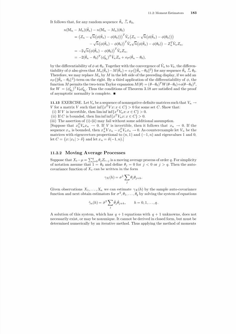
8/13/2019 van der Vaart: Time Series
http://slidepdf.com/reader/full/van-der-vaart-time-series 189/235
11.2: Moment Estimators 183
It follows that, for any random sequence θn P
→ θ0 ,
n (M n −M n )( θn ) −n(M n −M n )(θ0)
= Z n −√ n φ(θn ) −φ(θ0 ) T V n Z n −√ n φ(θn ) −φ(θ0)
−√ n φ(θn ) −φ(θ0) T V n √ n φ(θn ) −φ(θ0) −Z T n
V n Z n ,
= −2√ n φ(θn ) −φ(θ0) T V n Z n ,
= −2(˜θn −θ0)
T
(φθ0 )T ˆ
V n Z n + oP (˜θn −θ0),
by the differentiability of φ at θ0 . Together with the convergence of V n to V 0 , the differen-tiability of φ also gives that M n (θn )−M (θn ) = oP θn −θ0
2 for any sequence θn P
→θ0 .Therefore, we may replace M n by M in the left side of the preceding display, if we add anoP θn −θ0
2 -term on the right. By a third application of the differentiability of φ, thefunction M permits the two-term Taylor expansion M (θ) = ( θ−θ0 )T W (θ−θ0)+ o(θ−θ0)2 ,for W = ( φθ0
)T V 0φθ0. Thus the conditions of Theorem 3.18 are satised and the proof
of asymptotic normality is complete.
11.13 EXERCISE. Let V n be a sequence of nonnegative-denite matrices such that V n →V for a matrix V such that inf xT V x: x C > 0 for some set C . Show that:(i) If V is invertible, then lim inf inf xT V n x: x C > 0.
(ii) If C is bounded, then lim inf inf xT
V n x: x C > 0.(iii) The assertion of (i)-(ii) may fail without some additional assumption.[Suppose that xT
n V n xn → 0. If V is invertible, then it follows that xn → 0. If thesequence xn is bounded, then xT
n V xn −xT n V n xn → 0. As counterexample let V n be the
matrices with eigenvectors propertional to ( n, 1) and (−1, n) and eigenvalues 1 and 0,let C = x: |x1| > δ and let xn = δ (−1, n).]
11.2.2 Moving Average Processes
Suppose that X t −µ = qj =0 θj Z t−j is a moving average process of order q . For simplicity
of notation assume that 1 = θ0 and dene θj = 0 for j < 0 or j > q . Then the auto-covariance function of X t can be written in the form
γ X (h) = σ2
j
θj θj + h .
Given observations X 1 , . . . , X n we can estimate γ X (h) by the sample auto-covariancefunction and next obtain estimators for σ2 , θ1 , . . . , θq by solving the system of equations
γ n (h) = σ2
j
θj θj + h , h = 0 , 1, . . . , q .
A solution of this system, which has q + 1 equations with q + 1 unknowns, does notnecessarily exist, or may be nonunique. It cannot be derived in closed form, but must bedetermined numerically by an iterative method. Thus applying the method of moments
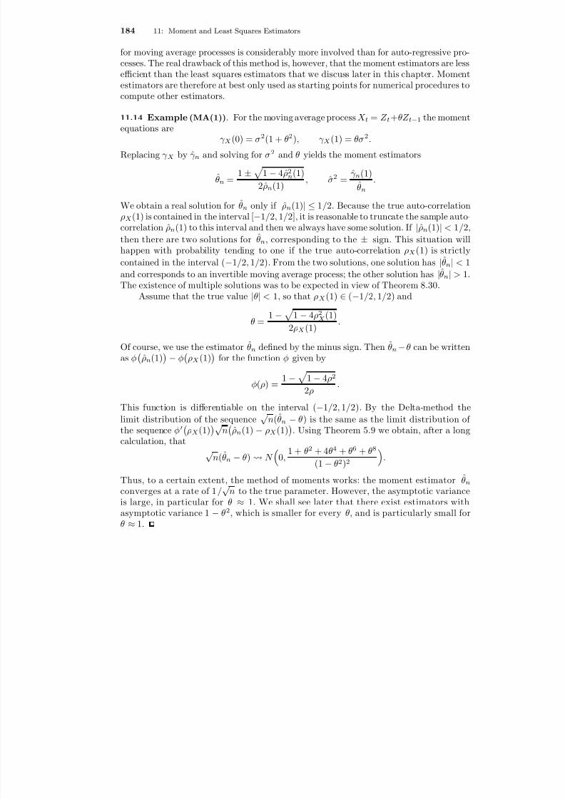
8/13/2019 van der Vaart: Time Series
http://slidepdf.com/reader/full/van-der-vaart-time-series 190/235
184 11: Moment and Least Squares Estimators
for moving average processes is considerably more involved than for auto-regressive pro-cesses. The real drawback of this method is, however, that the moment estimators are lessefficient than the least squares estimators that we discuss later in this chapter. Momentestimators are therefore at best only used as starting points for numerical procedures tocompute other estimators.
11.14 Example (MA(1)) . For the moving average process X t = Z t + θZ t−1 the momentequations are
γ X (0) = σ2(1 + θ
2), γ X (1) = θσ
2.
Replacing γ X by γ n and solving for σ2 and θ yields the moment estimators
θn = 1± 1 −4ρ2
n (1)2ρn (1)
, σ2 = γ n (1)
θn.
We obtain a real solution for θn only if |ρn (1)| ≤ 1/ 2. Because the true auto-correlationρX (1) is contained in the interval [ −1/ 2, 1/ 2], it is reasonable to truncate the sample auto-correlation ρn (1) to this interval and then we always have some solution. If |ρn (1)| < 1/ 2,then there are two solutions for θn , corresponding to the ± sign. This situation willhappen with probability tending to one if the true auto-correlation ρX (1) is strictlycontained in the interval ( −1/ 2, 1/ 2). From the two solutions, one solution has |θn | < 1and corresponds to an invertible moving average process; the other solution has
|θ
n | > 1.
The existence of multiple solutions was to be expected in view of Theorem 8.30.Assume that the true value |θ| < 1, so that ρX (1) (−1/ 2, 1/ 2) and
θ = 1− 1 −4ρ2
X (1)2ρX (1)
.
Of course, we use the estimator θn dened by the minus sign. Then θn −θ can be writtenas φ ρn (1) −φ ρX (1) for the function φ given by
φ(ρ) = 1− 1 −4ρ2
2ρ .
This function is differentiable on the interval ( −1/ 2, 1/ 2). By the Delta-method the
limit distribution of the sequence √ n(θn − θ) is the same as the limit distribution of the sequence φ ρX (1) √ n ρn (1) −ρX (1) . Using Theorem 5.9 we obtain, after a longcalculation, that
√ n(θn −θ) N 0, 1 + θ2 + 4 θ4 + θ6 + θ8
(1 −θ2 )2 .
Thus, to a certain extent, the method of moments works: the moment estimator θnconverges at a rate of 1 / √ n to the true parameter. However, the asymptotic varianceis large, in particular for θ ≈ 1. We shall see later that there exist estimators withasymptotic variance 1 − θ2 , which is smaller for every θ, and is particularly small forθ ≈1.
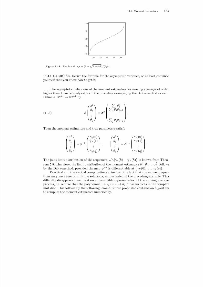
8/13/2019 van der Vaart: Time Series
http://slidepdf.com/reader/full/van-der-vaart-time-series 191/235
11.2: Moment Estimators 185
−0.4 −0.2 0.0 0.2 0.4
− 1
. 0
− 0
. 5
0 . 0
0 . 5
1 . 0
Figure 11.1. The function ρ → (1 − 1 − 4ρ2 ) / (2 ρ).
11.15 EXERCISE. Derive the formula for the asymptotic variance, or at least convinceyourself that you know how to get it.
The asymptotic behaviour of the moment estimators for moving averages of orderhigher than 1 can be analysed, as in the preceding example, by the Delta-method as well.Dene φ: R q+1
→R q+1 by
(11.4) φ
σ2
θ1...
θq
= σ2
j θ2j
j θj θj +1...
j θj θj + q
.
Then the moment estimators and true parameters satisfy
σ2
θ1...
θq
= φ−1
γ n (0)γ X (1)
...
γ n (q )
,
σ2
θ1...
θq
= φ−1
γ X (0)γ X (1)
...
γ X (q )
.
The joint limit distribution of the sequences √ n γ n (h) −γ X (h) is known from Theo-rem 5.8. Therefore, the limit distribution of the moment estimators ˆ σ2 , θ1 , . . . , θq followsby the Delta-method, provided the map φ−1 is differentiable at γ X (0), . . . , γ X (q ) .
Practical and theoretical complications arise from the fact that the moment equa-tions may have zero or multiple solutions, as illustrated in the preceding example. Thisdifficulty disappears if we insist on an invertible representation of the moving averageprocess, i.e. require that the polynomial 1 + θ1z + · · ·+ θqzq has no roots in the complexunit disc. This follows by the following lemma, whose proof also contains an algorithmto compute the moment estimators numerically.

8/13/2019 van der Vaart: Time Series
http://slidepdf.com/reader/full/van-der-vaart-time-series 192/235
186 11: Moment and Least Squares Estimators
11.16 Lemma. Let Θ R q be the set of all vectors (θ1 , . . . , θq) such that all roots of 1 + θ1 z + · · ·+ θqzq are outside the unit circle. Then the map φ: R + ×Θ →R in (11.4)is one-to-one and continuously differentiable. Furthermore, the map φ−1 is differentiable at every point φ(σ2 , θ1 , . . . , θq) for which the roots of 1 + θ1 z + · · ·+ θqzq are distinct.
* Proof. Abbreviate γ h = γ X (h). The system of equations σ2j θj θj + h = γ h for h =
0, . . . , q implies thatq
h = −qγ h zh = σ2
h jθj θj + h zh = σ2θ(z−1)θ(z).
For any h ≥ 0 the function zh + z−h can be expressed as a polynomial of degree h inw = z + z−1 . For instance, z2 + z−2 = w2 − 2 and z3 + z−3 = w3 − 3w. The caseof general h can be treated by induction, upon noting that by rearranging Newton’sbinomial formula
zh +1 + z−h −1 −wh +1 = − h + 1
(h + 1) / 2 −j =0
h + 1(h + 1 − j )/ 2
(z j + z−j ).
Thus the left side of the preceding display can be written in the form
γ 0 +
h =1
γ j (z j + z−j ) = a0 + a1w + · · ·+ aqwq ,
for certain coefficients ( a0 , . . . , a q). Let w1 , . . . , wq be the zeros of the polynomial onthe right, and for each j let ηj and η−1
j be the solutions of the quadratic equationz + z−1 = wj . Choose |ηj | ≥ 1. Then we can rewrite the right side of the precedingdisplay as
aq
q
j =1
(z + z−1 −wj ) = aq(z −ηj )(ηj −z−1)η−1j .
On comparing this to the rst display of the proof, we see that η1 , . . . , ηq are the zerosof the polynomial θ(z). This allows us to construct a map
(γ 0 , . . . , γ q) → (a0 , . . . , a q) → (w1 , . . . , wq , aq) → (η1 , . . . , ηq , aq) → (θ1 , . . . , θq , σ2).
If restricted to the range of φ this is exactly the map φ−1 . It is not hard to see that therst and last step in this decomposition of φ−1 are analytic functions. The two middlesteps concern mapping coefficients of polynomials into their zeros.
For α = ( α 0 , . . . , α q) C q+1 let pα (w) = α0 + α1w + · · ·+ αqwq . By the implicitfunction theorem for functions of several complex variables we can show the following.If for some α the polynomial pα has a root of order 1 at a point wα , then there existsneighbourhoods U α and V α of α and wα such that for every β U α the polynomial pβhas exactly one zero wβ V α and the map β → wβ is analytic on U α . Thus, under theassumption that all roots are or multiplicity one, the roots can be viewed as analyticfunctions of the coefficients. If θ has distinct roots, then η1 , . . . , ηq are of multiplicity oneand hence so are w1 , . . . , wq . In that case the map is analytic.

8/13/2019 van der Vaart: Time Series
http://slidepdf.com/reader/full/van-der-vaart-time-series 193/235
11.2: Moment Estimators 187
* 11.2.3 Moment Estimators for ARMA Processes
If X t −µ is a stationary ARMA process satisfying φ(B )(X t −µ) = θ(B )Z t , then
cov φ(B )(X t −µ), X t−k = E θ(B )Z t X t−k .
If X t −µ is a causal, stationary ARMA process, then the right side vanishes for k > q .Working out the left side, we obtain the eqations
γ X (k) −φ1γ X (k −1) −· · ·−φ pγ X (k − p) = 0 , k > q.
For k = q + 1 , . . . , q + p this leads to the system
γ X (q ) γ X (q −1) · · · γ X (q − p + 1)γ X (q + 1) γ X (q ) · · · γ X (q − p + 2)
......
...γ X (q + p −1) γ X (q + p −2) · · · γ X (q )
φ1φ2...
φ p
=
γ X (q + 1)γ X (q + 2)
...γ X (q + p)
.
These are the Yule-Walker equations for general stationary ARMA processes and may
be used to obtain estimators ˆφ1 , . . . ,
ˆφ p of the auto-regressive parameters in the sameway as for auto-regressive processes: we replace γ X by γ n and solve for φ1 , . . . , φ p .
Next we apply the method of moments for moving averages to the time se-ries Y t = θ(B )Z t to obtain estimators for the parameters σ2 , θ1 , . . . , θq . Because alsoY t = φ(B )(X t −µ) we can write the covariance function γ Y in the form
γ Y (h) =i j
φi φj γ X (h + i − j ), if φ(z) =j
φj z j .
Let γ Y (h) be the estimators obtained by replacing the unknown parameters φj = −φjand γ X (h) by their moment estimators and sample moments, respectively. Next we solveσ2 , θ1 , . . . , θq from the system of equations
γ Y (h) = σ2
j
θj θj + h , h = 0, 1, . . . , q .
As is explained in the preceding section, if X t − µ is invertible, then the solution isunique, with probability tending to one, if the coefficients θ1 , . . . , θq are restricted to givean invertible stationary ARMA process.
The resulting estimators (ˆ σ2 , θ1 , . . . , θq , φ1 , . . . , φ p) can be written as a function of γ n (0) , . . . , γ n (q + p) . The true values of the parameters can be written as the same
function of the vector γ X (0) , . . . , γ X (q + p) . In principle, under some conditions, thelimit distribution of the estimators can be obtained by the Delta-method.

8/13/2019 van der Vaart: Time Series
http://slidepdf.com/reader/full/van-der-vaart-time-series 194/235
188 11: Moment and Least Squares Estimators
* 11.2.4 Stochastic Volatility Models
In the stochastic volatility model discussed in Section 10.4 an observation X t is de-ned as X t = σt Z t for logσt a stationary auto-regressive process satisfying log σt =α + φ log σt−1 + σV t−1 , and (V t , Z t ) an i.i.d. sequence of bivariate normal vectors withmean zero, unit variances and correlation δ . Thus the model is parameterized by fourparameters α,φ,σ, δ .
The series X t is a white noise series and hence we cannot use the auto-covariances
γ X (h) at lags h = 0 to construct moment estimators. Instead, we might use highermarginal moments or auto-covariances of powers of the series. In particular, it is com-puted in Section 10.4 that
E|X t | = exp 12
σ2
1 −φ2 + α1 −φ 2π ,
E|X t |2 = exp 12
4σ2
1 −φ2 + 2α1 −φ
,
E|X t |3 = exp 12
9σ2
1 −φ2 + 3α1 −φ
2 2π ,
EX 4t = exp 8σ2
1 −φ2 + 4α1 −φ
3,
ρX 2 (1) = (1 + 4δ 2σ2)e4σ2
φ/ (1 −φ2
) −13e4σ 2 / (1 −φ 2 ) −1
,
ρX 2 (2) = (1 + 4δ 2σ2φ2)e4σ 2 φ2 / (1 −φ2 ) −1
3e4σ 2 / (1 −φ 2 ) −1 ,
ρX 2 (3) = (1 + 4δ 2σ2φ4)e4σ 2 φ3 / (1 −φ2 ) −1
3e4σ 2 / (1 −φ 2 ) −1 .
We can use a selection of these moments to dene moment estimators, or use some orall of them to dene generalized moments estimators. Because the functions on the rightside are complicated, this requires some effort, but it is feasible.
11.3 Least Squares Estimators
For auto-regressive processes the method of least squares is directly suggested by thestructural equation dening the model, but it can also be derived from the predictionproblem. The second point of view is deeper and can be applied to general time series.
A least squares estimator is based on comparing the predicted value of an observa-tion X t based on the preceding observations to the actually observed value X t . Such aprediction Π t−1X t will generally depend on the underlying parameter θ of the model,
See Taylor (1986).
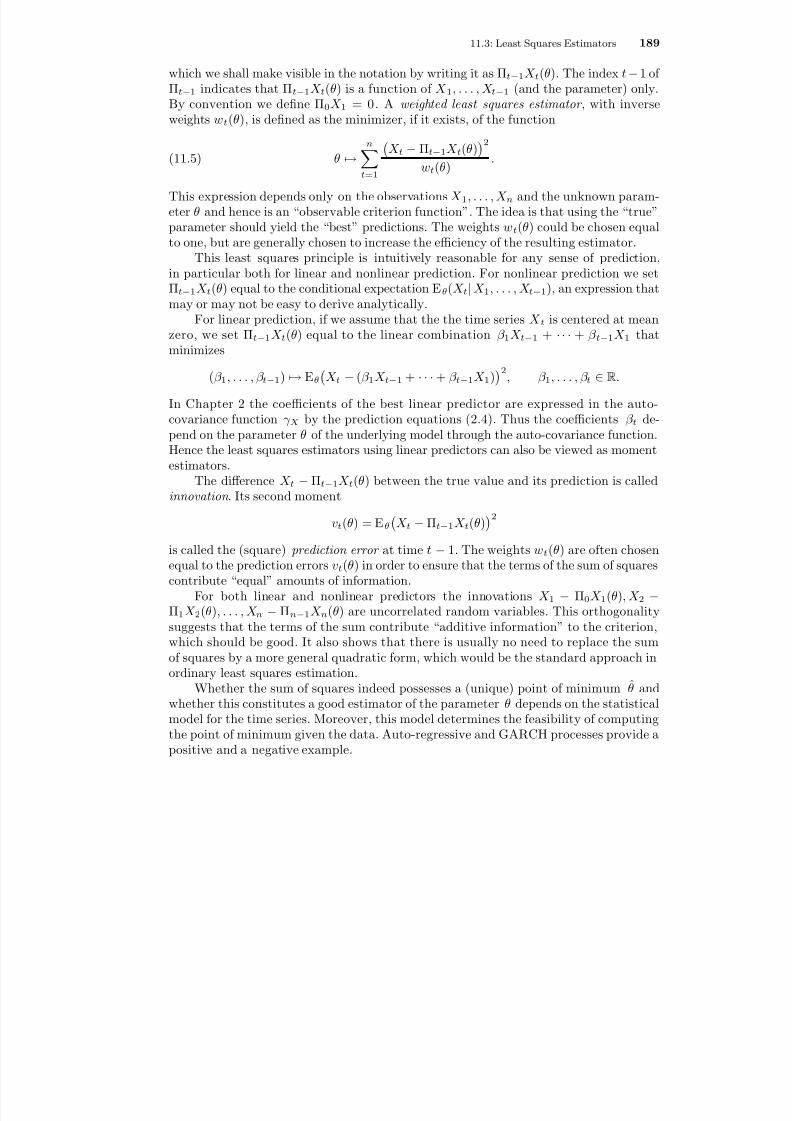
8/13/2019 van der Vaart: Time Series
http://slidepdf.com/reader/full/van-der-vaart-time-series 195/235
11.3: Least Squares Estimators 189
which we shall make visible in the notation by writing it as Π t−1X t (θ). The index t−1 of Πt−1 indicates that Π t−1X t (θ) is a function of X 1 , . . . , X t−1 (and the parameter) only.By convention we dene Π 0X 1 = 0. A weighted least squares estimator , with inverseweights wt (θ), is dened as the minimizer, if it exists, of the function
(11.5) θ →n
t =1
X t −Πt−1X t (θ) 2
wt (θ) .
This expression depends only on the observations X 1 , . . . , X n and the unknown param-eter θ and hence is an “observable criterion function”. The idea is that using the “true”parameter should yield the “best” predictions. The weights wt (θ) could be chosen equalto one, but are generally chosen to increase the efficiency of the resulting estimator.
This least squares principle is intuitively reasonable for any sense of prediction,in particular both for linear and nonlinear prediction. For nonlinear prediction we setΠt−1 X t (θ) equal to the conditional expectation E θ(X t |X 1 , . . . , X t−1), an expression thatmay or may not be easy to derive analytically.
For linear prediction, if we assume that the the time series X t is centered at meanzero, we set Πt−1 X t (θ) equal to the linear combination β 1X t−1 + ·· · + β t−1X 1 thatminimizes
(β 1 , . . . , β t−1)
→ Eθ X t
−(β 1X t−1 +
· · ·+ β t−1X 1) 2 , β 1 , . . . , β t
R .
In Chapter 2 the coefficients of the best linear predictor are expressed in the auto-covariance function γ X by the prediction equations (2.4). Thus the coefficients β t de-pend on the parameter θ of the underlying model through the auto-covariance function.Hence the least squares estimators using linear predictors can also be viewed as momentestimators.
The difference X t −Πt−1X t (θ) between the true value and its prediction is calledinnovation . Its second moment
vt (θ) = E θ X t −Πt−1 X t (θ) 2
is called the (square) prediction error at time t −1. The weights wt (θ) are often chosenequal to the prediction errors vt (θ) in order to ensure that the terms of the sum of squarescontribute “equal” amounts of information.
For both linear and nonlinear predictors the innovations X 1 − Π0X 1(θ), X 2 −Π1 X 2(θ), . . . , X n − Πn −1 X n (θ) are uncorrelated random variables. This orthogonalitysuggests that the terms of the sum contribute “additive information” to the criterion,which should be good. It also shows that there is usually no need to replace the sumof squares by a more general quadratic form, which would be the standard approach inordinary least squares estimation.
Whether the sum of squares indeed possesses a (unique) point of minimum θ andwhether this constitutes a good estimator of the parameter θ depends on the statisticalmodel for the time series. Moreover, this model determines the feasibility of computingthe point of minimum given the data. Auto-regressive and GARCH processes provide apositive and a negative example.

8/13/2019 van der Vaart: Time Series
http://slidepdf.com/reader/full/van-der-vaart-time-series 196/235
190 11: Moment and Least Squares Estimators
11.17 Example (Autoregression) . A mean-zero, causal, stationary, auto-regressiveprocess of order p is modelled through the parameter θ = ( σ2 , φ1 , . . . , φ p). For t ≥ p thebest linear predictor is given by Π t−1X t = φ1X t−1 + · · ·φ pX t− p and the prediction erroris vt = E Z 2t = σ2 . For t < p the formulas are more complicated, but could be obtainedin principle.
The weighted sum of squares with weights wt = vt reduces to
p
t =1
X t −Πt−1X t (φ1 , . . . , φ p) 2
vt (σ2 , φ1 , . . . , φ p) +
n
t = p+1
X t −φ1 X t−1 − · · ·−φ pX t− p2
σ2 .
Because the rst term, consisting of p of the n terms of the sum of squares, possesses acomplicated form, it is often dropped from the sum of squares. Then we obtain exactlythe sum of squares considered in Section 11.1, but with X n replaced by 0 and divided byσ2 . For large n the difference between the sums of squares and hence between the twotypes of least squares estimators should be negligible.
Another popular strategy to simplify the sum of squares is to act as if the “ob-servations” X 0 , X −1 , . . . , X − p+1 are available and to redene Π t−1X t for t = 1, . . . , paccordingly. This is equivalent to dropping the rst term and letting the sum in thesecond term start at t = 1 rather than at t = p + 1. To implement the estimator we mustnow choose numerical values for the missing observations X 0 , X −1 , . . . , X − p+1 ; zero is acommon choice.
The least squares estimators for φ1 , . . . , φ p, being (almost) identical to the Yule-Walker estimators, are √ n-consistent and asymptotically normal. However, the leastsquares criterion does not lead to a useful estimator for σ2 : minimization over σ2 leadsto σ2 = ∞ and this is obviously not a good estimator. A more honest conclusion is thatthe least squares criterion as posed originally fails for auto-regressive processes, sinceminimization over the full parameter θ = ( σ2 , φ1 , . . . , φ p) leads to a zero sum of squaresfor σ2 = ∞ and arbitrary (nite) values of the remaining parameters. The method of least squares works only for the subparameter ( φ1 , . . . , φ p) if we rst drop σ2 from thesum of squares.
11.18 Example (GARCH) . A GARCH process is a martingale difference series andhence the one-step predictions Π t−1X t (θ) are identically zero. Consequently, the weighted
least squares sum, with weights equal to the prediction errors, reduces ton
t =1
X 2tvt (θ)
.
Minimizing this criterion over θ is equivalent to maximizing the prediction errors vt (θ).It is intuitively clear that this does not lead to reasonable estimators.
One alternative is to apply the least squares method to the squared series X 2t . Thissatises an ARMA equation in view of (9.3). (Note however that the innovations in thatequation are also dependent on the parameter.)
The best x of the least squares method is to augment the least squares criterion tothe Gaussian likelihood, as discussed in Chapter 13.
8/13/2019 van der Vaart: Time Series
http://slidepdf.com/reader/full/van-der-vaart-time-series 197/235
11.3: Least Squares Estimators 191
So far the discussion in this section has assumed implicitly that the mean valueµ = E X t of the time series is zero. If this is not the case, then we apply the precedingdiscussion to the time series X t −µ instead of to X t , assuming rst that µ is known.Then the parameter µ will show up in the least squares criterion. To dene estimators wecan either replace the unknown value µ by the sample mean X n and minimize the sumof squares with respect to the remaining parameters, or perform a joint minimizationover all parameters.
Least squares estimators can rarely be written in closed form, the case of stationary
auto-regressive processes being an exception, but iterative algorithms for the approxi-mate calculation are implemented in many computer packages. Newton-type algorithmsprovide one possibility. The best linear predictions Π t−1X t are often computed recur-sively in t (for a grid of values θ), for instance with the help of a state space representationof the time series and the Kalman lter.
The method of least squares is closely related to Gaussian likelihood, as discussed inChapter 13. Gaussian likelihood is perhaps more fundamental than the method of leastsquares. For this reason we restrict further discussion of the method of least squares toARMA processes.
11.3.1 ARMA ProcessesThe method of least squares works well for estimating the regression and moving averageparameters ( φ1 , . . . , φ p, θ1 , . . . , θq) of ARMA processes, if we perform the minimizationfor a xed value of the parameter σ2 . In general, if some parameter, such as σ2 forARMA processes, enters the covariance function as a multiplicative factor, then the bestlinear predictor Π t X t +1 is free from this parameter, by the prediction equations (2.4). Onthe other hand, the prediction error vt +1 = γ X (0) −(β 1 , . . . , β t )Γ t (β 1 , . . . , β t )T (whereβ 1 , . . . , β t are the coefficients of the best linear predictor) contains such a parameter asa multiplicative factor. It follows that the inverse of the parameter will enter the leastsquares criterion as a multiplicative factor. Thus on the one hand the least squares meth-ods does not yield an estimator for this parameter; on the other hand, we can just omitthe parameter and minimize the criterion over the remaining parameters. In particular,in the case of ARMA processes the least squares estimators for ( φ1 , . . . , φ p, θ1 , . . . , θq)are dened as the minimizers of, for ˜vt = σ−2 vt ,
n
t =1
X t
−Πt
−1X t (φ1 , . . . , φ p , θ1 , . . . , θq) 2
vt (φ1 , . . . , φ p, θ1 , . . . , θq) .
This is a complicated function of the parameters. However, for a xed value of (φ1 , . . . , φ p, θ1 , . . . , θq) it can be computed using the state space representation of anARMA process and the Kalman lter. A grid search or iteration method can do the rest.
11.19 Theorem. Let X t be a causal and invertible stationary ARMA ( p, q ) process rela-tive to an i.i.d. sequence Z t with nite fourth moments. Then the least squares estimators satisfy
√ n φ p
θq−
φ p θq
N (0, σ2J −1 φp , θq
),
8/13/2019 van der Vaart: Time Series
http://slidepdf.com/reader/full/van-der-vaart-time-series 198/235
192 11: Moment and Least Squares Estimators
where J φp , θqis the covariance matrix of (U −1 , . . . , U − p, V −1 , . . . , V −q) for stationary auto-
regressive processes U t and V t satisfying φ(B )U t = θ(B )V t = Z t .
Proof. The proof of this theorem is long and technical. See e.g. Brockwell andDavis (1991), pages 375–396, Theorem 10.8.2.
11.20 Example (MA(1)) . The least squares estimator θn for θ in the moving averageprocess X t = Z t + θZ t
−1 with
|θ
| < 1 possesses asymptotic variance equal to σ2/ var V
−1 ,
where V t is the stationary solution to the equation θ(B )V t = Z t . Note that V t is an auto-regressive process of order 1, not a moving average!
As we have seen before the process V t possesses the representation V t = ∞j =0 θj Z t−j
and hence var V t = σ2 / (1 −θ2) for every t .Thus the sequence √ n(θn −θ) is asymptotically normally distributed with mean zero
and variance equal to 1 −θ2 . This should be compared to the asymptotic distribution of the moment estimator, obtained in Example 11.14.
11.21 EXERCISE. Find the asymptotic covariance matrix of the sequence √ n(φn −φ, θn −θ) for (φn , θn ) the least squares estimators for the stationary, causal, invertibleARMA process satisfying X t = φX t−1 + Z t + θZ t−1 .

8/13/2019 van der Vaart: Time Series
http://slidepdf.com/reader/full/van-der-vaart-time-series 199/235
12Spectral Estimation
In this chapter we study nonparametric estimators of the spectral density and spectraldistribution of a stationary time series. As in Chapter 5 “nonparametric” means that noa-priori structure of the series is assumed, apart from stationarity.
If a well-tting model is available, then an alternative to the methods of this chapterare spectral estimators suited to this model. For instance, the spectral density of astationary ARMA process can be expressed in the parameters σ2 , φ1 , . . . φ p , θ1 , . . . , θq of the model (see Section 8.5) and hence can be estimated by plugging in estimators forthe parameters. If the ARMA model is appropriate, this should lead to better estimatorsthan the nonparametric estimators discussed in this chapter. We do not further discussthis type of estimator.
Let the observations X 1 , . . . , X n be the values at times 1 , . . . , n of a stationary timeseries X t , and let γ n be their sample auto-covariance function. In view of the denitionof the spectral density f X (λ), a natural estimator is
(12.1) f n,r (λ) = 12π
|h |<r
γ n (h)e−ihλ .
Whereas f X (λ) is dened as an innite series, the estimator f n,r is truncated at its r thterm. Because the estimators ˆ γ n (h) are dened only for
|h
| < n and there is no hope of
estimating the auto-covariances γ X (h) for lags |h| ≥ n , we must choose r ≤ n . Becausethe estimators ˆγ n (h) are unreliable for |h| ≈ n, it may be wise to choose r much smallerthan n . We shall see that a good choice of r depends on the smoothness of the spectraldensity and also on which aspect of the spectrum is of interest. For estimating f X (λ)at a point, values of r such as nα for some α (0, 1) may be appropriate, whereas forestimating the spectral distribution function (i.e. areas under f X ) the choice r = n workswell.
In any case, since the covariances of lags |h| ≥ n can never be estimated fromthe data, nonparametric estimation of the spectrum is hopeless, unless one is willing toassume that expressions such as |h |≥n γ X (h) are small. In Section 12.3 ahead we relatethis tail series to the smoothness of the spectral density λ → f X (λ). If this function is
8/13/2019 van der Vaart: Time Series
http://slidepdf.com/reader/full/van-der-vaart-time-series 200/235
194 12: Spectral Estimation
several times differentiable, then the auto-covariance function decreases fast to zero, andnonparametric estimation is feasible.
12.1 Finite Fourier TransformThe nite Fourier transform is a useful tool in spectral analysis, both for theory and prac-tice. The practical use comes from the fact that it can be computed efficiently by a cleveralgorithm, the Fast Fourier Transform (FFT). While a naive computation would requireO(n2 ) multiplications and summations, the FFT needs only O(n log n) operations. †
The nite Fourier transform of an arbitrary sequence x1 , . . . , x n of complex numbersis dened as the function λ → dx (λ) given by
dx (λ) = 1√ n
n
t =1xt e−iλt , λ (−π, π ].
In other words, the function n/ 2π dx (λ) is the Fourier series corresponding to thecoefficients . . . , 0, 0, x1, x2 , . . . , x n , 0, 0, . . .. The inversion formula (or a short calculation)shows that
x t =√ n2π
π
−πeitλ dx (λ) dλ, t = 1, 2, . . . , n .
Thus there is a one-to-one relationship between the numbers x1 , . . . , xn and the functiondx . We may view the function dx as “encoding” the numbers x1 , . . . , x n .
Encoding n numbers by a function on the interval ( −π, π ] is rather inefficient. Atcloser inspection the numbers x1 , . . . , x n can also be recovered from the values of dx onthe grid
. . . , −4πn
,−2πn
, 0, 2πn
, 4π
n , . . . (−π, π ].
These n points are called the natural frequencies at time n. (The value 0 is always anatural frequency; for odd n there are ( n−1)/ 2 positive and negative natural frequencies,situated symmetrically about 0; for even n the value π is a natural frequency, and theremaining natural frequencies are n/ 2 −1 points in (0 , π) and their reections.)
12.1 Lemma. If dx is the nite Fourier transform of x1 , . . . , x n C , then
x t = 1√ n j
dx (λ j )eitλ j , t = 1, 2, . . . , n ,
where the sum is computed over the natural frequencies λ j (−π, π ] at time n .
Proof. For every of the natural frequencies λ j dene a vector
ej = 1√ n (eiλ j , ei 2λ j , . . . , e inλ j )T .
† See e.g. Brockwell and Davis, Chapter 10 for a discussion.

8/13/2019 van der Vaart: Time Series
http://slidepdf.com/reader/full/van-der-vaart-time-series 201/235

8/13/2019 van der Vaart: Time Series
http://slidepdf.com/reader/full/van-der-vaart-time-series 202/235
196 12: Spectral Estimation
For natural frequencies λ j = 0 we have that d−µ1 (λ j ) = 0 for every µ, in particular forµ = X n . This implies that I n,X (λ j ) = I n,X −X n
(λ j ) and hence
(12.3) I n (λ j ) = 12π
|h |<n
γ n (h)e−ihλ , λj 2π
n Z −0.
This is exactly the estimator f n,n (λ) given in (12.1), with r = n. As noted before, weshould expect this estimator to be unreliable as an estimator of f X (λ), because of theimprecision of the estimators ˆγ n (h) for lags |h| close to n .
Under the assumption that the time series X t is stationary, we can compute themean of the periodogram, for λ = 0, as
EI n (λ) = 12π
E dX (λ) 2 = 12π
var dX (λ) + 12π
EdX (λ) 2
= 12πn
n
s =1
n
t =1cov(X s , X t )eiλ (s−t ) +
12πn
n
t =1EX t e−iλt
2
= 12π
|h |<n
1 − |h|n
γ X (h)e−iλh + µ2
2πn1 −e−iλn
1 −e−iλ
2
.
The second term on the far right is of the order O(1/n ) for every λ
= 0 (and λ
(−π, π )) and even vanishes for every natural frequency λj = 0. Under the conditionthat h γ X (h) < ∞, the rst term converges to f X (λ) as n → ∞, by the dominatedconvergence theorem. We conclude that the periodogram is asymptotically unbiased forestimating the spectral density, in that E I n (λ) → f X (λ). This is a good property.
However, the periodogram is not a consistent estimator for f X (λ): the followingtheorem shows that I n (λ) is asymptotically exponentially distributed with mean f X (λ),whence we do not have that I n (λ) P
→ f X (λ). Using the periodogram as an estimator of f X (λ) is asymptotically equivalent to estimating f X (λ) using a single observation froman exponential distribution with mean f X (λ). This is disappointing, because we shouldhope that after observing the time series X t long enough, we are able to estimate itsspectral density with arbitrary precision. The periodogram does not fulll this hope, asit keeps uctuating around the target value f X (λ). Apparently, it does not effectivelyuse the information available in the observations X 1 , . . . , X n .
12.4 Theorem. Let X t = ψj Z t−j for an i.i.d. sequence Z t with mean zero and nite second moment and coefficients ψj with j |ψj | < ∞. Then for any values 0 < µ 1 < ·· · <µk < π the variables I n (µ1), . . . , I n (µk ) are asymptotically distributed as independentexponential variables with means f X (µ1), . . . , f X (µk ), respectively.
Proof. First consider the case that X t = Z t for every t. Then the spectral density f X (λ)is the function f Z (λ) = σ2 / 2π, for σ2 the variance of the white noise sequence. We canwrite
dZ (λ) = 1√ n
n
t =1Z t cos(λt ) −i
1√ n
n
t =1Z t sin(λt ) =: An (λ) −iB n (λ).

8/13/2019 van der Vaart: Time Series
http://slidepdf.com/reader/full/van-der-vaart-time-series 203/235
12.2: Periodogram 197
By straightforward calculus we nd that, for any λ, µ (0, π),
cov An (λ), An (µ) = σ2
n
n
t =1cos(λt )cos(µt) →
σ2 / 2 if λ = µ,0 if λ = µ,
cov Bn (λ), Bn (µ) = σ2
n
n
t =1sin(λt )sin( µt) → σ2 / 2 if λ = µ,
0 if λ = µ,
cov An (λ), Bn (µ) = σ2
n
n
t =1 cos(λt )sin( µt) → 0.
By the Lindeberg central limit theorem, Theorem 3.16, we now nd that the se-quence of vectors An (λ), Bn (λ), An (µ), Bn (µ) converges in distribution to a vector(G1 , G2 , G3 , G4) with the N 4 0, (σ2 / 2)I distribution. Consequently, by the continuousmapping theorem,
I n (λ), I n (µ) = 12π
A2n (λ) + B 2
n (λ), A2n (µ) + B 2
n (µ)1
2π(G2
1 + G22 , G2
3 + G24 ).
The vector on the right is distributed as σ2/ (4π) times a vector of two independent χ 22
variables. Because the chisquare distribution with two degrees of freedom is identical tothe standard exponential distribution with parameter 1 / 2, this is the same as a vectorof two independent exponential variables with means σ2 / (2π).
This concludes the proof in the special case that X t = Z t and for two frequencies λand µ. The case of k different frequencies µ1 , . . . , µk can be treated in exactly the sameway, but is notationally more involved.
The spectral density of a general time series of the form X t = j ψj Z t−j satisesf X (λ) = ψ(λ) 2f Z (λ), for ψ(λ) = ψj e−ijλ the transfer function of the linear lter. Weshall prove the theorem by showing that the periodograms I n,X and I n,Z approximatelysatisfy a similar relation. Indeed, rearranging sums we nd
dX (λ) = 1√ n
n
t =1 j
ψj Z t−j e−itλ =j
ψj e−ijλ 1√ n
n −j
s =1 −j
Z s e−isλ .
If we replace the sum n −js =1 −j in the right side by the sum
ns =1 , then the right side
of the display becomes ψ(λ)dZ (λ). These two sums differ by 2( | j | n) terms, every of
the terms Z s e−iλs
having mean zero and variance bounded by σ2, and the terms beingindependent. Thus
E1
√ nn −j
s =1 −j
Z s e−isλ −dZ (λ)2
≤2 | j | nn
σ2 .
In view of the inequality E |X | ≤ EX 2 1/ 2 , we can drop the square on the left side if wetake a root on the right side. Next combining the two preceding displays and applyingthe triangle inequality, we nd
E dX (λ) −ψ(λ)dZ (λ) ≤j
|ψj | 2 | j | nn
1/ 2σ.

8/13/2019 van der Vaart: Time Series
http://slidepdf.com/reader/full/van-der-vaart-time-series 204/235
198 12: Spectral Estimation
The j th term of the series is bounded by |ψj | 2| j |/n1/ 2 σ and hence converges to zero
as n → ∞, for every xed j ; it is also dominated by |ψj |√ 2σ. Therefore, the right sideof preceding display converges to zero as n → ∞.By Markov’s and Slutsky’s lemmas it follows that dX (λ) has the same limit dis-tribution as ψ(λ)dZ (λ). Hence, by the continuous mapping theorem, the sequenceI n,X (λ) has the same limit distribution as |ψ(λ)|2 I n,Z (λ). This is true for every xedλ, but also for nite sets of λ jointly. The proof is nished, because the variables
|ψ(λ)
|2 I n,Z (λ) are asymptotically distributed as independent exponential variables with
means |ψ(λ)|2 f Z (λ), by the rst part of the proof.
A remarkable aspect of the preceding theorem is that the periodogram values I n (λ)at different frequencies are asymptotically independent. This is well visible already fornite values of n in plots of the periodogram, which typically have a wild and peakyappearance. The theorem says that for large n such a plot should be similar to a plotof independent exponentially distributed variables E λ with means f X (λ) (on the y-axis)versus λ (on the x-axis).
0.0 0.1 0.2 0.3 0.4 0.5
- 3 0
- 2 0
- 1 0
0
1 0
frequency
s p e c
t r u m
Figure 12.1. Periodogram of a realization of the moving average X t = 0 .5Z t + 0 .2Z t − 1 + 0 .5Z t − 2 for aGaussian white noise series. (Vertical scale in decibel, i.e. 10 log.)
The following theorem shows that we even have independence of the periodogramvalues at natural frequencies that converge to the same value.
8/13/2019 van der Vaart: Time Series
http://slidepdf.com/reader/full/van-der-vaart-time-series 205/235
12.2: Periodogram 199
12.5 Theorem. Let X t = ψj Z t−j for an i.i.d. sequence Z t with nite second moments and coefficients ψj with j |ψj | < ∞. Let λn = (2 π/n ) jn for jn Z be a sequence of natural frequencies such that λn → λ (0, π). Then for any k Z the variables I n (λn −k2π/n ), I n λn −(k−1)2π/n , . . . , I n (λn + k2π/n ) are asymptotically distributed as independent exponential variables with mean f X (λ).
Proof. The second part of the proof of Theorem 12.4 is valid uniformly in λ and henceapplies to sequences of frequencies λn . For instance, the continuity of ψ(λ) and the proof shows that dX (µn ) −ψ(µn )dZ (µn ) P→ 0 for any sequence µn . It suffices to extend therst part of the proof, which concerns the special case that X t = Z t .
Here we apply the same method as in the proof of Theorem 12.4. The limits of the covariances are as before, where in the present case we use the fact that we areconsidering natural frequencies only. For instance,
cov An k2πn
, Bn l2πn
= σ2
2
n
t =1cos kt
2πn
sin lt2πn
= 0 ,
for every integers k, l such that ( k + l)/n and (k − l)/n are not contained in Z . Anapplication of the Lindeberg central limit theorem concludes the proof.
The sequences of frequencies λn + j (2π/n ) considered in the preceding theorem allconverge to the same value λ . That Theorem 12.4 remains valid (it does) if we replacethe xed frequencies µj in this theorem by sequences µj,n → µj is not very surprising.More surprising is the asymptotic independence of the periodograms I n (µn,j ) even if every sequence µn,j converges to the same frequency λ. As the proof of the precedingtheorem shows, this depends crucially on using natural frequencies µn,j .
The remarkable independence of the periodogram at frequencies that are very closetogether is a further explanation of the peaky appearance of the periodogram I n (λ) asa function of λ. It is clear that this function is not a good estimator of the spectraldensity. However, the independence suggests ways of improving our estimator for f X (λ).The values I n (λn −k2π/n ), I n λn −(k −1)2π/n , . . . , I n (λn + k2π/n ) can be viewed asa sample of independent estimators of f X (λ), for any k. Rather than one exponentiallydistributed veriable, we therefore have many exponentially distributed variables, all withthe same (asymptotic) mean. We exploit this in the next section.
In practice the periodogram may have one or a few extremely high peaks thatcompletely dominate its graph. This indicates an important cyclic component in the timeseries at those frequencies. Cyclic components of smaller amplitude at other frequenciesmay be hidden. It is practical wisdom that in such a case a fruitful spectral analysis atother frequencies requires that the peak frequencies are rst removed from the signal(by a lter with the appropriate transfer function). We next estimate the spectrum of the new time series and, if desired, transform this back to obtain the spectrum of theoriginal series, using the formula given in Theorem 6.10. Because a spectrum withouthigh peaks is similar to the uniform spectrum of a white noise series, this procedure isknown as prewhitening of the data.
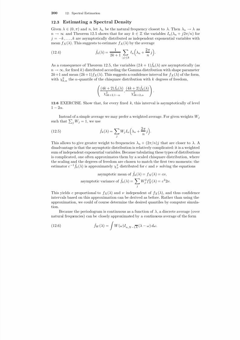
8/13/2019 van der Vaart: Time Series
http://slidepdf.com/reader/full/van-der-vaart-time-series 206/235
8/13/2019 van der Vaart: Time Series
http://slidepdf.com/reader/full/van-der-vaart-time-series 207/235
8/13/2019 van der Vaart: Time Series
http://slidepdf.com/reader/full/van-der-vaart-time-series 208/235
202 12: Spectral Estimation
from Fourier analysis, where convergence factors were introduced to improve the ap-proximation properties of a Fourier series: it was noted that for suitably chosen weightsw(h) the partial sums |h |<n w(h)γ X (h)e−ihλ could be much closer to the full series
h γ X (h)e−ihλ than the same partial sums with w ≡1. In our statistical context this iseven more so the case, because we introduce additional approximation error by replacingthe coefficients γ X (h) by the estimators ˆγ n (h).
12.7 Example. The tapering function
w(h) = 0 if |h| ≤ r ,1 if |h| > r ,
corresponds to the Dirichlet kernel
W (λ) = 12π
|h |≤r
e−ihλ = 12π
sin(r + 12 )λ
sin 12 λ
.
Therefore, the estimator (12.1) should be compared to the estimators (12.5) and (12.6)with weights W j chosen according to the Dirichlet kernel.
12.8 Example. The uniform kernel
W (λ) = r/ (2π) if |λ| ≤ π/r ,0 if |λ| > π/r ,
corresponds to the weight function w(h) = r sin(πh/r )/ (πh ). These choices of spectraland lag windows correspond to the estimator (12.4).
All estimators for the spectral density considered so far can be viewed as smoothed periodograms : the value f (λ) of the estimator at λ is an average or weighted average of values I n (µ) for µ in a neighbourhood of λ. Thus “irregularities” in the periodogramare “smoothed out”. The amount of smoothing is crucial for the accuracy of the estima-tors. This amount, called the bandwidth , is determined by the parameter k in (12.4), theweights W j in (12.5), the kernel W in (12.6), and, more hidden, by the parameter r in(12.1). For instance, a large value of k in (12.4) or a kernel W with a large variance in(12.6) result in a large amount of smoothing (large bandwidth). Oversmoothing , choos-ing a bandwidth that is too large, results in spectral estimators that are too at andtherefore inaccurate, whereas undersmoothing , choosing too small a bandwidth, yieldsspectral estimators that share the bad properties of the periodogram. In practice an “op-timal” bandwidth is often determined by plotting the spectral estimators for a number of different bandwidths and next choosing the one that looks “reasonable”. An alternativeis to use one of several methods of “data-driven” choices of bandwidths, such as crossvalidation or penalization. We omit a discussion.
Theoretical analysis of the choice of the bandwidth is almost exclusively asymp-totical in nature. Given a number of observations tending to innity, the “optimal”bandwidth decreases to zero. A main concern of an asymptotic analysis is to determine

8/13/2019 van der Vaart: Time Series
http://slidepdf.com/reader/full/van-der-vaart-time-series 209/235
12.3: Estimating a Spectral Density 203
the rate at which the bandwidth should decrease as the number of observations tendsto innity. The key concept is the bias-variance trade-off . Because the periodogram ismore or less unbiased, little smoothing gives an estimator with small bias. However, aswe have seen, the estimator will have a large variance. Oversmoothing has the oppositeeffects. Because accurate estimation requires that both bias and variance are small, weneed an intermediate value of the bandwidth.
We shall quantify this bias-variance trade-off for estimators of the type (12.1), wherewe consider r as the bandwidth parameter. As our objective we take to minimize the
mean integrated square error
(12.7) 2π E π
−πf n,r (λ) −f X (λ) 2 dλ.
The integrated square error is a global measure of the discrepancy between f n,r andf X . Because we are interested in f X as a function, it is more relevant than the distancef n,r (λ) −f X (λ) for any xed λ.
We shall use Parseval’s identity, which says that the space L2(−π, π ] is isometric tothe space 2 .
12.9 Lemma (Parseval’s identity) . Let f : (−π, π ] →C be a measurable function suchthat
|f |2(λ) dλ < ∞. Then its Fourier coefficients f j =
π
−π eijλ f (λ) dλ satisfy
π
−πf (λ) 2 dλ =
12π
∞
j = −∞|f j |2 .
12.10 EXERCISE. Prove this identity. Also show that for a pair of square-integrable,measurable functions f , g : (−π, π ] →C we have f (λ)g(λ) dλ = j f j gj .
The function f n,r −f X possesses the Fourier coefficients ˆγ n (h) −γ X (h) for |h| < rand −γ X (h) for |h| ≥ r . Thus, Parseval’s identity yields that the mean integrated squareerror (12.7) is equal to
E
|h
|<r
γ n (h) −γ X (h) 2 +
|h
|≥r
γ X (h) 2
In a rough sense the two terms in this formula are the “variance” and the square “bias”term. A large value of r clearly decreases the second, square bias term, but increases therst, variance term. This variance term can itself be split into a bias and variance termand we can reexpress the mean integrated square error as
|h |<r
var γ n (h) +
|h |<r
Eγ n (h) −γ X (h) 2 +
|h |≥r
γ X (h) 2 .
Assume for simplicity that E X t = 0 and that X t = j ψj Z t−j for a summable sequence(ψj ) and i.i.d. sequence Z t with nite fourth moments. Furthermore, assume that we usethe estimator ˆγ n (h) = n−1 n −h
t =1 X t + h X t rather than the true sample auto-covariance

8/13/2019 van der Vaart: Time Series
http://slidepdf.com/reader/full/van-der-vaart-time-series 210/235
204 12: Spectral Estimation
function. (The results for the general case are similar, but the calculations will be moreinvolved. Note that the difference between the present estimator and the usual one isapproximately X and |h |<r E(X )4 = O(r/n 2), under appropriate moment conditions.This is negligible in the following.) Then the calculations in Chapter 5 show that thepreceding display is equal to
|h
|<r
1n2
|g
|<n
−|h
|
n − |h| − |g| κ4σ4
i
ψi ψi + h ψi+ g ψi + g+ h + γ 2X (g)
+ γ X (g + h)γ X (g −h) +
|h |<r
|h|n
γ X (h)2
+
|h |≥r
γ 2X (h)
≤ |κ4|σ4
nh g i
|ψi ψi+ h ψi+ g ψi+ g+ h |+ 2rn g
γ 2X (g)
+ 1n
h gγ X (g + h)γ X (g −h) +
r2
n 2h
γ 2X (h) +
|h |≥r
γ 2X (h).
To ensure that the second and last terms on the right converge to zero as n → ∞ wemust choose r = r n such that r n /n → 0 and r n → ∞, respectively. The rst and thirdterm are of the order O(1/n ), and the fourth term is of the order O(r 2
n /n 2). Under therequirements rn
→ ∞ and rn /n
→ 0 these terms are dominated by the other terms, and
the whole expression is of the orderrn
n +
|h |≥r n
γ 2X (h).
A rst conclusion is that the sequence of estimators f n,r n is asymptotically consistentfor estimating f X relative to the L2-distance whenever rn → ∞ and r n /n → 0. A widerange of sequences rn satises these constraints. For an optimal choice we must makeassumptions regarding the rate at which the bias term |h |≥r γ 2X (h) converges to zeroas r → ∞. For any constant m we have that
r n
n +
|h
|≥r n
γ X (h)2 ≤ rn
n +
1r 2m
n h
γ 2X (h)h2m .
Suppose that the series on the far right converges; this means roughly that the auto-covariances γ X (h) decrease faster than |h|−m −1/ 2 as |h| → ∞. Then we can make abias-variance trade-off by balancing the terms rn /n and 1/r 2m
n . These terms are of equalorder for r n n1/ (2 m +1) ; for this choice of r n we nd that
E π
−πf n,r n (λ) −f X (λ) 2 dλ = O
1n
2m/ (2 m +1).
Large values of m yield the fastest rates of convergence. The rate n−m/ (2 m +1) is alwaysslower than n−1/ 2 , the rate obtained when using parametric spectral estimators, butapproaches this rate as m → ∞.
8/13/2019 van der Vaart: Time Series
http://slidepdf.com/reader/full/van-der-vaart-time-series 211/235
12.4: Estimating a Spectral Distribution 205
Unfortunately, in practice we do not know γ X (h) and therefore cannot check whetherthe preceding derivation is valid. So-called cross-validation techniques may be used todetermine a suitable constant m from the data.
The condition that h γ 2X (h)h2m < ∞ can be interpreted in terms of the smooth-ness of the spectral density. It can be shown (see Exercise 12.11) that the Fourier coef-cients of the mth derivative f (m )
X of f X are equal to γ X (h)(−ih )m . Consequently, byParseval’s identity
h γ 2
X (h)h2m
= π
−π f (m )
X (λ)2
dλ.Thus the left side is nite if and only if the mth derivative of f X exists and is square-integrable. Thus for time series with such an m-smooth spectral density, one can estimatethe spectral density with an integrated square error of order O(n−2m/ (2 m +1) ). This rateis uniform over the set of all time series with spectral densities such that f
(m )X (λ)2 dλ
is uniformly bounded, i.e. balls in the Sobolev space of order m.
12.11 EXERCISE. Show that the Fourier coefficients π
−π eijλ f (λ) dλ of the derivativeof a continuously differentiable function f : [−π, π ] → R with f (−π) = f (π), are equal to
−ijf j , for f j the Fourier coefficients of f . [Hint: apply partial integration.]
This conclusion is similar to the conclusion in the problem of estimating a density
given a random sample from this density, where also m-smooth densities can be estimatedwith an integrated square error of order O(n−2m/ (2 m +1) ). The smoothing methods dis-cussed previously (the estimator (12.6) in particular) are also related to the method of kernel smoothing for density estimation. It is interesting that historically the method of smoothing was rst applied to the problem of estimating a spectral density. Here kernelsmoothing of the periodogram was a natural extension of taking simple averages as in(12.4), which itself is motivated by the independence property of the periodogram. Themethod of kernel smoothing for the problem of density estimation based on a randomsample from this density was invented later, even though this problem by itself appearsto be simpler.
* 12.4 Estimating a Spectral Distribution
In the preceding section it is seen that nonparametric estimation of a spectral densityrequires smoothing and yields rates of convergence n−α for values of α < 1/ 2. In contrast,a spectral distribution function can be estimated at the “usual” rate of convergencen−1/ 2 and natural estimators are asymptotically normally distributed. We assume X t isa stationary time series with spectral density f X .
The spectral distribution function F X (λ0) = λ 0
−π f X (λ) can be written in the form
π
−πa(λ)f X (λ) dλ
8/13/2019 van der Vaart: Time Series
http://slidepdf.com/reader/full/van-der-vaart-time-series 212/235
8/13/2019 van der Vaart: Time Series
http://slidepdf.com/reader/full/van-der-vaart-time-series 213/235
12.4: Estimating a Spectral Distribution 207
the preceding argument to X n,m : = √ n am (I n −f X ) dλ) to see that X n,m N (0, σ2m )
as n → ∞, for every xed m. The asymptotic variance σ2m is the expression given in the
theorem with am instead of a. If m → ∞, then σ2m converges to the expression in the
theorem, by the dominated convergence theorem, because a is squared-integrable andf X is uniformly bounded. Therefore, by Lemma 3.10 it suffices to show that for everymn → ∞(12.9) √ n
(a −am n )(I n −f X ) dλ P
→ 0.
Set b = a−am n . The variance of the random variable in (12.9) is the same as the varianceof (a −am n )I n dλ, and can be computed as, in view of Parseval’s identity,
var√ n2π
|h |<n
γ n (h)bh = n4π2
|g|<n |h |<n
cov γ n (g), γ n (h) bg bh
= n4π2
|g|<n |h |<n
1n2
n −|g|
s =1
n −|h |
t =1cov(X s + g X s , X t + h X t )bg bh .
Using the same approach as in Section 5.2, we can rewrite this as
14π2n
|g|<n |h |<n
n −|g|
s =1
n −|h |
t =1
κ4σ4
i
ψi+ g ψi ψt−s + h + i ψt−s + i
+ γ X (t −s + h −g)γ X (t −s) + γ X (t −s −g)γ X (t −s + h) bg bh .
The absolute value of this expression can be bounded above by1
4π2g h k i
|ψi+ g ψi ψk+ h + i ψk+ i ||κ4|σ4 + γ X (k + h −g)γ X (k)
+ γ X (k −g)γ X (k + h) |bg bh |=
14π2 |k4| bf
Xdλ
2+ 4 πb2 f 2X dλ ,
by the same calculation as in (12.8), where we dene
b =h
|bh |e−iλh , f X
(λ) =h i |ψi ψi+ h |σ2 e−iλh , f X (λ) =
hγ X (h) e−iλh .
Under our assumptions f X and f X
are bounded functions. It follows that var bn I n dλ →0 if b
2n dλ → 0. This is true in particular for bn = a −am n .
Next the mean of the left side of (12.9) can be computed as
√ n |h |<n
Eγ n (h)bh − b f X dλ = √ n |h |<n
n − |h|n
γ X (h)bh −h
γ X (h)bh
= −h
n | h|√ n γ X (h)bh .

8/13/2019 van der Vaart: Time Series
http://slidepdf.com/reader/full/van-der-vaart-time-series 214/235
208 12: Spectral Estimation
By the Cauchy-Schwarz inequality this is bounded in absolute value by the square rootof
h|bh |2
h
(n | h|)2
n γ 2X (h) ≤
h|bh |2
h|h|γ 2X (h).
Under our assumptions this converges to zero as b2 dλ → 0.
The preceding theorem is restricted to symmetric functions a, but can easily beextended to general functions, because by the symmetry of the spectral density
a(λ)f X (λ) dλ = a(λ) + a(−λ)2
f X (λ) dλ.
12.13 EXERCISE. Show that for a possibly nonsymmetric function a the theorem isvalid, but with asymptotic variance
κ4 af X dλ2
+ 2 π π
−πa2f 2X dλ + 2 π
π
−πa(λ)a(−λ)f 2X (λ) dλ.
12.14 Example. To obtain the limit distribution of the estimator for the spectral dis-tribution function at the point λ0 [0, π], we apply the theorem with the symmetricfunction a = 1(−π,λ 0 ] + 1 (−λ 0 ,π ] . The asymptotic variance is equal to κ4F X (λ0 )2 +
4π λ 0
λ 0 f 2X dλ + 2 π
πλ 0 f
2X dλ for λ 0 [0, π].
12.15 Example. The choice a(λ) = cos( hλ ) yields the estimator (for 0 ≤ h < n )
cos(hλ )I n (λ) dλ = Re eihλ I n (λ) dλ = 1n
n −h
t =1X t + h X t
of the auto-covariance function γ X (h) in the case that E X t = 0. Thus the precedingtheorem contains Theorem 5.8 as a special case. The present theorem shows how theasymptotic covariance of the sample auto-covariance function can be expressed in thespectral density.
12.16 EXERCISE. Show that the sequence of bivariate random vectors √ n
a(I n −
f X ) dλ, b(I n −f X ) dλ converges in distribution to a bivariate Gaussian vector ( Ga , Gb)with mean zero and E Ga Gb = κ4 af X dλ bf X dλ + 4 π abf 2X dλ.
12.17 EXERCISE. Plot the periodogram of a white noise series of length 200. Does thislook like a plot of 200 independent exponential variables?
12.18 EXERCISE. Estimate the spectral density of the simulated time series given inthe le ~sda/Cursusdata/sim2 by a smoothed periodogram. Compare this to the estimateobtained assuming that sim2 is an AR(3) series.
12.19 EXERCISE. Estimate the spectral density of the W¨ olfer sunspot numbers (theobject sunspots in Splus) by
8/13/2019 van der Vaart: Time Series
http://slidepdf.com/reader/full/van-der-vaart-time-series 215/235
12.4: Estimating a Spectral Distribution 209
(i) a smoothed periodogram;(ii) the spectral density of an appropriate AR-model.Note: the mean is nonzero.

8/13/2019 van der Vaart: Time Series
http://slidepdf.com/reader/full/van-der-vaart-time-series 216/235
13Maximum Likelihood
The method of maximum likelihood is one of the unifying principles of statistics, andapplies equally well to replicated experiments as to time series. Given observationsX 1 , . . . , X n with a joint probability density ( x1 , . . . , x n ) → pn,θ (x1 , . . . , xn ) that dependson a parameter θ, the likelihood function is the stochastic process
θ
→ pn,θ (X 1 , . . . , X n ).
The maximum likelihood estimator for θ, if it exists, is the value of θ that maximizes thelikelihood function.
The likelihood function corresponding to i.i.d. observations X 1 , . . . , X n is the prod-uct of the likelihood functions of the individual observations, which makes likelihoodinference relatively easy in this case. For time series models the likelihood function maybe a more complicated function of the observations and the parameter. This complicatesthe practical implementation of likelihood inference. It also makes its theoretical analysismore involved, although in “most” situations the nal results are not that different fromthe more familiar i.i.d. case. In particular, maximum likelihood estimators of “smooth”nite-dimensional parameters are typically √ n-consistent and possess a normal limit dis-tribution, with mean zero and covariance the inverse of the Fisher information matrix.
In this chapter we study the maximum likelihood estimator, and some approxima-tions. We also consider the effect of model misspecication : using the likelihood for amodel that does not contain the true distribution of the data. Such misspecication of the model may be unintended, but also be deliberate. For instance, the likelihood un-der the assumption that X 1 , . . . , X n are part of a stationary Gaussian time series X t ispopular for inference, even if one may not believe that the time series is Gaussian. Thecorresponding maximum likelihood estimator is closely related to the least squares esti-mators and turns out to perform well also for a wide range of non-Gaussian time series.Another example is to postulate that the innovations in a GARCH model are Gaussian.The resulting estimators again work well also for non-Gaussian innovations. A misspec-ied likelihood is also referred to as a quasi likelihood and the resulting estimators asquasi likelihood estimators . A misspecied maximum likelihood estimator also falls in the

8/13/2019 van der Vaart: Time Series
http://slidepdf.com/reader/full/van-der-vaart-time-series 217/235
13.1: General Likelihood 211
class of M-estimators , which are dened as the maximizers of a given stochastic process(a contrast function ). We prefer the latter name.
In our heuristic discussion of the asymptotic properties of maximum likelihood es-timators we use the term pseudo likelihood for a certain process that is close to thelikelihood, but has a simpler structure.
13.1 General Likelihood
A convenient representation of a likelihood is obtained by repeated conditioning. Toalleviate the notation we abuse notation by writing p(y|x) for a conditional density of a variable Y given that another variable X takes the value x, and denote the marginaldensity of X by p(x). Thus the argument(s) of the function must reveal its identity. In thisnotation the likelihood corresponding to the observations X 1 , . . . , X n is pθ (x1 , . . . , x n ),and this can be decomposed as
(13.1) pθ (x1 , . . . , x n ) = pθ (x1 ) pθ (x2|x1) · · · pθ (xn |xn −1 , . . . , x 1 ).
Clearly we must select appropriate versions of the (conditional) densities, but we shallnot worry about technical details in this section.
The decomposition resembles the factorization of the likelihood of an i.i.d. sample of observations, but an important difference is that the n terms on the right may all be of adifferent form. Even if the time series X t is strictly stationary, each further term entailsconditioning on a bigger past and hence is potentially of a different character than theearlier terms. However, in many examples the “present” X t is nearly independent of the“distant past” ( X s : s t) given the “near past” ( X s : s < t, s ≈ t). Then the likelihooddoes not change much if the conditioning in each term is limited to a xed number of variables in the past, and most of the terms of the product will take almost a commonform. Alternatively, we may augment the conditioning in each term to include the full“innite past”, yielding the pseudo likelihood
(13.2) θ → pθ (x1 |x0 , x−1 , . . .) pθ (x2 |x1 , x0 , . . .) ×· · ·× pθ(xn |xn −1 , xn −2 , . . .).
If the time series X t is strictly stationary, then the tth term pθ (xt
|xt
−1 , x t
−2 , . . .) in
this product is a xed measurable function, independent of t, applied to the vector(xt , x t−1 , . . .). In particular, the terms of the product form a strictly stationary timeseries, which will be ergodic if the original time series X t is ergodic. This is almost asgood as the i.i.d. terms obtained in the case of an i.i.d. time series.
The pseudo likelihood (13.2) cannot be used in practice, because the “negative”variables X 0 , X −1 , . . . are not observed. However, the preceding discussion suggests thatthe maximum pseudo likelihood estimator , dened as the maximizer of the pseudo like-lihood, may behave the same as the true maximum likelihood estimator. Moreover, if itis true that the past observations X 0 , X −1 , . . . do not play an important role in deningthe pseudo likelihood, then we could also replace them by arbitrary values, for instancezero, and hence obtain an observable criterion function.

8/13/2019 van der Vaart: Time Series
http://slidepdf.com/reader/full/van-der-vaart-time-series 218/235
212 13: Maximum Likelihood
13.1 Example (Markov time series) . If the time series X t is Markov, then the con-ditioning in each term pθ (x t |x t−1 , . . . , x 1) or pθ(xt |xt−1 , x t−2 , . . .) can be restricted tothe single variable xt−1 . In this case the likelihood and the pseudo likelihood differ onlyin their rst terms, which are pθ(x1 ) and pθ (x1 |x0), respectively. This difference shouldbe negligible if n is large.
Similarly, if the time series is Markov of order p, i.e. p(x t |x t−1 , x t−2 , . . .) dependsonly on xt , x t−1 , . . . , x t− p , then the two likelihoods differ only in p terms. This should benegligible if n is large relative to p.
13.2 Example (Autoregression) . A causal auto-regressive time series dened relativeto an i.i.d. white noise series is an example of a pth order Markov series. Maximumlikelihood estimators for auto-regressive processes are commonly dened by using thepseudo likelihood with X 0 , . . . , X − p+1 set equal to zero. Alternatively, we simply dropthe rst p terms of the likelihood, and work with the approximate likelihood
(σ, φ1 , . . . , φ p) →n
t = p+1 pZ,σ X t −φ1X t−1 − · · ·−φ pX t− p ,
for pZ,σ the density of the innovations. This can also be considered a conditional likeli-hood given the observations X 1 , . . . , X p. The difference of this likelihood with the truelikelihood is precisely the marginal density of the vector ( X 1 , . . . , X p), which can be
complicated in general, but should have a noticeable effect on the maximum likelihoodestimator only if p is large relative to n .
13.3 Example (GARCH) . A strictly stationary GARCH process X t relative to ani.i.d. series Z t can be written as X t = σt Z t , for σ2
t = E( X 2t |F t−1) and F t the ltrationgenerated by X t , X t−1 , . . .. From Theorem 9.11 it is known that the ltration F t is alsothe natural ltration of the process Z t and hence the variable Z t is independent of σ2
t ,as this is measurable relative to F t−1 . Thus given X t−1 , X t−2 , . . . the variable X t = σt Z tis obtained by rst calculating σ2
t from X t−1 , X t−2 , . . . and next multiplying σt by anindependent variable Z t . The conditional distribution of X t given X t−1 , X t−2 , . . . is thedistribution of Z t scaled by σt . If pZ is the marginal density of the variables Z t , then thepseudo likelihood (13.2) takes the form
(13.3)
n
t =1
1σt pZ
X tσt .
The parameters α, φ1 , . . . φ p , θ1 , . . . , θq are hidden in the process σt , through the GARCHrelation (9.1). Formula (13.3) is not the true likelihood, because it depends on the un-observable variables X 0 , X −1 , . . . through the σt .
For an ARCH( q ) process the conditional variances σ2t depend only on the variables
X t−1 , . . . , X t−q , in the simple form
σ2t = α + θ1X 2t−1 + · · ·+ θqX 2t−q .
In this case the true likelihood and the pseudolikelihood differ only in the rst q of the nterms. This difference should be negligible. For practical purposes, if n is large relative
8/13/2019 van der Vaart: Time Series
http://slidepdf.com/reader/full/van-der-vaart-time-series 219/235

8/13/2019 van der Vaart: Time Series
http://slidepdf.com/reader/full/van-der-vaart-time-series 220/235
214 13: Maximum Likelihood
If the variables log pθ (X t | X t−1) are integrable, as we assume, then, by the ergodic the-orem, Theorem 7.4, the averages M n (θ) converge to their expectation
(13.5) M (θ) = E θ0 log pθ (X 1| X 0).
The expectation is taken under the “true” parameter θ0 governing the distribution of thetime series X t . The difference of the expected values M (θ0) and M (θ) can be written as
M (θ0) −M (θ) = E θ0 log pθ0 (x1| X 0) pθ (x1 | X 0)
pθ0 (x1 | X 0) dµ(x1 ).
The integral inside the expectation is the Kullback-Leibler divergence between the (con-ditional) measures with densities pθ (·|x 0 ) and pθ0 (·|x 0 ). The Kullback-Leibler divergence
log( p/q ) dP between two probability measures P and Q (with densities p and q relativeto some measure) is always nonnegative, and it is zero if and only if the two measuresare the same. This yields the following lemma.
13.4 Lemma. The function M : Θ → R dened in (13.5) satises M (θ) ≤ M (θ0) for every θ Θ, with equality if and only if the conditional distribution of X 1 given X 0 = x 0is identical for almost every x 0 under the distribution of X 0 under θ0 .
Proof. The inequality log x ≤ 2(√ x −1), valid for x > 0, yields, for any two probabilitymeasures p and q relative to some measure µ,
log q p
p dµ ≤ 2 q p −1 p dµ = − (√ q −√ p)2 dµ.
It follows that log( p/q ) p dµ is nonnegative, and equal to zero if and only if p = q almosteverywhere under µ. We apply this with p and q equal to the densities x1 → pθ0 (x1 | X 0)and x1 → pθ(x1 | X 0), respectively, to the inner integral in the right side of the expressionfor M (θ)−M (θ0) preceding the lemma, and conclude that this is nonnegative. Moreover,it is zero if and only if the two conditional laws are identical. The whole expression,including the outer expectation E θ0 , is nonegative, and vanishes only if the inner integralis zero for almost every x 0 .
Under the reasonable assumption that each value of θ indexes a different underlying(conditional) distribution of the time series X t (“identiability of θ”), we conclude thatthe map θ → M (θ) possesses a unique absolute maximum at θ = θ0 .
The convergence of the criterion functions M n to M , and the denitions of θn and θ0as their points of maximum suggest that θn converges to θ0 . In other words, we expect themaximum likelihood estimators to be consistent for the “true” value θ0 . This argumentcan be made mathematically rigorous, for instance by imposing additional conditionsthat guarantee the uniform convergence of M n to M . See e.g. Theorem 3.17.

8/13/2019 van der Vaart: Time Series
http://slidepdf.com/reader/full/van-der-vaart-time-series 221/235

8/13/2019 van der Vaart: Time Series
http://slidepdf.com/reader/full/van-der-vaart-time-series 222/235
216 13: Maximum Likelihood
The rst identity shows that the sequence n M n (θ) = nt =1 θ(X t | X t−1) is a martingale
under the true measure specied by the parameter θ. Under reasonable conditions themartingale central limit theorem yields that the sequence √ n M n (θ) is asymptoticallynormal with mean zero and covariance matrix
I θ = Cov θ θ (X 1 | X 0) .
By the second identity E θ M n (θ) = −I θ and hence we may expect that M n (θ) P
→ −I θ ,by the ergodic theorem. Combining this with Slutsky’s lemma as indicated before, wend that, under the true parameter θ0 ,
√ n(θn −θ0) N (0, I −1θ0
).
The matrix I θ is known as the Fisher information matrix (average per observation).Typically, it can also be found through the limits
I n,θ : = 1n
Eθ∂ ∂θ
log pθ (X 1 , . . . , X n ) ∂ ∂θ
log pθ (X 1 , . . . , X n )T → I θ ,
−1n
∂ 2
∂θ2 log pθ (X 1 , . . . , X n )|θ= θn → I θ .
The expression on the left in the second line is minus the second derivative matrix of the likelihood surface (times 1 /n ) at the maximum likelihood estimator, and is known
as the observed information . As it gives an estimate for the inverse of the asymptoticcovariance matrix of the sequence √ n(θn −θ) under θ, a “large” observed information(strongly curved likelihood surface) indicates that the maximum likelihood estimator hassmall asymptotic covariance.
The rst line of the preceding display connects the matrix I θ to the denition of the Fisher information for arbitrary observations, which appears in the Cramer-Raobound for the variance of unbiased estimators. According to the Cramer-Rao theorem,the covariance matrix of any unbiased estimator T n of θ satises
Covθ T n ≥ 1n
I −1n,θ .
The preceding informal derivation suggests that the asymptotic covariance matrix of the sequence √ n(θn −θ) under θ is equal to I −1
θ . We interprete this as saying that the
maximum likelihood estimator is asymptotically of minimal variance, or asymptotically efficient .For a rigorous proof of the asymptotic normality of the maximum likelihood esti-
mator, and a precise formulation of its asymptotic efficiency, see ??
13.5 EXERCISE. Compute the conditional maximum likelihood estimator for ( θ, σ2) ina stationary, causal AR(1) model X t = θX t−1 + Z t with Gaussian innovations Z t . Whatis its limit distribution? Calculate the Fisher information matrix I θ .
13.6 EXERCISE. Find the pair of (conditional) likelihood equations M n (α, θ ) = 0 forestimating the parameters ( α, θ ) in an ARCH(1) model. Verify the martingale propertyof n M n (α, θ ).

8/13/2019 van der Vaart: Time Series
http://slidepdf.com/reader/full/van-der-vaart-time-series 223/235
13.3: Asymptotics under Misspecication 217
13.3 Asymptotics under Misspecication
Specication of a correct statistical model for a given time series is generally difficult, andit is typically hard to decide which of two given reasonable models is the better one. Thisobservation is often taken as motivation for modelling a time series as a Gaussian series,Gaussianity being considered as good as any other specication and Gaussian likelihoodsbeing relatively easy to handle. Meanwhile the validity of the Gaussian assumption maynot really be accepted. It is therefore important, in time series analysis even more than in
statistics for replicated experiments, to consider the behaviour of estimation proceduresunder misspecication of a model.Consider an estimator θn dened as the point of maximum of a likelihood function
of a model that possibly does not contain the true distribution of the observations. Itis again easier to consider the pseudo likelihood (13.2) than the true likelihood. Themisspecied maximum pseudo likelihood estimator is still the point of maximum of themap θ → M n (θ) dened in (13.4). For the asymptotic analysis of θn we again apply theergodic theorem to see that M n (θ) → M (θ) almost surely, for M (θ) the expectation of M n (θ), dened by
(13.6) M (θ) = E log pθ (X 1 | X 0) = E log pθ (x1 | X 0) p(x1 | X 0) dµ(x1 ).
The difference with the foregoing is that presently the expectation is taken under thetrue model for the series X t , which may or may not be representable through one of theparameters θ. In the display this is indicated by writing a general expectation E (and notEθ0 ) and a generic density p (and not pθ0 ). However, the same reasoning suggests thatθn converges in probability to a value θ0 that maximizes the map θ → M (θ). Withoutfurther specication of the model and the true distribution of the time series, there islittle more we can say about this maximizing value than that it gives conditional densities pθ0 (·|x 0) that are, on the average, closest to the true conditional densities p(·|x 0) of thetime series in terms of the Kullback-Leibler divergence.
Having ascertained that the sequence θn ought to converge to a limit, most of thesubsequent arguments to establish asymptotic normality of the sequence √ n(θn −θ0) gothrough, also under misspecication, provided that
(13.7) E ˙θ0
(X 1|
X 0)
| X
0= 0 , a.s..
Under this condition the sequence n M n (θ0) is still a martingale, and √ n M n (θ0 ) may beexpected to be asymptotically normal by the martingale central limit theorem. By theassumed ergodicity of the series X t the sequence M n (θ0) will still converge to a xedmatrix, and the same may be expected to be true for the sequence of second derivativesM n (θn ) evaluated at a point between θn and θ0 . A difference is that the asymptoticcovariance matrix Σ θ0 of the sequence √ n M n (θ0) and the limit Rθ0 of the sequenceM n (θ0) may no longer be each other’s negatives. The conclusion will therefore take themore complicated form
√ n(θn −θ0) N 0, R−1θ0
Σ θ0 (R−1θ0
)T .

8/13/2019 van der Vaart: Time Series
http://slidepdf.com/reader/full/van-der-vaart-time-series 224/235
218 13: Maximum Likelihood
The covariance of this normal limit distribution is referred to as the sandwich formula .Thus under (13.7) we may expect that the sequence θn will converge rapidly to a
limit θ0 . Then “tting the wrong model” will be useful as long as the density pθ0 (or anaspect of interest of it) is sufficiently close to the true density of the time series.
Condition (13.7) is odd, and not automatically satised. It is certainly satised if the point of maximum θ0 of the map θ → M (θ) is such that for every x 0 it is also apoint of maximum of the map
(13.8) θ → log pθ (x1 |x 0) p(x1 |x 0 ) dµ(x1).
This is not necessarily the case, as the points of maxima of these functions may dependon the different different values of x 0 . The point θ0 is by denition the point of maximumof the average of these functions over x 0 , weighted by the true distribution of X 0 . Failureof (13.7) does not necessarily mean that the sequence √ n(θn −θ0 ) is not asymptoticallynormally distributed, but it does mean that we cannot apply the martingale central limittheorem, as in the preceding argument.
In the next section we discuss a major example of possible misspecication: esti-mating a parameter by Gaussian maximum likelihood. The following example concernsGARCH processes, and illustrates that some misspecications are harmless, whereasothers may cause trouble.
13.7 Example (GARCH) . As found in Example 13.3, the pseudo likelihood for aGARCH( p, q ) process takes the form
n
t =1
1σt (θ)
pZ X tσt (θ)
,
where pZ is the density of the innovations and θ = ( α, φ 1 , . . . , φ p , θ1 , . . . , θq). In Chapter 9it was noted that a t-density pZ may be appropriate to explain the observed leptokurtictails of nancial time series. However, the Gaussian density pZ (z) = exp( −1
2 z2)/ √ 2π ismore popular for likelihood based inference for GARCH processes. The correspondingGaussian log pseudo likelihood is up to additive and multiplicative constants equal to
θ → −1nn
t =1log σ2t (θ) − 1n
n
t =1X
2t
σ2t (θ) .
The expectation of this criterion function can be written as
M (θ) = −E log σ21 (θ) +
E(X 21 |F 0)σ2
1 (θ).
Both the expectation and the conditional expectation on the right side are taken relativeto the true distribution of the time series. (The outermost expectation is relative to thevector X 0 that is hidden in σ2
1 (θ) and in E( X 21 |F 0).) The sequence θn may be expectedto converge to the point of maximum of the map θ → M (θ).
8/13/2019 van der Vaart: Time Series
http://slidepdf.com/reader/full/van-der-vaart-time-series 225/235
13.4: Gaussian Likelihood 219
Suppose that the GARCH equation (9.1) for the conditional variances is correctlyspecied, even though the true density of the innovations may not be standard normal.In other words, E( X 21 |F 0) = σ2
1 (θ0 ) for the true parameter θ0 and hence
(13.9) M (θ) = −E log σ21 (θ) +
σ21 (θ0)
σ21 (θ)
.
For every xed σ20 , the map σ2 → logσ2 + σ2
0 /σ 2 assumes its minimal value on thedomain (0 ,
∞) at σ2 = σ2
0. It follows that the map θ
→ M (θ) is maximized at θ = θ0 no
matter the distribution of X 0 that determines the expectation that denes M (θ).We conclude that the use of the Gaussian density for pZ will lead to consistent
estimators θn for the coefficients of the GARCH equation as long as the conditionalvariance model is correctly specied. In particular, the true density pZ of the innovationsneed not be Gaussian. As shown in the preceding arguments, this pleasant fact is theresult of the fact that the likelihood based on choosing the normal density for pZ dependson the observations X t only through a linear function of the squares X 2t . For anotherchoice of density pZ , such as a t-density, this is not true, and we cannot hope to beguarded against misspecication in that case.
The maximizing parameter θ0 maximizes the expression θ → log σ21 (θ)+ σ2
1 (θ0)/σ 21 (θ)
inside the brackets in (13.9) over θ, for any xed value of X 0 . In the general notation thiscorresponds to maximizing the inner integral in (13.6), for every value of X 0 . Therefore
(13.7) is satised, and we expect the sequence √ n(θn −θ0) to be asymptotically normal,with asymptotic variance given by the sandwich formula.
These conclusions are all conditional on the assumption that the conditional variancemodel stipulated by the GARCH model is correct. Because the parameter θ has a meaningonly relative to this model, this does not seem an important restriction.
13.4 Gaussian Likelihood
A Gaussian time series is a time series X t such that the joint distribution of every nite
subvector ( X t 1 , . . . , X t n ) of the series possesses a multivariate normal distribution. Inparticular, the vector ( X 1 , . . . , X n ) is multivariate normally distributed, and hence itsdistribution is completely specied by a mean vector µn R n and an ( n ×n) covariancematrix Γ n . If the time series X t is covariance stationary, then the matrix Γ n has entries(Γn )s,t = γ X (s −t), for γ X the auto-covariance function of X t . We assume that boththe mean µn and the covariance function γ X can be expressed in a parameter θ of xeddimension, so that we can write µn = µn (θ) and Γ n = Γ n (θ).
The likelihood function under the assumption that X t is a Gaussian time series isthe multivariate normal density viewed as function of the parameter and takes the form
(13.10) θ → 1
(2π)n/ 21
detΓ n (θ)e−
12
X n −µ n (θ)T
Γ n (θ) − 1 X n −µn (θ ) .
8/13/2019 van der Vaart: Time Series
http://slidepdf.com/reader/full/van-der-vaart-time-series 226/235
220 13: Maximum Likelihood
We refer to this function as the Gaussian likelihood , and to its point of maximum θn ,if it exists, as the maximum Gaussian likelihood estimator . The Gaussian likelihood andthe corresponding estimator are commonly used, also in the case that the time series X tis non-Gaussian.
Maximum Gaussian likelihood is closely related to the method of least squares, de-scribed in Section 11.3. We can see this using the likelihood factorization (13.1). Fora Gaussian process the conditional densities pθ (xt |X t−1 , . . . , X 1) are univariate normaldensities with means E θ(X t
|X t−1 , . . . , X 1) and variances vt (θ) equal to the prediction er-
rors. (Cf. Exercise 13.8.) Furthermore, the best nonlinear predictor E θ(X t |X t−1 , . . . , X 1)is automatically a linear combination of the predicting variables and hence coincides withthe best linear predictor Π t−1X t (θ). This shows that the factorization (13.1) reduces to
n
t =1
1
vt (θ)φ
X t −Πt−1X t (θ)
vt (θ).
Maximizing this relatively to θ is equivalent to maximizing its logarithm, which can bewritten in the form
(13.11) θ → −n2
log(2π) − 12
n
t =1log vt (θ) −
12
n
t =1
X t −Πt−1X t (θ) 2
vt (θ) .
This function differs in form from the least squares criterion function (11.5) only inthe presence of the function θ → −12
nt =1 logvt (θ). In situations where this function is
almost constant least squares and Gaussian maximum likelihood estimators are almostthe same.
13.8 EXERCISE. Suppose that the vector ( X 1 , . . . , X t ) possesses a multivariate normaldistribution. Show that the conditional distribution of X t given (X 1 , . . . , X t−1) is normalwith mean the best linear predictor Π t−1X t of X t based on X 1 , . . . , X t−1 and variancethe prediction error vt = var( X t −Πt−1X t ). [Reduce to the case that the unconditionalmean is 0. Let Y be the best linear predictor of X t based on X 1 , . . . , X t−1 . Show that(X t −Y, X t−1) is multivariate normal with zero covariance between X t −Y and X t−1 .Conclude that the variables are independent, and use this to deduce the conditional
distribution of X t = ( X t −Y ) + Y .]
13.9 Example (Autoregression) . For causal stationary auto-regressive processes of order p and t > p the best linear predictor of X t is equal to φ1 X t−1 + · · ·+ φ pX t− p. Thusthe innovations X t −Πt−1 X t are equal to the noise inputs Z t , and the prediction errorsvt are equal to σ2 = E Z 2t for t ≥ p. Thus the function θ → −12 n
t =1 logvt (θ) in theformula for the Gaussian likelihood is approximately equal to −1
2 n log σ2 , if n is muchbigger than p. The log Gaussian likelihood is approximately equal to
−n2
log(2π) − 12
n log σ2 − 12
n
t = p+1
X t −φ1 X t−1 −· · ·−φ pX t− p2
σ2 .

8/13/2019 van der Vaart: Time Series
http://slidepdf.com/reader/full/van-der-vaart-time-series 227/235

8/13/2019 van der Vaart: Time Series
http://slidepdf.com/reader/full/van-der-vaart-time-series 228/235
222 13: Maximum Likelihood
diagonal elements are identical and can be expressed in the parameters of the GARCHprocess. (For instance E X 2t = α/ (1 − φ − θ) for the GARCH(1 , 1).) As the Gaussianlikelihood depends on the parameters of the model only through the variances v2
t = E X 2t ,this likelihood can at best yield good estimators for functions of this variance. TheGARCH parameters cannot be recovered from this. For instance, we cannot estimate theparameter ( α,φ,θ ) of a GARCH (1 , 1) process from a criterion function that depends onthese parameters only through α/ (1 −φ −θ).
We conclude that the method of Gaussian likelihood is useless for GARCH processes.
(We note that the “Gaussian likelihood” as discussed in this section is not the same asthe GARCH likelihood under the assumption that the innovations Z t are Gaussian (cf.Example 13.3). The Gaussian likelihood is similar in form, but with the conditionalvariances σ2
t in the latter replaced by their expectations.)
In the preceding examples we have seen that for AR and ARMA processes theGaussian maximum likelihood estimators are, asymptotically as n → ∞, close to theleast squares estimators. The following theorem shows that the asymptotic behaviourof these estimators is identical to that of the least squares estimators, which is given inTheorem 11.19.
13.12 Theorem. Let X t be a causal, invertible stationary ARMA ( p, q ) process relative to an i.i.d. sequence Z t . Then the Gaussian maximum likelihood estimator satises
√ n φ p
θq−
φ p θq
N (0, σ2J −1 φp , θq
),
where J φp , θqis the covariance matrix of (U −1 , . . . , U − p, V −1 , . . . , V −q) for stationary auto-
regressive processes U t and V t satisfying φ(B )U t = θ(B )V t = Z t .
Proof. The proof is long and technical. See Brockwell and Davis (1991), pages 375–396,Theorem 10.8.2.
The theorem does not assume that the time series X t itself is Gaussian; it usesthe Gaussianity only as a working hypothesis to dene maximum likelihood estimators.Apparently, using “the wrong likelihood” still leads to reasonable estimators. This isplausible, because Gaussian maximum likelihood estimators are asymptotically equiv-alent to least squares estimators and the method of least squares can be motivatedwithout reference to Gaussianity. Alternatively, it can be explained from considerationof the Kullback-Leibler divergence, as in Section 13.3.
On the other hand, in the case that the series X t is not Gaussian the true maximumlikelihood estimators (if the true model, i.e. the true distribution of the noise factors Z tis known) are likely to perform better than the least squares estimators. In this respecttime series analysis is not different from the situation for replicated experiments. Animportant difference is that in practice non-Gaussianity may be difficult to detect, otherplausible distributions difficult to motivate, and other likelihoods may yield computa-tional problems. The Gaussian distribution is therefore frequently adopted as a workinghypothesis.

8/13/2019 van der Vaart: Time Series
http://slidepdf.com/reader/full/van-der-vaart-time-series 229/235
13.4: Gaussian Likelihood 223
13.4.1 Whittle Estimators
Because the Gaussian likelihood function of a mean zero time series depends on theautocovariance function only, it can be helpful to write it in terms of the spectral density.The covariance matrix of a vector ( X 1 , . . . , X n ) belonging to a stationary time series X twith spectral density f X can be written as Γ n (f X ), for
Γn (f ) =
π
−π
ei ( s−t ) f (λ) dλs,t =1 ,...,n
.
Thus if the time series X t has spectral density f θ under the parameter θ and mean zero,then the log Gaussian likelihood can be written in the form
−n2
log(2π) − 12
logdetΓ n (f θ ) − 12
X T n Γn (f θ )−1 X n .
Maximizing this expression over θ is equivalent to maximizing the Gaussian likelihoodas discussed previously, but gives a different perspective. For instance, to t an ARMAprocess we would maximize this expression over all “rational spectral densities” of theform σ2 θ(e−iλ ) 2/ φ(e−iλ ) 2 .
The true advantage of writing the likelihood in spectral notation is that it suggestsa convenient approximation. The Whittle approximation is dened as
−n2
log(2π) − n4π
π
−πlog f θ (λ) dλ − n
4π π
−π
I n (λ)f θ(λ)
dλ,
where I n (λ) is the periodogram of the time series X t , as dened in Section 12.2. This ap-proximation results from the following approximations, for a sufficiently regular functionf ,
Γn (f )−1 ≈Γn1f
14π2 ,
1n
log det Γ n (f ) ≈ log(2π) + 12π
π
−πlog f (λ) dλ,
combined with the identity
1n X T n Γn (f ) X n = 2π I n (λ)f (λ) dλ.
The approximations are made precise in Lemma ??, whereas the identity follows by somealgebra.
13.13 EXERCISE. Verify the identity in the preceding display.
The Whittle approximation is both more convenient for numerical manipulation andmore readily amenable to theoretical analysis. The point of maximum θn of the Whittleapproximation, if it exists, is known as the Whittle estimator . Conceptually, this comesdown to a search in the class of spectral densities f θ dened through the model.

8/13/2019 van der Vaart: Time Series
http://slidepdf.com/reader/full/van-der-vaart-time-series 230/235
224 13: Maximum Likelihood
13.14 Example (Autoregression) . For an auto-regressive time series of xed order theWhittle estimators are identical to the Yule-Walker estimators, which are also (almost)identical to the maximum Gaussian likelihood estimators. This can be seen as follows.
The Whittle estimators are dened by maximizing the Whittle approximation overall spectral densities of the form f θ (λ) = σ2 / φ(e−iλ ) 2 , for φ the auto-regressive poly-nomial φ(z) = 1 −φ1z −·· ·−φ pz p. By the Kolmogorov-Szeg¨o formula (See ??), or directcomputation,
logf θ (λ) dλ = 2π log(σ2 / 2π) is independent of the parameters φ1 , . . . , φ p.
Thus the stationary equations for maximizing the Whittle approximation with respectto the parameters take the form
0 = ∂ ∂φk I n (λ)
σ2 f θ (λ) dλ =
∂ ∂φk φ(eiλ )φ(e−iλ )I n (λ) dλ
= −eiλk φ(e−iλ ) −φ(eiλ )e−iλk I n (λ) dλ
= −2 Re eiλk −φ1 eiλ (k−1) −· · ·−φ peiλ (k− p) I n (λ) dλ
= −2 Re γ n (k) −φ1 γ n (k −1) −· · ·−φ p γ n (k − p) ,
because γ n (h) = n−1 n −|h |t =1 X t + |h |X t are the Fourier coefficients of the function I n for
|h
| < n , by (12.2). Thus the stationary equations are the Yule-Walker equations, apart
from the fact that the observations have been centered at mean zero, rather than at X n .
13.15 EXERCISE. Derive the Whittle estimator for σ2 for an autoregressive process.
If we write I n (f ) for I n (λ)f (λ) dλ, then a Whittle estimator is a point of minimumof the map
θ → M n (θ) = π
−πlog f θ (λ) dλ + I n
1f θ
.
In Section 12.4 it is shown that the sequence √ n I n (f ) − f f X dλ is asymptoticallynormally distributed with mean zero and some covariance matrix Σ 2(f ), under someconditions. This implies that the sequence M n (θ) converges for every xed θ in probability
toM (θ) = logf θ (λ) dλ + f X
f θ(λ) dλ.
By reasoning as in Section 13.1 we expect that the Whittle estimators θn will be asymp-totically consistent for the parameter θ0 that minimizes the function θ → M (θ).
If the true spectral density f X takes the form F X = f θ0 for some parameter θ0 , thenthis parameter is the minimizing value. Indeed, by the inequality −log x + ( x −1) ≥√ x −1 2 , valid for every x ≥0,
M (θ) −M (θ0) = log f θf θ0
(λ) + f θ0
f θ(λ) −1 dλ ≥ f θ0
f θ(λ) −1
2dλ.

8/13/2019 van der Vaart: Time Series
http://slidepdf.com/reader/full/van-der-vaart-time-series 231/235
13.4: Gaussian Likelihood 225
This shows that the function θ → M (θ) possesses a minimum value at θ = θ0 , and thispoint of minimum is unique as soon as the parameter θ is identiable from the spectraldensity.
To derive the form of the limit distribution of the Whittle estimators we replaceM (θ) by its linear approximation, as in Section 13.1, and obtain that
√ n(θn −θ0) = − M n (θn ) −1√ n M n (θ0 ).
Denoting the gradient and second order derivative matrix of the function θ → log f θ (λ)by θ (λ) and ¨θ(λ), we can write
√ n M n (θ) = θ (λ) dλ −I n θ
f θ,
M n (θ) = ¨θ (λ) dλ + I n θ T
θ − ¨θ
f θ.
By the results of Section 12.4 the sequence √ n M n (θ0 ) converges in distribution to anormal distribution with mean zero and covariance matrix Σ( θ0 /f θ0 ), under some condi-tions. Furthermore, the sequence M n (θ0) converges in probability to θ0
T θ0
(λ) dλ =: J θ0 .If both are satised, then we obtain that
√ n(θn −θ0) N 0, J −1θ0
Σ( θ0 /f θ0 )J −1θ0
.
The asymptotic covariance is of the “sandwich form”.If the time series X t is Gaussian, then the Whittle likelihood is an approximation
for the correctly specied likelihood, and the asyptotic covariance reduces to a simplerexpression. In this case, since the kurtosis of the normal distribution is 0,
Σ( f ) = 4 π f f T (λ)f 2X (λ) dλ.
It follows that in the case, and with f X = f θ0 , the asymptotic covariance of the sequence√ n M n (θ0 ) reduces to 4 πJ θ0 , and the sandwich covariance reduces to 4 πJ −1θ0
.
13.16 Example (ARMA) . The log spectral density of a stationary, causal, invertibleARMA( p, q ) process with parameter vector θ = ( σ2 , φ1 , . . . , φ p , θ1 , . . . , θq) can be writtenin the form
log f θ (λ) = log σ2 −log(2π) + log θ(eiλ ) + log θ(e−iλ ) −log φ(eiλ ) −log φ(e−iλ ).
Straightforward differentiation shows that the gradient of this function is equal to
θ (λ) =σ−2
e iλk
φ(e iλ ) + e− iλk
φ(e− iλ )e iλl
θ(e iλ ) + e− iλl
θ(e− iλ ) k=1 ,...,p,l =1 ,...,q
8/13/2019 van der Vaart: Time Series
http://slidepdf.com/reader/full/van-der-vaart-time-series 232/235
226 13: Maximum Likelihood
Here the second and third lines of the vector on the right are abbreviations of vectors of length p and q , obtained by letting k and l range over the values 1 , . . . , p and 1, . . . , q ,respectively. The matrix J θ = θ T
θ (λ) dλ takes the form
J θ =
2πσ 4 0 00 AR MAAR0 MAAR T MA
,
where AR, MA, and MAAR are matrices of dimensions ( p × p), (q ×q ) and ( p ×q ),respectively, which are described in more detail in the following. The zeros must bereplicated to fulll the dimension requirements, and result from calculations of the type,for k ≥ 1,
π
−π
eiλk
φ(eiλ ) dλ =
1i |z |=1
zk−1
φ(z) dz = 0,
by Cauchy’s theorem, because the function z → zk−1/φ (z) is analytic on a neighbourhoodof the unit disc, by the assumption of causility of the ARMA process.
Using the identity ( f + f )(g + g) = 2 Re( f g + f g ) we can compute the ( l, l )-elementof the matrix M A as
2 Re eiλl
θ(eiλ )eiλl
θ(eiλ ) + eiλl
θ(eiλ )e−iλl
θ(e−iλ ) dλ
= 2Re 0 + eiλ ( l−l )
|θ(eiλ )|2 dλ = 2 γ V (l −l )2π,
where V t is a stationary auto-regressive process satisfying θ(B )V t = Z t for a white noiseprocess Z t of unit variance. The matrix AR can be expressed similarly as the covariancematrix of p consecutive elements of an auto-regressive process U t satisfying φ(B )U t = Z t .The ( k, l)-element of the matrix MAAR can be written in the form
2 Re eiλk
φ(eiλ )eiλl
θ(eiλ ) +
eiλk
φ(eiλ )e−iλl
θ(e−iλ )dλ = 2 Re 0 + 2π f UV (λ)eiλ (k−l) dλ .
Here f UV (λ) = 1 / 2πφ(eiλ )θ(e−iλ ) is the cross spectral density of the auto-regressiveprocesses U t and V t dened previously (using the same white noise process Z t )(?). Hencethe integral on the far left is equal to 2 π times the complex conjugate of the crosscovariance γ UV (k −l).
Taking this all together we see that the matrix resulting from deleting the rst rowand rst column from the matrix J θ / (4π) results in the matrix J φp , θq
that occurs in The-orem 13.12. Thus the Whittle estimators and maximum Gaussian likelihood estimatorshave asymptotically identical behaviour.
The Whittle estimator for σ2 is asymptotically independent of the estimators of theremaining parameters.
8/13/2019 van der Vaart: Time Series
http://slidepdf.com/reader/full/van-der-vaart-time-series 233/235
13.5: Model Selection 227
13.4.2 Gaussian Time Series
In this section we study the behaviour of the maximum likelihood estimators for generalGaussian time series in more detail. Thus θn is the point of maximum of (13.10) (orequivalently (13.11)), and we study the properties of the sequence √ n(θn −θ) under theassumption that the true density of ( X 1 , . . . , X n ) possesses the form (13.10), for someθ. For simplicity we assume that the time series is centered at mean zero, so that themodel is completely parametrized by the covariance matrix Γ n (θ). Equivalently, it is
determined by the spectral density f θ , which is related to the covariance matrix byΓn (θ) s,t =
π
−πei ( s−t )λ f θ (λ) dλ.
It is easier to express conditions and results in terms of the spectral density f θ , which isxed, than in terms of the sequence of matrices Γ n (θ). The asymptotic Fisher information for θ is dened as
I θ = 14π
π
−π
∂ log f θ∂θ
(λ)∂ log f θ
∂θ (λ)
T dλ.
13.17 Theorem. Suppose that X t is a Gaussian time series with zero mean and spectral density f θ such that the map θ → f θ is one-to-one and the map (θ, λ) → f θ (λ) is three times continuously differentiable and strictly positive. Suppose that θ ranges over
a bounded, open subset of R d
. Then the maximum likelihood estimator ˆθn based onX 1 , . . . , X n satises √ n(θn −θ) N (0, I −1
θ ).
Proof. See Azencott and Dacunha-Castelle (1984), Chapitre XIII.
The theorem is similar in form to the theorem for maximum likelihood estimatorsbased on replicated experiments. If pn,θ is the density of X n = ( X 1 , . . . , X n ) (given in(13.10)), then it can be shown under the conditions of the theorem that
I n,θ : = 1n
Eθ∂ ∂θ
log pn,θ ( X n ) ∂ ∂θ
log pn,θ ( X n )T
→ I θ .
The left side of this display is the true (average) Fisher information (per observation) forθ based on X n , and this explains the name asymptotic Fisher information for I θ . With
this in mind the analogy with the situation for replicated experiments is perfect.
13.5 Model Selection
In the preceding sections and chapters we have studied estimators for the parameters of ARMA or GARCH processes assuming that the orders p and q are known a-priori. Inpractice reasonable values of p and q can be chosen from plots of the auto-correlationand the partial auto-correlation functions, followed by diagnostic checking after tting aparticular model. Alternatively (or in addition) we can estimate appropriate values of p

8/13/2019 van der Vaart: Time Series
http://slidepdf.com/reader/full/van-der-vaart-time-series 234/235
228 13: Maximum Likelihood
and q and the corresponding parameters simultaneously from the data. The maximumlikelihood method must then be augmented by penalization.
The value of the likelihood (13.1) depends on the dimension the parameter θ. If models of different dimension are available, then we can make the dependence explicitby denoting the log likelihood as, with d the dimension of the model,
Λn (θ, d) =n
t =1log pθ,d (X t |X t−1 , . . . , X 1).
A rst idea to select a reasonable dimension is to maximize the function Λ n jointly over(θ, d). This rarely works. The models of interest are typically nested in that a model of dimension d is a submodel of a model of dimension d+1. The maximum over ( θ, d) is thentaken for the largest possible dimension. To counter this preference for large dimensionwe can introduce a penalty function . Instead of Λn we maximize
(θ, d) → Λn (θ, d) −φn (d),
where φn is a xed function that takes large values for large values of its argument.Maximizing this function jointly over ( θ, d) must strike a balance between maximizingΛn , which leads to big values of d, and minimizing φn , which leads to small values of d.The choice of penalty function is crucial for this balance to yield good results.
Several penalty functions are in use, each of them motivated by certain consider-
ations. There is no general agreement as to which penalty function works best, partlybecause there are several reasonable criteria for “best”. Three examples for models of dimension d are
AIC( d) = d,
AICC( d) = nd
n −d −1,
BIC( d) = 12 d log n.
The abbreviations are for Akaike’s Information Criterion , Akaike’s information correctedcriterion, and Bayesian Information Criterion respectively.
It seems reasonable to choose a penalty function such that as n → ∞ the value dnthat maximizes the penalized likelihood converges to the true value (in probability oralmost surely). By the following theorem penalties such that φn (d) → ∞ faster than
loglog n achieve this aim in the case of ARMA processes. Here an ARMA( p, q ) process isunderstood to be exactly of orders p and q , i.e. the leading coefficients of the polynomialsφ and θ of degrees p and q are nonzero.
13.18 Theorem. Let X t be a Gaussian causal, invertible stationary ARMA ( p0 , q 0) pro-cess and let (θ, ˆ p, q ) maximize the penalized likelihood over p+ q≤d0 (Θ p,q , p ,q ), where for each ( p, q ) the set Θ p,q is a compact subset of R p+ q+1 consisting of parameters of a causal, invertible stationary ARMA ( p, q ) process and d0 ≥ p0 + q 0 is xed. If φn (d)/n → 0and lim inf φn (d)/ loglog n is sufficiently large for every d ≤ d0 , then ˆ p → p0 and q → q 0almost surely.
Proof. See Azencott and Dacunha-Castelle (1984), Chapitre XIV.
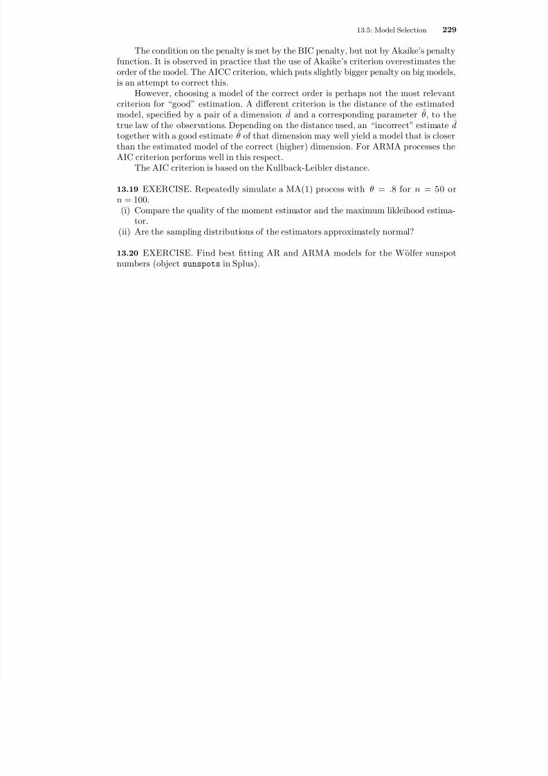
8/13/2019 van der Vaart: Time Series
http://slidepdf.com/reader/full/van-der-vaart-time-series 235/235
13.5: Model Selection 229
The condition on the penalty is met by the BIC penalty, but not by Akaike’s penaltyfunction. It is observed in practice that the use of Akaike’s criterion overestimates theorder of the model. The AICC criterion, which puts slightly bigger penalty on big models,is an attempt to correct this.
However, choosing a model of the correct order is perhaps not the most relevantcriterion for “good” estimation. A different criterion is the distance of the estimatedmodel, specied by a pair of a dimension d and a corresponding parameter θ, to thetrue law of the observations. Depending on the distance used, an “incorrect” estimate d
together with a good estimate θ of that dimension may well yield a model that is closerthan the estimated model of the correct (higher) dimension. For ARMA processes theAIC criterion performs well in this respect.
The AIC criterion is based on the Kullback-Leibler distance.
13 19 EXERCISE Repeatedly simulate a MA(1) process with θ = 8 for n = 50 or